Lagrangian Smoothing Heuristics for Max-Cut

Lagrangian Smoothing Heuristics for Max-Cut†

Hernan Alperin‡‡ Ivo Nowak∗

November 20, 2003‡

Humboldt-Universitat zu Berlin

Institut fur Mathematik

Rudower Chaussee 25,

D-12489 Berlin, Germany

†The work was supported by the German Research Foundation (DFG) under grant NO 421/2-1.‡‡[email protected] Numerische Mathematik, telefon (fax): +49-30-2093-5429 (2232)∗[email protected]

‡revised version, first draft from January 3, 2003

1

Abstract

This paper presents a smoothing heuristic for an NP-hard combinatorial problem. Starting

with a convex Lagrangian relaxation, a pathfollowing method is applied to obtain good solutions

while gradually transforming the relaxed problem into the original problem formulated with an

exact penalty function. Starting points are drawn using different sampling techniques that use

randomization and eigenvectors. The dual point that defines the convex relaxation is computed

via eigenvalue optimization using subgradient techniques.

The proposed method turns out to be competitive with the most recent ones. The idea

presented here is generic and can be generalized to all box-constrained problems where convex

Lagrangian relaxation can be applied. Furthermore, to the best of our knowledge, this is the

first time that a Lagrangian heuristic is combined with pathfollowing techniques.

Key words. semidefinite programming, quadratic programming, combinatorial optimiza-

tion, non-convex programming, approximation methods and heuristics, pathfollowing,

AMS classifications. 90C22, 90C20, 90C27, 90C26, 90C59

2

1 Introduction

Let G = (N, E) be an undirected weighted graph consisting of the set of nodes N and the set of arcs

or edges E. Let aij be the cost of edge ij, and assume G complete, otherwise set aij = 0 for every

edge ij not in E. The Maximum Cut problem consists of finding a subset of the nodes, S ⊂ N , that

maximizes the cut function

cut(S) =∑

ij∈δ(S)

aij ,

where the incidence function δ(S) = {ij ∈ E such that i ∈ S and j /∈ S}, is defined to be the set of

arcs that cross the boundary of S.

Let the vector x, with xi ∈ {−1, 1}, represent whether i ∈ S. In this way, ij ∈ δ(S), i.e. nodes i

and j are on different sides of the cut, if and only if xixj < 0. It is well known that the maximum

cut problem can be formulated as the following quadratic nonconvex problem,

(MC-Q)min xT Ax

subjectto Xx = e

where A is a symmetric matrix containing the costs aij , X = Diag(x) is the matrix with the vector

x in its diagonal and zeros elsewhere, and e ∈ IRn is the vector of ones. The reader who is not

familiar with the previous reformulation can observe that Xx = e if and only if x ∈ {−1, 1}n and

xT Ax =n

∑

i,j=1

xixj >0

aij −n

∑

i,j=1

xixj <0

aij =n

∑

i,j=1

aij − 2n

∑

i,j=1

xixj <0

aij = eT Ae − 4∑

ij∈δ(S)

aij .

The symmetric matrix A is related to the so-called Laplace matrix.

Regardless that problem (MC-Q) was proved to be NP-hard [11], some interesting heuristics to

obtain good solutions have been proposed. Following, we present the most known and recent ones.

Let Z < 0 be a positive semidefinite matrix in IR(n,n), diag(Z) be the vector representation of the

diagonal of the matrix Z, and A • B = trace(AB) =∑

ij aijbij , be the exhaustive sum of the ele-

ments of the Hadamard product. Problem (MC-Q) can be also written as

(MC-SDP)

min A • Z

subjectto diag(Z) = e

Z = xxT

Z < 0,

by noting that the constraint Z = xxT implies that diag(Z) = Xx, and that trace(AZ) =

trace(AxxT ) = xT Ax. By removing the rank-1 constraint Z = xxT , we have the semidefinite

3

relaxation problem

(SDP)

min A • Z

subjectto diag(Z) = e

Z < 0.

Goemans and Williamson [12] used the solution of (SDP) to generate random feasible points x.

Assuming that Z∗ is a (SDP) optimal solution, which is not necessarily rank-1, their strategy consists

of finding a factorization Z∗ = V T V , where V can be the Choleski factorization, for example. A

feasible solution x = sign(V T u) can be produced using the random vector u ∼ U [B(0, 1)], uniformly

distributed over the zero centered n dimensional ball of radius one. For the case of non-negative edge

weights, aij ≥ 0, they proved a bound on the expected value of the randomly generated solutions,

that is

E(xT Ax) ≥ .878 val(MC-Q),

where val(MC-Q) is the optimal value of problem (MC-Q), and E(xT Ax) is the expected value of

the objective function of (MC-Q) using the randomly generated feasible point x.

Later Bertsimas and Ye [5] proved that it is possible to use the SDP optimal solution, Z∗, as a

covariance matrix to generate a vector x ∼ N(0, Z∗). This randomly generated vector can be used

to produce a feasible one, x = sign(x), leading to the same results. A similar procedure for rounding

solutions of SDP relaxations was proposed by Zwick [26].

Unfortunately, solving problem (SDP) by means of a primal-dual interior point algorithm can require

quite a long time if the problem contains thousands of variables. Besides, the sparsity of the matrix is

lost when the problem is solved by that method. Several SDP methods exploiting sparsity have been

proposed, such as the purely dual interior point algorithm [2], nonlinear programming approach [7],

and the spectral bundle method [17].

Burer et al. [6] have devised a rank-2 relaxation of problem (MC-Q). In their heuristic, they relax

the binary vector into a vector of angles, and work with an angular representation of the cut. They

maximize an unconstrained sigmoidal function to obtain heuristic points, that later are perturbed

to improve the results of the algorithm. Their approach is similar to the Lorena [3] algorithm. Festa

et al. [10] proposed several heuristics called greedy randomized adaptive search procedure (GRASP)

and variable neighborhood search (VNS) that work very good to find near optimum solution for the

Max-Cut problem. We compare our heuristic with these methods.

The Max-Cut problem can also be formulated as an unconstrained quadratic binary problem,

4

(UQB) [16, 21]. Metaheuristics for solving UQB are proposed and studied for cases containing

up to 2500 variables [1].

In this paper, we propose a pathfollowing heuristic, which is also called deformation, or smoothing

heuristic. The heuristic is based on a parametric optimization problem defined as a convex com-

bination between a Lagrangian relaxation and the original problem. Starting from the Lagrangian

relaxation, a pathfollowing method is applied to obtain good solutions while gradually transforming

the relaxed problem into the original problem formulated with an exact penalty function.

Paths of this parametric optimization problem are traced using a projected gradient method and the

final points are rounded. To follow this idea, starting points for the procedure are needed. Hence,

we present different sampling techniques to generate the initial points.

This method aims to avoid regions with less interesting local optima, while focusing on regions where

the global optimum is likely to be. Such kinds of heuristics have been applied to energy optimization

problems, where the relaxation is obtained using Gaussian transformations. Scheltstraete et al. [24]

provide an overview on this kind of heuristic. Approaches also based on interior point methods are

suggested by Warners in his thesis [25].

Feltenmark and Kiwiel [9] proposed a Lagrangian heuristic which can be applied to very general

optimization problems. In that paper, they observed that higher dual objective accuracy need not

necessarily imply better quality of the heuristic primal solution. Our results from the sampling

spaces also pose questions regarding the importance of solving the dual problem until optimality.

We obtain good solutions with our heuristic by using feasible dual points that are not necessary

close to optimality. In many cases, eigenvalue corrected dual points already yield good results.

The paper is organized in six sections. The next section describes how convex Lagrangian relaxations

of problem (MC-Q) are generated and explains the dual formulation, which gives grounds to some

sampling techniques proposed later. Section 3 introduces the main idea of the paper by defining the

pathfollowing heuristic and describing its parameters. Section 4 explains the sampling methods for

generating starting points for the algorithm. Finally, section 5 presents the results and a comparison

to the state of the art algorithms. Our conclusions are presented in section 6.

5

2 Convex Lagrangian Relaxation

Before describing the main algorithm, we need to explain how relaxations of problem (MC-Q) can

be obtained using duality theory. We first formulate the Lagrangian dual, then transform it to its

eigenvalue formulation, and describe how it can be optimized using bundle or other subgradient

methods for nonsmooth optimization. The theoretical background for this section is well known,

and can be found for example in [4].

The Lagrangian function of problem (MC-Q) can be written as

L (x; µ) = −eT µ + xT (A + M)x,

where M = Diag(µ), µ ∈ IRn is a vector of Lagrangian multipliers. The dual function,

D(µ) = infx∈IRn

L (x; µ) ,

can be clearly written in closed form as

D(µ) =

−eT µ if A + M < 0

−∞ if A + M 6< 0.(1)

Finally, the Lagrangian dual problem of (MC-Q) is

(D) supµ∈IRn

D(µ).

The closed form (1) shows that for each µ ∈ domD the Lagrangian L(·; µ) is a convex underestimator

of the objective function over [−e, e]. Note also that (D) is equivalent to the semidefinite program

(D-SDP)max −eT µ

s.t. A + M < 0,

which is the dual of (SDP). The related duality gap is zero since the Slater condition holds. It is

interesting to note that solving problem (D-SDP) is actually the task of finding the minimum sum

of elements to set in the diagonal of A such that it becomes positive semidefinite: min∑

µi such

that A + M < 0.

The following result is well known [16].

Lemma 1 The optimum of problem (D-SDP) is attained when the smallest eigenvalue of A + M is

zero.

Let us assume that A + M � 0. This means that all its eigenvalues are positive. Let ω > 0 be the

6

smallest of the eigenvalues of A+M . We can define M ∗ = M −ωI with A+M∗ = A+M −ωI < 0.

Hence, eT µ∗ = eT µ − nω < eT µ, showing that µ could not have been the optimum. �

The dual problem (D) can also be formulated as the following eigenvalue optimization problem. We

define the dual function with respect to S = {x ∈ IRn | ‖x‖2 = n}, the smallest sphere that contains

the feasible set, {−1, 1}n ⊂ S.

DS(µ) = minx∈S

L (x; µ) = −eT µ + nλ1(A + M), (2)

where λ1(Q) denote the smallest eigenvalue of Q, and the corresponding dual problem is therefore

(DS) supµ∈IRn

DS(µ) = supµ∈IRn

minx∈S

L (x; µ) = supµ∈IRn

−eT µ + nλ1(A + M).

We can state the following relationships between solutions of (D) and (DS).

Proposition 1

(i) It holds that D(µ − λ1(A + M)e) = DS(µ).

(ii) The optimum values of (D) and (DS) are the same.

(iii) If µ is a solution of (DS) then µ∗ = µ − λ1(A + M)e is a solution of (D).

Proof.

(i) Given ω = λ1(A + M), the matrix A + M − ωI is clearly positive semidefinite. From the closed

form (1) of the dual function, it follows D(µ − ωe) = −eT (µ − ωe) = −eT µ + nω = DS(µ).

(ii) From Lemma 1, A solution µ of (D) fulfills λ1(A + M) = 0. Hence, val(D) = val(DS) follows

from (i).

(iii) follows from (i) and (ii). �

Remark 1 The transformation µ∗ = µ−λ1(A+M)e maps an arbitrary µ ∈ IRn onto dom D, which

is the convex set where A + M � 0. Thus, the Lagrangian L (x; µ∗) = −eµ∗ + xT (A + M)x is a

convex function.

2.1 Supergradient formula

The unconstrained problem (DS) can be solved using super- or subgradient optimization techniques.

A supergradient of a not-necessarily differentiable concave function D :IRm → IR, is a vector g ∈ IRm,

7

satisfying

D(µ) + gT (λ − µ) ≥ D(λ)

for all λ, µ ∈ IRm. The previous definition is widely known in its reverse form for convex functions

and subgradients. A supergradient of a dual function can be computed by evaluating the constraint

functions at a Lagrangian solution point. The following lemma holds [18]:

Lemma 2 Let L(x; µ) = f(x)+µT h(x) be a continuous Lagrangian function related to an objective

function f :IRn → IR and a constraint function h :IRn → IRm. Let X ⊂ IRn be a compact set. Then

the dual function D(µ) is concave and the vector gµ = h(xµ) ∈ IRm is a supergradient of D(µ) at

µ ∈ dom (D), where xµ is a Lagrangian solution of D(µ), i.e.

xµ ∈ Argminx∈X

L(x; µ).

The previous result can be applied as follows.

Proposition 2 For a given dual point µ ∈ IRn, let v ∈ IRn be a minimum eigenvector of A + M ,

with ‖v‖ = 1, and let xµ = n1/2v be a solution of the Lagrangian problem (2). Then gµ ∈ IRn,

defined by gµ = Xµxµ − e, is a supergradient of DS(µ) at µ.

Proof. The statement follows directly from Lemma 2. �

The sequence of supergradients Xµxµ − e is used in Section 4.5 to generate a set of initial points for

the pathfollowing algorithm.

3 Pathfollowing Heuristics

A pathfollowing method works by solving a series of parameterized problems, whose solutions con-

verge to a solution of the original problem. During this process some (or all) paths from solutions

of the first parameterized problem to solutions of the original problem are followed. Based on this

idea, we present now a heuristic for problem (MC-Q).

3.1 Parametric formulation

Let us define the following box constrained parametric problem using a quadratic penalty function,

8

(MC-Pγ)min xT Ax + γ(n − ‖x‖2)

s.t. x ∈ [−e, e],

which is equivalent to (MC-Q) for γ sufficiently large. Note that if γ ≥ λn(A), the largest eigenvalue

of A, the problem (MC-Pγ) becomes concave, and therefore it attains its optima at extreme points.

Let t ∈ [0, 1] be the pathfollowing parameter, and let us set the penalty parameter γ = (1− t)−1 to

ensure γ is large enough when t is sufficiently close to 1. Let P (x; t) = xT Ax + (1− t)−1(n−‖x‖2),

be the objective function of (MC-Pγ), with γ = (1 − t)−1, an exact penalty for x ∈ [−e, e] and t

sufficiently close to 1. Let L(x; µ) = −eT µ + xT (A + M)x be the Lagrangian function regarding the

binary constraints. We can now define a convex combination with parameter t, between the penalty

objective function of problem (MC-Pγ), P (x; t), and the Lagrangian L (x; µ), to be

H(x; µ, t) = tP (x; t) + (1 − t)L(x; µ)

= t(1 − t)−1n − (1 − t)eT µ + xT (A − t(1 − t)−1I + (1 − t)M)x. (3)

The formulation (3) shows that the function H is quadratic on x. Finally, we consider the following

parametric optimization problem associated to the pathfollowing function,

(Pt) minx∈[−e,e]

H(x; µ, t).

This formulation is used to trace paths of solutions of problem (Pt) when t → 1.

Assuming that µ ∈ dom D, the function H(·; µ, 0) = L(·; µ) is a convex underestimator of (MC-Q)

and (P0) is a convex optimization problem. On the other hand, when t → 1, H(·; ·, t) → P (·; t),

which becomes concave for t close to 1. The latter motivates the following Lemma.

Lemma 3

There exists t0 ∈ (0, 1) such that val(MC-Q) = val(Pt) for all t ∈ [t0, 1).

Proof. Let us see that there exists t0 ∈ (0, 1) such that H(·; µ, t) is concave for t ∈ [t0, 1). Consider

the Hessian ofH(x; µ, t), from the formulation (3), ∇2H = 2(A − t(1 − t)−1I + (1 − t)M). Since

t(1 − t)−1 → ∞ when t → 1, the matrix ∇2H is negative definite for some t0 < 1. Furthermore,

H(x; µ, t) = xT Ax for all x ∈ {−1, 1}n, for all µ ∈ IRn, and t ∈ IR, which proves the statement. �

Remark 2 Note that it might be possible that the path x(t) of the parametric optimization problem

(Pt) related to a solution x∗ of (MC-Q) is discontinuous [15].

9

Remark 3 Dentcheva et al. [8] and Guddat et al. [14] pointed out general disadvantages of these

formulations, i.e. the one-parameter optimization is not defined for t = 1, and the objective func-

tion could be only once continuously differentiable. However, for the Max-Cut problem the penalty

objective function used is quadratic, thus infinitely many times differentiable since no inequality con-

straints were used. On the other side, from Lemma 3, the path need not to be traced until t = 1,

disregarding that undefined point.

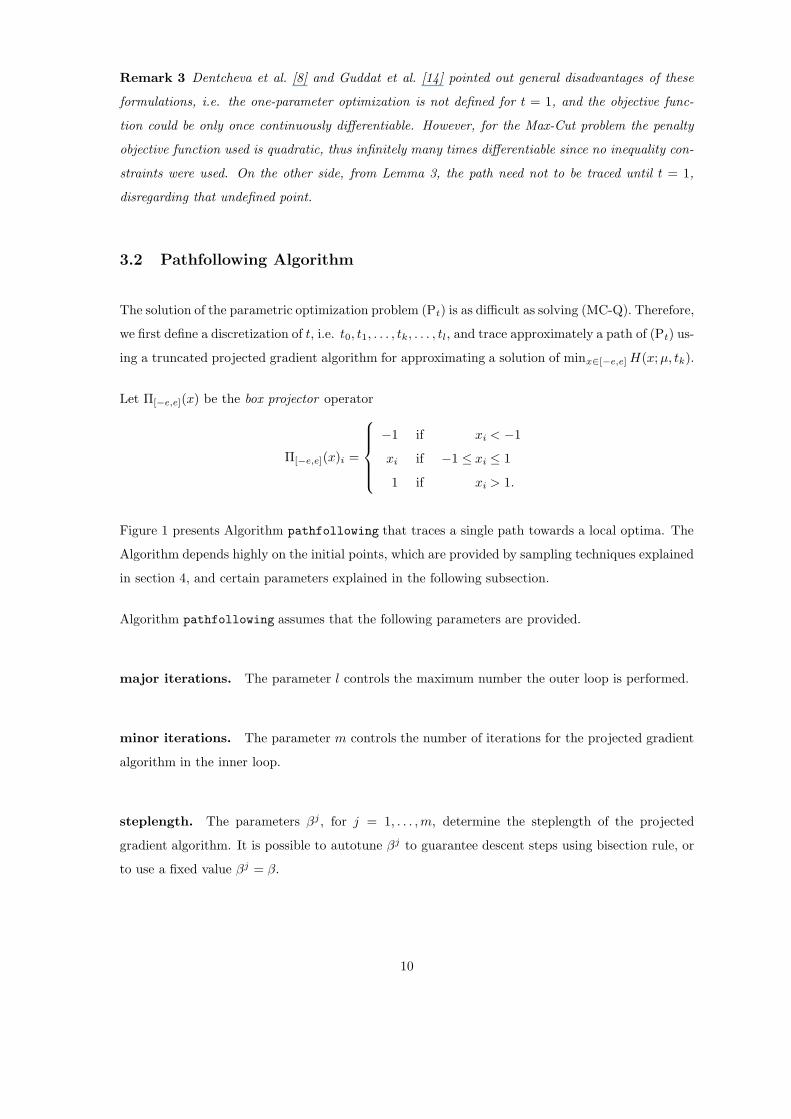
3.2 Pathfollowing Algorithm

The solution of the parametric optimization problem (Pt) is as difficult as solving (MC-Q). Therefore,

we first define a discretization of t, i.e. t0, t1, . . . , tk, . . . , tl, and trace approximately a path of (Pt) us-

ing a truncated projected gradient algorithm for approximating a solution of minx∈[−e,e] H(x; µ, tk).

Let Π[−e,e](x) be the box projector operator

Π[−e,e](x)i =

−1 if xi < −1

xi if −1 ≤ xi ≤ 1

1 if xi > 1.

Figure 1 presents Algorithm pathfollowing that traces a single path towards a local optima. The

Algorithm depends highly on the initial points, which are provided by sampling techniques explained

in section 4, and certain parameters explained in the following subsection.

Algorithm pathfollowing assumes that the following parameters are provided.

major iterations. The parameter l controls the maximum number the outer loop is performed.

minor iterations. The parameter m controls the number of iterations for the projected gradient

algorithm in the inner loop.

steplength. The parameters βj , for j = 1, . . . , m, determine the steplength of the projected

gradient algorithm. It is possible to autotune βj to guarantee descent steps using bisection rule, or

to use a fixed value βj = β.

10

Algorithm x = pathfollowing(x, µ)

set k := 0;

t0 := 0;

x0 := x;

do get tk+1 > tk;

set y0 := xk;

for j := 0 to m − 1 do

yj+1 := Π[−e,e]

„

yj − βj ∇H(yj ; µ, tk)

‖∇H(yj ; µ, tk)‖

«

;

set k := k + 1;

xk = ym;

until stopping criteria fulfilled or k = l;

return x = sign(xk).

Figure 1: Algorithm pathfollowing traces a path from a starting primal point x to a feasible

point x. The parameters l, m, βj , tk are explained in more detail below. The inner loop solves

approximately xk = argminx∈[−e,e] H(x; µ, tk) by making m steps (minor iterations) of a projected

gradient algorithm.

discretization sequence. The parameters t1 < · · · < tk < · · · < tl, determine the values at which

the function H(x; µ, tk) is optimized. It is possible to generate tk, using a geometric sequence, i.e.

tk = 1− ρk with ρ ∈ (0, 1), or using a uniform sequence, i.e. tk = k/(l + 1).

The following proposition based on Lemma 3 provides grounds for the stopping criteria. It is

important to note that the algorithm proposed stops when it finds a local optimum of the Max-Cut

problem. Despise the fact that global optimality can not be guaranteed, we expect the proposed

heuristic provides good local solutions.

Proposition 3 If m is large enough, Algorithm pathfollowing can be stopped if tk ≥ t0 without

changing the final result, where t0 is defined in the proof of Lemma 3.

Proof. If tk ≥ t0 from Lemma 3, then H(·; µ, tk) is concave. Clearly, in this case, the projected

gradient algorithm successively makes binary constraints active and therefore converges in finitely

many steps to a vertex. �

Let x∗ be the global optimum of problem (MC-Q). We define the region of attraction to be the set

of points x such that sign(x) = sign(x∗). With the previous proposition, it is not needed to follow

the path until the end, since after tk > t0 with m large enough, xk is in a region of attraction and

its projection will not change for larger k.

11

4 Sampling

Algorithm pathfollowing requires initial dual and primal points. Since the algorithm is a heuristic,

better results are not necessarily achieved by better dual points and their corresponding Lagrangian

solutions. Therefore, we devised several techniques for generating sample points in the primal and

dual space. The following subsections describe how a single dual vector µ and its corresponding

primal point x are generated in each sampling method. We define two kinds of sampling methods,

the first over the primal space using random techniques on different spaces, and the second over

the dual space, using a sequence from an optimization algorithm. The sampling is repeated up to

complete the defined sample size.

A sample of size p to start Algorithm pathfollowing can be represented as a set of pairs of primal

and dual points, S = {(xi, µi) with i = 1, . . . , p}. The primal sampling sets are those whose dual

points, µi = µ, are the same through the sample. Respectively, the dual sampling sets are those

whose dual points vary through the sample or some dual method was used to obtain them. We start

describing first sampling on the primal space, and we follow with the sampling in the dual space.

4.1 Random primal

A starting primal point is chosen with uniform random distribution over the ball B(0, n1/2). Then,

Algorithm pathfollowing is applied with µ = −λ1(A)e. This is the simplest of all the sampling,

since it does not compute the primal from dual information.

The random primal sample is therefore,

SRP = {(xi, µ) : i = 1, . . . , p, xi ∼ U [B(0, n1/2)], µ = −λ1(A)e},

where xi ∼ U [S], means that the sample point xi is independently drawn with uniform random

distribution over the set S.

4.2 Preswitching

This is also a primal sampling, since no dual sequence is used, i.e. we do not attempt to solve the

dual when generating this sample. We use the eigenvector corresponding to the smallest eigenvalue

of A, v1(A) = v1(A + M), where M = −λ1(A)I .

We define a threshold ε for all components of the primal point. If |xi| < ε, we multiply its value by

12

-1 with a probability one half. This is done to explore the opposite direction when a component of

the primal starting point is close to zero.

The preswitching sample is then,

SP = {(xi, µ) : i = 1, . . . , p, xi = ρχε(v1(A)), µ = −λ1(A)e},

where ρ = n1/2/‖v1(A)‖, and χε(v) is a random vector defined as

χε(x)j =

xj if |xj | ≥ ε

ujxj if |xj | < ε,

and uj are independent identically distributed Bernoulli random variables, which take values in

{−1, 1} with probability one half each.

4.3 Eigenspace sampling

If the duality gap, i.e. the difference between the optimum value of problems (MC-Q) and (D), is

zero, then an optimum primal solution lies in the eigenspace of the minimum eigenvalue. Motivated

by this fact, we generate random points in the space spanned by the eigenvectors that correspond

to a certain number of smallest eigenvalues. This is particularly helpful to increase the space of

the sample if the difference in value between them is small, or if the smallest eigenvalue has large

multiplicity.

In particular, we define

SE = {(xi, µ) : i = 1, . . . , p, xi = n1/2yi/‖yi‖, µ = −λ1(A)e},

where

yi =r

∑

k=1

αkvk(A + M),

and αk ∼ N(0, 1), independent normally distributed, and vi(·) is the eigenvector corresponding to

the i-th lowest eigenvalue. The resulting random linear combination of eigenvectors, yi is projected

onto B(0, n1/2), the ball that contains the [−e, e] box.

This sampling can be combined to any sampling on the dual space by having different dual points

µi for i = 1, . . . , p, or just by selecting a single different dual point. We explain this in section 4.6 on

page 15.

13

4.4 Random duals

This and the following, are sampling using different dual points.

To check the importance of solving the dual problem to generate good heuristic primal solutions,

we generated independent random points normally distributed in the dual space, ν i ∼ N(0, σI),

independent identically distributed. Then, we constructed the sample correcting the dual points as

explained in Remark 1,

SRD = {(xi, µi) : i = 1, . . . , p, xi = ρiv1(A + M i), µi = νi − λ1(A + N i)e},

where ρi = n1/2/‖v1(A + M i)‖, and N = Diag(ν). We map the dual points onto the semidefinite

cone by subtracting the lowest eigenvalue times the vector of ones, µi = νi −λ1(A+N i)e, to ensure

the convexity of the Lagrangian.

Another possible way to guarantee the convexity of L(x; µ), is to use Gershgorin sufficient condition

of positive semidefiniteness, A + M < 0 is implied by

µi ≥∑

i6=j

|aij |

since aii is zero in the Max-Cut case. However, we believe eigenvalue convexification is better. On

the other side, the latter method is faster.

4.5 Dual sequence

A nonsmooth optimization method is applied on the unconstrained dual problem (DS). This can

range from simple supergradient methods, using steepest descent or conjugate supergradients, to

proximal bundle method. Supergradients are computed as described in Proposition 2. Let {νj}, for

j = 0, 1, . . . , be a sequence that converges towards the optimum dual value µ∗. The dual sequence

sample can be described as

SSD = {(xi, µi) : i = 1, . . . , p, xi = ρiv1(A + M i), µi ∈ {νj}j=0,1,...},

where ρi = n1/2/‖v1(A + M i)‖. Each sample dual µi is an iterate of the dual optimization method

towards obtaining the optimum dual µ∗. We pick a sample point every K iterations of the dual, i.e.

µi = νiK .

14

4.6 Eigenspace after dual termination

In this last sampling, we produce starting primal points in the eigenspace of the same dual point.

Here we generate the dual point by optimizing the dual problem until a convergence criterion is

fulfilled, ‖µk − µ∗‖ < ε, using bundle method [20].

The sample can be defined as

SED = {(xi, µ) : i = 1, . . . , p, xi = ρiyi, µ = µ∗ − λ1(A + M∗)e},

where ρi = n1/2/‖yi‖, yi =∑r

k=1 αkvk(A + M∗), and µ∗ an optimum dual, or in fact, sufficiently

close to it. The primal points are sampled from the space generated by the eigenvectors corresponding

to the smallest eigenvectors of A + M ∗, explained in section 4.3 on page 13.

5 Numerical Results

Algorithm pathfollowing was coded in C++ and compiled with g++, the GNU compiler. Super-

gradients for the dual function explained in section 2 were computed according to Lemma 2. For

the computation of the minimum eigenvalue and corresponding eigenvector we used the Lanczos

method ARPACK++ [13]. For solving the dual problem, we used Kiwiel’s proximal bundle algorithm

NOA 3.0 [19, 20]. Pseudorandom numbers were generated using RANLIB library routines to simulate

the proposed distributions.

The algorithm was tested using a set of examples from the 7th DIMACS Implementation Chal-

lenge [23], and using several instances created with rudy, a machine independent graph generator

written by G. Rinaldi, which is standard for maximum cut problem [17].

The tests were run on a machine that has two 700MHz Pentium III processors and 1Gb RAM. The

sampling size for all the sample sets was set to 10, and the best result over each sample type was

reported.

Table 1 and Table 2 show the results for the different sampling techniques. The first reports the

computing time and the second, the value in percentage refereed to the most elaborated sample

SED, eigenspace after dual termination, for which the absolute result is reported. For the reported

runs, we used a fixed number of major iterations l, a fixed steplength β, and a uniform sequence tk,

explained in section 3.2 on page 10.

Other combinations of the parameters described in section 3.2 on page 10 were tried. In particular, we

15

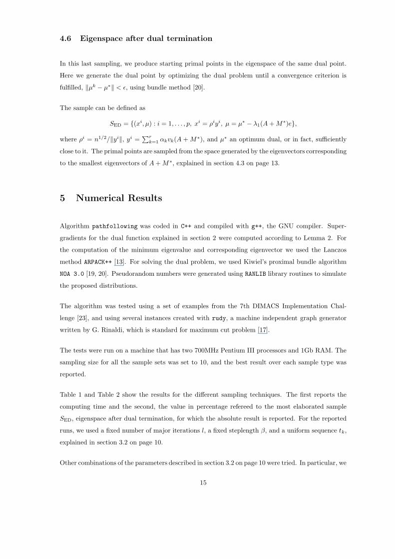
example size primal sampling dual sampling

name n m SRP SP SE SRD SSD SED

g3 800 19176 15 15 17 19 1:20 32

g6 800 19176 14 14 16 16 49 1:13

g13 800 1600 4 5 6 7 17 12:46

g14 800 4694 5 5 6 6 20 2:30

g19 800 4661 5 5 6 6 15 1:11

g23 2000 19990 24 24 29 32 1:59 2:50

g31 2000 19990 22 22 28 25 1:45 11:40

g33 2000 4000 15 15 20 30 2:47 3:27:25(†)

g38 2000 11779 17 18 21 19 1:28 9:02

g39 2000 11778 18 17 20 19 1:56 5:13

g44 1000 9990 10 10 13 17 46 1:04

g50 3000 6000 25 24 36 1:05 1:32 55

g52 1000 5916 7 7 8 8 42 3:14

Table 1: Comparison of computing time. Primal samples: SRP random primal, SP preswitching,

SE eigenspace; dual samples: SRD random dual, SSD dual sequence, and SED eigenspace after dual

stop. The columns report the computing time in hh:mm:ss, hh hours, mm minutes, and ss seconds.

mm reported when total seconds were more than 60, and similarly with hh. The run was performed

with fixed steplength β = 5, minor iterations n = 10, major iteration horizon M = 20, uniform

update on t, i.e. t values: 1/(M + 1), . . . , M/(M + 1). (†) The excessive running time was due to

the stopping criterion explained in section 3.2 on page 11.

experimented with modifications of the steplength update rule to perform line search, the sequence

of values for t (a geometric sequence for tk = 1 − ρk was also tested), and the outer loop stopping

rule explained in section 3.2 on page 11. However, we did not observed significant differences in the

results. One exception was the use of the simplest stopping rule criterion. In that particular case,

for few primal sample examples, the algorithm stopped before achieving as good results as reported.

Previous evidence with other Lagrangian heuristics for the unit commitment problem suggests that

higher dual objective accuracy need not necessarily imply better quality of the heuristic primal

solution [9]. To evaluate the importance of the information provided by the dual for the heuristic,

we plot comparatively the dual sequence and its corresponding heuristic primal solution sequence

for some graph examples in Figure 2.

We observe that meanwhile the dual improves its value, reducing the duality gap, the heuristic

16

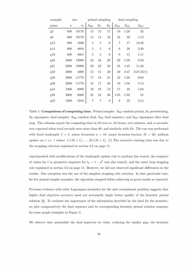
example primal sampling dual sampling dual G-W

name SRP SP SE SRD SSD SED bound E(cut)

g3 99 99 99 99 99 11608 12084 10610

g6 99 100 100 100 100 2135 2656

g13 100 100 100 100 99 568 647

g14 99 99 99 99 99 3024 3192 2803

g19 98 98 98 99 102 868 1082

g23 99 99 99 100 99 13234 14146

g31 100 100 100 100 100 3170 4117

g33 99 99 100 99 98 1342 1544

g38 99 99 99 99 99 7512 8015 7037

g39 98 99 98 99 100 2258 2877

g44 99 99 99 100 100 6601 7028 6170

g50 98 100 99 99 100 5830 5988 5257

g52 100 99 100 100 100 3779 4009 3520

Table 2: Comparison of solution quality. The first column shows the name of the problem.

The following five columns are divided in primal samples (SRP random primal, SP preswitching,

SE eigenspace) and dual samples (SRD random dual, SSD dual sequence, and SED eigenspace after

dual stop). The first five columns show the best case in percentage of the best value from the last

sampling technique SED, in the last column whose result is reported in absolute value. The last

two columns provide information about the dual bound and the expected cut using Goemans and

Williamson heuristic. The expected cut was computed only for those graphs with non-negative edge

weights. The run was performed with the same parameters as the previous table.

primal sequence is not monotonically decreasing, meaning that dual points closer to the optimum

do not necessarily provide better heuristic primal points.

Table 3 shows a comparison with rank-2 and GRASP algorithm [10] The numbers from rank 2 were

extracted from the paper [6] from the table without the use of the random perturbation. There the

results were obtained from a sample of size 1. In that paper, they report better results. However,

we were not able to reproduce those results, since we did not know the information regarding the

random perturbation parameters.

17

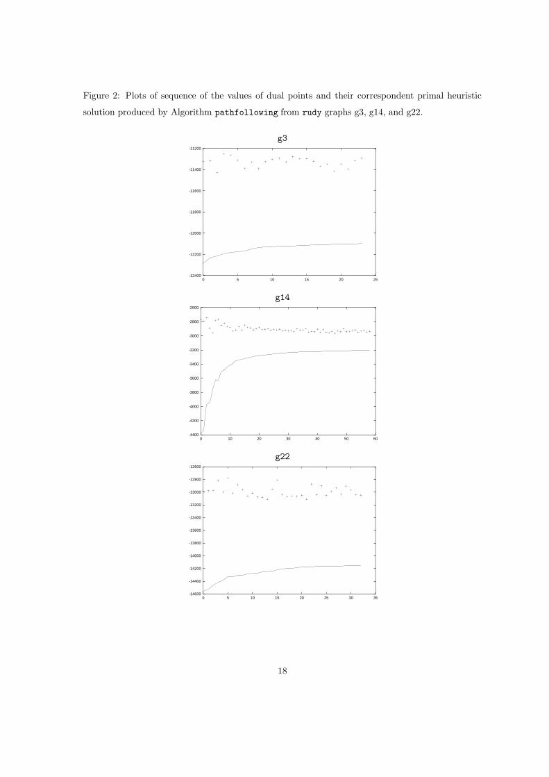
Figure 2: Plots of sequence of the values of dual points and their correspondent primal heuristic

solution produced by Algorithm pathfollowing from rudy graphs g3, g14, and g22.

g3

-12400

-12200

-12000

-11800

-11600

-11400

-11200

0 5 10 15 20 25

g14

-4400

-4200

-4000

-3800

-3600

-3400

-3200

-3000

-2800

-2600

0 10 20 30 40 50 60

g22

-14600

-14400

-14200

-14000

-13800

-13600

-13400

-13200

-13000

-12800

-12600

0 5 10 15 20 25 30 35

18

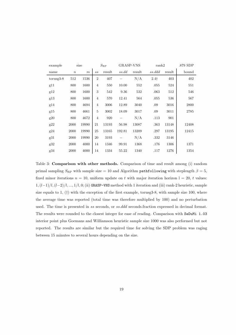
example size SRP GRASP-VNS rank2 .879 SDP

name n m ss result ss.dd result ss.ddd result bound

torusg3-8 512 1536 2 407 − N/A 2.4† 403 402

g11 800 1600 4 550 10.00 552 .055 524 551

g12 800 1600 3 542 9.36 532 .063 512 546

g13 800 1600 4 570 12.41 564 .055 536 567

g14 800 4694 4 3006 12.89 3040 .09 3016 2800

g15 800 4661 5 3002 18.09 3017 .09 3011 2785

g20 800 4672 4 920 − N/A .113 901

g22 2000 19990 21 13193 56.98 13087 .363 13148 12408

g24 2000 19990 25 13165 192.81 13209 .297 13195 12415

g31 2000 19990 20 3193 − N/A .332 3146

g32 2000 4000 14 1346 99.91 1368 .176 1306 1371

g34 2000 4000 14 1334 55.22 1340 .117 1276 1354

Table 3: Comparison with other methods. Comparison of time and result among (i) random

primal sampling SRP with sample size = 10 and Algorithm pathfollowing with steplength β = 5,

fixed minor iterations n = 10, uniform update on t with major iteration horizon l = 20, t values:

1, (l−1)/l, (l−2)/l, ..., 1/l, 0; (ii) GRASP-VNSmethod with 1 iteration and (iii) rank-2 heuristic, sample

size equals to 1, (†) with the exception of the first example, torusg3-8, with sample size 100, where

the average time was reported (total time was therefore multiplied by 100) and no perturbation

used. The time is presented in ss seconds, or ss.ddd seconds.fraction expressed in decimal format.

The results were rounded to the closest integer for ease of reading. Comparison with SeDuMi 1.03

interior point plus Goemans and Williamson heuristic sample size 1000 was also performed but not

reported. The results are similar but the required time for solving the SDP problem was raging

between 15 minutes to several hours depending on the size.

19

6 Conclusion

We presented a new heuristic for Max Cut, combining Lagrangian relaxation techniques with pathfol-

lowing methods. The results we obtained are compared with previous results obtained by Semidef-

inite Programming using interior point algorithms, like SeDuMi, and special case algorithms like

rank-2. Apparently, the new method performs competitively with techniques previously mentioned.

The experienced running time is in the examples tested better than the one from interior point

algorithm. However, it is not as good as the one from special purpose algorithm such as rank-2 from

Burer et al. [6], but it has similar performance as GRASP-VNS from Festa et al. [10].

To the best of our knowledge, it is the first time that a Lagrangian heuristic is combined with

smoothing techniques. Since the approach is generic it can be generalized to all box-constrained

problems for which a convex (Lagrangian) relaxation is available. Note that it is always possible to

shift the constraints into the objective using a penalty term. Examples for QQP and MINLP can

be found in [22], and in [21] where the second author shows that convex Lagrangian relaxations of

general mixed integer quadratic programs can be obtained by solving an eigenvalue optimization

problem. In order to apply Algorithm pathfollowing to this case the inner minimization and

rounding has to be replaced by appropriate descent methods. This is currently under investigation.

Furthermore, there are several possibilities to accelerate the proposed method. First, decomposition

techniques can be applied to solve the dual [21]. Second, Algorithm pathfollowing could be modi-

fied to trace the paths of all sample points simultaneously and delete candidates with high function

values in an early stage of the pathfollowing. This approach is also well suited for parallelization.

It would be interesting to find out for which optimization problems the dual helps the algorithm to

find better heuristic solutions. Similarly as discussed by Burer et al. [6], we found out that in the

case of Max-Cut it might not be needed to solve the dual problem to improve the quality of heuristic

solutions. It seems that the structure of the convex underestimators are not changed significantly by

solving the dual. However, Max-Cut can be considered as a highly symmetric concave optimization

problem with simple box-constraints. The situation could change for other optimization problems

with more complicated constraints.

Acknowledgment. We would like to thank Prof. Kiwiel for making NOA 3.0 available, and

Stefan Vigerske, who helped us with the C++ coding and Linux scripting. We also like to thank two

anonymous referees for their critics to our first draft.

20

References

[1] J. E. Beasley, Heuristic Algorithms for the Unconstrained Binary Quadratic Programming

Problem, tech. rep., The Management School, Imperial College, London SW7 2AZ, England,

1998.

http://mscmga.ms.ic.ac.uk/jeb/jeb.html.

[2] S. J. Benson, Y. Ye, and X. Zhang, Solving large-scale sparse semidefinite programs for

combinatorial optimization, SIAM J. Optim., 10(2) (2000), pp. 443–461.

[3] A. Berloni, P. Campadelli, and G. Grossi, An approximation algorithm for the maxi-

mum cut problem and its experimental analysis, Proceedings of “Algorithms and Experiments”,

(1998), pp. 137–143.

[4] D. P. Bertsekas, Non-linear programming, Athena Scientific, Belmont, MA, 1995.

[5] D. Bertsimas and Y. Ye, Semidefinite relaxations, multivariate normal distributions, and

order statistics, in Handbook of Combinatorial Optimization, D.-Z. Du and P. Pardalos, eds.,

Kluwer Academic Publishers, 1998, pp. 1–19.

[6] S. Burer, R. D. C. Monteiro, and Y. Zhang, Rank-two relaxation heuristics for max-cut

and other binary quadratic programs, SIAM J.Opt., 12 (2001), pp. 503–521.

[7] S. Burer and R. M. Monteiro, A nonlinear programming algorithm for solving semidefinite

programs via low-rank factorization, Mathematical Programming (Series B), 95 (2003), pp. 329–

357.

[8] D. Dentcheva, J. Guddat, and J.-J. Ruckmann, Pathfollowing methods in nonlinear

optimization III: multiplier embedding, ZOR - Math. Methods of OR, 41 (1995), pp. 127–152.

[9] S. Feltenmark and K. C. Kiwiel, Dual applications of proximal bundle methods including

lagrangian relaxation of nonconvex problems, SIAM J. Optim., 10(3) (2000), pp. 697–721.

[10] P. Festa, P. M. Pardalos, M. G. C. Resende, and C. C. Ribeiro, Randomized heuristics

for the max-cut problem, Optimization Methods and Software, 7 (2002), pp. 1033–1058.

[11] M. R. Garey and D. S. Johnson, Computers and Intractability: A Guide to the Theory of

NP-Completeness, W.H. Freeman, New York, 1979.

[12] M. X. Goemans and D. P. Williamson, Improved Approximation Algorithms for Maximum

Cut and Satisfiability Problems Using Semidefinite Programming, J. ACM, 42 (1995), pp. 1115–

1145.

21

[13] F. Gomes and D. Sorensen, ARPACK++: a C++ Implementation of ARPACK eigenvalue package,

1997.

http://www.crpc.rice.edu/software/ARPACK/.

[14] J. Guddat, F. Guerra, and D. Nowack, On the role of the Mangasarian-Fromovitz con-

straints qualification for penalty-, exact penalty- and Lagrange multiplier methods, in Mathe-

matical Programming with Data Perturbations, A. V. Fiacco, ed., Marcel Deckker, Inc., New

York, 1998, pp. 159–183.

[15] J. Guddat, F. G. Vazquez, and H. T. Jongen, Parametric Optimization: Singularities,

Pathfollowing and Jumps, John Wiley and Sons, 1990.

[16] C. Helmberg, Semidefinite Programming for Combinatorial Optimization, tech. rep., ZIB–

Report 00–34, 2000.

[17] C. Helmberg and F. Rendl, A spectral bundle method for semidefinite programming, SIAM

J. Opt., 10(3) (2000), pp. 673–695.

[18] J. B. Hiriart-Urruty and C. Lemarechal, Convex Analysis and Minimization Algorithms

I and II, Springer, Berlin, 1993.

[19] K. C. Kiwiel, Proximity control in bundle methods for convex nondifferentiable minimization,

Math. Progr., 46 (1990), pp. 105–122.

[20] , User’s Guide for NOA 2.0/3.0: A FORTRAN Package for Convex Nondifferentiable Opti-

mization, Polish Academy of Science, System Research Institute, Warsaw, 1993/1994.

[21] I. Nowak, Lagrangian Decomposition of Mixed-Integer All-Quadratic Programs, tech. rep.,

HU–Berlin NR–2002–7, 2002.

[22] I. Nowak, H. Alperin, and S. Vigerske, LaGO - an object oriented library for solving

MINLPs, in Global Optimization and Constraint Satisfaction, C. Bliek et al., ed., Springer,

Berlin, 2003, pp. 32–42.

http://www.mathematik.hu-berlin.de/$\sim$eopt/papers/LaGO.pdf.

[23] G. Pataki and S. H. Schmieta, The DIMACS Library of Mixed Semidefinite Quadratic

Linear Programs.

http://dimacs.rutgers.edu/Challenges/Seventh/Instances/.

[24] S. Schelstraete, W. Schepens, and H. Verschelde, Energy minimization by smoothing

techniques: a survey, in From Classical to Quantum Methods, E. P. Balbuena and J. Seminario,

eds., Elsevier, 1998, pp. 129–185.

22

[25] J. P. Warners, Nonlinear Approaches to Satisfiability Problems, PhD thesis, Eidhoven Uni-

versity of Technology, 1999. Chapter 6: A Nonlinear Approach to Combinatorial Optimization.

[26] U. Zwick, Outward rotations: a tool for rounding solutions of semidefinite programming re-

laxations, with applications to max cut and other problems, in Proc. of 31th STOC, 1999,

pp. 679–687.

23