LABOUR AND GOODS MARKET DYNAMICS USING AN ABSTRACT MICROECONOMICAL MODEL

Vol. 5 (2012) Acta Physica Polonica B Proceedings Supplement No 1

LABOUR AND GOODS MARKET DYNAMICSUSING AN ABSTRACT MICROECONOMICAL MODEL∗

Ranaivo M. Razakanirina†, Bastien Chopard

Computer Science Department, University of Geneva7 route de Drize, 1227 Carouge, Switzerland

(Received December 20, 2011)

This paper presents a multilayer cellular automata on a graph to modelthe exchanges of working hours against salary coupled with the exchangesof cash against goods, thus creating an artificial labour and goods markets.During the time evolution, the cooperation and the competition betweenthe individuals create rich behaviours: the strongly connected components(SCC) of the whole market emerge, a steady state or chaotic state appears,poor and rich cells emerge. When reaching the steady state, we show alsothat the distribution of cash is, in average, proportional to the in-degree ofthe cells.

DOI:10.5506/APhysPolBSupp.5.131PACS numbers: 05.45.–a, 89.65.Gh

1. Introduction

The approach we consider to model the dynamic of an artificial mar-ket is based on the microscopic behaviours of each agent of the marketand the dynamic of the interactions between them. We model such systemusing the Multilayer Cellular Automata on a Graph formalism (MCAG for-malism) [1], a formalism which merges recent advances on the topologicalanalysis of complex network [2, 3, 4, 5, 6] and on the cellular automata onirregular topology [7, 8].

The main interest of MCAG is its ability to model systems consistingof the superposition of cellular automata on graph layers, each layer havingdistinct irregular neighbourhood topology built upon a graph. We proposein this paper a model of agents who exchange working hours against salaryand cash against goods. The model, denoted Labour–Goods Market (LGM)consists of an artificial labour market coupled with an artificial goods market.The neighbourhood topologies of both markets are distinct.∗ Presented at the Summer Solstice 2011 International Conference on Discrete Modelsof Complex Systems, Turku, Finland, June 6–10, 2011.† Corresponding e-mail address: [email protected]

(131)

132 R.M. Razakanirina, B. Chopard

This paper is organized as follows: we first describe the LGM modelthen, we present the parameters used during the simulations and finally, wediscuss the obtained results.

2. Labour–Goods Market model formalism (LGM model)

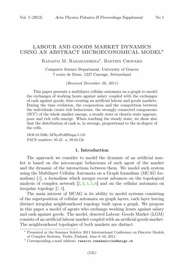
Let us denote by V the set of agents that may represent individuals.The structures of the labour and goods markets are built upon a directedgraphs denoted respectively by G`(V,E`) and Gg(V,Eg). E` and Eg are,respectively, the sets of directed edges of G` (black edges in Fig. 1) and Gg(light grey edges in Fig. 1).

Fig. 1. An example of LGM model with five agents labelled 0 to 4. V={0, 1, 2, 3, 4}.The set of black edges E` models the structure of labour market and the set of lightgrey edges Eg models the structure of goods market.

Graphs G` and Gg define the roles of each individual and its neighbour-hood. The directed edge (i, j) ∈ E` means that i is the employer of j. Thedirected edge (k, `) ∈ Eg means that k buys goods from `. Let us considercell 2 of Fig. 1 as an example. Cell 2 is the employer of 4 for the labourmarket. Cell 2 buys goods from 3 and sells goods to 4 for the goods market.

We assume that individuals are not a self-employed workers and do notbuy or sell goods to themselves. Therefore, G` and Gg are a simple di-rected graphs [9]. We denote respectively by aij and bij the elements of theadjacency matrices [4] of G` and Gg.

At each time iteration t, the state of each individual i consists of theindividual’s wealths which are (1) its available working hours hi(t), (2) itscash ci(t) and (3) the quantity of goods gi(t) it owns. These quantities areinfinitely divisible. The working hours cannot be saved and are reset to valueδi at each time iteration. For instance, if the time step is one day, δi = 8hours of work. For the labour market, the cash is used to pay the salaries ofworkers. For the goods market, the cash is used to buy goods from sellers.

Labour and Goods Market Dynamics Using an Abstract Microeconomical . . . 133

During the evolution, the agents do not create or delete cash. Thus thetotal cash ctot =

∑∀` c`(t), ∀t is conserved. However, agents produce and

consume goods.The transition function of LGM model is split naturally into two main

phases which are the labour market dynamics and the goods market dynam-ics. This transition function is applied locally and synchronously on all theagents. These phases are stated as follows:

(a) (b)

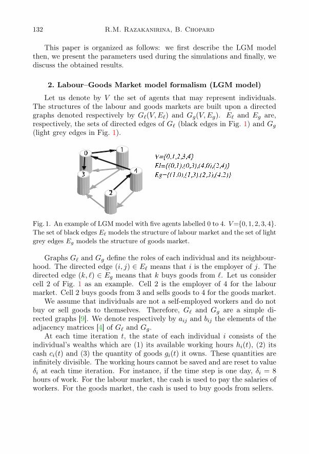
(c) (d)Fig. 2. Flows of hours (dark grey dashed edges in (a)), cash (dark grey dashededges in (b) and light grey dashed edges in (c)) and goods (light grey dashed edgesin (d)) during the transition rule of the LGM-model depicted in Fig. 1.

2.1. Labour market dynamics

During this phase, each individual spends time to work for its employers.In exchange cash is returned by the employers. The working hours spentby the individual are transformed to goods for the benefit of the employers.Let us consider a link (i, j) in the labour market. hji is the flow of hours(dark grey dashed edges of Fig. 2 (a)), cij is the flow of cash (dark greydashed edges of Fig. 2 (b)) and wij is the hourly wage offered by i to j. Thisdynamics is split as follows:


2.1.1. Exchanges of hours

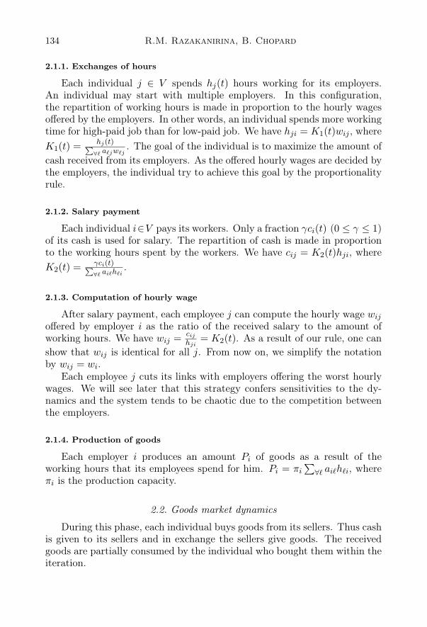
Each individual j ∈ V spends hj(t) hours working for its employers.An individual may start with multiple employers. In this configuration,the repartition of working hours is made in proportion to the hourly wagesoffered by the employers. In other words, an individual spends more workingtime for high-paid job than for low-paid job. We have hji = K1(t)wij , whereK1(t) = hj(t)P

∀` a`jw`j. The goal of the individual is to maximize the amount of

cash received from its employers. As the offered hourly wages are decided bythe employers, the individual try to achieve this goal by the proportionalityrule.

2.1.2. Salary payment

Each individual i∈V pays its workers. Only a fraction γci(t) (0 ≤ γ ≤ 1)of its cash is used for salary. The repartition of cash is made in proportionto the working hours spent by the workers. We have cij = K2(t)hji, whereK2(t) = γci(t)P

∀` ai`hì.

2.1.3. Computation of hourly wage

After salary payment, each employee j can compute the hourly wage wijoffered by employer i as the ratio of the received salary to the amount ofworking hours. We have wij = cij

hji= K2(t). As a result of our rule, one can

show that wij is identical for all j. From now on, we simplify the notationby wij = wi.

Each employee j cuts its links with employers offering the worst hourlywages. We will see later that this strategy confers sensitivities to the dy-namics and the system tends to be chaotic due to the competition betweenthe employers.

2.1.4. Production of goods

Each employer i produces an amount Pi of goods as a result of theworking hours that its employees spend for him. Pi = πi

∑∀` ai`hì, where

πi is the production capacity.

2.2. Goods market dynamics

During this phase, each individual buys goods from its sellers. Thus cashis given to its sellers and in exchange the sellers give goods. The receivedgoods are partially consumed by the individual who bought them within theiteration.


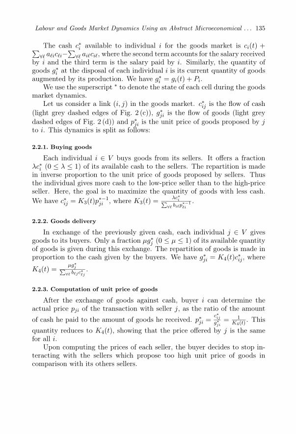
The cash c∗i available to individual i for the goods market is ci(t) +∑∀` aìcì−

∑∀` ai`ci`, where the second term accounts for the salary received

by i and the third term is the salary paid by i. Similarly, the quantity ofgoods g∗i at the disposal of each individual i is its current quantity of goodsaugmented by its production. We have g∗i = gi(t) + Pi.

We use the superscript ∗ to denote the state of each cell during the goodsmarket dynamics.

Let us consider a link (i, j) in the goods market. c∗ij is the flow of cash(light grey dashed edges of Fig. 2 (c)), g∗ji is the flow of goods (light greydashed edges of Fig. 2 (d)) and p∗ji is the unit price of goods proposed by jto i. This dynamics is split as follows:

2.2.1. Buying goods

Each individual i ∈ V buys goods from its sellers. It offers a fractionλc∗i (0 ≤ λ ≤ 1) of its available cash to the sellers. The repartition is madein inverse proportion to the unit price of goods proposed by sellers. Thusthe individual gives more cash to the low-price seller than to the high-priceseller. Here, the goal is to maximize the quantity of goods with less cash.We have c∗ij = K3(t)p∗−1

ji , where K3(t) = λc∗iP∀` bi`p

∗−1ì

.

2.2.2. Goods delivery

In exchange of the previously given cash, each individual j ∈ V givesgoods to its buyers. Only a fraction µg∗j (0 ≤ µ ≤ 1) of its available quantityof goods is given during this exchange. The repartition of goods is made inproportion to the cash given by the buyers. We have g∗ji = K4(t)c∗ij , where

K4(t) =µg∗jP∀` b`jc

∗`j.

2.2.3. Computation of unit price of goods

After the exchange of goods against cash, buyer i can determine theactual price pji of the transaction with seller j, as the ratio of the amountof cash he paid to the amount of goods he received. p∗ji =

c∗ijg∗ji

= 1K4(t) . This

quantity reduces to K4(t), showing that the price offered by j is the samefor all i.

Upon computing the prices of each seller, the buyer decides to stop in-teracting with the sellers which propose too high unit price of goods incomparison with its others sellers.


2.2.4. Consumption of goods

Each individual i ∈ V consumes with a rate φi its balance of goods. Thisbalance is the difference between the sum of goods received from its sellers∑∀` bi`g

∗ì and the sum of quantity of goods given to its buyers

∑∀` bìg

∗i`

added to the current quantity of goods at its disposal. Thus, the quantityof goods Ci consumed by individual i within the iteration is Ci = φi(g∗i +∑∀` bi`g

∗ì −

∑∀` bìg

∗i`).

2.3. State of each agent at the next time iteration

At the next time iteration, each individual i resets its available quantityof hours. Therefore

hi(t+ 1) = δi . (1)

The balance of cash of the individual i at the next time iteration t+ 1 is

ci(t+ 1) = ci(t)−∑∀ài`ci` +

∑∀àìcì −

∑∀`bi`c∗i` +

∑∀`bìc∗ì . (2)

From the Eq. (2), we can prove analytically that the total cash ctot inthe whole LGM model is conserved.

From Sec. 2.2.4 the balance of goods of the individual i at the next timeiteration is

gi(t+ 1) = (1− φi)

(g∗i +

∑∀`bi`g

∗ì −

∑∀`bìg

∗i`

). (3)

3. Simulations setup

The parameters γ, λ, µ adjust the level of wealth that each individualputs at the disposal of the LGM. Our goal is to observe the market dynamicsbased on agents that have the same resource repartition strategy. We donot consider the imbalance of resource repartition due to local choice ofagents. Therefore, we set these parameters to homogenous values. Moreparticularly, setting all of these values to zero stops the exchanges betweenthe agents and freezes the markets. With all of these values set to one,each individual spreads at each time iteration all of its wealth to all ofits neighbours. With this local behaviour, the system becomes oscillatory.The interesting behaviours presented in this work are observed when theseparameters are set between zero and one. We consider that agents invest alarge part of their cash and their quantities of goods for labour and goodsmarket (γ = 0.9, λ = 0.9, µ = 0.9).


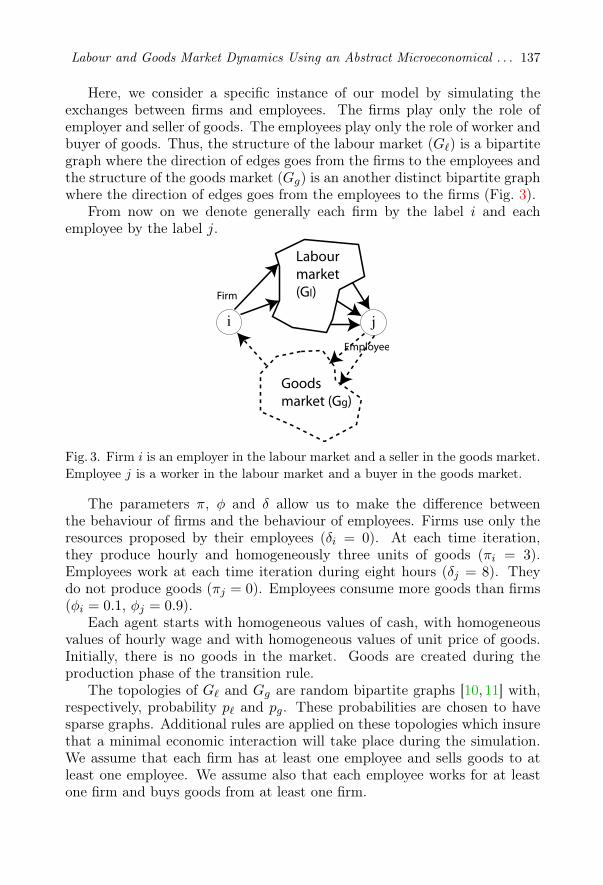
Here, we consider a specific instance of our model by simulating theexchanges between firms and employees. The firms play only the role ofemployer and seller of goods. The employees play only the role of worker andbuyer of goods. Thus, the structure of the labour market (G`) is a bipartitegraph where the direction of edges goes from the firms to the employees andthe structure of the goods market (Gg) is an another distinct bipartite graphwhere the direction of edges goes from the employees to the firms (Fig. 3).

From now on we denote generally each firm by the label i and eachemployee by the label j.

Fig. 3. Firm i is an employer in the labour market and a seller in the goods market.Employee j is a worker in the labour market and a buyer in the goods market.

The parameters π, φ and δ allow us to make the difference betweenthe behaviour of firms and the behaviour of employees. Firms use only theresources proposed by their employees (δi = 0). At each time iteration,they produce hourly and homogeneously three units of goods (πi = 3).Employees work at each time iteration during eight hours (δj = 8). Theydo not produce goods (πj = 0). Employees consume more goods than firms(φi = 0.1, φj = 0.9).

Each agent starts with homogeneous values of cash, with homogeneousvalues of hourly wage and with homogeneous values of unit price of goods.Initially, there is no goods in the market. Goods are created during theproduction phase of the transition rule.

The topologies of G` and Gg are random bipartite graphs [10, 11] with,respectively, probability p` and pg. These probabilities are chosen to havesparse graphs. Additional rules are applied on these topologies which insurethat a minimal economic interaction will take place during the simulation.We assume that each firm has at least one employee and sells goods to atleast one employee. We assume also that each employee works for at leastone firm and buys goods from at least one firm.


4. Results and discussions

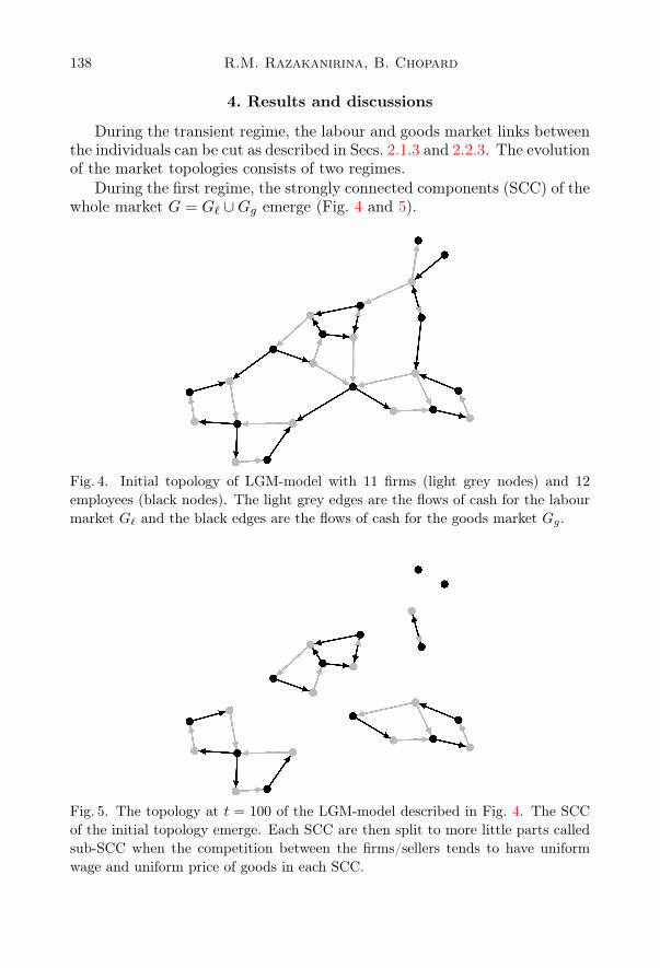
During the transient regime, the labour and goods market links betweenthe individuals can be cut as described in Secs. 2.1.3 and 2.2.3. The evolutionof the market topologies consists of two regimes.

During the first regime, the strongly connected components (SCC) of thewhole market G = G` ∪Gg emerge (Fig. 4 and 5).

Fig. 4. Initial topology of LGM-model with 11 firms (light grey nodes) and 12employees (black nodes). The light grey edges are the flows of cash for the labourmarket G` and the black edges are the flows of cash for the goods market Gg.

Fig. 5. The topology at t = 100 of the LGM-model described in Fig. 4. The SCCof the initial topology emerge. Each SCC are then split to more little parts calledsub-SCC when the competition between the firms/sellers tends to have uniformwage and uniform price of goods in each SCC.


During the second regime, the competition and the cooperation betweenthe cells tend to split the SCC created during the first regime to more littlecomponents that we denote by sub-SCC.

Let us consider an emerging SCC H which consists of firms and employ-ees. Employees cooperate with firms according to the labour links. Em-ployees favour topologically the employer offering the highest hourly wageand the seller proposing the lowest unit price of goods and otherwise therelations. This cooperation creates competition between the firms. The di-vergence of hourly wages and unit price of goods between the firms of Hmeasures the level of competition. If this level is higher than the cuttingedge levels H is split in more little parts. Otherwise, the links between theagents of H are conserved.

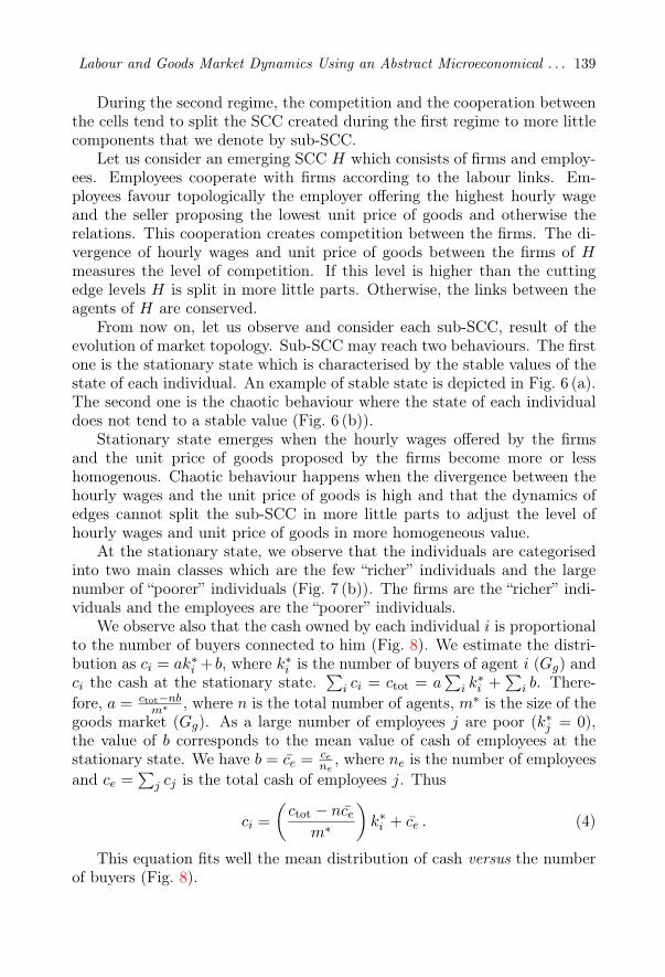
From now on, let us observe and consider each sub-SCC, result of theevolution of market topology. Sub-SCC may reach two behaviours. The firstone is the stationary state which is characterised by the stable values of thestate of each individual. An example of stable state is depicted in Fig. 6 (a).The second one is the chaotic behaviour where the state of each individualdoes not tend to a stable value (Fig. 6 (b)).

Stationary state emerges when the hourly wages offered by the firmsand the unit price of goods proposed by the firms become more or lesshomogenous. Chaotic behaviour happens when the divergence between thehourly wages and the unit price of goods is high and that the dynamics ofedges cannot split the sub-SCC in more little parts to adjust the level ofhourly wages and unit price of goods in more homogeneous value.

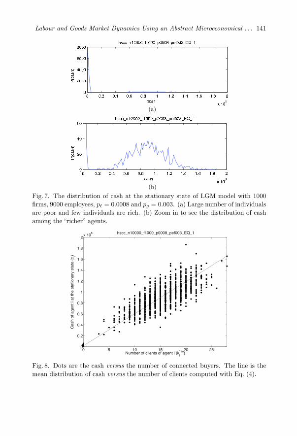
At the stationary state, we observe that the individuals are categorisedinto two main classes which are the few “richer” individuals and the largenumber of “poorer” individuals (Fig. 7 (b)). The firms are the “richer” indi-viduals and the employees are the “poorer” individuals.

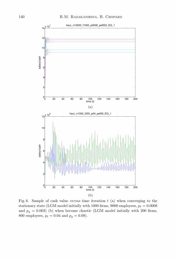
We observe also that the cash owned by each individual i is proportionalto the number of buyers connected to him (Fig. 8). We estimate the distri-bution as ci = ak∗i + b, where k∗i is the number of buyers of agent i (Gg) andci the cash at the stationary state.

∑i ci = ctot = a

∑i k∗i +

∑i b. There-

fore, a = ctot−nbm∗ , where n is the total number of agents, m∗ is the size of the

goods market (Gg). As a large number of employees j are poor (k∗j = 0),the value of b corresponds to the mean value of cash of employees at thestationary state. We have b = c̄e = ce

ne, where ne is the number of employees

and ce =∑

j cj is the total cash of employees j. Thus

ci =(ctot − nc̄e

m∗

)k∗i + c̄e . (4)

This equation fits well the mean distribution of cash versus the numberof buyers (Fig. 8).


0 20 40 60 80 100 120 140 160 180 2000

2

4

6

8

10

12

14x 10

7

time (t)

sa

lary

/ca

sh

hscc_n10000_f1000_p0008_pef003_EQ_1

(a)

0 20 40 60 80 100 120 140 160 180 2000

2

4

6

8

10

12x 10

8

time (t)

sa

lary

/ca

sh

hscc_n1000_f200_p04_pef09_EQ_1

(b)

Fig. 6. Sample of cash value versus time iteration t (a) when converging to thestationary state (LGM model initially with 1000 firms, 9000 employees, p` = 0.0008and pg = 0.003) (b) when become chaotic (LGM model initially with 200 firms,800 employees, p` = 0.04 and pg = 0.09).


(a)

(b)Fig. 7. The distribution of cash at the stationary state of LGM model with 1000firms, 9000 employees, p` = 0.0008 and pg = 0.003. (a) Large number of individualsare poor and few individuals are rich. (b) Zoom in to see the distribution of cashamong the “richer” agents.

0 5 10 15 20 250

0.2

0.4

0.6

0.8

1

1.2

1.4

1.6

1.8

2x 10

8

Number of clients of agent i (ki

* in)

Ca

sh

of a

ge

nt i a

t th

e s

tatio

na

ry s

tate

(c

i)

hscc_n10000_f1000_p0008_pef003_EQ_1

Fig. 8. Dots are the cash versus the number of connected buyers. The line is themean distribution of cash versus the number of clients computed with Eq. (4).


One can calculate numerically the distribution of cash when the hourlywages become uniform and the unit prices of goods become uniform. Thevalues of cash are obtained by solving the following system of linear equationsexpressing the rule of the model (the details of the calculations are givenin [12])

λcj = (1− λ)γ∑∀m

ψmjcm , where ψij =

aij

kinj∑∀`

ai`

kin`

, (5)

ci =∑∀k

∑∀m

θkiψmkcm , where θij =bijk∗outi

, (6)

ctot =∑

i(firms)

ci +∑

j(employees)

cj , (7)

where i and j denote respectively the labels of firms and the labels of em-ployees. With LGM model, cash value is a centrality measure qualifying theweight of each individual in the whole network. As described above, thenumber of buyers connected with the individual impacts on the distributionof cash. We show that the mean distribution of cash (Eq. (4)) is closelyrelated to the so-called page rank of each individual.

5. Conclusion and future work

We have studied the behaviours of a particular multilayer cellular au-tomata on a graph (MCAG) denoted LGM model which models the labourand goods market dynamics. This model merges the hour against salary/cashdynamics (labour market) and the cash against goods dynamics (goods mar-ket). The topologies of labour and goods markets are distinct making theMCAG formalism useful.

We found that the SCC of the labour and goods market taken togetheremerge. Each SCC tends to be split in more little subcomponents depend-ing on the level of competition between the firms in the SCC. This levelis determined by the divergence of hourly wage and unit prices of goodsbetween the firms. This competition impacts also the final state of the sub-components which may be stationary or may be chaotic. Chaotic behaviourappeared when competition takes place but cannot split the SCC in morelittle subcomponents. The steady state emerge when the wages and theunit prices of goods proposed by the firms become homogeneous, allowing aperfect competition between the firms in each SCC.


Considering each subcomponent at the stationary state, two main classesof cells emerge which are the richer cells and the poorer cells. The richerones are the employers and the poorer ones are the workers. We found alsothat the distribution of the amount of cash is proportional to the number ofthe buyers of the cell.

As an extension, firms could buy goods from other firms or work forthem, thus modelling more levels of commercial relationship between them.

We acknowledge financial support from the Swiss National Science Foun-dation.

REFERENCES

[1] R.M. Razakanirina, B. Chopard, Multilayer Cellular Automata on a GraphApplied to the Exchanges of Cash and Goods, Journal of Cellular Automata,OCP Science, 2011 (in press).

[2] J.B. Glattfelder, “Ownership Networks and Corporate Control: MappingEconomic Power in a Globalized World”, PhD thesis, ETH Zurich,Department of Management, Technology, and Economics, 2010.

[3] C.S. Wagner, L. Leydesdorff, Research Policy 34, 1608 (2005).[4] G. Caldarelli, Scale-Free Networks: Complex Webs in Nature and Technology

(Oxford Finance), Oxford University Press, USA, 2007.[5] M. Serrano, M. Boguñá, A. Vespignani, Journal of Economic Interaction and

Coordination 2, 111 (2007).[6] R. Albert, A.-L. Barabási, Phys. Rev. Lett. 85, 5234 (2000).[7] A. Hoekstra, J. Kroc, P. Sloot, Modelling Complex Systems with Cellular

Automata, Springer-Verlag, 2010.[8] R.M. Razakanirina, B. Chopard, Using Cellular Automata on a Graph to

Model the Exchanges of Cash and Goods, ACRI proceedings, pp. 163–172,2010.

[9] S.S. Epp, Discrete Mathematics with Applications, Richard Stratton, 2011.[10] R.D. Richard Durrett, M. Stein, Random Graph Dynamics, Cambridge

University Press, 1 edition, 2010.[11] S.N. Dorogovtsev, J.F.F. Mendes, A.N. Samukhin, Phys. Rev. E64, 025101

(2001).[12] R.M. Razakanirina, B. Chopard, “Hour and Salary Complex Model at the

Steady State: Detailed Analytical Calculations”, 2011,http://www.ambohimalaza.org/phd/hsc/hscsteadystate.pdf

http://dx.doi.org/10.1016/j.respol.2005.08.002

http://dx.doi.org/10.1103/PhysRevLett.85.5234

http://dx.doi.org/10.1103/PhysRevE.64.025101

http://dx.doi.org/10.1103/PhysRevE.64.025101

LABOUR AND GOODS MARKET DYNAMICS USING AN ABSTRACT MICROECONOMICAL MODEL

Documents