This article appeared in a journal published by Elsevier. The attached copy is furnished to the author for internal non-commercial research and education use, including for instruction at the authors institution and sharing with colleagues. Other uses, including reproduction and distribution, or selling or licensing copies, or posting to personal, institutional or third party websites are prohibited. In most cases authors are permitted to post their version of the article (e.g. in Word or Tex form) to their personal website or institutional repository. Authors requiring further information regarding Elsevier’s archiving and manuscript policies are encouraged to visit: http://www.elsevier.com/copyright

Welcome message from author
This document is posted to help you gain knowledge. Please leave a comment to let me know what you think about it! Share it to your friends and learn new things together.
Transcript

This article appeared in a journal published by Elsevier. The attachedcopy is furnished to the author for internal non-commercial researchand education use, including for instruction at the authors institution
and sharing with colleagues.
Other uses, including reproduction and distribution, or selling orlicensing copies, or posting to personal, institutional or third party
websites are prohibited.
In most cases authors are permitted to post their version of thearticle (e.g. in Word or Tex form) to their personal website orinstitutional repository. Authors requiring further information
regarding Elsevier’s archiving and manuscript policies areencouraged to visit:
http://www.elsevier.com/copyright
Author's personal copy
Journal of Multivariate Analysis 104 (2012) 159–173
Contents lists available at SciVerse ScienceDirect
Journal of Multivariate Analysis
journal homepage: www.elsevier.com/locate/jmva
Relational models for contingency tablesAnna Klimova a,∗, Tamás Rudas b, Adrian Dobra c
a Department of Statistics, University of Washington, Box 355845, Seattle, WA 98195-4322, USAb Department of Statistics, Eötvös Loránd University, Pazmany Peter setany 1/A, H-1117, Budapest, Hungaryc Department of Statistics, University of Washington, Box 354322, Seattle, WA 98195-4322, USA
a r t i c l e i n f o
Article history:Received 9 March 2011Available online 23 July 2011
AMS subject classifications:62J1262B0562P25
Keywords:Contingency tablesCurved exponential familyExponential familyGeneralized odds ratiosMaximum likelihood estimateMultiplicative model
a b s t r a c t
The paper considers general multiplicative models for complete and incompletecontingency tables that generalize log-linear and several other models and are entirelycoordinate free. Sufficient conditions for the existence of maximum likelihood estimatesunder these models are given, and it is shown that the usual equivalence betweenmultinomial and Poisson likelihoods holds if and only if an overall effect is present in themodel. If such an effect is not assumed, the model becomes a curved exponential familyand a relatedmixed parameterization is given that relies on non-homogeneous odds ratios.Several examples are presented to illustrate the properties and use of such models.
© 2011 Elsevier Inc. All rights reserved.
0. Introduction
The main objective of the paper is to develop a new class of models for the set of all strictly positive distributionson contingency tables and on some sets of cells that have a more general structure. The proposed relational models aremotivated by traditional log-linear models, quasi models, and some other multiplicative models for discrete distributionsthat have been discussed in the literature.
Under log-linear models [7], cell probabilities are determined by multiplicative effects associated with varioussubsets of the variables in the contingency table. However, some cells may have other characteristics in common,and there always has been interest in models that also allow for multiplicative effects that are associated with thosecharacteristics. Examples, among others, include quasi models [13,14], topological models [16,18], indicator models [29],rater agreement–disagreement models [26,27], two-way subtable sum models [15]. All these models, applied in differentcontexts, have one common idea behind them. A model is generated by a class of subsets of cells, some of which may notbe induced by marginals of the table, and, under the model, every cell probability is the product of effects associated withsubsets the cell belongs to. This idea is generalized in the relational model framework.
The outline of the paper is as follows. The definition of a table and the definition of a relational model generated bya class of subsets of cells in the table are given in Section 1. The cells are characterized by strictly positive parameters(probabilities or intensities); a table is a structured set of cells. Under the model, the parameter of each cell is the productof effects associated with the subsets in the generating class, to which the cell belongs. Two examples are given to illustrate
∗ Corresponding author.E-mail addresses: [email protected] (A. Klimova), [email protected] (T. Rudas), [email protected] (A. Dobra).
0047-259X/$ – see front matter© 2011 Elsevier Inc. All rights reserved.doi:10.1016/j.jmva.2011.07.006
Author's personal copy
160 A. Klimova et al. / Journal of Multivariate Analysis 104 (2012) 159–173
this definition. Example 1.1 shows how traditional log-linear models fit into the framework, and Example 1.2 describes howmultiplicative models for incomplete contingency tables are handled.
The degrees of freedom and the dual representation of relational models are discussed in Section 2. Every relationalmodel can be stated in terms of generalized odds ratios. The minimal number of generalized odds ratios required to specifythe model is equal to the number of degrees of freedom of this model.
Themodels for probabilities that include the overall effect and all relationalmodels for intensities are regular exponentialfamilies. Under known conditions (cf. [3]), the maximum likelihood estimates for cell frequencies exist and are unique; themean-value parameters of the MLE, associated with the subsets of the model, are equal to the corresponding mean-valueparameters of the observeddistribution. Themaximum likelihood estimates for cell frequencies under amodel for intensitiesand under a model for probabilities, when the model matrix is the same, are equal if and only if the model for probabilitiesis a regular family. These facts are proven in Section 3.
The main results of the paper, given in Section 4, discuss the properties of the MLE under relational models without theoverall effect. If the overall effect is not present, a relational model for probabilities forms a curved exponential family. Themaximum likelihood estimates in the curved case exist and are unique under the same condition as for regular families. Forany relational model, the mean-value parameters of the MLE, associated with the subsets of the model, are proportional tothe corresponding mean-value parameters of the observed distribution. The parameter space and the relational models arealso described in terms of algebraic geometry.
A mixed parameterization of finite discrete exponential families is discussed in Section 5. Any relational model isnaturally defined under this parameterization: the corresponding generalized odds ratios are fixed and the model isparameterized by remaining mean-value parameters. The distributions of observed values of subset sums and generalizedodds ratios are variation independent and, in the regular case, specify the table uniquely.
Two applications of the framework are presented in Section 6. These are analyses of social mobility data and of avalued network with given attributes. These two examples suggest that the flexibility of the framework and substantiveinterpretations of parameters make relational models appealing in many settings.
1. Definition and log-linear representation of relational models
Let Y1, . . . , YK be the discrete random variables modeling certain characteristics of the population of interest. Denote thedomains of the variables by Y1, . . . ,YK respectively. A point (y1, y2, . . . , yK ) ∈ Y1 × · · · × YK generates a cell if and onlyif the outcome (y1, y2, . . . , yK ) appears in the population. A cell (y1, y2, . . . , yK ) is called empty if the combination is notincluded in the design.
Let I denote the lexicographically ordered set of non-empty cells in Y1 × · · · × YK , and |I| denote the cardinality of I.Since the case, when I = Y1 × · · · × YK , corresponds to a classical complete contingency table, then the set I is also calleda table.
Depending on the procedure that generates data on I, the population may be characterized by cell probabilities or cellintensities. The parameters of the true distribution will be denoted by δ = δ(i), for i ∈ I. In the case of probabilities,δ(i) = p(i) ∈ (0, 1), where
∑i∈I p(i) = 1; in the case of intensities, δ(i) = λ(i) > 0.
Write P = Pδ : δ ∈ Ω for the set of all positive distributions on the table I. Here the parameter space Ω is an opensubset of R|I|. Suppose Θ ⊂ Ω . Then the set PΘ = Pδ ∈ P : δ ∈ Θ is a model in P .
Definition 1.1. Let S = S1, . . . , SJ be a class of non-empty subsets of the table I and A be a J × |I| matrix with entries
aji = Ij(i) =
1, if the i-th cell is in Sj,0, otherwise, for i = 1, . . . , |I| and j = 1, . . . , J. (1)
A relational model RM(S) with the model matrix A is the following subset of P:
RM(S) = Pδ ∈ P : log δ = A′β, for some β ∈ RJ. (2)
Under the model (2) the parameters of the distribution can also be written as
δ(i) = exp
J−
j=1
Ij(i)βj
=
J∏j=1
(θj)Ij(i), (3)
where θj = exp(βj), for j = 1, . . . , J .The parameters β in (2) are called the log-linear parameters. The parameters θ in (3) are called the multiplicative
parameters. If the subsets in S are cylinder sets, the parameters β coincide with the parameters of the corresponding log-linear model.
In the case δ = p it must be assumed that ∪Jj=1 Sj = I, i.e. there are no zero columns in the matrix A. A zero column
implies that one of the probabilities is 1 under the model and the model is thus trivial.The example below describes a model of conditional independence as a relational model.

Author's personal copy
A. Klimova et al. / Journal of Multivariate Analysis 104 (2012) 159–173 161
Table 1Poisson intensities by bait type.
Sugarcane FishYes No
Yes λ00 λ01No λ10 –
Example 1.1. Consider the model of conditional independence [Y1Y3][Y2Y3] of three binary variables Y1, Y2, Y3, each takingvalues in 0, 1. The model is expressed as
pijk =pi+kp+jk
p++k,
where pi+k, p+jk, p++k are marginal probabilities in the standard notation [7]. Let S be the class consisting of the cylindersets associated with the empty marginal and with the marginals Y1, Y2, Y3, Y1Y3, Y2Y3. The model matrix computed from (1)is not full row rank and thus the model parameters are not identifiable (cf. Section 2). A full row rank model matrix can beobtained by setting, for instance, the level 0 of each variable as the reference level. After that, the model matrix is equal to
A =
1 1 1 1 1 1 1 10 0 0 0 1 1 1 10 0 1 1 0 0 1 10 1 0 1 0 1 0 10 0 0 0 0 1 0 10 0 0 1 0 0 0 1
. (4)
The first row corresponds to the cylinder set associated with the empty marginal. The next three rows correspond to thecylinder sets generated by the level 1 of Y1, Y2, Y3 respectively. The fifth row corresponds to the cylinder set generated bythe level 1 for both Y1 and Y3, and the last row—to the cylinder set corresponding to the level 1 for both Y2 and Y3.
In the next example, one of the cells in the Cartesian product of the domains of the variables is empty and the samplespace I is a proper subset of this product.
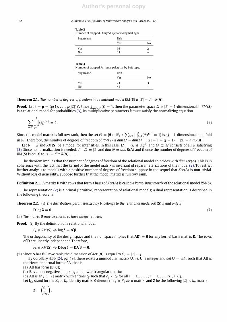
Example 1.2. The study described by Kawamura et al. [20] compared three bait types for trapping swimming crabs: fishalone, sugarcane alone, and sugarcane–fish combination. The observed frequencies are given in Tables 2 and 3. During theexperiment, catching crabs without bait was not considered. Three Poisson random variables are used to model the amountof crabs caught in the three traps. The notation for the intensities is shown in Table 1. The model assuming that there is amultiplicative effect of using both bait types at the same time will be tested in this paper. The hypothesis of interest is
λ00 = λ01λ10. (5)
The effect can be tested using the relational model for intensities on the class S consisting of two subsets—S = S1, S2,where S1 = (0, 0), (0, 1) and S2 = (0, 0), (1, 0):
logλ = A′β.
Here, the model matrix is
A =
1 1 01 0 1
,
and β = (β1, β2)′. The relationship between the two forms of the model will be explored in the next section.
2. Parameterizations and degrees of freedom
A choice of subsets in S = S1, . . . , SJ is implied by the statistical problem, and the relational model RM(S) canbe parameterized with different model matrices, which may be useful depending on substantive meaning of the model.Sometimes a particular choice of subsets leads to a model matrix Awith linearly dependent rows and thus non-identifiablemodel parameters. To ensure identifiability, a reparameterization, that is sometimes referred to as model matrix coding,is needed. Examples of frequently used codings are reference coding, effect coding, orthogonal coding, polynomial coding(cf. [10]).
Write R(A) for the row space of A and call it the design space of the model. The elements of R(A) are |I|-dimensionalrow-vectors and 1 denotes the row-vector with all components equal to 1. Reparameterizations of the model have formβ = Cβ1, where β1 are the new parameters of themodel and C is a J ×[rank(A)]matrix such that themodifiedmodel matrixC′A has full row rank and R(A) = R(C′A). Then R(A)⊥ = R(C′A)⊥, that is Ker(A) = Ker(C′A).
Of course, the reparameterization does not affect the number of degrees of freedom. The number of degrees of freedomof a model PΘ ⊂ P is the difference between dimensionalities of Ω and Θ .
Author's personal copy
162 A. Klimova et al. / Journal of Multivariate Analysis 104 (2012) 159–173
Table 2Number of trapped Charybdis japonica by bait type.
Sugarcane FishYes No
Yes 36 2No 11 –
Table 3Number of trapped Portunus pelagicus by bait type.
Sugarcane FishYes No
Yes 71 3No 44 –
Theorem 2.1. The number of degrees of freedom in a relational model RM(S) is |I| − dim R(A).
Proof. Let δ = p = (p(1), . . . , p(|I|))′. Since∑
i∈I p(i) = 1, then the parameter space Ω is |I| − 1-dimensional. If RM(S)is a relational model for probabilities (3), its multiplicative parameters θ must satisfy the normalizing equation
−i∈I
J∏j=1
(θj)Ij(i) = 1. (6)
Since themodel matrix is full row rank, then the setΘ = θ ∈ RJ+ :
∑i∈I∏J
j=1(θj)Ij(i) = 1 is a J −1-dimensional manifold
in RJ . Therefore, the number of degrees of freedom of RM(S) is dimΩ − dimΘ = |I| − 1 − (J − 1) = |I| − dimR(A).Let δ = λ and RM(S) be a model for intensities. In this case, Ω = λ ∈ R|I|
+ and Θ ⊂ Ω consists of all λ satisfying(3). Since no normalization is needed, dimΩ = |I| and dimΘ = dim R(A) and thence the number of degrees of freedom ofRM(S) is equal to |I| − dim R(A).
The theorem implies that the number of degrees of freedom of the relational model coincides with dim Ker(A). This is incoherence with the fact that the kernel of the model matrix is invariant of reparameterizations of the model (2). To restrictfurther analysis to models with a positive number of degrees of freedom suppose in the sequel that Ker(A) is non-trivial.Without loss of generality, suppose further that the model matrix is full row rank.
Definition 2.1. AmatrixDwith rows that form a basis of Ker(A) is called a kernel basis matrix of the relational model RM(S).
The representation (2) is a primal (intuitive) representation of relational models; a dual representation is described inthe following theorem.
Theorem 2.2. (i) The distribution, parameterized by δ, belongs to the relational model RM(S) if and only if
D log δ = 0. (7)
(ii) The matrix D may be chosen to have integer entries.
Proof. (i) By the definition of a relational model,
Pδ ∈ RM(S) ⇔ log δ = A′β.
The orthogonality of the design space and the null space implies that AD′= 0 for any kernel basis matrix D. The rows
of D are linearly independent. Therefore,
Pδ ∈ RM(S) ⇔ D log δ = DA′β = 0.
(ii) Since A has full row rank, the dimension of Ker (A) is equal to K0 = |I| − J .By Corollary 4.3b [24, pg. 49], there exists a unimodular matrix U, i.e. U is integer and det U = ±1, such that AU is
the Hermite normal form of A, that is(a) AU has form [B, 0];(b) B is a non-negative, non-singular, lower triangular matrix;(c) AU is an J × |I| matrix with entries cij such that cij < cii for all i = 1, . . . , J, j = 1, . . . , |I|, i = j.Let IK0 stand for the K0 × K0 identity matrix, 0 denote the J × K0 zero matrix, and Z be the following |I| × K0 matrix:
Z =
0IK0
.

Author's personal copy
A. Klimova et al. / Journal of Multivariate Analysis 104 (2012) 159–173 163
Since the matrix AU has form [B, 0], where B is the nonsingular, lower triangular, J × J matrix, then (AU)Z = 0.Set D′
= UZ. Then
AD′= AUZ = 0. (8)
The matrix U is integer and nonsingular, the columns of Z are linearly independent. Therefore, the matrix D′ is integerand has linearly independent columns. Hence the matrix D is an integer kernel basis matrix of the model.
Example 1.1 (Revisited). For the model of conditional independence, dim Ker(A) = 2. If the kernel basis matrix is chosen as
D =
1 0 −1 0 −1 0 1 00 1 0 −1 0 −1 0 1
,
the equation D log p = 0 is equivalent to the following constraints:p000p110p010p100
= 1,p001p111p011p101
= 1.
The latter is a well-known representation of the model [Y1Y3][Y2Y3] in terms of the conditional odds ratios [7].
The dual representation (7) of a relational model is, in fact, a model representation in terms of some monomials in δ. Alltypes of polynomial expressions thatmay arise in the dual representation of a relationalmodel are captured by the followingdefinition.
Definition 2.2. Let u(i), v(i) ∈ Z≥0 for all i ∈ I, δu=∏
i∈I δ(i)u(i) and δv=∏
i∈I δ(i)v(i). A generalized odds ratio for apositive distribution, parameterized by δ, is a ratio of two monomials:
OR = δu/δv. (9)
The odds ratio OR = δu/δv is called homogeneous if∑
i∈I u(i) =∑
i∈I v(i).To express a relational model RM(S) in terms of generalized odds ratios, write the rows d1, d2, . . . , dK0 ∈ Z|I| of a kernel
basis matrix D in terms of their positive and negative parts:
dl = d+
l − d−
l ,
where d+
l , d−
l ≥ 0 for all l = 1, 2, . . . , K0. Then the model (7) takes the form
d+
l log δ = d−
l log δ, for l = 1, 2, . . . , K0,
which is equivalent to the model representation in terms of generalized odds ratios:
δd+
l /δd−
l = 1, for l = 1, 2, . . . , K0. (10)
The number of degrees of freedom is equal to the minimal number of generalized odds ratios required to uniquely specifya relational model.
Example 1.2 (Revisited). The model λ00 = λ01λ10 can be expressed in the matrix form as
D logλ = 0, (11)
where D = (1, −1, −1). The matrix D is a kernel basis matrix of the relational model, as one would expect. Finally, themodel representation in terms of generalized odds ratios is
λ00
λ01λ10= 1.
The role of generalized odds ratios in parameterizing distributions in P will be explored in Section 5.
3. Relational models as exponential families: Poisson vs multinomial sampling
The representation (3) implies that a relational model is an exponential family of distributions. The canonical parametersof a relational model are βj’s and the canonical statistics are indicators of subsets Ij. Relational models for intensities andrelational models for probabilities are considered in this section in more detail.
Let RMλ(S) denote a relationalmodel for intensities and RMp(S) denote a relationalmodel for probabilities with the samemodel matrix A, that has a full row rank J .
Theorem 3.1. A model RMλ(S) is a regular exponential family of order J .

Author's personal copy
164 A. Klimova et al. / Journal of Multivariate Analysis 104 (2012) 159–173
Proof. Themodel matrix A in (2) has full row rank; no normalization is needed for intensities. Therefore, the representation(3) is minimal and the exponential family is regular, of order J .
Relational models for probabilities may have a more complex structure than relational models for intensities and, insome cases, become curved exponential families [12,9,19].
Theorem 3.2. If 1 ∈ R(A), a model RMp(S) is a regular exponential family of order J − 1; otherwise, it is a curved exponentialfamily of order J − 1.
Proof. Suppose that 1 ∈ R(A). Without loss of generality, I = S1 ∈ S and thus
p(i) = expβ1 exp
J−
j=2
Ij(i)βj
. (12)
The exponential family representation given by (12) is minimal; the model RMp(S) is a regular exponential family of orderJ − 1.
If 1 ∈ R(A) then, independently of what parameterization is used, the model matrix does not include the row of all 1s.Then normalization is required and thus the parameter space is a manifold of dimension J − 1 in RJ (see e.g. [23], p. 229). Inthis case, RMp(S) is a curved exponential family of order J − 1 [19].
If a relational model is a regular exponential family, the maximum likelihood estimate of the canonical parameter existsif and only if the observed value of the canonical statistic is contained in the interior of the convex hull of the support of itsdistribution [3]. In this case, the MLE is also unique.
If the distribution of a random vector Y is parameterized by intensities λ, then, under the model RMλ(S),
P(Y = y) =1∏
i∈Iy(i)!
expβ′Ay − 1 expA′β. (13)
If the distribution of Y is multinomial, with parameters N and p, then, under the model RMp(S),
P(Y = y) =N!∏
i∈Iy(i)!
expβ′Ay. (14)
Set
T (Y) = AY = (T1(Y), T2(Y), . . . , TJ(Y))′. (15)
For each j ∈ 1, . . . , J , the statistic Tj(Y) =∑
i∈I Ij(i)Y (i) is the subset sum corresponding to the subset Sj.It is well known for log-linear models that the kernel of the likelihood is the same for the multinomial and Poisson
sampling schemes, if the sample sizes are equal, and thus themaximum likelihood estimates of the cell frequencies, obtainedunder either sampling scheme, are equal (see e.g. [6], [7, p. 448]). The following theorem is an extension of this result.
Theorem 3.3. Assume that, for a given set of observations, the maximum likelihood estimates λ, under the model RMλ(S), and p,under the model RMp(S), exist. The following four conditions are equivalent:
(A) The MLEs for the cell frequencies obtained under either model are the same.(B) The vector 1 is in the design space R(A).(C) Both models may be defined by homogeneous odds ratios.(D) The model for intensities is scale invariant.
Proof. (A) ⇐H (B)Under the model RMp(S), the probabilities can be written in the form (3):
p(i) =
J∏j=1
(θj)Ij(i), i ∈ I,
where βj = log θj, for j = 1, . . . , J . The problem of maximization, with respect to θ, of the likelihood (14) under thenormalization condition (6) is equivalent to maximizing the Lagrangian
L(θ) =
−i∈I
y(i)J−
j=1
Ij(i) log θj − α
−i∈I
J∏j=1
(θj)Ij(i) − 1
.
Author's personal copy
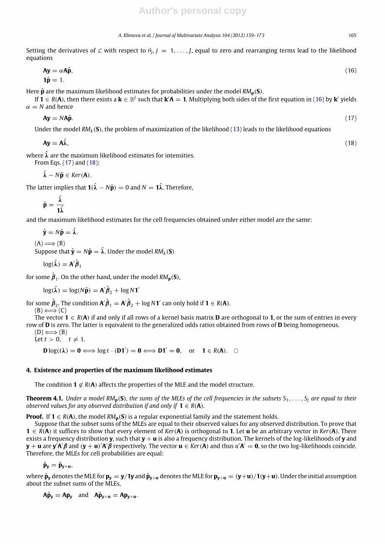
A. Klimova et al. / Journal of Multivariate Analysis 104 (2012) 159–173 165
Setting the derivatives of L with respect to θj, j = 1, . . . , J , equal to zero and rearranging terms lead to the likelihoodequations
Ay = αAp, (16)1p = 1.
Here p are the maximum likelihood estimates for probabilities under the model RMp(S).If 1 ∈ R(A), then there exists a k ∈ RJ such that k′A = 1. Multiplying both sides of the first equation in (16) by k′ yields
α = N and hence
Ay = NAp. (17)
Under the model RMλ(S), the problem of maximization of the likelihood (13) leads to the likelihood equations
Ay = Aλ, (18)
where λ are the maximum likelihood estimates for intensities.From Eqs. (17) and (18):
λ − Np ∈ Ker(A).
The latter implies that 1(λ − Np) = 0 and N = 1λ. Therefore,
p =λ
1λand the maximum likelihood estimates for the cell frequencies obtained under either model are the same:
y = Np = λ.
(A) H⇒ (B)Suppose that y = Np = λ. Under the model RMλ(S)
log(λ) = A′β1
for some β1. On the other hand, under the model RMp(S),
log(λ) = log(Np) = A′β2 + logN1′
for some β2. The condition A′β1 = A′β2 + logN1′ can only hold if 1 ∈ R(A).(B) ⇐⇒ (C)The vector 1 ∈ R(A) if and only if all rows of a kernel basis matrix D are orthogonal to 1, or the sum of entries in every
row of D is zero. The latter is equivalent to the generalized odds ratios obtained from rows of D being homogeneous.(D) ⇐⇒ (B)Let t > 0, t = 1.
D log(tλ) = 0 ⇐⇒ log t · (D1′) = 0 ⇐⇒ D1′= 0, or 1 ∈ R(A).
4. Existence and properties of the maximum likelihood estimates
The condition 1 ∈ R(A) affects the properties of the MLE and the model structure.
Theorem 4.1. Under a model RMp(S), the sums of the MLEs of the cell frequencies in the subsets S1, . . . , SJ are equal to theirobserved values for any observed distribution if and only if 1 ∈ R(A).
Proof. If 1 ∈ R(A), the model RMp(S) is a regular exponential family and the statement holds.Suppose that the subset sums of the MLEs are equal to their observed values for any observed distribution. To prove that
1 ∈ R(A) it suffices to show that every element of Ker(A) is orthogonal to 1. Let u be an arbitrary vector in Ker(A). Thereexists a frequency distribution y, such that y + u is also a frequency distribution. The kernels of the log-likelihoods of y andy + u are y′A′β and (y + u)′A′β respectively. The vector u ∈ Ker(A) and thus u′A′
= 0, so the two log-likelihoods coincide.Therefore, the MLEs for cell probabilities are equal:
py = py+u,
where py denotes theMLE forpy = y/1y and py+u denotes theMLE forpy+u = (y+u)/1(y+u). Under the initial assumptionabout the subset sums of the MLEs,
Apy = Apy and Apy+u = Apy+u.

Author's personal copy
166 A. Klimova et al. / Journal of Multivariate Analysis 104 (2012) 159–173
Therefore, using that Au = 0,
Ay1y
= Apy = Apy+u = Ay + u
1(y + u)= A
y1(y + u)
,
implying the equality 1y = 1(y + u), which is possible if and only if 1u = 0.
Corollary 4.2. Suppose 1 ∈ R(A). For a given set of observations, the MLEs, if exist, of the subset sums under a model RMp(S) areproportional to their observed values.
Proof. In this case the value of α cannot be found from (16) and one can only assert that
Ay =α
NAy.
Example 1.2 illustrates a situation when a relational model for intensities is not scale invariant. This model is a curvedexponential family. The existence and uniqueness of themaximum likelihood estimates in such relationalmodels are provennext.
Theorem 4.3. Let Y ∼ M (N, p), y be a realization of Y, and RMp(S) be a relational model, such that 1 ∈ R(A). The maximumlikelihood estimate for p, under the model RMp(S), exists and is unique if and only if T (y) > 0.
Proof. A point in the canonical parameter space of the model RMp(S) that maximizes the log-likelihood subject to thenormalization constraint is a solution to the optimization problem:
max l(β; y),s.t. β∈D
where
l(β; y) = T1(y)β1 + · · · + TJ(y)βJ
and
D =
β ∈ RJ
− :
−i∈I
exp
J−
j=1
Ij(i)βj
− 1 = 0
.
The set D is non-empty and is a level set of a convex function. The level sets of convex functions are not convex in general.However, the sub-level sets of convex functions and hence the set
D≤ =
β ∈ RJ
− :
−i∈I
exp
J−
j=1
Ij(i)βj
− 1 ≤ 0
are convex.
The set of maxima of l(β; y) over the set D≤ is nonempty and consists of a single point if and only if [5, Section 3]
RD≤∩ R−l = LD≤
∩ L−l.
Here RD≤is the recession cone of the set D≤, R−l is the recession cone of the function −l, LD≤
is the lineality space of D≤,and L−l is the lineality space of −l.
The recession cone of D≤ is the orthant RJ−, including the origin; the lineality space is LD≤
= 0. The lineality spaceof the function −l is the plane passing through the origin, with the normal T(y); the recession cone of −l is the half-spaceabove this plane. The condition RD≤
∩R−l = LD≤∩L−l = 0 holds if and only if all components of T(y) = (T1(y), . . . , TJ(y))′
are positive.The function l(β; y) is linear; its maximum is achieved onD. Therefore, there exists one and only one βwhichmaximizes
the likelihood over the canonical parameter space, and the maximum likelihood estimate for p, under the model RMp(S),exists and is unique.

Author's personal copy
A. Klimova et al. / Journal of Multivariate Analysis 104 (2012) 159–173 167
Table 4The MLEs for the number of trappedCharybdis japonica by bait type.
Sugarcane FishYes No
Yes 35.06 2.94No 11.94 –
Table 5The MLEs for the number of trappedPortunus pelagicus by bait type.
Sugarcane FishYes No
Yes 72.31 1.69No 42.69 –
Example 1.2 (Revisited). In this example, the relational model for intensities is not scale invariant. Themaximum likelihoodestimates for the cell frequencies exist and are shown in Tables 4 and 5. The observed Pearson’s statistics are X2
= 0.40 andX2
= 1.07 respectively, on one degree of freedom.
The relational model framework deals with models generated by subsets of cells, and the model matrix for a relationalmodel is an indicator matrix that has only 0–1 entries. Theorems 2.2 and 3.3 hold if the model matrix has non-negativeinteger entries. The next example illustrates how the techniques and theorems apply to those more general exponentialfamilies.
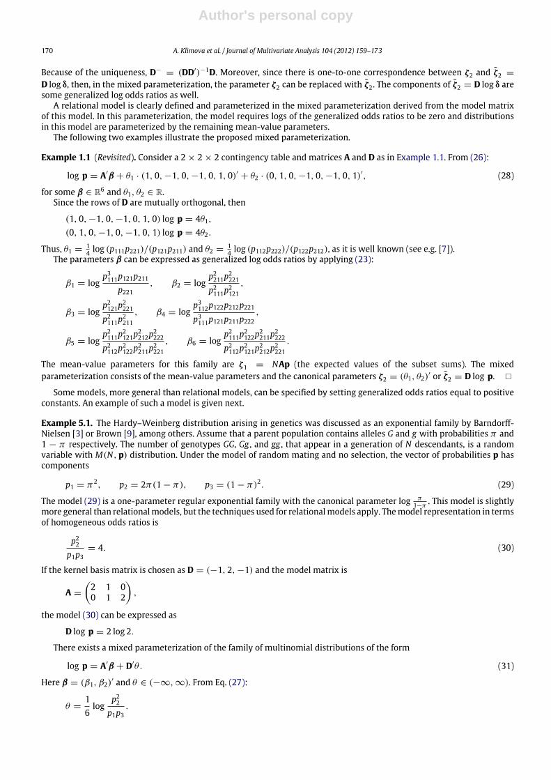
Example 4.1. This example, given in [1], describes a study carried out to determine if a pneumonia infection has animmunizing effect on dairy calves. Within 60 days after birth, the calves were exposed to a pneumonia infection. Thecalves that got the infection were then classified according to whether or not they got the secondary infection within twoweeks after the first infection cleared up. The number of the infected calves is thus a random variable with the multinomialdistributionM(N, (p11, p12, p22)′), where N denotes the total number of calves in the sample. Suppose further that p11 is theprobability to get both the primary and the secondary infection, p12 is the probability to get only the primary infection andnot the secondary one, and p22 is the probability not to catch either the primary or the secondary infection. Let 0 < π < 1denote the probability to get the primary infection. The hypothesis of no immunizing effect of the primary infection isexpressed as (cf. [1])
p11 = π2, p12 = π(1 − π), p22 = 1 − π. (19)
Themodel given in (19) does not contain the overall effect and can be expressed in terms of a non-homogeneous odds ratio:
p11p222p212
= 1.
Write N11,N12,N22 for the number of calves, as a random variable in each category, and n11, n12, n22 for their realizations.The log-likelihood is proportional to
(2n11 + n12) log π + (n12 + n22) log (1 − π).
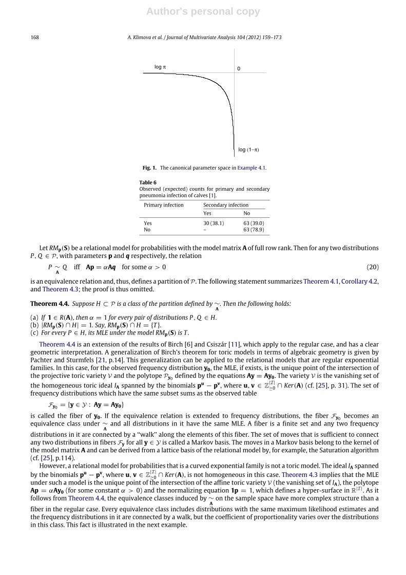
The sufficient statistic T = (2N11+N12,N12+N22) is two-dimensional. The canonical parameter space (logπ, log(1−π)) :
π ∈ (0, 1) is the curve in R2 shown in Fig. 1. The model (19) is thus a curved exponential family of order 1.The likelihood is maximized by
π =2n11 + n12
2n11 + 2n12 + n22=
T1T1 + T2
,
where T1 = 2n11 + n12 and T2 = n12 + n22 are the observed components of the sufficient statistic, or the subset sums. TheMLEs of the subset sums can be expressed in terms of their observed values as
N(2π2+ π(1 − π)) = N
2T 2
1
(T1 + T2)2+
T1T2(T1 + T2)2
= T1
N(2T1 + T2)(T1 + T2)2
,
N(π(1 − π) + (1 − π)) = N
T1T2(T1 + T2)2
+T2
T1 + T2
= T2
N(2T1 + T2)(T1 + T2)2
.
Thus, under the model (19), the MLEs of the subset sums differ from their observed values by the factor N(2T1+T2)(T1+T2)2
. For thedata and the MLEs in Table 6, this factor is approximately 0.936.
Author's personal copy
168 A. Klimova et al. / Journal of Multivariate Analysis 104 (2012) 159–173
log π
log (1−π)
0
Fig. 1. The canonical parameter space in Example 4.1.
Table 6Observed (expected) counts for primary and secondarypneumonia infection of calves [1].
Primary infection Secondary infectionYes No
Yes 30 (38.1) 63 (39.0)No – 63 (78.9)
Let RMp(S) be a relationalmodel for probabilities with themodelmatrixA of full row rank. Then for any two distributionsP,Q ∈ P , with parameters p and q respectively, the relation
P ∼A
Q iff Ap = αAq for some α > 0 (20)
is an equivalence relation and, thus, defines a partition ofP . The following statement summarizes Theorem4.1, Corollary 4.2,and Theorem 4.3; the proof is thus omitted.
Theorem 4.4. Suppose H ⊂ P is a class of the partition defined by ∼A. Then the following holds:
(a) If 1 ∈ R(A), then α = 1 for every pair of distributions P,Q ∈ H.(b) |RMp(S) ∩ H| = 1. Say, RMp(S) ∩ H = T .(c) For every P ∈ H, its MLE under the model RMp(S) is T .
Theorem 4.4 is an extension of the results of Birch [6] and Csiszár [11], which apply to the regular case, and has a cleargeometric interpretation. A generalization of Birch’s theorem for toric models in terms of algebraic geometry is given byPachter and Sturmfels [21, p.14]. This generalization can be applied to the relational models that are regular exponentialfamilies. In this case, for the observed frequency distribution y0, the MLE, if exists, is the unique point of the intersection ofthe projective toric variety V and the polytope Py0 defined by the equations Ay = Ay0. The variety V is the vanishing set ofthe homogeneous toric ideal IA spanned by the binomials pu
− pv, where u, v ∈ Z|I|
≥0 ∩ Ker(A) (cf. [25], p. 31). The set offrequency distributions which have the same subset sums as the observed table
Fy0 = y ∈ Y : Ay = Ay0is called the fiber of y0. If the equivalence relation is extended to frequency distributions, the fiber Fy0 becomes anequivalence class under ∼
Aand all distributions in it have the same MLE. A fiber is a finite set and any two frequency
distributions in it are connected by a ‘‘walk’’ along the elements of this fiber. The set of moves that is sufficient to connectany two distributions in fibers Fy for all y ∈ Y is called a Markov basis. The moves in a Markov basis belong to the kernel ofthe model matrix A and can be derived from a lattice basis of the relational model by, for example, the Saturation algorithm(cf. [25], p.114).
However, a relationalmodel for probabilities that is a curved exponential family is not a toricmodel. The ideal IA spannedby the binomials pu
− pv, where u, v ∈ Z|I|
≥0 ∩ Ker(A), is not homogeneous in this case. Theorem 4.3 implies that the MLEunder such a model is the unique point of the intersection of the affine toric variety V (the vanishing set of IA), the polytopeAp = αAy0 (for some constant α > 0) and the normalizing equation 1p = 1, which defines a hyper-surface in R|I|. As itfollows from Theorem 4.4, the equivalence classes induced by ∼
Aon the sample space have more complex structure than a
fiber in the regular case. Every equivalence class includes distributions with the same maximum likelihood estimates andthe frequency distributions in it are connected by a walk, but the coefficient of proportionality varies over the distributionsin this class. This fact is illustrated in the next example.

Author's personal copy
A. Klimova et al. / Journal of Multivariate Analysis 104 (2012) 159–173 169
Example 4.2. Let I be a tablewith only three cells andp = (p1, p2, p3), where pi ∈ (0, 1) for i = 1, 2, 3, and p1+p2+p3 = 1.The relationalmodel p3 = p1p2 is a curved exponential family. Itsmodelmatrix and the kernel basismatrix are, respectively,
A =
1 0 10 1 1
, D = (1, 1, −1).
Let T1 = p1 + p3 and T2 = p2 + p3 denote the subset sums. If p1 = p2, the MLEs are
p1 = (−T2 +
T 21 + T 2
2 )/T1, p2 = (T1 − T2)/(−T2) + T1/T2 ∗ p1, p3 = 1 − p1 − p2,
and the ratio of the subset sums of the given distribution to their MLEs is α = (p1 + p3)/(p1 + p3). If p1 = p2, the MLE isp1 = p2 = −1+
√2 and p3 = 3−2
√2 and the ratio of the subset sums equalsα = (p1+p3)/(p1+p3) = (p1+p3)/(2−
√2).
For the distribution p = (0.5, 0.2, 0.3), the MLE is p = (0.554, 0.287, 0.159) and the ratio α1 = (p1 + p3)/(p1 + p3) =
1.12. Another distribution from the same equivalence class is q = (54/99, 27/99, 18/99). One can check that q = p andthe ratio α2 = (q1 + q3)/(q1 + q3) = 1.02.
5. Mixed parameterization of exponential families
Let Pδ be an exponential family formed by all positive distributions on I and log δ be the canonical parameters of thisfamily. Denote by Pγ the reparameterization of Pδ defined by the following one-to-one mapping:
log δ = M′γ, (21)
where M is a full rank, |I| × |I|, integer matrix, and γ ∈ R|I|. It was shown by Brown [9] that Pγ is an exponential familywith the canonical parameters γ .
Theorem 5.1. The canonical parameters of Pγ are the generalized log odds ratios in terms of δ.
Proof. Since the matrixM is full rank, then
γ = (M′)−1 log δ. (22)
Let B denote the adjoint matrix to M′ and write b1, . . . , b|I| for the rows of B. The components of γ can be expressed as:
γ i =1
det(M)log δbi , for i = 1, . . . , |I|. (23)
All rows of B are integer vectors and thus the components of γ are multiples of the generalized log odds ratios. Thecommon factor 1/ det(M) = 0 can be included in the canonical statistics, and the canonical parameters become equalto the generalized log odds ratios.
Let A be a full row rank J × |I| matrix with non-negative integer entries, and D denote a kernel basis matrix of A. Set
M =
[AD
], (24)
find the inverse ofM and partition it as
M−1=A−,D−
.
Since DA′= 0, then (D−)′A−
= 0. This matrix M can be used to derive a mixed parameterization of P with variationindependent parameters (cf. [9,17]). Under this parameterization,
δ −→
ζ1ζ2
, (25)
where ζ1 = Aδ (mean-value parameters) and ζ2 = D− log δ (canonical parameters), and the range of the vector (ζ1, ζ2)′ is
the Cartesian product of the separate ranges of ζ1 and ζ2.Anothermixed parameterization, which does not require calculating the inverse ofM, may be obtained as follows. Notice
first that for any δ ∈ R|I|
+ there exist unique vectors β ∈ RJ and θ ∈ R|I|−J such that
log δ = A′β + D′θ. (26)
By orthogonality,
D log δ = 0 + DD′θ,
θ = (DD′)−1D log δ. (27)
Author's personal copy
170 A. Klimova et al. / Journal of Multivariate Analysis 104 (2012) 159–173
Because of the uniqueness, D−= (DD′)−1D. Moreover, since there is one-to-one correspondence between ζ2 and ζ2 =
D log δ, then, in the mixed parameterization, the parameter ζ2 can be replaced with ζ2. The components of ζ2 = D log δ aresome generalized log odds ratios as well.
A relational model is clearly defined and parameterized in the mixed parameterization derived from the model matrixof this model. In this parameterization, the model requires logs of the generalized odds ratios to be zero and distributionsin this model are parameterized by the remaining mean-value parameters.
The following two examples illustrate the proposed mixed parameterization.
Example 1.1 (Revisited). Consider a 2 × 2 × 2 contingency table and matrices A and D as in Example 1.1. From (26):
log p = A′β + θ1 · (1, 0, −1, 0, −1, 0, 1, 0)′ + θ2 · (0, 1, 0, −1, 0, −1, 0, 1)′, (28)
for some β ∈ R6 and θ1, θ2 ∈ R.Since the rows of D are mutually orthogonal, then
(1, 0, −1, 0, −1, 0, 1, 0) log p = 4θ1,(0, 1, 0, −1, 0, −1, 0, 1) log p = 4θ2.
Thus, θ1 =14 log (p111p221)/(p121p211) and θ2 =
14 log (p112p222)/(p122p212), as it is well known (see e.g. [7]).
The parameters β can be expressed as generalized log odds ratios by applying (23):
β1 = logp3111p121p211
p221, β2 = log
p2211p2221
p2111p2121
,
β3 = logp2121p
2221
p2111p2211
, β4 = logp3112p122p212p221p3111p121p211p222
,
β5 = logp2111p
2121p
2212p
2222
p2112p2122p
2211p
2221
, β6 = logp2111p
2122p
2211p
2222
p2112p2121p
2212p
2221
.
The mean-value parameters for this family are ζ1 = NAp (the expected values of the subset sums). The mixedparameterization consists of the mean-value parameters and the canonical parameters ζ2 = (θ1, θ2)
′ or ζ2 = D log p.
Some models, more general than relational models, can be specified by setting generalized odds ratios equal to positiveconstants. An example of such a model is given next.
Example 5.1. The Hardy–Weinberg distribution arising in genetics was discussed as an exponential family by Barndorff-Nielsen [3] or Brown [9], among others. Assume that a parent population contains alleles G and g with probabilities π and1 − π respectively. The number of genotypes GG, Gg , and gg , that appear in a generation of N descendants, is a randomvariable with M(N, p) distribution. Under the model of random mating and no selection, the vector of probabilities p hascomponents
p1 = π2, p2 = 2π(1 − π), p3 = (1 − π)2. (29)
The model (29) is a one-parameter regular exponential family with the canonical parameter log π1−π
. This model is slightlymore general than relationalmodels, but the techniques used for relationalmodels apply. Themodel representation in termsof homogeneous odds ratios is
p22p1p3
= 4. (30)
If the kernel basis matrix is chosen as D = (−1, 2, −1) and the model matrix is
A =
2 1 00 1 2
,
the model (30) can be expressed as
D log p = 2 log 2.
There exists a mixed parameterization of the family of multinomial distributions of the form
log p = A′β + D′θ. (31)
Here β = (β1, β2)′ and θ ∈ (−∞, ∞). From Eq. (27):
θ =16log
p22p1p3
.

Author's personal copy
A. Klimova et al. / Journal of Multivariate Analysis 104 (2012) 159–173 171
Table 7Occupational changes in a generation, 1962.
Father’s occupation Respondent’s occupationWhite-collar Manual Farm
White-collar 6313 2 644 132Manual 6321 10,883 294Farm 2495 6 124 2471
Table 8Father’s occupation vs respondent’s mobility. The MLEs are shown in parentheses.
Father’s occupation Respondent’s mobilityUpward Immobile Downward
White-collar – 6313 (7518.17) 2776 (1570.83)Manual 6321 (8823.66) 10,883 (7175.18) 294 (1499.17)Farm 8619 (6116.34) 2471 (4973.66) –
The parameter θ may be interpreted as a measure of the strength of selection in favor of the heterozygote character Gg(cf. [9]).
The condition D log p = log 4 is equivalent to setting the parameter θ equal to 16 log 1
4 .
It is well known for a multidimensional contingency table that marginal distributions are variation independentof conditional odds ratios. Properly selected conditional odds ratios and sets of marginal distributions determine thedistribution of the table uniquely [2,22,4]. A generalization of this fact to the set I is given in the following theorem.
Theorem 5.2. Let P be the set of all positive distributions on the table I. Suppose A is a non-negative integer matrix of full rowrank and D is a kernel basis matrix of A. Then the following statements hold:
(i) For any Pδ1 , Pδ2 ∈ P there exist a distribution Pδ ∈ P and a scalar α such that
Aδ = αAδ1 and D log δ = D log δ2.
(ii) The coefficient of proportionality α = 1 for any Pδ1 , Pδ2 ∈ P if and only if 1 ∈ R(A).
The proof is straightforward, by Theorem 4.1 and Corollary 4.2, and is omitted here.
6. Applications
The first example features relational models as a potential tool for modeling social mobility tables. A model ofindependence is considered on a space that is not the Cartesian product of the domains of the variables in the table.
Example 6.1. Social mobility tables often express a relation between statuses of two generations, for example, the relationbetween occupational statuses of respondents and their fathers, as in Table 7 [8]. To test the hypothesis of independencebetween respondent’s mobility and father’s status, consider the respondent’s mobility variable with three categories:Upward mobile (moving up compared to father’s status), Immobile (staying at the same status), and Downward mobile(moving down compared to father’s status). The initial table is thence transformed into Table 8.
Since respondents cannotmove up from the highest status or down from the lowest status, then the cells (1, 1) and (3, 3)in Table 8 do not exist. The set of cells I is a proper subset of the Cartesian product of the domains of the variables in thetable. Let S be the class consisting of the cylinder sets associated with themarginals, including the empty one. The relationalmodel generated by S has the model matrix
A =
1 1 1 1 1 1 11 1 0 0 0 0 00 0 1 1 1 0 00 0 1 0 0 1 01 0 0 1 0 0 1
and is expressed in terms of local odds ratios as follows:
p12p23p13p22
= 1,p21p32p22p31
= 1.
This model is a regular exponential family of order 4; the maximum likelihood estimates of cell frequencies exist and areunique. (The estimates are shown in Table 8 next to the observed values.) The observed X2
= 6995.83 on two degrees offreedom provides an evidence of strong association between father’s occupation and respondent’s mobility.
Author's personal copy
172 A. Klimova et al. / Journal of Multivariate Analysis 104 (2012) 159–173
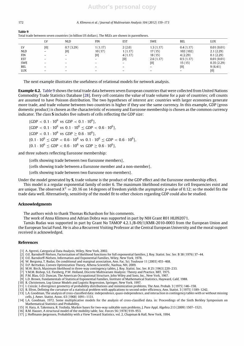
Table 9Total trade between seven countries (in billion US dollars). The MLEs are shown in parentheses.
LV NLD FIN EST SWE BEL LUX
LV [0] 0.7 (3.29) 1 (1.17) 2 (2.0) 1.3 (1.17) 0.4 (1.17) 0.01 (0.01)NLD – [0] 10 (17) 1 (1.17) 17 (15) 102 (102) 2.1 (2.29)FIN – – [0] 4 (1.17) 18 (15) 4 (2.29) 0.1 (2.29)EST – – – [0] 2.6 (1.17) 0.5 (1.17) 0.01 (0.01)SWE – – – – [0] 15 (15) 0.35 (2.29)BEL – – – – – [0] 9 (6.41)LUX – – – – – – [0]
The next example illustrates the usefulness of relational models for network analysis.
Example 6.2. Table 9 shows the total trade data between seven European countries thatwere collected fromUnited NationsCommodity Trade Statistics Database [28]. Every cell contains the value of trade volume for a pair of countries; cell countsare assumed to have Poisson distribution. The two hypotheses of interest are: countries with larger economies generatemore trade, and trade volume between two countries is higher if they use the same currency. In this example, GDP (grossdomestic product) is chosen as the characteristic of economy and Eurozone membership is chosen as the common currencyindicator. The class S includes five subsets of cells reflecting the GDP size:
GDP < 0.1 · 106 vs GDP < 0.1 · 106,
GDP < 0.1 · 106 vs 0.1 · 106≤ GDP < 0.6 · 106
,
GDP < 0.1 · 106 vs GDP ≥ 0.6 · 106,
0.1 · 106≤ GDP < 0.6 · 106 vs 0.1 · 106
≤ GDP < 0.6 · 106,
0.1 · 106≤ GDP < 0.6 · 106 vs GDP ≥ 0.6 · 106
,
and three subsets reflecting Eurozone membership:
cells showing trade between two Eurozone members,cells showing trade between a Eurozone member and a non-member,cells showing trade between two Eurozone non-members.
Under the model generated by S, trade volume is the product of the GDP effect and the Eurozone membership effect.This model is a regular exponential family of order 6. The maximum likelihood estimates for cell frequencies exist and
are unique. The observed X2= 20.16 on 14 degrees of freedom yields the asymptotic p-value of 0.12; so the model fits the
trade data well. Alternatively, sensitivity of the model fit to other choices regarding GDP could also be studied.
Acknowledgments
The authors wish to thank Thomas Richardson for his comments.The work of Anna Klimova and Adrian Dobra was supported in part by NIH Grant R01 HL092071.Tamás Rudas was supported in part by Grant No TAMOP 4.2.1./B-09/1/KMR-2010-0003 from the European Union and
the European Social Fund. He is also a Recurrent Visiting Professor at the Central European University and themoral supportreceived is acknowledged.
References
[1] A. Agresti, Categorical Data Analysis, Wiley, New York, 2002.[2] O.E. Barndorff-Nielsen, Factorization of likelihood functions for full exponential families, J. Roy. Statist. Soc. Ser. B 38 (1976) 37–44.[3] O.E. Barndorff-Nielsen, Information and Exponential Families, Wiley, New York, 1978.[4] W. Bergsma, T. Rudas, On conditional and marginal association, Ann. Fac. Sci. Toulouse 11 (2003) 455–468.[5] D.P. Bertsekas, Convex Optimization Theory, Athena Scientific, Nashua, NH, 2009.[6] M.W. Birch, Maximum likelihood in three-way contingency tables, J. Roy. Statist. Soc. Ser. B 25 (1963) 220–233.[7] Y.M.M. Bishop, S.E. Fienberg, P.W. Holland, Discrete Multivariate Analysis: Theory and Practice, MIT, 1975.[8] P.M. Blau, O.D. Duncan, The American Occupational Structure, John Wiley and Sons, Inc., New York, 1967.[9] L.D. Brown, Fundamentals of Statistical Exponential Families, Institute of Mathematical Statistics, Hayward, Calif, 1988.
[10] R. Christensen, Log-Linear Models and Logistic Regression, Springer, New York, 1997.[11] I. Csiszár, I-divergence geometry of probability distributions and minimization problems, The Ann. Probab. 3 (1975) 146–158.[12] B. Efron, Defining the curvature of a statistical problem with applications to second order efficiency, Ann. Statist. 3 (1975) 1189–1242.[13] L.A. Goodman, The analysis of cross-classified data: independence, quasi-independence, and interaction in contingency tableswith orwithoutmissing
cells, J. Amer. Statist. Assoc. 63 (1968) 1091–1131.[14] L.A. Goodman, 1972. Some multiplicative models for the analysis of cross-classified data. in: Proceedings of the Sixth Berkley Symposium on
Mathematical Statistics and Probability.[15] H. Hara, A. Takemura, R. Yoshida, Markov bases for two-way subtable sum problems, J. Pure Appl. Algebra 213 (2009) 1507–1521.[16] R.M. Hauser, A structural model of the mobility table, Soc. Forces 56 (1978) 919–953.[17] J. Hoffmann-Jørgensen, Probability with a View Toward Statistics, vol. 2, Chapman & Hall, New York, 1994.

Author's personal copy
A. Klimova et al. / Journal of Multivariate Analysis 104 (2012) 159–173 173
[18] M. Hout, Mobility Tables, vol. 31, Sage Publications, Inc., 1983.[19] R.E. Kass, P.W. Vos, Geometrical Foundations of Asymptotic Inference, Wiley, New York, 1997.[20] G. Kawamura, T.Matsuoka, T. Tajiri,M.Nishida,M.Hayashi, Effectiveness of a sugarcane-fish combination as bait in trapping swimming crabs, Fisheries
Research 22 (1995) 155–160.[21] L. Pachter, B. Sturmfels (Eds.), Algebraic Statistic for Computational Biology, Cambridge University Press, 2005.[22] T. Rudas, Odds Ratios in the Analysis of Contingency Tables, Sage Publications, Inc., 1998.[23] W. Rudin, Principles of Mathematical Analysis, McGraw-Hill, 1976.[24] A. Schrijver, Theory of Linear and Integer Programming, Wiley, New York, 1986.[25] B. Sturmfels, Gröbner Bases and Convex Polytopes, AMS, Providence RI, 1996.[26] M.A. Tanner, M.A. Young, Modeling agreement among raters, J. Amer. Statist. Assoc. 80 (1985) 175–180.[27] M.A. Tanner, M.A. Young, Modeling agreement among raters, Psychol. Bull. 98 (1985) 408–415.[28] United nations commodity trade statistics database. 2007 Available from http://comtrade.un.org/.[29] D. Zelterman, T.I. Youn, Indicator models for social mobility tables, Comput. Statist. Data Anal. 14 (1992).
Related Documents