NCSS Statistical Software NCSS.com 501-1 © NCSS, LLC. All Rights Reserved. Chapter 501 Contingency Tables (Crosstabs / Chi- Square Test) Introduction This procedure produces tables of counts and percentages for the joint distribution of two categorical variables. Such tables are known as contingency, cross-tabulation, or crosstab tables. When a breakdown of more than two variables is desired, you can specify up to eight grouping (break) variables in addition to the two table variables. A separate table is generated for each unique set of values of these grouping variables. The data can also be entered directly as a two-way table for analysis. This procedure serves as a summary reporting tool and is often used to analyze survey data. It calculates most of the popular contingency-table statistics and tests such as chi-square, Fisher’s exact, and McNemar’s tests, as well as the Cochran-Armitage test for trend in proportions and the Kappa and weighted Kappa tests for inter-rater agreement. This procedure also produces a broad set of association and correlation statistics for contingency tables: Phi, Cramer’s V, Pearson’s Contingency Coefficient, Tschuprow’s T, Lamba, Kendall’s Tau, and Gamma. Types of Categorical Variables Note that we will refer to two types of categorical variables: Table variables and Grouping variables. The values of the Table variables are used to define the rows and columns of a single contingency table. Two Table variables are used for each table, one variable defining the rows of the table and the other defining the columns. Grouping variables are used to split a data into subgroups. A separate table is generated for each unique set of values of the Grouping variables. Note that if you only want to use one Table variable, you should use the Frequency Table procedure.

Welcome message from author
This document is posted to help you gain knowledge. Please leave a comment to let me know what you think about it! Share it to your friends and learn new things together.
Transcript

NCSS Statistical Software NCSS.com
501-1 © NCSS, LLC. All Rights Reserved.
Chapter 501
Contingency Tables (Crosstabs / Chi-Square Test) Introduction This procedure produces tables of counts and percentages for the joint distribution of two categorical variables. Such tables are known as contingency, cross-tabulation, or crosstab tables. When a breakdown of more than two variables is desired, you can specify up to eight grouping (break) variables in addition to the two table variables. A separate table is generated for each unique set of values of these grouping variables. The data can also be entered directly as a two-way table for analysis.
This procedure serves as a summary reporting tool and is often used to analyze survey data. It calculates most of the popular contingency-table statistics and tests such as chi-square, Fisher’s exact, and McNemar’s tests, as well as the Cochran-Armitage test for trend in proportions and the Kappa and weighted Kappa tests for inter-rater agreement.
This procedure also produces a broad set of association and correlation statistics for contingency tables: Phi, Cramer’s V, Pearson’s Contingency Coefficient, Tschuprow’s T, Lamba, Kendall’s Tau, and Gamma.
Types of Categorical Variables Note that we will refer to two types of categorical variables: Table variables and Grouping variables. The values of the Table variables are used to define the rows and columns of a single contingency table. Two Table variables are used for each table, one variable defining the rows of the table and the other defining the columns. Grouping variables are used to split a data into subgroups. A separate table is generated for each unique set of values of the Grouping variables.
Note that if you only want to use one Table variable, you should use the Frequency Table procedure.

NCSS Statistical Software NCSS.com Contingency Tables (Crosstabs / Chi-Square Test)
501-2 © NCSS, LLC. All Rights Reserved.
Technical Details For the technical details that follow, we assume a contingency table of counts with R rows and C columns as in the table below. Let 𝑂𝑂𝑖𝑖𝑖𝑖 be the observed count for the ith row (i = 1 to R) and jth column (j = 1 to C). Let the row
Column Variable Column 1 ⋯ Column j ⋯ Column C Total
Row Variable Row 1 𝑂𝑂11 ⋯ 𝑂𝑂1𝑖𝑖 ⋯ 𝑂𝑂1𝐶𝐶 𝑛𝑛1∙ ⋮ ⋮ ⋱ ⋮ ⋰ ⋮ ⋮ Row i 𝑂𝑂𝑖𝑖1 ⋯ 𝑂𝑂𝑖𝑖𝑖𝑖 ⋯ 𝑂𝑂𝑖𝑖𝐶𝐶 𝑛𝑛𝑖𝑖∙ ⋮ ⋮ ⋰ ⋮ ⋱ ⋮ ⋮ Row R 𝑂𝑂𝑅𝑅1 ⋯ 𝑂𝑂𝑅𝑅𝑖𝑖 ⋯ 𝑂𝑂𝑅𝑅𝐶𝐶 𝑛𝑛𝑅𝑅∙
Total 𝑛𝑛∙1 ⋯ 𝑛𝑛∙𝑖𝑖 ⋯ 𝑛𝑛∙𝐶𝐶 1
and column marginal totals be designated as 𝑛𝑛𝑖𝑖∙ and 𝑛𝑛∙𝑖𝑖, respectively, where
𝑛𝑛𝑖𝑖∙ = �𝑂𝑂𝑖𝑖𝑖𝑖𝑖𝑖
𝑛𝑛∙𝑖𝑖 = �𝑂𝑂𝑖𝑖𝑖𝑖𝑖𝑖
Let the total number of counts in the table be N, where
𝑁𝑁 = ��𝑂𝑂𝑖𝑖𝑖𝑖𝑖𝑖𝑖𝑖
= �𝑛𝑛𝑖𝑖∙𝑖𝑖
= �𝑛𝑛∙𝑖𝑖𝑖𝑖
The table of associated proportions can then be written as
Column Variable Column 1 ⋯ Column j ⋯ Column C Total
Row Variable Row 1 𝑝𝑝11 ⋯ 𝑝𝑝1𝑖𝑖 ⋯ 𝑝𝑝1𝐶𝐶 𝑝𝑝1∙ ⋮ ⋮ ⋱ ⋮ ⋰ ⋮ ⋮ Row i 𝑝𝑝𝑖𝑖1 ⋯ 𝑝𝑝𝑖𝑖𝑖𝑖 ⋯ 𝑝𝑝𝑖𝑖𝐶𝐶 𝑝𝑝𝑖𝑖∙ ⋮ ⋮ ⋰ ⋮ ⋱ ⋮ ⋮ Row R 𝑝𝑝𝑅𝑅1 ⋯ 𝑝𝑝𝑅𝑅𝑖𝑖 ⋯ 𝑝𝑝𝑅𝑅𝐶𝐶 𝑝𝑝𝑅𝑅∙
Total 𝑝𝑝∙1 ⋯ 𝑝𝑝∙𝑖𝑖 ⋯ 𝑝𝑝∙𝐶𝐶 1

NCSS Statistical Software NCSS.com Contingency Tables (Crosstabs / Chi-Square Test)
501-3 © NCSS, LLC. All Rights Reserved.
where
𝑝𝑝𝑖𝑖𝑖𝑖 =𝑂𝑂𝑖𝑖𝑖𝑖𝑁𝑁
𝑝𝑝𝑖𝑖∙ =𝑛𝑛𝑖𝑖∙𝑁𝑁
𝑝𝑝∙𝑖𝑖 =𝑛𝑛∙𝑖𝑖𝑁𝑁
Finally, designate the expected counts and expected proportions for the ith row and jth column as 𝐸𝐸𝑖𝑖𝑖𝑖 and 𝑃𝑃𝑃𝑃𝑖𝑖𝑖𝑖, respectively, where
𝐸𝐸𝑖𝑖𝑖𝑖 =𝑛𝑛𝑖𝑖∙𝑛𝑛∙𝑖𝑖𝑁𝑁
𝑃𝑃𝑒𝑒𝑖𝑖𝑖𝑖 =𝐸𝐸𝑖𝑖𝑖𝑖𝑁𝑁
= 𝑝𝑝𝑖𝑖∙𝑝𝑝∙𝑖𝑖
In the sections that follow we will describe the various tests and statistics calculated by this procedure using the preceding notation.
Table Statistics This section presents various statistics that can be output for each individual cell. These are useful for studying the independence between rows and columns. The statistics for the ith row and jth column are as follows.
Count The cell count, 𝑂𝑂𝑖𝑖𝑖𝑖, is the number of observations for the cell.
Row Percentage The percentage for column j within row i, 𝑝𝑝𝑖𝑖|𝑖𝑖, is calculated as
𝑝𝑝𝑖𝑖|𝑖𝑖 =𝑂𝑂𝑖𝑖𝑖𝑖𝑛𝑛𝑖𝑖∙
Column Percentage The percentage for row i within column j, 𝑝𝑝𝑖𝑖|𝑖𝑖, is calculated as
𝑝𝑝𝑖𝑖|𝑖𝑖 =𝑂𝑂𝑖𝑖𝑖𝑖𝑛𝑛∙𝑖𝑖
Table Percentage The overall percentage for the cell, 𝑝𝑝𝑖𝑖𝑖𝑖, is calculated as
𝑝𝑝𝑖𝑖𝑖𝑖 =𝑂𝑂𝑖𝑖𝑖𝑖𝑁𝑁
Expected Counts Assuming Independence The expected count, 𝐸𝐸𝑖𝑖𝑖𝑖, is the count that would be obtained if the hypothesis of row-column independence were true. It is calculated as
𝐸𝐸𝑖𝑖𝑖𝑖 =𝑛𝑛𝑖𝑖∙𝑛𝑛∙𝑖𝑖𝑁𝑁

NCSS Statistical Software NCSS.com Contingency Tables (Crosstabs / Chi-Square Test)
501-4 © NCSS, LLC. All Rights Reserved.
Chi-Square Contribution The chi-square contribution, 𝐶𝐶𝐶𝐶𝑖𝑖𝑖𝑖, measures the amount that a cell contributes to the overall chi-square statistic for the table. This and the next two items let you determine which cells impact the chi-square statistic the most.
𝐶𝐶𝐶𝐶𝑖𝑖𝑖𝑖 =�𝑂𝑂𝑖𝑖𝑖𝑖 − 𝐸𝐸𝑖𝑖𝑖𝑖�
2
𝐸𝐸𝑖𝑖𝑖𝑖
Deviation from Independence The deviation statistic, 𝐷𝐷𝑖𝑖𝑖𝑖, measures how much the observed count differs from the expected count.
𝐷𝐷𝑖𝑖𝑖𝑖 = 𝑂𝑂𝑖𝑖𝑖𝑖 − 𝐸𝐸𝑖𝑖𝑖𝑖
Std. Residual The standardized residual, 𝐶𝐶𝑆𝑆𝑖𝑖𝑖𝑖, is equal to the deviation divided by the square root of the expected value:
𝐶𝐶𝑆𝑆𝑖𝑖𝑖𝑖 =𝑂𝑂𝑖𝑖𝑖𝑖 − 𝐸𝐸𝑖𝑖𝑖𝑖�𝐸𝐸𝑖𝑖𝑖𝑖
Tests for Row-Column Independence
Pearson’s Chi-Square Test Pearson’s chi-square statistic is used to test independence between the row and column variables. Independence means that knowing the value of the row variable does not change the probabilities of the column variable (and vice versa). Another way of looking at independence is to say that the row percentages (or column percentages) remain constant from row to row (or column to column).
This test requires large sample sizes to be accurate. An often quoted rule of thumb regarding sample size is that none of the expected cell values should be less than five. Although some users ignore the sample size requirement, you should also be very skeptical of the test if you have cells in your table with zero counts. For 2 × 2 tables, consider using Yates’ Continuity Correction or Fisher’s Exact Test for small samples.
Pearson’s chi-square test statistic follows an asymptotic chi-square distribution with (R – 1)(C – 1) degrees of freedom when the row and column variables are independent. It is calculated as
𝜒𝜒𝑃𝑃2 = ���𝑂𝑂𝑖𝑖𝑖𝑖 − 𝐸𝐸𝑖𝑖𝑖𝑖�
2
𝐸𝐸𝑖𝑖𝑖𝑖𝑖𝑖𝑖𝑖
.
Yates’ Continuity Corrected Chi-Square Test (2 × 2 Tables) Yates’ Continuity Corrected Chi-Square Test (or just Yates’ Continuity Correction) is similar to Pearson's chi-square test, but is adjusted for the continuity of the chi-square distribution. This test is particularly useful when you have small sample sizes. This test is only calculated for 2 × 2 tables.
Yates’ continuity corrected test statistic follows an asymptotic chi-square distribution with (R – 1)(C – 1) degrees of freedom when the row and column variables are independent. It is calculated as
𝜒𝜒𝑌𝑌2 = ���𝑚𝑚𝑚𝑚𝑚𝑚�0, �𝑂𝑂𝑖𝑖𝑖𝑖 − 𝐸𝐸𝑖𝑖𝑖𝑖� − 0.5��
2
𝐸𝐸𝑖𝑖𝑖𝑖.
𝑖𝑖𝑖𝑖

NCSS Statistical Software NCSS.com Contingency Tables (Crosstabs / Chi-Square Test)
501-5 © NCSS, LLC. All Rights Reserved.
Likelihood Ratio Test This test makes use of the fact that under the null hypothesis of independence, the likelihood ratio statistic follows an asymptotic chi-square distribution.
The likelihood ratio test statistic follows an asymptotic chi-square distribution with (R – 1)(C – 1) degrees of freedom when the row and column variables are independent. It is calculated as
𝜒𝜒𝐿𝐿𝑅𝑅2 = 2��𝑂𝑂𝑖𝑖𝑖𝑖ln�𝑂𝑂𝑖𝑖𝑖𝑖𝐸𝐸𝑖𝑖𝑖𝑖
� .𝑖𝑖𝑖𝑖
Fisher’s Exact Test (2 × 2 Tables) This test was designed to test the hypothesis that the two column percentages in a 2 × 2 table are equal. It is especially useful when sample sizes are small (even zero in some cells) and the chi-square test is not appropriate.
Using the hypergeometric distribution with fixed row and column totals, this test computes probabilities of all possible tables with the observed row and column totals. This test is often used when sample sizes are small, but it is appropriate for all sample sizes because Fisher’s exact test does not depend on any large-sample asymptotic distribution assumptions. This test is only calculated for 2 × 2 tables.
If we assume that 𝑃𝑃𝐻𝐻is the hypergeometric probability of any table with the observed row and column marginal totals, then Fisher’s Exact Test probabilities are calculated by summing over defined sets of tables depending on the hypothesis being tested (one-sided or two-sided).
Define the difference between conditional column proportions for row 1 from the observed table as 𝐷𝐷𝑂𝑂, with
𝐷𝐷𝑂𝑂 = 𝑝𝑝1|1 − 𝑝𝑝1|2
and the difference between conditional column proportions for row 1 from other possible tables with the observed row and column marginal totals as 𝐷𝐷, with
𝐷𝐷 = 𝑝𝑝1|1 − 𝑝𝑝1|2
The two-sided Fisher’s Exact Test P-value is calculated as
𝑃𝑃 − 𝑉𝑉𝑚𝑚𝑉𝑉𝑉𝑉𝑃𝑃𝑇𝑇𝑇𝑇𝑇𝑇−𝑆𝑆𝑖𝑖𝑆𝑆𝑒𝑒𝑆𝑆 = � 𝑃𝑃𝐻𝐻𝑇𝑇𝑇𝑇𝑇𝑇𝑇𝑇𝑒𝑒𝑇𝑇 𝑇𝑇ℎ𝑒𝑒𝑒𝑒𝑒𝑒 |𝐷𝐷|≥|𝐷𝐷𝑂𝑂|
The lower one-sided Fisher’s Exact Test P-value is calculated as
𝑃𝑃 − 𝑉𝑉𝑚𝑚𝑉𝑉𝑉𝑉𝑃𝑃𝐿𝐿𝑇𝑇𝑇𝑇𝑒𝑒𝑒𝑒 = � 𝑃𝑃𝐻𝐻𝑇𝑇𝑇𝑇𝑇𝑇𝑇𝑇𝑒𝑒𝑇𝑇 𝑇𝑇ℎ𝑒𝑒𝑒𝑒𝑒𝑒 𝐷𝐷≤𝐷𝐷𝑂𝑂
The upper one-sided Fisher’s Exact Test P-value is calculated as
𝑃𝑃 − 𝑉𝑉𝑚𝑚𝑉𝑉𝑉𝑉𝑃𝑃𝑈𝑈𝑈𝑈𝑈𝑈𝑒𝑒𝑒𝑒 = � 𝑃𝑃𝐻𝐻𝑇𝑇𝑇𝑇𝑇𝑇𝑇𝑇𝑒𝑒𝑇𝑇 𝑇𝑇ℎ𝑒𝑒𝑒𝑒𝑒𝑒 𝐷𝐷≥𝐷𝐷𝑂𝑂

NCSS Statistical Software NCSS.com Contingency Tables (Crosstabs / Chi-Square Test)
501-6 © NCSS, LLC. All Rights Reserved.
Tests for Trend in Proportions (2 × k Tables) When one variable is ordinal (e.g. “Low, Medium, High” or “1, 2, 3, 4, 5”) and the other has exactly two levels (e.g. “success”, “failure”), you can test the hypothesis that there is a linear trend in the proportion of successes (i.e. that the true proportion of successes increases (or decreases) across the levels of the ordinal variable). Three tests for linear trend in proportions are available in NCSS: the Cochran-Armitage Test, the Cochran-Armitage Test with Continuity Correction, and the Armitage Rank Correlation Test. Of these, the Cochran-Armitage Test is the most widely used.
Cochran-Armitage Test The Cochran-Armitage test is described in Cochran (1954) and Armitage (1955). Though the formulas that follow appear different from those presented in the articles, the results are equivalent.
Suppose we have k independent binomial variates, iy , with response probabilities, ip , based on samples of size
in at covariate (or dose) levels, ix , for i = 1, 2, …, k, where kxxx <<< ...21 . The scores ix , come from the row (or column) names of the ordinal variable. When the names are numeric (e.g. “1 2 3 4 etc.”) then the actual numeric values are used for the scores, allowing the user to input unequally spaced score values. When the names are not numeric, even though they may represent an ordinal scale (e.g. “Low, Medium, High”), then the scores are assigned automatically as evenly spaced integers from 1 to k.
Define the following:
∑=
=k
iinN
1
∑=
=k
iiy
Np
1
1
pq −=1
∑=
=k
iii xn
Nx
1
1
If we assume that the probability of response follows a linear trend on the logistic scale, then
( )( )i
ii x
xpβα
βα++
+=
exp1exp .
The Cochran-Armitage test can be used to test the following hypotheses:
One-Sided (Increasing Trend) kpppH === ...: 210 vs. kpppH <<< ...: 211
One-Sided (Decreasing Trend) kpppH === ...: 210 vs. kpppH >>> ...: 211
Two-Sided kpppH === ...: 210 vs. kpppH <<< ...: 211 or kppp >>> ...21
Nam (1987) presents the following asymptotic test statistic for detecting a linear trend in proportions
( )
( )
−
−=
∑
∑
=
=
k
iii
k
iii
xxnqp
xxyz
1
2
1 .

NCSS Statistical Software NCSS.com Contingency Tables (Crosstabs / Chi-Square Test)
501-7 © NCSS, LLC. All Rights Reserved.
A one-sided test rejects H0 in favor of an increasing trend if α−≥ 1zz , where α−1z is the value that leaves 1 – α in the upper tail of the standard normal distribution. A one-sided test rejects H0 in favor of a decreasing trend if
αzz ≤ , where αz is the value that leaves α in the lower tail of the standard normal distribution. A two-sided test rejects H0 in favor of either an increasing or decreasing trend if 2/1 α−≥ zz .
Cochran-Armitage Test with Continuity Correction The Cochran-Armitage test with continuity correction is nearly the same as the uncorrected Cochran-Armitage test described earlier. In the continuity corrected test, a small continuity correction factor, 2/∆ , is added or subtracted from the numerator, depending on the direction of the test. If the scores, ix , are equally-spaced then
ii xx −=∆ +1 for all i < k
or the interval between adjacent scores. NCSS computes ∆ for unequally-spaced scores as
( )∑−
=+ −
−=∆
1
111
1 k
iii xx
k.
For the case of unequally-spaced covariates, Nam (1987) states, “For unequally spaced doses, no constant correction is adequate for all outcomes.” Therefore, we caution against the use of the continuity-corrected test statistic in the case of unequally-spaced covariates.
Using the same notation as that described for the Cochran-Armitage test, Nam (1987) presents the following continuity corrected asymptotic test statistic for detecting an increasing linear trend in proportions
( )
( )
−
∆−−
=
∑
∑
=
=
k
iii
k
iii
Ucc
xxnqp
xxyz
1
2
1..
2.
A one-sided test rejects H0 in favor of an increasing trend if α−≥ 1.. zz Ucc , where α−1z is the value that leaves 1 – α in the upper tail of the standard normal distribution.
The continuity-corrected test statistic for a decreasing trend is the same as that for an increasing trend, except that 2/∆ is added in the numerator instead of subtracted
( )
( )
−
∆+−
=
∑
∑
=
=
k
iii
k
iii
Lcc
xxnqp
xxyz
1
2
1..
2.
A one-sided test rejects H0 in favor of a decreasing trend if αzz Lcc ≤.. , where αz is the value that leaves α in the lower tail of the standard normal distribution.
A two-sided test rejects H0 in favor of either an increasing or decreasing trend if 2/1.. α−≥ zz Ucc or if 2/.. αzz Lcc ≤ .
NCSS Statistical Software NCSS.com Contingency Tables (Crosstabs / Chi-Square Test)
501-8 © NCSS, LLC. All Rights Reserved.
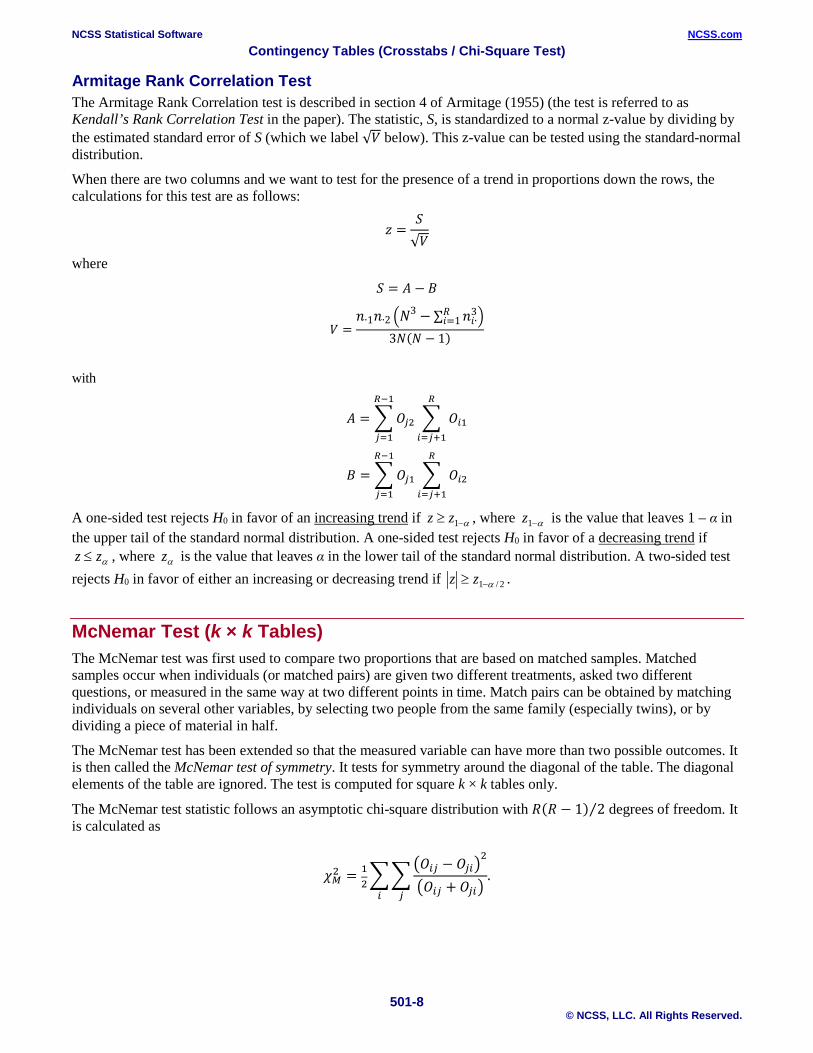
Armitage Rank Correlation Test The Armitage Rank Correlation test is described in section 4 of Armitage (1955) (the test is referred to as Kendall’s Rank Correlation Test in the paper). The statistic, S, is standardized to a normal z-value by dividing by the estimated standard error of S (which we label √𝑉𝑉 below). This z-value can be tested using the standard-normal distribution.
When there are two columns and we want to test for the presence of a trend in proportions down the rows, the calculations for this test are as follows:
𝑧𝑧 =𝐶𝐶√𝑉𝑉
where
𝐶𝐶 = 𝐴𝐴 − 𝐵𝐵
𝑉𝑉 =𝑛𝑛∙1𝑛𝑛∙2 �𝑁𝑁3 −∑ 𝑛𝑛𝑖𝑖∙3𝑆𝑆
𝑖𝑖=1 �3𝑁𝑁(𝑁𝑁 − 1)
with
𝐴𝐴 = �𝑂𝑂𝑖𝑖2 � 𝑂𝑂𝑖𝑖1
𝑅𝑅
𝑖𝑖=𝑖𝑖+1
𝑅𝑅−1
𝑖𝑖=1
𝐵𝐵 = �𝑂𝑂𝑖𝑖1 � 𝑂𝑂𝑖𝑖2
𝑅𝑅
𝑖𝑖=𝑖𝑖+1
𝑅𝑅−1
𝑖𝑖=1
A one-sided test rejects H0 in favor of an increasing trend if α−≥ 1zz , where α−1z is the value that leaves 1 – α in the upper tail of the standard normal distribution. A one-sided test rejects H0 in favor of a decreasing trend if
αzz ≤ , where αz is the value that leaves α in the lower tail of the standard normal distribution. A two-sided test rejects H0 in favor of either an increasing or decreasing trend if 2/1 α−≥ zz .
McNemar Test (k × k Tables) The McNemar test was first used to compare two proportions that are based on matched samples. Matched samples occur when individuals (or matched pairs) are given two different treatments, asked two different questions, or measured in the same way at two different points in time. Match pairs can be obtained by matching individuals on several other variables, by selecting two people from the same family (especially twins), or by dividing a piece of material in half.
The McNemar test has been extended so that the measured variable can have more than two possible outcomes. It is then called the McNemar test of symmetry. It tests for symmetry around the diagonal of the table. The diagonal elements of the table are ignored. The test is computed for square k × k tables only.
The McNemar test statistic follows an asymptotic chi-square distribution with 𝑆𝑆(𝑆𝑆 − 1) 2⁄ degrees of freedom. It is calculated as
𝜒𝜒𝑀𝑀2 = 12��
�𝑂𝑂𝑖𝑖𝑖𝑖 − 𝑂𝑂𝑖𝑖𝑖𝑖�2
�𝑂𝑂𝑖𝑖𝑖𝑖 + 𝑂𝑂𝑖𝑖𝑖𝑖�𝑖𝑖𝑖𝑖
.

NCSS Statistical Software NCSS.com Contingency Tables (Crosstabs / Chi-Square Test)
501-9 © NCSS, LLC. All Rights Reserved.
Kappa and Weighted Kappa Tests for Inter-Rater Agreement (k × k Tables) Kappa is a measure of association (correlation or reliability) between two measurements on the same individual when the measurements are categorical. It tests if the counts along the diagonal are significantly large. Because Kappa is used when the same variable is measured twice, it is only appropriate for square tables where the row and column categories are the same. Kappa is often used to study the agreement of two raters such as judges or doctors, where each rater classifies each individual into one of k categories.
Rules-of-thumb for kappa: values less than 0.40 indicate low association; values between 0.40 and 0.75 indicate medium association; and values greater than 0.75 indicate high association between the two raters.
Kappa and weighted kappa are only output for square k × k tables with identical row and column labels. If your data have entire rows or columns missing because they were never reported by the raters, you must add a row or column of zeros to make the table square (see Example 6).
The results of this section are based on Fleiss, Levin, and Paik (2003). The kappa procedure also outputs the Maximum Kappa and Maximum-Adjusted Kappa statistics.
Kappa Estimation Define the overall proportion of observed agreement, 𝑝𝑝𝑇𝑇, as
𝑝𝑝𝑇𝑇 = �𝑝𝑝𝑖𝑖𝑖𝑖𝑖𝑖
and the overall chance-expected proportion of agreement, 𝑝𝑝𝑒𝑒, as
𝑝𝑝𝑒𝑒 = �𝑝𝑝𝑖𝑖∙𝑝𝑝∙𝑖𝑖𝑖𝑖
Kappa is calculated as from 𝑝𝑝𝑇𝑇 and 𝑝𝑝𝑒𝑒 as
�̂�𝜅 =𝑝𝑝𝑇𝑇 − 𝑝𝑝𝑒𝑒1 − 𝑝𝑝𝑒𝑒
with asymptotic standard error
𝐶𝐶𝐸𝐸�𝜅𝜅� =√𝐴𝐴 + 𝐵𝐵 − 𝐶𝐶(1 − 𝑝𝑝𝑒𝑒)√𝑁𝑁
where
𝐴𝐴 = �𝑝𝑝𝑖𝑖𝑖𝑖[1 − (𝑝𝑝𝑖𝑖∙ + 𝑝𝑝∙𝑖𝑖)(1 − �̂�𝜅)]2𝑖𝑖
𝐵𝐵 = (1 − �̂�𝜅)2��𝑝𝑝𝑖𝑖𝑖𝑖�𝑝𝑝∙𝑖𝑖 + 𝑝𝑝𝑖𝑖∙�2
𝑖𝑖≠𝑖𝑖𝑖𝑖
𝐶𝐶 = [�̂�𝜅 − 𝑝𝑝𝑒𝑒(1 − �̂�𝜅)]2
An approximate 100(1− 𝛼𝛼)% confidence interval for 𝜅𝜅 is
�̂�𝜅 − 𝑧𝑧𝛼𝛼 2⁄ 𝐶𝐶𝐸𝐸�𝜅𝜅� ≤ 𝜅𝜅 ≤ �̂�𝜅 + 𝑧𝑧𝛼𝛼 2⁄ 𝐶𝐶𝐸𝐸�𝜅𝜅�
NCSS Statistical Software NCSS.com Contingency Tables (Crosstabs / Chi-Square Test)
501-10 © NCSS, LLC. All Rights Reserved.
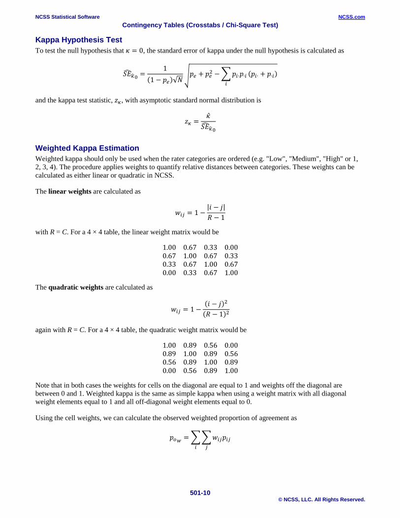
Kappa Hypothesis Test To test the null hypothesis that 𝜅𝜅 = 0, the standard error of kappa under the null hypothesis is calculated as
𝐶𝐶𝐸𝐸�𝜅𝜅�0 =1
(1 − 𝑝𝑝𝑒𝑒)√𝑁𝑁�𝑝𝑝𝑒𝑒 + 𝑝𝑝𝑒𝑒2 −�𝑝𝑝𝑖𝑖∙𝑝𝑝∙𝑖𝑖
𝑖𝑖
(𝑝𝑝𝑖𝑖∙ + 𝑝𝑝∙𝑖𝑖)
and the kappa test statistic, 𝑧𝑧𝜅𝜅, with asymptotic standard normal distribution is
𝑧𝑧𝜅𝜅 =�̂�𝜅
𝐶𝐶𝐸𝐸�𝜅𝜅�0
Weighted Kappa Estimation Weighted kappa should only be used when the rater categories are ordered (e.g. "Low", "Medium", "High" or 1, 2, 3, 4). The procedure applies weights to quantify relative distances between categories. These weights can be calculated as either linear or quadratic in NCSS.
The linear weights are calculated as
𝑤𝑤𝑖𝑖𝑖𝑖 = 1 −|𝑖𝑖 − 𝑗𝑗|𝑆𝑆 − 1
with R = C. For a 4 × 4 table, the linear weight matrix would be
1.00 0.67 0.33 0.000.67 1.00 0.67 0.330.33 0.67 1.00 0.670.00 0.33 0.67 1.00
The quadratic weights are calculated as
𝑤𝑤𝑖𝑖𝑖𝑖 = 1 −(𝑖𝑖 − 𝑗𝑗)2
(𝑆𝑆 − 1)2
again with R = C. For a 4 × 4 table, the quadratic weight matrix would be
1.00 0.89 0.56 0.000.89 1.00 0.89 0.560.56 0.89 1.00 0.890.00 0.56 0.89 1.00
Note that in both cases the weights for cells on the diagonal are equal to 1 and weights off the diagonal are between 0 and 1. Weighted kappa is the same as simple kappa when using a weight matrix with all diagonal weight elements equal to 1 and all off-diagonal weight elements equal to 0.
Using the cell weights, we can calculate the observed weighted proportion of agreement as
𝑝𝑝𝑇𝑇𝑇𝑇 = ��𝑤𝑤𝑖𝑖𝑖𝑖𝑝𝑝𝑖𝑖𝑖𝑖𝑖𝑖𝑖𝑖

NCSS Statistical Software NCSS.com Contingency Tables (Crosstabs / Chi-Square Test)
501-11 © NCSS, LLC. All Rights Reserved.
and the overall chance-expected weighted proportion of agreement, 𝑝𝑝𝑒𝑒, as
𝑝𝑝𝑒𝑒𝑇𝑇 = ��𝑤𝑤𝑖𝑖𝑖𝑖𝑝𝑝𝑖𝑖∙𝑝𝑝∙𝑖𝑖𝑖𝑖𝑖𝑖
Further define
𝑤𝑤�𝑖𝑖∙ = �𝑤𝑤𝑖𝑖𝑖𝑖𝑝𝑝∙𝑖𝑖𝑖𝑖
𝑤𝑤�∙𝑖𝑖 = �𝑤𝑤𝑖𝑖𝑖𝑖𝑝𝑝𝑖𝑖∙𝑖𝑖
Weighted kappa is calculated as
�̂�𝜅𝑇𝑇 =𝑝𝑝𝑇𝑇𝑇𝑇 − 𝑝𝑝𝑒𝑒𝑇𝑇
1 − 𝑝𝑝𝑒𝑒𝑇𝑇
with asymptotic standard error
𝐶𝐶𝐸𝐸�𝜅𝜅�𝑤𝑤 =√𝐴𝐴 − 𝐵𝐵
�1 − 𝑝𝑝𝑒𝑒𝑇𝑇�√𝑁𝑁
where
𝐴𝐴 = ��𝑝𝑝𝑖𝑖𝑖𝑖�𝑤𝑤𝑖𝑖𝑖𝑖 − �𝑤𝑤�𝑖𝑖∙ + 𝑤𝑤�∙𝑖𝑖�(1 − �̂�𝜅𝑇𝑇)�2
𝑖𝑖𝑖𝑖
𝐵𝐵 = ��̂�𝜅𝑇𝑇 − 𝑝𝑝𝑒𝑒𝑇𝑇(1− �̂�𝜅𝑇𝑇)�2
An approximate 100(1− 𝛼𝛼)% confidence interval for 𝜅𝜅𝑇𝑇 is
�̂�𝜅𝑇𝑇 − 𝑧𝑧𝛼𝛼 2⁄ 𝐶𝐶𝐸𝐸�𝜅𝜅�𝑤𝑤 ≤ 𝜅𝜅𝑇𝑇 ≤ �̂�𝜅𝑇𝑇 + 𝑧𝑧𝛼𝛼 2⁄ 𝐶𝐶𝐸𝐸�𝜅𝜅�𝑤𝑤
Weighted Kappa Hypothesis Test To test the null hypothesis that 𝜅𝜅𝑇𝑇 = 0, the standard error of weighted kappa under the null hypothesis is calculated as
𝐶𝐶𝐸𝐸�𝜅𝜅�𝑇𝑇0=
1�1 − 𝑝𝑝𝑒𝑒𝑇𝑇�√𝑁𝑁
���𝑝𝑝𝑖𝑖∙𝑝𝑝∙𝑖𝑖�𝑤𝑤𝑖𝑖𝑖𝑖 − �𝑤𝑤�𝑖𝑖∙ + 𝑤𝑤�∙𝑖𝑖��2
𝑖𝑖𝑖𝑖
− 𝑝𝑝𝑒𝑒𝑤𝑤2
and the weighted kappa test statistic, 𝑧𝑧𝜅𝜅𝑤𝑤, with asymptotic standard normal distribution is
𝑧𝑧𝜅𝜅𝑤𝑤 =�̂�𝜅𝑇𝑇
𝐶𝐶𝐸𝐸�𝜅𝜅�𝑇𝑇0
NCSS Statistical Software NCSS.com Contingency Tables (Crosstabs / Chi-Square Test)
501-12 © NCSS, LLC. All Rights Reserved.
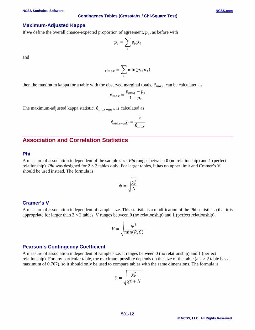
Maximum-Adjusted Kappa If we define the overall chance-expected proportion of agreement, 𝑝𝑝𝑒𝑒, as before with
𝑝𝑝𝑒𝑒 = �𝑝𝑝𝑖𝑖∙𝑝𝑝∙𝑖𝑖𝑖𝑖
and
𝑝𝑝𝑚𝑚𝑇𝑇𝑚𝑚 = �min(𝑝𝑝𝑖𝑖∙,𝑝𝑝∙𝑖𝑖)𝑖𝑖
then the maximum kappa for a table with the observed marginal totals, �̂�𝜅𝑚𝑚𝑇𝑇𝑚𝑚, can be calculated as
�̂�𝜅𝑚𝑚𝑇𝑇𝑚𝑚 =𝑝𝑝𝑚𝑚𝑇𝑇𝑚𝑚 − 𝑝𝑝𝑒𝑒
1 − 𝑝𝑝𝑒𝑒
The maximum-adjusted kappa statistic, �̂�𝜅𝑚𝑚𝑇𝑇𝑚𝑚−𝑇𝑇𝑆𝑆𝑖𝑖, is calculated as
�̂�𝜅𝑚𝑚𝑇𝑇𝑚𝑚−𝑇𝑇𝑆𝑆𝑖𝑖 =�̂�𝜅
�̂�𝜅𝑚𝑚𝑇𝑇𝑚𝑚
Association and Correlation Statistics
Phi A measure of association independent of the sample size. Phi ranges between 0 (no relationship) and 1 (perfect relationship). Phi was designed for 2 × 2 tables only. For larger tables, it has no upper limit and Cramer’s V should be used instead. The formula is
𝜙𝜙 = �𝜒𝜒𝑃𝑃2
𝑁𝑁
Cramer’s V A measure of association independent of sample size. This statistic is a modification of the Phi statistic so that it is appropriate for larger than 2 × 2 tables. V ranges between 0 (no relationship) and 1 (perfect relationship).
𝑉𝑉 = �𝜙𝜙2
min(𝑆𝑆,𝐶𝐶)
Pearson’s Contingency Coefficient A measure of association independent of sample size. It ranges between 0 (no relationship) and 1 (perfect relationship). For any particular table, the maximum possible depends on the size of the table (a 2 × 2 table has a maximum of 0.707), so it should only be used to compare tables with the same dimensions. The formula is
𝐶𝐶 = �𝜒𝜒𝑃𝑃2
𝜒𝜒𝑃𝑃2 + 𝑁𝑁
NCSS Statistical Software NCSS.com Contingency Tables (Crosstabs / Chi-Square Test)
501-13 © NCSS, LLC. All Rights Reserved.
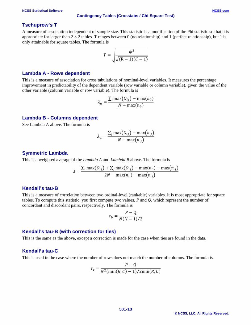
Tschuprow’s T A measure of association independent of sample size. This statistic is a modification of the Phi statistic so that it is appropriate for larger than 2 × 2 tables. T ranges between 0 (no relationship) and 1 (perfect relationship), but 1 is only attainable for square tables. The formula is
𝑇𝑇 = �𝜙𝜙2
�(R − 1)(𝐶𝐶 − 1)
Lambda A - Rows dependent This is a measure of association for cross tabulations of nominal-level variables. It measures the percentage improvement in predictability of the dependent variable (row variable or column variable), given the value of the other variable (column variable or row variable). The formula is
𝜆𝜆𝑇𝑇 =∑ max�𝑂𝑂𝑖𝑖𝑖𝑖�𝑖𝑖 − max(𝑛𝑛𝑖𝑖∙)
𝑁𝑁 − max(𝑛𝑛𝑖𝑖∙)
Lambda B - Columns dependent See Lambda A above. The formula is
𝜆𝜆𝑇𝑇 =∑ max�𝑂𝑂𝑖𝑖𝑖𝑖�𝑖𝑖 − max�𝑛𝑛∙𝑖𝑖�
𝑁𝑁 − max�𝑛𝑛∙𝑖𝑖�
Symmetric Lambda This is a weighted average of the Lambda A and Lambda B above. The formula is
𝜆𝜆 =∑ max�𝑂𝑂𝑖𝑖𝑖𝑖�𝑖𝑖 + ∑ max�𝑂𝑂𝑖𝑖𝑖𝑖�𝑖𝑖 − max(𝑛𝑛𝑖𝑖∙)− max�𝑛𝑛∙𝑖𝑖�
2𝑁𝑁 − max(𝑛𝑛𝑖𝑖∙) −max�𝑛𝑛∙𝑖𝑖�
Kendall’s tau-B This is a measure of correlation between two ordinal-level (rankable) variables. It is most appropriate for square tables. To compute this statistic, you first compute two values, P and Q, which represent the number of concordant and discordant pairs, respectively. The formula is
𝜏𝜏𝑇𝑇 =𝑃𝑃 − Q
𝑁𝑁(𝑁𝑁 − 1) 2⁄
Kendall’s tau-B (with correction for ties) This is the same as the above, except a correction is made for the case when ties are found in the data.
Kendall’s tau-C This is used in the case where the number of rows does not match the number of columns. The formula is
𝜏𝜏𝑐𝑐 =𝑃𝑃 − Q
𝑁𝑁2(min(𝑆𝑆,𝐶𝐶) − 1) 2min(𝑆𝑆,𝐶𝐶)⁄

NCSS Statistical Software NCSS.com Contingency Tables (Crosstabs / Chi-Square Test)
501-14 © NCSS, LLC. All Rights Reserved.
Gamma This is another measure based on concordant (P) and discordant (Q) pairs. The formula is
𝛾𝛾 =𝑃𝑃 − Q𝑃𝑃 + Q
Data Structure You may use either summarized or non-summarized data for this procedure. Typically, you will use data columns of categorical data. If you want to perform crosstab analysis on numeric data, the data must be grouped into categories before a table can be created. This is best accomplished by using an If-Then or Recode transformation. You can also use this procedure’s facility to categorize numeric data by checking “Create Other Row/Column Variables for Numeric Data” on the Variables tab.
The following are two example datasets that illustrate the type of data that can be analyzed using this procedure. The datasets are provided with the software. The first dataset “CrossTabs1” contains fictitious responses to a survey of 100 people in which respondents were asked about their weekly sugar intake and exercise. The data are in raw form. The second hypothetical dataset “McNemar” contains summarized responses from 23 individuals who were asked about their desire to purchase a certain home-improvement product before and after a sales demonstration.
CrossTabs1 dataset (subset)
Sugar Exercise High Infrequent Low Frequent High Infrequent High Infrequent High Frequent High Infrequent High Infrequent High Infrequent High Infrequent Low Frequent
McNemar dataset
Before After Count No Yes 10 No No 6 Yes Yes 4 Yes No 3
The data below are a subset of the Real Estate Sales database provided with the software. This (computer-simulated) data gives information including the selling price, the number of bedrooms, the total square footage (finished and unfinished), and the size of the lots for 150 residential properties sold during the last four months in two states. Only the first 6 of 150 observations are displayed here. The variables “Price”, “TotalSqft”, and “LotSize” would need to be categorized before they could be displayed in a table.

NCSS Statistical Software NCSS.com Contingency Tables (Crosstabs / Chi-Square Test)
501-15 © NCSS, LLC. All Rights Reserved.
Resale dataset (subset)
State Price Bedrooms TotalSqft LotSize Nev 260000 2 2042 10173 Nev 66900 3 1392 13069 Vir 127900 2 1792 7065 Nev 181900 3 2645 8484 Nev 262100 2 2613 8355
Missing Values Missing values may be ignored or included in the table’s counts, percentages, statistics, and tests. This is controlled on the procedure’s Missing tab.
Two-Way Table Data Input NCSS also allows you to input the contingency table data directly into the procedure without using the Data Window. To do this, select “Two-Way Table” for Type of Data Input.
Procedure Options This section describes the options available in this procedure.
Variables Tab This panel specifies the variables or data that will be used in the analysis.
Type of Data Input Select the source of the data to analyze. The choices are
• Columns in the Database Data, titles, and labels will be read from the Data Table on the Data Window using the selected variables. Specify at least one Column variable and at least one Row variable to be used to create the contingency table. The unique values of these two variables will form the columns and rows of the table. If more than one variable is specified in either section, a separate table will be generated for each combination of variables.
Two types of variables may be specified to be used in rows and columns: Categorical Variables and Numeric Variables. Usually, you will enter categorical variables.
1. Categorical Variables Categorical or discrete variables may include text values (e.g. “Male, Female”) or index numbers (e.g. “1, 4, 7, 15” to represent 4 states). The numbers or categories may be ordinal (e.g. “Low, Medium, High” or “1, 2, 3, 4, 5” as in a Likert scale). In fact, some table statistics like the Armitage test for trend in proportions and weighted kappa assume that one or both of the table variables are ordinal.
2. Numeric Variables Since contingency tables display categorical data, all numeric variables with continuous data must be grouped into categories by the procedure using user-specified rules before the table is created. To enter this type of variable, you must first put a check by “Create Other Row (Column) Variables from Numeric Data” to display the numeric variable entry box. You can specify the groups by entering the numeric boundaries directly (e.g. “Under 21, 21 to 55, and Over 55”) or by entering the number of intervals to

NCSS Statistical Software NCSS.com Contingency Tables (Crosstabs / Chi-Square Test)
501-16 © NCSS, LLC. All Rights Reserved.
create, the minimum boundary, and/or the interval width. You can only specify a single grouping rule that will be used for all numeric variables in either a row or column. If you have more than one numeric variable, then you should group the data directly on the dataset using a Recode Transformation and enter the resulting variables as a categorical row or column variables.
• Two-Way Table Summarized data will be read directly from a two-way table on this input window. Enter the row and column variable names, category labels, and cell counts directly into this two-way Table.
Categorical Table Variables (Database Input)
Row (Column) Variable(s) Specify one or more categorical variables for use in table rows (columns). Each unique value in each variable will result in a separate row in the table. The data values themselves may be text (e.g. “Low, Med, High“) or numeric (e.g. “1, 2, 3“), but the data as a whole should be categorical. If more than one variable is entered, a separate table will be created for each variable.
The data values in each variable will be sorted alpha-numerically before the table rows (columns) are created. If you want the values to be displayed in a different order, specify a custom value order for the data column(s) entered here using the Column Info Table on the Data Window.
Create Other Row (Column) Variables from Numeric Data Check this box to create tables with rows from numeric data. When checked, additional options will be displayed to specify how the numeric data will be classified into categorical variables.
If you choose to create row (column) variables from numeric data, you do not have to enter a categorical row (column) variable in the input box above (but you can). If both numeric and categorical row (column) variables are entered, a separate table and analysis will be calculated for each variable.
Numeric Variable(s) to Categorize for Use in Table Rows (Columns) Specify one or more variables that have only numeric values to be used in rows (columns) of the table. Numeric values from these variables will be combined into a set of categories using the categorization options that follow. If more than one variable is entered, a separate table will be created for each variable.
For example, suppose you want to tabulate a variable containing individual income values into four categories: “Below 10000”, “10000 to 40000”, “40000 to 80000”, and “Over 80000”. You could select the income variable here, set Group Numeric Data into Categories Using to “List of Interval Upper Limits” and set the List to “10000 40000 80000”.
Group Numeric Data into Categories Using Choose the method by which numeric data will be combined into categories for use in table rows or columns.
The choices are:
• Number of Intervals, Minimum, and/or Width This option allows you to specify the categories by entering any combination of the three parameters:
Number of Intervals Minimum Width
All three are optional.
NCSS Statistical Software NCSS.com Contingency Tables (Crosstabs / Chi-Square Test)
501-17 © NCSS, LLC. All Rights Reserved.
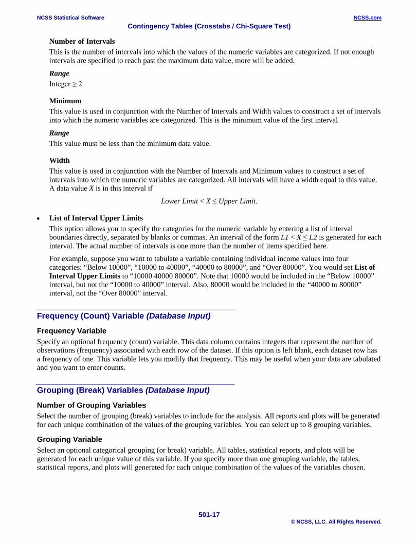
Number of Intervals This is the number of intervals into which the values of the numeric variables are categorized. If not enough intervals are specified to reach past the maximum data value, more will be added.
Range Integer ≥ 2
Minimum This value is used in conjunction with the Number of Intervals and Width values to construct a set of intervals into which the numeric variables are categorized. This is the minimum value of the first interval.
Range This value must be less than the minimum data value.
Width This value is used in conjunction with the Number of Intervals and Minimum values to construct a set of intervals into which the numeric variables are categorized. All intervals will have a width equal to this value. A data value X is in this interval if
Lower Limit < X ≤ Upper Limit.
• List of Interval Upper Limits This option allows you to specify the categories for the numeric variable by entering a list of interval boundaries directly, separated by blanks or commas. An interval of the form L1 < X ≤ L2 is generated for each interval. The actual number of intervals is one more than the number of items specified here.
For example, suppose you want to tabulate a variable containing individual income values into four categories: “Below 10000”, “10000 to 40000”, “40000 to 80000”, and “Over 80000”. You would set List of Interval Upper Limits to “10000 40000 80000”. Note that 10000 would be included in the “Below 10000” interval, but not the “10000 to 40000” interval. Also, 80000 would be included in the “40000 to 80000” interval, not the “Over 80000” interval.
Frequency (Count) Variable (Database Input)
Frequency Variable Specify an optional frequency (count) variable. This data column contains integers that represent the number of observations (frequency) associated with each row of the dataset. If this option is left blank, each dataset row has a frequency of one. This variable lets you modify that frequency. This may be useful when your data are tabulated and you want to enter counts.
Grouping (Break) Variables (Database Input)
Number of Grouping Variables Select the number of grouping (break) variables to include for the analysis. All reports and plots will be generated for each unique combination of the values of the grouping variables. You can select up to 8 grouping variables.
Grouping Variable Select an optional categorical grouping (or break) variable. All tables, statistical reports, and plots will be generated for each unique value of this variable. If you specify more than one grouping variable, the tables, statistical reports, and plots will generated for each unique combination of the values of the variables chosen.
NCSS Statistical Software NCSS.com Contingency Tables (Crosstabs / Chi-Square Test)
501-18 © NCSS, LLC. All Rights Reserved.
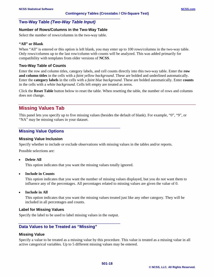
Two-Way Table (Two-Way Table Input)
Number of Rows/Columns in the Two-Way Table Select the number of rows/columns in the two-way table.
“All” or Blank When “All” is entered or this option is left blank, you may enter up to 100 rows/columns in the two-way table. Only rows/columns up to the last row/column with counts will be analyzed. This was added primarily for compatibility with templates from older versions of NCSS.
Two-Way Table of Counts Enter the row and column titles, category labels, and cell counts directly into this two-way table. Enter the row and column titles in the cells with a faint yellow background. These are bolded and underlined automatically. Enter the category labels in the cells with a faint blue background. These are bolded automatically. Enter counts in the cells with a white background. Cells left empty are treated as zeros.
Click the Reset Table button below to reset the table. When resetting the table, the number of rows and columns does not change.
Missing Values Tab This panel lets you specify up to five missing values (besides the default of blank). For example, “0”, “9”, or “NA” may be missing values in your dataset.
Missing Value Options
Missing Value Inclusion Specify whether to include or exclude observations with missing values in the tables and/or reports.
Possible selections are:
• Delete All This option indicates that you want the missing values totally ignored.
• Include in Counts This option indicates that you want the number of missing values displayed, but you do not want them to influence any of the percentages. All percentages related to missing values are given the value of 0.
• Include in All This option indicates that you want the missing values treated just like any other category. They will be included in all percentages and counts.
Label for Missing Values Specify the label to be used to label missing values in the output.
Data Values to be Treated as “Missing”
Missing Value Specify a value to be treated as a missing value by this procedure. This value is treated as a missing value in all active categorical variables. Up to 5 different missing values may be entered.
NCSS Statistical Software NCSS.com Contingency Tables (Crosstabs / Chi-Square Test)
501-19 © NCSS, LLC. All Rights Reserved.
Reports Tab This tab controls which tables and statistical reports are displayed in the output.
Select Reports
Data Summary Report Check this option to display a report of the summarized data for each combination of row and column variables across all break variables.
Contingency Tables
Show Individual Tables Check this option to display a separate table for each table statistic. After activating this option, you must specify which tables you would like to display.
The tables to choose from are:
• Counts • Table Percentages • Row Percentages • Column Percentages • Expected Counts Assuming Independence • Chi-Square Contributions • Deviations from Independence • Standardized Residuals
Show Combined Table Check this option to display a single table containing the selected statistics. After activating this option, you must specify which items you would like to display in the table.
The items to choose from are:
• Counts • Table Percentages • Row Percentages • Column Percentages • Expected Counts Assuming Independence • Chi-Square Contributions • Deviations from Independence • Standardized Residuals
Table Statistics and Tests
Tests for Row-Column Independence Check this option to output the “Tests for Row-Column Independence” report. These tests are used to test for independence between rows and columns of the table. Independence means that knowing the value of the row variable does not change the probabilities of the column variable (and vice versa). Another way of looking at independence is to say that the row percentages (or column percentages) remain constant from row to row (or column to column).

NCSS Statistical Software NCSS.com Contingency Tables (Crosstabs / Chi-Square Test)
501-20 © NCSS, LLC. All Rights Reserved.
When this option is checked, you will have the option of choosing from 4 different independence tests:
• Pearson’s Chi-Square Test Check this option to output Pearson’s Chi-Square Test for row-column independence.
This test requires large sample sizes to be accurate. An often quoted rule of thumb regarding sample size is that none of the expected cell values can be less than five. Although some users ignore the sample size requirement, you should be very skeptical of the test if you have cells in your table with zero counts. When these assumptions are violated, you should use Yates’ Continuity Corrected Test or Fisher’s Exact Test.
• Yates’ Continuity Corrected Chi-Square Test [2 × 2 Tables] Check this option to output Yates’ Continuity Corrected Chi-Square Test for row-column independence. This test is similar to Pearson's chi-square test, but is adjusted for the continuity of the chi-square distribution. This test is particularly useful when you have small sample sizes. This test is only calculated for 2 × 2 tables.
• Likelihood Ratio Test Check this option to output the Likelihood Ratio Test for row-column independence. This test makes use of the fact that under the null hypothesis of independence, the likelihood ratio statistic follows an asymptotic chi-square distribution.
• Fisher's Exact Test [2 × 2 Tables] Check this option to output the Fisher's Exact Test for row-column independence. Using the hypergeometric distribution with fixed row and column totals, this test computes probabilities of all possible tables with the observed row and column totals. This test is often used when sample sizes are small, but it is appropriate for all sample sizes. This test is only calculated for 2 × 2 tables.
Tests for Trend in Proportions [2 × k Tables] Check this option to output the various trend test reports. These tests are used to test for trend in proportions. These tests are only calculated for 2 × k tables. After selecting this option, you must select which trend tests to output. The options are
• Cochran-Armitage Test Check this option to output the Cochran-Armitage test for linear trend in proportions. The test may be used when you have exactly two rows or two columns in your table. This procedure tests the hypothesis that there is a linear trend in the proportion of successes. That is, the true proportion of successes increases (or decreases) as you move from row to row (or column to column). This test is only calculated for 2 × k tables.
The Cochran-Armitage Test is the most widely-used test for trend in proportions.
• Cochran-Armitage Test with Continuity Correction Check this option to output the Continuity Corrected Cochran-Armitage test for linear trend in proportions. In this test, Z-values are adjusted by the factor Δ/2, where Δ is the average distance between scores. The test may be used when you have exactly two rows or two columns in your table. This procedure tests the hypothesis that there is a linear trend in the proportion of successes. That is, the true proportion of successes increases (or decreases) as you move from row to row (or column to column). This test is only calculated for 2 × k tables.
• Armitage Rank Correlation Test Check this option to output the Armitage rank correlation test for trend in proportions. The test may be used when you have exactly two rows or two columns in your table. This procedure tests the hypothesis that there is a trend in the proportion of successes. That is, the true proportion of successes increases (or decreases) as you move from row to row (or column to column). This test is only calculated for 2 × k tables.
NCSS Statistical Software NCSS.com Contingency Tables (Crosstabs / Chi-Square Test)
501-21 © NCSS, LLC. All Rights Reserved.
McNemar Test [k × k Tables] Check this option to output the McNemar Test. The McNemar test was first used to compare two proportions that are based on matched samples. Matched samples occur when individuals (or matched pairs) are given two different treatments, asked two different questions, or measured in the same way at two different points in time. Match pairs can be obtained by matching individuals on several other variables, by selecting two people from the same family (especially twins), or by dividing a piece of material in half.
The McNemar test has been extended so that the measured variable can have more than two possible outcomes. It is then called the McNemar test of symmetry. It tests for symmetry around the diagonal of the table. The diagonal elements of the table are ignored. This test is only calculated for square k × k tables.
Kappa and Weighted Kappa Tests for Inter-Rater Agreement [k × k Tables] Check this option to output the Kappa Estimation and Hypothesis Tests reports. Kappa is a measure of association (correlation or reliability) between two measurements on the same individual when the measurements are categorical. It tests if the counts along the diagonal are significantly large. Because Kappa is used when the same variable is measured twice, it is only appropriate for square tables where the row and columns have the same categories. Kappa is often used to study the agreement of two raters such as judges or doctors. Each rater classifies each individual into one of k categories.
Rules-of-thumb for kappa: values less than 0.40 indicate low association; values between 0.40 and 0.75 indicate medium association; and values greater than 0.75 indicate high association between the two raters.
The items estimated and tested in the Kappa reports are
• Kappa • Weighted Kappa (With Linear and Quadratic Weights) • Maximum Kappa • Maximum-Adjusted Kappa
This report is only output for square k × k tables with identical row and column categories.
Weighted Kappa Weighted Kappa should only be used when the rater categories are ordered (e.g. “Low, Medium, High” or “1, 2, 3, 4”). The procedure applies weights to quantify relative distances between categories. These weights can be calculated as either linear or quadratic. Results from both are given in the report.
For 2 × 2 tables, Weighted Kappa is the same as simple Kappa.
Confidence Level This confidence level is used for the kappa and weighted kappa confidence intervals. Typical confidence levels are 90%, 95%, and 99%, with 95% being the most common.
Association and Correlation Statistics Check this option to output various categorical association and correlation statistics.
• Phi A measure of association independent of the sample size. Phi ranges between 0 (no relationship) and 1 (perfect relationship). Phi was designed for 2 × 2 tables only. For larger tables, it has no upper limit and Cramer’s V should be used instead.
• Cramer’s V A measure of association independent of sample size. This statistic is a modification of the Phi statistic so that it is appropriate for larger than 2 × 2 tables. Cramer’s V ranges between 0 (no relationship) and 1 (perfect relationship).

NCSS Statistical Software NCSS.com Contingency Tables (Crosstabs / Chi-Square Test)
501-22 © NCSS, LLC. All Rights Reserved.
• Pearson’s Contingency Coefficient A measure of association independent of sample size. It ranges between 0 (no relationship) and 1 (perfect relationship). For any particular table, the maximum possible depends on the size of the table (a 2 × 2 table has a maximum of 0.707), so it should only be used to compare tables with the same dimensions.
• Tschuprow’s T A measure of association independent of sample size. This statistic is a modification of the Phi statistic so that it is appropriate for larger than 2 × 2 tables. T ranges between 0 (no relationship) and 1 (perfect relationship), but 1 is only attainable for square tables.
• Lambda This is a measure of association for cross tabulations of nominal-level variables. It measures the percentage improvement in predictability of the dependent variable (row variable or column variable), given the value of the other variable (column variable or row variable).
• Kendall’s tau This is a measure of correlation between two ordinal-level (rankable) variables. It is most appropriate for square tables.
• Gamma This is another measure based on concordant and discordant pairs. It is appropriate only when both row and column variables are ordinal.
Alpha for Tests
Alpha Alpha is the significance level used in the hypothesis tests. A value of 0.05 is most commonly used, but 0.1, 0.025, 0.01, and other values are sometimes used. Typical values range from 0.001 to 0.20.
Report Options Tab The following options control the format of the reports.
Report Options
Variable Names Specify whether to use variable names, variable labels, or both to label output reports. In this discussion, the variables are the columns of the data table.
• Names Variable names are the column headings that appear on the data table. They may be modified by clicking the Column Info button on the Data window or by clicking the right mouse button while the mouse is pointing to the column heading.
• Labels This refers to the optional labels that may be specified for each column. Clicking the Column Info button on the Data window allows you to enter them.
• Both Both the variable names and labels are displayed.
NCSS Statistical Software NCSS.com Contingency Tables (Crosstabs / Chi-Square Test)
501-23 © NCSS, LLC. All Rights Reserved.
Comments 1. Most reports are formatted to receive about 12 characters for variable names.
2. Variable Names cannot contain blanks or math symbols (like + - * / . ,), but variable labels can.
Value Labels Value Labels are used to make reports more legible by assigning meaningful labels to numbers and codes.
The options are
• Data Values All data are displayed in their original format, regardless of whether a value label has been set or not.
• Value Labels All values of variables that have a value label variable designated are converted to their corresponding value label when they are output. This does not modify their value during computation.
• Both Both data value and value label are displayed.
Example A variable named GENDER (used as a grouping variable) contains 1’s and 2’s. By specifying a value label for GENDER, the report can display “Male” instead of 1 and “Female” instead of 2. This option specifies whether (and how) to use the value labels.
Table Formatting
Column Justification Specify whether data columns in the contingency tables will be left or right justified.
Column Widths Specify how the widths of columns in the contingency tables will be determined.
The options are
• Autosize to Minimum Widths Each data column is individually resized to the smallest width required to display the data in the column. This usually results in columns with different widths. This option produces the most compact table possible, displaying the most data per page.
• Autosize to Equal Minimum Width The smallest width of each data column is calculated and then all columns are resized to the width of the widest column. This results in the most compact table possible where all data columns have the same width. This is the default setting.
• Custom (User-Specified) Specify the widths (in inches) of the columns directly instead of having the software calculate them for you.
Custom Widths (Single Value or List) Enter one or more values for the widths (in inches) of columns in the contingency tables. This option is only displayed if Column Widths is set to “Custom (User-Specified)”.
NCSS Statistical Software NCSS.com Contingency Tables (Crosstabs / Chi-Square Test)
501-24 © NCSS, LLC. All Rights Reserved.
• Single Value If you enter a single value, that value will be used as the width for all data columns in the table.
• List of Values Enter a list of values separated by spaces corresponding to the widths of each column. The first value is used for the width of the first data column, the second for the width of the second data column, and so forth. Extra values will be ignored. If you enter fewer values than the number of columns, the last value in your list will be used for the remaining columns.
Type the word “Autosize” for any column to cause the program to calculate it's width for you. For example, enter “1 Autosize 0.7” to make column 1 be 1 inch wide, column 2 be sized by the program, and column 3 be 0.7 inches wide.
Wrap Column Headings onto Two Lines Check this option to make column headings wrap onto two lines. Use this option to condense your table when your data are spaced too far apart because of long column headings.
Decimal Places
Item Decimal Places These decimal options allow the user to specify the number of decimal places for items in the output. Your choice here will not affect calculations; it will only affect the format of the output.
• Auto If one of the “Auto” options is selected, the ending zero digits are not shown. For example, if “Auto (0 to 7)” is chosen,
0.0500 is displayed as 0.05 1.314583689 is displayed as 1.314584
The output formatting system is not designed to accommodate “Auto (0 to 13)”, and if chosen, this will likely lead to lines that run on to a second line. This option is included, however, for the rare case when a very large number of decimals is needed.
Omit Percent Sign after Percentages The program normally adds a percent sign, %, after each percentage. Checking this option will cause this percent sign to be omitted.

NCSS Statistical Software NCSS.com Contingency Tables (Crosstabs / Chi-Square Test)
501-25 © NCSS, LLC. All Rights Reserved.
Plots Tab The options on this panel allow you to select and control the appearance of the plots output by this procedure.
Select Plots
Show Plots Check this option to display a separate plot for each table statistic. After activating this option, you must specify which plots you would like to display.
The plots to choose from are:
• Counts • Table Percentages • Row Percentages • Column Percentages • Expected Counts Assuming Independence • Chi-Square Contributions • Deviations from Independence • Standardized Residuals Click the plot format button to change the plot display settings.
Show Break as Title Specify whether to display the values of the break variables as the second title line on the plots.
NCSS Statistical Software NCSS.com Contingency Tables (Crosstabs / Chi-Square Test)
501-26 © NCSS, LLC. All Rights Reserved.
Example 1 – 2 × 2 Contingency Table and Statistics from Raw Categorical Data The data for this example are found in the “CrossTabs1” dataset. This dataset contains fictitious survey data from 100 individuals asked about their sugar intake and exercise. Notice that we have entered custom value orders for the columns in the dataset so that the values will appear in the correct order. We use a 2 × 2 contingency table for this example so that all of the tests for row-column independence will be displayed.
You may follow along here by making the appropriate entries or load the completed template Example 1 by clicking on Open Example Template from the File menu of the Contingency Tables (Crosstabs / Chi-Square Test) window.
1 Open the CrossTabs1 dataset. • From the File menu of the NCSS Data window, select Open Example Data. • Click on the file CrossTabs1.NCSS. • Click Open.
2 Open the Contingency Tables (Crosstabs / Chi-Square Test) window. • Using the Analysis menu or the Procedure Navigator, find and select the Contingency Tables (Crosstabs
/ Chi-Square Test) procedure. • On the menus, select File, then New Template. This will fill the procedure with the default template.
3 Specify the variables. • Select the Variables tab. • For Type of Data Input select Columns in the Database. • Double-click in the Row Variable(s) text box. This will bring up the variable selection window. • Select Sugar from the list of variables and then click OK. “Sugar” will appear in the Row Variable(s)
box. • Double-click in the Column Variable(s) text box. This will bring up the variable selection window. • Select Exercise from the list of variables and then click OK. “Exercise” will appear in the Column
Variable(s) box.
4 Specify the reports. • Select the Reports tab. • Leave Show Individual Tables and Counts checked. • Check Show Combined Table and leave the selected table items checked. • Leave Tests for Row-Column Independence and the selected tests checked. • Check Association and Correlation Statistics.
5 Specify the plots. • Select the Plots tab. • Check Show Plots and leave Counts checked.
6 Run the procedure. • From the Run menu, select Run Procedure. Alternatively, just click the green Run button.
The following reports and plots will be displayed in the Output window.

NCSS Statistical Software NCSS.com Contingency Tables (Crosstabs / Chi-Square Test)
501-27 © NCSS, LLC. All Rights Reserved.
Output
Counts Table Exercise Sugar Infrequent Frequent Total Low 19 28 47 High 37 16 53 Total 56 44 100 Combined Table Exercise Sugar Infrequent Frequent Total Low Count 19 28 47 % of Total 19.00% 28.00% 47.00% % within Row 40.43% 59.57% 100.00% % within Column 33.93% 63.64% 47.00% High Count 37 16 53 % of Total 37.00% 16.00% 53.00% % within Row 69.81% 30.19% 100.00% % within Column 66.07% 36.36% 53.00% Total Count 56 44 100 % of Total 56.00% 44.00% 100.00% % within Row 56.00% 44.00% 100.00% % within Column 100.00% 100.00% 100.00% Tests for Row-Column Independence (Sugar by Exercise) H0: "Sugar" and "Exercise" are independent. H1: "Sugar" and "Exercise" are associated (not independent). Chi-Square Prob Reject H0 Test Type Value DF Level at α = 0.05? Pearson's Chi-Square 2-Sided 8.7299 1 0.00313 Yes Yates' Cont. Correction 2-Sided 7.5780 1 0.00591 Yes Likelihood Ratio 2-Sided 8.8440 1 0.00294 Yes Fisher's Exact 2-Sided 0.00458 Yes Fisher's Exact (Lower) 1-Sided 0.00284 Yes Fisher's Exact (Upper) 1-Sided 0.99926 No Association and Correlation Statistics (Sugar by Exercise) Statistic Value Phi 0.2955 Cramer's V 0.2955 Pearson's Contingency Coefficient 0.2834 Tschuprow's T 0.2955 Lambda A .. Rows dependent 0.2553 Lambda B .. Columns dependent 0.2045 Symmetric Lambda 0.2308 Kendall's tau-B -0.1479 Kendall's tau-B (with correction for ties) -0.2955 Kendall's tau-C -0.2928 Gamma -0.5463

NCSS Statistical Software NCSS.com Contingency Tables (Crosstabs / Chi-Square Test)
501-28 © NCSS, LLC. All Rights Reserved.
Plots Section (Sugar by Exercise)
This report presents the individual contingency table of counts, a combined table with counts and percentages, the results of the various row-column independence tests, and various association and correlation statistics. A plot of the counts is also displayed. The Pearson’s chi-square test results indicate that for these hypothetical data there is an association between a person’s sugar intake and exercise frequency (p-value = 0.00313).
NCSS Statistical Software NCSS.com Contingency Tables (Crosstabs / Chi-Square Test)
501-29 © NCSS, LLC. All Rights Reserved.
Example 2 – 3 × 4 Contingency Table and Statistics from Summarized Categorical Data The data for this example are found in the “CrossTabs2” dataset. Notice that we have entered custom value orders for the column labeled Region so that the values will appear in the correct order.
You may follow along here by making the appropriate entries or load the completed template Example 2a by clicking on Open Example Template from the File menu of the Contingency Tables (Crosstabs / Chi-Square Test) window.
1 Open the CrossTabs2 dataset. • From the File menu of the NCSS Data window, select Open Example Data. • Click on the file CrossTabs2.NCSS. • Click Open.
2 Open the Contingency Tables (Crosstabs / Chi-Square Test) window. • Using the Analysis menu or the Procedure Navigator, find and select the Contingency Tables (Crosstabs
/ Chi-Square Test) procedure. • On the menus, select File, then New Template. This will fill the procedure with the default template.
3 Specify the variables. • Select the Variables tab. • For Type of Data Input select Columns in the Database. • Double-click in the Row Variable(s) text box. This will bring up the variable selection window. • Select Region from the list of variables and then click OK. “Region” will appear in the Row Variable(s)
box. • Double-click in the Column Variable(s) text box. This will bring up the variable selection window. • Select Choice from the list of variables and then click OK. “Choice” will appear in the Column
Variable(s) box. • Double-click in the Frequency Variable text box. This will bring up the variable selection window. • Select Count from the list of variables and then click OK. “Count” will appear in the Frequency
Variable box.
4 Specify the reports. • Select the Reports tab. • Uncheck Show Individual Tables. • Check Show Combined Table and leave the selected table items checked. • Leave Tests for Row-Column Independence and the selected tests checked.
5 Specify the plots. • Select the Plots tab. • Check Show Plots and leave Counts checked.
6 Run the procedure. • From the Run menu, select Run Procedure. Alternatively, just click the green Run button.
The following reports and plots will be displayed in the Output window.

NCSS Statistical Software NCSS.com Contingency Tables (Crosstabs / Chi-Square Test)
501-30 © NCSS, LLC. All Rights Reserved.
Output
Combined Table Choice Region A B C D Total East Count 56 14 12 22 104 % of Total 20.59% 5.15% 4.41% 8.09% 38.24% % within Row 53.85% 13.46% 11.54% 21.15% 100.00% % within Column 62.22% 32.56% 26.09% 23.66% 38.24% West Count 15 27 8 24 74 % of Total 5.51% 9.93% 2.94% 8.82% 27.21% % within Row 20.27% 36.49% 10.81% 32.43% 100.00% % within Column 16.67% 62.79% 17.39% 25.81% 27.21% South Count 19 2 26 47 94 % of Total 6.99% 0.74% 9.56% 17.28% 34.56% % within Row 20.21% 2.13% 27.66% 50.00% 100.00% % within Column 21.11% 4.65% 56.52% 50.54% 34.56% Total Count 90 43 46 93 272 % of Total 33.09% 15.81% 16.91% 34.19% 100.00% % within Row 33.09% 15.81% 16.91% 34.19% 100.00% % within Column 100.00% 100.00% 100.00% 100.00% 100.00% Tests for Row-Column Independence (Region by Choice) H0: "Region" and "Choice" are independent. H1: "Region" and "Choice" are associated (not independent). Chi-Square Prob Reject H0 Test Type Value DF Level at α = 0.05? Pearson's Chi-Square† 2-Sided 75.3662 6 0.00000 Yes Yates' Cont. Correction* Likelihood Ratio 2-Sided 75.0616 6 0.00000 Yes Fisher's Exact* † WARNING: At least one cell had a value less than 5. * Test computed only for 2×2 tables. Plots Section (Region by Choice)
This report presents the results from the summarized data. The Pearson’s chi-square test results indicate that the row and column variables are not independent (p-value = 0.00000), but there is a sample size warning that should be considered. Note that Fisher’s Exact Test and Yates’ Continuity Correction are not reported because this is not a 2 × 2 table.
NCSS Statistical Software NCSS.com Contingency Tables (Crosstabs / Chi-Square Test)
501-31 © NCSS, LLC. All Rights Reserved.
An alternate way to enter this summarized data is to set Type of Data Input to Two-Way Table. You may follow along here by making the appropriate modifications to the current settings or load the completed template Example 2b by clicking on Open Example Template from the File menu of the Contingency Tables (Crosstabs / Chi-Square Test) window.
7 Modify the Data Input Type. • Select the Variables tab. • For Type of Data Input, select Two-Way Table. • For Rows, enter 3. • For Columns, enter 4. • Enter the titles, labels, and counts into the two-way table on the input window.
8 Run the procedure again. • From the Run menu, select Run Procedure. Alternatively, just click the green Run button.
The output will be exactly the same as that displayed above.
NCSS Statistical Software NCSS.com Contingency Tables (Crosstabs / Chi-Square Test)
501-32 © NCSS, LLC. All Rights Reserved.
Example 3 – 6 × 4 Contingency Table and Statistics from Raw Numeric Data The real estate data for this example are found in the “Resale” dataset. We’ll use the crosstabs procedure to create a table with city as the row variable and price groups as the column variable. The software will summarize the continuous price variable for us using a list of price group boundaries. We’ll use the column labels and value labels in the dataset to make the data easier to interpret in the reports.
You may follow along here by making the appropriate entries or load the completed template Example 3 by clicking on Open Example Template from the File menu of the Contingency Tables (Crosstabs / Chi-Square Test) window.
1 Open the Resale dataset. • From the File menu of the NCSS Data window, select Open Example Data. • Click on the file Resale.NCSS. • Click Open.
2 Open the Contingency Tables (Crosstabs / Chi-Square Test) window. • Using the Analysis menu or the Procedure Navigator, find and select the Contingency Tables (Crosstabs
/ Chi-Square Test) procedure. • On the menus, select File, then New Template. This will fill the procedure with the default template.
3 Specify the variables. • Select the Variables tab. • For Type of Data Input select Columns in the Database. • Double-click in the Row Variable(s) text box. This will bring up the variable selection window. • Select City from the list of variables and then click OK. “City” will appear in the Row Variable(s) box. • Clear the value in the Column Variable(s) text box so that the box is empty. • Check Create Other Column Variables from Numeric Data. • Double-click in the Numeric Variable(s) to Categorize for Use in Table Columns text box. This will
bring up the variable selection window. • Select Price from the list of variables and then click OK. “Price” will appear in the Numeric Variable(s)
to Categorize for Use in Table Columns box. • For Group Numeric Data into Categories Using select List of Interval Upper Limits. • For List enter 100000 200000 300000.
4 Specify the reports. • Select the Reports tab. • Leave Show Individual Tables and Counts checked. • Check Row Percentages under Show Individual Tables.
5 Specify the format. • Select the Report Options tab. • For Variable Names select Labels. • For Value Labels select Value Labels.
6 Run the procedure. • From the Run menu, select Run Procedure. Alternatively, just click the green Run button.
The following reports and plots will be displayed in the Output window.

NCSS Statistical Software NCSS.com Contingency Tables (Crosstabs / Chi-Square Test)
501-33 © NCSS, LLC. All Rights Reserved.
Output
Counts Table Sales Price Community Up To 100000 To 200000 To Over 100000 200000 300000 300000 Total Silverville 5 12 4 6 27 Los Wages 18 16 9 6 49 Red Gulch 5 3 3 1 12 Politicville 5 11 10 1 27 Senate City 6 12 4 2 24 Congresstown 2 4 2 3 11 Total 41 58 32 19 150 Row Percentages Table Sales Price Community Up To 100000 To 200000 To Over 100000 200000 300000 300000 Total Silverville 18.52% 44.44% 14.81% 22.22% 100.00% Los Wages 36.73% 32.65% 18.37% 12.24% 100.00% Red Gulch 41.67% 25.00% 25.00% 8.33% 100.00% Politicville 18.52% 40.74% 37.04% 3.70% 100.00% Senate City 25.00% 50.00% 16.67% 8.33% 100.00% Congresstown 18.18% 36.36% 18.18% 27.27% 100.00% Total 27.33% 38.67% 21.33% 12.67% 100.00% Tests for Row-Column Independence (Community by Sales Price) H0: "Community" and "Sales Price" are independent. H1: "Community" and "Sales Price" are associated (not independent). Chi-Square Prob Reject H0 Test Type Value DF Level at α = 0.05? Pearson's Chi-Square† 2-Sided 16.8045 15 0.33069 No Yates' Cont. Correction* Likelihood Ratio 2-Sided 16.2412 15 0.36620 No Fisher's Exact* † WARNING: At least one cell had an expected value less than 5. * Test computed only for 2×2 tables.
This report presents the results from the data with the continuous price variable grouped into 4 categories. The Pearson’s chi-square test results indicate that there is not enough evidence to conclude that the row and column variables are associated (p-value = 0.33069). There is an expected value warning that should be considered. Note that Fisher’s Exact Test and Yates’ Continuity Correction are not reported because this is not a 2 × 2 table.
NCSS Statistical Software NCSS.com Contingency Tables (Crosstabs / Chi-Square Test)
501-34 © NCSS, LLC. All Rights Reserved.
Example 4 – Tests for Trend in Proportions (Validation using Armitage (1955)) The data for this example come from Table 1 of Armitage (1955) and are stored in the “Armitage” dataset. The dataset contains counts of tonsil sizes (+, ++, +++) from 1398 children aged 0-15 years along with and indicator or whether each child is a carrier or non-carrier of the bacteria Streptococcus pyogenes. On page 378, Armitage (1955) calculates the Cochran-Armitage chi-square test statistic for the alternative hypothesis of any trend to be 7.19 on 1 df with a p-value of 0.007. On page 383, Armitage (1955) calculates the Rank Correlation Test chi-square test statistic for the alternative hypothesis of any trend to be 6.83 on 1 df with a p-value of 0.009.
You may follow along here by making the appropriate entries or load the completed template Example 4 by clicking on Open Example Template from the File menu of the Contingency Tables (Crosstabs / Chi-Square Test) window.
1 Open the Armitage dataset. • From the File menu of the NCSS Data window, select Open Example Data. • Click on the file Armitage.NCSS. • Click Open.
2 Open the Contingency Tables (Crosstabs / Chi-Square Test) window. • Using the Analysis menu or the Procedure Navigator, find and select the Contingency Tables (Crosstabs
/ Chi-Square Test) procedure. • On the menus, select File, then New Template. This will fill the procedure with the default template.
3 Specify the variables. • Select the Variables tab. • For Type of Data Input select Columns in the Database. • Double-click in the Row Variable(s) text box. This will bring up the variable selection window. • Select Strep from the list of variables and then click OK. “Strep” will appear in the Row Variable(s)
box. • Double-click in the Column Variable(s) text box. This will bring up the variable selection window. • Select Tonsils from the list of variables and then click OK. “Tonsils” will appear in the Column
Variable(s) box. • Double-click in the Frequency Variable text box. This will bring up the variable selection window. • Select Count from the list of variables and then click OK. “Count” will appear in the Frequency
Variable box.
4 Specify the reports. • Select the Reports tab. • Uncheck Show Individual Tables. • Check Show Combined Table and leave only Counts and Column Percentages checked. • Uncheck Tests for Row-Column Independence. • Check Tests for Trend in Proportions and all three corresponding trend tests.
5 Specify the report options. • Select the Report Options tab. • For Variable Names, select Labels.
6 Run the procedure. • From the Run menu, select Run Procedure. Alternatively, just click the green Run button.
The following reports and plots will be displayed in the Output window.

NCSS Statistical Software NCSS.com Contingency Tables (Crosstabs / Chi-Square Test)
501-35 © NCSS, LLC. All Rights Reserved.
Output
Combined Table Tonsil Size Streptococcus pyogenes 1 2 3 Total Non-carriers Count 497 560 269 1326 % within Column 96.32% 95.08% 91.81% 94.85% Carriers Count 19 29 24 72 % within Column 3.68% 4.92% 8.19% 5.15% Total Count 516 589 293 1398 % within Column 100.00% 100.00% 100.00% 100.00% Cochran-Armitage Trend Test (Streptococcus pyogenes by Tonsil Size) H0: p(1) = p(2) = p(3) = ... = p(k) Alternative Standard Prob Reject H0 Hypothesis* Numerator Error Z Level at α = 0.05? H1: Increasing Trend 16.48498 6.1467 2.6819 0.00366 Yes H1: Decreasing Trend 16.48498 6.1467 2.6819 0.99634 No H1: Any Trend 16.48498 6.1467 2.6819 0.00732 Yes * Trend is based on % within Column for Streptococcus pyogenes = "Carriers". Cochran-Armitage Trend Test with Continuity Correction (Streptococcus pyogenes by Tonsil Size) H0: p(1) = p(2) = p(3) = ... = p(k) Alternative Standard Prob Reject H0 Hypothesis* Numerator† Error Z Level at α = 0.05? H1: Increasing Trend 15.98498 6.1467 2.6006 0.00465 Yes H1: Decreasing Trend 15.98498 6.1467 2.6006 0.99535 No H1: Any Trend 15.98498 6.1467 2.6006 0.00931 Yes * Trend is based on % within Column for Streptococcus pyogenes = "Carriers". † Continuity Correction Factor (Δ/2) = 0.5 Armitage Rank Correlation Trend Test (Streptococcus pyogenes by Tonsil Size) H0: p(1) = p(2) = p(3) = ... = p(k) Alternative Numerator Standard Prob Reject H0 Hypothesis* S Error Z Level at α = 0.05? H1: Increasing Trend 16229 6208.3460 2.6141 0.00447 Yes H1: Decreasing Trend 16229 6208.3460 2.6141 0.99553 No H1: Any Trend 16229 6208.3460 2.6141 0.00895 Yes * Trend is based on % within Column for Streptococcus pyogenes = "Carriers".
The reported alternative hypotheses correspond to the trend in proportions for the second row (Strep = “Carriers”). The two-sided Cochran-Armitage test confirms that the carrier rate (% within Column for Strep = “Carriers”) does, in fact, change with the tonsil size (Z = 2.6819 and p-value = 0.00732). The continuity corrected test (p-value = 0.00931) and Armitage rank correlation test (Z = 2.6141 and p-value = 0.00895) show similar results. These test results match exactly those given in Armitage (1955) if we note that Z2 = Chi-Square on 1 df such that 2.68192=7.1926 and 2.61412=6.8335.

NCSS Statistical Software NCSS.com Contingency Tables (Crosstabs / Chi-Square Test)
501-36 © NCSS, LLC. All Rights Reserved.
Example 5 – McNemar Test The data for this example are found in the “McNemar” dataset. This hypothetical data contains summarized responses from 23 individuals who were asked about their desire to purchase a certain home-improvement product before and after a sales demonstration.
You may follow along here by making the appropriate entries or load the completed template Example 5 by clicking on Open Example Template from the File menu of the Contingency Tables (Crosstabs / Chi-Square Test) window.
1 Open the McNemar dataset. • From the File menu of the NCSS Data window, select Open Example Data. • Click on the file McNemar.NCSS. • Click Open.
2 Open the Contingency Tables (Crosstabs / Chi-Square Test) window. • Using the Analysis menu or the Procedure Navigator, find and select the Contingency Tables (Crosstabs
/ Chi-Square Test) procedure. • On the menus, select File, then New Template. This will fill the procedure with the default template.
3 Specify the variables. • Select the Variables tab. • For Type of Data Input select Columns in the Database. • Double-click in the Row Variable(s) text box. This will bring up the variable selection window. • Select Before from the list of variables and then click OK. “Before” will appear in the Row Variable(s)
box. • Double-click in the Column Variable(s) text box. This will bring up the variable selection window. • Select After from the list of variables and then click OK. “After” will appear in the Column Variable(s)
box. • Double-click in the Frequency Variable text box. This will bring up the variable selection window. • Select Count from the list of variables and then click OK. “Count” will appear in the Frequency
Variable box.
4 Specify the reports. • Select the Reports tab. • Leave Show Individual Tables and Counts checked. • Uncheck Tests for Row-Column Independence. • Check McNemar Test.
5 Run the procedure. • From the Run menu, select Run Procedure. Alternatively, just click the green Run button.
The following reports and plots will be displayed in the Output window.

NCSS Statistical Software NCSS.com Contingency Tables (Crosstabs / Chi-Square Test)
501-37 © NCSS, LLC. All Rights Reserved.
Output
Counts Table After Before No Yes Total No 6 10 16 Yes 3 4 7 Total 9 14 23 McNemar Test (Before by After) H0: P12 = P21 H1: P12 ≠ P21 Chi-Square Prob Reject H0 Test Type Value DF Level at α = 0.05? Asymptotic Chi-Square 2-Sided 3.7692 1 0.05220 No Binomial Exact 2-Sided 0.09229 No
Both the Asymptotic Chi-Square (p-value = 0.05220) and Binomial Exact (p-value = 0.09229) McNemar Tests indicate that there is not enough evidence to reject the null hypothesis.

NCSS Statistical Software NCSS.com Contingency Tables (Crosstabs / Chi-Square Test)
501-38 © NCSS, LLC. All Rights Reserved.
Example 6 – Kappa Test for Inter-Rater Agreement from Summarized Data (Validation using Fleiss, Levin, and Paik (2003)) Fleiss, Levin, and Paik (2003) present a hypothetical example on pages 598-608 in which 100 subjects are diagnosed independently by two raters and placed into 1 of 3 categories: Psychotic, Neurotic, and Organic. The summarized data are contained in the “KappaFleiss” dataset. In this example dataset, please note that a custom value order has been entered so that the table categories appear in the same order as in the book.
They compute a kappa value of 0.68, a null standard error of 0.076, and a z-value of 8.95 for testing the null hypothesis that kappa = 0. They also compute the asymptotic standard error for computing confidence intervals to be 0.087.
You may follow along here by making the appropriate entries or load the completed template Example 6a by clicking on Open Example Template from the File menu of the Contingency Tables (Crosstabs / Chi-Square Test) window.
1 Open the KappaFleiss dataset. • From the File menu of the NCSS Data window, select Open Example Data. • Click on the file KappaFleiss.NCSS. • Click Open.
2 Open the Contingency Tables (Crosstabs / Chi-Square Test) window. • Using the Analysis menu or the Procedure Navigator, find and select the Contingency Tables (Crosstabs
/ Chi-Square Test) procedure. • On the menus, select File, then New Template. This will fill the procedure with the default template.
3 Specify the variables. • Select the Variables tab. • For Type of Data Input select Columns in the Database. • Double-click in the Row Variable(s) text box. This will bring up the variable selection window. • Select Rater_A from the list of variables and then click OK. “Rater_A” will appear in the Row
Variable(s) box. • Double-click in the Column Variable(s) text box. This will bring up the variable selection window. • Select Rater_B from the list of variables and then click OK. “Rater_B” will appear in the Column
Variable(s) box. • Double-click in the Frequency Variable text box. This will bring up the variable selection window. • Select Count from the list of variables and then click OK. “Count” will appear in the Frequency
Variable box.
4 Specify the reports. • Select the Reports tab. • Leave Show Individual Tables and Counts checked. • Uncheck Tests for Row-Column Independence. • Check Kappa and Weighted Kappa Tests for Inter-Rater Agreement.
5 Run the procedure. • From the Run menu, select Run Procedure. Alternatively, just click the green Run button.
The following reports and plots will be displayed in the Output window.
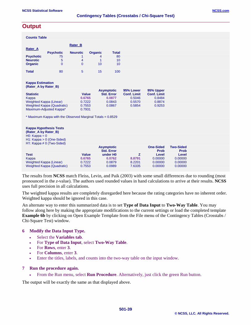
NCSS Statistical Software NCSS.com Contingency Tables (Crosstabs / Chi-Square Test)
501-39 © NCSS, LLC. All Rights Reserved.
Output
Counts Table Rater_B Rater_A Psychotic Neurotic Organic Total Psychotic 75 1 4 80 Neurotic 5 4 1 10 Organic 0 0 10 10 Total 80 5 15 100 Kappa Estimation (Rater_A by Rater_B) Asymptotic 95% Lower 95% Upper Statistic Value Std. Error Conf. Limit Conf. Limit Kappa 0.6765 0.0877 0.5046 0.8484 Weighted Kappa (Linear) 0.7222 0.0843 0.5570 0.8874 Weighted Kappa (Quadratic) 0.7553 0.0867 0.5854 0.9253 Maximum-Adjusted Kappa* 0.7931 * Maximum Kappa with the Observed Marginal Totals = 0.8529 Kappa Hypothesis Tests (Rater_A by Rater_B) H0: Kappa = 0 H1: Kappa > 0 (One-Sided) H1: Kappa ≠ 0 (Two-Sided) Asymptotic One-Sided Two-Sided Std. Error Prob Prob Test Value under H0 Z Level Level Kappa 0.6765 0.0762 8.8791 0.00000 0.00000 Weighted Kappa (Linear) 0.7222 0.0879 8.2201 0.00000 0.00000 Weighted Kappa (Quadratic) 0.7553 0.0989 7.6335 0.00000 0.00000
The results from NCSS match Fleiss, Levin, and Paik (2003) with some small differences due to rounding (most pronounced in the z-value). The authors used rounded values in hand calculations to arrive at their results. NCSS uses full precision in all calculations. The weighted kappa results are completely disregarded here because the rating categories have no inherent order. Weighted kappa should be ignored in this case. An alternate way to enter this summarized data is to set Type of Data Input to Two-Way Table. You may follow along here by making the appropriate modifications to the current settings or load the completed template Example 6b by clicking on Open Example Template from the File menu of the Contingency Tables (Crosstabs / Chi-Square Test) window.
6 Modify the Data Input Type. • Select the Variables tab. • For Type of Data Input, select Two-Way Table. • For Rows, enter 3. • For Columns, enter 3. • Enter the titles, labels, and counts into the two-way table on the input window.
7 Run the procedure again. • From the Run menu, select Run Procedure. Alternatively, just click the green Run button.
The output will be exactly the same as that displayed above.
NCSS Statistical Software NCSS.com Contingency Tables (Crosstabs / Chi-Square Test)
501-40 © NCSS, LLC. All Rights Reserved.
Example 7 – Weighted Kappa Test from Raw Data with Missing Cell Combinations The data for this example are contained in the “WeightedKappa” dataset. This dataset contains independent ratings by 2 raters on 12 individuals. Each individual was scored on a scale of 1 to 5. The goal is to determine how closely the raters’ scores agree. Weighted kappa is appropriate in this case because the categories are ordinal, meaning that the categories have magnitude with natural ordering.
The problem with the data in this dataset, however, is that there are no cases where Rater 1 scored an individual as “3” and there are no cases where Rater 2 scored and individual as “2”. This results in a contingency table that is square, but does not have identical row and column categories. The second part of the example will show you how to modify the data by adding zeros appropriately so that kappa can be computed without having to go through the added step of summarizing the data first.
You may follow along here by making the appropriate entries or load the completed template Example 7a by clicking on Open Example Template from the File menu of the Contingency Tables (Crosstabs / Chi-Square Test) window.
1 Open the WeightedKappa dataset. • From the File menu of the NCSS Data window, select Open Example Data. • Click on the file WeightedKappa.NCSS. • Click Open.
2 Open the Contingency Tables (Crosstabs / Chi-Square Test) window. • Using the Analysis menu or the Procedure Navigator, find and select the Contingency Tables (Crosstabs
/ Chi-Square Test) procedure. • On the menus, select File, then New Template. This will fill the procedure with the default template.
3 Specify the variables. • Select the Variables tab. • For Type of Data Input select Columns in the Database. • Double-click in the Row Variable(s) text box. This will bring up the variable selection window. • Select Rater_1 from the list of variables and then click OK. “Rater_1” will appear in the Row
Variable(s) box. • Double-click in the Column Variable(s) text box. This will bring up the variable selection window. • Select Rater_2 from the list of variables and then click OK. “Rater_2” will appear in the Column
Variable(s) box.
4 Specify the reports. • Select the Reports tab. • Leave Show Individual Tables and Counts checked. • Uncheck Tests for Row-Column Independence. • Check Kappa and Weighted Kappa Tests for Inter-Rater Agreement.
5 Specify the format. • Select the Report Options tab. • For Variable Names select Labels.
6 Run the procedure. • From the Run menu, select Run Procedure. Alternatively, just click the green Run button.
The following reports and plots will be displayed in the Output window.

NCSS Statistical Software NCSS.com Contingency Tables (Crosstabs / Chi-Square Test)
501-41 © NCSS, LLC. All Rights Reserved.
Output
Counts Table Rater 2 Rater 1 1 3 4 5 Total 1 3 0 0 0 3 2 0 3 0 0 3 4 0 1 2 0 3 5 0 0 1 2 3 Total 3 4 3 2 12 The number of rows with at least one missing value is 1 Kappa Estimation (Rater 1 by Rater 2) Not Calculated: Kappa statistics are only calculated for square k×k tables with identical row and column categories. Kappa Hypothesis Tests (Rater 1 by Rater 2) Not Calculated: Kappa tests are only calculated for square k×k tables with identical row and column categories.
This report indicates that it is not possible to calculate the kappa test statistic for this table since the table categories are not identical for rows and columns. There is no row category “3” for Rater 1 and no column category “2” for Rater 2. This is a result of the fact that some categories were not applied by each rater. We could re-enter this summarized data into the data table, including missing rows and columns with assigned counts of “0”, but there is an easier way. Simply add a new variable “Count” to the dataset and give each row a count value of “1”. In the row immediately after the last data row, enter the values for each rater that were never observed (i.e. in the first empty row at the end of the dataset, enter “3” under Rater_1 and “2” under Rater_2) and assign those a count value of “0”. In the example dataset we created new variables RaterMod_1, RaterMod_2, and Count to illustrate this principle, but in your dataset you do not necessarily have to create new rater variables; you can just add the rows with count = 0 starting at the first empty row. We’ll now run the analysis using the modified variables to get the kappa results. You may follow along here by making the appropriate modifications to the current settings or load the completed template Example 7b by clicking on Open Example Template from the File menu of the Contingency Tables (Crosstabs / Chi-Square Test) window.
7 Modify the variables. • Select the Variables tab. • For Type of Data Input select Columns in the Database. • Double-click in the Row Variable(s) text box. This will bring up the variable selection window. • Select RaterMod_1 from the list of variables and then click OK. “RaterMod_1” will appear in the Row
Variable(s) box. • Double-click in the Column Variable(s) text box. This will bring up the variable selection window. • Select RaterMod_2 from the list of variables and then click OK. “RaterMod_2” will appear in the
Column Variable(s) box. • Double-click in the Frequency Variable text box. This will bring up the variable selection window. • Select Count from the list of variables and then click OK. “Count” will appear in the Frequency
Variable box.
8 Run the procedure again. • From the Run menu, select Run Procedure. Alternatively, just click the green Run button.
The following reports and plots will be displayed in the Output window.

NCSS Statistical Software NCSS.com Contingency Tables (Crosstabs / Chi-Square Test)
501-42 © NCSS, LLC. All Rights Reserved.
Output
Counts Table Rater 2 Rater 1 1 2 3 4 5 Total 1 3 0 0 0 0 3 2 0 0 3 0 0 3 3 0 0 0 0 0 0 4 0 0 1 2 0 3 5 0 0 0 1 2 3 Total 3 0 4 3 2 12 Kappa Estimation (Rater 1 by Rater 2) Asymptotic 95% Lower 95% Upper Statistic Value Std. Error Conf. Limit Conf. Limit Kappa 0.5000 0.1429 0.2199 0.7801 Weighted Kappa (Linear) 0.7561 0.0968 0.5664 0.9458 Weighted Kappa (Quadratic) 0.9057 0.0481 0.8114 0.9999 Maximum-Adjusted Kappa* 0.8333 * Maximum Kappa with the Observed Marginal Totals = 0.6000 Kappa Hypothesis Tests (Rater 1 by Rater 2) H0: Kappa = 0 H1: Kappa > 0 (One-Sided) H1: Kappa ≠ 0 (Two-Sided) Asymptotic One-Sided Std. Error Prob Two-Sided Test Value under H0 Z Level P-Value Kappa 0.5000 0.1173 4.2640 0.00001 0.00002 Weighted Kappa (Linear) 0.7561 0.1952 3.8725 0.00005 0.00011 Weighted Kappa (Quadratic) 0.9057 0.2856 3.1708 0.00076 0.00152
The counts table now has identical row and column categories with the exact same counts as the previous table. A row and column of zeros have been added to make the table suitable for the calculation of the kappa and weighted kappa statistics. It is appropriate to consider the weighted kappa statistic in this case because the data are comprised of ordered scores. A weighted kappa value of 0.7561 indicates moderate-to-high agreement between the raters. If we did not take into account the ordinal nature of the data and looked at the simple kappa statistic, we would conclude a much lower association of 0.5000. This demonstrates the importance of using weighted kappa when it is appropriate.
NCSS Statistical Software NCSS.com Contingency Tables (Crosstabs / Chi-Square Test)
501-43 © NCSS, LLC. All Rights Reserved.
Example 8 – Data Summary Report The data summary report was designed for situations in which you want to transfer a summarized table to another program. This format creates a vertical listing of the counts in a format that is easy to copy and paste into another NCSS dataset or into other programs. The data for this example are found in the “Resale” dataset.
You may follow along here by making the appropriate entries or load the completed template Example 8 by clicking on Open Example Template from the File menu of the Contingency Tables (Crosstabs / Chi-Square Test) window.
1 Open the Resale dataset. • From the File menu of the NCSS Data window, select Open Example Data. • Click on the file Resale.NCSS. • Click Open.
2 Open the Contingency Tables (Crosstabs / Chi-Square Test) window. • Using the Analysis menu or the Procedure Navigator, find and select the Contingency Tables (Crosstabs
/ Chi-Square Test) procedure. • On the menus, select File, then New Template. This will fill the procedure with the default template.
3 Specify the variables. • Select the Variables tab. • For Type of Data Input select Columns in the Database. • Double-click in the Row Variable(s) text box. This will bring up the variable selection window. • Select City from the list of variables and then click OK. “City” will appear in the Row Variable(s) box. • Clear the value in the Column Variable(s) text box so that the box is empty. • Check Create Other Column Variables from Numeric Data. • Double-click in the Numeric Variable(s) to Categorize for Use in Table Columns text box. This will
bring up the variable selection window. • Select Price from the list of variables and then click OK. “Price” will appear in the Numeric Variable(s)
to Categorize for Use in Table Columns box. • For Group Numeric Data into Categories Using select List of Interval Upper Limits. • For List enter 100000 200000 300000.
4 Specify the reports. • Select the Reports tab. • Check Data Summary Report. • Leave Show Individual Tables and Counts checked. • Uncheck Tests for Row-Column Independence.
5 Run the procedure. • From the Run menu, select Run Procedure. Alternatively, just click the green Run button.
The following reports and plots will be displayed in the Output window.
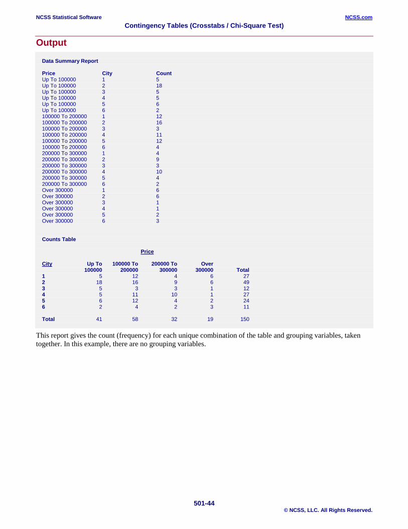
NCSS Statistical Software NCSS.com Contingency Tables (Crosstabs / Chi-Square Test)
501-44 © NCSS, LLC. All Rights Reserved.
Output
Data Summary Report Price City Count Up To 100000 1 5 Up To 100000 2 18 Up To 100000 3 5 Up To 100000 4 5 Up To 100000 5 6 Up To 100000 6 2 100000 To 200000 1 12 100000 To 200000 2 16 100000 To 200000 3 3 100000 To 200000 4 11 100000 To 200000 5 12 100000 To 200000 6 4 200000 To 300000 1 4 200000 To 300000 2 9 200000 To 300000 3 3 200000 To 300000 4 10 200000 To 300000 5 4 200000 To 300000 6 2 Over 300000 1 6 Over 300000 2 6 Over 300000 3 1 Over 300000 4 1 Over 300000 5 2 Over 300000 6 3 Counts Table Price City Up To 100000 To 200000 To Over 100000 200000 300000 300000 Total 1 5 12 4 6 27 2 18 16 9 6 49 3 5 3 3 1 12 4 5 11 10 1 27 5 6 12 4 2 24 6 2 4 2 3 11 Total 41 58 32 19 150
This report gives the count (frequency) for each unique combination of the table and grouping variables, taken together. In this example, there are no grouping variables.
Related Documents