Keller-Segel-Type Models and Kinetic Equations for Interacting Particles: Long-Time Asymptotic Analysis presented by Franca Karoline Olga HOFFMANN Member of Christ’s College University of Cambridge Centre for Mathematical Sciences Cambridge Centre for Analysis (CCA) submitted April 2017 Supervised by José Antonio Carrillo and Clément Mouhot This dissertation is submitted for the degree of Doctor of Philosophy (Mathematics).

Welcome message from author
This document is posted to help you gain knowledge. Please leave a comment to let me know what you think about it! Share it to your friends and learn new things together.
Transcript
Keller-Segel-Type Models and
Kinetic Equations
for Interacting Particles:
Long-Time Asymptotic Analysis
presented by
Franca Karoline Olga HOFFMANN
Member of Christ’s College
University of Cambridge
Centre for Mathematical Sciences
Cambridge Centre for Analysis (CCA)
submitted April 2017
Supervised by
José Antonio Carrillo and Clément Mouhot
This dissertation is submitted for the degree of
Doctor of Philosophy (Mathematics).

u Dissertation Summary U
Franca Karoline Olga HOFFMANN
Keller-Segel-Type Models and Kinetic Equations
for Interacting Particles: Long-Time Asymptotic Analysis
This thesis consists of three parts: The first and second parts focus on long-time asymptotics
of macroscopic and kinetic models respectively, while in the third part we connect these regimes
using different scaling approaches.
Keller–Segel-type aggregation-diffusion equations
We study a Keller–Segel-type model with non-linear power-law diffusion and non-local particle
interaction: Does the system admit equilibria? If yes, are they unique? Which solutions converge
to them? Can we determine an explicit rate of convergence? To answer these questions, we make
use of the special gradient flow structure of the equation and its associated free energy functional
for which the overall convexity properties are not known. Special cases of this family of models
have been investigated in previous works, and this part of the thesis represents a contribution to-
wards a complete characterisation of the asymptotic behaviour of solutions.
Hypocoercivity techniques for a fibre lay-down model
We show existence and uniqueness of a stationary state for a kinetic Fokker-Planck equationmod-
elling the fibre lay-down process in non-woven textile production. Further, we prove convergence
to equilibriumwith an explicit rate. This part of the thesis is an extension of previous work which
considered the case of a stationary conveyor belt. Adding the movement of the belt, the global
equilibrium state is not known explicitly and a more general hypocoercivity estimate is needed.
Although we focus here on a particular application, this approach can be used for any equation
with a similar structure as long as it can be understood as a certain perturbation of a system for
which the global Gibbs state is known.
Scaling approaches for collective animal behaviour models
We study the multi-scale aspects of self-organised biological aggregations using various scaling
techniques. Not many previous studies investigate how the dynamics of the initial models are
preserved via these scalings. Firstly, we consider two scaling approaches (parabolic and grazing
collision limits) that can be used to reduce a class of non-local kinetic 1D and 2Dmodels to simpler
models existing in the literature. Secondly, we investigate how some of the kinetic spatio-temporal
patterns are preserved via these scalings using asymptotic preserving numerical methods.
i


u Remerciements U
Mwanzo wa chanzo ni chane mbili...
It was at a seminar talk by Vincent Calvez one late afternoon in December 2011 at the ENS
Lyon that I first heard about the study of biological aggregation by means of partial differential
equations. I was amazed how very theoretical mathematical arguments from PDE Theory and
Functional Analysis can contribute directly to the understanding of complicated phenomena we
observe in nature. And I was fascinated by the videos of moving bands of E. coli . As the lecturer
of my first PDE course and guiding my first research steps in a summer internship, it was Vincent
who inspired my interest in PDE Analysis and who put me in touch with José Antonio Carrillo,
who then tookme on as a master student in the topic. Thanks to José Antonio’s enjoyable supervi-
sion style and his infectious passion for the subject, I stayed on for a PhD, co-supervised together
with Clément Mouhot at the University of Cambridge. I am extremely grateful to the Cambridge
Centre for Analysis (CCA), especially James Norris, for allowing me to pursue an unusual PhD
arrangement based jointly at University of Cambridge and Imperial College London under the
supervision of José Antonio and Clément. It is a real honour to work with these two great math-
ematicians, to learn from them, and to be part of their academic family.
It is thanks to Clément that I was able to stay in my cohort at the Cambridge Centre of Analysis
and be part of his very active research group in Cambridge, whilst continuing to work with José
Antonio in London. I am very grateful for his support and generosity during the years of my
thesis, for introducing me to the world of kinetic theory and passing on his enthusiasm for the
subject. Thank you for suggesting a research problem that I am passionate about, for making the
very enjoyable collaboration with Émeric Bouin possible and for handling many administrative
challenges related to my PhD arrangement.
Most of my thesis has been supervised by José Antonio, who has been a role model to me both on
an academic and on a personal level. His clairvoyance and problem solving skills (mathematical
and otherwise), as well as his pedagogical and organisational skills are exceptional. Discussions
with him are highly enjoyable and rewarding, his stamina to explain things is astounding, and
he always brings with him a positive attitude and a smile. He believes in the research abilities
of his students and sees them as actual assets, rather than burdens. I am 8-ly grateful for the
numerous opportunities that he provided during my PhD by suggesting collaborations, research
programs and conferences, inspiring me to take up an academic research career and fostering my
development towards amathematical globetrotter in the process. It is for good reasons that hewas
awarded the ’Best Supervision Award 2016’ by the Imperial College Union following our nomina-
tion, since, in Markus’ words, “he puts the super in supervisor”. I cannot thank you enough for all
iii

your time, your support, your mentorship, your availability, your patience and encouragements,
your open ear, for sharing your mathematical thought process in a way that is both inspiring and
educational, for your advice and help in navigating the academic world, for accepting to super-
vise me under several rather unconventional arrangements, for never stopping to believe in me,
for putting up with my sometimes crazy plans, interests and adventures (be it exchanging my of-
fice for a bus on a bumpy road in Kenya, being taken up by wardening duties, or trying Swedish
Surströmming), and thank you for making my PhD such an enjoyable experience.
Another person who has played a significant role for the shaping of this thesis and my decision to
continue in academia is Vincent Calvez. Thank you for being a great mentor, for all your support,
your encouragements and your patience, theywere invaluable. Thank you for taking care of me as
if I would be one of your own students and for giving me the possibility to return to the beautiful
city of Lyon so many times.
During the time of my PhD, I had the chance to meet, learn from and work with many talented
mathematicians that have shapedmy idea of what it means to be a researcher. It is through bounc-
ing off ideas, seeing a problem through somebody else’s eyes and being able to ask questions that
mathematics comes alive. As I’ve learned in Kenya:
Iwapo unataka kwenda haraka, nenda peke yako;
Iwapo mnataka kwenda mbali, nendeni pamoja.1
I’m especially grateful to my collaborators and mentors Raluca Eftimie, Émeric Bouin, Eric
Carlen, Jean Dolbeault, Bruno Volzone, EdoardoMainini and Peter Dobbins – thank you for fruit-
ful discussions, virtual and in front of blackboards, and for teaching me new interesting math-
ematics. Finally, I thank my examiners Adrien Blanchet and Carola Schönlieb, who accepted to
read all these words.
My time as a PhD student was an exciting, eventful, diverse, sometimes challenging, and
mostly enjoyable journey shaped by people from all around the globe. First of all, let me mention
my PhD brothers and sisters Francesco, Markus, Rafa and Sergio from the London side, and Lu-
dovic, Jo, Megan, Helge, Tom, Sara andMarc from the Cambridge side, my officemates in London
Marina, Marco, Tom, Sam, Nik, Onur, Maddy, Urbain, Anna, Cezary, Massi, Luca, Silvia andMar-
tin, and my fellow CCAers in Cambridge Adam, Harold, Karen, Ellen, Ben, David, Dominik, Da-
vide, Eavan and Sam, and the manymathematicians that I had the chance working, travelling and
conferencing with Pedro, Esther, Ewelina, Émeric, Amit, Ariane, Yao, Gaspard, Mikaela, Oliver,
Álvaro, Nils, José Alfredo, Simone, Young-Pil, Yanghong, Aneta, Claudia, Francesco, Anna, Gabi,
Katrin, Susanne ... and many others. The PhD ride was so much more enjoyable sharing it with
1If you want to go quickly, go alone; If you want to go far, go together.
iv
you, from all sorts of dinners to self-organised office seminars, spontaneous dancing sessions and
conference laser quest.
Further, thanks to the 2015-16 Imperial College SIAM chapter team Michael, Juvid, Hanne, Alex,
Adam, Marina and Arman, and the Imperial College Maths Helpdesk teamAlexis, Michael, Tom,
Isaac and Sam for all your enthusiasm and for putting up with me in so many meetings, not to
forget the resourceful Anderson Santos for battling Imperial College administration on our behalf
and always lending an open ear.
Turning the task of taking care of hundreds of freshers (trust me, a recommendable life train-
ing) into an enjoyable challenge, I was lucky to live with the most amazing warden teams João,
Arash, Mirko, Abi, Stu, Tas, Sei and Ben. You are my South Kensington family. Thanks to several
energetic warden and hall senior teams for uncountable 8 am meetings, dinners, parties, BBQs,
eventful freshers fortnights and for putting up with all my travel plans, (and yes, it’s a djembe, not
a bongo!).
A big influence on the kind of proverbs and quotes in this thesis comes from unforgettable mo-
ments spent on the African continent thanks to the amazing people of AMI and SAMI, and the
many volunteers from all around the world that put their time, brains, sweat and hearts into mak-
ingmaths camps and other educational initiatives happen acrossAfrica and in theUK. I’mgrateful
to have found you and to be part of this very inspiring network of people, you have changed my
view on theworld. And of course, all of this would have never been possible without José Antonio
and Clément being supportive of my different parallel lifes.
Last but not least, thanks to all the special people in my life who are always there for me, no
matterwhere, nomatterwhen, it is impossible to name you all, but you knowwho you are. I thank
my adopted families the Heepe-Sullivans and the Bichets who gave me a home away from home,
vous avez pour toujours une place très spéciale dans mon cœur. For their friendship and support
for many years, I am grateful to Ileana, Ronja Räubertochter, Natalia, Féfé, Terja, Céleste, Janine,
Judith, Dobriyana, Julie, Srinjan, Njoki, Wafa, Marina, Marco (pineapple on pizza?), toMarkus for
special party and Spätzle-making skills and his unbeatable sense of humour, and of course to my
beloved String Theory people. How could I ever forget the hours of music around mountains of
cheese only topped by Uruguayan asado? Thanks to Kin for helping me to keep up and progress
on the viola and for unforgettable duo performances in Lyon, Stockholm, London and Cambridge,
to Agustin Omwami for a unique goat experience and so much more, to David Stern for impor-
tant life advice, to Arieh Iserles for several philosphical coffees, to Juan Luis Vázquez Suárez for
perspicacious stories on the life as a mathematician, to my maths teacher Michael Mannheims for
his inspiring way of teaching, to our Mathe-LK of which certain people manage to generate, year
after year, entertaining Christmas stories, and to my kizomberos and salseros, who make sure I’m
v

staying (in)sane.
Wer mich am meisten zu Verrücktheiten inspiriert und mich davor bewahrt gar zu verrückt zu
werden ist meine Familie. Danke an Opa Jörg, der es immer wieder schafft, die Großfamilie
zusammen zu führen, an meine Eltern, die mir Flügel und einen sicheren Hafen schenken, an
meinen talentierten Bruder, unseren Fisch-Experten, der immer für mich da ist, an Lisa, an meine
Onkels und Cousinen mit Familie, die immer ein offenes Ohr für mich haben und mit denen ich
gerne mehr Zeit verbringen würde. Meine Familie hat es nach mehr oder weniger erfolgreichen
Erklärungsversuchen inzwischen aufgegegeben, zu verstehen, was ich nun eigentlich genau in
meiner Doktorarbeit erforsche, und dennoch geben sie mir immer neue Energie und Motivation.
Wie mein Papa so oft sagt, wenn er sieht wie ich Integrale auf’s Papier werfe: “Also, ich kann das
jetzt nur ästhetisch beurteilen...”
vi
u Statement of Originality U
I hereby declare that my dissertation entitled ’Keller-Segel-TypeModels and Kinetic Equations for
Interacting Particles: Long-Time Asymptotic Analysis’ is not substantially the same as any that I
have submitted, or, is being concurrently submitted for a degree or diploma or other qualifica-
tion at the University of Cambridge or any other University or similar institution. I further state
that no substantial part of my dissertation has already been submitted, or, is being concurrently
submitted for any such degree, diploma or other qualification at the University of Cambridge or
any other University or similar institution, except as declared in this text. This dissertation is the
result of my own work and includes nothing which is the outcome of work done in collaboration
except where specifically indicated in this text.
Chapter 1 motivates the research problems investigated in this thesis, gives an overview of the
mathematical methods and techniques that are relevant for Chapters 2-6, provides an overview
of the literature and states the main results of this thesis. The literature review was done under
the guidance, explanations and supervision of Professor José A. Carrillo2 and Professor Clément
Mouhot3.
The original research problem that led to the results in Part I (Chapters 2-4) was suggested by
Professor José A. Carrillo. Chapters 2 and 3 are original research work produced in collaboration
with Professor José A. Carrillo and Professor Vincent Calvez4. Chapter 4 is original research work
produced in collaboration with Professor José A. Carrillo, Professor Edoardo Mainini5 and Pro-
fessor Bruno Volzone6. Professor José A. Carrillo was the one who suggested the collaborations.
The radiality proof in Section 2.1 of Chapter 4 was contributed by Professor José A. Carrillo and
Professor Bruno Volzone, but has been included here for completeness.
Part II (Chapter 5) is original research work produced in collaboration with Professor Clément
Mouhot and Doctor Emeric Bouin7. Professor Clément Mouhot suggested the research problem
and the collaboration.
2Department of Mathematics, Imperial College London, South Kensington Campus, London SW7 2AZ, UK.3DPMMS, Centre for Mathematical Sciences, University of Cambridge, Wilberforce Road, Cambridge CB3 0WA, UK.4Unité de Mathématiques Pures et Appliquées, CNRS UMR 5669 and équipe-projet INRIA NUMED, École Normale
Supérieure de Lyon, Lyon, France.5Dipartimento di Ingegneria Meccanica, Università degli Studi di Genova, Genova, Italia.6Dipartimento di Ingegneria, Università degli Studi di Napoli “Parthenope”, Napoli, Italia.7CEREMADE - Université Paris-Dauphine, UMR CNRS 7534, Paris, France.
vii

Part III (Chapter 6) is original research work produced in collaboration with Professor José
A. Carrillo and Professor Raluca Eftimie8. The collaboration was suggested by Professor José A.
Carrillo. Section 2.2 in Chapter 6 was contributed by Professor Raluca Eftimie. Section 3.2 in
Chapter 6 was contributed by Professor José A. Carrillo. Some of the results presented in Chapter
6 were already part of my master thesis, namely: (1) a special case of Remark 2.2, (2) the parabolic
drift-diffusion limit in Section 3.1, and (3) a theoretical development of the AP scheme used in
Section 4, all for the case λ1 “ 0. These parts have been included in this dissertation to allow for
a comprehensive and self-contained presentation of Chapter 6.
8Division of Mathematics, University of Dundee, Dundee, UK.
viii

Dzigbodi wotso koa anyidi
dide hafi kpona efe doka.
If you patiently dissect an ant,
you will see its entrails 9.
Ghanaian proverb (Ewe)
9With patience, you can accomplish the most difficult task.
ix


Für Margarita & Freimut, meine Eltern,
die fast alle Verrücktheiten ihrer Tochter mitmachen
und mich bedingungslos unterstützen.
xi
Contents
1. Introduction 3
1 The Keller–Segel model . . . . . . . . . . . . . . . . . . . . . . . . . . . . . . . . . . . 8
2 Part I: Keller–Segel-type aggregation-diffusion equations . . . . . . . . . . . . . . . 10
3 Part I: Results . . . . . . . . . . . . . . . . . . . . . . . . . . . . . . . . . . . . . . . . 24
4 Part I: Perspectives . . . . . . . . . . . . . . . . . . . . . . . . . . . . . . . . . . . . . 42
5 Part II: Non-woven textiles . . . . . . . . . . . . . . . . . . . . . . . . . . . . . . . . . 46
6 Part II: Hypocoercivity . . . . . . . . . . . . . . . . . . . . . . . . . . . . . . . . . . . 50
7 Part II: Results . . . . . . . . . . . . . . . . . . . . . . . . . . . . . . . . . . . . . . . . 57
8 Part III: From micro to macro . . . . . . . . . . . . . . . . . . . . . . . . . . . . . . . 64
9 Part III: Collective animal behaviour . . . . . . . . . . . . . . . . . . . . . . . . . . . 70
I Keller-Segel-Type Aggregation-Diffusion Equations 77
2. Ground states in the fair-competition regime 79
1 Introduction . . . . . . . . . . . . . . . . . . . . . . . . . . . . . . . . . . . . . . . . . 81
2 Stationary states & main results . . . . . . . . . . . . . . . . . . . . . . . . . . . . . . 84
3 Porous medium case k ă 0 . . . . . . . . . . . . . . . . . . . . . . . . . . . . . . . . . 90
4 Fast diffusion case k ą 0 . . . . . . . . . . . . . . . . . . . . . . . . . . . . . . . . . . 110
A Appendix: Properties of ψk . . . . . . . . . . . . . . . . . . . . . . . . . . . . . . . . 120
3. Asymptotics in the one-dimensional fair-competition regime 129
1 Introduction . . . . . . . . . . . . . . . . . . . . . . . . . . . . . . . . . . . . . . . . . 131
2 Preliminaries . . . . . . . . . . . . . . . . . . . . . . . . . . . . . . . . . . . . . . . . . 136
3 Functional inequalities . . . . . . . . . . . . . . . . . . . . . . . . . . . . . . . . . . . 142
4 Long-time asymptotics . . . . . . . . . . . . . . . . . . . . . . . . . . . . . . . . . . . 153
5 Numerical simulations . . . . . . . . . . . . . . . . . . . . . . . . . . . . . . . . . . . 169
xii
Contents
6 Explorations in other regimes . . . . . . . . . . . . . . . . . . . . . . . . . . . . . . . 182
4. Ground states in the diffusion-dominated regime 189
1 Introduction . . . . . . . . . . . . . . . . . . . . . . . . . . . . . . . . . . . . . . . . . 191
2 Stationary states . . . . . . . . . . . . . . . . . . . . . . . . . . . . . . . . . . . . . . . 193
3 Global minimisers . . . . . . . . . . . . . . . . . . . . . . . . . . . . . . . . . . . . . . 198
4 Uniqueness in one dimension . . . . . . . . . . . . . . . . . . . . . . . . . . . . . . . 210
A Appendix: Properties of the Riesz potential . . . . . . . . . . . . . . . . . . . . . . . 213
II Hypocoercivity Techniques 217
5. A fibre lay-down model for non-woven textile production 221
1 Introduction . . . . . . . . . . . . . . . . . . . . . . . . . . . . . . . . . . . . . . . . . 223
2 Hypocoercivity estimate . . . . . . . . . . . . . . . . . . . . . . . . . . . . . . . . . . 229
3 The coercivity weight g . . . . . . . . . . . . . . . . . . . . . . . . . . . . . . . . . . . 235
4 Existence and uniqueness of a steady state . . . . . . . . . . . . . . . . . . . . . . . . 238
III Scaling Approaches for Social Dynamics 243
6. Non-local models for self-organised animal aggregation 247
1 Introduction . . . . . . . . . . . . . . . . . . . . . . . . . . . . . . . . . . . . . . . . . 249
2 Description of 1D models . . . . . . . . . . . . . . . . . . . . . . . . . . . . . . . . . 251
3 Description of 2D models . . . . . . . . . . . . . . . . . . . . . . . . . . . . . . . . . 260
4 Asymptotic preserving methods for 1D models . . . . . . . . . . . . . . . . . . . . . 270
5 Summary and discussion . . . . . . . . . . . . . . . . . . . . . . . . . . . . . . . . . . 274
Conclusions and perspectives 279
Bibliography 283
xiii

u Preamble U
This thesis is centered around the analysis of non-linear partial differential equations arising nat-
urally frommodels in physics, mathematical biology, fluidmechanics, chemistry, engineering and
social science. Often, these models have hidden connections across applications, and the struc-
tural similarities in their dynamics allow us to apply the same mathematical techniques in very
different physical contexts. Non-linearities and long-range interactions in addition to local effects
pose analytical challenges that cannot be tackled with conventional PDE methods. This thesis
focuses on developing new mathematical tools to understand the behaviour of these models, in
particular their asymptotics.
The first chapter is an introduction, presenting themathematical context, motivations and nec-
essary tools for the chapters to follow. The introduction is structured by parts (Part I: Chapters 2-4,
Part II: Chapter 5, Part III: Chapter 6) and provides and overview of the results obtained in this
thesis. All following chapters each correspond to an article or book chapter.
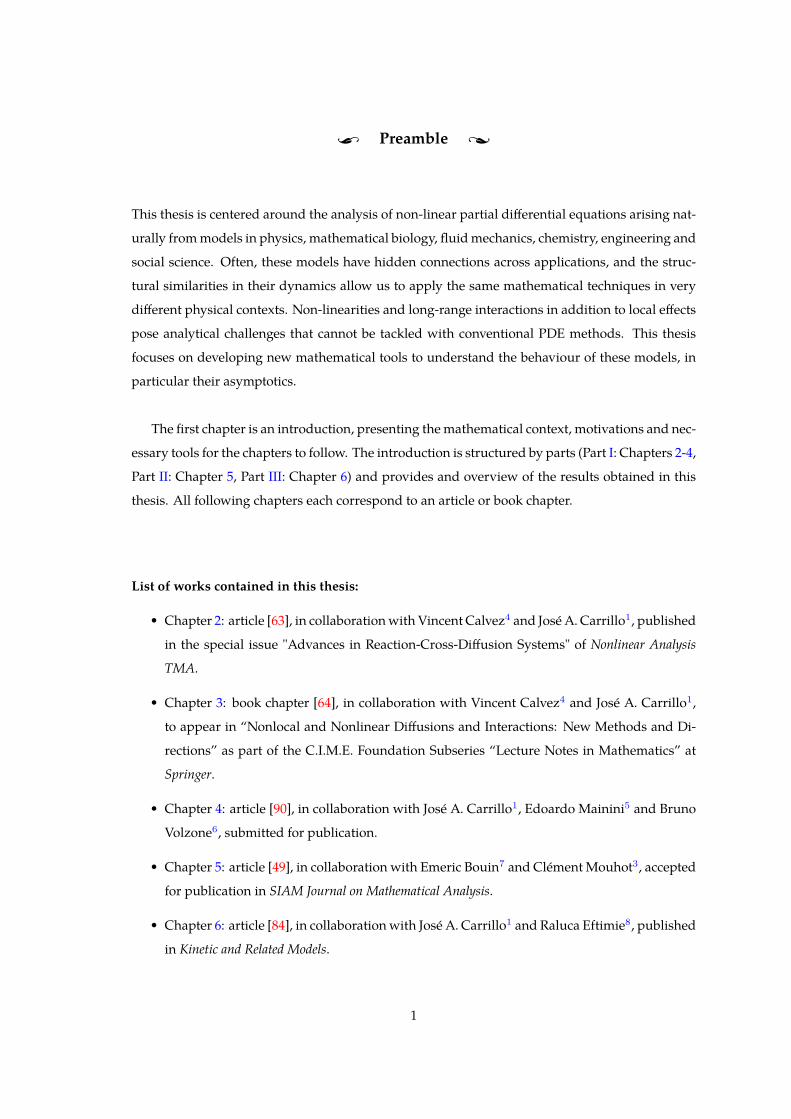
List of works contained in this thesis:
• Chapter 2: article [63], in collaborationwith Vincent Calvez4 and JoséA. Carrillo1, published
in the special issue "Advances in Reaction-Cross-Diffusion Systems" of Nonlinear Analysis
TMA.
• Chapter 3: book chapter [64], in collaboration with Vincent Calvez4 and José A. Carrillo1,
to appear in “Nonlocal and Nonlinear Diffusions and Interactions: New Methods and Di-
rections” as part of the C.I.M.E. Foundation Subseries “Lecture Notes in Mathematics” at
Springer.
• Chapter 4: article [90], in collaboration with José A. Carrillo1, Edoardo Mainini5 and Bruno
Volzone6, submitted for publication.
• Chapter 5: article [49], in collaboration with Emeric Bouin7 and Clément Mouhot3, accepted
for publication in SIAM Journal on Mathematical Analysis.
• Chapter 6: article [84], in collaborationwith José A. Carrillo1 and Raluca Eftimie8, published
in Kinetic and Related Models.
1
Contents
How to read this thesis
Each chapter is written to be self-contained. The logical relations between the chapters are the
following: Chapter 3 builds on the results in Chapter 2. Chapter 4 is tackling similar questions to
Chapter 2, but in a different regime, and using different tools in some cases. For part I, an overview
of the different regimes and their definitions can be found in Chapter 1. Chapters 5 and 6 are each
fully self-contained. The logical order of reading this thesis would be the order it is presented, or
changing the order of any of the parts I-III. A short overview of conclusions and perspectives can
be found at the very end of the thesis.
In order to keep the notation simple, equations are numbered by section number in each chap-
ter. For example, when reading Section 3 of Chapter 4, the first equation in that section would be
numbered (3.1). Cross-references to equations in other chapters are explicitly mentioned. When
reading Chapter 2, the same equation would be referenced as “equation (3.1) in Chapter 4”. The
same holds true for (sub)sections, theorems, definitions, propositions, corollaries, lemmata and
remarks. Figures however are numbered per chapter, e.g. Figure 3.14 refers to the 14th figure in
Chapter 3. References are listed together for all chapters at the end of the thesis in a general bibli-
ography.
All historical footnotes about mathematicians are taken either from [174], or from wikipedia10.
Funding
This thesis would not have been possible without the financial support that allowed its realisation.
It was supported by EPSRC grant number EP/H023348/1 (for the Cambridge Centre for Analy-
sis), ERCGrantMATKIT (ERC-2011-StG) and EPSRCGrantNumber EP/P031587/1, in addition to
funding fromanumber of organisations that supportedme in the attendance of conferences, work-
shops and research programs over the course of my Ph.D11. I would also like to thank Professor
Vincent Calvez, who generously supported numerous research visits to the ENS Lyon, resulting
in fruitful collaborations.
10www.wikipedia.org/.11Centro Internazionale Matematico Estivo (Italy), Christ’s College (Cambridge, UK), CNRS-PAN Mathematics Sum-
mer Institute (Cracow, Poland), Gran Sasso Science Institute (L’Aquila, Italy), Gruppo Nazionale per la Fisica Matemat-ica (Italy), Hausdorff Center for Mathematics (Bonn, Germany), Institute of Mathematics of Polish Academy of Sciences(Warsaw, Poland)), KI-Net ResearchNetwork inMathematical Sciences (US), Mittag-Leffler Institute (Stockholm, Sweden),Santander (UK).
2
Chapter1
Introduction
Chapter Content
1 The Keller–Segel model . . . . . . . . . . . . . . . . . . . . . . . . . . . . . . . . 8
2 Part I: Keller–Segel-type aggregation-diffusion equations . . . . . . . . . . . . . 10
2.1 Non-linear diffusion . . . . . . . . . . . . . . . . . . . . . . . . . . . . . . 11
2.2 Non-local interaction . . . . . . . . . . . . . . . . . . . . . . . . . . . . . 16
2.3 Attraction vs repulsion . . . . . . . . . . . . . . . . . . . . . . . . . . . . 19
3 Part I: Results . . . . . . . . . . . . . . . . . . . . . . . . . . . . . . . . . . . . . . 24
3.1 The different regimes . . . . . . . . . . . . . . . . . . . . . . . . . . . . . 24
3.2 Variations of HLS inequalities . . . . . . . . . . . . . . . . . . . . . . . . 27
3.3 The fair-competition regime . . . . . . . . . . . . . . . . . . . . . . . . . 32
3.4 The diffusion-dominated regime . . . . . . . . . . . . . . . . . . . . . . 39
4 Part I: Perspectives . . . . . . . . . . . . . . . . . . . . . . . . . . . . . . . . . . . 42
4.1 The fair-competition regimem “ mc . . . . . . . . . . . . . . . . . . . . 42
4.2 The diffusion-dominated regimem ą mc . . . . . . . . . . . . . . . . . 44
4.3 The aggregation-dominated regimem ă mc . . . . . . . . . . . . . . . . 44
5 Part II: Non-woven textiles . . . . . . . . . . . . . . . . . . . . . . . . . . . . . . . 46
5.1 Production process of non-woven textiles . . . . . . . . . . . . . . . . . 46
5.2 The fibre lay-down model . . . . . . . . . . . . . . . . . . . . . . . . . . 47
6 Part II: Hypocoercivity . . . . . . . . . . . . . . . . . . . . . . . . . . . . . . . . . 50
6.1 Abstract hypocoercivity approach: an example . . . . . . . . . . . . . . 51
6.2 Framework for linear kinetic equations . . . . . . . . . . . . . . . . . . . 53
7 Part II: Results . . . . . . . . . . . . . . . . . . . . . . . . . . . . . . . . . . . . . . 57
7.1 Functional framework . . . . . . . . . . . . . . . . . . . . . . . . . . . . . 58
7.2 Hypocoercivity estimate and convergence . . . . . . . . . . . . . . . . . 60
7.3 Perspectives . . . . . . . . . . . . . . . . . . . . . . . . . . . . . . . . . . 62
3
1. Introduction
8 Part III: From micro to macro . . . . . . . . . . . . . . . . . . . . . . . . . . . . . 64
8.1 The Boltzmann equation: grazing collisions . . . . . . . . . . . . . . . . 66
8.2 Bacterial chemotaxis: a kinetic description . . . . . . . . . . . . . . . . . 67
8.3 Parabolic scaling . . . . . . . . . . . . . . . . . . . . . . . . . . . . . . . . 68
9 Part III: Collective animal behaviour . . . . . . . . . . . . . . . . . . . . . . . . . 70
9.1 Overview of models and scalings . . . . . . . . . . . . . . . . . . . . . . 71
9.2 Asymptotic preserving numerical methods . . . . . . . . . . . . . . . . 75
9.3 Conclusions and perspectives . . . . . . . . . . . . . . . . . . . . . . . . 75
Most applied mathematicians spend their time developing, improving, analysing and testing
mathematical models – equations that describe a physical phenomenon – trying to make sense
of the (physical and/or mathematical) world. Of course, mathematical models will never be able
to capture the full reality and complexity of nature. Most of the models we currently use are
based on simplifying assumptions that are rarely satisfied in practice. This is not to say that sim-
plification renders a model less useful as a tool to understand the world. On the contrary, it is
this simplifying aspect that gives us powerful information about the dominant dynamics at play.
Good mathematical models find a reasonable trade-off between simplicity, complexity and math-
ematical difficulty. If a model is too simple, important physical features may be lost. If it is too
complex on the other hand, incorporating many details of the observed phenomena, we may not
be able to handle the analysis and so no useful information can be extracted from the model. It
is when we are able to successfully analyse a model that provides a reasonable approximation
to a complicated real world process that we can claim to have understood the dominant driving
principles – a powerful source of information for applications. In order to build the mathematical
tools and theories that allow us to handle the analysis of a particular equation, it is often useful to
start with amaster equation – the simplest model one can think of that is representative for a more
general class of models and still incorporates the common structural difficulties. One such master
equation for the class of models analysed in this thesis is the non-linear heat equation Btρ “ ∆ρm,
m ą 0 which appears in a number of applications across physics, chemistry, biology and engi-
neering (see Section 2.1 for more details). It extends the structural difficulty of another master
equation, the heat equation (m “ 1), by adding the non-linearity to the diffusion. Historically, it
has often been thanks to a representative master equation generating a rich mathematical theory
that more complex and therefore more realistic models could be tackled. What is so fascinating is
that models of similar mathematical form and difficulty can appear in the context of very differ-
ent applications. Understanding more about their general structure gives us new insights about
nature’s laws, allowing us to see the beautiful unifying patterns that surround us.
4
This thesis is centered around the analysis of non-linear partial differential equations arising
naturally from models in physics, mathematical biology, fluid mechanics, chemistry, engineer-
ing and social science. Often, these models have hidden connections across applications, and the
structural similarities in their dynamics allow us to apply the same mathematical techniques in
very different physical contexts. Non-linearities and long-range interactions in addition to local
effects pose analytical challenges that cannot be tackled with conventional PDE methods. This
thesis focuses on developing new mathematical tools to understand the behaviour of these mod-
els, in particular their asymptotics.
The choice of title for this thesis and the sense in which it is to be understood deserve a few
explanatory words. First of all, the term interacting particles should be taken in a very broad inter-
pretation. Here, the ’particles’ can represent for example molecules of a gas, single-cell organisms
such as bacteria, stars in a galaxy, lay-down points of polymer fibres, insects, fish, birds, ungulates,
or even humans. Correspondingly, the interaction of particles with each other, or with their envi-
ronment, could be via molecular forces, chemical signals1, gravitational forces, an external force
describing the coiling properties of the polymer fibres, or - in the case of animals and humans -
visual, auditory or tactile signals. The type of interaction could be linear or non-linear, local or
non-local. Both linear local interactions (Chapter 5) and non-linear non-local interactions (Chap-
ters 2, 3, 4 and 6) are considered in this thesis.
Secondly, let me comment on what I mean by asymptotic analysis. Two types of asymptotics
have to be distinguished:
(1) the behaviour of solutions predicted by the model after a very long time tÑ8which we call
long-time asymptotic behaviour or ergodic properties (Chapters 2-5), and
(2) the limiting equations obtained by letting certain parameters of a model be either very big or
very small (Chapter 6).
As suggested by the title, the main focus lies in the long-time asymptotic analysis, but we also
consider limiting processes.
In case (1), we want to know whether solutions converge to an asymptotic profile and if yes,
in which sense and how fast. What do these asymptotic profiles look like? How many are there,
and what is their basin of attraction? The natural candidates amongst which to look for asymp-
totic profiles are the equilibrium states of the model under consideration. This means that the first
1The ability of certain types of bacteria to respond to chemical gradients is known as bacterial chemotaxis, see Section 1.
5
1. Introduction
logical step towards understanding the asymptotic behaviour of solutions is often to study the sta-
tionary problem instead, which is our focus in Chapters 2, 3 and 4. It is only in Chapters 3 and 5
that we actually study the evolution problemwith the aim of finding explicit rates of convergence.
Case (2) makes the connection between different observation scales, using a set of methods
called multiscale analysis or scaling process or limiting process. Let us take the example of a mono-
atomic gas. Using Newton’s2 laws, one can write down an equation for n interacting gas particles
located at positions X1ptq, . . . , Xnptq. This type of model is usually referred to as a particle-based
model, or Individual Based Model (IBM) in the case where the particles represent living organisms,
see Section 2.2.2. In practice however, it is often hopeless to attempt to describe the position and
velocity of every particle if the number of particles is large3. Using statistical ideas, we can instead
describe the evolution of the probability density fpt, x, vq of a certain particle to be at location x
and travelling with velocity v at time t. One example of such a model is the Boltzmann equation
modelling the particle distribution of a monoatomic rarefied gas, see Section 8. This level of de-
scription is called kinetic since the function f depends not only on space and time, but also on
velocities. There are several techniques that allow us to go from a particle description to a kinetic
description of the same evolution process, but this interesting and still developing mathematical
field is not the focus of this thesis4. We may also want to make a connection between different
kinetic descriptions, for example when the difference between velocities before and after a colli-
sion is small, known as grazing collisions, see Section 8.1. In Chapter 6, we use this idea applied
to animals turning only a small angle upon interactions with neighbours such as migratory birds
following favourable winds or magnetic fields.
In practise however, all that our typical observation can detect are changes in the macroscopic
state of the gas, described by quantities such as density, bulk velocity, temperature, stresses, and
heat flow, and these are related to some suitable averages of quantities depending on the kinetic
probability density. It is therefore desirable to be able to describe the dynamics at a macroscopic
scale, using for example a hydrodynamic scaling5. The idea is to rescale time and space by the
change of variables pt, x, vq ÞÑ ptεγ , xε, vq for a small scaling parameter ε ! 1, together with
certain scaling assumptions specifying how the interaction term behaves in the limit ε Ñ 0. The
2Isaac Newton (1642-1727) was an English mathematician, astronomer, and physicist who is widely recognised as oneof the most influential scientists of all time and a key figure in the scientific revolution. His three laws of motion were firstpublished in PhilosophiæNaturalis Principia Mathematica in 1687. Beyond his work on the mathematical sciences, Newtondedicated much of his time to the study of alchemy and biblical chronology. In a manuscript from 1704 he estimated thatthe world would end no earlier than 2060.
3The number of air molecules at atmospheric pressure and at 0˝ C temperature is around 2.7 ˆ 1019 per cm3, a lotmore than what would be feasible to keep track of.
4Some of the more common regimes are low density limits, weak coupling limits ormean-field limits, see for example [259,263], or Section 2.2.4 for the latter.
5For more details on the techniques involved, see Sections 6.2.3 and 8.
6
two main scaling approaches are parabolic limits (γ “ 2) for which diffusive forces dominate, and
hyperbolic limits (γ “ 1), which are convective.
In terms of modelling perspective, Part I (Chapters 2-4) deals with a macroscopic model, Part
II (Chapter 5) is concernedwith a kinetic model, and Part III (Chapter 6) focuses on the connection
between different kinetic and macroscopic regimes using parabolic and grazing collision limits.
Finally, the term Keller–Segel-type models in the title of this thesis refers to models that are close
variations of what is known as the classical Keller–Segel model, which we describe in more detail
in the next section.
This introductory chapter is structured into 9 sections: Section 1 describes the classical Keller–
Segel model, and subsequent sections correspond to Part I (Sections 2-4), Part II (Sections 5-7) and
Part III (Sections 8-9) of this thesis. For each part, we explain the relevant mathematical tools,
introduce the models we are analysing in this thesis together with the most important notation,
give somemotivation and context of the problem, and last but not least, present a summary of the
results obtained and possible perspectives.
7
1. Introduction
1 The Keller–Segel model
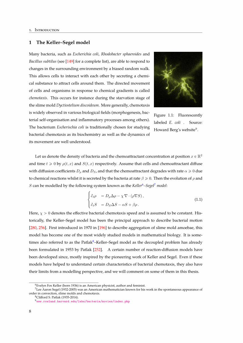
Figure 1.1: Fluorescently
labeled E. coli . Source:
Howard Berg’s website9.
Many bacteria, such as Escherichia coli, Rhodobacter sphaeroides and
Bacillus subtilus (see [149] for a complete list), are able to respond to
changes in the surrounding environment by a biased random walk.
This allows cells to interact with each other by secreting a chemi-
cal substance to attract cells around them. The directed movement
of cells and organisms in response to chemical gradients is called
chemotaxis. This occurs for instance during the starvation stage of
the slimemoldDyctiostelium discoideum. More generally, chemotaxis
is widely observed in various biological fields (morphogenesis, bac-
terial self-organisation and inflammatory processes among others).
The bacterium Escherischia coli is traditionally chosen for studying
bacterial chemotaxis as its biochemistry as well as the dynamics of
its movement are well understood.
Let us denote the density of bacteria and the chemoattractant concentration at position x P R2
and time t ě 0 by ρpt, xq and Spt, xq respectively. Assume that cells and chemoattractant diffuse
with diffusion coefficientsDρ andDS , and that the chemoattractant degrades with rate α ě 0 due
to chemical reactions whilst it is secreted by the bacteria at rate β ě 0. Then the evolution of ρ and
S can be modelled by the following system known as the Keller6–Segel7 model:$
’
&
’
%
Btρ “ Dρ∆ρ´ χ∇ ¨ pρ∇Sq ,
BtS “ DS∆S ´ αS ` βρ .(1.1)
Here, χ ą 0 denotes the effective bacterial chemotaxis speed and is assumed to be constant. His-
torically, the Keller–Segel model has been the principal approach to describe bacterial motion
[280, 256]. First introduced in 1970 in [196] to describe aggregation of slime mold amoebae, this
model has become one of the most widely studied models in mathematical biology. It is some-
times also referred to as the Patlak8–Keller–Segel model as the decoupled problem has already
been formulated in 1953 by Patlak [252]. A certain number of reaction-diffusion models have
been developed since, mostly inspired by the pioneering work of Keller and Segel. Even if these
models have helped to understand certain characteristics of bacterial chemotaxis, they also have
their limits from a modelling perspective, and we will comment on some of them in this thesis.
6Evelyn Fox Keller (born 1936) is an American physicist, author and feminist.7Lee Aaron Segel (1932-2005) was an American mathematician known for his work in the spontaneous appearance of
order in convection, slime molds and chemotaxis.8Clifford S. Patlak (1935-2014).9www.rowland.harvard.edu/labs/bacteria/movies/index.php
8
1. The Keller–Segel model
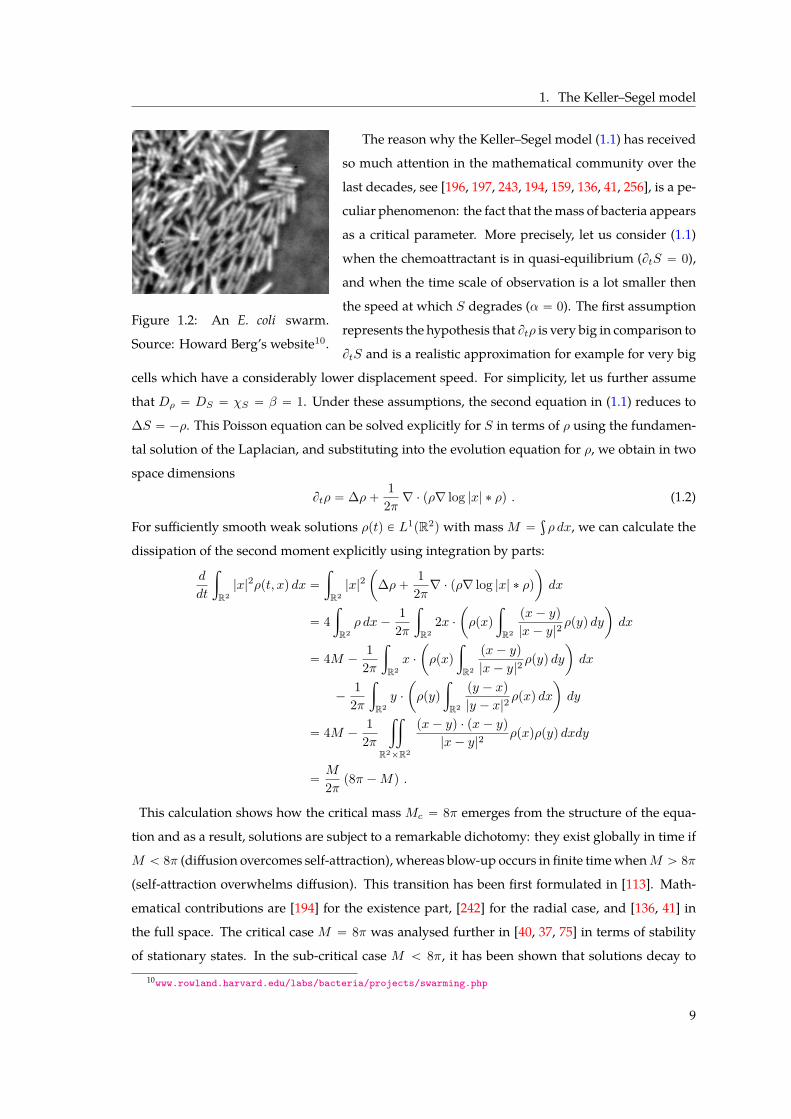
Figure 1.2: An E. coli swarm.
Source: Howard Berg’s website10.
The reason why the Keller–Segel model (1.1) has received
so much attention in the mathematical community over the
last decades, see [196, 197, 243, 194, 159, 136, 41, 256], is a pe-
culiar phenomenon: the fact that themass of bacteria appears
as a critical parameter. More precisely, let us consider (1.1)
when the chemoattractant is in quasi-equilibrium (BtS “ 0),
and when the time scale of observation is a lot smaller then
the speed at which S degrades (α “ 0). The first assumption
represents the hypothesis that Btρ is very big in comparison to
BtS and is a realistic approximation for example for very big
cells which have a considerably lower displacement speed. For simplicity, let us further assume
that Dρ “ DS “ χS “ β “ 1. Under these assumptions, the second equation in (1.1) reduces to
∆S “ ´ρ. This Poisson equation can be solved explicitly for S in terms of ρ using the fundamen-
tal solution of the Laplacian, and substituting into the evolution equation for ρ, we obtain in two
space dimensions
Btρ “ ∆ρ` 12π ∇ ¨ pρ∇ log |x| ˚ ρq . (1.2)
For sufficiently smooth weak solutions ρptq P L1pR2q with massM “ş
ρ dx, we can calculate the
dissipation of the second moment explicitly using integration by parts:
d
dt
ż
R2|x|2ρpt, xq dx “
ż
R2|x|2
ˆ
∆ρ` 12π∇ ¨ pρ∇ log |x| ˚ ρq
˙
dx
“ 4ż
R2ρ dx´
12π
ż
R22x ¨
ˆ
ρpxq
ż
R2
px´ yq
|x´ y|2ρpyq dy
˙
dx
“ 4M ´1
2π
ż
R2x ¨
ˆ
ρpxq
ż
R2
px´ yq
|x´ y|2ρpyq dy
˙
dx
´1
2π
ż
R2y ¨
ˆ
ρpyq
ż
R2
py ´ xq
|y ´ x|2ρpxq dx
˙
dy
“ 4M ´1
2π
ij
R2ˆR2
px´ yq ¨ px´ yq
|x´ y|2ρpxqρpyq dxdy
“M
2π p8π ´Mq .
This calculation shows how the critical massMc “ 8π emerges from the structure of the equa-
tion and as a result, solutions are subject to a remarkable dichotomy: they exist globally in time if
M ă 8π (diffusion overcomes self-attraction), whereas blow-up occurs in finite timewhenM ą 8π
(self-attraction overwhelms diffusion). This transition has been first formulated in [113]. Math-
ematical contributions are [194] for the existence part, [242] for the radial case, and [136, 41] in
the full space. The critical case M “ 8π was analysed further in [40, 37, 75] in terms of stability
of stationary states. In the sub-critical case M ă 8π, it has been shown that solutions decay to10www.rowland.harvard.edu/labs/bacteria/projects/swarming.php
9
1. Introduction
self-similarity solutions exponentially fast in suitable rescaled variables [70, 71, 148]. In the super-
critical caseM ą 8π, solutions blow-up in finite time with by now well studied blow-up profiles
for close enough to critical mass, see [187, 260, 168]. In part I of this thesis, we are generalising the
techniques developed in [62]where the authors show convergence to self-similarity inWasserstein
distance for (1.2) in the radial sub-critical caseM ă 8π.
2 Part I: Keller–Segel-type aggregation-diffusion equations
In the first andmain part of this thesis, we are studying the behaviour of a family of partial differen-
tial equations of Keller-Segel-type modelling self-attracting diffusive particles at the macroscopic
scale,
Btρ “1N
∆ρm ` 2χ∇ ¨ pρ∇pW ˚ ρqq , t ą 0 , x P RN . (2.3)
Here, the diffusion is non-linear if m ‰ 1, and the non-local interaction between particles is gov-
erned by the interaction potentialW withW : RN Ñ R,W P C1 `RNzt0u˘
andW p´xq “W pxq. The
parameter χ ą 0 is measuring the interaction strength of the interaction term in relation to the diffu-
sive term. Equation (2.3) exhibits three conservation laws: conservation of positivity, conservation
of mass, and invariance by translation. We can therefore assume for convenience
ρpt “ 0, xq “ ρ0pxq ě 0 ,ż
RNρ0pxq dx “ 1 ,
ż
RNxρ0pxq dx “ 0 . (2.4)
The parameter χ ą 0 scales with the mass of solutions ρ, and therefore, in the case where the
behaviour of solutions depends on the choice of initial mass, this criticality is transferred to the
parameter χ when fixing the mass. Let us point out that Part I does not address the questions of
regularity, existence, or uniqueness of solutions to equation (2.3), assuming solutions are ’nice’
enough in space and time for our analysis to hold.
We will now give some intuition to explain the type of behaviour that can be modelled using
equation (2.3). Conceptually, the PDE (2.3) corresponds to the assumption that two main forces
determine a particle’s motion at the microscopic level: local non-linear diffusion on the one hand,
and non-local attraction on the other hand. Diffusion can be understood as a repulsive force be-
tween particles, whereas the interaction between particles is assumed to be represented by an
attractive potential, W . Here, attractive and repulsive forces compete, generating complex be-
hviour of solutions, depending on the diffusion power m, the choice of interaction potential W ,
the interaction strength χ ą 0 and the dimensionality N .
The reason why models of the form (2.3) have attracted so much attention in recent years is not
only their richmathematical structure, but also their applicability to awide range of physical prob-
lems ranging from collective behaviour of self-interacting individuals such as bacterial chemo-
10
2. Part I: Keller–Segel-type aggregation-diffusion equations
taxis [39, 196, 252], astrophysics [108, 271, 105, 107, 106] and mean-field games [38] to phase tran-
sitions [285] and opinion dynamics [164, 165].
Before diving into the analysis of (2.3), let us investigate the dynamics of attractive and repul-
sive forces separately.
2.1 Non-linear diffusion
Assuming χ “ 0, one can interpret equation (2.3) as a non-linear heat equation, where the diffu-
sion coefficient varies with the density of particles,
Btρ “1N
∆ρm “ ∇ ¨ pDpρq∇ρq , Dpρq :“ m
Nρm´1 , m ą 0 . (2.5)
As above, we assume that the initial data satisfies (2.4). Diffusion can be understood as a repulsive
force since ’nice’ enough solutions ρ of (2.5) satisfy
d
dt
ż
RN|x|2ρpt, xq dx “ 2
ż
RNρmpt, xq dx .
It follows that if ρpt, ¨q P L1`pRN q X LmpRN q for any t ą 0, then the second moment of ρ increases
with time, that is, the solution is spreading out. The resulting effect is that particles get repulsed
away from each other.
Equation (2.5) is one of the simplest examples of a non-linear evolution equation of parabolic
type. It appears in a natural way in a number of applications across physics, chemistry, biology
and engineering. The common idea is that in many diffusion processes the diffusion coefficient
depends on the unknown quantities (concentration, density, temperature, etc.) of the diffusion
model.
For any diffusion exponentm ą 0, a unique mild solution exists for any initial data ρ0 P L1pRN q,
it depends continuously on the initial data, and further, the concepts of mild, weak and strong
solution are equivalent [287, 25, 286]. Thanks to the form of the diffusion coefficient Dpρq, the
overall behaviour of solutions can be split into three cases:
• m ą 1: Diffusion is slow in areas with few particles. This case is known as the porous
medium equation (PME), or slow diffusion equation. The PME owes its name to the mod-
eling of the flow of an isentropic gas through a porous medium [216, 241]. It was introduced
for the study of groundwater infiltration [51], and is used in high-temperature physics, e.g.
in the context of heat radiation in plasmas [303]. Other applications have been proposed in
mathematical biology, spread of viscous fluids, boundary layer theory, see [289, 287, 7, 286,
161] and the references therein.
11
1. Introduction
• m “ 1: Diffusion is linear, and we obtain the well-known heat equation (HE) [156].
• 0 ă m ă 1: Diffusion is fast in areas with few particles. This case is known as the fast
diffusion equation (FDE). The FDE appears in plasma physics (m “ 12 is known as the
Okuda-Dawson law [246]), and when modelling the diffusion of impurities in silicon [200].
The FDE has also an important application in geometry known as the Yamabe flow (m “
pN ´ 2qpN ` 2q, N ě 3) [215, 288].
Note that problems may arise when diffusion is ’too fast’, i.e. when the diffusion coefficient
m is very small. It is established in [186] that the range of mass conservation for the FDE is
m˚ ă m ă 1 with
m˚ ă m ă 1 , m˚ :“
$
’
&
’
%
0 , ifN “ 1, 2 ,
1´ 2N , ifN ě 3 .
This is exactly the range for which integrable solutions to (2.5) exist. Within this range,
the flow associated to the fast diffusion equation is in many ways even better than the flow
associated to the heat equation; see [48] and the references therein. If m˚ ă m ă 1, the
solutions of (2.5) with positive integrable initial data are C8 and strictly positive everywhere
instantaneously, just as for the heat flow.
Equation (2.5) gives rise to a rich mathematical theory with fundamental differences in behaviour
depending on these three different regimes for the diffusion exponent m ą 0. We will see later
that some of these behaviour carry over to our aggregation-diffusion equation (2.3). This illus-
trates how the non-linear heat equation serves as an important representative for a more general
class of non-linear, formally parabolic equations that appear across the pure and applied sciences,
and it has been at the heart of the development of new analytical tools that can be adapted to a
range of more complicatedmodels. Wewill therefore give a short overview of themain properties
of the non-linear heat equation (2.5) that are relevant in the context of this thesis. For a more de-
tailed study dealing with the problems of existence, uniqueness, stability, regularity, dynamical
properties and asymptotic behaviour, we refer the reader to [289] (m ą 1), [300] (m “ 1), [287]
(0 ă m ă 1), and the references therein.
2.1.1 Source solutions
A classical problem in the thermal propagation theory is to describe the evolution of a heat dis-
tribution after a point source release. In mathematical terms, we want to find a solution Φmpt, xq
to (2.5) with initial data given by a Dirac Delta, ρ0pxq “ δpxq. In case of the heat equation (m “ 1),
this fundamental solution is well-known and is given by the heat kernel
Φ1pt, xq “ p4πtq´N2 exp
ˆ
´|x|2
4t
˙
.
12
2. Part I: Keller–Segel-type aggregation-diffusion equations
It is especially useful to have source solutions given in explicit form, as they often serve as a repre-
sentative example for the typical or peculiar behaviour of solutions. Further, for linear equations,
they allow us to obtain the general solution by applying a convolution, ρ “ Φ1 ˚ ρ0. Such an ap-
proach is useless in the non-linear setting, and so one needs different methods. In case of the PME
(m ą 1), source solutions are given by
Φmpt, xq “ t´αFm
´
xt´αN¯
, Fmpξq :“`
β`
|ξ0|2 ´ |ξ|2
˘˘1
m´1`
, m ą 1 , (2.6)
for any ξ0 P RN , ξ0 ‰ 0, where we define the positive part as psq` :“ maxts, 0u and where
α :“ N
Npm´ 1q ` 2 , β :“ αpm´ 1q2Nm . (2.7)
SolutionsΦm depend continuously onm and converge pointwise to the heat kernel asmÑ 1. This
class of special solutions was first obtained by Zel’dovich and Kompaneets [304] around 1950, and
then studied inmore detail by Barenblatt [14] andPattle [253]. They arewidely known asBarenblatt
solutions (or, for a more complete reference, as ZKB solutions or Barenblatt-Pattle solutions). For
more details on (2.6) and their derivation, see [289] and the references therein.
In fact, the same source solution (2.6) also exists for the FDE in the regimem ă 1 as long as α ą 0,
that is,m ą m˚. The solution Φm is then given by the same type of expression,
Φmpt, xq “ t´αGm
´
xt´αN¯
, Gmpξq :“`
C ` β|ξ|2˘´ 1
1´m , m˚ ă m ă 1 , (2.8)
where β :“ ´β “ αp1´mqp2Nmq, and C “ CpN,mq ą 0 is a normalising constant fixed by the
mass. Therefore, we obtain for the source solution of the FDE form˚ ă m ă 1:
Φmpt, xq1´m “t
Ct2αN ` β|x|2.
In this sense, the Barenblatt self-similar solutions for m ‰ 1, m ą m˚ are natural generalisations
of the fundamental solutions of the heat equation.
2.1.2 Support and Tails
The main difference between the source-type solution profiles in the different ranges is probably
the shape at infinity, which reflects the propagation form. If m ą 1, the profile Fm is compactly
supported, supp pFmq “ Bp0, |ξ0|q, and it follows that the Barenblatt solution Φm has compact
support in space for every fixed time t ą 0. More precisely, the free boundary is the surface given
by the equation
t “
ˆ
|x|
|ξ0|
˙Npm´1q`2,
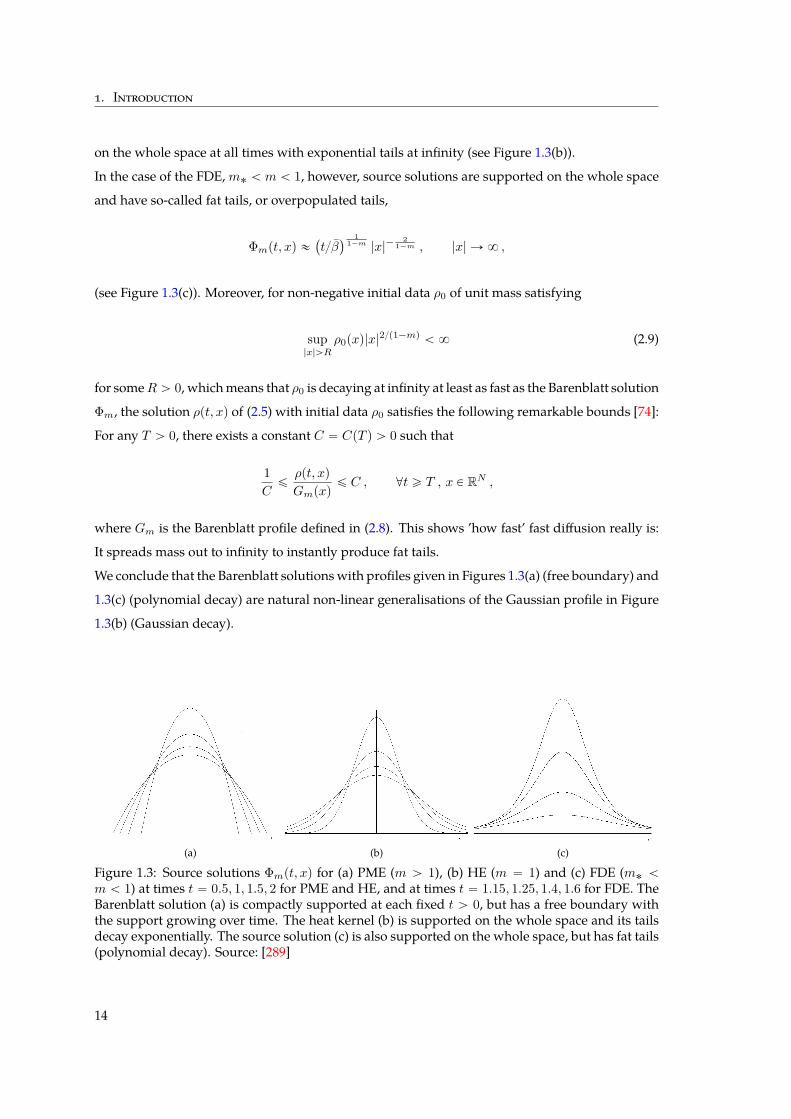
and so the size of the support supp pΦmq growswith a precise finite speed (see Figure 1.3(a)). This
is to be compared with the properties of the heat kernel Φ1 in the casem “ 1, which is supported
13
1. Introduction
on the whole space at all times with exponential tails at infinity (see Figure 1.3(b)).
In the case of the FDE,m˚ ă m ă 1, however, source solutions are supported on the whole space
and have so-called fat tails, or overpopulated tails,
Φmpt, xq «`
tβ˘
11´m |x|´
21´m , |x| Ñ 8 ,
(see Figure 1.3(c)). Moreover, for non-negative initial data ρ0 of unit mass satisfying
sup|x|ąR
ρ0pxq|x|2p1´mq ă 8 (2.9)
for someR ą 0, whichmeans that ρ0 is decaying at infinity at least as fast as the Barenblatt solution
Φm, the solution ρpt, xq of (2.5) with initial data ρ0 satisfies the following remarkable bounds [74]:
For any T ą 0, there exists a constant C “ CpT q ą 0 such that
1Cďρpt, xq
Gmpxqď C , @t ě T , x P RN ,
where Gm is the Barenblatt profile defined in (2.8). This shows ’how fast’ fast diffusion really is:
It spreads mass out to infinity to instantly produce fat tails.
We conclude that the Barenblatt solutionswith profiles given in Figures 1.3(a) (free boundary) and
1.3(c) (polynomial decay) are natural non-linear generalisations of the Gaussian profile in Figure
1.3(b) (Gaussian decay).
(a) (b) (c)
Figure 1.3: Source solutions Φmpt, xq for (a) PME (m ą 1), (b) HE (m “ 1) and (c) FDE (m˚ ăm ă 1) at times t “ 0.5, 1, 1.5, 2 for PME and HE, and at times t “ 1.15, 1.25, 1.4, 1.6 for FDE. TheBarenblatt solution (a) is compactly supported at each fixed t ą 0, but has a free boundary withthe support growing over time. The heat kernel (b) is supported on the whole space and its tailsdecay exponentially. The source solution (c) is also supported on the whole space, but has fat tails(polynomial decay). Source: [289]
14
2. Part I: Keller–Segel-type aggregation-diffusion equations
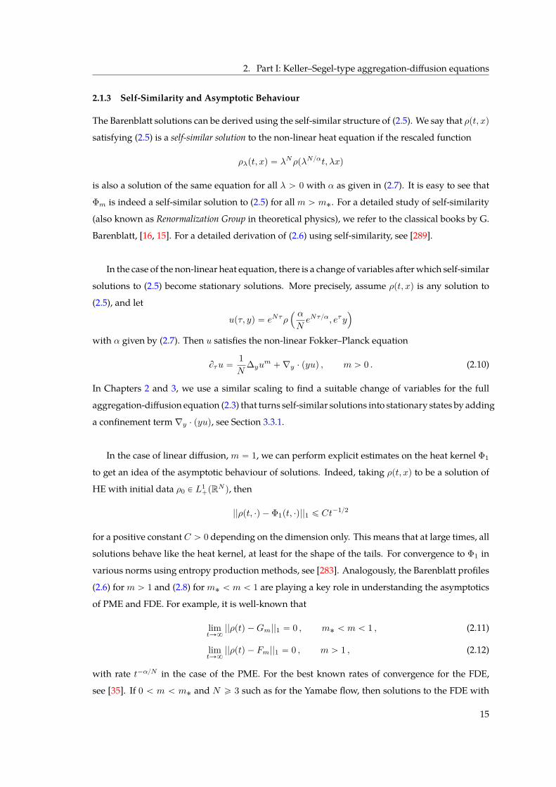
2.1.3 Self-Similarity and Asymptotic Behaviour
The Barenblatt solutions can be derived using the self-similar structure of (2.5). We say that ρpt, xq
satisfying (2.5) is a self-similar solution to the non-linear heat equation if the rescaled function
ρλpt, xq “ λNρpλNαt, λxq
is also a solution of the same equation for all λ ą 0 with α as given in (2.7). It is easy to see that
Φm is indeed a self-similar solution to (2.5) for allm ą m˚. For a detailed study of self-similarity
(also known as Renormalization Group in theoretical physics), we refer to the classical books by G.
Barenblatt, [16, 15]. For a detailed derivation of (2.6) using self-similarity, see [289].
In the case of the non-linear heat equation, there is a change of variables afterwhich self-similar
solutions to (2.5) become stationary solutions. More precisely, assume ρpt, xq is any solution to
(2.5), and let
upτ, yq “ eNτρ´ α
NeNτα, eτy
¯
with α given by (2.7). Then u satisfies the non-linear Fokker–Planck equation
Bτu “1N
∆yum `∇y ¨ pyuq , m ą 0 . (2.10)
In Chapters 2 and 3, we use a similar scaling to find a suitable change of variables for the full
aggregation-diffusion equation (2.3) that turns self-similar solutions into stationary states by adding
a confinement term ∇y ¨ pyuq, see Section 3.3.1.
In the case of linear diffusion,m “ 1, we can perform explicit estimates on the heat kernel Φ1
to get an idea of the asymptotic behaviour of solutions. Indeed, taking ρpt, xq to be a solution of
HE with initial data ρ0 P L1`pRN q, then
||ρpt, ¨q ´ Φ1pt, ¨q||1 ď Ct´12
for a positive constant C ą 0 depending on the dimension only. This means that at large times, all
solutions behave like the heat kernel, at least for the shape of the tails. For convergence to Φ1 in
various norms using entropy production methods, see [283]. Analogously, the Barenblatt profiles
(2.6) form ą 1 and (2.8) form˚ ă m ă 1 are playing a key role in understanding the asymptotics
of PME and FDE. For example, it is well-known that
limtÑ8
||ρptq ´Gm||1 “ 0 , m˚ ă m ă 1 , (2.11)
limtÑ8
||ρptq ´ Fm||1 “ 0 , m ą 1 , (2.12)
with rate t´αN in the case of the PME. For the best known rates of convergence for the FDE,
see [35]. If 0 ă m ă m˚ and N ě 3 such as for the Yamabe flow, then solutions to the FDE with
15
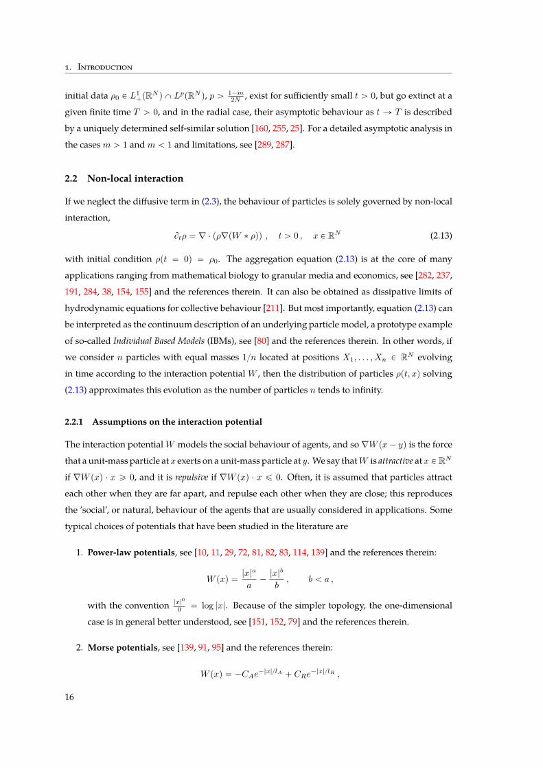
1. Introduction
initial data ρ0 P L1`pRN q X LppRN q, p ą 1´m
2N , exist for sufficiently small t ą 0, but go extinct at a
given finite time T ą 0, and in the radial case, their asymptotic behaviour as t Ñ T is described
by a uniquely determined self-similar solution [160, 255, 25]. For a detailed asymptotic analysis in
the casesm ą 1 andm ă 1 and limitations, see [289, 287].
2.2 Non-local interaction
If we neglect the diffusive term in (2.3), the behaviour of particles is solely governed by non-local
interaction,
Btρ “ ∇ ¨ pρ∇pW ˚ ρqq , t ą 0 , x P RN (2.13)
with initial condition ρpt “ 0q “ ρ0. The aggregation equation (2.13) is at the core of many
applications ranging from mathematical biology to granular media and economics, see [282, 237,
191, 284, 38, 154, 155] and the references therein. It can also be obtained as dissipative limits of
hydrodynamic equations for collective behaviour [211]. But most importantly, equation (2.13) can
be interpreted as the continuum description of an underlying particle model, a prototype example
of so-called Individual Based Models (IBMs), see [80] and the references therein. In other words, if
we consider n particles with equal masses 1n located at positions X1, . . . , Xn P RN evolving
in time according to the interaction potential W , then the distribution of particles ρpt, xq solving
(2.13) approximates this evolution as the number of particles n tends to infinity.
2.2.1 Assumptions on the interaction potential
The interaction potentialW models the social behaviour of agents, and so ∇W px´ yq is the force
that a unit-mass particle at x exerts on a unit-mass particle at y. We say thatW is attractive atx P RN
if ∇W pxq ¨ x ě 0, and it is repulsive if ∇W pxq ¨ x ď 0. Often, it is assumed that particles attract
each other when they are far apart, and repulse each other when they are close; this reproduces
the ’social’, or natural, behaviour of the agents that are usually considered in applications. Some
typical choices of potentials that have been studied in the literature are
1. Power-law potentials, see [10, 11, 29, 72, 81, 82, 83, 114, 139] and the references therein:
W pxq “|x|a
a´|x|b
b, b ă a ,
with the convention |x|0
0 “ log |x|. Because of the simpler topology, the one-dimensional
case is in general better understood, see [151, 152, 79] and the references therein.
2. Morse potentials, see [139, 91, 95] and the references therein:
W pxq “ ´CAe´|x|lA ` CRe
´|x|lR ,
16
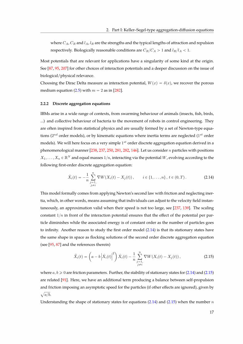
2. Part I: Keller–Segel-type aggregation-diffusion equations
whereCA,CR and lA, lR are the strengths and the typical lengths of attraction and repulsion
respectively. Biologically reasonable conditions are CRCA ą 1 and lRlA ă 1.
Most potentials that are relevant for applications have a singularity of some kind at the origin.
See [87, 95, 207] for other choices of interaction potentials and a deeper discussion on the issue of
biological/physical relevance.
Choosing the Dirac Delta measure as interaction potential, W pxq “ δpxq, we recover the porous
medium equation (2.5) withm “ 2 as in [282].
2.2.2 Discrete aggregation equations
IBMs arise in a wide range of contexts, from swarming behaviour of animals (insects, fish, birds,
...) and collective behaviour of bacteria to the movement of robots in control engineering. They
are often inspired from statistical physics and are usually formed by a set of Newton-type equa-
tions (2nd order models), or by kinematic equations where inertia terms are neglected (1st order
models). We will here focus on a very simple 1st order discrete aggregation equation derived in a
phenomenological manner [238, 237, 250, 281, 282, 146]. Let us consider n particles with positions
X1, . . . , Xn P RN and equal masses 1n, interacting via the potentialW , evolving according to the
following first-order discrete aggregation equation:
9Xiptq “ ´1n
nÿ
j“1,j‰i
∇W pXiptq ´Xjptqq , i P t1, . . . , nu , t P p0, T q . (2.14)
This model formally comes from applying Newton’s second lawwith friction and neglecting iner-
tia, which, in other words, means assuming that individuals can adjust to the velocity field instan-
taneously, an approximation valid when their speed is not too large, see [237, 139]. The scaling
constant 1n in front of the interaction potential ensures that the effect of the potential per par-
ticle diminishes while the associated energy is of constant order as the number of particles goes
to infinity. Another reason to study the first order model (2.14) is that its stationary states have
the same shape in space as flocking solutions of the second order discrete aggregation equation
(see [95, 87] and the references therein)
:Xiptq “
ˆ
a´ bˇ
ˇ
ˇ
9Xiptqˇ
ˇ
ˇ
2˙
9Xiptq ´1n
nÿ
j“1,j‰i
∇W pXiptq ´Xjptqq , (2.15)
where a, b ě 0 are friction parameters. Further, the stability of stationary states for (2.14) and (2.15)
are related [91]. Here, we have an additional term producing a balance between self-propulsion
and friction imposing an asymptotic speed for the particles (if other effects are ignored), given bya
ab.
Understanding the shape of stationary states for equations (2.14) and (2.15) when the number n
17
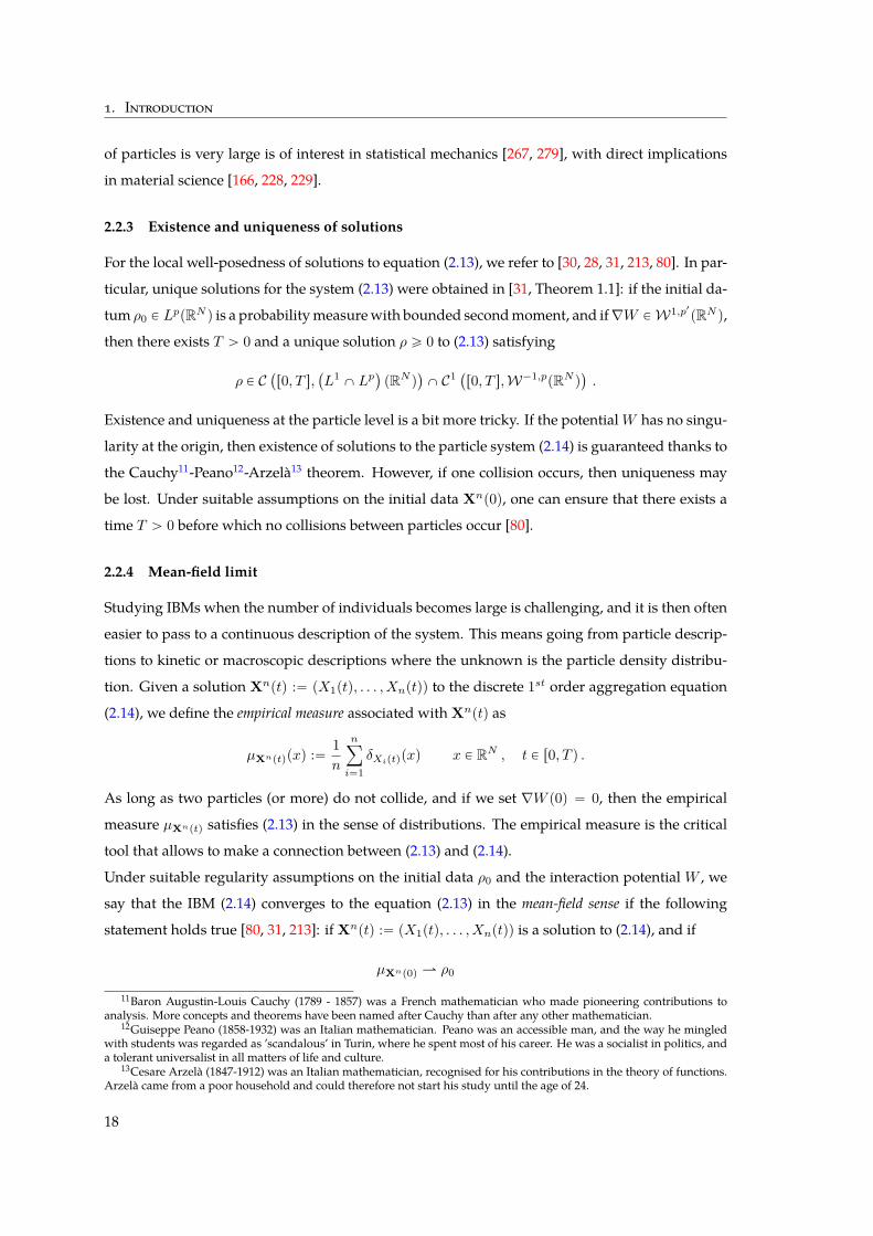
1. Introduction
of particles is very large is of interest in statistical mechanics [267, 279], with direct implications
in material science [166, 228, 229].
2.2.3 Existence and uniqueness of solutions
For the local well-posedness of solutions to equation (2.13), we refer to [30, 28, 31, 213, 80]. In par-
ticular, unique solutions for the system (2.13) were obtained in [31, Theorem 1.1]: if the initial da-
tum ρ0 P LppRN q is a probabilitymeasurewith bounded secondmoment, and if∇W P W1,p1pRN q,
then there exists T ą 0 and a unique solution ρ ě 0 to (2.13) satisfying
ρ P C`
r0, T s,`
L1 X Lp˘
pRN q˘
X C1 `r0, T s,W´1,ppRN q˘
.
Existence and uniqueness at the particle level is a bit more tricky. If the potentialW has no singu-
larity at the origin, then existence of solutions to the particle system (2.14) is guaranteed thanks to
the Cauchy11-Peano12-Arzelà13 theorem. However, if one collision occurs, then uniqueness may
be lost. Under suitable assumptions on the initial data Xnp0q, one can ensure that there exists a
time T ą 0 before which no collisions between particles occur [80].
2.2.4 Mean-field limit
Studying IBMs when the number of individuals becomes large is challenging, and it is then often
easier to pass to a continuous description of the system. This means going from particle descrip-
tions to kinetic or macroscopic descriptions where the unknown is the particle density distribu-
tion. Given a solution Xnptq :“ pX1ptq, . . . , Xnptqq to the discrete 1st order aggregation equation
(2.14), we define the empirical measure associated with Xnptq as
µXnptqpxq :“ 1n
nÿ
i“1δXiptqpxq x P RN , t P r0, T q .
As long as two particles (or more) do not collide, and if we set ∇W p0q “ 0, then the empirical
measure µXnptq satisfies (2.13) in the sense of distributions. The empirical measure is the critical
tool that allows to make a connection between (2.13) and (2.14).
Under suitable regularity assumptions on the initial data ρ0 and the interaction potential W , we
say that the IBM (2.14) converges to the equation (2.13) in the mean-field sense if the following
statement holds true [80, 31, 213]: if Xnptq :“ pX1ptq, . . . , Xnptqq is a solution to (2.14), and if
µXnp0q á ρ0
11Baron Augustin-Louis Cauchy (1789 - 1857) was a French mathematician who made pioneering contributions toanalysis. More concepts and theorems have been named after Cauchy than after any other mathematician.
12Guiseppe Peano (1858-1932) was an Italian mathematician. Peano was an accessible man, and the way he mingledwith students was regarded as ’scandalous’ in Turin, where he spent most of his career. He was a socialist in politics, anda tolerant universalist in all matters of life and culture.
13Cesare Arzelà (1847-1912) was an Italian mathematician, recognised for his contributions in the theory of functions.Arzelà came from a poor household and could therefore not start his study until the age of 24.
18
2. Part I: Keller–Segel-type aggregation-diffusion equations
in the weak-˚ sense as nÑ8, then
µXnptq á ρptq , @t P r0, T q ,
where ρptq is a solution to (2.13) with initial data ρpt “ 0q “ ρ0. We will not go into the details of
the rigorous proof for this statement, but the fact that equation (2.13) is the good choice of model
to represent the many-particle limit of (2.14) can also be understood on a more intuitive level as
follows: Assume that, instead of a finite number of particles, wewant tomodel the particle density
ρpx, tq. Then, according to (2.14), particles located at x at time tmove with velocity
vpt, xq “ ´
ż
RN∇W px´ yq ρpt, yqdy “ ´∇W ˚ ρ .
This leads to the conservation law Btρ`∇ ¨ pρvq “ 0, which is (2.13).
The regularity of the interaction potentialW is key for the type of convergence result that can
be obtained when going from (2.14) to (2.13). The classical Dobrushin strategy [131] for mean-
field limits applies to (2.13) only for C2pRN q smooth potentialsW with at most quadratic growth
at infinity [170]. In [80], the authors extended this result to more singular potentials.
In practise, one is interested in finding particle approximations Xnp0q to probability distribu-
tions ρ0 such that the corresponding empirical measure converges to that distribution in a desired
topology and satisfies certain constraints. This is an interesting and challenging mathematical
problem that has received a lot of attention in recent years, see for example [235, 50, 204, 176] and
the references therein.
2.3 Attraction vs repulsion
If the repulsion strength is very large at the origin, one can model repulsive effects by (non-linear)
diffusion while attraction is considered via non-local long-range forces [240, 282]. The main goal
of Part I is to understand better the behaviour of solutions when both non-linear diffusion and
non-local interactions are at play. The natural question that arises when combining aggregation
and diffusion terms is: which of the two forces wins, attraction or repulsion, and in which math-
ematical sense?
We will investigate this interplay for equation (2.3) with a rather simple yet challenging choice of
potential giving rise to a rich set of behaviour patterns:
Wkpxq “
$
’
&
’
%
|x|k
k, if k P p´N,Nqzt0u
log |x| , if k “ 0. (2.16)
19
1. Introduction
The conditions on k imply that the kernel Wk is locally integrable in RN . We need to make sure
that the aggregation term in (2.3) makes sense with this choice of potential. Let us define the
mean-field potential by Skpxq :“ Wkpxq ˚ ρpxq. For k ą 1´N , the gradient ∇Sk :“ ∇ pWk ˚ ρq is
well defined. For ´N ă k ď 1´N however, it becomes a singular integral, and we thus define it
via a Cauchy principal value,
∇Skpxq “ limεÑ0
ż
Bcpx,εq
|x´ y|k´2px´ yqρpyq dy
“
ż
RN|x´ y|k´2px´ yq pρpyq ´ ρpxqq dy ,
where Bcpx, εq :“ RNzBpx, εq is the complement of the ball of radius ε ą 0 centered at x P RN .
Hence, the mean-field potential gradient in equation (2.3) is given by
∇Skpxq :“
$
’
’
&
’
’
%
∇Wk ˚ ρ , if k ą 1´N ,
ż
RN∇Wkpx´ yq pρpyq ´ ρpxqq dy , if ´N ă k ď 1´N .
(2.17)
For k P p´N, 0q,Wk is also known as the Riesz14 potential, and writing k “ 2s´N with s P`
0, N2˘
,
the convolution term Sk is governed by a fractional diffusion process,
cN,sp´∆qsSk “ ρ , cN,s “ p2s´NqΓ`
N2 ´ 2s
˘
πN24sΓpsq“
kΓ`
´k ´ N2˘
πN22k`NΓ`
k`N2
˘ .
In terms of regularity, this means that Sk P W2s,ploc pRN q if ρ P L1pRN q X LppRN q, 1 ă p ă 8.
2.3.1 Energy functional and convexity properties
We make use of the special structure of equation (2.3), and its connection to the following free
energy functional:
Fm,krρs “ż
RNUm pρpxqq dx` χ
ij
RNˆRN
Wkpx´ yqρpxqρpyq dxdy (2.18)
with
Umpρq “
$
’
’
&
’
’
%
1Npm´ 1qρ
m , if m ‰ 1
1Nρ log ρ , if m “ 1
.
To simplify notation, we sometimes write
Fm,krρs :“ Umrρs ` χWkrρs ,
denoting by Um and Wk the repulsive and attractive contributions respectively. For Fm,k to be
finite, we require ρ P L1pRN q X LmpRN q, and additionally |x|kρ P L1pRN q in the case k ą 0. Note
14Frigyes (Frédéric) Riesz (1880-1956) was a Hungarian mathematician who made fundamental contributions to func-tional analysis. He had an uncommonmethod of giving lectures: a docent reading passages fromRiesz’s handbook and anassistant inscribing the appropriate equations on the blackboard, while Riesz himself stood aside, nodding occasionally.
20
2. Part I: Keller–Segel-type aggregation-diffusion equations
thatFm,k is invariant by translation, andwe assume as for the aggregation-diffusion equation (2.3)
that ρ ě 0,ş
ρ dx “ 1 andş
xρ dx “ 0.
One of themain goals in Part I is making the connection betweenminimisers of the free energy
functional (2.18) and stationary states of equation (2.3). Thanks to this connection, it is possible to
show existence and uniqueness of stationary states to (2.3) by studying the existence and unique-
ness of minimisers to the free energy functional Fm,k. This is where the notion of convexity be-
comes important. In simple terms, if a real valued function f : RN Ñ R is strictly convex, then
existence of a minimiser for f implies that it must be unique. McCann [234] discovered that there
is a similar underlying convexity structure for functionals defined on absolutely continuous Borel
measures, E : PacpRN q Ñ R, using an interpolation between Borel measures following the line of
optimal transportation [295]. Moreover, he used the powerful toolbox of Euclidean optimal trans-
portation to analyse functionals like (2.18) in the case m ě 0 and for a convex interaction kernel
Wk. Here, we deal with concave homogeneous interaction kernels Wk given by (2.16) for which
McCann’s results [234] do not apply.
We begin by introducing some tools from optimal transport. Let ρ and ρ be two probability
densities. According to [53, 233], there exists a convex function ψ whose gradient pushes forward
the measure ρpaqda onto ρpxqdx: ∇ψ# pρpaqdaq “ ρpxqdx. In other words, for any test function
ϕ P CbpRN q, the following identity holds trueż
RNϕp∇ψpaqqρpaq da “
ż
RNϕpxqρpxq dx .
The convex map ϕ is known as Brenier’s map , it is unique a.e. with respect to ρ and gives a way
of interpolating measures. The interpolating curve ρs, s P r0, 1s, with ρ0 “ ρ and ρ1 “ ρ can be
defined as ρspxq dx “ ps∇ψ`p1´sqIdN qpxq#ρpxq dxwhere IdN stands for the identity map inRN .
In fact, this interpolating curve is the minimal geodesic joining the measures ρpxqdx and ρpxqdx.
The notion of convexity associated to these interpolating curves is nothing else than convexity
along geodesics, introduced and called displacement convexity in [234]. Let us denote by PacpRN q
the set of absolutely continuous probability measures on RN .
Definition 2.1 (Displacement convexity). A functional E : PacpRN q Ñ R is (strictly) displacement
convex if
s ÞÑ E rpp1´ sqIdN ` s∇ψq#µs
is (strictly) convex on r0, 1s for any µ, ν P Pac, and where ψ is the corresponding Brenier map ν “ ∇ψ#µ.
The reason why we are interested in the displacement convexity properties of Fm,k is the fol-
lowing key result from [234]:
21
1. Introduction
Theorem 2.2 (McCann, 1997). If E : PacpRN q Ñ R is strictly displacement convex, then it has at most
one minimiser up to translation.
In other words, one recovers the property that existence of a minimiser implies uniqueness. In
our case however, Fm,k is not necessarily displacement convex. The convexity of the functionals
Um and Wk can be summarised as follows [234, 85, 98]:
Theorem 2.3. The functional Umrρs is displacement-convex provided thatm ě 1´ 1N . The functional
Wkrρs in one dimension is displacement-concave if k P p´1, 1q and displacement-convex for k ě 1 in any
dimension.
Therefore, the overall displacement-concavity/convexity of the energy functional Fm,k is not
known since:
• ifN “ 1, then Umrρs is displacement-convex for anym ě 0 and Wkrρs displacement-concave
since k P p´1, 1q;
• if N ą 1 and k P p1, Nq, then Wkrρs is displacement-convex, but we have no information
about the displacement-convexity of Umrρs;
• ifN ą 1 and k P p´N, 1q, then we have no information about the displacement-convexity of
Wkrρs.
We already observe that at least in one dimension we are dealing with the compensation between
the displacement-convexity of the internal energy Umrρs and the displacement-concavity of the
interaction energy Wkrρs. In Chapter 3, we will show that in certain cases, existence of a critical
point for Fm,k implies its uniqueness (up to translations and dilations) in the one dimensional
setting. Our main statement is that the functional (2.18) – the sum of a convex and a concave
functional – behaves almost like a convex functional when attractive and repulsive forces are in
balance. The bad functional contribution is somehow absorbed by the convex part for certain
homogeneity relations and parameters χ.
2.3.2 Gradient flow structure
The strong connection between the functional Fm,k and the PDE (2.3) is due to the fact that the
functional Fm,k is non-increasing along the trajectories of the system as it satisfies at least formally
d
dtFm,krρptqs “ ´
ż
RNρpt, xq
ˇ
ˇ
ˇ
ˇ
∇ˆ
m
Npm´ 1qρpt, xqm´1 ` 2χWkpxq ˚ ρpt, xq
˙ˇ
ˇ
ˇ
ˇ
2dx .
Furthermore, the system (2.3) is the formal gradient flow of the free energy functional (2.18) when
the space of probability measures is endowed with the Euclidean Wasserstein metric W.
22
2. Part I: Keller–Segel-type aggregation-diffusion equations
Definition 2.4. The EuclideanWassersteinmetricW between two probabilitymeasures ρ1 and ρ2 is defined
as
W pρ1, ρ2q :“ˆ
infγPΓpρ1,ρ2q
ż
RNˆRN|x´ y|2 dγpx, yq
˙12,
where the set of couplings Γpρ1, ρ2q denotes the collection of all measures on RN ˆ RN with marginals ρ1
and ρ2 on the first and second variable respectively.
In other words, the family of PDEs (2.3) can be written as
Btρptq “ ∇ ¨ pρptq∇Tm,krρptqsq , (2.19)
where Tm,krρs denotes the first variation of the energy functional in the set of probability densities:
Tm,krρspxq :“ δFm,kδρ
rρspxq “m
Npm´ 1qρm´1pxq ` 2χWkpxq ˚ ρpxq . (2.20)
The first variation can be found through explicit calculation using the identity
limεÑ0
ˆ
Fm,krρ` εϕs ´ Fm,krρsε
˙
“
ż
RNTm,krρspxqϕpxq dx , @ϕ P C8c pRN q .
The illuminating statement that systems of the type (2.3) can be written as the formal gradient
flow of a corresponding energy functional has been clarified in the seminal paper by Otto [248]
for the porousmedium equation (2.5), and generalised to a large family of equations subsequently
in [96, 3, 97], we refer to the books by Villani [295] and Ambrosio, Gigli and Savaré [3] for a com-
prehensive presentation of this theory of gradient flows inWasserstein metric spaces, particularly
in the convex case. Let us mention that such a gradient flow can be constructed as the limit of
discrete in time steepest descent schemes,
ρpt`∆tq “ argminν
"
Fm,kpνq `1
2∆tWpρptq, νq2*
.
Performing gradient flows of a convex functional is a natural task, and suitable estimates from
below on the right notion of Hessian of Fm,k translate into a rate of convergence towards equilib-
rium for the PDE [295, 96, 97, 3]. However, performing gradient flows of non-convex functionals
is much more delicate, and one has to seek compensations. Such compensations do exist in our
case, and we will observe them first of all at the level of existence of minimisers for the free energy
functional Fm,k and stationary states of the family of PDEs (1.2) in particular regimes (see Chap-
ter 2), and secondly via convergence in Wasserstein distance towards equilibrium under suitable
assumptions (see Chapter 3). It is of course extremely important to understand how the convex
and the concave contributions are entangled.
23
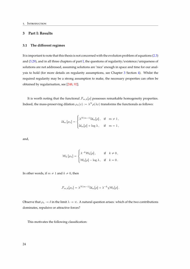
1. Introduction
3 Part I: Results
3.1 The different regimes
It is important to note that this thesis is not concernedwith the evolution problemof equations (2.3)
and (3.29), and in all three chapters of part I, the questions of regularity/existence/uniqueness of
solutions are not addressed, assuming solutions are ’nice’ enough in space and time for our anal-
ysis to hold (for more details on regularity assumptions, see Chapter 3 Section 4). Whilst the
required regularity may be a strong assumption to make, the necessary properties can often be
obtained by regularisation, see [248, 92].
It is worth noting that the functional Fm,krρs possesses remarkable homogeneity properties.
Indeed, the mass-preserving dilation ρλpxq :“ λNρpλxq transforms the functionals as follows:
Um rρλs “
$
’
&
’
%
λNpm´1qUmrρs , if m ‰ 1 ,
Umrρs ` log λ , if m “ 1 ,
and,
Wk rρλs “
$
’
&
’
%
λ´kWkrρs , if k ‰ 0 ,
Wkrρs ´ log λ , if k “ 0 .
In other words, ifm ‰ 1 and k ‰ 0, then
Fm,krρλs “ λNpm´1qUmrρs ` λ´kχWkrρs .
Observe that ρλ Ñ δ in the limit λÑ8. A natural question arises: which of the two contributions
dominates, repulsive or attractive forces?
This motivates the following classification:
24
3. Part I: Results
Definition 3.1 (Three different regimes).
Npm´ 1q ` k “ 0 This is the fair-competition regime, where homogeneities of the two competing con-
tributions exactly balance. If k ă 0, or equivalentlym ą 1, then we will have a dichotomy according
to χ (see Definition 3.7). Some variants of the HLS inequalities are very related to this dichotomy (see
Section 3.2). This was already proven in [136, 41, 71, 148] for the Keller–Segel case withN “ 2, and
in [39] for the Keller–Segel case with N ě 3. If k ą 0, that ism ă 1, no critical χ exists as we prove
in Chapter 2 Section 4.
Npm´ 1q ` k ą 0 This is the diffusion-dominated regime. Diffusion is strong, and is expected to over-
come aggregation, whatever χ ą 0 is. This domination effect means that solutions exist globally in
time and are bounded uniformly in time [61, 277, 276]. Stationary states were found by minimisa-
tion of the free energy functional in two and three dimensions [273, 78, 99] in the case of attractive
Newtonian potentials. Stationary states are radially symmetric if 2´N ď k ă 0 as proven in [89].
Moreover, in the particular case of N “ 2, k “ 0, and m ą 1 it has been proved in [89] that the
asymptotic behaviour is given by compactly supported stationary solutions independently of χ.
Npm´ 1q ` k ă 0 This is the attraction-dominated regime. This regime is less understood. Self-
attraction is strong, and can overcome the regularising effect of diffusion whatever χ ą 0 is, but
there also exist global in time regular solutions under some smallness assumptions, see [118, 275,
278, 109, 32, 110, 224, 65]. However, there is no complete criteria in the literature up to date distin-
guishing between the two behaviours. Most of the results known today deal with attractive Newtonian
interactions, that is k “ 2 ´N , in dimension N ě 3. For a study with linear diffusion m “ 1 and
k ă 0 in one dimension, see [65]. For the Newtonian case, global existence vs blow-up of weak solu-
tions has been investigated for the diffusion coefficients m “ 1 [118], 1 ă m ď 2 ´ 2N [275, 278],
m “ 2NN`2 [109], 2N
N`2 ă m ă 2 ´ 2N [110, 224] and for the whole range 0 ă m ď 2 ´ 2
N [32].
It was shown in [118] for linear diffusion m “ 1 that global in time weak solutions exist for initial
data with small enough LN2-norm, whereas there are no global smooth solutions with fast decay if
the second moment of the initial data is dominated by a power of the mass (with these two conditions
being incompatible). For diffusion coefficientm “ 2NN`2 making the free energy functional conformal
invariant, there exists a family of stationary solutions characterising the transition between blow-up
and global existence of radially symmetric weak solutions [109]. The case 2NN`2 ă m ă 2 ´ 2
N has
been studied in [110], where the authors suggest that the initial mass may not be an important quan-
tity to classify existence vs blow-up of solutions with the behaviour depending on the free energy, the
L2NpN`2q-norm and the second moment of the initial data. In [224], the authors proved a uniform
L8-bound for weak solutions in the range where these stationary solutions exist given the initial data
is uniformly bounded. As a consequence, uniqueness of weak solutions follows. We refer to [20] for a
discussion with more general interaction potentials in the aggregation-dominated regime.
25
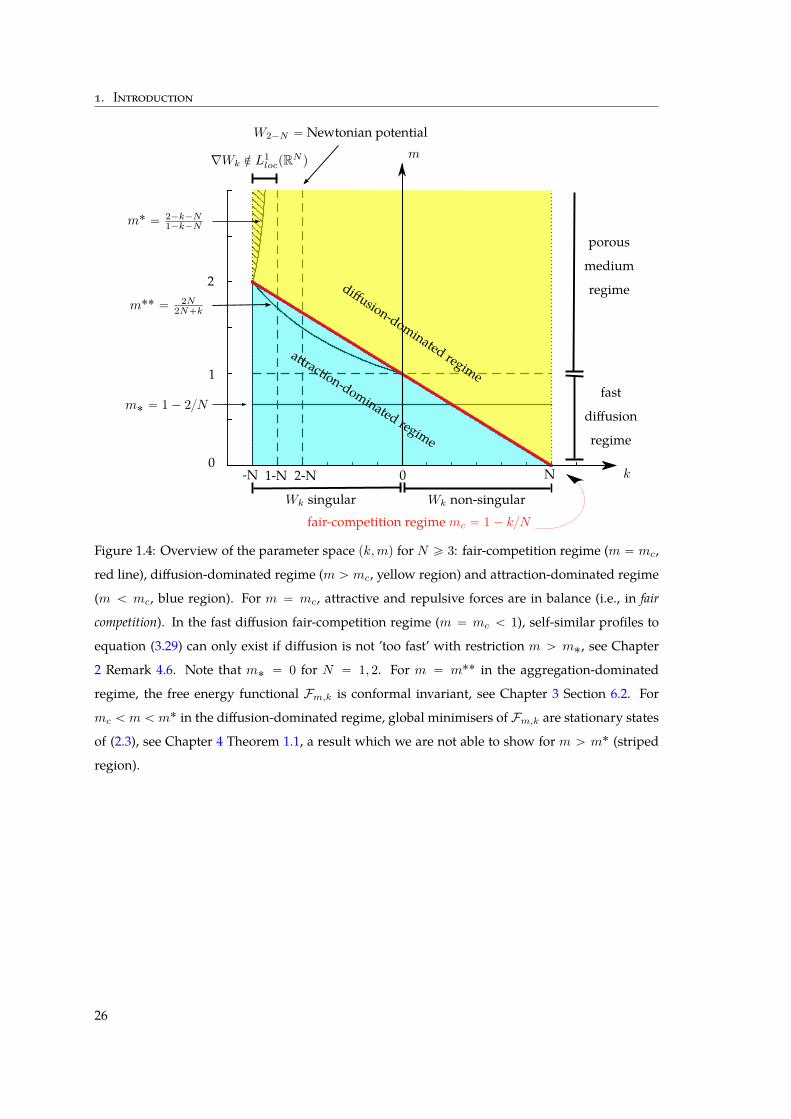
1. Introduction
diffusion-dominated regimeattraction-dominated regime
porous
medium
regime
fast
diffusion
regime
Wk singular Wk non-singular
-N 1-N 2-N 0 N
∇Wk R L1locpRN q
k
m
W2´N “ Newtonian potential
fair-competition regimemc “ 1´ kN
1
0
2
m˚ “ 1´ 2N
m˚˚ “ 2N2N`k
m˚ “ 2´k´N1´k´N
Figure 1.4: Overview of the parameter space pk,mq for N ě 3: fair-competition regime (m “ mc,
red line), diffusion-dominated regime (m ą mc, yellow region) and attraction-dominated regime
(m ă mc, blue region). For m “ mc, attractive and repulsive forces are in balance (i.e., in fair
competition). In the fast diffusion fair-competition regime (m “ mc ă 1), self-similar profiles to
equation (3.29) can only exist if diffusion is not ’too fast’ with restriction m ą m˚, see Chapter
2 Remark 4.6. Note that m˚ “ 0 for N “ 1, 2. For m “ m˚˚ in the aggregation-dominated
regime, the free energy functional Fm,k is conformal invariant, see Chapter 3 Section 6.2. For
mc ă m ă m˚ in the diffusion-dominated regime, global minimisers of Fm,k are stationary states
of (2.3), see Chapter 4 Theorem 1.1, a result which we are not able to show for m ą m˚ (striped
region).
26
3. Part I: Results
A word of caution is in place as to how the names of these three regimes are to be understood. We
introduced this terminology referring to the behaviour of the system with respect to blow-up and
so they describe the dominant behaviour that is to be expected when measures concentrate onto
a Dirac Delta. In light of these three regimes, we define the critical diffusion exponent as
mc :“ 1´ k
N.
Chapters 2 and 3 concentrate on the fair-competition regimem “ mc, whereas Chapter 4 focuses
on the diffusion-dominated regimem ą mc.
The family of non-local problems (2.3) has been intensively studied in various contexts arising
in physics and biology. The two-dimensional logarithmic case pm “ 1, k “ 0q is the so-called
Keller–Segel system in its simplest formulation [196, 197, 243, 194, 136, 41, 256], see Section 1. The
two- and three-dimensional configurations with Newtonian interaction pm “ 1, k “ 2 ´ Nq are
the so-called Smoluchowski-Poisson system arising in gravitational physics [105, 107, 106]. It de-
scribes macroscopically a density of particles subject to a self-sustained gravitational field.
Substituting linear diffusion by non-linear diffusion with m ą 1 in two dimensions and higher
is a way of regularising the Keller–Segel model as proved in [61, 277] where it is shown that so-
lutions exist globally in time regardless of the value of the parameter χ ą 0. It corresponds to
the diffusion-dominated case in two dimensions for which the existence of compactly supported
stationary states and global minimisers of the free energy has only been obtained quite recently
in [89]. The fair-competition case for Newtonian interaction k “ 2 ´ N was first clarified in [39],
see also [276], where the authors find that there is a similar dichotomy to the two-dimensional
classical Keller–Segel case pN “ 2,m “ 1, k “ 0q, choosing the non-local term as the Newtonian
potential, pN ě 3,m “ 2´2N, k “ 2´Nq. The main difference is that the stationary states found
for the critical case are compactly supported. We will see that such dichotomy also happens for
k ă 0 in our case while for k ą 0 the system behaves totally differently.
3.2 Variations of HLS inequalities
A key ingredient for the analysis in the case k ă 0 are certain functional inequalities which are
variants of the Hardy15-Littlewood16-Sobolev17 (HLS) inequality, also known as the weak Young’s
inequality [218, Theorem 4.3]:
15Godfrey Harold Hardy (1877-1947) was the most influential mathematician in Britain in the 20th century. He wrotealmost 100 papers together with Littlewood, considered to have been the most fruitful collaboration in the history ofmathematics. He was also a militant atheist and liked to talk of God as his personal enemy.
16John Edensor Littlewood (1885-1977) is a Britishmathematician, best known for his achievements in analysis, numbertheory, and differential equations. He practised his belief that mathematicians should take a vacation of at least 21 days ayear during which they should do no mathematics.
17Sergei Lvovich Sobolev (1908-1989) was a Soviet mathematician working in mathematical analysis and partial differ-ential equations.
27
1. Introduction
Theorem 3.2. Given k P p´N, 0q and p, q ą 1 satisfying
1p`
1q“ 2` k
N,
there exists an optimal constant CHLS “ CHLSpp, q, kq such that for all f P LppRN q and g P LqpRN q,ˇ
ˇ
ˇ
ˇ
ˇ
ˇ
ij
RNˆRN
|x´ y|kfpxqgpyq dxdy
ˇ
ˇ
ˇ
ˇ
ˇ
ˇ
ď CHLSfpgq . (3.21)
Inequality (3.21) (not in the sharp form) was proved in [180] and [181]. Thanks to Lieb [217],
the optimal constant CHLS is known explicitly if p “ q “ 2Np2N ` kq since in that case, it is
possible to explicitly compute the optimisers of (3.21), i.e. functions which, when inserted into
(3.21), give equality with the smallest constant. Indeed, optimisers for the sharp HLS inequality
p “ q are non-zero multiples of translations and dilations of
hpxq :“ˆ
11` |x|2
˙p2N`kq2.
In other words, the set of optimisers O to (3.21) is given by
O :“!
λh´x
s´ x0
¯
|λ P Rzt0u , s P Rą0 , x0 P RN)
In fact, the HLS optimisers play an important role: they are stationary states of the non-linear
Fokker–Planck equation (2.10) obtained from rescaling the fast diffusion (2.5) with diffusion ex-
ponent mpk,Nq :“ 1 ´ 2p2N ` kq. Note that indeed m˚ ă m ă 1 for all k P p´N, 0q, and so we
are in the range where the Barenblatt profile Gm (2.8) is well defined.
In the case p ‰ q on the other hand, optimisers to (3.21) exist, but neither the optimal constant
CHLS nor the optimisers are known explicitly.
As suggested by the connection between optimisers of the HLS inequality (3.21) and self-
similar solutions to the fast diffusion equation (2.5), there is a rich and fruitful interplay between
functional inequalities and non-linear partial differential equations [92, 125, 74, 133, 70, 132, 137]
that is still in the process of being discovered. Let us illustrate the kind of connection we might
want to exploit in our context with the example k “ 2´N in dimensionN ě 3. This is particularly
interesting since cN |x|2´N is the fundamental solution of the Laplacian,
cN |x|2´N ˚ f “ p´∆q´1f , cN :“ pp2´NqσN q´1
,
where σN :“ 2πN2Γ pN2q denotes the surface area of the N -dimensional unit ball. Therefore,
choosing p “ q “ 2Np2N ` kq “ 2NpN ` 2q in (3.21), we see that the sharp HLS inequality
encodes the smoothing properties of p´∆q´1 on RN .
28
3. Part I: Results
Let us rewrite the sharp HLS inequality (3.21) as Erf s ě 0 for f P L2NpN`2qpRN q, where the
so-called HLS functional E is given by
Erf s :“ CSf22NpN`2q ´
ż
RNfpxq
“
p´∆q´1f‰
pxq dx
with CS :“ cNCHLS “4
NpN´2qσ´2NN`1 given explicitly. Since the HLS optimisers O are the at-
tracting stationary states for a fast diffusion flow (2.11) with diffusion exponent m “ NpN ` 2q,
one might hope that the HLS functional E would be monotone decreasing along this flow. This is
indeed the case, and was shown in [74]: Fix some f P L2NpN`2qpRN q, f ě 0,ş
f dx “ş
Gm dx “ 1
satisfying (2.9) for someR ą 0, and let ρpt, xq be a solution of the fast diffusion equation (2.5) with
diffusion exponent m and ρp1, xq “ fpxq. Then, for all t ą 1, it follows that ddtErρptqs ď 0. For a
proof of this monotonicity relation, see [74, Theorem 2.1].
Further, using only the fast diffusion flow, rearrangement inequalities and the conformal invari-
ance of the HLS functional E , the authors in [74] were able to reprove the HLS inequality (3.21) for
the Newtonian case k “ 2 ´N , N ě 3. Their approach uses the fast diffusion flow to reduce the
HLS inequality to a Gagliardo-Nirenberg-Sobolev (GNS) inequality, which in turn reduces to the
Schwarz inequality. Note that the diffusion exponent m “ NpN ` 2q corresponds to the critical
exponent of the FDE related to the boundedness of the second moment of the stationary states
Gm and it plays a certain role in the long-time assymptotics of the FDE, see [101, 35].
A similar role is played by the logarithmic HLS inequality, established in its sharp version
in [77]:
Theorem 3.3. Let k “ 0, m “ 1. For all non-negative measurable functions f P L1pRN q such that
f log f, f logp1` |x|2q P L1pRN q, we have
´χ
ij
RNˆRN
fpxqlog |x´ y|fpyqdxdy ď 1N
ż
RNfpxq log fpxqdx` C0, (3.22)
where the optimal constant C0 “ C0pNq is given by
C0pNq :“ 12 log π ` 1
Nlog
˜
Γ`
N2˘
Γ pNq
¸
`12
ˆ
ψpNq ´ ψ
ˆ
N
2
˙˙
.
Here ψ denotes the logarithmic derivative of the Γ-function.
Carlen and Loss, together with Beckner, have demonstrated that the logarithmic HLS inequal-
ity is also a consequence of (3.21) as k Ñ 0, see [77].
Further, the sharp logarithmic HLS inequality on R2 can be obtained by a similar fast diffusion
flow argument as we discussed above for the HLS inequality (3.21) [74], an approach which is
facilitated by the fact that the logarithmic HLS functional is invariant under scalings. It can also
29
1. Introduction
be derived by optimal transport techniques in one dimension and in the two-dimensional radial
setting [62], using techniques which we will adapt for our context in Chapter 2 and Chapter 3.
The above examples illustrate the intrinsic relationship between functional inequalities, their
minimisers, and certain non-linear diffusion equations. We will make use of these connections in
Part I when studying the stationary states to the aggregation-diffusion equations (2.3) and (3.29).
We will now state the new functional inequalities derived in this thesis.
Theorem 3.4. Let k P p´N, 0q, andm ě mc. For f P L1pRN q X LmpRN q, we haveˇ
ˇ
ˇ
ˇ
ˇ
ˇ
ij
RNˆRN
|x´ y|kfpxqfpyqdxdy
ˇ
ˇ
ˇ
ˇ
ˇ
ˇ
ď C˚||f ||pk`NqN1 ||f ||mcmc , (3.23)
where the optimal constant C˚ is given by
C˚pN, k,mq :“ supf‰0
$
&
%
ˇ
ˇ
ˇ
ť
RNˆRN |x´ y|kfpxqfpyqdxdy
ˇ
ˇ
ˇ
||f ||pk`NqN1 ||f ||mcmc
, f P L1pRN q X LmpRN q
,
.
-
ă 8.
Proof. The inequality is a direct consequence of Theorem 3.2 by choosing p “ q “ 2Np2N ` kq,
and of Hölder’s inequality. More precisely, for any f P L1pRN q X LmpRN qwithm ą mc, we haveˇ
ˇ
ˇ
ˇ
ˇ
ˇ
ij
RNˆRN
|x´ y|kfpxqfpyqdxdy
ˇ
ˇ
ˇ
ˇ
ˇ
ˇ
ď CHLS ||f ||2p ď CHLS ||f ||
α1 ||f ||
βm.
with
α “ 2´ β , β “ 2ˆ
1´ pp
˙ˆ
m
1´m
˙
“
ˆ
k
N
˙ˆ
m
1´m
˙
.
Choosingm “ mc, we have α “ 1`kN , β “ mc, and hence (3.23) follows with C˚ “ C˚pk,m,Nq
finite and bounded from above by CHLS .
Further, we will obtain as a by-product of our investigations the following one-dimensional
HLS-type inequality involving a second moment term:
Theorem 3.5. Let k P p´N, 0q and m “ mc. For any 0 ă χ ă C´1˚ , there exists an optimal constant
C “ Cpk,N, χq such that
χ
ij
RNˆRN
|x´ y|kfpxqfpyq dxdy ď C ` fmcmc `p´kq
2
ż
RN|x|2fpxq dx (3.24)
for all f P L1pRN q X LmcpRN q with f1 “ 1,ş
xfpxq dx “ 0 and |x|2fpxq P L1pRN q. If N “ 1, then
the set of optimisers is the unique self-similar solution to equation (2.3).
Moreover, we will prove the analogue version of the above functional inequality for positive
0 ă k ă 23 in one dimension, corresponding to a reversed HLS-type inequality with a second
moment term:
30
3. Part I: Results
Theorem 3.6. Let N “ 1, k P p0, 23q andmc :“ 1´ k. For any χ ą 0, there exists an optimal constant
C “ Cpk, χq such that
χ
ij
RˆR
|x´ y|kfpxqfpyq dxdy `k
2
ż
R|x|2fpxq dx ě C `
ż
Rfmcpxq dx (3.25)
for all f P L1pRqXLmcpRqwith f1 “ 1,ş
xfpxq dx “ 0 and`
|x|2 ` |x|k˘
fpxq P L1pRq. The optimiser
is given by the unique self-similar solution to equation (2.3).
Up to our knowledge, the functional inequalities (3.24) and (3.25) are not known in the litera-
ture.
The analysis of the free energy functionals Fm,k and their respective gradient flows is closely
related to HLS-type inequalities [218, 163, 74, 39]. To give a flavour, we highlight the case pm “
1, k “ 0q, called the logarithmic case. It is known from [136, 41] using [77, 19] that the functional
F1,0 is bounded from below if and only if 0 ă χ ď 1. Moreover, F1,0 achieves its minimum if and
only if χ “ 1 and the extremal functions are mass-preserving dilations of Cauchy’s density:
ρ0pxq “1π
ˆ
11` |x|2
˙
. (3.26)
In [77], the authors have proved the uniqueness (up to dilations and translations) of this logarith-
mic HLS inequality based on a competing-symmetries argument. We develop in Chapter 3 an
alternative argument based on some accurate use of the Jensen’s inequality to extend these results
to the case N “ 1, k P p´1, 0q and m “ mc. This goal will be achieved for the variant of the HLS
inequality (3.23) as in [39], indeed being a combination of the HLS inequality and interpolation
estimates.
In Chapter 3, we develop a strategy which enables to recover directly inequalities (3.22), (3.23),
(3.24) and (3.25). Our method involves two main ingredients:
• First it is required to know a priori that the inequality possesses some extremal function
denoted e.g. by ρpxq (characterised as a critical point of the energy functional). This is not
an obvious task due to the intricacy of the equation satisfied by ρpxq. Without this a priori
knowledge, the proof of the inequality remains incomplete. The situation is in fact similar
to the case of convex functionals, where the existence of a critical point ensures that it is a
global minimiser of the functional.
• Second we invoke convexity inequalities related to Jensen’s inequality.
31
1. Introduction
3.3 The fair-competition regime
In the fair-competition regime, when m “ mc “ 1 ´ kN , we denote the corresponding energy
functional by Fkrρs “ F1´kN,krρs. Notice that the functional Fk is homogeneous in this regime,
i.e. for dilations ρλpxq :“ λNρpλxq, we have
Fkrρλs “ λ´kFkrρs . (3.27)
In fact, using the Euler18 theorem for homogeneous functions, we can show that for k P p´N, 0q
any stationary state of the aggregation-diffusion equation (2.3) with bounded second moment
has zero energy (see Chapter 2, Lemma 3.2). This argument does not apply in the logarithmic
case k “ 0 and it allows us here to make the connection between global minimisers of Fk and
stationary states of (2.3) for k ă 0. Indeed, for any ρ P Y , where
Y :“"
ρ P L1`
`
RN˘
X Lm`
RN˘
: ||ρ||1 “ 1 ,ż
xρpxq dx “ 0*
,
and for any χ ą 0, we can rewrite the functional inequality (3.23) as follows:
Fkrρs ě1´ χC˚Npm´ 1q ||ρ||
mm ,
where C˚ “ C˚pk,Nq is the optimal constant defined in (3.23). Since the energy of the global
minimisers is always smaller or equal to the energy of the stationary states, and stationary states
have zero energy as mentioned above, it follows that χ ě 1C˚. We define the critical interaction
strength by
χcpk,Nq :“ 1C˚pk,Nq
. (3.28)
Hence, for χ “ χc, all stationary states of equation (2.3) are global minimisers of Fk. We can also
directly see that for 0 ă χ ă χc, no stationary states exist. Showing that stationary states of an
equation are globalminimisers of the associated energy functional is usually themore challenging
implication. The converse is trivial for systems that exhibit a gradient flow structure (2.19) since
global minimisers are critical points of the energy functional, i.e. the first variation of the energy
functional vanishes at these points, and therefore global minimisers are automatically stationary
states. It remains then to verify that global minimisers of Fk are regular enough to be station-
ary states of equation (2.3). Showing the good regularity properties can be challenging, and it is
proven and explained in detail in Chapter 2.
The case k ą 0 has been a lot less studied, and we will show in Chapter 2 that no critical inter-
action strength exists as there is no χ ą 0 for which Fk admits global minimisers. On the other
hand, we observe certain similarities with the behaviour of the fast diffusion equation (0 ă m ă 1,
χ “ 0) [287].18Leonhard Euler (1707-1783), born in Switzerland and deceased in Russia, was one of the most influential and prolific
mathematicians in history with more than 800 papers bearing his name. He was blind for the last 15 years of his life,during which time he nevertheless wrote over 300 papers.
32
3. Part I: Results
From these observations, one can see that the analysis in the fair-competition regime depends
on the sign of k. We give a short overview of the differences between the cases k ă 0, k “ 0, k ą 0
in the definition below, including new insights obtained in this thesis:
Definition 3.7 (Three different cases in the fair-competition regime).
k ă 0 This is the porous medium case with m P p1, 2q, where diffusion is small in regions of small
densities. The classical porous medium equation, i.e. χ “ 0, is very well studied, see [289] and the
references therein. Here, we have a dichotomy for existence of stationary states and global minimisers of
the energy functional Fk depending on the critical parameter χc defined in (3.28), and hence separate
the sub-critical, the critical and the super-critical case, according to χ ž χc.
k “ 0 This is the logarithmic case. There exists an explicit extremal density ρ0 given in (3.26) which
realises the minimum of the functionalF0 when χ “ 1. Moreover, the functionalF0 is bounded below
but does not achieve its infimum for 0 ă χ ă 1 while it is not bounded below for χ ą 1. Hence,
χc “ 1 is the critical parameter in the logarithmic case whose asymptotic behaviour was analysed
in [62] in one dimension and radial initial data in two dimensions. We refer to the results in [71, 148]
for the two dimensional case.
k ą 0 This is the fast diffusion case with m P p0, 1q, where diffusion is strong in regions of small den-
sities. For any χ ą 0, no radially symmetric non-increasing stationary states with bounded kth
moment exist, and Fk has no radially symmetric non-increasing minimisers. However, we have ex-
istence of self-similar profiles independently of χ ą 0 as long as diffusion is not too fast, i.e. k ď 1.
Self-similar profiles can only exist if diffusion is not too strong with restriction 0 ă k ă 2, that is
pN ´ 2qN ă m ă 1.
3.3.1 Change of variables
As mentioned above, for certain choices of m, k and χ, there are no stationary states to (2.3),
see Section 3.3.2. This is known in the case of the sub-critical classical Keller–Segel model in two
dimensions [41] for instance. If there are no stationary states, the scale invariance of (2.3)motivates
us to look for self-similar solutions instead. To this end, we rescale equation (2.3) to a non-linear
Fokker–Planck-type equation as in explained in Section 2.1.3 in the context of the non-linear heat
equation. Let us define
upt, xq :“ αN ptqρ pβptq, αptqxq ,
where ρpt, xq solves (2.3) and the functions αptq, βptq are to be determined. If we assume up0, xq “
ρp0, xq, then upt, xq satisfies the rescaled aggregation-diffusion equation$
’
&
’
%
Btu “1N∆um ` 2χ∇ ¨ pu∇Skq `∇ ¨ pxuq , t ą 0 , x P RN ,
upt “ 0, xq “ ρ0pxq ě 0 ,ż 8
´8
ρ0pxq dx “ 1 ,ż 8
´8
xρ0pxq dx “ 0 ,(3.29)
33
1. Introduction
for the choices
αptq “ et, βptq “
$
’
&
’
%
12´k
`
ep2´kqt ´ 1˘
, if k ‰ 2,
t, if k “ 2,
and with ∇Sk given by (2.17) with u instead of ρ. By differentiating the centre of mass of u, we
see easily thatż
RNxupt, xq dx “ e´t
ż
RNxρ0pxq dx “ 0 , @t ą 0 ,
and so the initial zero centre of mass is preserved for all times. Self-similar solutions to (2.3) now
correspond to stationary solutions of (3.29).
From now on, we switch notation from u to ρ for simplicity, it should be clear from the context if
we are in original or rescaled variables.
In rescaled variables, equation (3.29) is the formal gradient flow of the rescaled free energy
functional Fk,resc, which is complemented with an additional quadratic confinement potential,
Fk,rescrρs “ Fkrρs `12Vrρs , Vrρs “
ż
RN|x|2ρpxq dx .
Defining the sets
Y2 :“ tρ P Y : Vrρs ă 8u , Yk :“"
ρ P Y :ż
RN|x|kρpxq dx ă 8
*
,
we see that Fk,resc is well-defined and finite on Y2 for k ă 0 and on Y2,k :“ Y2 XYk for k ą 0. Just
like the original equation (2.3), the rescaled system (3.29) has a formal gradient flow structure in
the Euclidean Wasserstein metric W, and so we can write (3.29) as
Btρ “ ∇ ¨ pρ∇Tk,rescrρsq “ ´∇WFk,rescrρs ,
where Tk,resc denotes the first variation of the rescaled energy functional,
Tk,rescrρspxq :“ Tkrρspxq `|x|2
2
with Tk as defined in (2.20).
3.3.2 Main results Chapter 2
In Chapter 2, we analyse the properties of the functional Fk, its global minimisers, and its relation
to stationary states of (2.3) for the fair-competition regime in any dimension N ě 1. For the
porous medium case k ă 0, we show a similar dichotomy to [39] in the whole range k P p´N, 0q
including the most singular cases ´N ă k ď 1 ´ N . We show that stationary states exist only
for a critical value of χ “ χc with χc given by (3.28) and that they are compactly supported,
bounded, radially symmetric decreasing and continuous functions. Moreover, we show that they
34
3. Part I: Results
are global minimisers of Fk. Next, we analyse the sub-critical case χ ă χc in rescaled variables
andwe show the existence of global minimisers for the rescaled free energy functional Fk,resc with
the properties above leading to the existence of self-similar solutions in original variables. Let us
mention that the regularity results for global minimisers of Fk and Fk,resc need a careful treatment
of the problem in radial coordinates involving non-trivial properties of hypergeometric functions,
particularly in the singular regime´N ă k ď 1´N when additional Hölder regularity C0,αpRN q
with α P p1 ´ k ´ N, 1q is needed for the gradient ∇Sk to be well defined. The properties of the
kernel in radial coordinates are postponed to the Appendix A of Chapter 2.
In Section 4 of Chapter 2, we analyse the fast diffusion case k ą 0. Let us mention that, to
the best of our knowledge, there are no results in the literature concerning the case k P p0, Nq in
which 0 ă mc “ 1 ´ kN ă 1. There is one related result in [116] for the limiting case in one
dimension taking m “ 0, corresponding to logarithmic diffusion, and k “ 1. In that case, there
is no criticality present as solutions to (2.3) with pm “ 0, k “ 1q are globally defined in time for
all values of the parameter χ ą 0. We show that no radially symmetric non-increasing stationary
states and no radially symmetric non-increasing global minimisers exist in original variables for
all values of the critical parameter χ and for k P p0, Nq while we establish the existence of sta-
tionary states for all values of the critical parameter χ in rescaled variables for k P p0, 1s. In this
sense, there is no criticality for k ą 0. However, we have not analysed the minimisation problem
for Fk,resc directly for arbitrary dimension N ě 1 as we did for the case k ă 0. A full proof of
non-criticality involves the analysis of the minimisation problem in rescaled variables showing
that global minimisers exist in the right functional spaces for all values of the critical parameter
and that they are indeed stationary states. This will be proved in one dimension in Chapter 3 by
optimal transport techniques and postponed for further future investigations in general dimen-
sion. We finally illustrate these results by numerical experiments in one dimension corroborating
the absence of critical behaviour for k ą 0.
More precisely, we will prove the following main theorems in Chapter 2:
Theorem 3.8 (The Critical Porous Medium Regime). In the porous medium regime k P p´N, 0q and
for critical interaction strengths χ “ χc, there exist global minimisers of Fk and they are radially sym-
metric non-increasing, compactly supported and uniformly bounded. Furthermore, all stationary states
with bounded second moment are global minimisers of the energy functional Fk, and conversely, all global
minimisers of Fk are stationary states of (2.3).
Theorem 3.9 (The Sub-Critical Porous Medium Regime). In the porous medium regime k P p´N, 0q
and for sub-critical interaction strengths 0 ă χ ă χc, no stationary states exist for equation (2.3) and
no minimisers exist for Fk. In rescaled variables, all stationary states are continuous and compactly sup-
35
1. Introduction
ported. There exist global minimisers of Fk,resc and they are radially symmetric non-increasing and uni-
formly bounded stationary states of equation (3.29).
Due to the homogeneity (3.27) of the functional Fk, each global minimiser gives rise to a family
of global minimisers for χ “ χc by dilation since they have zero energy. It is an open problem to
show that there is a unique global minimiser for χ “ χc modulo dilations. This uniqueness was
proven in the Newtonian case in [302], and for any k P p´1, 0q for the one-dimensional case in
Chapter 3.
In contrast, in rescaled variables, we do not know if stationary states with bounded second
moment are among global minimisers of Fk,resc for the sub-critical case 0 ă χ ă χc except in one
dimension, see Chapter 3. It is also an open problem to show the uniqueness of radially symmetric
stationary states of the rescaled equation (3.29) for N ě 2.
Theorem 3.10 (The Fast Diffusion Regime). In the fast diffusion regime k P p0, Nq equation (2.3)
has no radially symmetric non-increasing stationary states with kth moment bounded, and there are no
radially symmetric non-increasing global minimisers for the energy functionalFk for anyχ ą 0. In rescaled
variables, radially symmetric non-increasing stationary states can only exist if 0 ă k ă 2, that is pN ´
2qN ă mc ă 1. Similarly, global minimisers with finite energy Fk,resc can only exist in the range 0 ă k ă
2Np2 ` Nq, that is Np2 ` Nq ă mc ă 1. For k P p0, 1s, there exists a continuous radially symmetric
non-increasing stationary state of the rescaled equation (3.29).
3.3.3 Main results Chapter 3
Chapter 3 focuses on the one-dimensional fair-competition regime. We will make a survey of
the main results known in one dimension about the stationary states of the aggregation-diffusion
equation and globalminimisers of the associated energy functionals in the fair-competition regime
while at the same time providing newmaterial in one dimensionwith alternative proofs and infor-
mation about long time asymptotics which are not known yet in higher dimensions. The novelties
will be showing the functional inequalities (3.23) for m “ mc, (3.24) and (3.25) independently of
the flow and studying the long-time asymptotics of the equations (2.3) and (3.29) by exploiting
the one dimensional setting. More precisely, we will make accurate use of the expression for the
dissipation of the Wasserstein distance derived in Theorem 4.1, which is only valid in one dimen-
sion. A similar identity to (??) can also be derived for the radial setting in higher dimension, which
opens up opportunities to generalise our one-dimensional results. Let us stress that we did not
develop any theory of the evolution problem as mentioned before, and in this sense, the conver-
gence results in this chapter remain formal, assuming that solutions ρpt, xq are regular enough for
our computations to hold.
36
3. Part I: Results
In the sub-critical and critical porous medium regime, we will demonstrate convergence to
equilibrium in Wasserstein distance under a certain stability condition, a restriction which is not
necessary for the asymptotic behaviour in the fast diffusion regime. More precisely, the required
stability condition is a uniform W2,8pRq-stability estimate on the Brenier map ψpt, xqwhose gra-
dient pushes forward a solution ρpt, xq onto a stationary state, ρpt, xq dx “ Bxψpt, xq#ρpxq dx:
Bxxψpt, xq P L8 pR`, L8pRqq such that ||Bxxψ||L8pR`,L8pRqq ď 1` 1
m.
For the sub-critical porous medium regime, and for the fast diffusion regime, we obtain exponen-
tial convergence to self-similar profiles with an explicit rate which does not depend on the interac-
tion strength χ. This is remarkable in the sub-critical case χ ă χc as it means that the asymptotic
behaviour does not change as χ approaches χc from below, whilst the behaviour at χ “ χc is very
different with the existence of infinitely many stationary states that act as attractors for a certain
class of solutions. This effect appeared in the logarithmic case (k “ 0,m “ 1) analysed in [62].
Finally, we provide numerical simulations of system (2.3) to illustrate the properties of equi-
libria and self-similar profiles in the different parameter regimes for the fair-competition regime.
We use a Jordan-Kinderlehrer-Otto (JKO) steepest descent scheme [195, 248] which was proposed
in [36] for the logarithmic case k “ 0, and generalised to the porous-medium case k P p´1, 0q
in [67]. It can easily be extended to rescaled variables and works just in the same way in the fast
diffusion regime k P p0, 1q.
For the logarithmic case k “ 0, m “ 1, we know that the critical interaction strength is given by
χc “ 1 separating the blow-up regime from the regime where self-similar solutions exist [136, 41,
33]. As shown in Chapter 2, there is no critical interaction strength for the fast diffusion regime
k ą 0, however the dichotomy appears in the porous medium regime k ă 0. It is not known
how to compute the critical parameter χcpkq explicitly for k ă 0, however, we can make use of the
numerical scheme to compute χc numerically.
Figure 1.5 gives an overview of the behaviour of solutions. In the red region, we observe finite-
time blow-up of solutions, whereas for a choice of pk, χq in the green region, solutions converge
exponentially fast to a unique self-similar profile. The critical regime is characterised by the black
line χcpkq with ´1 ă k ď 0, separating the grey from the white region. Note that numerically we
have χcp´0.99q “ 0.11 and χcp0q “ 1. Figure 1.5 has been created by solving the rescaled equa-
tion (3.29) repeatedly for each k from ´0.99 to 0 in 0.01 steps. For a given k, the numerical critical
interaction strength χcpkq is defined to be the largest χ for which the numerical solution can be
computed without blow-up until the L2-error between two consecutive solutions is less than a
specified tolerance. In Chapter 3, we describe in detail the numerical scheme and investigate the
behaviour of solutions at selected points in the parameter space pk, χq.
37
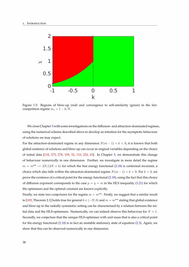
1. Introduction
Figure 1.5: Regions of blow-up (red) and convergence to self-similarity (green) in the fair-competition regimemc “ 1´ kN .
We closeChapter 3with some investigations on the diffusion- and attraction-dominated regimes,
using the numerical scheme described above to develop an intuition for the asymptotic behaviour
of solutions we may expect.
For the attraction-dominated regime in any dimension Npm ´ 1q ` k ă 0, it is known that both
global existence of solutions and blow-up can occur in original variables depending on the choice
of initial data [118, 275, 278, 109, 32, 110, 224, 65]. In Chapter 3, we demonstrate this change
of behaviour numerically in one dimension. Further, we investigate in more detail the regime
m “ m˚˚ :“ 2Np2N ` kq for which the free energy functional (2.18) is conformal invariant, a
choice which also falls within the attraction-dominated regime Npm ´ 1q ` k ă 0. For k ă 0, we
prove the existence of a critical point for the energy functional (2.18), using the fact that this choice
of diffusion exponent corresponds to the case p “ q “ m in the HLS inequality (3.21) for which
the optimisers and the optimal constant are known explicitly.
Finally, we state two conjectures for the regimem “ m˚˚. Firstly, we suggest that a similar result
to [109, Theorem 2.1] holds true for general k P p´N, 0q andm “ m˚˚ stating that global existence
and blow-up in the radially symmetric setting can be characterised by a relation between the ini-
tial data and the HLS-optimisers. Numerically, we can indeed observe this behaviour for N “ 1.
Secondly, we conjecture that the unique HLS-optimiser with unit mass that is also a critical point
for the energy functional (2.18) is in fact an unstable stationary state of equation (2.3). Again, we
show that this can be observed numerically in one dimension.
38
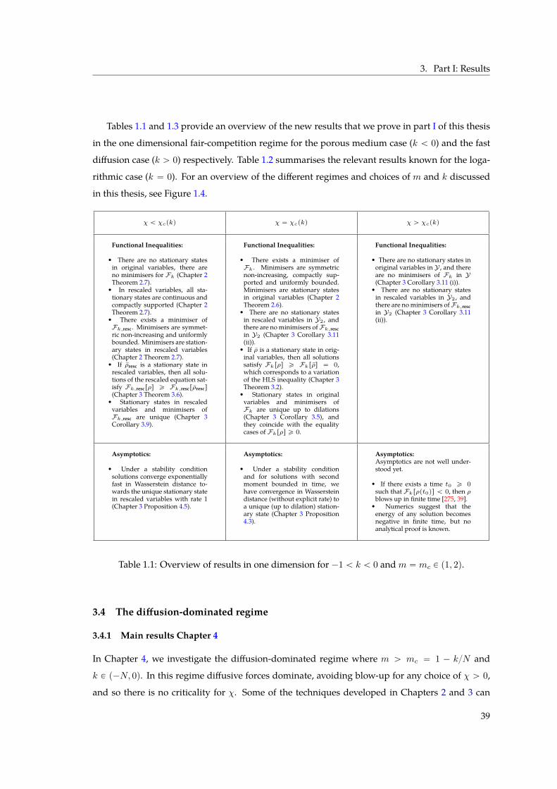
3. Part I: Results
Tables 1.1 and 1.3 provide an overview of the new results that we prove in part I of this thesis
in the one dimensional fair-competition regime for the porous medium case (k ă 0) and the fast
diffusion case (k ą 0) respectively. Table 1.2 summarises the relevant results known for the loga-
rithmic case (k “ 0). For an overview of the different regimes and choices of m and k discussed
in this thesis, see Figure 1.4.
χ ă χcpkq χ “ χcpkq χ ą χcpkq
Functional Inequalities:
• There are no stationary statesin original variables, there areno minimisers for Fk (Chapter 2Theorem 2.7).
• In rescaled variables, all sta-tionary states are continuous andcompactly supported (Chapter 2Theorem 2.7).
• There exists a minimiser ofFk,resc. Minimisers are symmet-ric non-increasing and uniformlybounded. Minimisers are station-ary states in rescaled variables(Chapter 2 Theorem 2.7).
• If ρresc is a stationary state inrescaled variables, then all solu-tions of the rescaled equation sat-isfy Fk,rescrρs ě Fk,rescrρrescs(Chapter 3 Theorem 3.6).
• Stationary states in rescaledvariables and minimisers ofFk,resc are unique (Chapter 3Corollary 3.9).
Functional Inequalities:
• There exists a minimiser ofFk . Minimisers are symmetricnon-increasing, compactly sup-ported and uniformly bounded.Minimisers are stationary statesin original variables (Chapter 2Theorem 2.6).
• There are no stationary statesin rescaled variables in Y2, andthere are nominimisers of Fk,rescin Y2 (Chapter 3 Corollary 3.11(ii)).
• If ρ is a stationary state in orig-inal variables, then all solutionssatisfy Fkrρs ě Fkrρs “ 0,which corresponds to a variationof the HLS inequality (Chapter 3Theorem 3.2).
• Stationary states in originalvariables and minimisers ofFk are unique up to dilations(Chapter 3 Corollary 3.5), andthey coincide with the equalitycases of Fkrρs ě 0.
Functional Inequalities:
• There are no stationary states inoriginal variables in Y , and thereare no minimisers of Fk in Y(Chapter 3 Corollary 3.11 (i)).
• There are no stationary statesin rescaled variables in Y2, andthere are nominimisers of Fk,rescin Y2 (Chapter 3 Corollary 3.11(ii)).
Asymptotics:
• Under a stability conditionsolutions converge exponentiallyfast in Wasserstein distance to-wards the unique stationary statein rescaled variables with rate 1(Chapter 3 Proposition 4.5).
Asymptotics:
• Under a stability conditionand for solutions with secondmoment bounded in time, wehave convergence in Wassersteindistance (without explicit rate) toa unique (up to dilation) station-ary state (Chapter 3 Proposition4.3).
Asymptotics:Asymptotics are not well under-stood yet.
• If there exists a time t0 ě 0such that Fkrρpt0qs ă 0, then ρblows up in finite time [275, 39].
• Numerics suggest that theenergy of any solution becomesnegative in finite time, but noanalytical proof is known.
Table 1.1: Overview of results in one dimension for ´1 ă k ă 0 andm “ mc P p1, 2q.
3.4 The diffusion-dominated regime
3.4.1 Main results Chapter 4
In Chapter 4, we investigate the diffusion-dominated regime where m ą mc “ 1 ´ kN and
k P p´N, 0q. In this regime diffusive forces dominate, avoiding blow-up for any choice of χ ą 0,
and so there is no criticality for χ. Some of the techniques developed in Chapters 2 and 3 can
39
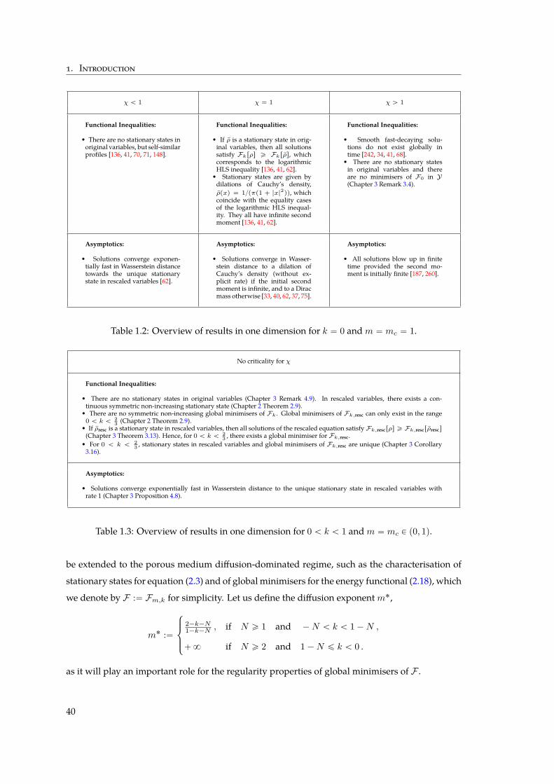
1. Introduction
χ ă 1 χ “ 1 χ ą 1
Functional Inequalities:
• There are no stationary states inoriginal variables, but self-similarprofiles [136, 41, 70, 71, 148].
Functional Inequalities:
• If ρ is a stationary state in orig-inal variables, then all solutionssatisfy Fkrρs ě Fkrρs, whichcorresponds to the logarithmicHLS inequality [136, 41, 62].
• Stationary states are given bydilations of Cauchy’s density,ρpxq “ 1pπp1 ` |x|2qq, whichcoincide with the equality casesof the logarithmic HLS inequal-ity. They all have infinite secondmoment [136, 41, 62].
Functional Inequalities:
• Smooth fast-decaying solu-tions do not exist globally intime [242, 34, 41, 68].
• There are no stationary statesin original variables and thereare no minimisers of F0 in Y(Chapter 3 Remark 3.4).
Asymptotics:
• Solutions converge exponen-tially fast in Wasserstein distancetowards the unique stationarystate in rescaled variables [62].
Asymptotics:
• Solutions converge in Wasser-stein distance to a dilation ofCauchy’s density (without ex-plicit rate) if the initial secondmoment is infinite, and to a Diracmass otherwise [33, 40, 62, 37, 75].
Asymptotics:
• All solutions blow up in finitetime provided the second mo-ment is initially finite [187, 260].
Table 1.2: Overview of results in one dimension for k “ 0 andm “ mc “ 1.
No criticality for χ
Functional Inequalities:
• There are no stationary states in original variables (Chapter 3 Remark 4.9). In rescaled variables, there exists a con-tinuous symmetric non-increasing stationary state (Chapter 2 Theorem 2.9).
• There are no symmetric non-increasing global minimisers of Fk . Global minimisers of Fk,resc can only exist in the range0 ă k ă 2
3 (Chapter 2 Theorem 2.9).• If ρresc is a stationary state in rescaled variables, then all solutions of the rescaled equation satisfy Fk,rescrρs ě Fk,rescrρrescs(Chapter 3 Theorem 3.13). Hence, for 0 ă k ă 2
3 , there exists a global minimiser for Fk,resc.• For 0 ă k ă 2
3 , stationary states in rescaled variables and global minimisers of Fk,resc are unique (Chapter 3 Corollary3.16).
Asymptotics:
• Solutions converge exponentially fast in Wasserstein distance to the unique stationary state in rescaled variables withrate 1 (Chapter 3 Proposition 4.8).
Table 1.3: Overview of results in one dimension for 0 ă k ă 1 andm “ mc P p0, 1q.
be extended to the porous medium diffusion-dominated regime, such as the characterisation of
stationary states for equation (2.3) and of global minimisers for the energy functional (2.18), which
we denote by F :“ Fm,k for simplicity. Let us define the diffusion exponentm˚,
m˚ :“
$
’
&
’
%
2´k´N1´k´N , if N ě 1 and ´N ă k ă 1´N ,
`8 if N ě 2 and 1´N ď k ă 0 .
as it will play an important role for the regularity properties of global minimisers of F .
40
3. Part I: Results
First of all, we show in Chapter 4 that stationary states of (2.3) in Y are radially symmetric for
all χ ą 0, k P p´N, 0q and m ą mc. This is one of the main results of [89], and is achieved under
the assumption that the interaction kernelWk is not more singular than the Newtonian potential
close to the origin. The proof in [89] can be adapted to our setting as the main arguments con-
tinue to hold even for more singularWk. Let us mention that the radiality of stationary states is
crucial when making the connection to global minimisers of F , which are also radially symmetric
as the energy decreases under taking symmetric decreasing rearrangements19. In other words, this
result reduces the question of uniqueness of stationary states to uniqueness of radially symmetric
stationary states, allowing us to work in the radial setting instead.
Investigating the properties of global minimisers for F , we show in Chapter 4 that they are com-
pactly supported and uniformly bounded for all χ ą 0, k P p´N, 0q and m ą mc. Note that
this result corresponds to what we find in the critical porous medium fair-competition regime,
see Theorem 3.8. However here, we choose to develop a new method for the proof: instead of an
iterative argument using hypergeometric functions to control global minimisers at the origin di-
rectly (see Chapter 2), we first proof an estimate for the mean-field potential Sk “Wk ˚ρ, and then
argue by contradiction. The idea is that for every unbounded global minimiser one can construct
a bounded competitor that decreases the energy. The difficulty in handling terms involving hy-
pergeometric functions remains the same. Existence of global minimisers can be obtained using
the concentration compactness argument by Lions [220], whereas proving Hölder regularity in
the singular range ´N ă k ď 1´N turns out to be more challenging in the diffusion-dominated
case as one may have diffusion exponents m that are greater than 2, in which case one cannot
transfer Hölder regularity of ρm´1 to ρ directly. We obtain that global minimisers of F are regular
enough to be stationary states of equation (2.3) under the condition that diffusion is not too fast,
mc ă m ă m˚. Moreover, bootstrapping on the obtained regularity using the Euler18-Lagrange20
equation, we obtain that global minimisers of F in Y are C8 inside their support.
Finally, we apply the same methods as in Chapter 3 to derive an HLS-type inequality in one di-
mension using optimal transport techniques, establishing equivalence between global minimisers
of F in Y and stationary states of equation (2.3). Additionally, this functional inequality provides
uniqueness of stationary states in one dimension.
In summary, we will prove the following results in Chapter 4:
19The function ρ# is said to be the symmetric decreasing rearrangement of ρ if ρ# is radially symmetric non-increasingwith the level sets of ρ# and ρ having the same measure, i.e. |tx : ρ#pxq ą cu| “ |tx : ρpxq ą cu|.
20Joseph Louis Lagrange (1736-1813)was an Italian-Frenchmathematician and astronomer. Lagrangewas only 19 yearsold when he wrote to Euler announcing a new formalism to simplify Euler’s method for finding a curve that satisfies anextremum condition. Using this formalism, he derived the fundamental equation of the calculus of variations, knowntoday as Euler-Lagrange equation.
41
1. Introduction
Theorem 3.11. Let N ě 1, χ ą 0 and k P p´N, 0q. All stationary states of equation (1.2) are radially
symmetric decreasing. If m ą mc, then there exists a global minimiser ρ of F on Y . Further, all global
minimisers ρ P Y are radially symmetric non-increasing, compactly supported, uniformly bounded and
C8 inside their support. Moreover, all global minimisers of F are stationary states of (1.2) whenever
mc ă m ă m˚. Finally, ifmc ă m ă 2, we have ρ P W1,8 `
RN˘
.
Theorem 3.12. Let N “ 1, χ ą 0 and k P p´1, 0q. All stationary states of (1.2) are global minimisers of
the energy functional F on Y . Further, stationary states of (1.2) in Y are unique.
4 Part I: Perspectives
There are many interesting open problems of varying difficulty centered around model (2.3), and
I have started further investigations on some of them. In the light of Chapters 2-4, the central
question is of course how to complete the picture of asymptotic behaviour in the fair-competition
regime Npm ´ 1q ` k “ 0, and how to tackle the cases when attractive and repulsive forces are
not in balance, namely the diffusion-dominating regime Npm ´ 1q ` k ą 0 and the aggregation-
dominating regime Npm´ 1q ` k ă 0.
4.1 The fair-competition regimem “ mc
The following are promising directions of work in progress or future research:
• Uniqueness of stationary states and self-similar profiles k P p´N, 0q: Due to homogeneity,
each global minimiser of Fm,k gives rise to a family of global minimisers for χ “ χc by
dilation in the porous medium case k P p´N, 0q, but it is an open problem to show that
there is a unique global minimiser modulo dilations. This uniqueness was proven in the
Newtonian case in [302], and in one dimension in Chapter 3. It would be interesting to
explore the uniqueness modulo dilations of global minimisers in radial variables in higher
dimensions, as one would then obtain the full set of stationary states with bounded second
moment for model (2.3) as a by-product.
In self-similar variables, we do not know if stationary states with second moment bounded
are among global minimisers of the rescaled free energy Fresc for the sub-critical regime
0 ă χ ă χc except in one dimension. ForN “ 1, we fully answered the uniqueness question
in Chapter 3 using optimal transport techniques. It is also an open problem to show the
uniqueness of radially symmetric self-similar profiles to (2.3) for N ą 1.
• Asymptotic behaviour k P p´N,Nq: Formulating identity (??) in radial coordinates, it seems
there is a natural generalisation of the methods employed in Chapter 3 to show convergence
42
4. Part I: Perspectives
to equilibrium in Wasserstein distance in any dimension in the radial setting. The compu-
tations are in spirit similar, but technically challenging due to the hypergeometric function
terms involved. Ground states of Fm,k are the natural candidates amongst which to look for
asymptotic profiles, and in this sense, Chapters 2 and 3 provide the necessary ground work
for further investigations into the asymptotic behaviour of solutions.
• Cauchyproblem k P p´N,Nq: The existence anduniqueness theory for theCauchy problem
of (2.3) is still an open problem. In the porous medium range k P p´N, 0q, I would like to
explore the possibility that a good variation of the results in [32, 39, 41] allows to tackle this
question. In the fast diffusion range k P p0, Nq nothing is known yet and it is not even clear
which is the good functional framework to work in.
• Very fast diffusion k P p0, Nq: We showed inChapter 2 that radially symmetric non-increasing
stationary states in self-similar variables have so-called fat tails for large |x|. In particular,
there is a critical kc :“ 2 and respectively a critical diffusion exponent mc :“ pN ´ 2qN
where a change of behaviour occurs. For k ă kc, mass is preserved, whereas if diffusion is
too fast k ą kc, it is well known that mass escapes to infinity in the case of the classical fast
diffusion equation (χ “ 0) and integrableL8-solutions go extinct in finite time. Extinction is
an important phenomenon in the theory of non-linear diffusion, and it would be interesting
to explore it for the fair-competition regime with k ą kc for which – up to my knowledge
– nothing is known yet. Another interesting direction would be to study smoothing effects
using the techniques developed in [287] as regularisationwould allow us to reduce the ques-
tion of extinction to the behaviour of the tails.
• Duality and stability estimates for related functional inequalities k P p´N, 0q: For the one-
dimensional fair-competition regime we obtained the functional inequality Fk,rescrρs ě c
for the sub-critical porous medium case χ ă χc, k P p´1, 0q, which contains an additional
confinement potential, breaking homogeneity. Wewere not able to find this inequality in the
literature and it certainly deserves further investigation. Rewriting the inequality as G ď E
for suitable functionals E and G, one can formulate the dual functional inequality
E˚ ď G˚ (4.30)
via Legendre21 transforms. This dual functional inequality is by itself interesting and we
are currently working on a local stability estimate for (4.30) by linearisation arguments. The
optimisers of the classical HLS inequality are known explicitly, however we do not know the
optimisers of G ď E due to the second moment term. To the best of our knowledge, [76] is
21Adrien-Marie Legendre (1752-1833) was a French mathematician. For nearly 200 years, books, paintings and articleshave incorrectly shown a portrait of French politician Louis Legendre (1752-1797) representing him, until the mistake wasdiscovered in 2005.
43
1. Introduction
the only work in the literature where a stability estimate has been found without knowing
the optimisers, and [111] is the first time stability has been shown for fractional powers,
where the authors proved a stability estimate for the fractional HLS inequality by lifting the
problem up to the sphere.
Once local stability for E˚ ď G˚ is established, we can hope to obtain global stability by
a concentration compactness argument. Finally, it is possible to transport such a stability
estimate back onto G ď E using the strategy introduced in [73]. The above argument also
works in any dimension, assuming G ď E holds true forN ě 2. Using the optimal transport
approach applied in Chapter 3, it seems possible to prove the functional inequality in higher
dimensions at least in the radial setting. Additionlly, this method may allow us to find an
explicit expression for the critical interaction strength χc “ χcpk,Nq using duality.
4.2 The diffusion-dominated regimem ą mc
In the diffusion-dominating regime, two main cases have been studied in the literature: the log-
arithmic case k “ 0, m ą 1 in two dimensions [78], and the Newtonian case k “ 2 ´ N with
m ą 1 [39], and m ą 2 ´ 2N [199]. It would be interesting to see whether some techniques we
used for the fair-competition regime in Chapters 2 and 3 could be applied for general k P p´N,Nq
and m ą mc, extending the results in Chapter 4. In particular, as we have only investigated the
singular kernel case k P p´N, 0q so far, it would be interesting to explore the behaviour in the case
k P p0, Nq. If k P p0, Nq is large enough, onewould expect that stationary states for the system (2.3)
can exist. The goal here would be to first show that Fm,k is bounded below by proving a suitable
version of a reversed HLS-type inequality. This allows then to tackle the question of existence of
global minimisers using concentration-compactness arguments [223, 222, 221, 220].
In the case whenmc ă m ă 1, we expect global minimisers of Fm,k to be supported on the whole
space, and therefore, one can use the methods developed in [35] to linearise around a minimiser
– if it exists. More precisely, we expect the linearised flow to be self-adjoint in a weighted space
with an appropriate norm, and a spectral gap of the linearised operator would yield an estimate
for the local rate of convergence to equilibrium, which is optimal for large time. A more chal-
lenging problem is to investigate if the global rate of convergence is given by the asymptotic rate
of convergence, which we do not know how to do so far without a suitable Bakry-Emery-type
estimate [9].
4.3 The aggregation-dominated regimem ă mc
In the aggregation-dominated regime m ă mc and k P p´N,Nq, very little is known except the
work [109] by Chen, Liu and Wang where m “ 2NpN ` 2q, and [32] by Bian and Liu where
44
4. Part I: Perspectives
0 ă m ă 2 ´ 2N , both focusing on the Newtonian kernel case k “ 2 ´ N . There, the authors
classify blow-up vs global existence of radially symmetric solutions and study their long-time
behaviour in terms of the non-linearity of the diffusion m and the choice of initial data. Their
results rely on the special properties of the Newtonian potential and it is not at all clear how to
tackle the problem for more general k andm.
45
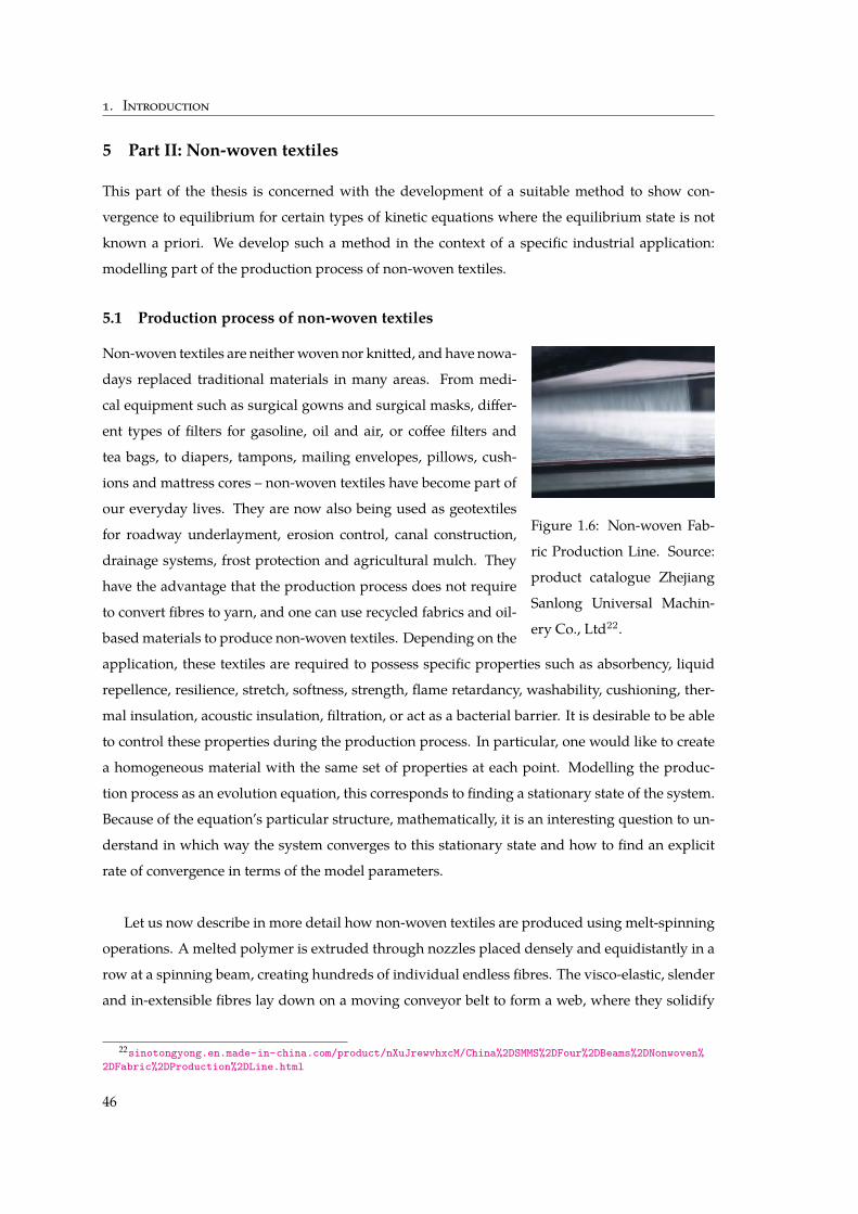
1. Introduction
5 Part II: Non-woven textiles
This part of the thesis is concerned with the development of a suitable method to show con-
vergence to equilibrium for certain types of kinetic equations where the equilibrium state is not
known a priori. We develop such a method in the context of a specific industrial application:
modelling part of the production process of non-woven textiles.
5.1 Production process of non-woven textiles
Figure 1.6: Non-woven Fab-
ric Production Line. Source:
product catalogue Zhejiang
Sanlong Universal Machin-
ery Co., Ltd22.
Non-woven textiles are neitherwoven nor knitted, and have nowa-
days replaced traditional materials in many areas. From medi-
cal equipment such as surgical gowns and surgical masks, differ-
ent types of filters for gasoline, oil and air, or coffee filters and
tea bags, to diapers, tampons, mailing envelopes, pillows, cush-
ions and mattress cores – non-woven textiles have become part of
our everyday lives. They are now also being used as geotextiles
for roadway underlayment, erosion control, canal construction,
drainage systems, frost protection and agricultural mulch. They
have the advantage that the production process does not require
to convert fibres to yarn, and one can use recycled fabrics and oil-
basedmaterials to produce non-woven textiles. Depending on the
application, these textiles are required to possess specific properties such as absorbency, liquid
repellence, resilience, stretch, softness, strength, flame retardancy, washability, cushioning, ther-
mal insulation, acoustic insulation, filtration, or act as a bacterial barrier. It is desirable to be able
to control these properties during the production process. In particular, one would like to create
a homogeneous material with the same set of properties at each point. Modelling the produc-
tion process as an evolution equation, this corresponds to finding a stationary state of the system.
Because of the equation’s particular structure, mathematically, it is an interesting question to un-
derstand in which way the system converges to this stationary state and how to find an explicit
rate of convergence in terms of the model parameters.
Let us now describe in more detail how non-woven textiles are produced using melt-spinning
operations. A melted polymer is extruded through nozzles placed densely and equidistantly in a
row at a spinning beam, creating hundreds of individual endless fibres. The visco-elastic, slender
and in-extensible fibres lay down on a moving conveyor belt to form a web, where they solidify
22sinotongyong.en.made-in-china.com/product/nXuJrewvhxcM/China%2DSMMS%2DFour%2DBeams%2DNonwoven%2DFabric%2DProduction%2DLine.html
46
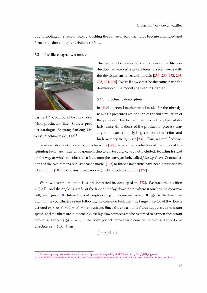
5. Part II: Non-woven textiles
due to cooling air streams. Before touching the conveyor belt, the fibres become entangled and
form loops due to highly turbulent air flow.
5.2 The fibre lay-down model
Figure 1.7: Compound for non-woven
fabric production line. Source: prod-
uct catalogue Zhejiang Sanlong Uni-
versal Machinery Co., Ltd23.
The mathematical description of non-woven textile pro-
duction has received a lot of interest in recent years with
the development of several models [230, 231, 172, 203,
205, 134, 206]. We will now describe the context and the
derivation of the model analysed in Chapter 5.
5.2.1 Stochastic description
In [230] a general mathematical model for the fibre dy-
namics is presented which enables the full simulation of
the process. Due to the huge amount of physical de-
tails, these simulations of the production process usu-
ally require an extremely large computational effort and
high memory storage, see [231]. Thus, a simplified two-
dimensional stochastic model is introduced in [172], where the production of the fibres at the
spinning beam and their entanglement due to air turbulence are not included, focusing instead
on the way in which the fibres distribute onto the conveyor belt, called fibre lay-down. Generalisa-
tions of the two-dimensional stochastic model [172] to three dimensions have been developed by
Klar et al. in [203] and to any dimension N ě 2 by Grothaus et al. in [177].
We now describe the model we are interested in, developed in [172]. We track the position
xptq P R2 and the angle αptq P S1 of the fibre at the lay-down point where it touches the conveyor
belt, see Figure 1.8. Interactions of neighbouring fibres are neglected. If x0ptq is the lay-down
point in the coordinate system following the conveyor belt, then the tangent vector of the fibre is
denoted by τpαptqq with τpαq “ pcosα, sinαq. Since the extrusion of fibres happens at a constant
speed, and the fibres are in-extensible, the lay-down process can be assumed to happen at constant
normalised speed x10ptq “ 1. If the conveyor belt moves with constant normalised speed κ in
direction e1 “ p1, 0q, thendxdt “ τpαq ` κe1.
23sinotongyong.en.made-in-china.com/productimage/HbjmKkDMGOWw-2f1j00kjgTKfpCgYov/China-SMMS-Spunbond-and-Melt-Blown-Compound-Non-Woven-Fabric-Production-Line-Ty-S-Series.html
47
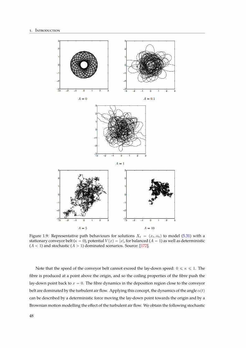
1. Introduction
Figure 1.9: Representative path behaviours for solutions Xt “ pxt, αtq to model (5.31) with astationary conveyor belt (κ “ 0), potential V pxq “ |x|, for balanced (A “ 1) as well as deterministic(A ă 1) and stochastic (A ą 1) dominated scenarios. Source: [172].
Note that the speed of the conveyor belt cannot exceed the lay-down speed: 0 ď κ ď 1. The
fibre is produced at a point above the origin, and so the coiling properties of the fibre push the
lay-down point back to x “ 0. The fibre dynamics in the deposition region close to the conveyor
belt are dominated by the turbulent air flow. Applying this concept, the dynamics of the angleαptq
can be described by a deterministic force moving the lay-down point towards the origin and by a
Brownianmotionmodelling the effect of the turbulent air flow. We obtain the following stochastic
48
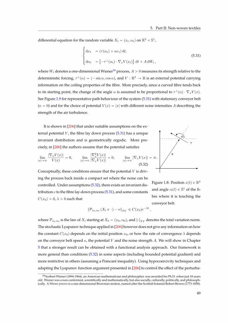
5. Part II: Non-woven textiles
differential equation for the random variable Xt “ pxt, αtq on R2 ˆ S1,$
’
’
&
’
’
%
dxt “ pτpαtq ` κe1qdt,
dαt ““
´τKpαtq ¨∇xV pxtq‰
dt`AdWt ,
(5.31)
whereWt denotes a one-dimensionalWiener24 process,A ą 0 measures its strength relative to the
deterministic forcing, τKpαq “ p´ sinα, cosαq, and V : R2 Ñ R is an external potential carrying
information on the coiling properties of the fibre. More precisely, since a curved fibre tends back
to its starting point, the change of the angle α is assumed to be proportional to τKpαq ¨ ∇xV pxq.
See Figure 1.9 for representative path behaviour of the system (5.31) with stationary conveyor belt
(κ “ 0) and for the choice of potential V pxq “ |x| with different noise intensities A describing the
strength of the air turbulence.
Figure 1.8: Position xptq P R2
and angle αptq P S1 of the fi-
bre where it is touching the
conveyor belt.
It is shown in [206] that under suitable assumptions on the ex-
ternal potential V , the fibre lay down process (5.31) has a unique
invariant distribution and is geometrically ergodic. More pre-
cisely, in [206] the authors assume that the potential satisfies
lim|x|Ñ8
|∇xV pxq|
V pxq“ 0, lim
|x|Ñ8
|∇2xV pxq|
|∇xV pxq|“ 0, lim
|x|Ñ8|∇xV pxq| “ 8.
(5.32)
Conceptually, these conditions ensure that the potential V is driv-
ing the process back inside a compact set where the noise can be
controlled. Under assumptions (5.32), there exists an invariant dis-
tribution ν to the fibre lay-downprocess (5.31), and some constants
Cpx0q ą 0, λ ą 0 such that
Px0,α0 pXt P ¨q ´ νTV ď Cpx0qe´λt ,
where Px0,α0 is the law ofXt starting atX0 “ px0, α0q, and ¨TV denotes the total variation norm.
The stochastic Lyapunov technique applied in [206] however does not give any information on how
the constant Cpx0q depends on the initial position x0, or how the rate of convergence λ depends
on the conveyor belt speed κ, the potential V and the noise strength A. We will show in Chapter
5 that a stronger result can be obtained with a functional analysis approach. Our framework is
more general than conditions (5.32) in some aspects (including bounded potential gradient) and
more restrictive in others (assuming a Poincaré inequality). Using hypocoercivity techniques and
adapting the Lyapunov function argument presented in [206] to control the effect of the perturba-
24NorbertWiener (1894-1964), an Americanmathematician and philosopher, was awarded his Ph.D. when just 18 yearsold. Wienerwas a non-conformist, scientifically andmathematically, but also socially, culturally, politically, and philosoph-ically. AWiener process is a one-dimensional Brownianmotion, named after the Scottish botanist Robert Brown (1773-1858).
49
1. Introduction
tion κBx1 , we prove convergence in a weighted L2-norm and derive an explicit rate of convergence
in terms of κ, D and V .
5.2.2 Kinetic description
As we are not interested in the behaviour of the lay-down point of an individual fibre, but rather
in the distribution of fibres on the belt as the number of fibres is large, we adopt a continuum
description of the stochastic model (5.31). Let us denote by fpt, x, αq the density of the law of
Xt “ pxt, αtq in R2 ˆ S1. Then by Itô’s Lemma25 [266], fpt, x, αq is governed by the linear Fokker–
Planck equation
Btf ` pτ ` κe1q ¨∇xf ´ Bα`
τK ¨∇xV f˘
“ DBααf (5.33)
with diffusivity D “ A22. In other words, fpt, x, αq is the probability density distribution of
fibres touching the belt at point x P R2 at angle α P S1 at time t ě 0.
In Chapter 5, we study the asymptotic behaviour of the kinetic model (5.33) using hypocoercivity
techniques, a framework which we explain in more detail in the next section.
6 Part II: Hypocoercivity
Hypocoercivity is a method to show convergence to equilibrium for dissipative evolution equa-
tions involving a degenerate dissipative operator, and a first order operator generating a time-
reversible conservative equation. Typically, the dissipative part is not coercive, in the sense that
it does not admit a spectral gap. Additionally, its kernel is not stable under the action of the con-
servative part. A strategy to show convergence to equilibrium for this type of equation has been
developed by several groups in the 2000s, see for instance [185, 178, 225, 129? ], and a theoret-
ical framework was adopted by Villani in [298]. The term hypocoercivity26 has been introduced
by Villani by analogy with problems encountered in the theory of hypoellipticity, a concept intro-
duced byHörmander in 1967 [193] and inwhich one is concernedwith regularity issues instead of
convergence to equilibrium. For many important equations, hypoellipticity has been established
around the same time as hypocoercivity through the works of Hérau and Nier [185, 184], Eck-
mann and Hairer [141], Helffer and Nier [182]. However, hypocoercivity and hypoellipticity are
independent concepts, despite the fact that they occur together in a number of models. More pre-
cisely, hypoellipticity can be localised as a property, whereas hypocoercivity cannot as it is always
a global property of the operator.
25Itô’s lemma is occasionally referred to as the Itô–Doeblin Theorem in recognition of posthumously discovered workof Wolfgang Doeblin.
26Hypo is an ancient Greek preposition, which translates as under, whereas hypermeans over or beyond. The term hypoco-ercivity makes allusion to the fact that the operator is ’less than coercive’.
50
6. Part II: Hypocoercivity
As described by Villani himself, the motivation for developing the general hypocoercivity
theory as presented in [298] was 1) to simplify and unify the approach for the results obtained
in [129, 130] for the Fokker–Planck equation and the Boltzmann equation, and 2) to find gen-
eral methods that apply to various models sharing similar features. Villani derives in [298] re-
sults for exponential convergence to equilibrium for rather general operators in an abstract Hör-
mander form and under some commutator assumptions. With this new framework, Villani was
able to prove an abstract and more general version of the non-linear results previously obtained
in [129, 130].
Since the publication of [298], the hypocoercivity approach has been applied in a variety of con-
texts, from micro-magnetism and fluid mechanics (stability of Oseen vortices [162]) to statistical
mechanics (models for propagation of heat [296, 226]). The advantage of the method is that one
can find an explicit rate of convergence to equilibrium. However, this rate is most likely not opti-
mal, and it remains to see if it is quantitatively relevant in the context of the model.
6.1 Abstract hypocoercivity approach: an example
Let us begin with a concrete and simple yet important example to give an idea of the general and
rather abstract hypocoercivity approach. Consider the kinetic Fokker–Planck equation
Btf ` v ¨∇xf “ ∆vf `∇v ¨ pvfq x P TN , v P RN ,
which has normalised stationary stateMpvq :“ p2πq´N2e´|v|2
2 . Since we have omitted the pres-
ence of a confining potential, we work on the torus TN to keep the space variable confined. It is
convenient to formulate the equation for the normalised solution h :“ fM :
Bth` v ¨∇xh “ ∆vh´ v ¨∇vh (6.34)
with stationary state h8 “ 1. Working in the Hilbert space L2pMpvqdxdvq, we denote by@
¨ , ¨D
and || ¨ || the corresponding inner product and norm. Hoping that the operator
L :“ v ¨∇xh´∆vh` v ¨∇vh
may be coercive on H1, one would like to show decay to the equilibrium h8 in the H1-norm
||h||2H1 :“ ||h||2 ` ||∇xh||2 ` ||∇vh||
2. This however is not possible. Taking for example a density
h “ hpxq P L2pMpvqdxdvq that is independent of velocities, we find
12
ddt ||h||
2H1 “
ij
TNˆRN
v ¨∇xh∆xhM dxdv ´ij
TNˆRN
hv ¨∇xhM dxdv
“ ´
ij
TNˆRN
p∆xh´ hq∇x ¨∇vM dxdv “ 0 ,
51
1. Introduction
and so decay cannot be guaranteed once the evolution reaches the set of velocity-independent
densities. Since the null space of the dissipative part´∆v`v ¨∇v is not stable under the transport
part v ¨∇x of the operator, the set of velocity-independent densities is strictly larger than Ker L and
the evolution may not have reached equilibrium yet. The core idea of the hypocoercivity strategy
is to add amixed term@
∇xh , ∇vhD
that can recover the missing decay. Let us define themodified
entropy
Grhs :“ ||h||2 ` a||∇vh||2 ` 2b
@
∇xh , ∇vhD
` c||∇xh||2 (6.35)
with suitable constants c ! b ! a ! 1. Then Gr¨s is norm-equivalent to || ¨ ||H1 as long as b2 ă ac.
However, these two norms are quite different since L is coercive with respect to G, whereas it is
not with respect to || ¨ ||H1 . The reason is the fact that the mixed term@
∇xh , ∇vhD
is able to pick
up the influence of the anti-symmetric part B :“ v ¨∇x of L to recover the derivative in the space
variable:
@
∇xBh , ∇vhD
`@
∇xh , ∇vBhD
“@
B∇xh , ∇vhD
`@
∇xh , ∇vBhD
“@
∇xh , B˚∇vhD
`@
∇xh , ∇vBhD
“ ´@
∇xh , B∇vhD
`@
∇xh , ∇vBhD
“@
∇xh, r∇v , BshD
“ ||∇xh||2 .
Here, we used that ∇x and B commute, anti-symmetry of B, and the fact that r∇v , Bs “ ∇x.
This shows why it may be useful to work with a Hörmander commutator notation similar to Hör-
mander’s hypoellipticity theorem [193]. Let us give the main ideas of a simplified (i.e. only one
commutator instead of several iterated commutators) hypocoercivity statement without going too
much into detail. Following the hypocoercivity formalism established in [298], we write
Btf ` Lf “ 0 , L :“ A˚A` B .
In the example (6.34), we have A :“ p0N ,∇vq and B :“ pv, 0N q ¨∇x,v . Then A˚ “ p0N ,´∇v ´ vq,
and so L can be written in Hörmander form of second type27: L “ ´ř
j A2j ` pB `
ř
j cjAjq with
c :“ p0N , vq. Let us define the commutator C :“ rA,Bs “ AB ´ pB b Id2N qA “ p0N ,∇xq. [298,
Theorem 18]28 states
Theorem 6.1. If B is anti-symmetric, and there exist constants α, β such that
(i) A and A˚ commute with C; A commutes with A (i.e. Ai commutes with Aj for all i, j P t1, . . . , 2Nu;
(ii) rA,A˚s is α-bounded relatively to Id2N ` A;
27In short, this means the operator can be written as sum of squares of derivations, plus a derivation, see [185, 141, 182].28For a detailed description of the commutator notation used here and relative boundedness of operators, see [298].
52
6. Part II: Hypocoercivity
(iii) rB,Cs is β-bounded relatively to A,A2,C and AC;
then there exists a scalar product@@
¨ , ¨DD
on H1K, where K :“ Ker L, that is norm-equivalent to || ¨ ||H1
such that@@
h , LhDD
ě K1`
||Ah||2 ` ||Ch||2˘
for some constantK1 ą 0, only depending on α and β. If, in addition, A˚A`C˚C isK2-coercive for some
K2 ą 0, then there is a constant λ “ λpα, β,K2q ą 0, such that
@h P H1K ,@@
h , LhDD
ě λ@@
h , hDD
.
It follows that L is hypocoercive on fluctuations H1K. It is easy to see that our example (6.34)
satisfies all assumptions of the above theorem. Here,H1K “
!
h P H1 |ť
TNˆRN hMpvqdxdv “ 0)
is the orthogonal of all constant functions@
h8D
in@
¨ , ¨D
, and C “ ∇x. Conditions (i)-(iii) are triv-
ially satisfied since (i) A only acts on velocities, whereas C only acts on space, (ii) rA,A˚s “ Id2N
and (iii) rB,Cs “ 0. Thanks to the Poincaré29 inequality
@h P H1 s.t.ij
TNˆRN
hMpvqdxdv “ 0 : ||∇xh||2 ` ||∇vh||
2 ě K2||h||2 ,
the operator A˚A` C˚C is coercive on H1K. Further,@@
h , hDD
“ Grhs, and so Theorem 6.1 tells
us that there exists a constant λ ą 0 such that
ddtGrhs ď ´2λGrhs . (6.36)
Generally, it is not possible to show ||hptq||H1 ď ||hp0q||H1e´λt as explained above. However, it
follows from norm-equivalence between Gr¨s and || ¨ ||2H1 and from (6.36) that
||hptq||H1 ď c0||hp0q||H1e´λt
on H1K for some λ ą 0 and c0 ą 1. This is exactly what wemean by saying that L is hypocoercive
on H1K.
6.2 Framework for linear kinetic equations
In Chapter 5, we focus on a specific example of a linear kinetic equation conserving mass, a class
of equations for which the general hypocoercivity theory simplifies greatly [135]. For a detailed
account of the general method, see [298, 296] and the references therein. Consider the abstract
ODEddtf ` Tf “ Qf (6.37)
29Jules Henri Poincaré (1854-1912) was a French mathematician, theoretical physicist, engineer, and philosopher ofscience, and often described as a ’polymath’. He was proponent of the view, known as conventionalism, that it is not anobjective question which model of geometry best fits physical space, but is rather a matter of which model we find mostconvenient.
53
1. Introduction
governing the evolution of a density fpt, x, vq, where x and v denote the space and velocity vari-
ables respectively, and fpt, ¨q P H for all t ě 0 for some Hilbert space H. Here, T denotes a
skew-symmetric transport operator and Q is a collision operator that is assumed to be negative
semi-definite. Both operators are possibly unbounded. Further, let us assume that we have exis-
tence of a unique equilibrium distribution F P H of unit mass satisfying TF “ QF . The goal is
to show convergence to F in the norm ¨ corresponding to the Hilbert space H for initial data
fin P H of unit mass.
Hypocoercivity as a method has been developed for equations where the collision part of
the operator only acts on the velocity variable. In particular, denoting by Π the projection onto
velocity-independent densities, Πf :“ ρfF ρF with ρf :“ş
fdv, we have ΠQ “ QΠ “ 0. Since
the mixing only occurs in the velocity variable, it is not directly obvious why one would expect
to observe convergence to equilibrium both in space and in velocity. However, with the good as-
sumptions on T, the mixing in v can be transferred to x via transport effects.
Under the assumptions that T is skew-symmetric and Q is negative semi-definite, one obtains
the H-theorem
ddtf
2 “@
Qf, fD
ď 0 , (6.38)
In other words, ¨ 2 is a Lyapunov functional for equation (6.37). However, this does not give
us any information about the kernel of T. Further, since Q is only negative semi-definite and not
coercive, we cannot directly derive convergence to equilibrium from identity (6.38) as the decay in
¨ 2 pauses as soon as the solution fptq reaches the kernel of Q without necessarily being in the
kernel of T. As described in the previous section, this can be remedied by adding a suitable mixed
term as an equivalent norm, for which the operator is coercive. In this section, we describe how
to formulate the framework of Theorem 6.1 for linear kinetic equations conserving mass without
recourse to commutators, following the functional setting in [135]. The main difference of the
approach taken in [135] compared to [298] is to work in an L2-framework instead of H1, giving
important physical information on the behaviour of solutions. For example, one can obtain ex-
ponential decay even if the initial datum fin oscillates wildly, meaning that the hypocoercivity
method is not sensitive to the regularity of fin. Even though hypoellipticity may provide H1-
regularity, there are two advantages to showing convergence in L2: firstly, the approach in [135]
also applies to equations that are not hypoelliptic, and secondly, an L2-framework is preferable if
one is interested in physical applications and dependence on the initial data. We also point out
that H1-regularisation with global estimates in weighted norms has not been done yet for equa-
tion (6.37). In order to work inL2, definition (6.35) is replacedwith a different generalised entropy
using a suitable auxiliary operator.
54
6. Part II: Hypocoercivity
6.2.1 Generalised entropy
The main idea of the convergence proof for hypocoercive operators is to find a Lyapunov func-
tional, a generalised entropy, that is better than the ’natural’ entropy ¨ 2, by adding carefully cho-
sen lower-order terms. This approach is motivated by [184] in the context of commutator theory
for hypoelliptic operators, see Section 6.1. In the case of a linear kinetic equation of type (6.37), a
suitable generalised entropy G : H Ñ R` is given by
Grf s :“ 12f
2 ` ε@
Af, fD
, ε ą 0
with
A :“ p1` pTΠq˚TΠq´1pTΠq˚ . (6.39)
The ˚-notation refers to the adjoint in the inner product@
¨, ¨D
corresponding to H. Note that
pTΠq˚TΠ is an elliptic operator. The operator A is bounded and regularises the solution to (6.37)
in the space variable (and it is not the same as the operator A in Section 6.1). The idea of choosing
this generalised entropy is due to [135] and allows to use the projection Π instead of having to
deal with ∇v . Here, pTΠq˚ plays the role of the mixed term@
∇xh , ∇vhD
in (6.35), and choosing
A “ pTΠq˚ would be enough to build a hypocoercivity theory along the lines of Theorem 6.1. The
main idea of choosing A as in (6.39) is borrowed from Hérau [184]: replacing the H1-norm plus
a mixed term with a mixed term only, but which is divided by a second order operator to obtain
an operator of order zero (i.e. no derivatives). Here, the operator A is of order ´1, but allows to
show that solutions to (6.37) decay exponentially fast in L2, i.e. the aim is to find an explicit λ ą 0
such that ddtG ď ´λG and show that G is norm-equivalent to || ¨ ||2.
6.2.2 Microscopic and macroscopic coercivity
Let us differentiate G along trajectories of the system,
ddtGrf s “
@
Qf, fD
´ ε@
ATΠf, fD
´ ε@
ATp1´ Πqf, fD
` ε@
TAf, fD
` ε@
AQf, fD
, (6.40)
using the fact that T is skew-symmetric, and so@
Tf, fD
“ 0, as well as QA “ 0 which follows since
g :“ Af satisfies g “ ´ΠTf `ΠT2Πg and so it is in the kernel of Q. The first term can be conrolled
by the following microscopic coercivity assumption: there exists λm ą 0 such that
´@
Qf, fD
ě λmp1´ Πqf2 . (6.41)
In other words, this means that we require the collision operator Q to be coercive on the comple-
ment of its kernel. In order to control the second term in (6.40), we need that the elliptic operator
ATΠ satisfies a Poincaré inequality, which corresponds to a spectral gap on the macroscopic level.
This can be formulated as the following macroscopic coercivity assumption: there exists λM ą 0
55
1. Introduction
such that
TΠf2 ě λM Πf2 ùñ@
ATΠf, fD
ěλM
1` λMΠf2 . (6.42)
In other words, the restriction of T to Ker Q is coercive.
6.2.3 Diffusive macroscopic limit
Take a change of variables pt, x, vq ÞÑ ptε2, xε, vq in equation (6.37) depending on 0 ă ε ! 1 such
that the rescaled density fεpt, x, vq “ f`
tε2, xε, v˘
satisfies
ε2 ddtf
ε ` εTfε “ Qfε . (6.43)
Consider fluctuations around the set of velocity-independent densities, that is fε “ Πfε` εRε for
some Rε P H. Substituting this ansatz into (6.43) and projecting onto the kernel of Q, we obtain
the conservation law
εddt pΠf
εq ` ΠTΠfε ` εΠTRε “ 0 , (6.44)
since Π2 “ Π, ΠRε “ Πp1´ Πqfεε “ 0 and ΠQ “ 0. Assuming that fε Ñ f0 and Rε Ñ R0 in the
limit εÑ 0, we obtain the identity
ΠTΠ “ 0 . (6.45)
It follows from (6.43) that Qf0 “ 0, and since f0 is in KerQ, we conclude that f0 “ Πf0. Further,
dividing (6.43) by ε and using that QΠ “ 0, we have
εddtf
ε ` Tfε “ Qfεε “ Qp1´ Πqfεε “ QRε .
Therefore, we obtain in the limit that Tf0 “ QR0. Recalling that f0 “ Πf0, we have
R0 “ Q´1Tf0 “ Q´1TΠf0 , Q :“ Q|p1´ΠqH .
Finally, dividing (6.44) by ε and using (6.45), we obtain in the limit εÑ 0 themacroscopic equation
BtΠf0 ´ pTΠq˚ Q´1TΠf0 “ 0 ,
where we used that T is skew-symmetric T˚ “ ´T, and Π˚ “ Π. In other words, assuming
ΠTΠ “ 0 corresponds to a diffusive macroscopic limit of equation (6.37).
6.2.4 Exponential convergence
The price to pay by using the generalised entropy G is that one needs to be able to control the last
three terms in (6.40) also. The assumption ΠTΠ “ 0 yields [135, Lemma 1]
Af ď 12p1´ Πqf , TAf ď p1´ Πqf .
56
7. Part II: Results
It follows from the first estimate that G is norm-equivalent to the Hilbert space norm ¨ 2 if ε ă 1.
Finally, it remains to show that the following auxiliary operators are bounded:
@
ATp1´ Πqf, fD
`@
AQf, fD
ď CM p1´ Πqf2 (6.46)
for some constant CM ą 0. Putting all the bounds together, we obtain exponential decay of fptq,
i.e. hypocoercivity, with an explicitly computable rate depending on λm, λM , CM , assuming that
(6.41), (6.42), (6.46) and ΠTΠ “ 0 hold. For the detailed proof of this statement, see [135].
Applications of the hypocoercivity approach in the linear kinetic setting include equations con-
taining confinement terms and different types of collision operators with mass conservation, such
as the Fokker–Planck equation, scattering models and the linearised BGK equations, see [135] and
the references therein. Further recent applications include the fibre-lay down process (5.33) for a
stationary conveyor belt [134], a velocity-jump model for bacterial chemotaxis [69], and particles
interacting with a vibrating medium [1].
7 Part II: Results
In Chapter 5, we apply the hypocoercivity method described above to the linear kinetic equation
modelling the fibre lay-down in the production process of non-woven textiles as formulated in
(5.33). The full hypocoercivity analysis of the long-time behaviour of solutions to this kinetic
model in the case of a stationary conveyor belt κ “ 0 is completed in [134]. In the case κ “ 0, there
exists a unique global normalised equilibrium distribution
F0pxq “e´V pxq
ş
R2 eV pxqdx.
For technical applications in the production process of non-wovens, one is interested in a model
including the movement of the conveyor belt, and in Chapter 5, we extend the results in [134] to
the case κ ą 0. This is not a trivial task for several reasons. First of all, for a moving conveyor belt,
we are not able to find a stationary state for equation (5.33) explicitly. The hypocoercivity method
however is used to find estimates about rates of convergence after the existence and uniqueness of
a steady state have been established.
Secondly, adding the movement of the belt breaks the symmetry of the problem, and the operator
assumptions required for the hypocoercivity strategy to work do not hold in the ’natural’ func-
tional framework. However, the hypocoercivity theory is based on a priori estimates [135], and is
therefore stable under perturbation. Wewill show in Chapter 5 how the hypocoercivity technique
can be adapted to this context under the assumption that the conveyor belt moves slow enough.
57
1. Introduction
7.1 Functional framework
To set up a suitable functional framework for the fibre lay-down process, we rewrite the Fokker–
Planck equation (5.33) as an abstract ODE
Btf “ Lκf “ pQ´ Tq f ` Pκf, (7.47)
where Q :“ DBαα represents collisions, Pκ is the perturbation introduced by the moving belt,
Pκf :“ ´κe1 ¨∇xf,
and the transport operator T is given by
Tf :“ τ ¨∇xf ´ Bα`
τK ¨∇xV f˘
.
The main idea here is to introduce a weight function g that allows the control of the perturbative
term in the case when the potential gradient ∇xV is unbounded:
gpx, αq “ expˆ
βV pxq ` |∇xV pxq|Γˆ
τpαq ¨∇xV pxq
|∇xV pxq|
˙˙
if |∇xV | Ñ 8 as |x| Ñ 8, and g ” 0 otherwise. For a detailed definition of β ą 1 and Γ P
C1 pr´1, 1sq, Γ ą 0, see Chapter 5 Section 3. We consider solutions to (7.47) in the spaceL2pdµκq :“
L2pR2 ˆ S1,dµκqwith measure
dµκpx, αq “´
eV pxq ` ζκgpx, αq¯ dxdα
2π .
We denote by x¨, ¨yκ the corresponding scalar product and by ¨ κ the associated norm. Here,
ζ ą 0 is a free parameter that needs to be chosen big enough depending on the relative speed of
the conveyor belt κ in order to guarantee convergence to equilibrium.
In this functional setting, the operators T, Q and Pκ have several nice properties that allow us
to apply the general hypocoercivity theory for linear kinetic equations conserving mass as out-
lined in [135]. First of all, if κ “ 0, then Q and T are closed operators on L2pdµ0q such that Q´ T
generates the C0-semigroup epQ´Tqt on L2pdµ0q [134]. Adding the movement of the belt (κ ą 0),
we use the additional weight function g ą 0 to control the perturbative term Pκ in the case of
unbounded potential gradients. This allows us to construct a C0-semigroup for Lκ “ Q´ T` Pκalso for κ ą 0 (Theorem 4.1 in Chapter 5). Note that Lκ is closable in L2pdµκq and its operator core
is given by C :“ C8c`
R2 ˆ S1˘. Unless otherwise specified, all computations are performed on C,
and can be extended to L2pdµκq by density arguments.
The orthogonal projection Π on the set of local equilibria KerQ is Πf :“ 12π
ş
S1 f dα, and we define
the mass of a given distribution f P L2pdµκq byMf “ş
R2 Πf dx. Integrating (7.47) over R2 ˆ S1,
we see that the mass of any solution of (7.47) is conserved over time. Moreover, any solution of
58
7. Part II: Results
(7.47) remains non-negative as soon as the initial datum is non-negative.
In the case of a stationary conveyor belt κ “ 0, it was shown in [134] that the fibre lay-down
model (7.47) fits into the hypocoercivity theory of linear kinetic equations conserving mass de-
scribed in Section 6.2. Indeed, the collision operator Q is symmetric and negative semi-definite on
C,
xQf, fy0 “ ´D Bαf20 ď 0 ,
i.e. Q is dissipative in L2pdµ0q. Further, we have TΠf “ e´V τ ¨∇xuf for f P C with uf :“ eV Πf ,
which implies ΠTΠ “ 0 on C. Our approach for tackling the problem of exponential convergence
if κ ą 0 is to treat the system as a small perturbation of the case κ “ 0 for which microscopic and
macroscopic coercivity are satisfied for sufficiently ’nice’ potentials V .
In order to ensure that the operators Q and T satisfy microscopic and macroscopic coercivity
respectively, we need to impose certain assumptions on the external potential V . Further, in order
to recover convergence to equilibrium for the perturbed equation κ ą 0, we need to make sure
that the perturbation Pκ can be controlled in a suitable way. Therefore, we make the following
assumptions on the external potential V :
(H1) Regularity and symmetry: V P C2pR2q and V is spherically symmetric outside some ball
Bp0, RV q.
(H2) Normalisation:ş
R2 e´V pxq dx “ 1.
(H3) Spectral gap condition: there exists a positive constant Λ such that for any u P H1pe´V dxq
withş
R2 ue´V dx “ 0, we have the Poincaré inequality
ż
R2|∇xu|
2e´V dx ě Λ
ż
R2u2e´V dx.
(H4) Pointwise condition: there exists c1 ą 0 such that for any x P R2,
|∇2xV pxq| ď c1p1` |∇xV pxq|q,
where ∇2xV denotes the Hessian of V pxq.
(H5) Behaviour at infinity:
lim|x|Ñ8
|∇xV pxq|
V pxq“ 0, lim
|x|Ñ8
|∇2xV pxq|
|∇xV pxq|“ 0 .
Assumptions (H2-3-4) are as stated in [134]. Assumption (H1) assumes regularity of the potential
that is stronger and included in that discussed in [134] since (H1) implies V PW 2,8loc pR
2q. Roughly
speaking, (H2) and (H3) require a sufficiently strong growth of V pxq at infinity, whereas (H4) puts
59
1. Introduction
a limitation on the growth behaviour. This leaves room, however, for a large class of confining
potentials including V pxq “ p1 ` |x|2qs2, s ě 1. Assumption (H5) is only necessary if the poten-
tial gradient |∇xV | is unbounded. Both bounded and unbounded potential gradients may appear
depending on the physical context.
Thanks to the spectral gap condition (H3), microscopic and macroscopic coercivity follow:
• Microscopic coercivity: The operator Q is symmetric and the Poincaré inequality on S1,
12π
ż
S1|Bαf |
2 dα ě 12π
ż
S1
ˆ
f ´1
2π
ż
S1f dα
˙2dα,
yields that for all f in the operator domain DpQq,
´xQf, fy0 ě D p1´ Πqf20 .
• Macroscopic coercivity: The operator T is skew-symmetric and for any h P L2pdµq such that
uh “ eV Πh P H1pe´V dxq andť
R2ˆS1 hdµ “ 0, we have
TΠh20 “1
4π
ij
R2ˆS1
e´V |∇xuh|2 dx dα
ěΛ4π
ij
R2ˆS1
e´V u2h dxdα “ Λ
2 Πh20
by the spectral gap condition (H3).
Inspired by [135], we define the hypocoercivity functional
Grf s :“ 12f
2κ ` ε1xAf, fy0 ,
with the auxiliary operator A as given in (6.39), and for some suitably chosen ε1 P p0, 1q to be
determined later. It follows from [135] that Gr¨s is equivalent to ¨ 2κ on L2pdµκq,ˆ
1´ ε1
2
˙
f2κ ď Grf s ďˆ
1` ε1
2
˙
f2κ ,
7.2 Hypocoercivity estimate and convergence
In Chapter 5, we prove a hypocoercivity estimate on the dissipation of the generalised entropy
G that allows us to deduce both existence and uniqueness of an equilibrium distribution Fκ to
equation (7.47) in the case of a moving conveyor belt κ ą 0. Let us emphasize that a specific
contribution of this work is to introduce two (and not one as in [135, 134]) modifications of the
entropy: 1) we first modify the space itself with the coercivity weight g, then 2) we change the
norm with an auxiliary operator following the hypocoercivity approach. As opposed to [134],
where the authors estimate dGdt on fluctuations around the equilibrium F0 for κ “ 0, we derive
a more general estimate for any f P L2 pdµκq, involving an additional mass term:
60
7. Part II: Results
Proposition 7.1. Assume that hypothesis (H1-2-3-4-5) hold and that 0 ă κ ă 1 is small enough (with a
quantitative estimate). Let fin P L2pdµκq and f “ fpt, x, αq be a solution of (5.33) in L2pdµκq subject to
the initial condition fpt “ 0q “ fin. Then f satisfies the following Grönwall type estimate:
ddtGrfpt, ¨qs ď ´γ1Grfpt, ¨qs ` γ2M
2f , (7.48)
where γ1 ą 0, γ2 ą 0 are explicit constants only depending on κ, D and V .
Estimate (7.48) allows us to establish existence of solutions to (7.47) using semigroup theory
(Theorem 4.1 in Chapter 5). More importantly, the above hypocoercivity estimate is the key in-
gredient that ensures existence and uniqueness of an equilibrium distribution Fk P L2 pdµκq for
equation (7.47). The main idea of the existence proof is to seek a stationary state in the bounded
set
B :“"
f P L2pdµκq : Grf s ď γ2
γ1, f ě 0, Mf “ 1
*
using a contraction argument. More precisely, we show in Chapter 5 Section 4.2 that the set B is
preserved under the action of the semi-group: StpBq Ă B for all t ě 0. Together with the hypoco-
ercivity estimate (7.48) and Banach’s fixed point theorem, this allows us to find ut P B such that
Stputq “ ut for all t ě 0. Further, proving that B is sequentially compact and repeatedly apply-
ing the semi-group property of St, we show that there exists u P B independent of t such that
Stpuq “ u for all t ě 0. This concludes the existence of a stationary state Fk of unit mass for
equation (7.47). Moreover, when applied to the difference of two solutions with the same mass,
the hypocoercivity estimate (7.48) gives an estimate on the exponential decay rate towards equi-
librium, and so uniqueness follows.
Our results in Chapter 5 can be summarised by the following theorem:
Theorem 7.2. Let fin P L2pdµκq and let (H1-2-3-4-5) hold. For 0 ă κ ă 1 small enough (with a
quantitative estimate) and ζ ą 0 large enough (with a quantitative estimate), there exists a unique non-
negative stationary state Fκ P L2pdµκq with unit massMFκ “ 1. In addition, for any solution f of (5.33)
in L2pdµκq with massMf and subject to the initial condition fpt “ 0q “ fin, we have
fpt, ¨q ´MfFκκ ď C fin ´MfFκκ e´λκt ,
where the rate of convergence λκ ą 0 depends only on κ, D and V , and the constant C ą 0 depends only
on D and V .
61
1. Introduction
In the case of a stationary conveyor belt κ “ 0 considered in [134], the stationary state is char-
acterised by the eigenpair pΛ0, F0q with Λ0 “ 0, F0 “ e´V , and so Ker L0 “ xF0y. This means that
there is an isolated eigenvalue Λ0 “ 0 and a spectral gap of size at least r´λ0, 0s with the rest of
the spectrum ΣpL0q to the left of´λ0 in the complex plane. Adding the movement of the conveyor
belt, Theorem 7.2 shows that Ker Lκ “ xFκy and the exponential decay to equilibrium with rate
λκ corresponds to a spectral gap of size at least r´λκ, 0s. Further, it allows to recover an explicit
expression for the rate of convergence λ0 for κ “ 0. In general, we are not able to compute the
stationary state Fκ for κ ą 0 explicitly, but Fκ converges to F0 “ e´V weakly as κÑ 0.
Remark 7.3. Let us compare our assumptions (H1-2-3-4-5)with the conditions the authors require in [206]
to show a stochastic convergence result in the case of a perturbed process (κ ą 0). Our framework (H1-
2-3-4-5) is more general than conditions (1.4) in some aspects (including bounded potential gradient) and
more restrictive in others (assuming a Poincaré inequality). The proof in [206] relies on the strong Feller
property which can be translated in some cases into a spectral gap; it also uses hypoellipticity to deduce
the existence of a transition density, and concludes via an explicit Lyapunov function argument. With our
framework (H1-2-3-4-5), and adapting the Lyapunov function argument presented in [206] to control the
effect of κBx1 , we derive an explicit rate of convergence in terms of κ, D and V .
7.3 Perspectives
Working in L2pdµκq Ă L2pdµ0qwe are treating the operator Lκ as a small perturbation of the case
κ “ 0 with stationary conveyor belt. The natural space to investigate the convergence to Fκ in the
case κ ą 0 however is L2 `F´1κ dx dα
˘
. In this L2-space the transport operator T´ Pκ is not skew-
symmetric and the collision operator Q is not self-adjoint, so the hypocoercivity method [135]
cannot be applied. To get around this, one can split the operator Lκ differently into a transport
and a collision part following the approach in [69]. More precisely, we can write Lκ “ Q ´ T
where$
’
’
&
’
’
%
Qf “ Bα´
DBαf ´BαFκFκ
f¯
,
Tf “ pτ ` κe1q ¨∇xf ´ Bα“`
τK ¨∇xV `BαFκFκ
˘
f‰
.
Then in L2 `F´1κ dxdα
˘
the operator Q is symmetric and negative semi-definite, and the operator
T is skew-symmetric. Furthermore, the stationary state Fκ lies in the intersection of the kernels
of the collision and transport operators, i.e. Fκ P Ker Q X Ker T. The hypocoercivity approach
requires microscopic and macroscopic coercivity of Q and T. To this end, we need to be able to
control the behaviour of the stationary state at infinity as in [69], i.e. for large enough |x|,
@α P S1, e´σ1V pxq ď Fκpx, αq ď e´σ2V pxq
for some constants σ1, σ2 ą 0. If true, this would be an important physical information on the
stationary state, but we still do not know how to prove it. Even with this information at hand,
62
7. Part II: Results
this approach requires that the existence of the stationary state be known a priori. The rate of
convergence one obtains in this case may be different from the rate obtained here, and it is not
clear which method yields the better rate as both are most likely not optimal.
There are several ways in which one could seek to improve the results in Chapter 5. For exam-
ple, one could try to push the convergence result to larger values of κ using bifurcation techniques.
More precisely, for a path p : κ ÞÑ Fk mapping κ to the stationary state Fκ of equation (5.33), The-
orem (7.2) guarantees that p is defined on a small interval r0, κ0q for some 0 ă κ0 ! 1. It may be
possible to extend this interval by showing that the implicit equation P pκ, Fκq “ 0 defining the
stationary state Fκ is non-degenerate, i.e. that B2P pκ, Fκq ‰ 0.
Another future avenue would be to apply the techniques developed here to other models where
the global equilibrium is not known a priori.
63
1. Introduction
8 Part III: From micro to macro
The 6th problem asked by Hilbert30 in 1900 is concerned with the axiomatisation of physics. More
than 100 years later it is still unresolved, andmight never be considered completed as the problem
statement is rather broad. Precisely, the original German textMathematische Probleme states:
Durch die Untersuchungen über die Grundlagen der Geometrie wird uns die Auf-
gabe nahegelegt, nach diesemVorbilde diejenigen physikalischen Disciplinen axioma-
tisch zu behandeln, in denen schon heute die Mathematik eine hervorragende Rolle
spielt; dies sind in erster Linie die Wahrscheinlichkeitsrechnung und die Mechanik.
Was die Axiome der Wahrscheinlichkeitsrechnung31 angeht, so scheint es mir wün-
schenswert, daß mit der logischen Untersuchung derselben zugleich eine strenge und
befriedigende Entwickelung der Methode der mittleren Werte in der mathematischen
Physik, speziell in der kinetischen Gastheorie Hand in Hand gehe.
Ueber die Grundlagen der Mechanik liegen von physikalischer Seite bedeutende Un-
tersuchungen vor; ich weise hin auf die Schriften von Mach32, Hertz33, Boltzmann34
und Volkmann35; es ist daher sehr wünschenswert, wenn auch von den Mathematik-
ern die Erörterung der Grundlagen der Mechanik aufgenommen würde. So regt uns
beispielsweise das Boltzmannsche Buch über die Principe der Mechanik an, die dort
angedeuteten Grenzprocesse, die von der atomistischen Auffassung zu den Gesetzen
über die Bewegung der Continua führen, streng mathematisch zu begründen und
durchzuführen. Umgekehrt könnte man die Bewegung über die Gesetze starrer Kör-
per durch Grenzprocesse aus einem System von Axiomen abzuleiten suchen, die auf
der Vorstellung von stetig veränderlichen, durch Parameter zu definirenden Zustän-
den eines den ganzen Raum stetig erfüllenden Stoffes beruhen - ist doch die Frage nach
der Gleichberechtigung verschiedener Axiomensysteme stets von hohemprincipiellen
Interesse.
The problem, suggested by Boltzmann’s work on the principles of mechanics [45], is therefore to
develop “mathematically the limiting processes [...] which lead from the atomistic view to the
laws of motion of continua”, namely to obtain a unified description of gases, including all levels
30David Hilbert (1862-1943) was a German mathematician and is recognised as one of the most influential and uni-versal mathematicians of the 19th and early 20th centuries. He was invited to address the 2nd International Congress ofMathematicians in Paris in 1900, where he proposed 23 problems that are known today as Hilbert’s problems.
31Vgl. Bohlmann, Ueber Versicherungsmathematik 2te Vorlesung aus Klein und Riecke, Ueber angewandte Mathe-matik und Physik, Leipzig und Berlin 1900
32Die Mechanik in ihrer Entwickelung, Leipzig, zweite Auflage. Leipzig 188933Die Principien der Mechanik, Leipzig 189434Vorlesungen über die Principien der Mechanik, Leipzig 189735Einführung in das Studium der theoretischen Physik, Leipzig 1900
64
8. Part III: From micro to macro
of description. In other words, the challenging question is whether macroscopic concepts can be
understood microscopically.
The set of methods for making the connection between microscopic and macroscopic models are
called multiscale analysis or scaling process or limiting process. The idea of multiscale analysis is to
mathematically derive one particularmodel describingmacroscopic phenomena in the observable
physical world, from a microscopic model that is based on interactions between atoms, particles,
or agents. Typically, the microscopic model (depending on space, time and velocity) contains
more information than the macroscopic one (depending only on space and time). One can make
the connection between these two regimes by averaging over the velocities and rescaling the time
and space variables. Mathematically, this corresponds to ’zooming out’, and sowe are exchanging
the loss of information on the kinetics with the ability to capture emerging dynamics of the bulk of
particles that were only implicit in the kinetic equation. The choice of rescaling influences which
phenomenawe are able to observe on themacroscopic scale and has to be chosen in a sensible way
to match the physical context: if we speed up time too much with respect to the scaling in space,
the particles may escape to infinity andwe see nothing; if we do not speed up time fast enough, no
change will occur on the macroscopic level and so no interesting phenomena arise. Since certain
information are lost in the scaling process, it is possible that different kinetic models lead to the
same macroscopic equation. Examples of limiting processes for kinetic equations can be found in
the classical references [263, 103, 294]. Let us mention that the terms ’microscopic’, ’macroscopic’
and ’mesoscopic’ are sometimes used ambiguously in the literature. In this thesis, wewill use ’mi-
croscopic’ in the sense of ’kinetic’ as opposed to a regime describing individual particle dynamics.
Building on the ideas of Maxwell in [232], in 1872, Boltzmann published his famous work [46]
on what can be considered the master equation of kinetic theory
Btf ` v ¨∇xf “ Qpf, fq , (8.49)
where x P RN represents position and v P RN velocity, for the probability density fpt, x, vq. The
bilinear collision operator Q may differ depending on the type of microscopic interactions at play.
Equation (8.49) is known as the Boltzmann equation andwas derived for a monoatomic rarefied gas
by merging mechanical concepts and statistical considerations [232, 46]. It describes gas particles
undergoing free transport and collisions. In the modern literature, the term Boltzmann equation
is often used in a more general sense, referring to any kinetic equation that describes the change
of some quantity such as energy, charge or particle number in a thermodynamic system.
Chapter 6 is centred around the idea of understanding the relationship between different ki-
netic and macroscopic models using multiscale analysis. Diffusion approximations to kinetic
65
1. Introduction
equations have been studied in various works, see for example [293, 13, 26, 121, 210, 258] and
the references therein. In this section, we discuss two particular scaling approaches that play a
role in Chapter 6, grazing collision limits and parabolic diffusion limits, exemplified by the Boltz-
mann equation (8.49) for different choices of collision kernels Q. The latter shows how a limiting
process can be used to derive the classical Keller–Segel model (1.1) from a kinetic description for
bacterial motion.
8.1 The Boltzmann equation: grazing collisions
The Boltzmann equation (8.49) has generated over the past century (and is still generating) a vast
volume of literature, see [294] and the references therein. The Boltzmann collision kernel Q is
given in its general form by
Qpf, fq “ż
R3
ż
S2Bpv ´ v˚, θqpf
1f 1˚ ´ ff˚q dσdv˚ ,
where v and v˚ are the pre-collisional velocities that determine the post-collisional velocities v1
and v1˚ respecting conservation of energy and momentum, parametrised by the unit vector σ:
v1 “v ` v˚
2 `|v ´ v˚|
2 σ ,
v1˚ “v ` v˚
2 ´|v ´ v˚|
2 σ .
For brevity, we write f 1˚ “ fpt, x, v1˚q etc. The deflection angle θ P r0, π2s is such that cos θ “
pv ´ v˚q ¨ σ|v ´ v˚|. The kernel B is determined depending on the nature of interaction between
particles. We will here only concentrate on one particular type of particle interaction that is rel-
evant for the analysis in Chapter 6: If we assume that particles interact through a 1rs force law,
where r is the distance between interacting particles, then the kernel B has a non-integrable sin-
gularity at θ “ 0 which corresponds to grazing collisions. Grazing collisions are collisions that do
not deviate the particles too much. In many studies, the singularity issue is avoided by replacing
B with a locally integrable collision kernel, which is usually referred to as cut-off process [175].
But what happens if there are more and more collisions, but these collisions generate smaller and
smaller deviations? This limit process is known as grazing collision limit.
It is known that in the limit and under certain assumptions, solutions of the Boltzmann equation
(8.49) converge to solutions of the Fokker-Planck-Landau (FPL) equation [158, 157]. The FPL equa-
tion describes the binary collisions between charged particles occurring in a plasma [128, 219] and
was introduced as an approximation of the Boltzmann equation (8.49) in the case of Coulomb in-
teractions [208]. In fact, the Boltzmann operatorQpf, fq ismeaningless in the case of a Coulomb in-
teraction as the effect of grazing collisions prevails over the effect of other collisions in that case. In
the early 90’s, Degond and Lucquin-Desreux [122] and Desvillettes [127] showed the convergence
66
8. Part III: From micro to macro
of the Boltzmann operator Q to the FPL operator (not to be confused with convergence of the solu-
tions). For further results clarifying the connection between the Boltzmann equation and the FPL
equation, see [291, 158]. For more details on the grazing collision limit, see [8, 122, 127, 291, 292]
and the references therein. In Chapter 6, we will use a grazing collision limit to derive a Vlasov-
type flocking equation from a kinetic model for collective animal behaviour. The kinetic model
is of Boltzmann-type in the sense that the collision kernel describing the interaction between two
colliding gas particles is replacedwith an interaction kernel describing the communicationmecha-
nism between individuals. Albeit very different applications, the general structures of these equa-
tions are similar. Applying a grazing limit to this Boltzmann-type equation, we obtain a flocking
model that has been previously derived from individual-based models (Vicsek or Cucker-Smale
models), see Chapter 6 Section 3.2.
8.2 Bacterial chemotaxis: a kinetic description
Boltzmann’s idea for modelling the dynamics of a rarefied monoatomic gas can be transferred to
a wide range of applications using kinetic equations of a similar structure. In the context of this
thesis, it is noteworthy that a non-linear generalisation of the classical Keller–Segel model (1.1)
can, in fact, be derived from a kinetic Boltzmann-type equation via multiscale analysis. Or, to be
more precise, by making the connection to the underlying microscopic dynamics that drive the
emerging patterns on the macroscopic level, we can understand better why certain limitations of
the classical Keller–Segel model arise. In fact, the classical Keller–Segel model does not take the
microscopic scale into account and it is an oversimplified description of the real dynamics as can
be seen by the dramatic blow-up in the two dimensional case [136]. Starting with a microscopic
description of the movement of a single cell in response to chemical gradients, one can use a diffu-
sive limiting process to derive a macroscopic model for bacterial chemotaxis. Wewill here explain
this scaling in more detail since it provides the mathematical tools for performing the multiscale
analysis of a two-dimensional kinetic models for social interactions studied in Chapter 6.
Let us consider a model for bacterial chemotaxis, where the first equation in (1.1) (macroscopic
evolution of the cell density) is replaced by a kinetic equation, whilst the chemoattractant concen-
tration Spt, xq is still governed by the macroscopic diffusion equation
BtS “ DS∆S ´ αS ` βρ . (8.50)
where ρpt, xq “ş
vεVfpt, x, vqdv denotes the macroscopic cell density. Here, α ě 0 and β ě 0 are
the degradation and production rates of the chemoattractant respectively.
67
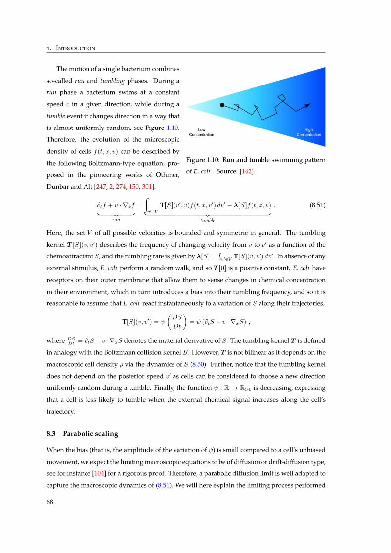
1. Introduction
Figure 1.10: Run and tumble swimming pattern
of E. coli . Source: [142].
The motion of a single bacterium combines
so-called run and tumbling phases. During a
run phase a bacterium swims at a constant
speed c in a given direction, while during a
tumble event it changes direction in a way that
is almost uniformly random, see Figure 1.10.
Therefore, the evolution of the microscopic
density of cells fpt, x, vq can be described by
the following Boltzmann-type equation, pro-
posed in the pioneering works of Othmer,
Dunbar and Alt [247, 2, 274, 150, 301]:
Btf ` v ¨∇xflooooooomooooooon
run
“
ż
v1PV
TrSspv1, vqfpt, x, v1q dv1 ´ λrSsfpt, x, vqlooooooooooooooooooooooooooooomooooooooooooooooooooooooooooon
tumble
. (8.51)
Here, the set V of all possible velocities is bounded and symmetric in general. The tumbling
kernel T rSspv, v1q describes the frequency of changing velocity from v to v1 as a function of the
chemoattractant S, and the tumbling rate is given byλrSs “ş
v1PVTrSspv, v1q dv1. In absence of any
external stimulus, E. coli perform a random walk, and so T r0s is a positive constant. E. coli have
receptors on their outer membrane that allow them to sense changes in chemical concentration
in their environment, which in turn introduces a bias into their tumbling frequency, and so it is
reasonable to assume that E. coli react instantaneously to a variation of S along their trajectories,
TrSspv, v1q “ ψ
ˆ
DS
Dt
˙
“ ψ pBtS ` v ¨∇xSq ,
where DSDt “ BtS` v ¨∇xS denotes the material derivative of S. The tumbling kernel T is defined
in analogy with the Boltzmann collision kernel B. However, T is not bilinear as it depends on the
macroscopic cell density ρ via the dynamics of S (8.50). Further, notice that the tumbling kernel
does not depend on the posterior speed v1 as cells can be considered to choose a new direction
uniformly random during a tumble. Finally, the function ψ : R Ñ Rą0 is decreasing, expressing
that a cell is less likely to tumble when the external chemical signal increases along the cell’s
trajectory.
8.3 Parabolic scaling
When the bias (that is, the amplitude of the variation of ψ) is small compared to a cell’s unbiased
movement, we expect the limitingmacroscopic equations to be of diffusion or drift-diffusion type,
see for instance [104] for a rigorous proof. Therefore, a parabolic diffusion limit is well adapted to
capture the macroscopic dynamics of (8.51). We will here explain the limiting process performed
68
8. Part III: From micro to macro
in [265] that allows to recover the classical Keller–Segel model for the fully coupled system.
The key assumption allowing to pass to a macroscopic description is that the turning proba-
bility TrSspv, v1q is a small perturbation of a random turning process,
TrSspv, v1q “ ψ0 ` εψ0φrSspvq , ε ! 1 ,
where the signal response function φ is to be chosen according to the reaction of cells to the
stimulus S. Rescaling the kinetic equation to its non-dimensional form, and changing variables
pt, x, vq ÞÑ ptε2, xε, vq, we obtain the following equation for the rescaled density fεpt, x, vq in the
new variables:
εBtfε ` v ¨∇xf “
µ
ε
´
ρεpt, xq ´ |V |fεpt, x, vq¯
`
µ
„ż
v1εV
φrSεspv1qfεpt, x, v1qdv1 ´ |V |φrSεspvqfεpt, x, vq
,(8.52)
where ρεpt, xq “ş
vεVfεpt, x, vqdv denotes themacroscopic cell density, andµ is a non-dimensional
coefficient of order 1. Taking the limit ε Ñ 0, and assuming that fε, ρε, Sε converge to f0, ρ0, S0
respectively, the dominant term is a relaxation towards a uniform distribution in velocity at each
position: f0pt, x, vq “ ρ0pt, xq|V |. Integrating (8.52) over V , we obtain
Btρε `∇ . jε “ 0, jε :“ 1
ε
ż
vεV
vfεpt, x, vqdv. (8.53)
In order to determine the bacterial flow jε P RN , we integrate (8.52) against v P V ,
εBt
ˆż
vεV
vfεpt, x, vq dv
˙
`∇x ¨
ˆż
vεV
v b vfεpt, x, vq dv
˙
“ ´µ|V |jε ´ µ|V |
ż
vεV
vφrSεspvqfεpt, x, vq dv ,
which becomes formally in the limit εÑ 0:
j0 “ ´∇x
´
ρ0pt, xq1
µN |V |2
ż
vεV
|v|2 dv¯
´ ρ0pt, xq1|V |
ż
vεV
vφrS0spvq dv .
Hence, by (8.53), the cell density ρ0 solves the macroscopic drift-diffusion equation
Btρ0 “ Dρ∆ρ0 ´∇ ¨ pρ0urS0sq , (8.54)
where the macroscopic bacterial diffusion coefficient Dρ and the chemotactic flux urS0s are de-
rived from the microscopic parameters µ, the velocity set V and the signal response function φ:
Dρ “1
µN |V |2
ż
vεV
|v|2 dv , urS0s “1|V |
ż
vεV
vφpv ¨∇S0q dv .
The only unknown of the model remains the response function φ which indicates how a cell re-
acts to chemical variations in its environment. In the most general description, it is only assumed
69
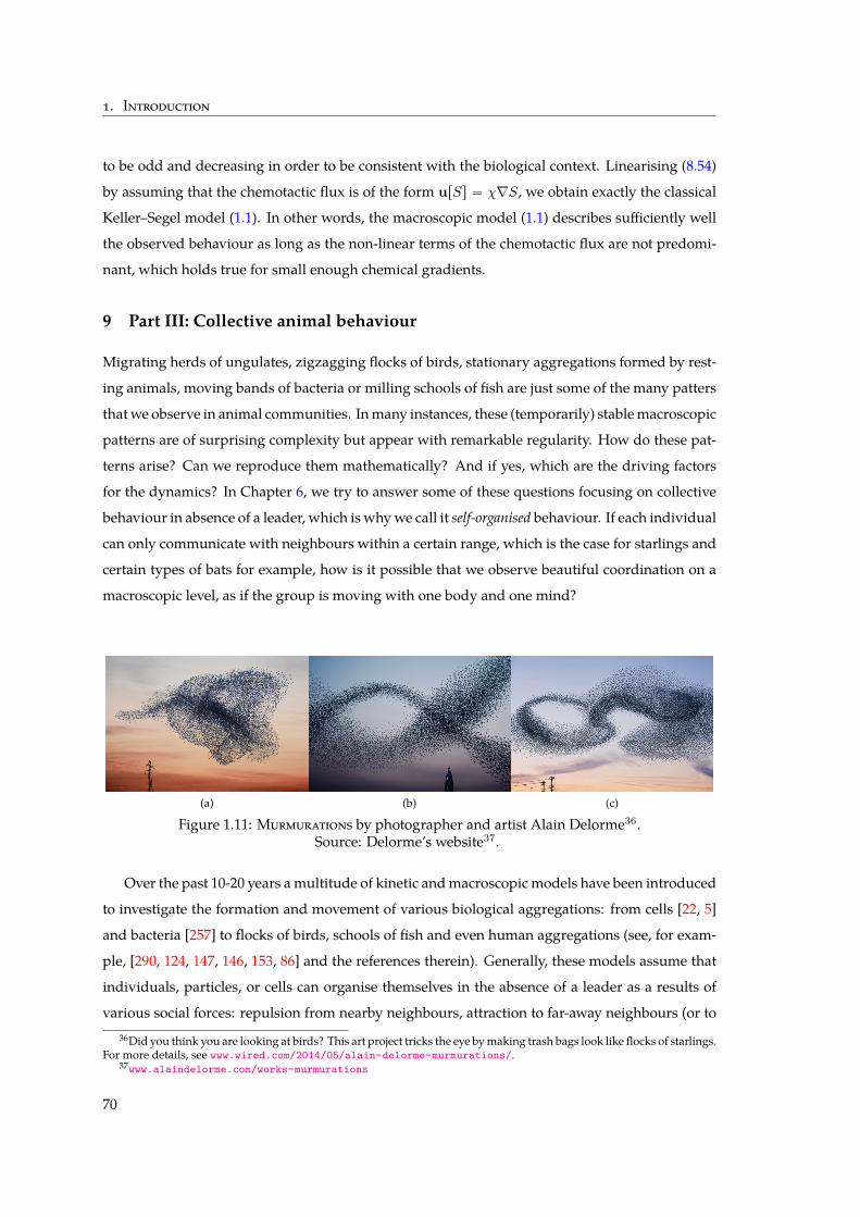
1. Introduction
to be odd and decreasing in order to be consistent with the biological context. Linearising (8.54)
by assuming that the chemotactic flux is of the form urSs “ χ∇S, we obtain exactly the classical
Keller–Segel model (1.1). In other words, the macroscopic model (1.1) describes sufficiently well
the observed behaviour as long as the non-linear terms of the chemotactic flux are not predomi-
nant, which holds true for small enough chemical gradients.
9 Part III: Collective animal behaviour
Migrating herds of ungulates, zigzagging flocks of birds, stationary aggregations formed by rest-
ing animals, moving bands of bacteria or milling schools of fish are just some of the many patters
thatwe observe in animal communities. Inmany instances, these (temporarily) stablemacroscopic
patterns are of surprising complexity but appear with remarkable regularity. How do these pat-
terns arise? Can we reproduce them mathematically? And if yes, which are the driving factors
for the dynamics? In Chapter 6, we try to answer some of these questions focusing on collective
behaviour in absence of a leader, which is whywe call it self-organised behaviour. If each individual
can only communicate with neighbours within a certain range, which is the case for starlings and
certain types of bats for example, how is it possible that we observe beautiful coordination on a
macroscopic level, as if the group is moving with one body and one mind?
(a) (b) (c)
Figure 1.11: Murmurations by photographer and artist Alain Delorme36.Source: Delorme’s website37.
Over the past 10-20 years amultitude of kinetic andmacroscopic models have been introduced
to investigate the formation and movement of various biological aggregations: from cells [22, 5]
and bacteria [257] to flocks of birds, schools of fish and even human aggregations (see, for exam-
ple, [290, 124, 147, 146, 153, 86] and the references therein). Generally, these models assume that
individuals, particles, or cells can organise themselves in the absence of a leader as a results of
various social forces: repulsion from nearby neighbours, attraction to far-away neighbours (or to36Did you think you are looking at birds? This art project tricks the eye bymaking trash bags look like flocks of starlings.
For more details, see www.wired.com/2014/05/alain-delorme-murmurations/.37www.alaindelorme.com/works-murmurations
70
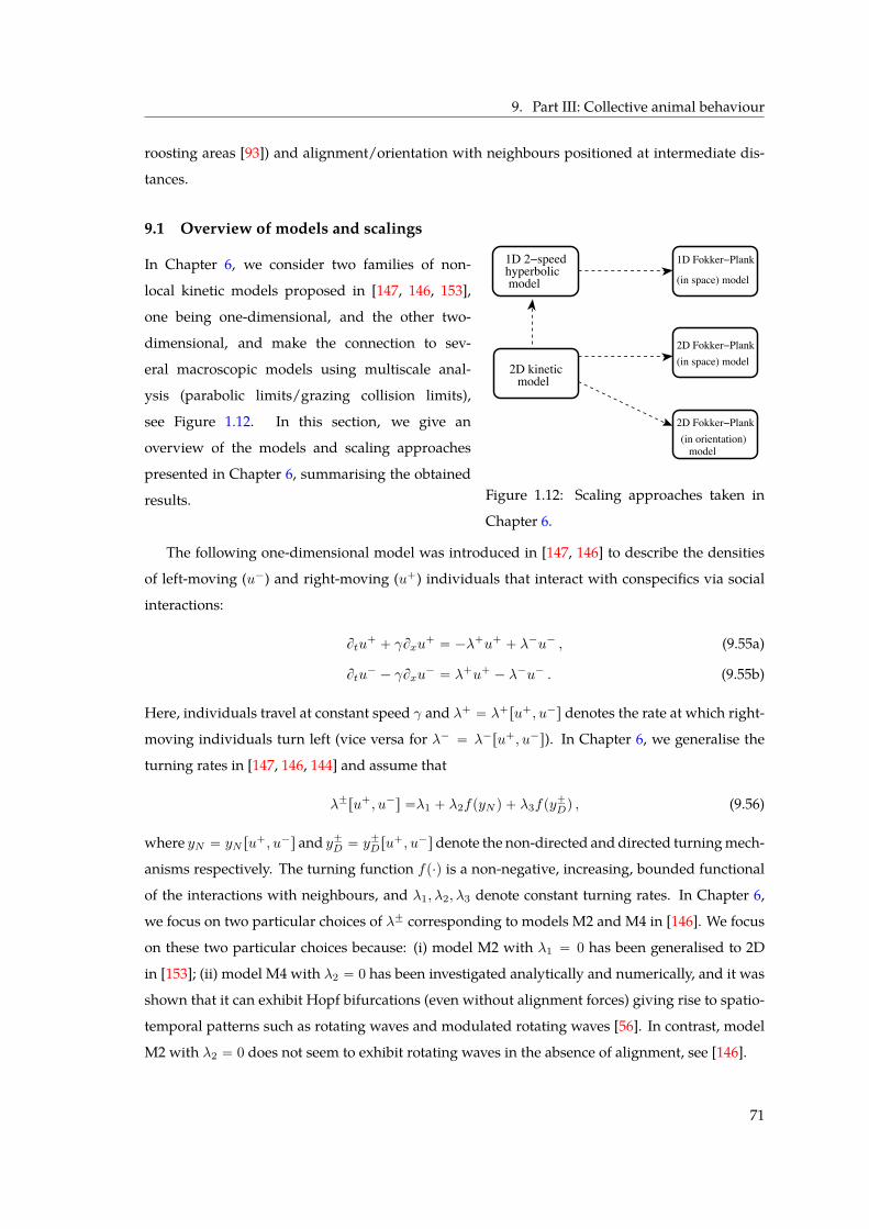
9. Part III: Collective animal behaviour
roosting areas [93]) and alignment/orientation with neighbours positioned at intermediate dis-
tances.
9.1 Overview of models and scalings
(in space) model
1D FokkerïPlank
(in space) model
2D FokkerïPlank(in orientation)
model
2D FokkerïPlank<+ /q=
f(y)=y
model2D kinetic
1D 2ïspeed
modelhyperbolic
Figure 1.12: Scaling approaches taken in
Chapter 6.
In Chapter 6, we consider two families of non-
local kinetic models proposed in [147, 146, 153],
one being one-dimensional, and the other two-
dimensional, and make the connection to sev-
eral macroscopic models using multiscale anal-
ysis (parabolic limits/grazing collision limits),
see Figure 1.12. In this section, we give an
overview of the models and scaling approaches
presented in Chapter 6, summarising the obtained
results.
The following one-dimensional model was introduced in [147, 146] to describe the densities
of left-moving (u´) and right-moving (u`) individuals that interact with conspecifics via social
interactions:
Btu` ` γBxu
` “ ´λ`u` ` λ´u´ , (9.55a)
Btu´ ´ γBxu
´ “ λ`u` ´ λ´u´ . (9.55b)
Here, individuals travel at constant speed γ and λ` “ λ`ru`, u´s denotes the rate at which right-
moving individuals turn left (vice versa for λ´ “ λ´ru`, u´s). In Chapter 6, we generalise the
turning rates in [147, 146, 144] and assume that
λ˘ru`, u´s “λ1 ` λ2fpyN q ` λ3fpy˘Dq , (9.56)
where yN “ yN ru`, u´s and y˘D “ y˘Dru
`, u´s denote the non-directed and directed turningmech-
anisms respectively. The turning function fp¨q is a non-negative, increasing, bounded functional
of the interactions with neighbours, and λ1, λ2, λ3 denote constant turning rates. In Chapter 6,
we focus on two particular choices of λ˘ corresponding to models M2 and M4 in [146]. We focus
on these two particular choices because: (i) model M2 with λ1 “ 0 has been generalised to 2D
in [153]; (ii) model M4 with λ2 “ 0 has been investigated analytically and numerically, and it was
shown that it can exhibit Hopf bifurcations (even without alignment forces) giving rise to spatio-
temporal patterns such as rotating waves and modulated rotating waves [56]. In contrast, model
M2 with λ2 “ 0 does not seem to exhibit rotating waves in the absence of alignment, see [146].
71
1. Introduction
We perform a parabolic scaling of the kinetic model (9.55) via pt, xq ÞÑ ptε2, xεq, using two
different scaling assumptions. Firstly, let us assume that individuals have a reduced perception of
their surroundings for small values of ε [143], that is, in rescaled variables
fε
´
y˘Dru, vs¯
“ εf´
y˘D“
u,
ż
xε
εBtu‰
¯
, fε
´
yN rus¯
“ εf´
yN rus¯
,
where u :“ u` ` u´ and v :“ γpu` ´ v´q. We obtain formally in the limit εÑ 0,
Btu “ D0Bxxu´ Bx
´
S0 uV puq¯
,
with diffusion rate D0 “ γ2p2λ1q and drift rate S0 “ λ3γp2λ1q explicitly given in terms of the
microscopic parameters. The expression for the velocity V puq differs for M2 or M4.
Secondly, if instead we assume f to be a linear function with a very weak directed turning be-
haviour, we can write
λ˘ “ λ1 ` λ2KN ˚ u` ε λ3y
˘Drus (9.57)
with yN rus “ KN ˚u for a social interaction kernelKN given in terms of attraction, repulsion and
alignment terms. By taking the limit ε Ñ 0 in (9.55) with scaling assumption (9.57), we obtain in
Chapter 6 a parabolic equation with density-dependent coefficients,
Btu “ Bx pDrusBxuq ´ Bx
´
Srusu`
y´Drus ´ y`Drus
˘
¯
, (9.58a)
Drus “γ2
2pλ1 ` λ2KN ˚ uqand Srus “
λ3γ
2pλ1 ` λ2KN ˚ uq. (9.58b)
A specific case of the 1D kinetic model (9.55) has been generalised to a 2D kinetic Boltzmann-
type equation in [153]:
Btu` γeφ ¨∇xu “
ż π
´π
T px, φ1, φqupx, φ1, tqdφ1 ´ λpx, φqupx, φ, tq . (9.59)
Here, upx, φ, tq is the total population density of individuals located at x “ px, yq P R2, moving at
a constant speed γ ą 0 in direction φ P r0, 2πq. The term eφ “ pcosφ, sinφq gives the movement
direction of individuals. The re-orientation terms, λpx, φq and T px, φ1, φq depend on the non-local
interactions with neighbours, which can be positioned in the repulsive, attractive, and alignment
ranges depicted in Fig. 1.13. Thus, these terms have three components each, corresponding to
the three social interactions, T px, φ1, φq “ Talpx, φ1, φq ` Tapx, φ1, φq ` Trpx, φ1, φq, and we define
λ “ř
j λj with
λjpx, φ1q “ż π
´π
Tjpx, φ1, φqdφ, j “ r, a, al .
For a detailed description of the turning mechanism, see Chapter 6 Section 3. In Chapter 6, we
generalise the turning mechanisms Tj , j “ tal, a, ru, from [153] by adding a constant turning rate,
72
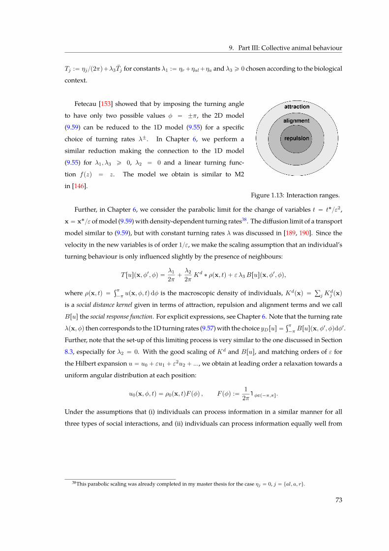
9. Part III: Collective animal behaviour
Tj :“ ηjp2πq`λ3Tj for constants λ1 :“ ηr`ηal`ηa and λ3 ě 0 chosen according to the biological
context.
Figure 1.13: Interaction ranges.
Fetecau [153] showed that by imposing the turning angle
to have only two possible values φ “ ˘π, the 2D model
(9.59) can be reduced to the 1D model (9.55) for a specific
choice of turning rates λ˘. In Chapter 6, we perform a
similar reduction making the connection to the 1D model
(9.55) for λ1, λ3 ě 0, λ2 “ 0 and a linear turning func-
tion fpzq “ z. The model we obtain is similar to M2
in [146].
Further, in Chapter 6, we consider the parabolic limit for the change of variables t “ t˚ε2,
x “ x˚ε ofmodel (9.59)with density-dependent turning rates38. The diffusion limit of a transport
model similar to (9.59), but with constant turning rates λ was discussed in [189, 190]. Since the
velocity in the new variables is of order 1ε, we make the scaling assumption that an individual’s
turning behaviour is only influenced slightly by the presence of neighbours:
T ruspx, φ1, φq “ λ1
2π `λ2
2π Kd ˚ ρpx, tq ` ε λ3Bruspx, φ1, φq,
where ρpx, tq “şπ
´πupx, φ, tqdφ is the macroscopic density of individuals, Kdpxq “
ř
j Kdj pxq
is a social distance kernel given in terms of attraction, repulsion and alignment terms and we call
Brus the social response function. For explicit expressions, see Chapter 6. Note that the turning rate
λpx, φq then corresponds to the 1D turning rates (9.57)with the choice yDrus “şπ
´πBruspx, φ1, φqdφ1.
Further, note that the set-up of this limiting process is very similar to the one discussed in Section
8.3, especially for λ2 “ 0. With the good scaling of Kd and Brus, and matching orders of ε for
the Hilbert expansion u “ u0 ` εu1 ` ε2u2 ` ..., we obtain at leading order a relaxation towards a
uniform angular distribution at each position:
u0px, φ, tq “ ρ0px, tqF pφq , F pφq :“ 12π1φPp´π,πs.
Under the assumptions that (i) individuals can process information in a similar manner for all
three types of social interactions, and (ii) individuals can process information equally well from
38This parabolic scaling was already completed in my master thesis for the case ηj “ 0, j “ tal, a, ru.
73
1. Introduction
left and right (symmetric perception), we obtain formally in the limit εÑ 0
Btρ “ ∇x . pD0rρs∇xρq ´∇x . pρkrρsq , (9.60a)
D0rρs “γ2
2pλ1 ` λ2Kd ˚ ρq, (9.60b)
krρspx, tq “ λ2πγ
λ1 ` λ2Kd ˚ ρ
ˆ
qrKdr pxq
x|x| ´ qaK
dapxq
x|x|
˙
˚ ρ , (9.60c)
where qr and qa denote the strength of repulsive and attractive forces respectively. For notational
convenience, we dropped the zero in ρ0. Note that this equation is similar to the 1D drift-diffusion
equation (9.58) obtained via the parabolic limit for linear social interactions. Indeed, the above
diffusive limit of the 2D model (9.59) reduces to a special case of the parabolic scaling of the 1D
model, which includes a λ2 term for non-directed turning.
Remark 9.1. For some particular choices of distance kernels Kd, the limiting parabolic model (9.60) can
be reduced to a particular case of the Keller–Segel type model (2.3) discussed in part I of this thesis. Let us
assume, for example, that the distance kernels are constant on the whole domain,
Kdj pxq “ 1, j “ al, a, r. (9.61)
This assumption corresponds to a setting in which individuals interact equally well with all other individuals
present in the entire domain. This is true locally for example if many individuals are packed in little space.
Under assumption (9.61) together with λ1 “ 0 and in the case when attractive and repulsive interactions
are not exactly equally strong qr ‰ qa (as they would cancel out otherwise), model (9.60) simplifies to the
aggregation-diffusion equation
Btρ “ D∆ρ` χ∇ . pρ p∇W ˚ ρqq , (9.62)
with W pxq “ |x| and D ą 0, χ ą 0 only depending on the parameters of the model and the total massş
ρ dx. Even for more general distance kernelsKdj , the social flux can be written in the form krρs “ ∇W ˚ρ
with the interaction potentialW behaving like |x| close to zero and decaying exponentially fast as |x| ÝÑ 8
(e.g. Morse potentials). Equation (9.62) models the behaviour of particles interacting through a pairwise
potential while diffusing with Brownian motion and is part of the family of aggregation-diffusion equations
analysed in Part I with linear diffusion (m “ 1) and a non-singular interaction kernel (k “ 1).
Finally, we consider the case where individuals turn only a small angle upon interactions with
neighbours, quantified by the parameter ε ! 1. This is biologically realistic as, for example,
many migratory birds follow favourable winds or magnetic fields [244] and social interactions
with neighbours might not have a considerable impact on directional changes of individuals. Fol-
lowing the discussion in Section 8.1, a grazing collision limit is well adapted when collisions with
74

9. Part III: Collective animal behaviour
small deviation dominate. In Chapter 6, we show that the Boltzmann-type equation (9.59) can
be reduced via a grazing collision limit to the following Fokker-Planck equation with non-local
advective and diffusive terms in the orientation space.
Btu` γeφ ¨∇xu “λ1
ˆ
12πρpx, tq ´ upx, φ, tq
˙
(9.63)
` Bφ
”
´ uCεru,x, φs ` BφpuDεru,x, φsqı
,
We omit here the details of Cεru,x, φs and Dεru,x, φs for brevity. While non-local 2D Fokker-
Planck models have been introduced in the past years in connection with self-organised aggrega-
tions, the majority of these models consider local diffusion [123, 12]. If we neglect second order
terms in ε (i.e. Dε « 0) and assume λ1 “ 0, equation (9.63) reduces to a Vlasov-type flocking
equation:
Btu` γeφ ¨∇xu` Bφ
”
uCεru, x, φsı
“ 0.
These type of models have been previously derived from individual-based models (Vicsek or
Cucker-Smale models) with or without noise [123, 179, 87].
9.2 Asymptotic preserving numerical methods
Finally, we investigate how two types of patterns (travelling and stationary aggregations) dis-
played by the 1D kinetic models, are preserved in the limit to macroscopic parabolic models. To
this end, we first analyse the local stability of spatially homogeneous patterns characterised by
individuals spread evenly over the domain, and show that local Hopf bifurcations are lost in the
parabolic limit. These Hopf bifurcations give rise to travelling aggregations (i.e. rotating waves).
We then test this observation numerically with the help of asymptotic preserving (AP) methods,
analysing changes in the patterns as the scaling coefficient ε is varied from ε “ 1 (for kinetic mod-
els) to ε “ 0 (for the limiting parabolic models). Understanding these transitions is important
when investigating biological phenomena that occur on multiple scales, since it allows to make
decisions regarding themodels that are most suitable to reproduce the observed dynamics. While
AP schemes have been derived since the late 1990’s to investigate the asymptotic dynamics of var-
ious transport models [201, 202, 88], they have only recently been applied to investigate multiscale
aspects of biological aggregations [102]. In Chapter 6, we show that some patterns (describing
stationary aggregations) are preserved in the limit ε Ñ 0, while others (describing moving ag-
gregations) are lost. To understand the loss of these patterns, we construct bifurcation diagrams.
Numerical and analytical investigation is still difficult for 2D non-local models, see [153].
75
1. Introduction
9.3 Conclusions and perspectives
The scaling approaches taken in Chapter 6 allow to simplify the kinetic models that incorporate
microscopic-level interactions (such as individuals’ speed and turning rates) to obtain parabolic
models described in terms of average speed and average turning behaviour. While for the kinetic
models the non-local interactions influence the turning rates, for the limit parabolic models the
non-local interactions influence the dispersion and the drift of the aggregations. In particular, the
assumption that individuals can turn randomly following the non-directional perception of neigh-
bours around them leads, in the macroscopic scaling, to density-dependent diffusion. Moreover,
this diffusion decreases with increasing population density. Biologically, this means that larger
animal groups are less likely to spread out. This phenomenon has been observed for various
species. For example, studies have shown that aggregations of locusts [55] or ants [21] can persist
only if the number of individuals is above a certain threshold.
The introduction in (9.56) of the term yN describing random non-directional turning (which
generalises the turning rates in [147]) is required in order to compare the parabolic limit models
in 1D and 2D. This suggests that even if the 2Dmodel (9.59) can be reduced to a special case of the
1D model (9.55) (as shown in [153]) there are more subtle differences between these non-local 1D
and 2D models. These differences can impact the types of patterns displayed by the 2D models –
an aspect that would be interesting to study in the future.
In Chapter 6, we use asymptotic preserving numerical methods to investigate the preservation
of patterns via the 1Dparabolic limit, but similar investigations could be performed for the grazing
collision limit. Moreover, as shown previously [146], model (9.55) can display manymore types of
complex spatio-temporal patterns than the two types of patterns investigated here. We choose to
focus on travelling and stationary aggregations since our aim is not to investigate how all possible
patterns are preserved by all these different scaling approaches. Rather, we want to show that by
taking these asymptotic limits, some patterns could be lost. Therefore, even if the macroscopic
models are simpler to investigate, they might not exhibit the same patterns as the kinetic models.
Our analysis aims at highlighting the usefulness of AP schemes to understand the bifurcation of
the solutions as one investigates the transition frommicroscopic-level to macroscopic-level aggre-
gation dynamics.
76
Part I
Keller-Segel-Type Aggregation-Diffusion
Equations
77
ἀνδρῶν γὰρ ἐπιφανῶν πᾶσα γῆ τάφος,
καὶ οὐ στηλῶν μόνον ἐν τῇ οἰκείᾳ σημαίνει ἐπιγραφή,
ἀλλὰ καὶ ἐν τῇ μὴ προσηκούσῃ ἄγραφος μνήμη παρ᾿ ἑκάστῳ
τῆς γνώμης μᾶλλον ἢ τοῦ ἔργου ἐνδιαιτᾶται.39
What you leave behind
is not what is engraved
in stone monuments,
but what is woven
into the lives of others40.
Pericles
39as quoted in Thucydides’History of the PeloponnesianWar, II.43.3 (5th century BC) fromPericles’ funeral oration. Literaltranslation by Steven Lattimore: "The whole earth is the tomb of famousmen, and not only inscriptions set up in their owncountry mark it but even in foreign lands an unwritten memorial, present not in monument but in mind, abides withineach man." [212, page 98]
40modern paraphrasing of the above as quoted in [249, page 118].
Chapter2
Ground States in the
Fair-Competition Regime
This chapter follows in most parts the article “Equilibria of homogeneous functionals in the fair-
competition regime”written in collaboration with Vincent Calvez1 and José A. Carrillo2, and pub-
lished in the special issue "Advances in Reaction-Cross-Diffusion Systems" of Nonlinear Analysis
TMA.
Chapter Summary
We consider macroscopic descriptions of particles where repulsion is modelled by non-
linear power-law diffusion and attraction by a homogeneous singular/non-singular kernel lead-
ing to variants of the Keller–Segel model of chemotaxis. We analyse the regime in which both
homogeneities scale the same with respect to dilations, that we coin as fair-competition. In the
singular kernel case, we show that existence of global equilibria can only happen at a certain
critical value and they are characterised as optimisers of a variant of HLS inequalities. We also
study the existence of self-similar solutions for the sub-critical case, or equivalently of optimisers
of rescaled free energies. These optimisers are shown to be compactly supported radially sym-
metric and non-increasing stationary solutions of the non-linear Keller–Segel equation. On the
other hand, we show that no radially symmetric non-increasing stationary solutions exist in the
non-singular kernel case, implying that there is no criticality. However, we show the existence of
positive self-similar solutions for all values of the parameter under the condition that diffusion
is not too fast. We finally illustrate some of the open problems in the non-singular kernel case
by numerical experiments.
1Unité de Mathématiques Pures et Appliquées, CNRS UMR 5669 and équipe-projet INRIA NUMED, École NormaleSupérieure de Lyon, Lyon, France.
2Department of Mathematics, Imperial College London, South Kensington Campus, London SW7 2AZ, UK.
79
2. Fair-Competition Regime
Chapter Content
1 Introduction . . . . . . . . . . . . . . . . . . . . . . . . . . . . . . . . . . . . . . . 81
2 Stationary states & main results . . . . . . . . . . . . . . . . . . . . . . . . . . . . 84
2.1 Stationary states: definition & basic properties . . . . . . . . . . . . . . . 84
2.2 Fair-competition regime: main results . . . . . . . . . . . . . . . . . . . . 88
3 Porous medium case k ă 0 . . . . . . . . . . . . . . . . . . . . . . . . . . . . . . 90
3.1 Global minimisers . . . . . . . . . . . . . . . . . . . . . . . . . . . . . . . 90
3.2 Regularity properties of global minimisers . . . . . . . . . . . . . . . . . 98
4 Fast diffusion case k ą 0 . . . . . . . . . . . . . . . . . . . . . . . . . . . . . . . . 110
4.1 Results in original variables . . . . . . . . . . . . . . . . . . . . . . . . . 111
4.2 Results in rescaled variables . . . . . . . . . . . . . . . . . . . . . . . . . 112
4.3 Numerical simulations in one dimension . . . . . . . . . . . . . . . . . . 118
A Appendix: Properties of ψk . . . . . . . . . . . . . . . . . . . . . . . . . . . . . . 120
Haba na haba hujaza kibaba.
Little by little fills up the measure.
Kiswahili proverb
80
1. Introduction
1 Introduction
The goal of this chapter is to investigate properties of the following class of homogeneous func-
tionals, defined for centred probability densities ρpxq, belonging to suitable Lp-spaces, and some
interaction strength coefficient χ ą 0 and diffusion powerm ą 0:
Fm,krρs “ż
RNUm pρpxqq dx` χ
ij
RNˆRN
ρpxqWkpx´ yqρpyq dxdy
:“ Umrρs ` χWkrρs , (1.1)
ρpxq ě 0 ,ż
RNρpxq dx “ 1 ,
ż
RNxρpxq dx “ 0 ,
with
Umpρq “
$
’
’
&
’
’
%
1Npm´ 1qρ
m , if m ‰ 1
1Nρ log ρ , if m “ 1
,
and
Wkpxq “
$
’
&
’
%
|x|k
k, if k P p´N,Nqzt0u
log |x| , if k “ 0.
The conditions on k imply that the kernelWkpxq is locally integrable in RN . The centre of mass is
assumed to be zero since the free energy functional is invariant by translation.
There exists a strong link between the aforementioned functional (1.1) and the following family
of partial differential equations modelling self-attracting diffusive particles at the macroscopic
scale,$
’
&
’
%
Btρ “1N
∆ρm ` 2χ∇ ¨ pρ∇Skq , t ą 0 , x P RN ,
ρpt “ 0, xq “ ρ0pxq ě 0 ,ż
RNρ0pxq dx “ 1 ,
ż
RNxρ0pxq dx “ 0 ,
(1.2)
where we define the mean-field potential Skpxq :“ Wkpxq ˚ ρpxq. For k ą 1 ´ N , the gradient
∇Sk :“ ∇ pWk ˚ ρq is well defined. For ´N ă k ď 1´N however, it becomes a singular integral,
and we thus define it via a Cauchy principal value. Hence, the mean-field potential gradient in
equation (1.2) is given by
∇Skpxq :“
$
’
’
&
’
’
%
∇Wk ˚ ρ , if k ą 1´N ,
ż
RN∇Wkpx´ yq pρpyq ´ ρpxqq dy , if ´N ă k ď 1´N .
(1.3)
The noticeable characteristic of the class of PDEs (1.2) and the functional Fm,k consists in the com-
petition between the diffusion (possibly non-linear), and the non-local, quadratic non-linearity
which is due to the self-attraction of the particles through themean-field potential Sk. The param-
eter χ ą 0 measures the strength of the interaction and scales with the mass of solution densities.
81
2. Fair-Competition Regime
The strong connection between the functional Fm,k and the PDE (1.2) is due to the fact that
the functional Fm,k is non-increasing along the trajectories of the system. Namely Fm,k is the free
energy of the system and it satisfies at least formally
d
dtFm,krρptqs “ ´
ż
RNρpt, xq
ˇ
ˇ
ˇ
ˇ
∇ˆ
m
Npm´ 1qρpt, xqm´1 ` 2χWkpxq ˚ ρpt, xq
˙ˇ
ˇ
ˇ
ˇ
2dx .
Furthermore, the system (1.2) is the formal gradient flow of the free energy functional (1.1) when
the space of probability measures is endowed with the Euclidean Wasserstein metric W. This
means that the family of PDEs (1.2) can be written as
Btρptq “ ∇ ¨ pρptq∇Tm,krρptqsq “ ´∇WFm,krρptqs ,
where Tm,krρs denotes the first variation of the energy functional in the set of probability densities:
Tm,krρspxq :“ δFm,kδρ
rρspxq “m
Npm´ 1qρm´1pxq ` 2χWkpxq ˚ ρpxq . (1.4)
This illuminating statement has been clarified in the seminal paper by Otto [248] for the porous
medium equation, and generalised to a large family of equations subsequently in [96, 3, 97], we
refer to [295, 3] for a comprehensive presentation of this theory of gradient flows in Wasserstein
metric spaces, particularly in the convex case. Let us mention that such a gradient flow can be
constructed as the limit of discrete in time steepest descent schemes. Performing gradient flows
of a convex functional is a natural task, and suitable estimates from below on the right notion of
Hessian of Fm,k translate into a rate of convergence towards equilibrium for the PDE [295, 96, 3].
However, performing gradient flows of non-convex functionals is much more delicate, and one
has to seek compensations. Such compensations do exist in our case, and we will observe them
at the level of existence of minimisers for the free energy functional Fm,k and stationary states of
the family of PDEs (1.2) in particular regimes.
The family of non-local problems (1.2) has been intensively studied in various contexts arising
in physics and biology. The two-dimensional logarithmic case pm “ 1, k “ 0q is the so-called
Keller–Segel system in its simplest formulation [196, 197, 243, 194, 136, 41, 256]. It has been pro-
posed as a model for chemotaxis in cell populations. Cells may interact with each other by secret-
ing a chemical substance to attract cells around them. This occurs for instance during the star-
vation stage of the slime mould Dictyostelium discoideum. More generally, chemotaxis is widely
observed in various biological fields (morphogenesis, bacterial self-organisation, inflammatory
processes among others). The two- and three-dimensional configurations with Newtonian inter-
action pm “ 1, k “ 2´Nq are the so-called Smoluchowski-Poisson system arising in gravitational
physics. It describes macroscopically a density of particles subject to a self-sustained gravitational
field [106, 107].
82
1. Introduction
Let us describe in more detail the two-dimensional Keller–Segel system as the analysis of its
peculiar structure will serve as a guideline to understand the other cases. In fact, the functional
(1.1) pm “ 1, k “ 0q is bounded from below if and only if χ “ 1. The gradient flow is also
subject to a remarkable dichotomy, well described mathematically. The density exists globally in
time if χ ă 1 (diffusion overcomes self-attraction), whereas blow-up occurs in finite time when
χ ą 1 (self-attraction overwhelms diffusion). This transition has been first formulated in [113].
Mathematical contributions are [194] for the existence part, [242] for the radial case, and [136, 41]
in the full space. The critical case χ “ 1 was analysed further in [40, 37, 75] in terms of stability of
stationary states.
The effect of substituting linear diffusion by non-linear diffusionwithm ą 1 in two dimensions
and higher was described in [61, 277] where it is shown that solutions exist globally in time for all
values of the parameter χ ą 0. The role of both non-linear diffusion and non-local aggregation
termswas clarified in [39], see also [276], where the authors find that there is a similar dichotomy to
the two-dimensional classical Keller–Segel case pN “ 2,m “ 1, k “ 0q, for awhole range of param-
eters, choosing the non-local term as the Newtonian potential, pN ě 3,m “ 2´ 2N, k “ 2´Nq.
Themain difference is that the stationary states found for the critical case are compactly supported.
Choosing the non-local term as the Newtonian potential, this range of parameters can be under-
stood as fixing the non-linear diffusion such that both terms in the functional Fm,k scale equally
for mass-preserving dilations. This mass-preserving dilation homogeneity of the functional Fm,kis shared by the range of parameters pm, kqwith Npm´ 1q ` k “ 0 for all dimensions,m ą 0 and
k P p´N,Nq. We call this range of parameters the fair-competition regime, since both terms are
competing each other at equal foot.
In this chapter, we will analyse the properties of the functional Fm.k in relation to global min-
imisers and its relation to stationary states of (1.2). We will first define properly the notion of sta-
tionary states to (1.2) and analyse their basic properties in Section 2. Wewill also state and explain
themain results of this chapter once the different regimes have been introduced. We postpone fur-
ther discussion of the related literature to Section 2. Section 3 is devoted to the fair-competition
regime with k ă 0 for which we show a similar dichotomy to [39] in the whole range k P p´N, 0q
including themost singular cases. We show that stationary states exist only for a critical value of χ
and that they are compactly supported, bounded, radially symmetric decreasing and continuous
functions. Moreover, we show that they are global minimisers of Fm.k. The sub-critical case is also
analysed in scaled variables and we show the existence of global minimisers with the properties
above leading to the existence of self-similar solutions in original variables. The critical parameter
is characterised by a variant of HLS inequalities as in [39]. Let us mention that the regularity re-
sults need a careful treatment of the problem in radial coordinates involving non-trivial properties
83
2. Fair-Competition Regime
of hypergeometric functions. The properties of the kernel in radial coordinates are postponed to
the Appendix A.
In Section 4, we analyse the case k ą 0. Let us mention that there are no results in the literature
to our knowledge concerning the case k P p0, Nq in which 0 ă m “ 1 ´ kN ă 1. There is
one related result in [116] for the limiting case in one dimension taking m “ 0, corresponding to
logarithmic diffusion, and k “ 1. They showed that no criticality is present in that case as solutions
to (1.2) with pm “ 0, k “ 1q are globally defined in time for all values of the parameter χ ą 0. We
show that no radially symmetric non-increasing stationary states and no radially symmetric non-
increasing global minimisers exist in original variables for all values of the critical parameter χ
and for k P p0, Nq while we show the existence of stationary states for all values of the critical
parameter χ in scaled variables for k P p0, 1s. In this sense, we show that there is no criticality
for k ą 0. A full proof of non-criticality involves the analysis of the minimisation problem in
scaled variables as for k ă 0 showing that global minimisers exist in the right functional spaces
for all values of the critical parameter and that they are indeed stationary states. This is proven
in one dimension in Chapter 3 by optimal transport techniques and postponed for further future
investigations in general dimension. We finally illustrate these results by numerical experiments
in one dimension corroborating the absence of critical behaviour for k ą 0.
2 Stationary states & main results
2.1 Stationary states: definition & basic properties
Let us define precisely the notion of stationary states to the aggregation equation (1.2).
Definition 2.1. Given ρ P L1`
`
RN˘
XL8`
RN˘
with ||ρ||1 “ 1, it is a stationary state for the evolution
equation (1.2) if ρm P W1,2loc
`
RN˘
, ∇Sk P L1loc
`
RN˘
, and it satisfies
1N
∇ρm “ ´2χ ρ∇Sk (2.5)
in the sense of distributions in RN . If ´N ă k ď 1 ´ N , we further require ρ P C0,α `RN˘
with
α P p1´ k ´N, 1q.
We start by showing that the function Sk and its gradient defined in (1.3) satisfy even more
than the regularity ∇Sk P L1loc
`
RN˘
required in Definition 2.1.
Lemma 2.2. Let ρ P L1`
`
RN˘
X L8`
RN˘
with ||ρ||1 “ 1. If 0 ă k ă N , we additionally assume
|x|kρ P L1 `RN˘
. Then the following regularity properties hold:
i) Sk P L8loc`
RN˘
for 0 ă k ă N and Sk P L8`
RN˘
for ´N ă k ă 0.
84
2. Stationary states & main results
ii) ∇Sk P L8loc`
RN˘
for 1 ă k ă N and ∇Sk P L8`
RN˘
for ´N ă k ă 0 and 0 ă k ď 1, assuming
additionally ρ P C0,α `RN˘
with α P p1´ k ´N, 1q in the range ´N ă k ď 1´N .
Proof. A direct decomposition in near- and far-field sets A :“ ty : |x´ y| ď 1u and B :“ RN ´ A
yields for ´N ă k ă 0 and x P RN ,
|Skpxq| ď
ż
RN|Wkpx´ yq|ρpyq dy ď
1|k|
ż
A|x´ y|kρpyq dy `
1|k|
ż
Bρpyq dy
ď1|k|
ˆ
σNk `N
||ρ||8 ` 1˙
ă 8 ,
where σN “ 2πpN2qΓpN2q denotes the surface area of the N -dimensional unit ball. Locally,
boundedness extends to the fast diffusion regime 0 ă k ă N by using the inequality
|x´ y|k ď η`
|x|k ` |y|k˘
, η “ maxt1, 2k´1u . (2.6)
This inequality follows directly from splitting into cases k ă 1 and k ą 1. The inequality |x´y|k ď
|x|k ` |y|k is true for any k P p0, 1s with x, y P RN by direct inspection. For N ą 1 and k P p1, Nq,
we have by convexity |x´ y|k ď 2k´1 `|x|k ` |y|k˘
, for any x, y P RN , and so (2.6) holds true.
Similarly, in order to prove ii) for 1´N ă k ď 1 and x P RN , we estimate ∇Sk as
|∇Skpxq| ďż
RN|∇Wkpx´ yq|ρpyq dy ď
ż
A|x´ y|k´1ρpyq dy `
ż
Bρpyq dy
ď
ˆ
σNk `N ´ 1 ||ρ||8 ` 1
˙
ă 8 .
In the Cauchy integral range´N ă k ď 1´N , we additionally require a certain Hölder regularity,
yielding
|∇Skpxq| “ˇ
ˇ
ˇ
ˇ
ż
A∇Wkpx´ yq pρpyq ´ ρpxqq dy `
ż
B∇Wkpx´ yq pρpyq ´ ρpxqq dy
ˇ
ˇ
ˇ
ˇ
ď
ż
A|∇Wkpx´ yq| |ρpyq ´ ρpxq| dy `
ż
B|∇Wkpx´ yq|ρpyq dy
ď rρsC0,α
ż
A|x´ y|k´1|x´ y|α dy `
ż
Bρpyq dy ă 8 ,
where rρsC0,α denotes theα-Hölder semi-normof ρ, andwhere the termş
B ∇Wkpx´yq dy vanishes
by anti-symmetry. For 1 ă k ă N and x in some compact set, we have
|∇Skpxq| ďż
A|x´ y|k´1ρpyq dy `
ż
B|x´ y|k´1ρpyq dy
ďσN
k `N ´ 1 ||ρ||8 `ż
B|x´ y|kρpyq dy
which concludes∇Sk P L8loc`
RN˘
using (2.6) and the fact that the kthmoment of ρ is bounded.
We will prove that for certain cases there are no stationary states to (1.2) in the sense of Def-
inition 2.1, for instance for the sub-critical classical Keller–Segel model in two dimensions [41].
85
2. Fair-Competition Regime
However, the scale invariance of (1.2) motivates us to look for self-similar solutions instead. To
this end, we rescale equation (1.2) to a non-linear Fokker–Planck type equation as in [100]. Let us
define
upt, xq :“ αN ptqρ pβptq, αptqxq ,
where ρpt, xq solves (1.2) and the functions αptq, βptq are to be determined. If we assume up0, xq “
ρp0, xq, then upt, xq satisfies the rescaled drift-diffusion equation$
’
&
’
%
Btu “1N∆um ` 2χ∇ ¨ pu∇Skq `∇ ¨ pxuq , t ą 0 , x P RN ,
upt “ 0, xq “ ρ0pxq ě 0 ,ż 8
´8
ρ0pxq dx “ 1 ,ż 8
´8
xρ0pxq dx “ 0 ,(2.7)
for the choices
αptq “ et, βptq “
$
’
&
’
%
12´k
`
ep2´kqt ´ 1˘
, if k ‰ 2,
t, if k “ 2,
and with ∇Sk given by (1.3) with u instead of ρ. By differentiating the centre of mass of u, we see
easily thatż
RNxupt, xq dx “ e´t
ż
RNxρ0pxq dx “ 0 , @t ą 0 ,
and so the initial zero centre of mass is preserved for all times. Self-similar solutions to (1.2) now
correspond to stationary solutions of (2.7). Similar to Definition 2.1, we state what we exactly
mean by stationary states to the aggregation equation (2.7).
Definition 2.3. Given u P L1`
`
RN˘
XL8`
RN˘
with ||u||1 “ 1, it is a stationary state for the evolution
equation (2.7) if um P W1,2loc
`
RN˘
, ∇Sk P L1loc
`
RN˘
, and it satisfies
1N
∇um “ ´2χ u∇Sk ´ x u (2.8)
in the sense of distributions in RN . If ´N ă k ď 1 ´ N , we further require u P C0,α `RN˘
with
α P p1´ k ´N, 1q.
From now on, we switch notation from u to ρ for simplicity, it should be clear from the context
if we are in original or rescaled variables. In fact, stationary states as defined above have even
more regularity:
Lemma 2.4. Let k P p´N,Nqzt0u and χ ą 0.
(i) If ρ is a stationary state of equation (1.2) with |x|kρ P L1 `RN˘
in the case 0 ă k ă N , then ρ is
continuous on RN .
(ii) If ρresc is a stationary state of equation (2.7) with |x|kρresc P L1 `RN˘
in the case 0 ă k ă N , then
ρresc is continuous on RN .
86
2. Stationary states & main results
Proof. (i) First, note that ∇Sk P L8loc`
RN˘
by Lemma 2.2, and therefore, ρ∇Sk P L1loc
`
RN˘
X
L8loc`
RN˘
. Hence, we get by interpolation that ∇ ¨`
ρ∇Sk˘
P W´1,ploc
`
RN˘
for all 1 ă p ă 8.
Recall from Definition 2.1 that ρm is a weak W1,2loc
`
RN˘
solution of
1N
∆ρm “ ´2χ∇ ¨`
ρ∇Sk˘
in RN , and so ρm is in fact a weak solution in W1,ploc
`
RN˘
for all 1 ă p ă 8 by classic el-
liptic regularity. Using Morrey’s inequality, we deduce that ρm belongs to the Hölder space
C0,αloc
`
RN˘
with α “ pp ´ NqN for any N ă p ă 8, and thus ρm P C`
RN˘
. Hence, ρ itself
is continuous as claimed.
(ii) Sincexρresc P L1loc
`
RN˘
XL8loc`
RN˘
, we obtain again by interpolation∇¨pxρrescq P W´1,ploc
`
RN˘
for all 1 ă p ă 8. By Definition 2.3, ρmresc is a weak W1,2loc
`
RN˘
solution of
1N
∆ρmresc “ ´2χ∇ ¨`
ρresc∇Sk˘
´∇ ¨ pxρrescq
in RN , and so ρmresc is again a weak solution in W1,ploc
`
RN˘
for all 1 ă p ă 8 by classic elliptic
regularity. We conclude as in original variables.
In the case k ă 0, we furthermore have a non-linear algebraic equation for stationary states:
Corollary 2.5 (Necessary Condition for Stationary States). Let k P p´N, 0q and χ ą 0.
(i) If ρ is a stationary state of equation (1.2), then ρ P W1,8 `
RN˘
and it satisfies
ρpxqm´1 “Npm´ 1q
m
`
Ckrρspxq ´ 2χ Skpxq˘
`, @x P RN , (2.9)
where Ckrρspxq is constant on each connected component of supp pρq.
(ii) If ρresc is a stationary state of equation (2.7), then ρresc P W1,8loc
`
RN˘
and it satisfies
ρrescpxqm´1 “
Npm´ 1qm
ˆ
Ck,rescrρspxq ´ 2χ Skpxq ´|x|2
2
˙
`
, @x P RN , (2.10)
where Ck,rescrρspxq is constant on each connected component of supp pρrescq.
Proof. (i) For a stationary state ρ of equation (1.2), let us define the set
Ω “
x P RN : ρpxq ą 0(
.
Since ρ is continuous by Lemma 2.4, Ω is an open set with countably many open, possibly
unbounded connected components. Let us take any bounded smooth connected open subset
U such that U Ă Ω. By continuity, ρ is bounded away from zero in U , and thus ∇ρm´1 “
87
2. Fair-Competition Regime
m´1mρ ∇ρm holds in the distributional sense in U . From (2.5) in the definition of stationary
states, we conclude that
∇ˆ
m
Npm´ 1q ρm´1 ` 2χ Sk
˙
“ 0 , (2.11)
in the sense of distributions in Ω. Hence, the functionCkrρspxq :“ mNpm´1q ρ
m´1pxq`2χ Skpxq
is constant in each connected component of Ω, and so (2.9) follows. Additionally, it follows
from (2.11) that for any x P RN
ˇ
ˇ∇ρm´1pxqˇ
ˇ “2χNpm´ 1q
m
ˇ
ˇ∇Skpxqˇ
ˇ ď c
for some constant c ą 0 since Sk P W1,8 `
RN˘
by Lemma 2.2. Sincem P p1, 2q, we conclude
ρ P W1,8 `
RN˘
.
(ii) We follow the same argument for a stationary state ρresc of the rescaled equation (2.7) and
using (2.8) in Definition 2.3, we obtain
∇ˆ
m
Npm´ 1q ρm´1resc ` 2χ Sk `
|x|2
2
˙
“ 0 ,
in the sense of distributions in Ω. Here, the function Ck,rescrρrescspxq :“ mNpm´1q ρ
m´1resc pxq `
2χ Skpxq ` |x|2
2 is again constant in each connected component of supp pρrescq. Similarly, it
follows from Lemma 2.2 that for any ω ą 0 and x P Bp0, ωq,
ˇ
ˇ∇ρm´1resc pxq
ˇ
ˇ “Npm´ 1q
m
`
2χˇ
ˇ∇Skpxqˇ
ˇ` |x|˘
ď c
for some constant c ą 0, and so ρresc P W1,8loc
`
RN˘
.
2.2 Fair-competition regime: main results
It is worth noting that the functional Fm,krρs possesses remarkable homogeneity properties, see
Chapter 1 Section 3.1. Wewill here only concentrate on the fair-competition regimeNpm´1q`k “
0, and denote the corresponding energy functional by Fkrρs “ F1´kN,krρs. For a definition of
the different regimes and detailed explanations and references, see Chapter 1 Definition 3.1. An
overview of the parameter space pk,mq and the different regimes is given in Chapter 1 Figure 1.4.
Notice that the functional Fk is homogeneous in this regime, i.e.,
Fkrρλs “ λ´kFkrρs . (2.12)
The analysis in the fair-competition regime depends on the sign of k, see Chapter 1 Definition 3.7,
and we therefore split our investigations into the porous medium case (k ă 0), and the fast diffu-
sion case (k ą 0). More information on the logarithmic case (k “ 0) can be found in [62]. When
88
2. Stationary states & main results
dealing with the energy functional Fk, we work in the set of non-negative normalised densities,
Y :“"
ρ P L1`
`
RN˘
X Lm`
RN˘
: ||ρ||1 “ 1 ,ż
xρpxq dx “ 0*
.
In rescaled variables, equation (2.7) is the formal gradient flow of the rescaled free energy func-
tional Fk,resc, which is complemented with an additional quadratic confinement potential,
Fk,rescrρs “ Fkrρs `12Vrρs , Vrρs “
ż
RN|x|2ρpxq dx .
Defining the sets
Y2 :“ tρ P Y : Vrρs ă 8u , Yk :“"
ρ P Y :ż
RN|x|kρpxq dx ă 8
*
,
we see that Fk,resc is well-defined and finite on Y2 for k ă 0 and on Y2,k :“ Y2 X Yk for k ą 0.
Thanks to the formal gradient flow structure in the EuclideanWasserstein metricW, we can write
the rescaled equation (2.7) as
Btρ “ ∇ ¨ pρ∇Tk,rescrρsq “ ´∇WFk,rescrρs ,
where Tk,resc denotes the first variation of the rescaled energy functional,
Tk,rescrρspxq :“ Tkrρspxq `|x|2
2 (2.13)
with Tk as defined in (1.4). In this chapter, we prove the following results:
Theorem 2.6 (The Critical Porous Medium Regime). In the porous medium regime k P p´N, 0q and
for critical interaction strengths χ “ χc, there exist global minimisers of Fk and they are radially sym-
metric non-increasing, compactly supported and uniformly bounded. Furthermore, all stationary states
with bounded second moment are global minimisers of the energy functional Fk, and conversely, all global
minimisers of Fk are stationary states of (1.2).
Theorem 2.7 (The Sub-Critical Porous Medium Regime). In the porous medium regime k P p´N, 0q
and for sub-critical interaction strengths 0 ă χ ă χc, no stationary states exist for equation (1.2) and
no minimisers exist for Fk. In rescaled variables, all stationary states are continuous and compactly sup-
ported. There exist global minimisers of Fk,resc and they are radially symmetric non-increasing and uni-
formly bounded stationary states of equation (2.7).
Remark 2.8. Due to the homogeneity (2.12) of the functionalFk, each global minimiser gives rise to a family
of global minimisers for χ “ χc by dilation since they have zero energy, see (3.19). It is an open problem to
show that there is a unique global minimiser for χ “ χc modulo dilations. This uniqueness was proven in
the Newtonian case in [302], but is still an open problem in the general. Notice that from uniqueness one
obtains the full set of stationary states with bounded second moment for (1.2) as a by-product.
89
2. Fair-Competition Regime
In contrast, in rescaled variables, we do not know if stationary states with second moment bounded are
among global minimisers ofFk,resc for the sub-critical case 0 ă χ ă χc except in one dimension, see Chapter
3. It is also an open problem to show the uniqueness of radially symmetric stationary states of the rescaled
equation (2.7) for N ě 2.
Theorem 2.9 (The Fast Diffusion Regime). In the fast diffusion regime k P p0, Nq equation (1.2)
has no radially symmetric non-increasing stationary states with kth moment bounded, and there are no
radially symmetric non-increasing global minimisers for the energy functional Fk for any χ ą 0. In
rescaled variables, radially symmetric non-increasing stationary states can only exist if 0 ă k ă 2, that is
pN ´ 2qN ă m ă 1. Similarly, global minimisers with finite energy Fk,resc can only exist in the range
0 ă k ă 2Np2 ` Nq, that is Np2 ` Nq ă m ă 1. For k P p0, 1s, there exists a continuous radially
symmetric non-increasing stationary state of the rescaled equation (2.7).
3 Porous medium case k ă 0
In the porous medium case, we have ´N ă k ă 0 and hence 1 ă m ă 2. Our aim in this
section is to make a connection between global minimisers of the functionals Fk and Fk,resc and
stationary states of equations (1.2) and (2.7) respectively. We will show that in the critical case
χ “ χc, global minimisers and stationary states are equivalent for original variables. In the sub-
critical case 0 ă χ ă χc, all minimisers of Fk,resc will turn out to be stationary states of the rescaled
equation (2.7).
3.1 Global minimisers
A key ingredient for the analysis in the porous medium case are certain functional inequalities
which are variants of the Hardy-Littlewood-Sobolev (HLS) inequality, also known as the weak
Young’s inequality [218, Theorem 4.3]:ij
RNˆRN
fpxq|x´ y|kfpyq dxdy ď CHLSpp, q, kqfpfq , (3.14)
1p`
1q“ 2` k
N, p, q ą 1 , k P p´N, 0q .
Theorem 3.1 (Variation of HLS). Let k P p´N, 0q. For f P L1 `RN˘
X Lm`
RN˘
, we haveˇ
ˇ
ˇ
ˇ
ˇ
ˇ
ij
RNˆRN
fpxq|x´ y|kfpyqdxdy
ˇ
ˇ
ˇ
ˇ
ˇ
ˇ
ď C˚||f ||N`kN
1 ||f ||mm, (3.15)
where C˚pk,Nq is defined as the best constant.
Proof. The inequality is a direct consequence of the standard HLS inequality (3.14) by choosing
p “ q “ 2N2N`k , and of Hölder’s inequality. For k P p´N, 0q and for any f P L1 `RN
˘
X Lm`
RN˘
,
90
3. Porous medium case k ă 0
we haveˇ
ˇ
ˇ
ˇ
ˇ
ˇ
ij
RˆR
fpxq|x´ y|kfpyqdxdy
ˇ
ˇ
ˇ
ˇ
ˇ
ˇ
ď CHLS ||f ||2p ď CHLS ||f ||
N`kN
1 ||f ||mm.
Consequently, C˚ is finite and bounded from above by CHLS .
Now, let us compute explicitly the energy of stationary states:
Lemma 3.2. For any´N ă k ă 0 and χ ą 0, all stationary states ρ of (1.2)with |x|2ρ P L1 `RN˘
satisfy
Fk rρs “ 0.
Proof. Integrating (2.5) against x, we obtain for 1´N ă k ă 0:
1N
ż
RNx ¨∇ρm “ ´2χ
ij
RNˆRN
x ¨ px´ yq|x´ y|k´2ρpxqρpyq dxdy
´
ż
RNρm “ ´χ
ij
RNˆRN
px´ yq ¨ px´ yq|x´ y|k´2ρpxqρpyq dxdy
1Npm´ 1q
ż
RNρm “ ´χ
ij
RNˆRN
|x´ y|k
kρpxqρpyq dxdy , (3.16)
and the result immediately follows. For´N ă k ď 1´N , the term ∇Sk is a singular integral, and
thus writes
∇Skpxq “ limεÑ0
ż
Bcpx,εq
|x´ y|k´2px´ yqρkpyq dy
“
ż
R|x´ y|k´2px´ yq pρkpyq ´ ρkpxqq dy .
The singularity disappears when integrating against x,ż
RNx ¨∇Skpxqρkpxq dx “
12
ij
RNˆRN
|x´ y|kρkpxqρkpyq dxdy . (3.17)
In order to prove (3.17), let us define
fεpxq :“ż
Bcpx,εq
x ¨∇xWkpx´ yqρkpyq dy.
Then by definition of the Cauchy Principle Value, fεpxq Ñ x ¨∇Skpxq pointwise for almost every
x P RN as εÑ 0. Further, we have for 0 ă ε ă 1,
|fεpxq| ď |x|
ˇ
ˇ
ˇ
ˇ
ˇ
ż
Bcpx,εqXBpx,1q∇xWkpx´ yqρkpyq dy `
ż
Bcpx,εqXBcpx,1q∇xWkpx´ yqρkpyq dy
ˇ
ˇ
ˇ
ˇ
ˇ
ď |x|
˜ˇ
ˇ
ˇ
ˇ
ˇ
ż
Bcpx,εqXBpx,1q∇xWkpx´ yqρkpyq dy
ˇ
ˇ
ˇ
ˇ
ˇ
`
ż
|x´y|ě1|x´ y|k´1ρkpyq dy
¸
ď |x|
˜ˇ
ˇ
ˇ
ˇ
ˇ
ż
Bcpx,εqXBpx,1q∇xWkpx´ yqρkpyq dy
ˇ
ˇ
ˇ
ˇ
ˇ
` 1¸
91
2. Fair-Competition Regime
Since ∇Wk is anti-symmetric, the termş
Bcpx,εqXBpx,1q∇xWkpx ´ yq dy vanishes and we are thus
free to subtract it. Using the fact that ρk P C0,αpRN q for some α P p1´ k ´N, 1q, we haveˇ
ˇ
ˇ
ˇ
ˇ
ż
Bcpx,εqXBpx,1q∇xWkpx´ yqρkpyq dy
ˇ
ˇ
ˇ
ˇ
ˇ
“
ˇ
ˇ
ˇ
ˇ
ˇ
ż
Bcpx,εqXBpx,1q∇xWkpx´ yq rρkpyq ´ ρkpxqs dy
ˇ
ˇ
ˇ
ˇ
ˇ
ď
ż
Bcpx,εqXBpx,1q|x´ y|k´1 |ρkpyq ´ ρkpxq| dy
ď
ż
Bcpx,εqXBpx,1q|x´ y|k`α´1 dy
“σN
k `N ´ 1` α`
1´ εk`N´1`α˘
ďσN
k `N ´ 1` α .
We conclude that |fεpxq| ď´
σN`k`N´1`αk`N´1`α
¯
|x| for all 0 ă ε ă 1, and therefore by Lebesgue’s
dominated convergence theorem,ż
RNx ¨∇Skpxqρkpxq dx “
ż
RlimεÑ0
fεpxqρkpxq dx “ limεÑ0
ż
Rfεpxqρkpxq dx
“ limεÑ0
ij
|x´y|ěε
x ¨ px´ yq|x´ y|k´2ρkpxqρkpyq dxdy
“12 limεÑ0
ij
|x´y|ěε
|x´ y|kρkpxqρkpyq dxdy
“12
ij
RNˆRN
|x´ y|kρkpxqρkpyq dxdy .
This concludes the proof of (3.17). Therefore, it follows that (3.16) holds true for any´N ă k ă 0.
We remark that a bounded second moment is necessary to allow for the use of |x|22 as a test
function by a standard approximation argument using suitable truncations.
Let us point out that the the previous computation is possible due to the homogeneity of the
functional Fk. In fact, a formal use of the Euler theorem for homogeneous functions leads to this
statement. This argument does not apply in the logarithmic case k “ 0. Here, it allows to connect
stationary states and minimisers of Fk.
It follows directly from Theorem 3.1, that for all ρ P Y and for any χ ą 0,
Fkrρs ě1´ χC˚Npm´ 1q ||ρ||
mm ,
where C˚ “ C˚pk,Nq is the optimal constant defined in (3.15). Since global minimisers have
always smaller or equal energy than stationary states, and stationary states have zero energy by
Lemma 3.2, it follows that χ ě 1C˚. We define the critical interaction strength by
χcpk,Nq :“ 1C˚pk,Nq
, (3.18)
92
3. Porous medium case k ă 0
and so for χ “ χc, all stationary states of equation (1.2) are global minimisers of Fk. We can also
directly see that for 0 ă χ ă χc, no stationary states exist. These observations can be summarised
in the following theorem:
Theorem 3.3 (Stationary States in Original Variables). Let ´N ă k ă 0. For critical interaction
strength χ “ χc, all stationary states ρ of equation (1.2) with |x|2ρ P L1 `RN˘
are global minimisers of
Fk. For sub-critical interaction strengths 0 ă χ ă χc, no stationary states with |x|2ρ P L1 `RN˘
exist for
equation (1.2).
We now turn to the study of global minimisers of Fk and Fk,resc with the aim of proving the
converse implication to Theorem 3.3. Firstly, we have the following existence result:
Proposition 3.4 (Existence of Global Minimisers). Let k P p´N, 0q.
(i) If χ “ χc, then there exists a radially symmetric and non-increasing function ρ P Y satisfying
Fkrρs “ 0.
(ii) If χ ă χc, then Fk does not admit global minimisers, but there exists a global minimiser ρ of Fk,rescin Y2.
(iii) If χ ą χc, then both Fk and Fk,resc are not bounded below.
Proof. Generalising the argument in [39, Proposition 3.4], we obtain the following result for
the behaviour of the free energy functional Fk: Let χ ą 0. For k P p´N, 0q, we have
Ikpχq :“ infρPY
Fkrρs “
$
’
&
’
%
0 if χ P p0, χcs,
´8 if χ ą χc ,
(3.19)
and the infimum Ikpχq is only achieved if χ “ χc. This implies statements (ii) and (iii) for Fk.
Case (iii) directly follows also in rescaled variables as in [39, Proposition 5.1]. The argument
in the sub-critical case (ii) for Fk,resc is a bit more subtle than in the critical case (i) since we
need tomake sure that the secondmoment of our global minimiser is bounded. Wewill here
only prove (ii) for rescaled variables, as (i) and (ii) in original variables are straightforward
generalisations from [39, Lemma 3.3] and [39, Proposition 3.4] respectively.
Inequality (3.15) implies that the rescaled free energy is bounded on Y2 by
´C˚kpχc ` χq ||ρ||
mm `
12Vrρs ě Fk,rescrρs ě ´
C˚kpχc ´ χq ||ρ||
mm `
12Vrρs, (3.20)
and it follows that the infimum of Fk,resc over Y2 in the sub-critical case is non negative.
Hence, there exists a minimising sequence ppjq P Y2,
Fk,rescrpjs Ñ µ :“ infρPY2
Fk,rescrρs.
93
2. Fair-Competition Regime
Note that ||pj ||m and Vrpjs are uniformly bounded, ||pj ||m`Vrpjs ď C0 say, since from (3.20)
0 ă ´C˚kpχc ´ χq ||pj ||
mm `
12Vrpjs ď Fk,rescrpjs ď Fk,rescrp0s.
Further, the radially symmetric decreasing rearrangement pp˚j q of ppjq satisfies
||p˚j ||m “ ||pj ||m, Vrp˚j s ď Vrpjs, Wkrp˚j s ď Wkrpjs
by the reversedHardy-Littlewood-Sobolev inequality [198] andRiesz rearrangement inequal-
ity [218]. In other words, Fk,rescrp˚j s ď Fk,rescrpjs and so pp˚j q is also a minimising sequence.
To show that the infimum is achieved, we start by showing that pp˚j q is uniformly bounded
at a point. For any choice of R ą 0, we have
1 “ ||p˚j ||1 “ σN
ż 8
0p˚j prqr
N´1 dr
ě σN
ż R
0p˚j prqr
N´1 dr ě σNRN
Np˚j pRq .
Similarly, since ||p˚j ||m is uniformly bounded,
C0 ě ||p˚j ||
mm “ σN
ż 8
0rN´1p˚j prq
m dr
ě σN
ż R
0rN´1p˚j prq
m dr ě σNRN
Np˚j pRq
m .
We conclude that
0 ď pjpRq ď bpRq :“ C1 inf!
R´N , R´Nm
)
, @R ą 0 (3.21)
for a positive constant C1 only depending on N , m and C0. Then by Helly’s3 Selection
Theorem there exists a subsequence pp˚jnq and a non-negative function ρ : RN Ñ R such
that p˚jn Ñ ρ pointwise almost everywhere. In addition, a direct calculation shows that
x ÞÑ bp|x|q P L2N
2N`k`
RN˘
, and hence, using (3.14) for p “ q “ 2Np2N ` kq, we obtain
px, yq ÞÑ |x´ y|kbp|x|qbp|y|q P L1pRN ˆ RN q.
Together with (3.21) and the pointwise convergence of pp˚jnq, we conclude
Wkpp˚jnq Ñ Wkpρq ă 8
by Lebesgue’s4 dominated convergence theorem. In fact, since ||p˚jn ||m and Vrp˚jns are uni-
formly bounded and ||p˚jn ||1 “ 1, we have the existence of a subsequence pp˚jlq and a limit
3Eduard Helly (1884-1943) was an Austrian mathematician. After being enlisted in the Austrian army during WorldWar I, he was shot in 1915, and spent the rest of the war as a prisoner of the Russians. He continued organising mathe-matical seminars and writing important contributions to functional analysis while in Siberian prison camps.
4Henri Léon Lebesgue (1875-1941) was a French mathematician. Even though a very good lecturer, he never taughthis own theory of integration, saying "Réduites à des thóries générales, les mathématiques seraient une belle forme sanscontenu".
94
3. Porous medium case k ă 0
P P L1 `RN˘
such that p˚jl Ñ P weakly in L1 `RN˘
by the Dunford–Pettis5 Theorem. Using
a variant of Vitali’s6 Lemma [262], we see that the sequence pp˚jlq actually converges strongly
to ρ in L1 `RN˘
on all finite balls in RN . In other words, P “ ρ almost everywhere. Further-
more, ρ has finite second moment by Fatou’s Lemma,
Vrρs ď lim inflÑ8
Vrp˚jls ď C0,
and by convexity of |.|m form P p1, 2q, we have lower semi-continuity,ż
ρm ď lim inflÑ8
ż
`
p˚jl˘mď C0.
We conclude that ρ P Y2 and
Fk,rescrρs ď limlÑ8
Fk,rescrp˚jls “ µ.
Hence, ρ is a global minimiser of Fk,resc.
Remark 3.5. The existence result in original variables also provides optimisers for the variation of the HLS
inequality (3.15), and so the supremum in the definition of C˚pN, kq is in fact attained.
The following necessary condition is a generalisation of results in [39], but using a different
argument inspired by [78].
Proposition 3.6 (Necessary Condition for Global Minimisers). Let k P p´N, 0q.
(i) If χ “ χc and ρ P Y is a global minimiser of Fk, then ρ is radially symmetric non-increasing,
satisfying
ρm´1pxq “Npm´ 1q
mp´2χpWk ˚ ρqpxq `Dkrρsq` a.e. in RN . (3.22)
Here, we denote
Dkrρs :“ 2Fkrρs `m´ 2
Npm´ 1q ||ρ||mm.
(ii) If 0 ă χ ă χc and ρ P Y2 is a global minimiser of Fk,resc, then ρ is radially symmetric non-increasing,
satisfying
ρm´1pxq “Npm´ 1q
m
ˆ
´2χpWk ˚ ρqpxq ´|x|2
2 `Dk,rescrρs
˙
`
a.e. in RN . (3.23)
Here, we denote
Dk,rescrρs :“ 2Fk,rescrρs ´12Vrρs ` m´ 2
Npm´ 1q ||ρ||mm .
5Nelson James Dunford (1906-1986) and Billy James Pettis (1913-1979) were American mathematicians, known fortheir contributions to functional analysis.
6Giuseppe Vitali (1875-1932) was an Italian mathematician. From 1926, Vitali developed a serious illness, suffered aparalysed arm and could no longer write. Despite this about half his research papers were written in the last four years ofhis life.
95
2. Fair-Competition Regime
Proof. (i) Let us write as in (1.1)
Fkrρs “ U1´kN rρs ` χWkrρs, Umrρs “1
Npm´ 1q ||ρ||mm, and
Wkrρs “
ij
RNˆRN
|x´ y|k
kρpxqρpyq dxdy.
We will first show that all global minimisers of Fk are radially symmetric non-increasing.
Indeed, let ρ be a global minimiser of Fk in Y , then for the symmetric decreasing rearrange-
ment ρ# of ρ, we have Umrρ#s “ Umrρs and by the Riesz rearrangement inequality [77,
Lemma 2], Wrρ#s ď Wrρs. So Fkrρ#s ď Fkrρs and since ρ is a global minimiser this implies
Wkrρ#s “ Wkrρs. By Riesz rearrangement properties [77, Lemma 2], there exists x0 P RN
such that ρpxq “ ρ#px´ x0q for all x P RN . Moreover, we haveż
RNxρpxq dx “ x0 `
ż
RNxρ#pxq dx “ x0,
and thus the zero centre-of-mass condition holds if and only if x0 “ 0, giving ρ “ ρ#. For
any test function ψ P C8c`
RN˘
such that ψp´xq “ ψpxq, we define
ϕpxq “ ρpxq
ˆ
ψpxq ´
ż
RNψpxqρpxq dx
˙
.
We fix 0 ă ε ă ε0 :“ p2||ψ||8q´1. Then
ρ` εϕ “ ρ
ˆ
1` εˆ
ψ ´
ż
RNψρ
˙˙
ě ρ p1´ 2||ψ||8εq ě 0,
and so ρ ` εϕ P L1`
`
RN˘
X Lm`
RN˘
. Further,ş
ϕpxq dx “ş
xϕpxq dx “ 0, and hence ρ `
εϕ P Y . Note also that supp pϕq Ď Ω :“ supp pρq. To calculate the first variation Tk of the
functional Fk, we need to be careful about regularity issues. Denoting by Ω the interior of Ω,
we write
Fkrρ` εϕs ´ Fkrρsε
“1
Npm´ 1q
ż
Ω
pρ` εϕqm ´ ρm
εdx
` 2χż
RNpWk ˚ ρq pxqϕpxq dx` εWkrϕs
“m
Npm´ 1q
ż 1
0Gεptq dt
` 2χż
RNpWk ˚ ρq pxqϕpxq dx` εWkrϕs,
where Gεptq :“ş
Ω |ρ` tεϕ|m´2
pρ` tεϕqϕdx. Then by Hölder’s inequality,
|Gεptq| ď p||ρ||m ` ε0||ϕ||mqm´1
||ϕ||m
for all t P r0, 1s and ε P p0, ε0q. Lebesgue’s dominated convergence theorem yieldsż 1
0Gεptq dtÑ
ż
Ωρm´1pxqϕpxq dx
96
3. Porous medium case k ă 0
as εÑ 0. In addition, one can verify that Wkrϕs ď 4||ψ||28Wkrρs ă 8. Hence,
limεÑ0
ˆ
Fkrρ` εϕs ´ Fkrρsε
˙
“m
Npm´ 1q
ż
Ωρm´1pxqϕpxq dx
` 2χż
RNpWk ˚ ρq pxqϕpxq dx
“
ż
RNTkrρspxqϕpxq dx ,
proving (1.4). Since ρ is a globalminimiser, Fkrρ`εϕs ě Fkrρs and henceş
Tkrρspxqϕpxq dx ě
0. Taking ´ψ instead of ψ, we obtain by the same argumentş
Tkrρspxqϕpxq dx ď 0, and soż
RNTkrρspxqϕpxq dx “ 0.
Owing to the choice of ϕ,
0 “ż
RNTkrρspxqϕpxq dx
“
ż
RNTkrρspxqρpxqψpxq dx´
ˆż
RNψρ
˙ˆ
2Fkrρs `m´ 2
Npm´ 1q ||ρ||mm
˙
“
ż
RNρpxqψpxq pTkrρspxq ´Dkrρsq dx
for any symmetric test function ψ P C8c`
RN˘
. Hence Tkrρspxq “ Dkrρs a.e. in Ω, i.e.
ρm´1pxq “Npm´ 1q
mp´2χ pWk ˚ ρq pxq `Dkrρsq a.e. in Ω. (3.24)
Now, we turn to conditions over ρ on the whole space. Let ψ P C8c`
RN˘
, ψp´xq “ ψpxq,
ψ ě 0, and define
ϕpxq :“ ψpxq ´ ρpxq
ż
RNψpxq dx P L1 `RN
˘
X Lm`
RN˘
.
Then for 0 ă ε ă ε0 :“ p||ψ||8|supp pψq|q´1, we have
ρ` εϕ ě ρ
ˆ
1´ εż
RNψ
˙
ě ρ p1´ ε||ψ||8|supp pψq|q .
So ρ` εϕ ě 0 in Ω, and also outside Ω since ψ ě 0, hence ρ` εϕ P Y . Repeating the previous
argument, we obtainż
RNTkrρspxqϕpxq dx ě 0.
Using the expression of ϕ, we have
0 ďż
RNTkrρspxqϕpxq dx
“
ż
RNTkrρspxqψpxq dx´
ˆż
RNψ
˙ˆ
2Fkrρs `m´ 2
Npm´ 1q ||ρ||mm
˙
“
ż
RNψpxq pTkrρspxq ´Dkrρsq dx .
97
2. Fair-Competition Regime
Hence Tkrρspxq ě Dkrρs a.e. in RN , and so
ρm´1pxq ěNpm´ 1q
mp´2χ pWk ˚ ρq pxq `Dkrρsq a.e. in RN . (3.25)
Note that (3.25) means that the support Ω coincides with the set
x P RN | ´ 2χ pWk ˚ ρq pxq `Dkrρs ą 0(
.
Combining (3.24) and (3.25) completes the proof of (3.22).
(ii) First, note that if ρ P Y2 and ρ# denotes the symmetric decreasing rearrangement of ρ, then
it follows from the reversed Hardy-Littlewood-Sobolev inequality [198] that Vrρ#s ď Vrρs.
Since Umrρ#s “ Umrρs and Wrρ#s ď Wrρs, we conclude Fk,rescrρ#s ď Fk,rescrρs. For a
global minimiser ρ P Y2, we have Fk,rescrρ#s “ Fk,rescrρs and hence Wrρ#s “ Wrρs and
Vrρ#s “ Vrρs. The former implies that there exists x0 P RN such that ρpxq “ ρ#px´ x0q for
all x P RN by Riesz rearrangement properties [77, Lemma 2], and so the equality in second
moment gives ρ “ ρ#.
Next, we will derive equation (3.23). We define for any test function ψ P C8c`
RN˘
the func-
tion ϕpxq “ ρpxq`
ψpxq ´ş
RN ψpxqρpxq dx˘
, and by the same argument as in (i), we obtain
0 “ż
RNTk,rescrρspxqϕpxq dx “
ż
RNρpxqψpxq pTk,rescrρspxq ´Dk,rescrρsq dx ,
with Tk,resc as given in (2.13). Hence Tk,rescrρspxq “ Dk,rescrρs a.e. in Ω :“ supp pρq. Following
the same argument as in (i), we further conclude Tk,rescrρspxq ě Dk,rescrρs a.e. inRN . Together
with the equality on Ω, this completes the proof of (3.23).
Remark 3.7. For critical interaction strength χ “ χc, if ρ is a stationary state of equation (1.2) with
bounded second moment, then it is a global minimiser of Fk by Theorem 3.3. In that case, we can identify
the constantCkrρs in (2.9)withDkrρs in (3.22), which is the same on all connected components of supp pρq.
3.2 Regularity properties of global minimisers
Proposition 3.6 allows us to conclude the following useful corollary, adapting some arguments
developed in [39].
Corollary 3.8 (Compactly Supported Global Minimisers). If χ “ χc, then all global minimisers of Fkin Y are compactly supported. If 0 ă χ ă χc, then global minimisers of Fk,resc are compactly supported.
Proof. Let ρ P Y be a global minimiser of Fk. Then ρ is radially symmetric and non-increasing by
Proposition 3.6 (i) and has zero energy by (3.19). Using the expression of the constantDkrρs given
by Proposition 3.6 (i), we obtain
Dkrρs “m´ 2
Npm´ 1q ||ρ||mm ă 0 .
98
3. Porous medium case k ă 0
Let us assume that ρ is supported on RN . We will arrive at a contradiction by showing that ρm´1
andWk ˚ ρ are in Lmpm´1q `RN˘
. Since
Dkrρs “m
Npm´ 1qρpxqm´1 ` 2χ pWk ˚ ρq pxq
a.e. in RN by (3.22), this would mean that the constant Dkrρs ă 0 is in Lmpm´1q and decays at
infinity, which is obviously false.
It remains to show that Wk ˚ ρ is in Lmpm´1q `RN˘
since ρ P Lm`
RN˘
by assumption. From
ρ P L1 `RN˘
X Lm`
RN˘
we have ρ P Lr`
RN˘
for all r P p1,ms by interpolation, and hence
Wk ˚ ρ P Ls`
RN˘
for all s P p´Nk,Nmpkp1´mqqs by [218, Theorem 4.2]. Finally, we conclude
thatWk ˚ ρ is in Lmpm´1q `RN˘
since ´Nk ă mpm´ 1q ă Nmpkp1´mqq.
In the sub-critical case for the rescaled functional Fk,resc, we argue as above to conclude that
for any global minimiser ρ in Y2 we have ρm´1 andWk ˚ ρ in Lmpm´1q `RN˘
. If ρwere supported
on the whole space, it followed from the Euler-Lagrange condition for the rescaled equation (3.23)
that |x|2 ` C P Lmpm´1q `RN˘
for some constant C. This is obviously false.
The same argument works for stationary states by using the necessary conditions (2.9) and
(2.10).
Corollary 3.9 (Compactly Supported Stationary States). If χ “ χc, then all stationary states of equa-
tion (1.2) are compactly supported. If 0 ă χ ă χc, then all stationary states of the rescaled equation (2.7)
are compactly supported.
Lemma 3.10. Let ρ be either a global minimiser of Fk over Y or a global minimiser of Fk,resc over Y2. If
there exists p P p´N, 0s such that
ρprq À 1` rp for all r P p0, 1q , (3.26)
then for r P p0, 1q,
ρprq À
$
’
&
’
%
1` rgppq if p ‰ ´N ´ k ,
1` |logprq|1
m´1 if p “ ´N ´ k ,(3.27)
where
gppq “p`N ` k
m´ 1 . (3.28)
Proof. Since global minimisers are radially symmetric non-increasing, we can bound ρprq by ρp1q
for all r ě 1, and hence the bound (3.26) holds true for all r ą 0. Further, we know from Corol-
lary 3.8 that all global minimisers are compactly supported. Let us denote supp pρq “ Bp0, Rq,
0 ă R ă 8. We split our analysis in four cases: (1) the regime 1 ´ N ă k ă 0 with k ‰ 2 ´ N
and N ě 2, where we can use hypergeometric functions in our estimates, (2) the Newtonian case
99
2. Fair-Competition Regime
k “ 2´N , N ě 3, (3) the one dimensional regime ´1 ă k ă 0 where we need a Cauchy principle
value to deal with the singular integral in the mean-field potential gradient, but everything can be
computed explicitly, and finally (4) the regime ´N ă k ď 1´N andN ě 2, where again singular
integrals are needed to deal with the singularities of the hypergeometric functions.
Case 1: 1´N ă k ă 0, k ‰ 2´N , N ě 2
We would like to make use of the Euler-Lagrange condition (3.22), and hence we need to un-
derstand the behaviour of Wk ˚ ρ. It turns out that it is advantageous to estimate the derivative
instead, writing
´pWk ˚ ρq prq “ ´ pWk ˚ ρq p1q `ż 1
r
Br pWk ˚ ρq psq ds . (3.29)
The first term on the right-hand side can be estimated explicitly, and we claim that for any x P RN ,
we have
´pWk ˚ ρq pxq ă 8 . (3.30)
To see this, let us denote γ :“ |x|, and let us fix R ě R such that 0 ă γ ă R. If γ2 ď R, then
´pWk ˚ ρq pγq “
ˆ
´1k
˙ż
Bp0,RqzBp0,γ2q|x´ y|kρpyq dy `
ˆ
´1k
˙ż
Bp0,γ2q|x´ y|kρpyq dy
ď
ˆ
´1k
˙
ρ´γ
2
¯
ż
Bp0,RqzBp0,γ2q|x´ y|k dy
`
´
´σNk
¯
ż γ2
0|γ ´ r|kρprqrN´1 dr
Àγ´Nż
Bp0,RqzBp0,γ2q|x´ y|k dy `
ż γ2
0|γ ´ r|kρprqrN´1 dr
Àγ´Nż
Bpx,R`γq
|x´ y|k dy `´γ
2
¯k
||ρ||1
“γ´NσN
ż R`γ
0rk`N´1 dr `
´γ
2
¯k
ă 8 ,
where we used in the third line the fact that ρ is radially symmetric non-increasing, and so
1 ěż
Bp0,γ2qρpxq dx ě ρ
´γ
2
¯
ż
Bp0,γ2qdx “ ρ
´γ
2
¯´σNN
¯´γ
2
¯N
.
If γ2 ą R on the other hand, we simply have similar to above
´pWk ˚ ρq pγq ď
ˆ
´1k
˙ż
Bp0,γ2q|x´ y|kρpyq dy À
´γ
2
¯k
ă 8 ,
which concludes the proof of (3.30).
In order to control the second term in (3.29), we use the formulation (A.56) from Appendix A,
Br pWk ˚ ρq prq “ rk´1ż 8
0ψk
´η
r
¯
ρpηqηN´1 dη , (3.31)
100
3. Porous medium case k ă 0
where ψk is given by (A.57) and can be written in terms of Gauss hypergeometric functions, see
(A.60).
Sub-Newtonian Regime 1´N ă k ă 2´N
Note that ψkpsq ă 0 for s ą 1 in the sub-Newtonian regime 1´N ă k ă 2´N (see Appendix A
Lemma A.3 and Figure 2.3(a)). Together with the induction assumption (3.26) and using the fact
that ρ is compactly supported, we have for any r P p0, Rq
Br pWk ˚ ρq prq “ rk´1
ż r
0ψk
´η
r
¯
ρpηqηN´1 dη ` rk´1ż R
r
ψk
´η
r
¯
ρpηqηN´1 dη
“ rk`N´1ż 1
0ψk psq ρprsqs
N´1 ds` rk`N´1ż Rr
1ψk psq ρprsqs
N´1 ds
ď rk`N´1ż 1
0ψk psq ρprsqs
N´1 ds
À rk`N´1ˆż 1
0ψk psq s
N´1 ds
˙
` rp`k`N´1ˆż 1
0ψk psq s
p`N´1 ds
˙
“C1rk`N´1 ` C2r
p`k`N´1 , (3.32)
where we defined
C1 :“ż 1
0ψk psq s
N´1 ds , C2 :“ż 1
0ψk psq s
p`N´1 ds .
In the case when r P rR,8q, we use the fact that ψkpsq ą 0 for s P p0, 1q by Lemma A.3 and so we
obtain by the same argument
Br pWk ˚ ρq prq “ rk´1
ż R
0ψk
´η
r
¯
ρpηqηN´1 dη À rk´1ż R
0ψk
´η
r
¯
p1` ηpq ηN´1 dη
“ rk`N´1
˜
ż Rr
0ψk psq s
N´1 ds
¸
` rp`k`N´1
˜
ż Rr
0ψk psq s
p`N´1 ds
¸
ďC1rk`N´1 ` C2r
p`k`N´1 , (3.33)
with constants C1, C2 as given above. It is easy to see that C1 and C2 are indeed finite. From
(A.61) it follows that ψk psq sN´1 and ψk psq sp`N´1 are integrable at zero since ´N ă p and ψk is
continuous on r0, 1q. Similarly, both expressions are integrable at one using (A.63) in Lemma A.4.
Hence, we conclude from (3.32) and (3.33) that for any r P p0, 1q,
Br pWk ˚ ρq prq À rk`N´1 ` rp`k`N´1 .
Substituting into the right-hand side of (3.29) and using (3.30) yields
´pWk ˚ ρq prq À 1`ż 1
r
`
sk`N´1 ` sp`k`N´1˘ ds
for any r P p0, 1q. It follows that for p ‰ ´k ´N ,
´pWk ˚ ρq prq À 1` 1´ rk`N
k `N`
1´ rp`k`N
p` k `NÀ 1` rp`k`N .
101
2. Fair-Competition Regime
If p “ ´k ´N , we have instead
´pWk ˚ ρq prq À 1` 1´ rk`N
k `N´ logprq À 1` | logprq| .
If ρ is a global minimiser of Fk, then it satisfies the Euler-Lagrange condition (3.22). Hence, we
obtain (3.27) with the function gppq as defined in (3.28). If ρ is a global minimiser of the rescaled
functional Fk,resc, then it satisfied condition (3.23) instead, and we arrive at the same result.
Super-Newtonian Regime k ą 2´N
In this regime, ψkpsq is continuous, positive and strictly decreasing for s ą 0 (see Appendix A
Lemma A.3 and Figure 2.3(b)) and hence integrable on p0, sq for any s ą 0. Under the induction
assumption (3.26) and using the fact that ρ is compactly supported and radially symmetric non-
increasing, we have for any r P p0, Rq
Br pWk ˚ ρq prq “ rk´1
ż R
0ψk
´η
r
¯
ρpηqηN´1 dη “ rN`k´1ż Rr
0ψk psq ρprsqs
N´1 dη
À rk`N´1
˜
ż Rr
0ψk psq s
N´1 ds
¸
` rp`k`N´1
˜
ż Rr
0ψk psq s
p`N´1 ds
¸
“C1prqrk`N´1 ` C2prqr
p`k`N´1 ,
where we defined
C1prq :“ż Rr
0ψk psq s
N´1 ds , C2prq :“ż Rr
0ψk psq s
p`N´1 ds .
Next, let us verify that C1p¨q and C2p¨q are indeed bounded above. From (A.61) it follows again
that ψk psq sN´1 and ψk psq sp`N´1 are integrable at zero since ´N ă p. In order to deal with the
upper limit, we make use of property (A.62), which implies that there exist constants L ą 1 and
CL ą 0 such that for all s ě L, we have
ψkpsq ď CLsk´2 .
It then follows that for r ă RL,
ż Rr
L
ψk psq sN´1 ds ď
CLN ` k ´ 2
˜
ˆ
R
r
˙N`k´2´ LN`k´2
¸
,
and hence we obtain
C1prq “
ż L
0ψk psq s
N´1 ds`
ż Rr
L
ψk psq sN´1 ds À 1` r´N´k`2 .
Similarly,
C2prq “
ż L
0ψk psq s
p`N´1 ds`
ż Rr
L
ψk psq sp`N´1 ds À 1` r´p´N´k`2 .
102
3. Porous medium case k ă 0
We conclude
Br pWk ˚ ρq prq À`
1` r´N´k`2˘ rk`N´1 ``
1` r´p´N´k`2˘ rp`k`N´1
À1` rk`N´1 ` rp`k`N´1 . (3.34)
For RL ď r ă R on the other hand we can do an even simpler bound:
C1prq ` C2prq ď
ż L
0ψk psq s
N´1 ds`
ż L
0ψk psq s
p`N´1 ds À 1 ,
and so we can conclude for (3.34) directly. In the case when r P rR,8q, we obtain by the same
argument
Br pWk ˚ ρq prq À rk`N´1
˜
ż Rr
0ψk psq s
N´1 ds
¸
` rp`k`N´1
˜
ż Rr
0ψk psq s
p`N´1 ds
¸
ďC1pRqrk`N´1 ` C2pRqr
p`k`N´1 ,
with constants C1p¨q, C2p¨q as given above, and so we conclude that the estimate (3.34) holds true
for any r ą 0. Substituting (3.34) into (3.29), we obtain for r P p0, 1q
´ pWk ˚ ρq prq À 1`ż 1
r
`
sk`N´1 ` sp`k`N´1˘ ds
and so we conclude as in the sub-Newtonian regime.
Case 2: k “ 2´N , N ě 3 Newtonian Regime
In the Newtonian case, we can make use of known explicit expressions. We write as above
´pWk ˚ ρq prq “ ´
ˆ
r2´N
p2´Nq ˚ ρ˙
p1q `ż 1
r
Br
ˆ
r2´N
p2´Nq ˚ ρ˙
psq ds , (3.35)
where ´´
r2´N
p2´Nq ˚ ρ¯
p1q is bounded using (3.30). To controlş1rBr
´
r2´N
p2´Nq ˚ ρ¯
psq ds, we use New-
ton’s Shell Theorem implying
Br
ˆ
r2´N
p2´Nq ˚ ρ˙
psq “σNMpsq
|BBp0, sq| “Mpsqs1´N ,
where we denote byMpsq “ σNşs
0 ρptqtN´1 dt the mass of ρ in Bp0, sq. Note that this is precisely
expression (3.31) we obtained in the previous case, choosing ψkpsq “ 1 for s ă 1 and ψk “ 0
for s ą 1 with a jump singularity at s “ 1 (see also (A.54) in Appendix A). By our induction
assumption (3.26), we have
Mpsq À σN
ż s
0p1` tpqtN´1 dt “ σN
ˆ
sN
N`
sN`p
N ` p
˙
, s P p0, 1q ,
103
2. Fair-Competition Regime
and hence if p ‰ ´2, then
ż 1
r
Br
ˆ
r2´N
p2´Nq ˚ ρ˙
psq ds À1
2N`
1´ r2˘`1
pN ` pqpp` 2q`
1´ rp`2˘ .
If p “ ´2, we obtain instead
ż 1
r
Br
ˆ
r2´N
p2´Nq ˚ ρ˙
psq ds À1
2N`
1´ r2˘´1
pN ` pqlogprq .
Substituting into the right-hand side of (3.35) yields for all r P p0, 1q
´ pWk ˚ ρq prq À
$
’
&
’
%
1` rp`2 if p ‰ ´2 ,
1` |logprq| if p “ ´2 .
Thanks again to the Euler-Lagrange condition (3.22) if ρ is a global minimiser of Fk, or thanks to
condition (3.23) if ρ is a global minimiser of Fk,resc instead, we arrive in both cases at (3.27).
Case 3: ´1 ă k ă 0, N “ 1
In one dimension, we can calculate everything explicitly. Since the mean-field potential gradi-
ent is a singular integral, we have
BxSkpxq “
ż
R
x´ y
|x´ y|2´kpρpyq ´ ρpxqq dy
“ limδÑ0
ż
|x´y|ąδ
x´ y
|x´ y|2´kρpyq dy “
x
rBrSkprq
with the radial component for r P p0, Rq given by
BrSkprq “
ż 8
0
ˆ
r ´ η
|r ´ η|2´k`
r ` η
|r ` η|2´k
˙
pρpηq ´ ρprqq dη
“
ż 8
0
r ` η
|r ` η|2´kρpηq dη ` lim
δÑ0
ż
|r´η|ąδ
r ´ η
|r ´ η|2´kρpηq dη
“rk´1ż 8
0ψ1
´η
r
¯
ρpηq dη ` rk´1 limδÑ0
ż
|r´η|ąδ
ψ2
´η
r
¯
ρpηq dη
“rk´1ż R
0ψ1
´η
r
¯
ρpηq dη ` rk´1 limδÑ0
˜
ż r´δ
0`
ż R
r`δ
¸
ψ2
´η
r
¯
ρpηq dη
where
ψ1psq :“ 1` s|1` s|2´k “ p1` sq
k´1, ψ2psq :“ 1´ s|1´ s|2´k “
$
’
&
’
%
p1´ sqk´1 if 0 ď s ă 1 ,
´ps´ 1qk´1 if s ą 1
104
3. Porous medium case k ă 0
are well defined on r0, 1q Y p1,8q. Define γ :“ mint1, R2u. Since ψ2psq ă 0 for s ą 1 and ρ
radially symmetric decreasing, we can estimate the last term for any r P p0, γq and small δ ą 0 by
rk´1
˜
ż r´δ
0`
ż R
r`δ
¸
ψ2
´η
r
¯
ρpηq dη
ď rk´1ż r´δ
0ψ2
´η
r
¯
ρpηq dη ` rk´1ρp2rqż 2r
r`δ
ψ2
´η
r
¯
dη
“ rkż 1´δr
0ψ2 psq ρprsq ds` r
kρp2rqż 2
1`δrψ2 psq ds .
Under assumption (3.26), we can bound the above expression by
BrSkprq À rkż Rr
0ψ1psq ds` r
k`p
ż Rr
0ψ1psqs
p ds
` rk limδÑ0
«
ż 1´δr
0ψ2psq ds` r
p
ż 1´δr
0ψ2psqs
p ds` p1` rpqż 2
1`δrψ2 psq ds
ff
“ rk limδÑ0
C1pr, δq ` rk`p lim
δÑ0C2pr, δq ,
where we defined
C1pr, δq :“ż Rr
0ψ1psq ds`
ż 1´δr
0ψ2psq ds`
ż 2
1`δrψ2 psq ds ,
C2pr, δq :“ż Rr
0ψ1psqs
p ds`
ż 1´δr
0ψ2psqs
p ds`
ż 2
1`δrψ2 psq ds .
Next, let us show that the functions limδÑ0 C1pr, δq and limδÑ0 C2pr, δq can be controlled in terms
of r. The function ψ2 has a non-integrable singularity at s “ 1, however, we can seek compensa-
tions from below and above the singularity. One can compute directly that
C1pr, δq “1k
«
ˆ
R
r` 1
˙k
´ 1ff
`1k
«
1´ˆ
δ
r
˙kff
`1k
«
ˆ
δ
r
˙k
´ 1ff
“1k
˜
ˆ
R
r` 1
˙k
´ 1¸
ď ´1k,
C2pr, δq “
«
ˆ
R
r` 1
˙k´1 ˆR
r
˙p`1ff
´1k
«
ˆ
δ
r
˙kff
`1k
«
ˆ
δ
r
˙k
´ 1ff
“
ˆ
R
r` 1
˙k´1 ˆR
r
˙p`1´
1kď
ˆ
R
r
˙k´1 ˆR
r
˙p`1´
1k“ Rk`pr´k´p ´
1k,
so that we obtain the estimate
BrSkprq À 1` rk ` rk`p .
Finally, we have for all r P p0, γq:
´pWk ˚ ρq prq “ ´ pWk ˚ ρq pγq `
ż γ
r
BrSkpsq ds À 1`ż γ
r
`
sk ` sp`k˘
ds ,
105
2. Fair-Competition Regime
where we made again use of estimate (3.30). If p ‰ ´k ´ 1, we have
´pWk ˚ ρq prq À 1` γk`1 ´ rk`1
k ` 1 `γp`k`1 ´ rp`k`1
p` k ` 1 À 1` rp`k`1 .
If p “ ´k ´ 1 however, we obtain
´pWk ˚ ρq prq À 1` γk`1 ´ rk`1
k ` 1 ` logpγq ´ logprq À 1` | logprq| .
Using again the Euler-Lagrange condition (3.22) for a global minimiser of Fk or (3.23) for a global
minimiser of Fk,resc respectively, we obtain (3.27) in the one dimensional case.
Case 4: ´N ă k ď 1´N , N ě 2
In this case, we can again use hypogeometric functions, but here the mean-field potential gra-
dient is a singular integral due to the singularity properties of hypogeometric functions. It writes
as
∇Skpxq “ limδÑ0
ż
|x´y|ąδ
x´ y
|x´ y|2´kρpyq dy “
x
rBrSkprq
with the radial component given by
BrSkprq “rk´1 lim
δÑ0
ż
|r´η|ąδ
ψk
´η
r
¯
ρpηqηN´1 dη
“rk´1 limδÑ0
˜
ż r´δ
0`
ż R
r`δ
¸
ψk
´η
r
¯
ρpηqηN´1 ds ,
where ψk is given by (A.60) on r0, 1q Y p1,8q, and we used the fact that ρ is compactly supported.
In this regime, the singularity at s “ 1 is non-integrable and has to be handled with care. Define
γ :“ mint1, R2u. Since ψ2psq ă 0 for s ą 1 (see Appendix A Lemma A.3) and since ρ is radially
symmetric non-increasing, we can estimate the second integral above for any r P p0, γq and small
δ ą 0 by
rk´1ż R
r`δ
ψk
´η
r
¯
ρpηqηN´1 dη ďrk´1ρp2rqż 2r
r`δ
ψk
´η
r
¯
ηN´1 dη
“rN`k´1ρp2rqż 2
1`δrψk psq s
N´1 ds .
Under assumption (3.26), we can then bound the above expression by
Br pWk ˚ ρq prq À rN`k´1 lim
δÑ0
«
ż 1´δr
0ψkpsqs
N´1 ds` rpż 1´δr
0ψkpsqs
p`N´1 ds
` p1` rpqż 2
1`δrψk psq s
N´1 ds
ff
“rN`k´1 limδÑ0
C1pr, δq ` rp`N`k´1 lim
δÑ0C2pr, δq ,
106
3. Porous medium case k ă 0
where
C1pr, δq :“ż 1´δr
0ψkpsqs
N´1 ds`
ż 2
1`δrψk psq s
N´1 ds ,
C2pr, δq :“ż 1´δr
0ψkpsqs
p`N´1 ds`
ż 2
1`δrψk psq s
N´1 ds .
The crucial step is again to show that limδÑ0 C1pr, δq and limδÑ0 C2pr, δq are well-defined and
can be controlled in terms of r, seeking compensations from above and below the singularity at
s “ 1. Recalling that ψkpsqsN´1 and ψkpsqsp`N´1 are integrable at zero by Lemma A.1 and at
any finite value above s “ 1 by continuity, we see that the lower bound 0 and upper bound 2 in
the integrals only contribute constants, independent of r and δ. The essential step is therefore to
check integrability close to the singularity s “ 1. From (A.63) and (A.64) in Appendix A Lemma
A.4(2), we have for any α P R and s close to 1:
s ă 1 : ψk psq sα “ K1 p1´ sqN`k´2
`O´
p1´ sqN`k´1¯
,
s ą 1 : ψk psq sα “ ´K1 ps´ 1qN`k´2
`O´
ps´ 1qN`k´1¯
,
where the constantK1 is given by (A.65)–(A.66). Hence, for ´N ă k ă 1´N we obtain
C1pr, δq À 1´ K1
N ` k ´ 1
ˆ
δ
r
˙N`k´1`
K1
N ` k ´ 1
ˆ
δ
r
˙N`k´1`O
˜
ˆ
δ
r
˙N`k¸
“ 1`O˜
ˆ
δ
r
˙N`k¸
with exactly the same estimate for C2pr, δq. Taking the limit δ Ñ 0, we see that both terms are
bounded by a constant. For k “ 1 ´ N , we obtain similarly that both C1pr, δq and C2pr, δq are
bounded by
1´K1 logˆ
δ
r
˙
`K1 logˆ
δ
r
˙
`O
ˆˆ
δ
r
˙˙
“ 1`Oˆˆ
δ
r
˙˙
multiplied by some constant. In other words, for any r P p0, γq and ´N ă k ď 1´N we have
Br pWk ˚ ρq prq À rN`k´1 ` rp`N`k´1 .
Now,we are ready to estimate the behaviour of ρ around the origin using again the Euler-Lagrange
condition. To estimate the mean-field potential, we use again (3.30) and write
´pWk ˚ ρq prq “ ´ pWk ˚ ρq pγq `
ż γ
r
Br pWk ˚ ρq psq ds À 1`ż γ
r
`
sk`N´1 ` sp`k`N´1˘ ds
for any r P p0, γq. It follows that for p ‰ ´k ´N ,
´pWk ˚ ρq prq À 1` γk`N ´ rk`N
k `N`γp`k`N ´ rp`k`N
p` k `NÀ 1` rp`k`N .
107
2. Fair-Competition Regime
If p “ ´k ´N , we have instead
´pWk ˚ ρq prq À 1` γk`N ´ rk`N
k `N` logpγq ´ logprq À 1` | logprq| .
This concludes the proof of Lemma 3.10 using again Euler-Lagrange condition (3.22) if ρ is a min-
imiser of Fk, or condition (3.23) if ρ is a minimiser of Fk,resc, to obtain (3.27).
Corollary 3.11 (Boundedness). If χ “ χc and ρ is a global minimiser of Fk over Y , then ρ P L8`
RN˘
.
If 0 ă χ ă χc and ρ is a global minimiser of Fk,resc over Y2, then ρ P L8`
RN˘
.
Proof. Let ρ be a global minimiser of either Fk over Y , or of Fk,resc over Y2. Since ρ is radially
symmetric non-increasing by Proposition 3.6, it is enough to show that ρp0q ă 8. Following the
argument in [89], we use induction to show that there exists some α ą 0 such that for all r P p0, 1q
we have
ρprq À 1` rα . (3.36)
Note that gppq as defined in (3.28) is a linear function of p with positive slope, and let us denote
gpnqppq “ pg ˝ g ¨ ¨ ¨ ˝ gq ppq. Computing explicitly, we have for all n P N
gpnqppq “N ` k
m´ 2 `ppm´ 2q ´N ´ kpm´ 2qpm´ 1qn “ ´N `
p`N
pm´ 1qn ,
so that
limnÑ8
gpnqppq “ `8 for any p ą ´N .
Since ρprqm|Bp0, rq| ď ||ρ||mm ă 8we obtain the estimate
ρprq ď CpN,m, ||ρ||mqr´Nm for all r ą 0 .
It follows that ρ satisfies the induction requirement (3.26)with choice p0 :“ ´Nm. Since p0 ą ´N
there exists n0 P N such that gpn0qpp0q ą 0 and so we can apply Lemma 3.10 n0 times. This
concludes the proof with α “ gpn0qpp0q. We point out that p0 ă ´N´k and so there is a possibility
that gpnqpp0q “ ´N ´ k might occur for some 0 ă n ď n0: if this happens, the logarithmic case
occurs and by the second bound in (3.27), we obtain
ρprq À 1` | logprq|1
m´1 ď 1` r´1 ,
hence applying the first bound in (3.27) for p “ ´1 yields (3.36) with α “ 1pm´ 1q.
Corollary 3.12 (Regularity). If χ “ χc, then all global minimisers ρ P Y of Fk satisfy Sk P W1,8 `
RN˘
and ρm´1 P W1,8 `
RN˘
. If 0 ă χ ă χc, then all minimisers ρ P Y2 of Fk,resc satisfy Sk P W1,8 `
RN˘
and ρm´1 P W1,8 `
RN˘
. In the singular range ´N ă k ď 1´N , we further obtain ρ P C0,α `RN˘
with
α P p1´ k ´N, 1q in both original and rescaled variables.
108
3. Porous medium case k ă 0
Proof. Let ρ be a global minimiser either of Fk over Y , or of Fk,resc over Y2. Then ρ P L8`
RN˘
by Corollary 3.11. Let us start by considering the singular regime ´N ă k ď 1 ´ N , N ě 2 or
´1 ă k ă 0 for N “ 1. Since ρ P L1 `RN˘
X L8`
RN˘
, we have ρ P Lp`
RN˘
for any 1 ă p ă 8.
Using the fact that ρ “ p´∆qs Sk with fractional exponent s “ pN ` kq2 P p0, 12q, we gain
2s derivatives implying Sk P W2s,p `RN˘
for p ě 2 if N ě 2 or for p ą ´1k if N “ 1 by using
the HLS inequality for Riesz kernels, see [272, Chapter V]. More precisely, by definition of the
Bessel potential space L2s,ppRN q, if u, p´∆qsu P LppRN q, then u P L2s,ppRN q. Since L2s,ppRN q Ă
W2s,ppRN q for any p ě 2 and s P p0, 12q [272, p.155, Theorem 5(A)], we have u P W2s,ppRN q. Next,
we use classical Sobolev embedding, W2s,p `RN˘
Ă C0,β `RN˘
with β “ 2s´Np for p ą N2s ą 2 if
N ě 2 or for p ą maxt 1k`1 ,´
1k u ifN “ 1, which yields ρ P C0,β `RN
˘
. IfN ě 2 and s “ 12, we use
instead that Sk P L1,ppRN q for all p ě 2 implies Sk P L2r,ppRN q for all p ě 2 and r P p0, 12q [272,
p.135], and then reason as above using any r P p0, 12q instead of s “ 12.
In the case 12´N ă k ď 1´N , we can ensure β ą 1´ k ´N for large enough p, obtaining the
required Hölder regularity. For k ď 12´N on the other hand, we need to bootstrap a bit further.
Let us fix n P N, n ě 2 such that
1n` 1 ´N ă k ď
1n´N
and let us define βn :“ β ` pn ´ 1q2s “ n2s ´ Np. Note that Sk P L8`
RN˘
by Lemma 2.2,
and βn´1 ` 2s ă 1. This allows us to repeatedly apply [270, Proposition 2.8] stating that ρ P
C0,γ `RN˘
implies Sk P C0,γ`2s `RN˘
for any γ P p0, 1s such that γ ` 2s ă 1. It then follows
that ρm´1 P C0,γ`2s `RN˘
using the Euler-Lagrange conditions (3.22) and (3.23) respectively and
Corollary 3.8. Since m P p1, 2q, we conclude ρ P C0,γ`2s `RN˘
. Iterating this argument pn ´ 1q
times starting with γ “ β, we obtain ρ P C0,βn`
RN˘
and choosing p large enough, we have indeed
βn ą 1´ k ´N .
For any ´N ă k ă 0, we then have Sk P W1,8 `
RN˘
by Lemma 2.2. It also immediately fol-
lows that ρm´1 P W1,8 `
RN˘
using the Euler-Lagrange conditions (3.22) and (3.23) respectively,
Corollary 3.8 and Lemma 2.2. Sincem P p1, 2q, we also conclude ρ P W1,8 `
RN˘
.
Remark 3.13. For proving sufficient Hölder regularity in the singular regime´N ă k ď 1´N , one may
choose to bootstrap on the fractional Sobolev space W2s,p `RN˘
directly, making use of the Euler-Lagrange
conditions (3.22) and (3.23) respectively to show that ρ P Wr,p`
RN˘
ñ Sk P Wr`2s,p `RN˘
with r ą 0
for p large enough depending only onN . Here, we need that Wr,p`
RN˘
is preserved under taking positive
parts of a function for 0 ă r ď 1 and compositions with Lipschitz functions since we take the 1pm ´ 1q
power of ρ, see [268, Section 3.1].
109
2. Fair-Competition Regime
Theorem 3.14 (Global Minimisers as Stationary States). If χ “ χc, then all global minimisers of Fkare stationary states of equation (1.2). If 0 ă χ ă χc, then all global minimisers of Fk,resc are stationary
states of the rescaled equation (2.7).
Proof. For χ “ χc, let ρ P Y be a global minimiser of Fk. The regularity properties provided by
Corollary 3.12 imply that∇ρm “ mm´1ρ∇ρm´1 and that ρ is indeed a distributional solution of (2.5)
using (3.22). As a consequence, ρ is a stationary state of equation (1.2) according to Definition 2.1.
A similar argument holds true in the rescaled case for sub-critical χ.
Remark 3.15. As a matter of fact, the recent result of radial symmetry of stationary states [89] applies to
the critical case χ “ χc in the range k P r2 ´N, 0q. Together, Theorem 3.3 and Proposition 3.6 show that
all stationary states are radially symmetric for the full range k P p´N, 0q. In other words, the homogeneity
of the energy functional Fk allows us to extend the result in [89] to k P p´N, 2´Nq and to find a simple
alternative proof in the less singular than Newtonian range.
4 Fast diffusion case k ą 0
We investigate in this section the case k P p0, Nq and hence m P p0, 1q where the diffusion is fast
in regions where the density of particles is low. The main difficulty is that it seems there is no
HLS-type inequality in this range which would provide a lower bound on the free energy, and so
a different approach is needed than in the porous medium regime. We concentrate here on the
radial setting. Let us define X to be the set
X :“"
ρ P L1`
`
RN˘
: ||ρ||1 “ 1 ,ż
xρpxq dx “ 0*
.
The following Lemma will be a key ingredient for studying the behaviour in the fast diffusion
case.
Lemma 4.1. For k P p0, Nq, any radially symmetric non-increasing ρ P X with |x|kρ P L1 `RN˘
satisfies
Ikrρs ď pWk ˚ ρqpxq ď η
ˆ
|x|k
k` Ikrρs
˙
, @ x P RN (4.37)
with
Ikrρs :“ż
RN
|x|k
kρpxq dx, η “ maxt1, 2k´1u.
Proof. The bound from above was proven in (2.6). To prove the lower bound in one dimension,
we use the symmetry and monotonicity assumption to obtain
Bx pWk ˚ ρq “1k
ż
yą0
`
|x´ y|k ´ |x` y|k˘
Byρ dy ě 0 , @ x ě 0
since |x´ y|k ´ |x` y|k ď 0 for x, y ě 0. By symmetry ofWk ˚ ρ it follows that Bx pWk ˚ ρq pxq ď 0
for all x ď 0 and hence (4.37) holds true in one dimension for the bound from below.
110
4. Fast diffusion case k ą 0
For N ě 2, note that since both Wk and ρ are radial functions, so is the convolution Wk ˚ ρ. By
slight abuse of notation, we write pWk ˚ ρqprq. For r ą 0, we haveż
Bp0,rq∆x pWk ˚ ρq dx “
ż
BBp0,rq∇x pWk ˚ ρq ¨ ndS
“ |BBp0, rq| Br pWk ˚ ρq “ rN´1σN Br pWk ˚ ρq .
From ∆xWkpxq “ pN ` k ´ 2q |x|k´2 ą 0, it then follows that Br pWk ˚ ρq prq ą 0 for all r ą 0. This
implies the lower bound in higher dimensions.
4.1 Results in original variables
Theorem 4.2 (Non-Existence of Stationary States). Let k P p0, Nq. For any χ ą 0, there are no radially
symmetric non-increasing stationary states in X for equation (1.2) with kth moment bounded.
Proof. Assume ρ P X is a radially symmetric non-increasing stationary state for equation (1.2)
such that |x|kρ P L1 `RN˘
. Then ρ is continuous by Lemma 2.4. We claim that ρ is supported on
RN and satisfies
ρpxq “ pAWk ˚ ρpxq ` Crρsq´Nk
, a.e. x P RN , (4.38)
with A :“ 2χNkpN ´ kq ą 0 and some suitably chosen constant Crρs. Indeed, by radiality and
monotonicity, supp pρq “ Bp0, Rq for some R P p0,8s and by the same arguments as in Corollary
2.5 leading to (2.11), we obtain
ρpxq´kN “ AWk ˚ ρpxq ` Crρs, a.e. x P Bp0, Rq .
Assume ρ has compact support, R ă 8. It then follows from Lemma 4.1 that the left-hand side is
bounded above,
ρpxq´kN ď ηAIkrρs `ηARk
k` Crρs, a.e. x P Bp0, Rq .
By continuity, ρpxq Ñ 0 as |x| Ñ R, but then ρpxq´kN diverges, contradicting the bound from
above. We must therefore have R “ 8, which concludes the proof of (4.38).
Next, taking the limit xÑ 0 in (4.38) yields
AIkrρs ` Crρs ą 0.
We then have from Lemma 4.1 for a.e. x P RN ,
0 ďˆ
Aη
ˆ
|x|k
k` Ikrρs
˙
` Crρs
˙´Nk
ď ρpxq .
However, the lower bound in the estimate above is not integrable on RN , and hence ρ R L1 `RN˘
.
This contradicts ρ P X .
111
2. Fair-Competition Regime
In the fast diffusion regime, we do not have a suitable HLS-type inequality to show bounded-
ness of the energy functional Fk. Although we do not knowwhether Fk is bounded below or not,
we can show that the infimum is not achieved in the radial setting.
Theorem 4.3 (Non-Existence of Global Minimisers). Let k P p0, Nq. For any χ ą 0, there are no
radially symmetric non-increasing global minimisers of Fk over Yk.
Proof. Let ρ be a global minimiser of Fk over Yk. Following the same argument as in Proposition
3.6, we obtain
ρpxq´kN “ ApWk ˚ ρqpxq `Dkrρs a.e. in supp pρq , (4.39)
ρpxq´kN ě ApWk ˚ ρqpxq `Dkrρs a.e. inRN . (4.40)
where
Dkrρs :“ ´ 2NkpN ´ kq
Fkrρs ´ˆ
N ` k
N ´ k
˙ż
RNρmpxq dx .
Since Wk is continuous and ρ P L1 `RN˘
, it follows from (4.39) that ρ is continuous inside its
support, being a continuous function of Wk convolved with ρ. If ρ is radially symmetric non-
increasing, then supp pρq “ Bp0, Rq for some R P p0,8s. By continuity of ρ at the origin, we
can take the limit |x| Ñ 0 in (4.39) to obtain AIkrρs ` Dkrρs ą 0. It then follows from (4.40) and
(4.37) that in fact ρpxq´kN ą 0 for a.e. x P RN . Hence, we conclude that supp pρq “ RN . The
Euler-Lagrange condition (4.39) and estimate (4.37) yield
ρpxq “ pA pWk ˚ ρqpxq `Dkrρsq´Nk
ě
ˆ
Aη
ˆ
|x|k
k` Ikrρs
˙
`Dkrρs
˙´Nk
a.e. on RN . Again, the right-hand side is not integrable for any k P p0, Nq and hence ρ R Yk.
4.2 Results in rescaled variables
Corollary 4.4 (Necessary Condition for Stationary States). Let k P p0, Nq, χ ą 0 and ρ P X . If ρ is a
radially symmetric non-increasing stationary state of the rescaled equation (2.7)with bounded kth moment,
then ρ is continuous, supported on RN and satisfies
ρpxq “`
ApWk ˚ ρqpxq `B|x|2 ` Crρs
˘´Nk, a.e. x P RN . (4.41)
Here, the constant Crρs is chosen such that ρ integrates to one and
A :“ 2χ Nk
pN ´ kqą 0, B :“ Nk
2pN ´ kq ą 0. (4.42)
Proof. Continuity follows fromLemma 2.4, andwe can show supp pρq “ RN and (4.41) by a similar
argument as for (4.38).
112
4. Fast diffusion case k ą 0
From the above analysis, if diffusion is too fast, then there are no stationary states to the rescaled
equation (2.7):
Theorem 4.5 (Non-Existence of Stationary States). Let χ ą 0,N ě 3 and k P r2, Nq, then there are no
radially symmetric non-increasing stationary states in X with kth moment bounded to the rescaled equation
(2.7).
Proof. Assume ρ P X is a radially symmetric non-increasing stationary state such that |x|kρ P
L1 `RN˘
. It follows from (4.41) and (4.37) that
ρpxq ě
ˆ
Aη
ˆ
|x|k
k` Ikrρs
˙
`B|x|2 ` Crρs
˙´Nk
.
However, the lower bound is not integrable on RN for k ě 2, contradicting ρ P L1 `RN˘
.
Remark 4.6. Condition (4.41) tells us that radially symmetric non-increasing stationary states have so-
called fat tails for large r “ |x|. More precisely, Lemma 4.1 shows they behave at least like r´N for large r
if k ě 2, whereas ρprq „ r´2Nk for large r ą 0 and for k ă 2. This means there is a critical k˚ :“ 2 and
respectively a critical diffusion exponentm˚ :“ 1´ 2N where a change of behaviour occurs.
For k ă k˚, radially symmetric non-increasing stationary states, if they exist, are integrable and mass
is preserved. This restriction on k corresponds exactly to the well-known classical fast diffusion regime
m ą m˚ in the case χ “ 0 [287], where mass escapes to the far field but is still preserved. In our case,
the behaviour of the tails is dominated by the non-linear diffusion effects even for χ ą 0 as for the classical
fast-diffusion equation whenm ą m˚.
If diffusion is ’too fast’, i.e. k ą k˚ andm ă m˚, then no radially symmetric non-increasing stationary
states of the rescaled equation (2.7) exist as stated in Theorem 4.5. It is well known that mass escapes to
infinity in the case of the classical fast diffusion equation (χ “ 0) and integrable L8-solutions go extinct in
finite time (for a detailed explanation of this phenomenon, see [287, Chapter 5.5]). It would be interesting
to explore this in our case.
Remark 4.7. If N ě 2 and k P rK, 2q with
KpNq :“ ´N2 `
c
N2
4 ` 2N P r1, 2q , (4.43)
then radially symmetric non-increasing solutions ρ P X to equation (4.41) have unbounded kth moment.
Indeed, assuming for a contradiction that |x|kρ P L1 `RN˘
. It then follows from (4.41) and (4.37) that
|x|kρpxq ě |x|kˆ
Aη
ˆ
|x|k
k` Ikrρs
˙
`B|x|2 ` Crρs
˙´Nk
a.e. on RN , and the right-hand side is integrable only in the region k2 ` Nk ´ 2N ă 0. This condition
yields (4.43).
113
2. Fair-Competition Regime
Proposition 4.8 (Necessary Condition for Global Minimisers). For k P p0, Nq, let ρ be a global min-
imiser of Fk,resc in Y2,k. Then for any χ ą 0, ρ is continuous inside its support and satisfies
ρpxq´kN “ ApWk ˚ ρqpxq `B|x|2 `Dk,rescrρs a.e. in supp pρq , (4.44)
ρpxq´kN ě ApWk ˚ ρqpxq `B|x|2 `Dk,rescrρs a.e. in RN . (4.45)
Here, constants A,B are given by (4.42) and
Dk,rescrρs :“ ´4BFk,rescrρs `BVrρs ´ˆ
N ` k
N ´ k
˙ż
RNρmpxq dx .
Moreover, radially symmetric non-increasing global minimisers in Y2.k are supported on the whole space,
and so in that case (4.44) holds true in RN .
Proof. The proof of (4.44) and (4.45) follows analogously to Proposition 3.6. Further, since Wk is
continuous and ρ P L1 `RN˘
, it follows from (4.44) that ρ is continuous inside its support being a
continuous function of the convolution between Wk and ρ. Now, if ρ is radially symmetric non-
increasing, we argue as for Theorem 4.3 to conclude that supp pρq “ RN .
Remark 4.9. Just like (4.41), condition (4.44) provides the behaviour of the tails for radially symmetric non-
increasing global minimisers of Fk,resc using the bounds in Lemma 4.1. In particular, they have unbounded
kth moment for any χ ą 0 if k ě K with K given by (4.43), and they are not integrable for k ą k˚ :“ 2.
Further, their second moment is bounded and ρm P L1 `RN˘
if and only if k ă 2Np2`Nq. Note that
2N2`N ă KpNq ă k˚ .
Hence, radially symmetric non-increasing global minimisers with finite energy Fk,rescrρs ă 8 can only
exist in the range 0 ă k ă 2Np2 ` Nq. For k ě 2N2`N , one may have to work with relative entropies
instead.
Apart from the Euler-Lagrange condition above, we have very little information about global
minimisers of Fk,resc in general, and it is not known in general if solutions to (4.44)-(4.45) exist.
Thus, we use a different approach here than in the porous medium regime, showing existence of
stationary states to (2.7) directly by a compactness argument. Let us define the set
X :“"
ρ P CpRN q X X :ż
|x|kρpxq dx ă 8 , ρ# “ ρ , limrÑ8
ρprq “ 0*
,
where ρ# denotes the symmetric decreasing rearrangement of ρ.
Theorem 4.10 (Existence of Stationary States). Let χ ą 0 and k P p0, 1s X p0, Nq. Then there exists a
stationary state ρ P X for the rescaled system (2.7).
Here, decay at infinity of the equilibrium distribution is a property we gain automatically
thanks to the properties of the equation, but we choose to include it here a priori.
114
4. Fast diffusion case k ą 0
Proof. Corollary 4.4 suggests that we are looking for a fixed point of the operator T : X Ñ X ,
Tρpxq :“`
ApWk ˚ ρqpxq `B|x|2 ` C
˘´Nk.
For this operator to be well-defined, we need to be able to choose a constant C “ Crρs such thatş
R Tρpxq dx “ 1. To show that this is indeed the case, let us define for any α ą 0,
wpαq :“ż
RN
ˆ
α`A|x|k
k`B|x|2
˙´Nk
dx , W pαq :“ż
RN
`
α`B|x|2˘´Nk
dx .
Note that w and W are finite and well-defined since k ă 2. Furthermore, both w and W are
continuous, strictly decreasing to zero as α increases, and blow-up at α “ 0. Hence, we can take
inverses δ :“ w´1p1q ą 0 and δ :“ W´1p1q ą 0. Here is where we use the condition k ď 1 as this
means η “ 1 in Lemma 4.1 (see also Remark 4.11). Fixing some ρ P X and denoting byM pρ, Cq
the mass of Tρ, we obtain from Lemma 4.1,
M pρ, δ ´AIkrρsq ě 1 , M`
ρ, δ ´AIkrρs˘
ď 1 .
Since M pρ, ¨q is continuous and strictly decreasing on the interval“
δ ´AIkrρs, δ ´AIkrρs‰
, we
conclude that there exists Crρs with δ ´ AIkrρs ď Crρs ď δ ´ AIkrρs andM pρ, Crρsq “ 1. From
Lemma 4.1, we obtain for all x P RN ,ˆ
AIkrρs ` Crρs `A|x|k
k`B|x|2
˙´Nk
ď Tρpxq ď`
AIkrρs ` Crρs `B|x|2˘´Nk ,
and integrating over RN ,
w pAIkrρs ` Crρsq ď 1 ďW pAIkrρs ` Crρsq , (4.46)
implying
0 ă δ ď AIkrρs ` Crρs ď δ ă 8. (4.47)
As a consequence, we have a pointwise estimate for Tρ,
mpxq ď Tρpxq ďMpxq, (4.48)
where we define
mpxq :“ˆ
δ `A|x|k
k`B|x|2
˙´Nk
, Mpxq :“`
δ `B|x|2˘´Nk
. (4.49)
We are now ready to look for a fixed point of T . Applying T to X , we are able to make use of a
variant of the Arzéla-Ascoli Theorem to obtain compactness. The key ingredients are the bounds
in Lemma 4.1 and the uniform estimate (4.47) since they allow us to derive the pointwise estimate
(4.48), which gives decay at infinity and uniform boundedness of Tρ:
Tρpxq ď`
δ `B|x|2˘´Nk
ď min!
B´Nk |x|´2Nk, δ´Nk)
. (4.50)
115
2. Fair-Competition Regime
Further, we claim Tρ is k-Hölder continuous on compact ballsKR :“ Bp0, Rq Ă RN , R ą 0,
|Tρpx1q ´ Tρpx2q| ď CR,N,k |x1 ´ x2|k, (4.51)
with k-Hölder semi-norm
CR,N,k :“ rTρp¨qsC0,k “N
kδ´p1`Nkq
ˆ
A
k` 3BR2´k
˙
ą 0 . (4.52)
To see this, let Gpxq :“ ApWk ˚ ρqpxq `B|x|2 ` Crρs and upGq :“ G´Nk so that we can write
|Tρpx1q ´ Tρpx2q| “ |Gpx1q´Nk ´Gpx2q
´Nk| ď Lip puq |Gpx1q ´Gpx2q|
ď Lip puq`
A rWk ˚ ρsC0,k `B“
| ¨ |2‰
C0,k
˘
|x1 ´ x2|k,
where Lipp¨q denotes the Lipschitz constant on a suitable domain specified below. Indeed, Gpxq
satisfies the inequality 0 ă δ ď Gpxq ď A |x|k
k ` B|x|2 ` δ for all x P RN by (4.37) and (4.47).
Moreover, G is k-Hölder continuous:
|pWk ˚ ρqpx1q ´ pWk ˚ ρqpx2q| “1k
ż
RN
ˇ
ˇ|x1 ´ y|k ´ |x2 ´ y|
kˇ
ˇ ρpyq dy
ď|x1 ´ x2|
k
k2k´1 ď
|x1 ´ x2|k
k
and hence rWk ˚ ρsC0,k ď 1k uniformly. Further, the k-Hölder semi-norm of |x|2 is bounded by
3R2´k onKR: for x, y P KR, x ‰ y and z :“ x´ y, we have for |z| ď R,ˇ
ˇ|x|2 ´ |y|2ˇ
ˇ
|x´ y|kď|z|2 ` 2|z|mint|x|, |y|u
|z|kď 3R|z|1´k ď 3R2´k,
and similarly for |z| ě R,ˇ
ˇ|x|2 ´ |y|2ˇ
ˇ
|x´ y|kď
2R2
Rk“ 2R2´k,
and so“
| ¨ |2‰
C0,k ď 3R2´k. We are left to estimate the Lipschitz coefficient Lip puq for G P rδ,8q.
Indeed, we can calculate it explicitly using the mean value theorem,
|upG1q ´ upG2q| ď
ˆ
maxξPrδ,8q
|u1pξq|
˙
|G1 ´G2|,
and so we have
Lip puq ď maxξPrδ,8q
|u1pξq| “N
kδ´p1`Nkq.
This concludes the proof of Hölder continuity of Tρ on KR, (4.51)-(4.52). Sinceş
RN |x|kMpxq dx ă 8 if k P p0, 1s, it follows from (4.48) that Tρ has bounded kth moment. To-
gether with the estimate of the tails (4.50), we have indeed T X Ă X , and so T is well-defined. We
conclude that the operator T : X Ñ X is compact by a variant of the Arzéla-Ascoli Theorem using
uniform decay at infinity and uniform boundedness (4.50) together with equi-Hölder-continuity
(4.51). Continuity of the map T : X Ñ X can be analogously checked since the convolution with
116
4. Fast diffusion case k ą 0
Wk is a continuous map from X to CpRN q together with a similar argument as before for the
Hölder continuity of Tρ. Additionally, we use that Crρs is continuous in terms of ρ as Mpρ, Cq,
the mass of Tρ, is a continuous function in terms of both ρ and C and strictly decreasing in terms
of C, and hence Crρs “M´1pρ, 1q is continuous in terms of ρ. Here,M´1pρ, ¨q denotes the inverse
ofMpρ, ¨q.
Finally, by Schauder’s fixed point theorem there exists ρ P X such that T ρ “ ρ. In other
words, ρ satisfies relation (4.41) on RN . By continuity and radial monotonicity, we further have
ρ P L8`
RN˘
from which we deduce the required regularity properties using supp pρq “ RN
and Lemma 2.2. We conclude that ρ is a stationary state of the rescaled equation according to
Definition 2.3.
Remark 4.11. Note that the restriction k ď 1 in the statement of Theorem 4.10 arises from Lemma 4.1 as
we need the upper and lower bounds in (4.37) to scale with the same factor (η “ 1). By Corollary 4.4, this
restriction on k also means that we are in the range where stationary states have bounded kth moment since
pp0, 1s X p0, Nqq Ă p0,Kq. To see why this is the case, let us take any k P p0,Kq and so η ě 1. Applying
Lemma 4.1 to Tρpxq and integrating over RN then gives
wη pηAIkrρs ` Crρsq ď 1 ďW pAIkrρs ` Crρsq
instead of (4.46), with
wηpαq :“ż
RN
ˆ
α` ηA|x|k
k`B|x|2
˙´Nk
dx .
Taking inverses, we conclude
δη ď ηAIkrρs ` Crρs , AIkrρs ` Crρs ď δ (4.53)
for δη :“ w´1η p1q and for η ě 1. This is where η “ 1 becomes necessary in order to conclude for the
pointwise estimate (4.48).
If the constant Crρs is non-negative however, we can go a bit further and remove the condition k ď 1 whilst
still recovering a pointwise estimate on Tρ. More precisely, if Crρs ě 0, then we obtain from (4.53) for any
k P p0,Kq
0 ăδηηď AIkrρs ` Crρs ď δ .
Instead of (4.48), we get
mηpxq ď Tρpxq ďMηpxq
with
mηpxq :“ˆ
ηδ `A|x|k
k`B|x|2
˙´Nk
, Mηpxq :“ˆ
δηη`B|x|2
˙´Nk
.
However, firstly, the sign of Crρs depends on the kth moment Ikrρs, and secondly, knowing a priori that
Crρs ě 0 implies CrTρs ě 0 for all ρ P X is complicated, see Remark 4.12.
117
2. Fair-Competition Regime
Remark 4.12. Both Crρs ă 0 and Crρs ě 0 are possible for ρ P X and k P p0,Kq, depending on the kth
moment of ρ. More precisely, Crρs is defined as the value in the interval“
δη ´ ηAIkrρs, δ ´AIkrρs‰
such
thatMpρ, Crρsq “ 1. Hence, we have
Ikrρs ď δηpηAq ùñ Crρs ě 0 ,
Ikrρs ą δA ùñ Crρs ă 0 .
Remark 4.13. Having established existence of radially symmetric stationary states to the rescaled equation
(2.7), it is a natural question to ask whether these stationary states correspond to minimisers of the rescaled
free energy functionalFk,resc. For a stationary state ρ to have finite energy, we require in addition Vrρs ă 8,
ρm P L1 `RN˘
and |x|kρ P L1 `RN˘
, in which case ρ P Y2,k. As noted in Remark 4.9, this is true if and
only if 0 ă k ă 2N2`N . This restriction corresponds to N
2`N ă m ă 1 and coincides with the regime of the
fast diffusion equation (χ “ 0) where the Barenblatt profile has second moment bounded and itsmth power
is integrable [47].
Remark 4.14. In particular, the non-existence result in original variables Theorem 4.3 means that there
is no interaction strengths χ for which the energy functional Fk admits radially symmetric non-increasing
global minimisers. In this sense, there is no criticalχc for k ą 0 as it is the case in the porousmedium regime.
Existence of global minimisers for the rescaled free energy functionalFk,resc for allχ ą 0would provide a full
proof of non-criticality in the fast diffusion range and is still an open problem for arbitrary dimensionsN . We
suspect that Fk,resc is bounded below. In one dimension, one can establish equivalence between stationary
states of the rescaled equation (2.7) and global minimisers of Fk,resc by completely different methods, proving
a type of reversed HLS inequality, see Chapter 3. The non-existence of a critical parameter χ is a very
interesting phenomenon, which has already been observed in [116] for the one-dimensional limit case k “ 1,
m “ 0.
4.3 Numerical simulations in one dimension
To illustrate our analysis of the fast diffusion regime, we present numerical simulations in one
dimension. We use a Jordan–Kinderlehrer–Otto (JKO) steepest descent scheme [195, 248] which
was proposed in [36] for the logarithmic case k “ 0, and generalised to the porous-medium case
k P p´1, 0q in [67]. It corresponds to a standard implicit Euler method for the pseudoinverse of
the cumulative distribution function, where the solution at each time step of the non-linear system
of equations is obtained by an iterative Newton-Raphson procedure. It can easily be extended to
rescaled variables and works just in the same way in the fast diffusion regime k P p0, 1q.
Our simulations show that solutions in scaled variables for k P p0, 1q converge always to a sta-
tionary state suggesting the existence of stationary states as discussed in the previous subsection.
118
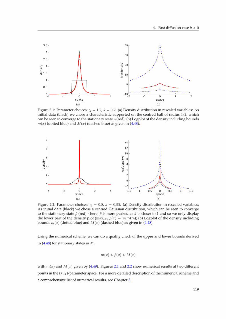
4. Fast diffusion case k ą 0
(a) (b)
Figure 2.1: Parameter choices: χ “ 1.2, k “ 0.2. (a) Density distribution in rescaled variables: Asinitial data (black) we chose a characteristic supported on the centred ball of radius 12, whichcan be seen to converge to the stationary state ρ (red); (b) Logplot of the density including boundsmpxq (dotted blue) andMpxq (dashed blue) as given in (4.48).
(a) (b)
Figure 2.2: Parameter choices: χ “ 0.8, k “ 0.95. (a) Density distribution in rescaled variables:As initial data (black) we chose a centred Gaussian distribution, which can be seen to convergeto the stationary state ρ (red) - here, ρ is more peaked as k is closer to 1 and so we only displaythe lower part of the density plot (maxxPR ρpxq “ 75.7474); (b) Logplot of the density includingboundsmpxq (dotted blue) andMpxq (dashed blue) as given in (4.48).
Using the numerical scheme, we can do a quality check of the upper and lower bounds derived
in (4.48) for stationary states in X :
mpxq ď ρpxq ďMpxq
with mpxq andMpxq given by (4.49). Figures 2.1 and 2.2 show numerical results at two different
points in the pk, χq-parameter space. For a more detailed description of the numerical scheme and
a comprehensive list of numerical results, see Chapter 3.
119
2. Fair-Competition Regime
A Appendix: Properties of ψk
We are here investigating in more detail the properties of the mean-field potential gradient for
global minimisers in the porousmedium regime. Inmore than one dimension, it can be expressed
in terms of hypergeometric functions. Their properties are well understood and allow us to anal-
yse the regularity properties of global minimisers. Since global minimisers of Fk and Fk,resc are
radially symmetric by Proposition 3.6, the aim is here to find the radial formulation of ∇Sk de-
fined in (1.3). In one dimension, explicit expressions are available, and so we are assuming from
now on thatN ě 2. There are three different cases: (1) The Newtonian case k “ 2´N withN ě 3,
(2) the range 1´N ă k ă 0, k ‰ 2´N where ∇pWk ˚ρq is well defined, and (3) the singular range
´N ă k ď 1´N where the force field is given by a Cauchy principle value.
(1) In the Newtonian case k “ 2´N , we have an explicit formula for the radial derivative of the
force field using Newton’s Shell Theorem,
Br pW2´N ˚ ρq prq “Mprqr1´N ,
whereMprq “ σNşr
0 ρpsqsN´1 ds is the mass of ρ in a ball of radius r. Hence, we can write
BrpW2´N ˚ ρqprq “ r1´Nż 8
0ψ2´N
´η
r
¯
ρpηqηN´1 dη
where ψ2´N is defined to have a jump singularity at s “ 1,
ψ2´N psq :“
$
’
&
’
%
1 if 0 ď s ă 1 ,
0 if s ą 1 .(A.54)
(2) In the range 1´N ă k ă 0 and k ‰ 2´N , the mean-field potential gradient is given by
∇Skpxq :“ ∇pWk ˚ ρqpxq “
ż
RN∇W px´ yqρpyqdy
“1σN
ż 8
0
ż
BBp0,|y|q∇W px´ yqdσpyqρp|y|qd|y| .
Denoting |y| “ η, we can write for x “ re1,
1σN
ż
BBp0,|y|q∇W px´ yqdσpyq “ 1
σN
ż
BBp0,|y|qpx´ yq|x´ y|k´2 dσpyq
“
˜
1σN
ż
BBp0,ηqe1 ¨ pre1 ´ yq|re1 ´ y|
k´2 dσpyq¸
x
r
“ ηN´1
˜
1σN
ż
BBp0,1qpr ´ ηe1.zq|re1 ´ ηz|
k´2 dσpzq¸
x
r
“ ηN´1rk´1ψk
´η
r
¯ x
r,
120
A. Appendix: Properties of ψk
where
ψk psq “1σN
ż
BBp0,1qp1´ se1.zq|e1 ´ sz|
k´2 dσpzq , s P r0, 1q Y p1,8q . (A.55)
By radial symmetry,
∇pWk ˚ ρqpxq “ rk´1ˆż 8
0ψk
´η
r
¯
ρpηqηN´1 dη˙
x
r“ BrpWk ˚ ρqprq
x
r
with
BrpWk ˚ ρqprq “ rk´1ż 8
0ψk
´η
r
¯
ρpηqηN´1 dη . (A.56)
(3) In the regime´N ă k ď 1´N however, the derivative of the convolution with the interaction
kernel is a singular integral, and in this case the force field is defined as
∇Sk :“ż
R
x´ y
|x´ y|2´kpρpyq ´ ρpxqq dy
“ limδÑ0
ż
|x´y|ąδ
x´ y
|x´ y|2´kρpyq dy “
x
rBrSkprq
with the radial component given by
BrSkprq “rk´1
ż 8
0ψk
´η
r
¯
pρpηq ´ ρprqq ηN´1 dη
“rk´1 limδÑ0
ż
|r´η|ąδ
ψk
´η
r
¯
ρpηqηN´1 dη ,
and ψk is given by (A.55) on r0, 1q Y p1,8q.
For any ´N ă k ă 0 with k ‰ 2´N , we can rewrite (A.55) as
ψkpsq “σN´1
σN
ż π
0p1´ s cospθqq sinN´2pθqAps, θqk´2 dθ , s P r0, 1q Y p1,8q (A.57)
with
Aps, θq “`
1` s2 ´ 2s cospθq˘12
.
It is useful to express ψk in terms of Gauss Hypergeometric Functions. The hypergeometric func-
tion F pa, b; c; zq is defined as the power series
F pa, b; c; zq “8ÿ
n“0
paqnpbqnpcqn
zn
n! (A.58)
for |z| ă 1 and a, b P C, c P CztZ´ Y t0uu, see [4], where pqqn is the Pochhammer symbol defined
for any q ą 0, n P N by
pqq0 “ 1, pqqn “pn` q ´ 1q!pq ´ 1q! .
We will here make use of its well known integral representation [4]
F pa, b; c; zq “ ΓpcqΓpbqΓpc´ bq
ż 1
0tb´1p1´ tqc´b´1p1´ tzq´a dt
121
2. Fair-Competition Regime
for c ą b ą 0, a ą 0 and |z| ă 1. Moreover, if c ´ a ´ b ą 0, then F is well defined at z “ 1 and
satisfies
F pa, b; c; 1q “ ΓpcqΓpc´ a´ bqΓpc´ aqΓpc´ bq .
Otherwise, we have the limiting case discussed in [4]:
limzÑ1´
F pa, b; c; zqp1´ zqc´a´b “
ΓpcqΓpa` b´ cqΓpaqΓpbq , if c´ a´ b ă 0 . (A.59)
Let us define
Hpa, b; c; zq :“ ΓpbqΓpc´ bqΓpcq F pa, b; c; zq .
To express ψk as a combination of hypergeometric functions, we write
ψkpsq “σN´1
σN
ż π
0p1´ s cospθqq
`
1` s2 ´ 2s cospθq˘
k´22 sinN´2pθq dθ
“σN´1
σNp1` sqk´2
ż π
0p1´ s cospθqq
ˆ
1´ 4sp1` sq2 cos2
ˆ
θ
2
˙˙
k´22
sinN´2 pθq dθ
“σN´1
σNp1` sqk´2
ż π
0
ˆ
1´ 4sp1` sq2 cos2
ˆ
θ
2
˙˙
k´22
sinN´2 pθq dθ
´σN´1
σNp1` sqk´2
s
ż π
0cospθq
ˆ
1´ 4sp1` sq2 cos2
ˆ
θ
2
˙˙
k´22
sinN´2 pθq dθ
“:f1psq ´ f2psq .
Now, we use the change of variable t “ cos2 pθ2q to get
f1psq “σN´1
σNp1` sqk´2
ż π
0
ˆ
1´ 4sp1` sq2 cos2
ˆ
θ
2
˙˙
k´22
sinN´2 pθq dθ
“σN´1
σNp1` sqk´2 2N´2
ż 1
0
ˆ
1´ 4sp1` sq2 t
˙
k´22
tN´3
2 p1´ tqN´3
2 dt
“σN´1
σNp1` sqk´2 2N´2H pa, b1; c1; zq
with
a :“ 1´ k
2 , b1 :“ N ´ 12 , c1 :“ N ´ 1, z :“ 4s
p1` sq2 .
Let us define h1psq :“ f1psq, and
h2psq :“ σN´1
σNp1` sqk´2 2N´2H pa, b2; c2; zq
with
a :“ 1´ k
2 , b2 :“ N ´ 12 , c2 :“ N ´ 1, z :“ 4s
p1` sq2 .
Then
f2psq “σN´1
σNp1` sqk´2
s
ż π
0cospθq
ˆ
1´ 4sp1` sq2 cos2
ˆ
θ
2
˙˙
k´22
sinN´2 pθq dθ
“´ sh1psq ` 2sh2psq
122
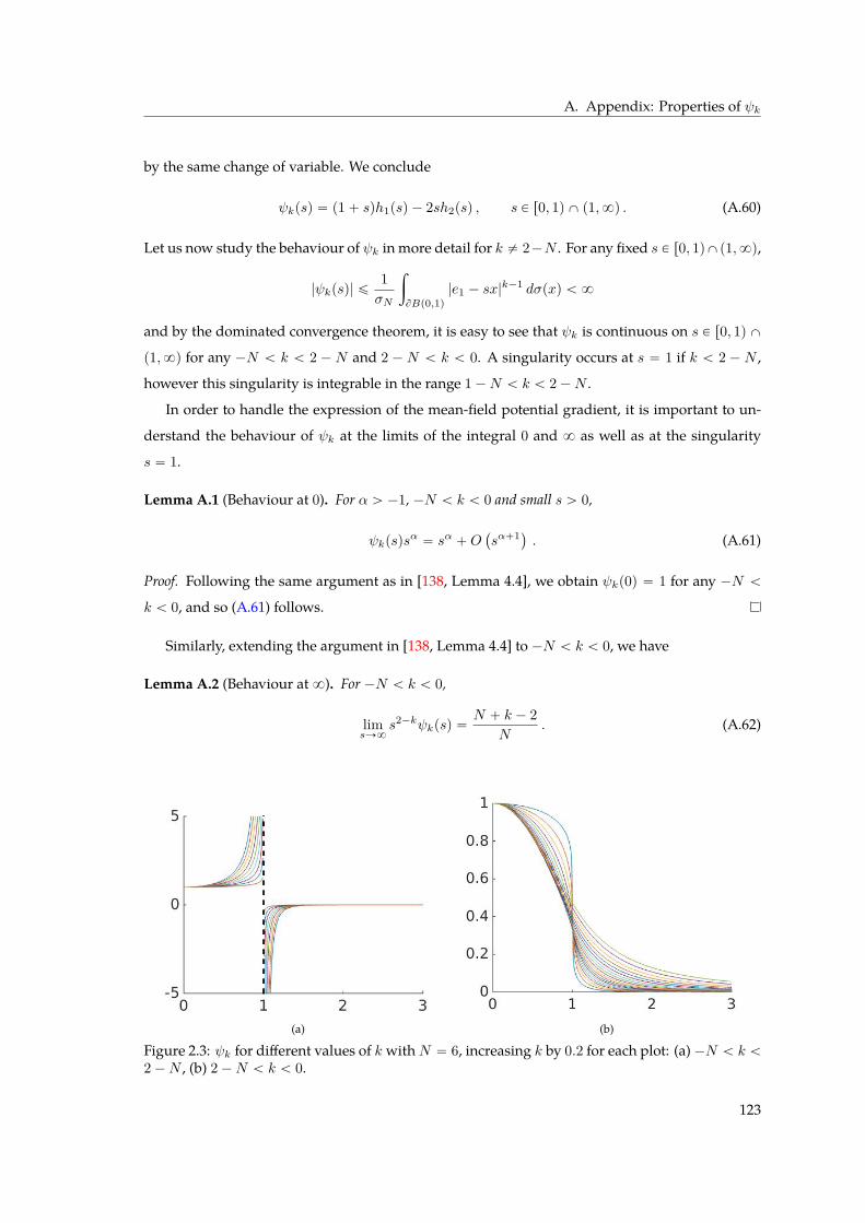
A. Appendix: Properties of ψk
by the same change of variable. We conclude
ψkpsq “ p1` sqh1psq ´ 2sh2psq , s P r0, 1q X p1,8q . (A.60)
Let us now study the behaviour of ψk in more detail for k ‰ 2´N . For any fixed s P r0, 1qXp1,8q,
|ψkpsq| ď1σN
ż
BBp0,1q|e1 ´ sx|
k´1 dσpxq ă 8
and by the dominated convergence theorem, it is easy to see that ψk is continuous on s P r0, 1q X
p1,8q for any ´N ă k ă 2 ´ N and 2 ´ N ă k ă 0. A singularity occurs at s “ 1 if k ă 2 ´ N ,
however this singularity is integrable in the range 1´N ă k ă 2´N .
In order to handle the expression of the mean-field potential gradient, it is important to un-
derstand the behaviour of ψk at the limits of the integral 0 and 8 as well as at the singularity
s “ 1.
Lemma A.1 (Behaviour at 0). For α ą ´1, ´N ă k ă 0 and small s ą 0,
ψkpsqsα “ sα `O
`
sα`1˘ . (A.61)
Proof. Following the same argument as in [138, Lemma 4.4], we obtain ψkp0q “ 1 for any ´N ă
k ă 0, and so (A.61) follows.
Similarly, extending the argument in [138, Lemma 4.4] to ´N ă k ă 0, we have
Lemma A.2 (Behaviour at8). For ´N ă k ă 0,
limsÑ8
s2´kψkpsq “N ` k ´ 2
N. (A.62)
(a) (b)
Figure 2.3: ψk for different values of k withN “ 6, increasing k by 0.2 for each plot: (a)´N ă k ă2´N , (b) 2´N ă k ă 0.
123
2. Fair-Competition Regime
Further, it is obvious from (A.57) that ψkpsq ą 0 for s P p0, 1q. From [138],
ψ1kpsq “
ˆ
σN´1
σN
˙
pk ´ 2qpN ` k ´ 2qpN ´ 1q s
ż π
0sinN pθqAps, θqk´4 dθ , s P r0, 1q X p1,8q
andhenceψk is strictly decreasing for k ą 2´N and strictly increasing for k ă 2´N . It then follows
from (A.62) that in the super-Newtonian regime k ą 2 ´ N , ψk converges to zero as s Ñ 8, is
finite and continuous at s “ 1, and strictly positive on r0,8q (Figure 2.3(b)). In the sub-Newtonian
regime´N ă k ă 2´N on the other hand, the monotonicity of ψk and the fact that ψk converges
to 0 as sÑ8 imply that
limsÑ1´
ψkpsq “ `8 , limsÑ1`
ψkpsq “ ´8 ,
and so we conclude that ψk ă 0 on p1,8q if´N ă k ă 2´N (Figure 2.3(a)). We summarise these
observations in the following lemma:
Lemma A.3 (Overall Behaviour). Let ψk be as defined in (A.55).
(i) If 2´N ă k ă 0, then ψk is continuous, positive and strictly decreasing on r0,8q.
(ii) If ´N ă k ă 2 ´ N , then ψk is continuous, positive and strictly increasing on r0, 1q, and it is
continuous, negative and strictly increasing on p1,8q. Further, it has a singularity at s “ 1 which is
integrable for 1´N ă k ă 2´N .
Using the hypergeometric function representation ofψk, we can characterise its behaviour near
the singularity.
Lemma A.4 (Behaviour at 1). For α P R and ε ą 0 small, we have
(1) in the super-Newtonian regime 2´N ă k ă 0 and for s “ 1˘ ε:
ψkpsqsα “ ψkp1q `O pεq ,
(2) in the sub-Newtonian regime ´N ă k ă 2´N and
(i) for s “ 1´ ε:
ψk psq sα “ K1ε
N`k´2 `K2εN`k´1 `O
`
εN`k˘
, (A.63)
(ii) for s “ 1` ε:
ψk psq sα “ ´K1ε
N`k´2 `K3εN`k´1 `O
`
εN`k˘
, (A.64)
124
A. Appendix: Properties of ψk
where
K1 “
ˆ
σN´1
σN
˙
γ
2 ą 0 , K2rαs “ ´
ˆ
σN´1
σN
˙ˆ
B1 ` γp1´N ` 2αq4
˙
, (A.65)
K3rαs “ ´
ˆ
σN´1
σN
˙ˆ
B1 ` γp2k `N ´ 5` 2αq4
˙
and
γ “Γpc2 ´ b2qΓpa` b2 ´ c2q
Γpaq ą 0 . (A.66)
Proof. (1) follows directly from the fact that ψk is continuous at s “ 1 [138, Lemma 4.4]. In order
to prove (2), we make use of expression (A.60) for ψk in terms of hypergeometric functions and
known expansions around the point of singularity. Denoting δ :“ ε|2 ´ ε| ą 0, we have for any
β ą 0,
δβ “´ε
2
¯β
` β´ε
2
¯β`1`O
`
εβ`2˘ . (A.67)
From (A.60) we can write
ψkpsq “ p1` sqh1psq ´ 2sh2psq “ p1` sq ph1psq ´ h2psqq ` p1´ sqh2psq ,
and hence, denoting z “ 1´ δ2, we obtain for s “ 1´ ε:
22´N σNσN´1
ψkp1´ εq “ p2´ εqk´1pH pa, b1; c1; zq ´H pa, b2; c2; zqq
` ε p2´ εqk´2H pa, b2; c2; zq
“ p2´ εqk´1δN`k´3
ˆ
H pa, b1; c1; zqp1´ zqc1´a´b1
´H pa, b2; c2; zqp1´ zqc2´a´b2
˙
` ε p2´ εqk´2δN`k´3
ˆ
H pa, b2; c2; zqp1´ zqc2´a´b2
˙
. (A.68)
Similarly, above the singularity point at s “ 1` ε, we obtain:
22´N σNσN´1
ψkp1` εq “ p2` εqk´1δN`k´3
ˆ
H pa, b1; c1; zqp1´ zqc1´a´b1
´H pa, b2; c2; zqp1´ zqc2´a´b2
˙
´ ε p2` εqk´2δN`k´3
ˆ
H pa, b2; c2; zqp1´ zqc2´a´b2
˙
. (A.69)
Using the power series expression (A.58) for hypergeometric functions, we can writeˆ
H pa, b1; c1; zqp1´ zqc1´a´b1
´H pa, b2; c2; zqp1´ zqc2´a´b2
˙
“
8ÿ
n“0An
zn
n! “8ÿ
m“0
p´1qmBmm! δ2m ,
Bm :“8ÿ
n“m
Anpn´mq! ,
An :“ˆ
pc1 ´ aqnpc1 ´ b1qnpc1qn
´ b1pc2 ´ aqnpc2 ´ b2qn
pc2qn
˙
Γpb1qΓpc1 ´ b1qΓpaq .
In the singularity regime ´N ă k ă 2´N , we have
c1 ´ a´ b1 “ c2 ´ a´ b2 “N ` k ´ 3
2 ă 0 ,
125
2. Fair-Competition Regime
and so we can make use of (A.59) to show that the leading order term vanishes:
B0 “ limδÑ0
8ÿ
m“0
p´1qmBmm! δ2m “ lim
zÑ1´
ˆ
H pa, b1; c1; zqp1´ zqc1´a´b1
´H pa, b2; c2; zqp1´ zqc2´a´b2
˙
“Γpc1 ´ b1qΓpa` b1 ´ c1q
Γpaq ´Γpc2 ´ b2qΓpa` b2 ´ c2q
Γpaq “ 0 .
Hence
H pa, b1; c1; zqp1´ zqc1´a´b1
´H pa, b2; c2; zqp1´ zqc2´a´b2
“ ´B1δ2 `Opδ4q ,
H pa, b2; c2; zqp1´ zqc2´a´b2
“Γpc2 ´ b2qΓpa` b2 ´ c2q
Γpaq `O`
δ2˘ :“ γ `O`
δ2˘ .
Substituting these estimates and making use of (A.67), (A.68) becomes
22´N σNσN´1
ψkp1´ εq “ ε p2´ εqk´2 `γδN`k´3 `O
`
δN`k´1˘˘ ,
` p2´ εqk´1 `´B1δ
N`k´1 `O`
δN`k`1˘˘
“ ε“
2k´2 ´ εpk ´ 2q2k´3 `O`
ε2˘‰
ˆ
„
γ´ε
2
¯N`k´3` γ pN ` k ´ 3q
´ε
2
¯N`k´2`O
`
εN`k´1˘
`“
2k´1 `O pεq‰
„
´B1
´ε
2
¯N`k´1`O
`
εN`k˘
“ γ2´N`1εN`k´2 ` γ2´N rpN ` k ´ 3q ` p2´ kqs εN`k´1
´B12´NεN`k´1 `O`
εN`k˘
“ γ2´N`1εN`k´2 ` 2´N rγ pN ´ 1q ´B1s εN`k´1 `O
`
εN`k˘
.
Similarly, (A.69) has expansion
22´N σNσN´1
ψkp1` εq “ ´ ε p2` εqk´2 `γδN`k´3 `O
`
δN`k´1˘˘ ,
` p2` εqk´1 `´B1δ
N`k´1 `O`
δN`k`1˘˘
“ ´ ε“
2k´2 ` εpk ´ 2q2k´3 `O`
ε2˘‰
ˆ
„
γ´ε
2
¯N`k´3` γ pN ` k ´ 3q
´ε
2
¯N`k´2`O
`
εN`k´1˘
`“
2k´1 `O pεq‰
„
´B1
´ε
2
¯N`k´1`O
`
εN`k˘
“ ´ γ2´N`1εN`k´2 ` γ2´N r´ pN ` k ´ 3q ` p2´ kqs εN`k´1
´B12´NεN`k´1 `O`
εN`k˘
“ ´ γ2´N`1εN`k´2 ` 2´N rγ p5´N ´ 2kq ´B1s εN`k´1 `O
`
εN`k˘
.
126
A. Appendix: Properties of ψk
We conclude
ψkp1´ εq “ˆ
σN´1
σN
˙
´γ
2
¯
εN`k´2 `
ˆ
σN´1
σN
˙ˆ
γ pN ´ 1q ´B1
4
˙
εN`k´1 `O`
εN`k˘
,
ψkp1` εq “ ´ˆ
σN´1
σN
˙
´γ
2
¯
εN`k´2 `
ˆ
σN´1
σN
˙ˆ
γ p5´N ´ 2kq ´B1
4
˙
εN`k´1 `O`
εN`k˘
,
and so (2)(i)-(ii) directly follow.
127

Chapter3
Asymptotics in the One-Dimensional
Fair-Competition Regime
This chapter follows in most parts the article “The geometry of diffusing and self-attracting parti-
cles in a one-dimensional fair-competition regime” written in collaboration with Vincent Calvez1
and José A. Carrillo2, and to appear in “Nonlocal and Nonlinear Diffusions and Interactions: New
Methods and Directions”, volume 2186 of Lecture Notes in Math., Springer.
Chapter Summary
We consider an aggregation-diffusion equation modelling particle interaction with non-
linear diffusion and non-local attractive interaction using a homogeneous kernel (singular and
non-singular) leading to variants of the Keller–Segel model of chemotaxis. We analyse the fair-
competition regime in which both homogeneities scale the same with respect to dilations. Our
analysis here deals with the one-dimensional case, building on the work in Chapter 2, and pro-
vides an almost complete classification. In the singular kernel case and for critical interaction
strength, we prove uniqueness of stationary states via a variant of theHardy-Littlewood-Sobolev
inequality. Using the same methods, we show uniqueness of self-similar profiles in the sub-
critical case by proving a new type of functional inequality. Surprisingly, the same results hold
true for any interaction strength in the non-singular kernel case. Further, we investigate the
asymptotic behaviour of solutions, proving convergence to equilibrium in Wasserstein distance
in the critical singular kernel case, and convergence to self-similarity for sub-critical interaction
strength, both under a uniform stability condition. Moreover, solutions converge to a unique
self-similar profile in the non-singular kernel case. Finally, we provide a numerical overview
for the asymptotic behaviour of solutions in the full parameter space demonstrating the above
results. We also discuss a number of phenomena appearing in the numerical explorations for
the diffusion-dominated and attraction-dominated regimes.
1Unité de Mathématiques Pures et Appliquées, CNRS UMR 5669 and équipe-projet INRIA NUMED, École NormaleSupérieure de Lyon, Lyon, France.
2Department of Mathematics, Imperial College London, South Kensington Campus, London SW7 2AZ, UK.
129
3. 1D Fair-Competition Regime
Chapter Content
1 Introduction . . . . . . . . . . . . . . . . . . . . . . . . . . . . . . . . . . . . . . . 131
2 Preliminaries . . . . . . . . . . . . . . . . . . . . . . . . . . . . . . . . . . . . . . 136
2.1 Stationary states: definition & basic properties . . . . . . . . . . . . . . . 136
2.2 Overview of results in the fair-competition regime . . . . . . . . . . . . 138
2.3 Optimal transport tools . . . . . . . . . . . . . . . . . . . . . . . . . . . . 141
3 Functional inequalities . . . . . . . . . . . . . . . . . . . . . . . . . . . . . . . . . 142
3.1 Porous medium case k ă 0 . . . . . . . . . . . . . . . . . . . . . . . . . . 143
3.2 Fast diffusion case k ą 0 . . . . . . . . . . . . . . . . . . . . . . . . . . . 150
4 Long-time asymptotics . . . . . . . . . . . . . . . . . . . . . . . . . . . . . . . . . 153
4.1 Porous medium asymptotics . . . . . . . . . . . . . . . . . . . . . . . . . 154
4.2 Fast diffusion asymptotics . . . . . . . . . . . . . . . . . . . . . . . . . . 167
5 Numerical simulations . . . . . . . . . . . . . . . . . . . . . . . . . . . . . . . . . 169
5.1 Numerical scheme . . . . . . . . . . . . . . . . . . . . . . . . . . . . . . . 170
5.2 Results . . . . . . . . . . . . . . . . . . . . . . . . . . . . . . . . . . . . . 171
6 Explorations in other regimes . . . . . . . . . . . . . . . . . . . . . . . . . . . . . 182
6.1 Diffusion-dominated regime in one dimension . . . . . . . . . . . . . . 182
6.2 Attraction-dominated regime in any dimension . . . . . . . . . . . . . . 182
Ati deka metua xo o.
One stick cannot build a house3.
Ghanaian proverb (Ewe)
3In unity is strength, therefore, one should learn to work together with others.
130
1. Introduction
1 Introduction
Mean field macroscopic models for interacting particle systems have been derived in the liter-
ature [245, 240] with the objective of explaining the large time behaviour, the qualitative prop-
erties and the stabilisation of systems composed by a large number of particles with compet-
ing effects such as repulsion and attraction between particles. They find natural applications in
mathematical biology, gravitational collapse, granular media and self-assembly of nanoparticles,
see [105, 196, 96, 282, 191, 207] and the references therein. These basic models start from particle
dynamics in which their interaction is modelled via pairwise potentials. By assuming the right
scaling between the typical interaction length and the number of particles per unit area one can
obtain different mean field equations, see for instance [43]. In the mean-field scaling they lead
to non-local equations with velocity fields obtained as an average force from a macroscopic den-
sity encoding both repulsion and attraction, see [39, 10] and the references therein. However, if
the repulsion strength is very large at the origin, one can model repulsive effects by (non-linear)
diffusion while attraction is considered via non-local long-range forces [240, 282].
In this chapter, we concentrate on this last approximation: repulsion is modelled by diffusion
and attraction by non-local forces. We will make a survey of the main results in this topic exem-
plifying them in the one dimensional setting while at the same time we will provide newmaterial
in one dimension with alternative proofs and information about long time asymptotics which are
not known yet in higher dimensions. In order to understand the interplay between repulsion via
non-linear diffusion and attraction via non-local forces, we concentrate on the simplest possible
situation in which both the diffusion and the non-local attractive potential are homogeneous func-
tions. We will focus on models with a variational structure that dissipate the free energy of the
system.
The plan for this chapter is twofold. In a first part we shall investigate some properties of
the following class of homogeneous functionals, defined for centered probability densities ρpxq,
belonging to suitable weighted Lp-spaces, and some interaction strength coefficient χ ą 0 and
diffusion powerm ą 0:
Fm,krρs “ż
RUm pρpxqq dx` χ
ij
RˆR
ρpxqWkpx´ yqρpyq dxdy :“ Umrρs ` χWkrρs , (1.1)
ρpxq ě 0 ,ż
Rρpxq dx “ 1 ,
ż
Rxρpxq dx “ 0 ,
with
Umpρq “
$
’
&
’
%
1m´ 1 ρ
m , if m ‰ 1
ρ log ρ , if m “ 1,
131
3. 1D Fair-Competition Regime
and
Wkpxq “
$
’
&
’
%
|x|k
k, if k P p´1, 1qzt0u
log |x| , if k “ 0. (1.2)
The center of mass of the density ρ is assumed to be zero since the free energy functional is invari-
ant by translation. Taking mass preserving dilations, one can see that Umr¨s scales with a power
m ´ 1, whilst Wkr¨s scales with power ´k, indicating that the relation between the parameters k
andm plays a crucial role here. And indeed, one observes different types of behaviour depending
on which of the two forces dominates, non-linear diffusion or non-local attraction. This motivates
the definition of three different regimes: the diffusion-dominated regime (m ´ 1 ą ´k), the fair-
competition regime (m ´ 1 “ ´k), and the attraction-dominated regime (m ´ 1 ă ´k). We will here
concentrate mostly on the fair-competition regime.
This chapter can be viewed as a continuation of the seminal paper by McCann [234] in a non-
convex setting. Indeed, McCann used the very powerful toolbox of Euclidean optimal transporta-
tion to analyse functionals like (1.1) in the casem ě 0 and for a convex interaction kernelWk. He
discovered that such functionals are equipped with an underlying convexity structure, for which
the interpolant rρ0, ρ1st follows the line of optimal transportation [295]. This provides many in-
teresting features among which a natural framework to show uniqueness of the ground state as
soon as it exists. In this chapter we deal with concave homogeneous interaction kernelsWk given
by (1.2) for which McCann’s results [234] do not apply. Actually, the conditions on k imply that
the interaction kernelWk is locally integrable on R and concave on R`, which means that Wkr¨s is
displacement concave as shown in [85]. We explain in this chapter how some ideas from [234] can
be extended to some convex-concave competing effects. Our main statement is that the functional
(1.1) – the sum of a convex and a concave functional – behaves almost like a convex functional
in some good cases detailed below. In particular, existence of a critical point implies uniqueness
(up to translations and dilations). The bad functional contribution is somehow absorbed by the
convex part for certain homogeneity relations and parameters χ.
The analysis of these free energy functionals and their respective gradient flows is closely re-
lated to some functional inequalities of Hardy-Littlewood-Sobolev (HLS) type [218, 163, 74, 39].
To give a flavour, we highlight the case pm “ 1, k “ 0q, called the logarithmic case. It is known
from [136, 41] using [77, 19] that the functionalF1,0 is bounded frombelow if and only if 0 ă χ ď 1.
Moreover, F1,0 achieves its minimum if and only if χ “ 1 and the extremal functions are mass-
preserving dilations of Cauchy’s density:
ρ0pxq “1π
ˆ
11` |x|2
˙
. (1.3)
132
1. Introduction
In [77] authors have proved the uniqueness (up to dilations and translations) of this logarithmic
HLS inequality based on a competing-symmetries argument. We develop in this chapter an alter-
native argument based on some accurate use of the Jensen’s inequality to get similar results in the
porous medium case ´1 ă k ă 0. This goal will be achieved for some variant of the HLS inequal-
ity as in [39], indeed being a combination of the HLS inequality and interpolation estimates, see
Theorem 3.1. The case 0 ă k ă 1 has been a lot less studied, and we will show here that no crit-
ical interaction strength exists as there is no χ ą 0 for which Fm,k admits global minimisers. On
the other hand, we observe certain similarities with the behaviour of the fast diffusion equation
(0 ă m ă 1, χ “ 0) [287]. The mass-preserving dilation homogeneity of the functional Fm,k is
shared by the range of parameters pm, kq with Npm ´ 1q ` k “ 0 for all dimensions, m ą 0 and
k P p´N,Nq. This general fair-competition regime is analysed in Chapter 2.
In a second stage, here we also tackle the behaviour of the following family of partial differen-
tial equations modelling self-attracting diffusive particles at the macroscopic scale,$
&
%
Btρ “ Bxx pρmq ` 2χBx pρ BxSkq , t ą 0 , x P R ,
ρpt “ 0, xq “ ρ0pxq .(1.4)
where we define the mean-field potential Skpxq :“ Wkpxq ˚ ρpxq. For k ą 0, the gradient BxSk :“
Bx pWk ˚ ρq is well defined. For k ă 0 however, it becomes a singular integral, and we thus define
it via a Cauchy principal value. Hence, the mean-field potential gradient in equation (1.4) is given
by
BxSkpxq :“
$
’
’
&
’
’
%
BxWk ˚ ρ , if 0 ă k ă 1 ,ż
RBxWkpx´ yq pρpyq ´ ρpxqq dy , if ´ 1 ă k ă 0 .
(1.5)
Further, it is straightforward to check that equation (1.4) formally preserves positivity, mass and
centre of mass, and so we can choose to impose
ρ0pxq ě 0 ,ż
ρ0pxq dx “ 1 ,ż
xρ0pxq dx “ 0 .
This class of PDEs are one of the prime examples for competition between the diffusion (possibly
non-linear), and the non-local, quadratic non-linearity which is due to the self-attraction of the
particles through the mean-field potential Skpxq. The parameter χ ą 0 measures the strength of
the interaction. We would like to point out that we are here not concerned with the regularity of
solutions or existence/uniqueness results for equation (1.4), allowing ourselves to assume solu-
tions are ’nice’ enough in space and time for our analysis to hold (for more details on regularity
assumptions, see Section 4).
133
3. 1D Fair-Competition Regime
There exists a strong link between the PDE (1.4) and the functional (1.1). Not only is Fm,kdecreasing along the trajectories of the system, but more importantly, system (1.4) is the formal
gradient flow of the free energy functional (1.1) when the space of probability measures is en-
dowed with the Euclidean Wasserstein metric W:
Btρptq “ ´∇WFm,krρptqs . (1.6)
This illuminating statement has been clarified in the seminal paper by Otto [248]. We also refer
to the books by Villani [295] and Ambrosio, Gigli and Savaré [3] for a comprehensive presenta-
tion of this theory of gradient flows in Wasserstein metric spaces, particularly in the convex case.
Performing gradient flows of a convex functional is a natural task, and suitable estimates from
below on the Hessian of Fm,k in (1.1) translate into a rate of convergence towards equilibrium for
the PDE [96, 295, 97]. However, performing gradient flow of functionals with convex and concave
contributions is more delicate, and one has to seek compensations. Such compensations do exist
in our case, and one can prove convergence in Wasserstein distance towards some stationary state
under suitable assumptions, in some cases with an explicit rate of convergence. It is of course
extremely important to understand how the convex and the concave contributions are entangled.
The results obtained in the fully convex case generally consider each contribution separately,
resp. internal energy, potential confinement energy or interaction energy, see [96, 295, 3, 97]. It
happens however that adding two contributions provides better convexity estimates. In [96] for
instance the authors prove exponential speed of convergence towards equilibrium when a degen-
erate convex potentialWk is coupled with strong enough diffusion, see [44] for improvements.
The family of non-local PDEs (1.4) has been intensively studied in various contexts arising in
physics and biology. The two-dimensional logarithmic case pm “ 1, k “ 0q is the so-called Keller–
Segel system in its simplest formulation [196, 197, 243, 194, 41, 256]. It has been proposed as a
model for chemotaxis in cell populations. The three-dimensional configuration pm “ 1, k “ ´1q
is the so-called Smoluchowski-Poisson system arising in gravitational physics [105, 107, 106]. It
describes macroscopically a density of particles subject to a self-sustained gravitational field.
Let us describe in more details the two-dimensional Keller–Segel system, as the analysis of its
peculiar structure will serve as a guideline to understand other cases. The corresponding gradient
flow is subject to a remarkable dichotomy, see [113, 194, 242, 159, 136, 41] . The density exists
globally in time if χ ă 1 (diffusion overcomes self-attraction), whereas blow-up occurs in finite
timewhen χ ą 1 (self-attraction overwhelms diffusion). In the sub-critical case, it has been proved
that solutions decay to self-similarity solutions exponentially fast in suitable rescaled variables [70,
71, 148]. In the super-critical case, solutions blow-up in finite time with by nowwell studied blow-
up profiles for close enough to critical cases, see [187, 260].
134
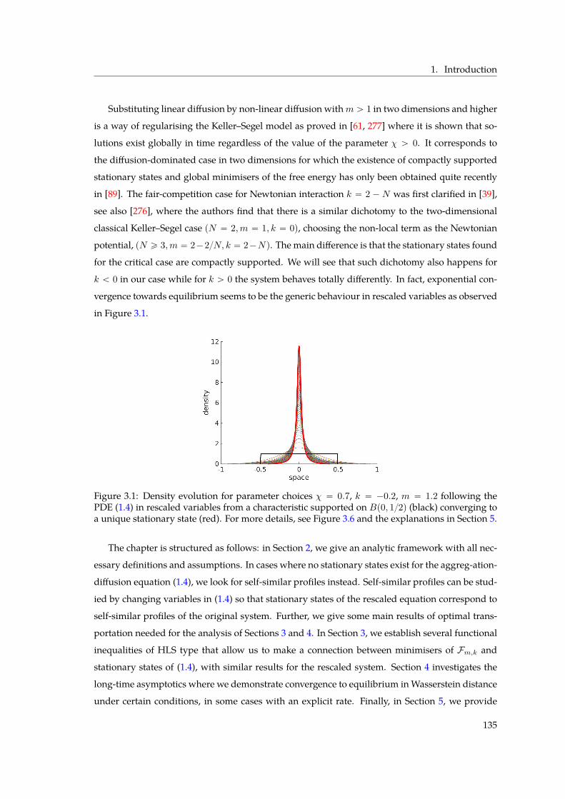
1. Introduction
Substituting linear diffusion by non-linear diffusion withm ą 1 in two dimensions and higher
is a way of regularising the Keller–Segel model as proved in [61, 277] where it is shown that so-
lutions exist globally in time regardless of the value of the parameter χ ą 0. It corresponds to
the diffusion-dominated case in two dimensions for which the existence of compactly supported
stationary states and global minimisers of the free energy has only been obtained quite recently
in [89]. The fair-competition case for Newtonian interaction k “ 2 ´ N was first clarified in [39],
see also [276], where the authors find that there is a similar dichotomy to the two-dimensional
classical Keller–Segel case pN “ 2,m “ 1, k “ 0q, choosing the non-local term as the Newtonian
potential, pN ě 3,m “ 2´2N, k “ 2´Nq. The main difference is that the stationary states found
for the critical case are compactly supported. We will see that such dichotomy also happens for
k ă 0 in our case while for k ą 0 the system behaves totally differently. In fact, exponential con-
vergence towards equilibrium seems to be the generic behaviour in rescaled variables as observed
in Figure 3.1.
Figure 3.1: Density evolution for parameter choices χ “ 0.7, k “ ´0.2, m “ 1.2 following thePDE (1.4) in rescaled variables from a characteristic supported on Bp0, 12q (black) converging toa unique stationary state (red). For more details, see Figure 3.6 and the explanations in Section 5.
The chapter is structured as follows: in Section 2, we give an analytic framework with all nec-
essary definitions and assumptions. In cases where no stationary states exist for the aggreg-ation-
diffusion equation (1.4), we look for self-similar profiles instead. Self-similar profiles can be stud-
ied by changing variables in (1.4) so that stationary states of the rescaled equation correspond to
self-similar profiles of the original system. Further, we give some main results of optimal trans-
portation needed for the analysis of Sections 3 and 4. In Section 3, we establish several functional
inequalities of HLS type that allow us to make a connection between minimisers of Fm,k and
stationary states of (1.4), with similar results for the rescaled system. Section 4 investigates the
long-time asymptotics where we demonstrate convergence to equilibrium inWasserstein distance
under certain conditions, in some cases with an explicit rate. Finally, in Section 5, we provide
135
3. 1D Fair-Competition Regime
numerical simulations of system (1.4) to illustrate the properties of equilibria and self-similar pro-
files in the different parameter regimes for the fair-competition regime. In Section 6, we use the
numerical scheme to explore the asymptotic behaviour of solutions in the diffusion- and attraction-
dominated regimes.
2 Preliminaries
2.1 Stationary states: definition & basic properties
Let us define precisely the notion of stationary states to the aggregation-diffusion equation (1.4).
Definition 2.1. Given ρ P L1` pRq X L8 pRq with ||ρ||1 “ 1, it is a stationary state for the evolution
equation (1.4) if ρm P W1,2loc pRq, BxSk P L1
loc pRq, and it satisfies
Bxρm “ ´2χ ρBxSk
in the sense of distributions in R. If k P p´1, 0q, we further require ρ P C0,α pRq with α P p´k, 1q.
In fact, the function Sk and its gradient defined in (1.5) satisfy even more than the regularity
BxSk P L1loc pRq required in Definition 2.1. We have from Chapter 2 Lemma 2.2:
Lemma 2.2. Let ρ P L1` pRq X L8 pRq with ||ρ||1 “ 1. If k P p0, 1q, we additionally assume |x|kρ P
L1 pRq. Then the following regularity properties hold:
i) Sk P L8loc pRq for 0 ă k ă 1 and Sk P L8 pRq for ´1 ă k ă 0.
ii) BxSk P L8 pRq for k P p´1, 1qzt0u, assuming additionally ρ P C0,α pRq with α P p´k, 1q in the
range ´1 ă k ă 0.
Furthermore, for certain cases, see Chapter 2, there are no stationary states to (1.4) in the sense
of Definition 2.1 (for a dynamical proof of this fact, see Remark 4.6 in Section 4.1.2), and so the
scale invariance of (1.4) motivates us to look for self-similar solutions instead. To this end, we
rescale equation (1.4) to a non-linear Fokker–Planck type equation as in [100]. Let us define
upt, xq :“ αptqρ pβptq, αptqxq ,
where ρpt, xq solves (1.4) and the functions αptq, βptq are to be determined. If we assume up0, xq “
ρp0, xq, then upt, xq satisfies the rescaled drift-diffusion equation$
’
&
’
%
Btu “ Bxxum ` 2χBx pu BxSkq ` Bx pxuq , t ą 0 , x P R ,
upt “ 0, xq “ ρ0pxq ě 0 ,ż 8
´8
ρ0pxq dx “ 1 ,ż 8
´8
xρ0pxq dx “ 0 ,(2.7)
136
2. Preliminaries
for the choices
αptq “ et, βptq “
$
’
&
’
%
12´k
`
ep2´kqt ´ 1˘
, if k ‰ 2 ,
t, if k “ 2 ,(2.8)
and with BxSk given by (1.5) with u instead of ρ. By differentiating the centre of mass of u, we see
easily thatż
Rxupt, xq dx “ e´t
ż
Rxρ0pxq dx “ 0 , @t ą 0 ,
and so the initial zero centre of mass is preserved for all times. Self-similar solutions to (1.4) now
correspond to stationary solutions of (2.7). Similar to Definition 2.1, we state what we exactly
mean by stationary states to the aggregation-diffusion equation (2.7).
Definition 2.3. Given u P L1` pRq X L8 pRq with ||u||1 “ 1, it is a stationary state for the evolution
equation (2.7) if um P W1,2loc pRq, BxSk P L1
loc pRq, and it satisfies
Bxum “ ´2χ uBxSk ´ x u
in the sense of distributions in R. If ´1 ă k ă 0, we further require u P C0,α pRq with α P p´k, 1q.
From now on, we switch notation from u to ρ for simplicity, it should be clear from the context
if we are in original or rescaled variables. In fact, stationary states as defined above have even
more regularity:
Lemma 2.4. Let k P p´1, 1qzt0u and χ ą 0.
(i) If ρ is a stationary state of equation (1.4) with |x|kρ P L1 pRq in the case 0 ă k ă 1, then ρ is
continuous on R.
(ii) If ρresc is a stationary state of equation (2.7) with |x|kρresc P L1 pRq in the case 0 ă k ă 1, then ρrescis continuous on R.
In the case k ă 0, we furthermore have a non-linear algebraic equation for stationary states as
shown in Chapter 2 Corollary 2.5:
Corollary 2.5 (Necessary Condition for Stationary States). Let k P p´1, 0q and χ ą 0.
(i) If ρ is a stationary state of equation (1.4), then ρ P W1,8 pRq and it satisfies
ρpxqm´1 “pm´ 1qm
`
Ckrρspxq ´ 2χ Skpxq˘
`, @x P R ,
where Ckrρspxq is constant on each connected component of supp pρq.
(ii) If ρresc is a stationary state of equation (2.7), then ρresc P W1,8loc pRq and it satisfies
ρrescpxqm´1 “
pm´ 1qm
ˆ
Ck,rescrρspxq ´ 2χ Skpxq ´|x|2
2
˙
`
, @x P R ,
where Ck,rescrρspxq is constant on each connected component of supp pρrescq.
137
3. 1D Fair-Competition Regime
2.2 Overview of results in the fair-competition regime
It is worth noting that the functional Fm,krρs possesses remarkable homogeneity properties, see
Chapter 1 Section 3.1. We will here only concentrate on the one-dimensional fair-competition
regime m ` k “ 1, and denote the corresponding energy functional by Fkrρs “ F1´k,krρs. For a
definition of the different regimes and detailed explanations and references, see Chapter 1 Defini-
tion 3.1. An overview of the parameter space pk,mq and the different regimes is given in Chapter
1 Figure 1.4. Notice that the functional Fk is homogeneous in the fair-competition regime, i.e.,
Fkrρλs “ λ´kFkrρs .
In this chapter, we wil first do a review of the main results known in one dimension about the sta-
tionary states and minimisers of the aggregation-diffusion equation in the fair-competition case.
The novelties will be showing the functional inequalities independently of the flow and studying
the long-time asymptotics of the equations (1.4) and (2.7) by exploiting the one dimensional set-
ting. The analysis in the fair-competition regime depends on the sign of k, see Chapter 1 Definition
3.7, andwe therefore split our investigations into the porousmedium case (k ă 0), and the fast dif-
fusion case (k ą 0). More information on the logarithmic case (k “ 0) can be found in [62]. When
dealing with the energy functional Fk, we work in the set of non-negative normalised densities,
Y :“"
ρ P L1` pRq X Lm pRq : ||ρ||1 “ 1 ,
ż
xρpxq dx “ 0*
.
In rescaled variables, equation (2.7) is the formal gradient flow of the rescaled free energy func-
tional Fk,resc, which is complemented with an additional quadratic confinement potential,
Fk,rescrρs “ Fkrρs `12Vrρs , Vrρs “
ż
R|x|2ρpxq dx .
Defining the set Y2 :“ tρ P Y : Vrρs ă 8u, we see that Fk,resc is well-defined and finite on Y2.
Thanks to the formal gradient flow structure in the EuclideanWasserstein metricW, we can write
the rescaled equation (2.7) as
Btρ “ ´∇WFk,rescrρs .
In what follows, we will make use of a different characterisation of stationary states based on
some integral reformulation of the necessary condition stated in Corollary 2.5. This characterisa-
tion was also the key idea in [62] to improve on the knowledge of the asymptotic stability of steady
states and the functional inequalities behind.
Lemma 2.6 (Characterisation of stationary states). Let k P p´1, 1qzt0u,m “ 1´ k and χ ą 0.
(i) Any stationary state ρk P Y of system (1.4) can be written in the form
ρkppqm “ χ
ż
R
ż 1
0|q|1´mρkpp´ sqqρkpp´ sq ` qq dsdq . (2.9)
Moreover, if such a stationary state exists, it satisfies Fkrρks “ 0.
138
2. Preliminaries
(ii) Any stationary state ρk,resc P Y2 of system (2.7) can be written in the form
ρk,rescppqm “
ż
R
ż 1
0
ˆ
χ|q|1´m `|q|2
2
˙
ρk,rescpp´ sqqρk,rescpp´ sq ` qq dsdq . (2.10)
Moreover, it satisfies
Fk,rescrρk,rescs “m` 1
2pm´ 1q Vrρk,rescs “ˆ
12 ´
1k
˙
Vrρk,rescs . (2.11)
Proof. We can apply the same methodology as for the logarithmic case (Lemma 2.3, [62]). We will
only prove (2.9), identity (2.10) can be deduced in a similar manner. We can see directly from the
equation that all stationary states of (1.4) in Y satisfy
Bx pρmk q ` 2χρkBxSk “ 0 .
Hence, if k P p0, 1q, we can write for any test function ϕ P C8c pRq
0 “ ´ż
Rϕ1ppqρmk ppq dp` 2χ
ij
RˆR
ϕpxq|x´ y|k´2px´ yqρkpxqρkpyq dxdy
“ ´
ż
Rϕ1ppqρmk ppq dp` χ
ij
RˆR
ˆ
ϕpxq ´ ϕpyq
x´ y
˙
|x´ y|kρkpxqρkpyq dxdy .
For k P p´1, 0q, the term BxSk is a singular integral, and thus writes
BxSkpxq “ limεÑ0
ż
Bcpx,εq
|x´ y|k´2px´ yqρkpyq dy
“
ż
R|x´ y|k´2px´ yq pρkpyq ´ ρkpxqq dy .
The singularity disappears when integrating against a test function ϕ P C8c pRq,ż
RϕpxqBxSkpxqρkpxq dx “
12
ij
RˆR
ˆ
ϕpxq ´ ϕpyq
x´ y
˙
|x´ y|kρkpxqρkpyq dxdy . (2.12)
In order to prove (2.12), let us define
fεpxq :“ ϕpxq
ż
Bcpx,εq
BxWkpx´ yqρkpyq dy.
Then by definition of the Cauchy Principle Value, fεpxq Ñ ϕpxqBxSkpxq pointwise for almost every
x P R as εÑ 0. Further, we have for 0 ă ε ă 1,
|fεpxq| “ |ϕpxq|
ˇ
ˇ
ˇ
ˇ
ˇ
ż
Bcpx,εqXBpx,1qBxWkpx´ yqρkpyq dy `
ż
Bcpx,εqXBcpx,1qBxWkpx´ yqρkpyq dy
ˇ
ˇ
ˇ
ˇ
ˇ
ď |ϕpxq|
˜ˇ
ˇ
ˇ
ˇ
ˇ
ż
Bcpx,εqXBpx,1qBxWkpx´ yqρkpyq dy
ˇ
ˇ
ˇ
ˇ
ˇ
`
ż
|x´y|ě1|x´ y|k´1ρkpyq dy
¸
ď |ϕpxq|
˜ˇ
ˇ
ˇ
ˇ
ˇ
ż
Bcpx,εqXBpx,1qBxWkpx´ yqρkpyq dy
ˇ
ˇ
ˇ
ˇ
ˇ
` 1¸
139
3. 1D Fair-Competition Regime
Since BxWk is anti-symmetric, the termş
Bcpx,εqXBpx,1q BxWkpx ´ yq dy vanishes and we are thus
free to subtract it. Using the fact that ρk P C0,αpRq for some α P p´k, 1q, we haveˇ
ˇ
ˇ
ˇ
ˇ
ż
Bcpx,εqXBpx,1qBxWkpx´ yqρkpyq dy
ˇ
ˇ
ˇ
ˇ
ˇ
“
ˇ
ˇ
ˇ
ˇ
ˇ
ż
Bcpx,εqXBpx,1qBxWkpx´ yq rρkpyq ´ ρkpxqs dy
ˇ
ˇ
ˇ
ˇ
ˇ
ď
ż
Bcpx,εqXBpx,1q|x´ y|k´1 |ρkpyq ´ ρkpxq| dy
ď
ż
Bcpx,εqXBpx,1q|x´ y|k`α´1 dy
“2
k ` α
`
1´ εk`α˘
ď2
k ` α.
We conclude that |fεpxq| ď´
2`k`αk`α
¯
|ϕpxq| for all 0 ă ε ă 1, and therefore by Lebesgue’s domi-
nated convergence theorem,ż
RϕpxqBxSkpxqρkpxq dx “
ż
RlimεÑ0
fεpxqρkpxq dx “ limεÑ0
ż
Rfεpxqρkpxq dx
“ limεÑ0
ij
|x´y|ěε
ϕpxq|x´ y|k´2px´ yqρkpxqρkpyq dxdy
“12 limεÑ0
ij
|x´y|ěε
ˆ
ϕpxq ´ ϕpyq
x´ y
˙
|x´ y|kρkpxqρkpyq dxdy
“12
ij
RˆR
ˆ
ϕpxq ´ ϕpyq
x´ y
˙
|x´ y|kρkpxqρkpyq dxdy .
This concludes the proof of (2.12). Hence, we obtain for any k P p´1, 1qzt0u,
0 “ ´ż
Rϕ1ppqρmk ppq dp` χ
ij
RˆR
ˆ
ϕpxq ´ ϕpyq
x´ y
˙
|x´ y|kρkpxqρkpyq dxdy
“ ´
ż
Rϕ1ppqρmk ppq dp` χ
ij
RˆR
ż 1
0ϕ1 pp1´ sqx` syq |x´ y|kρkpxqρkpyq dsdxdy
“ ´
ż
Rϕ1ppqρmk ppq dp` χ
ż
Rϕ1ppq
"ż
R
ż 1
0|q|kρkpp´ sqqρkpp´ sq ` qq dsdq
*
dp
and so (2.9) follows up to a constant. Since both sides of (2.9) have mass one, the constant is zero.
To see that Fkrρks “ 0, we substitute (2.9) into (1.1) and use the same change of variables as above.
Finally, identity (2.11) is a consequence of various homogeneities. For every stationary state
ρk,resc of (2.7), the first variation δFk,rescδρ rρk,rescs “ mpm´1qρm´1
k,resc`2χWk˚ρk,resc`|x|22vanishes on
the support of ρk,resc and hence it follows that for dilations ρλpxq :“ λρk,rescpλxq of the stationary
state ρk,resc:
´kFk,rescrρk,rescs `ˆ
k
2 ´ 1˙
Vrρk,rescs “d
dλFk,rescrρλs
ˇ
ˇ
ˇ
ˇ
λ“1
“
ż
R
ˆ
δFk,rescδρ
rρλspxqdρλdλpxq
˙
dx
ˇ
ˇ
ˇ
ˇ
λ“1“ 0 .
140

2. Preliminaries
In the fair-competition regime, attractive and repulsive forces are in balance m ` k “ 1, and so
(2.11) follows.
2.3 Optimal transport tools
This sub-section summarises the main results of optimal transportation we will need. They were
already used for the case of logarithmic HLS inequalities and the classical Keller–Segel model in
1D and radial 2D, see [62], where we refer for detailed proofs.
Let ρ and ρ be two density probabilities. According to [53, 233], there exists a convex function
ψ whose gradient pushes forward the measure ρpaqda onto ρpxqdx: ψ1# pρpaqdaq “ ρpxqdx. This
convex function satisfies the Monge-Ampère equation in the weak sense: for any test function
ϕ P CbpRq, the following identity holds trueż
Rϕpψ1paqqρpaq da “
ż
Rϕpxqρpxq dx . (2.13)
The convex map is unique a.e. with respect to ρ and it gives a way of interpolating measures. In
fact, the interpolating curve ρs, s P r0, 1s, with ρ0 “ ρ and ρ1 “ ρ can be defined as ρspxq dx “
psψ1 ` p1 ´ sqIdqpxq#ρpxq dx where Id stands for the identity map in R. This interpolating curve
is actually the minimal geodesic joining the measures ρpxqdx and ρpxqdx. The notion of convex-
ity associated to these interpolating curves is nothing else than convexity along geodesics, intro-
duced and called displacement convexity in [234]. In one dimension, the displacement convex-
ity/concavity of functionals is easier to check as seen in [85, 98]. The convexity of the functionals
involved can be summarised as follows [234, 85]:
Theorem 2.7. The functional Umrρs is displacement-convex provided thatm ě 0. The functional Wkrρs
is displacement-concave if k P p´1, 1q.
Thismeanswe have to dealwith convex-concave compensations. On the other hand, regularity
of the transport map is a complicatedmatter. Here, as it was already done in [62], we will only use
the fact that the Hessian measure detHD2ψpaqda can be decomposed in an absolute continuous
part detAD2ψpaqda and a positive singular measure (Chapter 4, [295]). Moreover, it is known
that a convex function ψ has Aleksandrov second derivativeD2Aψpaq almost everywhere and that
detAD2ψpaq “ detD2Aψpaq. In particular we have detHD2ψpaq ě detAD2ψpaq. The formula for
the change of variables will be important when dealing with the internal energy contribution. For
any measurable function U , bounded below such that Up0q “ 0 we have [234]ż
RUpρpxqq dx “
ż
RU
ˆ
ρpaq
detAD2ψpaq
˙
detAD2ψpaq da . (2.14)
Luckily, the complexity of Brenier’s transport problem dramatically reduces in one dimension.
More precisely, the transport map ψ1 is a non-decreasing function, therefore it is differentiable a.e.
141
3. 1D Fair-Competition Regime
and it has a countable number of jump singularities. The singular part of the positive measure
ψ2pxq dx corresponds to having holes in the support of the density ρ. Also, the Aleksandrov sec-
ond derivative ofψ coincideswith the absolutely continuous part of the positivemeasureψ2pxq dx
that will be denoted by ψ2acpxq dx. Moreover, the a.e. representative ψ1 can be chosen to be the
distribution function of the measure ψ2pxq dx and it is of bounded variation locally, with lateral
derivatives existing at all points and therefore, we can always write for all a ă b
ψ1pbq ´ ψ1paq “
ż
pa,bs
ψ2pxq dx ě
ż b
a
ψ2acpxq dx
for a well chosen representative of ψ1.
The following Lemma proved in [62] will be used to estimate the interaction contribution in
the free energy, and in the evolution of the Wasserstein distance.
Lemma 2.8. Let K : p0,8q Ñ R be an increasing and strictly concave function. Then, for any pa, bq
Kˆ
ψ1pbq ´ ψ1paq
b´ a
˙
ě
ż 1
0K`
ψ2acpra, bssq˘
ds , (2.15)
where the convex combination of a and b is given by ra, bss “ p1´ sqa` sb. Equality is achieved in (2.15)
if and only if the distributional derivative of the transport map ψ2 is a constant function.
Optimal transport is a powerful tool for reducing functional inequalities onto pointwise in-
equalities (e.g. matrix inequalities). In other words, to pass frommicroscopic inequalities between
particle locations to macroscopic inequalities involving densities. We highlight for example the
seminal paper by McCann [234] where the displacement convexity issue for some energy func-
tional is reduced to the concavity of the determinant. We also refer to the works of Barthe [17, 18]
and Cordero-Erausquin et al. [117]. The previous lemma will allow us to connect microscopic to
macroscopic inequalities by simple variations of the classical Jensen inequality.
3 Functional inequalities
The first part of analysing the aggregation-diffusion equations (1.4) and (2.7) is devoted to the
derivation of functional inequalities which are all variants of theHardy-Littlewood-Sobolev (HLS)
inequality also known as the weak Young’s inequality [218, Theorem 4.3]:ij
RˆR
fpxq|x´ y|kfpyq dxdy ď CHLSpp, q, λqfLpfLq , (3.16)
1p`
1q“ 2` k , p, q ą 1 , k P p´1, 0q .
142
3. Functional inequalities
Theorem 3.1 (Variation of HLS). Let k P p´1, 0q andm “ 1´ k. For f P L1pRq X LmpRq, we haveˇ
ˇ
ˇ
ˇ
ˇ
ˇ
ij
RˆR
fpxq|x´ y|kfpyqdxdy
ˇ
ˇ
ˇ
ˇ
ˇ
ˇ
ď C˚||f ||1`k1 ||f ||mm, (3.17)
where C˚ “ C˚pkq is the best constant.
Proof. The inequality is a direct consequence of the standard HLS inequality (3.16) by choosing
p “ q “ 22`k , and of Hölder’s inequality. For k P p´1, 0q and for any f P L1pRq X LmpRq, we have
ˇ
ˇ
ˇ
ˇ
ˇ
ˇ
ij
RˆR
fpxq|x´ y|kfpyqdxdy
ˇ
ˇ
ˇ
ˇ
ˇ
ˇ
ď CHLS ||f ||2p ď CHLS ||f ||
1`k1 ||f ||mm.
Consequently, C˚ is finite and bounded from above by CHLS .
For instance inequality (3.17) is a consequence of interpolation between L1 and Lm. We de-
velop in this section another strategy which enables to recover inequality (3.17), as well as further
variations which contain an additional quadratic confinement potential. This method involves
two main ingredients:
• First it is required to know a priori that the inequality possesses some extremal function
denoted e.g. by ρpxq (characterised as a critical point of the energy functional). This is not
an obvious task due to the intricacy of the equation satisfied by ρpxq. Without this a priori
knowledge, the proof of the inequality remains incomplete. The situation is in fact similar
to the case of convex functionals, where the existence of a critical point ensures that it is a
global minimiser of the functional. The existence of optimisers was shown in Chapter 2.
• Second we invoke some simple lemma at the microscopic level. It is nothing but the Jensen’s
inequality for the case of inequality (3.17) (which is somehow degenerated). It is a variation
of Jensen’s inequality in the rescaled case.
3.1 Porous medium case k ă 0
In the porous medium case, we have k P p´1, 0q and hencem P p1, 2q. For χ “ 0, this corresponds
to the well-studied porous medium equation (see [289] and references therein). It follows directly
from Theorem 3.1, that for all ρ P Y and for any χ ą 0,
Fkrρs ě1´ χC˚m´ 1 ||ρ||mm ,
where C˚ “ C˚pkq is the optimal constant defined in (3.17). Since global minimisers have always
smaller or equal energy than stationary states, and stationary states have zero energy by Lemma
2.6, it follows that χ ě 1C˚. We define the critical interaction strength by
χcpkq :“ 1C˚pkq
, (3.18)
143
3. 1D Fair-Competition Regime
and so for χ “ χcpkq, all stationary states of equation (1.4) are global minimisers of Fk. From
Theorem 2.6 in Chapter 2, we further know that there exist global minimisers of Fk only for crit-
ical interaction strength χ “ χcpkq and they are radially symmetric non-increasing, compactly
supported and uniformly bounded. Further, all minimisers of Fk are stationary states of equation
(1.4).
From the above, we can also directly see that for 0 ă χ ă χcpkq, no stationary states exist for
equation (1.4). Further, there are no minimisers of Fk. However, there exist global minimisers
of the rescaled free energy Fk,resc and they are radially symmetric non-increasing and uniformly
bounded stationary states of the rescaled equation (2.7) (Chapter 2 Theorem 2.7).
Theorem 3.2. Let k P p´1, 0q andm “ 1´ k. If (1.4) admits a stationary density ρk in Y , then for any
χ ą 0
Fkrρs ě 0, @ρ P Y
with the equality cases given dilations of ρk. In other words, for critical interaction strength χ “ χcpkq,
inequality (3.17) holds true for all f P L1pRq X LmpRq.
Proof. For a given stationary state ρk P Y and solution ρ P Y of (1.4), we denote by ψ the con-
vex function whose gradient pushes forward the measure ρkpaqda onto ρpxqdx: ψ1# pρkpaqdaq “
ρpxqdx. Using (2.14), the functional Fkrρs rewrites as follows:
Fkrρs “1
m´ 1
ż
R
ˆ
ρkpaq
ψ2acpaq
˙m´1ρkpaq da
`χ
k
ij
RˆR
ˆ
ψ1paq ´ ψ1pbq
a´ b
˙k
|a´ b|kρkpaqρkpbq dadb
“1
m´ 1
ż
R
`
ψ2acpaq˘1´m
ρkpaqm da
`χ
1´m
ij
RˆR
ˆ
ψ1paq ´ ψ1pbq
a´ b
˙1´m|a´ b|1´mρkpaqρkpbq dadb ,
where ψ1 non-decreasing. By Lemma 2.6 (i), we can write for any γ P R,ż
Rpψ2acpaqq
´γ ρkpaqm da “ χ
ij
RˆR
@
ψ2acpra, bsq´γ
D
|a´ b|1´mρkpaqρkpbq dadb ,
where@
upra, bsqD
“
ż 1
0upra, bssq ds
and ra, bss “ p1´ sqa` sb for any a, b P R and u : RÑ R`. Hence, choosing γ “ m´ 1,
Fkrρs “χ
m´ 1
ij
RˆR
#
@
ψ2acpra, bsq1´mD´
ˆ
ψ1paq ´ ψ1pbq
a´ b
˙1´m+
|a´ b|1´mρkpaqρkpbq dadb .
144
3. Functional inequalities
Using the strict concavity and increasing character of the power function´p¨q1´m and Lemma 2.8,
we deduce Fkrρs ě 0. Equality arises if and only if the derivative of the transport map ψ2 is a
constant function, i.e. when ρ is a dilation of ρk.
We conclude that if (1.4) admits a stationary state ρk P Y , then Fkpρq ě 0 for any ρ P Y . This
functional inequality is equivalent to (3.17) if we choose χ “ χcpkq.
Remark 3.3 (Comments on the Inequality Proof). In the case of critical interaction strength χ “ χcpkq,
Theorem 3.2 provides an alternative proof for the variant of the HLS inequality Theorem 3.1 assuming
the existence of a stationary density for (1.4). More precisely, the inequalities Fkrρs ě 0 and (3.17) are
equivalent if χ “ χcpkq. However, the existence proof Proposition 3.4 in Chapter 2 crucially uses the HLS
type inequality (3.17). If we were able to show the existence of a stationary density by alternative methods,
e.g. fixed point arguments, we would obtain a full alternative proof of inequality (3.17).
Remark 3.4 (Logarithmic Case). There are no global minimisers of F0 in the logarithmic case k “ 0,
m “ 1 except for critical interaction strength χ “ 1. To see this, note that the characterisation of stationary
states [62, Lemma 2.3] which corresponds to Lemma 2.6(i) for the case k ‰ 0, holds true for any χ ą 0.
Similarly, the result that the existence of a stationary state ρ implies the inequality F0rρs ą F0rρs [62,
Theorem 1.1] holds true for any χ ą 0, and corresponds to Theorem 3.2 in the case k ‰ 0. Taking dilations
of Cauchy’s density (1.3), ρλpxq “ λρ0 pλxq, we have F0rρλs “ p1´χq log λ`F0rρ0s, and letting λÑ8
for super-critical interaction strengthsχ ą 1, we see thatF0 is not bounded below. Similarly, for sub-critical
interaction strengths 0 ă χ ă 1, we take the limit λÑ 0 to see that F0 is not bounded below. Hence, there
are no global minimisers of F0 and also no stationary states (by equivalence of the two) except if χ “ 1.
Further, we obtain the following uniqueness result:
Corollary 3.5 (Uniqueness in the Critical Case). Let k P p´1, 0q and m “ 1 ´ k. If χ “ χcpkq, then
there exists a unique stationary state (up to dilations) to equation (1.4), with second moment bounded, and
a unique minimiser (up to dilations) for Fk in Y .
Proof. By Theorem 2.6 in Chapter 2, there exists a minimiser of Fk in Y , which is a stationary state
of equation (1.4). Assume (1.4) admits two stationary states ρ1 and ρ2. By Lemma 2.6, Fkrρ1s “
Fkrρ2s “ 0. It follows from Theorem 3.2 that ρ1 and ρ2 are dilations of each other.
A functional inequality similar to (3.17) holds true for sub-critical interaction strengths in
rescaled variables:
Theorem 3.6 (Rescaled Variation of HLS). For any χ ą 0, let k P p´1, 0q andm “ 1´k. If ρk,resc P Y2
is a stationary state of (2.7), then we have for any solution ρ P Y2,
Fk,rescrρs ě Fk,rescrρk,rescs
with the equality cases given by ρ “ ρk,resc.
145
3. 1D Fair-Competition Regime
The proof is based on two lemmatas: the characterisation of steady states Lemma 2.6 and a
microscopic inequality. The difference with the critical case lies in the nature of this microscopic
inequality: Jensen’s inequality needs to be replaced here as homogeneity has been broken. To
simplify the notation, we denote by uacpsq :“ ψ2ac pra, bssq as above with ra, bss :“ p1´ sqa` sb for
any a, b P R. We also introduce the notation
@
uD
:“ ψ1paq ´ ψ1pbq
a´ b“
ż 1
0ψ2pra, bssq ds
with upsq :“ ψ2 pra, bssq. Both notations coincide when ψ2 has no singular part. Note there is a
little abuse of notation since ψ2 is a measure and not a function, but this notation allows us for
simpler computations below.
Lemma 3.7. Let α, β ą 0 andm ą 1. For any a, b P R and any convex function ψ : RÑ R:
α@
ψ2pra, bsqD1´m
` βp1´mq@
ψ2pra, bsqD2ď pα` 2βq
@ `
ψ2acpra, bsq˘1´m D
´ βpm` 1q , (3.19)
where equality arises if and only if ψ2 ” 1 a.e.
Proof. We have again by Lemma 2.8,
pα` 2βq@
uD1´m
ď pα` 2βq@
u1´mac
D
,
thus
α@
uD1´m
` βp1´mq@
uD2ď pα` 2βq
@
u1´mac
D
´ β”
2@
uD1´m
` pm´ 1q@
uD2ı
.
We conclude since the quantity in square brackets verifies
@X ą 0 : 2X1´m ` pm´ 1qX2 ě m` 1 .
Equality arises if and only if u is almost everywhere constant and@
uD
“ 1.
Proof of Theorem 3.6. We denote by ρ “ ρk,resc P Y2 a stationary state of (2.7) for the sake of clarity.
Then for any solution ρ P Y2 of (2.7), there exists a convex function ψ whose gradient pushes
forward the measure ρpaqda onto ρpxqdx,
ψ1# pρpaqdaq “ ρpxqdx.
Similarly to the proof of Theorem 3.2, the functional Fk,rescrρs rewrites as follows:
Fk,rescrρs “1
m´ 1
ż
Rpψ2acpaqq
1´mρpaqm da
`χ
k
ij
RˆR
ˆ
ψ1paq ´ ψ1pbq
a´ b
˙k
|a´ b|kρpaqρpbq dadb
`14
ij
RˆR
ˆ
ψ1paq ´ ψ1pbq
a´ b
˙2|a´ b|2ρpaqρpbq dadb .
146
3. Functional inequalities
From the characterisation of steady states Lemma 2.6 (ii), we know that for all γ P R:ż
Rpψ2acpaqq
´γ ρpaqm da “
ij
RˆR
@
ψ2acpra, bsq´γ
D
ˆ
χ|a´ b|1´m `|a´ b|2
2
˙
ρpaqρpbq dadb .
Choosing γ “ m´ 1, we can rewrite the energy functional as
pm´ 1qFk,rescrρs “ij
RˆR
@
ψ2acpra, bsq1´mD
ˆ
χ|a´ b|1´m `|a´ b|2
2
˙
ρpaqρpbq dadb
´
ij
RˆR
´
@
ψ2pra, bsqD1´m
χ|a´ b|1´m
`@
ψ2pra, bsqD2p1´mq |a´ b|
2
4
˙
ρpaqρpbq dadb
ě pm` 1qij
RˆR
|a´ b|2
4 ρpaqρpbq dadb
“m` 1
2
ż
R|a|2ρpaq da “ pm´ 1qFk,rescrρs .
Here, we use the variant of Jensen’s inequality (3.19) and for the final step, identity (2.11). Again
equality holds true if and only if ψ2 is identically one.
Remark 3.8 (New Inequality). Up to our knowledge, the functional inequality in Theorem 3.2 is not
known in the literature. Theorem 3.6 makes a connection between equation (2.7) and this new general
functional inequality by showing that stationary states of the rescaled equation (2.7) correspond to global
minimisers of the free energy functional Fk,resc. The converse was shown in Theorem 2.7 in Chapter 2.
As a direct consequence of Theorem 3.6 and the scaling given by (2.8), we obtain the following
corollaries:
Corollary 3.9 (Uniqueness in the Sub-Critical Case). Let k P p´1, 0q andm “ 1´k. If 0 ă χ ă χcpkq,
then there exists a unique stationary state with second moment bounded to the rescaled equation (2.7), and
a unique minimiser for Fk,resc in Y2.
Proof. By Theorem 2.7 in Chapter 2, there exists a minimiser of Fk,resc in Y2 for sub-critical inter-
action strengths 0 ă χ ă χcpkq, which is a stationary state of equation (2.7). Assume (2.7) admits
two stationary states ρ1 and ρ2. By Theorem 3.6, Fk,rescrρ1s “ Fk,rescrρ2s and it follows that ρ1 and
ρ2 are dilations of each other.
Corollary 3.10 (Self-Similar Profiles). For 0 ă χ ă χcpkq, let k P p´1, 0q andm “ 1´ k. There exists
a unique (up to dilations) self-similar solution ρ to (1.4) given by
ρpt, xq “ pp2´ kqt` 1q1k´2 u
´
pp2´ kqt` 1q1k´2 x
¯
,
where u is the unique minimiser of Fk,resc in Y2.
147
3. 1D Fair-Competition Regime
Corollary 3.11 (Non-Existence Super-Critical and Critical Case). (i) Ifχ ą χcpkq, there are no sta-
tionary states of equation (1.4) in Y , and the free energy functional Fk does not admit minimisers in
Y .
(ii) If χ ě χcpkq, there are no stationary states of the rescaled equation (2.7) in Y2, and the rescaled free
energy functional Fk,resc does not admit minimisers in Y2.
Proof. For critical χcpkq, there exists a minimiser ρ P Y of Fk by Theorem 2.6 in Chapter 2, which
is a stationary state of equation (1.4) by Theorem 3.14 in Chapter 2. For χ ą χcpkq, we have
Fkrρs “ Umrρs ` χWkrρs ă Umrρs ` χcpkqWkrρs “ 0
since stationary states have zero energy by Lemma 2.6 (i). However, by Theorem 3.2, if there exists
a stationary state for χ ą χcpkq, then all ρ P Y satisfy Fkrρs ě 0, which contradicts the above.
Therefore, the assumptions of the theorem cannot hold and so there are no stationary states in
original variables. Further, taking dilations ρλpxq “ λρ pλxq, we have Fkrρλs “ λ´kFkrρs ă 0, and
letting λÑ8, we see that infρPY Fkrρs “ ´8, and so (i) follows.
In order to prove (ii), observe that the minimiser ρ P Y of Fk for critical χ “ χcpkq is in Y2 as it
is compactly supported (Corollary 3.8 in Chapter 2). We obtain for the rescaled free energy of its
dilations
Fk,rescrρλs “ λ´kFkrρs `λ´2
2 Vrρs Ñ ´8 , as λÑ8 .
Hence, Fk,resc is not bounded below in Y2. Similarly, for χ “ χcpkq,
Fk,rescrρλs “λ´2
2 Vrρs Ñ 0 , as λÑ8 ,
and so for a minimiser ρ P Y2 to exist, it should satisfy Fk,rescrρs ď 0. However, it follows from
Theorem 3.1 that Fk,rescrρs ě 12Vrρs ą 0 for any ρ P Y2, and therefore, Fk,resc does not admit
minimisers in Y2 for χ “ χcpkq.
Further, if equation (2.7) admitted stationary states in Y2 for any χ ě χcpkq, then they would be
minimisers of Fk,resc by Theorem 3.6, which contradicts the non-existence of minimisers.
Remark 3.12 (Linearisation around the stationary density). We linearise the functional Fk around
the stationary distribution ρk of equation (1.4). For the perturbed measure µε “ pId ` εη1q#µk, with
dµkpxq “ ρkpxq dx and dµεpxq “ ρεpxq dx, we have
Fkrρεs “ε2
2 m
»
–
ż
Rη2paq2ρkpaq
m da´ χcpkq
ij
RˆR
ˆ
η1paq ´ η1pbq
a´ b
˙2|a´ b|1´mρkpaqρkpbq dadb
fi
fl
` opε2q
“ε2
2 mχcpkqij
RˆR
!
@
η2pra, bsq2D
´@
η2pra, bsqD2)
|a´ b|1´mρkpaqρkpbq dadb` opε2q .
148
3. Functional inequalities
We define the local oscillations (in L2) of functions over intervals as
osc pa,bqpvq :“ż 1
t“0
vpra, bstq ´@
vpra, bsqD(2
dt ě 0 .
The Hessian of the functional Fk evaluated at the stationary density ρk then reads
D2Fkrρkspη, ηq “ mχcpkq
ij
RˆR
osc pa,bqpη2q|a´ b|1´mρkpaqρkpbq dadb ě 0.
Similarly, we obtain for the rescaled free energy
Fk,rescrρεs “ Fk,rescrρks `ε2
2 mż
Rη2paq2ρkpaq
m da
´ε2
2 mχij
RˆR
ˆ
η1paq ´ η1pbq
a´ b
˙2|a´ b|1´mρkpaqρkpbq dadb
`ε2
4
ij
RˆR
ˆ
η1paq ´ η1pbq
a´ b
˙2|a´ b|2ρkpaqρkpbq dadb` opε
2q
“ Fk,rescrρks
`ε2
2
»
–mχ
ij
RˆR
!
@
η2pra, bsq2D
´@
η2pra, bsqD2)
|a´ b|1´mρkpaqρkpbq dadb
`
ij
RˆR
"
m
2@
η2pra, bsq2D
`12@
η2pra, bsqD2*
|a´ b|2ρkpaqρkpbq dadb
fi
fl` opε2q
to finally conclude
Fk,rescrρεs “ Fk,rescrρks
`ε2
2
»
–
ij
RˆR
osc pa,bqpη2q´
mχ|a´ b|1´m `m
2 |a´ b|2¯
ρkpaqρkpbq dadb
`m` 1
2
ij
RˆR
`
η1paq ´ η1pbq˘2ρkpaqρkpbq dadb
fi
fl` opε2q ,
and hence, the Hessian evaluated at the stationary state ρk of (2.7) is given by the expression
D2Fk,rescrρkspη, ηq “ij
RˆR
osc pa,bqpη2q´
mχ|a´ b|1´m `m
2 |a´ b|2¯
ρkpaqρkpbq dadb
` pm` 1qż
Rη1paq2ρkpaq da ě 0 .
We have naturally that the functional Fk,resc is locally uniformly convex, with the coercivity constantm`1.
However, the local variations of Fk,resc can be large in the directions where the Brenier’s map η is large in the
C3-norm. Interestingly enough the coercivity constant does not depend on χ, even in the limit χÕ χcpkq.
149
3. 1D Fair-Competition Regime
3.2 Fast diffusion case k ą 0
Not verymuch is known about the fast diffusion casewhere k P p0, 1q and hencem “ 1´k P p0, 1q,
that is diffusion is fast in regions where the density of particles is low. In Chapter 2, we showed
that equation (1.4) has no radially symmetric non-increasing stationary states with kth moment
bounded, and there are no radially symmetric non-increasing global minimisers for the energy
functional Fk for any χ ą 0. By Theorem 2.9 in Chapter 2, there exists a continuous radially
symmetric non-increasing stationary state of the rescaled equation (2.7) for all χ ą 0. In this
sense, there is no criticality for the parameter χ. We provide here a full proof of non-criticality
by optimal transport techniques involving the analysis of the minimisation problem in rescaled
variables, showing that global minimisers exist in the right functional spaces for all values of the
critical parameter and that they are indeed stationary states - as long as diffusion is not too fast.
More precisely, we showed in Chapter 2 that global minimisers with finite energy Fk,resc can only
exist in the range 0 ă k ă 23 , that is
13 ă m ă 1. This restriction is exactly what we would expect
looking at the behaviour of the fast diffusion equation (χ “ 0) [287]. In particular, for k P p0, 1q and
m “ 1´k P p0, 1q, radially symmetric non-increasing stationary states, if they exist, are integrable
and have bounded kth moment (Chapter 2 Remarks 4.6 and 4.9). By Remarks 4.13 in Chapter 2
however, their second moment is bounded and ρm P L1 pRq if and only if k ă 23, in which case
they belong toY2 and their rescaled free energy is finite. This restriction corresponds to 13 ă m ă 1
and coincides with the regime of the one-dimensional fast diffusion equation (χ “ 0) where the
Barenblatt profile has second moment bounded and its mth power is integrable [47]. Intuitively,
adding attractive interaction to the dynamics helps to counteract the escape of mass to infinity.
However, the quadratic confinement due to the rescaling of the fast-diffusion equation is already
stronger than the additional attractive force since k ă 2 and hence, we expect that the behaviour
of the tails is dominated by the non-linear diffusion effects even for χ ą 0 as for the classical fast-
diffusion equation.
Using completely differentmethods, the non-criticality ofχhas also been observed in [116, 115]
for the limiting case in one dimension takingm “ 0, corresponding to logarithmic diffusion, and
k “ 1. The authors showed that solutions to (1.4) with pm “ 0, k “ 1q are globally defined in time
for all values of the parameter χ ą 0.
In order to establish equivalence between global minimisers and stationary states in one di-
mension, we prove a type of reversed HLS inequality providing a bound onş
ρm in terms of the
interaction termş
pWk ˚ ρqρ. The inequality gives a lower bound on the rescaled energy Fk,resc:
150
3. Functional inequalities
Theorem 3.13. Let k P p0, 1q, m “ 1 ´ k and χ ą 0. Then ρ P Y2,k is a stationary state of (2.7) if and
only if for any solution ρ P Y2,k we have the inequality
Fk,rescrρs ě Fk,rescrρs
with the equality cases given by ρ “ ρ.
The above theorem implies that stationary states in Y2,k of the rescaled equation (2.7) are mim-
imisers of the rescaled free energy Fk,resc. Since the converse is true by Theorem 2.9 in Chapter
2, it allows us to establish equivalence between stationary states of (2.7) and minimisers of Fk,resc.
To prove Theorem 3.13, we need a result similar to Lemma 3.7:
Lemma 3.14. Let α, β ą 0 andm P p0, 1q. For any a, b P R and any convex function ψ : RÑ R:
pα` βq@ `
ψ2acpra, bsq˘1´m D
ď α@
ψ2pra, bsqD1´m
`βp1´mq
2@
ψ2pra, bsqD2`βpm` 1q
2 , (3.20)
where equality arises if and only if ψ2 ” 1 a.e.
Proof. Denote upsq :“ ψ2 pra, bssq with ra, bss :“ p1 ´ sqa ` sb and we write uac for the absolutely
continuous part of u. We have by Lemma 2.8,
pα` βq@
u1´mac
D
ď pα` βq@
uD1´m
.
Further by direct inspection,
@X ą 0 : 1m´ 1 X
1´m `12 X
2 ěm` 1
2pm´ 1q ,
thus
pα` βq@
uacD1´m
ď α@
uD1´m
`βp1´mq
2@
uD2`βpm` 1q
2
and equality arises if and only if u is almost everywhere constant and@
uD
“ 1.
Proof of Theorem 3.13. For a stationary state ρ P Y2,k and any solution ρ P Y2,k of (2.7), there exists
a convex function ψ whose gradient pushes forward the measure ρpaqda onto ρpxqdx
ψ1# pρpaqdaq “ ρpxqdx.
From characterisation (2.10) we have for any γ P R,ż
R
`
ψ2acpt, aq˘´γ
ρkpaqm da “
ij
RˆR
ˆ
χ|a´ b|1´m `|a´ b|2
2
˙
@
ψ2acpt, pa, bqq´γ
D
ρkpaqρkpbq dadb .
151
3. 1D Fair-Competition Regime
Choosing γ “ m´ 1, the functional Fk,rescrρs rewrites similarly to the proof of Theorem 3.6:
Fk,rescrρs “1
m´ 1
ż
Rpψ2acpaqq
1´mρpaqm da
`χ
1´m
ij
RˆR
ˆ
ψ1paq ´ ψ1pbq
a´ b
˙1´m|a´ b|1´mρpaqρpbq dadb
`14
ij
RˆR
ˆ
ψ1paq ´ ψ1pbq
a´ b
˙2|a´ b|2ρpaqρpbq dadb
“1
m´ 1
ij
RˆR
@
ψ2acpra, bsq1´mD
ˆ
χ|a´ b|1´m `|a´ b|2
2
˙
ρpaqρpbq dadb
´1
m´ 1
ij
RˆR
´
@
ψ2pra, bsqD1´m
χ|a´ b|1´m
`@
ψ2pra, bsqD2p1´mq |a´ b|
2
4
˙
ρpaqρpbq dadb
Now, using the variant of Jensen’s inequality (3.20) of Lemma 3.14, this simplifies to
Fk,rescrρs ěm` 1m´ 1
ij
RˆR
|a´ b|2
4 ρpaqρpbq dadb “m` 1
2pm´ 1q
ż
R|a|2ρpaq da “ Fk,rescrρs .
Here, we used identity (2.11) for the final step. Again equality holds true if and only if ψ2 is
identically one.
Remark 3.15 (Sign of the Rescaled Free Energy). In fact, Fk,rescrρs ď 0. Choosing ρλpxq “ λρpλxq a
dilation of the stationary state, we obtain thanks to the homogeneity properties of the energy functional,
λ´kUmrρs ` λ´kWkrρs ` λ´2Vrρs “ Fk,rescrρλs ě Fk,rescrρs,
and so we conclude that Fk,rescrρs must be non-positive for any stationary state ρ P Y2 by taking the limit
λÑ8.
Corollary 3.16 (Uniqueness). Let k P`
0, 23˘
and m “ 1 ´ k. For any χ ą 0, there exists a unique
stationary state with second and kth moment bounded to equation (2.7), and a unique minimiser for Fk,rescin Y2,k.
Proof. By Theorem 2.9 in Chapter 2 there exists a minimiser of Fk,resc in Y2,k, which is a stationary
state of equation (2.7). Assume (2.7) admits two stationary states ρ1 and ρ2 in Y2,k. By Theorem
3.13, Fk,rescrρ1s “ Fk,rescrρ2s and so ρ1 “ ρ2.
Corollary 3.17 (Self-Similar Profiles). Let k P p0, 1q andm “ 1´ k. For any χ ą 0, if u is a symmetric
stationary state of the rescaled equation (2.7), then there exists a self-similar solution to (1.4) given by
ρpt, xq “ pp2´ kqt` 1q1k´2 u
´
pp2´ kqt` 1q1k´2 x
¯
.
152
4. Long-time asymptotics
4 Long-time asymptotics
This part is devoted to the asymptotic behaviour of solutions, adapting the above computations,
ensuring e.g. uniqueness of the functional ground state, at the level of the gradient flow dynam-
ics. We will demonstrate convergence towards these ground states in Wasserstein distance under
certain conditions, in some cases with an explicit rate. Our results rely on the fact that there is
a simple expression for the Wasserstein distance in one dimension. Therefore, our methodology
cannot be extended to dimension two or more so far except possibly under radial symmetry as-
sumptions.
We assume here that solutions are smooth enough so that the operations in this section are
well-defined. Firstly, we require the mean-field potential gradient BxSkpt, xq to be well-defined
for all t ą 0 which is guaranteed if ρpt, xq has at least the same regularity at each time t ą 0 as
provided by Definition 2.1 for stationary states. From now on, we assume that solutions of (1.4)
satisfy ρpt, xq P C´
r0, T s, C0,αloc pRq X Y X L8 pRq
¯
with α P p´k, 1q.
Secondly, certain computations in this section remain formal unless the convex Brenier map ψ
satisfying ρpt, xqdx “ Bxψpt, xq#ρkpxqdx is regular enough. As shown in Chapter 2 for the fast
diffusion regime k ą 0, stationary states are everywhere positive, and thus ψ2 is absolutely con-
tinuous. However, in the porousmedium regime k ă 0, stationary states are compactly supported,
and therefore, the following computations remain formal depending on the regularity and prop-
erties of the solutions of the evolution problem. From now on, we assume that ψ2 is absolutely
continuous whenever we talk about solutions of the evolution problems (1.4) or (2.7).
In order to analyse the asymptotic behaviour of solutions, we make use of the fact that one
can find an upper bound on the disspation of the Wasserstein-2 distance W in terms of the push-
forward between two absolutely continuous probability measures.
Theorem 4.1. Let ρpxq be a stationary state to equation (1.4). For any solution ρpt, xq of (1.4), let φpt, xq
denote the convex Brenier map that pushes forward ρpxq onto ρpt, xq:
ρpxq dx “ Bxφpt, xq#ρpt, xq dx .
Thend
dtW pρptq, ρq
2ď
ż
RN
@
pBxφpt, xq ´ xq , BxTm,krρspt, xqD
ρpt, xq dx (4.21)
with the first variation Tm,k given by (2.20) in Chapter 1. Identity (4.21) also holds true with equality
under the additional assumption that the velocity field ∇Tm,krρspt, ¨q is locally Lipschitz.
For a detailed proof, see [297, Theorem 23.9]. A similar identity can be obtained for the rescaled
equation (2.7).
153
3. 1D Fair-Competition Regime
4.1 Porous medium asymptotics
4.1.1 The critical case χ “ χcpkq
In the critical case, the set of global minimisers coincides with the set of stationary states of equa-
tion (1.4) (Chapter 2 Theorem 2.6), but as we will see, it is not clear whether this set is a global
attractor in the Wasserstein sense or not. We will prove here a convergence result under some
conditions, which provides a dynamical proof of uniqueness up to dilations. Recall that in the
fair-competition regime, we have Fkrρλs “ λ´kFkrρs for any dilation ρλpxq “ λρpλxq, λ P R of a
density ρ P Y , and so every stationary state provides in fact a family of stationary states by scale
invariance. Given a density ρ P Y , |x|2ρpxq P L1`pRq, we define the rescaling ρ1 by
ρ1pxq :“ σρpσxq , σ2 “ Vrρs “ż
R|x|2ρpxq dx , (4.22)
and so any stationary state ρk with finite second moment has a dilation ρk,1 with normalised sec-
ond moment Vrρk,1s “ 1. In particular, ρk,1 provides a convenient representative for the family of
stationary states formed by dilations of ρk. Our aim here is to show that although uniqueness is
degenerate due to homogeneity, we have a unique representative ρk,1 with second moment equal
to one. We will present here a discussion of partial results and open questions around the long-
time behaviour of solutions in the critical case.
We first recall the logarithmic case pm “ 1, k “ 0q, where the ground state is explicitly given
by Cauchy’s density ρ0 (1.3). The secondmomentum is thus infinite, and theWasserstein distance
to some ground state cannot be finite if the initial datum has finite second momentum. For a ρptq
satisfying (1.4), we have the estimate [62]
d
dtWpρptq, ρ0q
2 ď 0 ,
where equality holds if and only if ρptq is a dilation of ρ0. This makes sense only if ρp0q has infinite
second momentum, and is at finite distance from one of the equilibrium configurations. Notice
that possible ground states (dilations of Cauchy’s density) are all infinitely far from each other
with respect to the Wasserstein distance,
W pρλ1 , ρλ2q2“pλ1 ´ λ2q
2
λ1λ2Vrρ0s “ 8.
Dynamics have been described in [40] when the initial datum has finite second momentum: the
solution converges to a Dirac mass as time goes to `8. However, this does not hold true in the
porous medium case k P p´1, 0q, m “ 1 ´ k, since stationary states are compactly supported by
Corollary 3.9 in Chapter 2. The case where the initial data is at a finite distance from some dilation
of a thick-tail stationary state has been investigated in [37] in two dimensions.
154
4. Long-time asymptotics
Proposition 4.2. For χ “ χcpkq, let ρptq satisfy (1.4) in the porous medium case k P p´1, 0q and m “
1´ k. If ρk is a stationary state of (1.4), then the evolution of the Wasserstein distance to equilibrium can
be estimated byd
dtWpρptq, ρkq2 ď pm´ 1qFkrρptqs , (4.23)
where equality holds if and only if ρptq is a dilation of ρk.
Proof. Let φ be the convex Brenier map such that ρkpxqdx “ Bxφpt, xq#ρpt, xqdx and denote by
Bxψpt, xq the reverse transport map, Bxφpt, Bxψpt, aqq “ a. By (4.21), following [62, 295] and using
the regularity of ρpt, xq together with the argument as in the proof of Lemma 2.6 that allows for
the singularity of the mean-field potential gradient to disappear, we have
12d
dtWpρptq, ρkq2 ď
ż
Rpφ1pt, xq ´ xq
ˆ
B
Bx
ˆ
m
m´ 1ρpt, xqm´1
˙
` 2χcpkqBxSkpt, xq˙
ρpt, xq dx
“ ´
ż
Rφ2pt, xqρpt, xqm dx
` χcpkq
ij
RˆR
ˆ
φ1pt, xq ´ φ1pt, yq
x´ y
˙
|x´ y|kρpt, xqρpt, yq dxdy
` pm´ 1qFkrρptqs
“ ´
ż
R
`
ψ2pt, aq˘´1 `
ψ2pt, aq˘1´m
ρkpaqm da
` χcpkq
ij
RˆR
ˆ
ψ1pt, aq ´ ψ1pt, bq
a´ b
˙k´1|a´ b|kρkpaqρkpbq dadb
` pm´ 1qFkrρptqs
to finally conclude that
12d
dtWpρptq, ρkq2 ď ´
ż
R
`
ψ2pt, aq˘´m
ρkpaqm da
` χcpkq
ij
RˆR
ż 1
s“0
`
ψ2pt, ra, bssq˘´m
|a´ b|kρkpaqρkpbq dsdadb
` pm´ 1qFkrρptqs ,
where we have crucially used the convexity of p¨q´m in the last step. We conclude as for the proof
of Theorem 3.2 thanks to the characterisation (2.9).
By definition of the critical value χcpkq, the functional Fk is everywhere non-negative. It van-
ishes if and only if ρ is a dilation of some critical density. Therefore we cannot deduce from (4.23)
that the density ρptq converges to some dilation of ρk. However, we can show convergence in
Wasserstein distance if we assume a rather restrictive uniformW 2,8pRq-stability estimate on the
Brenier map ψ connecting the solution density to the stationary state:
ψ2pt, xq P L8 pR`, L8pRqq such that ||ψ2||L8pR`,L8pRqq ď 1` 1m. (4.24)
155
3. 1D Fair-Competition Regime
This condition is equivalent to
@t ą 0@
ψ2pt, px, yqqD
:“ż 1
0ψ2pt, rx, yssq ds P
ˆ
0, 1` 1m
, for a.e.x, y P R , @t ą 0 . (4.25)
where rx, yss :“ p1 ´ sqx ` sy. If we want to show convergence of a solution ρptq to a stationary
state ρk in Wasserstein distance, we need to investigate quantities that are comparable.
Proposition 4.3. Forχ “ χcpkq, let ρk be a stationary state of (1.4) in the porousmedium case k P p´1, 0q,
m “ 1´ k. Let ρptq be a solution such that
V8 :“ limtÑ8
Vrρptqs ă 8 ,
and we denote by ψ the transport map from ρk onto the solution,
ρpt, xqdx “ Bxψpt, xq#ρkpxqdx .
If ψ satisfies the uniform stability estimate (4.24), then
d
dtWpρptq, ρkq2 ď 0 ,
where equality holds if and only if ρptq is a dilation of ρk.
Proof. Note that Vrρks ă 8 since ρk is compactly supported (Chapter 2 Corollary 3.9). We com-
pute the evolution of the Wasserstein distance along the gradient flow, denoting by φ the inverse
transport map, Bxφpt, xq “ Bxψpt, xq´1, we proceed as in Proposition 4.2:
12d
dtWpρptq, ρkq2
ď ´
ż
Rφ2pt, xqρpt, xqm dx` χcpkq
ij
RˆR
ˆ
φ1pt, xq ´ φ1pt, yq
x´ y
˙
|x´ y|kρpt, xqρpt, yq dxdy
`
ż
Rρpt, xqm dx´ χcpkq
ij
RˆR
|x´ y|kρpt, xqρpt, yq dxdy ,
which we can rewrite in terms of the transport map ψ1 as
12d
dtWpρptq, ρkq2
ď ´
ż
R
`
ψ2pt, aq˘´m
ρkpaqm da` χcpkq
ij
RˆR
@
ψ2pt, pa, bqqD´m
|a´ b|1´mρkpaqρkpbq dadb
`
ż
R
`
ψ2pt, aq˘1´m
ρkpaqm da´ χcpkq
ij
RˆR
@
ψ2pt, pa, bqqD1´m
|a´ b|1´mρkpaqρkpbq dadb .
Using the characterisation (2.9), we obtain for any γ P R,ż
R
`
ψ2pt, aq˘´γ
ρkpaqm da “ χcpkq
ij
RˆR
@
ψ2pt, pa, bqq´γD
|a´ b|1´mρkpaqρkpbq dadb .
156
4. Long-time asymptotics
Hence, the dissipation of the distance to equilibrium can be written as
12d
dtWpρptq, ρkq2 ď χcpkq
ij
RˆR
|a´ b|k´
´@
ψ2pt, pa, bqq´mD
`@
ψ2pt, pa, bqq1´mD
`@
ψ2pt, pa, bqqD´m
´@
ψ2pt, pa, bqqD1´m
¯
ρkpaqρkpbq dadb .
We now investigate the sign of the microscopic functional Jmrus defined for non-negative func-
tions u : p0, 1q Ñ R` by
Jmrus :“ ´@
u´mD
`@
u1´mD`@
uD´m
´@
uD1´m
.
The first two terms can be written as
´@
u´mD
`@
u1´mD “ ´α@
uD´m
` β@
uD1´m
,
where α “@
uDm@
u´mD
and β “@
uDm´1@
u1´mD. By Jensen’s inequality we have α ě 1, β ě 1,
and by interpolation we have β ď αmpm`1q. Therefore,
Jmrus ď jmpxuyq “ maxαě1
!
´α@
uD´m
` αmpm`1q@uD1´m
)
`@
uD´m
´@
uD1´m
.
We can compute explicitly the maximal value in the above expression. The first order condition
gives
αmax :“ˆ
m
m` 1@
uD
˙m`1.
Since the function
gpαq :“ ´α@
uD´m
` αmpm`1q@uD1´m
achieves its maximum at αmax ď 1 for@
uD
ď 1` 1m and is strictly decreasing for α ą αmax, we
have
maxαě1
gpαq “ gp1q, for@
uD
ď 1` 1m
and so we conclude jmpxuyq “ 0 for@
uD
ď 1` 1m. Therefore
12d
dtWpρptq, ρkq2 ď χcpkq
ij
RˆR
|a´ b|kJmrψ2pt, pa, bqqsρkpaqρkpbq dadb
ď χcpkq
ij
RˆR
|a´ b|kjmr@
ψ2pt, pa, bqqD
sρkpaqρkpbq dadb “ 0
thanks to the stability estimate (4.25). To investigate the equality cases, note that β “ αmpm`1q if
and only if u ” 1 (looking at the equality cases inHölder’s inequality). Moreover, xuy P p0, 1`1ms
implies
Jmrus ď ´α@
uD´m
` αmpm`1q@uD1´m
`@
uD´m
´@
uD1´m
ď 0 ,
using α ě 1. Hence, if Jmrus “ 0, then we must have β “ αmpm`1q, and so u ” 1. The converse
is trivial by substituting into the expression for Jmrus. Taking u to be the Brenier map ψ2, we
conclude that ddtWpρptq, ρkq
2 “ 0 if and only if ρ “ ρk.
157
3. 1D Fair-Competition Regime
The utility of the previous result for understanding the asymptotic behaviour of solutions de-
pends of course on the set of initial data for which solutions satisfy the stability estimate (4.24) at
all times. This set is rather difficult to characterise, and we do not know its size.
Let us now explore what we can say about the long-time behaviour of solutions in the general
case. The first insight consists in calculating the evolution of the second moment. It follows from
homogeneity thatd
dtVrρptqs “ 2pm´ 1qFkrρptqs . (4.26)
Identity (4.26) implies that the second moment is non-decreasing, and it converges to some value
V8 P R` Y t`8u. Following [39] we discuss the dichotomy of V8 ă `8 and V8 “ `8. Let
ρptq P Y be a solution of (1.4) such that |x|2ρptq P L1`pRq for all t ą 0. Let ρk be a stationary
state of (1.4) according to Definition 2.1. Note that Vrρks ă 8 since ρk is compactly supported by
Corollary 3.9 in Chapter 2.
Case 1: V8 ă `8 If the second moment Vrρptqs converges to V8 ă `8, then we deduce
from (4.26) that the energy functional Fkrρptqs converges to Fkrρks “ 0 since Fk is non-increasing
along trajectories. This is however not enough to conclude convergence of ρptq to ρk and the ques-
tion remains open. Note further that in order to have convergence, we need to choose a dilation
of ρk with second moment equal to V8. For any dilation ρλk of ρk, we have Vrρλks “ Vrρksλ2, and
so there exists a unique λ˚ such that Vrρλ˚k s “ V8. This would be the natural candidate for the
asymptotic behaviour of the solution ρptq.
Case 2: V8 “ `8 If the second moment Vrρptqs diverges to V8 “ `8 however, the dis-
cussion is more subtle and we can give some further intuition. First of all, let us remark that one
has to seek a convergence other than in Wasserstein distance since 8 “ V8 ‰ Vrρks ă 8. We
can not exclude this case a priori however since a convergence in another sense may be possible
in principle. We use the homogeneity properties of the flow to derive refined inequalities. To do
this, we renormalise the density as in (4.22), but now with a time dependency in σ:
ρpt, yq “ σptqρpt, σptqyq , σptq2 “ Vrρptqs “ż
R|x|2ρpt, xq dx . (4.27)
Then ρ satisfies the equation
Btρpt, yq “σptqBtρpt, xq ` 9σptq pρpt, xq ` x ¨ Bxρpt, xqq
“σptq
σptq´2´mByyρpt, yqm ` 2χcpkqσptq´3`kBy pρpt, yqBypWkpyq ˚ ρpt, yqqq
(
`9σptq
σptqpρpt, yq ` y ¨ Byρpt, yqq .
158
4. Long-time asymptotics
By homogeneity of Fk, we have
Fkrρptqs “ σptq1´mFkrρptqs , (4.28)
and so it follows from (4.26) that 2σptq 9σptq “ 2pm ´ 1qFkrρptqs “ 2pm ´ 1qσptq1´mFkrρptqs. We
deduce
Btρpt, yq “σptq´1´m tByyρpt, yq
m ` 2χcpkqBy pρpt, yqBypWkpyq ˚ ρpt, yqqqu
` σptq´1´mpm´ 1qFkrρptqs pρpt, yq ` y ¨ Byρpt, yqq .
Alternatively, we get
d
dtFkrρptqs “
d
dt
σptqm´1Fkrρptqs(
“ ´σptqm´1ż
Rρpt, xq
ˇ
ˇ
ˇ
ˇ
Bx
ˆ
m
m´ 1ρpt, xqm´1 ` 2χcpkqWkpxq ˚ ρpt, xq
˙ˇ
ˇ
ˇ
ˇ
2dx
` pm´ 1q2σptqm´2σptq´mFkrρptqsFkrρptqs
“ σptq´1´mGrρs , (4.29)
where
Grρs :“ ´ż
R
ˇ
ˇ
ˇ
ˇ
By
ˆ
m
m´ 1 ρpyqm´1 ` 2χcpkqWkpyq ˚ ρpyq
˙ˇ
ˇ
ˇ
ˇ
2ρpyq dy ` pm´ 1q2Fkrρs2 .
Proposition 4.4. The functional H defined by Hrρs :“ Grρs on Y2 is zero-homogeneous, and everywhere
non-positive. Moreover, Hrρs “ 0 if and only if ρ is a stationary state of equation (1.4).
Proof. Homogeneity follows from the very definition of H. Non-positivity is a consequence of the
Cauchy-Schwarz inequality:
|pm´ 1qFkrρs|2 “ˇ
ˇ
ˇ
ˇ
´
ż
Ry ¨ By
ˆ
m
m´ 1 ρpyqm´1 ` 2χcpkqWkpyq ˚ ρpyq
˙
ρpyq dy
ˇ
ˇ
ˇ
ˇ
2
ď
ˆż
R|y|2ρpyq dy
˙
˜
ż
R
ˇ
ˇ
ˇ
ˇ
By
ˆ
m
m´ 1 ρpyqm´1 ` 2χcpkqWkpyq ˚ ρpyq
˙ˇ
ˇ
ˇ
ˇ
2ρpyq dy
¸
.
(4.30)
If ρ is a stationary state of equation (1.4), so is ρ and it follows from (4.29) that Grρs “ 0. Conversely,
if Grρs “ 0, then we can achieve equality in the Cauchy-Schwarz inequality (4.30) above, and so
the two functions y and
By
ˆ
m
m´ 1 ρpyqm´1 ` 2χcpkqWkpyq ˚ ρpyq
˙
are proportional to each other. In other words, there exists a constant π such that for all y P R,
By
ˆ
m
m´ 1 ρpyqm´1 ` 2χcpkqWkpyq ˚ ρpyq
˙
` πy “ 0 . (4.31)
159
3. 1D Fair-Competition Regime
This equation is the Euler-Langrange condition of the gradient flow given by the energy functional
Fk ` πV :
Btu “ By
ˆ
u By
ˆ
δ
δupFk ` πVq rus
˙˙
, (4.32)
and since ρ satisfies (4.31), it is a stationary state of equation (4.32). Testing this equation against
yρpyq, we obtain
π “ pm´ 1qFkrρs ě 0 .
Non-negativity of π follows from the variant of theHLS inequality Theorem 3.1 sinceFkrρs ě 0 for
any ρ P Y if χ “ χcpkq. We will show π “ 0 by contradiction. Assume π ą 0. Applying Theorem
3.6 for Fkr¨s` πVr¨s instead of Fkr¨s` 12Vr¨s, we deduce that ρ is a minimiser of the rescaled energy
Fkr¨s ` πVr¨s. In particular, this means that we have for any u P Y2,
Fkrus ` πVrus ě Fkrρs ` πVrρs “ πpm´ 1q ` π ą π .
However, Proposition 3.4(i) and Corollary 3.8 in Chapter 2 provide a global minimiser ρk,1 P Y2
with unit second moment for Fk, which is also a stationary state by Theorem 3.14 in Chapter 2.
Then choosing u “ ρk,1 in the above inequality yields Fkrρk,1s` πVrρk,1s “ 0` π, a contradiction.
Therefore we necessarily have π “ 0 and so Fkrρs “ 0. By (4.28), Fkrρs “ 0 and this implies that
ρ is a global minimiser of Fk by Theorem 3.1, and consequently it is a stationary state of (1.4) by
Theorem 2.6 in Chapter 2.
It would be desirable to be able to show that Hrρptqs Ñ Hrρk,1s as tÑ8 to make appropriate
use of the new energy functional H. But even then, similar to the first case, we are lacking a sta-
bility result for H to prove that in fact ρptq converges to ρk,1. Here, in addition, we do not know at
which rate the second moment goes to `8.
We conjecture that only the first case V8 ă `8 is admissible. The motivation for this claim is
the following: F and H have both constant signs, and vanish only when ρ “ ρk,1. If the stability
inequality
ηFkrρs ď ´Hrρs, @ρ (4.33)
were satisfied for some η ą 0, then we would be able to prove that V8 ă `8. To see this, we
derive a second-order differential inequality for ωptq :“ σptqm`1. We have
9ωptq “ pm` 1qσptqm 9σptq “ pm` 1qpm´ 1qFkrρptqs ě 0 ,
and so by (4.29),
:ωptq “ pm` 1qpm´ 1qωptq´1Hrρptqs ď 0 .
160
4. Long-time asymptotics
Here, non-positivity of :ωptq follows from Proposition 4.4. Therefore, the stability estimate (4.33),
if true, would imply that :ωptq ď ´ηωptq´1 9ωptq, hence
9ωptq ď C ´ η logωptq.
Consequently, ωptq would be bounded, and so we arrive at a contradiction with the assumption
V8 “ `8.
4.1.2 The sub-critical case χ ă χc
We know that in the logarithmic case (m “ 1, k “ 0), solutions to (1.4) converge exponentially
fast towards a unique self-similar profile as t Ñ 8, provided that the parameter χ is sub-critical
(χ ă 1) [62]. A similar argument works in the porous medium regime k P p´1, 0q under certain
regularity assumptions as we will show below. Surprisingly enough, convergence is uniform as
the rate of convergence does not depend on the parameter χ. In particular, it was shown in [62]
for k “ 0 that we have uniform convergence in Wasserstein distance of any solution ρptq for the
rescaled system (2.7) to the equilibrium distribution ρ0 of (2.7),
d
dtWpρptq, ρ0q
2 ď ´2Wpρptq, ρ0q2 .
A similar result has been obtained in two dimension in [71].
Studying the long-time behaviour of the system in the porous medium case k ă 0 is more
subtle than the logarithmic case and we cannot deduce exponentially fast convergence from our
calculations without assuming a uniform stability estimate, which coincides with (4.25). But as in
the critical case, we do not know how many initial data actually satisfy this condition. Note also
that due to the additional confining potential, homogeneity has been broken, and so we cannot
renormalise the second moment of minimisers as we did in the critical case. As in the critical
case, stationary states of the rescaled equation (2.7) are compactly supported by Corollary 3.9 in
Chapter 2.
Proposition 4.5. For sub-critical interaction strength 0 ă χ ă χcpkq, let ρptq be a solution to (2.7) in the
porous medium case k P p´1, 0q, m “ 1 ´ k and ρk a stationary state of (2.7). If the transport map ψ
given by ρpt, xqdx “ Bxψpt, xq#ρkpxqdx satisfies the uniform stability estimate (4.24), then
d
dtWpρptq, ρkq2 ď ´2Wpρptq, ρkq2 ,
where equality holds if and only if ρptq is a dilation of ρk. It follows that
limtÑ8
Vrρptqs “ Vrρks .
161
3. 1D Fair-Competition Regime
Proof. We compute the evolution of the Wasserstein distance along the gradient flow similar to
the proof of Proposition 4.3, denoting by φ the inverse transport map, Bxφpt, xq “ Bxψpt, xq´1,
12d
dtWpρptq, ρkq2
ď ´
ż
Rφ2pt, xqρpt, xqm dx` χ
ij
RˆR
ˆ
φ1pt, xq ´ φ1pt, yq
x´ y
˙
|x´ y|kρpt, xqρpt, yq dxdy
`
ż
Rρpt, xqm dx´ χ
ij
RˆR
|x´ y|kρpt, xqρpt, yq dxdy
`12
ij
RˆR
pφ1pt, xq ´ φ1pt, yqqpx´ yqρpt, xqρpt, yq dxdy ´
ż
R|x|2ρpt, xq dx ,
where we have used the fact that the centre of mass is zero at all times to double the variables:ż
Rφ1pt, xqxρpt, xq dx “
12
ij
RˆR
pφ1pt, xq ´ φ1pt, yqqpx´ yqρpt, xqρpt, yq dxdy .
This rewrites as follows in terms of the transport map ψ1:
12d
dtWpρptq, ρkq2
ď ´
ż
R
`
ψ2pt, aq˘´m
ρkpaqm da` χ
ij
RˆR
@
ψ2pt, pa, bqqD´m
|a´ b|1´mρpaqρkpbq dadb
`
ż
R
`
ψ2pt, aq˘1´m
ρkpaqm da´ χ
ij
RˆR
@
ψ2pt, pa, bqqD1´m
|a´ b|1´mρkpaqρkpbq dadb
`12
ij
RˆR
@
ψ2pt, pa, bqqD
|a´ b|2ρkpaqρkpbq dadb
´12
ij
RˆR
@
ψ2pt, pa, bqqD2|a´ b|2ρkpaqρkpbq dadb .
Using the characterisation (2.10), we obtain for any γ P R,ż
R
`
ψ2pt, aq˘´γ
ρkpaqm da
“
ij
RˆR
ˆ
χ|a´ b|1´m `|a´ b|2
2
˙
@
ψ2pt, pa, bqq´γD
ρkpaqρkpbq dadb .
Hence, the dissipation of the distance to equilibrium can be written as
12d
dtWpρptq, ρkq2
ď χ
ij
RˆR
|a´ b|k
´@
ψ2pt, pa, bqq´mD
`@
ψ2pt, pa, bqq1´mD
`@
ψ2pt, pa, bqqD´m
´@
ψ2pt, pa, bqqD1´m
)
ρkpaqρkpbq dadb
`12
ij
RˆR
|a´ b|2
´@
ψ2pt, pa, bqq´mD
`@
ψ2pt, pa, bqq1´mD
`@
ψ2pt, pa, bqqD
´@
ψ2pt, pa, bqqD2)
ρkpaqρkpbq dadb .
162
4. Long-time asymptotics
We now examinate the signs of the microscopic functionals Jmrus and Jm,2rus defined as follows
for non-negative functions u : p0, 1q Ñ R`,
Jmrus :“ ´@
u´mD
`@
u1´mD`@
uD´m
´@
uD1´m
, (4.34)
Jm,2rus :“ ´@
u´mD
`@
u1´mD`@
uD
´@
uD2. (4.35)
The first two terms in the functionals Jm and Jm,2 are common. We can rewrite them as
´@
u´mD
`@
u1´mD “ ´α@
uD´m
` β@
uD1´m
,
where α “@
uDm@
u´mD
and β “@
uDm´1@
u1´mD. By Jensen’s inequality we have α ě 1, β ě 1,
and by interpolation we have β ď αmpm`1q. Therefore,
Jmrus ď jmpxuyq :“ maxαě1
gpαq `@
uD´m
´@
uD1´m
,
Jm,2rus ď jm,2pxuyq :“ maxαě1
gpαq `@
uD
´@
uD2,
where
gpαq :“ ´α@
uD´m
` αmpm`1q@uD1´m
.
We can compute explicitly the maximal value of g, and as before the first order condition gives
αmax “
ˆ
m
m` 1@
uD
˙m`1.
It is straight forward to see that
maxαě1
gpαq “ gp1q for@
uD
ď 1` 1m,
and hence we obtain
jmpxuyq “
$
’
’
&
’
’
%
0, if@
uD
ď 1` 1m
ˆ
m
m` 1
˙m 1m` 1
@
uD
`@
uD´m
´@
uD1´m
, if@
uD
ě 1` 1m
, (4.36)
jm,2pxuyq “
$
’
’
&
’
’
%
´@
uD´m
`@
uD1´m
`@
uD
´@
uD2, if
@
uD
ď 1` 1m
ˆ
m
m` 1
˙m 1m` 1
@
uD
`@
uD
´@
uD2, if
@
uD
ě 1` 1m
. (4.37)
We have lim`8 jm “ `8, and lim`8 jm,2 “ ´8. In addition, the function j2,m is non-positive
and uniformly strictly concave:
@ xuy P
ˆ
0, 1` 1m
j2m,2pxuyq “ m xuy´m´2
p´pm` 1q ` pm´ 1q xuyq ´ 2
ď ´pm` 1q xuy´m´2´ 2 .
163
3. 1D Fair-Competition Regime
Thus, @ xuy P R`, j2m,2pxuyq ď ´2 and so the following coercivity estimate holds true:
@ xuy P
ˆ
0, 1` 1m
, jm,2pxuyq ď ´`@
uD
´ 1˘2. (4.38)
Furthermore, the function jm is everywhere non-negative. The above analysis allows us to rewrite
the dissipation in Wasserstein distance as
12d
dtWpρptq, ρkq2 ď
ij
RˆR
χ|a´ b|kJmrψ2pt, pa, bqqsρkpaqρkpbq dadb
`12
ij
RˆR
|a´ b|2Jm,2rψ2pt, pa, bqqsρkpaqρkpbq dadb
ď
ij
RˆR
χ|a´ b|kjmr@
ψ2pt, pa, bqqD
sρkpaqρkpbq dadb
`12
ij
RˆR
|a´ b|2jm,2r@
ψ2pt, pa, bqqD
sρkpaqρkpbq dadb
to finally conclude that
12d
dtWpρptq, ρkq2 ď ´
12
ij
RˆR
|a´ b|2`@
ψ2pt, pa, bqqD
´ 1˘2ρkpaqρkpbq dadb,
where the last inequality follows from (4.36) and the coercivity property (4.38) thanks to the sta-
bility estimate (4.25). This concludes the proof,
d
dtWpρptq, ρkq2 ď ´
ij
RˆR
|a´ b|2`@
ψ2pt, pa, bqqD
´ 1˘2ρkpaqρkpbq dadb
“ ´
ij
RˆR
`
ψ1paq ´ a´`
ψ1pbq ´ b˘˘2
ρkpaqρkpbq dadb,
“ ´2ż
R
`
ψ1paq ´ a˘2ρkpaq da,“ ´2Wpρptq, ρkq2,
using the fact that ρptq and ρk both have zero centre of mass.
Remark 4.6 (Non-Existence of Stationary States). Proposition 4.5 motivates the rescaling in the sub-
critical case since it means that there are no stationary states in original variables. Indeed, assume u is a
stationary states of equation (1.4), then its rescaling ρpt, xq “ etupetxq is a solution to (2.7) and converges to
δ0 as tÑ8. Proposition 3.4(ii) and Theorem 3.14 in Chapter 2 on the other hand provide a stationary state
ρk, and the transport map Bxψpt, xq pushing forward ρk onto ρpt, xq can be written as ψpt, xq “ e´tφpxq
for some convex function φ. Hence, for large enough t ą 0, ψpt, xq satisfies the stability estimate (4.24) and
so eventually ρpt, xq converges to ρk by Proposition 4.5 which is not possible.
4.1.3 The super-critical case χ ą χc
Here, we investigate the possible blow-up dynamics of the solution in the super-critical case. In
contrast to the logarithmic case pm “ 1, k “ 0q, for which all solutions blow-up when χ ą χc,
164
4. Long-time asymptotics
provided the second momentum is initially finite, see [41], the picture is not so clear in the fair-
competition regime with negative homogeneity k ă 0. There, the key identity is (4.26), which
states in particular that the second momentum is a concave function.
It has been observed in [39] that if the free energy is negative for some time t0, Fkrρpt0qs ă 0,
then the second momentum is a decreasing concave function for t ą t0. So, it cannot remain non-
negative for all time. Necessarily, the solution blows up in finite time. Whether or not the free
energy could remain non-negative for all time was left open. In [302], the author proved that so-
lutions blow-up without condition on the sign of the free energy at initial time, but for the special
case of the Newtonian potential, for which comparison principles are at hand.
In [67], a continuous time, finite dimensional, Lagrangian numerical scheme of [36] was analysed.
This scheme preserves the gradient flow structure of the equation. It was proven that, except for a
finite number of values of χ, the free energy necessarily becomes negative after finite time. Thus,
blow-up seems to be a generic feature of (1.4) in the super-critical case. However, we could not
extend the proof of [67] to the continuous case for two reasons: firstly, we lack compactness esti-
mates, secondly, the set of values of χ to be excluded gets dense as the number of particles in the
Lagrangian discretisation goes to8.
Below, we transpose the analysis of [67] to the continuous level. We highlight the missing
pieces. Let us define the renormalised density ρ as in (4.27). The following statement is the ana-
logue of Proposition 4.4 in the super-critical case.
Proposition 4.7. The functional H defined by Hrρs :“ Grρs on Y2 is zero-homogeneous, and everywhere
non-positive. Moreover, it cannot vanish in the cone of non-negative energy:
pFrρs ě 0q ùñ pHrρs ă 0q . (4.39)
Proof. We proceed as in the proof of Proposition 4.4. Zero-homogeneity follows from the defini-
tion of H, and non-positivity is a direct consequence of the Cauchy-Schwarz inequality. It remains
to show (4.39). Assume that ρ is such that Frρs ě 0 and Hrρs “ 0. The latter condition ensures
that there exists a constant π such that ρ is a critical point of the energy functional F ` πV :
By
ˆ
m
m´ 1 ρpyqm´1 ` 2χWkpyq ˚ ρpyq
˙
` πy “ 0 .
Testing this equation against yρpyq, we obtain
π “ pm´ 1qFkrρs “ pm´ 1qσptqm´1Fkrρs ě 0 .
Applying as in the proof of Proposition 4.4 a variant of Theorem 3.6, we obtain that ρ is a global
minimiser of the energy functional F ` πV . Here, the amplitude of the confinement potential π
165
3. 1D Fair-Competition Regime
plays no role, but the sign π ě 0 is crucial. By Theorem 2.6 in Chapter 2, there exists a stationary
state ρ P Y2 for critical interaction strength χ “ χcpkq. If χ ą χcpkq, we have
Fkrρs “ Umrρs ` χWkrρs ă Umrρs ` χcpkqWkrρs “ 0 .
Taking mass-preserving dilations of ρ, we see immediately that the functional F ` πV is not
bounded below in the super-critical case. This is a contradiction with ρ being a minimiser. Hence,
Hrρs ă 0 and (4.39) holds true.
As in Section 4.1.1, the following non-linear function of the second momentum,
ωptq “ σptqm`1 “
ˆż
R|x|2ρpt, xq dx
˙
m`12
,
satisfies the second order differential inequality,
:ωptq “ pm2 ´ 1qωptq´1Hrρptqs ď 0 . (4.40)
In view of the property (4.39) of the zero-homogeneous functional H, it seems natural to ask
whether there exists a positive constant δ ą 0, such that
pFrρs ě 0q ùñ pHrρs ă ´δq . (4.41)
If this would be the case, then (4.40) could be processed as follows: assume that 9ωptq ě 0 for all
t. This is equivalent to say that the free energy remains non-negative for all t ě 0 using (4.26).
Hence, assuming (4.41) holds, (4.40) becomes
:ωptq ă ´δpm2 ´ 1qωptq´1 ă 0. (4.42)
Multiplying by 9ωptq ě 0, and integrating between 0 and T , we would get
12 9ωpT q2 ` δpm2 ´ 1q log pωpT qq ď 1
2 9ωp0q2 ` δpm2 ´ 1q log pωp0qq .
Hence, for any t ą 0,
ωptq ď ωp0q expˆ
9ωp0q2
2δpm2 ´ 1q
˙
.
Back to estimate (4.42), we would conclude that ω is uniformly concave,
:ωptq ď ´
ˆ
δpm2 ´ 1qωp0q
˙
expˆ
´9ωp0q2
2δpm2 ´ 1q
˙
ă 0 .
Therefore, ddtVrρptqswould become negative in finite time. This would be a contradiction with the
everywhere non-negativity of the free energy by (4.26). As a conclusion, the existence of positive
δ ą 0 as in (4.41) implies unconditional blow-up. In [67], existence of such δ is proven for a finite
dimensional Lagrangian discretisation of Fk, and accordingly H, except for a finite set of values
for χ. Numerical simulations using the numerical scheme proposed in [36] clearly show that the
energy has the tendency to become negative, even for positive initial data. Proving (4.41) remains
an open problem.
166
4. Long-time asymptotics
4.2 Fast diffusion asymptotics
In the fast diffusion case k ą 0, we are able to show a much stronger result: every stationary
state of (2.7) is in fact a global attractor for any choice of interaction strength χ ą 0. Investigating
the evolution of the Wasserstein distance to equilibrium yields exponential convergence with an
explicit rate which is independent of the interaction strength χ ą 0. In contrast to the porous
medium case, where we required a stability estimate on Brenier’s map, we do not need such an
estimate here. As a consequence, we obtain an alternative proof of uniqueness of stationary states
by a dynamical argument.
Proposition 4.8 (Long-time asymptotics). For k P p0, 1q andm “ 1´ k, if ρptq has zero centre of mass
initially and satisfies (2.7), then the evolution of the Wasserstein distance to the stationary states ρk of (2.7)
can be estimated byd
dtWpρptq, ρkq2 ď ´2Wpρptq, ρkq2 (4.43)
for any interaction strength χ ą 0. As a consequence, stationary states are unique if they exist.
Proof. We compute the evolution of the Wasserstein distance along the gradient flow, denoting by
φ the inverse transport map, Bxφpt, xq “ Bxψpt, xq´1. Proceeding as in the proof of Proposition
4.5, we can write the dissipation of the distance to equilibrium as
12d
dtWpρptq, ρkq2 ď χ
ij
RˆR
|a´ b|k
´@
ψ2pt, pa, bqq´mD
`@
ψ2pt, pa, bqq1´mD
`@
ψ2pt, pa, bqqD´m
´@
ψ2pt, pa, bqqD1´m
)
ρkpaqρkpbq dadb
`12
ij
RˆR
|a´ b|2
´@
ψ2pt, pa, bqq´mD
`@
ψ2pt, pa, bqq1´mD
`@
ψ2pt, pa, bqqD
´@
ψ2pt, pa, bqqD2)
ρkpaqρkpbq dadb .
We now examine the signs of the microscopic functionals Jmrus and Jm,2rus defined as in (4.34)
and (4.35) for non-negative functions u : p0, 1q Ñ R` by
Jmrus :“ ´@
u´mD
`@
u1´mD`@
uD´m
´@
uD1´m
,
Jm,2rus :“ ´@
u´mD
`@
u1´mD`@
uD
´@
uD2.
However, sincem ă 1 we now have by convexity@
uD´m
´@
u´mD
ď 0 and@
u1´mD´@
uD1´m
ď 0,
hence
Jmrus ď 0, m P p0, 1q. (4.44)
For the functional Jm,2, the first two terms can be written as
´@
u´mD
`@
u1´mD “ ´α@
uD´m
` β@
uD1´m
,
167
3. 1D Fair-Competition Regime
where α “@
uDm@
u´mD
and β “@
uDm´1@
u1´mD. As opposed to the proof of Proposition 4.5, we
now have β ď 1 ď α by Jensen’s inequality sincem ă 1, and therefore,
@ xuy P R`, Jm,2rus ď jm,2pxuyq :“ ´@
uD´m
`@
uD1´m
`@
uD
´@
uD2.
Note that lim`8 jm,2 “ ´8. In addition, the function j2,m is non-positive and uniformly strictly
concave:
@ xuy P R`, j2m,2pxuyq “ ´mp1`mq xuy´m´2
´mp1´mq xuy´m´1´ 2 ď ´2 ,
and hence
@ xuy P R`, jm,2pxuyq ď ´ pxuy ´ 1q2 . (4.45)
From these estimates, we can deduce the exponential speed of convergence for the stationary state
ρk by rewriting the dissipation to equilibrium as
12d
dtWpρptq, ρkq2 ď
ij
RˆR
χ|a´ b|kJmrψ2pt, pa, bqqsρkpaqρkpbq dadb
`
ij
RˆR
12 |a´ b|
2Jm,2rψ2pt, pa, bqqsρkpaqρkpbq dadb
ď
ij
RˆR
12 |a´ b|
2jm,2r@
ψ2pt, pa, bqqD
sρkpaqρkpbq dadb
ď ´12
ij
RˆR
|a´ b|2`@
ψ2pt, pa, bqqD
´ 1˘2ρkpaqρkpbq dadb,
where the last inequality follows from (4.44) and (4.45). This concludes the proof,
d
dtWpρptq, ρkq2 ď ´
ij
RˆR
|a´ b|2`@
ψ2pt, pa, bqqD
´ 1˘2ρkpaqρkpbq dadb
“ ´
ij
RˆR
`
ψ1paq ´ a´`
ψ1pbq ´ b˘˘2
ρkpaqρkpbq dadb,
“ ´2ż
R
`
ψ1paq ´ a˘2ρkpaq da,“ ´2Wpρptq, ρkq2,
using the fact that ρptq and ρk both have zero centre of mass.
Remark 4.9 (Non-Existence of Stationary States). This result also provides a dynamical proof for the
non-existence of stationary states for k P p0, 23q in original variables. Indeed, if u were a stationary state
of equation (1.4), then its rescaled density ρpt, xq would converge to δ0 for large times. This contradicts the
existence of a stationary state in rescaled variables (Chapter 2 Theorem 4.10) for k P p0, 23q together with
exponential convergence to equilibrium Proposition 4.8.
168
5. Numerical simulations
5 Numerical simulations
There exists an illuminating way to rewrite the energy functional Fkrρs due to the particular form
of the transportmap. We use the Lagrangian transformation ρ ÞÑ X , whereX : p0, 1q Ñ Rdenotes
the pseudo-inverse of the cumulative distribution function (cdf) associatedwith ρ [295, 171, 36, 62],
Xpηq “ F´1pηq :“ inf tx : F pxq ě ηu , F pxq :“ż x
´8
ρpyq dy .
We introduce the parameter r P t0, 1u as we are interested in both original (r “ 0) and rescaled
(r “ 1) variables. Integrating equations (1.4) and (2.7) over p´8, Xpt, ηqqwith respect to the space
variable yields
Bt
ż Xpt,ηq
´8
ρpt, yq dy “ rBxρm ` 2χρBx pWk ˚ ρq ` rxρs|x“Xpt,ηq . (5.46)
Differentiating the identity F pt,Xpt, ηqq “ η with respect to η twice yields
ρpt,Xpt, ηqq “ pBηXpt, ηqq´1 and Bxρpt,Xpt, ηqq “ ´BηηXpt, ηq pBηXpt, ηqq
3.
Differentiating with respect to time, we obtain BtF pt,Xpt, ηqq “ ´BtXpt, ηqBηXpt, ηq. This allows
us to simplify (5.46),
BtXpt, ηq “ ´Bη´
pBηXpt, ηqq´m
¯
´ 2χż 1
0|Xpt, ηq ´Xpt, ηq|
k´2pXpt, ηq ´Xpt, ηqq dη ´ rXpt, ηq .
Similarly, the functionals Gk,0 :“ Fk and Gk,1 :“ Fk,resc read equivalently
Gk,rrXs “1
m´ 1
ż 1
0pBηXpηqq
1´m dη ` χ
ż 1
0
ż 1
0
|Xpηq ´Xpηq|k
kdηdη `
r
2
ż 1
0|Xpηq|2 dη .
for k P p´1, 1qzt0u, and
G0,rrXs “ ´
ż 1
0log
ˆ
dX
dηpηq
˙
dη ` χ
ż 1
0
ż 1
0log |Xpηq ´Xpηq| dηdη ` r
2
ż 1
0|Xpηq|2 dη .
in the logarithmic case k “ 0. Intuitively, X encodes the position of particles with respect to the
partial mass η P p0, 1q, and the same homogeneity is preserved: Gk,0rλXs “ λkGk,0rXs.
In Section 3, we showed uniqueness of minimisers of the rescaled energy functional Fk,rescrρs
for 0 ă k ă 23 and any χ ą 0 (Corollary 3.16) and also for the sub-critical porous medium
case ´1 ă k ă 0, χ ă χcpkq (Corollary 3.9). One may take these results as an indication that
Fk,rescrρs could in fact be displacement convex. As discussed in Section 2.3, Fk,rescrρs is a sum of
displacement convex and concave contributions and we do not know its overall convexity proper-
ties. We recall that the functionals related to the classical Keller–Segel models in two dimensions
are displacement convex once restricted to boundeddensities [94]. Wewill give some heuristics for
the power-law potential case. If Gk,1rXs were convex, then Fk,rescrρs would be displacement con-
vex [295, 98] and uniqueness of minimisers directly follows [234]. Taylor expanding Gk,1 around
169
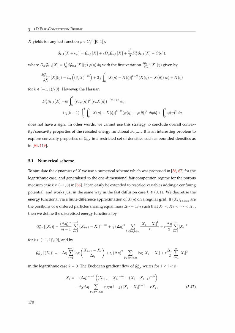
3. 1D Fair-Competition Regime
X yields for any test function ϕ P C8c pr0, 1sq,
Gk,1rX ` εϕs “ Gk,1rXs ` εDϕGk,1rXs `ε2
2 D2ϕGk,1rXs `Opε3q,
where DϕGk,1rXs “ş10 δGk,1rXspηqϕpηq dη with the first variation δGk,1
δX rXspηq given by
δGk,1δX
rXspηq “ Bη
´
pBηXq´m
¯
` 2χż 1
0|Xpηq ´Xpηq|k´2 pXpηq ´Xpηqq dη `Xpηq
for k P p´1, 1qt0u. However, the Hessian
D2ϕGk,1rXs “m
ż 1
0pBηϕpηqq
2pBηXpηqq
´pm`1qdη
`χpk ´ 1qż 1
0
ż 1
0|Xpηq ´Xpηq|
k´2pϕpηq ´ ϕpηqq
2dηdη `
ż 1
0ϕpηq2 dη
does not have a sign. In other words, we cannot use this strategy to conclude overall convex-
ity/concavity properties of the rescaled energy functional Fk,resc. It is an interesting problem to
explore convexity properties of Gk,r in a restricted set of densities such as bounded densities as
in [94, 119].
5.1 Numerical scheme
To simulate the dynamics ofX we use a numerical scheme which was proposed in [36, 67] for the
logarithmic case, and generalised to the one-dimensional fair-competition regime for the porous
medium case k P p´1, 0q in [66]. It can easily be extended to rescaled variables adding a confining
potential, and works just in the same way in the fast diffusion case k P p0, 1q. We discretise the
energy functional via a finite difference approximation ofXpηq on a regular grid. If pXiq1ďiďn are
the positions of n ordered particles sharing equal mass ∆η “ 1n such that X1 ă X2 ă ¨ ¨ ¨ ă Xn,
then we define the discretised energy functional by
Gnk,r rpXiqs “p∆ηqm
m´ 1
n´1ÿ
i“1pXi`1 ´Xiq
1´m` χ p∆ηq2
ÿ
1ďi‰jďn
|Xj ´Xi|k
k` r
∆η2
nÿ
i“1|Xi|
2
for k P p´1, 1qzt0u, and by
Gn0,r rpXiqs “ ´∆ηn´1ÿ
i“1log
ˆ
Xi`1 ´Xi
∆η
˙
` χ p∆ηq2ÿ
1ďi‰jďnlog |Xj ´Xi| ` r
∆η2
nÿ
i“1|Xi|
2
in the logarithmic case k “ 0. The Euclidean gradient flow of Gnk,r writes for 1 ă i ă n
9Xi “´ p∆ηqm´1´
pXi`1 ´Xiq´m
´ pXi ´Xi´1q´m
¯
´ 2χ∆ηÿ
1ďj‰iďnsignpi´ jq |Xi ´Xj |
k´1´ rXi , (5.47)
170
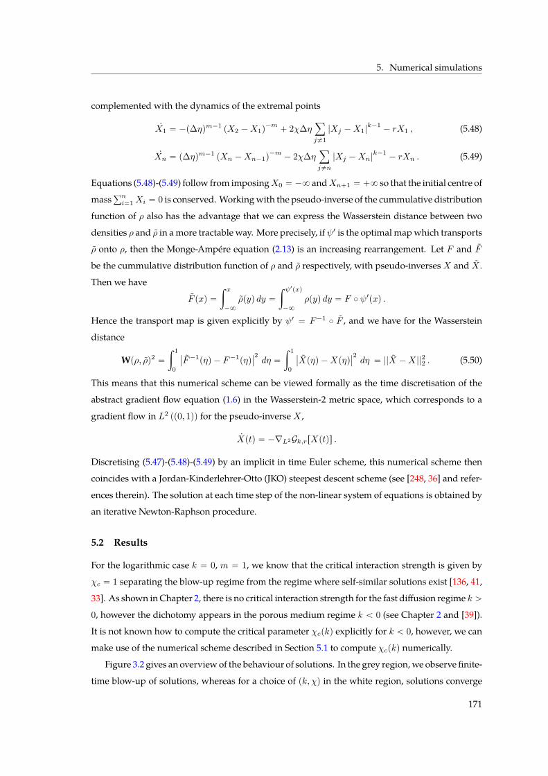
5. Numerical simulations
complemented with the dynamics of the extremal points
9X1 “ ´p∆ηqm´1 pX2 ´X1q´m
` 2χ∆ηÿ
j‰1|Xj ´X1|
k´1´ rX1 , (5.48)
9Xn “ p∆ηqm´1 pXn ´Xn´1q´m
´ 2χ∆ηÿ
j‰n
|Xj ´Xn|k´1
´ rXn . (5.49)
Equations (5.48)-(5.49) follow from imposingX0 “ ´8 andXn`1 “ `8 so that the initial centre of
massřni“1Xi “ 0 is conserved. Workingwith the pseudo-inverse of the cummulative distribution
function of ρ also has the advantage that we can express the Wasserstein distance between two
densities ρ and ρ in amore tractable way. More precisely, if ψ1 is the optimal mapwhich transports
ρ onto ρ, then the Monge-Ampére equation (2.13) is an increasing rearrangement. Let F and F
be the cummulative distribution function of ρ and ρ respectively, with pseudo-inversesX and X .
Then we have
F pxq “
ż x
´8
ρpyq dy “
ż ψ1pxq
´8
ρpyq dy “ F ˝ ψ1pxq .
Hence the transport map is given explicitly by ψ1 “ F´1 ˝ F , and we have for the Wasserstein
distance
Wpρ, ρq2 “ż 1
0
ˇ
ˇF´1pηq ´ F´1pηqˇ
ˇ
2dη “
ż 1
0
ˇ
ˇXpηq ´Xpηqˇ
ˇ
2dη “ ||X ´X||22 . (5.50)
This means that this numerical scheme can be viewed formally as the time discretisation of the
abstract gradient flow equation (1.6) in the Wasserstein-2 metric space, which corresponds to a
gradient flow in L2 pp0, 1qq for the pseudo-inverse X ,
9Xptq “ ´∇L2Gk,rrXptqs .
Discretising (5.47)-(5.48)-(5.49) by an implicit in time Euler scheme, this numerical scheme then
coincides with a Jordan-Kinderlehrer-Otto (JKO) steepest descent scheme (see [248, 36] and refer-
ences therein). The solution at each time step of the non-linear system of equations is obtained by
an iterative Newton-Raphson procedure.
5.2 Results
For the logarithmic case k “ 0, m “ 1, we know that the critical interaction strength is given by
χc “ 1 separating the blow-up regime from the regime where self-similar solutions exist [136, 41,
33]. As shown inChapter 2, there is no critical interaction strength for the fast diffusion regime k ą
0, however the dichotomy appears in the porous medium regime k ă 0 (see Chapter 2 and [39]).
It is not known how to compute the critical parameter χcpkq explicitly for k ă 0, however, we can
make use of the numerical scheme described in Section 5.1 to compute χcpkq numerically.
Figure 3.2 gives an overviewof the behaviour of solutions. In the grey region, we observe finite-
time blow-up of solutions, whereas for a choice of pk, χq in the white region, solutions converge
171
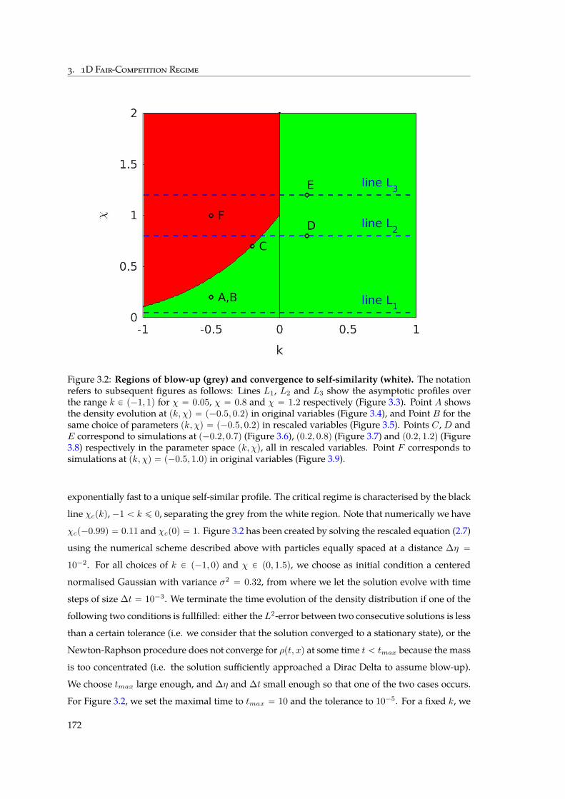
3. 1D Fair-Competition Regime
Figure 3.2: Regions of blow-up (grey) and convergence to self-similarity (white). The notationrefers to subsequent figures as follows: Lines L1, L2 and L3 show the asymptotic profiles overthe range k P p´1, 1q for χ “ 0.05, χ “ 0.8 and χ “ 1.2 respectively (Figure 3.3). Point A showsthe density evolution at pk, χq “ p´0.5, 0.2q in original variables (Figure 3.4), and Point B for thesame choice of parameters pk, χq “ p´0.5, 0.2q in rescaled variables (Figure 3.5). Points C, D andE correspond to simulations at p´0.2, 0.7q (Figure 3.6), p0.2, 0.8q (Figure 3.7) and p0.2, 1.2q (Figure3.8) respectively in the parameter space pk, χq, all in rescaled variables. Point F corresponds tosimulations at pk, χq “ p´0.5, 1.0q in original variables (Figure 3.9).
exponentially fast to a unique self-similar profile. The critical regime is characterised by the black
line χcpkq, ´1 ă k ď 0, separating the grey from the white region. Note that numerically we have
χcp´0.99q “ 0.11 and χcp0q “ 1. Figure 3.2 has been created by solving the rescaled equation (2.7)
using the numerical scheme described above with particles equally spaced at a distance ∆η “
10´2. For all choices of k P p´1, 0q and χ P p0, 1.5q, we choose as initial condition a centered
normalised Gaussian with variance σ2 “ 0.32, from where we let the solution evolve with time
steps of size ∆t “ 10´3. We terminate the time evolution of the density distribution if one of the
following two conditions is fullfilled: either the L2-error between two consecutive solutions is less
than a certain tolerance (i.e. we consider that the solution converged to a stationary state), or the
Newton-Raphson procedure does not converge for ρpt, xq at some time t ă tmax because the mass
is too concentrated (i.e. the solution sufficiently approached a Dirac Delta to assume blow-up).
We choose tmax large enough, and ∆η and ∆t small enough so that one of the two cases occurs.
For Figure 3.2, we set the maximal time to tmax “ 10 and the tolerance to 10´5. For a fixed k, we
172
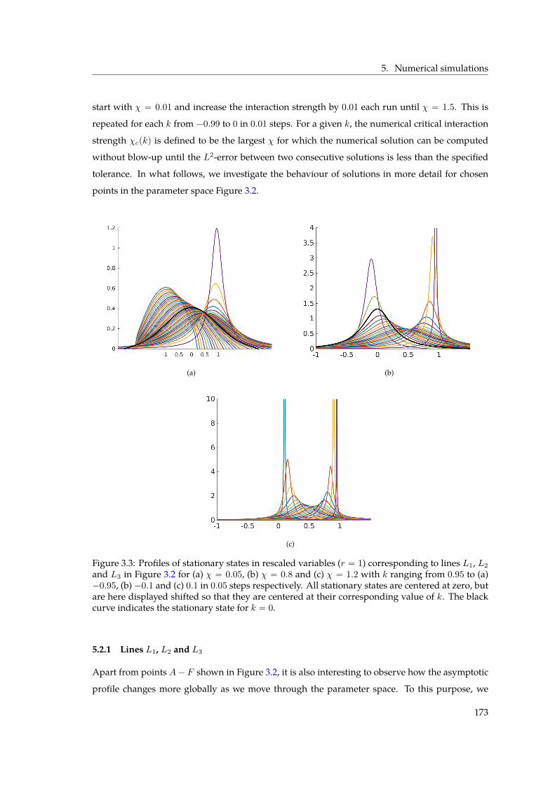
5. Numerical simulations
start with χ “ 0.01 and increase the interaction strength by 0.01 each run until χ “ 1.5. This is
repeated for each k from ´0.99 to 0 in 0.01 steps. For a given k, the numerical critical interaction
strength χcpkq is defined to be the largest χ for which the numerical solution can be computed
without blow-up until the L2-error between two consecutive solutions is less than the specified
tolerance. In what follows, we investigate the behaviour of solutions in more detail for chosen
points in the parameter space Figure 3.2.
(a) (b)
(c)
Figure 3.3: Profiles of stationary states in rescaled variables (r “ 1) corresponding to lines L1, L2and L3 in Figure 3.2 for (a) χ “ 0.05, (b) χ “ 0.8 and (c) χ “ 1.2 with k ranging from 0.95 to (a)´0.95, (b) ´0.1 and (c) 0.1 in 0.05 steps respectively. All stationary states are centered at zero, butare here displayed shifted so that they are centered at their corresponding value of k. The blackcurve indicates the stationary state for k “ 0.
5.2.1 Lines L1, L2 and L3
Apart from points A´ F shown in Figure 3.2, it is also interesting to observe how the asymptotic
profile changes more globally as we move through the parameter space. To this purpose, we
173
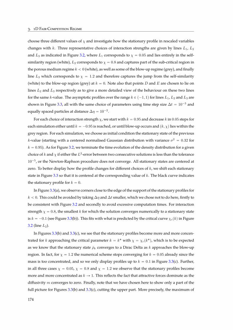
3. 1D Fair-Competition Regime
choose three different values of χ and investigate how the stationary profile in rescaled variables
changes with k. Three representative choices of interaction strengths are given by lines L1, L2
and L3 as indicated in Figure 3.2, where L1 corresponds to χ “ 0.05 and lies entirely in the self-
similarity region (white), L2 corresponds to χ “ 0.8 and captures part of the sub-critical region in
the porousmedium regime k ă 0 (white), aswell as some of the blow-up regime (grey), and finally
line L3 which corresponds to χ “ 1.2 and therefore captures the jump from the self-similarity
(white) to the blow-up region (grey) at k “ 0. Note also that points D and E are chosen to lie on
lines L2 and L3 respectively as to give a more detailed view of the behaviour on these two lines
for the same k-value. The asymptotic profiles over the range k P p´1, 1q for lines L1, L2 and L3 are
shown in Figure 3.3, all with the same choice of parameters using time step size ∆t “ 10´3 and
equally spaced particles at distance ∆η “ 10´2.
For each choice of interaction strength χ, we start with k “ 0.95 and decrease k in 0.05 steps for
each simulation either until k “ ´0.95 is reached, or until blow-up occurs and pk, χq lies within the
grey region. For each simulation, we choose as initial condition the stationary state of the previous
k-value (starting with a centered normalised Gaussian distribution with variance σ2 “ 0.32 for
k “ 0.95). As for Figure 3.2, we terminate the time evolution of the density distribution for a given
choice of k and χ if either the L2-error between two consecutive solutions is less than the tolerance
10´5, or the Newton-Raphson procedure does not converge. All stationary states are centered at
zero. To better display how the profile changes for different choices of k, we shift each stationary
state in Figure 3.3 so that it is centered at the corresponding value of k. The black curve indicates
the stationary profile for k “ 0.
In Figure 3.3(a), we observe corners close to the edge of the support of the stationary profiles for
k ă 0. This could be avoided by taking ∆η and ∆t smaller, whichwe chose not to do here, firstly to
be consistent with Figure 3.2 and secondly to avoid excessive computation times. For interaction
strength χ “ 0.8, the smallest k for which the solution converges numerically to a stationary state
is k “ ´0.1 (see Figure 3.3(b)). This fits with what is predicted by the critical curve χcpkq in Figure
3.2 (line L2).
In Figures 3.3(b) and 3.3(c), we see that the stationary profiles become more and more concen-
trated for k approaching the critical parameter k “ k˚ with χ “ χcpk˚q, which is to be expected
as we know that the stationary state ρk converges to a Dirac Delta as k approaches the blow-up
region. In fact, for χ “ 1.2 the numerical scheme stops converging for k “ 0.05 already since the
mass is too concentrated, and so we only display profiles up to k “ 0.1 in Figure 3.3(c). Further,
in all three cases χ “ 0.05, χ “ 0.8 and χ “ 1.2 we observe that the stationary profiles become
more and more concentrated as k Ñ 1. This reflects the fact that attractive forces dominate as the
diffusivitym converges to zero. Finally, note that we have chosen here to show only a part of the
full picture for Figures 3.3(b) and 3.3(c), cutting the upper part. More precisely, the maximum of
174
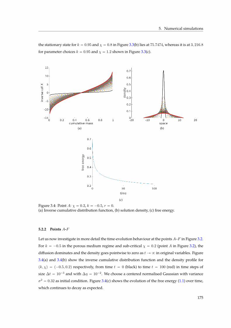
5. Numerical simulations
the stationary state for k “ 0.95 and χ “ 0.8 in Figure 3.3(b) lies at 75.7474, whereas it is at 3, 216.8
for parameter choices k “ 0.95 and χ “ 1.2 shown in Figure 3.3(c).
(a) (b)
(c)
Figure 3.4: Point A: χ “ 0.2, k “ ´0.5, r “ 0.(a) Inverse cumulative distribution function, (b) solution density, (c) free energy.
5.2.2 Points A-F
Let us now investigate inmore detail the time-evolution behaviour at the pointsA–F in Figure 3.2.
For k “ ´0.5 in the porous medium regime and sub-critical χ “ 0.2 (point A in Figure 3.2), the
diffusion dominates and the density goes pointwise to zero as tÑ8 in original variables. Figure
3.4(a) and 3.4(b) show the inverse cumulative distribution function and the density profile for
pk, χq “ p´0.5, 0.2q respectively, from time t “ 0 (black) to time t “ 100 (red) in time steps of
size ∆t “ 10´3 and with ∆η “ 10´2. We choose a centered normalised Gaussian with variance
σ2 “ 0.32 as initial condition. Figure 3.4(c) shows the evolution of the free energy (1.1) over time,
which continues to decay as expected.
175
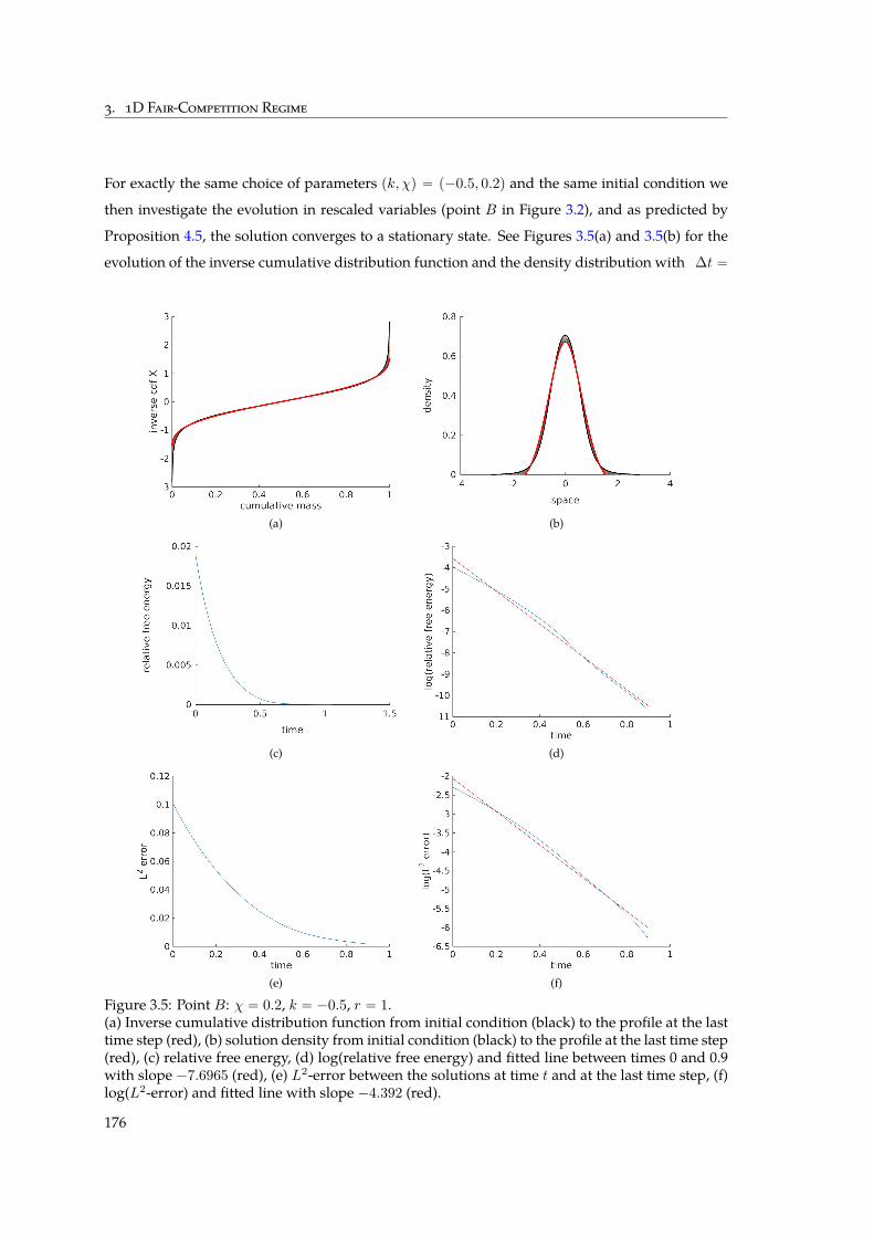
3. 1D Fair-Competition Regime
For exactly the same choice of parameters pk, χq “ p´0.5, 0.2q and the same initial condition we
then investigate the evolution in rescaled variables (point B in Figure 3.2), and as predicted by
Proposition 4.5, the solution converges to a stationary state. See Figures 3.5(a) and 3.5(b) for the
evolution of the inverse cumulative distribution function and the density distribution with ∆t “
(a) (b)
(c) (d)
(e) (f)
Figure 3.5: Point B: χ “ 0.2, k “ ´0.5, r “ 1.(a) Inverse cumulative distribution function from initial condition (black) to the profile at the lasttime step (red), (b) solution density from initial condition (black) to the profile at the last time step(red), (c) relative free energy, (d) log(relative free energy) and fitted line between times 0 and 0.9with slope ´7.6965 (red), (e) L2-error between the solutions at time t and at the last time step, (f)log(L2-error) and fitted line with slope ´4.392 (red).
176
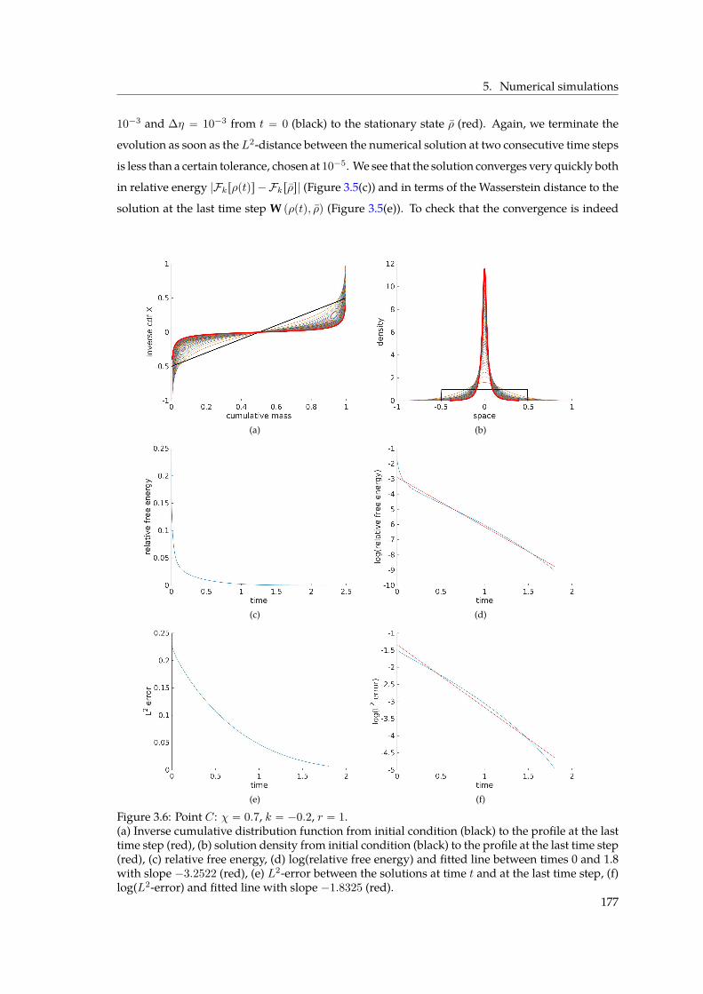
5. Numerical simulations
10´3 and ∆η “ 10´3 from t “ 0 (black) to the stationary state ρ (red). Again, we terminate the
evolution as soon as the L2-distance between the numerical solution at two consecutive time steps
is less than a certain tolerance, chosen at 10´5. We see that the solution converges very quickly both
in relative energy |Fkrρptqs ´Fkrρs| (Figure 3.5(c)) and in terms of the Wasserstein distance to the
solution at the last time step W pρptq, ρq (Figure 3.5(e)). To check that the convergence is indeed
(a) (b)
(c) (d)
(e) (f)
Figure 3.6: Point C: χ “ 0.7, k “ ´0.2, r “ 1.(a) Inverse cumulative distribution function from initial condition (black) to the profile at the lasttime step (red), (b) solution density from initial condition (black) to the profile at the last time step(red), (c) relative free energy, (d) log(relative free energy) and fitted line between times 0 and 1.8with slope ´3.2522 (red), (e) L2-error between the solutions at time t and at the last time step, (f)log(L2-error) and fitted line with slope ´1.8325 (red).
177
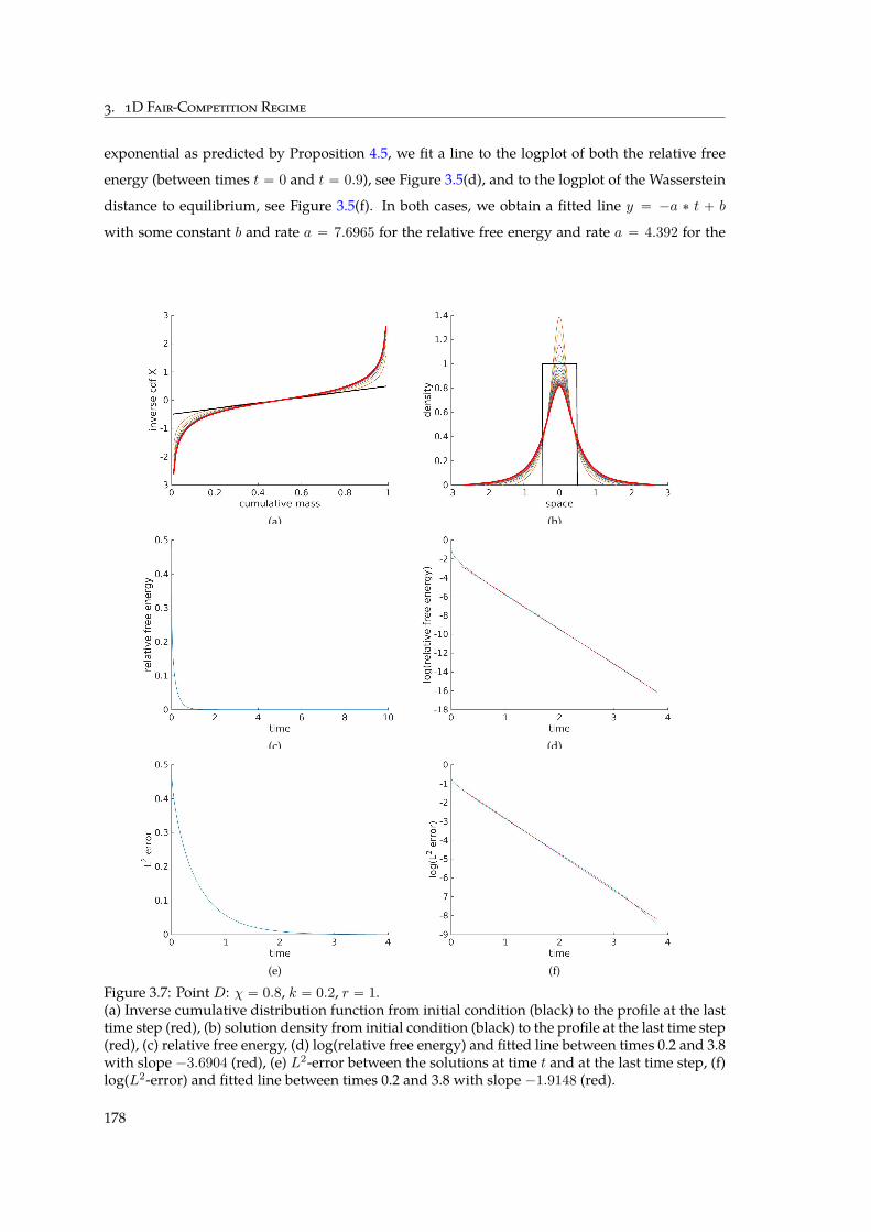
3. 1D Fair-Competition Regime
exponential as predicted by Proposition 4.5, we fit a line to the logplot of both the relative free
energy (between times t “ 0 and t “ 0.9), see Figure 3.5(d), and to the logplot of the Wasserstein
distance to equilibrium, see Figure 3.5(f). In both cases, we obtain a fitted line y “ ´a ˚ t ` b
with some constant b and rate a “ 7.6965 for the relative free energy and rate a “ 4.392 for the
(a) (b)
(c) (d)
(e) (f)
Figure 3.7: Point D: χ “ 0.8, k “ 0.2, r “ 1.(a) Inverse cumulative distribution function from initial condition (black) to the profile at the lasttime step (red), (b) solution density from initial condition (black) to the profile at the last time step(red), (c) relative free energy, (d) log(relative free energy) and fitted line between times 0.2 and 3.8with slope ´3.6904 (red), (e) L2-error between the solutions at time t and at the last time step, (f)log(L2-error) and fitted line between times 0.2 and 3.8 with slope ´1.9148 (red).
178
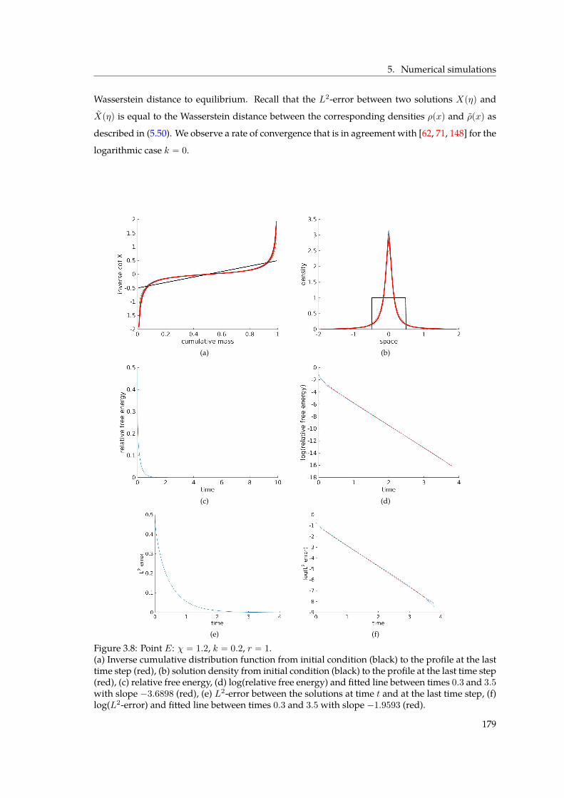
5. Numerical simulations
Wasserstein distance to equilibrium. Recall that the L2-error between two solutions Xpηq and
Xpηq is equal to the Wasserstein distance between the corresponding densities ρpxq and ρpxq as
described in (5.50). We observe a rate of convergence that is in agreement with [62, 71, 148] for the
logarithmic case k “ 0.
(a) (b)
(c) (d)
(e) (f)
Figure 3.8: Point E: χ “ 1.2, k “ 0.2, r “ 1.(a) Inverse cumulative distribution function from initial condition (black) to the profile at the lasttime step (red), (b) solution density from initial condition (black) to the profile at the last time step(red), (c) relative free energy, (d) log(relative free energy) and fitted line between times 0.3 and 3.5with slope ´3.6898 (red), (e) L2-error between the solutions at time t and at the last time step, (f)log(L2-error) and fitted line between times 0.3 and 3.5 with slope ´1.9593 (red).
179
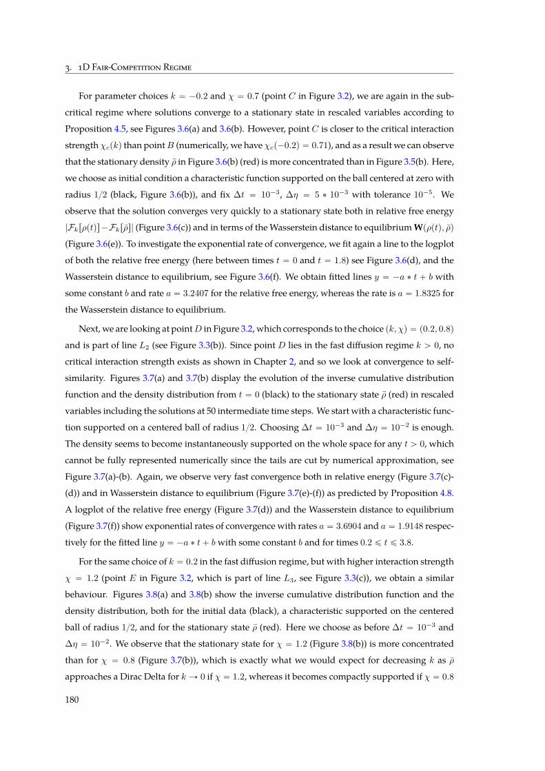
3. 1D Fair-Competition Regime
For parameter choices k “ ´0.2 and χ “ 0.7 (point C in Figure 3.2), we are again in the sub-
critical regime where solutions converge to a stationary state in rescaled variables according to
Proposition 4.5, see Figures 3.6(a) and 3.6(b). However, point C is closer to the critical interaction
strength χcpkq than pointB (numerically, we have χcp´0.2q “ 0.71), and as a result we can observe
that the stationary density ρ in Figure 3.6(b) (red) is more concentrated than in Figure 3.5(b). Here,
we choose as initial condition a characteristic function supported on the ball centered at zero with
radius 12 (black, Figure 3.6(b)), and fix ∆t “ 10´3, ∆η “ 5 ˚ 10´3 with tolerance 10´5. We
observe that the solution converges very quickly to a stationary state both in relative free energy
|Fkrρptqs´Fkrρs| (Figure 3.6(c)) and in terms of theWasserstein distance to equilibriumWpρptq, ρq
(Figure 3.6(e)). To investigate the exponential rate of convergence, we fit again a line to the logplot
of both the relative free energy (here between times t “ 0 and t “ 1.8) see Figure 3.6(d), and the
Wasserstein distance to equilibrium, see Figure 3.6(f). We obtain fitted lines y “ ´a ˚ t ` b with
some constant b and rate a “ 3.2407 for the relative free energy, whereas the rate is a “ 1.8325 for
the Wasserstein distance to equilibrium.
Next, we are looking at pointD in Figure 3.2, which corresponds to the choice pk, χq “ p0.2, 0.8q
and is part of line L2 (see Figure 3.3(b)). Since point D lies in the fast diffusion regime k ą 0, no
critical interaction strength exists as shown in Chapter 2, and so we look at convergence to self-
similarity. Figures 3.7(a) and 3.7(b) display the evolution of the inverse cumulative distribution
function and the density distribution from t “ 0 (black) to the stationary state ρ (red) in rescaled
variables including the solutions at 50 intermediate time steps. We start with a characteristic func-
tion supported on a centered ball of radius 12. Choosing ∆t “ 10´3 and ∆η “ 10´2 is enough.
The density seems to become instantaneously supported on the whole space for any t ą 0, which
cannot be fully represented numerically since the tails are cut by numerical approximation, see
Figure 3.7(a)-(b). Again, we observe very fast convergence both in relative energy (Figure 3.7(c)-
(d)) and in Wasserstein distance to equilibrium (Figure 3.7(e)-(f)) as predicted by Proposition 4.8.
A logplot of the relative free energy (Figure 3.7(d)) and the Wasserstein distance to equilibrium
(Figure 3.7(f)) show exponential rates of convergence with rates a “ 3.6904 and a “ 1.9148 respec-
tively for the fitted line y “ ´a ˚ t` bwith some constant b and for times 0.2 ď t ď 3.8.
For the same choice of k “ 0.2 in the fast diffusion regime, but with higher interaction strength
χ “ 1.2 (point E in Figure 3.2, which is part of line L3, see Figure 3.3(c)), we obtain a similar
behaviour. Figures 3.8(a) and 3.8(b) show the inverse cumulative distribution function and the
density distribution, both for the initial data (black), a characteristic supported on the centered
ball of radius 12, and for the stationary state ρ (red). Here we choose as before ∆t “ 10´3 and
∆η “ 10´2. We observe that the stationary state for χ “ 1.2 (Figure 3.8(b)) is more concentrated
than for χ “ 0.8 (Figure 3.7(b)), which is exactly what we would expect for decreasing k as ρ
approaches a Dirac Delta for k Ñ 0 if χ “ 1.2, whereas it becomes compactly supported if χ “ 0.8
180
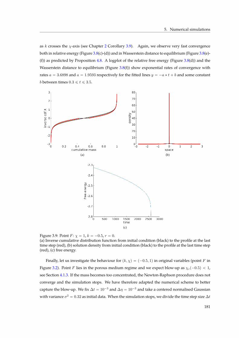
5. Numerical simulations
as k crosses the χ-axis (see Chapter 2 Corollary 3.9). Again, we observe very fast convergence
both in relative energy (Figure 3.8(c)-(d)) and inWasserstein distance to equilibrium (Figure 3.8(e)-
(f)) as predicted by Proposition 4.8. A logplot of the relative free energy (Figure 3.8(d)) and the
Wasserstein distance to equilibrium (Figure 3.8(f)) show exponential rates of convergence with
rates a “ 3.6898 and a “ 1.9593 respectively for the fitted lines y “ ´a ˚ t` b and some constant
b between times 0.3 ď t ď 3.5.
(a) (b)
(c)
Figure 3.9: Point F : χ “ 1, k “ ´0.5, r “ 0.(a) Inverse cumulative distribution function from initial condition (black) to the profile at the lasttime step (red), (b) solution density from initial condition (black) to the profile at the last time step(red), (c) free energy.
Finally, let us investigate the behaviour for pk, χq “ p´0.5, 1q in original variables (point F in
Figure 3.2). Point F lies in the porous medium regime and we expect blow-up as χcp´0.5q ă 1,
see Section 4.1.3. If the mass becomes too concentrated, the Newton-Raphson procedure does not
converge and the simulation stops. We have therefore adapted the numerical scheme to better
capture the blow-up. We fix ∆t “ 10´3 and ∆η “ 10´3 and take a centered normalised Gaussian
with variance σ2 “ 0.32 as initial data. When the simulation stops, we divide the time step size ∆t
181
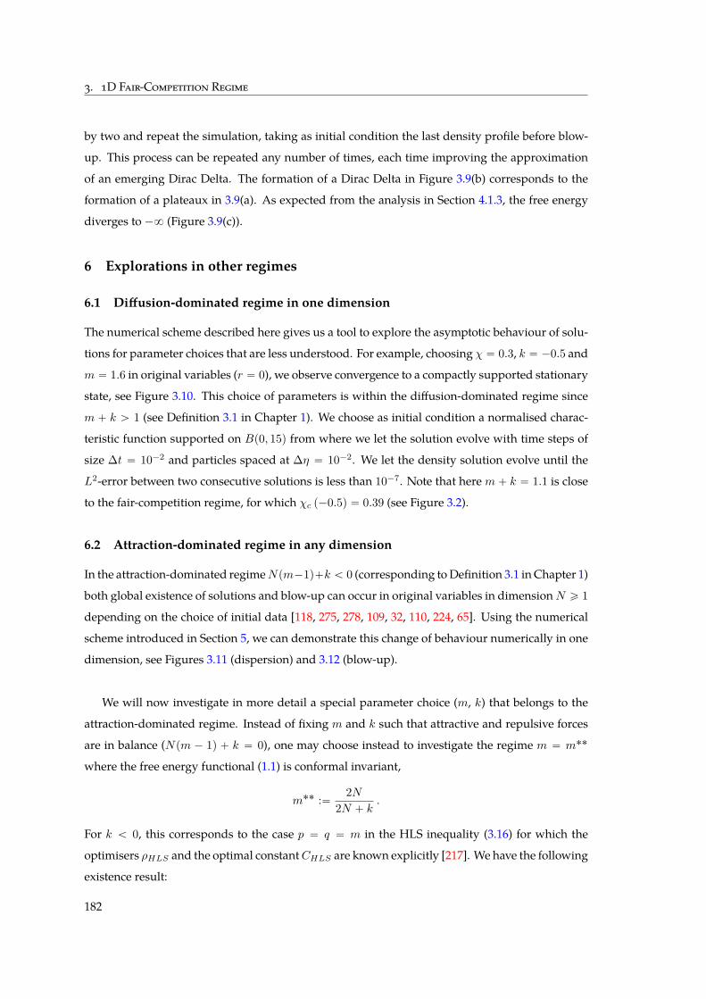
3. 1D Fair-Competition Regime
by two and repeat the simulation, taking as initial condition the last density profile before blow-
up. This process can be repeated any number of times, each time improving the approximation
of an emerging Dirac Delta. The formation of a Dirac Delta in Figure 3.9(b) corresponds to the
formation of a plateaux in 3.9(a). As expected from the analysis in Section 4.1.3, the free energy
diverges to ´8 (Figure 3.9(c)).
6 Explorations in other regimes
6.1 Diffusion-dominated regime in one dimension
The numerical scheme described here gives us a tool to explore the asymptotic behaviour of solu-
tions for parameter choices that are less understood. For example, choosing χ “ 0.3, k “ ´0.5 and
m “ 1.6 in original variables (r “ 0), we observe convergence to a compactly supported stationary
state, see Figure 3.10. This choice of parameters is within the diffusion-dominated regime since
m ` k ą 1 (see Definition 3.1 in Chapter 1). We choose as initial condition a normalised charac-
teristic function supported on Bp0, 15q from where we let the solution evolve with time steps of
size ∆t “ 10´2 and particles spaced at ∆η “ 10´2. We let the density solution evolve until the
L2-error between two consecutive solutions is less than 10´7. Note that herem` k “ 1.1 is close
to the fair-competition regime, for which χc p´0.5q “ 0.39 (see Figure 3.2).
6.2 Attraction-dominated regime in any dimension
In the attraction-dominated regimeNpm´1q`k ă 0 (corresponding toDefinition 3.1 in Chapter 1)
both global existence of solutions and blow-up can occur in original variables in dimensionN ě 1
depending on the choice of initial data [118, 275, 278, 109, 32, 110, 224, 65]. Using the numerical
scheme introduced in Section 5, we can demonstrate this change of behaviour numerically in one
dimension, see Figures 3.11 (dispersion) and 3.12 (blow-up).
We will now investigate in more detail a special parameter choice (m, k) that belongs to the
attraction-dominated regime. Instead of fixing m and k such that attractive and repulsive forces
are in balance (Npm ´ 1q ` k “ 0), one may choose instead to investigate the regime m “ m˚˚
where the free energy functional (1.1) is conformal invariant,
m˚˚ :“ 2N2N ` k .
For k ă 0, this corresponds to the case p “ q “ m in the HLS inequality (3.16) for which the
optimisers ρHLS and the optimal constantCHLS are known explicitly [217]. We have the following
existence result:
182
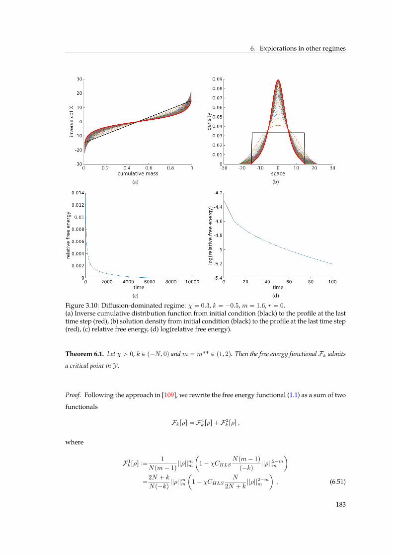
6. Explorations in other regimes
(a) (b)
(c) (d)
Figure 3.10: Diffusion-dominated regime: χ “ 0.3, k “ ´0.5,m “ 1.6, r “ 0.(a) Inverse cumulative distribution function from initial condition (black) to the profile at the lasttime step (red), (b) solution density from initial condition (black) to the profile at the last time step(red), (c) relative free energy, (d) log(relative free energy).
Theorem 6.1. Let χ ą 0, k P p´N, 0q andm “ m˚˚ P p1, 2q. Then the free energy functional Fk admits
a critical point in Y .
Proof. Following the approach in [109], we rewrite the free energy functional (1.1) as a sum of two
functionals
Fkrρs “ F1k rρs ` F2
k rρs ,
where
F1k rρs :“ 1
Npm´ 1q ||ρ||mm
ˆ
1´ χCHLSNpm´ 1qp´kq
||ρ||2´mm
˙
“2N ` kNp´kq
||ρ||mm
ˆ
1´ χCHLSN
2N ` k ||ρ||2´mm
˙
, (6.51)
183
3. 1D Fair-Competition Regime
and
F2k rρs :“ χ
p´kq
¨
˝CHLS ||ρ||2m ´
ij
RNˆRN
|x´ y|kρpxqρpyq dxdy
˛
‚ . (6.52)
By the HLS inequality (3.16), the second functional (6.52) is bounded below for any χ ą 0,
F2k rρs ě 0 , @ρ P Y ,
and by [217, Theorem 3.1], there exists a family of optimisers ρHLS,λ,c,
ρHLS,λ,cpxq “ c
ˆ
λ
λ2 ` |x|2
˙Nm
, λ ą 0, c ą 0 (6.53)
satisfying F2k rρHLS,λ,cs “ 0 with the optimal constant CHLS given by
CHLS :“ π´k2
˜
Γ`
N`k2
˘
Γ`
N ` k2˘
¸˜
Γ`
N2˘
Γ pNq
¸´pN`kqN
.
The parameter λ ą 0 in (6.53) corresponds to the scaling that leaves the Lm-norm of ρHLS,λ,cinvariant. Since the first variation of the functional F1
k defined in (6.51) is given by
δF1k
δρrρspxq “
2p´kq
`
1´ χCHLS ||ρ||2´mm
˘
ρm´1pxq
and since the Lm-norm of the optimiser can be calculated explicitly,
||ρHLS,λ,c||m “ c
˜
21´NπN`1
2
Γ`
N`12
˘
¸1m
,
there exists a unique choice of pλ, cq “ pλ˚, c˚q for each χ ą 0 such that
δF1k
δρrρHLS,λ˚,c˚spxq “ 0 and
ż
RNρHLS,λ˚,c˚pxq dx “ 1
given by
c˚pχq :“˜
21´NπN`1
2
Γ`
N`12
˘
¸´1m
pχCHLSq1pm´2q
, λ˚pχq :“ˆż
RNρHLS,1,c˚pχqpxq dx
˙2k. (6.54)
Hence ρHLS,λ˚,c˚ is a critical point of Fk in Y .
We can choose to leave λ ą 0 as a free parameter in (6.53), only fixing c “ c˚pχq so that
ρHLS,λ,c˚ is a critical point of Fk with arbitrary mass. We conjecture that a similar result to [109,
Theorem 2.1] holds true for general k P p´N, 0q andm “ m˚˚ for radially symmetric initial data:
184
6. Explorations in other regimes
Conjecture 1 (Global Existence vs Blow-up). Let χ ą 0, k P p´N, 0q and m “ m˚˚ in dimension
N ě 1. Assume the initial datum ρ0 P Y is radially symmetric.
(i) If there exists λ0 ą 0 such that
ρ0prq ă ρHLS,λ0,c˚prq , @ r ě 0, ,
then any radially symmetric solution ρpt, rq of (1.4) with initial datum ρp0, rq “ ρ0prq is vanishing
in L1loc
`
RN˘
as tÑ8.
(ii) If there exists λ0 ą 0 such that
ρ0prq ą ρHLS,λ0,c˚prq , @ r ě 0 ,
then any radially symmetric solution ρpt, rq of (1.4)with initial datum ρp0, rq “ ρ0prqmust blow-up
at a finite time T˚ or has a mass concentration at r “ 0 as time goes to infinity in the sense that there
exist Rptq Ñ 0 as tÑ8 and a positive constant C ą 0 such thatż
Bp0,Rptqqρpt, xq dx ě C .
Further, we expect the following to be true analogous to [109]:
Conjecture 2 (Unstable Stationary State). For any χ ą 0, the density ρHLS,λ˚,c˚ P Y with pλ˚, c˚q
given by (6.54) is an unstable stationary state of equation (1.4).
Numerically, we indeed observe the behaviour predicted in Conjecture 1 for N “ 1. Using
the scheme introduced in Section 5, we choose as initial data the density ρHLS,λ0,c0 given by the
optimisers of the HLS inequality (6.53). For any choice of c0 ą 0, we fix λ0 ą 0 such that ρHLS,λ0,c0
has unit mass and is therefore in Y . Note that ρHLS,λ0,c0 is not a critical point of Fk unless c0 “ c˚.
Comparing with the stationary state ρHLS,λ0,c˚ , we have
sign pc˚ ´ c0q “ sign`
ρHLS,λ0,c˚pxq ´ ρHLS,λ0,c0pxq˘
, @x P R .
Note that the mass of the stationary state ρHLS,λ0,c˚ is given byż
RNρHLS,λ0,c˚pχqpxq dx “ λ
´k20
ż
RNρHLS,1,c˚pχqpxq dx ,
which is equal to one if and only if λ0 “ λ˚, that is c0 “ c˚. If we choose c0 ă c˚, then
ρ0 :“ ρHLS,λ0,c0 ă ρHLS,λ0,c˚ and according to Conjecture 1(i), we would expect the solution
ρpt, rq to vanish in L1loc pRq. This is exactly what can be observed in Figure 3.11 for the choice of
parameters χ “ 0.35, k “ ´12, m “ 43 in original variables (r “ 0) and with c0 “ 0.4 c˚. Here,
185
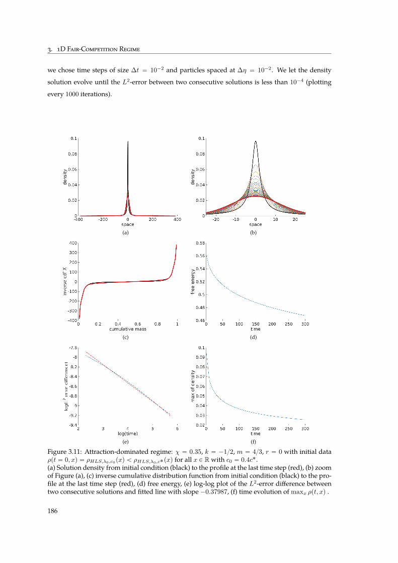
3. 1D Fair-Competition Regime
we chose time steps of size ∆t “ 10´2 and particles spaced at ∆η “ 10´2. We let the density
solution evolve until the L2-error between two consecutive solutions is less than 10´4 (plotting
every 1000 iterations).
(a) (b)
(c) (d)
(e) (f)
Figure 3.11: Attraction-dominated regime: χ “ 0.35, k “ ´12, m “ 43, r “ 0 with initial dataρpt “ 0, xq “ ρHLS,λ0,c0pxq ă ρHLS,λ0,c˚pxq for all x P Rwith c0 “ 0.4c˚.(a) Solution density from initial condition (black) to the profile at the last time step (red), (b) zoomof Figure (a), (c) inverse cumulative distribution function from initial condition (black) to the pro-file at the last time step (red), (d) free energy, (e) log-log plot of the L2-error difference betweentwo consecutive solutions and fitted line with slope ´0.37987, (f) time evolution of maxx ρpt, xq .
186
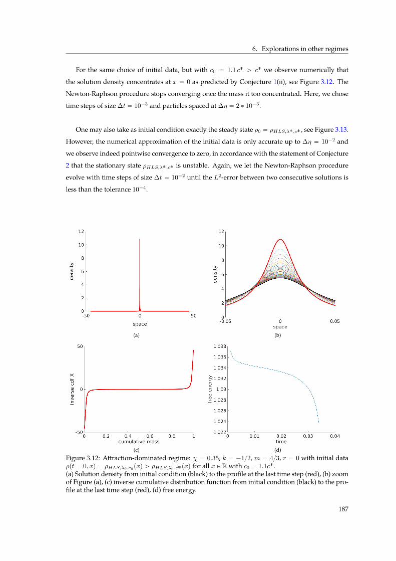
6. Explorations in other regimes
For the same choice of initial data, but with c0 “ 1.1 c˚ ą c˚ we observe numerically that
the solution density concentrates at x “ 0 as predicted by Conjecture 1(ii), see Figure 3.12. The
Newton-Raphson procedure stops converging once the mass it too concentrated. Here, we chose
time steps of size ∆t “ 10´3 and particles spaced at ∆η “ 2 ˚ 10´3.
One may also take as initial condition exactly the steady state ρ0 “ ρHLS,λ˚,c˚ , see Figure 3.13.
However, the numerical approximation of the initial data is only accurate up to ∆η “ 10´2 and
we observe indeed pointwise convergence to zero, in accordance with the statement of Conjecture
2 that the stationary state ρHLS,λ˚,c˚ is unstable. Again, we let the Newton-Raphson procedure
evolve with time steps of size ∆t “ 10´2 until the L2-error between two consecutive solutions is
less than the tolerance 10´4.
(a) (b)
(c) (d)Figure 3.12: Attraction-dominated regime: χ “ 0.35, k “ ´12, m “ 43, r “ 0 with initial dataρpt “ 0, xq “ ρHLS,λ0,c0pxq ą ρHLS,λ0,c˚pxq for all x P R with c0 “ 1.1c˚.(a) Solution density from initial condition (black) to the profile at the last time step (red), (b) zoomof Figure (a), (c) inverse cumulative distribution function from initial condition (black) to the pro-file at the last time step (red), (d) free energy.
187
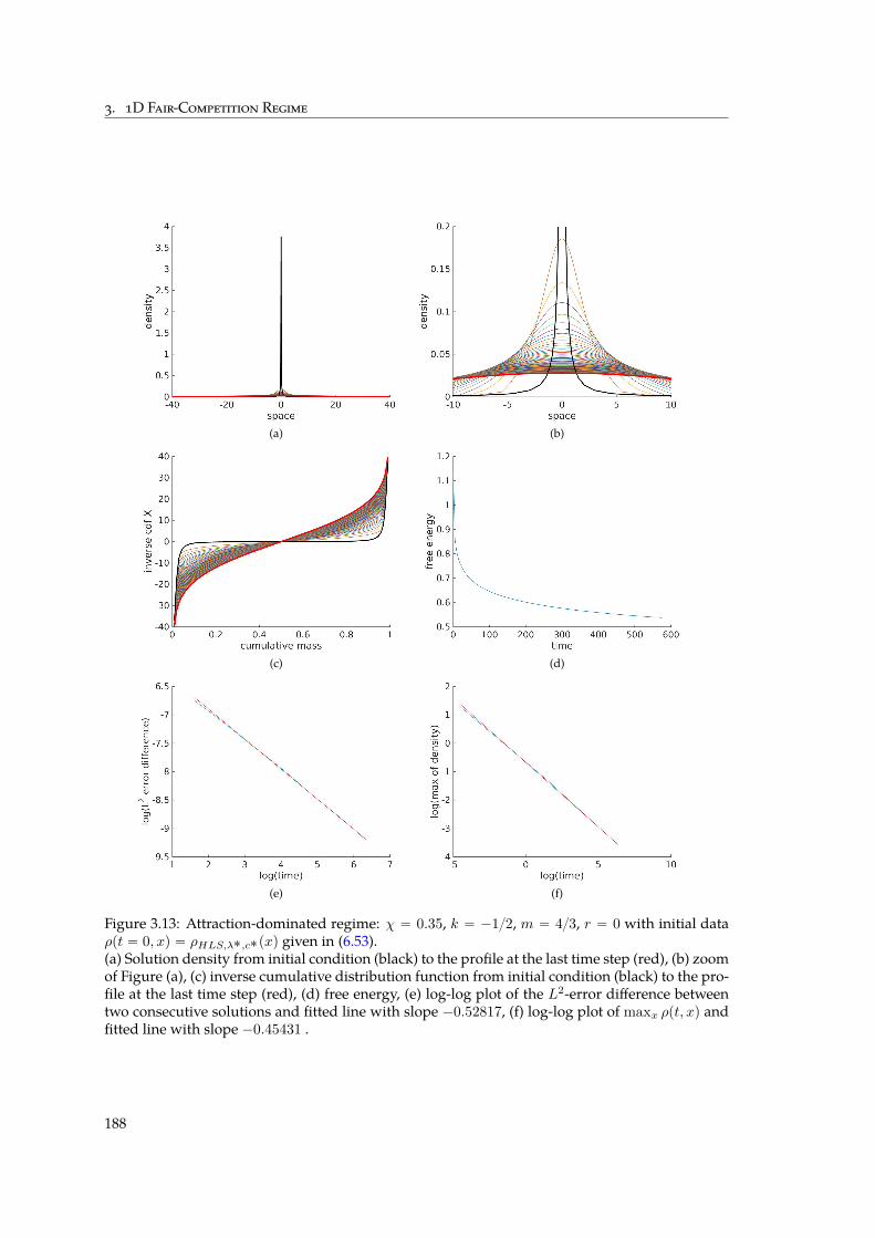
3. 1D Fair-Competition Regime
(a) (b)
(c) (d)
(e) (f)
Figure 3.13: Attraction-dominated regime: χ “ 0.35, k “ ´12, m “ 43, r “ 0 with initial dataρpt “ 0, xq “ ρHLS,λ˚,c˚pxq given in (6.53).(a) Solution density from initial condition (black) to the profile at the last time step (red), (b) zoomof Figure (a), (c) inverse cumulative distribution function from initial condition (black) to the pro-file at the last time step (red), (d) free energy, (e) log-log plot of the L2-error difference betweentwo consecutive solutions and fitted line with slope ´0.52817, (f) log-log plot of maxx ρpt, xq andfitted line with slope ´0.45431 .
188
Chapter4
Ground States in the
Diffusion-Dominated Regime
This chapter follows in most parts the article “Ground states in the diffusion-dominated regime”
written in collaboration with José A. Carrillo1, Edoardo Mainini2 and Bruno Volzone3, and sub-
mitted for publication. The radiality proof in Section 2.1 of Chapter 4 was contributed by José A.
Carrillo and Bruno Volzone.
Chapter Summary
We consider macroscopic descriptions of particles where repulsion is modelled by non-
linear power-law diffusion and attraction by a homogeneous singular kernel leading to vari-
ants of the Keller–Segel model of chemotaxis. We analyse the regime in which diffusive forces
are stronger than attraction between particles, known as the diffusion-dominated regime, and
show that all stationary states of the system are radially symmetric decreasing and compactly
supported. The model can be formulated as a gradient flow of a free energy functional for
which the overall convexity properties are not known. We show that global minimisers of the
free energy always exist. Further, they are radially symmetric, compactly supported, uniformly
bounded and C8 inside their support. Global minimisers enjoy certain regularity properties if
the diffusion is not too slow, and in this case, provide stationary states of the system. In one
dimension, stationary states are characterised as optimisers of a functional inequality which es-
tablishes equivalence between global minimisers and stationary states, and allows to deduce
uniqueness.
1Department of Mathematics, Imperial College London, South Kensington Campus, London SW7 2AZ, UK.2Dipartimento di Ingegneria Meccanica, Università degli Studi di Genova, Genova, Italia3Dipartimento di Ingegneria, Università degli Studi di Napoli “Parthenope”, Napoli, Italia
189
4. Diffusion-Dominated Regime
Chapter Content
1 Introduction . . . . . . . . . . . . . . . . . . . . . . . . . . . . . . . . . . . . . . . 191
2 Stationary states . . . . . . . . . . . . . . . . . . . . . . . . . . . . . . . . . . . . 193
2.1 Radial symmetry of stationary states . . . . . . . . . . . . . . . . . . . . 194
2.2 Stationary states are compactly supported . . . . . . . . . . . . . . . . . 196
3 Global minimisers . . . . . . . . . . . . . . . . . . . . . . . . . . . . . . . . . . . 198
3.1 Existence of global minimisers . . . . . . . . . . . . . . . . . . . . . . . . 198
3.2 Boundedness of global minimisers . . . . . . . . . . . . . . . . . . . . . 200
3.3 Regularity properties of global minimisers . . . . . . . . . . . . . . . . . 205
4 Uniqueness in one dimension . . . . . . . . . . . . . . . . . . . . . . . . . . . . . 210
4.1 Optimal transport tools . . . . . . . . . . . . . . . . . . . . . . . . . . . . 210
4.2 Functional inequality in one dimension . . . . . . . . . . . . . . . . . . . 211
A Appendix: Properties of the Riesz potential . . . . . . . . . . . . . . . . . . . . . 213
Man begreift nur,
was man selbst machen kann,
und man faßt nur,
was man selbst hervorbringen kann4.
Johann Wolfgang von Goethe
4quoted from a letter from Johann Wolfgang von Goethe to Carl Friedrich Zelter, 28th March 1804 [299].
190
1. Introduction
1 Introduction
As in Chapters 2 and 3, we are interested in the aggregation-diffusion equation
Btρ “1N
∆ρm ` 2χ∇ ¨ pρ∇Skq (1.1)
for a density ρpt, xq of unitmass defined onR`ˆRN , andwherewedenote themean-field potential
by Skpxq :“Wkpxq ˚ ρpxqwith the interaction kernelWk given by the Riesz potential,
Wkpxq :“ |x|k
k, k P p´N, 0q.
For an extensive survey of applications and literature around equation (1.1), see Chapters 1, 2 and
3. In this chapter, we focus on the case when diffusion is non-linear and of porous medium type
m ą 1 whilst Wk has a singularity at the origin k ă 0. The lower bound on k ensures that the
kernelWk is locally integrable inRN . As the Riesz potentialWk is the fundamental solution of the
fractional Laplacian p´∆qs with k “ 2s´N , we sometimes use the notation s P p0, N2q instead of
k P p´N, 0q. More precisely, the convolution term Sk is governed by a fractional diffusion process,
cN,sp´∆qsSk “ ρ , cN,s :“ p2s´NqΓ`
N2 ´ s
˘
πN24sΓpsq.
For k ą 1 ´ N , the gradient ∇Sk :“ ∇ pWk ˚ ρq is well defined locally. For k P p´N, 1´N s
however, it becomes a singular integral, and we thus define it via a Cauchy principal value,
∇Skpxq :“
$
’
’
&
’
’
%
∇ pWk ˚ ρq pxq , if 1´N ă k ă 0 ,ż
RN∇Wkpx´ yq pρpyq ´ ρpxqq dy , if ´N ă k ď 1´N .
(1.2)
The parameter χ ą 0 denotes the interaction strength and scales with the mass of solutions. Since
(1.1) conserves mass, is positivity preserving and invariant by translation, we work with solutions
ρ in the set
Y :“"
ρ P L1`pRN q X LmpRN q , ||ρ||1 “ 1 ,
ż
RNxρpxq dx “ 0
*
.
The associated free energy functional to the evolution equation (1.1) is given by
Fm,krρs :“ Hmrρs ` χWkrρs
with
Hmrρs :“ 1Npm´ 1q
ż
RNρmpxq dx , Wkrρs :“
ij
RNˆRN
|x´ y|k
kρpxqρpyq dxdy
Note thatFm,k ă 8 onY . The noticeable characteristic of the class of PDEs (1.1) and the functional
Fm,k consists in the competition between non-linear diffusion and a non-local quadratic interac-
tion term which is due to the self-attraction of the particles through the mean-field potential Sk.
The free energy functional Fm,k is not only non-increasing along the trajectories of the system,
191
4. Diffusion-Dominated Regime
equation (1.1) is also the formal gradient flow of Fm,k when the space of probability measures is
endowed with the Euclidean Wasserstein metric W, see Chapter 1 Section 2.3.2. This means that
the family of PDEs (1.1) can be written as
Btρptq “ ´∇WFm,krρptqs .
Performing gradient flows of a convex functional is a natural task, and suitable estimates from
below on the right notion of Hessian of Fm,k translate into a rate of convergence towards equilib-
rium for the PDE [295, 96, 3]. However, in our case, the overall convexity properties of the free
energy functional Fm,k are not known, see Chapter 1 Section 2.3. Performing gradient flows of
functionals with convex and concave contributions is much more delicate, and one has to seek
compensations. Such compensations do exist in our case, and we will observe them at the level of
existence of minimisers for the free energy functional Fm,k and stationary states of the family of
PDEs (1.1) for certain ranges of the diffusion exponentm ą 1.
The functionalFm,k possesses remarkable homogeneity properties thatmotivate the definition
of the fair-competition regimeNpm´1q`k “ 0, the diffusion-dominated regimeNpm´1q`k ą 0 and
the attraction-dominated regime Npm´ 1q ` k ă 0, see Chapter 1 Definition 3.1. An overview of the
parameter space pk,mq and the different regimes is given in Chapter 1 Figure 1.4. More precisely,
taking mass-preserving dilations ρλpxq :“ λNρpλxq for λ ą 0 of a density ρ P Y , we obtain
Fm,krρλs “ λNpm´1qHmrρs ` λ´kχWkrρs .
In other words, the diffusion and aggregation forces are in balance if Npm´ 1q “ ´k. This is the
case for choosing the critical diffusion exponent
mc :“ 1´ k
N. (1.3)
In this chapter, we deal with the diffusion-dominated regime m ą mc, i.e. diffusion is expected
to overcome aggregation as λ Ñ 8, for any choice of χ ą 0. This domination effect means that
solutions exist globally in time and are bounded uniformly in time [61, 277, 276]. Stationary states
were found byminimisation of the free energy functional in two and three dimensions [273, 78, 99]
in the case of attractive Newtonian potentials k “ 2´N . Stationary states are radially symmetric
if 2´N ď k ă 0 as proven in [89]. Moreover, in the particular case of N “ 2, k “ 0, andm ą 1 it
has been shown in [89] that the asymptotic behaviour is given by compactly supported stationary
solutions independently of χ. For a detailed review of known results, see Chapter 1 Section 3.
Our goal is to generalise these results to the full range k P p´N, 0q andm ą mc. Stationary states
of the system (1.1) provide natural candidates for asymptotic profiles of the evolution problem,
and we focus therefore on understanding the stationary problem first, making the connection to
192
2. Stationary states
minimisers of the energy functional Fm,k. In what follows, we denote F :“ Fm,k for simplicity.
Further, we define the diffusion exponent m˚ that will play an important role for the regularity
properties of global minimisers of F :
m˚ :“
$
’
&
’
%
2´k´N1´k´N , if N ě 1 and ´N ă k ă 1´N ,
`8 if N ě 2 and 1´N ď k ă 0 .(1.4)
In this chapter, we will prove the following main results:
Theorem 1.1. Let N ě 1, χ ą 0 and k P p´N, 0q. All stationary states of equation (1.1) are radially
symmetric decreasing. If m ą mc, then there exists a global minimiser ρ of F on Y . Further, all global
minimisers ρ P Y are radially symmetric non-increasing, compactly supported, uniformly bounded and
C8 inside their support. Moreover, all global minimisers of F are stationary states of (1.1) whenever
mc ă m ă m˚. Finally, ifmc ă m ď 2, we have ρ P W1,8 `
RN˘
.
Theorem 1.2. Let N “ 1, χ ą 0 and k P p´1, 0q. All stationary states of (1.1) are global minimisers of
the energy functional F on Y . Further, stationary states of (1.1) in Y are unique.
2 Stationary states
Let us begin by defining precisely the notion of stationary states to the aggregation-diffusion equa-
tion (1.1).
Definition 2.1. Given ρ P L1`
`
RN˘
X L8`
RN˘
with ||ρ||1 “ 1, and letting Sk “ Wk ˚ ρ, we say that
ρ is a stationary state for the evolution equation (1.1) if ρm P W1,2loc
`
RN˘
, ∇Sk P L1loc
`
RN˘
, and it
satisfies1N
∇ρm “ ´2χ ρ∇Sk
in the sense of distributions in RN . If ´N ă k ď 1 ´ N , we further require ρ P C0,α `RN˘
for some
α P p1´ k ´N, 1q.
In fact, as shown in Chapter 2, the function Sk and its gradient defined in (1.2) satisfy even
more than the regularity ∇Sk P L1loc
`
RN˘
required in Definition 2.1:
Lemma 2.2. Let ρ P L1`
`
RN˘
XL8`
RN˘
with ||ρ||1 “ 1 and k P p´N, 0q. Then the following regularity
properties hold:
(i) Sk P L8`
RN˘
.
(ii) ∇Sk P L8`
RN˘
, assuming additionally ρ P C0,α `RN˘
with α P p1 ´ k ´ N, 1q in the range
k P p´N, 1´N s.
193
4. Diffusion-Dominated Regime
Using the same techniques as in Chapter 2, we can show that Lemma 2.2 implies further reg-
ularity properties for stationary states of (1.1).
Proposition 2.3. Let k P p´N, 0q andm ą mc. If ρ is a stationary state of equation (1.1) and Sk “Wk˚ρ,
then ρ is continuous on RN , ρm´1 P W1,8 `
RN˘
, and it satisfies
ρpxqm´1 “Npm´ 1q
m
`
Crρspxq ´ 2χSkpxq˘
`, @x P RN ,
where Crρspxq is constant on each connected component of supp pρq.
It follows fromProposition 2.3 that any stationary state ρ of equation (1.1) enjoysW1,8-regularity
in the casemc ă m ď 2.
2.1 Radial symmetry of stationary states
The aim of this section is to prove that stationary states of (1.1) are radially symmetric. This is one
of the main results of [89], and is achieved there under the assumption that the interaction kernel
is not more singular than the Newtonian potential close to the origin. As we will briefly describe
in the proof of the next result, the main arguments continue to hold even for the more singular
Riesz kernelsWk.
Theorem 2.4 (Radiality of stationary states). Let χ ą 0 and m ą mc. If ρ P L1`pRN q X L8pRN q
with ρ1 “ 1 is a stationary state of (1.1) in the sense of Definition 2.1, then ρ is radially symmetric
non-increasing up to a translation.
Proof. The proof is based on a contradiction argument, being an adaptation of that in [89, Theo-
rem 2.2], to which we address the reader the more technical details. Assume that ρ is not radially
decreasing up to any translation. By Proposition 2.3, we have
ˇ
ˇ∇ρm´1pxqˇ
ˇ ď c (2.5)
for some positive constant c in supppρq. Let us now introduce the continuous Steiner symmetrisation
Sτ ρ in direction e1 “ p1, 0, ¨ ¨ ¨ , 0q of ρ as follows. For any x1 P R, x1 P RN´1, h ą 0, let
Sτ ρpx1, x1q :“
ż 8
01Mτ pUh
x1qpx1qdh,
where
Uhx1 “ tx1 P R : ρpx1, x1q ą hu
and Mτ pUhx1q is the continuous Steiner symmetrisation of the Uhx1 (see [89] for the precise defini-
tions and all the related properties). As in [89], our aim is to show that there exist a continuous
194
2. Stationary states
family of functions µpτ, xq such that µp0, ¨q “ ρ and some positive constants C1 ą 0, c0 ą 0 and a
small δ0 ą 0 such that the following estimates hold for all τ P r0, δ0s:
Frµrτ ss ´ Frρs ď ´c0τ (2.6)
|µpτ, xq ´ ρpxq| ď C1ρpxqτ for all x P RN (2.7)
ż
Ωirµpτ, xq ´ ρpxqs dx “ 0 for any connected component Ωi of supppρq. (2.8)
Following the arguments of the proof in [89, Proposition 2.7], if we want to construct a continuous
family µpτ, ¨q for (2.7) to hold, it is convenient to modify suitably the continuous Steiner symmetri-
sation Sτ ρ in order to have a better control of the speed in which the level sets Uhx1 are moving.
More precisely, we define µpτ, ¨q “ Sτ ρ as
Sτ ρ0px1, x1q :“
ż 8
01Mvphqτ pUh
x1qpx1qdh
with vphq defined as
vphq :“
$
’
&
’
%
1 h ą h0 ,
0 0 ă h ď h0 ,
for some sufficiently small constant h0 ą 0 to be determined. Note that this choice of the veloc-
ity is different to the one in [89, Proposition 2.7] since we are actually keeping the level sets of
Sτ ρp¨, x1q frozen below the layer at height h0. Next, we note that inequality (2.5) and the Lips-
chitz regularity of Sk (Lemma 2.2) are the only basic ingredients used in the proof of [89, Propo-
sition 2.7] to show that the family µpτ, ¨q satisfies (2.7) and (2.8). Therefore, it remains to prove
(2.6). Since different level sets of Sτ ρp¨, x1q are moving at different speeds vphq, we do not have
Mvph1qτ pUh1x1 q Ă Mvph2qτ pUh2
x1 q for all h1 ą h2, but it is still possible to prove that (see [89, Propo-
sition 2.7])
HmrSτ ρs ď Hmrρs for all τ ě 0.
Then, in order to establish (2.6), it is enough to show
WkrSτ ρs ď Wkrρs ´ 2χc0τ for all τ P r0, δ0s, for some c0 ą 0 and δ0 ą 0. (2.9)
As in the proof of [89, Proposition 2.7], proving (2.9) reduces to show that for sufficiently small
h0 ą 0 one hasˇ
ˇWkrSτ ρs ´WkrS
τ ρsˇ
ˇ ď cχτ for all τ . (2.10)
To this aim, we write
Sτ ρpx1, x1q “
ż 8
h0
1Mτ pUhx1qpx1qdh`
ż h0
01Mτ pUh
x1qpx1qdh “: f1pτ, xq ` f2pτ, xq
195
4. Diffusion-Dominated Regime
and we split Sτ ρ similarly, taking into account that vphq “ 1 for all h ą h0:
Sτ ρpx1, x1q “ f1pτ, xq `
ż h0
01Mvphqτ pUh
x1qpx1qdh “: f1pτ, xq ` f2pτ, xq.
Note that
f2 “ Sτ pT h0 ρq ,
where T h0 ρ is the truncation at height h0 of ρ. Since vphq “ 0 for h ď h0, we have
f2 “ T h0 ρ.
If we are in the singular range k P p´N, 1 ´ N s, we have ρ P C0,α `RN˘
for some α P p1 ´ k ´
N, 1q. Since the continuous Steiner symmetrisation decreases the modulus of continuity (see [54,
Theorem 3.3] and [54, Corollary 3.1]), we also have Sτ ρ, f2, f2 P C0,α `RN
˘
. Further, Lemma 2.2
guarantees that the expressions
A1pτq :“ˇ
ˇ
ˇ
ˇ
ż
f2pWk ˚ f1q ´ f2pWk ˚ f1qdx
ˇ
ˇ
ˇ
ˇ
and A2pτq :“ˇ
ˇ
ˇ
ˇ
ż
f2pWk ˚ f2q ´ f2pWk ˚ f2qdx
ˇ
ˇ
ˇ
ˇ
can be controlled by ||ρ||8 and the α-Hölder seminorm of ρ. Hence, we can apply the argument
in [89, Proposition 2.7] to conclude for the estimate (2.10). Now it is possible to proceed exactly as
in the proof of [89, Theorem 2.2] to show that for some positive constantC2, we have the quadratic
estimate
|Frµrτ ss ´ Frρs| ď C2τ2 ,
which is a contradiction with (2.6) for small τ .
2.2 Stationary states are compactly supported
In this section, we will prove that all stationary states of equation (1.1) have compact support,
which agrees with the properties shown in [199, 78, 89]. We begin by stating a useful asymptotic
estimate on the Riesz potential inspired by [269, §4]. For the proof of Proposition 2.5, seeAppendix
A.
Proposition 2.5 (Riesz potential estimates). Let k P p´N, 0q and let ρ P Y be radially symmetric.
(i) If 1´N ă k ă 0, then |x|k ˚ ρpxq ď C1|x|k on RN .
(ii) If ´N ă k ď 1´N and if ρ is supported on a ball BR for some R ă 8, then
|x|k ˚ ρpxq ď C2Tkp|x|, Rq |x|k , @ |x| ą R ,
where
Tkp|x|, Rq :“
$
&
%
´
|x|`R|x|´R
¯1´k´Nif k P p´N, 1´Nq,
´
1` log´
|x|`R|x|´R
¯¯
if k “ 1´N(2.11)
196
2. Stationary states
Here, C1 ą 0 and C2 ą 0 are explicit constants depending only on k and N .
From the above estimate, we can derive the expected asymptotic behaviour at infinity.
Corollary 2.6. Let ρ P Y be radially non-increasing. Then Wk ˚ ρ vanishes at infinity, with decay not
faster than that of |x|k.
Proof. Notice that Proposition 2.5(i) entails the decay of the Riesz potential at infinity for 1´N ă
k ă 0. Instead, let ´N ă k ď 1´N . Let r P p1´ k ´N, 1q and notice that |y|k ď |y|k`r if |y| ě 1,
so that if B1 is the unit ball centered at the origin we have
|x|k ˚ ρpxq ď
ż
B1
ρpx´ yq|y|k dy `
ż
BC1
ρpx´ yq|y|k`r dy
ď
ˆ
supyPB1
ρpx´ yq
˙ż
B1
|y|k dy ` pWk`r ˚ ρqpxq.
The first term in the right hand side vanishes as |x| Ñ 8, since y ÞÑ |y|k is integrable at the origin,
and since ρ is radially non-increasing and vanishing at infinity as well. The second term goes to
zero at infinity thanks to Proposition 2.5(i), since the choice of r yields k ` r ą 1´N .
On the other hand, the decay at infinity of the Riesz potential can not be faster than that of |x|k.
To see this, notice that there holds
|x|k ˚ ρpxq ě
ż
B1
ρpyq|x´ y|k dy ě p|x| ` 1qkż
B1
ρpyq dy
withş
B1ρ ą 0 since ρ P Y is radially non-increasing.
As a rather simple consequence of Corollary 2.6, we obtain:
Corollary 2.7. Let ρ be a stationary state of (1.1). Then ρ is compactly supported.
Proof. By Theorem 2.4we have that ρ is radially non-increasing up to a translation. Since the trans-
lation of a stationary state is itself a stationary state, we may assume that ρ is radially symmetric
with respect to the origin. Suppose by contradiction that ρ is supported on the whole of RN , so
that equation (2.9) holds on the whole RN , with Ckrρspxq replaced by a unique constant C. Then
we necessarily have C “ 0. Indeed, ρm´1 vanishes at infinity since it is radially decreasing and
integrable, and by Corollary 2.6 we have that Sk “Wk ˚ ρ vanishes at infinity as well. Therefore
ρ “
ˆ
2χNpm´ 1qm
Sk
˙1pm´1q.
But Corollary 2.6 shows that Wk ˚ ρ decays at infinity not faster than |x|k and this would entail,
sincem ą mc, a decay at infinity of ρ not faster than that of |x|´N , contradicting the integrability
of ρ.
197
4. Diffusion-Dominated Regime
3 Global minimisers
3.1 Existence of global minimisers
Theorem 3.1 (Existence of Global Minimisers). For all χ ą 0 and k P p´N, 0q, there exists a global
minimiser ρ of F in Y . Moreover, all global minimisers of F in Y are radially non-increasing.
We follow the concentration compactness argument as applied in Appendix A.1 of [199]. Our
proof is based on [220, Theorem II.1, Corollary II.1]. Let us denote by MppRN q the Marcinkiewicz
space or weak Lp space.
Theorem 3.2. (see [220, Theorem II.1]) SupposeW P MppRN q, 1 ă p ă 8, and consider the problem
IM “ infρPYq,M
"
1Npm´ 1q
ż
RNρmdx` χ
ż
RNρpρ ˚W qdx
*
.
where
Yq,M “
"
ρ P LqpRN q X L1pRN q , ρ ě 0 a.e.,ż
RNρpxq dx “M
*
, q “p` 1p
ă m.
Then there exists a minimiser of problem pIM q if the following holds:
IM0 ă IM ` IM0´M for all M P p0,M0q . (3.12)
Proposition 3.3. (see [220, Corollary II.1]) Suppose there exists some λ P p0, Nq such that
W ptxq ě t´λW pxq
for all t ě 1. Then (3.12) holds if and only if
IM ă 0 for all M ą 0 . (3.13)
Proof of Theorem 3.1. First of all, notice that our choice of potential Wkpxq “ |x|kk is indeed in
MppRN q with p “ ´Nk. Further, it can easily be verified that Proposition 3.3 applies with λ “
´k. Hence we are left to show that there exists a choice of ρ P Yq,M such that Frρs ă 0. Let us fix
R ą 0 and define
ρ˚pxq :“ MN
σNRN1BRpxq ,
whereBR denotes the ball centered at zero and of radiusR ą 0, and where σN “ 2πpN2qΓpN2q
denotes the surface area of the N -dimensional unit ball. Then
Hmrρ˚s “1
Npm´ 1q
ż
RNρm˚ dx “
pMNqmσ1´mN
N2pm´ 1q RNp1´mq ,
Wkrρ˚s “
ij
RNˆRN
Wkpx´ yqρ˚pxqρ˚pyq dxdy
“pMNq2
kσ2NR
2N
ij
RNˆRN
|x´ y|k1BRpxq1BRpyq dxdy
ďpMNq2
kσ2NR
2N p2Rqk σ
2N
N2R2N “ 2kM2R
k
kă 0 .
198
3. Global minimisers
We conclude that
Frρ˚s “ Hmrρ˚s ` χWkrρ˚s ďMmNm´2σ1´m
N
pm´ 1q RNp1´mq ` 2kM2χRk
k.
Since we are in the diffusion-dominated regime Np1 ´ mq ă k ă 0, we can choose R ą 0 large
enough such that Frρ˚s ă 0, and hence condition (3.13) is satisfied. We conclude by Proposition
3.3 and Theorem 3.2 that there exists a minimiser ρ of F in Yq,M with q “ pp` 1qp “ pN ´ kqN .
It can easily be seen that in fact ρ P LmpRN q using the HLS inequality (3.21) in Chapter 1:
´Wkrρs “
ij
RNˆRN
|x´ y|k
p´kqρpxqρpyq dxdy ď
CHLSp´kq
||ρ||2r ,
where r “ 2Np2N ` kq “ 2pp2p´ 1q. Using Hölder’s inequality, we find
´Wkrρs ďCHLSp´kq
||ρ||qq||ρ||2´q1 .
Hence, since Frρs ă 0,
||ρ||mm ď ´χNpm´ 1qWkrρs ď χNpm´ 1qˆ
M2´qCHLSp´kq
˙
||ρ||qq ă 8 .
Translating ρ so that its centre of mass is at zero and choosingM “ 1, we obtain a minimiser ρ of
F in Y . Moreover, by Riesz’s rearrangement inequality [218, Theorem 3.7], we have
Wkrρ#s ď Wkrρs , @ρ P Y, ,
where ρ# is the symmetric decreasing rearrangement of ρ. Thus, if ρ is a global minimiser of F in
Y , then so is ρ#, and it follows that
Wkrρ#s “ Wkrρs .
We conclude from [218, Theorem 3.7] that ρ “ ρ#, and so all global minimisers of F in Y are
radially symmetric non-increasing.
Global minimisers of F satisfy a corresponding Euler-Lagrange condition. The proof can be
directly adapted from [78, Theorem 3.1] or Chapter 2 Proposition 3.6, and we omit it here.
Proposition 3.4. Let k P p´N, 0q andm ą mc. If ρ is a global minimiser of the free energy functional F
in Y , then ρ is radially symmetric and non-increasing, satisfying
ρm´1pxq “Npm´ 1q
mpDrρs ´ 2χWk ˚ ρpxqq` a.e. in RN . (3.14)
Here, we denote
Drρs :“ 2Frρs ` m´ 2Npm´ 1q ||ρ||
mm, ρ P Y .
199
4. Diffusion-Dominated Regime
3.2 Boundedness of global minimisers
This section is devoted to showing that all global minimisers of F in Y are uniformly bounded. In
the following, for a radial function ρ P L1pRN qwe denote byMρpRq :“ş
BRρ dx the corresponding
mass function, where BR is a ball of radius R, centered at the origin. We start with the following
technical lemma:
Lemma 3.5. Let χ ą 0,´N ă k ă 0,m ą 1 and 0 ď q ă mN . Assume ρ P Y is radially decrasing. For
a fixedH ą 0, the level set tρ ě Hu is a ball centered at the origin whose radius we denote byAH . Then we
have the following cross-range interaction estimate: There existsH0 ą 1, depending only on q,N,m, ρm,
such that, for any H ą H0,ż
BCAH
ż
BAH
|x´ y|kρpxqρpyq dx dy ď Ck,N MρpAHqKk,q,N pHq,
where
Kk,q,N pHq :“
$
&
%
H1´qpk`Nq `H´kq if k P p´N, 0q, k ‰ 1´N,
H1´qp2` logp1`Hqqq `HqpN´1q if k “ 1´N
and Ck,N is a constant depending only on k and N .
Proof. Notice that the result is trivial if ρ is bounded. The interesting case here is ρ unbounded,
implying that AH ą 0 for any H ą 0.
First of all, since ρ P LmpRN q and ρ ě H on BAH , the estimate
σNANH
NHm “
ż
BAH
Hm ď
ż
BAH
ρm ď ||ρ||mm
implies that HqAH is vanishing as H Ñ `8 as soon as q ă mN , and in particular that we can
find H0 ą 1, depending only on q,m,N, ||ρ||m, such that
H´q ě 2AH for any H ą H0.
We fix q P r0,mNq and H ą H0 as above from here on.
Let us make use of Proposition 2.5, which we apply to the compactly supported function
ρH :“ ρ1tρěHuMρ pAHq.
Case 1´N ă k ă 0 Proposition 2.5(i) applied to ρH gives the estimateż
BAH
|x´ y|kρpyq dy ď C1Mρ pAHq |x|k , @x P RN ,
200
3. Global minimisers
and hence, integrating against ρ on BCAH and using ρ ď H on BCAH ,ż
BCAH
ż
BAH
|x´ y|kρpxqρpyq dx dy ď C1Mρ pAHq
ż
BCAH
|x|kρpxq dx
“ C1Mρ pAHq
˜
ż
BCAHXBH´q
|x|kρpxq dx`
ż
BCAHzBH´q
|x|kρpxq dx
¸
ď C1Mρ pAHq
˜
H
ż
BCAHXBH´q
|x|k dx`H´kqż
BCAHzBH´q
ρpxq dx
¸
ď C1Mρ pAHq
˜
HσN
ż H´q
AH
rk`N´1 dr `H´kq
¸
ď C1Mρ pAHq
ˆ
σNk `N
H1´qpk`Nq `H´kq˙
,
which conludes the proof in that case.
Case ´N ă k ď 1´N In this case, we obtain from Proposition 2.5(ii) applied to ρH the esti-
mateż
BAH
|x´ y|kρpyq dy ď C2Mρ pAHqTkp|x|, AHq|x|k , @x P BCAH ,
and integrating against ρpxq over BCAH , we haveż
BCAH
ż
BAH
|x´ y|kρpxqρpyq dx dy ď C2Mρ pAHq
ż
BCAH
Tkp|x|, AHq|x|kρpxq dx . (3.15)
We split the integral in the right hand side as I1 ` I2, where
I1 :“ż
BCAHXBH´q
Tkp|x|, AHq|x|kρpxq dx, I2 :“
ż
BCAHzBH´q
Tkp|x|, AHq|x|kρpxq dx .
Let us first consider I2, where we have |x| ě H´q ě 2AH on the integration domain. Since the
map |x| ÞÑ |x|`AH|x|´AH
is monotonically decreasing to 1 in pAH ,`8q, it is bounded above by 3 on
p2AH ,`8q. We conclude from (2.11) that Tkp|x|, AHq ď 3 for |x| P pH´q,`8q. This entails
I2 ď 3ż
BCAHzBH´q
|x|kρpxq dx ď 3H´kq, (3.16)
where we used once again |x| ě H´q , recalling that k ă 0.
Concerning I1, we have ρ ď H on BCAH which entails
I1 ď H
ż
BCAHXBH´q
Tkp|x|, AHq|x|k dx “ σNH
ż H´q
AH
Tkpr,AHqrk`N´1 dr. (3.17)
If ´N ă k ă 1´N , we use (2.11) and pr ` 2AHqpr `AHq ă 2 for r P p0,`8q, so that
ż H´q
AH
Tkpr,AHqrk`N´1 dr ď
ż H´q
0
ˆ
r ` 2AHr `AH
˙1´k´Nrk`N´1 dr ď
21´k´N
k `NH´qpk`Nq. (3.18)
201
4. Diffusion-Dominated Regime
If k “ 1´N we have from (2.11), since 2AH ď H´q ă 1,
ż H´q
AH
Tkpr,AHqrk`N´1 dr “
ż H´q
AH
ˆ
1` logˆ
r `AHr ´AH
˙˙
dr
ď
ż H´q
0
ˆ
1` logˆ
r ` 1r
˙˙
dr
“ H´q `H´q logp1`Hqq ` logp1`H´qq
ď H´qp2` logp1`Hqqq.
(3.19)
Combining (3.17), (3.18), (3.19) we conclude I1 ď σN21´k`N
k`N H1´qpk`Nq if ´N ă k ă 1 ´ N , and
I1 ď σNH1´qp2` logp1`Hqqq if k “ 1´N . These information together with the estimate (3.16)
can be inserted into (3.15) to conclude.
We are now in a position to prove that any global minimiser of F is uniformly bounded.
Proposition 3.6. Let χ ą 0, k P p´N, 0q and m ą mc. Then any global minimiser of F over Y is
uniformly bounded and compactly supported.
Proof. Since ρ is radially symmetric decreasing by Proposition 3.4, it is enough to show ρp0q ă 8.
Let us reason by contradiction and assume that ρ is unbounded at the origin. We will show that
Frρs ´ Frρs ą 0 for a suitably chosen competitor ρ,
ρpxq “ ρH,rpxq :“ NMρpAHq
σNrN1Dr pxq ` ρpxq1BCAH
pxq ,
where BAH and q are defined as in Lemma 3.5, BCAH denotes the complement of BAH and 1Dr is
the characteristic function of a ballDr :“ Brpx0q of radius r ą 0, centered at some x0 ‰ 0 and such
thatDr XBAH “ H. Note that AH ď H´q2 ă H´q0 2 ă 12. Hence, wlog, we can take r ą 1 and
Dr centered at the point x0 “ p2r, 0, . . . , 0q P RN . Notice in particular that since ρ is unbounded,
for any H ą 0 we have that BAH has non-empty interior. On the other hand, BAH shrinks to the
origin as H Ñ8 since ρ is integrable. As Dr Ă BCAH and ρ “ ρ on BCAH zDr, we obtain
Npm´ 1q pHmrρs ´Hmrρsq “
ż
BAH
ρm `
ż
BCAH
ρm ´
ż
BCAH
ˆ
ρ`NMρpAHq
σNrN1Dr
˙m
“
ż
BAH
ρm `
ż
Dr
„
ρm ´
ˆ
ρ`NMρpAHq
σNrN
˙m
.
202
3. Global minimisers
We bound
εr : “ż
Dr
„
ρm ´
ˆ
ρ`NMρpAHq
σNrN
˙m
ďMρpAHqm´σNN
¯1´mrNp1´mq ,
where we use the convexity identity pa ` bqm ě |am ´ bm| for a, b ą 0. Hence, εr goes to 0 as
r Ñ8. Summarising we have for any r ą 1,
Npm´ 1q pHmrρs ´Hmrρsq “
ż
BAH
ρm ` εr, (3.20)
with εr vanishing as r Ñ8.
To estimate the interaction term, we split the double integral into three parts:
k pWkrρs ´Wkrρsq “
ij
RNˆRN
|x´ y|k pρpxqρpyq ´ ρpxqρpyqq dxdy
“
ij
BAHˆBAH
|x´ y|kρpxqρpyq dxdy
` 2ij
BAHˆBCAH
|x´ y|kρpxqρpyq dxdy
`
ij
BCAHˆBC
AH
|x´ y|k pρpxqρpyq ´ ρpxqρpyqq dxdy
“: I1 ` I2 ` I3prq .
(3.21)
Let us start with I3. By noticing once again that ρ “ ρ on BCAH zDr for any r ą 0, we have
I3prq “
ż ż
DrˆDr
|x´ y|k pρpxqρpyq ´ ρpxqρpyqq
` 2ż ż
DrˆpBCAHzDrq
|x´ y|k pρpxqρpyq ´ ρpxqρpyqq
“: I31prq ` I32prq .
Since ρ “ ρ`NMρpAHqσNrN
on Dr, we have
I32prq “ ´2NMρpAHq
σNrN
ż ż
DrˆpBCAHzDrq
|x´ y|kρpyq dxdy.
By the HLS inequality (3.21) in Chapter 1, we have
|I32prq| ď2NMρpAHq
σNrN
ż ż
DrˆRN|x´ y|kρpyq dxdy
ď2CHLSNMρpAHq
σNrN1Draρb
if a ą 1, b ą 1 and 1a ` 1b ´ kN “ 2. We can choose b P p1,min tm, Npk `Nquq, which is
possible as ´N ă k ă 0,m ą 1, and then we get a ą 1, ρ P LbpRN q as 1 ă b ă m, and
|I32prq| ď 2CHLS ||ρ||bMρpAHq
ˆ
σNrN
N
˙
1a´1
,
203
4. Diffusion-Dominated Regime
and the latter vanishes as r Ñ8. For the term I31, we have
I31prq “ ´ 2NMρpAHq
σNrN
ż ż
DrˆDr
|x´ y|kρpyq dxdy
´
ˆ
NMρpAHq
σNrN
˙2 ż ż
DrˆDr
|x´ y|k dxdy .
With the same choice of a, b as above, the HLS inequality implies
|I31prq| ď2NMρpAHq
σNrN
ż ż
DrˆRN|x´ y|kρpyq dxdy
`
ˆ
NMρpAHq
σNrN
˙2 ż ż
DrˆDr
|x´ y|k dxdy
ďCHLSMρpAHq
˜
2||ρ||bˆ
σNrN
N
˙
1a´1
`MρpAHq
ˆ
σNrN
N
˙
1a`
1b´2¸
,
which vanishes as r Ñ8 since a ą 1 and b ą 1. We conclude that I3prq Ñ 0 as r Ñ8.
The integral I1 can be estimated using Theorem 3.4 in Chapter 1, and the fact that ρ ě H ą 1
on BAH together withm ą mc,
I1 “
ij
BAHˆBAH
|x´ y|kρpxqρpyq dxdy ď C˚MρpAHq1`kN
ż
BAH
ρmcpxq dx
ď C˚MρpAHq1`kN
ż
BAH
ρmpxq dx . (3.22)
On the other hand, the HLS inequalities (3.21) and (3.23) in Chapter 1 do not seem to give a
sharp enough estimate for the cross-term I2, for which we instead invoke Lemma 3.5, yielding
I2 ď 2Ck,N MρpAHqKk,q,N pHq, (3.23)
for given q P r0,mNq and large enough H as specified in Lemma 3.5.
In order to conclude, we join together (3.20), (3.21), (3.22) and (3.23) to obtain for any r ą 1 and
any large enough H ,
Frρs ´ Frρs “ Hmrρs ´Hmrρs ` χ pWkrρs ´Wkrρsq
ě
ˆ
1Npm´ 1q ` χ
C˚kMρpAHq
1`kN˙
ż
BAH
ρm ` 2χ Ck,Nk
MρpAHqKs,q,N pHq
`εr
Npm´ 1q `χ
kI3prq . (3.24)
Now we choose q. On the one hand, notice that for a choice η ą 0 small enough such that
m ą mc ` η, we have2´m` ηk `N
ăm´ 1´ ηp´kq
. (3.25)
On the other hand, ´N ă k ă 0 implies 1 ´ kN ą 2Np2N ` kq. Since m ą mc, this gives the
inequality m ą 2Np2N ` kq. Hence, for small enough η ą 0 such that m ą Np2 ` ηqp2N ` kq,
we have2´m` ηk `N
ăm
N. (3.26)
204
3. Global minimisers
Thanks to (3.25) and (3.26) we see that we can fix a non-negative q such that
2´m` ηk `N
ă q ă min"
m
N,pm´ 1´ ηqp´kq
*
. (3.27)
Since q satisfies (3.27), it follows that ´kq ă m ´ 1 ´ η and at the same time 1 ´ qpk ` Nq ă
m ´ 1 ´ η, showing that Kk,q,N pHq from Lemma 3.5 grows slower than Hm´1´η as H Ñ 8 for
k ‰ 1´N . If k “ 1´N , we have that for any C ą 0 there exists H ą H0 large enough such that
CH1´q logp1`Hqq ă Hm´1´η since q ą 2´m` η, and so the same result follows. Hence, for any
large enough H we have
Ck,N MρpAHqKk,q,N pHq ă Ck,NHm´1´ηMρpAHq ď Ck,NH
´η
ż
BAH
ρm
since ρ ě H on BAH . Inserting the last two estimates in (3.24) we get for some η ą 0
Frρs ´ Frρs ěˆ
1Npm´ 1q ` χ
C˚kMρpAHq
1`kN ` 2χ Ck,NH´η
k
˙ż
BAH
ρm
`εr
Npm´ 1q `χ
kI3prq .
for any r ą 1 and any large enoughH . First of all, notice thatş
BAHρm is strictly positive since we
are assuming that ρ is unbounded. We can therefore fixH large enough such that the constant in
front ofş
BAHρm is strictly positive. Secondly, we have already proven that εr and I3prq vanish as
r Ñ8, so we can choose r large enough such that
Frρs ´ Frρs ą 0 ,
contradicting the minimality of ρ. We conclude that global minimisers of F are bounded. Finally,
we can just use the Euler-Lagrange equation (3.14) and the same argument as for Corollary 2.7 to
prove that ρ is compactly supported.
3.3 Regularity properties of global minimisers
This section is devoted to the regularity properties of global minimisers. With enough regularity,
global minimisers satisfy the conditions of Definition 2.1, and are therefore stationary states of
equation (1.1). This will allow us to complete the proof of Theorem 1.1.
We begin by introducing some notation and preliminary results. As we will make use of the
Hölder regularising properties of the fractional Laplacian, see [261, 270], the notation
cN,sp´∆qsSk “ ρ , s P p0, N2q
is better adapted to the arguments that follow, fixing s “ pk ` Nq2, and we will therefore state
the results in this section in terms of s.
205
4. Diffusion-Dominated Regime
One fractional regularity result that we will use repeatedly in this section follows directly from
the HLS inequality (3.21) in Chapter 1 applied with k “ 2r ´N for any r P p0, N2q:
p´∆qrf P Lp`
RN˘
ñ f P Lq`
RN˘
, q “Np
N ´ 2rp , 1 ă p ăN
2r , r P p0, N2q . (3.28)
For 1 ď p ă 8 and s ě 0, we define the Bessel potential space L2s,ppRN q as made by all functions
f P LppRN q such that pI ´ ∆qsf P LppRN q, meaning that f is the Bessel potential of an LppRN q
function (see [272, pag. 135]). Sincewe areworkingwith the operator p´∆qs instead of pI´∆qs, we
make use of a characterisation of the space L2s,ppRN q in terms of Riesz potentials. For 1 ă p ă 8
and 0 ă s ă 1 we have
L2s,ppRN q “
f P LppRN q : f “ g ˚W2s´N , g P LppRN q
(
, (3.29)
see [264, Theorem 26.8, Theorem 27.3], see also exercise 6.10 in Stein’s book [272, pag. 161]. More-
over, for 1 ď p ă 8 and 0 ă s ă 12 we define the fractional Sobolev space W2s,ppRN q by
W2s,p `RN˘
:“
$
&
%
f P LppRN q :ij
RNˆRN
|fpxq ´ fpyq|p
|x´ y|N`2sp dx dy ă 8
,
.
-
.
We have the embeddings
L2s,ppRN q ĂW 2s,ppRN q for p ě 2, s P p0, 12q , (3.30)
W2s,p `RN˘
Ă C0,β `RN˘
for β “ 2s´Np, p ą N2s, s P p0, 12q, (3.31)
see [272, pag. 155] and [126, Theorem 4.4.7] respectively.
Letting s P p0, 1q and α ą 0 such that α ` 2s is not an integer, since cN,sp´∆qsSk “ ρ holds in
RN , then we have from [261, Theorem 1.1, Corollary 3.5] (see also [60, Proposition 5.2] that
SkC0,α`2spB12p0qqď c
´
SkL8pRN q ` ρC0,αpB1p0qq
¯
, (3.32)
with the convention that if α ě 1 for any open set U inRN , C0,αpUq :“ Cα1,α2pUq, where α1`α2 “
α, α2 P p0, 1q and α1 is the greatest integer less than α. With this notation, we have C1,0pRN q “
C0,1pRN q “ W1,8pRN q. In particular, using (3.32) it follows that for α ą 0, s P p0, 1q and α ` 2s
not an integer,
SkC0,α`2spRN q ď c`
SkL8pRN q ` ρC0,αpRN q˘
. (3.33)
Moreover, rescaling inequality (3.32) in any ball BRpx0qwhere R ‰ 1, we have the estimateα2ÿ
`“0R`D`SkL8pBR2px0qq `R
α`2srDα1SksC0,α`2s´α2 pBR2px0qq
ď C
«
SkL8pRN q `α1ÿ
`“0R2s``D`ρL8pBRpx0qq `R
α`2srDα1ρsC0,α´α1 pBRpx0qq
ff (3.34)
206
3. Global minimisers
where α1, α2 are the greatest integers less than α and α ` 2s respectively. In (3.34) the quantities
D`SkL8 and rD`ρsC0,α denote the sum of the L8-norms and the α-Hölder semi-norms of the
derivatives DpβqSk of order ` (that is |β| “ `).
Finally, we recall the definition ofmc andm˚ in (1.3)-(1.4):
mc :“ 2´ 2sN,
m˚ :“
$
’
&
’
%
2´ 2s1´ 2s if N ě 1 and s P p0, 12q ,
`8 if N ě 2 and s P r12, N2q .
Let us begin by showing that global minimisers of F enjoy the good Hölder regularity in the
most singular range, as long as diffusion is not too slow.
Theorem 3.7. Let χ ą 0 and s P p0, N2q. If mc ă m ă m˚, then any global minimiser ρ P Y of F
satisfies Sk “Wk ˚ ρ P W1,8pRN q, ρm´1 P W1,8pRN q and ρ P C0,αpRN q with α “ mint1, 1m´1u.
Proof. Recall that the global minimiser ρ P Y of F is radially symmetric non-increasing and com-
pactly supported by Theorem 3.1 and Proposition 3.6. Since ρ P L1 `RN˘
X L8`
RN˘
by Proposi-
tion 3.6, we have ρ P Lp`
RN˘
for any 1 ă p ă 8. Since ρ “ cN,sp´∆qsSk, it follows from (3.28)
that Sk P LqpRN q, q “ NpN´2sp for all 1 ă p ă N
2s , that is Sk P LppRN q for all p P p N
N´2s ,8q. If
s P p0, 1q, by the definition (3.29) of the Bessel potential space, we conclude that Sk P L2s,ppRN q
for all p ą NN´2s . Let us first consider s ă 12, as the cases s ą 12 and s “ 12 will follow as a
corollary.
0 ă s ă 12 In this case, we have the embedding (3.30) and so Sk P W2s,ppRN q for all p ě 2 ąN
N´2s ifN ě 2 and for all p ą maxt2, 11´2su ifN “ 1. Using (3.31), we conclude thatSk P C0,β `RN
˘
with
β :“ 2s´Np,
for any p ą N2s ą 2 if N ě 2 and for any p ą maxt 1
2s ,1
1´2su if N “ 1. Hence ρm´1 P C0,β `RN˘
for the same choice of β using the Euler-Lagrange condition (3.14) since ρm´1 is the truncation of
a function which is Sk up to a constant.
Note that mc P p1, 2q and m˚ ą 2, and in what follows we split our analysis into the cases
mc ă m ď 2 and 2 ă m ă m˚, still assuming s ă 12. If m ď 2, the argument follows along the
lines of Chapter 2 Corollary 3.12 since ρm´1 P C0,αpRN q implies that ρ is in the sameHölder space
for any α P p0, 1q. Indeed, in such case we bootstrap in the following way. Let us fix n P N such
that1
n` 1 ă 2s ď 1n
(3.35)
207
4. Diffusion-Dominated Regime
and let us define
βn :“ β ` pn´ 1q2s “ 2ns´Np. (3.36)
Form (3.35) and (3.36) we see that by choosing large enough p there hold 1´2s ă βn ă 1. Note that
Sk P L8`
RN˘
by Lemma 2.2, and if ρ P C0,γ `RN˘
for some γ P p0, 1q such that γ ` 2s ă 1, then
Sk P C0,γ`2s `RN
˘
by (3.33), implying ρm´1 P C0,γ`2s `RN˘
using the Euler-Lagrange conditions
(3.14), therefore ρ P C0,γ`2s `RN˘
sincem P pmc, 2s. Iterating this argument pn´ 1q times starting
with γ “ β gives ρ P C0,βn`
RN˘
. Since βn ă 1 and βn ` 2s ą 1, a last application of (3.33) yields
Sk P W1,8pRN q, so that ρm´1 P W1,8pRN q, thus ρ P W1,8pRN q. This concludes the proof in the
casem ď 2.
Now, let us assume 2 ă m ă m˚ and s ă 12. Recall that ρm´1 P C0,γ `RN˘
for any γ ă 2s,
and so ρ P C0,γ `RN˘
for any γ ă 2sm´1 . By (3.33) we get Sk P C0,γ `RN
˘
for any γ ă 2sm´1 ` 2s, and
the same for ρm´1 by the Euler Lagrange equation (3.14). Once more with a bootstrap argument,
we obtain improved Hölder regularity for ρm´1. Indeed, since`8ÿ
j“0
2spm´ 1qj “
2spm´ 1qm´ 2 (3.37)
and since m ă m˚ means 2spm´1qm´2 ą 1, after taking a suitably large number of iterations we get
Sk P W1,8pRN q and ρm´1 P W1,8pRN q. Hence, ρ P C0,1pm´1q `RN˘
.
N ě 2, 12 ď s ă N2 We start with the case s “ 12. We have Sk P LppRN q for any p ą NN´1
as shown at the beginning of the proof. By (3.29) we get Sk P L1,p `RN˘
for all p ą NN´1 . Then
we also have Sk P L2r,ppRN q for all p ą NN´1 and for all r P p0, 12q by the embeddings between
Bessel potential spaces, see [272, pag. 135]. Noting that 2 ě NN´1 for N ě 2, by (3.30) and (3.31)
we get Sk P C0,2r´NppRN q for any r P p0, 12q and any p ą N2r . That is, Sk P C0,γpRN q for
any γ P p0, 1q. Since m ă m˚ we may choose γ close enough to 1 such that γ1^pm´1q ` 2s ą 1.
Therefore (3.33) implies Sk P W1,8pRN q. By the Euler-Lagrange equation (3.14), we obtain again
ρm´1 P W1,8pRN q.
If 12 ă s ă N2 on the other hand, we obtain directly that Sk P W1,8pRN q by Lemma 2.2, and so
ρm´1 P W1,8pRN q.
We conclude that ρ P C0,αpRN qwith α “ mint1, 1m´1u for any 12 ď s ă N2.
Remark 3.8. Ifm ě m˚ and s ă 12, we recover some Hölder regularity, but it is not enough to show that
global minimisers of F are stationary states of (1.1). More precisely,m ě m˚ means 2spm´1qm´2 ď 1, and so
it follows from (3.37) that ρ P C0,γ `RN˘
for any γ ă 2sm´2 . Note thatm ě m˚ also implies 2s
m´2 ď 1´2s,
and we are therefore not able to go above the desired Hölder exponent 1´ 2s.
Remark 3.9. In the proof of Theorem 3.7 one may choose to bootstrap on the fractional Sobolev space
W2s,p `RN˘
directly, making use of the Euler-Lagrange condition (3.14) to show that ρ P Wr,p`
RN˘
ñ
208
3. Global minimisers
Sk P Wr`2s,p `RN˘
with r P p0, 1q for p large enough depending only on N . This is possible since
ρ P L1 X L8pRN q, so we can use the regularity properties of the Riesz potential see [272, Chapter V].
Further, for mc ă m ď 2, we have that ρ has the same Sobolev regularity as ρm´1. If m ą 2 on the other
hand, we can make use of the fact that ρm´1 P W2s,p implies ρ P W2sm´1 ,ppm´1q as suggested by Mironescu
in [236]. Indeed, let α ă 1 and u P W2s,p, where 0 ă s ă 12 and p P r1,8q. By the algebraic inequality
||a|α ´ |b|α| ď C|a´ b|α we haveij
||upxq|α ´ |upyq|α|pα
|x´ y|N`α2sppαq dx dy ď C
ij
|upxq ´ upyq|p
|x´ y|N`2sp dx dy
thus |u|α P Wαs,pα. This property is also valid for Sobolev spaces with integer order, see [236].
We are now ready to show that global minimisers possess the good regularity properties to be
stationary states of equation (1.1) according to Definition 2.1.
Theorem 3.10. Let χ ą 0, s P p0, N2q and mc ă m ă m˚. Then all global minimisers of F in Y are
stationary states of equation (1.1) according to Definition 2.1.
Proof. Note that m ă m˚ means 1 ´ 2s ă 1pm ´ 1q, and so thanks to Theorem 3.7, Sk and
ρ satisfy the regularity conditions of Definition 2.1. Further, since ρm´1 P W1,8 `
RN˘
, we can
take gradients on both sides of the Euler-Lagrange condition (3.14). Multiplying by ρ and writ-
ing ρ∇ρm´1 “ m´1m ∇ρm, we conclude that global minimisers of F in Y satisfy relation (2.1) for
stationary states of equation (1.1).
In fact, we can show that global minimisers have even more regularity inside their support.
Theorem 3.11. Let χ ą 0, mc ă m and s P p0, N2q. If ρ P Y is a global minimiser of F , then ρ is C8
in the interior of its support.
Proof. By Theorem 3.7 and Remark 3.8, we have ρ P C0,αpRN q for some α P p0, 1q. Since ρ is
radially symmetric non-increasing, the interior of supp pρq is a ball centered at the origin, which
we denote by B. Note also that ρ P L1pRN q XL8pRN q by Proposition 3.6, and so Sk P L8pRN q by
Lemma 2.2.
Assume first that s P p0, 1q X p0, N2q. Applying (3.34) with BR centered at a point within B
and such that BR ĂĂ B, we obtain Sk P C0,γpBR2q for any γ ă α ` 2s. It follows from the
Euler-Langrange condition (3.14) that ρm´1 has the same regularity as Sk on BR2, and since ρ is
bounded away from zero on BR2, we conclude ρ P C0,γpBR2q for any γ ă α` 2s. Repeating the
previous step now onBR2, we get the improved regularity Sk P C0,γpBR4q for any γ ă α` 4s by
(3.34), whichwe can again transfer onto ρ using (3.14), obtaining ρ P C0,γpBR4q for any γ ă α`4s.
Iterating, any order ` of differentiability for Sk (and then for ρ) can be reached in a neighbourhood
of the center of BR. We notice that the argument can be applied starting from any point x0 P B,
209
4. Diffusion-Dominated Regime
and hence ρ P C8pBq.
When N ě 3 and s P r1, N2q, we take numbers s1, . . . , sl such that si P p0, 1q for any i “ 1, . . . , l
and such thatřli“1 si “ s. We also let
Sl`1k :“ Sk , Sjk :“ Πl
i“jp´∆qsjSk , @ j P t1, . . . , lu .
Then S1k “ ρ. Note that Lemma 2.2(i) can be restated as saying that ρ P Y X L8pRN q implies
p´∆q´δρ P L8pRN q for all δ P p0, N2q. Taking δ “ s ´ r for any r P p0, sq, we have p´∆qrSk “
p´∆qr´sρ P L8. In particular, this means Sjk P L8pRN q for any j “ 1, . . . , l ` 1. Moreover, there
holds
p´∆qsjSj`1k “ Sjk , @ j P t1, . . . , lu .
Therefore we may recursively apply (3.34), starting from S1k “ ρ P C0,αpBRq, where the ball BR is
centered at a point within B such that BR ĂĂ B, and using the iteration rule
Sjk P C0,γpBσq ñ Sj`1
k P C0,γ`2sj`
Bσ2˘
@ j P t1, . . . , lu , @ γ ą 0 s.t. γ ` 2sj is not an integer, @Bσ ĂĂ B.
We obtain Sl`1k “ Sk P C0,γpBRp2lqq for any γ ă α ` 2s, and as before, the Euler-Lagrange
equation (3.14) implies that ρ P C0,γpBRp2lqq for any γ ă α ` 2s. If we repeat the argument, we
gain 2s in Hölder regularity for ρ each time we divide the radiusR by 2l. In this way, we can reach
any differentiability exponent for ρ around any point of B, and thus ρ P C8pBq.
The main result Theorem 1.1 follows from Theorem 2.4, Corollary 2.7, Theorem 3.1, Proposi-
tion 3.4, Proposition 3.6, Theorem 3.14 and Theorem 3.11.
4 Uniqueness in one dimension
4.1 Optimal transport tools
Optimal transport is a powerful tool for reducing functional inequalities onto pointwise inequal-
ities. In other words, to pass from microscopic inequalities between particle locations to macro-
scopic inequalities involving densities. This sub-section summarises the main results of optimal
transportation we will need in the one-dimensional setting. They were already used in [62] and
in Chapter 3, where we refer for detailed proofs.
Let ρ and ρ be two probability densities. According to [53, 233], there exists a convex function
ψ whose gradient pushes forward the measure ρpaqda onto ρpxqdx: ψ1# pρpaqdaq “ ρpxqdx. This
convex function satisfies the Monge-Ampère equation in the weak sense: for any test function
210
4. Uniqueness in one dimension
ϕ P CbpRq, the following identity holds trueż
Rϕpψ1paqqρpaq da “
ż
Rϕpxqρpxq dx .
The convex map is unique a.e. with respect to ρ and it gives a way of interpolating measures
using displacement convexity [234]. The convexity of the functionals involved can be summarised
as follows [234, 85]:
Theorem 4.1. Let N “ 1. The functional Hmrρs is displacement-convex provided that m ě 0. The
functional Wkrρs is displacement-concave if k P p´1, 1q.
Thismeanswe have to dealwith convex-concave compensations. On the other hand, regularity
of the transport map is a complicatedmatter. Here, as it was already done in [62], we will only use
the fact that ψ2paqda can be decomposed in an absolute continuous part ψ2acpaqda and a positive
singular measure [295, Chapter 4]. In one dimension, the transport map ψ1 is a non-decreasing
function, therefore it is differentiable a.e. and it has a countable number of jump singularities. The
singular part of the positive measure ψ2paq da corresponds to having holes in the support of the
density ρ. For any measurable function U , bounded below such that Up0q “ 0 we have [234]ż
RUpρpxqq dx “
ż
RU
ˆ
ρpaq
ψ2acpaq
˙
ψ2acpaq da . (4.38)
The following Lemma proved in [62] will be used to estimate the interaction contribution in the
free energy.
Lemma 4.2. Let K : p0,8q Ñ R be an increasing and strictly concave function. Then, for any a, b P R
Kˆ
ψ1pbq ´ ψ1paq
b´ a
˙
ě
ż 1
0K`
ψ2acpra, bssq˘
ds , (4.39)
where the convex combination of a and b is given by ra, bss “ p1´ sqa` sb. Equality is achieved in (4.39)
if and only if the distributional derivative of the transport map ψ2 is a constant function.
4.2 Functional inequality in one dimension
In what follows, we will make use of a characterisation of stationary states based on some integral
reformulation of the necessary condition stated in Proposition 3.4. This characterisation was also
the key idea in [62] and in Chapter 3 to analyse the asymptotic stability of steady states and the
functional inequalities behind.
Lemma 4.3 (Characterisation of stationary states). Let N “ 1, χ ą 0 and k P p´1, 0q. If m ą mc
withmc “ 1´ k, then any stationary state ρ P Y of system (1.1) can be written in the form
ρppqm “ χ
ż
R
ż 1
0|q|kρpp´ sqqρpp´ sq ` qq dsdq . (4.40)
211
4. Diffusion-Dominated Regime
The proof follows the same methodology as for the fair-competition regime (see Chapter 3
Lemma 2.8) and we omit it here. If m “ mc, then it follows from Lemma 4.3 that any stationary
state ρ P Y satisfies Frρs “ 0 by simple substitution.
Theorem 4.4. Let N “ 1, χ ą 0, k P p´1, 0q and m ą mc. If (1.1) admits a stationary density ρ in Y ,
then
Frρs ě Frρs, @ρ P Y
with equality if and only if ρ “ ρ.
Proof. For a given stationary state ρ P Y and solution ρ P Y of (1.1), we denote by ψ the convex
function whose gradient pushes forward the measure ρpaqda onto ρpxqdx: ψ1# pρpaqdaq “ ρpxqdx.
Using (4.38), the functional Frρs rewrites as follows:
Frρs “ 1m´ 1
ż
R
ˆ
ρpaq
ψ2acpaq
˙m´1ρpaq da
`χ
k
ij
RˆR
ˇ
ˇ
ˇ
ˇ
ψ1paq ´ ψ1pbq
a´ b
ˇ
ˇ
ˇ
ˇ
k
|a´ b|kρpaqρpbq dadb
“1
m´ 1
ż
R
`
ψ2acpaq˘1´m
ρpaqm da
`χ
k
ij
RˆR
@
ψ2pra, bsqDk|a´ b|kρpaqρpbq dadb ,
where@
upra, bsqD
“ş10 upra, bssq ds and ra, bss “ p1´ sqa` bs for any a, b P R and u : RÑ R`. By
Lemma 4.3, we can write for any a P R,
pψ2acpaqq1´mρpaqm “ χ
ż
R
@
ψ2acpra, bsq1´mD|a´ b|kρpaqρpbq db ,
and hence
Frρs “ χ
ij
RˆR
"
1pm´ 1q
@
ψ2acpra, bsq1´mD`
1k
@
ψ2pra, bsqDk*
|a´ b|kρpaqρpbq dadb .
Using the concavity of the power function p¨q1´m and and Lemma 4.2, we deduce
Frρs ě χ
ij
RˆR
"
1pm´ 1q
@
ψ2pra, bsqD1´m
`1k
@
ψ2pra, bsqDk*
|a´ b|kρpaqρpbq dadb .
Applying characterisation (4.40) to the energy of the stationary state ρ, we obtain
Frρs “ χ
ij
RˆR
ˆ
1pm´ 1q `
1k
˙
|a´ b|kρpaqρpbq dadb .
Sincez1´m
m´ 1 `zk
kě
1m´ 1 `
1k
(4.41)
212
A. Appendix: Properties of the Riesz potential
for any real z ą 0 and for m ą mc “ 1 ´ k, we conclude Frρs ě Frρs. Equality in the convexity
inequality (4.39) arises if and only if the derivative of the transport map ψ2 is a constant function,
i.e. when ρ is a dilation of ρ. In agreement with this, equality in (4.41) is realised if and only if
z “ 1.
In fact, the result in Theorem 4.4 implies that all critical points of F in Y are global minimisers.
Further, we obtain the following uniqueness result:
Corollary 4.5 (Uniqueness). Let χ ą 0 and k P p´1, 0q. If mc ă m, then there exists at most one
stationary state in Y to equation (1.1). Ifmc ă m ă m˚, then there exists a unique global minimiser for F
in Y .
Proof. Assume there are two stationary states to equation (1.1), ρ1, ρ2 P Y . Then Theorem 4.4
implies that Frρ1s “ Frρ2s, and so ρ1 “ ρ2.
By Theorem 3.1, there exists a global minimiser of F in Y , which is a stationary state of equation
(1.1) ifmc ă m ă m˚ by Theorem 3.10, and so uniqueness follows.
Theorem 4.4 and Corollary 4.5 complete the proof of the main result Theorem 1.2.
A Appendix: Properties of the Riesz potential
The estimates in Proposition 2.5 are mainly based on the fact that the Riesz potential of a radial
function can be expressed in terms of the hypergeometric function
F pa, b; c; zq :“ ΓpcqΓpbqΓpc´ bq
ż 1
0p1´ ztq´ap1´ tqc´b´1tb´1 dt,
whichwedefine for z P p´1, 1q, with the parameters a, b, c being positive. Notice thatF pa, b, c, 0q “
1 and F is increasing with respect to z P p´1, 1q. Moreover, if c ą 1, b ą 1 and c ą a` b, the limit
as z Ò 1 is finite and it takes the value
ΓpcqΓpc´ a´ bqΓpc´ aqΓpc´ bq , (A.42)
see [214, §9.3]. We will also make use of some elementary relations. Let c ą a_ b ą 0, then there
holds
F pa, b; c; zq “ p1´ zqc´a´bF pc´ a, c´ b; c; zq, (A.43)
see [214, §9.5], and it is easily seen that
d
dzF pa, b; c; zq “ ab
cF pa` 1, b` 1; c` 1; zq.
Inserting (A.43) we find
d
dzF pa, b; c; zq “ ab
cp1´ zqc´a´b´1F pc´ a, c´ b; c` 1; zq. (A.44)
213
4. Diffusion-Dominated Regime
To simplify notation, let us define
Hpa, b; c; zq :“ ΓpbqΓpc´ bqΓpcq F pa, b; c; zq “
ż 1
0p1´ ztq´ap1´ tqc´b´1tb´1 dt . (A.45)
Proof of Proposition 2.5. For a given radial function ρ P Y we use polar coordinates, still denoting
by ρ the radial profile of ρ, and compute as in [269, Theorem 5], see also [10], [138] or [140, §1.3],
|x|k ˚ ρpxq “ σN´1
ż 8
0
ˆż π
0
`
|x|2 ` η2 ´ 2|x|η cos θ˘k2 sinN´2θ dθ
˙
ρpηqηN´1 dη . (A.46)
Then we need to estimate the integral
Θkpr, ηq :“ σN´1
ż π
0
`
r2 ` η2 ´ 2rη cospθq˘k2 sinN´2pθq dθ “
$
’
&
’
%
rkϑk pηrq , η ă r ,
ηkϑk prηq , r ă η ,
(A.47)
with
ϑkpsq :“ σN´1
ż π
0
`
1` s2 ´ 2s cospθq˘k2 sinN´2pθq dθ
“ σN´1 p1` sqkż π
0
ˆ
1´ 4 s
p1` sq2 cos2ˆ
θ
2
˙˙k2sinN´2pθq dθ .
Using the change of variables t “ cos2 ` θ2˘
, we get from the integral formulation (A.45),
ϑkpsq “ 2N´2σN´1 p1` sqkż 1
0
ˆ
1´ 4 s
p1` sq2 t˙k2
tN´3
2 p1´ tqN´3
2 dt
“ 2N´2σN´1 p1` sqkH pa, b; c; zq (A.48)
with
a “ ´k
2 , b “N ´ 1
2 , c “ N ´ 1 , z “4s
p1` sq2 .
The function F pa, b; c; zq is increasing in z and then for any z P p0, 1q there holds
F pa, b; c; zq ď limzÒ1
F pa, b; c; zq. (A.49)
Note that c´ a´ b “ pk`N ´ 1q2 changes sign at k “ 1´N , and the estimate of Θk depends on
the sign of c´ a´ b:
Case k ą 1´N The limit (A.49) is finite if c ´ a ´ b ą 0 and it is given by the expression
ΓpcqΓpc´ a´ bqrΓpc´ aqΓpc´ bqs, thanks to (A.42). Therefore we get from (A.47)-(A.48) and
(A.45)
Θkp|x|, ηq ď C1p|x| ` ηqk ď C1|x|
k if 1´N ă k ă 0
with C1 :“ 2N´2σN´1ΓpbqΓpc´ a´ bqΓpc´ aq. Inserting this into (A.46) concludes the proof of
(i).
214
A. Appendix: Properties of the Riesz potential
Case k ă 1´N If c´ a´ b ă 0 we use (A.43),
F pa, b; c; zq “ p1´ zqc´a´bF pc´ a, c´ b; c; zq,
where now the right hand side, using (A.49) and (A.42), can be bounded from above by p1 ´
zqc´a´bΓpcqΓpa ` b ´ cqrΓpaqΓpbqs for z P p0, 1q. This yields from (A.47)-(A.48) and (A.45) the
estimate
Θkp|x|, ηq ď C2|x|k
ˆ
|x| ` η
|x| ´ η
˙1´k´Nif k ă 1´N (A.50)
with C2 :“ 2N´2σN´1Γpc´ bqΓpa` b´ cqΓpaq.
Case k “ 1´N If on the other hand c´ a´ b “ 0, we use (A.44) with c “ 2a “ 2b “ N ´ 1,
integrating it and obtaining, since F “ 1 for z “ 0,
F pa, b; c; zq “ 1` N ´ 14
ż z
0
F pc´ a, c´ b; c` 1; tq1´ t dt,
and the latter right hand side is bounded above, thanks to (A.49) and (A.42), by
1` pN ´ 1qΓpNq4pΓpN2` 12qq2 log
ˆ
11´ z
˙
for z P p0, 1q. This leads from (A.47)-(A.48) to the new estimate
Θkp|x|, ηq ď C2|x|k
ˆ
1` logˆ
|x| ` η
|x| ´ η
˙˙
if k “ 1´N , (A.51)
with C2 :“ 2N´2σN´1ΓpN2´12q2
ΓpN´1q max!
1, pN´1qΓpNq2ΓppN`1q2q2
)
.
Now, if ρ is supported on a ball BR, the radial representation (A.46) reduces to
|x|k ˚ ρpxq “
ż R
0Θkp|x|, ηqρpηqη
N´1 dη, x P RN . (A.52)
If |x| ą R, we have p|x| ` ηqp|x| ´ ηq´1 ď p|x| `Rqp|x| ´Rq´1 for any η P p0, Rq, therefore we can
put R in place of η in the right hand side of (A.50) and (A.51), insert into (A.52) and conclude.
215


Part II
Hypocoercivity Techniques
217

Ein Tag mit dem Zigeunergelehrten
(One Day with the Gipsy Scholar)
Stöckel tragend Gestalten hinken,
verwischte Schminken,
glitzernde Roben
mit Matsch betrogen,
verrutschte Fliegen,
oh wie die Bäuche wiegen,
so voll mit Kamel am Stil,
oder auch mit Krokodil,
betrunken mit Glück und Wunderlichkeit,
eine Nacht der Unvergesslichkeit.
Die Sonne geht über den Baumwipfeln auf,
unberührt nimmt der Tag seinen Lauf
als die Blitze des tüchtigen Hoffotografen
die singendeMasse der Überlebenden trafen.
Was kann es besseres geben
als nach einer St John’s May Ball Nacht
Herz und Geist zu beleben
inmitten reiner natürlicher Pracht.
Ahoi Matrosen!
Wie die großen
Seeentdecker,
Freiheitsschmecker,
Selbstentzwecker
stechen wir in Fluss.
Oh, Genuss!
Alsbald die Türme
von Cambridge entschwinden,
zwischen Wiesen und Weiden
wir uns befinden,
Vögel zwitschern, Reiher stacksen,
Libellen flattern, Rebhühner gacksen,
lieblich leise die Wellen schlagen,
wie mühelos sie den Kutter tragen!
Drinnen hört man es rappern und klappern,
sausen und brausen,
denn bald gibt’s zu schmausen,
gebackene Bohnen, Schinken und Eier,
was für eine Frühstücksfeier,
Orangensaft
gibt neue Kraft,
und das wichtigste, ich seh’
ist der gute englische Tee.
Für die Verdauungspause
geht’s auf’s Dach vom Hause.
Fröhlich keck die Noten entschwinden
in den rauen Morgenwinden.
219
Die Schifffahrtsleute staunten sehr,
Wo kommen diese Klänge her?
Näher und näher kommt unser Kahn
und als sie sah’n
erst die Flöte,
dann die Tröte,
und den fröhlichen Gesang,
der vom Deck des Kutters erklang,
da schmunzelten und lachten sie sehr,
und winkten und grüßten mehr und mehr.
Oh, Happy Day!
What can I say?
Das Zigeunerleben ist komplett
mit improvisiertem Jazzquartett.
Nach einem May Ball, das muss sein,
die Seelen waschen wir uns rein.
Dafür nehmen wir Station
um nach alter Tradition
Eiseskälte zu inhalieren
und die Cam zu schamponieren.
Stop!
Und Hop!
Die Geister erweckt geht’s weiter voran
auf der geschlungenen silbernen Bahn.
Jeder wird mal angeheuert.
Ach, so wird also ein Kahn gesteuert!
Gar nicht so hart.
Was für eine Fahrt!
Völlig außer Rand und Band,
gehen wir in Ely an Land.
Kapitäns Judge, wir danken sehr
für Haus und Schmaus und vieles mehr,
denn die beste Glückseligkeit
ist voll genossene Lebenszeit.
for the Captains Judge (Junior and Senior)
by Franca Hoffmann
Kortrijk, 21. Juli 2014
220
Chapter5
A fibre lay-down model
for non-woven textile production
This chapter follows in most parts the article “Exponential decay to equilibrium for a fibre lay-
down process on a moving conveyor belt” written in collaboration with Emeric Bouin1 and Clé-
ment Mouhot2, and accepted for publication in SIAM Journal on Mathematical Analysis.
Chapter Summary
We show existence and uniqueness of a stationary state for a kinetic Fokker-Planck equa-
tion modelling the fibre lay-down process in the production of non-woven textiles. Following
a micro-macro decomposition, we use hypocoercivity techniques to show exponential conver-
gence to equilibrium with an explicit rate assuming the conveyor belt moves slow enough. This
chapter is an extension of [134], where the authors consider the case of a stationary conveyor
belt. Adding the movement of the belt, the global Gibbs state is not known explicitly. We thus
derive a more general hypocoercivity estimate from which existence, uniqueness and exponen-
tial convergence can be derived. To treat the same class of potentials as in [134] we make use of
an additional weight function following the Lyapunov functional approach in [206].
1CEREMADE - Université Paris-Dauphine, UMR CNRS 7534, Paris, France2DPMMS, Centre for Mathematical Sciences, University of Cambridge, Wilberforce Road, Cambridge CB3 0WA, UK.
221

5. Fibre lay-down model
Chapter Content
1 Introduction . . . . . . . . . . . . . . . . . . . . . . . . . . . . . . . . . . . . . . . 223
2 Hypocoercivity estimate . . . . . . . . . . . . . . . . . . . . . . . . . . . . . . . . 229
2.1 Proof of Proposition 2.1 . . . . . . . . . . . . . . . . . . . . . . . . . . . . 229
3 The coercivity weight g . . . . . . . . . . . . . . . . . . . . . . . . . . . . . . . . 235
3.1 Proof of Proposition 1.3 . . . . . . . . . . . . . . . . . . . . . . . . . . . . 235
4 Existence and uniqueness of a steady state . . . . . . . . . . . . . . . . . . . . . . 238
4.1 Existence of a C0-semigroup . . . . . . . . . . . . . . . . . . . . . . . . . 238
4.2 Proof of Theorem 1.4 . . . . . . . . . . . . . . . . . . . . . . . . . . . . . 239
When will it stop moving,
When will it stop changing,
Never,
For we are forever moving along.
Ileana N. Kraus-Nikitakis
222
1. Introduction
1 Introduction
The mathematical analysis of the fibre lay-down process in the production of non-woven textiles
has seen a lot of interest in recent years [230, 231, 172, 203, 205, 134, 206]. Non-woven materials
are produced in melt-spinning operations: hundreds of individual endless fibres are obtained by
continuous extrusion through nozzles of a melted polymer. The nozzles are densely and equidis-
tantly placed in a row at a spinning beam. The visco-elastic, slender and in-extensible fibres lay
down on a moving conveyor belt to form a web, where they solidify due to cooling air streams.
Before touching the conveyor belt, the fibres become entangled and form loops due to highly tur-
bulent air flow. In [230] a general mathematical model for the fibre dynamics is presented which
enables the full simulation of the process. Due to the huge amount of physical details, these simu-
lations of the fibre spinning and lay-down usually require an extremely large computational effort
and high memory storage, see [231]. Thus, a simplified two-dimensional stochastic model for the
fibre lay-down process, together with its kinetic limit, is introduced in [172]. Generalisations of
the two-dimensional stochastic model [172] to three dimensions have been developed by Klar et
al. in [203] and to any dimension d ě 2 by Grothaus et al. in [177].
We nowdescribe themodelwe are interested in, which comes from [172]. We track the position
xptq P R2 and the angle αptq P S1 of the fibre at the lay-down point where it touches the conveyor
belt. Interactions of neighbouring fibres are neglected. If x0ptq is the lay-down point in the coordi-
nate system following the conveyor belt, then the tangent vector of the fibre is denoted by τpαptqq
with τpαq “ pcosα, sinαq. Since the extrusion of fibres happens at a constant speed, and the fibres
are in-extensible, the lay-down process can be assumed to happen at constant normalised speed
x10ptq “ 1. If the conveyor belt moves with constant speed κ in direction e1 “ p1, 0q, then
dxdt “ τpαq ` κe1.
Note that the speed of the conveyor belt cannot exceed the lay-down speed: 0 ď κ ď 1. The fibre
dynamics in the deposition region close to the conveyor belt are dominated by the turbulent air
flow. Applying this concept, the dynamics of the angle αptq can be described by a deterministic
force moving the lay-down point towards the equilibrium x “ 0 and by a Brownian motion mod-
elling the effect of the turbulent air flow. We obtain the following stochastic differential equation
for the random variable Xt “ pxt, αtq on R2 ˆ S1,$
’
’
&
’
’
%
dxt “ pτpαtq ` κe1qdt,
dαt ““
´τKpαtq ¨∇xV pxtq‰
dt`AdWt ,
(1.1)
whereWt denotes a one-dimensional Wiener process, A ą 0 measures its strength relative to the
deterministic forcing, τKpαq “ p´ sinα, cosαq, and V : R2 Ñ R is an external potential carrying
223
5. Fibre lay-down model
information on the coiling properties of the fibre. More precisely, since a curved fibre tends back
to its starting point, the change of the angle α is assumed to be proportional to τKpαq ¨ ∇xV pxq.
It has been shown in [206] that under suitable assumptions on the external potential V , the fi-
bre lay down process (1.1) has a unique invariant distribution and is even geometrically ergodic
(see Remark 1.2). The stochastic approach yields exponential convergence in total variation norm,
howeverwithout explicit rate. Wewill showhere that a stronger result can be obtainedwith a func-
tional analysis approach. Our argument uses crucially the construction of an additional weight
functional for the fibre lay-down process in the case of unbounded potential gradients inspired
by [206, Proposition 3.7].
The probability density function fpt, x, αq corresponding to the stochastic process (1.1) is gov-
erned by the Fokker-Planck equation
Btf ` pτ ` κe1q ¨∇xf ´ Bα`
τK ¨∇xV f˘
“ DBααf (1.2)
with diffusivity D “ A22. We state below assumptions on the external potential V that will be
used regularly throughout the chapter:
(H1) Regularity and symmetry: V P C2pR2q and V is spherically symmetric outside some ball
Bp0, RV q.
(H2) Normalisation:ş
R2 e´V pxq dx “ 1.
(H3) Spectral gap condition (Poincaré inequality): there exists a positive constant Λ such that
for any u P H1pe´V dxqwithş
R2 ue´V dx “ 0,
ż
R2|∇xu|
2e´V dx ě Λ
ż
R2u2e´V dx.
(H4) Pointwise regularity condition on the potential: there exists c1 ą 0 such that for any x P R2,
the Hessian ∇2xV of V pxq satisfies
|∇2xV pxq| ď c1p1` |∇xV pxq|q.
(H5) Behaviour at infinity:
lim|x|Ñ8
|∇xV pxq|
V pxq“ 0, lim
|x|Ñ8
|∇2xV pxq|
|∇xV pxq|“ 0 .
Remark 1.1. Assumptions (H2-3-4) are as stated in [134]. Assumption (H1) assumes regularity of the po-
tential that is stronger and included in that discussed in [134] since (H1) implies V PW 2,8loc pR
2q. Assump-
tion (H5) is only necessary if the potential gradient |∇xV | is unbounded. Both bounded and unbounded
potential gradients may appear depending on the physical context, and we will treat these two cases sepa-
rately where necessary. A typical example for an external potential satisfying assumptions (H1-2-3-4-5) is
given by
V pxq “ K`
1` |x|2˘s2 (1.3)
224
1. Introduction
for some constantsK ą 0 and s ě 1 [135, 206]. The potential (1.3) satisfies (H3) since
lim inf|x|Ñ8
`
|∇xV |2 ´ 2∆xV
˘
ą 0 ,
see for instance [298, A.19. Some criteria for Poincaré inequalities, page 135]. The other assumptions are
trivially satisfied as can be checked by direct inspection. In this family of potentials, the gradient ∇xV is
bounded for s “ 1 and unbounded for s ą 1.
Remark 1.2. The proof of ergodicity in [206] assumes that the potential satisfies
lim|x|Ñ8
|∇xV pxq|
V pxq“ 0 , lim
|x|Ñ8
|∇2xV pxq|
|∇xV pxq|“ 0 , lim
|x|Ñ8|∇xV pxq| “ 8 . (1.4)
Under these assumptions, there exists an invariant distribution ν to the fibre lay-down process (1.1), and
some constants Cpx0q ą 0, λ ą 0 such that
Px0,α0 pXt P ¨q ´ νTV ď Cpx0qe´λt ,
where Px0,α0 is the law of Xt starting at X0 “ px0, αq, and where ¨TV denotes the total variation norm.
The stochastic Lyapunov technique applied in [206] however does not give any information on how the con-
stant Cpx0q depends on the initial position x0, or how the rate of convergence λ depends on the conveyor
belt speed κ, the potential V and the noise strengthA. This can be achieved using hypocoercivity techniques,
proving convergence in a weighted L2-norm, which is slightly stronger than the convergence in total vari-
ation norm shown in [206]. Conceptually, the conditions (1.4) ensure that the potential V is driving the
process back inside a compact set where the noise can be controlled. Our framework (H1-2-3-4-5) is more
general than conditions (1.4) in some aspects (including bounded potential gradient) and more restrictive in
others (assuming a Poincaré inequality). The proof in [206] relies on the strong Feller property which can be
translated in some cases into a spectral gap; it also uses hypoellipticity to deduce the existence of a transition
density, and concludes via an explicit Lyapunov function argument. With our framework (H1-2-3-4-5),
and adapting the Lyapunov function argument presented in [206] to control the effect of κBx1 , we derive an
explicit rate of convergence in terms of κ, D and V .
To set up a functional framework, rewrite (1.2) as
Btf “ Lκf “ pQ´ Tq f ` Pκf , (1.5)
where the collision operator Q :“ DBαα acts as a multiplicator in the space variable x, Pκ is the
perturbation introduced by the moving belt with respect to [134]:
Pκf :“ ´κe1 ¨∇xf ,
and the transport operator T is given by
Tf :“ τ ¨∇xf ´ Bα`
τK ¨∇xV f˘
.
225
5. Fibre lay-down model
We consider solutions to (1.5) in the space L2pdµκq :“ L2pR2 ˆ S1,dµκqwith measure
dµκpx, αq “´
eV pxq ` ζκgpx, αq¯ dxdα
2π .
We denote by x¨, ¨yκ the corresponding scalar product and by ¨ κ the associated norm. Here,
ζ ą 0 is a free parameter to be chosen later. The construction of the weight g depends on the
boundedness of ∇xV . When it is bounded, no additional weight is needed to control the pertur-
bation, and so we simply set g ” 0 in that case. When the gradient is unbounded, the weight is
constructed thanks to the following proposition:
Proposition 1.3. Assume that V satisfies (H1) and (H5) and that
lim|x|Ñ8
|∇xV | “ `8.
If κ ă 13 holds true, then there exists a function gpx, αq, a constant c “ cpκ,Dq ą 0 and a finite radius
R “ Rpk,D, V q ą 0 such that
@ |x| ą R, @α P S1, Lκpgqpx, αq ď ´c |∇xV pxq|gpx, αq , (1.6)
where Lκ is defined by
Lκphq :“ DBααh` pτ ` κe1q ¨∇xh´`
τK ¨∇xV˘
Bαh´ pτ ¨∇xV qh . (1.7)
The weight g is of the form
gpx, αq :“ expˆ
βV pxq ` |∇xV pxq|Γˆ
τpαq ¨∇xV pxq
|∇xV pxq|
˙˙
,
where the parameter β ą 1 and the function Γ P C1 pr´1, 1sq, Γ ą 0 are determined along the proof and
only depend on κ.
We show in Section 3 the existence of such a weight function g under appropriate conditions
following ideas from [206].
We denote C :“ C8c`
R2 ˆ S1˘, and define the orthogonal projection Π on the set of local equi-
libria KerQ
Πf :“ż
S1f
dα2π ,
and the massMf of a given distribution f P L2pdµκq,
Mf :“ż
R2ˆS1f
dxdα2π .
Integrating (1.2) over R2 ˆ S1 shows that the mass of solutions of (1.2) is conserved over time,
and standard maximum principle arguments show that it remains non-negative for non-negative
initial data. The collision operator Q is symmetric and satisfies
@ f P C, xQf, fy0 “ ´D Bαf20 ď 0 ,
226
1. Introduction
i.e. Q is dissipative in L2pdµ0q. Further, we have TΠf “ e´V τ ¨∇xuf for f P C, with uf :“ eV Πf ,
which implies ΠTΠ “ 0 on C. Since the transport operator T is skew-symmetric with respect to
x¨ , ¨y0,
xLκf, fy0 “ xQf, fy0 ` xPκf, fy0
for any f in C. In the case κ “ 0, if the entropy dissipation ´xQf, fy0 was coercive with respect
to the norm ¨ 0, exponential decay to zero would follow as t Ñ 8. However, such a coercivity
property cannot hold since Q vanishes on the set of local equilibria. Instead, Dolbeault et al. [135]
applied a strategy called hypocoercivity (as theorised in [298]) and developed by several groups in
the 2000s, see for instance [185, 178, 225, 129, 130]. The full hypocoercivity analysis of the long
time behaviour of solutions to this kinetic model in the case of a stationary conveyor belt, κ “ 0,
is completed in [134]. For technical applications in the production process of non-wovens, one is
interested in a model including the movement of the conveyor belt, and our aim is to extend the
results in [134] to small κ ą 0.
We follow the approach of hypocoercivity for linear kinetic equations conserving mass devel-
oped in [135], with several new difficulties. Considering the case κ “ 0, Q and T are closed op-
erators on L2pdµ0q such that Q´ T generates the C0-semigroup epQ´Tqt on L2pdµ0q. When κ ą 0,
we use the additional weight function g ą 0 to control the perturbative term Pκ in the case of
unbounded potential gradients; and show the existence of a C0-semigroup for Lκ “ Q ´ T ` Pκ(see Section 4.1). Unless otherwise specified, all computations are performed on the operator core
C, and can be extended to L2pdµκq by density arguments.
When κ “ 0, the hypocoercivity result in [135, 134] is based on: microscopic coercivity, which
assumes that the restriction of Q to pKerQqK is coercive, and macroscopic coercivity, which is a
spectral gap-like inequality for the operator obtainedwhen taking a parabolic drift-diffusion limit,
in other words, the restriction of T to KerQ is coercive. The two properties are satisfied in the case
of a stationary conveyor belt:
• The operator Q is symmetric and the Poincaré inequality on S1,
12π
ż
S1|Bαf |
2 dα ě 12π
ż
S1
ˆ
f ´1
2π
ż
S1f dα
˙2dα,
implies that ´xQf, fy0 ě D p1´ Πqf20.
• The operatorT is skew-symmetric and for anyh P L2pdµ0q such thatuh “ eV Πh P H1pe´V dxq
andş
R2ˆS1 hdµ0 “ 0, (H3) implies
TΠh20 “1
4π
ż
R2ˆS1e´V |∇xuh|
2 dxdα ě Λ4π
ż
R2ˆS1e´V u2
h dxdα “ Λ2 Πh20 .
227
5. Fibre lay-down model
In the case κ “ 0, the unique global normalised equilibrium distribution F0 “ e´V lies in the
intersection of the null spaces of T and Q. When κ ą 0, F0 is not in the kernel of Pκ and we are not
able to find the global Gibbs state of (1.5) explicitly. However, the hypocoercivity theory is based
on a priori estimates [135] that are, as we shall prove, to some extent stable under perturbation.
Our main result reads:
Theorem 1.4. Let fin P L2pdµκq and let (H1-2-3-4-5) hold. For 0 ă κ ă 1 small enough (with a
quantitative estimate) and ζ ą 0 large enough (with a quantitative estimate), there exists a unique non-
negative stationary state Fκ P L2pdµκq with unit massMFκ “ 1. In addition, for any solution f of (1.2)
in L2pdµκq with massMf and subject to the initial condition fpt “ 0q “ fin, we have
fpt, ¨q ´MfFκκ ď C fin ´MfFκκ e´λκt , (1.8)
where the rate of convergence λκ ą 0 depends only on κ, D and V , and the constant C ą 0 depends only
on D and V .
In the case of a stationary conveyor belt κ “ 0 considered in [134], the stationary state is char-
acterised by the eigenpair pΛ0, F0q with Λ0 “ 0, F0 “ e´V , and so Ker L0 “ xF0y. This means that
there is an isolated eigenvalue Λ0 “ 0 and a spectral gap of size at least r´λ0, 0s with the rest of
the spectrum ΣpL0q to the left of´λ0 in the complex plane. Adding the movement of the conveyor
belt, Theorem 1.4 shows that Ker Lκ “ xFκy and the exponential decay to equilibrium with rate
λκ corresponds to a spectral gap of size at least r´λκ, 0s. Further, it allows to recover an explicit
expression for the rate of convergence λ0 for κ “ 0 (see Step 5 in Section 2.1). In general, we are not
able to compute the stationary state Fκ for κ ą 0 explicitly, but Fκ converges to F0 “ e´V weakly
as κ Ñ 0 (see Remark 4.2). Let us finally emphasize that a specific contribution of this work is to
introduce two (and not one as in [135, 134]) modifications of the entropy: 1) we first modify the
space itself with the coercivity weight g, then 2) we change the norm with an auxiliary operator
following the hypocoercivity approach.
The rest of the chapter deals with the case κ ą 0 and is organised as follows. In Section 2,
we prove the main hypocoercivity estimate. This allows us to establish the existence of solutions
to (1.2) using semigroup theory and to deduce the existence and uniqueness of a steady state in
Section 4 by a contraction argument. In Section 3, we give a detailed definition of the weight
function g that is needed for the hypocoercivity estimate in Section 2.
228
2. Hypocoercivity estimate
2 Hypocoercivity estimate
Following [135] we introduce the auxiliary operator
A :“ p1` pTΠq˚pTΠqq´1pTΠq˚ ,
and a modified entropy, i.e. a hypocoercivity functional G on L2pdµκq:
Grf s :“ 12f
2κ ` ε1xAf, fy0 , f P L2pdµκq
for some suitably chosen ε1 P p0, 1q to be determined later. It follows from [135] that |xAf, fy0| ď
f20. Also, f20 ď f2κ by construction of µκ, and hence Gr¨s is norm-equivalent to ¨ 2κ:
@ f P L2pdµκq,ˆ
1´ ε1
2
˙
f2κ ď Grf s ďˆ
1` ε1
2
˙
f2κ , (2.9)
In this section, we prove the following hypocoercivity estimate:
Proposition 2.1. Assume that hypothesis (H1-2-3-4-5) hold and that 0 ă κ ă 1 is small enough (with a
quantitative estimate). Let fin P L2pdµκq and f “ fpt, x, αq be a solution of (1.2) in L2pdµκq subject to
the initial condition fpt “ 0q “ fin. Then f satisfies the following Grönwall type estimate:
ddtGrfpt, ¨qs ď ´γ1Grfpt, ¨qs ` γ2M
2f , (2.10)
where γ1 ą 0, γ2 ą 0 are explicit constants only depending on κ, D and V .
Note that the estimate (2.10) is stronger than what is required for the uniqueness of a global
Gibbs state, and represents an extension of the estimate given in [134]. When applied to the differ-
ence of two solutions with the same mass, (2.10) gives an estimate on the exponential decay rate
towards equilibrium.
2.1 Proof of Proposition 2.1
Differentiate in time Grf s to get
ddtGrf s “ D0rf s ` D1rf s ` D2rf s ` D3rf s ,
where the entropy dissipation functionals D0, D1, D2 and D3 are given by
D0rf s :“ xQf, fy0 ´ ε1 xATΠf,Πfy0 ´ ε1 xATp1´ Πqf,Πfy0
` ε1 xTAf, p1´ Πqfy0 ` ε1 xAQf,Πfy0 ,
D1rf s :“ ε1 xAPκf,Πfy0 ` ε1 xP˚κAf,Πfy0 ,
D2rf s :“ xPκf, fy0 ,
D3rf s :“ κζ
ż
R2ˆS1Lκpfqfg
dxdα2π .
229
5. Fibre lay-down model
Note that the term xLAf, fy0 vanishes since it has been shown in [135] that A “ ΠA and hence
Af P KerQ. Further, xTf, fy “ 0 since T is skew-symmetric. We estimate the entropy dissipation
of the case κ “ 0 as in [134]:
# Step 1: Estimation of D0rf s.
Wewill show the boundedness of D0, which is in fact the dissipation functional for a stationary
conveyor belt. We thus recall without proof in the following lemma some results from [134].
Lemma 2.2 (Dolbeault et al. [134]). The following estimates hold:
xQf, fy0 ď ´p1´ Πqf20 , ATp1´ Πqf0 ď CV p1´ Πqf0 ,
AQf0 ďD
2 p1´ Πqf0 , TAf0 ď p1´ Πqf0 .
In order to control the contribution xATΠf,Πfy0 in D0, we note that
ATΠ “ p1` pTΠq˚TΠq´1pTΠq˚TΠ
shares its spectral decomposition with pTΠq˚TΠ, and by macroscopic coercivity
xpTΠq˚TΠf, fy0 “ TΠf20 “›
›TΠpf ´Mfe´V q
›
›
20 ě
Λ2›
›Πpf ´Mfe´V q
›
›
20 .
Hence,
xATΠf, fy0 ěΛ2
1` Λ2›
›Πpf ´Mfe´V q
›
›
20 .
Now, recalling Lemma 2.2 and using›
›Πpf ´Mfe´V q
›
›
20 “ Πf
20 ´M
2f , we estimate
D0rf s ďpε1 ´Dq p1´ Πqf20 ` ε1λ2 p1´ Πqf0 Πf0 ´ ε1γ2
´
Πf20 ´M2f
¯
,
with λ2 :“ CV `D2 ą 0 and γ2 :“ Λ21`Λ2 ą 0.
# Step 2: Estimation of D1rf s.
We now turn to the entropy dissipation functional D1, which we will estimate using elliptic
regularity. Instead of bounding APκ, we apply an elliptic regularity strategy to its adjoint, as for
ATp1´Πq in [134]. Let f P L2pdµ0q and define h :“ p1` pTΠq˚TΠq´1f so that uh “ eV Πh satisfies
Πf “ e´V uh ` ΠT˚T`
e´V uh˘
“ e´V uh ´12∇x ¨
`
e´V ∇xuh˘
.
We have used here the fact that in the space L2pdµ0q:$
’
&
’
%
T “ τ ¨∇x ´ Bα“`
τK ¨∇xV˘‰
,
T˚ “ ´τ ¨∇x ``
τK ¨∇xV˘
Bα ´ pτ ¨∇xV q .
230
2. Hypocoercivity estimate
Then
A˚f “ TΠh “ e´V τ ¨∇xuh ,
and since the adjoint for x¨, ¨y0 of the perturbation operator Pκ is given by
P˚κ “ ´Pκ ´ PκV ,
it follows that
pAPκq˚f20 “›
›κ τ ¨∇xpe1 ¨∇xuhqe´V
›
›
20
“κ2
2
ż
R2ˆS1e´V |τ ¨∇x pe1 ¨∇xuhq |
2 dµ0
“κ2
2
ż
R2e´V |∇x pe1 ¨∇xuhq |
2 dx
ďκ2
2›
›∇2xuh
›
›
2L2pe´V dxq
ďκ2
2 C2V Πf
20 ,
where in the last inequality we have used an elliptic regularity estimate. This estimate turns out
to be a particular case of [134, Proposition 5 and Sections 2-3], where the positive constant CV is
the same as in Lemma 2.2 reproduced from [134]. This concludes the boundedness of APκ,
APκf0 ď κCV?
2Πf0 ď κ
CV?
2f0 . (2.11)
Using a similar approach for the operator P˚κA, we rewrite its adjoint as
A˚Pκf “ TΠh ,
where we define h :“ p1` pTΠq˚TΠq´1Pκf for a given f P L2pdµ0q, or equivalently
e´V uh ´12∇x ¨
`
e´V ∇xuh˘
“ ΠPκf “ PκΠf .
Multiplying by uh and integrating over R2, we have
uh2L2pe´V dxq `
12 ∇xuh
2L2pe´V dxq “ ´κ
ż
R2e1 ¨∇x pΠfquh dx
“ κ
ż
R2pΠfq e1 ¨∇xuh dx
ď κ
ż
R2
ˇ
ˇ
ˇ∇xuhe
´V 2ˇ
ˇ
ˇ
ˇ
ˇ
ˇΠfeV 2
ˇ
ˇ
ˇdx
ď κ ∇xuhL2pe´V dxq Πf0
ď14 ∇xuh
2L2pe´V dxq ` κ
2 Πf20 .
This inequality is a H1pe´V dxq Ñ H´1pe´V dxq elliptic regularity result. Hence,
A˚Pκf20 “ TΠh20 “12 ∇xuh
2L2pe´V dxq ď 2κ2 Πf20 ,
231
5. Fibre lay-down model
and so we conclude
P˚κAf0 ď?
2κ p1´Πqf0 ď?
2κ f0 . (2.12)
Combining (2.11) and (2.12), the entropy dissipation functional D1 is bounded by
D1rf s ď κε1
ˆ
CV?
2`?
2˙
f20 “ 2κλ1 f
20,
where we defined λ1 :“ 12
´
CV?2 `
?2¯
.
# Step 3: Estimation of D2rf s.
Using integration by parts, we have
xPκf, fy0 “κ
2
ż
R2ˆS1pe1 ¨∇xV q f
2eVdxdα
2π .
The estimation of this term goes differently depending on the boundedness of ∇xV .
If ∇xV is bounded, we write
D2rf s ď |xPκf, fy0| ďκ
2 ∇xV 8f20 “
κ
2 ∇xV 8f2κ,
where we have used fκ “ f0, since g ” 0.
Assume now that |∇xV | Ñ 8 as |x| Ñ 8. Thanks to the choice of g, we have the estimate
D2rf s ď |xPκf, fy0| ďκ
2
ż
R2ˆS1|∇xV |f
2eVdx dα
2π ďκ
2C3
ż
R2ˆS1f2g
dxdα2π , (2.13)
with
C3 :“ supxPR2
`
|∇xV |eV g´1˘ ,
which is finite by (H5).
# Step 4: Estimation of D3rf s.
We start by recalling that this estimate is only relevant when ∇xV is unbounded. Indeed, in
the opposite case, D3rf s “ 0 since g ” 0 by definition. By the identityż
R2ˆS1Lκpfqfg dx dα “ 1
2
ż
R2ˆS1Lκpgqf2 dxdα´D
ż
R2ˆS1|Bαf |
2g dxdα
with Lκ as defined in (1.7), we have
D3rf s ď κζ
ˆ
12
ż
R2ˆS1Lκpgqf2 dxdα
2π
˙
. (2.14)
232
2. Hypocoercivity estimate
Proposition 1.3 allows us to control the g-weighted L2-norm outside some fixed ball. More pre-
cisely, take R ą 0 in (1.6) large enough s.t. |∇xV | ě 1 for all |x| ą R, thenż
R2ˆS1Lκpgqf2 dxdα
2π
ď
ż
S1
ż
|x|ăR
Lκpgqf2 dx dα2π ´ c
ż
S1
ż
|x|ąR
|∇xV |f2g
dxdα2π
ď
ż
S1
ż
|x|ăR
`
pLκpgq ` cgq e´V˘
f2eVdxdα
2π ´ c
ż
R2ˆS1f2g
dxdα2π
ď C4pRqf20 ´ c
ż
R2ˆS1f2g
dxdα2π , (2.15)
where C4pRq :“ sup|x|ďR`
|Lκpgq ` cg|e´V˘
.
Remark 2.3. Observe here that one could take advantage of the growth of ∇xV by playing with the cut-
off parameter R and keeping track of min|x|ěR |∇xV | in the negative term. It could lead to more optimal
constants but we chose instead to vary the parameter ζ in front of the coercivity weight g in the measure µκfor simplicity.
# Step 5: Putting the four previous steps together.
Combine the previous steps into
D0rf s ` D1rf s ďpε1 ´Dq p1´ Πqf20 ` ε1λ2 p1´ Πqf0 Πf0
´ ε1γ2
´
Πf20 ´M2f
¯
` 2κλ1 f20
“´ pD ´ ε1 ´ 2κλ1q p1´ Πqf20 ` ε1λ2 p1´ Πqf0 Πf0
´ pε1γ2 ´ 2κλ1q Πf20 ` ε1γ2M2f
ď´
ˆ
D ´ ε1 ´ 2κλ1 ´ε1λ2b
2
˙
p1´ Πqf20
´
ˆ
ε1γ2 ´ 2κλ1 ´ε1λ2
2b
˙
Πf20 ` ε1γ2M2f
ď´ 2ξpκqf20 ` ε1γ2M2f ,
by Young’s inequality with the choice b “ λ2γ2, and where we used the fact that p1 ´ Πqf20 `
Πf20 “ f20. Here, ξpκq is explicit, and given by
ξpκq :“12 min
"
D ´ ε1
ˆ
1` λ22
2γ2
˙
,ε1γ2
2
*
´ κλ1
“Dγ2
22 pγ2
2 ` 2γ2 ` λ22q´ κλ1 ,
since the minimum in the first term is realised when the two arguments are equal, fixing ε1 “
2Dγ2`
γ22 ` 2γ2 ` λ
22˘
. Note that this choice of ε1 satisfies ε1 ă D and ε1 ă 1. Choosing κ small
233
5. Fibre lay-down model
enough ensures ξpκq ą 0. From this analysis we conclude
D0rf s ` D1rf s ď ´2ξpκqf20 ` ε1γ2M2f . (2.16)
Let us now add the control of D2 ` D3. If ∇xV is bounded, g ” 0 and D3 “ 0:
ddtGrf s “ D0rf s ` D1rf s ` D2rf s
ď ´ p4ξpκq ´ κ∇xV 8q12f
2κ ` ε1γ2M
2f
ď ´γ1Grf s ` ε1γ2M2f
by the norm equivalence (2.9). Here, we defined
γ1 :“ 4ξpκq ´ κ∇xV 81` ε1
ą 0 .
When ∇xV is unbounded, (2.13)-(2.14)-(2.15)-(2.16) imply
ddtGrf s “D0rf s ` D1rf s ` D2rf s ` D3rf s
ď ´ 2ξpκqf20 ` ε1γ2M2f `
κ
2C3
ż
R2ˆS1f2g
dxdα2π
`κζ
2
ˆ
C4pRqf20 ´ c
ż
R2ˆS1f2g
dxdα2π
˙
“´12 p4ξpκq ´ κζC4pRqq f
20 ´
κζ
2
ˆ
c´C3
ζ
˙ż
R2ˆS1f2g
dxdα2π ` ε1γ2M
2f
ď´12 min
"
4ξpκq ´ κζC4pRq, c´C3
ζ
*
f2κ ` ε1γ2M2f
ď´ γ1 Grf s ` ε1γ2M2f
again by norm equivalence (2.9), and where we defined
γ1 :“ 11` ε1
min"
4ξpκq ´ κζC4pRq, c´C3
ζ
*
ą 0 .
This requires ζ ą 0 to be large enough, and the upper bound for κ should be chosen accordingly:
ζ ąC3
c, 4ξpκq ´ κζC4pRq ą 0 .
In order to maximise the rate of convergence to equilibrium given κ, D and V , one can optimise
γ1 over ζ whilst respecting the above constraints.
Remark 2.4. The condition γ1 ą 0 translates into an explicit upper bound on κ. More precisely, we require
ξpκq ą κu4 where u :“ ∇xV 8 in the case of a bounded potential gradient, and u :“ ζC4pRq otherwise.
This condition is satisfied for small enough κ:
0 ď κ ăε1γ2
p4λ1 ` uq“
2Dγ22
p4λ1 ` uqpγ22 ` 2γ2 ` λ2
2q
which also implies ξpκq ą 0. Recall that Proposition 1.3 requires κ ă 13 in the case of unbounded potential
gradients. These conditions provide a range of κ for which Proposition 2.1 holds.
234
3. The coercivity weight g
3 The coercivity weight g
In this section, we define the function g in such a way that it allows us to control the loss of weight
in the perturbation operator Pκ. When ∇xV is bounded, we do not need any extra weight since
then we may control the perturbation thanks to the stationary weight eV , and so we set g ” 0 in
that case. When it is not, Proposition 1.3 provides a suitable weight function g by constructive
methods.
3.1 Proof of Proposition 1.3
The proof is strongly inspired from [206], however our weight is different since we work in an
L2-framework rather than in an L1 one. Assuming ∇xV is unbounded, we seek a weight g of the
form
gpx, αq “ expˆ
βV pxq ` |∇xV pxq|Γˆ
τpαq ¨∇xV pxq
|∇xV pxq|
˙˙
,
where the parameter β ą 1 and the function Γ P C1 pr´1, 1sq, Γ ą 0 are to be determined. We
define
Y px, αq :“ τpαq ¨∇xV pxq
|∇xV pxq|, Y Kpx, αq :“ τKpαq ¨
∇xV pxq
|∇xV pxq|,
and split the proof into four steps: 1) we rewrite statement (1.6) using the explicit expression
of the weight g, 2) we simplify the obtained expression using assumption (H5), 3) we prove the
equivalent statement obtained in Step 2 by defining a suitable choice of Γp¨q and β, and 4) we
demonstrate that it is indeed possible to choose suitable parameters for the calculations in Step 3
to hold, fixing explicit expressions where possible.
# Step 1: Rewriting the weight estimate (1.6).
Applying the operator Lκ defined in (1.7) to g, we can compute explicitly
Lκpgqg
“D`
|∇xV |BααΓpY q ` |∇xV |2|BαΓpY q|2
˘
` pτpαq ` κe1q ¨ pβ∇xV `∇x p|∇xV |ΓpY qqq
´ |∇xV |2Y KBαΓpY q ´ |∇xV |Y .
Since
BαΓ “ Y KΓ1pY q and BααΓ “ Bα`
Y KΓ1pY q˘
“ ´Y Γ1pY q ` |Y K|2Γ2pY q ,
235
5. Fibre lay-down model
we get
Lκpgqg
“D´
|∇xV |`
´Y Γ1pY q ` |Y K|2Γ2pY q˘
` |∇xV |2|Y K|2
`
Γ1pY q˘2¯
` pτpαq ` κe1q ¨ pβ∇xV `∇x p|∇xV |ΓpY qqq
´ |∇xV |2|Y K|2Γ1pY q ´ |∇xV |Y
“pβ ´ 1´DΓ1pY qq|∇xV |Y ` κβe1 ¨∇xV ` pτpαq ` κe1q ¨∇x p|∇xV |ΓpY qq
` |Y K|2´
D|∇xV |Γ2pY q ` |∇xV |2”
D`
Γ1pY q˘2´ Γ1pY q
ı¯
.
In order to see which Γ to choose, let us divide by |∇xV | and denote the diffusion and transport
part by
diffpx, αq :“ pτpαq ` κe1q ¨∇x p|∇xV |ΓpY qq
|∇xV |, tranpxq :“ e1 ¨∇xV
|∇xV |.
Now, we can rewrite the statement of Proposition 1.3: we seek a positive constant c ą 0 and a
radius R ą 0 such that for any α P S1 and |x| ą R,
pβ ´ 1´DΓ1pY qqY ` κβtranpxq ` diffpx, αq
` |Y K|2´
DΓ2pY q ` |∇xV |”
D`
Γ1pY q˘2´ Γ1pY q
ı¯
ď ´c .
To achieve this bound, note that |Y | ď 1 and |tran| ď 1 for all px, αq P R2 ˆ S1.
# Step 2: Simplifying the weight estimate.
Further, the diffusion term diffp¨q can be made arbitrarily small outside a sufficiently large ball.
Indeed,
diffpx, αq “ pτ ` κe1q ¨
„
Γ1 pY q∇xY ` Γ pY q ∇xp|∇xV |q
|∇xV |
,
and both |∇xY | and |∇xp|∇xV |q||∇xV | converge to zero as |x| Ñ 8 by assumption (H5), and Γ
is bounded. In other words, using the fact that the potential gradient is unbounded, it remains to
show that we can find constants γ ą κβ ą 0 and a radius r1 ą 0 such that
@|x| ą r1, pβ ´ 1´DΓ1qY ` |Y K|2´
DΓ2 ` |∇xV |”
D`
Γ1˘2´ Γ1
ı¯
ď ´γ . (3.17)
Then we can choose r2 ą 0 such that
|x| ą r2 ùñ @α P S1, diffpx, αq ď γ ´ κβ
2 ,
and we conclude for the statement of Proposition 1.3 withR :“ maxtr1, r2u and c :“ pγ´κβq2 ą
0.
# Step 3: Proof of the weight estimate.
Proving (3.17) can be done by an explicit construction. We define Γ1 P C0pr´1, 1sq piecewise,
236
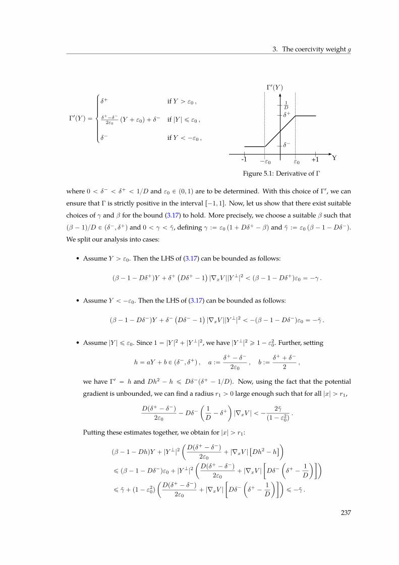
3. The coercivity weight g
Γ1pY q “
$
’
’
’
’
’
’
&
’
’
’
’
’
’
%
δ` if Y ą ε0 ,
δ`´δ´
2ε0pY ` ε0q ` δ
´ if |Y | ď ε0 ,
δ´ if Y ă ´ε0 ,
-1 +1´ε0 ε0
1D
δ`
δ´
Γ1pY q
Y
Figure 5.1: Derivative of Γ
where 0 ă δ´ ă δ` ă 1D and ε0 P p0, 1q are to be determined. With this choice of Γ1, we can
ensure that Γ is strictly positive in the interval r´1, 1s. Now, let us show that there exist suitable
choices of γ and β for the bound (3.17) to hold. More precisely, we choose a suitable β such that
pβ ´ 1qD P pδ´, δ`q and 0 ă γ ă γ, defining γ :“ ε0 p1`Dδ` ´ βq and γ :“ ε0 pβ ´ 1´Dδ´q.
We split our analysis into cases:
• Assume Y ą ε0. Then the LHS of (3.17) can be bounded as follows:
pβ ´ 1´Dδ`qY ` δ``
Dδ` ´ 1˘
|∇xV ||YK|2 ă pβ ´ 1´Dδ`qε0 “ ´γ .
• Assume Y ă ´ε0. Then the LHS of (3.17) can be bounded as follows:
pβ ´ 1´Dδ´qY ` δ´`
Dδ´ ´ 1˘
|∇xV ||YK|2 ă ´pβ ´ 1´Dδ´qε0 “ ´γ .
• Assume |Y | ď ε0. Since 1 “ |Y |2 ` |Y K|2, we have |Y K|2 ě 1´ ε20. Further, setting
h “ aY ` b P pδ´, δ`q , a :“ δ` ´ δ´
2ε0, b :“ δ` ` δ´
2 ,
we have Γ1 “ h and Dh2 ´ h ď Dδ´pδ` ´ 1Dq. Now, using the fact that the potential
gradient is unbounded, we can find a radius r1 ą 0 large enough such that for all |x| ą r1,
Dpδ` ´ δ´q
2ε0´Dδ´
ˆ
1D´ δ`
˙
|∇xV | ă ´2γ
p1´ ε20q.
Putting these estimates together, we obtain for |x| ą r1:
pβ ´ 1´DhqY ` |Y K|2ˆ
Dpδ` ´ δ´q
2ε0` |∇xV |
“
Dh2 ´ h‰
˙
ď pβ ´ 1´Dδ´qε0 ` |YK|2
ˆ
Dpδ` ´ δ´q
2ε0` |∇xV |
„
Dδ´ˆ
δ` ´1D
˙˙
ď γ ` p1´ ε20q
ˆ
Dpδ` ´ δ´q
2ε0` |∇xV |
„
Dδ´ˆ
δ` ´1D
˙˙
ď ´γ .
237
5. Fibre lay-down model
# Step 4: Choice of parameters.
We now come back to the choice of δ´, δ`, ε0, β such that κβ ă γ and 0 ă γ ă γ hold true.
More precisely, these two constraints translate into the following bound on β:
1`Dˆ
δ` ` δ´
2
˙
ă β ă
ˆ
ε0
κ` ε0
˙
`
1`Dδ`˘
. (3.18)
It is easy to see that this bound also implies 1 ` Dδ´ ă β ă 1 ` Dδ` as required. However, for
this to be possible we need to choose ε0 such that LHS ă RHS, in other words,
κ
ˆ
2`D pδ` ` δ´qD pδ` ´ δ´q
˙
ă ε0 . (3.19)
Since ε0 has to be less than 1 andDpδ`´ δ´qp2`D pδ` ` δ´qq ă 13, this bound is only possible
if κ P p0, 13q; then it remains to choose 0 ă δ´ ă δ` ă 1D such that
κ ăD pδ` ´ δ´q
2`D pδ` ` δ´q Pˆ
0, 13
˙
. (3.20)
To satisfy all these constraints, we make the choice of parameters (for κ ă 13):
δ` :“ 3p1` κq4D , δ´ :“ p1´ 3κq
4D .
Then (3.20) holds true, and we can fix ε0 P p0, 1q to satisfy (3.19):
ε0 :“ 12
ˆ
1` κˆ
2`D pδ` ` δ´qD pδ` ´ δ´q
˙˙
“12
ˆ
1` 9κ1` 3κ
˙
.
Finally, we choose β satisfying (3.18) as follows:
β :“ 12
„
1`Dˆ
δ` ` δ´
2
˙
`
ˆ
ε0
κ` ε0
˙
`
1`Dδ`˘
“34 `
p1` 9κqp7` 3κq8p6κ2 ` 11κ` 1q P p1, 2q .
4 Existence and uniqueness of a steady state
4.1 Existence of a C0-semigroup
Proving existence of solutions to the perturbed equation (1.2) relies on the a priori estimates from
Section 2:
Theorem 4.1. The linear operator Lκ : DpLκq Ñ L2pdµκq defined in (1.5) is the infinitesimal generator
of a C0-semigroup pStqtě0 on L2pdµκq.
Proof. Let us denote by L˚κ the adjoint of Lκ in L2pdµκq. Both domains D pLκq and D pL˚κq contain
the core C and are dense. The operator Lκ is closable in L2pdµκq. To see this, take a sequence
238
4. Existence and uniqueness of a steady state
pfnqnPN P DpLκq converging to zero in L2pdµκq such that the sequence pLκfnqnPN converges to
some limit h P L2pdµκq. Then for any test function ϕ P C,
@
ϕ , LκfnD
κ“@
L˚κϕ , fnD
κÑ 0 as nÑ8 .
Since the left-hand side converges to@
ϕ , hD
κfor all ϕ P C, we conclude h ” 0 a.e., and so Lκ is
closable. Similarly, L˚κ is closable. We denote by Lκ and L˚κ some closed extensions of Lκ and L˚κ,
respectively. Lumer-Phillips Theorem in the form [254, Corollary 4.4] states that an operator L
generates a C0-semigroup if L is closed and both L and L˚ are dissipative. Since the core C is dense
in both DpQκq and DpQ˚κq, which in turn are both dense in L2pdµκq, then for any constant C ą 0,
Lκ ´ CId is dissipative if and only if L˚κ ´ CId is dissipative. Therefore, it remains to show that
Lκ ´ CId is dissipative for some C ą 0. Since the restriction of Lκ to C is Lκ, it is enough to prove
that Lκ ´ CId is dissipative on C for some constant C ą 0. The estimates in Section 2 show that
there exists C ą 0 s.t.
@f P C,@
Lκf , fD
κď Cf2κ
for some explicit constant C ą 0, which concludes the proof.
4.2 Proof of Theorem 1.4
Proposition 2.1 is the key ingredient to deduce existence of a unique steady state. The set
B :“"
f P L2pdµκq : Grf s ď γ2
γ1, f ě 0, Mf “ 1
*
is convex and bounded in L2pdµκq by the norm equivalence (2.9). By Theorem 4.1, the operator Lκgenerates a C0-semigroup pStqtě0. Then let us show that B is invariant under the action of pStqtě0.
Integrating in time the hypocoercivity estimate (2.10) in Proposition 2.1 for any fin P L2pdµκqwith
mass 1, we obtain the bound
Grfptqs ď Grfinse´γ1t `γ2
γ1
`
1´ e´γ1t˘
,
and thus
@ t ą 0, Grfptqs ď max"
Grfins,γ2
γ1
*
.
Since in addition, pStqtě0 conserves mass and positivity, we conclude StpBq Ă B for all times.
Integrate again the hypocoercivity estimate (2.10) in Proposition 2.1, now for the difference of
two solutions with same mass, to get
GrStf ´ Sths ď e´γ1tGrf ´ hs
for any t ą 0 and f, h P B. It follows by Banach’s fixed-point theorem that there exists a unique
ut P B such that Stputq “ ut for each t ą 0. Let tn :“ 2´n, n P N, and un :“ utn . Then S2´npunq “
239
5. Fibre lay-down model
un, and by repeatedly applying the semigroup property,
@ k P N, @m ď n P N, Sk2´mpunq “ un . (4.21)
Let us prove that B is weakly compact in L2pdµκq. Consider a sequence pfnqnPN P B. It has a
cluster point f for the weak convergence since B is bounded in L2pdµκq, and the corresponding
subsequence is still denoted fn for simplicity. By lower semi-continuity of the equivalent norm G:
Grf s ď lim infnÑ8
Grfns ď γ2γ1 .
Further, since fn ě 0 for all n P N, it follows that f ě 0 (the set of non-negative functions is a
strongly closed convex set, hence weakly closed). It remains to show that the limit f has mass 1 by
preventing loss of mass at infinity. Use Cauchy-Schwarz’s inequality and the norm equivalence
(2.9) to get for r ą 0
p1` κζq˜
ż
|x|ąr
Πfn dx¸2
ď
˜
ż
|x|ąr
ż
S1f2n e
V dxdα2π
¸˜
ż
|x|ąr
ż
S1e´V
dxdα2π
¸
` κζ
˜
ż
|x|ąr
ż
S1f2n g
dxdα2π
¸˜
ż
|x|ąr
ż
S1g´1 dxdα
2π
¸
ď fn2κ
˜
ż
|x|ąr
ż
S1
`
e´V ` g´1˘ dxdα2π
¸
ď
ˆ
21´ ε1
˙
γ2
γ1
˜
ż
|x|ąr
ż
S12e´V dxdα
2π
¸
.
This shows that
supnPN
˜
ż
|x|ąr
Πfn dx¸
ď
ˆˆ
4p1´ ε1qp1` κζq
˙ˆ
γ2
γ1
˙˙12˜
ż
|x|ąr
ż
S1e´V
dxdα2π
¸12
Ñ 0 as r Ñ8 ,
sinceş
R2ˆS1 e´V dxdα
2π “ 1. Together with Mfn “ 1 for all n P N, it follows that Mf “ 1. Hence
f P B. The weak compactness of B implies the existence of a subsequence unj of un and a function
u P B such that unj converges weakly to u in L2pdµκq. Letting nj Ñ8 in (4.21) implies that (since
St is a continuous operator)
@m P N, @ k P N, Sk2´mpuq “ u .
Finally the density of the dyadic rationals tk2´m : k P N,m P Nu in p0,`8q and continuity of Stpuq
in t for all u P B imply that
@ t ě 0, Stpuq “ u .
This shows the existence and uniqueness of a global stationary state Fκ :“ u P B.
240
4. Existence and uniqueness of a steady state
To complete the proof of Theorem 1.4, we apply the hypocoercivity estimate Proposition 2.1 to
the difference between a solution f P L2pdµκq and the unique stationary state of the same mass,
MfFκ, to show exponential convergence to equilibrium in ¨ κ: first of all, we deduce from the
contraction estimate (2.10) that
Grfptq ´MfFκs ď Grfin ´MfFκs e´γ1t ,
which allows then to estimate the difference to equilibrium in theL2pdµκq-norm. Indeed, by norm
equivalence, we obtain
fptq ´MfFκ2κ ď
1` ε1
1´ ε1fin ´MfFκ
2κ e´γ1t .
Hence, we obtain (1.8) with rate of convergence λκ :“ γ12.
Remark 4.2. From our previous estimates, we have that GpFkq is uniformly bounded in κ for κ sufficiently
small. As a consequence, pFκqκą0 is a relatively weakly compact family in L2pdµκq, and by uniqueness of
the stationary state in the case κ “ 0, we deduce that Fκ Ñ F0 as κ Ñ 0. It could also be proved with
further work that the optimal (spectral gap) relaxation rate is continuous as κÑ 0.
241

Part III
Scaling Approaches for Social Dynamics
243

Thinking Fluids
Do you remember the last time you saw birds in the sky?
Thousands of birds, moving in coordinated patterns?
Often, each bird can only see the birds right next to it,
and yet they manage to create an emerging collective behaviour.
How do they do it?
What if we consider that each bird is reacting according to 3 simple rules:
1. Repulsion – they don’t want to be too close to each other,
2. Attraction – they don’t want to loose the group,
3. Alignment – they want to go in the same direction as their neighbours.
If we put these 3 simple rules into a mathematical model,
we can recreate the same patterns that we observe in nature.
Now, why should we care about birds?
In fact, what matters is
how we can predict the behaviour of a large group of individuals
by knowing only how each one of them reacts to its neighbours.
Imagine zooming out and looking at many many birds from far away,
it looks like a continuous fluid.
Mathematically,
this can be described by a partial differential equation,
or PDE.
PDEs encode the physical laws about how a quantity changes with
time, position and velocity.
Often, these models are so complicated,
that there is no hope of finding explicit solutions.
However, sometimes,
we are able to read the important properties from the model itself.
My research is about proving these properties
and trying to explain the longterm behaviour of solutions
without knowing these solutions explicitly.
The exact same PDE that models the behaviour of birds
can also model many other organisms
from schools of fish, to colonies of bacteria.
245
But what about us humans?
You would think that
human communication is far too complicated
to be reduced into function,
right?
Well, actually, in certain situations,
people react instinctively,
and we can use the same type of PDE
to model the motion of pedestrian crowds.
A famous example of dangerous overcrowding
is the Jamarat Bridge in Saudi-Arabia,
where hundreds died during pilgramage.
We can model these disasters
by treating the crowd as a thinking fluid,
just like birds, fish or bacteria.
This will allow us to make predictions for panic situations
such as earthquakes and fire escapes,
and hopefully it will help us
to prevent crowd disasters in the future.
What is so fascinating
is that all these different applications
are just special cases of the same class of PDEs.
If we understand more about the general structure of these models,
we will have added a timeless piece of wisdom
to our understanding of the world.
Text for 3-Minute-Thesis Competition
by Franca Hoffmann
Imperial College London, April 2016
246
Chapter6
Non-local models for
self-organised animal aggregation
This chapter follows in most parts the article “Non-local kinetic and macroscopic models for self-
organised animal aggregations” written in collaboration with José A. Carrillo1 and Raluca Ef-
timie2, and published in Kinetic and Related Models 8 (2015), no. 3, 413 - 441. Section 2.2 was
contributed by Raluca Eftimie and Section 3.2 was contributed by José A. Carrillo. Some of the
results presented in this chapter were already part of my master thesis, namely: (1) a special case
of the parabolic scaling for the kinetic 1D model (2.1) under assumption (2.14) with λ1 “ 0 (Re-
mark 2.2), (2) the parabolic drift-diffusion limit of the 2D kinetic model (3.18) with λ1 “ 0 (Section
3.1), and (3) a theoretical development of the AP scheme (Section 4) for the 1D kinetic model (2.1)
under scaling assumption (2.14) with λ1 “ 0. These parts have been included here to allow for a
comprehensive and self-contained presentation of the chapter.
Chapter Summary
The last two decades have seen a surge in kinetic and macroscopic models derived to inves-
tigate the multi-scale aspects of self-organised biological aggregations. Because the individual-
level details incorporated into the kinetic models (e.g., individual speeds and turning rates)
make them somewhat difficult to investigate, one is interested in transforming these models
into simpler macroscopic models, by using various scaling techniques that are imposed by the
biological context. However, not many studies investigate how the dynamics of the initial mod-
els are preserved via these scalings. Here, we consider two scaling approaches (parabolic and
grazing collision limits) that can be used to reduce a class of non-local 1D and 2D models for
biological aggregations to simpler models existent in the literature. Then, we investigate how
some of the spatio-temporal patterns exhibited by the original kinetic models are preserved via
1Department of Mathematics, Imperial College London, South Kensington Campus, London SW7 2AZ, UK.2Division of Mathematics, University of Dundee, Dundee, UK.
247
6. Self-organised animal aggregation
these scalings. To this end, we focus on the parabolic scaling for non-local 1Dmodels and apply
asymptotic preserving numerical methods, which allow us to analyse changes in the patterns as
the scaling coefficient ε is varied from ε “ 1 (for 1D transport models) to ε “ 0 (for 1D parabolic
models). We show that some patterns (describing stationary aggregations) are preserved in the
limit ε Ñ 0, while other patterns (describing moving aggregations) are lost. To understand the
loss of these patterns, we construct bifurcation diagrams.
Chapter Content
1 Introduction . . . . . . . . . . . . . . . . . . . . . . . . . . . . . . . . . . . . . . . 249
2 Description of 1D models . . . . . . . . . . . . . . . . . . . . . . . . . . . . . . . 251
2.1 Parabolic limit for non-linear interactions . . . . . . . . . . . . . . . . . . 255
2.2 The preservation of steady states and their stability as ε Ñ 0 . . . . . . 257
3 Description of 2D models . . . . . . . . . . . . . . . . . . . . . . . . . . . . . . . 260
3.1 Parabolic drift-diffusion limit . . . . . . . . . . . . . . . . . . . . . . . . 263
3.2 Grazing collision limit . . . . . . . . . . . . . . . . . . . . . . . . . . . . 267
4 Asymptotic preserving methods for 1D models . . . . . . . . . . . . . . . . . . . 270
4.1 Odd and even parity . . . . . . . . . . . . . . . . . . . . . . . . . . . . . 270
4.2 Operator splitting . . . . . . . . . . . . . . . . . . . . . . . . . . . . . . . 271
4.3 Alternated upwind discretisation . . . . . . . . . . . . . . . . . . . . . . 271
4.4 Simulation results . . . . . . . . . . . . . . . . . . . . . . . . . . . . . . . 272
5 Summary and discussion . . . . . . . . . . . . . . . . . . . . . . . . . . . . . . . 274
Milima haikutani,
lakini binadamu hukutana.
Mountains don’t meet,
but human beings do3.
Kiswahili Proverb
3Do not say that you will never meet somebody.
248
1. Introduction
1 Introduction
Over the past 10-20 years a multitude of kinetic and macroscopic models have been introduced
to investigate the formation and movement of various biological aggregations: from cells [22, 5]
and bacteria [257] to flocks of birds, schools of fish and even human aggregations (see, for exam-
ple, [290, 83, 251, 86, 124, 27, 112] and the references therein). The use of kinetic or macroscopic
approaches is generally dictated by the problem under investigation: (i) kinetic (transport) mod-
els focus on changes in the density distribution of individuals that have a certain spatial position,
speed and movement direction (or are in some activity state [24]); (ii) macroscopic models focus
on changes in the averaged total density of individuals [87, 144].
Generally, these kinetic and macroscopic models assume that individuals, particles, or cells
can organise themselves in the absence of a leader. The factors that lead to the formation of self-
organised aggregations are the interactions among individuals as a result of various social forces:
repulsion from nearby neighbours, attraction to far-away neighbours (or to roosting areas [93])
and alignment/orientation with neighbours positioned at intermediate distances. These interac-
tion forces are usually assumed to act on different spatial ranges, depending on the communica-
tion mechanisms used by individuals; e.g., via acoustic long-range signals, or via chemical/visual
short-range signals. The non-locality of the attractive and alignment/orientation interactions is
supported by radar tracking observations of flocks of migratory birds, which can move with the
same speed and in the same direction despite the fact that individuals are 200-300 meters apart
from each other [209]. For the repulsive forces some models consider non-local effects gener-
ated by decaying interactions with neighbours positioned further and further away [146], while
other models consider only local effects [282]. In the case of continuous mesoscopic and macro-
scopic models, the non-local interactions are modelled by interaction kernels (see Figure 6.1 for
2D and 1D kernels). The most common choices for these kernels are Morse potential-type ker-
nels [87, 83, 86, 91] (see Figure 6.1(b)) and Gaussian kernels [147, 146, 144, 237] (see Figure 6.1(c)).
Due to their complex structure, kinetic models are difficult to investigate. Although progress
has been made in recent years, mainly regarding the existence and stability of various types of
solutions and the analytic asymptotic methods that allow transitions from kinetic (mesoscopic) to
macroscopic models (see, for example, [189, 190, 23, 83, 59, 124, 123, 42, 28, 179] and the references
therein), it is still difficult to study analytically and numerically the spatial and spatio-temporal
aggregation patterns exhibited by the kinetic models. For example, there are very few studies that
investigate the types of spatio-temporal patterns obtained with 2D and 3D kinetic models (see the
review in [144]). Moreover, the presence of non-local interaction terms increases the complexity
of the models, leading to a larger variety of patterns that are more difficult to analyse. While
249
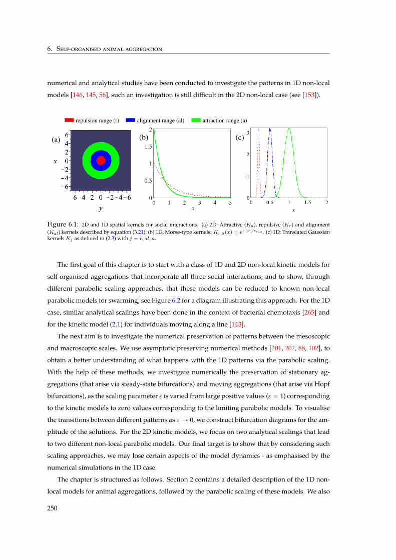
6. Self-organised animal aggregation
numerical and analytical studies have been conducted to investigate the patterns in 1D non-local
models [146, 145, 56], such an investigation is still difficult in the 2D non-local case (see [153]).
repulsion range (r)
(a)
x
(c)(b)
x
alignment range (al) attraction range (a)
Figure 6.1: 2D and 1D spatial kernels for social interactions. (a) 2D: Attractive (Ka), repulsive (Kr) and alignment(Kal) kernels described by equation (3.21); (b) 1D: Morse-type kernels: Kr,apxq “ e´|x|sr,a . (c) 1D: Translated GaussiankernelsKj as defined in (2.3) with j “ r, al, a.
The first goal of this chapter is to start with a class of 1D and 2D non-local kinetic models for
self-organised aggregations that incorporate all three social interactions, and to show, through
different parabolic scaling approaches, that these models can be reduced to known non-local
parabolic models for swarming; see Figure 6.2 for a diagram illustrating this approach. For the 1D
case, similar analytical scalings have been done in the context of bacterial chemotaxis [265] and
for the kinetic model (2.1) for individuals moving along a line [143].
The next aim is to investigate the numerical preservation of patterns between the mesoscopic
and macroscopic scales. We use asymptotic preserving numerical methods [201, 202, 88, 102], to
obtain a better understanding of what happens with the 1D patterns via the parabolic scaling.
With the help of these methods, we investigate numerically the preservation of stationary ag-
gregations (that arise via steady-state bifurcations) and moving aggregations (that arise via Hopf
bifurcations), as the scaling parameter ε is varied from large positive values (ε “ 1) corresponding
to the kinetic models to zero values corresponding to the limiting parabolic models. To visualise
the transitions between different patterns as εÑ 0, we construct bifurcation diagrams for the am-
plitude of the solutions. For the 2D kinetic models, we focus on two analytical scalings that lead
to two different non-local parabolic models. Our final target is to show that by considering such
scaling approaches, we may lose certain aspects of the model dynamics - as emphasised by the
numerical simulations in the 1D case.
The chapter is structured as follows. Section 2 contains a detailed description of the 1D non-
local models for animal aggregations, followed by the parabolic scaling of these models. We also
250
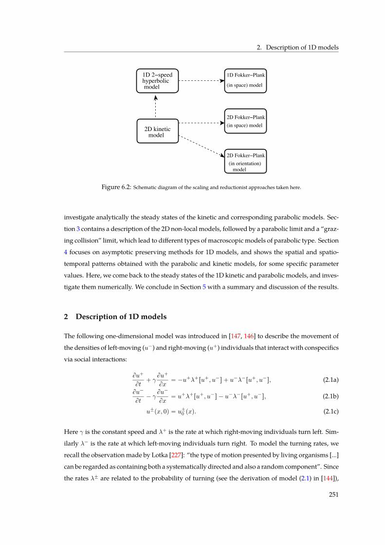
2. Description of 1D models
(in space) model
1D FokkerïPlank
(in space) model
2D FokkerïPlank(in orientation)
model
2D FokkerïPlank<+ /q=
f(y)=y
model2D kinetic
1D 2ïspeed
modelhyperbolic
Figure 6.2: Schematic diagram of the scaling and reductionist approaches taken here.
investigate analytically the steady states of the kinetic and corresponding parabolic models. Sec-
tion 3 contains a description of the 2D non-local models, followed by a parabolic limit and a “graz-
ing collision” limit, which lead to different types of macroscopic models of parabolic type. Section
4 focuses on asymptotic preserving methods for 1D models, and shows the spatial and spatio-
temporal patterns obtained with the parabolic and kinetic models, for some specific parameter
values. Here, we come back to the steady states of the 1D kinetic and parabolic models, and inves-
tigate them numerically. We conclude in Section 5 with a summary and discussion of the results.
2 Description of 1D models
The following one-dimensional model was introduced in [147, 146] to describe the movement of
the densities of left-moving (u´) and right-moving (u`) individuals that interact with conspecifics
via social interactions:
Bu`
Bt` γ
Bu`
Bx“ ´u`λ`ru`, u´s ` u´λ´ru`, u´s, (2.1a)
Bu´
Bt´ γ
Bu´
Bx“ u`λ`ru`, u´s ´ u´λ´ru`, u´s, (2.1b)
u˘px, 0q “ u˘0 pxq. (2.1c)
Here γ is the constant speed and λ` is the rate at which right-moving individuals turn left. Sim-
ilarly λ´ is the rate at which left-moving individuals turn right. To model the turning rates, we
recall the observationmade by Lotka [227]: “the type of motion presented by living organisms [...]
can be regarded as containing both a systematically directed and also a randomcomponent”. Since
the rates λ˘ are related to the probability of turning (see the derivation of model (2.1) in [144]),
251
6. Self-organised animal aggregation
they are positive functions defined as:
λ˘ru`, u´s “λ1 ` λ2fpyN ru`, u´sq ` λ3fpy
˘Dru
`, u´sq (2.2)
“λ1 ` λ3
´
λ02fpyN ru
`, u´sq ` fpy˘Dru`, u´sq
¯
,
where we denote by u “ u` ` u´ the total population density and all other terms will be defined
below. In this chapter, we generalise the turning rates in [147, 146, 144] and assume that:
• individuals can turn randomly at a constant rate approximated by λ1 [147];
• individuals can turn randomly in response to the perception of individuals inside any of
the repulsive/attractive/alignment ranges (and independent of the movement direction of
their neighbours). These non-directed interactionswith neighbours are described by the term
yN ru`, u´swith turning rate λ2;
• individuals can turn in response to interactions with neighbours positioned within the re-
pulsive (r), attractive (a) and alignment (al) zones, respectively (see Figure 6.1(a)) [147]. This
turning is directed towards or away from neighbours, depending on the type of interaction (at-
tractive or repulsive). For alignment interactions, individuals turn to move in the same di-
rection as their neighbours. The non-local directed interactionswith neighbours are described
by terms y˘Dru`, u´swith turning rate λ3.
If λ3 ‰ 0, we denote by λ02 the quotient of the turning rates λ2λ3. This choice of notation is
motivated by the corresponding 2Dmodel (Section 3). The connection between the 1Dmodel (2.1)
and the 2Dmodel (3.18) will be made clearer in Remarks 3.1, 3.2, 3.3 and 3.4. The turning function
fp¨q is a non-negative, increasing, bounded functional of the interactions with neighbours. An
example of such function is fpY q “ 0.5`0.5 tanhpY ´y0q (see [146]), where y0 is chosen such that
when Y “ 0 (i.e., no neighbours around), then fp0q « 0 and the turning is mainly random.
To model the long-distance social interactions that lead to turning behaviours, we define the
interaction kernels in 1D, see Figure 6.1, as decreasing functions of the distance between the ref-
erence position x (of the population density) and the mid of the interaction ranges sj , j “ r, al, a,
Kjpxq “1
b
2πm2j
e´px´sjq2p2m2
j q, (2.3)
for x ą 0 and zero otherwise, with j “ r, al, a denoting short-range repulsion (Kr), medium-range
alignment (Kal) and long-range attraction (Ka) interaction kernels. Here, mj “ sj8 controls the
width of the interaction range j.
For the non-directeddensity-dependent turningwedefine the turning kernel,KN pxq “ KN pxq`
KN p´xqwith KN “ qrKr` qalKal` qaKa obtained by superimposing the kernelsKj , j “ r, al, a.
252
2. Description of 1D models
Here qr, qal and qa represent the magnitudes of the repulsive, alignment and attractive social in-
teractions. Note that in [146], λ02 “ 0 and the density-dependent non-directed turning term does
not exist. However, in 2D, this term appears naturally when we incorporate random turning be-
haviour (as discussed in Section 3). With these notations we may define
yN rus “ KN ˚ u, with u “ u` ` u´,
for the non-directed turning mechanisms. We assume here that individuals turn randomly when-
ever theyperceive other neighbours around (within the repulsive, alignment and attractive ranges).
For the directed density-dependent turning, we define
y˘Dru`, u´s “ y˘r ru
`, u´s ´ y˘a ru`, u´s ` y˘alru
`, u´s. (2.4)
Here, y˘j ru`, u´s, j “ r, al, a, describe the directed turning in response to neighbours within the
repulsive (r), alignment (al) and attractive (a) social ranges (as in [147]). Aswewill explain shortly,
the direction of the turning will be given by incorporating movement direction towards or away
conspecifics. For this reason, y˘a and y˘r enter equation (2.4) with opposite signs.
The density-dependent turnings depend greatly on how individuals communicate with each
other, namely whether they can emit (perceive) signals to (from) all or some of their neighbours.
Two particular situations, described by models called M2 and M4 as in [146] (see Figure 6.3) are
considered:
• Model M2: Individuals communicate via omni-directional communication signals, and thus
they can perceive all their neighbours positioned around them within all social interaction
ranges. For instance, the majority of mammals communicate via a combination of visual,
chemical and auditory signals, which allows them to receive/send information from/to all
their neighbours. With this assumption (see Figure 6.3(a)), the terms y˘r,a,al are defined as
follows:
y˘r,aru`, u´s “ qr,a
ż 8
0Kr,apsq
`
upx˘ sq ´ upx¯ sq˘
ds, (2.5a)
y˘alru`, u´s “ qal
ż 8
0Kalpsq
`
u¯px¯ sq ` u¯px˘ sq (2.5b)
´u˘px¯ sq ´ u˘px˘ sq˘
ds.
Here, qj describe the magnitudes of the social interactions associated to the interaction ker-
nels defined in (2.3). To understand the effect of these terms on the turning rates, let us focus
on y`r , for example. If upx ` sq ą upx ´ sq, then y`r enters λ` with positive sign, suggest-
ing a higher likelihood of turning, to avoid collision with neighbours ahead at x ` s. If, on
253
6. Self-organised animal aggregation
the other hand, upx ` sq ă upx ´ sq, then y`r enters λ` with a negative sign, suggesting a
lower likelihood of turning. In this case, the individuals at x will keep moving in the same
direction, to avoid collision with neighbours behind at x ´ s. Note that the directionality
of neighbours influences only the alignment interactions (the attractive and repulsive inter-
actions being defined in terms of the total density u). Also, for this particular model, the
random density-dependent terms are given by
yN rus “
ż 8
0KN psq
`
upx` sq ` upx´ sqqds. (2.6)
• Model M4: Individuals communicate via unidirectional communication signals, and thus
they can perceive only those neighbours moving towards them. For example, birds commu-
nicate via directional sound signals, and to ensure an effective transmission of their signals
they orient themselves towards their targeted receivers [52]. With this assumption (see Fig-
ure 6.3(b)), the terms y˘r,a,al are defined as follows:
y˘r,a,alru`, u´s “ qr,a,al
ż 8
0Kr,a,alpsq
`
u¯px˘ sq ´ u˘px¯ sq˘
ds. (2.7)
Here, the directionality of neighbours influences all three social interactions. Moreover, for
this model, the random density-dependent terms are given by
yN ru`, u´s “
ż 8
0KN psq
`
u´px` sq ` u`px´ sqqds. (2.8)
In this equation, we assume that individuals turn randomly in response to u´ and u` in-
dividuals (i.e., in (2.8) we add all perceived individuals; this is in contrast to equation (2.7),
where we subtract individuals positioned ahead from individuals positioned behind, to im-
pose directionality in the turning behaviour). Note that in (2.8), yN does not depend any-
more on u “ u` ` u´ (as in (2.6)), since the individuals at x cannot perceive all their neigh-
bours at x˘ s.
We focus on these two particular models because: (i) the model (2.1)+(2.2)+(2.5)+(2.6) assum-
ing λ1 “ 0 has been generalised to 2D; (ii) the model (2.1)+(2.2)+(2.7)+(2.8) assuming λ2 “ 0 has
been investigated analytically and numerically, and showed that it can exhibit Hopf bifurcations
(even when qal “ 0), which give rise to spatio-temporal patterns such as rotating waves and mod-
ulated rotating waves [56]. In contrast, model (2.1)+(2.2)+(2.5)+(2.6) with λ2 “ 0 does not seem to
exhibit rotating waves when qal “ 0, see [146].
To complete the description of themodel, we need to specify the domain size and the boundary
conditions. Throughout most of this chapter, we will consider an infinite domain. However, for
the purpose of numerical simulations, in Sections 2.2 and 4 we will consider a finite domain of
length L (i.e., r0, Ls) with periodic boundary conditions: u`pL, tq “ u`p0, tq, u´p0, tq “ u´pL, tq.
254
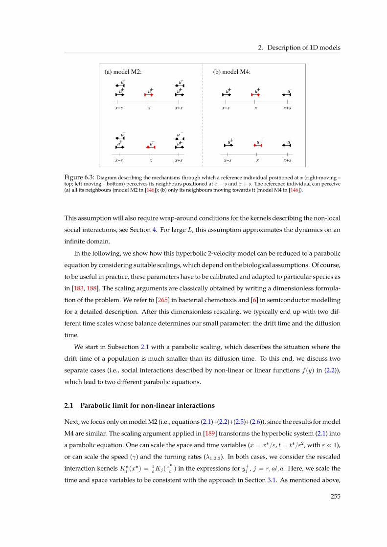
2. Description of 1D models
x+sxïs
xïs x x+s xïs
x
x x+s
xxïs x+s
+uu
uu+ + u
(a) model M2: (b) model M4:
u+ u+
u+u u
uuuu++u
u
Figure 6.3: Diagram describing the mechanisms through which a reference individual positioned at x (right-moving –top; left-moving – bottom) perceives its neighbours positioned at x ´ s and x ` s. The reference individual can perceive(a) all its neighbours (model M2 in [146]); (b) only its neighbours moving towards it (model M4 in [146]).
This assumptionwill also require wrap-around conditions for the kernels describing the non-local
social interactions, see Section 4. For large L, this assumption approximates the dynamics on an
infinite domain.
In the following, we show how this hyperbolic 2-velocity model can be reduced to a parabolic
equation by considering suitable scalings, which depend on the biological assumptions. Of course,
to be useful in practice, these parameters have to be calibrated and adapted to particular species as
in [183, 188]. The scaling arguments are classically obtained by writing a dimensionless formula-
tion of the problem. We refer to [265] in bacterial chemotaxis and [6] in semiconductor modelling
for a detailed description. After this dimensionless rescaling, we typically end up with two dif-
ferent time scales whose balance determines our small parameter: the drift time and the diffusion
time.
We start in Subsection 2.1 with a parabolic scaling, which describes the situation where the
drift time of a population is much smaller than its diffusion time. To this end, we discuss two
separate cases (i.e., social interactions described by non-linear or linear functions fpyq in (2.2)),
which lead to two different parabolic equations.
2.1 Parabolic limit for non-linear interactions
Next, we focus only onmodelM2 (i.e., equations (2.1)+(2.2)+(2.5)+(2.6)), since the results formodel
M4 are similar. The scaling argument applied in [189] transforms the hyperbolic system (2.1) into
a parabolic equation. One can scale the space and time variables (x “ x˚ε, t “ t˚ε2, with ε ! 1),
or can scale the speed (γ) and the turning rates (λ1,2,3). In both cases, we consider the rescaled
interaction kernels K˚j px˚q “ 1εKjp
x˚
ε q in the expressions for y˘j , j “ r, al, a. Here, we scale the
time and space variables to be consistent with the approach in Section 3.1. As mentioned above,
255
6. Self-organised animal aggregation
the scaling parameter ε depends on the biological problem modelled. For example, in [189] the
authors connect ε to the ratio of the drift (τdrift) and diffusion (τdiff ) times observed in bacteria
such as E. coli, where τdrift « 100 seconds and τdiff « 104 seconds, and thus ε « Op10´2q.
Similar scaling arguments are used in [265, Appendix] to analyse the ability of parabolic scalings
to describe travelling pulses.
To perform the scaling, let us re-write model (2.1) in terms of the total density upx, tq and the
flux vpx, tq “ γpu`px, tq ´ u´px, tqq of individuals (see also [189, 192]):
ε2 Bu
Bt` ε
Bv
Bx“ 0, (2.9a)
ε2 Bv
Bt` εγ2 Bu
Bx“ γu
`
λ´ru, vs ´ λ`ru, vs˘
´ v`
λ`ru, vs ` λ´ru, vs˘
, (2.9b)
with initial conditions upx, 0q “ u0pxq, vpx, 0q “ v0pxq. For clarity, here we dropped the ˚ from
the rescaled space (x˚) and time (t˚) variables. In addition, we assume that individuals have a
reduced perception of the surrounding neighbours for small values of ε, [143]:
fε
´
y˘Dru, vs¯
“ εf´
y˘D“
u,
ż
x˚
ε
εBu
Bt˚‰
¯
, fε
´
yN rus¯
“ εf´
yN rus¯
, (2.10)
where f enters the turning functions λ˘ (2.2):
λ`r¨s ` λ´r¨s “ 2λ1 ` 2λ2 εfpyN r¨sq ` ε λ3
´
fpy`Dr¨sq ` fpy´Dr¨sq
¯
,
λ´r¨s ´ λ`r¨s “ λ3ε´
fpy´Dr¨sq ´ fpy`Dr¨sq
¯
.
By eliminating v “ εş
xBuBt from equations (2.9), and taking the limit εÑ 0, we obtain the following
parabolic equationBu
Bt“γ2
2λ1
B
Bx
ˆ
Bu
Bx
˙
´λ3γ
2λ1
B
Bx
``
fpy´Drusq ´ fpy`Drusq
˘
u˘
. (2.11)
We note here that the non-local terms fpy˘Drusq now depend only on the repulsive and attractive
interactions. The reason for this is that the alignment interactions are defined in terms of u˘ “
pu ˘ 1γ vq2 “ 0.5pu ˘ 1
γ
ş
xεε2BuBtq. As ε Ñ 0, the u terms in (2.5) cancel out, and the integrals
approach zero. Equation (2.11) can be re-written asBu
Bt“B
Bx
ˆ
D0Bu
Bx
˙
´B
Bx
´
S0 uV puq¯
, (2.12)
with diffusion rateD0 “ γ2p2λ1q and drift rate S0 “ λ3γp2λ1q. The velocity V puq depends on the
communication mechanism incorporated. For example, for model M2 we have y˘Drus “ ˘K ˚ u,
and so the velocity is given by
V rus “ f`
´K ˚ u˘
´ f`
K ˚ u˘
where we define
K ˚ u “ K` ˚ u´ K´ ˚ u, K˘ ˚ u “
ż 8
0Kpsqupx˘ sqds,
K “ qrKr ´ qaKa. (2.13)
256
2. Description of 1D models
For model M4, we have y˘Drus “ ˘0.5K ˚u, and so the velocity is quite similar: V rus “ f`
´0.5K ˚
u˘
´ f`
0.5K ˚ u˘
, the factor 0.5 appearing from u˘ “ 0.5pu˘ 1γ vq.
Remark 2.1. We observe that the random density-dependent turning fpyN rusq does not appear in this
parabolic limit. This is the result of the scaling assumptions (2.10).
Remark 2.2. Here, the turning functions fp¨q were chosen to be bounded, since individuals cannot turn
infinitely fast when subject to very strong interactions with neighbours [146, 145]. However, for simplicity,
many models consider linear functions: fpzq “ z (see, for example, [237, 239, 153]). The choice of having
bounded or non-bounded turning functions fp¨q has further implications on the models. In particular, for
linear functions, the argument y˘D “ y˘r ´ y˘a ` y˘al can be either positive or negative (depending on
the magnitudes of the social interactions), with y`D “ ´y´D. For very small constant and non-directional
turning rates (λ1, λ2 « 0), this can lead to λ` ă 0 and λ´ ą 0, or vice versa. Now the u`λ` terms add to
the u´λ´ terms, causing both u` and u´ populations to decide very fast to move in the same direction (in
fact, one of the populations is reinforced to keep its moving direction). This is different from the case with
bounded turning functions, where if y`D “ ´y´D ! 0, then 0 ă λ` « λ1 ` λ2f pyN ru
`, u´sq ă λ´. So if
λ1, λ2 « 0, then u`λ` « 0 and hence population u` is not reinforced to keep its movement direction.
Because the 2D kinetic model that we will investigate in Section 3 assumes f to be a linear function, with a
very weak directed turning behaviour (ελ3), we now consider the case fpyN rusq “ yN rus “ KN ˚ u and
fpy˘Drusq “ εy˘Drus, and so the turning rates can be written as
λ˘ru`, u´s “ λ1 ` λ2KN ˚ u` ε λ3y
˘Drus . (2.14)
By taking the limit ε Ñ 0 in (2.9), we obtain the following parabolic equation with density-dependent
coefficients:
Bu
Bt“B
Bx
ˆ
DrusBu
Bx
˙
´B
Bx
´
Srusu`
y´Drus ´ y`Drus
˘
¯
, (2.15a)
Drus “γ2
2pλ1 ` λ2KN ˚ uqand Srus “
λ3γ
2pλ1 ` λ2KN ˚ uq. (2.15b)
This expression is similar to the asymptotic parabolic equation (3.30) for the 2D model. We will return to
this aspect in Section 3.1.
2.2 The preservation of steady states and their stability as ε Ñ 0
The spatially homogeneous steady states describe the situationwhere individuals are evenly spread
over the whole domain. In the following we investigate how these steady states and their linear
stability are preserved in the parabolic limit. To this end, we focus on the more general case of
non-linear social interactions (the case with linear interactions is similar). For simplicity we as-
sume here that λ2 “ 0 and qal “ 0. To calculate these spatially homogeneous states we need to
257
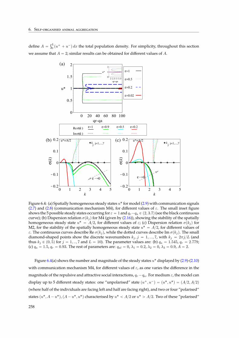
6. Self-organised animal aggregation
define A “şL
0 pu` ` u´q dx the total population density. For simplicity, throughout this section
we assume that A “ 2; similar results can be obtained for different values of A.σ
( )k
u*=A/2u*=A/2j=1,...,7
ε=0.2ε=0.5ε=0.9ε=1Reσ( )k
σ( )kIm
ε 0ε 0
σ(
)k
j j=1,...,7(c)
j
ε=1
ε=0.02
ε=0.2
ε=0.5
(b)
(a)
Figure 6.4: (a) Spatially homogeneous steady states u˚ formodel (2.9) with communication signals(2.7) and (2.8) (communication mechanism M4), for different values of ε. The small inset figureshows the 5 possible steady states occurring for ε “ 1 and qr´qa P p2, 3.7q (see the black continuouscurve); (b) Dispersion relation σpkjq for M4 (given by (2.16)), showing the stability of the spatiallyhomogeneous steady state u˚ “ A2, for different values of ε; (c) Dispersion relation σpkjq forM2, for the stability of the spatially homogeneous steady state u˚ “ A2, for different values ofε. The continuous curves describe Re σpkjq, while the dotted curves describe Im σpkjq. The smalldiamond-shaped points show the discrete wavenumbers kj , j “ 1, ..., 7, with kj “ 2πjL (andthus kj P p0, 5q for j “ 1, .., 7 and L “ 10). The parameter values are: (b) qa “ 1.545, qr “ 2.779;(c) qa “ 1.5, qr “ 0.93. The rest of parameters are: qal “ 0, λ1 “ 0.2, λ2 “ 0, λ3 “ 0.9, A “ 2.
Figure 6.4(a) shows the number andmagnitude of the steady states u˚ displayed by (2.9)-(2.10)
with communication mechanism M4, for different values of ε, as one varies the difference in the
magnitude of the repulsive and attractive social interactions, qr´qa. For medium ε, the model can
display up to 5 different steady states: one “unpolarised” state pu`, u´q “ pu˚, u˚q “ pA2, A2q
(where half of the individuals are facing left and half are facing right), and two or four ”polarised“
states pu˚, A´ u˚q, pA´ u˚, u˚q characterised by u˚ ă A2 or u˚ ą A2. Two of these ”polarised“
258
2. Description of 1D models
states exist only in a very narrow parameter range: e.g., for ε “ 1, they exist when qr´qa P p2, 3.7q.
The other two ”polarised“ states exist for any qr´qa ą 2. For a calculation of the threshold values
of qr ´ qa that ensure the existence of 3 or 5 steady states see [147]. As ε decreases, the magnitude
of the polarised states decreases (i.e., the differences between the number of individuals facing
right and those facing left are decreasing). Moreover, for small ε, these polarised states appear
only when repulsion becomes much stronger than attraction (i.e., qr ´ qa " 10). When ε “ 0
there is only one steady state u˚ “ A2. Since this state exists for all ε ě 0, from now on we will
focus our attention only on this state. Note that for qal “ 0 and for the communicationmechanism
M2 (not shown here), the non-local attractive-repulsive terms vanish, and there is only one steady
state, u˚ “ A2 “ 1, which does not depend on ε.
Models (2.1) and (2.9) do exhibit a large variety of local bifurcations: codimension-1 Steady-
state and Hopf bifurcations [145] as well as codimension-2 Hopf/Hopf, Hopf/Steady-state and
Steady-state/Steady-state bifurcations [56]. Next we focus on the parameter region where two
such bifurcations can occur. We choose a Hopf/steady-state bifurcation for M4 (Figure 6.4(b))
and a steady-state bifurcation for M2 (Figure 6.4(c)), and investigate what happens when ε Ñ 0.
To identify the parameter regions where these bifurcations occur, we consider a finite domain of
length L, and investigate the growth of small perturbations of spatially homogeneous solutions.
We assume u˘9u˚` a˘exppσt` ikjxq, with kj “ 2πjL, j P N`, the discrete wave-numbers, and
|a˘| ! 1. We substitute these solutions into the linearised system (2.9), and by imposing that the
determinant of this system is zero, we obtain the following dispersion relation, which connects σ
(the growth/decay of the perturbations) with the wave-numbers kj :
ε2σ2 ` σp2Lε1 ´Rε2RepK`qq ` γ2k2j ´ γkjR2ImpK`q “ 0, (2.16)
whereLε1 “ λ1`ελ3fp0q,Rε2 “ 2εu˚λ3f1p0q, and K` “ RepK`q`iImpK`q the Fourier transforms
of K` ˚u described in equations (2.13). Note that the wave numbers kj that become unstable (i.e.,
for which Repσpkjqq ą 0) determine, at least for a short time, the number of ”peaks“ j that emerge
in the spatial distribution of the density.
Figure 6.4(b) shows the stability of the spatially homogeneous steady state u˚ “ A2 for model
M4 as given by the dispersion relation (2.16). Even if the wave-numbers kj are discrete (see the
diamond-shaped points on the x-axis of Figure 6.4(b)), we plot σpkjq, j ą 0 as a continuous func-
tion of kj for clarity. To discuss what happens with a Hopf bifurcation as ε Ñ 0, we focus in
Figure 6.4(b) on a parameter space where such a bifurcation occurs (i.e., where Repσpkjqq “ 0
in (2.16)): qa “ 1.545, qr “ 2.779, λ1 “ 0.2, λ2 “ 0, λ3 “ 0.9 and ε “ 1 (see also [57]). For
these parameter values, three modes become unstable at the same time: a steady-state mode k1
(Impσpk1qq “ 0; associated with stationary patterns with 1 peak) and two Hopf modes k4 and k5
(Impσpk4,5qq ą 0; associated with travelling patterns with 4 or 5 peaks). As εÑ 0, the steady-state
259
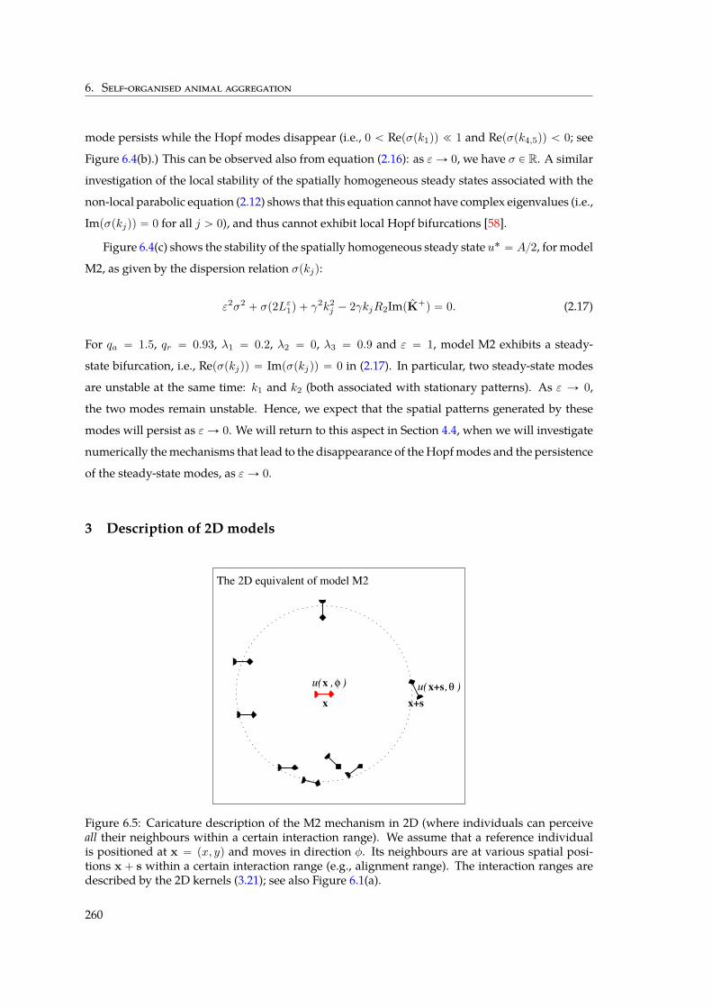
6. Self-organised animal aggregation
mode persists while the Hopf modes disappear (i.e., 0 ă Repσpk1qq ! 1 and Repσpk4,5qq ă 0; see
Figure 6.4(b).) This can be observed also from equation (2.16): as εÑ 0, we have σ P R. A similar
investigation of the local stability of the spatially homogeneous steady states associated with the
non-local parabolic equation (2.12) shows that this equation cannot have complex eigenvalues (i.e.,
Impσpkjqq “ 0 for all j ą 0), and thus cannot exhibit local Hopf bifurcations [58].
Figure 6.4(c) shows the stability of the spatially homogeneous steady state u˚ “ A2, for model
M2, as given by the dispersion relation σpkjq:
ε2σ2 ` σp2Lε1q ` γ2k2j ´ 2γkjR2ImpK`q “ 0. (2.17)
For qa “ 1.5, qr “ 0.93, λ1 “ 0.2, λ2 “ 0, λ3 “ 0.9 and ε “ 1, model M2 exhibits a steady-
state bifurcation, i.e., Repσpkjqq “ Impσpkjqq “ 0 in (2.17). In particular, two steady-state modes
are unstable at the same time: k1 and k2 (both associated with stationary patterns). As ε Ñ 0,
the two modes remain unstable. Hence, we expect that the spatial patterns generated by these
modes will persist as εÑ 0. We will return to this aspect in Section 4.4, when we will investigate
numerically themechanisms that lead to the disappearance of theHopfmodes and the persistence
of the steady-state modes, as εÑ 0.
3 Description of 2D models
x
x
x+s
u( , ) u( , )x+sφ
The 2D equivalent of model M2
θ
Figure 6.5: Caricature description of the M2 mechanism in 2D (where individuals can perceiveall their neighbours within a certain interaction range). We assume that a reference individualis positioned at x “ px, yq and moves in direction φ. Its neighbours are at various spatial posi-tions x` s within a certain interaction range (e.g., alignment range). The interaction ranges aredescribed by the 2D kernels (3.21); see also Figure 6.1(a).
260
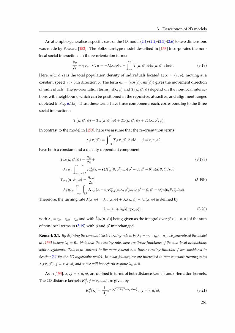
3. Description of 2D models
An attempt to generalise a specific case of the 1Dmodel (2.1)-(2.2)-(2.5)-(2.6) to two dimensions
was made by Fetecau [153]. The Boltzman-type model described in [153] incorporates the non-
local social interactions in the re-orientation terms:
Bu
Bt` γeφ ¨∇xu “ ´λpx, φqu`
ż π
´π
T px, φ1, φqupx, φ1, tqdφ1. (3.18)
Here, upx, φ, tq is the total population density of individuals located at x “ px, yq, moving at a
constant speed γ ą 0 in direction φ. The term eφ “ pcospφq, sinpφqq gives the movement direction
of individuals. The re-orientation terms, λpx, φq and T px, φ1, φq depend on the non-local interac-
tions with neighbours, which can be positioned in the repulsive, attractive, and alignment ranges
depicted in Fig. 6.1(a). Thus, these terms have three components each, corresponding to the three
social interactions:
T px, φ1, φq “ Talpx, φ1, φq ` Tapx, φ1, φq ` Trpx, φ1, φq.
In contrast to the model in [153], here we assume that the re-orientation terms
λjpx, φ1q “ż π
´π
Tjpx, φ1, φqdφ, j “ r, a, al
have both a constant and a density-dependent component:
T alpx, φ1, φq “ηal2π` (3.19a)
λ3 qal
ż π
´π
ż
R2Kdalpx´ sqKo
alpθ, φ1qωalpφ
1 ´ φ, φ1 ´ θqups, θ, tqdsdθ,
T r,apx, φ1, φq “ηr,a2π ` (3.19b)
λ3 qr,a
ż π
´π
ż
R2Kdr,apx´ sqKo
r,aps,x, φ1qωr,apφ1 ´ φ, φ1 ´ ψqups, θ, tqdsdθ.
Therefore, the turning rate λpx, φq “ λalpx, φq ` λapx, φq ` λrpx, φq is defined by
λ “ λ1 ` λ3λrupx, φqs , (3.20)
with λ1 “ ηr`ηal`ηa and with λrupx, φqs being given as the integral over φ1 P r´π, πs of the sum
of non-local terms in (3.19) with φ and φ1 interchanged.
Remark 3.1. By defining the constant basic turning rate to be λ1 “ ηr`ηal`ηa, we generalised the model
in [153] (where λ1 “ 0). Note that the turning rates here are linear functions of the non-local interactions
with neighbours. This is in contrast to the more general non-linear turning function f we considered in
Section 2.1 for the 1D hyperbolic model. In what follows, we are interested in non-constant turning rates
λjpx, φ1q, j “ r, a, al, and so we will henceforth assume λ3 ‰ 0.
As in [153], λj , j “ r, a, al, are defined in terms of both distance kernels and orientation kernels.
The 2D distance kernelsKdj , j “ r, a, al are given by
Kdj pxq “
1Aje´p?x2`y2´djqm
2j , j “ r, a, al, (3.21)
261
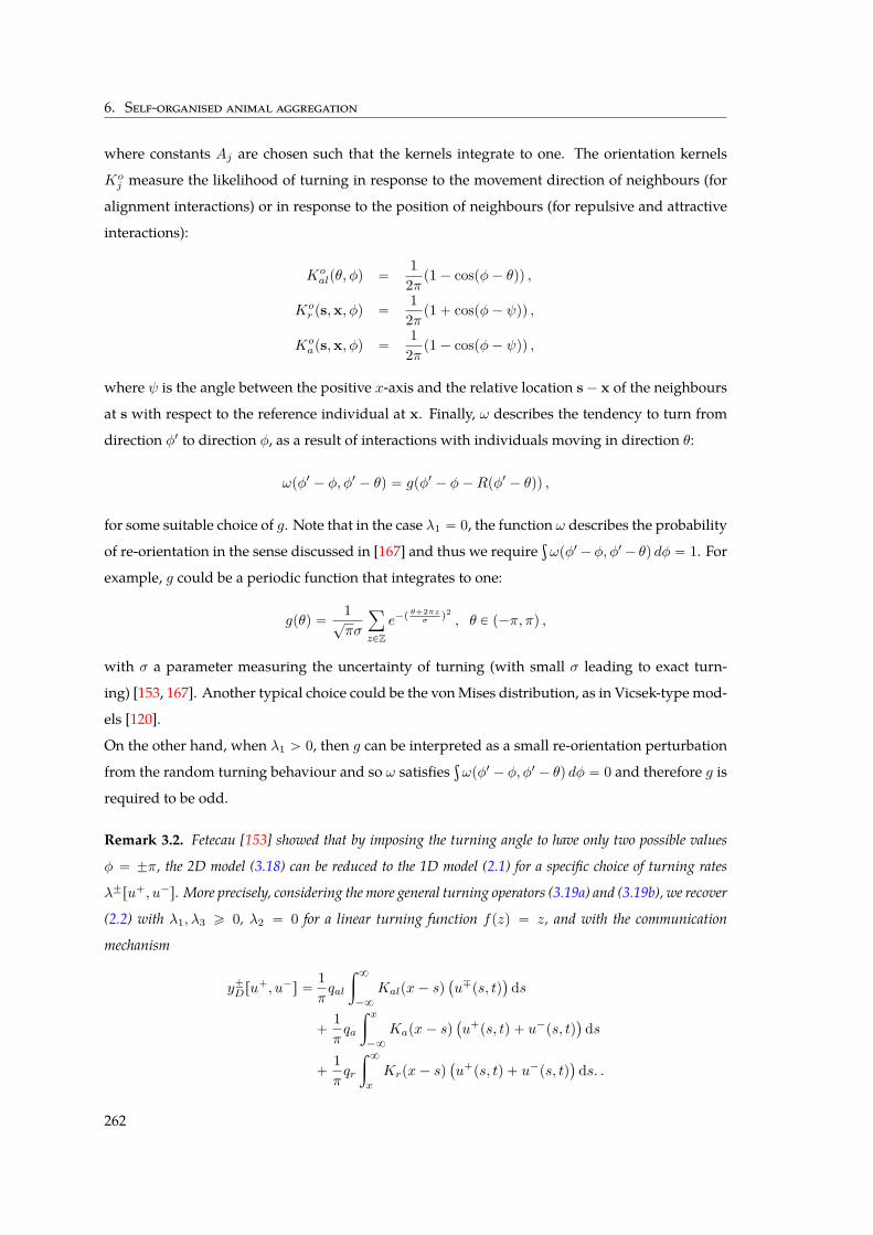
6. Self-organised animal aggregation
where constants Aj are chosen such that the kernels integrate to one. The orientation kernels
Koj measure the likelihood of turning in response to the movement direction of neighbours (for
alignment interactions) or in response to the position of neighbours (for repulsive and attractive
interactions):
Koalpθ, φq “
12π p1´ cospφ´ θqq ,
Kor ps,x, φq “
12π p1` cospφ´ ψqq ,
Koaps,x, φq “
12π p1´ cospφ´ ψqq ,
where ψ is the angle between the positive x-axis and the relative location s´ x of the neighbours
at s with respect to the reference individual at x. Finally, ω describes the tendency to turn from
direction φ1 to direction φ, as a result of interactions with individuals moving in direction θ:
ωpφ1 ´ φ, φ1 ´ θq “ gpφ1 ´ φ´Rpφ1 ´ θqq ,
for some suitable choice of g. Note that in the case λ1 “ 0, the function ω describes the probability
of re-orientation in the sense discussed in [167] and thus we requireş
ωpφ1´φ, φ1´ θq dφ “ 1. For
example, g could be a periodic function that integrates to one:
gpθq “1?πσ
ÿ
zPZe´p
θ`2πzσ q
2, θ P p´π, πq ,
with σ a parameter measuring the uncertainty of turning (with small σ leading to exact turn-
ing) [153, 167]. Another typical choice could be the vonMises distribution, as in Vicsek-type mod-
els [120].
On the other hand, when λ1 ą 0, then g can be interpreted as a small re-orientation perturbation
from the random turning behaviour and so ω satisfiesş
ωpφ1 ´ φ, φ1 ´ θq dφ “ 0 and therefore g is
required to be odd.
Remark 3.2. Fetecau [153] showed that by imposing the turning angle to have only two possible values
φ “ ˘π, the 2D model (3.18) can be reduced to the 1D model (2.1) for a specific choice of turning rates
λ˘ru`, u´s. More precisely, considering the more general turning operators (3.19a) and (3.19b), we recover
(2.2) with λ1, λ3 ě 0, λ2 “ 0 for a linear turning function fpzq “ z, and with the communication
mechanism
y˘Dru`, u´s “
1πqal
ż 8
´8
Kalpx´ sq`
u¯ps, tq˘
ds
`1πqa
ż x
´8
Kapx´ sq`
u`ps, tq ` u´ps, tq˘
ds
`1πqr
ż 8
x
Krpx´ sq`
u`ps, tq ` u´ps, tq˘
ds. .
262
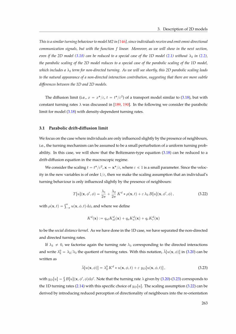
3. Description of 2D models
This is a similar turning behaviour tomodelM2 in [146], since individuals receive and emit omni-directional
communication signals, but with the function f linear. Moreover, as we will show in the next section,
even if the 2D model (3.18) can be reduced to a special case of the 1D model (2.1) without λ2 in (2.2),
the parabolic scaling of the 2D model reduces to a special case of the parabolic scaling of the 1D model,
which includes a λ2 term for non-directed turning. As we will see shortly, this 2D parabolic scaling leads
to the natural appearance of a non-directed interaction contribution, suggesting that there are more subtle
differences between the 1D and 2D models.
The diffusion limit (i.e., x “ x˚ε, t “ t˚ε2) of a transport model similar to (3.18), but with
constant turning rates λ was discussed in [189, 190]. In the following we consider the parabolic
limit for model (3.18) with density-dependent turning rates.
3.1 Parabolic drift-diffusion limit
We focus on the casewhere individuals are only influenced slightly by the presence of neighbours,
i.e., the turning mechanism can be assumed to be a small perturbation of a uniform turning prob-
ability. In this case, we will show that the Boltzmann-type equation (3.18) can be reduced to a
drift-diffusion equation in the macroscopic regime.
We consider the scaling t “ t˚ε2, x “ x˚ε, where ε ! 1 is a small parameter. Since the veloc-
ity in the new variables is of order 1ε, then we make the scaling assumption that an individual’s
turning behaviour is only influenced slightly by the presence of neighbours:
T ruspx, φ1, φq “ λ1
2π `λ2
2π Kd ˚ ρpx, tq ` ε λ3Bruspx, φ1, φq , (3.22)
with ρpx, tq “şπ
´πupx, φ, tqdφ, and where we define
Kdpxq :“ qalKdalpxq ` qaKd
apxq ` qrKdr pxq
to be the social distance kernel. As we have done in the 1D case, we have separated the non-directed
and directed turning rates.
If λ3 ‰ 0, we factorise again the turning rate λ3 corresponding to the directed interactions
and write λ02 “ λ2λ3 the quotient of turning rates. With this notation, λrupx, φqs in (3.20) can be
written as
λrupx, φqs “ λ02K
d ˚ upx, φ, tq ` ε yDrupx, φ, tqs , (3.23)
with yDrus “ş
Bruspx, φ1, φqdφ1. Note that the turning rate λ given by (3.20)-(3.23) corresponds to
the 1D turning rates (2.14) with this specific choice of yDrus. The scaling assumption (3.22) can be
derived by introducing reduced perception of directionality of neighbours into the re-orientation
263
6. Self-organised animal aggregation
function ω and into the orientation kernelsKoj ,
gjpϑq “ λ02 ` εGjpϑq ,
Koalpθ, φq “
12π p1´ ε cos pφ´ θqq ,
Kor ps,x, φq “
12π p1` ε cos pφ´ ψqq ,
Koaps,x, φq “
12π p1´ ε cos pφ´ ψqq ,
where Gjpϑq, j “ r, a, al are signal response functions to be chosen according to the biological con-
text. Substituting these expressions into the re-orientation terms (3.19), we define λ1 “ ηal`ηr`ηa
and we obtain (3.22) with a precise expression for the social response function Brus.
If λ1 “ 0, we further have λ2 “ λ32π andşπ
´πGjpφ
1 ´ φ ´ Rpφ1 ´ θqqdφ “ 0, j “ r, a, al as
the probability to turn to any new angle is 1. In addition, we want the turning function Rpϑq to
be close to an unbiased turning mechanism. This can be expressed by taking Rpϑq “ εϑ, which
indeed corresponds to weak interaction between individuals, [167]. We obtain Brus “ Balrus `
Barus `Brruswith
Balruspφ1, φq “
12π qalGalpφ
1 ´ φqKdal ˚ ρpx, tq (3.24)
´λ0
22π qal
ż
R2Kdalpx´ sq
ż π
´π
cos`
φ1 ´ θ˘
ups, θ, tqdθ ds ,
Br,aruspφ1, φq “
12π qr,aGr,apφ
1 ´ φqKdr,a ˚ ρpx, tq (3.25)
˘λ0
22π qr,a
ż
R2Kdr,apx´ sq cos
`
φ1 ´ ψ˘
ρps, tqds .
Remark 3.3. Note that in 2D, λ02 is introduced as the relative strength of non-directed and directed turning
kernels. This is part of the scaling assumption in 2D, whereas in 1D, we introduced it as part of the model
(2.1)-(2.2) before rescaling. Note that λ02 “ 12π in Fetecau’s model where no distinction is made between
directed and non-directed turning.
Let us introduce
Kd˚px˚q “
1εKd
ˆ
x˚
ε
˙
, B˚px˚, φ1, φq “1
2πBˆ
x˚
ε, φ1, φ
˙
.
Simplifying the notation by dropping ˚, system (3.18) writes in the new variables as
ε2Btu` ε γ eφ ¨∇xu “1
2π`
λ1 ` λ2Kd ˚ ρ
˘
pρ´ 2πuq (3.26)
` ε λ3 2πż π
´π
Bpx, φ1, φqupx, φ1, tqdφ1
´ ε λ3 2π upx, φ, tqż π
´π
Bpx, φ, φ1qdφ1 .
Using a Hilbert expansion approach, u “ u0 ` εu1 ` ε2u2 ` ..., and defining the macroscopic
densities ρi “şπ
´πui dφ for i P N0, we obtain at leading oder a relaxation towards a uniform
264
3. Description of 2D models
angular distribution at each position:
u0px, φ, tq “ ρ0px, tqF pφq, (3.27)
F pφq “1
2π1φPp´π,πs.
Integrating (3.26) with respect to the direction of motion φ, we obtain the continuity equation
Btρ0 ` γ
ż π
´π
eφ ¨∇x u1dφ “ 0. (3.28)
Comparing orders of ε and using (3.27), we can derive an expression for u1 in terms of u0, ρ0, ρ1,
u1 “1
2πρ1 ´ γeφ ¨∇xu0
λ1 ` λ2Kd ˚ ρ0
`ρ0λ3
λ1 ` λ2Kd ˚ ρ0
ż π
´π
Brρ0spx, φ1, φq ´Brρ0spx, φ, φ1qdφ1.
Substituting into (3.28), we arrive at a macroscopic drift-diffusion equation of the form
Btρ0 “ ∇x . pDrρ0s∇xρ0 ´ ρ0krρ0sq ,
where the macroscopic diffusion coefficient Drρ0s “ γ2p2pλ1 ` λ2Kd ˚ ρ0qq and the social flux
krρ0s “λ3 γ
λ1 ` λ2Kd ˚ ρ0
ż π
´π
ż π
´π
peφ ´ eφ1qBrρ0spx, φ1, φqdφ1dφ (3.29)
are both described in terms of microscopic quantities. In the context of collective behaviour of
animal groups, we make two further assumptions:
(i) Individuals can process information in a similar manner for all three types of social interac-
tions:
Galpϑq “ Grpϑq “ Gapϑq “: Gpϑq @ϑ .
(ii) Individuals have symmetric perception, in otherwords, they can process information equally
well from left and right. Then the turning probability function ω is bisymmetric,
ωp´α,´βq “ ωpα, βq ,
which implies symmetry of the signal response function G.
Under these assumptions, the first term of the social response functions Bjrus in (3.24) and (3.25)
cancels when substituted into the social flux (3.29). The second term contains the factor λ02 which
cancels with λ3 in (3.29), leaving us with a factor of λ2 in the social flux. Using (3.27), we can
simplify the social flux even further and obtain the drift-diffusion equation
Btρ “ ∇x . pD0rρs∇xρq ´∇x . pρkrρsq , (3.30a)
D0rρs “γ2
2pλ1 ` λ2Kd ˚ ρq, (3.30b)
krρspx, tq “ λ2πγ
λ1 ` λ2Kd ˚ ρ
ˆ
qrKdr pxq
x|x| ´ qaK
dapxq
x|x|
˙
˚ ρ . (3.30c)
265
6. Self-organised animal aggregation
For notational convenience, we dropped the zero in ρ0. Note that this equation is similar to the
1D drift-diffusion equation (2.15) obtained via the parabolic limit for linear social interactions.
Remark 3.4. Integrating the 2D scaling assumption (3.22), we have
λpx, φ1q “ λ1 ` λ2Kd ˚ ρpx, tq ` ε λ3
ż
Bruspx, φ1, φqdφ ,
which is a particular case of the 1D scaling assumption (2.14). More precisely, the 2D turning rate λpx, φ1q
corresponds to (2.2) on the projected velocity set t0, πu, with a linear turning function fpzq “ z and with
the non-directed and directed communication mechanisms given by
yN rus “Kd ˚ ρpx, tq,
y˘Dru`, u´s “
Gp0q `Gpπq2 Kd ˚ ρpx, tq (3.31)
¯ λ02
ż
RqalK
dalpx´ sq
`
u`ps1, tq ´ u´ps1, tq
˘
ds1
¯ λ02
ż x1
´8
`
qrKdr px´ sq ´ qaKd
apx´ sq˘
ρps, tqds1
˘ λ02
ż 8
x1
`
qrKdr px´ sq ´ qaKd
apx´ sq˘
ρps, tqds1 ,
where x “ px1, 0q, ρpx, tq “ u`px1, tq ` u´px1, tq “ upx1, tq, and where we used assumptions (i) and
(ii). Hence, model (2.1)-(2.14) with communication mechanism (3.31) corresponds exactly to the 2D non-
local kinetic model (3.18)-(3.22)-(3.24)-(3.25). This means, for instance, that the macroscopic 2D model
(3.30) reduces to the heat equation for λ2 “ 0, which is not the case in the parabolic limit (2.15) of the
corresponding 1D hyperbolic model (2.1) with the turning rates given by (2.2). In fact, our 2D scaling
assumption gjpϑq “ λ02 ` εGjpϑq, j “ al, r, a, introduces the relative strength of directed and non-
directed turning kernels into the expression of the social response function Brus, which is responsible for
the appearance of a factor λ2 in the drift of the macroscopic 2D model (3.30).
Remark 3.5. For some particular choices of distance kernels, the limiting parabolic model (3.30) can be
reduced to well known equations. Let us assume, for example, that the distance kernels are constant on the
whole domain,
Kdj pxq “ 1, j “ al, a, r . (3.32)
This assumption corresponds to a setting in which individuals interact equally well with all other individuals
present in the entire domain. This is true locally for example if we have many individuals packed in little
space. Under assumption (3.32) together with λ1 “ 0, model (3.30) simplifies to
Btρ “C0
λ2∆ρ` C1 ∇ .
ˆ
ρ
ż
R2eψρpsqds
˙
,
where
eψ “s´ x|s´ x| ,
266
3. Description of 2D models
and C0, C1 are constants depending only on γ, qal, qa, qr and the total massş
ρdx. If qa “ qr, then the
attraction and repulsion forces cancel out (C1 “ 0) and we obtain the heat equation. Let us henceforth
assume qa ‰ qr. Furthermore, we can write the social flux as
krρs “ ∇W ˚ ρ , (3.33)
where the interaction potential W : R2 ÝÑ R is given by W pxq “ C1|x|. In fact, for the more general
distance kernels (3.21) the social flux can also be written in the form (3.33), with the interaction potential
W behaving like |x| close to zero and decaying exponentially fast as |x| ÝÑ 8 (e.g. Morse potentials).
Therefore, we recover the diffusive aggregation equation
Btρ “ ∆ρ`∇ . pρ p∇W ˚ ρqq , (3.34)
which models the behaviour of particles interacting through a pairwise potential while diffusing with Brow-
nian motion. This type of equation has received a lot of attention in recent years because of its ubiquity in
modelling aggregation processes, such as collective behaviour of animals [237, 240, 28, 114] and bacterial
chemotaxis [41] (see also the references therein). In fact, model (3.34) is part of the family of aggregation-
diffusion equations presented in Part I. Here, we have linear diffusionm “ 1 and a non-singular interaction
kernel with power k “ 1 (using the notation of Part I). This means (3.34) falls into the diffusion-dominated
regime discussed in Chapter 4, see Definition 3.1 in Chapter 1.
3.2 Grazing collision limit
In the following, we consider another type of scaling that leads to parabolic equations, by focusing
on the case where individuals turn only a small angle upon interactions with neighbours. This
is biologically realistic as, for example, many migratory birds follow favourable winds or mag-
netic fields [244] and social interactions with neighbours might not have a considerable impact on
directional changes of individuals. The so-called grazing collisions, i.e. collisions with small de-
viation, correspond to this assumption. In this case, we show that the Boltzmann-type equation
(3.18) can be reduced to a Fokker–Planck equation with non-local advective and diffusive terms
in the orientation space.
For simplicity, the 2D kinetic model (3.18) can be re-written as
Bu
Bt` γeφ∇xu “ ´Q
´rus `Q`ru, us
with
Q´rus “ Q´r rus `Q´a rus `Q
´alrus, Q`ru, us “ Q`r ru, us `Q
`a ru, us `Q
`alru, us ,
Q´j rus “ λjpx, φqu, Q`j ru, us “
ż π
´π
Tjpx, φ1, φqupx, φ1, tqdφ1 , for j “ r, al, a.
267
6. Self-organised animal aggregation
Let us focus for now only on the alignment interactions, the analysis of attraction and repulsion in-
teractions is similar. The grazing collision assumption suggests that we can rescale the probability
of re-orientation as follows:
ωεal`
φ´ φ1, φ´ θ˘
“1εgε
´φ´ φ1 ´ εRpφ´ θq
ε
¯
.
Here, the parameter ε is related to the small re-orientation angle following interactionswith neigh-
bours moving in direction θ. If we denote by εβ “ φ´ φ1 ´ εRpφ´ θq, then since ωε integrates to
1, we obtain:
1 “ż π
´π
ωεalpφ´ φ1, φ´ θqdφ1 “
ż π`φ´Rpφ´θq
´π`φ´Rpφ´θq
gεpβqdβ “
ż π
´π
gεpβqdβ ,
by periodicity of gε.
Generally, when an interaction kernel in the Boltzmann equation presents a singularity point,
the troubles are avoided by considering a weak formulation of the Boltzmann operator [173, 87].
Expanding Qalrus :“ ´Q´alrus `Q`alru, us, we obtain for all ψ P C8c pr´π, πsq,
ż π
´π
Qalrusψpφqdφ “ ηal
ż π
´π
ˆ
12πρpx, tq ´ upx, φ, tq
˙
ψpφqdφ
`
ż π
´π
ż π
´π
ż
R2λ3qalK
dalpx´ sqK
0alpθ, φqupx, φ, tqups, θ, tq¨
ż π
´π
ωεalpφ´ φ1 , φ´ θq
“
ψpφ1q ´ ψpφq‰
dφ1dsdθdφ . (3.36)
By substituting φ1 “ φ´ εβ´ εRpφ´θq into the ψpφ1q term in (3.36), and then expanding in Taylor
series about φwe obtain:ż π
´π
ωεalpφ´ φ1, φ´ θq
”
ψpφ1q ´ ψpφqı
dφ1 «
ż π
´π
gεpβq”
`
´ εβ ´ εRpφ´ θq˘Bψ
Bφ`ε2
2`
β `Rpφ´ θq˘2 B2ψ
Bφ2
ı
dβ .
Equation (3.36) can thus be approximated byż π
´π
Qalrusψpφqdφ “ ηal
ż π
´π
ˆ
12πρpx, tq ´ upx, φ, tq
˙
ψpφqdφ
´
ż π
´π
B
Bφ
”
upx, φ, tqCεalru, x, φsı
ψpφqdφ
`
ż π
´π
B2
Bφ2
”
upx, φ, tqDεalru, x, φs
ı
ψpφqdφ
with the definitions
Cεalru, x, φs :“ż π
´π
ż
R2λ3qalK
dalpx´ sqK
0alpθ, φqA
εalpφ´ θqups, θ, tqdθds,
Dεalru, x, φs :“
ż π
´π
ż
R2λ3qalK
dalpx´ sqK
0alpθ, φqB
εalpφ´ θqups, θ, tqdθds ,
268
3. Description of 2D models
where
Aεalpφ´ θq :“´ ε`
M1pεq `M0pεqRpφ´ θq˘
,
Bεalpφ´ θq :“ε2
2`
M2pεq ` 2M1pεqRpφ´ θq `M0pεqRpφ´ θq2˘ ,
andMnpεq :“şπ
´πβngεpβq dβ, n “ 0, 1, 2, denote the moment generating functions of gεpβq. In a
similar manner we can approximate the attractive and repulsive non-local terms:ż π
´π
Qr,arusψpφqdφ “ ηr,a
ż π
´π
ˆ
12πρpx, tq ´ upx, φ, tq
˙
ψpφqdφ
´
ż π
´π
B
Bφ
´
upx, φ, tqCεr,aru, x, φs¯
ψpφqdφ
`
ż π
´π
B2
Bφ2
´
upx, φ, tqDεr,aru, x, φs
¯
ψpφqdφ ,
where
Cεr,aru, x, φs “
ż π
´π
ż
R2λ3qr,aK
dr,apx´ sqK
0r,aps, x, φqA
εr,aps, x, φqups, θ, tqdsdθ ,
Dεr,aru, x, φs “
ż π
´π
ż
R2λ3qr,aK
dr,apx´ sqK
0r,aps, x, φqB
εr,aps, x, φqups, θ, tqdsdθ ,
Aεr,aps, x, φq “ ´ εpM1pεqM0pεqRpφ´ ψsqq,
Bεr,aps, x, φq “ε2
2
”
M2pεq ` 2M1pεqRpφ´ ψsq `M0pεqRpφ´ ψsq2ı
.
Therefore, the kinetic model (3.18) in the strong formulation can be approximated (when individ-
uals turn only by a small angle upon interactions with their neighbours) by the following Fokker–
Planck model that contains all three social interactions:
Bu
Bt` γeφ ¨∇xu “λ1
ˆ
12πρpx, tq ´ upx, φ, tq
˙
(3.37)
`B
Bφ
”
´ uCεru, x, φs `B
BφpuDεru, x, φsq
ı
,
with λ1 “ ηa ` ηal ` ηr, and
Cεru, x, φs “ Cεalru, x, φs ` Cεr ru, x, φs ` C
εaru, x, φs ,
Dεru, x, φs “ Dεalru, x, φs `D
εrru, x, φs `D
εaru, x, φs .
While non-local 2D Fokker–Planck models have been introduced in the past years in connection
with self-organised aggregations, themajority of thesemodels consider local diffusion [123, 12]. If
we neglect the ε2 terms (i.e., Bε « 0) and assume λ1 “ 0, equation (3.37) reduces to a Vlasov-type
flocking equation:Bu
Bt` γeφ ¨∇xu`
B
Bφ
”
uCεru, x, φsı
“ 0 .
These type of models have been previously derived from individual-based models (Vicsek or
Cucker–Smale models) with or without noise [123, 179, 87].
269
6. Self-organised animal aggregation
4 Asymptotic preserving methods for 1D models
The kind of diffusion asymptotics we employed in the previous sections have been numerically
investigated in [88] using so-called asymptotic preserving (AP) schemes. The AP methods, which
improve the scheme already proposed in [169], are a fully explicit variation of the methods in-
troduced in [201, 202]. They are a powerful tool to investigate how patterns are preserved in the
parabolic limit by providing numerical schemes for all intermediate models of a scaling process
given some scaling parameter ε ą 0, and naturally produce a suitable numerical method for the
limiting model as ε Ñ 0. Here, we apply these schemes only to the 1D models introduced in
Section 2, since the numerics become much more complex in two dimensions. Taking advan-
tage of our understanding of the limit process, we base our scheme on a splitting strategy with
a convective-like step involving the transport part of the operator and an explicitly solvable ODE
step containing stiff sources (see Section 4.2).
4.1 Odd and even parity
We consider the 1D kinetic model (2.1) written as an odd-even decomposition,$
’
&
’
%
Btr ` γBxj “ 0 ,
Btj ` γBxr “ ´2λ`rr, jspr ` jq ` 2λ´rr, jspr ´ jq ,
with the equilibrium part (macro part/even part) r and the non-equilibrium part (micro part/odd
part) j given by
rpx, tq “12`
u`px, tq ` u´px, tq˘
, jpx, tq “12`
u`px, tq ´ u´px, tq˘
.
Under scaling assumption (2.10) for (2.2), this model reads in the new variables x “ xε, t “ tε2
as follows:
εBtr ` γBxj “0
εBtj ` γBxr “ rλ3pf ry´s ´ f ry`sq
´1εj`
2λ1 ` 4ελ2f`
KN ˚ r˘
` ελ3pf ry`s ` f ry´sq
˘
,
where KN pxq “ 1εK
N p xε q. Rearranging the terms and dropping ”„“ for notational convenience,
we obtain for r and J :“ 1ε j:
$
’
’
’
’
’
&
’
’
’
’
’
%
Btr ` γBxJ “0
BtJ ` γBxr “1ε2 rλ3pf ry
´s ´ f ry`sq `
ˆ
1´ 1ε2
˙
γBxr
´1ε2 J
`
2λ1 ` 4ελ2f`
KN ˚ r˘
` ελ3pf ry`s ` f ry´sq
˘
.
(4.38)
270
4. Asymptotic preserving methods for 1D models
4.2 Operator splitting
We can now employ an operator splitting method on (4.38), separating the stiff source part, which
can be treated by an implicit Euler method, and the transport part, which we can solve by an
explicit method such as upwinding:
1. Stiff source part:
Btr “0,
BtJ “1ε2 rλ3pf ry
´s ´ f ry`sq `
ˆ
1´ 1ε2
˙
γBxr (4.39)
´1ε2 J
`
2λ1 ` 4 ε λ2f`
KN ˚ r˘
` ε λ3pf ry`s ` f ry´sq
˘
.
2. Transport part:
Btr ` γ BxJ “ 0, (4.40)
BtJ ` γ Bxr “ 0 .
It can easily be verified that, in the limit ε Ñ 0, we recover indeed the macroscopic model (2.11)
for u “ 2r.
4.3 Alternated upwind discretisation
In the following, we are interested in the numerical implementation of model (2.1) with the turn-
ing rates (2.2) depending on a non-linear turning function f without a non-directed density-
dependent turning term (i.e. λ2 “ 0). As shown in Section 2.1, in this case, the parabolic limit
yields the drift-diffusion equation (2.11)
Btu “ D0Bxxu´ S0Bx`
upf´rus ´ f`rusq˘
,
with D0 “ γ2p2λ1q and S0 “ λ3γp2λ1q. Note the shorthand f˘rus “ fpy˘Drusq. We propose
an alternated upwind discretisation with the even part r evaluated at full grid points xi “ i∆x,
and the odd part J evaluated at half grid points xi` 12“ pi ` 1
2 q∆x. First, we discretise the stiff
source part (4.39) using an implicit Euler discretisation and respecting the direction of the drift.
We obtain an explicit expression for J˚,
J˚i` 1
2“
ε2Jni` 1
2` γ ∆t
∆x`
ε2 ´ 1˘ `
rni`1 ´ rni
˘
ε2 ` 2λ1∆t` ελ3∆t pf`rrns ` f´rrnsqi` 12
`
λ3∆t´
pf´rrns ´ f`rrnsq`
i` 12rni ` pf
´rrns ´ f`rrnsq´
i` 12rni`1
¯
ε2 ` 2λ1∆t` ελ3∆t pf`rrns ` f´rrnsqi` 12
,
271
6. Self-organised animal aggregation
with r˚ “ rn. Here, rn and Jn are the numerical solutions of r and J at time tn “ n∆t. We use
the ˚-notation for half steps in time. Since J is evaluated at half grid point, the discretisation of
the transport part (4.40) can be chosen independently of the sign of the drift,
1∆t
`
rn`1i ´ r˚i
˘
`1
∆x
´
J˚i` 1
2´ J˚
i´ 12
¯
“ 0 ,1
∆t
´
Jn`1i` 1
2´ J˚
i` 12
¯
`1
∆x`
r˚i`1 ´ r˚i
˘
“ 0 .
Taking the limit ε Ñ 0 in the expression for J˚i` 1
2and substituting into the first equation of the
transport part, we obtain the following discretisation of the one-dimensional macroscopic model
(2.11):
un`1i ´ uni
∆t “D0
p∆xq2´
Bpcqxxun¯
i
´S0
∆x
´
uni`
f´rrns ´ f`rrns˘`
i` 12´ uni´1
`
f´rrns ´ f`rrns˘`
i´ 12
¯
´S0
∆x
´
uni`1`
f´rrns ´ f`rrns˘´
i` 12´ uni
`
f´rrns ´ f`rrns˘´
i´ 12
¯
.
Here, Bpcqxxun denotes the standard central difference discretisations. This illustrates how the choice
of discretisation for (4.39) directly induces a discretisation of model (2.11). We will now use this
scheme to investigate how some of the patterns observed in model (2.1)-(2.2) change as εÑ 0.
Remark 4.1. The stability restriction for the proposed AP scheme is less clear. We can expect that the time
steps size ∆t needs to be sufficiently small, with an upper stability bound depending on the space step size
∆x, the diffusion coefficient D0, and the social interaction kernels via the termsKN ˚ u and f˘rus.
4.4 Simulation results
In Section 2.2 we have seen that for model M4, the two Hopf bifurcations that occurred for the k4
and k5 modes have disappeared as ε Ñ 0. In this Section, we start with a rotating wave pattern
(i.e., travelling pulses) that arises at ε “ 1 through a Hopf bifurcation (i.e., for the same parameter
values as in Figure 6.4: qa “ 1.545, qr “ 2.779, λ1 “ 0.2, λ2 “ 0, λ3 “ 0.9, γ “ 0.1, A “ 2). Then,
we investigate numerically what happens with this pattern as εÑ 0. The initial conditions for the
simulations are random perturbations of maximum amplitude 0.2 of the spatially homogeneous
steady state u˚ “ A2 “ 1. We start with ε “ 1, and run the numerical simulations up to t “ 1000.
Then we decrease ε, and choose the new initial condition to be the final solution obtained with
the previous ε value.
Figure 6.6(a) shows the amplitude of the patterns obtainedwhen ε P r0, 1s, for the particular pa-
rameter values mentioned before. Since some of these amplitudes show time-oscillations between
different values, we graph their maximum andminimum values for each ε. As we decrease ε from
1.0 towards 0.64 (region III), the amplitude undergoes some very small temporal oscillations (see
272
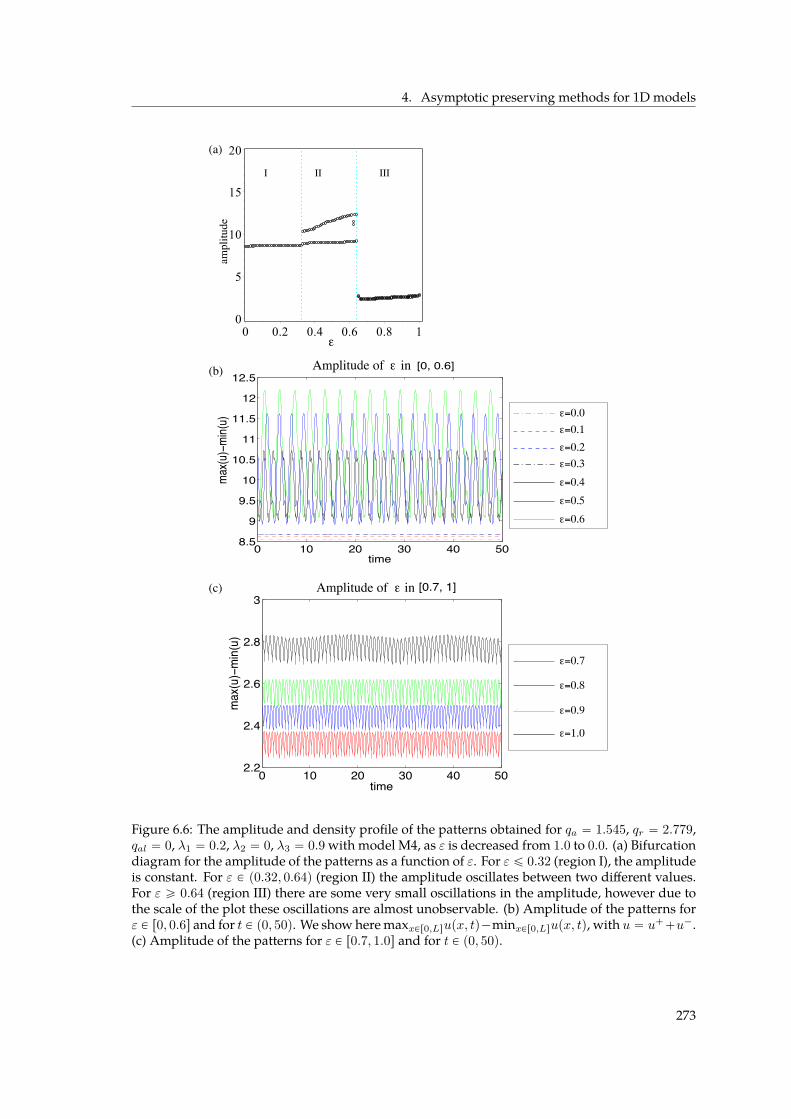
4. Asymptotic preserving methods for 1D models
0 10 20 30 40 508.5
9
9.5
10
10.5
11
11.5
12
12.5
time
A =
max(u
)−mi
n(u)
Amplitude for eps in [0, 0.6]
eps=0.6eps=0.5eps=0.4eps=0.3eps=0.2eps=0.1eps=0.0
0 10 20 30 40 502.2
2.4
2.6
2.8
3
time
A =
max
(u)−
min(
u)
Amplitude for eps in [0.7, 1]
eps=1.0
eps=0.9
eps=0.8
eps=0.7
¡
(b)
(c)
ampl
itude
IIIIII
(a)
¡=0.4
¡=0.5
¡=0.6
¡
¡Amplitude of in
Amplitude of in
¡=0.9
¡=0.7
¡=1.0
¡=0.1
¡=0.2
¡=0.8
¡=0.0
¡=0.3
Figure 6.6: The amplitude and density profile of the patterns obtained for qa “ 1.545, qr “ 2.779,qal “ 0, λ1 “ 0.2, λ2 “ 0, λ3 “ 0.9 with model M4, as ε is decreased from 1.0 to 0.0. (a) Bifurcationdiagram for the amplitude of the patterns as a function of ε. For ε ď 0.32 (region I), the amplitudeis constant. For ε P p0.32, 0.64q (region II) the amplitude oscillates between two different values.For ε ě 0.64 (region III) there are some very small oscillations in the amplitude, however due tothe scale of the plot these oscillations are almost unobservable. (b) Amplitude of the patterns forε P r0, 0.6s and for t P p0, 50q. We show heremaxxPr0,Lsupx, tq´minxPr0,Lsupx, tq, with u “ u``u´.(c) Amplitude of the patterns for ε P r0.7, 1.0s and for t P p0, 50q.
273
6. Self-organised animal aggregation
also panel (c)), corresponding to the rotatingwave patterns (with a small time-modulation) shown
in Figure 6.7(c). For ε P p0.32, 0.64q (region II), the amplitude oscillates between two large values.
This corresponds to the ”inside-group“ zigzagging behaviour shown in Figure 6.7(b) near x “ 6,
where the group as a whole does not move in space but individuals inside the group move be-
tween the left and right edges of the group. We also note a period-doubling bifurcation at ε “ 0.61
(region II, Figure 6.6(a); see the two dots that appear between the main branches), which leads to
a slight decrease in the amplitude. Finally, as ε is decreased below 0.32 (region I), the movement
inside the group is lost and the pattern is described by stationary pulses with fixed amplitude (see
Figure 6.6(a) and Figure 6.7(a)). Figures 6.6(b),(c) show the time-variation of the amplitudes of the
spatial and spatio-temporal patterns obtained for ε P r0, 1s. Figures 6.7(a’)-(c’) show the density
profiles of the patterns observed in regions I-III.
Because the macro-scale models (ε “ 0) seem to exhibit stationary pulses (as shown in Figure
6.7(a)), we now startwith these stationary pulses (for ε “ 1) and investigatewhether they change in
any way as εÑ 0. We focus here on model M2 (see Figure 6.3). Figure 6.8 shows the amplitude of
the stationary pulses obtainedwithmodelM2 in a particular parameter region (qa “ 2.2, qr “ 0.93,
qal “ 0; see also Figure 6.4), as we decrease the scaling parameter ε. We observe that in this case,
the scaling does not affect the patterns or their amplitudes.
Remark 4.2. Note that the rotating wave pattern shown in Figure 6.7(c) for ε “ 1 is obtained near a
Hopf/steady-state bifurcation (with k5 the Hopf wavenumber), and hence the 5 rotating peaks that form this
pattern. However, as εÑ 0, the wavenumber k3 seems to become unstable (hence the 3 peaks for the patterns
shown in Figure 6.7(a),(b)), even if the dispersion relation shown in Figure 6.4(b) suggests that k3 should
be stable.
5 Summary and discussion
In this chapter, we investigated the connections between a class of 1D and 2D non-local kinetic
models and their limit macroscopic models for self-organised biological aggregations. The non-
locality of thesemodels was the result of the assumptions that individuals can interact with neigh-
bours positioned further away, but still within their perception range. To simplify the kinetic mod-
els that incorporate microscopic-level interactions (such as individuals’ speed and turning rates),
we focused on two types of scalings, namely a parabolic and a grazing collision limit, which lead to
parabolic models described in terms of average speed and average turning behaviour. We showed
that while for the kinetic models the non-local interactions influence the turning rates (i.e., indi-
viduals turn to approach their neighbours, to move away from them or to align with them), for
the limit parabolic models the non-local interactions influence the dispersion and the drift of the
274
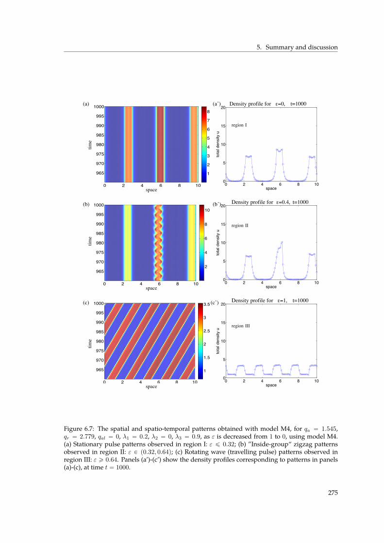
5. Summary and discussion
0 2 4 6 8 100
5
10
15
20
space
tota
l den
sity
u
Density profile for eps=0.4.t=1000
0 2 4 6 8 10
965
970
975
980
985
990
995
1000
1
1.5
2
2.5
3
3.5
0 2 4 6 8 10
965
970
975
980
985
990
995
1000
2
4
6
8
10
0 2 4 6 8 10
965
970
975
980
985
990
995
1000
1
2
3
4
5
6
7
8
0 2 4 6 8 100
5
10
15
20
space
tota
l den
sity
u
Density profile for eps=0.t=1000
0 2 4 6 8 100
5
10
15
20
space
tota
l den
sity
u
Density profile for eps=1.t=1000
region I
III
space
space
time
time
space
time
region
(a) (a’)
(b’)(b)
(c’)(c)
region
II
Density profile for t=1000
Density profile for t=1000
¡=0,
¡=1,
Density profile for t=1000¡=0.4,
Figure 6.7: The spatial and spatio-temporal patterns obtained with model M4, for qa “ 1.545,qr “ 2.779, qal “ 0, λ1 “ 0.2, λ2 “ 0, λ3 “ 0.9, as ε is decreased from 1 to 0, using model M4.(a) Stationary pulse patterns observed in region I: ε ď 0.32; (b) ”Inside-group“ zigzag patternsobserved in region II: ε P p0.32, 0.64q; (c) Rotating wave (travelling pulse) patterns observed inregion III: ε ě 0.64. Panels (a’)-(c’) show the density profiles corresponding to patterns in panels(a)-(c), at time t “ 1000.
275
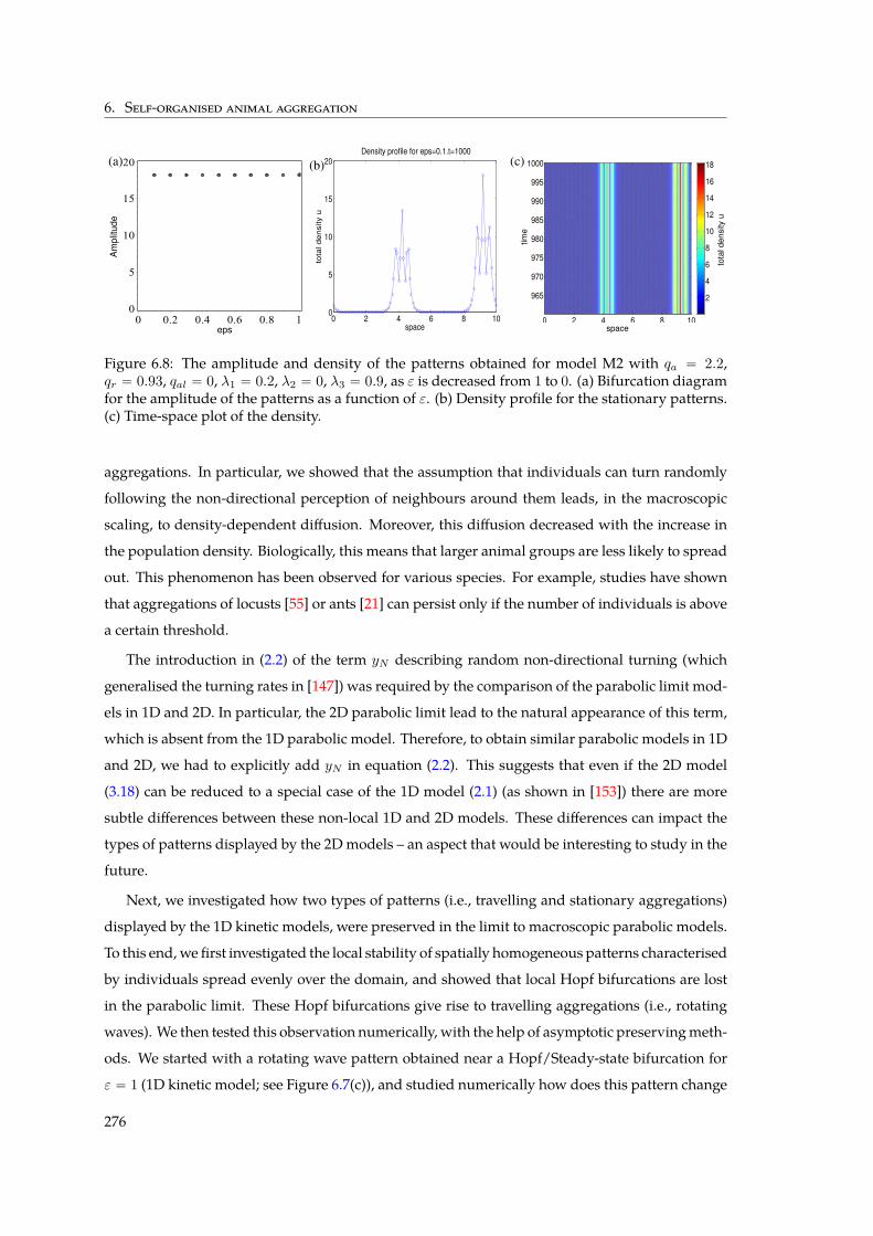
6. Self-organised animal aggregation
0 2 4 6 8 10
965
970
975
980
985
990
995
1000
2
4
6
8
10
12
14
16
18
0 2 4 6 8 100
5
10
15
20
space
tota
l density u
Density profile for eps=0.1.t=1000
tim
e
tota
l density u
Am
plit
ud
e
eps
(c)
space
(a) (b)
Figure 6.8: The amplitude and density of the patterns obtained for model M2 with qa “ 2.2,qr “ 0.93, qal “ 0, λ1 “ 0.2, λ2 “ 0, λ3 “ 0.9, as ε is decreased from 1 to 0. (a) Bifurcation diagramfor the amplitude of the patterns as a function of ε. (b) Density profile for the stationary patterns.(c) Time-space plot of the density.
aggregations. In particular, we showed that the assumption that individuals can turn randomly
following the non-directional perception of neighbours around them leads, in the macroscopic
scaling, to density-dependent diffusion. Moreover, this diffusion decreased with the increase in
the population density. Biologically, this means that larger animal groups are less likely to spread
out. This phenomenon has been observed for various species. For example, studies have shown
that aggregations of locusts [55] or ants [21] can persist only if the number of individuals is above
a certain threshold.
The introduction in (2.2) of the term yN describing random non-directional turning (which
generalised the turning rates in [147]) was required by the comparison of the parabolic limit mod-
els in 1D and 2D. In particular, the 2D parabolic limit lead to the natural appearance of this term,
which is absent from the 1D parabolic model. Therefore, to obtain similar parabolic models in 1D
and 2D, we had to explicitly add yN in equation (2.2). This suggests that even if the 2D model
(3.18) can be reduced to a special case of the 1D model (2.1) (as shown in [153]) there are more
subtle differences between these non-local 1D and 2D models. These differences can impact the
types of patterns displayed by the 2Dmodels – an aspect that would be interesting to study in the
future.
Next, we investigated how two types of patterns (i.e., travelling and stationary aggregations)
displayed by the 1D kinetic models, were preserved in the limit to macroscopic parabolic models.
To this end, we first investigated the local stability of spatially homogeneous patterns characterised
by individuals spread evenly over the domain, and showed that local Hopf bifurcations are lost
in the parabolic limit. These Hopf bifurcations give rise to travelling aggregations (i.e., rotating
waves). We then tested this observation numerically, with the help of asymptotic preservingmeth-
ods. We started with a rotating wave pattern obtained near a Hopf/Steady-state bifurcation for
ε “ 1 (1D kinetic model; see Figure 6.7(c)), and studied numerically how does this pattern change
276
5. Summary and discussion
when εÑ 0 (1D parabolic model; see Figure 6.7(a)). By graphing in Figure 6.6(a) the amplitude of
the resulting patterns as the scaling parameter ε is decreased from ε “ 1 to ε “ 0, we showed that
there were two major transitions. The first transition occurred around ε “ 0.64, when the travel-
ling (rotating) groups stopped moving. We note, however, that while the group as a whole was
stationary, the individuals inside the group were still moving between the left- and right-edges
of the group, leading to an ”inside-group“ zigzagging behaviour. The second transition occurred
around ε “ 0.32, when the individuals inside the groups stopped moving, leading to stationary
pulses.
We emphasise here that this study is one of the first in the literature to investigate numerically
the transitions between different aggregation patterns, as a scaling parameter ε is varied from val-
ues corresponding tomesoscale dynamics (ε “ 1) to values corresponding tomacroscale dynamics
(ε “ 0). Understanding these transitions is important when investigating biological phenomena
that occur on multiple scales, since it allows us to make decisions regarding the models that are
most suitable to reproduce the observed dynamics.
In this study we investigated the preservation of patterns via the 1D parabolic limit, but sim-
ilar investigations could be performed for the grazing collision limit. Moreover, as shown previ-
ously [146], model (2.1) can display many more types of complex spatio-temporal patterns than
the two types of patterns investigated here. We focused on travelling and stationary aggregations
since our aim here was not to investigate how all possible patterns are preserved by all these dif-
ferent scaling approaches. Rather, it was to show that by taking these asymptotic limits, some
patterns could be lost. Therefore, even if the macroscopic models are simpler to investigate, they
might not exhibit the same patterns as the kinetic models. Our analysis aimed at highlighting the
usefulness of asymptotic preserving numerical methods to understand the bifurcation of the so-
lutions as one investigates the transition from mesoscopic-level to macroscopic-level aggregation
dynamics.
277

Conclusions and Perspectives
Adding to the conclusions drawn in each of the previous chapters, let me comment on the main
goals, challenges and results of this thesis, as well as interesting questions and perspectives mov-
ing forward.
When tackling the question of long-time asymptotics in Parts I and II, the main challenges we
encounter are structural, and the main goal of this thesis is to develop new methods and analyt-
ical tools that allow to overcome these challenges. The motivation of our approach is not only to
tackle the models considered here, but to derive ideas that can then be applied to different prob-
lems with similar structural challenges.
More precisely, in Part I, the main structural challenge is the interplay between non-linear diffu-
sion and non-local interaction creating a rich set of possible behaviour of solutions. The main goal
is to obtain a complete characterisation for the asymptotic behaviour of solutions in all possible
parameter regimes. This thesis represents a step towards that goal. However, here, we mainly
focus on the fair-competition regime and make some investigations in the diffusion-dominated
regime. In short, for the fair-competition regime, we see that the behaviour of solutions is very
different depending on the sign of k. If k ă 0 (hencem ą 1) we observe a dichotomy similar to the
critical mass phenomenon of the classical Keller-Segel model, whereas for k ą 0 (hencem ă 1), no
such criticality exists. For both the fair-competition regime and the diffusion-dominated regime,
this family of models has not been analysed for the case of smooth potentials k ą 0 despite the
fact that there are interesting applications for this class of potentials.
To obtain the results presented in Part I, we made use of the special gradient flow structure of the
equation, as well as related functional inequalities by making the connection between stationary
states of the equation and global minimisers of the associated free energy functional. Further, in
one dimension, we used tools from optimal transportation to derive suitable functional inequali-
ties and obtain formally convergence to equilibrium in Wasserstein-2 distance.
279
Conclusions and Perspectives
Moving forward, I would like to contribute to a more general understanding of the behaviour
of solutions for this class of models, and the methods and tools developed in this thesis are the
necessary ground work to do that. In particular, the natural candidates amongst which to look
for asymptotic profiles are the equilibrium states of the system, and the first logical step towards
understanding the asymptotic behaviour of solutions is therefore to study the stationary problem
instead, which is our focus in Chapters 2, 3 and 4. Thanks to the analysis of the stationary problem
for the fair-competition regime and certain cases of the diffusion-dominated regime presented in
Part I, we are now able to advance a more rigorous analysis of the dynamical problem including
the time evolution of solutions.
Moreover, looking at the results we obtain, the question of the convexity properties of the energy
functionals Fk and Fk,resc arises. In fact, our analysis indicates that the behaviour of Fk or Fk,rescis that of convex functionals in certain regimes in the sense that existence of a global minimiser
implies its uniqueness (here only proven in one dimension). However, the overall convexity prop-
erties of Fk and Fk,resc are not known and there is certainly a bigger picture to be understood
there.
Finally, another important direction of future research is of course to investigate the parameter
regimes not considered in this thesis, such as the diffusion-dominated regime for k ą 0 and the
aggregation-dominated regime.
Part II is concernedwith a different application and a different equation, however, the question
we seek to answer is the same: What is the asymptotic behaviour of solutions? Themain goal is the
development of a suitable method to show convergence to equilibrium for certain types of kinetic
equationswhere the equilibrium state is not known a priori. We develop such amethod in the con-
text of a specific industrial application: modelling part of the production process of non-woven
textiles. In the case of a stationary conveyor belt κ “ 0, a hypocoercivity strategy has recently
been applied successfully to this kinetic fibre lay-down model to show exponential convergence
to equilibrium. In this case, the equilibrium distribution is known explicitly and the collision and
transport parts of the operator satisfy the necessary assumptions in an L2-framework. Adding the
movement of the belt however, we encounter two new structural challenges. First of all, we do not
know the equilibriumdistribution a priori which is usually the casewhen applying a hypocoerciv-
ity method. Secondly, as the perturbation of the moving belt only acts in one direction, it breaks
the symmetry of the problem. As a result, even if the existence of an equilibrium Fκ, κ ą 0, could
be guaranteed a priori, the collision and transport parts of the operator would not satisfy the good
assumptions in L2pF´1κ dxdαq, and so the standard hypocoercivity strategy cannot be applied.
The good news however is that hypocoercivity as a method is based on a priori estimates and is
therefore stable under perturbation. Our approach here is therefore to treat the system as a small
280
Conclusions and Perspectives
perturbation of the case κ “ 0. In order to control the perturbative term, we introduce not one,
but twomodifications of the ’natural’ entropy: 1) we first modify the space itself with a well-chosen
coercivity weight, then 2) we change the norm with an auxiliary operator following the standard
hypocoercivity approach, recovering the missing decay in the space variable. Further, in order to
overcome the structural difficulty of the hypocoercivity theory when the equilibrium distribution
is not known a priori, we derive a stronger hypocoercivity estimate for the generalised entropy
dissipation which holds on any solution and involving an additional mass term, instead of an
estimate on fluctuations around the equilibrium only. This hypocoercivity estimate is the key in-
gredient from which existence and uniqueness of a stationary state can be derived. Applied to
the difference between this stationary state and a solution of the same mass, it allows to deduce
exponential decay to equilibrium with an explicit rate.
There are several ways in which one could seek to improve the results in Part II. For example, one
could try to push the convergence result to larger values of κ using bifurcation techniques. More
precisely, for a path p : κ ÞÑ Fk mapping κ to the unique stationary state Fκ, our results in Part
II ensure that p is defined on a small interval r0, κ0q for some 0 ă κ0 ! 1. It may be possible to
extend this interval by showing that the implicit equation P pκ, Fκq “ 0 defining the stationary
state Fκ is non-degenerate, i.e. that B2P pκ, Fκq ‰ 0.
Another future avenue would be to apply the techniques developed here to other models where
the global equilibrium is not known a priori.
Finally, Part III is centred around the idea of understanding the relationship between different
kinetic andmacroscopicmodels for collective animal behaviour usingmultiscale analysis. Animal
groups are able to form beautiful patterns in the absence of a leader. We want to understand how
these patterns arrise and which are the driving factors behind the dynamics. In particular, the
goal of Part III is to understand how the different patterns are affected by the choice of modelling
scale. Understanding the transitions is important when investigating biological phenomena that
occur on multiple scales since it allows us to make decisions regarding the choice of models that
are most suitable to reproduce the observed dynamics. To achieve this, we use both analytical and
numerical tools.
Firstly, we develop a common framework for a class of collective animal behaviourmodels, making
the connection between non-local kinetic 1D and 2Dmodels with the corresponding macroscopic
models via parabolic and grazing collision limits. We observe that if we allow individuals to turn
randomly following the non-directional perception of neighbours produces a density-dependent
diffusion in the 1D and 2D parabolic limit. This diffusion decreases with increasing population
density, a phenomenon which makes biological sense since larger groups are less likely to spread
out. Taking a grazing collision limit in 2D, we obtain a Fokker-Planck equation with non-local
281
Conclusions and Perspectives
advective and diffusive terms in orientation space, whereas the majority of non-local 2D Fokker-
Planck models concerned with self-organised aggregations consider local diffusion only. A fur-
ther simplification of the limiting equation reduces it to a Vlasov-type flocking equation, a class
of models that have previously been derived from individual-based models directly (Vicsek or
Cucker–Smale models). The analysis of this limiting equation would be another interesting av-
enue for further research.
Secondly, we investigate how some of the kinetic spatio-temporal patterns are preserved via these
scalings using asymptotic preserving numerical methods. We observe that certain patterns such
as stationary aggregations are preserved, while others, e.g. moving aggregations, are lost. There-
fore, even if the macroscopic models are simpler to investigate, they might not exhibit the same
patterns as the kinetic models. This is an important information for choosing a modelling scale
that is well adapted to the dynamics one would like to capture. It also serves to demonstrate the
usefulness of AP schemes in understanding the bifurcation of solutions as εÑ 0 as they are able
to simulate themodels on all the intermediate scales as well using one single scheme. AP schemes
have only recently been applied to investigate multiscale aspects of biological aggregations and
they provide a useful tool for further analysis of pattern formations on different scales.
The process of writing this thesis made me realise that what I am interested in are research
questions leading to the development of newmethods and tools and that allow for a better under-
standing of the bigger picture around a certain problem. It is exciting howmathematical ideas can
draw connections between very different subject areas and can therefore contribute to advances
across disciplines.
282
Bibliography
[1] R. Alonso, T. Goudon, and A. Vavasseur. Damping of particles interacting with a vibrating
medium. Annales de l’Institut Henri Poincare (C) Non Linear Analysis, 2017.
[2] W. Alt. Biased random walk models for chemotaxis and related diffusion approximations.
J. Math. Biol., 9(2):147–177, 1980.
[3] L. A. Ambrosio, N. Gigli, and G. Savaré. Gradient flows in metric spaces and in the space of
probability measures. Lectures in Mathematics. Birkhäuser, 2005.
[4] G. E. Andrews, R. Askey, and R. Roy. Special functions, volume 71 of Encyclopedia of Mathe-
matics and its Applications. Cambridge University Press, Cambridge, 1999.
[5] E. D. Angelis and B. Lods. On the kinetic theory for active particles: a model for tumor-
immune system competition. Mathematical and Computer Modeling, 47:196–209, 2008.
[6] A. Arnold, J. A. Carrillo, I. Gamba, and C.-w. Shu. Low and high field scaling limits for the
vlasov- and wigner-poisson-fokker-planck systems. Transp. Theory Stat. Phys., 30:121–153,
2001.
[7] D. G. Aronson. The porous medium equation. In Nonlinear diffusion problems (Montecatini
Terme, 1985), volume 1224 of Lecture Notes in Math., pages 1–46. Springer, Berlin, 1986.
[8] A. A. Arsen’ev and O. E. Buryak. On a connection between the solution of the Boltzmann
equation and the solution of the Landau-Fokker-Planck equation. Mat. Sb., 181(4):435–446,
1990.
[9] D. Bakry and M. Émery. Diffusions hypercontractives. In Séminaire de probabilités, XIX,
1983/84, volume 1123 of Lecture Notes in Math., pages 177–206. Springer, Berlin, 1985.
[10] D. Balagué, J. A. Carrillo, T. Laurent, and G. Raoul. Dimensionality of local minimizers of
the interaction energy. Arch. Ration. Mech. Anal., 209(3):1055–1088, 2013.
283
Bibliography
[11] D. Balagué, J. A. Carrillo, T. Laurent, and G. Raoul. Nonlocal interactions by repulsive-
attractive potentials: radial ins/stability. Phys. D, 260:5–25, 2013.
[12] A. Barbaro and P. Degond. Phase transition and diffusion among socially interacting self-
propelled agents. Discrete Cont Dyn Syst B. In Press, 2013.
[13] C. Bardos, R. Santos, and R. Sentis. Diffusion approximation and computation of the critical
size. Trans. Amer. Math. Soc., 284(2):617–649, 1984.
[14] G. I. Barenblatt. On some unsteady motions of a liquid and gas in a porous medium. Akad.
Nauk SSSR. Prikl. Mat. Meh., 16:67–78, 1952.
[15] G. I. Barenblatt. Scaling, self-similarity, and intermediate asymptotics, volume 14 of Cambridge
Texts inAppliedMathematics. CambridgeUniversity Press, Cambridge, 1996. With a foreword
by Ya. B. Zeldovich.
[16] G. I. Barenblatt and P. Makinen. Dimensional Analysis. Gordon & Breach Publishing Group,
1987.
[17] F. Barthe. Inégalités de Brascamp-Lieb et convexité. C. R. Math. Acad. Sci. Paris, 324:885–888,
1997.
[18] F. Barthe. On a reverse form of the Brascamp-Lieb inequality. Invent. Math., 310:685–693,
1998.
[19] W. Beckner. Sharp Sobolev inequalities on the sphere and the Moser-Trudinger inequality.
Ann. of Math., 138:213–242, 1993.
[20] J. Bedrossian, N. Rodríguez, and A. L. Bertozzi. Local and global well-posedness for aggre-
gation equations and Patlak-Keller-Segel models with degenerate diffusion. Nonlinearity,
24(6):1683–1714, 2011.
[21] M. Beekman, D. J. T. Sumpter, and F. L. W. Ratnieks. Phase transitions between disordered
and ordered foraging in pharaoh’s ants. Proc. Natl. Acad. Sci., 98(17):9703–9706, 2001.
[22] N. Bellomo, E. D. Angelis, and L. Preziosi. Multiscalemodeling andmathematical problems
related to tumor evolution andmedical therapy. Journal of Theoretical Medicine, 5(2):111–136,
2003.
[23] N. Bellomo, A. Bellouquid, J. Nieto, and J.Soler. Multicellular biological growing systems:
hyperbolic limits towards macroscopic description. Mathematical Models and Methods in Ap-
plied Sciences, 17:1675–1693, 2007.
284
[24] N. Bellomo, C. Bianca, andM.Delitala. Complexity analysis andmathematical tools towards
the modelling of living systems. Physics of Life Reviews, 6:144–175, 2009.
[25] P. Bénilan andM.G. Crandall. The continuous dependence onϕ of solutions of ut´∆ϕpuq “
0. Indiana Univ. Math. J., 30(2):161–177, 1981.
[26] A. Bensoussan, J.-L. Lions, and G. C. Papanicolaou. Boundary layers and homogenization
of transport processes. Publications of the Research Institute for Mathematical Sciences, 15(1):53–
157, 1979.
[27] M. G. Bertotti and M. Delitala. Conservation laws and asymptotic behavior of a model of
social dynamics. Nonlinear Analysis RWA, 9:183–196, 2008.
[28] A. L. Bertozzi, J. A. Carrillo, and T. Laurent. Blow-up in multidimensional aggregation
equations with mildly singular interaction kernels. Nonlinearity, 22(3):683–710, 2009.
[29] A. L. Bertozzi, T. Kolokolnikov, H. Sun, D. Uminsky, and J. von Brecht. Ring patterns and
their bifurcations in a nonlocal model of biological swarms. Commun. Math. Sci., 13(4):955–
985, 2015.
[30] A. L. Bertozzi and T. Laurent. Finite-time blow-up of solutions of an aggregation equation
in Rn. Comm. Math. Phys., 274(3):717–735, 2007.
[31] A. L. Bertozzi, T. Laurent, and J. Rosado. Lp theory for the multidimensional aggregation
equation. Comm. Pure Appl. Math., 64(1):45–83, 2011.
[32] S. Bian and J.-G. Liu. Dynamic and steady states for multi-dimensional Keller-Segel model
with diffusion exponentm ą 0. Comm. Math. Phys., 323(3):1017–1070, 2013.
[33] P. Biler, G. Karch, P. Laurençot, and T. Nadzieja. The 8π-problem for radially symmetric
solutions of a chemotaxis model in the plane. Math. Methods Appl. Sci., 29(13):1563–1583,
2006.
[34] P. Biler and T. Nadzieja. Existence and nonexistence of solutions for a model of gravitational
interaction of particles. Colloq. Math., 66:319–334, 1994.
[35] A. Blanchet, M. Bonforte, J. Dolbeault, G. Grillo, and J.-L. Vázquez. Asymptotics of the fast
diffusion equation via entropy estimates. Arch. Ration. Mech. Anal., 191(2):347–385, 2009.
[36] A. Blanchet, V. Calvez, and J. A. Carrillo. Convergence of themass-transport steepest descent
scheme for the subcritical Patlak-Keller-Segel model. SIAM J. Numer. Anal., 46(2):691–721,
2008.
285
Bibliography
[37] A. Blanchet, E. A. Carlen, and J. A. Carrillo. Functional inequalities, thick tails and asymp-
totics for the critical mass Patlak-Keller-Segel model. J. Funct. Anal., 262(5):2142–2230, 2012.
[38] A. Blanchet and G. Carlier. From Nash to Cournot-Nash equilibria via the Monge-
Kantorovich problem. Philos. Trans. R. Soc. Lond. Ser. A Math. Phys. Eng. Sci.,
372(2028):20130398, 11, 2014.
[39] A. Blanchet, J. A. Carrillo, and P. Laurençot. Critical mass for a Patlak-Keller-Segel model
with degenerate diffusion in higher dimensions. Calc. Var. Partial Differential Equations,
35(2):133–168, 2009.
[40] A. Blanchet, J. A. Carrillo, andN.Masmoudi. Infinite time aggregation for the critical Patlak-
Keller-Segel model in R2. Comm. Pure Appl. Math., 61(10):1449–1481, 2008.
[41] A. Blanchet, J. Dolbeault, and B. Perthame. Two dimensional Keller-Segel model inR2: opti-
mal critical mass and qualitative properties of the solution. Electron. J. Differential Equations,
2006(44):1–33 (electronic), 2006.
[42] M. Bodnar and J. J. L. Velazquez. Derivation of macroscopic equations for individual cell-
based models: a formal approach. Math. Meth. Appl. Sci., 28:1757–1779, 2005.
[43] M. Bodnar and J. J. L. Velázquez. Friction dominated dynamics of interacting particles lo-
cally close to a crystallographic lattice. Math. Methods Appl. Sci., 36(10):1206–1228, 2013.
[44] F. Bolley, I. Gentil, and A. Guillin. Uniform convergence to equilibrium for granular media.
Arch. Ration. Mech. Anal., 208(2):429–445, 2013.
[45] L. Boltzmann. Lectures on gas theory. Translated by StephenG. Brush. University of California
Press, Berkeley-Los Angeles, Calif., 1964.
[46] L. Boltzmann. Weitere Studien über dasWärmegleichgewicht unter Gasmolekülen, pages 115–225.
Vieweg+Teubner Verlag, Wiesbaden, 1970.
[47] M. Bonforte, J. Dolbeault, G. Grillo, and J. L. Vázquez. Sharp rates of decay of solutions to
the nonlinear fast diffusion equation via functional inequalities. Proc. Natl. Acad. Sci. USA,
107(38):16459–16464, 2010.
[48] M. Bonforte and J. L. Vazquez. Global positivity estimates and Harnack inequalities for the
fast diffusion equation. J. Funct. Anal., 240(2):399–428, 2006.
[49] E. Bouin, F. Hoffmann, and C. Mouhot. Exponential decay to equilibrium for a fibre lay-
down process on a moving conveyor belt. Preprint arXiv:1605.04121v3.
286
[50] D. P. Bourne and S. M. Roper. Centroidal power diagrams, Lloyd’s algorithm, and applica-
tions to optimal location problems. SIAM J. Numer. Anal., 53(6):2545–2569, 2015.
[51] V. Boussinesq. Recherches théoriques sur l’écoulement des nappes d’eau infiltrées dans le sol et sur
le débit des sources, volume 10 of Comptes Rendus Acad. Sci. / Journal de mathématiques pures et
appliquées.
[52] R. Breitwisch and G. Whitesides. Directionality of singing and non-singing behaviour of
mated and unmated Northern Mockingbirds, Mimus polyglottos. Anim. Behav., 35:331–339,
1987.
[53] Y. Brenier. Polar factorization and monotone rearrangement of vector-valued functions.
Comm. Pure Appl. Math., 44:375–417, 1991.
[54] F. Brock and A. Y. Solynin. An approach to symmetrization via polarization. Trans. Amer.
Math. Soc., 352(4):1759–1796, 2000.
[55] J. Buhl, D. J. T. Sumpter, I. D. Couzin, J. J. Hale, E. Despland, E. R. Miller, and S. J. Simpson.
From disorder to order in marching locusts. Science, 312:1402–1406, 2006.
[56] P.-L. Buono and R. Eftimie. Analysis of Hopf/Hopf bifurcations in nonlocal hyperbolic
models for self-organised aggregations. Math. Models Methods Appl. Sci., 24:327, 2014.
[57] P.-L. Buono and R. Eftimie. Codimension-two bifurcations in animal aggregation models
with symmetry. SIAM J. Appl. Dyn. Syst., 2014.
[58] P.-L. Buono and R. Eftimie. Symmetries and pattern formation in hyperbolic versus
parabolic models for self-organised aggregations. J. Math. Biol., 2014.
[59] M. Burger, V. Capasso, and D. Morale. On an aggregation model with long and short range
interactions. Nonlinear Analysis: Real World Applications, 8:939–958, 2007.
[60] L. A. Caffarelli and P. R. Stinga. Fractional elliptic equations, Caccioppoli estimates and
regularity. Ann. Inst. H. Poincaré Anal. Non Linéaire, 33(3):767–807, 2016.
[61] V. Calvez and J. A. Carrillo. Volume effects in the Keller-Segel model: energy estimates
preventing blow-up. J. Math. Pures Appl., 86:155–175, 2006.
[62] V. Calvez and J. A. Carrillo. Refined asymptotics for the subcritical Keller-Segel system and
related functional inequalities. Proc. Amer. Math. Soc., 140(10):3515–3530, 2012.
[63] V. Calvez, J. A. Carrillo, and F. Hoffmann. Equilibria of homogeneous functionals in the
fair-competition regime. Nonlinear Anal., 159:85–128, 2017.
287
Bibliography
[64] V. Calvez, J. A. Carrillo, and F. Hoffmann. The geometry of diffusing and self-attracting
particles in a one-dimensional fair-competition regime. In Nonlocal and Nonlinear Diffusions
and Interactions: New Methods and Directions, volume 2186 of Lecture Notes in Math. Springer,
[Cham], 2017.
[65] V. Calvez and L. Corrias. Blow-up dynamics of self-attracting diffusive particles driven by
competing convexities. Discrete Contin. Dyn. Syst. Ser. B, 18(8):2029–2050, 2013.
[66] V. Calvez and T. O. Gallouët. Blow-up phenomena for gradient flows of discrete homoge-
neous functionals. Preprint arXiv:1603.05380v2.
[67] V. Calvez and T. O. Gallouët. Particle approximation of the one dimensional Keller-Segel
equation, stability and rigidity of the blow-up. Discrete Contin. Dyn. Syst., 36(3):1175–1208,
2016.
[68] V. Calvez, B. Perthame, andM. Sharifi tabar. Modified Keller-Segel system and critical mass
for the log interaction kernel. In Stochastic analysis and partial differential equations, volume
429 of Contemp. Math., pages 45–62. Amer. Math. Soc., Providence, RI, 2007.
[69] V. Calvez, G. Raoul, and C. Schmeiser. Confinement by biased velocity jumps: aggregation
of Escherichia coli. Kinet. Relat. Models, 8(4):651–666, 2015.
[70] J. F. Campos and J. Dolbeault. A functional framework for the Keller-Segel system: logarith-
mic Hardy-Littlewood-Sobolev and related spectral gap inequalities. C. R. Math. Acad. Sci.
Paris, 350(21-22):949–954, 2012.
[71] J. F. Campos and J. Dolbeault. Asymptotic estimates for the parabolic-elliptic Keller-Segel
model in the plane. Comm. Partial Differential Equations, 39(5):806–841, 2014.
[72] J. A. Cañizo, J. A. Carrillo, and F. S. Patacchini. Existence of compactly supported global
minimisers for the interaction energy. Arch. Ration. Mech. Anal., 217(3):1197–1217, 2015.
[73] E. A. Carlen. Duality and stability for functional inequalities. Preprint arXiv:1609.00936.
[74] E. A. Carlen, J. A. Carrillo, and M. Loss. Hardy-Littlewood-Sobolev inequalities via fast
diffusion flows. Proc. Natl. Acad. Sci. USA, 107(46):19696–19701, 2010.
[75] E. A. Carlen and A. Figalli. Stability for a GNS inequality and the log-HLS inequality, with
application to the critical mass Keller-Segel equation. Duke Math. J., 162(3):579–625, 2013.
[76] E. A. Carlen, R. L. Frank, and E. H. Lieb. Stability estimates for the lowest eigenvalue of a
Schrödinger operator. Geom. Funct. Anal., 24(1):63–84, 2014.
288
[77] E. A. Carlen and M. Loss. Competing symmetries, the logarithmic HLS inequality and
Onofri’s inequality on Sn. Geom. Funct. Anal., 2:90–104, 1992.
[78] J. A. Carrillo, D. Castorina, and B. Volzone. Ground states for diffusion dominated free
energies with logarithmic interaction. SIAM J. Math. Anal., 47(1):1–25, 2015.
[79] J. A. Carrillo, M. Chipot, and Y. Huang. On global minimizers of repulsive-attractive
power-law interaction energies. Philos. Trans. R. Soc. Lond. Ser. A Math. Phys. Eng. Sci.,
372(2028):20130399, 13, 2014.
[80] J. A. Carrillo, Y.-P. Choi, and M. Hauray. The derivation of swarming models: mean-field
limit and Wasserstein distances. In Collective dynamics from bacteria to crowds, volume 553 of
CISM Courses and Lect., pages 1–46. Springer, Vienna, 2014.
[81] J. A. Carrillo, M. G. Delgadino, and A. Mellet. Regularity of local minimizers of the interac-
tion energy via obstacle problems. To appear in Comm. Math. Phys., preprint arXiv:1406.4040
[math.AP], 2014.
[82] J. A. Carrillo, M. DiFrancesco, A. Figalli, T. Laurent, and D. Slepcev. Global-in-time weak
measure solutions and finite-time aggregation for nonlocal interaction equations. Duke
Math. J., 156(2):229–271, 2011.
[83] J. A. Carrillo, M. R. D’Orsogna, and V. Panferov. Double milling in self-propelled swarms
from kinetic theory. Kinetic and Related Models, 2:363–378, 2009.
[84] J. A. Carrillo, R. Eftimie, and F. Hoffmann. Non-local kinetic and macroscopic models for
self-organised animal aggregations. Kinet. Relat. Models, 8(3):413–441, 2015.
[85] J. A. Carrillo, L. C. F. Ferreira, and J. C. Precioso. A mass-transportation approach to a one
dimensional fluidmechanicsmodelwith nonlocal velocity. Adv.Math., 231(1):306–327, 2012.
[86] J. A. Carrillo, M. Fornasier, J. Rosado, and G. Toscani. Asymptotic flocking dynamics for the
kinetic Cucker-Smale model. SIAM J. Math. Anal., 42:218–236, 2010.
[87] J. A. Carrillo, M. Fornasier, G. Toscani, and F. Vecil. Particle, kinetic, and hydrodynamic
models of swarming. In Mathematical modeling of collective behavior in socio-economic and life
sciences, Model. Simul. Sci. Eng. Technol., pages 297–336. Birkhäuser Boston, Inc., Boston,
MA, 2010.
[88] J. A. Carrillo, T. Goudon, P. Lafitte, and F. Vecil. Numerical schemes of diffusion asymptotics
and moment closures for kinetic equations. J. Sci. Comput., 36(1):113–149, 2008.
289
Bibliography
[89] J. A. Carrillo, S. Hittmeir, B. Volzone, andY. Yao. Nonlinear aggregation-diffusion equations:
Radial symmetry and long time asymptotics. Preprint arXiv:1603.07767.
[90] J. A. Carrillo, F. Hoffmann, E. Mainini, and B. Volzone. Ground states in the diffusion-
dominated regime. Preprint arXiv:1705.03519.
[91] J. A. Carrillo, Y. Huang, and S. Martin. Explicit flock solutions for Quasi-Morse potentials.
European J. Appl. Math., 25(5):553–578, 2014.
[92] J. A. Carrillo, A. Jüngel, P. A.Markowich, G. Toscani, andA. Unterreiter. Entropy dissipation
methods for degenerate parabolic problems and generalized Sobolev inequalities. Monatsh.
Math., 133(1):1–82, 2001.
[93] J. A. Carrillo, A. Klar, S. Martin, and S. Tiwari. Self-propelled interacting particle systems
with roosting force. Math. Models Methods Appl. Sci., 20:1533, 2010.
[94] J. A. Carrillo, S. Lisini, and E.Mainini. Uniqueness for Keller-Segel-type chemotaxis models.
Discrete Contin. Dyn. Syst., 34(4):1319–1338, 2014.
[95] J. A. Carrillo, S. Martin, and V. Panferov. A new interaction potential for swarming models.
Phys. D, 260:112–126, 2013.
[96] J. A. Carrillo, R. J. McCann, and C. Villani. Kinetic equilibration rates for granular media
and related equations: entropy dissipation and mass transportation estimates. Rev. Mat.
Iberoamericana, 19:1–48, 2003.
[97] J. A. Carrillo, R. J. McCann, and C. Villani. Contractions in the 2-Wasserstein length space
and thermalization of granular media. Arch. Ration. Mech. Anal., 179:217–263, 2006.
[98] J. A. Carrillo and D. Slepcev. Example of a displacement convex functional of first order.
Calc. Var. Partial Differential Equations, 36(4):547–564, 2009.
[99] J. A. Carrillo and Y. Sugiyama. Compactly supported stationary states of the degenerate
keller-segel system in the diffusion-dominated regime. Preprint arXiv:1612.05375.
[100] J. A. Carrillo and G. Toscani. Asymptotic L1-decay of solutions of the porous medium equa-
tion to self-similarity. Indiana Univ. Math. J., 49(1):113–142, 2000.
[101] J. A. Carrillo and J. L. Vázquez. Fine asymptotics for fast diffusion equations. Comm. Partial
Differential Equations, 28(5-6):1023–1056, 2003.
[102] J. A. Carrillo and B. Yan. An asymptotic preserving scheme for the diffusive limit of kinetic
systems for chemotaxis. Multiscale Model. Simul., 11(1):336–361, 2013.
290
[103] C. Cercignani, R. Illner, andM. Pulvirenti. The mathematical theory of dilute gases, volume 106
of Applied Mathematical Sciences. Springer-Verlag, New York, 1994.
[104] F. Chalub, P. Markowich, B. Perthame, and C. Schmeiser. Kinetic models for chemotaxis and
their drift-diffusion limits. Monatsh. Math., 142:123–141, 2004.
[105] S. Chandrasekhar. Principles of stellar dynamics. Enlarged ed. Dover Publications, Inc., New
York, 1960.
[106] P.-H. Chavanis, P. Laurençot, and M. Lemou. Chapman-Enskog derivation of the general-
ized Smoluchowski equation. Phys. A, 341(1-4):145–164, 2004.
[107] P. H. Chavanis and R. Mannella. Self-gravitating Brownian particles in two dimensions: the
case of N “ 2 particles. Eur. Phys. J. B, 78(2):139–165, 2010.
[108] P.-H. Chavanis and C. Sire. Anomalous diffusion and collapse of self-gravitating langevin
particles in d dimensions. Phys. Rev. E, 69:016116, Jan 2004.
[109] L. Chen, J.-G. Liu, and J. Wang. Multidimensional degenerate Keller-Segel system with
critical diffusion exponent 2npn` 2q. SIAM J. Math. Anal., 44(2):1077–1102, 2012.
[110] L. Chen and J.Wang. Exact criterion for global existence and blow up to a degenerate Keller-
Segel system. Doc. Math., 19:103–120, 2014.
[111] S. Chen, R. Frank, and T.Weth. Remainder terms in the fractional Sobolev inequality. Indiana
Univ. Math. J., 62:1381–1397, 2013.
[112] A. Chertock, A. Kurganov, A. Polizzi, and I. Timofeyev. Pedestrian flow models with slow-
down interactions. Math Models Methods Appl. Sci., 24(2):249–275, 2014.
[113] S. Childress and J. K. Percus. Nonlinear aspects of chemotaxis. Math. Biosciences, 56:217–237,
1981.
[114] Y.-L. Chuang, M. R. D’Orsogna, D. Marthaler, A. L. Bertozzi, and L. S. Chayes. State transi-
tions and the continuum limit for a 2d interactiong, self-propelled particle system. Physica
D, 232:33–47, 2007.
[115] T. Cieślak and P. Laurençot. Looking for critical nonlinearity in the one-dimensional quasi-
linear Smoluchowski-Poisson system. Discrete Contin. Dyn. Syst., 26(2):417–430, 2010.
[116] T. Cieślak and P. Laurençot. Global existence vs. blowup in a one-dimensional
Smoluchowski-Poisson system. In Parabolic problems, volume 80 of Progr. Nonlinear Differ-
ential Equations Appl., pages 95–109. Birkhäuser/Springer Basel AG, Basel, 2011.
291
Bibliography
[117] D. Cordero-Erausquin, B. Nazaret, and C. Villani. Amass-transportation approach to sharp
Sobolev and Gagliardo-Nirenberg inequalities. Adv. Math., 182(2):307–332, 2004.
[118] L. Corrias, B. Perthame, andH. Zaag. Global solutions of some chemotaxis and angiogenesis
systems in high space dimensions. Milan J. Math., 72:1–28, 2004.
[119] K. Craig. Nonconvex gradient flow in thewassersteinmetric and applications to constrained
nonlocal interactions. Preprint arXiv:1512.07255v1.
[120] P. Degond, G. Dimarco, and T. Mac. Hydrodynamics of the Kuramoto-Vicsek model of
rotating self-propelled particles.MathematicalModels andMethods in Applied Sciences, 24:277–
325, 2014.
[121] P. Degond, T. Goudon, and F. Poupaud. Diffusion limit for nonhomogeneous and non-
micro-reversible processes. Indiana Univ. Math. J., 49(3):1175–1198, 2000.
[122] P. Degond and B. Lucquin-Desreux. The Fokker-Planck asymptotics of the Boltzmann col-
lision operator in the Coulomb case. Math. Models Methods Appl. Sci., 2(2):167–182, 1992.
[123] P. Degond and S. Motsch. Macroscopic limit of self-driven particles with orientation inter-
action. C.R. Acad. Sci. Paris Ser. I, 345:555–560, 2007.
[124] P. Degond and S. Motsch. Large scale dynamics of the persistent turning awlker model of
fish behaviour. J. Stat. Phys., 131:989–1021, 2008.
[125] M. Del Pino and J. Dolbeault. Best constants for Gagliardo-Nirenberg inequalities and ap-
plications to nonlinear diffusions. J. Math. Pures Appl. (9), 81(9):847–875, 2002.
[126] F. Demengel and G. Demengel. Functional spaces for the theory of elliptic partial differential
equations. Universitext. Springer, London; EDP Sciences, Les Ulis, 2012. Translated from the
2007 French original by Reinie Erné.
[127] L. Desvillettes. On asymptotics of the Boltzmann equationwhen the collisions become graz-
ing. Transport Theory Statist. Phys., 21(3):259–276, 1992.
[128] L. Desvillettes. Plasma kineticmodels: the Fokker-Planck-Landau equation. InModeling and
computational methods for kinetic equations, Model. Simul. Sci. Eng. Technol., pages 171–193.
Birkhäuser Boston, Boston, MA, 2004.
[129] L. Desvillettes andC. Villani. On the trend to global equilibrium in spatially inhomogeneous
entropy-dissipating systems: the linear Fokker-Planck equation. Comm. Pure Appl. Math.,
54(1):1–42, 2001.
292
[130] L. Desvillettes and C. Villani. On the trend to global equilibrium for spatially inhomoge-
neous kinetic systems: the Boltzmann equation. Invent. Math., 159(2):245–316, 2005.
[131] R. L. Dobrushin. Vlasov equations. Funktsional. Anal. i Prilozhen., 13(2):48–58, 96, 1979.
[132] J. Dolbeault. Sobolev andHardy-Littlewood-Sobolev inequalities: duality and fast diffusion.
Math. Res. Lett., 18(6):1037–1050, 2011.
[133] J. Dolbeault and G. Jankowiak. Sobolev and Hardy-Littlewood-Sobolev inequalities. J. Dif-
ferential Equations, 257(6):1689–1720, 2014.
[134] J. Dolbeault, A. Klar, C. Mouhot, and C. Schmeiser. Exponential rate of convergence to equi-
librium for a model describing fiber lay-down processes. Appl. Math. Res. Express. AMRX,
(2):165–175, 2013.
[135] J. Dolbeault, C. Mouhot, and C. Schmeiser. Hypocoercivity for linear kinetic equations con-
serving mass. Trans. Amer. Math. Soc., 367(6):3807–3828, 2015.
[136] J. Dolbeault and B. Perthame. Optimal critical mass in the two-dimensional Keller-Segel
model in R2. C. R. Math. Acad. Sci. Paris, 339(9):611–616, 2004.
[137] J. Dolbeault and G. Toscani. Improved interpolation inequalities, relative entropy and fast
diffusion equations. Ann. Inst. H. Poincaré Anal. Non Linéaire, 30(5):917–934, 2013.
[138] H. Dong. The aggregation equation with power-law kernels: ill-posedness, mass concen-
tration and similarity solutions. Comm. Math. Phys., 304(3):649–664, 2011.
[139] M. R. D’Orsogna, Y.-L. Chuang, A. L. Bertozzi, and L. S. Chayes. Self-propelled particles
with soft-core interactions: patterns, stability, and collapse. Phys. Rev. Lett., 96(10):104302,
2006.
[140] I. Drelichman. Weighted inequalities for fractional integrals of radial functions and applications.
PhD thesis, Universidad de Buenos Aires, 2010.
[141] J.-P. Eckmann and M. Hairer. Uniqueness of the invariant measure for a stochastic PDE
driven by degenerate noise. Comm. Math. Phys., 219(3):523–565, 2001.
[142] M. P. Edgington and M. J. Tindall. Understanding the link between single cell and pop-
ulation scale responses of escherichia coli in differing ligand gradients. Computational and
Structural Biotechnology Journal, 13:528 – 538, 2015.
[143] R. Eftimie. Modeling group formation and activity patterns in self-organizing communities of or-
ganisms. PhD thesis, University of Alberta, 2008.
293
Bibliography
[144] R. Eftimie. Hyperbolic and kinetic models for self-organized biological aggregations and
movement: a brief review. J. Math. Biol., 65(1):35–75, 2012.
[145] R. Eftimie, G. de Vries, and M. Lewis. Weakly nonlinear analysis of a hyperbolic model for
animal group formation. J. Math. Biol., 59:37–74, 2009.
[146] R. Eftimie, G. de Vries, and M. A. Lewis. Complex spatial group patterns result from differ-
ent animal communication mechanisms. Proc. Natl. Acad. Sci., 104(17):6974–6979, 2007.
[147] R. Eftimie, G. de Vries, M. A. Lewis, and F. Lutscher. Modeling group formation and activity
patterns in self-organizing collectives of individuals. Bull. Math. Biol., 69(5):1537–1566, 2007.
[148] G. Egaña-Fernández and S. Mischler. Uniqueness and long time asymptotic for the Keller-
Segel equation: the parabolic-elliptic case. Arch. Ration. Mech. Anal., 220(3):1159–1194, 2016.
[149] M. Eisenbach, J. Lengeler, M. Varon, D. Gutnick, R. Meili, R. Firtel, J. Segall, G. Omann,
A. Tamada, and F. Murakami. Chemotaxis. Imperial College Press, London, 2004.
[150] R. Erban and H. G. Othmer. From individual to collective behavior in bacterial chemotaxis.
SIAM J. Appl. Math., 65(2):361–391, 2004/05.
[151] K. Fellner and G. Raoul. Stable stationary states of non-local interaction equations. Math.
Models Methods Appl. Sci., 20(12):2267–2291, 2010.
[152] K. Fellner and G. Raoul. Stability of stationary states of non-local equations with singular
interaction potentials. Math. Comput. Modelling, 53(7-8):1436–1450, 2011.
[153] R. Fetecau. Collective behavior of biological aggregations in two dimensions: a nonlocal
kinetic model. Math. Model. Method. Appl. Sci., 21(07):1539, 2011.
[154] R. C. Fetecau and Y. Huang. Equilibria of biological aggregations with nonlocal repulsive-
attractive interactions. Phys. D, 260:49–64, 2013.
[155] R. C. Fetecau, Y. Huang, and T. Kolokolnikov. Swarm dynamics and equilibria for a nonlocal
aggregation model. Nonlinearity, 24(10):2681–2716, 2011.
[156] J. Fourier. Théorie analytique de la chaleur. Éditions Jacques Gabay, Paris, 1988. Reprint of the
1822 original.
[157] N. Fournier and D. Godinho. Asymptotic of grazing collisions and particle approximation
for the Kac equation without cutoff. Comm. Math. Phys., 316(2):307–344, 2012.
[158] N. Fournier and H. Guérin. On the uniqueness for the spatially homogeneous Boltzmann
equation with a strong angular singularity. J. Stat. Phys., 131(4):749–781, 2008.
294
[159] H. Gajewski and K. Zacharias. Global behavior of a reaction-diffusion system modelling
chemotaxis. Math. Nachr., 195:77–114, 1998.
[160] V. A. Galaktionov and L. A. Peletier. Asymptotic behaviour near finite-time extinction for
the fast diffusion equation. Arch. Rational Mech. Anal., 139(1):83–98, 1997.
[161] V. A. Galaktionov and J. L. Vázquez. A stability technique for evolution partial differential
equations, volume 56 of Progress in Nonlinear Differential Equations and their Applications.
Birkhäuser Boston, Inc., Boston, MA, 2004. A dynamical systems approach.
[162] I. Gallagher, T. Gallay, and F. Nier. Spectral asymptotics for large skew-symmetric pertur-
bations of the harmonic oscillator. Int. Math. Res. Not. IMRN, (12):2147–2199, 2009.
[163] R. J. Gardner. The Brunn-Minkowski inequality. Bull. Amer. Math. Soc., 39:355–405, 2002.
[164] J. Garnier, G. Papanicolaou, and T.-W. Yang. Large deviations for a mean field model of
systemic risk. SIAM J. Financial Math., 4(1):151–184, 2013.
[165] J. Garnier, G. Papanicolaou, and T.-W. Yang. Consensus convergence with stochastic effects.
Vietnam J. Math., 45(1-2):51–75, 2017.
[166] M. G. D. Geers, R. H. J. Peerlings, M. A. Peletier, and L. Scardia. Asymptotic behaviour of a
pile-up of infinite walls of edge dislocations. Arch. Ration. Mech. Anal., 209(2):495–539, 2013.
[167] E. Geigant, K. Ladizhansky, and A.Mogilner. An integrodifferential model for orientational
distributions of F-actin in cells. SIAM J. Appl. Math., 59(3):787–809, 1998.
[168] T.-E. Ghoul and N. Masmoudi. Stability of infinite time blow up for the Patlak–Keller–Segel
system, 2016.
[169] P. Godillon-Lafitte and T. Goudon. A coupled model for radiative transfer: Doppler effects,
equilibrium, and nonequilibrium diffusion asymptotics. Multiscale Model. Simul., 4(4):1245–
1279, 2005.
[170] F. Golse. The mean-field limit for the dynamics of large particle systems. In Journées “Équa-
tions aux Dérivées Partielles”, pages Exp. No. IX, 47. Univ. Nantes, Nantes, 2003.
[171] L. Gosse and G. Toscani. Lagrangian numerical approximations to one-dimensional
convolution-diffusion equations. SIAM J. Sci. Comput., 28(4):1203–1227 (electronic), 2006.
[172] T. Götz, A. Klar, N.Marheineke, and R.Wegener. A stochastic model and associated Fokker-
Planck equation for the fiber lay-down process in nonwoven production processes. SIAM J.
Appl. Math., 67(6):1704–1717, 2007.
295
Bibliography
[173] T. Goudon. On Boltzmann equations and Fokker-Plank asymptotics: influence of grazing
collisions. J. Stat. Phys., 89(3-4):751–776, 1997.
[174] T. Gowers, J. Barrow-Green, and I. Leader, editors. The Princeton companion to mathematics.
Princeton University Press, Princeton, NJ, 2008.
[175] H. Grad. Asymptotic theory of the Boltzmann equation. II. In Rarefied Gas Dynamics (Proc.
3rd Internat. Sympos., Palais de l’UNESCO, Paris, 1962), Vol. I, pages 26–59. Academic Press,
New York, 1963.
[176] S. Graf and H. Luschgy. Foundations of quantization for probability distributions, volume 1730
of Lecture Notes in Mathematics. Springer-Verlag, Berlin, 2000.
[177] M. Grothaus, A. Klar, J. Maringer, and P. Stilgenbauer. Geometry, mixing properties and
hypocoercivity of a degenerate diffusion arising in technical textile industry. Preprint
arXiv/1203.4502, 2012.
[178] Y. Guo. The Landau equation in a periodic box. Comm. Math. Phys., 231(3):391–434, 2002.
[179] S.-Y. Ha and E. Tadmor. From particle to kinetic and hydrodynamic descriptions of flocking.
Kinetic and Related Models, 1(3):415–435, 2008.
[180] G. H. Hardy and J. E. Littlewood. Some properties of fractional integrals. I. Math. Z.,
27(1):565–606, 1928.
[181] G.H.Hardy and J. E. Littlewood. Notes on the Theory of Series (XII): OnCertain Inequalities
Connected with the Calculus of Variations. J. London Math. Soc., S1-5(1):34, 1930.
[182] B. Helffer and F. Nier. Hypoelliptic estimates and spectral theory for Fokker-Planck operators and
Witten Laplacians, volume 1862 of Lecture Notes in Mathematics. Springer-Verlag, Berlin, 2005.
[183] C. K. Hemelrijk and H. Kunz. Density distribution and size sorting in fish schools: an
individual-based model. Behav. Ecol., 16(1):178–187, 2004.
[184] F. Hérau. Hypocoercivity and exponential time decay for the linear inhomogeneous relax-
ation Boltzmann equation. Asymptot. Anal., 46(3-4):349–359, 2006.
[185] F.Hérau and F.Nier. Isotropic hypoellipticity and trend to equilibrium for the Fokker-Planck
equation with a high-degree potential. Arch. Ration. Mech. Anal., 171(2):151–218, 2004.
[186] M. A. Herrero and M. Pierre. The Cauchy problem for ut “ ∆um when 0 ă m ă 1. Trans.
Amer. Math. Soc., 291(1):145–158, 1985.
296
[187] M. A. Herrero and J. J. L. Velázquez. A blow-up mechanism for a chemotaxis model. Ann.
Scuola Norm. Sup. Pisa Cl. Sci. (4), 24(4):633–683 (1998), 1997.
[188] H. Hildenbrandt, C. Carere, and C. K. Hemelrijk. Self-organised complex aerial displays of
thousands of starlings: a model. Behavioral Ecology, 107(21):1349–1359, 2010.
[189] T. Hillen andH. G. Othmer. The diffusion limit of transport equations derived from velocity
jump process. SIAM J.Appl.Math., 61(3):751–775, 2000.
[190] T. Hillen and H. G. Othmer. The diffusion limit of transport equations. II. Chemotaxis equa-
tions. SIAM J. Appl. Math., 62(4):1222–1250, 2002.
[191] D. D. Holm and V. Putkaradze. Formation of clumps and patches in self-aggregation of
finite-size particles. Phys. D, 220(2):183–196, 2006.
[192] E. E. Holmes. Are diffusion models too simple? A comparison with telegraph models of
invasion. Am. Nat., 142:779–795, 1993.
[193] L. Hörmander. Hypoelliptic second order differential equations. Acta Math., 119:147–171,
1967.
[194] W. Jäger and S. Luckhaus. On explosions of solutions to a system of partial differential
equations modelling chemotaxis. Trans. Amer. Math. Soc., 329:819–824, 1992.
[195] R. Jordan, D. Kinderlehrer, and F. Otto. The variational formulation of the Fokker-Planck
equation. SIAM J. Math. Anal., 29(1):1–17, 1998.
[196] E. F. Keller and L. A. Segel. Initiation of slime mold aggregation viewed as an instability. J.
Theor. Biol., 26(3):399 – 415, 1970.
[197] E. F. Keller and L. A. Segel. Model for chemotaxis. J. Theor. Biol., 30:225–234, 1971.
[198] S. Kesavan. Topics in functional analysis and applications. John Wiley & Sons, Inc., New York,
1989.
[199] I. Kim and Y. Yao. The Patlak-Keller-Segel model and its variations: properties of solutions
via maximum principle. SIAM Journal on Mathematical Analysis, 44(2):568–602, 2012.
[200] J. R. King. Extremely high concentration dopant diffusion in silicon. 40:163 – 181, 1988.
[201] A. Klar. An asymptotic-induced scheme for nonstationary transport equations in the diffu-
sive limit. SIAM J. Numer. Anal., 35(3):1073–1094 (electronic), 1998.
[202] A. Klar. An asymptotic preserving numerical scheme for kinetic equations in the lowMach
number limit. SIAM J. Numer. Anal., 36(5):1507–1527 (electronic), 1999.
297
Bibliography
[203] A. Klar, J. Maringer, and R. Wegener. A 3D model for fiber lay-down in nonwoven produc-
tion processes. Math. Models Methods Appl. Sci., 22(9):1250020, 18, 2012.
[204] B. Kloeckner. Approximation by finitely supported measures. ESAIM Control Optim. Calc.
Var., 18(2):343–359, 2012.
[205] M. Kolb, M. Savov, and A. Wübker. Geometric ergodicity of a hypoelliptic diffusion mod-
elling the melt-spinning process of nonwoven materials. Preprint arXiv/1112.6159, 2011.
[206] M. Kolb, M. Savov, and A. Wübker. (Non-)ergodicity of a degenerate diffusion modeling
the fiber lay down process. SIAM J. Math. Anal., 45(1):1–13, 2013.
[207] T. Kolokolnikov, J. A. Carrillo, A. Bertozzi, R. Fetecau, and M. Lewis. Emergent behaviour
in multi-particle systems with non-local interactions [Editorial]. Phys. D, 260:1–4, 2013.
[208] L. Landau. Die kinetische gleichung für den fall coulombscher wechselwirkung. Phys. Z.
Sowjet., 154(10), 1936.
[209] R. Larkin and R. Szafoni. Evidence for widely dispersed birds migrating together at night.
Integrative and comparative biology, 48(1):40–49, 2008.
[210] E. W. Larsen and J. B. Keller. Asymptotic solution of neutron transport problems for small
mean free paths. Journal of Mathematical Physics, 15:75–81, 1974.
[211] C. Lattanzio and A. E. Tzavaras. Relative entropy in diffusive relaxation. SIAM J. Math.
Anal., 45(3):1563–1584, 2013.
[212] S. Lattimore. The Peloponnesian War. Cassell, 1998.
[213] T. Laurent. Local and global existence for an aggregation equation. Comm. Partial Differential
Equations, 32(10-12):1941–1964, 2007.
[214] N. N. Lebedev. Special Functions and Their Applications. Prentice-Hall, 1965.
[215] J. M. Lee and T. H. Parker. The Yamabe problem. Bull. Amer. Math. Soc. (N.S.), 17(1):37–91,
1987.
[216] L. S. Leibenzon. The motion of a gas in a porous medium. Complete works, 2, 1953 (Russian).
First published in Neftanoe i slantsevoe khozyastvo, 10, 1929, and Neftanoe khozyastvo, 8-9, 1930
(Russian).
[217] E. H. Lieb. Sharp constants in the Hardy-Littlewood-Sobolev and related inequalities. Ann.
of Math., 118:349–374, 1983.
298
[218] E. H. Lieb and M. Loss. Analysis, volume 14 of Graduate Studies in Math. Amer. Math. Soc.,
Providence, RI, second edition, 2001.
[219] E.M. Lifschitz and L. P. Pitajewski. Lehrbuch der theoretischen Physik (“Landau-Lifschitz”). Band
X. Akademie-Verlag, Berlin, second edition, 1990. Physikalische Kinetik. [Physical kinetics].
[220] P.-L. Lions. The concentration-compactness principle in the calculus of variations. The lo-
cally compact case. I. Ann. Inst. H. Poincaré Anal. Non Linéaire, 1(2):109–145, 1984.
[221] P.-L. Lions. The concentration-compactness principle in the calculus of variations. The lo-
cally compact case. II. Ann. Inst. H. Poincaré Anal. Non Linéaire, 1(4):223–283, 1984.
[222] P.-L. Lions. The concentration-compactness principle in the calculus of variations. The limit
case. I. Rev. Mat. Iberoamericana, 1(1):145–201, 1985.
[223] P.-L. Lions. The concentration-compactness principle in the calculus of variations. The limit
case. II. Rev. Mat. Iberoamericana, 1(2):45–121, 1985.
[224] J.-G. Liu and J. Wang. A note on L8-bound and uniqueness to a degenerate Keller-Segel
model. Acta Appl. Math., 142:173–188, 2016.
[225] T.-P. Liu, T. Yang, and S.-H. Yu. Energy method for Boltzmann equation. Phys. D, 188(3-
4):178–192, 2004.
[226] C. Liverani and S. Olla. Toward the Fourier law for a weakly interacting anharmonic crystal.
J. Amer. Math. Soc., 25(2):555–583, 2012.
[227] A. Lotka. Elements of physical biology. Williams & Wilkins Company, 1925.
[228] E. Mainini, P. Piovano, and U. Stefanelli. Finite crystallization in the square lattice. Nonlin-
earity, 27(4):717–737, 2014.
[229] E. Mainini and U. Stefanelli. Crystallization in carbon nanostructures. Comm. Math. Phys.,
328(2):545–571, 2014.
[230] N.Marheineke andR.Wegener. Fiber dynamics in turbulent flows: generalmodeling frame-
work. SIAM J. Appl. Math., 66(5):1703–1726 (electronic), 2006.
[231] N. Marheineke and R. Wegener. Fiber dynamics in turbulent flows: specific Taylor drag.
SIAM J. Appl. Math., 68(1):1–23 (electronic), 2007.
[232] J. C.Maxwell. On the dynamical theory of gases. Philosophical Transactions of the Royal Society
of London, (157):49–88, 1867.
299
Bibliography
[233] R. J.McCann. Existence and uniqueness ofmonotonemeasure-preservingmaps.DukeMath.
J., 80:309–323, 1995.
[234] R. J. McCann. A convexity principle for interacting gases. Adv. Math., 128:153–179, 1997.
[235] Q. Mérigot. A multiscale approach to optimal transport. In Computer Graphics Forum, vol-
ume 30, pages 1583–1592. Wiley Online Library, 2011.
[236] P. Mironescu. Superposition with subunitary powers in Sobolev spaces. C. R. Math. Acad.
Sci. Paris, 353(6):483–487, 2015.
[237] A. Mogilner and L. Edelstein-Keshet. A non-local model for a swarm. J. Math. Biol.,
38(6):534–570, 1999.
[238] A. Mogilner, L. Edelstein-Keshet, L. Bent, and A. Spiros. Mutual interactions, potentials,
and individual distance in a social aggregation. J. Math. Biol., 47(4):353–389, 2003.
[239] A. Mogilner, L. Edelstein-Keshet, and G. B. Ermentrout. Selecting a common direction. II.
Peak-like solutions representing total alignment of cell clusters. J. Math. Biol., 34:811–842,
1996.
[240] D. Morale, V. Capasso, and K. Oelschläger. An interacting particle systemmodelling aggre-
gation behavior: from individuals to populations. J. Math. Biol., 50(1):49–66, 2005.
[241] M. M. Muskat. The flow of homogeneous fluids through porous media. International Human
Resources Development Corporation, 1982, Boston, 1937.
[242] T. Nagai. Blow-up of radially symmetric solutions to a chemotaxis system. Adv. Math. Sci.
Appl., 5:581–601, 1995.
[243] V. Nanjundiah. Chemotaxis, signal relaying and aggregation morphology. J. Theor. Biol.,
42:63–105, 1973.
[244] I. Newton. The migration ecology of birds. Academic Press, Elsevier, 2008.
[245] K. Oelschläger. Large systems of interacting particles and the porous medium equation. J.
Differential Equations, 88(2):294–346, 1990.
[246] H. Okuda and J. M. Dawson. Theory and nunmerical simulation on plasma diffusion across
a magnetic field. 16:408 – 426, 1973.
[247] H. G. Othmer, S. R. Dunbar, and W. Alt. Models of dispersal in biological systems. J. Math.
Biol., 26(3):263–298, 1988.
300
[248] F. Otto. The geometry of dissipative evolution equations: the porous medium equation.
Comm. Partial Differential Equations, 26(1-2):101–174, 2001.
[249] J. Parker. Flicker to Flame: Living with Purpose, Meaning, and Happiness. Morgan James Pub-
lishing, 2006.
[250] J. K. Parrish and L. E. Keshet. Complexity, Pattern, and Evolutionary Trade-Offs in Animal
Aggregation. Science, 284(5411):99–101, 1999.
[251] R. D. Passo and P. deMottoni. Aggregative effects for a reaction-advection equation. J. Math.
Biology, 20:103–112, 1984.
[252] C. Patlak. Randomwalk with persistence and external bias. Bull. Math. Biophys., 15:311–338,
1953.
[253] R. E. Pattle. Diffusion from an instantaneous point source with a concentration-dependent
coefficient. Quart. J. Mech. Appl. Math., 12:407–409, 1959.
[254] A. Pazy. Semigroups of linear operators and applications to partial differential equations, volume 44
of Applied Mathematical Sciences. Springer-Verlag, New York, 1983.
[255] L. A. Peletier. The porous media equation. In Applications of nonlinear analysis in the physical
sciences (Bielefeld, 1979), volume 6 of Surveys Reference Works Math., pages 229–241. Pitman,
Boston, Mass.-London, 1981.
[256] B. Perthame. Transport equations in biology. Frontiers in Mathematics. Birkhäuser Verlag,
Basel, 2007.
[257] B. Pfistner. A one dimensional model for the swarming behaviour of Myxobacteria. In
Biological Motion, Lecture Notes on Biomathematics, 89, pages 556–563. Springer, 1990.
[258] F. Poupaud and J. Soler. Parabolic limit and stability of the Vlasov-Fokker-Planck system.
Math. Models Methods Appl. Sci., 10(7):1027–1045, 2000.
[259] M. Pulvirenti. The weak-coupling limit of large classical and quantum systems. In Interna-
tional Congress of Mathematicians. Vol. III, pages 229–256. Eur. Math. Soc., Zürich, 2006.
[260] P. Raphaël and R. Schweyer. On the stability of critical chemotactic aggregation. Math. Ann.,
359(1-2):267–377, 2014.
[261] X. Ros-Oton and J. Serra. Regularity theory for general stable operators. J. Differential Equa-
tions, 260(12):8675–8715, 2016.
[262] W. Rudin. Real and complex analysis. McGraw-Hill Book Co., New York, third edition, 1987.
301
Bibliography
[263] L. Saint-Raymond. Hydrodynamic limits of the Boltzmann equation, volume 1971 of Lecture
Notes in Mathematics. Springer-Verlag, Berlin, 2009.
[264] S. G. Samko, A. A. Kilbas, and O. I. Marichev. Fractional integrals and derivatives. Gordon
and Breach Science Publishers, Yverdon, 1993. Theory and applications, Edited and with
a foreword by S. M. Nikol1skiı, Translated from the 1987 Russian original, Revised by the
authors.
[265] J. Saragosti, V. Calvez, N. Bournaveas, A. Buguin, P. Silberzan, and B. Perthame. Mathemat-
ical description of bacterial traveling pulses. PLoS Comput. Biol., 6(8):e1000890, 12, 2010.
[266] R. L. Schilling and L. Partzsch. Brownian motion. De Gruyter Graduate. De Gruyter, Berlin,
second edition, 2014. An introduction to stochastic processes, With a chapter on simulation
by Björn Böttcher.
[267] S. Serfaty. Large systems with Coulomb interactions: variational study and statistical me-
chanics. Port. Math., 73(4):247–278, 2016.
[268] W. Sickel. Composition operators acting on Sobolev spaces of fractional order—a survey
on sufficient and necessary conditions. In Function spaces, differential operators and nonlinear
analysis (Paseky nad Jizerou, 1995), pages 159–182. Prometheus, Prague, 1996.
[269] D. Siegel and E. Talvila. Pointwise growth estimates of the riesz potential. Dynamics of
Continuous, Discrete and Impulsive Systems, 5:185–194, 1999.
[270] L. Silvestre. Regularity of the obstacle problem for a fractional power of the Laplace operator.
Comm. Pure Appl. Math., 60(1):67–112, 2007.
[271] C. Sire and P.-H. Chavanis. Critical dynamics of self-gravitating Langevin particles and
bacterial populations. Phys. Rev. E (3), 78(6):061111, 22, 2008.
[272] E. M. Stein. Singular integrals and differentiability properties of functions. Princeton Mathemat-
ical Series, No. 30. Princeton University Press, Princeton, N.J., 1970.
[273] G. Ströhmer. Stationary states and moving planes. In Parabolic and Navier-Stokes equations.
Part 2, volume 81 ofBanach Center Publ., pages 501–513. PolishAcad. Sci. Inst.Math.,Warsaw,
2008.
[274] D. W. Stroock. Some stochastic processes which arise from a model of the motion of a bac-
terium. 28(4):305–315, 1974.
[275] Y. Sugiyama. Global existence in sub-critical cases and finite time blow-up in super-critical
cases to degenerate Keller-Segel systems. Differential Integral Equations, 19(8):841–876, 2006.
302
[276] Y. Sugiyama. Application of the best constant of the Sobolev inequality to degenerate Keller-
Segel models. Adv. Differential Equations, 12(2):121–144, 2007.
[277] Y. Sugiyama. The global existence and asymptotic behavior of solutions to degenerate quasi-
linear parabolic systems of chemotaxis. Differential Integral Equations, 20(2):133–180, 2007.
[278] Y. Sugiyama and H. Kunii. Global existence and decay properties for a degenerate Keller-
Segel model with a power factor in drift term. J. Differential Equations, 227(1):333–364, 2006.
[279] F. Theil. A proof of crystallization in two dimensions. Comm. Math. Phys., 262(1):209–236,
2006.
[280] M. J. Tindall, P. K. Maini, S. L. Porter, and J. P. Armitage. Overview of mathematical ap-
proaches used to model bacterial chemotaxis. ii. bacterial populations. Bull. Math. Biol.,
70(6):1570–1607, 2008.
[281] C. M. Topaz and A. L. Bertozzi. Swarming patterns in a two-dimensional kinematic model
for biological groups. SIAM J. Appl. Math., 65(1):152–174, 2004.
[282] C. M. Topaz, A. L. Bertozzi, and M. A. Lewis. A nonlocal continuum model for biological
aggregation. Bull. Math. Bio., 68:1601–1623, 2006.
[283] G. Toscani. Entropy production and the rate of convergence to equilibrium for the Fokker-
Planck equation. Quart. Appl. Math., 57(3):521–541, 1999.
[284] G. Toscani. One-dimensional kinetic models of granular flows. RAIRO Modél. Math. Anal.
Numér., 34:1277–1291, 2000.
[285] J. Tugaut. Phase transitions ofMcKean-Vlasov processes in double-wells landscape. Stochas-
tics, 86(2):257–284, 2014.
[286] J. L. Vázquez. An introduction to the mathematical theory of the porous medium equation.
In Shape optimization and free boundaries (Montreal, PQ, 1990), volume 380 of NATO Adv. Sci.
Inst. Ser. C Math. Phys. Sci., pages 347–389. Kluwer Acad. Publ., Dordrecht, 1992.
[287] J. L. Vázquez. Smoothing and decay estimates for nonlinear diffusion equations, volume 33 of
Oxford Lecture Series in Mathematics and its Applications. Oxford University Press, Oxford,
2006. Equations of porous medium type.
[288] J. L. Vázquez. Perspectives in nonlinear diffusion: between analysis, physics and geometry.
In International Congress of Mathematicians. Vol. I, pages 609–634. Eur. Math. Soc., Zürich,
2007.
303
Bibliography
[289] J. L. Vázquez. The porous medium equation. Oxford Mathematical Monographs. The Claren-
don Press, Oxford University Press, Oxford, 2007. Mathematical theory.
[290] F. Venuti, L. Bruno, and N. Bellomo. Crowd dynamics on a moving platform: mathematical
modelling and application to lively footbridges. Mathematical and Computer Modelling, 45(3-
4):252–269, 2007.
[291] C. Villani. On a new class of weak solutions to the spatially homogeneous Boltzmann and
Landau equations. Arch. Rational Mech. Anal., 143(3):273–307, 1998.
[292] C. Villani. On the spatially homogeneous Landau equation forMaxwellianmolecules.Math.
Models Methods Appl. Sci., 8(6):957–983, 1998.
[293] C. Villani. Limites hydrodynamiques de l’équation de Boltzmann (d’après C. Bardos, F.
Golse, C. D. Levermore, P.-L. Lions, N.Masmoudi, L. Saint-Raymond). Astérisque, (282):Exp.
No. 893, ix, 365–405, 2002. Séminaire Bourbaki, Vol. 2000/2001.
[294] C. Villani. A review of mathematical topics in collisional kinetic theory. In Handbook of
mathematical fluid dynamics, Vol. I, pages 71–305. North-Holland, Amsterdam, 2002.
[295] C. Villani. Topics in optimal transportation, volume 58 ofGraduate Studies inMathematics. Amer-
ican Mathematical Society, Providence, RI, 2003.
[296] C. Villani. Hypocoercive diffusion operators. In International Congress of Mathematicians. Vol.
III, pages 473–498. Eur. Math. Soc., Zürich, 2006.
[297] C. Villani. Optimal transport, old and new. Lecture Notes for the 2005 Saint-Flour summer
school. Springer, 2007.
[298] C. Villani. Hypocoercivity. Mem. Amer. Math. Soc., 202(950):iv+141, 2009.
[299] J. von Goethe, W. von Biedermann, and G. Sophie. Goethes Briefe: Anfang 1804-9. Mai 1805.
Goethes Briefe. H. Böhlau, 1895.
[300] D. V. Widder. The heat equation. Academic Press [Harcourt Brace Jovanovich, Publishers],
New York-London, 1975. Pure and Applied Mathematics, Vol. 67.
[301] C. Xue, H. J. Hwang, K. J. Painter, and R. Erban. Travelling waves in hyperbolic chemotaxis
equations. Bull. Math. Biol., 73(8):1695–1733, 2011.
[302] Y. Yao. Asymptotic behavior for critical Patlak-Keller-Segel model and a repulsive-attractive
aggregation equation. Ann. Inst. H. Poincaré Anal. Non Linéaire, 31(1):81–101, 2014.
304
[303] I. Zel’dovich and Y. Raizer. Physics of Shock Waves and High-Temperature Hydrodynamic Phe-
nomena. Dover Books on Physics. Dover Publications, 2002.
[304] Y. B. Zel’dovich and A. Kompaneets. Towards a theory of heat conduction with thermal
conductivity depending on the temperature. Collection of papers dedicated to 70th Anniversary
of A. F. Ioffe, pages 61–72, 1950.
305
Related Documents


![Keller-Segel systemogawa/dKS-DecayBC.pdflarge initial value in the sense of L1, then the solution for the modified version of the Keller-Segel system blows up in a finite time ([22],](https://static.cupdf.com/doc/110x72/5e2f686676bdd60f28135050/keller-segel-ogawadks-decaybcpdf-large-initial-value-in-the-sense-of-l1-then.jpg)