Ka-fu Wong © 2003 Chap 4-1 Dr. Ka-fu Wong ECON1003 Analysis of Economic Data.

Ka-fu Wong © 2003 Chap 4-1

Dr. Ka-fu Wong

ECON1003Analysis of Economic Data

Ka-fu Wong © 2003 Chap 4-2

Chapter FourOther Descriptive Measures Other Descriptive Measures (dispersion)(dispersion)

l

GOALS1. Compute and interpret the range, the mean deviation,

the variance, and the standard deviation of ungrouped data.

2. Compute and interpret the range, the variance, and the standard deviation from grouped data.

3. Explain the characteristics, uses, advantages, and disadvantages of each measure of dispersion

4. Understand Chebyshev’s theorem and the Normal, or Empirical Rule, as they relate to a set of observations.

5. Compute and interpret quartiles and the interquartile range.

6. Construct and interpret box plots.

7. Compute and understand the coefficient of variation and the coefficient of skewness.

Ka-fu Wong © 2003 Chap 4-3

Range

The range is the difference between the largest and the smallest value.

Only two values are used in its calculation. It is influenced by an extreme value. It is easy to compute and understand.

Ka-fu Wong © 2003 Chap 4-4

Mean Deviation

The Mean Deviation is the arithmetic mean of the absolute values of the deviations from the arithmetic mean.

All values are used in the calculation. It is not influenced too much by large or

small values. The absolute values are difficult to

manipulate.

Mean deviation is also known as Mean Absolute Deviation (MAD).

n

X-X Σ=MD

Ka-fu Wong © 2003 Chap 4-5

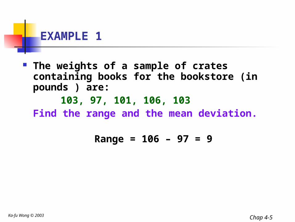
EXAMPLE 1

The weights of a sample of crates containing books for the bookstore (in pounds ) are:

103, 97, 101, 106, 103Find the range and the mean deviation.

Range = 106 – 97 = 9

Ka-fu Wong © 2003 Chap 4-6

Example 1

The first step is to find the mean weight.

The mean deviation is:

102=5

510=

nΣX

=X

2.4=5

5+4+1+5+1=

5102-103+...+102-103

=n

X-X Σ=MD

Ka-fu Wong © 2003 Chap 4-7

Population Variance

The population variance is the arithmetic mean of the squared deviations from the population mean.

All values are used in the calculation. More likely to be influenced by extreme

values than mean deviation. The units are awkward, the square of the

original units.

Ka-fu Wong © 2003 Chap 4-8

Variance

The formula for the population variance is:

The formula for the sample variance is:

Nμ)-Σ(X

=σ2

2

1-n)X-Σ(X

=s2

2

Note in the sample variance formula the sum of deviation is divided by (n-1) instead of n. Although it is logical to use n instead of (n-1), the division by (n-1) yields an unbiased estimator of the population variance but the division by n yields a biased estimator.

Ka-fu Wong © 2003 Chap 4-9

EXAMPLE 2

The ages of the Dunn family are: 2, 18, 34, 42

What is the population variance?

24=496

=nΣX

=μ

( ) ( )

236=4

944=

424-42+...+24-2

=N

μ)-Σ(X=σ

2222

Ka-fu Wong © 2003 Chap 4-10

The Population Standard Deviation

The population standard deviation (σ) is the square root of the population variance.

For EXAMPLE 2, the population standard deviation is 15.36, found by

15.36=236=σ=σ 2

Ka-fu Wong © 2003 Chap 4-11

EXAMPLE 3

The hourly wages earned by a sample of five students are:

$7, $5, $11, $8, $6. Find the variance.

7.40=537

=nΣX

=X

( ) ( ) ( )

5.30=1-5

21.2=

1-57.4-6+...+7.4-7

=1-nX-XΣ

=s222

2

Ka-fu Wong © 2003 Chap 4-12

Sample Standard Deviation

The sample standard deviation is the square root of the sample variance.

In EXAMPLE 3, the sample standard deviation is 2.30

2.30=5.29=s=s 2

Ka-fu Wong © 2003 Chap 4-13

Sample Variance For Grouped Data

The formula for the sample variance for grouped data is:

1-n

xn-Σfx

1-n

xnx2n-Σfx

1-n

xΣfΣfxx2-Σfx

1-n

)xxx2-Σf(x

1-Σf

)x-Σf(x=s

22

222

22

2222

Ka-fu Wong © 2003 Chap 4-14

Interpretation and Uses of the Standard Deviation

Chebyshev’s theorem: For any set of observations, the minimum proportion of the values that lie within k standard deviations of the mean is at least:

where k2 is any constant greater than 1.

2k1

-1

Ka-fu Wong © 2003 Chap 4-15

Chebyshev’s theorem

K Coverage

1 0%

2 75.00%

3 88.89%

4 93.75%

5 96.00%

6 97.22%

Chebyshev’s theorem: For any set of observations, the minimum proportion of the values that lie within k standard deviations of the mean is at least 1- 1/k2

Ka-fu Wong © 2003 Chap 4-16

Interpretation and Uses of the Standard Deviation

Empirical Rule: For any symmetrical, bell-shaped distribution: About 68% of the observations will lie within

1s the mean, About 95% of the observations will lie within

2s of the mean Virtually all the observations will be within

3s of the mean

Empirical rule is also known as normal rule.

Ka-fu Wong © 2003 Chap 4-17

Bell-shaped Curve showing the relationship between σ and μ

Ka-fu Wong © 2003 Chap 4-18

Why are we concern about dispersion?

Dispersion is used as a measure of risk. Consider two assets of the same expected

(mean) returns. -2%, 0%,+2% -4%, 0%,+4%

The dispersion of returns of the second asset is larger then the first. Thus, the second asset is more risky.

Thus, the knowledge of dispersion is essential for investment decision. And so is the knowledge of expected (mean) returns.

Ka-fu Wong © 2003 Chap 4-19

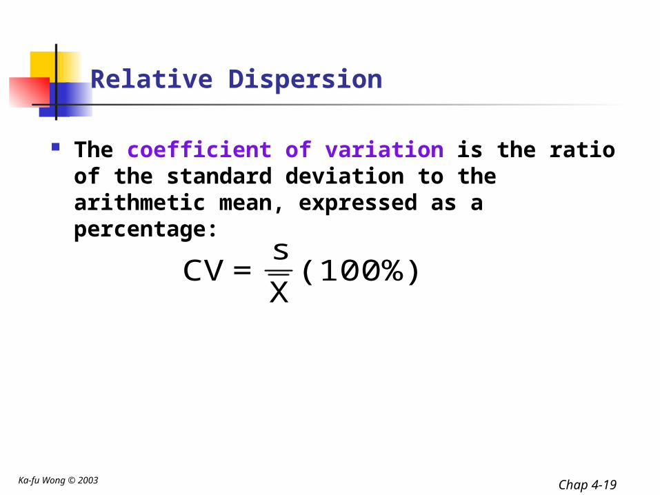
Relative Dispersion

The coefficient of variation is the ratio of the standard deviation to the arithmetic mean, expressed as a percentage:

(100%)X

s=CV

Ka-fu Wong © 2003 Chap 4-20

Sharpe Ratio and Relative Dispersion

Sharpe Ratio is often used to measure the performance of investment strategies, with an adjustment for risk.

If X is the return of an investment strategy in excess of the market portfolio, the inverse of the CV is the Sharpe Ratio.

An investment strategy of a higher Sharpe Ratio is preferred.

http://www.stanford.edu/~wfsharpe/art/sr/sr.htm

Ka-fu Wong © 2003 Chap 4-21

Skewness

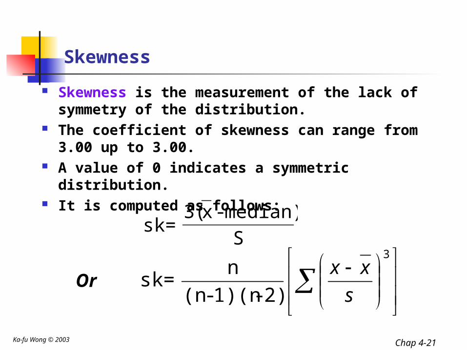
Skewness is the measurement of the lack of symmetry of the distribution.

The coefficient of skewness can range from 3.00 up to 3.00.

A value of 0 indicates a symmetric distribution.

It is computed as follows:

Smedian)-x3(

=sk

3

s

xx

2)-1)(n-(nn

=skOr

Ka-fu Wong © 2003 Chap 4-22

Why are we concerned about skewness?

Skewness measures the degree of asymmetry in risk. Upside risk Downside risk

Consider the distribution of asset returns: Right skewed implies higher upside risk

than downside risk. Left skewed implies higher downside risk

than upside risk.

Ka-fu Wong © 2003 Chap 4-23

Interquartile Range

The Interquartile range is the distance between the third quartile Q3 and the first quartile Q1.

This distance will include the middle 50 percent of the observations.

Interquartile range = Q3 - Q1

Ka-fu Wong © 2003 Chap 4-24

EXAMPLE 5

For a set of observations the third quartile is 24 and the first quartile is 10. What is the quartile deviation?

The interquartile range is 24 - 10 = 14. Fifty percent of the observations will occur between 10 and 24.

Ka-fu Wong © 2003 Chap 4-25

Box Plots

A box plot is a graphical display, based on quartiles, that helps to picture a set of data.

Five pieces of data are needed to construct a box plot: the Minimum Value, the First Quartile, the Median, the Third Quartile, and the Maximum Value.

Ka-fu Wong © 2003 Chap 4-26

EXAMPLE 6

Based on a sample of 20 deliveries, Buddy’s Pizza determined the following information. The minimum delivery time was 13 minutes and the maximum 30 minutes. The first quartile was 15 minutes, the median 18 minutes, and the third quartile 22 minutes. Develop a box plot for the delivery times.

Ka-fu Wong © 2003 Chap 4-27

EXAMPLE 6 continued

12 14 16 18 20 22 24 26 28 30 32

min max

median

Q1 Q3

Ka-fu Wong © 2003 Chap 4-28

Working with mean and Standard Deviation

Set DataMea

nSt Dev

(1) 19 20 2120.0

0 0.82

(2) -1 0 1 0.00 0.82

(3) 19 20 20 2120.0

0 0.71

(4) 38 40 4240.0

0 1.63

(5) 57 60 6360.0

0 2.45

(6) 19 19 20 20 21 2120.0

0 0.82

(7) 3 5 8 5.33 2.05

(8) 4 7 9 6.67 2.05

(9) 7 12 1712.0

0 4.08

(10)

12 20 21 27 32 35 45 56 7235.5

6 18.04

Ka-fu Wong © 2003 Chap 4-29

(2) = (1) – mean(1): Mean(2)=0; Stdev(2)=Stdev(1)

(3) = (1) + mean(1) Mean(3)=Mean(1); Stdev(3)<Stdev(1).

(4) = (1)*2; (5) = (1)*3 Mean(4)=mean(1)*2; mean(5)=mean(1)*3 Stdev(4)=stdev(1)*2; stdev(5)=stdev(1)*3

Working with mean and Standard Deviation

Set DataMea

nSt Dev

(1) 19 20 2120.0

0 0.82

(2) -1 0 1 0.00 0.82

(3) 19 20 20 2120.0

0 0.71

(4) 38 40 4240.0

0 1.63

(5) 57 60 6360.0

0 2.45

Ka-fu Wong © 2003 Chap 4-30

Working with mean and Standard Deviation

Set DataMea

nSt Dev

(1) 19 20 2120.0

0 0.82

(6) 19 19 20 20 21 2120.0

0 0.82

(7) 3 5 8 5.33 2.05

(8) 4 7 9 6.67 2.05

(9) 7 12 1712.0

0 4.08

(10)

12 20 21 27 32 35 45 56 7235.5

6 18.04

(6)=(1) multiplied by some frequency Mean(6)=Mean(1); Stdev(6)=Stdev(1).

(9) = (7)+(8) Mean(9)=mean(7)+mean(8)

(10) = (7) *(8) Mean(10)=mean(7)*mean(8)

Ka-fu Wong © 2003 Chap 4-31

Further results about mean and variance of transformed

variables

E(X) = mean or expected values V(X) = E[(X-E(X))2]=E(X2) – E(X)2 E(a+bX) = a+bE(X) E(X+Y) = E(X) + E(Y) V(X+Y) = V(X) + V(Y) if X and Y are

independent.

Ka-fu Wong © 2003 Chap 4-32

Further results about mean and variance of transformed

variables

E(a+bX) = a+bE(X) E(X+Y) = E(X) + E(Y) Suppose we invest $1 in two assets. $a in

asset X and $(1-a) in asset Y. Their expected returns are respectively E(X) and E(Y). We will expect a return of E(aX+(1-a)Y) = aE(X) + (1-a)E(Y) for this investment portfolio.

If these two assets are independent or uncorrelated so that C(X,Y) =0, then the variance is V(aX+(1-a)Y) = a2V(X) + (1-a)2V(Y)

Ka-fu Wong © 2003 Chap 4-33

- END -

Chapter FourOther Descriptive Measures Other Descriptive Measures (dispersion)(dispersion)