JMLR Workshop and Conference Proceedings Volume 10: Feature Selection in Data Mining Proceedings of the Fourth International Workshop on Feature Selection in Data Mining, June 21st, 2010, Hyderabad, India Editors: Huan Liu, Hiroshi Motoda, Rudy Setiono, Zheng Zhao Preface Huan Liu, Hiroshi Motoda, Rudy Setiono, Zheng Zhao; 10: 1-3, 2010. Feature Selection: An Ever Evolving Frontier in Data Mining Huan Liu, Hiroshi Motoda, Rudy Setiono, Zheng Zhao; 10:4-13, 2010. Feature Selection, Association Rules Network and Theory Building Sanjay Chawla; 10:14-21, 2010. A Statistical Implicative Analysis Based Algorithm and MMPC Algorithm for Detecting Multiple Dependencies Elham Salehi, Jayashree Nyayachavadi and Robin Gras; 10:22-34, 2010. Attribute Selection Based on FRiS-Compactness Nikolay Zagoruiko, Irina Borisova, Vladimir Dyubanov and Olga Kutnenko; 10:35-44, 2010. Effective Wrapper-Filter hybridization through GRASP Schemata Mohamed Amir Esseghir; 10:45-54, 2010. Feature Extraction for Machine Learning: Logic-Probabilistic Approach Vladimir Gorodetsky and Vladimir Samoylov; 10:55-65, 2010. Feature Extraction for Outlier Detection in High-Dimensional Spaces Hoang Vu Nguyen and Vivekanand Gopalkrishnan; 10:66-75, 2010. Feature Selection for Text Classification Based on Gini Coefficient of Inequality Ranbir Sanasam, Hema Murthy and Timothy Gonsalves; 10:76-85, 2010. Increasing Feature Selection Accuracy for L1 Regularized Linear Models Abhishek Jaiantilal and Gregory Grudic; 10:86-96, 2010. Learning Dissimilarities for Categorical Symbols Jierui Xie, Boleslaw Szymanski and Mohammed Zaki; 10:97-106, 2010.

Welcome message from author
This document is posted to help you gain knowledge. Please leave a comment to let me know what you think about it! Share it to your friends and learn new things together.
Transcript

JMLR Workshop and Conference Proceedings Volume 10: Feature Selection in Data Mining
Proceedings of the Fourth International Workshop on Feature Selection in Data Mining, June 21st, 2010, Hyderabad, India
Editors: Huan Liu, Hiroshi Motoda, Rudy Setiono, Zheng Zhao
Preface
Huan Liu, Hiroshi Motoda, Rudy Setiono, Zheng Zhao; 10: 1-3, 2010.
Feature Selection: An Ever Evolving Frontier in Data Mining
Huan Liu, Hiroshi Motoda, Rudy Setiono, Zheng Zhao; 10:4-13, 2010.
Feature Selection, Association Rules Network and Theory Building
Sanjay Chawla; 10:14-21, 2010.
A Statistical Implicative Analysis Based Algorithm and MMPC Algorithm for Detecting Multiple Dependencies
Elham Salehi, Jayashree Nyayachavadi and Robin Gras; 10:22-34, 2010.
Attribute Selection Based on FRiS-Compactness
Nikolay Zagoruiko, Irina Borisova, Vladimir Dyubanov and Olga Kutnenko; 10:35-44, 2010.
Effective Wrapper-Filter hybridization through GRASP Schemata
Mohamed Amir Esseghir; 10:45-54, 2010.
Feature Extraction for Machine Learning: Logic-Probabilistic Approach
Vladimir Gorodetsky and Vladimir Samoylov; 10:55-65, 2010.
Feature Extraction for Outlier Detection in High-Dimensional Spaces
Hoang Vu Nguyen and Vivekanand Gopalkrishnan; 10:66-75, 2010.
Feature Selection for Text Classification Based on Gini Coefficient of Inequality
Ranbir Sanasam, Hema Murthy and Timothy Gonsalves; 10:76-85, 2010.
Increasing Feature Selection Accuracy for L1 Regularized Linear Models
Abhishek Jaiantilal and Gregory Grudic; 10:86-96, 2010.
Learning Dissimilarities for Categorical Symbols
Jierui Xie, Boleslaw Szymanski and Mohammed Zaki; 10:97-106, 2010.

JMLR: Workshop and Conference Proceedings 10: 1-3 The Fourth Workshop on Feature Selection in Data Mining
Preface
Welcome to FSDM’10
Knowledge discovery and data mining (KDD) is a multidisciplinary field that researches anddevelops theories, algorithms and software systems to mine gold nuggets of knowledge fromdata. The increasingly large data sets from many application domains have posed renewedchallenges to KDD; in the meantime, new types of data are evolving such as social media,text, and microarray data. Researchers and practitioners in multiple disciplines and variousIT sectors confront similar issues in feature selection, and there is still a pressing need forcontinued exchange and discussion of challenges and ideas, exploring new methodologiesand innovative approaches in search of breakthroughs.
Feature selection is effective in data preprocessing and reduction, thus is an essential step insuccessful data mining applications. Feature selection has been a research topic with practi-cal significance in many areas such as statistics, pattern recognition, machine learning, anddata mining (including Web, text, image, and microarrays). The objectives of feature se-lection include: building simpler and more comprehensible models, improving data miningperformance, and helping prepare, clean, and understand data. The Workshop on FeatureSelection in Data Mining (FSDM) aims to further the cross-discipline, collaborative effortin feature (a.k.a. variable) selection research and application. This year, FSDM is heldwith the 14th Pacific-Asia Conference on Knowledge Discovery and Data Mining (PAKDD2010) in Hyderabad, India.
FSDM’10 consists of one keynote speech and 8 peer-reviewed papers. in which four papersare on developing new algorithms or improving existing algorithms of feature selection; twopapers on designing effective feature selection algorithms for real-world problems; and threepapers on exploring novel problems in feature selection research.
It has been an enjoyable journey for us to work together with program committee mem-bers and authors to make this workshop a reality. We would like to convey our immensegratitude to the PC members for spending their precious time helping review and selectpapers, and to all the authors for their contributions and efforts in generating the FSDM’10proceedings. Last but not least, we would like to thank Neil Lawrence from JMLR, andthe organizers of PAKDD for their guidance and help in producing the proceedings and inorganizing this workshop.
Huan Liu, Hiroshi Motoda, Rudy Setiono, Zheng Zhao
June 21, Hyderabad, India
c©2010 Liu, Motoda, Setiono and Zhao.

Liu, Motoda, Setiono and Zhao
FSDM’10 Workshop Chairs
• Huan Liu (Arizona State University)
• Hiroshi Motoda (Osaka University)
• Rudy Setiono (National University of Singapore)
• Zheng Zhao (Arizona State University)
Workshop Program Committee
• Constantin Aliferis (Langone Medical Center, USA)
• leonardo auslender (SAS Institute, USA)
• Selin Aviyente (Michigan State University, USA)
• Gianluca Bontempi (Universite Libre de Bruxelles, Belgium)
• Zheng Chen (Microsoft Research Asia, China)
• Soon Chung (Wright State University, USA)
• Anirban Dasgupta (Yahoo! Research, USA)
• Manoranjan Dash (Nanyang Technological University, Singapore)
• Petros Drineas (Rensselaer Polytechnic Institute, USA)
• Pierre Dupont (University catholique de Louvain, Belgium)
• Wei Fan (IBM Watson, USA)
• Assaf Gottlieb (Tel Aviv University, Israel)
• Mark Hall (University of Waikato, New Zealand)
• Michael E. Houle (National Institute of Informatics, Japan)
• D. Frank Hsu (Fordham University, USA)
• Inaki Inza (University of the Basque Country, Spain)
• Rong Jin (Michigan State University, USA)
• Irwin King (The Chinese University of Hong Kong)
• Jacek Koronacki (Institute of Computer Science, Polish Acad. Sci., Porland)
• Igor Kononenko (University of Ljubljana, Slovenia)
• Mineichi Kudo (Hokkaido University, Japan)
2

Preface
• James Kwok (Hong Kong University of Science and Technology, China)
• Yanjun Li (Fordham University, USA)
• Huan Liu (Arizona State University, USA)
• xiaohui liu (Brunel University, UK)
• Fabricio M. Lopes (Federal University of Technology - Parana, Brazil)
• Kezhi Mao (Nanyang Technological University, Singapore)
• Elena Marchiori (Radboud University, Netherlands)
• Hiroshi Motota (Osaka University and AFOSR/AOARD, Japan)
• Satoshi Niijima (Kyoto University, Japan)
• Tao Qin (Tsinghua University, China)
• Chai quek (Nanyang Technological University, Singapore)
• Marko Robnik-Sikonja (University of Ljubljana, FRI, Slovenia)
• Yvan Saeys (Ghent University, Belgium)
• Rudy Setiono (National University of Singapore)
• Jian-Tao Sun (Microsoft Research Asia, China)
• Ioannis Tsamardinos (University of Crete, Greece)
• Fei Wang (IBM Almaden Research Center, USA)
• Lei Wang (The Australian National University, Australia)
• Louis Wehenkel (University of Liege, Belgium)
• Zenglin Xu (Chinese University of Hong Kong, China)
• Jieping Ye (Arizona State University, USA)
• Lei Yu (Binghamton University, USA)
• Kun Zhang (Xavier University of Louisiana, USA)
Workshop web site
http://featureselection.asu.edu/fsdm10/index.html
3
JMLR: Workshop and Conference Proceedings 10: 4-13 The Fourth Workshop on Feature Selection in Data Mining
Feature Selection: An Ever Evolving Frontier in Data Mining
Huan Liu [email protected] Science and Engineering,Arizona State University, USA
Hiroshi Motoda [email protected] Office of Aerospace Research and Development,Air Force Office of Scientific Research,US Air Force Research Laboratory, JAPANand Institute of Scientific Research,Osaka University , JAPAN
Rudy Setiono [email protected] of Computing,National University of Singapore, SINGAPORE
Zheng Zhao [email protected]
Computer Science and Engineering,
Arizona State University, USA
Editor: Neil Lawrence
Abstract
The rapid advance of computer technologies in data processing, collection, and storage hasprovided unparalleled opportunities to expand capabilities in production, services, commu-nications, and research. However, immense quantities of high-dimensional data renew thechallenges to the state-of-the-art data mining techniques. Feature selection is an effectivetechnique for dimension reduction and an essential step in successful data mining appli-cations. It is a research area of great practical significance and has been developed andevolved to answer the challenges due to data of increasingly high dimensionality. Its directbenefits include: building simpler and more comprehensible models, improving data miningperformance, and helping prepare, clean, and understand data. We first briefly introducethe key components of feature selection, and review its developments with the growth ofdata mining. We then overview FSDM and the papers of FSDM10, which showcases of a vi-brant research field of some contemporary interests, new applications, and ongoing researchefforts. We then examine nascent demands in data-intensive applications and identify somepotential lines of research that require multidisciplinary efforts.
Keywords: Feature Selection, Feature Extraction, Dimension Reduction, Data Mining
1. An Introduction to Feature Selection
Data mining is a multidisciplinary effort to extract nuggets of knowledge from data. Theproliferation of large data sets within many domains poses unprecedented challenges todata mining (Han and Kamber, 2001). Not only are data sets getting larger, but newtypes of data become prevalent, such as data streams on the Web, microarrays in genomics
c©2010 Liu, Motoda, Setiono, and Zhao.

Feature Selection: An Ever Evolving Frontier in Data Mining
and proteomics, and networks in social computing and system biology. Researchers arerealizing that in order to achieve successful data mining, feature selection is an indispensablecomponent (Liu and Motoda, 1998; Guyon and Elisseeff, 2003; Liu and Motoda, 2007). Itis a process of selecting a subset of original features according to certain criteria, andan important and frequently used technique in data mining for dimension reduction. Itreduces the number of features, removes irrelevant, redundant, or noisy features, and bringsabout palpable effects for applications: speeding up a data mining algorithm, improvinglearning accuracy, and leading to better model comprehensibility. Various studies showthat some features can be removed without performance deterioration (Ng, 2004; Donoho,2006). Feature selection has been an active field of research for decades in data mining,and has been widely applied to many fields such as genomic analysis (Inza et al., 2004),text mining (Forman, 2003), image retrieval (Gonzalez and Woods, 1993; Swets and Weng,1995), intrusion detection (Lee et al., 2000), to name a few. As new applications emerge inrecent years, many challenges arise requiring novel theories and methods addressing high-dimensional and complex data. Feature selection for data of ultrahigh dimensionality (Fanet al., 2009), steam data (Glocer et al., 2005), multi-task data (Liu et al., 2009; G. Obozinskiand Jordan, 2006), and multi-source data (Zhao et al., 2008, 2010a) are among emergingresearch topics of pressing needs.
EvaluationFeature Subset
Generation
Training
Data
Stop
Criterion
NO
Feature Selection
Training
Learning Model
Yes
Best SubsetTest Learning
ModelTest Data
ACC Model Fitting/Performance Evaluation
phase I
phase II
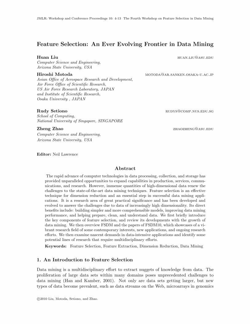
Figure 1: A unified view of a feature selection process
Figure 1 presents a unified view for a feature selection process. A typical feature se-lection process contains two phases: feature selection, and model fitting and performanceevaluation. The feature selection phase contains three steps: (1) generating a candidate setcontaining a subset of the original features via certain research strategies; (2) evaluatingthe candidate set and estimating the utility of the features in the candidate set. Basedon the evaluation, some features in the candidate set may be discarded or added to theselected feature set according to their relevance; and (3) determining whether the current
5
Liu, Motoda, Setiono, and Zhao
set of selected features are good enough using certain stopping criterion. If it is, a featureselection algorithm will return the set of selected features, otherwise, it iterates until thestopping criterion is met. In the process of generating the candidate set and evaluating it, afeature selection algorithm may use the information from the training data, current selectedfeatures, target learning model, and given prior knowledge (Helleputte and Dupont, 2009)to guide their search and evaluation. Once a set of features is selected, it can be used tofilter the training and test data for model fitting and prediction. The performance achievedby a particular learning model on the test data can also be used to as an indicator forevaluating the effectiveness of the feature selection algorithm for that learning model.
In the process of feature selection, the training data can be either labeled, unlabeledor partially labeled, leading to the development of supervised, unsupervised and semi-supervised feature selection algorithms. In the evaluation process, a supervised featureselection algorithm (Sikonja and Kononenko, 2003; Weston et al., 2003; Song et al., 2007;Zhang et al., 2008) determines features’ relevance by evaluating their correlation with theclass or their utility for achieving accurate predication, and without labels, an unsupervisedfeature selection algorithm may exploit data variance or data distribution in its evaluationof features’ relevance (Dash and Liu, 2000; Dy and Brodley, 2004; He et al., 2005). A semi-supervised feature selection algorithm (Zhao and Liu, 2007c; Xu et al., 2009) uses a smallamount of labeled data as additional information to improve unsupervised feature selection.
Depending on how and when the utility of selected features is evaluated, different strate-gies can be adopted, which broadly fall into three categories: filter, wrapper and embed-ded models. To evaluate the utility of features, in the evaluation step, feature selectionalgorithms of filter model rely on analyzing the general characteristics of data and evaluatingfeatures without involving any learning algorithm. On the other hand, feature selection algo-rithms of wapper model require a predetermined learning algorithm and use its performanceon the provided features in the evaluation step to identify relevant feature. Algorithms ofthe embedded model, e.g., C4.5 (Quinlan, 1993), LARS (Efron et al., 2004), 1-norm sup-port vector machine (Zhu et al., 2003), and sparse logistic regression (Cawley et al., 2007),incorporate feature selection as a part of the model fitting/training process, and features’utility is obtained based on analyzing their utility for optimizing the objective function ofthe learning model. Compared to the wrapper and embedded models, algorithms of thefilter model are independent of any learning model, therefore do not have bias associatedwith any learning models, one advantage of the filter model. Another advantage of the filtermodel is that it allows the algorithms to have very simple structure, which usually employsa straightforward search strategy, such as backward elimination or forward selection, anda feature evaluation criterion designed according to certain criterion. The benefit of thesimple structure is two-folds. First, it is easy to design, and after it is implemented, itis also easy to understand for other researchers. This actually explains why most featureselection algorithms are of the filter model. And in real world applications, many mostfrequently used feature selection algorithms are also filters. Second, since the structure ofthe algorithms is simple, they are usually very fast. On the other hand, researcher alsorecognized that compared to the filter model, feature selection algorithms of the wrapperand embedded models can usually select features that result in higher learning performancefor a particular learning model, which is used in the feature selection process. Comparingwith the wrapper model, feature selection algorithms of embedded model are usually more
6

Feature Selection: An Ever Evolving Frontier in Data Mining
efficient, since they look into the structure of the involved learning model and use its proper-ties to guide feature evaluation and search. In recent years, the embedded model is gainingincreasing interests in feature selection research due to its superior performance. Currently,most embedded feature selection algorithms are designed by applying L0 norm (Westonet al., 2003; Huang et al., 2008) or L1 norm (Liu et al., 2009; Zhu et al., 2003; Zhao et al.,2010b) as a constraint to existing learning models to achieve a sparse solution. When theconstraint is of L1 norm form, and the original problem is convex, existing optimizationtechniques can be applied to obtain the unique global optimal solution for the regularizedproblem in a very efficient way (Liu et al., 2009).
Feature selection algorithms with the filter and embedded models may return either asubset of selected features or the weights (measuring features’ relevance) of all features.According to the type of the output, feature selection algorithms can be divided into ei-ther feature weighting algorithms or subset selection algorithms. Feature selectionalgorithms of the wrapper model usually return feature subsets, therefore are subset selec-tion algorithms. To the best of our knowledge, currently, most feature selection algorithmsare designed to handle learning tasks with single data source. Researchers have startedexploring the capability of using multiple auxiliary data and prior knowledge sources formulti-source feature selection (Zhao and Liu, 2008) to effectively enhance the reliabilityof relevance estimation (Lu et al., 2005; Zhao et al., 2008, 2010a).
Given a rich literature exists for feature selection research, a systematical summariza-tion and comparison studies are of necessity to facilitate the research and application offeature selection techniques. Recently, there have been many surveys published to servethis purpose. A comprehensive surveys of existing feature selection techniques and a gen-eral framework for their unification can be found in (Liu and Yu, 2005). Guyon and Elis-seeff (2003) reviewed feature selection algorithms from statistical learning point of view.In (Saeys et al., 2007), the authors provided a good survey for applying feature selectiontechniques in bioinformatics. In (Inza et al., 2004), the authors reviewed and comparedthe filter with the wrapper model for feature selection. In (Ma and Huang, 2008), theauthors explored the representative feature selection approaches based on sparse regular-ization, which is a branch of embedded feature selection techniques. Representative featureselection algorithms are also empirically evaluated in (Liu et al., 2002; Li et al., 2004; Sunet al., 2005; Lai et al., 2006; Ma, 2006; Swartz et al., 2008; Murie et al., 2009) under differentproblem settings and from different perspectives. We refer readers to these survey works toobtain comprehensive understanding on feature selection research.
2. Toward Cross-Discipline Collaboration in Feature Selection Research
Knowledge discovery and data mining (KDD) is a multidisciplinary effort. Researchersand practitioners in multiple disciplines and various IT sectors confront similar issues infeature selection, and there is a pressing need for continuous exchange and discussion ofchallenges and ideas, exploring new methodologies and innovative approaches. The inter-national workshop on Feature Selection in Data Mining (FSDM) serves as a platform tofurther the cross-discipline, collaborative effort in feature selection research. FSDM 20051
1. http://enpub.fulton.asu.edu/workshop/
7

Liu, Motoda, Setiono, and Zhao
and 20062 were held with the SIAM Conference on Data Mining (SDM) 2005 and 2006,respectively. FSDM 20083 was held with the European Conference on Machine Learningand Principles and Practice of Knowledge Discovery in Databases (ECML/PKDD) 2008.And FSDM 20104 is the fourth workshop of this series, and is held at the 14th Pacific-AsiaConference on Knowledge Discovery and Data Mining (PAKDD) 2010. This collection con-sists of one keynote and 8 peer-reviewed papers, among which, there are three on exploringnovel problems in feature selection research; four on developing new feature selection algo-rithms or improving existing ones; two on designing effective algorithms to solve real-worldproblems. Below we give an overview on the papers of FSDM 2010.
Two novel feature selection research problems are investigated. In the keynote pa-per (Chawla, 2010), the author studies the interesting research problem of detecting featuredependence, which is also the topic of (Salehi et al., 2010). Both works are based on thetechniques related to association rule mining. A concept that is closely related to feature de-pendence is feature interaction, in which a set of features cooperate with each other to definethe target concept. The problem of feature interaction is studied in (Jakulin and Bratko,2004; Zhao and Liu, 2007b). Besides detecting feature dependence, the problem of featureextraction for heterogeneous data with ontology information is also studied in (Gorodetskyand Samoylov, 2010). It is an interesting feature extraction problem related to informationfusion and multi-source feature selection (Zhao and Liu, 2008).
The filter, wrapper, and embedded models are the major models used in feature selec-tion for algorithm design. In (Esseghir, 2010), an interesting hybrid approach is proposed tocombine the wrapper with the filter model through a so-called greedy randomized adaptivesearch procedure (GRASP). The advantage of the method is that it can inherit the strengthof both models to improve the performance of feature selection. In (Jaiantilal and Grudic,2010), a new feature selection algorithm based on the embedded model is proposed. Theintrinsic point of the paper is to develop a random sampling framework, which can effec-tively estimate feature weights for weighted L1 penalty based sparse learning models (Zou,2006). The pairwise sample similarity is an important way to depict the relationships amongsamples, and has been widely used in designing feature selection algorithms (Zhao and Liu,2007a). Improving the quality of similarity measurements is beneficial to the feature selec-tion algorithms by taking sample similarity as their input. In (Zagoruiko et al., 2010), theauthors propose to apply FRiS-function to improve similarity estimation. And in (Xie et al.,2010), the authors proposed to construct continuous variables from categorical features toachieve better similarity estimation.
Text mining is an important research area, where feature selection is widely applied fordimension reduction. In (Singh et al., 2010), the authors develop a new feature evaluationcriterion for text mining based on Gini coefficient of inequality. Their empirical studyshows that the proposed criterion significantly improve the learning performance comparedto several existing criteria in feature selection, including mutual information, informationgain and chi-square statistic. Besides text mining, feature extraction for outlier detectionis also studied. In (Nguyen and Gopalkrishnan, 2010), the authors propose to use weightadjusted scatter matrices in feature extraction to address the class unbalance issue in outlier
2. http://enpub.fulton.asu.edu/workshop/2006/3. http://www.psb.ugent.be/ yvsae/fsdm08/index.html4. http://featureselection.asu.edu/fsdm10/index.html
8

Feature Selection: An Ever Evolving Frontier in Data Mining
detection, and empirical results show that the proposed method can bring about nontrivialimprovement over the existing algorithms.
3. Advancing Feature Selection Research
The current development in scientific research will lead to the prevalence of ultrahigh di-mensional data generated from the high-throughput techniques (Fan et al., 2009) and theavailability of many useful knowledge sources resulting from collective work of cutting-edgeresearch. Hence one important research topic in feature selection is to develop computa-tional theories that help scientists to keep up with the rapid advance of new technologieson data collection and processing. We also notice that there is a chasm between symboliclearning and statistical learning that prevents scientists from taking advantage of data andknowledge in a seamless way. Symbolic learning works well with knowledge and statisti-cal learning works with data. Explanation-based learning is one such example that wouldprovide an efficient way to bridge this gap. The technique of explanation-based featureselection will enable us to use the accumulated domain knowledge to help narrow downthe search space and explain the learning results by providing reasons why certain featuresare relevant. Below are our conjectures about some interesting research topics in featureselection of potential impact in the near future.
Feature selection for ultrahigh dimensional data: selecting features on data sets withmillions of features (Fan et al., 2009). As high-throughput techniques keep evolving, manycontemporary research projects in scientific discovery generate data with ultrahigh dimen-sionality. For instance, the next-generation sequencing techniques in genetics analysis cangenerate data with several giga features on one run. Computation inherent in existingmethods makes them hard to directly handle data of such high dimensionality, which raisesthe simultaneous challenges of computational power, statistical accuracy, and algorithmicstability. To address these challenges, researchers need to develop efficient approaches forfast relevance estimation and dimension reduction. Prior knowledge can play an importantrole in this study, for example, by providing effective ways to partition original feature spaceto subspaces, which leads to significant reduction on search space and allows the applicationof highly efficient parallel techniques.
Knowledge oriented sparse learning: fitting sparse learning models via utilizing multipletypes of knowledge. This direction extends multi-source feature selection (Zhao and Liu,2008). Sparse learning allows joint model fitting and features selection. Given multipletypes of knowledge, researchers need to study how to use knowledge to guide inference forimproving learning performance, such as the prediction accuracy, and model interpretabil-ity. For instance, in microarray analysis, given gene regulatory network and gene ontologyannotation, it is interesting to study how to simultaneously infer with both types of knowl-edge, for example, via network dynamic analysis or function concordance analysis, to buildaccurate prediction models based on a compact set of genes. One direct benefit of utilizingexisting knowledge in inference is that it can significantly increase the reliability of the rel-evance estimation (Zhao et al., 2010a). Another benefit of using knowledge is that it mayreduce cost by requiring fewer samples for model fitting.
Explanation-based feature selection (EBFS): feature selection via explaining trainingsamples using concepts generalized from existing features and knowledge. In many real-
9
Liu, Motoda, Setiono, and Zhao
world applications, the same phenomenon might be caused by disparate reasons. For ex-ample, in a cancer study, a certain phenotype may be related to mutations of either genesA or gene B in the same functional module M. And both gene A and gene B can cause thedefect of M. Existing feature selection algorithm based on checking feature/class correla-tion may not work in this situation, due to the inconsistent (variable) expression patternof gene A and gene B across the cancerous samples5. The generalization step in EBFScan effectively screen this variation by forming high-level concepts via using the ontologyinformation obtained from annotation databases, such as GO. Another advantage of EBFSis that it can generate sensible explanations to show why the selected features are related.EBFS is related to the research of explanation-based learning (EBL) and relational learning.
Feature selection remains and will continue to be an active field that is incessantlyrejuvenating itself to answer new challenges.
Acknowledgments
This work is, in part, supported by NSF Grant (0812551).
References
G. C. Cawley, N. L. C. Talbot, and M. Girolami. Sparse multinomial logistic regression viabayesian l1 regularisation. In NIPS, 2007.
Sanjay Chawla. Feature selection, association rules network and theory building. In The4th Workshop on Feature Selection in Data Mining, 2010.
M. Dash and H. Liu. Feature selection for clustering. In Proceedings of 4th Pacific AsiaConference on Knowledge Discovery and Data Mining, 2000. Springer-Verlag, 2000.
D. Donoho. Formost large underdetermined systems of linear equations, the minimal l1-norm solution is also the sparsest solution. Comm. Pure Appl. Math., 59:907–934, 2006.
Jennifer G. Dy and Carla E. Brodley. Feature selection for unsupervised learning. J. Mach.Learn. Res., 5:845–889, 2004. ISSN 1533-7928.
B. Efron, T. Hastie, I. Johnstone, and R. Tibshirani. Least angle regression. Annals ofStatistics, 32:407–49, 2004.
M. A. Esseghir. Effective wrapper-filter hybridization through grasp schemata. In The 4thWorkshop on Feature Selection in Data Mining, 2010.
Jianqing Fan, Richard Samworth, and Yichao Wu. Ultrahigh dimensional feature selection:Beyond the linear model. Journal of Machine Learning Research, 10:2013–2038, 2009.
George Forman. An extensive empirical study of feature selection metrics for text classifi-cation. Journal of Machine Learning Research, 3:1289–1305, 2003.
B. Taskar G. Obozinski and M. I. Jordan. Multi-task feature selection. Technical report,Statistics Department, UC Berkeley, 2006.
5. For a cancerous sample, either gene A or gene B has abnormal expression, but not both.
10

Feature Selection: An Ever Evolving Frontier in Data Mining
K. Glocer, D. Eads, and J. Theiler. Online feature selection for pixel classification. InProceedings of the 22nd international conference on Machine learning (ICML), 2005.
R. Gonzalez and R. Woods. Digital Image Processing. Addison-Wesley, 2nd edition, 1993.
V. Gorodetsky and V. Samoylov. Feature extraction for machine learning: Logic-probabilistic approach. In The 4th Workshop on Feature Selection in Data Mining, 2010.
I. Guyon and A. Elisseeff. An introduction to variable and feature selection. Journal ofMachine Learning Research, 3:1157–1182, 2003.
J. Han and M. Kamber. Data Mining: Concepts and Techniques. Morgan Kaufman, 2001.
X. He, D. Cai, and P. Niyogi. Laplacian score for feature selection. Advances in NeuralInformation Processing Systems 18, Cambridge, MA, 2005. MIT Press.
Thibault Helleputte and Pierre Dupont. Partially supervised feature selection with regu-larized linear models. In ICML, 2009.
Kaizhu Huang, Irwin King, and Michael R. Lyu. Direct zero-norm optimization for featureselection. In Proceeding of The 8th IEEE International Conference on Data Mining, 2008.
I. Inza, P. Larranaga, R. Blanco, and A. Cerrolaza. Filter versus wrapper gene selection ap-proaches in dna microarray domains. Artificial Intelligence in Medicine, 31:91–103,2004.
A. Jaiantilal and G. Grudic. Increasing feature selection accuracy for l1 regularized linearmodels in large datasets. In the 4th Workshop on Feature Selection in Data Mining, 2010.
A. Jakulin and I. Bratko. Testing the significance of attribute interactions. In ICML, 2004.
Carmen Lai, Marcel J T Reinders, Laura J van’t Veer, and Lodewyk F A Wessels. Acomparison of univariate and multivariate gene selection techniques for classification ofcancer datasets. BMC Bioinformatics, 7:235, 2006.
W. Lee, S. J. Stolfo, and K. W. Mok. Adaptive intrusion detection: A data mining approach.AI Review, 14(6):533 – 567, 2000.
Tao Li, Chengliang Zhang, and Mitsunori Ogihara. A comparative study of feature selectionand multiclass classification methods for tissue classification based on gene expression.Bioinformatics, 20(15):2429–2437, 2004.
H. Liu and H. Motoda. Feature Selection for Knowledge Discovery and Data Mining. Boston:Kluwer Academic Publishers, 1998. ISBN 0-7923-8198-X.
H. Liu and H. Motoda, editors. Computational Methods of Feature Selection. Chapmanand Hall/CRC Press, 2007.
H. Liu and L. Yu. Toward integrating feature selection algorithms for classification andclustering. IEEE Trans. on Knowledge and Data Engineering, 17(3):1–12, 2005.
11

Liu, Motoda, Setiono, and Zhao
Huiqing Liu, Jinyan Li, and Limsoon Wong. A comparative study on feature selection andclassification methods using gene expression profiles and proteomic patterns. GenomeInform, 13:51–60, 2002.
J. Liu, S. Ji, and J. Ye. Multi-task feature learning via efficient l2,1-norm minimization. Inthe Twenty-Fifth Conference on Uncertainty in Artificial Intelligence, 2009.
J. Lu, G. Getz, E. A. Miska, E. Alvarez-Saavedra, J. Lamb, D. Peck, A. Sweet-Cordero,B. L. Ebert, R. H. Mak, A. Ferrando, J. R. Downing, T. Jacks, H. R. Horvitz, and T. R.Golub. Microrna expression profiles classify human cancers. Nature, 435:834–838, 2005.
S. Ma. Empirical study of supervised gene screening. BMC Bioinformatics, 7:537, 2006.
Shuangge Ma and Jian Huang. Penalized feature selection and classification in bioinformat-ics. Brief Bioinform, 9(5):392–403, Sep 2008.
Carl Murie, Owen Woody, Anna Lee, and Robert Nadon. Comparison of small n statisticaltests of differential expression applied to microarrays. BMC Bioinformatics, 10:45, 2009.
A. Y. Ng. Feature selection, l1 vs. l2 regularization, and rotational invariance. In the 21stinternational conference on Machine learning. ACM Press, 2004.
H. V. Nguyen and V. Gopalkrishnan. Feature extraction for outlier detection in high-dimensional spaces. In The 4th Workshop on Feature Selection in Data Mining, 2010.
J. R. Quinlan. C4.5: Programs for Machine Learning. Morgan Kaufmann, 1993.
Yvan Saeys, Iaki Inza, and Pedro Larraaga. A review of feature selection techniques inbioinformatics. Bioinformatics, 23(19):2507–2517, 2007.
Elham Salehi, Jayashree Nyayachavadi, and Robin Gras. A statistical implicative analysisbased algorithm and mmpc algorithm for detecting multiple dependencies. In The 4thWorkshop on Feature Selection in Data Mining, 2010.
M. R. Sikonja and I. Kononenko. Theoretical and empirical analysis of Relief and ReliefF.Machine Learning, 53:23–69, 2003.
Sanasam Ranbir Singh, Hema A. Murthy, and Timothy A. Gonsalves. Feature selection fortext classification based on gini coecient of inequality. In The 4th Workshop on FeatureSelection in Data Mining, 2010.
L. Song, A. Smola, A. Gretton, K. Borgwardt, and J. Bedo. Supervised feature selectionvia dependence estimation. In International Conference on Machine Learning, 2007.
Y. Sun, C. F. Babbs, and E. J. Delp. A comparison of feature selection methods forthe detection of breast cancers in mammograms: adaptive sequential floating search vs.genetic algorithm. Conf Proc IEEE Eng Med Biol Soc, 6:6532–6535, 2005.
Michael D Swartz, Robert K Yu, and Sanjay Shete. Finding factors influencing risk: Com-paring bayesian stochastic search and standard variable selection methods applied tologistic regression models of cases and controls. Stat Med, 27(29):6158–6174, Dec 2008.
12

Feature Selection: An Ever Evolving Frontier in Data Mining
D. L. Swets and J. J. Weng. Efficient content-based image retrieval using automatic featureselection. In IEEE International Symposium On Computer Vision, pages 85–90, 1995.
J. Weston, A. Elisseff, B. Schoelkopf, and M. Tipping. Use of the zero norm with linearmodels and kernel methods. Journal of Machine Learning Research, 3:1439–1461, 2003.
Jierui Xie, Boleslaw Szymanski, and Mohammed J. Zaki. Learning dissimilarities for cate-gorical symbols. In The 4th Workshop on Feature Selection in Data Mining, 2010.
Zenglin Xu, Rong Jin, Jieping Ye, Michael R. Lyu, and Irwin King. Discriminative semi-supervised feature selection via manifold regularization. In IJCAI’ 09: Proceedings of the21th International Joint Conference on Artificial Intelligence, 2009.
Nikolai G. Zagoruiko, Irina A. Borisova, Vladimir V. Duybanov, and Olga A. Kutnenko.Attribute selection based on fris-compactness. In The 4th Workshop on Feature Selectionin Data Mining, 2010.
Yi Zhang, Chris Ding, and Tao Li. Gene selection algorithm by combining relieff and mrmr.BMC Genomics, 9:S27, 2008.
Z. Zhao and H. Liu. Spectral feature selection for supervised and unsupervised learning. InInternational Conference on Machine Learning (ICML), 2007
Z. Zhao, J. Wang, H. Liu, J. Ye, and Y. Chang. Identifying biologically relevant genes viamultiple heterogeneous data sources. In The Fourteenth ACM SIGKDD InternationalConference On Knowledge Discovery and Data Mining, 2008.
Zheng Zhao and Huan Liu. Searching for interacting features. In International JointConference on AI (IJCAI), 2007.
Zheng Zhao and Huan Liu. Semi-supervised feature selection via spectral analysis. InProceedings of SIAM International Conference on Data Mining, 2007.
Zheng Zhao and Huan Liu. Multi-source feature selection via geometry-dependent co-variance analysis. In Journal of Machine Learning Research, Workshop and ConferenceProceedings Volume 4: New challenges for feature selection in data mining and knowledgediscovery, volume 4, pages 36–47, 2008.
Zheng Zhao, Jiangxin Wang, Shashvata Sharma, Nitin Agarwal, Huan Liu, and YungChang. An integrative approach to identifying biologically relevant genes. In Proceedingsof SIAM International Conference on Data Mining (SDM), 2010.
Zheng Zhao, Lei Wang, and Huan Liu. Efficient spectral feature selection with minimumredundancy. In Proceedings of the Twenty-4th AAAI Conference on Artificial Intelligence(AAAI), 2010.
Ji Zhu, Saharon Rosset, Trevor Hastie, and Rob Tibshirani. 1-norm support vector ma-chines. In Advances in Neural Information Processing Systems 16, 2003.
Hui Zou. The adaptive lasso and its oracle properties. Journal of the American StatisticalAssociation, 101 (12):1418–1429, 2006.
13

JMLR: Workshop and Conference Proceedings 10: 14-21 The Fourth Workshop on Feature Selection in Data Mining
Feature Selection, Association Rules Networkand Theory Building
Sanjay Chawla [email protected]
School of IT, University of Sydney
NSW 2006, Australia
Editor: Huan Liu, Hiroshi Motoda, Rudy Setiono, and Zheng Zhao
Abstract
As the size and dimensionality of data sets increase, the task of feature selection hasbecome increasingly important. In this paper we demonstrate how association rules canbe used to build a network of features, which we refer to as an association rules network,to extract features from large data sets. Association rules network can play a fundamentalrole in theory building - which is a task common to all data sciences- statistics, machinelearning and data mining.
The process of carrying out research is undergoing a dramatic shift in the twenty firstcentury. The cause of the shift is due to the preponderance of data available in all almostall research disciplines. From anthropology to zoology, manufacturing to surveillance, alldomains are witnessing an explosion of data. The availability of massive and cheap datahas opened up the possibility of carrying out data-driven research and data mining is thediscipline which provides tools and techniques for carrying out this endeavour.
However much of these vast repositories of data generated are observational as opposedto experimental. Observational data is undirected and is often collected without any specifictask in mind. For example, web servers generate a log of client activity. The web log can thenbe used for a myriad of tasks ranging from tracking search engine spiders to personalizationof web sites. Experimental data, on the other hand, is directed and is generated to test aspecific hypothesis. For example, to test the efficacy of a new drug, randomized trials areconducted and specific data is collected to answer very specific questions.
1. Feature Selection and Experimental Data
In order to appreciate the role of feature selection we first have to understand the role ofexperimental data in a scientific discovery process.
Taking a reductionist viewpoint, much of scientific discovery reduces to identifying re-lationship(s) between variables in a domain. For example, Einstein postulated that therelationship between energy and mass is governed by the equation e = mc2. In order tovalidate the relationship, scientist will carry out experiments to test if the relationship isindeed true. The resulting data is called experimental data.
Scientist often also postulate relationship between variables which are not necessarilygoverned by a mathematical equation. For example, research has shown that there is asmoking is a leading cause of lung cancer. Trials are conducted to test the validity of
c©2010 Chawla.

Feature Selection, Association Rules Network and Theory Building
the relationship between the variable smoking and cancer. Experimental data does nothave to be large and because there is an underlying theory which leads to an experimentthe number of variables is also typically small. Thus feature selection, or the process ofselecting variables which maybe related to a target variable is generally not necessary.
2. Feature Selection and Observational Data
As noted above, observational data is often collected with no specific purpose in mind. Forexample, a biologist maybe interested in determining which gene or a set of genes controlcertain physiological process P . Now modern technology allows the ability to collect theexpression levels of all genes in a genome. In this setting a feature selection exercise isoften carried out to filter the candidate variables which correlate with the process P . Thereason that feature selection is generally hard and complex is because it is possible thatcomplex relationships may exist between a set of features and the target P . For exampletwo features f1 and f2 maybe individually correlated with P but together they may not be.Or two features may not be related with P but together they may be related.
From a structural perspective, observational data tends to be large and high dimensionaland experimental data is relatively small and low dimensional. An objective of featureselection is to shape observational data in order to extract potential relationship that mayexist in the data.
However the ultimate objective of feature selection in data mining is for theory building.A theory is a set of postulates which explains a phenomenon. Whether we can learn or evenbegin to learn a phenomenon from data is a controversial idea.
However, as data is now being collected at unprecedented rates, data mining providesnew opportunities to faciliate the learning of theories from data. This is an ambitious taskbecause the existence of large (and high dimensional) data is neither necessary nor sufficientto explain or postulate a theory. Still, examples abound where an unexpected manifestationin raw or transformed data triggered an explanation of the underlying phenomenon of inter-est. Data is known to throw up “suprises” whether these can be systematically harnessedto explain the data generating process is to be seen.
3. Association Rule Mining
Association rule mining is a data mining task to find candidate correlation patterns in largeand high dimensional (but sparse) observational data (Agrawal and Srikant, 1994).
Association rules have been traditionally defined in the framework of market basketanalysis. Given a set of items I and a set of transactions T consisting of subsets of I, anAssociation Rule is a relationship of the form A
s,c→ B where A and B are subsets of I while sand c are the minimum support and confidence of the rule. A is called the antecedent and Bthe consequent of the rule. The support σ(A) of a subset A of I is defined as the percentage
of transactions which contain A and the confidence of a rule A → B is σ(A∪B)σ(A) . Most
algorithms for association rule discovery take advantage of the anti-monotonicity propertyexhibited by the support level: If A ⊂ B then σ(A) ≥ σ(B).
Our focus is to discover association rules in a more structured and dense relational ta-ble. For example suppose we are given a relation R(A1, A2, . . . , An) where the domain of
15
Chawla
a
b
c
d
e
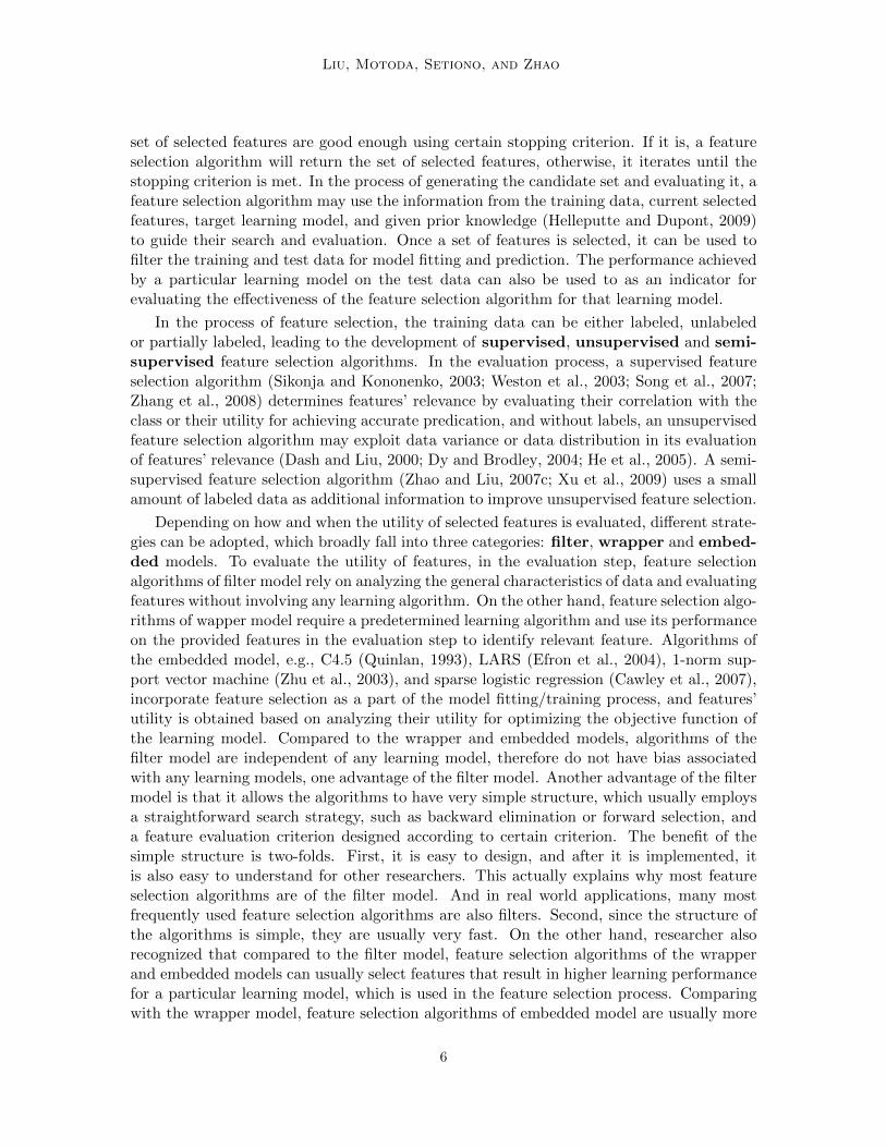
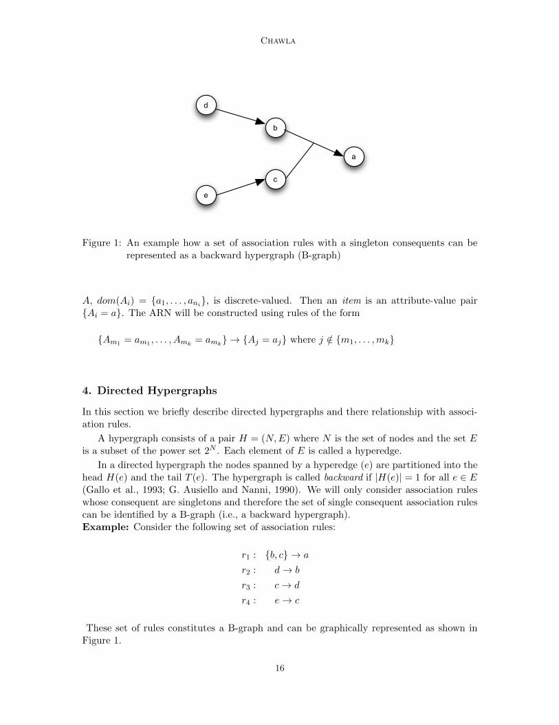
Figure 1: An example how a set of association rules with a singleton consequents can berepresented as a backward hypergraph (B-graph)
A, dom(Ai) = a1, . . . , ani, is discrete-valued. Then an item is an attribute-value pairAi = a. The ARN will be constructed using rules of the form
Am1 = am1 , . . . , Amk= amk
→ Aj = aj where j /∈ m1, . . . ,mk
4. Directed Hypergraphs
In this section we briefly describe directed hypergraphs and there relationship with associ-ation rules.
A hypergraph consists of a pair H = (N,E) where N is the set of nodes and the set Eis a subset of the power set 2N . Each element of E is called a hyperedge.
In a directed hypergraph the nodes spanned by a hyperedge (e) are partitioned into thehead H(e) and the tail T (e). The hypergraph is called backward if |H(e)| = 1 for all e ∈ E(Gallo et al., 1993; G. Ausiello and Nanni, 1990). We will only consider association ruleswhose consequent are singletons and therefore the set of single consequent association rulescan be identified by a B-graph (i.e., a backward hypergraph).Example: Consider the following set of association rules:
r1 : b, c → a
r2 : d→ b
r3 : c→ d
r4 : e→ c
These set of rules constitutes a B-graph and can be graphically represented as shown inFigure 1.
16

Feature Selection, Association Rules Network and Theory Building
5. Association Rules Network
In this section we formally define an Association Rules Network(ARN). Details about theARN, the algorithm to generate them, ARN properties and examples are given in (Pandeyet al., 2009).
Definition 1 Given a set of association rules R and a frequent goal item z which appearsas singleton in a consequent of a rule r ∈ R. An association rule network, ARN(R, z), isa weighted B-graph such that
1. There is a hyperedge which corresponds to a rule r0 whose consequent is the singletonitem z.
2. Each hyperedge in ARN(R, z) corresponds to a rule in R whose consequent is a sin-gleton. The weight on the hyperedge is the confidence of the rule.
3. Any node p 6= z in the ARN is not reachable from z.
6. Association Rules Network Process
We can use ARN as a systematic tool for feature selection. The steps involved are:
1. Prepare the data for association rule mining. This entails transforming the datainto transactions where each transaction is an itemset. Data where variables arecontinuous-valued, will have to be discretized.
2. Select and appropriate support and confidence threshold and apply an association rulemining algorithm to generate the association rules. Note that ARNs are target drivenso only those association rules are of interest which are directly or indirectly relatedto the target node. An association rule algorithm can be customized to generate onlythe relevant rules. Selecting the right support and confidence threshold is non-trivial.However, since our objective is to model the norm (rather than the exception), highervalues of the threshold are perhaps more suitable.
3. Build the Association Rule Network. Details are provided in (Pandey et al., 2009).This step has several exceptions which need to be handled systematically. For exam-ple, what happens if for the given support and confidence there is no association rulegenerated with the target node as the consequent? In which case either the support orthe confidence threshold or both have to be lowered. We may also choose to select thetop-k rules (by confidence) for the given target node. The advantage here is that wedon’t have to specify the confidence (or sometimes even the support) but now we haveto specify the “top-k.” Another advantage is generally we can also use the “top-k”approach to find rules in higher levels of the ARN.
4. Apply a clustering algorithm on the ARN to extract the relevant features (in thecontext of the target domain). The ARN is essentially a directed hypergraph. Theintuition is that first level nodes have an immediate effect on the target node whilehigher level nodes have an indirect influence. We can use a hypergraph clusteringalgorithm as illustrated in (Han et al., 1997).
17
Chawla
Data Association RulesAssociation Rules
Network
Hypergraph Clustering
FeaturesGood Fit Statistical Model
Implementation
Yes
No
Select Target Item
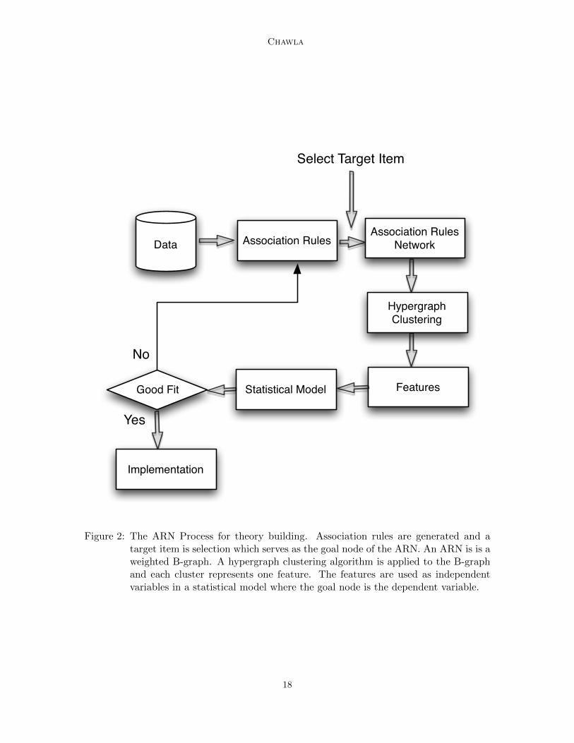
Figure 2: The ARN Process for theory building. Association rules are generated and atarget item is selection which serves as the goal node of the ARN. An ARN is is aweighted B-graph. A hypergraph clustering algorithm is applied to the B-graphand each cluster represents one feature. The features are used as independentvariables in a statistical model where the goal node is the dependent variable.
18

Feature Selection, Association Rules Network and Theory Building
spectacle prescription = myope
contact-lenses = hard
astigmatic = yes tear-prod-rate = normal age = young
(a) ARN for contact lens data with the target node as hard
tear-prod-rate = normalspectacle prescription = hypermetrope age = pre-prebyopicastigmatism = no
contact-lenses = soft
(b) ARN for contact lens data with target node as soft
Figure 3: ARN for the Contact Lens data. Clearly tear production rate does not seem likea good feature
5. The elements of the cluster are a collection of items (features) which are correlated.Choose one element of the cluster as the candidate feature. The number of clustersselected is a parameter and will require carefully calibration.
6. Build and test a statistical model (e.g., regression) to formally test the relationshipbetween the dependent and the candidate variables.
7. ARN Examples
We give two examples of ARN and show how they can be used for feature selection.
7.1 Contact Lens Example
We use a relatively simple data set from the UCI archive (Blake and Merz, 1998) to illustratehow ARNs can be used for feature selection. The ARN for the Lenses data are shown inFigure 3. The dependent variable is whether a patient should be fitted with hard contactlenses, soft contact lenses or should not be fitted with contact lenses. There are fourattributes. We built an ARN where the goal attribute is the class. Support and confidencewas chosen as zero. It is clear that both ARNs (for hard and soft lenses) can be used toelicit features which are important to distiguish between the two classes.
7.2 Open Source Software Example
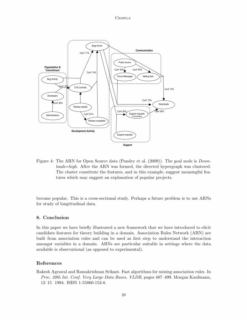
We have carried out an extensive analysis of the Open Source Software domain using ARN.Details can be obtained from (S.Chawla et al., 2003; Pandey et al., 2009). The OSS datawas obtained to understand why certain software products available from sourceforge.net
19
Chawla
Patches completed
Bug Activity
Developers
Administrators
CVS commits
Patches started
Public forums
Bugs found
Forum Messages Mailing lists
Downloads
Support requests Completed
Support requests
Conf: 71%
Conf: 72%
Conf: 85%
Conf: 81%
Conf: 74%
Conf: 80% Conf: 68%
Conf: 70%
Conf: 74%
Conf: 63% Conf: 55%
Organization & Commitment
Development Activity
Communication
Support
Figure 4: The ARN for Open Source data (Pandey et al. (2009)). The goal node is Down-loads=high. After the ARN was formed, the directed hypergraph was clustered.The cluster constitute the features, and in this example, suggest meaningful fea-tures which may suggest an explanation of popular projects.
become popular. This is a cross-sectional study. Perhaps a future problem is to use ARNsfor study of longtitudinal data.
8. Conclusion
In this paper we have briefly illustrated a new framework that we have introduced to elicitcandidate features for theory building in a domain. Association Rules Network (ARN) arebuilt from association rules and can be used as first step to understand the interactionamongst variables in a domain. ARNs are particular suitable in settings where the dataavailable is observational (as opposed to experimental).
References
Rakesh Agrawal and Ramakrishnan Srikant. Fast algorithms for mining association rules. InProc. 20th Int. Conf. Very Large Data Bases, VLDB, pages 487–499. Morgan Kaufmann,12–15 1994. ISBN 1-55860-153-8.
20
Feature Selection, Association Rules Network and Theory Building
C.L. Blake and C.J. Merz. UCI repository of machine learning databases, 1998. URLhttp://www.ics.uci.edu/∼mlearn/MLRepository.html.
G.F. Italiano G. Ausiello and U. Nanni. Dynamic maintenance of directed hypergraphs.Theoretical Computer Science, 72(2-3):97–117, 1990.
Giorgio Gallo, Giustino Longo, and Stefano Pallottino. Directed hypergraphs and applica-tions. Discrete Applied Mathematics, 42(2):177–201, 1993.
Eui-Hong Han, George Karypis, Vipin Kumar, and Bamshad Mobasher. Clustering basedon association rule hypergraphs. In Proceedings SIGMOD Workshop Research Issues onData Mining and Knowledge Discovery(DMKD ’97), 1997.
G. Pandey, S. Chawla, S. Poon, B. Arunasalam, and J. Davis. Association rules network:Definition and applications. Statistical Analysis and Data Mining, 1(4):260–279, 2009.
S.Chawla, B.Arunasalam, and J. Davis. Mining open source software(oss) data using as-sociation rules network. In Advances in Knowledge Discovery and Data Mining, 7thPacific-Asia Conference, PAKDD’03, pages 461–466. Springer, 2003.
21
JMLR: Workshop and Conference Proceedings 10: 22-34 The Fourth Workshop on Feature Selection in Data Mining
A Statistical Implicative Analysis Based Algorithm andMMPC Algorithm for Detecting Multiple Dependencies
Elham Salehi [email protected]
Jayashree Nyayachavadi [email protected]
Robin Gras [email protected]
department of Computer Science
University of Windsor
Windsor, Ontario, N9B 3P4
Editor: Huan Liu, Hiroshi Motoda, Rudy Setiono, and Zheng Zhao
Abstract
Discovering the dependencies among the variables of a domain from examples is an impor-tant problem in optimization. Many methods have been proposed for this purpose, but fewlarge-scale evaluations were conducted. Most of these methods are based on measurementsof conditional probability. The statistical implicative analysis offers another perspective ofdependencies. It is important to compare the results obtained using this approach withone of the best methods currently available for this task: the MMPC heuristic. As the SIAis not used directly to address this problem, we designed an extension of it for our purpose.We conducted a large number of experiments by varying parameters such as the number ofdependencies, the number of variables involved or the type of their distribution to comparethe two approaches. The results show strong complementarities of the two methods.
Keywords: Statistical Implicative Analysis, multiple dependencies, Bayesian network.
1. Introduction
There are many situations in which finding the dependencies among the variables of a do-main is needed. Therefore having a model describing these dependencies provides significantinformation. For example, which variable(s) affect(s) the other variable(s) may be very use-ful for the problem of selection of variables; decomposition of a problem to independentsub-problems; predicting the value of a variable depending on other variables to solve theclassification problem; finding an instantiation of a set of variables for maximizing the valueof some function, etc (A. Goldebberg, 2004; Y. Zeng, 2008).
The classical model used for the detection of dependencies is the Bayesian network.This network is a factorization of the probability distribution of a set of examples. It is wellknown that the construction of a Bayesian network from examples is a NP-hard problem,thus different heuristic algorithms have been designed to to solve this problem (Neapolitan,2003; E. Saheli, 2009) . Most of these heuristics are greedy and/or try to reduce the size ofthe exponential search space by a filtering strategy. The filtering is based on some measuresthat aim to discover sets of variables that have high potentiality to be mutually dependentor independent.
c©2010 Salehi, Nyayachavadi and Gras.
Detecting Multiple Dependencies
These measures rely on an evaluation of the degree of conditional independency. How-ever other measures exist which are not based on conditional probability measurements thathave the ability to discover dependencies. Using another measure that is not based on con-ditional dependencies can provide another perspective about the structure of dependenciesof variables of a domain. Statistical Implicative Analysis (SIA) has already shown a greatcapability in extracting quasi-implications also called as association rules (R. Gras, 2008).We present a measure for multiple dependencies based on SIA and then use this measurein a greedy algorithm for solving the problem of multiple dependencies detection. We havecompared our new algorithm for finding dependencies with one of the most successful con-ditional dependencies based heuristic introduced so far, MMPC (I. Tsamardinos, 2006). Wehave designed a set of experiments to evaluate the capacity of each of them to discover twokinds of knowledge: the fact that one variable conditionally depends on another one andthe sets of variables that are involved in a conditional dependencies relation. Both of thisinformation can be used to decompose the NP-hard problem of finding the structure of aBayesian network into independent sub-problems and therefore can reduce considerably thesize of corresponding search space.
This paper organized as follows: In the next section we describe the MMPC heuristic. Insection 3 we present our SIA based measure and algorithm for finding multiple dependenciesand the experimental results of the algorithms are presented in Section 4. Finally weconclude in section 5 with a brief discussion.
2. The MMHC Heuristic
Discovering multiple dependencies from a set of examples is a difficult problem. It is clearthat this problem cannot be solved exactly when the number of variables approaches fewdozens . However, for some problems, the number of variables can be several hundred orseveral thousand. Therefore, it is particularly important to have some methods to obtainan approximate solution with good quality. A local search approach is usually used inthese problems. In this case the model of dependencies is built incrementally by addingor removing one or more dependencies at each step. The dependencies are chosen to beadded or removed using a score that assesses the quality of the new model according tothe set of examples (E. Saheli, 2009). In this approach the search space is exponential interms of maximum number of variables on which a variable may depend. Therefore, thereis a need to develop methods to increase the chances of building a good quality modelwithout exploring the whole search space exhaustively. One possible approach is to use aless computationally expensive method to determine a promising subset of the search spaceon which we can subsequently apply a more systematic and costly method.
The final model is usually a Bayesian network in which the dependencies represent con-ditional independencies among variables. It is possible to build this model using informationfrom other measures besides conditional probability. Indeed, the measurements in the firstphase are used as a filter to eliminate the independent variables or bring the variables withshared dependencies together in several sub-groups. The second phase uses this filteredinformation to build a Bayesian network. The goal of our study is to compare the abilityof two approaches for the detection of dependencies for the first phase. In this section a
23

Salehi, Nyayachavadi and Gras
measure based on conditional probability is described and in the section 4 this measure willbe compared with a SIA based measure.
2.1 Definition and Notation
A Bayesian network is a tool to represent the joint distribution of a set of random variables.Dependency properties of this distribution are coded as a direct acyclic graph (DAG).The nodes of this graph are random variables and the arcs correspond to direct influencesbetween the variables.
We consider a problem consisting of n variables v1, v2, . . . , vn. Each variable vi can takeany values in setMi = mi,1,mi,2, . . . ,mi,k. For the detection of dependencies a set of Nexamples is available. Each example is an instantiation of each of the n variables in one ofk possible ways.
Pari, the set of all variables on which variablevi depends, is the parent set of vi .Anyvj ∈ Pari is a parent of vi and vi is a child of vj . A table of conditional probabilitydistribution (CPD), also known as the local parameters, is associated for each node of thegraph. This table represents the probability distribution P (vi|Pari).
2.2 MMPC Approach
Although learning Bayesian networks might seem a very well-researched area and even someexact algorithms have been introduced for networks with less than 30 variables (M. Koivisto,2004), applying them to many domains such as biological or social networks, faces theproblem of high dimensionality. In recent years several algorithms have been devised tosolve this problem by restricting the space of possible network structures using variousheuristics (N. Friedman, 1999; I. Tsamardinos, 2006). One of these algorithms, which has apolynomial complexity is ”Sparse Candidate” algorithm (N. Friedman, 1999). The principleof this method is to restrict the parent set of each variable assuming that if two variablesare almost independent in the set of examples, it is very unlikely that they are connected inthe Bayesian network. Thus, the algorithm builds a small fixed-size candidate parent set foreach variable. A major problem of this algorithm is to define the size of the possible parentsets and another one is that the algorithm assumes a uniform sparseness in the network.More recently, another algorithm called Max-Min Hill Climber (MMHC) has been proposedto solve these two problems and obtain better results on a wider range of network structures(I. Tsamardinos, 2006).This algorithm, uses a constrained based method to discover possibleparents-children relationships and then uses them to build a Bayesian network. The firststep of this algorithm, the one we use in this section to detect dependencies, is calledMax-Min Parent Children (MMPC). The MMPC algorithm uses a data structure calledparent-children set, for each variable vi that contains all variables that are a parent or achild of vi in any Bayesian network faithfully representing the distribution of the set ofexamples. The definition of faithfulness can be found in (Neapolitan, 2003; I. Tsamardinos,2006). MMPC uses G2 statistical test (P. Spirtes, 2000) on the set of examples to determinethe conditional independency between pairs of variables given a set of other variables. TheMMPC algorithm consists of two phases. In the first phase, an empty set of candidateparents-children (CPC) is associated with vi. Then it tries to add more nodes one by oneto this set using MMPC heuristic. This heuristic selects the variable vj that maximizes
24
Detecting Multiple Dependencies
the minimum association with vi relative to current CPC and add this variable to it. Theminimum association of vj and vi relative to a set of variables CPC is defined as below.
MinAssoc(vi; vj |CPC) = argminAssoc(vi; vj |S) for all subset S of CPC.
Assoc (vi, vj |S) is an estimate of the strength of the association between vi and vjknowing the CPC and is equal to zero if vi and vj are conditionally independent given theCPC. The function Assoc uses the p-value returned by the G2 test of independence: thesmaller the p-value the higher the association. The first phase of MMPC stops when allremaining variables are considered independent of vi given the subset of CPC. This approachis greedy, because a variable added in one step of this first phase may be unnecessary afterother variables were added to the CPC. The second phase of MMPC tries to fix this problemby removing those variables in CPC which are independent of vi given a subset of the CPC.Since this algorithm looks for candidate parents-children set for each node, if node T is inCPC of node X, node X should also be in CPC of node T .
What is not clear about these methods are their capabilities to discover any kind ofstructures and how different conditional probabilities and structures of real networks influ-ence on the quality of results. We present the result we have obtained using the MMPCalgorithm on examples generated from various Bayesian networks in Section 4.
3. SIA Based Approach
Statistical Implicative Analysis (SIA) (R. Gras, 2008) is a data analysis method that offersa framework for extracting quasi-implications also called as association rules. In a datasetD of N instances, each instance being a set of n Boolean variables, the implicative intensitymeasures to what extent variable b is true if variable a is true. The quality measure usedin SIA is based on the unlikelihood of counter-examples where b is false and a is true.We are interested in the capabilities of SIA for finding multiple dependencies especially insituations that are difficult for conventional methods that are based on other measurements.For example, a situation in which two variables are independent but often take the samevalue in a large number of examples. We want to study the efficiency of SIA to refute thehypothesis of dependence by taking into account the counter examples. In order to usethe SIA in general, some modifications are necessary. Indeed, we do not restrict ourselvesto the binary variables and generalize the method for variables with higher cardinalities.We also want to be able to detect a situation where a combination of variables impliesanother variable, using an overall measure. In other word we want to measure one or morecombinations of variables as the parents of a child variable. For example for variables A,B and C ∈ 0, 1, 2, we want to define a measure which is able to detect a dependencyfrom B and C to A because when B = 0 ∧ C = 2, A = 1 is abnormally frequent and whenB = 0 ∧ C = 0, A = 0 is abnormally frequent. Current version of the SIA cannot be usedfor this purpose.
3.1 Definition and Notation
We use the following definitions and notations besides those presented in section 2.1. Allthe definitions presented here and the proofs for the rational of the measures and theirproperties can be found in (R. Gras, 2008). Let Card(mi,j) be the number of times the
25
Salehi, Nyayachavadi and Gras
variable vi takes the value mi,j in N examples. Card(mi,j) is the number of times thevariable vi takes a value different from mi,j and Card(mi1,j1 ,mi2,j2) the number of timesthe variable vi1 takes the value mi1,j1 and variable vi2 takes value mi2,j2 in N examples.
Let πi be an instantiation of the parents of vi chosen from Πi, the list of all combinationsof instantiation of vi parents. For example, in the previous example with the variables A,B and C, ΠA = (0, 0), (0, 1), (0, 2), (1, 0), (1, 1), (1, 2), (2, 0), (2, 1), (2, 2). If k = |Mi| thenfor each vj ∈ Pari
|Πi| = k|Pari|.
Let Card(πi) be the number of times all parents of vi, take value πi in the N examples.Then the measure q extended from SIA is
q(πi,mi,j) =Card(πi∧mi,j)−
Card(πi)×Card(mi,j)N√
Card(πi)×Card(mi,j)N
.
And the inclusion index i(πi,mi,j) for measuring the imbalances is extended from SIA is
i(πi,mi,j) = (Iαmi,j/πi .Iαmi,j/πi
)1/2α.
If we define function f as belowf(a, b) = Card(a∧b)
card(a)Then
Iαmi,j/πi = 1 + ((1− f(πi,mi,j)) log2((1− f(πi,mi,j)) + f(πi,mi,j) log2((f(πi,mi,j)).
If Card(πi ∧mi,j ∈ [0, Card(πi2 [; otherwise, Iαmi,j/πi = 0; and
Iαπi/mi,j = 1 + ((1− f(mi,j , πi)) log2((1− f(mi,j , πi)) + f(mi,j , πi) log2((f(mi,j , πi)).
In above equations α = 1.The score we try to maximize is
s(πi,mi,j) = −i(πi,mi,j)× q(πi,mi,j).
3.2 Extension of SIA
Unfortunately, the current SIA measure considers only one instantiation of the parent setat a time. If we want to consider all possible instantiations of the parent set we willobtain as many different dependency measures as there are different possible combinationof instantiation. However, for each variable vi, we need a single measure that represents itsdegree of dependency with its parent set. Therefore we must consider all the combinationof variables for Πi and use the measures s(πi,mi,j), to see how they imply all the possiblevalues of vi. Consequently we build a table Ti containing the set Πsi of measures s for allthe combination of Πi and Mi with size
k × |πi| = k|par(vi)|.
We tried various methods to combine the information of this table to a single measure. Thesimplest way is to consider just the maximum of Πsi. Other possibilities are to take theaverage of Πsi or the average of the x% of highest scores. We conducted many test withthese approaches and none of them has yielded satisfactory results. In the first series ofmeasures we considered the scores of one instantiation of πi , but different values of Mi
26

Detecting Multiple Dependencies
B C A= 0 A =1 A =2 Sup E
0 0 0 1.3 0.6 1.3 0.2720 1 0 0 0 0 00 2 2.1 0 0.2 2.1 0.1291 0 0 0 0 0 01 1 0.4 0.2 0.5 0.5 0.451 2 1.1 0 0 1.1 02 0 0 0 0 0 02 1 0 0 0 0 02 2 0 0 0 0 0
Table 1: An example of table Ti with A,B and C ∈ 0, 1, 2and A=(0, 0), (0, 1), (0, 2), (1, 0), (1, 1),(1, 2), (2, 0), (2, 1), (2, 2).
independently. What we want to detect is that a value of πi imply one specific instantiationof vi and we want that it is true for several different instantiations of πi. Therefore ameasure is needed to detect that s is high for a couple (πi,mi,j) with mi,j ∈ Mi and lowfor all the others mi,j ∈ Mi and that it is true for several πi. We have therefore defined ascore which combine, for a given πi, the maximum value Supπi of s for all mi,j ∈ Mi andthe entropy Eπi of s for all the values mi,j ∈Mi.
Supπi = max(s(πi,mi,j)) where 1 ≤ j ≤ k,
Eπi = −k∑
j=1
p(s(πi,mi,j)) log(p(s(πi,mi,j))
log(k)
where
p(s(πi,mi,j)) =s(πi,mi,j)
k∑
j=1
s(πi,mi,j)
.
For calculating a measure associated with a table Ti, we consider a set H of those πicorresponding to the highest x% of Supπi values in the table. Then the score of the table is
Si,Pari =
∑
πi∈HSupπi
∑
πi∈HEπi
.
This is the measure we want to maximize. Table 1 presents TA for the example withvariables A,B,C. If you select the highest 20% Sup, only lines 1 and 3 will be selectedand SA will be equal to 8.48. In the following section we give an algorithm that uses thismeasure to determine the major dependencies of a problem.
3.3 SIA Based Algorithm
In previous section we defined a measure Si for each variable vi knowing its parent set. Todetermine the dependencies of a problem we should consider different possible configurationsof parent sets for all variables and choose the configuration that leads to a maximum total
27
Salehi, Nyayachavadi and Gras
score. Since the number of possible configurations is exponential in the number of variables,we need a heuristic approach. We chose an greedy approach for this heuristic. In thebeginning of the algorithm we set the parent set of each variable to empty. Then at eachstep a new variable is chosen to be added to any of the parent sets using measure S. We stopadding variables when a fixed number of edges, maxEdge, has been added. The calculationof the table Ti is also exponential in the number of parents of variables so we restrict themaximum number of parents for each variable to four.The next variable to be added to aparent set is chosen by comparing the highest score of four different tables. The algorithm ispresented in Table 2. This algorithm avoids calculating the score for all combinations of 2,3 and 4 variables in a parent set. Only combinations that include x parents can be selectedto calculate the score with x + 1 parents. The variable structMax includes: the score ofthe variable regarding its parent set, the child variable and the candidate parent variableto be added to the parent set. After initialization, table max1 contains a list of the scoresin descending order of all the combinations including one parent and one child. So there isn2 scores in it. Tables max2, max3 and max4 are initially empty. They are used to storethe scores of child-parents combination when there are 2, 3 and 4 parents in the parent setsrespectively. Thus at each stage of the algorithm, the variable to be added to the parent setof another variable will be determined by selecting the highest score of 4 tables. If Maxiis the selected table, the parent set of the variable associated with the maximum score forthis table goes from i-1 to i variables. The score is then removed from the table and a newmax score is calculated and inserted in the table maxi+1.The four tables are kept sorted indescending order so the maximum value of each table is always in position 0.
4. Experimental Study
In this section we study the capabilities of the MMPC heuristics and our SIA algorithmin finding the conditional dependencies and dependent variables involved in conditionaldependencies.
4.1 Experimental Design
In our experiments, we use artificial data produced by sampling from randomly generatedBayesian networks. Each network has A arcs and n = 100 variables divided into two sets:a set of D variables for which there are direct dependency relations with at least one of then-D-1 other variables; a set of variables I with no dependency relationship with any of theother n-1 variables. The CPD of each variable is randomly generated taking into accountthe possible dependency relations. Each variable can take 3 different values.
We represent the distribution of independent variables as a triplet such (p1,p2, p3). Forexample (80, 10, 10) means that each random variable has a probability of 0.8 for oneof its three possible values, and a probability of 0.1 for the other two. The value with aprobability of 0.8 is chosen randomly among the three random variables. For distributionscalled ’random’, each variable has a different distribution (p1,p2, p3).
28

Detecting Multiple Dependencies
for all ViPari = ∅
structMax = 0, 0, 0max1 = ∅for sall Vi
for all vj 6= viif (Si,Pari+vi > structMax.score) sturctMax.score = Si,Pari+vi
structMax.child = istructMax.parent = j
max1 = max1 + structMax
DescendingSort (maxi)max2 = ∅,max3 = ∅,max4 = ∅nbEdge = 0while (nbEdge < maxEdge) k = getIndexOfTableWithMaxScore(max1,max2,max3,max4)enf = maxk[0].childparchild = parchild +maxk[0].parentif (k < 4) structMax = 0, 0, 0for all vj /∈ parchild if (Si,Pari+vi > structMax.score) sturctMax.score = Si,Pari+vistructMax.child = istructMax.parent = jmaxk+1 = maxk+1 + structMaxDescendingSort (maxk+1)maxk[0] = 0, 0 ,0 DescendingSort (maxk)nbEdge = nbEdge+ 1
Table 2: SIA based Algorithm.
4.2 Evaluation of MMPC Heuristic
In this section, we study the ability of the MMPC algorithm to discover good parent-childsets of variables from data generated from Bayesian networks.
In our study, we vary the characteristics of the networks to analyze the consequencesof this variation on the effectiveness of the MMPC algorithm. These changes include thedistribution of independent variables I, the number of dependent variables D and the numberof dependencies among the variables D (i.e. the number of arcs A in the network). Theresults are presented in Tables 3 to 4. Each row of these tables represents an average ofresults for 10 different sets of examples generated from 10 different networks but with thesame characteristics. In each experiment, we calculate the mean and standard deviationof the number of true positive (TP), False Positives (FP), False Negative (FN) and thecomputational time. TP is the number of parent-children relationships correctly predictedby the algorithm. Thus, the number of TP at most can be twice the number of arcs ofthe network because if there is an arc between node X and node T it means each of them
29
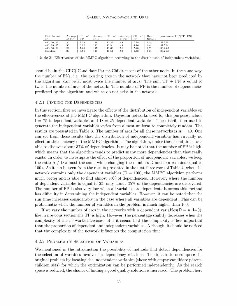
Salehi, Nyayachavadi and Gras
Distributionof I
Averageof TP
SD ofTP
Averageof FP
SD ofFP
Averageof FN
SD ofFN
Runtimes(S)
precision= TP/(TP+FN)
(80, 10, 10) 30 7.29 116 11.33 49 7.28 6.5 37.5%(50, 25, 25) 30 8.12 113 11.9 49 8.16 6.4 37.5%(40, 30, 30) 29 7.28 117 11.63 51 7.28 6.7 36.25%Random 29 6.76 118 10.54 50 6.78 6.2 36.25%
Table 3: Effectiveness of the MMPC algorithm according to the distribution of independent variables.
should be in the CPC( Candidate Parent-Children set) of the other node. In the same way,the number of FNs, i.e. the existing arcs in the network that have not been predicted bythe algorithm, can be at most twice the number of arcs. The sum TP + FN is equal totwice the number of arcs of the network. The number of FP is the number of dependenciespredicted by the algorithm and which do not exist in the network.
4.2.1 Finding the Dependencies
In this section, first we investigate the effects of the distribution of independent variables onthe effectiveness of the MMPC algorithm. Bayesian networks used for this purpose includeI = 75 independent variables and D = 25 dependent variables. The distribution used togenerate the independent variables varies from almost uniform to completely random. Theresults are presented in Table 3. The number of arcs for all these networks is A = 40. Onecan see from these results that the distribution of independent variables has virtually noeffect on the efficiency of the MMPC algorithm. The algorithm, under these conditions, wasable to discover about 37% of dependencies. It may be noted that the number of FP is high,which means that the algorithm tends to predict many more dependencies than that reallyexists. In order to investigate the effect of the proportion of independent variables, we keepthe ratio A / D almost the same while changing the numbers D and I (n remains equal to100). As it can be seen from the results presented in the first three rows of Table 4, when thenetwork contains only the dependent variables (D = 100), the MMPC algorithm performsmuch better and is able to find almost 80% of dependencies. However, where the numberof dependent variables is equal to 25, only about 35% of the dependencies are discovered.The number of FP is also very low when all variables are dependent. It seems this methodhas difficulty in determining the independent variables. However, it can be noted that therun time increases considerably in the case where all variables are dependent. This can beproblematic when the number of variables in the problem is much higher than 100.
If we vary the number of arcs in the networks with n dependent variables(D = n, I=0),like in previous section,the TP is high. However, the percentage slightly decreases when thecomplexity of the networks increases. But it seems that the complexity is less importantthan the proportion of dependent and independent variables. Although, it should be noticedthat the complexity of the network influences the computation time.
4.2.2 Problem of Selection of Variables
We mentioned in the introduction the possibility of methods that detect dependencies forthe selection of variables involved in dependency relations. The idea is to decompose theoriginal problem by locating the independent variables (those with empty candidate parent-children sets) for which the optimization can be performed independently. As the searchspace is reduced, the chance of finding a good quality solution is increased. The problem here
30

Detecting Multiple Dependencies
D I A Averageof TP
SD ofTP
Averageof FP
SD ofFP
Averageof FN
SD ofFN
Run times (s) precision= TP/(TP+FN)
25 75 40 29 6.76 118 10.54 50 6.78 0.31 36.250 50 80 53.4 8.81 99.4 11.35 106.6 8.81 0.34 33.4100 0 150 243.8 8.17 16.6 6.81 56.2 8.17 21.1 81.325 0 30 52.4 3.55 2.4 1.96 7.6 3.55 0.31 87.325 0 40 65.6 4.17 2.2 1.89 14.4 4.17 1.83 8225 0 60 91.8 4.51 3.2 3.37 28.2 4.51 6.63 76.5100 0 120 200.6 5.51 25.2 7.28 39.4 5.52 9.98 83.6100 0 150 243.8 8.17 16.6 6.81 56.2 8.17 21.1 81.3100 0 200 312.4 9.67 10.8 3.37 87.6 9.67 28.3 78.1
Table 4: The average efficiency of MMPC algorithm regarding the proportion of independent variables andcomplexity of the Bayesian network.
Distribution D A TP TN
random 25 60 24.2 11.4random 25 40 23.2 12.4random 25 30 24 10.6(80, 10, 10) 25 40 23.8 12.6(50, 25, 25) 25 40 23.8 13.6(40, 30, 30) 25 40 23.8 13.8
Table 5: Results obtained by the MMPC algorithm for the problem of selection of variables.
is slightly easier than the one studied in section 4.2.1 because the goal here is to determinethe list of variables involved in dependency relationships without finding the dependenciesprecisely. We therefore conducted a series of experiments to measure the capacity of theMMPC on this problem.
We used networks with different independent variable distributions generated using themethod described in section 4.1. We also vary the complexity of the networks by changingthe number of arcs. The results are presented in Table 5. Although the MMPC approachcould discover more than 90% of the dependent variables in Table 5 (23 out of 25), itdiscovered just about 17% of independent variables (TN in Table 5). This means that thismethod tends to significantly overestimate the number of dependencies. The results arelittle affected by changing distributions of independent variables and the complexity of thenetwork (results not shown). It seems that this method cannot be used for the problem ofselection of variables because almost all variables are selected.
4.3 Evaluation of SIA Based Algorithm
We repeated the same experiences as those in Section 4.2 to evaluate our SIA based detectionalgorithm in order to achieve the most possible honest comparison. It should be notedthough that this disadvantaged SIA. Indeed, the data were generated from the models,Bayesian networks, which are based on conditional probability measurement. The SIAapproach uses an alternative measure that does not have the same properties. In particular,a very significant difference is that the Bayesian network model is not transitive whilethe SIA is. But a totally fair comparison is not possible and, taking into account thesedifferences in our analysis, this comparison seemed to be the best way to proceed.
31
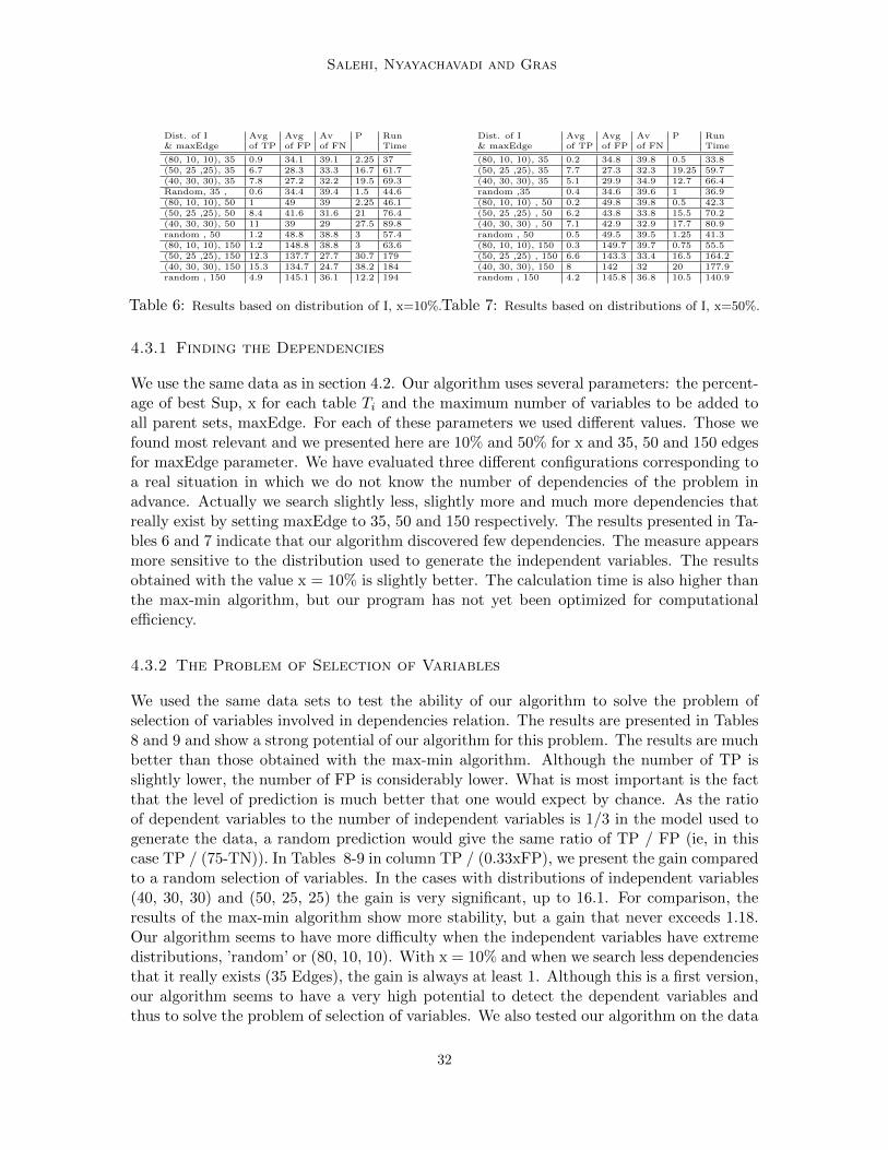
Salehi, Nyayachavadi and Gras
Dist. of I Avg Avg Av P Run& maxEdge of TP of FP of FN Time
(80, 10, 10), 35 0.9 34.1 39.1 2.25 37(50, 25 ,25), 35 6.7 28.3 33.3 16.7 61.7(40, 30, 30), 35 7.8 27.2 32.2 19.5 69.3Random, 35 , 0.6 34.4 39.4 1.5 44.6(80, 10, 10), 50 1 49 39 2.25 46.1(50, 25 ,25), 50 8.4 41.6 31.6 21 76.4(40, 30, 30), 50 11 39 29 27.5 89.8random , 50 1.2 48.8 38.8 3 57.4(80, 10, 10), 150 1.2 148.8 38.8 3 63.6(50, 25 ,25), 150 12.3 137.7 27.7 30.7 179(40, 30, 30), 150 15.3 134.7 24.7 38.2 184random , 150 4.9 145.1 36.1 12.2 194
Table 6: Results based on distribution of I, x=10%.
Dist. of I Avg Avg Av P Run& maxEdge of TP of FP of FN Time
(80, 10, 10), 35 0.2 34.8 39.8 0.5 33.8(50, 25 ,25), 35 7.7 27.3 32.3 19.25 59.7(40, 30, 30), 35 5.1 29.9 34.9 12.7 66.4random ,35 0.4 34.6 39.6 1 36.9(80, 10, 10) , 50 0.2 49.8 39.8 0.5 42.3(50, 25 ,25) , 50 6.2 43.8 33.8 15.5 70.2(40, 30, 30) , 50 7.1 42.9 32.9 17.7 80.9random , 50 0.5 49.5 39.5 1.25 41.3(80, 10, 10), 150 0.3 149.7 39.7 0.75 55.5(50, 25 ,25) , 150 6.6 143.3 33.4 16.5 164.2(40, 30, 30), 150 8 142 32 20 177.9random , 150 4.2 145.8 36.8 10.5 140.9
Table 7: Results based on distributions of I, x=50%.
4.3.1 Finding the Dependencies
We use the same data as in section 4.2. Our algorithm uses several parameters: the percent-age of best Sup, x for each table Ti and the maximum number of variables to be added toall parent sets, maxEdge. For each of these parameters we used different values. Those wefound most relevant and we presented here are 10% and 50% for x and 35, 50 and 150 edgesfor maxEdge parameter. We have evaluated three different configurations corresponding toa real situation in which we do not know the number of dependencies of the problem inadvance. Actually we search slightly less, slightly more and much more dependencies thatreally exist by setting maxEdge to 35, 50 and 150 respectively. The results presented in Ta-bles 6 and 7 indicate that our algorithm discovered few dependencies. The measure appearsmore sensitive to the distribution used to generate the independent variables. The resultsobtained with the value x = 10% is slightly better. The calculation time is also higher thanthe max-min algorithm, but our program has not yet been optimized for computationalefficiency.
4.3.2 The Problem of Selection of Variables
We used the same data sets to test the ability of our algorithm to solve the problem ofselection of variables involved in dependencies relation. The results are presented in Tables8 and 9 and show a strong potential of our algorithm for this problem. The results are muchbetter than those obtained with the max-min algorithm. Although the number of TP isslightly lower, the number of FP is considerably lower. What is most important is the factthat the level of prediction is much better that one would expect by chance. As the ratioof dependent variables to the number of independent variables is 1/3 in the model used togenerate the data, a random prediction would give the same ratio of TP / FP (ie, in thiscase TP / (75-TN)). In Tables 8-9 in column TP / (0.33xFP), we present the gain comparedto a random selection of variables. In the cases with distributions of independent variables(40, 30, 30) and (50, 25, 25) the gain is very significant, up to 16.1. For comparison, theresults of the max-min algorithm show more stability, but a gain that never exceeds 1.18.Our algorithm seems to have more difficulty when the independent variables have extremedistributions, ’random’ or (80, 10, 10). With x = 10% and when we search less dependenciesthat it really exists (35 Edges), the gain is always at least 1. Although this is a first version,our algorithm seems to have a very high potential to detect the dependent variables andthus to solve the problem of selection of variables. We also tested our algorithm on the data
32
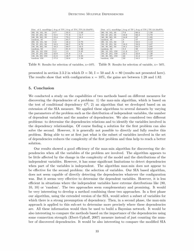
Detecting Multiple Dependencies
Dist. of I, maxEdge Avg of TP Avg of TN TP/(0.33xFP)
(80, 10, 10), 35 6.7 55.5 1.03(50, 25 ,25), 35 15.5 71.8 14.7(40, 30, 30), 35 15.4 72.1 16.1random, 35 3.4 64.7 1(80, 10, 10), 50 6.8 46.4 0.73(50, 25 ,25), 50 18.3 68.7 8.79(40, 30, 30), 50 18.3 69.7 10.5random, 50 6.1 61.3 1.36(80, 10, 10) 150 9.2 13 0.45(50, 25 ,25) 150 22.8 31.8 1.6(40, 30, 30) 150 21.8 46.7 2.33random 150 17.3 32.6 1.24
Table 8: Results for selection of variables, x=10%.
Dist. of I, maxEdge Avg of TP Avg of TN TP/(0.33xFP)
(80, 10, 10), 35 7.6 60.4 1.58(50, 25 ,25), 35 16.8 66.2 5.79(40, 30, 30), 35 14.8 67 1.85random, 35 4 57 0.67(80, 10, 10), 50 8 53.5 1.13(50, 25 ,25), 50 18.3 59.9 3.67(40, 30, 30), 50 18.1 63.7 4.85random, 50 5.5 50 0.67(80, 10, 10), 150 11.8 6.7 0.52(50, 25 ,25), 150 22.1 22.8 1.28(40, 30, 30), 150 22 41.2 1.97random, 150 22 16.5 1.14
Table 9: Results for selection of variable, x= 50%.
presented in section 2.3.2 in which D = 50, I = 50 and A = 80 (results not presented here).The results show that with configuration x = 10%, the gains are between 1.28 and 1.82.
5. Conclusion
We conducted a study on the capabilities of two methods based on different measures fordiscovering the dependencies of a problem: 1) the max-min algorithm, which is based onthe test of conditional dependency G2; 2) an algorithm that we developed based on anextension of the SIA measure. We applied these algorithms to several datasets by varyingthe parameters of the problem such as the distribution of independent variables, the numberof dependent variables and the number of dependencies. We also considered two differentproblems: to determine the dependencies relations and to identify the variables involved inthe dependency relationships. Of course finding a solution for the first problem can alsosolve the second. However, it is generally not possible to directly and fully resolve thisproblem. Being able to see at first just what is the subset of variables involved in the setof dependencies reduces the complexity of the first problem and thus help to reach a bettersolution.
Our results showed a good efficiency of the max-min algorithm for discovering the de-pendencies when all the variables of the problem are involved. The algorithm appears tobe little affected by the change in the complexity of the model and the distributions of theindependent variables. However, it has some significant limitations to detect dependencieswhen part of the variables is independent. The algorithm max-min does not appear tobe effective for the second problem: the selection of variables. Our SIA based algorithm,does not seem capable of directly detecting the dependencies whatever the configurationwas. But it seems very effective to determine the dependent variables. However, it is lessefficient in situations where the independent variables have extreme distributions like (80,10, 10) or ’random’. The two approaches seem complementary and promising. It wouldbe very interesting to develop a method combining these two approaches. In a first phaseour algorithm, using the extended version of the SIA, would select a subset of variables forwhich there is a strong presumption of dependency. Then, in a second phase, the max-minapproach is applied to this sub-set to determine more precisely where these dependenciesare. All these information would then be used to build a Bayesian network. It would bealso interesting to compare the methods based on the importance of the dependencies usingsome connection strength (Ebert-Uphoff, 2007) measure instead of just counting the num-ber of discovered dependencies. It would be also interesting to compare the modified SIA
33
Salehi, Nyayachavadi and Gras
with multi-dimensional form of classical measures to detect correlation between variabledistributions.
References
A. Moore A. Goldebberg. Tractable learning of large bayes net structures from sparse data.In 21th International Conference on Machine Learning, pages 44–51, 2004.
R. Gras E. Saheli. An empirical comparison of the efficiency of several local search heuristicsalgorithms for bayesian network structure learning. In Learning and Intelligent Optimiza-tion IEEE international conference, 2009.
I. Ebert-Uphoff. Measuring connection strenghts and link strenghts in discrete bayesiannetworks. Technical Report GT-IIC-07-01, Georgia Tech, College of Computing, January2007.
C.F. Aliferis I. Tsamardinos, L. E. Brown. The mmpc hill-climbing bayesian network struc-ture learning algorithm. Machine Learning Journal, 65(1):31–78, 2006.
K Sood M. Koivisto. Exact bayesian structure discovery in bayesian networks. Journal ofMachine Learning Research, 5:549–573, 2004.
D. Peer N. Friedman, I. Nachman. Learning bayes network structure from massive datasets:The ”sparse candidate” algorithm. In 15th Conference on Uncertainty in Artificial Intel-ligence, pages 206–215, 1999.
R. Neapolitan. Learning Bayesian networks. Prentice Hall, 2003.
R. Scheines P. Spirtes, C. Glymour. Causation, prediction, and search. The MIT Press,second Edition, 2000.
P Kuntz et al R. Gras. An overview of the Statistical Implicative. In: Statistical ImplicativeAnalysis. Springer-Verlag, 2008.
C.A. Hernandez Y. Zeng. Decomposition algorithm for learning bayesian network structuresfrom data. In PAKDD 2008, Lecture Notes in Artificial Intelligence, pages 441–453, 2008.
34
JMLR: Workshop and Conference Proceedings 10: 35-44 The Fourth Workshop on Feature Selection in Data Mining
Attribute Selection Based on FRiS-Compactness
Nikolai G. Zagoruiko [email protected] of Mathematics SD RAS, pr. Koptyg 4,Novosibirsk 630090, Russia
Irina A. Borisova [email protected] of Mathematics SD RAS, pr. Koptyg 4,Novosibirsk 630090, Russia
Vladimir V. Duybanov [email protected] State University Pirogov st. 2,Novosibirsk 630090, Russia
Olga A. Kutnenko [email protected]
Institute of Mathematics SD RAS, pr. Koptyg 4,
Novosibirsk 630090, Russia
Editor: Huan Liu, Hiroshi Motoda, Rudy Setiono, and Zheng Zhao
Abstract
Commonly to classify new object in Data Mining one should estimate its similarity withgiven classes. Function of Rival Similarity (FRiS) is assigned to calculate quantitative mea-sure of similarity considering a competitive situation. FRiS-function allows constructingnew effective algorithms for various Data Mining tasks solving. In particular, it enablesto obtain quantitative estimation of compactness of patterns which can be used as indi-rect criterion for informative attributes selection. FRiS-compactness predicts reliability ofrecognition of control sample more precisely, than such widespread methods as One-Leave-Out and Cross-Validation. Presented in the paper results of real genetic task solving confirmefficiency of FRiS-function using in attributes selection and decision rules construction.
Keywords: Pattern recognition, Function of Rival Similarity, Compactness, Iformative-ness
1. Introduction
Two main parts “engine” and “criterion” can be partitioned in attribute selection algo-rithms. Engine forms different variants of attributes subsystems and criterion estimatesquality of considered systems. We guess that the main element of the engine is algorithmof directed search, the main characteristic calculated by criterion is compactness of the pat-terns, and the basic element in compactness estimation is a measure of objects similarity.These three items are considered in this work. In Section 2 relative measure of similarity(FRiS-function) is introduced, measure of compactness of patterns based on FRiS-functionis defined in Section 3, in Section 4 algorithm for decision rule construction FRiS-Stolp is de-scribed. Then, in Section 5 algorithm FRiS-GRAD for simultaneous attribute selection anddecision rule construction is proposed. Effectiveness of this algorithm on real recognitiontask is illustrated in Section 6.
c⃝2010 Zagoruiko, Borisova, Duybanov and Kutnenko.
Zagoruiko, Borisova, Duybanov and Kutnenko
2. How to estimate similarity?
Similarity of two objects z and a according to some attribute X in metric space usuallydepeds on difference R(z, a) between values of X for these objects. Many such type measuresof similarity are described in the literature. Common peculiarity of these measures is thatsimilarity is considered as absolute category. Similarity of objects z and a does not dependon the similarities of them with other objects.
But the measure of similarity, used in pattern recognition is not so primitive. Classifyingobject z as a member of pattern A in case of two patterns it is important to know not onlysimilarity of z with the A, but similarity of z with the rival pattern B, and compare thesevalues. Consequently, the similarity in pattern recognition is not absolute but relativecategory. To answer the question “How much is z similar to a?” you need to know “Incomparison with what?”. Adequate measure of similarity should reflect relative nature ofsimilarity, which depends on rival situation in the neighborhood of object z.
All statistical recognition algorithms take into account competition between classes. Ifprobability density of class A in point z is equal to PA, and probability density of class Bin this point is PB, then z is classified, for example, as member of class A not because valuePA exceeds certain threshold, but because PA > PB.
When distributions of classes are unknown or the number of attributes is higher thannumber of objects in training dataset, recognition methods based on probability densities areinapplicable. In these cases distances R(z, ai) from object z to standards (representatives)of patterns Ai, i = 1, . . . ,K, (K is the number of patterns) are commonly used. As aresult object z is classified as a member of pattern distance to which standard is less thanthe distances to the standards of other patterns. For example, in the method “k nearestneighbours” (kNN) (Fix & Hodges, 1951) new object z is recognized as object of pattern Aif the distance to this pattern, equal to average distance from z to its k nearest neighboursfrom pattern A, is smaller than the distance to the nearest rival pattern B. Similarity inthis algorithm is considered in scale of order.
Measures of rival similarity in strong scales are used in pattern recognition as well.Quantitative estimation of rival similarity was proposed by Kira and Rendell (1992) in thealgorithm RELIEF . To determine similarity of object z with the object a in competitionwith the object b value W (z, a|b) is calculated, which depends on the difference betweendistances R(z, a) and R(z, b) to competitors in an explicit form:
W (z, a|b) =R(z, b) − R(z, a)
Rmax − Rmin.
There Rmin and Rmax are the minimum and maximum distances between objects of theanalyzed dataset. Normalization by the difference (Rmax − Rmin) has some weaknesses. Ifdataset consists of only two objects a and b, then value of similarity of any new object zwith them can not be defined because the denominator is equal to 0. The same problemappears, if dataset consists of three points located in vertex of equilateral triangle. Inaddition, value W (z, a|b) strongly depends on distant objects and can vary in considerablerange when membership of training dataset is changed. Thus, this measure has absolutequality only within single task, its values in different tasks can not be compared to eachover directly. We would like to obtain better measure of similarity. Specify properties thatshould have this measure:
36
Attribute Selection Based on FRiS-Compactness
1. Locality. Measure of similarity should depend on distribution of objects in theneighborhood of object z, not entire dataset.
2. Normalizing. While measure of similarity of object z with the object a in competitionwith object b (a = b) is estimated, if z coincides with the object a, value F (z, a|b) shouldamount to its maximal value equal to 1, if z coincides with the b its similarity F (z, a|b)should be minimal and equal to −1. In other cases rival similarity takes values in rangebetween −1 and 1.
3. Antisymmetry. In all cases F (z, a|b) = −F (z, b|a). If distances R(z, a) and R(z, b)from object z to objects a and b are equal then z is equally similar (and not similar) toboth that objects and F (z, a|b) = F (z, b|a) = 0.
4. Invariance. Values F (z, a|b) and F (z, b|a) should be invariant under such attributessystem transformation as moving, rotating and extending all coordinate axes with the samecoefficient.
Any sigmoid function obeys these conditions. We propose the following simple versionof this function:
F (z, a|b) =R(z, b) − R(z, a)
R(z, b) + R(z, a).
This kind of similarity measure we called FRiS-function (Function of Rival Similarity)(Zagoruiko et al., 2008a). Function F (z, a|b) is invariant under coordinate system mov-ing, rotating and extending all coordinate axes with the same coefficient. But extendingcoordinate axes with different coefficients is changed effect of individual characteristics onsimilarity estimation. So, the similarity between objects depends on weights of their at-tributes. Changing these weights one can boost similarity or difference between the specifiedobjects, or subsets. Such technique is ordinary used in pattern recognition. After weightsfixing FRiS-function measures the similarity in absolute scale: its interpretation is chanegedby adding some coefficient over than 0 to value of F (z, a|b), or multiplying F (z, a|b) by anyvalue other than 1.
It turned out that the additional information providing by absolute scale in comparingwith the order scale allows to significantly improve methods of Data Mining.
3. Measure of compactness of patterns
Almost all recognition algorithms are based on compactness hypotheses (Braverman, 1962).Definitions of compactness presented in literature operate such no-formalized terms as “suf-ficiently extensive neighborhood”, “not too complex border”, and so on. We are interestedin quantitative measure of compactness directly correspondent with expected reliability ofrecognition.
Main idea such kind measure proposed by Vorontsov and Koloskov (2006) is in thecompactness profile calculation. Compactness profile is function V (j) equals to share ofsamples which j-th neighbor is the object of another class. Compactness profile is theformal expression of the basic idea of compactness hypotheses stating that similar objectsmore often lie in the same class than in different. The simpler task is, i.e. the more oftenclose objects appears to be in the same class, the closer to the zero start part of profile V (j)is. In complex tasks or in spurious attribute subsystems all parts of profile V are close to0.5 or another constant value depending on prior probabilities of patterns.
37

Zagoruiko, Borisova, Duybanov and Kutnenko
Only order between objects in dataset is important during compactness profile calcu-lating. Consequently, if the patterns do not intersect, the profile reminds the same whenvariances of the patterns or the distance between them are changed.
We are interested in quantitative measure of compactness, which allows estimating assingle pattern compactness, as compactness of whole system of patterns in dataset takinginto account any changes in the variances and distances between patterns. Such a measureshould answer following requirements:
1. Universality. Measure should allow correctly evaluating the compactness of patternswith any types of probability distributions, as for each pattern individually as for the entireset of recognized patterns.
2. Sensitivity. Value of compactness should increase with the area of pattern intersectiondecreasing. In case of disjoint patterns compactness should depend on both the variance ofthe patterns and the distance between them.
3. Normalizing. Measure of compactness should take values in range between −1 (incase of full coincidence of patterns) and 1 (in case of infinite distance between patterns ).
4. Invariance. Measure should be invariant under coordinate system moving, rotatingand extending all coordinate axes with the same coefficient.
Using of rival similarity (FRiS-functions) allows to determining quantitative measureof compactness, meeting the specified requirements. This procedure is based on calcula-tion of the similarity of objects from the same pattern with each over and distinctiveness(differences) of these objects with the objects of other patterns. The algorithm of FRiS-compactness calculation in case of two patterns is illustrated on Figure 1 and acts as follows:
1. Similarity of each object aj , j = 1, . . . ,MA, of pattern A with some fixed object ai ofthe same pattern in competition with nearest to aj object bj of rival pattern B is calculatedon distances R(aj , ai) and R(aj , bj) from aj to objects ai and bj by the next formula:F (aj , ai|bj) = (R(bj , ai) − R(aj , ai))/(R(bj , ai) + R(aj , ai)). These values are added to thecounter Ci.
Figure 1: Rival similarities of objects of patterns A and B with fixed object ai.
38
Attribute Selection Based on FRiS-Compactness
2. Distinctiveness of each object bq, q = 1, . . . , MB, of pattern B with the object ai
is calculated, as rival similarity of bq with its nearest neighbor from the same pattern incompetition with the ai. So two distances are needed: distance R(bq, bs) from object bq
to its nearest neighbor bs from pattern B, and distance R(bq, ai) from object bq to objectai. Calculated on these distances measures of rival similarity F (bq, bs|ai) for all objects bq
of pattern B are added to the counter Ci. To averaging value Ci is divided by number ofobjects in dataset (MA +MB). Resulting value Ci characterizes similarity of “own” objectsand distinctiveness of “anothers” objects with fixed object ai.
3. After calculating values Ci for all objects ai, i = 1, . . . , MA, of pattern A averagevalue GA of pattern A compactness is calculated:
GA =1
MA
MA∑
i=1
Ci.
4. The same way compactness of pattern B can be estimated. If number of patternsin task is larger than two, then to define compactness of k-th pattern, k = 1, . . . , K, thispattern is considered as pattern A , and all other patterns associate in pattern B.
5. General value of compactness G of all K patterns estimated on given dataset iscalculated as geometrical mean of all Gk:
G = K
√√√√K∏
k=1
Gk.
The lower the variances of patterns and the higher distances between them are, thehigher value of compactness G becomes. Measure of compactness proposed by Fisher tocalculate informativeness of attribute subsystems has the same peculiarity. The difference isthat the Fishers measure is designed for patterns with Gaussian distributions, and measureof FRiS-compactness is applied to arbitrary distributions.
Our experiments with using proposed measure of compactness as a criterion for infor-mative attributes selection (Zagoruiko, 2009) demonstrate its higher efficiency in comparingwith widely used criterion based on number of objects of training dataset unrecognized byKNN rule in the mode One-Leave-Out (OLO). These two criteria G and OLO are comparedin following experiment.
The initial data included 200 objects belonging to two patterns (100 objects for eachpattern) in the 100-dimensional space. Attributes were generated in such a way that theyhave different informativeness. As a result, about 30 attributes were more or less infor-mative, whereas other attributes generated by random number generator were certainlyspurious. In addition, the dataset was distorted by noises with different intensity. For everypattern, 35 randomly chosen objects were selected for training. Other 130 objects formedthe test dataset. At every noise level (from 0.05 to 0.3), the most informative subsystemswere selected. The recognition reliability in selected attributes subsystems averaging over10 experiments for each noise level is presented on Figure 2. Thin lines correspond to resultson training subsets, bold lines – to results on test subsets.
Attribute systems, selected with OLO, have high reliability estimations (upper dottedline) on training datasets independently of noise level. But their quality on test datasets
39
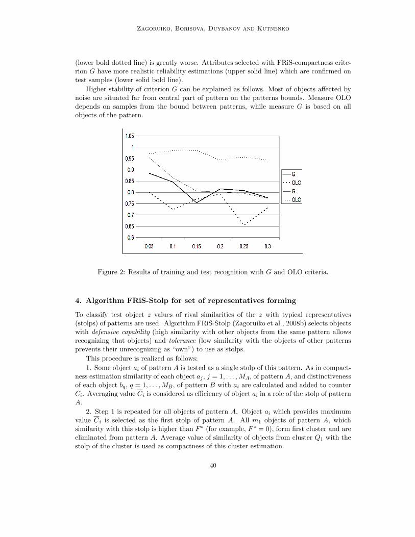
Zagoruiko, Borisova, Duybanov and Kutnenko
(lower bold dotted line) is greatly worse. Attributes selected with FRiS-compactness crite-rion G have more realistic reliability estimations (upper solid line) which are confirmed ontest samples (lower solid bold line).
Higher stability of criterion G can be explained as follows. Most of objects affected bynoise are situated far from central part of pattern on the patterns bounds. Measure OLOdepends on samples from the bound between patterns, while measure G is based on allobjects of the pattern.
Figure 2: Results of training and test recognition with G and OLO criteria.
4. Algorithm FRiS-Stolp for set of representatives forming
To classify test object z values of rival similarities of the z with typical representatives(stolps) of patterns are used. Algorithm FRiS-Stolp (Zagoruiko et al., 2008b) selects objectswith defensive capability (high similarity with other objects from the same pattern allowsrecognizing that objects) and tolerance (low similarity with the objects of other patternsprevents their unrecognizing as “own”) to use as stolps.
This procedure is realized as follows:
1. Some object ai of pattern A is tested as a single stolp of this pattern. As in compact-ness estimation similarity of each object aj , j = 1, . . . , MA, of pattern A, and distinctivenessof each object bq, q = 1, . . . , MB, of pattern B with ai are calculated and added to counterCi. Averaging value Ci is considered as efficiency of object ai in a role of the stolp of patternA.
2. Step 1 is repeated for all objects of pattern A. Object ai which provides maximumvalue Ci is selected as the first stolp of pattern A. All m1 objects of pattern A, whichsimilarity with this stolp is higher than F ∗ (for example, F ∗ = 0), form first cluster and areeliminated from pattern A. Average value of similarity of objects from cluster Q1 with thestolp of the cluster is used as compactness of this cluster estimation.
40
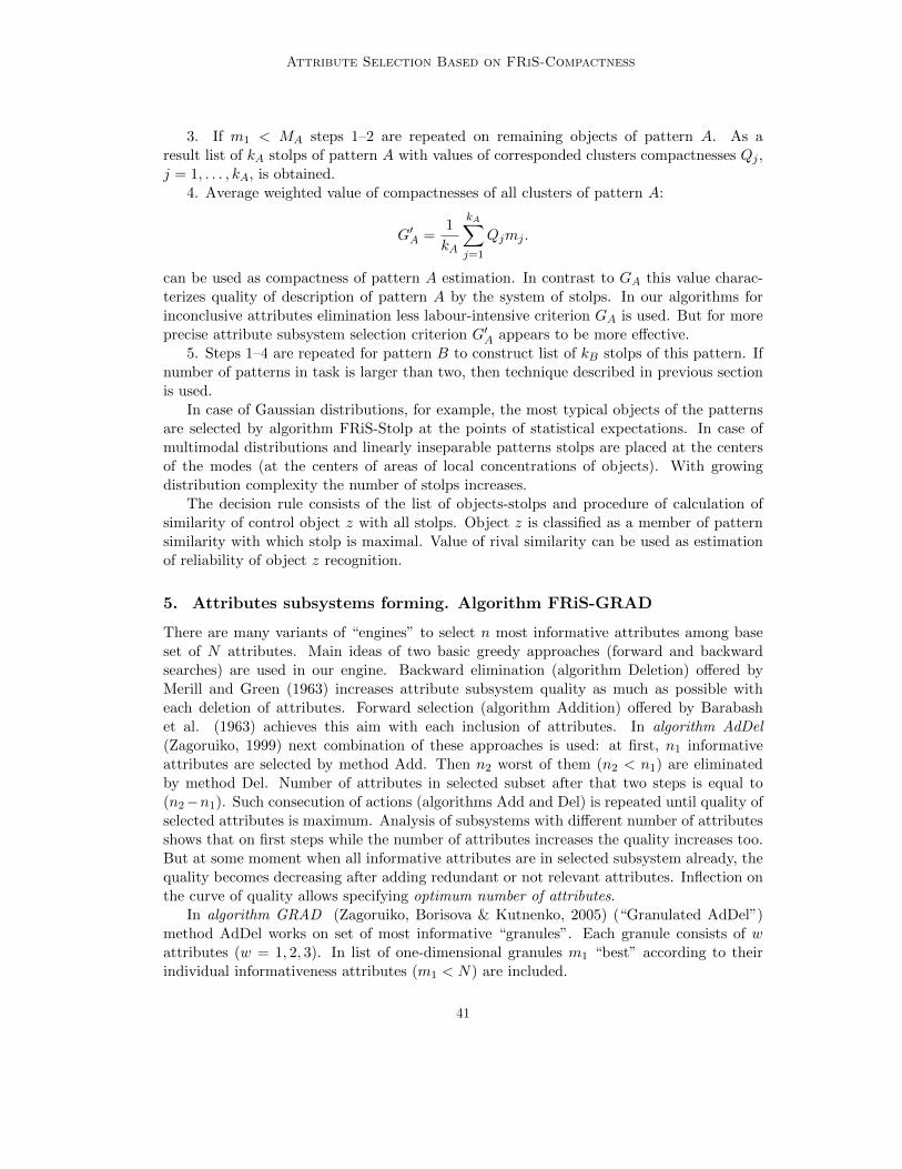
Attribute Selection Based on FRiS-Compactness
3. If m1 < MA steps 1–2 are repeated on remaining objects of pattern A. As aresult list of kA stolps of pattern A with values of corresponded clusters compactnesses Qj ,j = 1, . . . , kA, is obtained.
4. Average weighted value of compactnesses of all clusters of pattern A:
G′A =
1
kA
kA∑
j=1
Qjmj .
can be used as compactness of pattern A estimation. In contrast to GA this value charac-terizes quality of description of pattern A by the system of stolps. In our algorithms forinconclusive attributes elimination less labour-intensive criterion GA is used. But for moreprecise attribute subsystem selection criterion G′
A appears to be more effective.5. Steps 1–4 are repeated for pattern B to construct list of kB stolps of this pattern. If
number of patterns in task is larger than two, then technique described in previous sectionis used.
In case of Gaussian distributions, for example, the most typical objects of the patternsare selected by algorithm FRiS-Stolp at the points of statistical expectations. In case ofmultimodal distributions and linearly inseparable patterns stolps are placed at the centersof the modes (at the centers of areas of local concentrations of objects). With growingdistribution complexity the number of stolps increases.
The decision rule consists of the list of objects-stolps and procedure of calculation ofsimilarity of control object z with all stolps. Object z is classified as a member of patternsimilarity with which stolp is maximal. Value of rival similarity can be used as estimationof reliability of object z recognition.
5. Attributes subsystems forming. Algorithm FRiS-GRAD
There are many variants of “engines” to select n most informative attributes among baseset of N attributes. Main ideas of two basic greedy approaches (forward and backwardsearches) are used in our engine. Backward elimination (algorithm Deletion) offered byMerill and Green (1963) increases attribute subsystem quality as much as possible witheach deletion of attributes. Forward selection (algorithm Addition) offered by Barabashet al. (1963) achieves this aim with each inclusion of attributes. In algorithm AdDel(Zagoruiko, 1999) next combination of these approaches is used: at first, n1 informativeattributes are selected by method Add. Then n2 worst of them (n2 < n1) are eliminatedby method Del. Number of attributes in selected subset after that two steps is equal to(n2 −n1). Such consecution of actions (algorithms Add and Del) is repeated until quality ofselected attributes is maximum. Analysis of subsystems with different number of attributesshows that on first steps while the number of attributes increases the quality increases too.But at some moment when all informative attributes are in selected subsystem already, thequality becomes decreasing after adding redundant or not relevant attributes. Inflection onthe curve of quality allows specifying optimum number of attributes.
In algorithm GRAD (Zagoruiko, Borisova & Kutnenko, 2005) (“Granulated AdDel”)method AdDel works on set of most informative “granules”. Each granule consists of wattributes (w = 1, 2, 3). In list of one-dimensional granules m1 “best” according to theirindividual informativeness attributes (m1 < N) are included.
41

Zagoruiko, Borisova, Duybanov and Kutnenko
Exhaustive search among all possible pairs and triplets of m1 attributes is used form2 two-dimensional and m3 three-dimensional granules forming. Among them m mostinformative granules are selected and used as an input of algorithm AdDel. Comparingeffectiveness of algorithms AdDel and GRAD on different tasks showed, that algorithmGRAD was much better than algorithm AdDel.
To find the best subsystem of attributes and effective decision rule algorithm FRiS-GRAD (Zagoruiko et al., 2008b) uses procedure of directed search, offered in algorithmGRAD. On each step some variant of attribute subsystem is formed and then algorithmFRIS-Stolp is started to construct set of stolps and to calculate FRiS-quality G′ of thesubsystem. If t-dimension subsystem of attributes has been selected and q next stepsof algorithm GRAD working quality of decision was decreasing then this subsystem isconsidered as most informative and set of stolps in this subspace determines the rule toclassify new objects.
6. Recognition of two types of leukemia with algorithm FRiS-GRAD
Efficiency of offered algorithm was demonstrated on task for medical diagnosis (two typesof leukemia recognition). This task was interesting for us because results of its solving bydifferent researchers were published and we could compare effectiveness of our algorithmwith competitors. In the work (Guyon et al., 2002) the best in the world at the moment ofthe publication results obtained by Support Vector Machines (SVM) were presented.
In this task analyzed data set consists of a matrix of gene expression vectors obtainedfrom DNA micro-arrays for a number of patients with two different types of leukemia (ALLand AML) (Golub et al., 1999). Training set consists of 38 samples (27 ALL and 11AML) from bone marrow specimens. The test set has 34 samples (20 ALL and 14 AML).It prepared under different experimental conditions and including 24 bone marrow and 10blood sample specimens. Number of features in the task is 7129. Each attribute correspondsto some normalized gene expression extracted from the micro-array pattern.
The informative subset of attributes in (Guyon et al., 2002) got out by method RFE (aversion of algorithm Deletion). In selected subspace of two best attributes 30 test objectswere correctly recognized, in subspace of 4 attributes number of correctly recognized objectswas 31, in subspace of 128 attributes it was 33. Our results for this task were the following(Zagoruiko et al., 2008b). From 7129 initial attributes algorithm FRiS-GRAD selected 39most informative attributes and constructed 30 decision rules: 27 of them recognized all 34test samples correctly. Ten most informative according their FRiS-compactness G′ attributesubsystems are presented in Table 1. Indexes attached to attribute numbers show weightsof these attributes in decision rules.
These weights are defined by algorithm GRAD. At calculation of distances betweenobjects the values of the attribute with weight v, are multiplied by v.
Offered algorithm is linear. Its laboriousness has the order of complexityO[(N + m3
1/6)M3]. There M is number of objects in the mixed dataset, N is dimensionof features space, m1 — number of attributes used for forming two- and three- dimensiongranules. Here we used m1 = m2 = m3 = 100.
Difference in presented results and results of SVM can be explained by peculiaritiesof as attributes selection method, as algorithm of decision rule construction. To compare
42
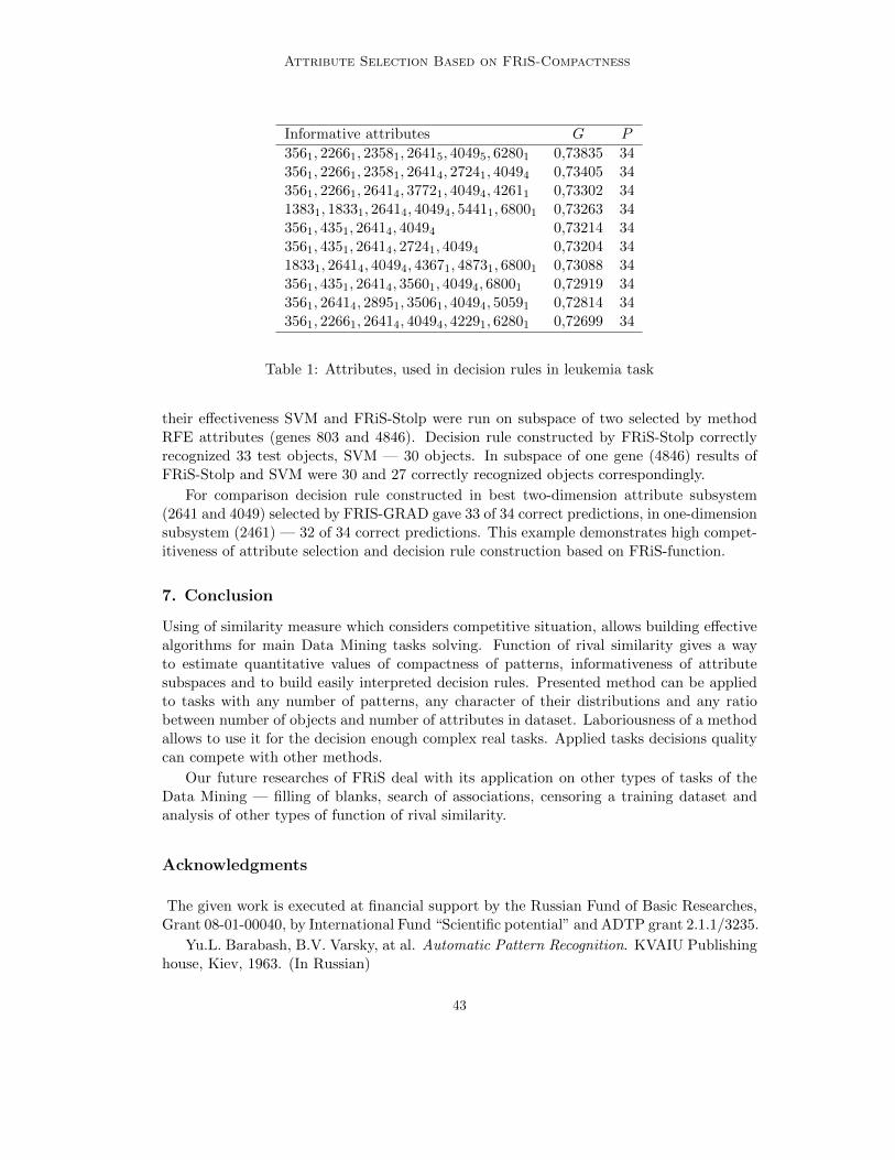
Attribute Selection Based on FRiS-Compactness
Informative attributes G P
3561, 22661, 23581, 26415, 40495, 62801 0,73835 343561, 22661, 23581, 26414, 27241, 40494 0,73405 343561, 22661, 26414, 37721, 40494, 42611 0,73302 3413831, 18331, 26414, 40494, 54411, 68001 0,73263 343561, 4351, 26414, 40494 0,73214 343561, 4351, 26414, 27241, 40494 0,73204 3418331, 26414, 40494, 43671, 48731, 68001 0,73088 343561, 4351, 26414, 35601, 40494, 68001 0,72919 343561, 26414, 28951, 35061, 40494, 50591 0,72814 343561, 22661, 26414, 40494, 42291, 62801 0,72699 34
Table 1: Attributes, used in decision rules in leukemia task
their effectiveness SVM and FRiS-Stolp were run on subspace of two selected by methodRFE attributes (genes 803 and 4846). Decision rule constructed by FRiS-Stolp correctlyrecognized 33 test objects, SVM — 30 objects. In subspace of one gene (4846) results ofFRiS-Stolp and SVM were 30 and 27 correctly recognized objects correspondingly.
For comparison decision rule constructed in best two-dimension attribute subsystem(2641 and 4049) selected by FRIS-GRAD gave 33 of 34 correct predictions, in one-dimensionsubsystem (2461) — 32 of 34 correct predictions. This example demonstrates high compet-itiveness of attribute selection and decision rule construction based on FRiS-function.
7. Conclusion
Using of similarity measure which considers competitive situation, allows building effectivealgorithms for main Data Mining tasks solving. Function of rival similarity gives a wayto estimate quantitative values of compactness of patterns, informativeness of attributesubspaces and to build easily interpreted decision rules. Presented method can be appliedto tasks with any number of patterns, any character of their distributions and any ratiobetween number of objects and number of attributes in dataset. Laboriousness of a methodallows to use it for the decision enough complex real tasks. Applied tasks decisions qualitycan compete with other methods.
Our future researches of FRiS deal with its application on other types of tasks of theData Mining — filling of blanks, search of associations, censoring a training dataset andanalysis of other types of function of rival similarity.
Acknowledgments
The given work is executed at financial support by the Russian Fund of Basic Researches,Grant 08-01-00040, by International Fund “Scientific potential” and ADTP grant 2.1.1/3235.
Yu.L. Barabash, B.V. Varsky, at al. Automatic Pattern Recognition. KVAIU Publishinghouse, Kiev, 1963. (In Russian)
43
Zagoruiko, Borisova, Duybanov and Kutnenko
E.M. Braverman. Experiences on training the machine to recognition of visual patterns.Automatics and Telemechanics, 23(3):349–365, 1962. (In Russian)
E. Fix, J. Hodges. Discriminatory Analysis: Nonparametric Discrimination: Consis-tency Properties. Technical report, USAF School of Aviation Med., Randolph Field, TX,Rep. 21–49–004, 1951.
T.R. Golub, D.K. Slonim, P. Tamayo, C. Huard, M. Gaasenbeek, J.P. Mesirov, H. Coller,M.L. Loh, J.R. Downing, M.A. Caligiuri, C.D. Bloomfield , E.S. Lander. Molecular Classi-fication of Cancer: Class Discovery and Class Prediction by Gene Expression Monitoring.Science, V. 286, 1999.URL: http://www.genome.wi.mit.edu/MPR/data set ALL AML.html.
I. Guyon, J. Weston, S. Barnhill, V. Vapnik. Gene Selection for Cancer Classificationusing Support Vector Machines. Machine Learning, 46(1–3):389–422, 2002.
K. Kira, L. Rendell. The Feature Selection Problem: Traditional Methods and a NewAlgorithm. In Proc. 10 Natl Conf. Artificial Intelligence (AAAI-92), pages 129–134, MenloPark: AAAI Press, 1992.
T. Merill, O.M. Green. On the effectiveness of receptions in recognition systems. IEEETrans. Inform. Theory. IT-9:11–17, 1963.
K.V. Vorontsov, A.O. Koloskov. Support Vectors Selection for Nearest Neighbor Clas-sifier based on Compactness Profile. Artificial Intelligence 2:30–33, 2006. (In Russian)
N.G. Zagoruiko. Applied Methods of Data and Knowledge Analysis. Publishing houseof Institute of Mathematics SD RAS, Novosibirsk, 1999. (In Russian)
N.G. Zagoruiko. Measure of Similarity and Compactness in Competitive Space. InProc. of 8 International Symposium on In Intelligent Data Analysis (IDA-09), pages 369–380, Lion, France, 2009.
N.G. Zagoruiko, I.A. Borisova, O.A. Kutnenko. Informative attribute subspace selection(algorithm GRAD) In Proc. of 12 All-Russian Conf. Mathematical Methods of PatternRecognition (MMRO-12), pages 106–109, Moskow, 2005.
N.G. Zagoruiko, I.A. Borisova, V.V. Dyubanov, O.A. Kutnenko. Methods of RecognitionBased on the Function of Rival Similarity. Pattern Recognition and Image Analysis, 18:1–6,2008. Yu.L.
N.G. Zagoruiko, I.A. Borisova, V.V. Dyubanov, O.A. Kutnenko. Attribute selectionthrough decision rules construction (algorithm FRiS-GRAD). In Proc. of 9 Intern Conf.Pattern Recognition and Image Analysis, V. 2, pages 335–338, Nizhni Novgorod, 2008.
44

JMLR: Workshop and Conference Proceedings 10: 45-54 The Fourth Workshop on Feature Selection in Data Mining
Effective Wrapper-Filter hybridizationthrough GRASP Schemata
M.A. Esseghir [email protected]
Artois University, Faculty of Applied Sciences of Bethune,
TechnoPark Futura, 62400, France.
Editor: Huan Liu, Hiroshi Motoda, Rudy Setiono, and Zheng Zhao
Abstract
Of all of the challenges which face the selection of relevant features for predictive datamining or pattern recognition modeling, the adaptation of computational intelligence tech-niques to feature selection problem requirements is one of the primary impediments. A newimproved metaheuristic based on Greedy Randomized Adaptive Search Procedure (GRASP)is proposed for the problem of Feature Selection. Our devised optimization approach pro-vides an effective scheme for wrapper-filter hybridization through the adaptation of GRASPcomponents. The paper investigates, the GRASP component design as well as its adapta-tion to the feature selection problem. Carried out experiments showed Empirical effective-ness of the devised approach.
Keywords: Feature selection, Combinatorial optimization, Hybrid modeling, GRASP,Local Search.
1. Introduction
Researchers in machine learning, data mining, pattern recognition and statistics have devel-oped a number of methods for dimensionality reduction based on usefulness and classifica-tion accuracy estimates of both individual features and subsets. In fact, Feature Selection(FS) tries to select the most relevant attributes from raw data, and hence guide the con-struction of the final classification model or decision support system. From one hand, themajority, of learning scheme, are being relying on feature selection either as independentpre-processing technique or as an embedded stage within the leaning process (Guyon andElisseff, 2003). On the other hand, both feature selection and data mining techniques strug-gle to gain the attended reliability, especially, when they face high dimensional data (Liuand Motoda, 2008).
In this paper, we propose, a new hybrid search technique through the adaptation ofthe GRASP heuristic to the FS problem. The devised approach investigates the effectivewrapper-filter combination by exploiting the intrinsic properties of the GRASP heuristic.The main motivations for this proposal are three folds: (i) filter-wrapper collaborationmight enhance the relevance of the selected feature subsets (ii) local search approaches haveshown their effectiveness in FS with both sequential deterministic procedures (i.e. SFFS(Somol et al., 1999), IFFS (Nakariyakul and Casasent, 2009), etc) and stochastic approaches(i.e. Hill Climbing (Kohavi and John, 1997), Simulated Annealing (Guyon et al., 2006) andTabu search (Yus, 2009)). The GRASP is a multi-start heuristic based on local search (iii)
c©2010 Esseghir.
Esseghir
endowing basic sequential search procedures with both filter guidance and the stochasticability to alleviate FS challenging problems like local minimas and nesting effect (Guyonet al., 2006; Liu and Motoda, 2008).
The remainder of this paper is organized in five sections. Section 2 formalizes thefeature selection problem and gives an overview of representative approaches. Section 3briefly introduces the GRASP heuristic as well as its recent application to feature selection.Section 4 details the devised GRASP for FS. Section 5 compares and assesses GRASPalternatives behaviors empirically. Finally, Section 6 concludes the paper and provide somedirections of future research.
2. Feature selection: basics and background
Let D be a data set with F as a set of features such that |F | = n, and let X (X ⊆ F ) bea subset of F . Let J(X) the function that assesses the relevance of the features subset X.The problem of feature selection states the selection of a subset Z such that:
J(Z) = maxX⊆FJ(X) (1)
In other words, the retained feature subset should be compact and representative of thedataset objects or the underlying context. This might be done by both removing redundantnoisy or/and irrelevant attributes by keeping the minimal information loss.
For a given dataset of n features, the exploration would require the examination of2n possible subsets. Consequently, the search through the feasible solutions search spaceis a np-hard combinatorial problem (Liu and Motoda, 2008). An exhaustive explorationof the feature space seems to be impractical, especially, when n became large or evenmoderate. Numerous reference approaches have been proposed for the identification ofsalient features with the highest predictive power (Guyon et al., 2006; Liu and Motoda,2008). The representative approaches could be, broadly, categorized into two classes: filtersand wrappers (Guyon and Elisseff, 2003; Guyon et al., 2006).
Filters
Considered as the earliest approaches to feature selection, filter methods discard irrele-vant features, without any reference to a data mining technique, by applying independentsearch which is mainly based on the assessment of intrinsic attribute properties and theirrelationship with the data set class (i.e. Relief, Symmetrical uncertainty, Pearson corre-lation, etc) (Liu and Motoda, 2008). The main advantage of the filter methods is theirreduced computational complexity which is due to the simple independent criterion used forfeature evaluation. In most of the cases, filters provide a ranking based on scores reflectingattribute usefulness to the class.
Wrappers
When feature selection is based on a wrapper, attributes are simultaneously evaluatedusing a classification algorithm. The subset exploration requires a heuristic search strat-egy. Kohavi et al. (Kohavi and John, 1997) were the first to advocate the wrapper as ageneral framework for feature selection in machine learning. Numerous studies have usedthe above framework with different combinations of the evaluation and search components.Featured search technique are ranging from greedy sequential attribute selection methods
46

Adaptive Feature Selection
(i.e. SFS, SBE, Floating search (Somol et al., 1999)) to randomized and stochastic meth-ods (i.e. GRASP (Yus, 2009), TABU, BEAM, Genetic Algorithm (Guyon et al., 2006)) .The wrapper methods often provide better results than filter ones because they considera classifier within the evaluation process. We should note that feature selection methodsbased on wrappers are computationally expensive compared to filters, due to the cost ofiterative running of the classification algorithm (Guyon and Elisseff, 2003).
The motivation to hybrid approaches design is the exhibited multidisciplinary problemnature and the need to overcome the pitfalls of one approach by the advantage of the otherone. The simplest form of recombination is to use both filters and wrappers. The commonscheme of combination entails a couple of steps. The first one applies filter to reduce thesearch space, while the second step explores with a wrapper the subsets built from theyielded features returned by the first step (Liu and Motoda, 2008).
3. GRASP
This section covers paper materials by introducing GRASP heuristic principle, componentsand its recent application to feature selection modeling. The Greedy Randomized searchprocedure (GRASP) is meta-heuristic for combinatorial optimization problems (Resende,1999; Resende et al., 2002). Usually known as multi-start procedure, GRASP is based onan iterative process which constructs a solution then fine tune it, through a local search.The multi-start property enlarges the search coverage by exploring different regions of thesearch space without being influenced by the previous solutions found.
GRASP heuristic was successfully applied to numerous combinatorial problem rangingfrom scheduling (Aiex et al., 2003) and quadratic assignment (Ahuja et al., 2000) to datamining (Ahmadi and Osman, 2005).
3.1 GRASP Components
The recent optimization scheme proposed by GRASP (Resende, 1999) applyies an iterativelocal search scheme based on incremental solution construction and neighborhood explo-ration. The iterative process consists of two stages: the construction of a feasible solutionand local search.
The construction stage builds a solution, incrementally, using a Restricted List of Can-didates RCL The RCL is, generally, formed by the best solution elements (i.e. elementswhich can improve the current solution). Solutions are built using a random selection fromthe RCL.
Once the solution is generated, it passes through the second stage. Within the secondstage the solution is iteratively, refined by local search until it reaches a local optima. Thisprocedure is mainly based on neighborhood generation and the exchange of the currentsolution by the best solution among neighbors. The procedure restarts until no improvementcould be gained. The pseudo-codes of both GRASP local search (LS) procedures adaptedto the problem of FS will be detailed, below, by Algorithm 1 and 2 in the following section.
The multi-start property of GRASP allows the search process to be not trapped in localminima and to explore different regions of the search space, without being constrained orinfluenced by the best solution found.
47

Esseghir
Algorithm 1: G.R.A.S.P.
Input:F : Initial Feature setC: Target class Attributeβ: Thresholdd: number of attributes to selectnmax: attempts numberOutput:Sbest : Selected FeaturesBegin1
S ← ∅2
Sbest ← S3
While Stop Criterion not4
Satisfied do//Construction stage5
Foreach fi ∈ F do6
gi ← IGV (fi, C)7
Sollist ← ∅8
repeat9
S ← ∅10
repeat11
min← argmini(gi),12
max← argmaxi(gi)RCLlist = vj , gj ≤13
α.gmax + (1− α)gminRandomly select vj ∈14
vj ∈ RCLlist, vj /∈ SS ← S ∪ vj15
RCL← RCL \ vj16
until |S| == d;17
S.fitness=Evaluate(S,Cla)18
Sollist ← S ∪ Sollist19
until |Sollist| = nmax;20
S ← getBest(Sollist);21
// iterative local search22
S ← LocalSearch(S)23
If S.fitness > Sbest.fitness24
thenSbest ← S25
Return (Sbest)26
End27
Algorithm 2: Iterative Local Searchprocedure
Input:F : Initial Feature setC: Target class AttributeCla: a classifier for solution evaluationS: input SolutionOutput:S’ : result of local searchBegin1
S1← S , Sbest ← S12
Stop ← false3
repeat4
Sollist ← NH(S1, F )5
∀X ∈ Sollist, Evaluate(X,Cla)6
S1← getBest(Sollist)7
If S1.fitness > Sbest.fitness8
thenSbest ← S19
Else10
Stop ← true11
until (Stop = true);12
S’← Sbest13
Return (S’ )14
End15
48

Adaptive Feature Selection
3.2 GRASP for Feature Selection
The application of GRASP to the FS problem was, recently provided by Yusta in (Yus,2009). The proposed GRASP was compared to effective FS search techniques like to geneticalgorithms, tabu search and SFFS.
The GRASP proposed in (Yus, 2009), is illustrated by Algorithm 1. The algorithmis based on two main stages, namely solution construction (Lines 6-21) and local searchprocedure (see Algorithm 2). The first stage constructs a fixed number of solutions (nmax),and the best one will be selected as a candidate for the second stage.Solution are constructedaccording to the attributes retained by the RCL list. The RCL is based on the In-GroupVariability (IGV function) criterion (see eq. 2).
IGV (fj , C) =∑
i
(f ij − µC(i))2 (2)
Where f ji and µC(i) denote respectively the i-th value of the attribute fj and the meanµC(i) of fj values for the instances belonging to the same class as the instance i. Besidesthe attribute selection, is controlled by the parameter α (Lines 11-17). In fact, it controlsthe degree of randomness of the procedure.
The second stage applies a hill climbing procedure to the solution provided by the firststage. The pseudo-code of the iterative LS is illustrated by algorithm 2. Each iterationgenerates neighborhood solutions and exchange current solution with best neighbors if itcan improve classification accuracy. The neighborhood structure proposed, by Yusta in(Yus, 2009), is based on attribute replacement and is given by the equation 3:
NH(S) = X,X = S ∪ fi \ fj,∀fi ∈ F \ S, ∀fj ∈ S (3)
Such a neighborhood structure NH(S) consider all combinations of attribute exchange.Consequently, LS is sensitive to the number of selected features. The neighborhood explo-ration becomes prohibitive even for moderate value of n. The computational complexity isin the order of O(p ∗m). 1
4. Proposed GRASP-FS
In this section, we investigate, the proposed a new GRASP schemata for FS. We focus ona set commonly used local search procedures and filters. Next, we try to adapt and deploythem as GRASP components.
Since the GRASP scheme is based on a restricted list of candidates, this list could berepresented by features that seems to be relevant or those that might provide incrementalusefulness to the selected feature subset. For the GRASP construction stage we opt forselection scheme capable of generating attribute ranking. Hence, the score associated tofeatures will serve as selection criterion for the RCL generation. The second stage of GRASPtries to enhance solutions by an iterative neighborhood exploration. The subsets are assessedaccording to a classification criterion (i.e. generalization error rate). The quality of solutionfine-tuning, mainly, depends on the nature of the involved neighborhood structure of LS.
1. p and m respectively denote the number of selected and non-selected features (p + m = n).
49
Esseghir
We devise a number of LS procedures based on different neighborhood structures in-spired from well known sequential search procedures. The following two sections, detaildifferent design alternatives for both RCL and local search GRASP component.
4.1 RCL generation
Comparatively to the GRASP scheme proposed by Yusta in (Yus, 2009), the same con-struction phase steps (see Algo. 1 Lines 6-21) are adopted, except the procedure whichgenerates the RCL the (see Algo. 1 Line 6-7).
Any filter criterion could be, instead, used to build RCL. In this paper, we opt for threewell known and different selection schema: ReliefF (Robnik-Sikonja and Kononenko, 1997),Symmetrical Uncertainty (SU) (Guyon et al., 2006), and FCBF (Yu and Liu, 2003).
Typically, filters return solutions based on the selection of features with the highestscores. Once the initial RCL is generated2 , the variables are randomly selected to buildGRASP first stage solutions. Such a selection schema have, at least, tow benefits: (i)reducing the risk of selection of, only, highly correlated relevant features (ii) the combinationof features with moderate usefulness, which are not highly relevant to the target, mightpromote interaction among selected attributes.
4.2 Local Search Procedures
The local search (LS) is applied at the second stage of the GRASP. It aims at the improve-ment of the solution provided by the GRASP first stage process. An interesting aspectthat could motivate the wrapper choice as component of the GRASP second stage, is thesuccessful application of local search methods in FS modeling (i.e. Tabu search, Simulatedannealing, Hill climbing) (Guyon et al., 2006).
In this paper, we devise effective LS procedures inspired from successfully search tech-niques adapted to the FS. The following paragraphs detail the neighborhood structures thatwill be deployed within the local search procedures. They will be, also, discussed in thecontext of FS search space exploration.
Bit-Flip Local search (BF) explores neighboring solutions by adding or removing onefeature at a time. For solutions encoded with binary strings this operator inverts one bitvalue for each neighbor. In comparison to the sequential search procedures, the generatedneighborhood covers both solutions explored in SFS (see eq. 5) and SBE (see eq. 6) Thebit-Flip operator (BF) neighborhood is illustrated by the equation 4.
NHBF (S) = X|X = NH+(S) ∪NH−(S) (4)
NH+(S) = X|X = S ∪ fi,∀fi ∈ F, fi /∈ S (5)
NH−(S) = X|X = S \ fi,∀fi ∈ S (6)
The problem of nesting effect encountered with both sequential forward and backwardprocedures is alleviated by the merge of the neighborhoods explored by both procedures.
2. using filter criterion
50

Adaptive Feature Selection
Attribute-Flip (AF) local search procedure constructs neighborhood using a per-mutation between a selected and a non-selected features (see eq. 3). This neighborhoodstructure was used, by Yusta in (Yus, 2009), as a local search procedure. The two opera-tors explore different region of the current solution neighborhood. There is no overlappingregions (NHBF (S)∩NHAF (S) = ∅) and the second neighborhood structure is much largerthan the first which would require more computational time.
Local search based floating search (SFFS1). Since, SFS and SBE approachescould be seen as local search procedures, floating searches (SFFS and SFBS) could be alsoconsidered as an improved version of both sequential procedures and their associated localsearch. In fact, solutions explored by an iteration of SFFS are those generated by theunion of NH1 = NH+(S) and the conditional application of the backward search to thebest improvement provided by NH1. Note that the LS based on SFFS1 neighborhood isnot comparable to that using AF local search. AF applies NH+(.) and NH−(.) to thesame initial solution while, with SFF1, NH−(.) is applied to the improved solution afterthe application of NH+(.). Besides, there is no risk of cycling, because the Neighborhoodprocedures are only applied to improved solutions.
Local search based floating search 2 (SFF2) In the case of SFF2, the same floatingsearch scheme as in SFF1 is adopted, however the backward procedure NH−(.) is notapplied once but the backtrack is applied iteratively repeated until no improvement can bereached. Comparatively to SFF1, SFF2 requires more computational time than the firstfloating alternative but might lead to more compact subset size.
5. Empirical study
In this section, we empirically assess the behavior of proposed GRASP schema as wellas a selection of the devised components. They will be, also, compared to the baselineGRASP 〈IGV,AF 〉 proposed by Yusta in (Yus, 2009), where reported results have confirmedthe superiority of GRASP over Tabu search, Genetic and Memetic algorithms, and SFFSapproach.
Five benchmark datasets were used to validate GRASP components: Sonar, Ionosphere,SpamBase, Audiology and Arrhythmia with respectively 60, 34, 57, 69 and 279 attributes.These datasets are provided by the UCI repository (Blake and Merz, 1998). Reportedresults, correspond to the average values of at least 50 trial runs. Means, Standard deviationand statistical test validation (t-Test with confidence level of 97.5%) are also provided.
Two types of results are proposed: (i) those corresponding to the best solution fitness(generalization error rate) yielded from the GRASP search. K-Nearest Neighbors (KNN) isused as wrapper classifier (K = 3) (ii) the validation on independent data set instances ofthe resulting features subsets using Artificial neural network (ANN) and Naive Bayes(Guyonet al., 2006). The selection of different classification paradigms for both search and vali-dation make the validation less biased and independent of wrapper classifier. Besides, thevalidation stage is based on 10-folds cross-validation technique.
51
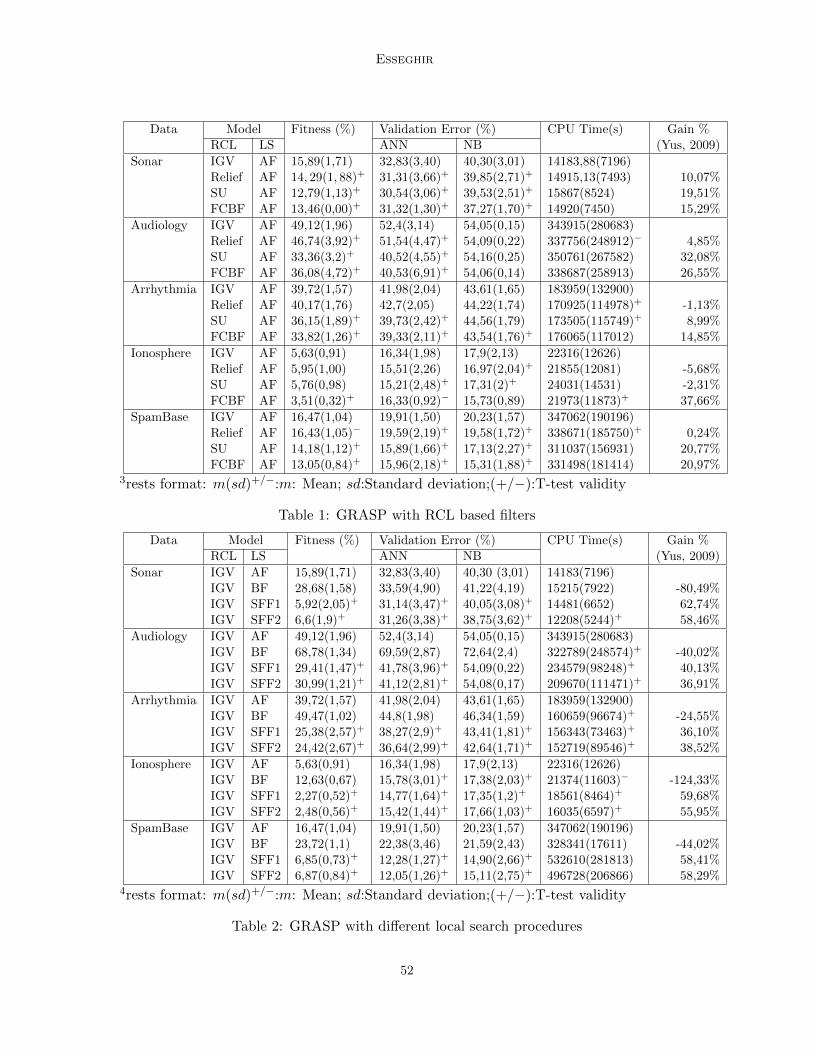
Esseghir
Data Model Fitness (%) Validation Error (%) CPU Time(s) Gain %RCL LS ANN NB (Yus, 2009)
Sonar IGV AF 15,89(1,71) 32,83(3,40) 40,30(3,01) 14183,88(7196)Relief AF 14, 29(1, 88)+ 31,31(3,66)+ 39,85(2,71)+ 14915,13(7493) 10,07%SU AF 12,79(1,13)+ 30,54(3,06)+ 39,53(2,51)+ 15867(8524) 19,51%FCBF AF 13,46(0,00)+ 31,32(1,30)+ 37,27(1,70)+ 14920(7450) 15,29%
Audiology IGV AF 49,12(1,96) 52,4(3,14) 54,05(0,15) 343915(280683)Relief AF 46,74(3,92)+ 51,54(4,47)+ 54,09(0,22) 337756(248912)− 4,85%SU AF 33,36(3,2)+ 40,52(4,55)+ 54,16(0,25) 350761(267582) 32,08%FCBF AF 36,08(4,72)+ 40,53(6,91)+ 54,06(0,14) 338687(258913) 26,55%
Arrhythmia IGV AF 39,72(1,57) 41,98(2,04) 43,61(1,65) 183959(132900)Relief AF 40,17(1,76) 42,7(2,05) 44,22(1,74) 170925(114978)+ -1,13%SU AF 36,15(1,89)+ 39,73(2,42)+ 44,56(1,79) 173505(115749)+ 8,99%FCBF AF 33,82(1,26)+ 39,33(2,11)+ 43,54(1,76)+ 176065(117012) 14,85%
Ionosphere IGV AF 5,63(0,91) 16,34(1,98) 17,9(2,13) 22316(12626)Relief AF 5,95(1,00) 15,51(2,26) 16,97(2,04)+ 21855(12081) -5,68%SU AF 5,76(0,98) 15,21(2,48)+ 17,31(2)+ 24031(14531) -2,31%FCBF AF 3,51(0,32)+ 16,33(0,92)− 15,73(0,89) 21973(11873)+ 37,66%
SpamBase IGV AF 16,47(1,04) 19,91(1,50) 20,23(1,57) 347062(190196)Relief AF 16,43(1,05)− 19,59(2,19)+ 19,58(1,72)+ 338671(185750)+ 0,24%SU AF 14,18(1,12)+ 15,89(1,66)+ 17,13(2,27)+ 311037(156931) 20,77%FCBF AF 13,05(0,84)+ 15,96(2,18)+ 15,31(1,88)+ 331498(181414) 20,97%
3rests format: m(sd)+/−:m: Mean; sd:Standard deviation;(+/−):T-test validity
Table 1: GRASP with RCL based filters
Data Model Fitness (%) Validation Error (%) CPU Time(s) Gain %RCL LS ANN NB (Yus, 2009)
Sonar IGV AF 15,89(1,71) 32,83(3,40) 40,30 (3,01) 14183(7196)IGV BF 28,68(1,58) 33,59(4,90) 41,22(4,19) 15215(7922) -80,49%IGV SFF1 5,92(2,05)+ 31,14(3,47)+ 40,05(3,08)+ 14481(6652) 62,74%IGV SFF2 6,6(1,9)+ 31,26(3,38)+ 38,75(3,62)+ 12208(5244)+ 58,46%
Audiology IGV AF 49,12(1,96) 52,4(3,14) 54,05(0,15) 343915(280683)IGV BF 68,78(1,34) 69,59(2,87) 72,64(2,4) 322789(248574)+ -40,02%IGV SFF1 29,41(1,47)+ 41,78(3,96)+ 54,09(0,22) 234579(98248)+ 40,13%IGV SFF2 30,99(1,21)+ 41,12(2,81)+ 54,08(0,17) 209670(111471)+ 36,91%
Arrhythmia IGV AF 39,72(1,57) 41,98(2,04) 43,61(1,65) 183959(132900)IGV BF 49,47(1,02) 44,8(1,98) 46,34(1,59) 160659(96674)+ -24,55%IGV SFF1 25,38(2,57)+ 38,27(2,9)+ 43,41(1,81)+ 156343(73463)+ 36,10%IGV SFF2 24,42(2,67)+ 36,64(2,99)+ 42,64(1,71)+ 152719(89546)+ 38,52%
Ionosphere IGV AF 5,63(0,91) 16,34(1,98) 17,9(2,13) 22316(12626)IGV BF 12,63(0,67) 15,78(3,01)+ 17,38(2,03)+ 21374(11603)− -124,33%IGV SFF1 2,27(0,52)+ 14,77(1,64)+ 17,35(1,2)+ 18561(8464)+ 59,68%IGV SFF2 2,48(0,56)+ 15,42(1,44)+ 17,66(1,03)+ 16035(6597)+ 55,95%
SpamBase IGV AF 16,47(1,04) 19,91(1,50) 20,23(1,57) 347062(190196)IGV BF 23,72(1,1) 22,38(3,46) 21,59(2,43) 328341(17611) -44,02%IGV SFF1 6,85(0,73)+ 12,28(1,27)+ 14,90(2,66)+ 532610(281813) 58,41%IGV SFF2 6,87(0,84)+ 12,05(1,26)+ 15,11(2,75)+ 496728(206866) 58,29%
4rests format: m(sd)+/−:m: Mean; sd:Standard deviation;(+/−):T-test validity
Table 2: GRASP with different local search procedures
52

Adaptive Feature Selection
5.1 Construction Phase
In the first stage of the empirical study, we assess the behaviors of the baseline GRASPwith the devised GRASP scheme which is based on Filters to both built RCL and constructsolutions.
For each experiment we present, for each dataset, on columns, best solution fitness (low-est error rate %), test accuracy on independent dataset, average runtime CPU, cardinalityof best solution (#features) and the gain Toward Baseline GRASP fitness. In Additionto the, average , standard deviation values of the different trials, t-test was used for theassessment of the statistical validity of the obtained results toward the baseline method.Table 1 provides results for each data set. Globally, according to the gain (last column)obtained with a GRASP scheme generating the RCL with filters, the baseline method isoutperformed in most of the cases.
Fortunately, the improvement obtained with fitness values is confirmed with validationstage (independent data, and different classification techniques for validation). In most ofthe cases the mean values and t-tests showed decrease of the generalization errors. Theoverall improvement, points out the reliability of the approach, particularly the filters en-listed in the selection of suitable features. All filters enhance at least once, both fitness andvalidation accuracies. Surprisingly, Relief scores used in the RCL build, seems to be theless relevant filter used in the first stage of GRASP whereas GRASP alternatives based onFCBF confirm a slight superiority over those ones using SU.
5.2 Local search enhancement
The local search of the baseline method uses Attribute Flip neighborhood whereas the pro-posed GRASP uses local search procedures inspired from deterministic sequential searches.
The devised local search procedures are deployed within new GRASP instances usingthe IGV criterion on the First stage. Table 2 compare and evaluate the fours GRASPinstances. Even though, the solutions provided by the first GRASP stage are based onIGV criterion, some of the devised local search procedures have succeed to outperform thebaseline algorithm. Indeed, local search alternatives adopting floating selection, have empir-ically confirmed their superiority over Yusta GRASP. On the other hand, the neighborhoodstructure based on the selection or removal of one attribute (NHBF ), the less effective finetuning scheme.
Besides, the overall improvement of the new devised GRASP local search proceduresare most significant that the improvements afforded by the use of filters. In any case, theadapted new GRASP scheme is based have empirically shown that enhancements could beafforded by filters in first stage as well as wrappers in second stage.
6. Conclusion
We devise a new GRASP approach for feature selection capable of hybridizing filters andwrappers. The effectiveness of the different GRASP components combinations were assessedempirically. Carried out results, confirms the robustness of the hybridization schemata andmotivates us to investigate in depth both algorithmic and behavioral aspects of furthercombinations issues, scalability study, and adaptation to high dimensional problems.
53
Esseghir
References
Different metaheuristic strategies to solve the feature selection problem. Pattern RecognitionLetters, 30(5):525 – 534, 2009. ISSN 0167-8655.
Samad Ahmadi and Ibrahim H. Osman. Greedy random adaptive memory programmingsearch for the capacitated clustering problem. European Journal of Operational Research,162(1):30–44, 2005.
R.K. Ahuja, J.B. Orlin, and A. Tiwari. A greedy genetic algorithm for the quadraticassignment problem. Computers and Operations Research, 27:917–934, 2000.
R.M. Aiex, S. Binato, and M.G.C. Resende. Parallel GRASP with path-relinking for jobshop scheduling. Parallel Computing, 29:393–430, 2003.
C. Blake and C. Merz. UCI repository of machine learning databases, 1998). (http:/www.ics.uci.edu/ mlearn/MLRepository.html.
I. Guyon and A. Elisseff. An introduction to variable and feature selection. Journal ofMachine Learning Research, 3:1157–1182, March 2003.
I. Guyon, S. Gunn, M. Nikravesh, and L. Zadeh. Feature Extraction, Foundations andApplications. Series Studies in Fuzziness and Soft Computing. Springer, 2006.
R. Kohavi and G. H. John. Wrappers for feature subset selection. Artificial Intelligence,97:273–324, 1997.
H. Liu and H. Motoda. Computational methods of feature selection. Chapman andHall/CRC Editions, 2008.
Songyot Nakariyakul and David P. Casasent. An improvement on floating search algorithmsfor feature subset selection. Pattern Recogn., 42(9):1932–1940, 2009. ISSN 0031-3203.
Mauricio G. C. Resende. Greedy randomized adaptive search procedures (grasp). Journalof Global Optimization, 6:109–133, 1999.
Mauricio G. C. Resende, Mauricio G. C, Resende, and Celso C. Ribeiro. Greedy randomizedadaptive search procedures, 2002.
Marko Robnik-Sikonja and Igor Kononenko. An adaptation of relief for attribute estimationin regression. In ICML, pages 296–304, 1997.
P. Somol, P. Pudil, J. Novovicova, and P. Paclık. Adaptive floating search methods infeature selection. Pattern Recogn. Lett., 20(11-13):1157–1163, 1999. ISSN 0167-8655.
L. Yu and H. Liu. Feature selection for high-dimensional data: A fast correlation-basedfilter solution. pages 856–863. Twentieth International Conference on Machine Leaning(ICML), 2003.
54
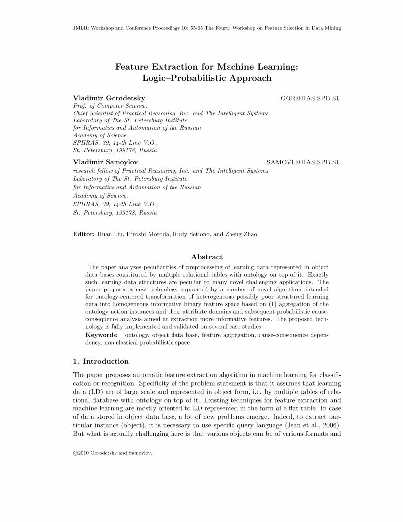
JMLR: Workshop and Conference Proceedings 10: 55-65 The Fourth Workshop on Feature Selection in Data Mining
Feature Extraction for Machine Learning:Logic–Probabilistic Approach
Vladimir Gorodetsky [email protected]. of Computer Science,Chief Scientist of Practical Reasoning, Inc. and The Intelligent SystemsLaboratory of The St. Petersburg Institutefor Informatics and Automation of the RussianAcademy of Science.SPIIRAS, 39, 14-th Line V.O.,St. Petersburg, 199178, Russia
Vladimir Samoylov [email protected]
research fellow of Practical Reasoning, Inc. and The Intelligent Systems
Laboratory of The St. Petersburg Institute
for Informatics and Automation of the Russian
Academy of Science.
SPIIRAS, 39, 14-th Line V.O.,
St. Petersburg, 199178, Russia
Editor: Huan Liu, Hiroshi Motoda, Rudy Setiono, and Zheng Zhao
Abstract
The paper analyzes peculiarities of preprocessing of learning data represented in objectdata bases constituted by multiple relational tables with ontology on top of it. Exactlysuch learning data structures are peculiar to many novel challenging applications. Thepaper proposes a new technology supported by a number of novel algorithms intendedfor ontology-centered transformation of heterogeneous possibly poor structured learningdata into homogeneous informative binary feature space based on (1) aggregation of theontology notion instances and their attribute domains and subsequent probabilistic cause-consequence analysis aimed at extraction more informative features. The proposed tech-nology is fully implemented and validated on several case studies.
Keywords: ontology, object data base, feature aggregation, cause-consequence depen-dency, non-classical probabilistic space
1. Introduction
The paper proposes automatic feature extraction algorithm in machine learning for classifi-cation or recognition. Specificity of the problem statement is that it assumes that learningdata (LD) are of large scale and represented in object form, i.e. by multiple tables of rela-tional database with ontology on top of it. Existing techniques for feature extraction andmachine learning are mostly oriented to LD represented in the form of a flat table. In caseof data stored in object data base, a lot of new problems emerge. Indeed, to extract par-ticular instance (object), it is necessary to use specific query language (Jean et al., 2006).But what is actually challenging here is that various objects can be of various formats and
c⃝2010 Gorodetsky and Samoylov.
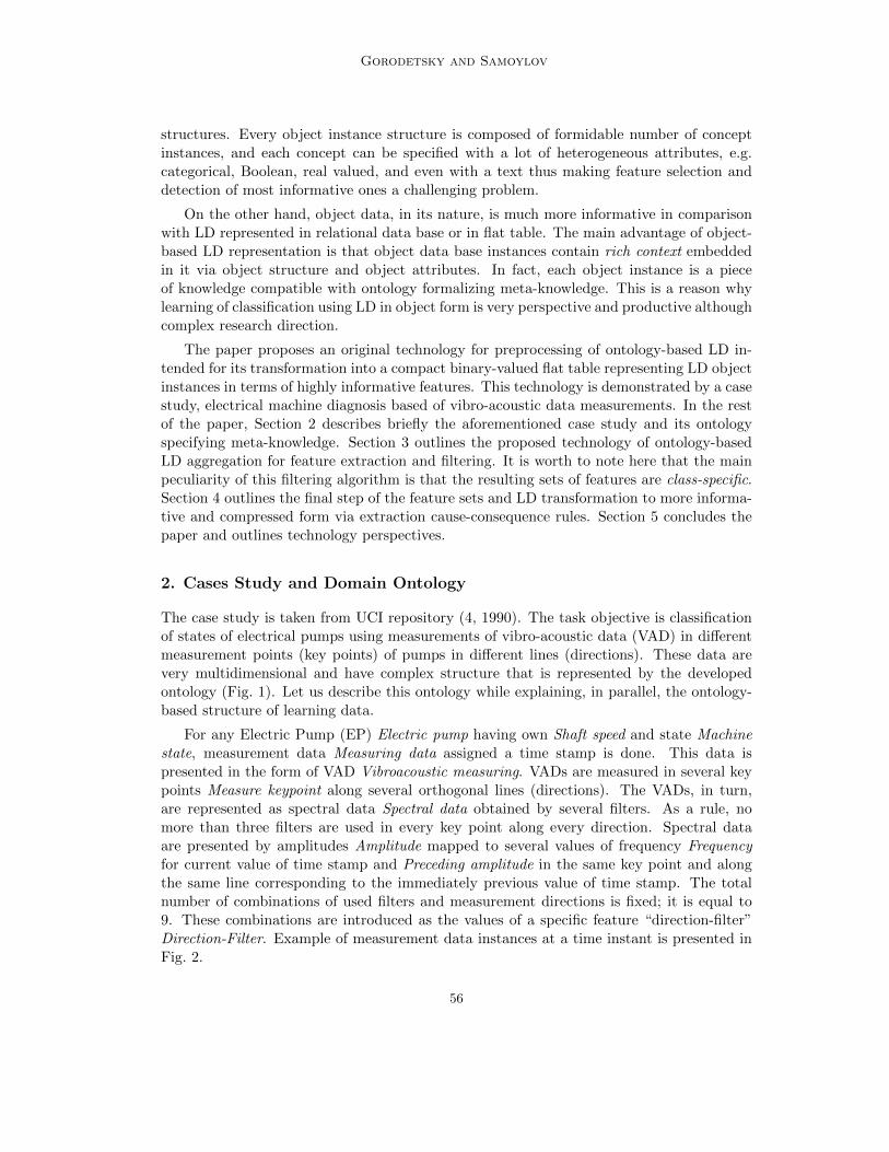
Gorodetsky and Samoylov
structures. Every object instance structure is composed of formidable number of conceptinstances, and each concept can be specified with a lot of heterogeneous attributes, e.g.categorical, Boolean, real valued, and even with a text thus making feature selection anddetection of most informative ones a challenging problem.
On the other hand, object data, in its nature, is much more informative in comparisonwith LD represented in relational data base or in flat table. The main advantage of object-based LD representation is that object data base instances contain rich context embeddedin it via object structure and object attributes. In fact, each object instance is a pieceof knowledge compatible with ontology formalizing meta-knowledge. This is a reason whylearning of classification using LD in object form is very perspective and productive althoughcomplex research direction.
The paper proposes an original technology for preprocessing of ontology-based LD in-tended for its transformation into a compact binary-valued flat table representing LD objectinstances in terms of highly informative features. This technology is demonstrated by a casestudy, electrical machine diagnosis based of vibro-acoustic data measurements. In the restof the paper, Section 2 describes briefly the aforementioned case study and its ontologyspecifying meta-knowledge. Section 3 outlines the proposed technology of ontology-basedLD aggregation for feature extraction and filtering. It is worth to note here that the mainpeculiarity of this filtering algorithm is that the resulting sets of features are class-specific.Section 4 outlines the final step of the feature sets and LD transformation to more informa-tive and compressed form via extraction cause-consequence rules. Section 5 concludes thepaper and outlines technology perspectives.
2. Cases Study and Domain Ontology
The case study is taken from UCI repository (4, 1990). The task objective is classificationof states of electrical pumps using measurements of vibro-acoustic data (VAD) in differentmeasurement points (key points) of pumps in different lines (directions). These data arevery multidimensional and have complex structure that is represented by the developedontology (Fig. 1). Let us describe this ontology while explaining, in parallel, the ontology-based structure of learning data.
For any Electric Pump (EP) Electric pump having own Shaft speed and state Machinestate, measurement data Measuring data assigned a time stamp is done. This data ispresented in the form of VAD Vibroacoustic measuring. VADs are measured in several keypoints Measure keypoint along several orthogonal lines (directions). The VADs, in turn,are represented as spectral data Spectral data obtained by several filters. As a rule, nomore than three filters are used in every key point along every direction. Spectral dataare presented by amplitudes Amplitude mapped to several values of frequency Frequencyfor current value of time stamp and Preceding amplitude in the same key point and alongthe same line corresponding to the immediately previous value of time stamp. The totalnumber of combinations of used filters and measurement directions is fixed; it is equal to9. These combinations are introduced as the values of a specific feature “direction-filter”Direction-Filter. Example of measurement data instances at a time instant is presented inFig. 2.
56
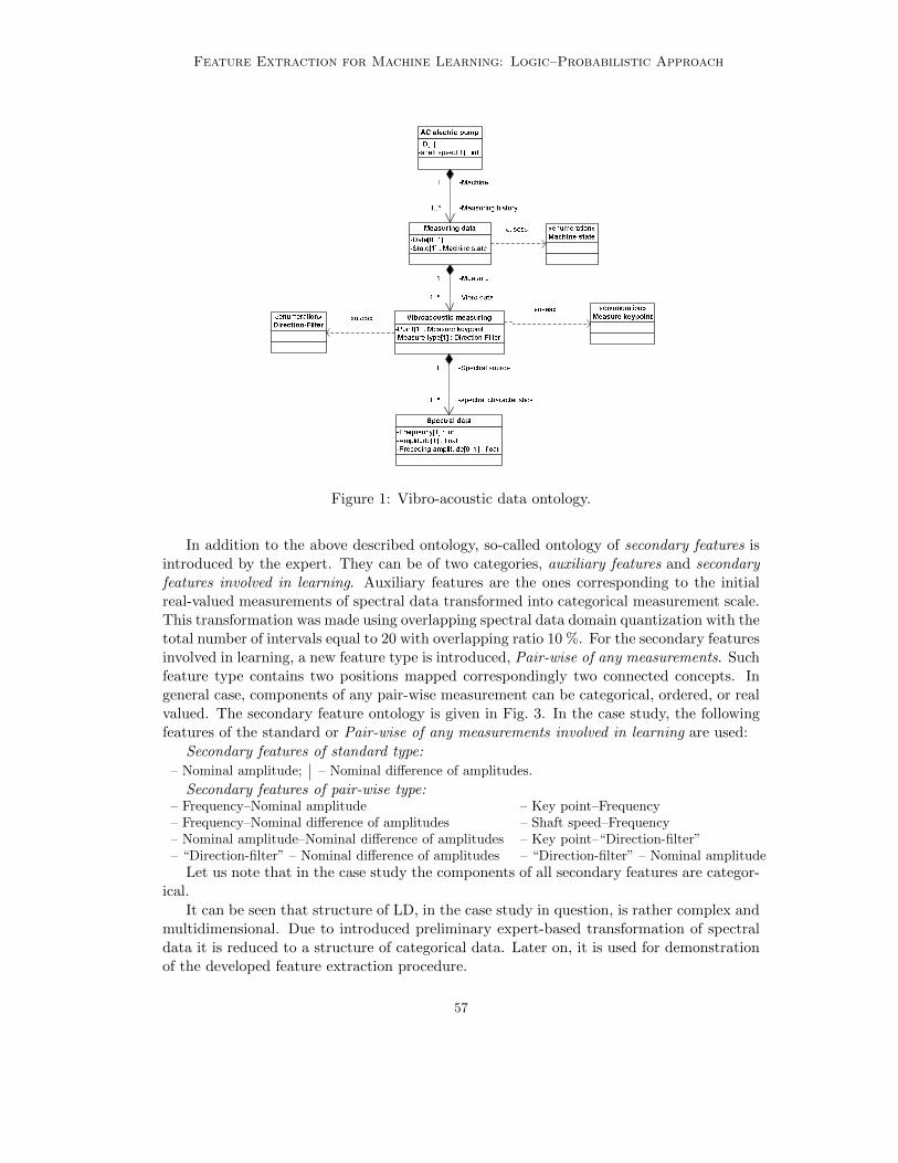
Feature Extraction for Machine Learning: Logic–Probabilistic Approach
Figure 1: Vibro-acoustic data ontology.
In addition to the above described ontology, so-called ontology of secondary features isintroduced by the expert. They can be of two categories, auxiliary features and secondaryfeatures involved in learning. Auxiliary features are the ones corresponding to the initialreal-valued measurements of spectral data transformed into categorical measurement scale.This transformation was made using overlapping spectral data domain quantization with thetotal number of intervals equal to 20 with overlapping ratio 10 %. For the secondary featuresinvolved in learning, a new feature type is introduced, Pair-wise of any measurements. Suchfeature type contains two positions mapped correspondingly two connected concepts. Ingeneral case, components of any pair-wise measurement can be categorical, ordered, or realvalued. The secondary feature ontology is given in Fig. 3. In the case study, the followingfeatures of the standard or Pair-wise of any measurements involved in learning are used:
Secondary features of standard type:
– Nominal amplitude; – Nominal difference of amplitudes.
Secondary features of pair-wise type:– Frequency–Nominal amplitude – Key point–Frequency– Frequency–Nominal difference of amplitudes – Shaft speed–Frequency– Nominal amplitude–Nominal difference of amplitudes – Key point–“Direction-filter”– “Direction-filter” – Nominal difference of amplitudes – “Direction-filter” – Nominal amplitude
Let us note that in the case study the components of all secondary features are categor-ical.
It can be seen that structure of LD, in the case study in question, is rather complex andmultidimensional. Due to introduced preliminary expert-based transformation of spectraldata it is reduced to a structure of categorical data. Later on, it is used for demonstrationof the developed feature extraction procedure.
57
Gorodetsky and Samoylov
Figure 2: Instance of learning data represented in ontology-based form (in object data base).
3. Technology for Ontology-Based Feature Extraction
3.1 Ontology-Based Learning Data Transformation and Feature Aggregation
The proposed technology is designed for learning of classification with LD stored in objectdata base. In the case study, such data are structured according to the domain ontology. Ingeneral case, LD can also include poorly-structured data in the form of texts on a naturallanguage.
The technology itself illustrated by Fig. 4 is composed of several phases while assumingthat ontology can be either given as input information or developed by expert (the last
58
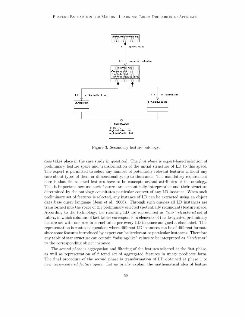
Feature Extraction for Machine Learning: Logic–Probabilistic Approach
Figure 3: Secondary feature ontology.
case takes place in the case study in question). The first phase is expert-based selection ofpreliminary feature space and transformation of the initial structure of LD to this space.The expert is permitted to select any number of potentially relevant features without anycare about types of them or dimensionality, up to thousands. The mandatory requirementhere is that the selected features have to be concepts or/and attributes of the ontology.This is important because such features are semantically interpretable and their structuredetermined by the ontology constitutes particular context of any LD instance. When suchpreliminary set of features is selected, any instance of LD can be extracted using an objectdata base query language (Jean et al., 2006). Through such queries all LD instances aretransformed into the space of the preliminary selected (potentially redundant) feature space.According to the technology, the resulting LD are represented as “star”-structured set oftables, in which columns of fact tables corresponds to elements of the designated preliminaryfeature set with one row in kernel table per every LD instance assigned a class label. Thisrepresentation is context-dependent where different LD instances can be of different formatssince some features introduced by expert can be irrelevant to particular instances. Thereforeany table of star structure can contain “missing-like” values to be interpreted as “irrelevant”to the corresponding object instance.
The second phase is aggregation and filtering of the features selected at the first phase,as well as representation of filtered set of aggregated features in unary predicate form.The final procedure of the second phase is transformation of LD obtained at phase 1 tonew class-centered feature space. Let us briefly explain the mathematical idea of feature
59
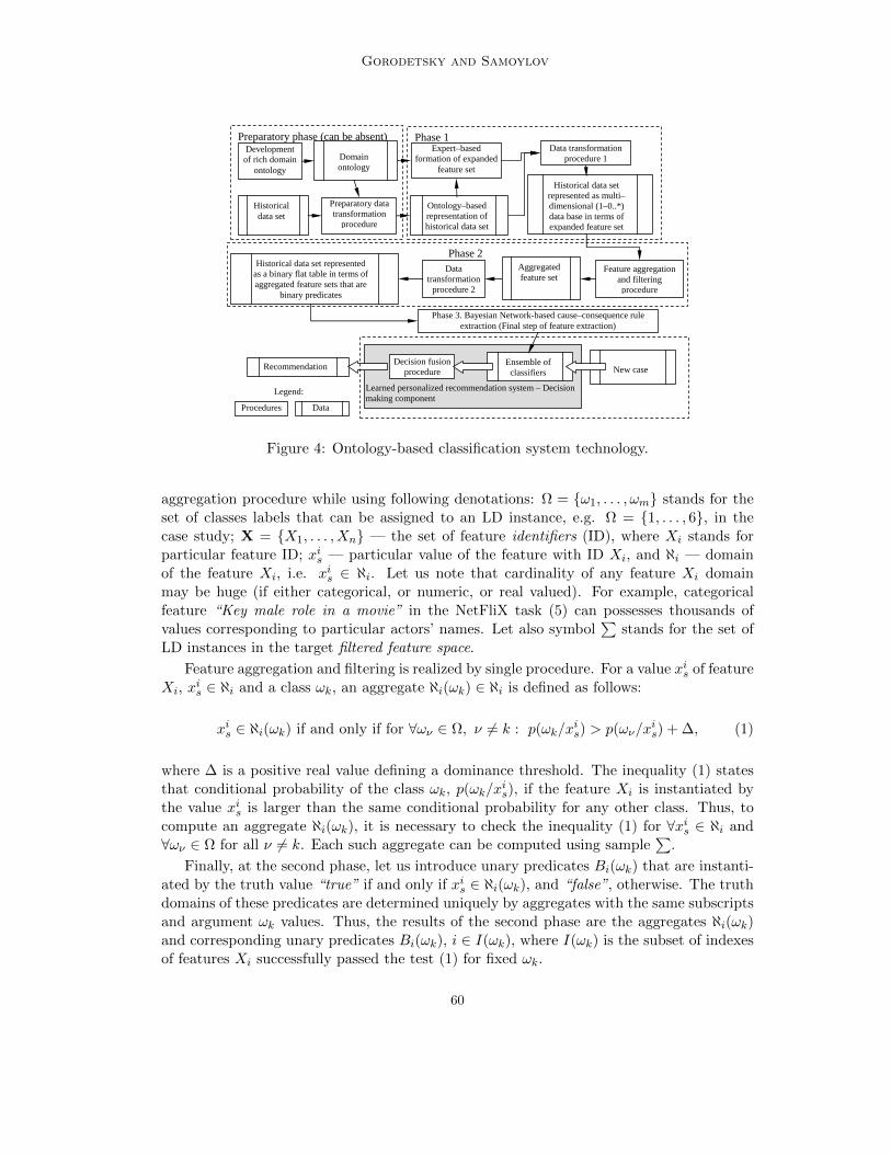
Gorodetsky and Samoylov
Phase 2
Phase 1
Historical data set represented as multi–dimensional (1–0..*) data base in terms of expanded feature set
Expert–based formation of expanded
feature set
Ontology–based representation of historical data set represented object
Preparatory phase (can be absent) Development of rich domain
ontology
Preparatory data transformation
procedure
Historical data set
Domain ontology
Data transformation procedure 1
Phase 3. Bayesian Network-based cause–consequence rule extraction (Final step of feature extraction)
Aggregated feature set
Feature aggregation and filtering procedure
Historical data set represented as a binary flat table in terms of aggregated feature sets that are
binary predicates
Data transformation
procedure 2
Recommendation
Legend:
Procedures Data
Learned personalized recommendation system – Decision making component
Ensemble of classifiers
Decision fusion procedure
New case
Figure 4: Ontology-based classification system technology.
aggregation procedure while using following denotations: Ω = ω1, . . . , ωm stands for theset of classes labels that can be assigned to an LD instance, e.g. Ω = 1, . . . , 6, in thecase study; X = X1, . . . , Xn — the set of feature identifiers (ID), where Xi stands forparticular feature ID; xi
s — particular value of the feature with ID Xi, and ℵi — domainof the feature Xi, i.e. xi
s ∈ ℵi. Let us note that cardinality of any feature Xi domainmay be huge (if either categorical, or numeric, or real valued). For example, categoricalfeature “Key male role in a movie” in the NetFliX task (5) can possesses thousands ofvalues corresponding to particular actors’ names. Let also symbol
∑stands for the set of
LD instances in the target filtered feature space.
Feature aggregation and filtering is realized by single procedure. For a value xis of feature
Xi, xis ∈ ℵi and a class ωk, an aggregate ℵi(ωk) ∈ ℵi is defined as follows:
xis ∈ ℵi(ωk) if and only if for ∀ων ∈ Ω, ν = k : p(ωk/xi
s) > p(ων/xis) + ∆, (1)
where ∆ is a positive real value defining a dominance threshold. The inequality (1) statesthat conditional probability of the class ωk, p(ωk/xi
s), if the feature Xi is instantiated bythe value xi
s is larger than the same conditional probability for any other class. Thus, tocompute an aggregate ℵi(ωk), it is necessary to check the inequality (1) for ∀xi
s ∈ ℵi and∀ων ∈ Ω for all ν = k. Each such aggregate can be computed using sample
∑.
Finally, at the second phase, let us introduce unary predicates Bi(ωk) that are instanti-ated by the truth value “true” if and only if xi
s ∈ ℵi(ωk), and “false”, otherwise. The truthdomains of these predicates are determined uniquely by aggregates with the same subscriptsand argument ωk values. Thus, the results of the second phase are the aggregates ℵi(ωk)and corresponding unary predicates Bi(ωk), i ∈ I(ωk), where I(ωk) is the subset of indexesof features Xi successfully passed the test (1) for fixed ωk.
60
Feature Extraction for Machine Learning: Logic–Probabilistic Approach
Using inequality (1) and definition of the predicates Bi(ωk), the LD sample∑
is trans-formed to the set of samples
∑(ω1), . . . ,
∑(ωm), representing LD in the space of binary
features that are predicates Bi(ωk).
The authors’ experience based on prototyping of several applications where the devel-oped technology was used showed that, as a rule, the procedure (1) filters many features ofthe set X1, . . . , Xn that are not satisfied with (1) for any ωk ∈ Ω. Let us also note thatthe value ∆ of the dominance threshold can be used as a means to restrict the total numberof the finally extracted features (either aggregates ℵi(ωk), or unary predicates Bi(ωk)) to apredefined limit.
Thus, in result of the phases 1 and 2 the source high dimensional heterogeneous LDof a complex structure is transformed to a homogeneous binary feature space of desirabledimension.
3.2 Cause-Consequence Rule Extraction
Phase 3 starts when aggregates ℵi(ωk), unary predicates Bi(ωk), i ∈ I(ωk), ωk ∈ Ω and LDsamples
∑(ω1), . . . ,
∑(ωm) are formed. In Fig. 4 this phase is denoted as phase 3. Its ob-
jective is to find cause-consequence dependencies (rules) between conjunction of predicatesBi(ωj), i ∈ I(ωj), Ω = ω1, . . . , ωm and ωj ∈ Ω. For this purpose, a probabilistic approachis used. Let us describe it for particular ωk ∈ Ω.
For ωk ∈ Ω probabilistic space is introduced as follows. The set of aggregates ℵi(ωj)is considered as a family set ℵi(ωj)|i∈I(ωk),j=1,...,m, where each set ℵi(ωj) is mapped aprobabilistic measure
p(ℵi(ωj)) = |ℵi(ωj)|/|ℵi|, (2)
where | | denotes cardinality of the corresponding set. It is clear that
p(Bi(ωj)) = p(ℵi(ωj)) (2′)
Since the aggregates ℵi(ωj) can overlap with ℵi(ωr), j = r these aggregates and correspond-ing random events can be dependent. Each set ℵi(ωj) of the family setℵi(ωj)|i∈I(ωk),j=1,...m, can also be correlated with any ωk ∈ Ω, which are also consid-ered in the model as random events with predefined a priory probabilities. Therefore thesets of family ωk|mk=1, ℵi(ωj)|i∈I(ωk),j=1,...m, cannot be used as elementary randomevents and thus probabilistic space cannot be defined here in the classical manner. In thiswork, “non-classical” definition of the probabilistic space and corresponding non-classicalprobability space axiomatics are used (Halpern, 2003).
While omitting some algebraic details, this probabilistic space projected to the subspacetaking into account only ωk can be modeled as an upper γ∨
k =< ωk, ℵi(ωj)|i∈I(ωk),j=1,...m,≥> or lower γ∧
k =< ωk, ℵi(ωj)|i∈I(ωk),j=1,...m, ≤> semi-lattice, where order relation isdefined in usual theoretic-set sense. In this semi-lattices, any node is mapped a probabilityof the corresponding random event. Further on, the lower semi-lattice is used. In this semi-lattice, ωk is the class label node called below “target node”. The model described below isidentical for any ωk ∈ Ω.
Definition. Hasse diagram of the lower semi-lattice γ∧k =< ωk, ℵi(ωj)|i∈I(ωk),j=1,...m,
≤> is below called Associative Bayesian Network (ABN).
61
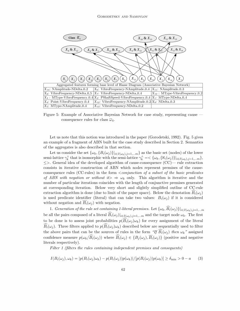
Gorodetsky and Samoylov
6X 7X3X 4X 5X1X 2X 14X12X
8X
128 & XX 138 & XX 1311 & XX
11X
1310 & XX
1413 & XX
1312 & XX
9X
139 & XX 1412 & XX
10X 14X
Class 4ω
13X
Aggregated features forming base level of Hasse Diagram (Associative Bayesian Network)
X14: NAmplitude-NDelta 0 2 X6: VibroFrequency-NAmplitude 0 4 X11: NAmplitude 0 3
X8: VibroFrequency-NDelta 0 5 X7: VibroFrequency-NDelta 0 4 X10 : MType-VibroFrequency 0 2
X3 : MType-VibroFrequency 0 4 X2: PShaftSpeed-VibroFrequency 0 4 X1: MType-NDelta 0 4
X4: Point-VibroFrequency 0 4 X12: VibroFrequency-NAmplitude 0 2 X9: NDelta 0 3
X5: MType-NAmplitude 0 4 X13: VibroFrequency-NDelta 0 2
Figure 5: Example of Associative Bayesian Network for case study, representing cause —consequence rules for class ω4.
Let us note that this notion was introduced in the paper (Gorodetski, 1992). Fig. 5 givesan example of a fragment of ABN built for the case study described in Section 2. Semanticsof the aggregates is also described in that section.
Let us consider the set ωk, Bi(ωj)|i∈I(ωk),j=1,...m as the basic set (nodes) of the lowersemi-lattice γ∧
k that is isomorphic with the semi-lattice γ∧k =< ωk, ℵi(ωj)|i∈I(ωk),j=1,...m,
≤>. General idea of the developed algorithm of cause-consequence (CC)— rule extractionconsists in iterative construction of ABN which nodes represent premises of the cause-consequence rules (CC-rules) in the form <conjunction of a subset of the basic predicatesof ABN with negation or without it> ⇒ ωk only. This algorithm is iterative and thenumber of particular iterations coincides with the length of conjunctive premises generatedat corresponding iteration. Below very short and slightly simplified outline of CC-ruleextraction algorithm is done (due to limit of the paper space). Below the denotation Bi(ωj)is used predicate identifier (literal) that can take two values: Bi(ωj) if it is consideredwithout negation and Bi(ωj) with negation.
1. Generation of the rule set containing 1-literal premises. Let ωk, Bi(ωj)|i∈I(ωk),j=1,...m
be all the pairs composed of a literal Bi(ωj)|i∈I(ωk),j=1,...m and the target node ωk. The first
to be done is to assess joint probabilities p(Bi(ωj)ωk) for every assignment of the literal
Bi(ωj). Three filters applied to p(Bi(ωj)ωk) described below are sequentially used to filter
the above pairs that can be the sources of rules in the form “If Bi(ωj) then ωk” assigned
confidence measure p(ωk/Bi(ωj)) where Bi(ωj) ∈ Bj(ωj), Bi(ωj) (positive and negativeliterals respectively).
Filter 1 (filters the rules containing independent premises and consequents)
I(Bi(ωj), ωk) = |p(Bi(ωj)ωk) − p(Bi(ωj))p(ωk)|/[p(Bi(ωj))p(ωk)] ≥ δmin > 0 − a (3)
62
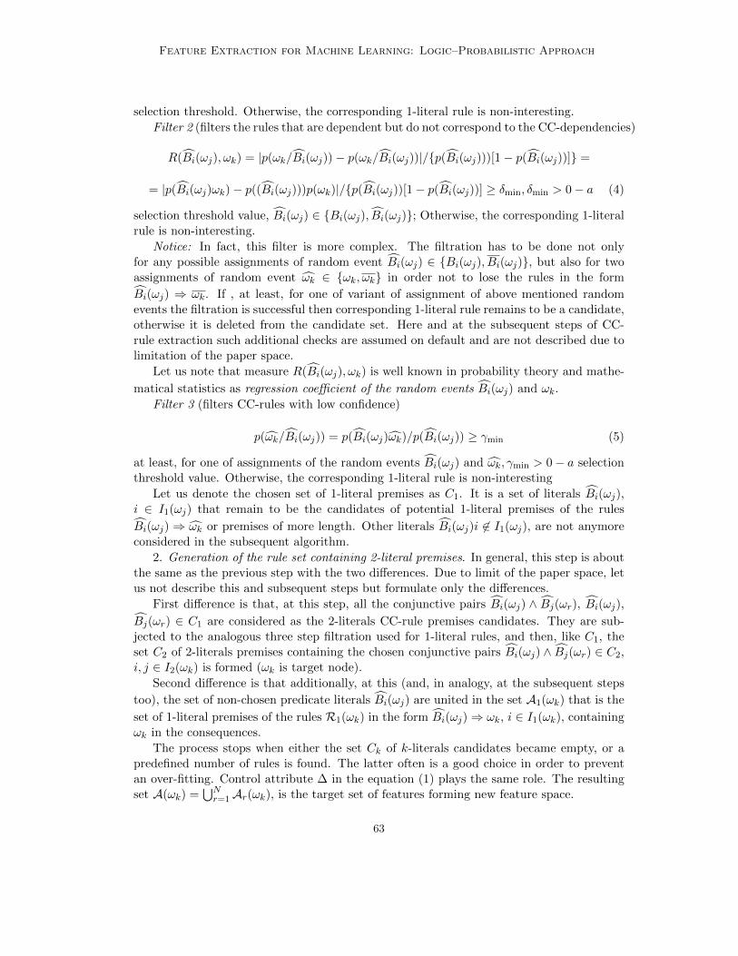
Feature Extraction for Machine Learning: Logic–Probabilistic Approach
selection threshold. Otherwise, the corresponding 1-literal rule is non-interesting.
Filter 2 (filters the rules that are dependent but do not correspond to the CC-dependencies)
R(Bi(ωj), ωk) = |p(ωk/Bi(ωj)) − p(ωk/Bi(ωj))|/p(Bi(ωj)))[1 − p(Bi(ωj))] =
= |p(Bi(ωj)ωk) − p((Bi(ωj)))p(ωk)|/p(Bi(ωj))[1 − p(Bi(ωj))] ≥ δmin, δmin > 0 − a (4)
selection threshold value, Bi(ωj) ∈ Bi(ωj), Bi(ωj); Otherwise, the corresponding 1-literalrule is non-interesting.
Notice: In fact, this filter is more complex. The filtration has to be done not onlyfor any possible assignments of random event Bi(ωj) ∈ Bi(ωj), Bi(ωj), but also for twoassignments of random event ωk ∈ ωk, ωk in order not to lose the rules in the form
Bi(ωj) ⇒ ωk. If , at least, for one of variant of assignment of above mentioned randomevents the filtration is successful then corresponding 1-literal rule remains to be a candidate,otherwise it is deleted from the candidate set. Here and at the subsequent steps of CC-rule extraction such additional checks are assumed on default and are not described due tolimitation of the paper space.
Let us note that measure R(Bi(ωj), ωk) is well known in probability theory and mathe-
matical statistics as regression coefficient of the random events Bi(ωj) and ωk.
Filter 3 (filters CC-rules with low confidence)
p(ωk/Bi(ωj)) = p(Bi(ωj)ωk)/p(Bi(ωj)) ≥ γmin (5)
at least, for one of assignments of the random events Bi(ωj) and ωk, γmin > 0 − a selectionthreshold value. Otherwise, the corresponding 1-literal rule is non-interesting
Let us denote the chosen set of 1-literal premises as C1. It is a set of literals Bi(ωj),i ∈ I1(ωj) that remain to be the candidates of potential 1-literal premises of the rules
Bi(ωj) ⇒ ωk or premises of more length. Other literals Bi(ωj)i ∈ I1(ωj), are not anymoreconsidered in the subsequent algorithm.
2. Generation of the rule set containing 2-literal premises. In general, this step is aboutthe same as the previous step with the two differences. Due to limit of the paper space, letus not describe this and subsequent steps but formulate only the differences.
First difference is that, at this step, all the conjunctive pairs Bi(ωj) ∧ Bj(ωr), Bi(ωj),
Bj(ωr) ∈ C1 are considered as the 2-literals CC-rule premises candidates. They are sub-jected to the analogous three step filtration used for 1-literal rules, and then, like C1, theset C2 of 2-literals premises containing the chosen conjunctive pairs Bi(ωj) ∧ Bj(ωr) ∈ C2,i, j ∈ I2(ωk) is formed (ωk is target node).
Second difference is that additionally, at this (and, in analogy, at the subsequent steps
too), the set of non-chosen predicate literals Bi(ωj) are united in the set A1(ωk) that is the
set of 1-literal premises of the rules R1(ωk) in the form Bi(ωj) ⇒ ωk, i ∈ I1(ωk), containingωk in the consequences.
The process stops when either the set Ck of k-literals candidates became empty, or apredefined number of rules is found. The latter often is a good choice in order to preventan over-fitting. Control attribute ∆ in the equation (1) plays the same role. The resultingset A(ωk) =
∪Nr=1 Ar(ωk), is the target set of features forming new feature space.
63
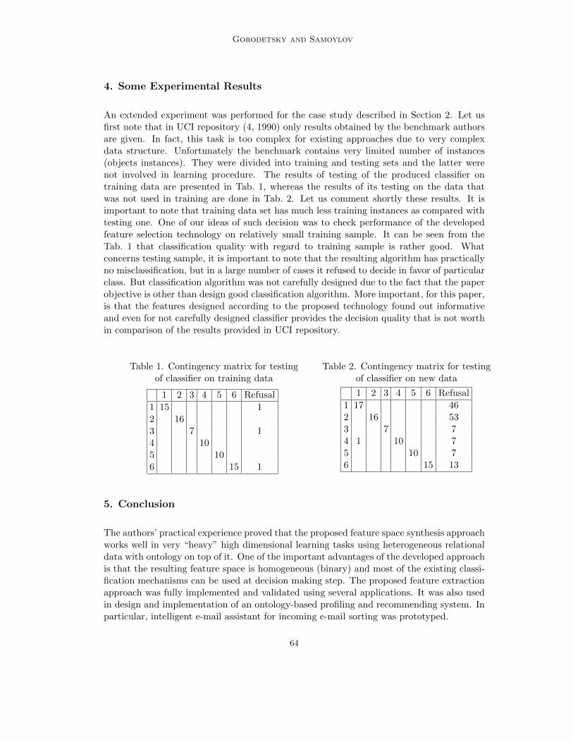
Gorodetsky and Samoylov
4. Some Experimental Results
An extended experiment was performed for the case study described in Section 2. Let usfirst note that in UCI repository (4, 1990) only results obtained by the benchmark authorsare given. In fact, this task is too complex for existing approaches due to very complexdata structure. Unfortunately the benchmark contains very limited number of instances(objects instances). They were divided into training and testing sets and the latter werenot involved in learning procedure. The results of testing of the produced classifier ontraining data are presented in Tab. 1, whereas the results of its testing on the data thatwas not used in training are done in Tab. 2. Let us comment shortly these results. It isimportant to note that training data set has much less training instances as compared withtesting one. One of our ideas of such decision was to check performance of the developedfeature selection technology on relatively small training sample. It can be seen from theTab. 1 that classification quality with regard to training sample is rather good. Whatconcerns testing sample, it is important to note that the resulting algorithm has practicallyno misclassification, but in a large number of cases it refused to decide in favor of particularclass. But classification algorithm was not carefully designed due to the fact that the paperobjective is other than design good classification algorithm. More important, for this paper,is that the features designed according to the proposed technology found out informativeand even for not carefully designed classifier provides the decision quality that is not worthin comparison of the results provided in UCI repository.
Table 1. Contingency matrix for testingof classifier on training data
1 2 3 4 5 6 Refusal
1 15 12 163 7 14 105 106 15 1
Table 2. Contingency matrix for testingof classifier on new data
1 2 3 4 5 6 Refusal
1 17 462 16 533 7 74 1 10 75 10 76 15 13
5. Conclusion
The authors’ practical experience proved that the proposed feature space synthesis approachworks well in very “heavy” high dimensional learning tasks using heterogeneous relationaldata with ontology on top of it. One of the important advantages of the developed approachis that the resulting feature space is homogeneous (binary) and most of the existing classi-fication mechanisms can be used at decision making step. The proposed feature extractionapproach was fully implemented and validated using several applications. It was also usedin design and implementation of an ontology-based profiling and recommending system. Inparticular, intelligent e-mail assistant for incoming e-mail sorting was prototyped.
64

Feature Extraction for Machine Learning: Logic–Probabilistic Approach
References
Netflix. http://www.netflix.com. different pruning measures can be used but this aspect isout of the paper scope.
Mechanical analysis data set, machine learning uci repository, 1990. URLhttp://archive.ics.uci.edu/ml/datasets/Mechanical+Analysis.
V. Gorodetski. Adaptation problems in expert systems. International Journal of AdaptiveControl and Signal Processing, 6:201–209, 1992.
J. Y. Halpern. Reasoning about uncertainty. MIT Press: Cambridge, 2003.
S. Jean, Y. Ait-Ameur, and G. Pierra. Querying ontology based database using ontoql (anontology query language). In LNCS, volume 4275, pages 704–721. Springer, 2006.
65
JMLR: Workshop and Conference Proceedings 10: 66-75 The Fourth Workshop on Feature Selection in Data Mining
Feature Extraction for Outlier Detection inHigh-Dimensional Spaces
Hoang Vu Nguyen [email protected]
Vivekanand Gopalkrishnan [email protected]
School of Computer Engineering
Nanyang Technological University
50 Nanyang Avenue, Singapore
Editor: Huan Liu, Hiroshi Motoda, Rudy Setiono, and Zheng Zhao
Abstract
This work addresses the problem of feature extraction for boosting the performance ofoutlier detectors in high-dimensional spaces. Recent years have observed the prominenceof multidimensional data on which traditional detection techniques usually fail to work asexpected due to the curse of dimensionality. This paper introduces an efficient feature ex-traction method which brings nontrivial improvements in detection accuracy when appliedon two popular detection techniques. Experiments carried out on real datasets demonstratethe feasibility of feature extraction in outlier detection.
Keywords: Feature Extraction, Dimensionality Reduction, Outlier Detection
1. Introduction
Outlier detection is an important data mining task and has been widely studied in recentyears (Knorr and Ng, 1998). As opposed to data clustering, where patterns representingthe majority are studied, anomaly or outlier detection aims at uncovering abnormal, rare,yet interesting knowledge which may stand for important events. Popular techniques foroutlier detection, especially distance-based ones (Knorr and Ng, 1998), usually computedistances of every data sample to its neighborhood to determine whether it is an outlier ornot. However, as these approaches compute distances in the full feature space, they sufferthe curse of dimensionality (Aggarwal and Yu, 2005).
Reducing data dimensions for better learning process, especially in sparsely filled high-dimensional spaces has been studied for a long time. Various solutions, ranging from prin-ciple component analysis (PCA) (Kirby and Sirovich, 1990), linear discriminant analysis(LDA) (Swets and Weng, 1996), null space LDA (NLDA) (Liu et al., 2004), etc., have beensuccessfully proposed to address this issue for the classification task. Outlier detection itselfcan be regarded as a binary asymmetric/unbalanced pattern classification problem, whereone class has much higher cardinality than the other, provided that some training data areavailable (Lazarevic and Kumar, 2005). Recently, Chawla et al. (2003) pointed out that thehigh imbalance in class cardinalities of asymmetric classification causes normal classificationtechniques to yield unsatisfactory accuracy (e.g., too complex learning rules which causeoverfitting). This necessitates the development of new techniques to specifically deal with
c⃝2010 Nguyen and Gopalkrishnan.

Feature Extraction for Outlier Detection
the issue. Analogously, existing feature extraction techniques for normal classification alsodo not work well when applied to our problem of interest. Particularly, Chen et al. (2008)highlights that traditional techniques typically seek accurate performance over a full rangeof instances, and hence, tend to classify all data into the majority class. This causes theminority class, which is usually more important, to be missed out. More suitable methods,like those in (Lee and Stolfo, 2000; Wu and Banzhaf, 2010), have been proposed to ad-dress the problem. In other words, it is impractical to apply standard discriminant featureextraction approaches for outlier detection.
In general, being able to reduce the number of data dimensions helps to overcome the lackof data and avoid the over-fitting issue. Recognizing this need, we present DimensionalityReduction/Feature Extraction for OUTlier Detection (DROUT), an efficient method forfeature extraction in outlier detection. In brief, DROUT first applies eigenspace regular-ization on a training set randomly sampled from the considered dataset. It then extractsa relevant set of features, and finally transforms the testing set where detection algorithmsare applied using the features obtained. By performing eigenspace regularization, we areable to mitigate the loss of discriminant information during the feature extraction process.Furthermore, different from other techniques on feature extraction, in DROUT, eigenvalueregularization and feature extraction are performed on weight-adjusted scatter matrices (ex-plained in Section 3) instead of normal ones. Those matrices specifically target at outlierdetection where class cardinalities (normal class v/s. outlier class) are highly unbalanced.This helps DROUT to work better than existing techniques in mining anomalies.
The rest of this paper is organized as follows. Related works are presented in the nextsection. We present the DROUT approach in Section 3. In Section 4, we apply DROUT ontwo existing outlier detection techniques and empirically evaluate its performance on realdatasets. Finally, we conclude the paper in Section 5 with directions for future work.
2. Literature Review
Linear subspace analysis for feature extraction and dimensionality reduction has been stud-ied in depth for a long time and many methods have been proposed in the literature,including principle component analysis (PCA) (Kirby and Sirovich, 1990), linear discrimi-nant analysis (LDA) (Swets and Weng, 1996), null space LDA (NLDA) (Liu et al., 2004)etc. Though applied very successfully for pattern classification, these methods usually missout some discriminant information while extracting relevant features for the classificationtask.
In particular, the eigenspace spanned by eigenvectors of the data within-class scattermatrix can be divided into three subspaces: the principal, the noise, and the null subspaces(Jiang et al., 2008). In words, the principal subspace, corresponding to eigenvectors of largeeigenvalues contains the most reliable discriminant information extracted from the trainingdata. The noise subspace, on the other hand is spanned by eigenvectors with nonzero smalleigenvalues. These eigenvalues are unreliable and cause over-fitting to each specific trainingset. Finally, the null subspace consists of eigenvectors of zero eigenvalues. The impact ofthe null subspace is similar to that of the noise one. Feature extraction methods typically:(a) solve the eigenvalue problem to obtain a set of eigenvectors and corresponding eigen-values, and (b) discard the unreliable dimensions with small eigenvalues and keep the rest
67

Nguyen and Gopalkrishnan
for performing the classification task. The noise and null subspaces are caused by noiseand mainly by the insufficient training data. As new data are added to the training setor as the training set is replaced by a different one, small or zero eigenvalues can be easilychanged, i.e., zero eigenvalues become nonzero and small ones become larger. Therefore,simply getting rid of them in the early stage may cause loss of discriminant information.This is especially true in the case of outlier detection because: (a) outliers are rare andhard to collect, (b) selecting subspaces for outlier detection is a complex problem (Aggar-wal and Yu, 2005). The second factor implies that outliers may be present in only somelower-dimensional projections of data. Thus, accidentally rejecting some dimensions just forthe sake of easy computation may lead to some loss of knowledge. Motivated by the issue,Jiang et al. (2008) proposes ERE, a dimensionality reduction method that first regularizesall three subspaces of the data within-class scatter matrix, and then extracts discriminantfeatures on the transformed total scatter matrix. The merit of ERE lies in the fact that nodimensionality reduction is done during the regularization phase, i.e. discriminant informa-tion is likely preserved.
Current solutions for feature extraction (including ERE) are unsuitable for binary asym-metric classification, because they rely on the usual within-class scatter matrix that afterbeing processed by solving the eigenvalue problem, usually leads to rejection of reliablefeatures. To overcome this issue, (Jiang, 2009) suggest to adjust the weights of class condi-tional covariance matrices. However, their proposed approach (APCDA) extracts discrim-inant features after applying PCA on the adjusted total scatter matrix. According to ouraforementioned discussion, this will cause loss of discriminant features.
3. The DROUT Approach
Our approach aims to overcome the weaknesses of the ERE and APCDA approaches. Simi-lar to APCDA, our DROUT approach performs eigenspace decomposition as well as featureextraction on the weight-adjusted scatter matrices. But in order to preserve the discrim-inant information till the feature extraction phase, DROUT applies the strategy of ERE,and does not discard any feature during the eigenspace regularization process. Thus, ourapproach can take advantage of both ERE and APCDA to overcome the curse of dimen-sionality in outlier detection.
In DROUT, the selected set of features is not a subset of the initial set of attributes, butis extracted from a transformation of the original data space (vector space). In order forDROUT to work, we make the following assumptions. First, a training set containing bothnormal data and a small amount of outliers is available. We further assume that trainingand testing sets have similar structures, allowing features extracted from the training setto be applicable on the testing set. While the latter assumption is widely used in almostall works on dimensionality reduction (Liu et al., 2004), the former appears frequently inworks on anomaly detection (Lazarevic and Kumar, 2005).
The training set in our assumption consists of two classes: the normal class ωm and theanomaly class ωa. The class ωm contains Nm points with class-conditional mean vector µm
and covariance matrix Σm. Analogously, Na, µa, and Σa are the support, class-conditionalmean vector, and covariance matrix of ωa. Each data point p is expressed as a column vectorof d dimensions, i.e., p ∈ Rd. Let Nt = Nm + Na be the training set’s total cardinality and
68
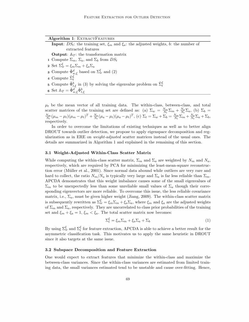
Feature Extraction for Outlier Detection
Algorithm 1: ExtractFeatures
Input: DSt: the training set, ξm and ξa: the adjusted weights, b: the number ofextracted features
Output: AT : the transformation matrixCompute Σm, Σa, and Σb from DSt1
Set Σξw = ξmΣm + ξaΣa2
Compute Φdw,ξ based on Σξ
w and (2)3
Compute Σξt4
Compute Φbt,ξ in (3) by solving the eigenvalue problem on Σξ
t5
Set AT = Φdw,ξΦ
bt,ξ6
µt be the mean vector of all training data. The within-class, between-class, and totalscatter matrices of the training set are defined as: (a) Σw = Nm
NtΣm + Na
NtΣa, (b) Σb =
NmNt
(µm − µt)(µm − µt)T + Na
Nt(µa − µt)(µa − µt)
T , (c) Σt = Σw + Σb = NmNt
Σm + NaNt
Σa + Σb,respectively.
In order to overcome the limitations of existing techniques as well as to better alignDROUT towards outlier detection, we propose to apply eigenspace decomposition and reg-ularization as in ERE on weight-adjusted scatter matrices instead of the usual ones. Thedetails are summarized in Algorithm 1 and explained in the remaining of this section.
3.1 Weight-Adjusted Within-Class Scatter Matrix
While computing the within-class scatter matrix, Σm and Σa are weighted by Nm and Na,respectively, which are required by PCA for minimizing the least-mean-square reconstruc-tion error (Muller et al., 2001). Since normal data abound while outliers are very rare andhard to collect, the ratio Nm/Na is typically very large and Σa is far less reliable than Σm.APCDA demonstrates that this weight imbalance causes some of the small eigenvalues ofΣm to be unexpectedly less than some unreliable small values of Σa though their corre-sponding eigenvectors are more reliable. To overcome this issue, the less reliable covariancematrix, i.e., Σa, must be given higher weight (Jiang, 2009). The within-class scatter matrix
is subsequently rewritten as Σξw = ξmΣm + ξaΣa, where ξm and ξa are the adjusted weights
of Σm and Σa, respectively. They are uncorrelated to class prior probabilities of the trainingset and ξm + ξa = 1, ξm < ξa. The total scatter matrix now becomes:
Σξt = ξmΣm + ξaΣa + Σb (1)
By using Σξw and Σξ
t for feature extraction, APCDA is able to achieve a better result for theasymmetric classification task. This motivates us to apply the same heuristic in DROUTsince it also targets at the same issue.
3.2 Subspace Decomposition and Feature Extraction
One would expect to extract features that minimize the within-class and maximize thebetween-class variances. Since the within-class variances are estimated from limited train-ing data, the small variances estimated tend to be unstable and cause over-fitting. Hence,
69
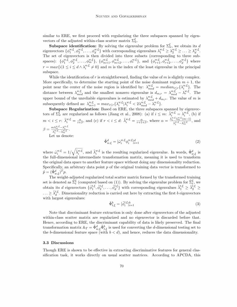
Nguyen and Gopalkrishnan
similar to ERE, we first proceed with regularizing the three subspaces spanned by eigen-vectors of the adjusted within-class scatter matrix Σξ
w.
Subspace identification: By solving the eigenvalue problem for Σξw, we obtain its d
eigenvectors ϕw,ξ1 , ϕw,ξ
2 , . . . , ϕw,ξd with corresponding eigenvalues λw,ξ
1 ≥ λw,ξ2 ≥ . . . ≥ λw,ξ
d .The set of eigenvectors is then divided into three subsets (corresponding to three sub-
spaces): ϕw,ξ1 , ϕw,ξ
2 , . . . , ϕw,ξm , ϕw,ξ
m+1, ϕw,ξm+2, . . . , ϕ
w,ξr , and ϕw,ξ
r+1, ϕw,ξr+2, . . . , ϕ
w,ξd where
r = maxi|1 ≤ i ≤ d ∧ λw,ξi = 0 and m is the index of the least eigenvalue in the principal
subspace.
While the identification of r is straightforward, finding the value of m is slightly complex.More specifically, to determine the starting point of the noise dominant region m + 1, thepoint near the center of the noise region is identified by: λw,ξ
med = mediani≤rλw,ξi . The
distance between λw,ξmed and the smallest nonzero eigenvalue is dm,r = λw,ξ
med − λw,ξr . The
upper bound of the unreliable eigenvalues is estimated by λw,ξmed + dm,r. The value of m is
subsequently defined as: λw,ξm+1 = maxi≤rλw,ξ
i |λw,ξi < 2λw,ξ
med − λw,ξr .
Subspace Regularization: Based on ERE, the three subspaces spanned by eigenvec-tors of Σξ
w are regularized as follows (Jiang et al., 2008): (a) if i ≤ m: λw,ξi = λw,ξ
i , (b) if
m < i ≤ r: λw,ξi = α
i+β , and (c) if r < i ≤ d: λw,ξi = α
r+1+β , where α =λw,ξ1 λw,ξ
m (m−1)
λw,ξ1 −λw,ξ
m, and
β =mλw,ξ
m −λw,ξ1
λw,ξ1 −λw,ξ
m.
Let us denote:
Φdw,ξ = [ωw,ξ
i ϕw,ξi ]di=1 (2)
where ωw,ξi = 1/
√λw,ξ
i , and λw,ξi is the resulting regularized eigenvalue. In words, Φd
w,ξ isthe full-dimensional intermediate transformation matrix, meaning it is used to transformthe original data space to another feature space without doing any dimensionality reduction.Specifically, an arbitrary data point p of the original training data vector is transformed top = (Φd
w,ξ)T p.
The weight-adjusted regularized total scatter matrix formed by the transformed trainingset is denoted as Σξ
t (computed based on (1)). By solving the eigenvalue problem for Σξt , we
obtain its d eigenvectors ϕt,ξ1 , ϕt,ξ
2 , . . . , ϕt,ξd with corresponding eigenvalues λt,ξ
1 ≥ λt,ξ2 ≥
. . . ≥ λt,ξd . Dimensionality reduction is carried out here by extracting the first b eigenvectors
with largest eigenvalues:
Φbt,ξ = [ϕt,ξ
i ]bi=1 (3)
Note that discriminant feature extraction is only done after eigenvectors of the adjustedwithin-class scatter matrix are regularized and no eigenvector is discarded before that.Hence, according to ERE, the discriminant capability of data is likely preserved. The finaltransformation matrix AT = Φd
w,ξΦbt,ξ is used for converting the d-dimensional testing set to
the b-dimensional feature space (with b < d), and hence, reduces the data dimensionality.
3.3 Discussions
Though ERE is shown to be effective in extracting discriminative features for general clas-sification task, it works directly on usual scatter matrices. According to APCDA, this
70
Feature Extraction for Outlier Detection
is irrelevant for asymmetric classification. In particular, the less reliable covariance ma-trix corresponding to the rare class (i.e., the class of anomalies) must be assigned higherweight. Though APCDA adjusts the scatter matrices for the feature extraction task, itstarts extracting features at the eigenvalue regularization stage, which causes a loss in dis-criminant power (Jiang et al., 2008). The topic of dimensionality reduction for asymmetricclassification is also explored in (Lindgren and Spangeus, 2004). Their technique, ACP,measures the spread of class ωa with respect to ωm’s mean rather than to that of ωa itself.It then solves the following generalized eigenvalue problem to extract discriminant features:ΣaD = ΣmDΛ, where (a) Σa is the modified version of Σa, (b) Λ, DT ΣmD, and DT ΣaD arediagonal. However, ACP neither considers the issue of imbalanced class cardinalities, northe importance of the noise and null subspaces. As a consequence, ACP does not performwell for outlier detection (c.f., empirical evaluation in Section 4).
Combining the findings in both ERE and APCDA, we perform eigenspace decomposi-tion and feature extraction on the weight-adjusted scatter matrices. The weights assignedhere are unrelated to the class prior probabilities. This allows us to benefit from both fea-ture extraction techniques for overcoming the curse of dimensionality in outlier detection.APCDA suggests to set ξm = 0.2 and ξa = 0.8. However, in outlier detection, the numberof normal data points are expected to be much larger than anomalies. Hence we proposeto use ξm = 0.1 and ξa = 0.9 with asymmetric ratio ξa/ξm = 9. In other words, we expectoutliers to occupy only up to 10% of the total dataset’s size. This agrees with many pre-vious studies (Angiulli and Fassetti, 2009; Lazarevic and Kumar, 2005). In this paper aswell as in other these works, the number of outliers in an arbitrary dataset is assumed tobe much less than 10% of the dataset’s cardinality (e.g., 1% or 5%). Nonetheless, we findthat setting the asymmetric ratio to 9 is good enough for practical applications, though agood performance is achieved even with larger values.
The runtime cost of DROUT is O(Ntd·min(Nt, d)), which is comparable to other featureextraction techniques (Swets and Weng, 1996). However, since DROUT is only performedonce on a small training set, this time complexity is not that important. Instead, theruntime overhead of the testing phase which is executed on a much larger dataset is of ourgreat interest. Note that running detection methods on a transformed testing set will costless time than on a full-dimensional one since their runtime overheads are proportional tothe number of dimensions (Angiulli and Fassetti, 2009).
4. Outlier Detection with DROUT
In this section, we demonstrate the benefit of applying DROUT on two popular outlierdetection techniques, through experiments on real datasets.
4.1 Detection Techniques
ORCA: In the field of distance-based outlier detection, ORCA (Bay and Schwabacher,2003) is one of the most popular methods due to its high efficiency in terms of time com-plexity and accuracy. In ORCA, we aim to detect top n outliers whose total distances totheir respective k nearest neighbors are largest. Since its outlier definition is based on thenotion of nearest neighbors, and we know that nearest and farthest neighbors are roughlythe same in such spaces (Aggarwal and Yu, 2005), ORCA suffers the curse of dimensionality
71
Nguyen and Gopalkrishnan
(i.e. its accuracy is reduced in high-dimensional spaces).
BSOUT: Kollios et al. (2003) introduces Biased Sampling OUTlier Detection (BSOUT)which aims to flag outliers whose total numbers of neighbors within radius R (called R-neighborhood) are less than a threshold P . In BSOUT, each data point p’s local densityis first estimated using a nonparametric kernel density estimator. Its R-neighborhood’scardinality is then approximated based on the calculated density. If this amount falls belowP , it is placed in the candidate set which will be refined later to obtain true outliers. Similarto ORCA, the performance of BSOUT also degrades in high-dimensional data because oftwo reasons. While the first reason is analogous to ORCA’s, the second one stems from thefact that BSOUT utilizes nonparametric density estimation, and it is known that estimationaccuracy downgrades greatly in such data (Muller et al., 2001).
4.2 Experiment Setup
Testing Procedure: We evaluate the performance of DROUT, ERE, APCDA, and ACP(Lindgren and Spangeus, 2004) when applying to ORCA and BSOUT. The detection ac-curacy here is measured as the area under the ROC curve, called AUC, which is widelyused to assess outlier detectors. We compare the performance of ORCA and BSOUT onthe original set of attributes, against ORCA on the new feature set obtained by applyingeach of the dimensionality reduction techniques. In order to use AUC as the evaluationmetric, we employ real datasets that can be converted to the binary classification problem.This setup procedure has been successfully used for studying outlier detection (Lazarevicand Kumar, 2005).
Benchmark Datasets: The first dataset is extracted from the KDD Cup 1999 one fol-lowing the method introduced in (Lazarevic and Kumar, 2005). Particularly, the smallestintrusion class, U2R, consisting of 246 data points is selected as the outlier class ωa. Thisclass contains a variety types of attacks like ftp write, imap, multihop, nmap, phf, pod,and teardrop. The total dataset hence includes the normal class ωm of 60593 data recordsand 246 outliers in d-dimensional space with d = 34 (we have excluded the 7 categoricalattributes from the total of 41 attributes). The second dataset, Ann-Thyroid, is taken fromthe UCI Machine Learning Repository. It contains 3428 records in 21-dimensional space.The largest class (class 3) is selected as the normal class ωm, and we generate two test sets:Ann-Thyroid 1 (ωa is class 1), and Ann-Thyroid 2 (ωa is class 2). The maximum datasetdimensionality in our experiment is 34 which is similar to that of (Aggarwal and Yu, 2005).
4.3 Results
With the KDD dataset, we randomly sample 50 records from ωa and 1000 records from ωm
for training, and keep the remaining 59789 records for testing. For the Ann-Thyroid dataset,we randomly select 50 records from ωa and 450 records from ωm for training, and keep theremaining (2751 records for Ann-Thyroid 1, and 2855 for Ann-Thyroid 2) for testing. Noticethat the asymmetric ratio is 20 and 9 for the KDD and Ann-Thyroid datasets, respectively.This means our approach’s performance is also assessed in the case the asymmetric ratio isnot exactly 9.
72
Feature Extraction for Outlier Detection
1 2 4 6 8 10 12 14 16 170.4
0.5
0.6
0.7
0.8
0.9
1
Number of Extracted Features (b)
AU
CORCAAPCDAACPEREDROUT
(a) KDD Cup 1999
1 2 4 6 8 100.4
0.5
0.6
0.7
0.8
0.9
1
Number of Extracted Features (b)
AU
C
ORCAAPCDAACPEREDROUT
(b) Ann-Thyroid 1
1 2 4 6 8 100.4
0.5
0.6
0.7
0.8
0.9
1
Number of Extracted Features (b)
AU
C
ORCAAPCDAACPEREDROUT
(c) Ann-Thyroid 2
Figure 1: Effect of feature extraction techniques on accuracy of ORCA.
For ORCA, the number of nearest neighbors k is varied in the range 0.02%N ≤ k ≤0.1%N with N being the underlying dataset’s size, while n is chosen to be 0.05%N . WithBSOUT, P is also varied from 0.02%N to 0.1%N and R is chosen such that the numberof outliers flagged using the algorithm in (Knorr and Ng, 1998) is exactly 0.05%N . Theseparameter settings follow the proposal in previous work (Angiulli and Fassetti, 2009). Foreach value of b (number of extracted features) tested (b ≤ ⌊d/2⌋), we construct the trainingset using random split described above for five times. The resultant average AUCs andtheir respective standard deviations are computed. Since the values of standard deviationsare negligible, we do not present them in our results.
Dimensionality Reduction on ORCA: Figure 1 describes how the AUC values of ORCAusing different dimensionality reduction methods change as b increases. Notice that the per-formance of the original ORCA is unrelated to b. With small values of b, ORCA with featureextraction performs worse than the original ORCA. This is because by using insufficientnumber of features, discriminant information is likely lost even though the extraction pro-cess has been carefully designed to preserve it. However, for higher values of b, featureextraction starts producing better accuracy. The performance of APCDA is slightly betterthan ERE in general while ACP loses out in all test cases. On the other hand, DROUTachieves the best accuracy and highest gain in detection quality attributed to the fact thatit performs dimensionality reduction on the adjusted scatter matrices and no feature re-jection is carried out during the eigenspace regularization process. Overall, increasing bdoes not ensure a better detection accuracy for methods utilizing feature extraction. Thisis reflected by a slight reduction and then relative stabilization of the AUC curves. Theoutcomes suggest that b should not be too large (e.g., b ≤ ⌊d/2⌋), otherwise the curse ofdimensionality will happen again on the new feature space.
Dimensionality Reduction on BSOUT: From Figure 2, it can be seen that withBSOUT, the performance gain by applying feature extraction is even more pronounced.This is because, as compared to ORCA, BSOUT has one more factor causing its accuracyto downgrade in high-dimensional spaces: the nonparametric kernel density estimation.Therefore, reducing dimensions in BSOUT brings two benefits, it: (a) makes the notion ofnearest neighbors more meaningful, and (b) improves the accuracy of estimating data localdensities. Among the feature extraction techniques utilized, DROUT once again yields the
73
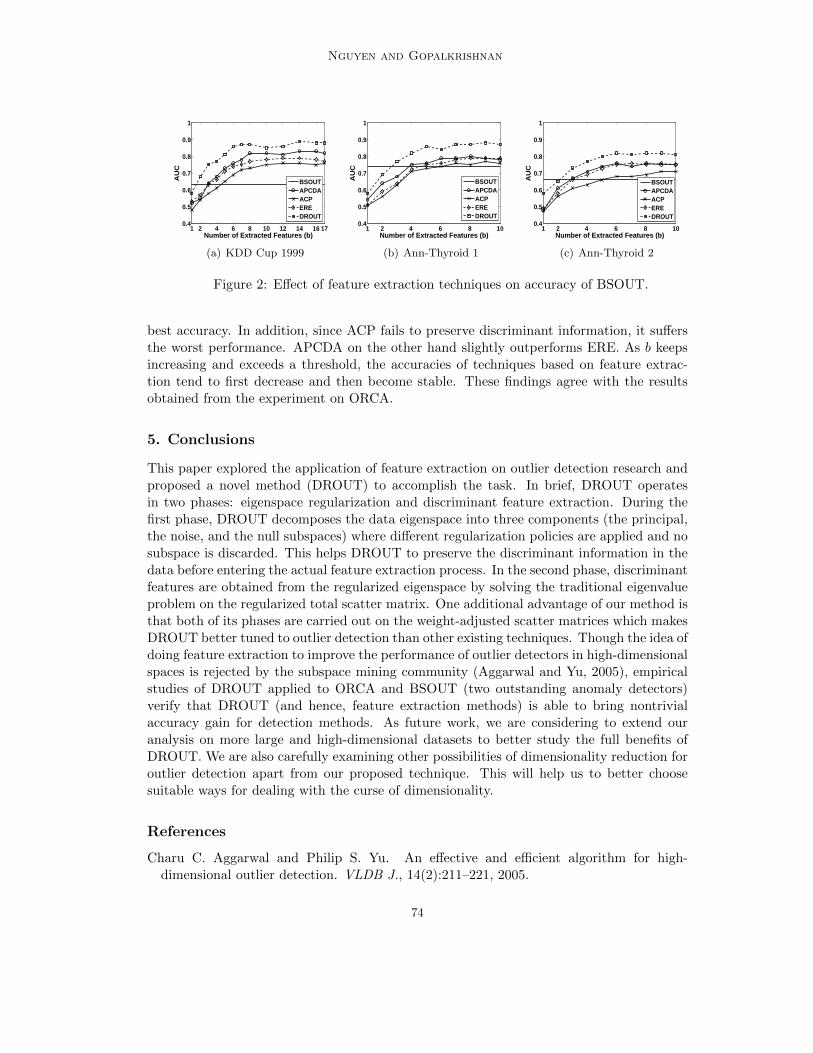
Nguyen and Gopalkrishnan
1 2 4 6 8 10 12 14 16 170.4
0.5
0.6
0.7
0.8
0.9
1
Number of Extracted Features (b)
AU
CBSOUTAPCDAACPEREDROUT
(a) KDD Cup 1999
1 2 4 6 8 100.4
0.5
0.6
0.7
0.8
0.9
1
Number of Extracted Features (b)
AU
C
BSOUTAPCDAACPEREDROUT
(b) Ann-Thyroid 1
1 2 4 6 8 100.4
0.5
0.6
0.7
0.8
0.9
1
Number of Extracted Features (b)
AU
C
BSOUTAPCDAACPEREDROUT
(c) Ann-Thyroid 2
Figure 2: Effect of feature extraction techniques on accuracy of BSOUT.
best accuracy. In addition, since ACP fails to preserve discriminant information, it suffersthe worst performance. APCDA on the other hand slightly outperforms ERE. As b keepsincreasing and exceeds a threshold, the accuracies of techniques based on feature extrac-tion tend to first decrease and then become stable. These findings agree with the resultsobtained from the experiment on ORCA.
5. Conclusions
This paper explored the application of feature extraction on outlier detection research andproposed a novel method (DROUT) to accomplish the task. In brief, DROUT operatesin two phases: eigenspace regularization and discriminant feature extraction. During thefirst phase, DROUT decomposes the data eigenspace into three components (the principal,the noise, and the null subspaces) where different regularization policies are applied and nosubspace is discarded. This helps DROUT to preserve the discriminant information in thedata before entering the actual feature extraction process. In the second phase, discriminantfeatures are obtained from the regularized eigenspace by solving the traditional eigenvalueproblem on the regularized total scatter matrix. One additional advantage of our method isthat both of its phases are carried out on the weight-adjusted scatter matrices which makesDROUT better tuned to outlier detection than other existing techniques. Though the idea ofdoing feature extraction to improve the performance of outlier detectors in high-dimensionalspaces is rejected by the subspace mining community (Aggarwal and Yu, 2005), empiricalstudies of DROUT applied to ORCA and BSOUT (two outstanding anomaly detectors)verify that DROUT (and hence, feature extraction methods) is able to bring nontrivialaccuracy gain for detection methods. As future work, we are considering to extend ouranalysis on more large and high-dimensional datasets to better study the full benefits ofDROUT. We are also carefully examining other possibilities of dimensionality reduction foroutlier detection apart from our proposed technique. This will help us to better choosesuitable ways for dealing with the curse of dimensionality.
References
Charu C. Aggarwal and Philip S. Yu. An effective and efficient algorithm for high-dimensional outlier detection. VLDB J., 14(2):211–221, 2005.
74
Feature Extraction for Outlier Detection
Fabrizio Angiulli and Fabio Fassetti. Dolphin: An efficient algorithm for mining distance-based outliers in very large datasets. TKDD, 3(1), 2009.
Stephen D. Bay and Mark Schwabacher. Mining distance-based outliers in near linear timewith randomization and a simple pruning rule. In KDD, pages 29–38, 2003.
Nitesh V. Chawla, Aleksandar Lazarevic, Lawrence O. Hall, and Kevin W. Bowyer.SMOTEBoost: Improving prediction of the minority class in boosting. In PKDD, pages107–119, 2003.
Mu-Chen Chen, Long-Sheng Chen, Chun-Chin Hsu, and Wei-Rong Zeng. An informationgranulation based data mining approach for classifying imbalanced data. Inf. Sci., 178(16):3214–3227, 2008.
Xudong Jiang. Asymmetric principal component and discriminant analyses for patternclassification. IEEE Trans. Pattern Anal. Mach. Intell., 31(5), 2009.
Xudong Jiang, Bappaditya Mandal, and Alex ChiChung Kot. Eigenfeature regularizationand extraction in face recognition. IEEE Trans. Pattern Anal. Mach. Intell., 30(3):383–394, 2008.
M. Kirby and L. Sirovich. Application of the karhunen-loeve procedure for the characteri-zation of human faces. IEEE Trans. Pattern Anal. Mach. Intell., 12(1):103–108, 1990.
Edwin M. Knorr and Raymond T. Ng. Algorithms for mining distance-based outliers inlarge datasets. In VLDB, pages 392–403, 1998.
George Kollios, Dimitrios Gunopulos, Nick Koudas, and Stefan Berchtold. Efficient biasedsampling for approximate clustering and outlier detection in large data sets. IEEE Trans.Knowl. Data Eng., 15(5):1170–1187, 2003.
Aleksandar Lazarevic and Vipin Kumar. Feature bagging for outlier detection. In KDD,pages 157–166, 2005.
Wenke Lee and Salvatore J. Stolfo. A framework for constructing features and models forintrusion detection systems. ACM Trans. Inf. Syst. Secur., 3(4):227–261, 2000.
David Lindgren and Per Spangeus. A novel feature extraction algorithm for asymmetricclassification. IEEE Sensors Journal, 4(5):643–650, 2004.
Wei Liu, Yunhong Wang, Stan Z. Li, and Tieniu Tan. Null space approach of fisher dis-criminant analysis for face recognition. In ECCV Workshop BioAW, pages 32–44, 2004.
Klaus-Robert Muller, Sebastian Mika, Gunnar Ratsch, Koji Tsuda, and BernhardScholkopf. An introduction to kernel-based learning algorithms. IEEE Transactionson Neural Networks, 12(2):181–201, 2001.
Daniel L. Swets and Juyang Weng. Using discriminant eigenfeatures for image retrieval.IEEE Trans. Pattern Anal. Mach. Intell., 18(8):831–836, 1996.
Shelly Xiaonan Wu and Wolfgang Banzhaf. The use of computational intelligence in intru-sion detection systems: A review. Applied Soft Computing, 10(1):1–35, 2010.
75
JMLR: Workshop and Conference Proceedings 10: 76-85 The Fourth Workshop on Feature Selection in Data Mining
Feature Selection for Text Classification Based onGini Coefficient of Inequality
Sanasam Ranbir Singh [email protected] of Computer Science and EngineeringIndian Institute of Technology GuwahatiGuwahati 781039, Assam, India
Hema A. Murthy [email protected] of Computer Science and EngineeringIndian Institute of Technology MadrasChannai 600036, Tamil Nadu, India.
Timothy A. Gonsalves [email protected]
Department of Computer Science and Engineering
Indian Institute of Technology Madras
Channai 600036, Tamil Nadu, India
Editor: Huan Liu, Hiroshi Motoda, Rudy Setiono, and Zheng Zhao
Abstract
A number of feature selection mechanisms have been explored in text categorization, amongwhich mutual information, information gain and chi-square are considered most effective. Inthis paper, we study another method known as within class popularity to deal with featureselection based on the concept Gini coefficient of inequality (a commonly used measureof inequality of income). The proposed measure explores the relative distribution of afeature among different classes. From extensive experiments with four text classifiers overthree datasets of different levels of heterogeneity, we observe that the proposed measureoutperforms the mutual information, information gain and chi-square static with an averageimprovement of approximately 28.5%, 19% and 9.2% respectively.
Keywords: Text categorization, feature selection, gini coefficient, within class popularity
1. Introduction
Text categorization (TC) is a supervised learning problem where the task is to assign a giventext document to one or more predefined categories. It is a well-studied problem and stillcontinues to be topical area in information retrieval (IR), because of the ever increasingamount of easily accessible digital documents on the Web, and, the necessity for organisedand effective retrieval. High dimensionality of feature space is a major problem in TC. Thenumber of terms (i.e., features) present in a collection of documents, in general, is large andfew are informative. Feature selection for TC is the task of reducing dimensionality of featurespace by identifying informative features and its primary goals are improving classificationeffectiveness, computational efficiency, or both. The performance of a classifier is affectedby the employed feature selection mechanism.
c⃝2010 Singh, Murthy and Gonsalves.

Feature Selection for Text Classification Based on Gini Coefficient of Inequality
This paper proposes a feature selection mechanism called within class popularity (WCP)which addresses two improtant issues of feature selection for text classification i.e., unevendistribution of prior class probability and global goodness of a feature. The performanceof WCP is then compared with the performance of the most commonly used measures –mutual information (MI), information gain(IG), chi-square(CHI).
The rest of the paper is organised as follows. Section 2 reviews few related studies. Sec-tion 3 presents the proposed feature selection. Section 4 presents experimental evaluations.The paper concludes in Section 5.
2. Review of Few Related Studies
At present feature selection methods for TC are based on statistical theory and machinelearning. Some well-known methods are information gain, term frequency, mutual informa-tion, chi-square statics, Gini index (Yang and Pedersen, 1997; Shankar and Karypis, 2000).We briefly review these measures in this section.
2.1 Mutual Information:
Mutual information (MI) between a term t and a class c is defined by MI(t, c) = log Pr(t,c)Pr(t)Pr(c) .
To measure the global goodness of a term in feature selection, we combine the categoryspecific scores as MImax(t) = maxi MI(t, ci). Alternatively, in some studies (Yang andPedersen, 1997), it is also define as MImax(t) =
∑i Pr(ci)MI(t, ci).
2.2 Information Gain:
It is defined by following expression (Yang and Pedersen, 1997).
IG(t) = −∑i Pr(ci) log Pr(ci) + Pr(t)
∑i Pr(ci|t) log Pr(ci|t)
+Pr(t)∑
i Pr(ci|t) log Pr(ci|t)
It is frequently used as a term goodness criterion in machine learning. It measures thenumber of bits required for category prediction by knowing the presence or the absence ofa term in the document.
2.3 χ2 static:
The χ2 static (CHI) is defined by the following expression (Yang and Pedersen, 1997).
χ2(t, c) =N × (AD − CB)2
(A + C) × (B + D) × (A + B) × (C + D)
where N is the number of documents, A is the number of documents of class c containing theterm t, B is the number of documents of other class (not c) containing t, C is the number ofdocuments of class c not containing the term t and D is the number of documents of otherclass not containing t. It measures the lack of independence between t and c and compa-rable to χ2 distribution with one degree of freedom. The commonly used global goodnessestimation functions are maximum and mean functions i.e.,χ2(f) = arg maxci χ2(f, ci) orχ2(f) =
∑i Pr(ci)χ
2(f, ci).
77
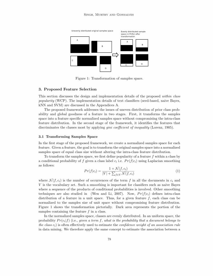
Singh, Murthy and Gonsalves
Figure 1: Transformation of samples space.
3. Proposed Feature Selection
This section discusses the design and implementation details of the proposed within classpopularity (WCP). The implementation details of text classifiers (seed-based, naive Bayes,kNN and SVM) are discussed in the Appendices A.
The proposed framework addresses the issues of uneven distribution of prior class prob-ability and global goodness of a feature in two stages. First, it transforms the samplesspace into a feature specific normalized samples space without compromising the intra-classfeature distribution. In the second stage of the framework, it identifies the features thatdiscriminates the classes most by applying gini coefficient of inequality (Lorenz, 1905).
3.1 Transforming Samples Space
In the first stage of the proposed framework, we create a normalized samples space for eachfeature. Given a feature, the goal is to transform the original samples space into a normalizedsamples space of equal class size without altering the intra-class feature distribution.
To transform the samples space, we first define popularity of a feature f within a class bya conditional probability of f given a class label ci i.e. Pr(f |ci) using Laplacian smoothingas follows:
Pr(f |ci) =1 + N (f, ci)
|V | +∑
f∈V N (f, ci)(1)
where N (f, ci) is the number of occurrences of the term f in all the documents in ci andV is the vocabulary set. Such a smoothing is important for classifiers such as naive Bayeswhere a sequence of the products of conditional probabilities is involved. Other smoothingtechniques are also studied in (Wen and Li, 2007). Now, Pr(f |ci) defines intra-classdistribution of a feature in a unit space. Thus, for a given feature f , each class can benormalized to the samples size of unit space without compromising feature distribution.Figure 1 shows the transformation pictorially. Dark area represents the portion of thesamples containing the feature f in a class.
In the normalized samples space, classes are evenly distributed. In an uniform space, theprobability Pr(ci|f) (i.e., given a term f , what is the probability that a document belongs tothe class ci) is often effectively used to estimate the confidence weight of an association rulein data mining. We therefore apply the same concept to estimate the association between a
78

Feature Selection for Text Classification Based on Gini Coefficient of Inequality
A
B
Cumulative share of population from lowest to highest (%)
Cumulat iveshare of income (%)
100%
100%
Line of equality
Lorenz curve
Figure 2: (a) Graphical representation of the Gini index coefficient.
class and a feature. We now normalize the above popularity weight (i.e. Equation 1) acrossall classes and define within class popularity as follows.
wcp(f, ci) =Pr(f |ci)∑|C|
k=1 Pr(f |ck)(2)
where C is the set of the class labels. It has the following characteristics:
• ∑i wcp(f, ci) = 1.
• wcp(f, ci) ranges between (0, 1) i.e., 0 < wcp(f, ci) < 1. It is because Pr(f |ci) > 0.
• if a term f is evenly distributed across all classes then wcp(f, ci) = 1/|C|∀ci ∈ C.
• if wcp(f, ci) > wcp(f, cj), then feature f is present more densely in the class ci thanclass cj .
• if wcp(f, ci) ≈ 1, then the feature f is likely to be present only in the class ci.
Remark 1 The wcp(f, ci) is equivalent to Pr(ci|f) in the normalized samples space. Sincethe classes are evenly distributed in the normalized samples space, wcp(f, ci) is un-biased toprior class probability.
As effectively used in association rules mining, with a reasonably high support weight (i.e.,Pr(f |ci)), a high value of wcp(f, ci) can represent high association between a class and afeature.
A conceptually similar feature selector has been used in (Aggarwal et al., 2004). Howeverthe estimator does not use smoothing while calculating Pr(f |ci). Another difference is thatit uses the square root of the sum of squares to estimate the distribution of a feature acrossdifferent classes, whereas we use gini coefficient of inequality.
3.2 Global Goodeness of a term
Commonly used global goodness estimators are maximum and average functions. Our goalis to identify the features that discriminates the classes most. A good discriminant term will
79

Singh, Murthy and Gonsalves
have skewed distribution across the classes. However, these two functions do not capturehow a feature is distributed over different classes.
We use gini coefficient of inequality, a popular mechanism to estimate the distribution ofincome over a population, to analyse distribution of a feature across the classes. Pictorially,it can be shown as the plots in Figure 2. In the figure, gini of a population is defined bythe area marked “A” divided by the areas marked “A” and “B” i.e., gini = A/(A + B). Ifgini = 0, every person in the population receives equal percentage of income and if gini = 1,single person receives 100% of the income. A commonly used approach to represent theinequality and estimate the area under the curve is Lorenz Curve (Lorenz, 1905). In Lorenzcurve, individuals are sorted by size in increasing order and the cumulative proportionof individuals (x-axis) is plotted against the corresponding cumulative proportion of theirtotal size on y-axis. If we have a sample of n classes, then the sample Lorenz curve of aterm t is the polygon joining the points (h/n,Lh/Ln), where h = 0, 1, 2, 3..., n, L0 = 0 andLh =
∑hi f(t, ci) (Kotz et al., 1983). As shown in (Dixon et al., 1987), if the data is
ordered increasing size, the Gini coefficient is estimated as follows.
G(t) =
∑ni=1(2i − n − 1)wcp(t, ci)
n2µ(3)
where µ is sample mean. It has been shown that sample Gini coefficient calculated byEquation (3) is biased and is to be multiplied by n/(n − 1) to become unbiased.
3.3 Performance Metric
We use F1 measure (VanRijsbergen, 1979) to present performance of a classifier. F-measureis computed by calculating the harmonic mean of precision and recall as follows:
F =α.Precision.Recall
Precision + Recall
F1-measure is commonly used F-measure where α = 2. Precision is the ratio of correctlyclassified documents to the number of classified documents and recall is the ratio of correctlyclassified documents to the number of test documents. The F-measure is a binary classperformance metric. In order to estimate F1-value for multi-class problem, we have usedmicro-average estimation (Yang, 1999).
4. Experimental Results
The performance of feature selection mechanisms are evaluated using four classifiers – seed-based, naive Bayes, kNN and SVM (Appendix A) over three datasets – Reuters-21578,7Sectors-WebKB and a scan of the Open Directory Project. The classification performancesover these datasets are evaluated using 5-fold cross validation: four fold for training andone fold for testing and average over the 5-folds.
4.1 Datasets and Characteristics
Table 1 summerizes the characteristics of the datasets. We briefly discuss the three datasetsas follows:
80

Feature Selection for Text Classification Based on Gini Coefficient of Inequality
Table 1: Characteristics of the Datasets. ‡ average over 5-fold after performing Porterstemming (Porter, 1980) and ignoring stopwords
.
Datasets Reuters ODP 7-Sectors
Number of Documents 21578 4,19,725 4582
Number of Terms‡ 13,918.6 16,49,152 24,569.2
Number of Terms selected‡ 3,845.4 28,721.6 6,288
Average Document size 63.8 346.4 194.8
Average #unique words/doc 38.1 131.9 96.5
Number of Categories 10 17 7
Evaluation Methodology 5-fold 5-fold 5-fold
Number of examples per fold 1,593 83,945 916
• Reuters-21578 It is a highly skewed dataset containing 21578 news articles. For ourexperiments, we consider documents which are marked with TOPICS label. To ensurethat each category contains a good number of training documents, as done in (Wanget al., 2007), we have considered the top 10 largest categories. We have consideredthe terms whose document frequency is at least 5.
• 7-Sectors WebKB It is slightly skewed. We have considered the terms whose doc-ument frequency is at least 5. These documents are collected from different Websources, which are developed and maintained by different groups of people.
• Open Directory Project We use Open Directory Project taxonomy from the March2008 archive. This taxonomy consists of 4,592,207 number of urls and 17 classes inits top label. We have arbitrarily selected 419725 number of urls and locally crawled.We have considered the terms whose document frequency is at least 100.
4.2 Performance of Feature Selection Mechanisms
The experiments are executed with different feature space. Initially, features are orderedby their global goodness weights and then define the feature dimension by 10%, 20% andso on up to 100% of the selected features (refer Table 1). Table 2 shows a comparison ofmicroaverage F1 measures among feature selectors using four text classifiers (seed-based,naive Bayes, kNN and SVM). It shows the minimum, average and maximum micro-averageF1 values of different classifiers over different feature dimensions with different featureselectors over different datasets.
All four classifiers perform relatively well using WCP. Except on two instances i.e., NaiveBayes with CHI over Reuters-21578 and 7Sectors-WebKB datasets, WCP outperforms allother feature selectors in all instances. It is also observed that all four text classifiers per-form relatively well on news dataset (Reuters-21578). The performance of the classifiersover 7Section-WebKb is moderate and performance over Open Directory Project is poor.
81

Singh, Murthy and Gonsalves
Table 2: Show minimum, average and maximum value of micro average F1 measure acrossdifferent classifiers using different feature selectors
Reuters-21578 Collections
FS Seed kNN SVM NB
Min Avg Max Min Avg Max Min Avg Max Min Avg Max
WCP 0.91 0.94 0.95 0.91 0.92 0.94 0.89 0.91 0.93 0.90 0.94 0.96
CHI 0.81 0.81 0.81 0.90 0.91 0.92 0.83 0.89 0.90 0.93 0.947 0.95
IG - - - 0.83 0.85 0.86 0.84 0.88 0.89 0.86 0.89 0.90
MI 0.26 0.58 0.86 0.49 0.78 0.91 0.56 0.77 0.89 0.27 0.59 0.90
Open Directory Project Collections
FS Seed kNN SVM NB
Min Avg Max Min Avg Max Min Avg Max Min Avg Max
WCP 0.21 0.46 0.55 0.25 0.44 0.52 0.38 0.48 0.56 0.22 0.45 0.54
CHI 0.20 0.38 0.45 0.21 0.40 0.49 0.36 0.41 0.46 0.21 0.42 0.50
IG - - - 0.19 0.38 0.47 0.31 0.32 0.33 0.32 0.33 0.37
MI 0.36 0.43 0.45 0.15 0.25 0.35 0.19 0.28 0.32 0.26 0.39 0.46
7-Sectors-WebKB Collections
FS Seed kNN SVM NB
Min Avg Max Min Avg Max Min Avg Max Min Avg Max
WCP 0.55 0.64 0.67 0.45 0.52 0.56 0.45 0.54 0.57 0.51 0.61 0.66
CHI 0.53 0.61 0.61 0.35 0.42 0.45 0.41 0.43 0.48 0.55 0.62 0.72
IG - - - 0.43 0.50 0.52 0.39 0.42 0.44 0.43 0.46 0.48
MI 0.39 0.55 0.59 0.45 0.50 0.53 0.35 0.44 0.47 0.38 0.55 0.63
It verifies the claim that traditional text classifiers with traditional feature selectors arenot suitable for extremely heterogeneous dataset. Table 3 shows the average performanceof each feature selector across all classifiers and datasets. Table 4 shows the performanceimprovement of different classifiers when they use WCP feature selector over the perfor-mance obtained by the same classifier using MI, CHI and IG feature selectors. There is anoverall improvement of 25.4% over MI, 6.8% over CHI, and 16.2% over IG. In brief, we haveobserved the following – (i) Overall WCP is suitable for all datasets, (ii) Overall WCP issuitable for all classifiers, (iii) MI performs the least among the feature selectors, (iv) allfour classifiers perform equally well on Reuters-21578 dataset, (v) With carefully selectedexamples (7Sectors-WebKB), traditional text classifiers can also provide high performanceon Web document collections.
82
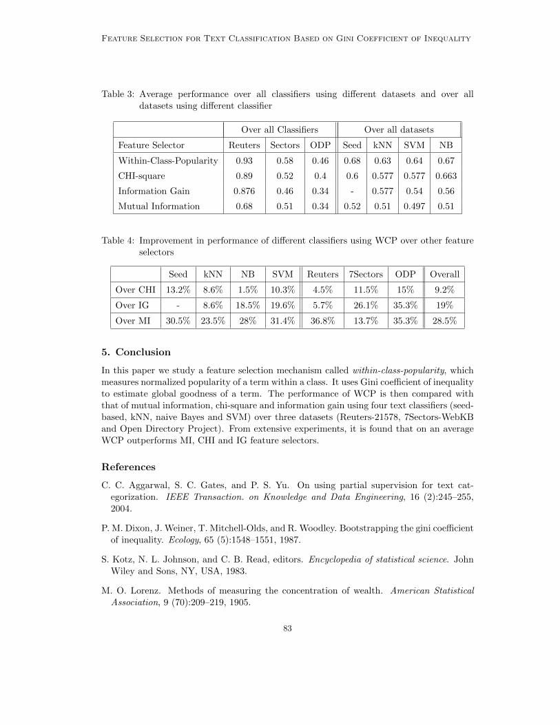
Feature Selection for Text Classification Based on Gini Coefficient of Inequality
Table 3: Average performance over all classifiers using different datasets and over alldatasets using different classifier
Over all Classifiers Over all datasets
Feature Selector Reuters Sectors ODP Seed kNN SVM NB
Within-Class-Popularity 0.93 0.58 0.46 0.68 0.63 0.64 0.67
CHI-square 0.89 0.52 0.4 0.6 0.577 0.577 0.663
Information Gain 0.876 0.46 0.34 - 0.577 0.54 0.56
Mutual Information 0.68 0.51 0.34 0.52 0.51 0.497 0.51
Table 4: Improvement in performance of different classifiers using WCP over other featureselectors
Seed kNN NB SVM Reuters 7Sectors ODP Overall
Over CHI 13.2% 8.6% 1.5% 10.3% 4.5% 11.5% 15% 9.2%
Over IG - 8.6% 18.5% 19.6% 5.7% 26.1% 35.3% 19%
Over MI 30.5% 23.5% 28% 31.4% 36.8% 13.7% 35.3% 28.5%
5. Conclusion
In this paper we study a feature selection mechanism called within-class-popularity, whichmeasures normalized popularity of a term within a class. It uses Gini coefficient of inequalityto estimate global goodness of a term. The performance of WCP is then compared withthat of mutual information, chi-square and information gain using four text classifiers (seed-based, kNN, naive Bayes and SVM) over three datasets (Reuters-21578, 7Sectors-WebKBand Open Directory Project). From extensive experiments, it is found that on an averageWCP outperforms MI, CHI and IG feature selectors.
References
C. C. Aggarwal, S. C. Gates, and P. S. Yu. On using partial supervision for text cat-egorization. IEEE Transaction. on Knowledge and Data Engineering, 16 (2):245–255,2004.
P. M. Dixon, J. Weiner, T. Mitchell-Olds, and R. Woodley. Bootstrapping the gini coefficientof inequality. Ecology, 65 (5):1548–1551, 1987.
S. Kotz, N. L. Johnson, and C. B. Read, editors. Encyclopedia of statistical science. JohnWiley and Sons, NY, USA, 1983.
M. O. Lorenz. Methods of measuring the concentration of wealth. American StatisticalAssociation, 9 (70):209–219, 1905.
83
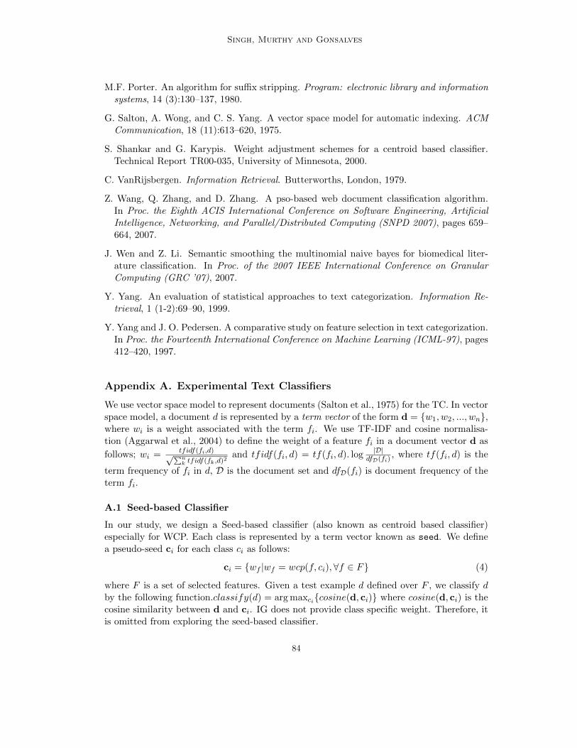
Singh, Murthy and Gonsalves
M.F. Porter. An algorithm for suffix stripping. Program: electronic library and informationsystems, 14 (3):130–137, 1980.
G. Salton, A. Wong, and C. S. Yang. A vector space model for automatic indexing. ACMCommunication, 18 (11):613–620, 1975.
S. Shankar and G. Karypis. Weight adjustment schemes for a centroid based classifier.Technical Report TR00-035, University of Minnesota, 2000.
C. VanRijsbergen. Information Retrieval. Butterworths, London, 1979.
Z. Wang, Q. Zhang, and D. Zhang. A pso-based web document classification algorithm.In Proc. the Eighth ACIS International Conference on Software Engineering, ArtificialIntelligence, Networking, and Parallel/Distributed Computing (SNPD 2007), pages 659–664, 2007.
J. Wen and Z. Li. Semantic smoothing the multinomial naive bayes for biomedical liter-ature classification. In Proc. of the 2007 IEEE International Conference on GranularComputing (GRC ’07), 2007.
Y. Yang. An evaluation of statistical approaches to text categorization. Information Re-trieval, 1 (1-2):69–90, 1999.
Y. Yang and J. O. Pedersen. A comparative study on feature selection in text categorization.In Proc. the Fourteenth International Conference on Machine Learning (ICML-97), pages412–420, 1997.
Appendix A. Experimental Text Classifiers
We use vector space model to represent documents (Salton et al., 1975) for the TC. In vectorspace model, a document d is represented by a term vector of the form d = w1, w2, ..., wn,where wi is a weight associated with the term fi. We use TF-IDF and cosine normalisa-tion (Aggarwal et al., 2004) to define the weight of a feature fi in a document vector d as
follows; wi = tfidf(fi,d)√∑nk tfidf(fk,d)2
and tfidf(fi, d) = tf(fi, d). log |D|dfD(fi)
, where tf(fi, d) is the
term frequency of fi in d, D is the document set and dfD(fi) is document frequency of theterm fi.
A.1 Seed-based Classifier
In our study, we design a Seed-based classifier (also known as centroid based classifier)especially for WCP. Each class is represented by a term vector known as seed. We definea pseudo-seed ci for each class ci as follows:
ci = wf |wf = wcp(f, ci), ∀f ∈ F (4)
where F is a set of selected features. Given a test example d defined over F , we classify dby the following function.classify(d) = arg maxcicosine(d, ci) where cosine(d, ci) is thecosine similarity between d and ci. IG does not provide class specific weight. Therefore, itis omitted from exploring the seed-based classifier.
84

Feature Selection for Text Classification Based on Gini Coefficient of Inequality
A.2 naive Bayes
Assuming naives condition i.e., features are conditionally independent, we defined naiveBayes classifier by
Pr(ck|di) =Pr(ck).
∏j Pr(dij |ck)∏
j Pr(dij)
As denominator is independent of class, effectively, we have estimated Pr(ck|di) as∏
j Pr(dij |ck),where Pr(dij |ck) is defined by Equation 1
A.3 kNN
Cosine similarity is used to estimate distance between test examples and training examples.For each test sample, at most 30 nearest neighbours are considered to count for the winnerclass. In the case of Open Directory Project dataset having very large number of documents,we have randomly selected only 100 test examples from each class and 400 examples fromeach training class and estimated similarity between 1700 test examples and 6800 trainingexamples.
A.4 SVM
We use the SVMTorch software 1 for our reported estimations, which is publicly availablefor download. Again training SVM with large dataset is very expensive. Therefore, likekNN, we have randomly selected only 100 test examples and 400 training examples fromeach class. We run svm tool using linear kernel. From various experiments, we find thatlinear kernel perform better compared to radial and Gaussian kernel.
1. SVMTorch: an SVM software for Classification and Regression, in C++,http://www.idiap.ch/machine-learning.php
85

JMLR: Workshop and Conference Proceedings 10: 86-96 The Fourth Workshop on Feature Selection in Data Mining
Increasing Feature Selection Accuracy for L1 RegularizedLinear Models in Large Datasets
Abhishek Jaiantilal [email protected] of Computer ScienceUniversity of ColoradoBoulder, CO, 80309, USA
Gregory Grudic [email protected]
Flashback Technologies, LLC
Longmont, CO, 80503, USA
Editor: Huan Liu, Hiroshi Motoda, Rudy Setiono, and Zheng Zhao
Abstract
L1 (also referred to as the 1-norm or Lasso) penalty based formulations have been shown tobe effective in problem domains when noisy features are present. However, the L1 penaltydoes not give favorable asymptotic properties with respect to feature selection, and hasbeen shown to be inconsistent as a feature selection estimator; e.g. when noisy features arecorrelated with the relevant features. This can affect the estimation of the correct featureset, in certain domains like robotics, when both the number of examples and the number offeatures are large. The weighted lasso penalty by (Zou, 2006) has been proposed to rectifythis problem of correct estimation of the feature set. This paper proposes a novel methodfor identifying problem specific L1 feature weights by utilizing the results from (Zou, 2006)and (Rocha et al., 2009) and is applicable to regression and classification algorithms. Ourmethod increases the accuracy of L1 penalized algorithms through randomized experimentson subsets of the training data as a fast pre-processing step. We show experimental andtheoretical results supporting the efficacy of the proposed method on two L1 penalizedclassification algorithms.
Keywords: Feature selection, L1 penalized algorithms
1. Introduction
Feature selection using the L1 penalty (also referred as 1-norm or Lasso penalty) has beenshown to perform well when there are spurious features mixed with relevant features andthis property has been extensively discussed in (Efron et al., 2004), (Tibshirani, 1996)and (Zhu et al., 2003). In this paper, we focus on feature selection via the L1 penaltyfor classification, addressing open problems related to feature selection accuracy and largedatasets. This paper is organized as follows, Section-2 presents motivation and background,primarily focusing on the fact that asymptotically L1 penalty based method might includespurious features. Based on the work in (Zou, 2006), we show that random sampling canfind a set of weights that improves accuracy over the unweighted (which is normally used)L1 penalty methods and we detail this in Section-3. In Section-4, we show results on twodifferent classification algorithms and compare the weighted method proposed in (Zou, 2007)with the random sampling method described in our paper. Our method differs from Zou’s
c©2010 Jaiantilal and Grudic.

Increasing Feature Selection Accuracy for L1 Regularized Linear Models
method as it hinges on random sampling to find the weight vector instead of using the L2
penalty. The proposed method is shown to give significant improvement in accuracy over anumber of data sets. Section 5 summarizes the results and concludes with future work.
The contribution of our work is as follows: we show that a fast pre-processing step canbe used to increase the accuracy of L1 regularized models and is a good fit when the numberof examples are large; we connect the theoretical results from (Rocha et al., 2009) showingthe viability of our method on various L1 penalized algorithms and also show empiricalresults supporting our claim.
2. Background Information and Motivation
Consider the following setup in which information about n examples, each with p dimen-sions, is represented in a n x p design matrix denoted by X , with y ∈ Rn representingtarget values/labels, and β ∈ Rp representing a set of model parameters to be estimated.For our paper, we consider classification based linear models with a convex loss function anda penalty term (a regularizer). In (1), we show a regularized formulation that can be usedto generally describe many machine learning algorithms. The metric or loss, L(X, y, β),may represent various loss functions including ‘hinge loss’ for classification based SupportVector Machines (SVMs) and ‘squared error loss’ for regression.
β = argminβL(X, y, β) + λJ(β) (1)
where L(X, y, β) = loss function , J(β) = penalty function and λ ≥ 0
Popular forms of the penalty functions (J(β)) are by using the L2 and L1 norm on β andare termed Ridge and Lasso penalty respectively in literature (refer to (Tibshirani, 1996)).
2.1 Asymptotic properties of L1 penalty
Many papers including (Tibshirani, 1996), (Efron et al., 2004) and (Zhu et al., 2003) discussthe merits of the L1 penalty. The L1 penalty has been shown to be efficient in producingsparse models (models with many of the β’s set to 0) and this feature selecting abilitymakes it robust against noisy features. In addition, the L1 penalty is a convex penalty andwhen used in conjunction with convex loss functions, the resultant formulation has a globalminimum.
As the L1 penalty is used for simultaneous feature selection and correct estimation,a topic of interest is to understand whether sparsity holds when n → ∞, n=number ofexamples. Intuitively, given enough samples, the estimated parameters βn should approachthe true parameters β0.
y = Xβ0 + ε (2)
Assume that the data is generated as shown in (2), with ε being gaussian noise of zeromean and β0 being the true generating model parameters. Also, βjk represents the jth
feature for βk. If A0=j | βj0 6= 0 is the true model and An is the model found for n→∞.
For consistency in feature selection, we need An= j | βjn 6= 0 and limn→∞
P (An = A0)= 1,
that is we find the correct set of features A0 asymptotically. (Zou, 2006) showed that lassoestimator is consistent (in terms of βN → β0) but can be inconsistent as a feature selectingestimator in presence of correlated noisy features.
87
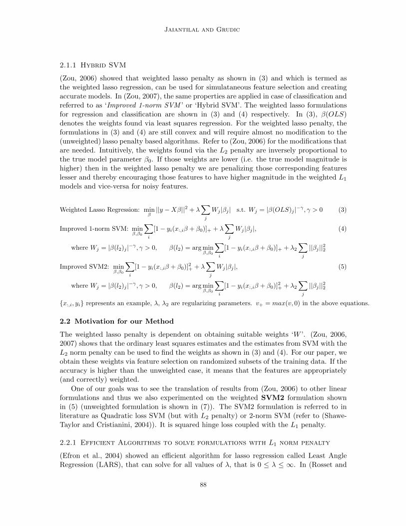
Jaiantilal and Grudic
2.1.1 Hybrid SVM
(Zou, 2006) showed that weighted lasso penalty as shown in (3) and which is termed asthe weighted lasso regression, can be used for simulataneous feature selection and creatingaccurate models. In (Zou, 2007), the same properties are applied in case of classification andreferred to as ‘Improved 1-norm SVM ’ or ‘Hybrid SVM’. The weighted lasso formulationsfor regression and classification are shown in (3) and (4) respectively. In (3), β(OLS)denotes the weights found via least squares regression. For the weighted lasso penalty, theformulations in (3) and (4) are still convex and will require almost no modification to the(unweighted) lasso penalty based algorithms. Refer to (Zou, 2006) for the modifications thatare needed. Intuitively, the weights found via the L2 penalty are inversely proportional tothe true model parameter β0. If those weights are lower (i.e. the true model magnitude ishigher) then in the weighted lasso penalty we are penalizing those corresponding featureslesser and thereby encouraging those features to have higher magnitude in the weighted L1
models and vice-versa for noisy features.
Weighted Lasso Regression: minβ||y −Xβ||2 + λ
∑
j
Wj |βj | s.t. Wj = |β(OLS)j |−γ , γ > 0 (3)
Improved 1-norm SVM: minβ,β0
∑
i
[1− yi(x:,iβ + β0)]+ + λ∑
j
Wj |βj |, (4)
where Wj = |β(l2)j |−γ , γ > 0, β(l2) = arg minβ,β0
∑
i
[1− yi(x:,iβ + β0)]+ + λ2∑
j
||βj ||22
Improved SVM2: minβ,β0
∑
i
[1− yi(x:,iβ + β0)]2+ + λ∑
j
Wj |βj |, (5)
where Wj = |β(l2)j |−γ , γ > 0, β(l2) = arg minβ,β0
∑
i
[1− yi(x:,iβ + β0)]2+ + λ2∑
j
||βj ||22
x:,i, yi represents an example, λ, λ2 are regularizing parameters. v+ = max(v, 0) in the above equations.
2.2 Motivation for our Method
The weighted lasso penalty is dependent on obtaining suitable weights ‘W ’. (Zou, 2006,2007) shows that the ordinary least squares estimates and the estimates from SVM with theL2 norm penalty can be used to find the weights as shown in (3) and (4). For our paper, weobtain these weights via feature selection on randomized subsets of the training data. If theaccuracy is higher than the unweighted case, it means that the features are appropriately(and correctly) weighted.
One of our goals was to see the translation of results from (Zou, 2006) to other linearformulations and thus we also experimented on the weighted SVM2 formulation shownin (5) (unweighted formulation is shown in (7)). The SVM2 formulation is referred to inliterature as Quadratic loss SVM (but with L2 penalty) or 2-norm SVM (refer to (Shawe-Taylor and Cristianini, 2004)). It is squared hinge loss coupled with the L1 penalty.
2.2.1 Efficient Algorithms to solve formulations with L1 norm penalty
(Efron et al., 2004) showed an efficient algorithm for lasso regression called Least AngleRegression (LARS), that can solve for all values of λ, that is 0 ≤ λ ≤ ∞. In (Rosset and
88

Increasing Feature Selection Accuracy for L1 Regularized Linear Models
Zhu, 2007), a generic algorithm, for which LARS is a special case, is documented that canbe used for all double differentiable losses with the L1 penalty. For our experiments, weresort to specific linear SVM based formulations for which entire regularization paths can beconstructed. (6) is the penalized formulation for ‘1-norm SVM’. (Zhu et al., 2003) showeda simple piecewise algorithm to solve for 0 ≤ λ ≤ ∞ in the 1-norm SVM. As the loss andthe penalty function are both singly differentiable, a piecewise path cannot be constructedas efficiently as in LARS but linear programming can be employed to calculate the step size.(7) is an equivalent to (6) and similar to the formulation seen in literature except with theL2 loss function instead of the L1 loss function. (7) is the penalized formulation for squaredhinge loss (or Quadratic loss SVM) with the L1 penalty. As the loss function is doublydifferentiable, via the method described by (Rosset and Zhu, 2007), an efficient piecewisealgorithm that be constructed to solve for 0 ≤ λ ≤ ∞. Our vested interest in using suchpiecewise algorithms, is to help understand whether better (entire) regularization paths arecreated or not for the weighted L1 penalty.
1-norm SVM: minβ,β0
∑
i
[1− yi(x:,iβ + β0)]+ + λ∑
j
|βj |, (6)
Equivalent to (6) : minβ,β0
||β||1 + C∑
i
ξi, s.t. yi(x:,iβ + β0) ≥ 1− ξi, ξi ≥ 0
SVM2: minβ,β0
∑
i
[1− yi(x:,iβ + β0)]2+ + λ∑
j
|βj |, (7)
v+ = max(v, 0) in the above equations.
3. Randomized Sampling (RS) Method to Create Weight Vector
Our randomized sampling method depends on a small random subset of training data. Weassume that the subset of the training data is small, i.e. it is computationally cheap to acton such a set in a reasonable time. Also, such randomized sampling is done multiple times.
3.1 Randomized Sampling (RS) Method
Our randomized sampling algorithm is described below in Algorithm-1: RandomizedSampling Method. The algorithm can be explained as follows: We choose a subset ofm examples out of the presented n examples such that m << n. We train a L1 penaltybased algorithm (e.g. 1-norm SVM (Zhu et al., 2003), SVM2, etc.) so that we can find aset of relevant features. We keep a note of the features that we found in that particularexperiment. After many such randomized experiments, the counts of the number of timesa feature was found in these randomized experiments is summed up and normalized anddenoted by V .
This count vector, denoted by V , is then inverted and used as weights for the weightedversion of the algorithm; i.e. weights used in the weighted formulations are W = 1/V .Intuitively, if a feature is important and is found multiple times via the RS method, thenthe corresponding weight for the feature is less and thus it is penalized lesser, encouraginghigher magnitude for the feature.
89

Jaiantilal and Grudic
Algorithm-1: Randomized Sampling (RS) Method:
Input: n examples each with p features, K randomized experiments, B (Block)number of examples used to train model in each randomized experiment.
Output: Count vector W (1xD vector) representing number of times features wereselected in K randomized experiment.
Divide N examples into K randomized sets each of size B and denote them asNtrni, i = 1 . . .K and let V ←− 0for i = 1 . . .K do
Get Ntrni, construct Ntsti and Nvali set.Train Modeli = L1 Algorithm(Ntrni, Ntsti, Nvali)Si = selected features in Modeli via validation data.V ← V + x, x ∈ RD|xj = 1 if j ∈ Si else xj = 0
end
3.2 Consistency of choosing a set of Features from Randomized Sampling(RS) Experiments
Our method is dependent on finding some set of relevant features and their counts for agiven dataset via the RS method. Our experimental results are restricted to the weightedand unweighted formulation for SVM2 and 1-norm SVM, but our theoretical results areapplicable to all linear models with twice differentiable loss function with the L1 penalty.We next mention results, regarding the asymptotic consistency and normality propertiesin n (number of examples) for L1 penalized algorithms, which can help understand theconsistency of our method.
Lemma 1: This result is from Theorem-5 in (Rocha et al., 2009). If the loss functionL(X, y, β) shown in (1) is bounded, unique and a convex function, with E|L(X, y, β)| <∞and furthermore L(X, y, β) is twice differentiable with a positive hessian H matrix, thenthe following consistency condition defined for the L1 penalty when using the formulationin (1) and true model in (2):
||HAc,A[HA,A −HA,β0H−1β0,β0
Hβ0,A]−1sign(βA)||∞ ≤ 1, where Hx,y =d2L(X, y, β)
dxdy(8)
Where Ac = j ∈ 1...p|βj = 0 , A = j ∈ 1...p|βj 6= 0 and β0 is an intercept.
• if λn is a sequence of non-negative real numbers such that λnn−1 → 0 and λnn
−(1+c)/2 →λ > 0 for some 0 < c < 1/2 as n → ∞ and the condition (8) is satisfied thenP [sign(βn(λn) = sign(β)] ≥ 1 − exp[−nc]. βn is parameter found for number ofexamples=n .
• If the condition in (8) is not satisfied then for any sequence of non-negative numbers λnlimn→∞
P [sign(βn(λn)) = sign(β)] < 1. The probability of choosing incorrect variables
is bounded to exp(−Dnc), where D is a positive constant (shown in the proof ofTheorem 5 of (Rocha et al., 2009)).
If the condition in (8) is fulfilled, it means that the interactions between relevant and noisyfeatures are distinguishable and the L1 penalty can correctly identify the signs in β. If
90

Increasing Feature Selection Accuracy for L1 Regularized Linear Models
the condition in (8) is not fulfilled, then noisy features will be added to the model with aprobability away from 1. Also, note that the above conditions are applicable for 1-normSVM, as shown in (Rocha et al., 2009).
Lemma 2: We use b to specify the size of the subset and assuming b → ∞, then fromLemma-1, when condition of consistency (8) is satisfied then P [sign(βb(λb) = sign(β)] ≥1− exp[−bc] ≈ 1, where βb and λb represent the parameters for the subset of size b. For ksuch subsets V , as depicted in the algorithm in Section 3.1, is bounded to k(1−exp[−bc]) ≈k, b → ∞. When the condition in (8) is not satisfied then the probability of choosingnoisy variables in a subset is upperbounded to exp(−Dbc) and for k subsets, sum(Vj) ≤k · exp(−Dbc) and Vj ≈ 0, b → ∞, (where Vj are indices of noisy variables). Thus, thenoisy variables have a probability of having a low count in V and a large weight in W , thuspenalizing the noisy features heavily .
Table 1: Mean ± Std. Deviation of Error Rates in % on Models 1 & 4 by SVM2q p 2-norm SVM2 1-norm SVM2 Hybrid (Zou) RS(20%) RS(30%) RS(40%)2 14 9.64±2.30 7.92±1.89 7.88±2.09 7.69±1.71 7.67±1.66 7.68±1.694 27 10.90±2.41 8.01±1.84 7.88±2.09 7.73±1.59 7.73±1.59 7.71±1.606 44 12.17±2.64 7.93±1.79 7.79±1.69 7.64±1.60 7.64±1.59 7.64±1.528 65 13.45±2.96 8.13±2.10 7.87±1.84 7.82±1.85 7.83±1.85 7.81±1.8312 119 16.91±3.24 8.11±1.95 8.05±1.94 7.78±1.71 7.78±1.70 7.76±1.6616 189 17.93±3.32 7.87±1.78 8.29±2.41 7.66±1.57 7.66±1.63 7.66±1.6320 275 19.31±3.32 8.06±2.14 8.04±2.01 7.69±1.81 7.74±1.89 7.77±1.87
Random Sampling is Subsampling: To better quantify our random sampling method,we explain it in terms of subsampling (refer to (Politos et al., 1999)). Subsampling is amethod of sampling m examples from n total examples with m < n, unlike bootstrap thatsamples n times with replacement from n samples. Let estimator θ be a general function ofi.i.d data generated from some probability distribution P . In our case of feature selection,this estimator is the feature set. We are interested in finding an estimator and it’s confidenceregion based on the probability P of the data and we define it as θ(P ). When P is largethen we can construct an empirical estimator θn of θ(P ) such that θn = θ(Pn), where Pnis the empirical distribution; that is estimate the true feature set empirically. We define aroot of form τn(θ− θ), where τn is some sequence (like
√n or n) increasing with n (number
of examples), and we are looking at the difference between the empirical estimator θn andthe true estimator θ. We define Jn(P ) to be the sampling distribution of τn(θ−θ(F )) basedon a sample size of n from P and define the CDF as
Jn(x, P ) = ProbabilityP τn(θn − θ) ≤ x, x ∈ R (9)
Lemma 3: From (Politos et al., 1999), for data generated via i.i.d., there is a limiting lawJ(P ) such that Jn(P ) converges weakly (in probability) to J(P ) and τb(θn − θ) → 0 asn→∞ with the conditions that τb/τn → 0, b→∞ and b/n→ 0, where b is the number ofexamples in the subsample experiment and n is the total number of available examples.
Lemma 3, has remarkably weak conditions for subsampling and it requires that the roothas some limiting distribution and the sample size b is not too large (but still going toinfinity) compared to n . In our case, the subsets are of size b → ∞, b << n and for therate of estimation at τn ∝ nc, τb ∝ bc, 0 < c ≤ 1, then τb/τn → 0. For the RS method,we create weight vector whose index for a feature is non-zero if that feature was found in
91

Jaiantilal and Grudic
Table 2: Mean ± Std. Deviation of Error Rates in % on on Models 1 & 4 by 1-norm SVM
q p 2-norm SVM 1-norm SVM Hybrid (Zou) RS(20%) RS(30%) RS(40%)2 14 8.74±1.30 7.64±0.09 7.64±1.02 7.63±1.02 7.64±1.01 7.53±0.094 27 9.76±1.75 7.85±1.14 7.95±1.34 7.83±1.28 7.79±1.24 7.69±1.196 44 10.57±1.95 7.85±1.01 7.92±1.12 7.79±1.12 7.77±1.18 7.69±1.238 65 11.47±2.31 7.81±0.99 7.99±1.36 7.75±1.13 7.74±1.15 7.63±1.0912 119 13.27±2.48 7.91±0.98 8.04±1.35 7.77±1.16 7.82±1.21 7.63±1.0016 189 15.58±2.94 7.94±1.15 7.87±1.21 7.74±1.31 7.75±1.23 7.64±1.1420 275 17.14±2.96 7.90±1.00 7.85±1.11 7.77±1.20 7.80±1.27 7.69±1.19
a particular experiment. θn is the sample mean of n such RS experiments weights, havingmean converging to θ(P ) (due to Lemma-2). Thus estimating the true feature set on basisof random sampling of subsets of data is weakly convergent. (Zou, 2006) used a root-n-consistent estimator’s weight (from the L2 penalty) but mentions that the conditions can befurther weakened and if there is an an such that an →∞ and an(θ−θ) = O(1) then such anestimator can also be used. By Lemma-3, our RS estimator is one such consistent estimatorand thus can be used as a valid estimator for usage with the weighted lasso penalty.
4. Algorithms and Experiments
In this paper, we limit ourselves to an empirical study of data block sizes for the RSestimator. We replicate the experiments from ‘An Improved 1-norm SVM for SimultaneousClassification and Variable Selection’ by (Zou, 2007) and report on 1-norm SVM and SVM2.
Method for choosing Weights (for Hybrid and RS) and Validation data (forRS): For the Hybrid SVM, in order to find the optimal weights via L2 penalty, we usethe method described by (Zou, 2007). We first find the best SVM (or SVM2) algorithmmodel weights (β(l2)) with the L2 penalty via a parameteric search over costs C=0.1, 0.5,1, 2, 5, 10. We then create entire piecewise paths for various weight values |β(l2)|−γ , γ =1, 2, 4; choose the best performing model on validation data and then report on the testdataset. Description on how we chose training set for the RS method is given in individualexperiments. Our RS experiments need validation data to help choose the relevant featuresfor each of the RS training set. We do the following: if n is the size of the training setand we choose m of those examples for the current RS training set, we just use the leftout n−m examples (as validation) for choosing the best features from the piecewise pathsgenerated by the L1 algorithm on the m examples. In case, if a held out validation set waspresent, we use that instead.
4.1 Synthetic Datasets
We simulate two synthetic datasets, one akin to “orange data” described in (Zhu et al.,2003) and another a bernoulli distribution based dataset. The following notation is usedfor some of the tables: We use “C” and “IC” to denote the mean number of correctlyand incorrectly selected features, respectively. Also, we resort to reporting to mean andstd. deviation as the median of the incorrectly selected features was 0 for many experi-ments. “PPS” stands for the probability of perfect selection, i.e the probability ofonly choosing the correct feature set.
92
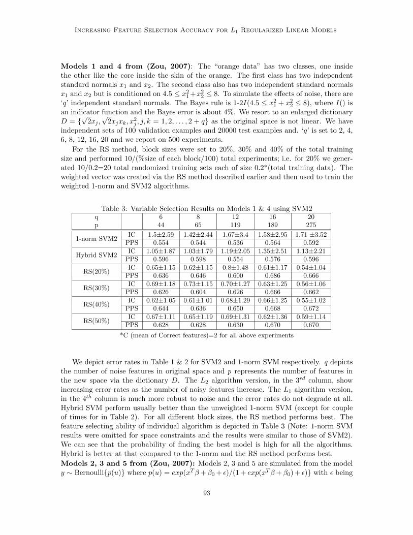
Increasing Feature Selection Accuracy for L1 Regularized Linear Models
Models 1 and 4 from (Zou, 2007): The “orange data” has two classes, one insidethe other like the core inside the skin of the orange. The first class has two independentstandard normals x1 and x2. The second class also has two independent standard normalsx1 and x2 but is conditioned on 4.5 ≤ x21+x22 ≤ 8. To simulate the effects of noise, there are‘q’ independent standard normals. The Bayes rule is 1-2I(4.5 ≤ x21 + x22 ≤ 8), where I() isan indicator function and the Bayes error is about 4%. We resort to an enlarged dictionaryD =
√2xj ,√
2xjxk, x2j , j, k = 1, 2, . . . , 2 + q as the original space is not linear. We have
independent sets of 100 validation examples and 20000 test examples and. ‘q’ is set to 2, 4,6, 8, 12, 16, 20 and we report on 500 experiments.
For the RS method, block sizes were set to 20%, 30% and 40% of the total trainingsize and performed 10/(%size of each block/100) total experiments; i.e. for 20% we gener-ated 10/0.2=20 total randomized training sets each of size 0.2*(total training data). Theweighted vector was created via the RS method described earlier and then used to train theweighted 1-norm and SVM2 algorithms.
Table 3: Variable Selection Results on Models 1 & 4 using SVM2q 6 8 12 16 20p 44 65 119 189 275
1-norm SVM2IC 1.5±2.59 1.42±2.44 1.67±3.4 1.58±2.95 1.71 ±3.52
PPS 0.554 0.544 0.536 0.564 0.592
Hybrid SVM2IC 1.05±1.87 1.03±1.79 1.19±2.05 1.35±2.51 1.13±2.21
PPS 0.596 0.598 0.554 0.576 0.596
RS(20%)IC 0.65±1.15 0.62±1.15 0.8±1.48 0.61±1.17 0.54±1.04
PPS 0.636 0.646 0.600 0.686 0.666
RS(30%)IC 0.69±1.18 0.73±1.15 0.70±1.27 0.63±1.25 0.56±1.06
PPS 0.626 0.604 0.626 0.666 0.662
RS(40%)IC 0.62±1.05 0.61±1.01 0.68±1.29 0.66±1.25 0.55±1.02
PPS 0.644 0.636 0.650 0.668 0.672
RS(50%)IC 0.67±1.11 0.65±1.19 0.69±1.31 0.62±1.36 0.59±1.14
PPS 0.628 0.628 0.630 0.670 0.670
*C (mean of Correct features)=2 for all above experiments
We depict error rates in Table 1 & 2 for SVM2 and 1-norm SVM respectively. q depictsthe number of noise features in original space and p represents the number of features inthe new space via the dictionary D. The L2 algorithm version, in the 3rd column, showincreasing error rates as the number of noisy features increase. The L1 algorithm version,in the 4th column is much more robust to noise and the error rates do not degrade at all.Hybrid SVM perform usually better than the unweighted 1-norm SVM (except for coupleof times for in Table 2). For all different block sizes, the RS method performs best. Thefeature selecting ability of individual algorithm is depicted in Table 3 (Note: 1-norm SVMresults were omitted for space constraints and the results were similar to those of SVM2).We can see that the probability of finding the best model is high for all the algorithms.Hybrid is better at that compared to the 1-norm and the RS method performs best.
Models 2, 3 and 5 from (Zou, 2007): Models 2, 3 and 5 are simulated from the modely ∼ Bernoullip(u) where p(u) = exp(xTβ+ β0 + ε)/(1 + exp(xTβ+ β0) + ε) with ε being
93
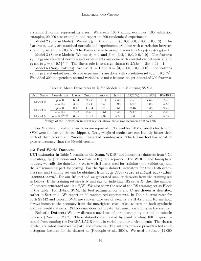
Jaiantilal and Grudic
a standard normal representing error. We create 100 training examples, 100 validationexamples, 20,000 test examples and report on 500 randomized experiments.
Model 2 (Sparse Model): We set β0 = 0 and β = 3, 0, 0, 0, 0, 3, 0, 0, 0, 0, 0, 3. Thefeatures x1, ...x12 are standard normals and experiments are done with correlation betweenxi and xj set to ρ = 0, 0.5. The Bayes rule is to assign classes to 2I(x1 + x6 + x12)− 1.
Model 3 (Sparse Model): We use β0 = 1 and β = 3, 2, 0, 0, 0, 0, 0, 0, 0. The featuresx1, ...x12 are standard normals and experiments are done with correlation between xi andxj set to ρ = 0, 0.5|i−j|. The Bayes rule is to assign classes to 2I(3x1 + 2x2 + 1)− 1.
Model 5 (Noisy features): We use β0 = 1 and β = 3, 2, 0, 0, 0, 0, 0, 0, 0. The features
x1, ...x12 are standard normals and experiments are done with correlation set to ρ = 0.5|i−j|.We added 300 independent normal variables as noise features to get a total of 309 features.
Table 4: Mean Error rates in % for Models 2, 3 & 5 using SVM2
Exp. Name Correlation Bayes 2-norm 1-norm Hybrid RS(20%) RS(30%) RS(40%)
Model 2ρ = 0 6.04 9.77 8.14 7.46 7.51 7.53 7.55ρ = 0.5 4.35 7.74 6.43 5.96 5.97 5.86 5.86
Model 3ρ = 0 8.48 11.04 9.79 9.54 9.46 9.46 9.45ρ = 0.5 7.03 8.49 9.51 8.45 8.17 8.17 8.20
Model 5 ρ = 0.5|i−j| 6.88 31.31 9.32 8.5 8.6 8.56 8.22
*range of std. deviation in accuracy for above table was between 1.02 to 1.96.
For Models 2, 3 and 5: error rates are reported in Table-4 for SVM2 (results for 1-normSVM were similar and hence skipped). Note, weighted models are consistently better thanboth of their 1-norm and 2-norm unweighted counterparts. The RS method has equal orgreater accuracy than the Hybrid version.
4.2 Real World Datasets
UCI datasets: In Table 5, results on the Spam, WDBC and Ionosphere datasets from UCIrepository, by (Asuncion and Newman, 2007), are reported. For WDBC and Ionospheredataset, we split the data into 3 parts with 2 parts used for training (and validation) andthe 3rd remaining part for testing. For the Spam dataset, indicators for test (1536 exam-ples) set and training set can be obtained from http://www-stat.stanford.edu/~tibs/
ElemStatLearn/. For our RS method we generated smaller datasets from the training setas follows: If the training set size is N and size for individual RS set is K, then the numberof datasets generated are 10 ∗N/K. We also show the size of the RS training set as Blockin the table. For Hybrid SVM, the best parameter for γ and C are chosen as describedearlier in Section 4. We report on 50 randomized experiments. In Table 5, error rates forboth SVM2 and 1-norm SVM are shown. The use of weights via Hybrid and RS method,always increases the accuracy from the unweighted case. Also, as seen on both syntheticand real world datasets, RS blocksize does not create that much variability in the results.
Robotic Dataset: We now discuss a novel use of our subsampling method on roboticdatasets (Procopio, 2007). These datasets are created by hand labeling 100 images ob-tained from running the DARPA LAGR robot in varied outdoor environments. The classeslabeled are robot traverseable path and obstacles. The authors provide pre-extracted colorhistogram features for the dataset at (Procopio et al., 2009). We used a subset (12,000
94

Increasing Feature Selection Accuracy for L1 Regularized Linear Models
Table 5: Mean ± Std. Deviation of Error Rates on Real world Datasets
Dataset AlgorithmWithout Randomized Hybrid
2-norm SVMWeighting Sampling SVM
(Name/Block) Weighting
WDBC
1-norm (100)3.66 ± 1.17
2.79 ± 0.93 2.89 ± 0.79
4.05 ± 1.361-norm (150) 2.79 ± 0.90 3.16 ± 1.22SVM2 (100)
3.55 ± 1.812.78 ± 1.03 2.73 ± 1.01
SVM2 (150) 2.90 ± 1.15 2.91 ± 1.13
SPAM
1-norm (200)9.09 ± 0.878
8.18 ± 0.49 8.31 ± 0.61
7.06 ± 0.041-norm (1000) 7.53 ± 0.17 8.19 ± 0.73SVM2 (200)
8.45 ± 3.437.38 ± 0.52 7.39 ± 0.30
SVM2 (1000) 7.70 ± 2.73 7.48 ± 0.52
Ionosphere
1-norm (50)12.38 ± 2.04
11.52 ± 1.39 11.84 ± 1.38
13.03 ± 2.86
1-norm (75) 11.25 ± 1.98 11.56 ± 1.731-norm (100) 11.29 ± 1.65 11.72 ± 1.23SVM2 (50)
12.69 ± 2.8211.43 ± 2.52 11.21 ± 2.66
SVM2 (75) 11.61 ± 2.50 11.22 ± 2.58SVM2 (100) 11.37 ± 2.67 11.26 ± 2.68
Table 6: Avg. Error rate on Robotic Datasets from (Procopio, 2007)DS1A DS2A DS3A
Unweighted SVM2 8.92 4.36 1.24Weighted SVM2 6.41 4.13 1.15
examples) of the available data for each of the 100 frames. Each example is 15 dimen-sional. We set our experimentation as follows: for each frame Fi, i is the index of theframe, we divide the obtained examples (12K examples) into 8 folds (9.6K examples) fortraining, 1 fold (1.2K examples) for validation and 1 fold (1.2K examples) for testing. Wetrain/validate/test on the unweighted SVM2 algorithm. For the weighted experiment, wetrain via our RS method, by dividing the training into 10 subsets (each 960 examples) andfinding the weight vector. This weight vector is then used to create the weighted SVM2models and we report on the test set. Now, instead of discarding weights when a new framearrives, we use the weights found in frame Fi again in Fi+1, i.e. if weights in frame Fi arenoted as Wi then:
Wi+1 ← Wi + weight results of RS for frame Fi+1This is one experimental environment, where creating L2 models for the entire data is not
feasible and the RS estimator is a potential approach. Also, propagating feature importancebetween frames is an advantage for the RS estimator. In Table-6, we show overall results for100 frames for 3 datasets done 10 times. We propagate the weights for the weighted SVM2between frames. As shown, there is a drop in error rates (between 5-28%) for the weightedSVM2 compared to the unweighted SVM2. The overhead of computing the weights via RSwas < 10% that of computing a model for the entire training set.
5. Conclusions and Future work
A Random Sampling framework is presented and is empirically shown to give effectivefeature weights to the lasso penalty, resulting in both increased model accuracy and featureselection accuracy. The proposed framework is at least as effective (and at times more
95

Jaiantilal and Grudic
effective than) the Hybrid SVM, with the added benefit of significantly lower computationalcost. In addition, unlike the Hybrid SVM which must see all the data at once, RandomSampling is shown to be effective in an on-line setting where predictions must be madebased on only partially available data (as in data taken from the robotics domain). In thispaper the framework is demonstrated on two types of linear classification algorithms, andtheoretical support is presented showing its applicability, in general, to sparse algorithms.
References
A. Asuncion and D.J. Newman. UCI machine learning repository, 2007. URL http://www.
ics.uci.edu/~mlearn/MLRepository.html.
Bradley Efron, Trevor Hastie, Iain Johnstone, and Robert Tibshirani. Least angle regression.Annals of Statistics, 32:407–499, 2004.
Dimitris N. Politos, Joseph P. Romano, and Michael Wolf. Subsampling. Springer, 1999.
Michael J. Procopio. Hand-labeled DARPA LAGR datasets. Available at http://ml.cs.
colorado.edu/~procopio/labeledlagrdata/, 2007.
Michael J. Procopio, Jane Mulligan, and Greg Grudic. Learning terrain segmentation withclassifier ensembles for autonomous robot navigation in unstructured environments. Jour-nal of Field Robotics, 26(2):145–175, 2009. doi: http://dx.doi.org/10.1002/rob.20279.
Guilherme V. Rocha, Xing Wang, and Bin Yu. Asymptotic distribution and sparsistencyfor l1-penalized parametric m-estimators with applications to linear svm and logisticregression, 2009. URL http://www.citebase.org/abstract?id=oai:arXiv.org:0908.
1940.
Saharon Rosset and Ji Zhu. Piecewise linear regularized solution paths. Annals of Statistics,(35), 2007.
John Shawe-Taylor and Nello Cristianini. Kernel methods for pattern analysis. CambridgeUniversity Press, 2004.
Robert Tibshirani. Regression shrinkage and selection via the lasso. Journal of the RoyalStatistical Society, Series B, 58:267–288, 1996.
Ji Zhu, Saharon Rosset, Trevor Hastie, and Rob Tibshirani. 1-norm support vector ma-chines. In Neural Information Processing Systems, page 16. MIT Press, 2003.
Hui Zou. The adaptive lasso and its oracle properties. Journal of the American StatisticalAssociation, 101:1418–1429(12), December 2006.
Hui Zou. An improved 1-norm svm for simultaneous classification and variable selection.AISTATS, 2:675–681, 2007.
96
JMLR: Workshop and Conference Proceedings 10: 97-106 The Fourth Workshop on Feature Selection in Data Mining
Learning Dissimilarities for Categorical Symbols
Jierui Xie [email protected]
Boleslaw Szymanski [email protected]
Mohammed J. Zaki [email protected]
Department of Computer Science
Rensselaer Polytechnic Institute
Troy, NY 12180, USA
Editor: Huan Liu, Hiroshi Motoda, Rudy Setiono, and Zheng Zhao
Abstract
In this paper we learn a dissimilarity measure for categorical data, for effective classificationof the data points. Each categorical feature (with values taken from a finite set of sym-bols) is mapped onto a continuous feature whose values are real numbers. Guided by theclassification error based on a nearest neighbor based technique, we repeatedly update theassignment of categorical symbols to real numbers to minimize this error. Intuitively, thealgorithm pushes together points with the same class label, while enlarging the distances topoints labeled differently. Our experiments show that 1) the learned dissimilarities improveclassification accuracy by using the affinities of categorical symbols; 2) they outperform dis-similarities produced by previous data-driven methods; 3) our enhanced nearest neighborclassifier (called LD) based on the new space is competitive compared with classifiers suchas decision trees, RBF neural networks, Naıve Bayes and support vector machines, on arange of categorical datasets.
Keywords: Dissimilarity, Categorical Data, Learning Algorithm, Classification, FeatureSelection
1. Introduction
The notion of distance plays an important role in many data mining tasks, such as classi-fication, clustering, and outlier detection. However, the notion of distance for categoricaldata is rarely defined precisely, if at all. By categorical or symbolic data, we refer to valuesthat are nominal (e.g. colors) or ordinal (e.g. rating, typically imposed subjectively by ahuman). In many cases, the dissimilarities between symbols are fuzzy and often arbitrary.An example could be the rating of a movie, chosen from the list “very bad, bad, fair, good,very good”. It is hard to determine how much one symbol differs from another. In thispaper, we introduce a new method to derive dissimilarities between categorical symbols insuch a way that the power of distance-based data mining methods can be applied.
The notations used throughout the paper are as follows. There is a dataset X =x1,x2, . . . ,xt of t data points, where each point xi is a tuple of m attributes values,xi = (x1
i , . . . , xmi ). Each of the m attributes Ai is categorical, i.e., the attribute values for
Ai are drawn from a set of ni discrete values given as ai1, ai2, . . . , aini, which also consti-
tute the domain of Ai. We assume that all symbols across all attributes are unique. Forsimplicity, we use the notation Ai to refer to the i-th attribute, as well as the domain of
c©2010 Xie, Szymanski and Zaki.

Xie, Szymanski and Zaki
that attribute. Each aij is also called a symbol. Each data point xi (in the training set) alsohas associated with the “true” class label, given as L(xi). In this paper we only considerthe case where there are two classes, i.e., L(xi) ∈ 1, 2, where 1 and 2 are the two classlabels.
The similarity between symbols aik and ail of an attribute Ai is denoted as S(aik, ail),
whereas the dissimilarity or distance between two symbols is denoted as D(aik, ail). Typically
S(aik, ail) : Ai×Ai → (0, 1), in which case D(aik, a
il) = 1−S(aik, a
il). In other cases S(aik, a
il) :
Ai×Ai → R+, in which case D(aik, ail) = 1
S(aik,ail)
. The distance between two data points xi
and xj is defined in terms of the distance between symbols, as follows:
D(xi,xj) =
√√√√m∑
k=1
D(xki , xkj )2 (1)
Given a point xi, the error of a classifier on that point is defined as:
exi =(L(xi)−O(xi))
2
2(2)
where O(xi) is the output class of the classifier on point xi. Since O(xi) ∈ 1, 2, exi ∈0, 1
2. The total error rate of the classifier on a set of t points is simply E =∑t
i=1 exi .In this paper, our goal is to learn a mapping function from each categorical attribute Ai
onto the real number interval, given by the function r : Ai → R, with the aim of minimizingthe total error rate E. Once r has been learned, each categorical data point xi can betreated as a m-dimensional point or vector in Rm, given as r(xi) = (r(xi,1), . . . , r(xi,m))T .This enables one to apply any of the distance-based classification methods directly on thetransformed dataset r(X) = r(xi)ti=1.
(a) (b) (c)
Figure 1: (a) Mapping symbols to real values. Dataset consists of three points: x1 = (A, a),x2 = (B, b) and x3 = (C, c). The mapping function r is given as: r(A) = 0.1,r(B) = 0.2, r(C) = 0.6, r(a) = 0.5, r(b) = 0.4 and r(c) = 0.1. (b) Randommapping. (c) Linearly separable mapping.
As an example, consider Figure 1 (a), which shows three points over two categoricalattributes “color” (with symbols A, B and C) and “shape” (with symbols a, b and c). In
98
Learning Dissimilarities for Categorical Symbols
the new continuous space, a value assignment to a symbol naturally defines a hyperplanethat contains all the points in the dataset having that particular symbol. In this example,each point is defined by exactly two straight lines. Figure 1 (b) shows an extended examplewith 8 points, with a random initial mapping, which does not discriminate too well betweenthe two classes. Our goal is to improve the initial mapping into a classification-awaremapping like that in Figure 1 (c), which achieves a low classification error rate (on thetraining set, and hopefully on the test set too).
2. Related Work
The most widely used measure on categorical data is simple matching (or overlap), which isdefined as S(ai, aj) = 1 if ai = aj and S(ai, aj) = 0, otherwise. This measure simply checksthat two symbols are the same, which forms the basis for various distance functions, suchas Hamming and Jaccard distance (Liang, 2004).
The simple matching ignores information from the dataset and the desired classification.Therefore, many more data-driven measures have been developed to capture preferences formatching or mismatching based on symbols’ statistics. Here, we divide related methodsinto two categories: unsupervised and supervised methods. The unsupervised methods aretypically based on frequency or entropy. Let f(ai) be the frequency of symbol ai of attributeA in the dataset, then p(ai) = f(ai)/t.
Let ai and aj be two symbols in the domain of attribute A. Lin (1998) defines S(ai, aj) =2 log p(ai) if ai = aj , and 2 log(p(ai)+p(aj)), otherwise, which gives more weight to matcheson frequent values and lower weight to mismatches on infrequent values. Burnaby (1970)defines S(ai, aj) = 1 if ai = aj . However, if ai 6= aj , then
S(ai, aj) =
∑ak∈A 2 log(1− p(ak))
log(
p(ai)p(aj)(1−p(ai))(1−p(aj))
)+∑
ak∈A 2 log(1− p(ak))
Smirnov (1968) not only considers the frequency, but also takes the distribution of the otherattributes values into account, defining
S(ai, aj) = 2 +t− f(ai)
f(ai)+
∑
ak∈A\ai
f(ak)
t− f(ak)
if ai = aj , and
S(ai, aj) =∑
ak∈A\ai,aj
f(ak)
n− f(ak)
otherwise. Goodall (1966) proposed another statistical approach, in which less frequentattribute values make greater contribution to the overall similarity than frequent attributevalues. A modified version called Goodall1 is proposed in (Boriah et al., 2008), defining
S(ai, aj) = 1−∑
ak∈A,p(ak)<p(ai)
p2(ak)
if ai = aj , and 0 otherwise. Gambaryan (1964) proposed a measure related to informationentropy, which gives more weight to matches where the number of matches is between
99
Xie, Szymanski and Zaki
frequent and rare. If ai = aj , the similarity is given as
S(ai, aj) = −[p(ai) log2 p(ai) + (1− p(ai)) log2(1− p(ai))]
and 0 otherwise. Eskin et al. (2002) consider the number of symbols of each attribute. Inits modified version (Boriah et al., 2008), this measure gives more weight to mismatchesthat occur on an attribute with more symbols using the weight n2/(n2 + 2), where n is thenumber of symbols of attribute A. Occurrence Frequency (OF) (Jones, 1988) gives lowersimilarity to mismatches on less frequent symbols and higher similarity on mismatches onmore frequent symbols. Conversely, Inverse Occurrence Frequency (IOF) assigns highersimilarity to mismatches on less frequent symbols. That is, if ai 6= aj , then
S(ai, aj) =1
1 + log( nf(ai)
) log( nf(aj))
for OF, and
S(ai, aj) =1
1 + log(f(ai)) log(f(aj))
for IOF. When ai = aj , both define S(ai, aj) = 1. More discussion on these kinds ofmeasures is given by Boriah et al. (2008).
The supervised methods take advantage of the class information. An example is ValueDifference Metric (VDM) proposed in (Stanfill and Waltz, 1986). The main idea is thatsymbols are similar if they occur with a similar relative frequency for all the classes. Thedissimilarity between ai and aj is defined as a sum over n classes:
D(ai, aj) =n∑
c=1
∣∣∣∣Cai,c
Cai
− Caj ,c
Caj
∣∣∣∣h
where Cai,c is the number of times symbol ai occurs in class c. Cai is the total number oftimes ai occurs in the whole dataset. Constant h is usually set to 1. Cheng et al. (2004)proposed an approach based on Hadamard product and RBF classifier. They attempt toevaluate all the pair-wise distances between symbols, and they optimize the error functionusing gradient descent method. In our algorithm the number of values to be estimatedis equal to the number of symbols across all attributes, i.e. linear in the symbol set size,which may enable faster and more robust learning. However, we were unable to comparethe methods directly since we did not have access to the code from Cheng et al. (2004).Furthermore, in our approach, after learning, all pair-wise distances can be easily derivedif needed.
3. Learning Algorithm
Our learning algorithm is based on the gradient descent method. Starting from an initialassignment of real values to the symbols, guided by the error rate based on a nearest neighborclassifier, our method iteratively updates the assignments. Intuitively, in each iteration, themethod moves the symbols (hence the lines or, more generally, the hyperplanes, as seenin Figure 1) to new locations according to the net force imposed on them. Let x be the
100
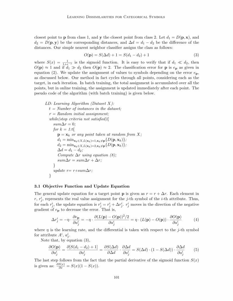
Learning Dissimilarities for Categorical Symbols
closest point to p from class 1, and y the closest point from class 2. Let d1 = D(p,x), andd2 = D(p,y) be the corresponding distances, and ∆d = d1 − d2 be the difference of thedistances. Our simple nearest neighbor classifier assigns the class as follows:
O(p) = S(∆d) + 1 = S(d1 − d2) + 1 (3)
where S(x) = 11+e−x is the sigmoid function. It is easy to verify that if d1 d2, then
O(p) ≈ 1 and if d1 d2 then O(p) ≈ 2. The classification error for p is ep as given inequation (2). We update the assignment of values to symbols depending on the error ep,as discussed below. Our method in fact cycles through all points, considering each as thetarget, in each iteration. In batch training, the total assignment is accumulated over all thepoints, but in online training, the assignment is updated immediately after each point. Thepseudo code of the algorithm (with batch training) is given below.
LD: Learning Algorithm (Dataset X):t = Number of instances in the dataset;r = Random initial asssignment;while(stop criteria not satisfied)sum∆r = 0;for k = 1:t
p = xk or any point taken at random from X;d1 = minxk∈X,L(xk)=1,xk 6=pD(p,xk);d2 = minxk∈X,L(xk)=2,xk 6=pD(p,xk);∆d = d1 − d2;Compute ∆r using equation (8);sum∆r = sum∆r + ∆r;update r= r+sum∆r;
3.1 Objective Function and Update Equation
The general update equation for a target point p is given as r = r + ∆r. Each element inr, rij , represents the real value assignment for the j-th symbol of the i-th attribute. Thus,
for each rij , the update equation is rij = rij + ∆rij . rij moves in the direction of the negative
gradient of ep to decrease the error. That is,
∆rij = −η · ∂ep∂aij
= −η · ∂(L(p)−O(p))2/2
∂aij= η · (L(p)−O(p)) · ∂O(p)
∂aij(4)
where η is the learning rate, and the differential is taken with respect to the j-th symbolfor attribute Ai, aij .
Note that, by equation (3),
∂O(p)
∂aij=∂[S(d1 − d2) + 1]
∂aij=∂S(∆d)
∂∆d· ∂∆d
∂aij= S(∆d) · (1− S(∆d)) · ∂∆d
∂aij(5)
The last step follows from the fact that the partial derivative of the sigmoid function S(x)
is given as: ∂S(x)∂x = S(x)(1− S(x)).
101
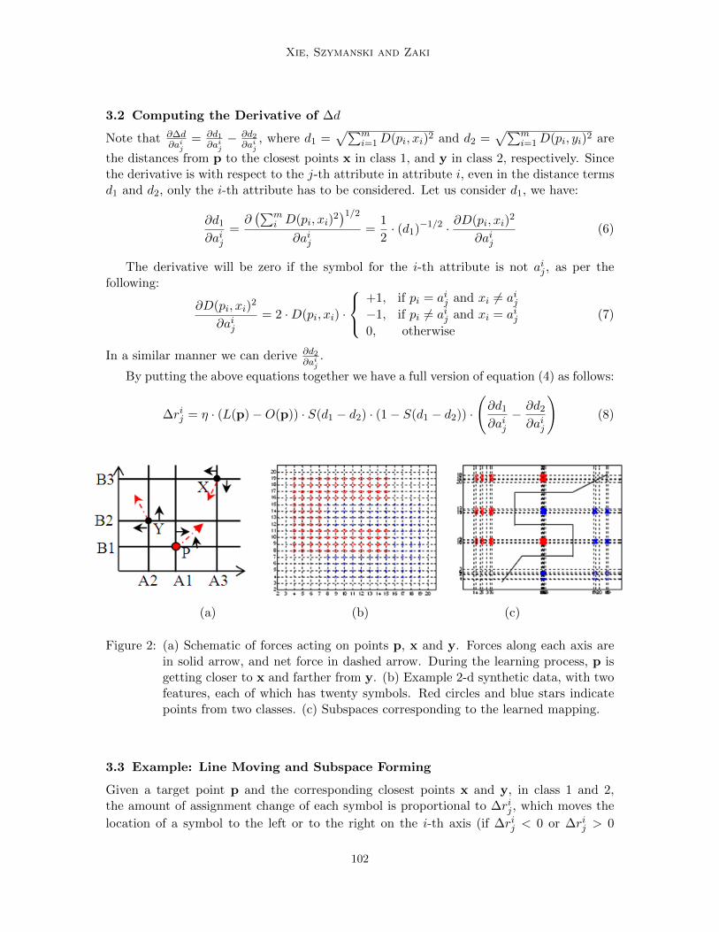
Xie, Szymanski and Zaki
3.2 Computing the Derivative of ∆d
Note that ∂∆d∂aij
= ∂d1∂aij− ∂d2
∂aij, where d1 =
√∑mi=1D(pi, xi)2 and d2 =
√∑mi=1D(pi, yi)2 are
the distances from p to the closest points x in class 1, and y in class 2, respectively. Sincethe derivative is with respect to the j-th attribute in attribute i, even in the distance termsd1 and d2, only the i-th attribute has to be considered. Let us consider d1, we have:
∂d1
∂aij=∂(∑m
i D(pi, xi)2)1/2
∂aij=
1
2· (d1)−1/2 · ∂D(pi, xi)
2
∂aij(6)
The derivative will be zero if the symbol for the i-th attribute is not aij , as per thefollowing:
∂D(pi, xi)2
∂aij= 2 ·D(pi, xi) ·
+1, if pi = aij and xi 6= aij−1, if pi 6= aij and xi = aij0, otherwise
(7)
In a similar manner we can derive ∂d2∂aij
.
By putting the above equations together we have a full version of equation (4) as follows:
∆rij = η · (L(p)−O(p)) · S(d1 − d2) · (1− S(d1 − d2)) ·(∂d1
∂aij− ∂d2
∂aij
)(8)
(a) (b) (c)
Figure 2: (a) Schematic of forces acting on points p, x and y. Forces along each axis arein solid arrow, and net force in dashed arrow. During the learning process, p isgetting closer to x and farther from y. (b) Example 2-d synthetic data, with twofeatures, each of which has twenty symbols. Red circles and blue stars indicatepoints from two classes. (c) Subspaces corresponding to the learned mapping.
3.3 Example: Line Moving and Subspace Forming
Given a target point p and the corresponding closest points x and y, in class 1 and 2,the amount of assignment change of each symbol is proportional to ∆rij , which moves the
location of a symbol to the left or to the right on the i-th axis (if ∆rij < 0 or ∆rij > 0
102
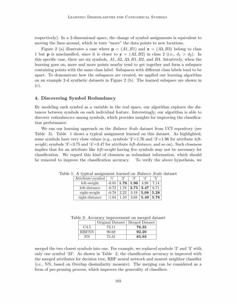
Learning Dissimilarities for Categorical Symbols
respectively). In a 2-dimensional space, the change of symbol assignments is equivalent tomoving the lines around, which in turn “move” the data points to new locations.
Figure 2 (a) illustrates a case where p = (A1, B1) and x = (A3, B3) belong to class1 but p is misclassified, since it is closer to y = (A2, B2) in class 2 (i.e., d1 > d2). Inthis specific case, there are six symbols, A1, A2, A3, B1, B2, and B3. Intuitively, when thelearning goes on, more and more points nearby tend to get together and form a subspacecontaining points with the same class label. Subspaces with different class labels tend to beapart. To demonstrate how the subspaces are created, we applied our learning algorithmon an example 2-d synthetic datasets in Figure 2 (b). The learned subspace are shown in(c).
4. Discovering Symbol Redundancy
By modeling each symbol as a variable in the real space, our algorithm explores the dis-tances between symbols on each individual feature. Interestingly, our algorithm is able todiscover redundancies among symbols, which provides insights for improving the classifica-tion performance.
We ran our learning approach on the Balance Scale dataset from UCI repository (seeTable 3). Table 1 shows a typical assignment learned on this dataset. As highlighted,some symbols have very close values (e.g., symbols ‘2’=1.76 and ‘3’=1.96 for attribute left-weight ; symbols ‘3’=3.75 and ‘4’=3.47 for attribute left-distance, and so on). Such closenessimplies that for an attribute like left-weight having five symbols may not be necessary forclassification. We regard this kind of closeness as redundant information, which shouldbe removed to improve the classification accuracy. To verify the above hypothesis, we
Table 1: A typical assignment learned on Balance Scale datasetAttribute\symbol ‘1’ ‘2’ ‘3’ ‘4’ ‘5’
left-weight -0.85 1.76 1.96 4.98 7.14left-distance -0.72 1.78 3.75 3.47 6.71right-weight -0.78 2.22 3.19 5.08 5.28
right-distance -1.04 1.10 3.68 5.49 5.76
Table 2: Accuracy improvement on merged datasetOriginal Dataset Merged Dataset
C4.5 73.11 76.35RBFNN 90.68 92.20
NN 75.31 85.93
merged the two closest symbols into one. For example, we replaced symbols ‘2’ and ‘3’ withonly one symbol ‘23’. As shown in Table 2, the classification accuracy is improved withthe merged attributes for decision tree, RBF neural network and nearest neighbor classifier(i.e., NN, based on Overlap dissimilarity measure). The merging can be considered as aform of pre-pruning process, which improves the generality of classifiers.
103
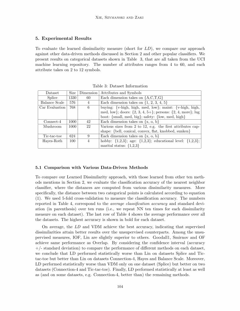
Xie, Szymanski and Zaki
5. Experimental Results
To evaluate the learned dissimilarity measure (short for LD), we compare our approachagainst other data-driven methods discussed in Section 2 and other popular classifiers. Wepresent results on categorical datasets shown in Table 3, that are all taken from the UCImachine learning repository. The number of attributes ranges from 4 to 60, and eachattribute takes on 2 to 12 symbols.
Table 3: Dataset Information
Dataset Size Dimension Attributes and SymbolsSplice 1330 60 Each dimension takes on A,C,T,G
Balance Scale 576 4 Each dimension takes on 1, 2, 3, 4, 5Car Evaluation 768 6 buying: v-high, high, med, low; maint: v-high, high,
med, low; doors: 2, 3, 4, 5+; persons: 2, 4, more; lugboot: small, med, big; safety: low, med, high
Connect-4 1000 42 Each dimension takes on x, o, bMushroom 1000 22 Various sizes from 2 to 12, e.g. the first attributes cap-
shape: bell, conical, convex, flat, knobbed, sunkenTic-tac-toe 624 9 Each dimension takes on x, o, bHayes-Roth 100 4 hobby: 1,2,3; age: 1,2,3; educational level: 1,2,3;
marital status: 1,2,3
5.1 Comparison with Various Data-Driven Methods
To compare our Learned Dissimilarity approach, with those learned from other ten meth-ods mentions in Section 2, we evaluate the classification accuracy of the nearest neighborclassifier, where the distances are computed from various dissimilarity measures. Morespecifically, the distance between two categorical points is calculated according to equation(1). We used 5-fold cross-validation to measure the classification accuracy. The numbersreported in Table 4, correspond to the average classification accuracy and standard devi-ation (in parenthesis) over ten runs (i.e., we repeat NN ten times for each dissimilaritymeasure on each dataset). The last row of Table 4 shows the average performance over allthe datasets. The highest accuracy is shown in bold for each dataset.
On average, the LD and VDM achieve the best accuracy, indicating that superviseddissimilarities attain better results over the unsupervised counterparts. Among the unsu-pervised measures, IOF, Lin are slightly superior to others. Goodall1, Smirnov and OFachieve same performance as Overlap. By considering the confidence interval (accuracy+/- standard deviation) to compare the performance of different methods on each dataset,we conclude that LD performed statistically worse than Lin on datasets Splice and Tic-tac-toe but better than Lin on datasets Connection-4, Hayes and Balance Scale. Moreover,LD performed statistically worse than VDM only on one dataset (Splice) but better on twodatasets (Connection-4 and Tic-tac-toe). Finally, LD performed statistically at least as wellas (and on some datasets, e.g. Connection-4, better than) the remaining methods.
104

Learning Dissimilarities for Categorical Symbols
Table 4: Performance comparison on various dissimilarities
Overlap Lin Smirnov Goodall1 EskinSplice 89.45(0.58) 94.21(0.42) 88.53(0.82) 88.79(0.69) 88.42(0.60)
Balance Scale 75.31(1.44) 75.52(3.31) 74.65(2.14) 75.69(2.04) 64.23(0.51)Car Evaluation 87.86(1.23) 92.64(1.65) 83.72(2.14) 84.96(2.26) 86.65(0.75)
Connect-4 84.20(0.92) 78.25(1.05) 75.30(0.73) 82.50(0.46) 83.55(0.30)Mushroom 100(0) 100(0) 99.75(0.17) 99.90(0.06) 100(0)Tic-tac-toe 81.59(1.56) 98.64(0.69) 84.03(1.07) 86.97(1.58) 63.85(0.93)Hayes-Roth 70.90(4.99) 71.00(3.65) 71.00(5.50) 69.50(5.01) 67.00(5.76)
Avgerage 84.18(1.53) 87.18(1.53) 82.42(1.79) 84.04(1.72) 79.10(1.26)
IOF OF Gambaryan Burnaby VDM LDSplice 90.15(0.62) 88.34(0.68) 88.38(0.67) 83.72(1.19) 95.60(0.57) 93.00(0.67)
Balance Scale 75.86(3.53) 75.34(3.08) 75.17(2.37) 75.43(2.88) 92.10(1.36) 94.04(1.21)Car Evaluation 89.12(1.92) 92.83(0.88) 83.52(2.06) 92.44(0.86) 97.33(1.74) 98.00(1.47)
Connect-4 83.40(0.87) 84.70(0.78) 50.00(0) 85.15(0.84) 83.80(0.96) 87.48(0.92)Mushroom 99.95(0.03) 100(0) 50.00(0) 100(0.09) 100(0) 100(0)Tic-tac-toe 97.13(0.43) 77.48(1.17) 88.85(1.25) 69.27(1.12) 82.15(2.57) 95.30(1.72)Hayes-Roth 68.50(4.67) 58.00(8.25) 75.50(3.52) 57.50(8.30) 73.00(4.70) 79.40(1.71)
Avgerage 86.30(1.72) 82.38(2.12) 73.06(1.41) 80.50(2.18) 89.14(1.70) 92.46(1.10)
5.2 Comparison with Various Classifiers
We consider the NN based on our learned dissimilarity as an “enhanced” nearest neighborclassifier, again denoted as LD. The performance of LD is compared with algorithms imple-mented in Weka 3.6, including decision tree (C4.5 with pruning), Naıve Bayes (NB), RBFneural network (RBFNN, with clustering technique to estimate the number of kernels), andSVM (with RBF kernel and complexity 1.0). Our method uses the learned mapping r,whereas the other methods use the Euclidean distance (corresponding to simple matching)between categorical points. The performance metric is the average classification accuracyover ten runs based on 5-fold cross validation. As shown in Table 5, considering the sameconfidence intervals as in Sec.5.1, we conclude that LD performed statistically worse thanthe other methods on only one dataset (Splice) but performed better on at least three otherdatasets than each of the other methods, which we believe shows a significant improvementover them.
6. Conclusions
In this paper, we propose a task-oriented or supervised iterative learning approach to learna distance function for categorical data. The algorithm explores the relationships betweencategorical symbols by utilizing the classification error as guidance. We show that the realvalue mappings found by our algorithm provide discriminative information, which can beused to refine features and improve classification accuracy. In the future work, we would liketo extend the approach to continuous and mixed attribute datasets, as well as “relational”datasets where there are links between data points.
105

Xie, Szymanski and Zaki
Table 5: Performance comparison on various classifiers
C4.5 NB RBFNN SVM LDSplice 95.03(1.00) 97.01(0.42) 97.01(0.64) 96.91(0.60) 93.00(0.67)
Balance Scale 73.11(1.78) 96.34(1.53) 90.68(1.50) 95.49(1.78) 94.04(1.21)Car Evaluation 96.51(1.12) 92.32(2.33) 93.58(2.01) 88.24(1.88) 98.00(1.47)
Connect-4 87.01(1.71) 87.53(1.10) 88.35(1.62) 87.48(0.89) 87.48(0.92)Mushroom 100(0.00) 97.33(1.00) 100(0.04) 100(0.00) 100(0.00)Tic-tac-toe 85.44(3.26) 76.67(1.94) 80.75(2.53) 77.21(1.27) 95.30(1.72)Hayes-Roth 71.00(8.07) 68.50(9.15) 72.40(5.17) 64.10(12.42) 79.40(1.71)
Average 86.87(2.42) 87.96(2.49) 88.97(1.93) 87.06(2.69) 92.46(1.10)
References
S. Boriah, V. Chandola, and V. Kumar. Similarity measures for categorical data: A com-parative evaluation. In SIAM Data Mining Conference, pages 243–254, 2008.
T. Burnaby. On a method for character weighting a similarity coefficient employing theconcept of information. Mathematical Geology, 2(1):25–38, 1970.
V. Cheng, C.H. Li, and J.T. Kwok. Dissimilarity learning for nominal data. PatternRecognition, 37(7):1471–1477, 2004.
E. Eskin, A. Arnold, and M. Prerau. A geometric framework for unsupervised anomalydetection. Applications of Data Mining in Computer Security, pages 78–100, 2002.
P. Gambaryan. A mathematical model of taxonomy. SSR, 17(12):47–53, 1964.
D. Goodall. A new similarity index based on probability. Biometrics, 22(4):882–907, 1966.
K.S. Jones. A statistical interpretation of term specificity and its application in retrieval.Document Retrieval Systems, 3:132–142, 1988.
M. Liang. Data mining:concepts, models, methods, and algorithms. IIE Transactions, 36(5):495–496, 2004.
D. Lin. An information-theoretic definition of similarity. In 15th International Conferenceon Machine Learning, pages 296–304, 1998.
E. S. Smirnov. On exact methods in systematics. Systematic Zoology, 17(1):1–13, 1968.
C. Stanfill and D. Waltz. Toward memory-based reasoning. CACM, 29:1213–1228, 1986.
106
Related Documents

![AnOverviewof TransferLearning - Nanjing Universitylamda.nju.edu.cn/conf/mlss2014/(X(1)S(kcfwaxyqgaqzl2...JMLR 2009] • Transfer$learning$for$ classificaon,$and$ regression$problems.$](https://static.cupdf.com/doc/110x72/5b05aa8b7f8b9ad1768bb2ef/anoverviewof-transferlearning-nanjing-x1skcfwaxyqgaqzl2jmlr-2009-transferlearningfor.jpg)