JEM Derivation of Locational Marginal Prices - … · Derivation of Locational Marginal Prices for Restructured Wholesale Power Markets Haifeng Liu ... Energy Exemplar PLEXOS® and

Derivation of Locational Marginal Prices for Restructured Wholesale Power Markets

Haifeng Liu California Independent System Operator Corporation, 151 Blue Ravine Road, Folsom, CA

95630, USA; email: [email protected], phone: +1-916-673-7720

Leigh Tesfatsion Department of Economics, Iowa State University, Ames, IA 50011-1070, USA, email:

[email protected], phone: +1-515-294-0138

A. A. Chowdhury California Independent System Operator Corporation, 151 Blue Ravine Road, Folsom, CA

95630, USA; email: [email protected], phone: +1-916-608-1113

2

Executive Summary

Although Locational Marginal Pricing (LMP) plays an important role in many restructured

wholesale power markets, the detailed derivation of LMPs as actually used in industry

practice is not readily available. This lack of transparency greatly hinders the efforts of

researchers to evaluate the performance of these markets. In this paper, different AC and DC

optimal power flow (OPF) models are presented to help understand the derivation of LMPs.

As a byproduct of this analysis, we are able to provide a rigorous explanation of the basic

LMP and LMP-decomposition formulas (neglecting real power losses) presented without

derivation in the business practice manuals of the U.S. Midwest Independent System

Operator (MISO).

Keywords: Locational marginal pricing, wholesale power market, AC optimal power flow,

DC optimal power flow, U.S. Midwest Independent System Operator (MISO).

3

1 INTRODUCTION

In an April 2003 White Paper the U.S. Federal Energy Regulatory Commission (FERC

(2003)) proposed a market design for common adoption by U.S. wholesale power markets.

Core features of this proposed market design include: central oversight by an independent

market operator; a two-settlement system consisting of a day-ahead market supported by a

parallel real-time market to ensure continual balancing of supply and demand for power; and

management of grid congestion by means of Locational Marginal Pricing (LMP), i.e., the

pricing of power by the location and timing of its injection into, or withdrawal from, the

transmission grid.

Versions of FERC’s market design have been implemented (or scheduled for

implementation) in U.S. energy regions in the Midwest (MISO), New England (ISO-NE),

New York (NYISO), the mid-Atlantic states (PJM), California (CAISO), the southwest (SPP),

and Texas (ERCOT). Nevertheless, strong criticism of the design persists (Joskow (2006)).

Part of this criticism stems from the concerns of non-adopters about the suitability of the

design for their regions due to distinct local conditions (e.g., hydroelectric power in the

northwest). Even in regions adopting the design, however, criticisms continue to be raised

about market performance.

One key problem underlying these latter criticisms is a lack of full transparency regarding

market operations under FERC’s design. Due in great part to the complexity of the market

design in its various actual implementations, the business practices manuals and other public

documents released by market operators are daunting to read and difficult to comprehend.

Moreover, in many energy regions (e.g., MISO), data is only posted in partial and masked

form with a significant time delay (Dunn (2007)). The result is that many participants are

wary regarding the efficiency, reliability, and fairness of market protocols (e.g., pricing and

settlement practices). Moreover, university researchers are hindered from subjecting FERC’s

design to systematic testing in an open and impartial manner.

One key area where lack of transparency prevents objective assessments is determination

of LMPs. For example, although MISO’s Business Practices Manual 002 (MISO (2008a))

presents functional representations for LMPs as well as an LMP decomposition for

settlement purposes, derivations of these formulas are not provided. In particular, it is unclear

4

whether the LMPs are derived from solutions to an AC optimal power flow (OPF) problem

or some form of DC OPF approximation. Without knowing the exact form of the

optimization problem from which the LMPs are derived, it is difficult to evaluate the extent

to which pricing in accordance with these LMPs ensures efficient and reliable market

operations.

This paper focuses careful attention on the derivation of LMPs for the operation of

wholesale power markets. Section 2 presents a “full-structured” AC OPF model for LMP

calculation. The LMPs are derived from the full-structured AC OPF model based on the

definition of an LMP and the envelope theorem. Section 3 first derives a “full-structured” DC

OPF model from the full-structured AC OPF model, together with corresponding LMPs. A

“reduced-form” DC OPF model is then derived from the full-structured DC OPF model, and

it is shown that the LMPs derived from the reduced-form DC OPF model are the same as

those derived from the full-structured DC OPF model. As a byproduct of this analysis, we are

able to provide a rigorous explanation of the basic LMP and LMP-decomposition formulas

(neglecting real power losses) presented without derivation in the MISO Business Practices

Manual 002 for Energy Markets. Section 4 concludes.

2 LMP CALCULATION UNDER AC OPF

The concept of an LMP (also called a spot price or a nodal price) was first developed by

Schweppe et al (1998). LMPs can be derived using either an AC OPF model or a DC OPF

model (Momoh et al (1999)).

The AC OPF model is more accurate than the DC OPF model, but it is prone to

divergence. Also, the AC OPF model can be up to 60 times slower than the DC OPF model

(Overbye et al (2004)). The DC OPF model (or the linearized AC OPF model) has been

widely used for LMP calculation for power market operation (Ott (2003) and Litvinov et al

(2004)). Several commercial software tools for power market simulation such as Ventyx

Promod IV®, ABB GridViewTM, Energy Exemplar PLEXOS® and PowerWorld use the DC

OPF model for power system planning and LMP forecasting (Clayton et al (1996); Yang et

al (2003); and Li (2007)).

There are two forms of DC OPF models, “full structured” (Sun et al (2007a) and Sun et

al (2007c)) and “reduced form” (Ilic et al (1998); Shahidehpour et al (2002); Ott (2003);

5

Litvinov et al (2004); Li (2007); and Li et al (2007)). The full-structured DC OPF model has

a real power balance equation for each bus. This is equivalent to imposing a real power

balance equation for all but a “reference” bus, together with a “system” real power balance

equation consisting of the sum of the real power balance conditions across all buses. The

reduced-form DC OPF model solves out for voltage angles using the real power balance

equations at all but the reference bus, leaving the system real power balance equation.

In this paper, real power load and reactive power load are assumed to be fixed and a

particular period of time is taken for the OPF formulations, e.g., an hour. Given a power

system with N buses, ijij jBG + is the thij element of the bus admittance matrix, Y, of the

power system. See Appendix A for the details of the bus admittance matrix. Let the bus

voltage in polar form at bus i be denoted as follows:

iii VV θ∠=•

(1)

where iV denotes the voltage magnitude and iθ denotes the voltage angle.

The N buses are renumbered as follows for convenience:

• Non-reference buses are numbered from 1 to N-1;

• The reference bus is numbered as bus N. Only the differences of voltage angles are

meaningful in power flow calculation. Therefore, following standard practice, the

voltage angle of the reference bus is set to 0.

2.1 Power Balance Constraint

The power flow equations (equality constraints) in the AC OPF problem formulation are as

follows:

[ ] 0)( =−++ ∑∈ kIi

ikkpk pDxf ξ for k=1,…,N (2)

0)( _ =−+ ∑∈ kIi

ikloadqk qQxf for k=1,…,N (3)

Here,

• [ ]T21121 NN VVVx LL −= θθθ is a vector of voltage angles and magnitudes.

• )(xf pk is the real power flowing out of bus k:

6

( ) ( )[ ]∑=

−+−=N

iikkiikkiikpk BGVVxf

1sincos)( θθθθ (4)

• )(xf qk is the reactive power flowing out of bus k:

( ) ( )[ ]∑=

−−−=N

iikkiikkiikqk BGVVxf

1cossin)( θθθθ (5)

• Ik is the set of generators connected to bus k.

• pi is the real power output of generator i.

• Dk is the given real power load at bus k.

• Qload_k is the given reactive power load at bus k.

• qi is the reactive power output of generator i.

• ξk is an auxiliary parameter associated with bus k that is set to zero. Changes in ξk will

later be used to parameterize the real load increase at bus k in order to derive the real

power LMP at bus k.

2.2 Network Constraints

In general, the network constraints for an AC OPF problem formulation include:

• branch (transmission line and transformer) power flow limits, and

• voltage magnitude and angle limits.

The complex power flowing from bus i to bus j on the branch ij is:

22

2

22

2*

~

]][sincos[

]][[

ijij

ijijijjiijjii

ijij

ijijjii

ijij

jii

ijij

jiiijiijijij

xrjxrVjVVVV

xrjxrVVV

jxrVVV

jxrVVVIVjQPS

++−−

=

++−

=−−

=⎥⎥

⎦

⎤

⎢⎢

⎣

⎡

+−

==+=

∗•∗∗•

•••∗•

θθ (6)

where Iij is the current flowing from bus i to bus j, jiij θθθ −= , and rij and xij are the

resistance and reactance of branch ij, respectively. Therefore, the real power flowing from

bus i to bus j is:

22

2 ]sin[]cos[)(

ijij

ijijjiijijjiiij xr

xVVrVVVxP

++−

=θθ

(7)

The reactive power flowing from bus i to bus j is:

7

22

2 ]sin[]cos[)(

ijij

ijijjiijijjiiij xr

rVVxVVVxQ

+−−

=θθ

(8)

The magnitude of the complex power flowing from bus i to bus j is:

)()()()( 22~

xQxPxSxS ijijijij +== (9)

The power system operating constraints include:

Branch power flow constraints: max)(0 ijij SxS ≤≤ for each branch ij (10)

Bus voltage magnitude constraints: maxmin

kkk VVV ≤≤ for k=1,2,…,N (11)

To simplify the illustration, a general form of constraints is used to represent the above

specific inequality constraints (10) and (11), as follows: maxmin )( mmm gxgg ≤≤ for m=1,…,M (12)

2.3 Generator Output Limits

Generator real power output limits for the submitted generator supply offers are assumed to

take the following form: maxminiii ppp ≤≤ Ii∈∀ (13)

Similarly, generator reactive power output limits are assumed to take the following form: maxminiii qqq ≤≤ Ii∈∀ (14)

2.4 Objective Function of the Market Operator

According to MISO’s business practices manuals and tariff (MISO (2005) and MISO

(2008b)), the supply (resource) offer curve of each generator in each hour h must be either a

step function or a piecewise linear curve consisting of up to ten price-quantity blocks, where

the price associated with each quantity increment (MW) gives the minimum price ($/MWh)

the generator is willing to accept for this quantity increment. The blocks must be

monotonically increasing in price and they must cover the full real-power operating range of

the generator.

8

Let Ci(pi) denote the integral of generator i’s supply offer from pimin to pi. For simplicity

of illustration, Ci(pi) will hereafter be assumed to be strictly convex and non-decreasing over

a specified interval.

In this study the Independent System Operator (ISO) is assumed to solve a centralized

optimization problem in each hour h to determine real power commitments and LMPs for

hour h conditional on the submitted generator supply offers and given loads (fixed demands)

for hour h; price-sensitive demand bids are not considered. As will be more carefully

explained below, this constrained optimization problem is assumed to involve the

minimization of total reported generator operational costs defined as follows:

∑∈Ii

ii pC )( (15)

where Ci(pi) is generator i’s reported total costs of supplying real power pi in hour h, and I is

the set of generators. Since for each generator supply offer the unit of the incremental energy

cost is $/MWh and the unit of the operating level is MW, the unit of the objective function

(15) is $/h.

2.5 AC OPF Problem

The overall optimization problem is as follows:

∑∈Ii

iixqppC

ii

)(min,,

(16)

s.t.

Real power balance constraints for buses k=1,…,N:

[ ] 0)( =−++ ∑∈ kIi

ikkpk pDxf ξ (17)

Reactive power balance constraints for buses k=1,…,N:

0)( _ =−+ ∑∈ kIi

ikloadqk qQxf (18)

Power system operating constraints for m=1,..,M: maxmin )( mmm gxgg ≤≤ (19)

Generator real power output constraints for generators Ii∈ : maxminiii ppp ≤≤ (20)

9

Generator reactive power output constraints for generators Ii∈ : maxminiii qqq ≤≤ (21)

The endogenous variables are pi, qi and x. The exogenous variables are ξk, Dk and Qload_k.

The above optimization problem is also called the AC OPF problem.

2.6 LMP Calculation Based on AC OPF Model

The Lagrangian function for the AC OPF problem is as follows:

[ ]

[ ]

[ ]

[ ]

[ ]

[ ] limitlower output power reactiveGenerator

limitupper output power reactiveGenerator

limitlower output power realGenerator

limitupper output power realGenerator

limitlower constraint operating systemPower )(

limitupper constraint operating systemPower )(

constraintbalancepower Reactive)(

constraintbalancepower Active)(][

cost Total)(

min

max^

min

max^

1

min

1

max^

1_

1

∑

∑

∑

∑

∑

∑

∑ ∑

∑ ∑

∑

∈

∨

∈

∈

∨

∈

=

∨

=

= ∈

= ∈

∈

−−

−−

−−

−−

−−

−−

⎥⎦

⎤⎢⎣

⎡+−−−

⎥⎦

⎤⎢⎣

⎡+−+−−

=

Iiiii

Iiiii

Iiiii

Iiiii

M

mmmm

M

mmmm

N

k Iiikloadqkk

N

k Iiipkkkk

Iiii

qq

qq

pp

pp

gxg

xgg

qQxf

pxfD

pCl

k

k

ω

ω

τ

τ

μ

μ

λ

ξπ

(22)

DEFINITION 2.1 (LMP) The Locational Marginal Price (LMP) of electricity at a location

(bus) is defined as the least cost to service the next increment of demand at that location

consistent with all power system operating constraints (MISO (2005) and CAISO (2006)).

Assume the above AC OPF problem has an optimal solution, and assume the minimized

objective function J*(exogenous variables) is a differentiable function of ξk for each k =

1,...,N. Using the envelope theorem (Varian (1992)), the LMP at each bus k can then be

calculated as follows:

10

kkk

kJLMP πχ

ξξ=

∂∂

=∂∂

= ** l , for k=1, 2, .., N (23)

Here,

• J* is the minimized value of the total cost objective function (15), also referred to as

the indirect objective function or optimal value function.

• χ* is the solution vector consisting of the optimal values for the decision variables.

It follows from (23) that the real power LMP at each bus k is simply the Lagrange

multiplier associated with the real power balance constraint for that bus.

3 LMP CALCULATION AND DECOMPOSITION UNDER DC OPF

3.1 DC OPF Approximation in Full-Structured Form

The AC OPF model involves real and reactive power flow balance constraints and power

system operating constraints, which constitute a set of nonlinear algebraic equations. It can

be time consuming to solve AC OPF problems for large power systems, and convergence

difficulties can be serious. The DC OPF model has been proposed to approximate the AC

OPF model for the purpose of calculating real power LMPs (Overbye et al (2004)).

In the DC OPF formulation, the reactive power flow equation (3) is ignored. The real

power flow equation (2) is approximated by the DC power flow equations under the

following assumptions (Wood et al (1996); Kirschen et al (2004); Overbye et al (2004); and

Sun et al (2007b)):

a) The resistance of each branch rkm is negligible compared to the branch reactance xkm

and can therefore be set to zero.

b) The bus voltage magnitude is equal to one per unit.1

1 In power system calculations quantities such as voltage, current, power and impedance are usually expressed in per unit (p.u.) form, i.e., as a percentage of a specified base value. The p.u. quantity is calculated as the actual quantity divided by the base value of quantity where the actual quantity is the value of the quantity in the actual units. The base value has the same units as the actual quantity. Thus p.u. quantity is dimensionless. Specifying two independent base quantities determines the remaining base quantities. The two independent quantities are usually taken to be base voltage and base apparent power. Manufacturers usually specify the impedances of machines and transformers in p.u. The advantages of the p.u. system include: (a) simplification of the transformer equivalent circuit, (b) allowance of rapid checking of p.u. impedance data for gross errors, and (c) reduction of the chances of numerical instability. For a detailed and careful discussion of base value determinations and p.u. calculations, see Chapter 5 of Bergen et al (2000).

11

c) The voltage angle difference mk θθ − across any branch is very small so that

1)cos( ≈− mk θθ and mkmk θθθθ −≈− )sin( .

Purchala et al. (2005) show that the resulting DC OPF model is acceptable in real power

flow analysis if the branch power flow is not very high, the voltage profile is sufficiently flat,

and the rkm/xkm ratio is less than 0.25. The DC OPF model itself does not include the effect of

the real power loss on the LMP due to assumption a). Li et al. (2007) propose an iterative

approach to account for the real power loss in the DC OPF-based LMP calculation. In the

present study, however, real power loss is neglected in conformity with standard DC OPF

treatments.

From (2) and (4) we have:

[ ] 0)sin()cos(1

=−+−+− ∑∑∈= kIi

ik

N

mmkkmmkkmmk pDBGVV θθθθ for k=1…N (24)

where, as explained in Appendix A, Gkm and Bkm are elements of the bus admittance matrix.

Given assumption a), it follows that 022 =+

−=kmkm

kmkm xr

rG for mk ≠ ,

0,1

2220

20

0 =+

++

= ∑≠=

N

Nmm kmkm

km

kk

kkk xr

rxr

rG and kmkmkm

kmkm xxr

xB 122 =

+= for mk ≠ , ∑

= +−

=N

m kmkm

kmkk xr

xB1

22 .

Given assumption b), it follows that Vk = Vm = 1. Given assumption c), it follows that

mkmk θθθθ −≈− )sin( . Therefore, (24) reduces to:

0)(1,1

=−+⎥⎦

⎤⎢⎣

⎡− ∑∑

∈≠= kIiik

N

kmmmk

km

pDx

θθ for k=1…N (25)

Equation (25) can be reexpressed as:

kk

N

kmmmk

km

DPx

−=⎥⎦

⎤⎢⎣

⎡−∑

≠= ,1

)(1 θθ for k=1…N (26)

Therefore, the net injection Pk – Dk of real power flowing out of any bus k can be

approximated as a linear function of the voltage angles.

From (7), the real power flowing from bus k to bus m is as follows:

22

2 ]sin[]cos[)(kmkm

kmkmmkkmkmmkkkm xr

xVVrVVVxP++−

=θθ (27)

Based on the assumptions a), b) and c),

12

km

mkkm x

xP θθ −=)( (28)

Therefore, this branch real power flow can be approximated as a linear function of the

voltage angle difference between bus k and bus m.

From (8), the reactive power flowing from bus k to bus m is as follows:

22

2 ]sin[]cos[)(kmkm

kmkmmkkmkmmkkkm xr

rVVxVVVxQ+

−−=

θθ (29)

Based on the assumptions a), b) and c),

0)( =xQkm (30) From (9), the magnitude of the complex power flow Skm(x) is:

)()()()( 222 xPxQxPxS kmkmkmkm =+= (31) Therefore, the branch power flow constraint becomes:

maxmin )( kmkmkm FxPF ≤≤ (32) There are no voltage magnitude constraints because all voltage magnitudes are assumed

to be 1.0 p.u.

For a power system consisting of N buses, the DC power flow equation for each bus k is

shown in (26). The corresponding matrix form for the full system of equations is as follows:

θBDP =− (33) Here,

• TNPPP ][ 21 L=P is the 1×N vector of nodal real power generation for buses 1, …,N.

• TNDDD ][ 21 L=D is the 1×N vector of nodal real power load for buses 1, …,N.

• B is an NN × matrix (independent of voltage angles) that is determined by the

characteristics of the transmission network as follows: ∑=m

kmkk xB /1 for each

diagonal element kk, and kmkm xB /1−= for each off-diagonal element km.

• TN ][ 21 θθθθ L= is the 1×N vector of voltage angles for buses 1, …, N.

The system of equations (33) is called the full-structured DC power flow model.

The voltage angle at the reference bus N is usually normalized to zero since the real

power balance constraints and real power flow on any branch are only dependent on voltage

angle differences, as seen from (26) and (28). We follow this convention here, therefore:

13

0=Nθ (34) Given (34), the system of real power balance equations for buses 1, …, N-1 (33) can be

expressed in reduced matrix form as follows: '''' θBDP =− (35)

Here,

• TNPPP ][ 121

'−= LP is the 1)1( ×−N vector of real power generation for buses 1, …,

N-1.

• TNDDD ][ 121

'−= LD is the 1)1( ×−N vector of real power load for buses 1, …, N-1.

• 'B is the “B-prime” matrix of dimension )1()1( −×− NN , independent of voltage

angles, that is determined by the characteristics of the transmission network. The B'

matrix is derived from the B matrix by omitting the row and column corresponding to

the reference bus.

• TN ][ 121

'−= θθθθ L is the 1)1( ×−N vector of voltage angles for buses 1, …, N-1.

For later reference, it follows from (B.16) in Appendix B that the real power balance

equation at the reference bus N can be expressed as follows:

][ '' DPe −−=− TNN DP (36)

Here,

• ]111[ L=Te is an )1(1 −× N row vector with each element equal to 1.

In the DC OPF model, the real power flow on any branch km is given in (28). Letting M

denote the total number of distinct transmission network branches for the DC OPF model, it

follows that the real power flow on all M branches can be written in a matrix form as follows:

θXF = (37) Here,

• TM xFxFxF )]()()([ 21 L=F is the 1×M vector of branch flows.

• AHX ×= is a NM × matrix, which is determined by the characteristics of the

transmission network.

• H is an MM × matrix whose non-diagonal elements are all zero and whose kkth

diagonal element is the negative of the susceptance of the kth branch.

14

• A is the NM × adjacency matrix. It is also called the node-arc incidence matrix, or

the connection matrix. See Appendix C for the details of the development of the

adjacency matrix A.

Inverting (35) yields:

][][ ''1'' DPB −= −θ (38) Substitution of (38) into (37) yields:

][000

000

0][ 1'''1'''1''

DPB

XDPB

XDPB

XXXF −⎥⎦

⎤⎢⎣

⎡=⎥

⎦

⎤⎢⎣

⎡

−−

⎥⎦

⎤⎢⎣

⎡=⎥

⎦

⎤⎢⎣

⎡ −=⎥

⎦

⎤⎢⎣

⎡==

−−−

NNn DPθθ

θ (39)

Let

⎥⎦

⎤⎢⎣

⎡=

−

0001'B

XT (40)

Here,

• T is a NM × matrix.

• TmN = 0 for m=1, …, M.

Therefore, the branch power flows in terms of bus net real power injections can be

expressed as:

][ DPTF −= (41)

The system of equations (41) is called the reduced-form DC power flow model because it

directly relates branch real power flows to bus net real power injections.

The real power flow on branch l in (41) is as follows:

[ ] [ ]kk

N

klkkk

N

klkl DPTDPTF −=−= ∑∑

−

==

1

11 for l=1, …, M (42)

Assume Pk is increased to kk PP Δ+ while P1, P2, …, Pk-1, Pk+1, …, PN-1 and D1, D2, …,

DN remain fixed. Then, according to (42), the increase in the real power flow on branch l,

lFΔ , is as follows:

klkl PTF Δ=Δ (43) By (36), note that the change in the real power injection at bus k is exactly compensated

by an opposite change in the real power injection at the reference bus N, given by kN PP Δ− .

Therefore, Tlk in (43) is a generation shift factor.

15

More precisely, it is clear from (39) that the branch power flows are explicit functions of

nodal net real power injections (generation less load) at the non-reference buses. It follows

from (36) that the generation change at bus k will be compensated by the generation change

at the reference bus N assuming the net real power injections at other buses remain constant.

Thus, the lkth element Tlk in the matrix T in (41) is equal to the generation shift factor alk as

defined on page 422 of Wood et al (1996), which measures the change in megawatt power

flow on branch l when one megawatt change in generation occurs at bus k compensated by a

withdrawal of one megawatt at the reference bus.

The full-structured DC OPF model is derived from the full-structured AC OPF model in

Section 2 based on the three assumptions a), b), and c) in Section 3.1, as follows:

∑∈Ii

iippC

ki

)(min,θ

(44)

s.t.

Real power balance constraint for each bus Nk ,,1L= :

[ ] ∑∑≠=∈

⎥⎦

⎤⎢⎣

⎡−=+−

N

kmmmk

kmkk

Iii x

Dpk ,1

)(1 θθξ for k=1…N (45)

Real power flow constraints for each distinct branch km :

max][1kmmk

km

Fx

≤−θθ (46)

min][1kmmk

km

Fx

≥−θθ (47)

Real power generation constraints for each generator: maxminiii ppp ≤≤ Ii∈∀ (48)

The endogenous variables are pi and θ. The exogenous variables are Dk and ξk.

The optimal solution is determined for the particular parameter values kξ = 0 in (45).

Changes in these parameter values are used below to generate LMP solution values using

envelope theorem calculations.

The Lagrangian function for the optimization problem is:

16

∑

∑

∑

∑

∑ ∑∑

∑

∈

∨

∈

∧

∨

∧

= ≠=∈

∈

−−

−−

−−−

−−−

⎥⎦

⎤⎢⎣

⎡+−⎥

⎦

⎤⎢⎣

⎡−−−

=

Iiiii

Iiiii

kmmkkmkm

km

mkkm

kmkm

km

N

kkk

N

kmmmk

kmIiik

Iiii

pp

pp

Fx

xF

Dx

p

pC

k

)(

)(

]][1[

]][1[

][)(1

)(

min

max

min

max

1 ,1

τ

τ

θθμ

θθμ

ξθθπ

l

(49)

Assume the above DC OPF problem has an optimal solution and the optimized objective

function J*(exogenous variables) is a differentiable function of ξk for each k = 1,...,N. Based

on the envelope theorem and using the auxiliary parameter ξk, we can calculate the LMP at

each bus k as follows:

kkk

kJLMP πχ

ξξ=

∂∂

=∂∂

= ** l , k∀ (50)

It follows from (50) that the LMP at each bus k is the Lagrange multiplier corresponding

to the real power balance constraint at bus k, evaluated at the optimal solution.

As depicted in Figure 1, we use a three-bus system with two generators and one fixed

load to illustrate LMP calculations based on the full-structured DC OPF model. For the

purpose of illustration, assume: 1) the reactance of each branch is equal to 1 p.u.; 2) the

capacity of branch 2-1 is 50 MW; 3) there are no capacity limits on branches 2-3 and 3-1; 4)

the demand at Bus 1 is fixed at 90 MW; 5) the real power operating capacity limit for

generator 2 and for generator 3 is 100 MW; 6) the indicated marginal costs $5/MWh and

$10/MWh for Generator 2 and Generator 3 are constant over their real power operating

capacity ranges; 7) the time period assumed for the DC-OPF formulation is one hour; and 8)

the objective of the market operator is the constrained minimization of the total variable

costs of operation ($/h), i.e., the summation of the variable costs of operation (marginal cost

times real power generation) for Generator 2 and Generator 3.

17

FIGURE 1 A three-bus power system.

Powe

r flo

w lim

it 50

MW

In the following calculations, all power amounts (generator outputs, load demand, and

branch flows) and impedances are expressed in per unit (p.u.). The base power is chosen to

be 100 MW. The objective function for the DC OPF problem is expressed in per unit terms

as well as the constraints. The variable cost of each generator i is expressed as a function of

per unit real power PGi, i.e., as100×MCi×PGi, where MCi denotes the marginal cost of

Generator i. Note that the per unit-adjusted total variable cost function is then still measured

in dollars per hour ($/h).

Given the above assumptions, the market operator’s optimization problem is formulated

as follows:

32,,,1000500min

3221GGPP

PPGG

+θθ

(51)

s.t.

⎥⎥⎥

⎦

⎤

⎢⎢⎢

⎣

⎡−=

⎥⎥⎥

⎦

⎤

⎢⎢⎢

⎣

⎡

⎥⎥⎥

⎦

⎤

⎢⎢⎢

⎣

⎡

−−−−−−

3

22

1 9.0

0211121112

G

G

PPθ

θ (52)

⎥⎥⎥

⎦

⎤

⎢⎢⎢

⎣

⎡

≤⎥⎥⎥

⎦

⎤

⎢⎢⎢

⎣

⎡

⎥⎥⎥

⎦

⎤

⎢⎢⎢

⎣

⎡

−−−

≤⎥⎥⎥

⎦

⎤

⎢⎢⎢

⎣

⎡

max23

max31

max21

2

1

min23

min31

min21

0110101011

FFF

FFF

θθ

(53)

⎥⎦

⎤⎢⎣

⎡≤⎥

⎦

⎤⎢⎣

⎡≤⎥

⎦

⎤⎢⎣

⎡11

00

3

2

G

G

PP

(54)

18

The solution to this optimization problem yields the following scheduled power

commitments for Generators 2 and 3 and LMP values for Buses 1 through 3:

• PG2 = 0.6 p.u. = 60 MW, PG3 = 0.3 p.u. = 30 MW

• LMP1 = $15/MWh, LMP2 = $5/MWh, LMP3 = $10/MWh

The power flow on branch 2-1 is 50 MW, which is at the capacity limit of the branch. The

power flow on branch 2-3 is 10 MW, and the power flow on branch 3-1 is 40 MW. Figure 2

depicts these results.

FIGURE 2 LMPs, generator scheduled power commitments, and branch power flows.

Load 90 MW

Generation 60 MW Generation 30 MW

Bus 3(Reference bus)

LMP2 = $5/MWh

LMP1 = $15/MWh

LMP3 = $10/MWh

Power flow 10 MW

Bus 2

Bus 1

Recall that the LMP at a location (bus) of a transmission network is defined to be the

minimal additional system cost required to supply an additional increment of electricity to

this location. We now verify that the LMP solution values indicated in Figure 2 indeed

satisfy the definition of an LMP.

Consider Bus 2, which currently has 0 load. Suppose an additional megawatt of load is

now required at Bus 2. It is clear that this additional load should be supplied by Generator 2.

This follows because the marginal cost of Generator 2 is lower than the marginal cost of

Generator 3 and the current output (60MW) of Generator 2 is strictly lower than its operating

capacity limit (100MW). The transmission network has no impact on the LMP at Bus 2

19

because the additional megawatt of power is produced and consumed locally. The LMP at

Bus 2 is therefore $5/MWh, which is equal to the marginal cost of Generator 2.

Determination of the LMP values at Buses 3 and 1 is more complicated because network

externalities are involved. Consider, first, the most efficient way to supply an additional

megawatt of power at Bus 3. This additional megawatt of power cannot be provided by

Generator 2, although it has the lowest marginal cost and is not at maximum operating

capacity, because this would overload branch 2-1. The next cheapest option is to increase the

output of Generator 3. Because Generator 3 is located at Bus 3, the additional megawatt of

power will not flow through the transmission network. The LMP at bus 3 is therefore

$10/MWh, which is equal to the marginal cost of Generator 3.

Consider, instead, the most efficient way to supply an additional MW of power at Bus 1.

It is not feasible to do this by increasing the output of Generator 2 alone, or by increasing the

output of Generator 3 alone, because either option would overload branch 2-1. The only

feasible option is to simultaneously increase the output of Generator 3 and decrease the

output of Generator 2. The required changes in the outputs of Generator 2 and Generator 3

can be calculated by solving the following equations:

ΔPG2 + ΔPG3 = 1 MW (55) (2/3)ΔPG2 + (1/3)ΔPG3 = 0 MW (56)

where (56) is Kirchhoff’s circuit laws applied to the 3-bus system at hand, for which the

reactance on each branch is assumed to be equal. Solving these two equations, we get

ΔPG2 = -1 MW

ΔPG3 = 2 MW

Supplying at minimum cost an additional megawatt of power at Bus 1 therefore requires

that we increase the output of Generator 3 by 2 MW and reduce the output of Generator 2 by

1 MW. The system cost of supplying this megawatt, and hence the LMP at Bus 1, is thus

given by

LMP1 = 2×MC3 – 1×MC2 = 2($10/MWh) – 1($5/MWh) = $15/MWh

In summary, we observe from this three-bus system illustration that

• The MC of Generator 2 determines the LMP of $5/MWh at Bus 2.

• The MC of Generator 3 determines the LMP of $10/MWh at Bus 3.

20

• A combination of the MCs for Generators 2 and 3 determines the LMP of $15/MWh at

Bus 1.

3.2 DC OPF Approximation in Reduced Form

The reduced-form DC OPF model can be derived directly from the full-structured DC

OPF model in Section 3.1 by applying the following three steps:

1) Replace the real power balance equation at the reference bus N by the sum of the real

power balance equations across all N buses. This is an equivalent formulation that will

not change the optimal solution of the DC OPF problem. Since there is no real power loss

in the DC power flow model, the sum of the net real power injections across all buses is

equal to zero; see (B.16) in Appendix B. Therefore, the system real power balance

constraint (in parameterized form) can be expressed as in (58), below.

2) Solve the voltage angles at the N-1 non-reference buses as functions of the net real

power injections at the N-1 non-reference buses as shown in (38).

3) Replace the voltage angles in the branch flow constraints as functions of the net real

power injections at the non-reference buses as shown in (39) and (42).

Since the above transformation is based on equivalency and only eliminates internal

variables (i.e. voltage angles at non-reference buses), the optimal solution and the

corresponding Lagrange multipliers of the branch power flow constraints are the same for the

two DC OPF models.

The resulting reduced-form DC OPF model is then as follows:

∑∈Ii

iippC

i

)(min (57)

s.t.

System real power balance constraint:

0))((1

=+−∑=

N

kkkk DP ξ , where ∑

∈

=kIi

ik pP (58)

Branch real power flow constraint for each branch l:

[ ] max1

1lkkk

N

klk FDPT ≤−−∑

−

=

ξ for l=1, …, M (59)

[ ]kkk

N

klkl DPTF ξ−−≤ ∑

−

=

1

1

min for l=1, …, M (60)

21

Real power output constraint for each generator i: maxminiii ppp ≤≤ Ii∈∀ (61)

The Lagrangian function for this optimization problem is:

[ ]

[ ]

[ ]

[ ]

[ ]∑

∑

∑∑

∑∑

∑

∑

∈

∨

∈

∧

−

==

∨

−

==

∧

=

∈

−−

−−

⎥⎦

⎤⎢⎣

⎡−−−−

⎥⎦

⎤⎢⎣

⎡−−−−

−−−

=

Iiiii

Iiiii

lkkk

N

klk

M

ll

kkk

N

klkl

M

ll

N

kkkk

Iiii

pp

pp

FDPT

DPTF

DP

pC

min

max

min1

11

1

1

max

1

1

)(

τ

τ

ξμ

ξμ

ξπ

l

(62)

Assume the reduced-form DC OPF problem has been solved. Based on the envelope

theorem, using the auxiliary parameter ξk, we can calculate the LMPs for all buses as follows:

kN

M

llkl

M

llkl

kkk TTJLMP MCCMEC

11

**

+=+−=∂∂

=∂∂

= ∑∑=

∨

=

∧

μμπχξξl , Nk ≠∀ (63)

Nkk

kJLMP MEC*

*

==∂∂

=∂∂

= πχξξl , Nk = (64)

Here,

• π=NMEC is the LMP component representing the marginal cost of energy at the

reference bus N.

• ∑∑=

∨

=

∧

+−=M

llkl

M

llklk TT

11

MCC μμ is the LMP component representing the marginal cost of

congestion at bus k relative to the reference bus N.

The derived marginal cost of energy MEC in (63) and (64) is the same as that in (4-1) and

(4-2) on page 35 of the MISO’s Business Practices Manual for Energy Markets (MISO

(2008a)). Recall that Tlk is equal to the Generation Shift Factor (GSFlk), which measures the

change in megawatt power flow on flowgate (branch) l when one megawatt change in

generation occurs at bus k compensated by a withdrawal of one megawatt at the reference

22

bus. From (62), ll

∨∧

− μμ is the Flowgate Shadow Price (FSPl) on flowgate l, which is equal to

the reduction in minimized total variable cost that results from an increase of 1 MW in the

capacity of the flowgate l. Therefore, the marginal congestion component MCC can be

expressed as,

∑=

×−=M

lllkk

1FSPGSFMCC (65)

The derived marginal cost of congestion MCC in (65) is the same as that in (4-3) on page

36 of the MISO’s Business Practices Manual for Energy Markets (MISO (2008a)).

In the following example, we use the same three-bus system as in Section 3.1 to illustrate

the calculation of LMP solution values based on the reduced-form DC OPF model. First, the

optimization problem is formulated as follows:

32,1000500min

32GGPP

PPGG

+ (66)

s.t.

09.032 =−+ GG PP (67)

⎥⎥⎥

⎦

⎤

⎢⎢⎢

⎣

⎡

≤⎥⎥⎥

⎦

⎤

⎢⎢⎢

⎣

⎡−

⎥⎥⎥

⎦

⎤

⎢⎢⎢

⎣

⎡−−

−≤

⎥⎥⎥

⎦

⎤

⎢⎢⎢

⎣

⎡

max23

max31

max21

3

2min

23

min31

min21 9.0

03/23/103/13/203/13/1

FFF

PP

FFF

G

G (68)

⎥⎦

⎤⎢⎣

⎡≤⎥

⎦

⎤⎢⎣

⎡≤⎥

⎦

⎤⎢⎣

⎡11

00

3

2

G

G

PP

(69)

The optimal real power commitments for Generators 2 and 3 are the same as those

obtained for the full-structured DC OPF model:

• PG2 = 0.6 p.u. = 60 MW, PG3 = 0.3 p.u. = 30 MW

The Lagrange multiplier corresponding to the system real power balance constraint, π, is

$10/MWh and the Lagrange multiplier corresponding to the inequality constraint for branch

2-1, μ, is $15/MWh. The LMPs can then be calculated based on (63) and (64) as

LMP1 = MEC3 + MCC1 = π – μ(T11) = 10 – 15(-1/3) = $15/MWh (70) LMP2 = MEC3 + MCC2 = π – μ(T12) = 10 – 15(1/3) = $5/MWh (71)

LMP3 = MEC3 = π = $10/MWh (72) These LMP solution values are the same as those obtained using the full-structured DC

OPF model. Moreover, the marginal cost of congestion at Bus 1 relative to the reference Bus

23

3, MCC1, is $5/MWh, and the marginal cost of congestion at Bus 2 relative to the reference

Bus 3, MCC2, is -$5/MWh.

Consider, instead, the calculation of the shadow price of branch 2-1 directly from its

definition. Recall that the shadow price of a branch is the reduction in minimized total

variable cost that results from an increase of 1 MW in the capacity of the branch. For the

example at hand, suppose the capacity of branch 2-1 is increased by 1 MW. Then the

minimized total variable cost can be reduced by simultaneously increasing the output of

Generator 2 and decreasing the output of Generator 3, since the marginal cost of Generator 2

is less than the marginal cost of Generator 3. The required changes in the outputs of

Generator 2 and Generator 3 can be calculated by solving the following equations:

ΔPG2 + ΔPG3 = 0 MW (73) (2/3)ΔPG2 + (1/3)ΔPG3 = 1 MW (74)

Solving these equations, we get

ΔPG2 = 3 MW

ΔPG3 = -3 MW

Therefore the shadow price of branch 2-1, μ, is

μ = 3($10/MWh – $5/MWh) = $15/MWh.

4 CONCLUSION

Locational marginal pricing plays an important role in many recently restructured wholesale

power markets. Different AC and DC optimal power flow models are carefully presented and

analyzed in this study to help understand the determination of LMPs. In particular, we show

how to derive the full-structured DC OPF model from the full-structured AC OPF model, and

the reduced-form DC OPF model from the full-structured DC OPF model. Simple full-

structured and reduced-form DC OPF three-bus system examples are presented for which the

LMP solutions are first derived using envelope theorem calculations and then derived by

direct definitional reasoning. We also use these examples to illustrate that LMP solution

values derived for the full-structured DC OPF model are the same as those derived for the

reduced-form DC OPF model. As a byproduct of this analysis, we are able to provide a

rigorous explanation of the basic LMP and LMP-decomposition formulas (neglecting real

24

power losses) presented without derivation in the MISO Business Practices Manual 002 for

Energy Markets.

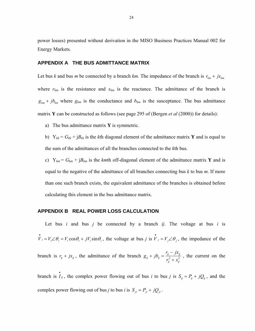
APPENDIX A THE BUS ADMITTANCE MATRIX

Let bus k and bus m be connected by a branch km. The impedance of the branch is kmkm jxr +

where rkm is the resistance and xkm is the reactance. The admittance of the branch is

kmkm jbg + where gkm is the conductance and bkm is the susceptance. The bus admittance

matrix Y can be constructed as follows (see page 295 of (Bergen et al (2000)) for details):

a) The bus admittance matrix Y is symmetric.

b) Ykk = Gkk + jBkk is the kth diagonal element of the admittance matrix Y and is equal to

the sum of the admittances of all the branches connected to the kth bus.

c) Ykm = Gkm + jBkm is the kmth off-diagonal element of the admittance matrix Y and is

equal to the negative of the admittance of all branches connecting bus k to bus m. If more

than one such branch exists, the equivalent admittance of the branches is obtained before

calculating this element in the bus admittance matrix.

APPENDIX B REAL POWER LOSS CALCULATION

Let bus i and bus j be connected by a branch ij. The voltage at bus i is

iiiiiii jVVVV θθθ sincos +=∠=•

, the voltage at bus j is jjj VV θ∠=•

, the impedance of the

branch is ijij jxr + , the admittance of the branch 22ijij

ijijijij xr

jxrjbg

+−

=+ , the current on the

branch is ijI•

, the complex power flowing out of bus i to bus j is ijijij jQPS += , and the

complex power flowing out of bus j to bus i is jijiji jQPS += .

25

The real and reactive power loss along the transmission line ij is2:

ijijijijijijijijijijijijjiijlossijloss xjIrIjxrIIjxrIIVVjQP 222__ ][]][[][ +=+=+=−=+

∗•∗••

(B.1)

where ijI*

is the complex conjugate of ijI•

. Therefore, the real power loss on the transmission

line ij is:

ijijijloss rIP 2_ = (B.2)

Since:

ijij

jiij

jxrVVI

+−

=••

•

(B.3)

The magnitude of the current ijI•

is

22

22 ]sinsin[]coscos[

ijij

jjiijjiiijij

xr

VVVVII

+

−+−==

• θθθθ (B.4)

Therefore:

22

222 cos2

ijij

ijjijiij xr

VVVVI

+−+

=θ

(B.5)

Therefore:

ijijij

ijjijiijijijloss r

xrVVVV

rIxP 22

222

_

cos2)(

+−+

==θ

(B.6)

where the elements of the state vector x are the N-1 voltage angles for the N-1 non-reference

buses and the N voltage magnitudes for all N buses.

The complex power flowing from bus i to bus j is:

2 See (2.18), (2.19) and (2.20) in Section 2.2 of Bergen et al (2000) for the basic principles of complex power supplied to a one-port.

26

22

2

22

2*

]][sincos[

]][[

ijij

ijijijjiijjii

ijij

ijijjii

ijij

jii

ijij

jiiijiijijij

xrjxrVjVVVV

xrjxrVVV

jxrVVV

jxrVVVIVjQPS

++−−

=

++−

=−−

=⎥⎥

⎦

⎤

⎢⎢

⎣

⎡

+−

==+=

∗•∗∗•

•••∗•

θθ (B.7)

where jiij θθθ −= . From (B.7) we have the real power flowing from bus i to bus j:

22

2 ]sin[]cos[)(

ijij

ijijjiijijjiiij xr

xVVrVVVxP

++−

=θθ

(B.8)

From (B.7), the reactive power flowing from bus i to bus j is:

22

2 ]sin[]cos[)(

ijij

ijijjiijijjiiij xr

rVVxVVVxQ

+−−

=θθ

(B.9)

The real power flowing out of bus j to bus i is:

22

2 ]sin[]cos[)(

ijij

ijjijiijijjijji xr

xVVrVVVxP

++−

=θθ

(B.10)

Therefore:

22

22 ]cos2[)()(

ijij

ijijjijijiij xr

rVVVVxPxP

+−+

=+θ

(B.11)

From (B.6) and (B.11), we have

)()()(_ xPxPxP jiijijloss += (B.12)

implying that the loss on each transmission line ij is a function of the state vector x.

The total system real power loss, which is the sum of the real power loss along each

transmission line ij, is then given by:

∑ ∑∑=

=+==ij

N

ipijiij

ijijlosssysloss xfxPxPxPxP

1__ )()]()([)()( (B.13)

27

where N is the total number of buses and )(xf pi is the total real power flowing out of bus i.

The latter expression denotes the sum of all the real power flowing out of the ith bus along

the transmission lines connected to the ith bus, which can be represented as follows:

( )∑=

−+−=n

kkiikkiikkipi BGVVxf

1)sin()cos()( θθθθ (B.14)

where Gik+jBik is the ikth element of the bus admittance matrix Y.

If branch resistance is neglected, i.e., if we set 0=ijr for each transmission line ij, then

from (B.2) we have:

02_ == ijijijloss rIP (B.15)

for each ij. From (B.13) we then have:

[ ] 0)()( _11

===− ∑∑∑==

xPxfDPij

ijloss

N

ipi

N

iii (B.16)

APPENDIX C ADJACENCY MATRIX

The row-dimension of the adjacency matrix A is equal to M, the number of branches, and the

column-dimension of A is equal to N, the number of buses. The kjth element of A is 1 if the

kth branch begins at bus j, -1 if the kth branch terminates at bus j, and 0 otherwise. A branch k

connecting a bus j to a bus i is said to “begin” at bus j if the power flowing across branch k is

defined positive for a direction from bus j to bus i. Conversely, branch k is said to

“terminate” at bus j if the power flowing across branch k is defined positive for a direction to

bus j from bus i.

28

REFERENCES Bergen, A. R. and Vittal, V. (2000). Power System Analysis, Second Edition. Prentice Hall,

New Jersey.

CAISO. (2006). CAISO Tariff Appendix A: Master Definitions Supplement.

http://www.caiso.com/1b93/1b936f946ff90.html

Clayton, R. E. and Mukerji, R. (1996). System planning tools for the competitive market.

IEEE Computer Applications in Power 9, 50-55.

Dunn, W. H., Jr. (2007). Data required for market oversight.

http://www.appanet.org/files/PDFs/dunn2007.pdf

Ilic, M., Galiana, F., and Fink, L. (1998). Power System Restructuring: Engineering and

Economics. Kluwer, Norwell.

Joskow, P. (2006). Markets for power in the United States: An interim assessment. The

Energy Journal 27, 1-36.

Kirschen, D. and Strbac, G. (2004). Fundamentals of Power System Economics. John Wiley

& Sons, Ltd., Chichester.

Li, F. (2007). Continuous locational marginal pricing (CLMP). IEEE Transactions on Power

Systems 22, 1638-1646.

Li, F. and Bo, R. (2007). DCOPF-based LMP simulation: algorithm, comparison with

ACOPF, and sensitivity. IEEE Transactions on Power Systems 22, 1475-1485.

Litvinov, E., Zheng, T., Rosenwald, G., and Shamsollahi, P. (2004). Marginal loss modeling

in LMP calculation. IEEE Transactions on Power Systems 19, 880-888.

MISO. (2005). Open Access Transmission and Energy Markets Tariff for the Midwest

Independent Transmission System Operator, INC.

http://www.midwestmarket.org/publish/Document/3b0cc0_10d1878f98a_7d060a48324a

MISO. (2008a). Business Practices Manual 002: Energy Markets.

http://www.midwestmarket.org/publish/Folder/20f443_ffd16ced4b_7fe50a3207d2?rev=1

MISO. (2008b). Business Practices Manual 003: Energy Markets Instruments,

http://www.midwestmarket.org/publish/Folder/20f443_ffd16ced4b_7fe50a3207d2?rev=1

Momoh, J. A., El-Hawary, M. E., and Adapa, R. (1999). A review of selected optimal power

flow literature to 1993. IEEE Transactions on Power Systems 14, 96-111.

29

Ott, A. L. (2003). Experience with PJM market operation, system design, and

implementation. IEEE Transactions on Power Systems 18, 528-534.

Overbye, T. J., Cheng, X., and Sun, Y. (2004). A comparison of the AC and DC power flow

models for LMP calculation. The 37th Annual Hawaii International Conference on

System Science, 1-9.

Purchala, K., Meeus, L., Van Dommelen, D., and Belmans, R. (2005). Usefulness of DC

power flow for active power flow analysis. IEEE Power Engineering Society General

Meeting.

Schweppe, F. C., Caraminis, M. C., Tabors, R. D. and Bohn, R. E. (1998). Spot Pricing of

Electricity. Kluwer Academic Publishers, Boston.

Shahidehpour, M., Yamin, H. and Li, Z. (2002). Market Operations in Electric Power

Systems: Wiley, New York.

Sun, J. and Tesfatsion, L. (2007a). Dynamic testing of wholesale power market designs: An

open-source agent-based framework. Computational Economics 30, 291-327.

Sun, J. and Tesfatsion, L. (2007b). DC optimal power flow formulation and solution using

QuadProgJ. Working Paper No. 06014, Department of Economics, Iowa State University,

Ames, Iowa.

Sun, J. and Tesfatsion, L. (2007c). Open-source software for power industry research,

teaching, and training: A DC-OPF illustration. IEEE Power Engineering Society General

Meeting.

U.S. Federal Energy Regulatory Commission (2003). Notice of White Paper.

Varian, H. R. (1992). Microeconomic Analysis, 3rd Edition. W. W. Norton and Company,

New York.

Wood, A. J. and Wollenberg, B. F. (1996). Power Generation, Operation, and Control, 2nd

Edition. John Wiley & Sons, INC., New York.

Yang, J., Li, F. and Freeman, L. (2003). A market simulation program for the standard

market design and generation/transmission planning. IEEE Power Engineering Society

General Meeting, 442-446.