Japan’s Financial Crises and Lost Decades - …€™s Financial Crises and Lost Decades * Naohisa ... balance sheets have played a key role in lowering investment in the bubble

Federal Reserve Bank of Dallas Globalization and Monetary Policy Institute

Working Paper No. 220 http://www.dallasfed.org/assets/documents/institute/wpapers/2014/0220.pdf

Japan’s Financial Crises and Lost Decades*

Naohisa Hirakata

Bank of Japan

Nao Sudo Bank of Japan

Ikuo Takei

Bank of Japan

Kozo Ueda Waseda University

December 2014

Abstract In this paper we explore the role of financial intermediation malfunction in macroeconomic fluctuations in Japan. To this end we estimate, using Japanese data, a financial accelerator model in which the balance sheet conditions of entrepreneurs in a goods-producing sector and those of a financial intermediary affect macroeconomic activity. We find that shocks to the balance sheets of the two sectors have been quantitatively playing important role in macroeconomic fluctuations by affecting lending rates and aggregate investments. Their impacts are prominent in particular during financial crises. Shocks to the entrepreneurs balance sheets have played a key role in lowering investment in the bubble burst during the early 1990s and in the global financial crisis during the late 2000s. Shocks to the financial intermediaries balance sheets have persistently lowered investment throughout the 1990s. JEL codes: E31, E44, E52

* Naohisa Hirakata, Director, Financial System and Bank Examination Department, Bank of Japan. 2-1-1 Nihonbashi-Hongokucho Chuo-ku, Tokyo 103-8660 Japan. [email protected]. Nao Sudo, Director, Financial System and Bank Examination Department, Bank of Japan 2-1-1 Nihonbashi-Hongokucho Chuo-ku, Tokyo 103-8660 Japan. [email protected]. Ikuo Takei, Financial System and Bank Examination Department, Bank of Japan, 2-1-1 Nihonbashi-Hongokucho Chuo-ku, Tokyo 103-8660 Japan. [email protected]. Kozo Ueda, Waseda University, 1-6-1 Nishiwaseda Shinjuku-ku, Tokyo 169-8050, Japan. [email protected]. The authors would like to thank Kosuke Aoki, Hitoshi Mio, Masashi Saito, Tsutomu Watanabe, the participants at SWET and the staff of the Bank of Japan for their useful comments. The views in this paper are those of the authors and do not necessarily reflect the views of the Bank of Japan, the Federal Reserve Bank of Dallas or the Federal Reserve System.

1 Introduction

Over the last twenty years, the Japanese economy has witnessed three large �nancialcrises. The �rst crisis is the burst of the asset price bubble in February 1991 followedby a prolonged economic contraction. Stock and land prices that rose steadily from themid-1980s plummeted at that time. These developments in asset prices have not onlyweakened aggregate demand through a negative wealth e¤ect but also hampered �nancialintermediation functions as �rms used land as collateral for business loans and banks helda large amount of stock, leading to a further decline of macroeconomic activity (Bayoumi,2001).1 The second crisis emerged as a series of collapses of �nancial institutions duringthe late 1990s. The crisis started with interbank market turmoil triggered by the defaultof Sanyo Securities in November 1997 and resulted in collapses of large banks and securitycompanies such as Hokkaido Takushoku Bank and Yamaichi Securities. In most cases,these defaulting �nancial institutions had over the years failed to improve their balancesheets that had been impaired due to excessive investment in real estate or stocks duringthe bubble boom period. The third crisis is the spillover e¤ect of the global recession inthe United States following the global �nancial market turmoil since the summer of 2007.Though the crisis itself mainly originated from malfunctions of �nancial institutions inthe United States and Europe, its impact was propagated to Japan�s economy throughtrade relationship. The annual GDP growth rate in Japan in 2009 was -5.5 percent dueto the severe decline in real exports by 26.2 percent.Despite the crisis episodes, there has been no agreement regarding how important

�nancial intermediation has been to macroeconomic �uctuations in Japan. A pioneeringwork by Hayashi and Prescott (2002), based on a simple growth model, showed thatmovements of total factor productivity (hereafter TFP), which are regarded as exoge-nous changes in the technology level in their model, explains the bulk of output declinefrom the early 1990s onward.2 Braun and Shioji (2007) obtained a similar result based agrowth model in which two classes of technology, investment-speci�c technology and TFP,drive macroeconomic �uctuations in Japan. From the perspective of a New Keynesianframework, Sugo and Ueda (2008) estimate a model that is close to the model of Smetsand Wouters (2005) using Japanese data and show that TFP shocks and investment ad-justment cost shocks are the two important shocks that account for output �uctuationsin Japan. In contrast to these studies, several studies emphasize the importance of �-nancial factors in accounting for macroeconomic �uctuations in Japan. Bayoumi (2001),based on the vector autoregression model, argues that the failure of �nancial interme-diation is the major explanation for economic stagnation during the 1990s. Hirose and

1Kwon (1998) argues that a fall in land prices caused by the contractionary monetary policy leadsto an economic downturn through the collateral e¤ect.

2While Hayashi and Prescott (2002) argue that non-�nancial factor is important in explaining mostof the output growth slowdown during the lost decade, they admit that for 1996�1998, the performanceof the banking sector has played an exceptionally important role in economic activity in Japan.

2

Kurozumi (2010) estimate a New Keynesian model with investment-speci�c technologyshocks and show that investment-speci�c technology shocks have played a quantitativelyimportant role in investment �uctuations in Japan. They also argue that investment-speci�c technology is related to the function of �nancial intermediation because the timeseries of estimated investment-speci�c technology shocks moves together with that of�rms��nancial position index that is released from the Bank of Japan.3

In the present paper, we quantitatively study the roles of �nancial intermediation mal-function as well as technology growth slowdown in macroeconomic �uctuations in Japan.To do this, we estimate a dynamic stochastic general equilibrium model developed byHirakata, Sudo, and Ueda (hereafter HSU, 2011) using Japanese data from the 1980sto the 2010s. The model is built on a �nancial accelerator model of Bernanke, Gertler,and Gilchrist (1999, hereafter BGG). It explicitly incorporates credit-constrained �nan-cial intermediaries (hereafter FIs) and credit-constrained entrepreneurs, both of whichraise external funds by making credit contracts. In the model, �nancial shocks, suchas an unexpected net worth shocks to FIs, a¤ect aggregate investment by changing thefunctioning of �nancial intermediation and by a¤ecting funding expenses that serve forproduction inputs. By estimating the model using U.S. data, HSU (2011) show thata sizable portion of macroeconomic �uctuation in the United States is attributed to �-nancial shocks that are shocks to net worth in the FI sector and the goods producingsector.By estimating the parameters of the HSU (2011) model using Japanese data, we

disentangle macroeconomic �uctuations in Japan into those that are attributed to �nan-cial shocks and those that are attributed to non-�nancial shocks including technologyshocks and preference shocks. Our data sample is from the 1980s to the 2010s, whichcovers three �nancial crises. We extract time series of various types of shocks from thedata, including net worth shocks of FIs and entrepreneurs as well as TFP shocks, andinvestment adjustment cost shocks. We then study how and when net worth shocks havehampered �nancial intermediation and dampened key macroeconomic variables, such asGDP and investment.We �nd that net worth shocks to FIs and entrepreneurs have been playing a quanti-

tatively important role in macroeconomic �uctuations. These shocks impair the balancesheets of these two sectors, increase the external �nance premium, and dampen aggregateinvestment. Their impacts on investment are prominent particularly during the three�nancial crises. Net worth shocks to entrepreneurs have played the key role in loweringinvestment during the periods of the bubble burst and the global �nancial crisis. Networth shocks to FIs have contributed to investment decline in the early 1990s and per-sistently lowered investment throughout the 1990s. It is important to note, however,that contribution of these two shocks is not the largest shocks among structural shocks

3One other strand of literature includes Caballero, Hoshi, and Kashyap (2008). They consider thee¤ect of malfunction of the �nancial intermediary sector on the economy, in particular on productivity,through zombie lending.

3

in accounting for investment and other macroeconomic variables. TFP shocks and in-vestment adjustment cost shocks play a quantitatively larger role than these �nancialshocks. Our result is therefore consistent with studies that stress the role of non-�nancialfactors such as Hayashi and Prescott (2006) and Ueda and Sugo (2008) though it is notinconsistent with studies that stress the role of �nancial factors such as Bayoumi (2001)and Hirose and Kurozumi (2010).In addition, we explore how investment adjustment cost shocks are related to net

worth shocks estimated in our model. As discussed by Justiniano, Primiceri, and Tam-balotti (2008), the estimates of the New Keynesian model typically indicate that shocksto investment adjustment cost play an important role in producing business cycles. Hi-rose and Kurozumi (2010) by estimating a New Keynesian model using Japanese dataalso document that most of the Japanese investment variations are accounted for bythese shocks. These shocks are considered to be related to the e¢ ciency of �nancial in-termediation in Hirose and Kurozumi (2008) and Justiniano, Primiceri, and Tambalotti(2011). To see how investment adjustment cost shocks are related to �nancial factors,we estimate alternative models that abstract from �nancial frictions and compare quan-titative roles of estimated investment adjustment cost shocks in these models with thosein our baseline model. We �nd that quantitative impacts of the shocks to investmentadjustment cost are reduced when credit frictions are explicitly incorporated into themodel. Our results suggest that some portion of investment adjustment cost shocks esti-mated in Hirose and Kurozumi (2008) and Justiniano, Primiceri, and Tambalotti (2011)may re�ect shocks to �nancial intermediation.The remainder of our paper is organized as follows. In Section 2, we brie�y describe

the model. In Section 3, we explain the estimation procedure. In Section 4, we reportthe estimation results. Section 5 contains discussion about our outcomes and comparisonwith other existing works. Section 6 concludes.

2 The Model

Our model setting is the same as that used in HSU (2011). The economy consists of acredit market, a goods market, and ten types of agents: investors, FIs, entrepreneurs,a household, �nal goods producers, retailers, wholesalers, capital goods producers, thegovernment, and the monetary authority. The goods market is a standard one and theunique feature of the model comes from the credit market. In particular, the net worthsof FIs together with those of entrepreneurs play key roles in macroeconomic �uctuationsby a¤ecting the cost of external �nance that is realized in the credit market.Since our settings for credit contracts are the same as those in HSU (2011), we do

not explain them in detail in the main text. Instead, we describe them in Appendix A.We also describe the equilibrium conditions of our model in Appendix B.

4

2.1 The Credit Market

Overview of the two types of credit contractsIn each period, entrepreneurs conduct projects with size Q (st)K (st) ; where Q (st)

is the price of capital and K (st) is capital. Entrepreneurs own net worth, NE (st) <Q (st)K (st) ; and borrow funds, Q (st)K (st) � NE (st) ; from the FIs through creditcontracts, which we call the FE contracts. The FIs also own net worth, NF (st) <Q (st)K (st)�NE (st) ; and borrow funds, Q (st)K (st)�NF (st)�NE (st) ; from investorsthrough credit contracts which we call the IF contracts. In both credit contracts, agencyproblems arise from asymmetric information between borrower and lender. Borrowersof the FE and IF contracts, which are the entrepreneurs and the FIs, are subject toidiosyncratic productivity shocks, which we denote by !E (st+1) and !F (st+1) : Lendersof the contracts, which are the FIs and investors, cannot observe the realizations ofthese shocks without paying monitoring costs. Under this setting, similar to creditcontracts in BGG (1999), both the FE and IF contracts are formulated as one-period debtcontracts with costly state veri�cation. That is, in these contracts, there are cuto¤valuesfor the realization of idiosyncratic productivity shocks, which we denote as !E (st+1)and !F (st+1), such that borrowers declare defaults when the realization of idiosyncraticproductivity shocks !E (st+1) and !F (st+1) are smaller than the cuto¤ values !E (st)and !F (st) and repay interest rates ZE (st+1) and ZF (st+1) otherwise. When borrowersof credit contracts default, lenders take all of the earnings of the defaulting borrowers.The FIs are monopolistic suppliers of external funds to entrepreneurs. Taking the

credit market imperfections described above as given, the FIs choose clauses of the twocredit contracts, including cuto¤ values !E (st) and !F (st), so as to maximize theirexpected pro�ts. The detail of the FIs�maximization problem is shown in Appendix A.As a result of the FIs�pro�t maximization, for a given riskless rate of the economy

R (st) ; the external �nance premium Et�RE (st+1)

=R (st) is expressed by

Et�RE (st+1)

R (st)

=

inverse of the share of pro�t going to the investors in the IF contractz }| {�F�!F�

NF (st)

Q (st)K (st);

NE (st)

Q (st)K (st)

���1

�

inverse of the share of pro�t going to the FIs in the FE contractz }| {�E�!E�

NE (st)

Q (st)K (st)

���1

�

ratio of the debt to the size of the capital investmentz }| {�1� NF (st)

Q (st)K (st)� NE (st)

Q (st)K (st)

�� F

�nF�st�; nE

�st��; (1)

with

5

�F�!F�st+1

���

expected return from defaulting FIsz }| {GF�!F�st+1

��+

expected return from nondefaulting FIsz }| {!F�st+1

� Z 1

!F (st+1)

dF F�!F�

�expected monitoring cost paid by investorsz }| {

�FGF�!F�st+1

��(2)

�E�!E�st+1

���

expected return from defaulting entrepreneursz }| {GE�!E�st+1

��+

expected return from nondefaulting entrepreneursz }| {!E�st+1

� Z 1

!E(st+1)

dFE�!E�

�expected monitoring cost paid by FIsz }| {

�EGE�!E�st+1

��(3)

where nFt (st) and nEt (s

t) are the ratios of net worth to aggregate capital in the twosectors, !F (st+1) and !E (st+1) are the cuto¤ value for the FIs� idiosyncratic shock!F (st+1) in the IF contract and the cuto¤ value for the entrepreneurial idiosyncraticshock !E (st+1) in the FE contract. Equation (1) is a key equation that links the networth of the borrowing sectors to the external �nance premium. The external �nancepremium is determined by three components: the share of pro�t in the IF contract goingto the investors, the share of pro�t in the FE contract going to the FIs, and the ratioof total debt to aggregate capital. Lower pro�t shares going to the lenders cause ahigher external �nance premium through the �rst two terms of equation (1) : Otherwise,the participation constraints of investors would not be met and �nancial intermediationfails. A higher ratio of the debt results in higher external costs, since it raises the defaultprobability of the IF contracts and investors require higher returns from the IF contractsto satisfy their participation constraint. The presence of the �rst two channels suggeststhat not only the sum of both net worths but also the distribution of the two net worthsmatters in determining the external �nance premium. See Appendix B for the explicitforms of GF

�!F (st+1)

�and GE

�!E (st+1)

�.

Borrowing rates The two credit borrowing rates, namely, the entrepreneurial bor-rowing rate and the FIs� borrowing rate, are given by the FE and the IF contracts,respectively. The entrepreneurial borrowing rate, denoted by ZE (st+1) ; is given as the

6

contractual interest rate that nondefaulting entrepreneurs repay to the FIs:

ZE�st+1

�� !E (st+1)RE (st+1)Q (st)K (st)

Q (st)K (st)�NE (st): (4)

Similarly, the FIs�borrowing rate, denoted by ZF (st+1) ; is given by the contractualinterest rate that nondefaulting FIs repay to the investors. That is

ZF�st+1

��!F (st+1) �E

�!E (st+1)

�RE (st+1)Q (st)K (st)

Q (st)K (st)�NF (st)�NE (st): (5)

Dynamic behavior of net worth The main sources of net worth accumulation of theFI and the goods-producing sector are the earnings from the credit contracts discussedabove. In addition, there are two other sources of earnings that serve for the net worthaccumulation. First, FIs and entrepreneurs inelastically supply a unit of labor to thegoods producers and receive in return labor incomes that are depicted by WF (s

t) andWE (s

t) ; respectively.4 Second, the net worths of the two sectors are subject to exogenousdisturbances "NF (s

t+1) and "NE (st+1). The aggregate net worths of the FIs and the

entrepreneurs then evolve according to equations below:

NF�st+1

�= FV F

�st�+W F

�st�+ "NF

�st+1

�; (6)

NE�st+1

�= EV E

�st�+WE

�st�+ "NE

�st+1

�; (7)

with

V F�st���1� �F

�!F�st+1

����E�!E�st+1

��RE�st+1

�Q�st�K�st�;

V E�st���1� �E

�!E�st+1

���RE�st+1

�Q�st�K�st�:

where

�F�!F�st+1

���

Z 1

!F (st+1)

!F�st+1

�dF (!E) +

Z !F (st+1)

0

!EdFE (!E) and

�E�!E�st+1

���

Z 1

!E(st+1)

!E�st+1

�dF (!E) +

Z !E(st+1)

0

!EdFE (!E) :

Note that each FI and entrepreneur in the goods-producing sector survives to thenext period with probability F and E; and those who are in business in period t andfail to survive in period t+1 consume (1� E)VE (st) and (1� F )VF (st) ; respectively.

4See BGG (1999), Christiano, Motto, and Rostagno (2008) and HSU (2011) for the technical reasonfor introducing inelastic labor supply from the FIs and the entrepreneurs.

7

The exogenous net worth disturbances represented by "NF (st) and "NE (s

t) are i.i.d. andorthogonal to the earnings from the credit contracts. These shocks capture an �assetbubble,��irrational exuberance,�or an �innovation in the e¢ ciency of credit contracts,�hitting the FI sector or the goods-producing sector.5

2.2 The Rest of the Economy

Household A representative household is in�nitely lived and maximizes the followingutility function:

maxC(st);H(st);D(st)

Et1Xl=0

exp(eB(st+l))�t+l

8<:logC �st+l�� �H�st+l�1+ 1

�

1 + 1�

9=; ; (8)

subject to

C�st�+D

�st�� W

�st�H�st�+R

�st�D�st�1

�+�

�st�� T

�st�;

where C (st) is �nal goods consumption, H (st) is hours worked, D (st) is real depositsheld by the investors, W (st) is the real wage measured by the �nal goods; R (st) isthe real risk-free return from the deposit D (st) between time t and t + 1; �(st) is thedividend received from the ownership of retailers, and T (st) is a lump-sum transfer.� 2 (0; 1) ; �; and � are the subjective discount factor, the elasticity of leisure, and theutility weight on leisure, respectively. eB(st) is a preference shock with mean one thatprovides the stochastic variation in the discount factor.

Final goods producer The �nal goods Y (st) are composites of a continuum of re-tail goods Y (h; st) : The �nal goods producer purchases retail goods in the competitivemarket and sells the output to a household and capital producers at price P (st). P (st)is the aggregate price of the �nal goods. The production technology of the �nal goodsis given by

Y�st�=

�Z 1

0

Y�h; st

� ��1� dh

� ���1

; (9)

where � > 1: The corresponding price index is given by

P�st�=

�Z 1

0

P�h; st

�1��dh

� 11��

: (10)

5The similar shocks that a¤ect the net worth of goods producers are considered in existing studiesincluding Gilchrist and Leahy (2002), Christiano, Motto and Rostagno (2003, 2008) and Nolan andThoenissen (2009).

8

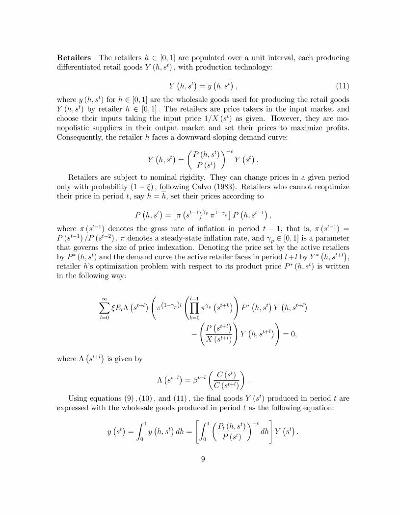
Retailers The retailers h 2 [0; 1] are populated over a unit interval, each producingdi¤erentiated retail goods Y (h; st) ; with production technology:

Y�h; st

�= y

�h; st

�; (11)

where y (h; st) for h 2 [0; 1] are the wholesale goods used for producing the retail goodsY (h; st) by retailer h 2 [0; 1] : The retailers are price takers in the input market andchoose their inputs taking the input price 1=X (st) as given. However, they are mo-nopolistic suppliers in their output market and set their prices to maximize pro�ts.Consequently, the retailer h faces a downward-sloping demand curve:

Y�h; st

�=

�P (h; st)

P (st)

���Y�st�:

Retailers are subject to nominal rigidity. They can change prices in a given periodonly with probability (1� �) ; following Calvo (1983). Retailers who cannot reoptimizetheir price in period t; say h = h; set their prices according to

P�h; st

�=���st�1

� p �1� p�P �h; st�1� ;where � (st�1) denotes the gross rate of in�ation in period t � 1, that is, � (st�1) =P (st�1) =P (st�2) : � denotes a steady-state in�ation rate, and p 2 [0; 1] is a parameterthat governs the size of price indexation. Denoting the price set by the active retailersby P � (h; st) and the demand curve the active retailer faces in period t+ l by Y �

�h; st+l

�,

retailer h�s optimization problem with respect to its product price P � (h; st) is writtenin the following way:

1Xl=0

�Et��st+l� �(1� p)l

l�1Yk=0

� p�st+k

�!P ��h; st

�Y�h; st+l

�� P�st+l�

X (st+l)

!Y�h; st+l

�!= 0;

where ��st+l�is given by

��st+l�= �t+l

�C (st)

C (st+l)

�:

Using equations (9) ; (10) ; and (11) ; the �nal goods Y (st) produced in period t areexpressed with the wholesale goods produced in period t as the following equation:

y�st�=

Z 1

0

y�h; st

�dh =

"Z 1

0

�Pt (h; s

t)

P (st)

���dh

#Y�st�:

9

Moreover, because of stickiness in the retail goods price, the aggregate price indexfor �nal goods P (st) evolves according to the following law of motion:

P�st�1��

= (1� �)P ��h; st

�1��+ �

���st�1

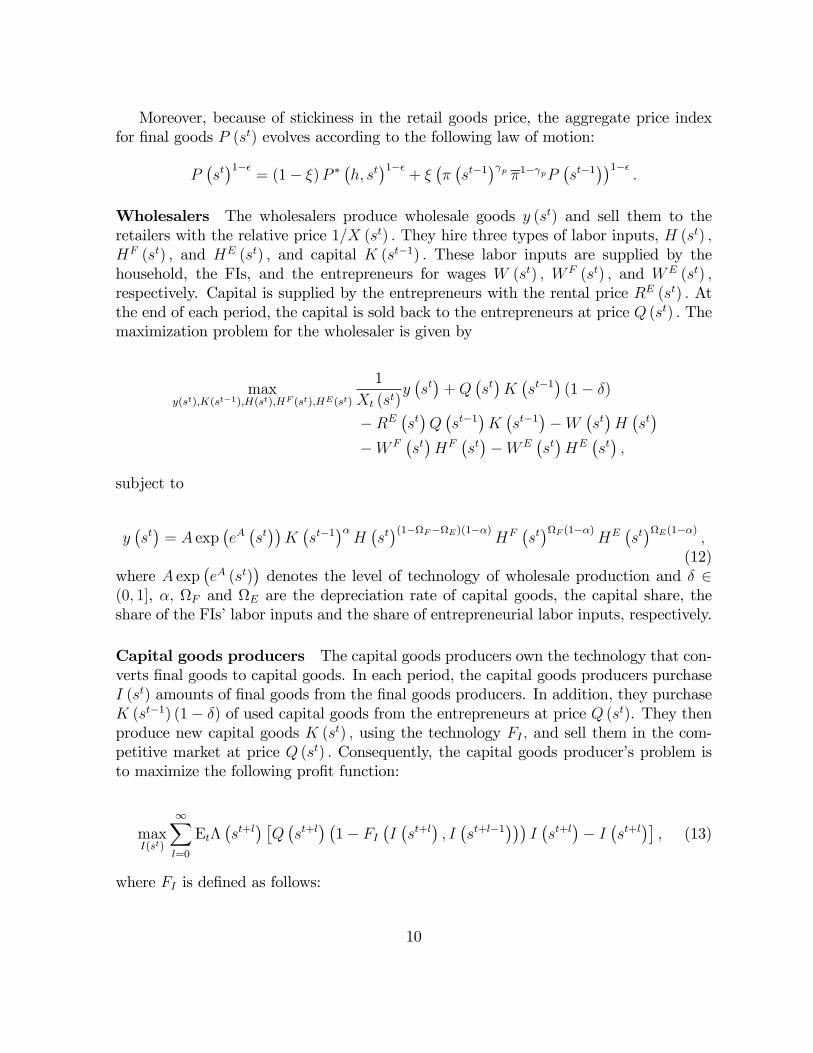
� p �1� pP �st�1��1�� :Wholesalers The wholesalers produce wholesale goods y (st) and sell them to theretailers with the relative price 1=X (st) : They hire three types of labor inputs, H (st) ;HF (st) ; and HE (st) ; and capital K (st�1) : These labor inputs are supplied by thehousehold, the FIs, and the entrepreneurs for wages W (st) ; W F (st) ; and WE (st) ;respectively. Capital is supplied by the entrepreneurs with the rental price RE (st) : Atthe end of each period, the capital is sold back to the entrepreneurs at price Q (st) : Themaximization problem for the wholesaler is given by

maxy(st);K(st�1);H(st);HF (st);HE(st)

1

Xt (st)y�st�+Q

�st�K�st�1

�(1� �)

�RE�st�Q�st�1

�K�st�1

��W

�st�H�st�

�W F�st�HF

�st��WE

�st�HE

�st�;

subject to

y�st�= A exp

�eA�st��K�st�1

��H�st�(1�F�E)(1��)HF

�st�F (1��)HE

�st�E(1��) ;

(12)where A exp

�eA (st)

�denotes the level of technology of wholesale production and � 2

(0; 1], �; F and E are the depreciation rate of capital goods, the capital share, theshare of the FIs�labor inputs and the share of entrepreneurial labor inputs, respectively.

Capital goods producers The capital goods producers own the technology that con-verts �nal goods to capital goods. In each period, the capital goods producers purchaseI (st) amounts of �nal goods from the �nal goods producers. In addition, they purchaseK (st�1) (1� �) of used capital goods from the entrepreneurs at price Q (st). They thenproduce new capital goods K (st) ; using the technology FI ; and sell them in the com-petitive market at price Q (st) : Consequently, the capital goods producer�s problem isto maximize the following pro�t function:

maxI(st)

1Xl=0

Et��st+l� �Q�st+l� �1� FI

�I�st+l�; I�st+l�1

���I�st+l�� I

�st+l��; (13)

where FI is de�ned as follows:

10

FI�I�st+l�; I�st+l�1

��� �

2

exp(eI(st))I

�st+l�

I (st+l�1)� 1!2: (14)

Note that � is a parameter that is associated with investment technology with an ad-justment cost, where eI(st) is the shock to the adjustment cost.6 Here, the developmentof the total capital available at period t is described as

K�st�=�1� FI

�I�st�; I�st�1

���I�st�+ (1� �)K

�st�1

�: (15)

Government The government collects a lump-sum tax from the household T (st) andspends G (st). A budget balance is maintained for each period t: Thus, we have

G�st�exp

�eG(st)

�= T

�st�; (16)

where eG(st) is the stochastic component of government spending.

Monetary authority In our baseline model, the monetary authority sets the nominalinterest rate Rn (st) according to a standard Taylor rule with inertia:

Rn�st�= �Rn

�st�1

�+ (1� �)

���(�

�st�) + �y log

�Y (st)

Y

��+ eR

�st�; (17)

where � is the autoregressive parameter of the policy rate, �� and �y are the policy weight

on the in�ation rate of �nal goods � (st) and the output gap log�Y (st)Y

�; respectively,

and eR(st) is the shock to the monetary policy rule. Because the monetary authoritydetermines the nominal interest rate, the real interest rate in the economy is given bythe following Fisher equation:

R�st�� Et

�Rn (st)

� (st+1)

�: (18)

Resource constraint The resource constraint for �nal goods is written as

Y�st�= C

�st�+ I

�st�+G

�st�exp

�eG(st)

�+ �EGE

�!E�st��RE�st�Q�st�1

�K�st�1

�+ �FGF

�!F�st��RF�st� �Q�st�1

�K�st�1

��NE

�st�1

��+ CF

�st�+ CE

�st�: (19)

6Equation (13) does not include a term for the purchase of the used capital K�st�1

�from the

entrepreneurs at the end of the period. This is because we assume, following BGG (1999), that the priceof old capital that the entrepreneurs sell to the capital goods producers, which we denote as Q (st) ; isclose to the price of the newly produced capital Q (st) around the steady state.

11

Note that the fourth and the �fth terms on the right-hand side of the equation correspondto the monitoring costs incurred by the FIs and investors, respectively. The last two termsare the FIs�and entrepreneurs�consumption.

Law of motion for exogenous variables There are �ve equations for the shockprocesses, eA (st) ; eI (st), eB (st) ; eG (st) ; and eR (st) ; following processes as below:

eA�st�= �Ae

A�st�1

�+ "A

�st�; (20)

eI�st�= �Ie

I�st�1

�+ "I

�st�; (21)

eB�st�= ��e

B�st�1

�+ "�

�st�; (22)

eG�st�= �Ge

G�st�1

�+ "G

�st�; (23)

eR�st�= �Re

R�st�1

�+ "R

�st�; (24)

where �A; �I ; �B; �G; and �R 2 (0; 1) are autoregressive roots of the exogenous variablesand "A (st) ; "I (st) ; "B (st) ; "G (st) ; and "R (st) are innovations that are mutually inde-pendent, serially uncorrelated, and normally distributed with mean zero and variances�2A; �

2I ; �

2�; �

2G; and �

2R, respectively.

2.3 Equilibrium Condition

An equilibrium consists of a set of prices, fP (h; st) for h 2 [0; 1] ; P (st); X(st); R (st) ;RF (st) ; RE (st) ;W (st) ; W F (st) ; WE (st) ; Q (st) ; RF (st+1) ; RE (st+1) ; ZF (st+1) ;ZE (st+1)g1t=0, and the allocations f!F (st+1)g1t=0; f!E (st+1)g1t=0; fNF (st)g1t=0; fNE (st)g1t=0ffy(h; st)); Y (h; st) for h 2 [0; 1] ; Y (st) ; C (st) ; D (st) ; I (st) ; K (st) ; H (st) ; HF (st) ;HE (st)gg1t=0; for a given government policy fRn (st) ; G (st) ; T (st)g1t=0, realization ofexogenous variables f"A (st) ; eB(st); eG(st); eI(st); "R (st) ; "NE

(st) ; "NF(st)g1t=0 and

initial conditions NF�1; N

E�1; K�1 such that for all t and h:

(1) a household maximizes its utility given the prices;(2) the FIs maximize their pro�ts given the prices;(3) the entrepreneurs maximize their pro�ts given the prices;(4) the �nal goods producers maximize their pro�ts given the prices;(5) the retail goods producers maximize their pro�ts given the prices;(6) the wholesale goods producers maximize their pro�ts given the prices;(7) the capital goods producers maximize their pro�ts given the prices;(8) the government budget constraint holds; and(9) markets clear.

12

3 Data and Estimation Strategy

Following Christensen and Dib (2008) and HSU (2011), we set some of the parametersto the values used in the existing studies. These include the quarterly discount factor �;the labor supply elasticity �; the capital share �; the quarterly depreciation rate �; andthe steady-state share of government expenditure in total output G=Y . See Table 1 forthe values of these parameters.In addition, we calibrate six parameters for the credit contracts: the lenders�mon-

itoring cost in the IF contract �F , the lenders�monitoring cost in the FE contract �E;the standard error of the idiosyncratic productivity shock in the FI sector �F , the stan-dard error of the idiosyncratic productivity shock in the entrepreneurial sector �E, thesurvival rate of FIs F ; and the survival rate of entrepreneurs E, so that the followingsix equilibrium conditions are met at the steady state:

(1) the risk spread, RE �R; is 200 basis points annually;

(2) the ratio of net worth held by FIs to the aggregate capital, NF=QK, is 0.1, ahistorical average in the Japanese economy;

(3) the ratio of net worth held by entrepreneurs to the aggregate capital, NE=QK, is0.5, a historical average in the Japanese economy;

(4) the annualized failure rate of FIs is 3%;

(5) the annualized failure rate of entrepreneurs is 3%; and

(6) the ratio of the spread between the FIs� borrowing rate and the entrepreneurialborrowing rate, ZE � ZF ; to the spread between the entrepreneurial borrowingrate and the riskless rate, ZF � R; is 186/32, the value taken from a historicalaverage.

We estimate the rest of parameters of the model using a Bayesian method. Estimatedparameters are the frequency of price adjustment �; the degree of price indexation p, aparameter that controls the capital adjustment cost �; the coe¢ cients of the policy rule�; �� and �y; the autoregressive parameters of the shock process �A; �I ; �B; �G; and �R,the variances of these shocks �2A; �

2I ; �

2B; �

2G; and �

2R; and the variances of the shocks

to net worth �2NF and �2NE: To calculate the posterior distribution and to evaluate the

marginal likelihood of the model, the Metropolis-Hastings algorithm is employed. To dothis, a sample of 200,000 draws was created, neglecting the �rst 100,000 draws.

13

3.1 Data

Our dataset includes seven time series for the Japanese economy: the growth rate of realGDP, the growth rate of real consumption, the growth rate of real investment, the logdi¤erence of the GDP de�ator, the call rate, and the growth rates of real net worth of thebanking sector and the entrepreneurial sector.7 ;8 In estimating the model, we demeanthese variables, assuming that the mean of each variable in the model coincides with thatin the data, following CMR (2008). Following Sugo and Ueda (2008), the variables otherthan the GDP de�ator and the call rate are demeaned with a trend break in 1991Q2.Our dataset covers the period from 1981Q1 to 2013Q4.9 All data series used for

estimation are shown in Figure 1. The shaded areas are recessions which start at thepeak of business cycles and end at the trough. The reference dates are speci�ed by theEconomic and Social Research Institute of the Japanese government.

3.2 Prior Distribution of the Parameters

Table 2 shows the prior distributions of parameters. The adjustment cost parameter forinvestment � is normally distributed with a mean of 4.0 and a standard error of 1.5;the Calvo probability � is beta distributed with a mean of 0.5 and a standard error of0.15; the degree of indexation to past in�ation p is beta distributed with a mean of 0.5and a standard error of 0.2; the policy weight on the lagged policy rate � is normallydistributed with a mean of 0.75 and a standard error of 0.1; the policy weight on in�ation�� is normally distributed with a mean of 1.5 and a standard error of 0.125; and thepolicy weight on the output gap �y is normally distributed with a mean of 0.125 and astandard error of 0.05.The priors on the autoregressive parameters �A; �I ; �B; �G; and �R are beta dis-

tributed with a mean of 0.5 and a standard deviation of 0.2. The variances of theinnovations in exogenous variables �2A; �

2I ; �

2�; �

2G; �

2NF, �2NE ; and �

2R are assumed to

follow an inverse-gamma distribution with a mean of 0.01 and a standard deviation of 2.

7The �rst �ve variables are expressed in per capita terms. The two net worth series are de�ated bythe GDP de�ator.

8The two net worth series are constructed based on the �ow of funds accounts.9While existing studies such as Sugo and Ueda (2008) and Hirose and Kurozumi (2010) estimate their

Dynamic Stochastic General Equilibrium models using only the periods where the nominal interest ratehas been well above zero, our sample includes the periods where it has been close to zero. The reason wetake this approach is that the goal of the current paper is to study the role of �nancial intermediationmalfunction throughout the 1990s and 2000s, which covers the three �nancial crises. We con�rmedthat our parameter estimates and impulse response of key macroeconomic variables to structural shockshardly change when we instead use the sample periods until 1995Q4.

14

4 Estimation Results

In this section, we show the estimated parameter values and distilled structural shocks.In addition, we examine the model-generated time series of credit spreads. While creditspreads play the key role in transmitting the FIs�shocks to the real activities in the model,because of the data limitation, we do not make use of the spread data in estimatingthe model. By comparing the model-generated series with a number of actual �nancialstress indicators, we show how well our model captures the developments of credit marketconditions during the lost decade(s).

4.1 Parameter Estimates

Table 2 reports the estimated values of the structural parameters and the standarddeviations of the shocks. For the investment adjustment cost, we obtain � = 8:67. Thisvalue falls between the estimates of 0.65 (Meier and Muller, 2006) and 32.1 (Ireland,2003) reported in the existing studies for the U.S. economy. Our estimates of the degreeof nominal price rigidity, the frequency of price adjustment and the degree of priceindexation, are � = 0:606 and p = 0:074, respectively. These values, in particular thelatter, are smaller than the �ndings in Meier and Muller (2006). The estimated monetarypolicy rule exhibits an active response to current in�ation �� = 1:48; with inertia of theinterest rate � = 0:845; and a mild reaction to the current output �y = 0:024.Shocks to government expenditure and preference are particularly persistent with

AR(1) coe¢ cients of 0.87 and 0.91, respectively, compared with other shocks. Thestandard deviation of the entrepreneurial net worth shocks is 0.335, being the largestamong the shocks. Comparing these estimates with those for the U.S. data reportedin HSU (2011), the value is larger than that of the United States, which is 0.179. Theestimate of the standard deviation of the FIs�net worth shocks is almost double that ofthe United States, which is 0.041.

4.2 Identi�ed Shocks to Net Worth

We identify time series of seven structural shocks, "A (st) ; eB(st); eG(st); eI(st); "R (st) ;"N

E(st) ; and "N

F(st) ; from 1981Q1 to 2013Q4 based on the estimation. The identi�ed

shocks to the FI�s net worth and the entrepreneurial net worth "NF(st) and "N

E(st) are

displayed in Figure 2a. Similarly to Figure 1, the shaded areas are recessions in Japanesebusiness cycles. Realized values of the two �nancial shocks are negatively related tobusiness cycles: values of the two shocks typically fall below zero during recessions,suggesting that they are contributing to economic downturns. Net worth shocks toentrepreneurs have a large negative value for several years after the asset bubble burstin the early 1990s, during the early 2000s after the dot-com boom ended, and during thelate 2000s when the global �nancial crisis took place. Net worth shocks to the FIs have

15

continuously shown negative values since the asset bubble burst from the early 1990s tothe 2000s.We compare the time series of net worth shocks estimated for Japan�s economy with

those estimated for the U.S. economy. Figure 2b displays identi�ed time series of networth shocks in the United States that are taken from HSU (2011) as well as thosein Japan. Note that in HSU (2011) we estimate the same model as the model in thecurrent paper using time series of the U.S. macroeconomic variables. During the global�nancial crisis, the United States witnessed a large negative net worth shock to bothentrepreneurs and FIs. In contrast, Japan witnessed a large negative net worth shockonly to entrepreneurs and only a moderate negative shock to FIs. This observationdemonstrates that Japanese FIs hardly su¤ered from the global �nancial crisis, thoughthe Japanese economy was severely dampened due to net worth shocks to entrepreneurs.

4.3 Checking the Estimation Results

Following Nolan and Thoenissen (2009), we check the reasonableness of our estimationresults by making use of actual time series of an indicator of external �nance premiumZE � R: Note that since we do not employ an external �nance premium in estimatingmodel parameters and shocks, we can assess the validity of our estimation results bycomparing indicators and the model-generated external �nance premium. As discussedin De Graeve (2008), however, the data series of the external �nance premium thatcorresponds to the model�s external �nance premium is often di¢ cult to observe, andthis is why we did not use the data for estimation. To this end, we compare timeseries data of four indicators of the external �nance premium with the time series of theexternal �nance premium ZE (st)�R (st) generated from our model. The four indicatorsinclude two market spreads: the spread between bank lending rates on contracted short-term loans and short-term government bond rates and the spread between bank lendingrates on newly contracted short-term loans and short-term government bond rates, andtwo di¤usion indices, the Financial Position Di¤usion Index and the Lending Attitudeof Financial Institutions Di¤usion Index. The index series are of the Tankan (Short-Term Economic Survey of Enterprises in Japan) released from the Bank of Japan. Theyindicate the strain that non-�nancial �rms face in raising external funds from �nancialinstitutions.10

Table 3 presents cross-correlation coe¢ cients between those four measures and themodel-generated series ZE (st) � R (st) for a one-year range of leads and lags that arecomputed from the sample period from 1981 to 2013.11 The model-generated series

10The Financial Position Di¤usion Index is constructed from the number of �rms that report �Easy�minus the number of �rms that report �Tight.�The Lending Attitude Di¤usion Index is constructedfrom the number of �rms that report �Accommodative�minus the number of �rms that report �Severe.�11Correlation coe¢ cients regarding the second measure are computed from the data series from 1993

onward because of the data availability of the series.

16

positively correlates with the �rst, third, and forth indicators in a statistically signi�cantmanner, indicating that our estimated model well captures developments in cost that areassociated with external funding or those of demand for funding of non-�nancial �rmsin Japan. Though the model generated series displays a weaker statistical relationshipwith the second indicator, the coe¢ cients are positive in most leads and lags.

5 Financial Factors in Japanese Business Cycles

In this section, we study the role of net worth shocks to the FI and entrepreneurial sectorin generating macroeconomic dynamics in the Japanese economy. We �rst describe theimpacts of net worth shocks on the macroeconomy and discuss how they di¤er from theimpacts of other shocks. We then examine the relative signi�cance of net worth shocksin accounting for variations in key macroeconomic variables.

5.1 Impulse Responses

Figure 3 shows the impulse responses of key macroeconomic variables to shock to FIs�net worth, and entrepreneurial net worth, productivity, and investment adjustment cost"N

F(st), "N

E(st) ; "A (st) ; and "I (st) : We normalize the size of the shocks to be one

standard deviation. We give positive shocks to the investment adjustment cost andnegative shocks to the other three variables.The net worth shocks to the FIs and entrepreneurs are those that arise as innovations

to equations (6) and (7), respectively. At the impact, they in�uence the terms of creditcontracts ZF (st+1) and ZE (st+1) and they are propagated to the rest of the economy bychanging volume of �nancial intermediation. For instance, when the balance sheets of FIsare impaired by a negative net worth shock, investors require a higher expected returnZF (st+1) in their credit contracts with the FIs because the borrower FIs are now lesscreditworthy than otherwise. The increase in the FIs�borrowing rate is translated to theentrepreneurial borrowing rate as shown in the panel (8). With a higher cost of borrowingexternal funds, the entrepreneurs purchase less capital goods K (st) from capital goodsproducers. This results in a lower capital input supply, dampening investment andGDP. In�ation falls, re�ecting the weakened aggregate demand. The decline in demandfor capital goods K (st) causes the second-round e¤ect on the endogenous developmentsin the net worths of FI�s and those of entrepreneurs by a¤ecting the capital goods priceQ (st) : That is, a reduced value of capital goods price, shown in the panel (3), hampersthe net worth accumulation of the two sectors since the retained earnings in the thesesectors decrease following equations (6) and (7). The deteriorated net worths result inthe further rise in borrowing rates, dampening investment and GDP further.In response to a negative shock to productivity in the wholesaler�s production func-

tion (12) ; because less output is produced from the same amount of production inputs,investment and output are reduced. In�ation increases as the real marginal cost of the

17

wholesaler increases. The increase in in�ation leads the central bank to raise the nom-inal interest rate according to the Taylor rule (17), having a contractionary e¤ect onoutput. Similarly to the consequence of net worth shocks, a decline in aggregate invest-ment demand lowers the capital goods price Q (st) : Consequently, as shown in the panels(5) and (6), the �nancial accelerator e¤ect emerges through endogenous deterioration ofnet worth in both the FI and entrepreneurial sectors. Impaired balance sheets in thesesectors reinforce the adverse e¤ects of the productivity shock on the aggregate economy.In response to a positive shock to the investment adjustment cost (14) ; the capital

goods priceQ (st) increases, while the other types of shocks lower it. This is because otherthings being equal capital goods producers need to purchase more �nal goods to producethe same amount of capital goods K (st). Since capital goods become more expensivethan otherwise, capital input supply is reduced, resulting in a lower aggregate investmentand GDP. Although the increase in the capital goods price helps the accumulation ofnet worth in the FI and entrepreneurial sectors as shown in the panels (5) and (6) andreduces the entrepreneurial borrowing rate, this favorable e¤ect is dominated by theadverse e¤ect due to the increase in the capital goods price.

5.2 Historical Decomposition

Using the time series of structural shocks that are extracted from the estimation above,we next evaluate how shocks to the net worth of FIs and entrepreneurs a¤ected macro-economic �uctuations in Japan over the last thirty years. Figure 4 plots historical de-compositions of �uctuations in investment, GDP, and in�ation into structural shocks.This �gure suggests that shocks to the net worth of entrepreneurs have contributed

substantially to the declines in investment during the period of the �rst crisis in the early1990s and during the period of the third crisis in the late 2000s. As illustrated in Figure3, negative entrepreneurial net worth shocks cause �nancial intermediation malfunctionby increasing entrepreneurs�borrowing rates and reducing the amount of funds that areintermediated from households to entrepreneurs, leading to economic downturn. It isseen that the net worth shocks also contributed to a decline in investment during therecession that started from November 2000 as the boom in IT industry ended. The GDPand in�ation rate have been dampened by the shocks as well particularly during the�rst and the third crises. In contrast to �uctuations in investment, �uctuations in thesevariables are more a¤ected by TFP shocks.Compared with entrepreneurial net worth shocks, the e¤ects on �uctuations in in-

vestment of net worth shocks to the FIs have been relatively minor. In particular, thecontribution of these shocks to investment decline during the third crisis was negligible.This observation is consistent with the view that the origin of the current global �nan-cial crisis is the deterioration of the balance sheets of U.S. banks rather than those ofJapanese banks. The FIs�net worth shocks, however, have been continuously dampen-ing investment since the burst of the asset price bubble, and the impact of these shocks

18

has been sizable throughout the 1990s. As documented by Hoshi and Kashyap (2010),Japanese banks have been su¤ering from non-performing loan problems and recordedloan losses of about 13 trillion yen in 1996, 1998, and 1999, and their balance sheetswere severely impaired. Our estimation results show that the impaired balance sheetsof the FIs have dampened �nancial intermediation and reduced loan supply to �rms,which is consistent with the documentation. The adverse e¤ects of the shocks have beengradually diminishing since early 2000. This timing is consistent with the time the Fi-nancial Revival Program was launched by the Japanese Financial Service Agency ledby Heizo Takenaka and when the Japanese government started to increase pressure onlarge Japanese banks to strengthen their capital conditions. The shocks also have beencontributing to lower GDP and in�ation throughout the 1990s.Shocks to the investment adjustment cost have been an important driver of investment

declines during periods other than the three �nancial crisis periods. For instance, duringthe recession that started in June 1985 and during the period of moderate economicslowdown around the mid-2000s, these shocks were the key determinant of �uctuationsin investment.Table 4 computes the average contribution of each shock in accounting for three

macroeconomic variables over the full sample period, the 1990s, and the late 1990s. It isseen that the quantitatively most important shocks in explaining investment �uctuationsare shocks to the investment adjustment cost. The net worth shocks to entrepreneursare the second most important shocks. The contribution to investment �uctuations ofnet worth shocks to the FIs is small for the full sample basis, though it is relatively largefor the late 1990s.

6 Financial Friction and Investment Adjustment Cost

In addition, we explore how the investment adjustment cost shocks are related to thenet worth shocks estimated in our model. As discussed by Justiniano, Primiceri, andTambalotti (2008), the estimates of the New Keynesian model typically indicate thatshocks to investment adjustment cost play an important role in producing business cycles.Christensen and Dib (2008) also report that more than 90% of investment variationsoriginate in the shocks to investment e¢ ciency in the U.S. economy. Hirose and Kurozumi(2010) by estimating a New Keynesian model using Japanese data also document thatmost of the Japanese investment variations are accounted for by these shocks. Theseshocks are considered to be related to the e¢ ciency of �nancial intermediation in Hiroseand Kurozumi (2008) and Justiniano, Primiceri, and Tambalotti (2011).To see how investment adjustment cost shocks are related to �nancial factors, we

estimate models that abstract from �nancial frictions and compare the role of estimatedinvestment adjustment cost shocks in these models with that in the current model.The alternative models are the BGG model and the Non-FA (non-�nancial-accelerator)model. In the BGG model, entrepreneurs are credit constrained but FIs are not. In the

19

Non-FA model, no credit market imperfection prevails in the economy. To illustrate therole that shocks to the FIs�net worth play, we estimate the BGG model and the Non-FAmodel along with the benchmark model by a Bayesian method.Table 5 reports the variance decompositions of investment under the three models.

Under the Non-FA model, a bulk of the variations comes from the shocks to investmentadjustment cost "It , accounting for 94% of the investment variations. When shocksoriginating in the credit market are incorporated, the contribution of the shocks toinvestment adjustment cost decreases. The estimated contribution of "It is 77% and64%, respectively, in the BGG model and the benchmark model. On the other hand,under the two models, a signi�cant portion of investment variation is attributed to thecontributions of shocks originating in the credit market, "N

E

t and "NF

t . The contributionof "N

E

t under the benchmark model is larger than under the BGG model. This is becausethe ampli�cation and propagation mechanism is increased under the benchmark model.

7 Conclusion

In this paper, we have assessed the roles of �nancial shocks in accounting for macroeco-nomic �uctuations in Japan particularly during the periods when �nancial crises havetaken place. To this end, we have borrowed a version of �nancial accelerator modeldeveloped by Hirakata, Sudo, and Ueda (2011). In this model, unexpected shocks to thenet worths of FIs and entrepreneurs a¤ect macroeconomic �uctuations by a¤ecting theterms of credit contracts and external �nance premiums that are relevant to the volumeof aggregate investment. We have estimated the model using Japanese data from the1980s to the 2010s to obtain model parameters and underlying structural shocks. Usingthe estimation results, we have decomposed �uctuations of macroeconomic variables intothose attributed to �nancial shocks and those attributed to non-�nancial shocks.We have found that the two �nancial shocks, shocks to the net worths of FIs and

entrepreneurs, are both important sources of macroeconomic �uctuation. These shocksimpair the balance sheets of the two sectors, increase the external �nance premium, anddampen aggregate investment. Their impacts on investment are prominent particularlyduring the three �nancial crises. Net worth shocks to entrepreneurs have played thekey role in lowering investment during the periods of the bubble burst and the global�nancial crisis. Net worth shocks to FIs have contributed to investment decline in theearly 1990s and persistently lowered investment throughout the 1990s.In addition, our result suggests that the shocks to investment adjustment cost that

are emphasized in the existing studies may be capturing shocks to the �nancial sector.The comparison with other models that abstract from credit-constrained banks, credit-constrained entrepreneurs, or both, illustrates that investment variations explained bythe shocks to capital adjustment cost are reduced drastically by inclusion of the creditmarket imperfection.Finally, let us propose three important directions for future research. The �rst is

20

to incorporate the zero lower bound of nominal interest rates and/or unconventionalmonetary policy. The second direction is to embed the stochastic trend in the currentmodel to explain a kinked decline in GDP growth rates since the burst of the bubble.Third, another model for �nancial shocks is possible. Speci�cally, riskiness shocks ratherthan net worth shocks have attracted attention following the work of Christiano, Motto,and Rostagno (2014).

21

A Credit Contracts

In this appendix, we discuss how the contents of the two credit contracts are determinedby the pro�t maximization problem of the FIs. We �rst explain how the FIs earn pro�tfrom the credit contracts and then explain the participation constraints of the otherparticipants in the credit contracts.In each period t; the expected net pro�t of an FI from the credit contracts is expressed

by:

Xst+1

��st+1

� share of FIs earnings received by FIz }| {�1� �F

�!F�st+1

���RF�st+1

� �Qt�st�K�st��NE

�st��; (25)

where �(st+1) is a probability weight for state st+1: Here, the expected return on theloans to entrepreneurs, RF (st+1) is given by:

share of entrepreneurial earnings received by FIz }| {��E�!E�st+1

��� �EGE

�!E�st+1

���RE�st+1

�Q�st�K�st�

� RF�st+1

� �Q�st�K�st��NE

�st��for 8st+1: (26)

This equation indicates that the two credit contracts determine the FIs�pro�ts. In theFE contract, the FIs receive a portion of what entrepreneurs earn from their projects astheir gross pro�t. In the IF contract, the FIs receive a portion of what they receive fromthe FE contract as their net pro�t and pay the rest to investors.There is a participation constraint in each of the credit contracts. In the FE contract,

the entrepreneurs�expected return is set to equal the return from their alternative option.We assume that without participating in the FE contract, entrepreneurs can purchasecapital goods with their own net worth NE (st) : Note that the expected return fromthis option equals RE (st+1)NE (st). Therefore the FE contract is agreed upon theentrepreneurs only when the following inequality is expected to hold:

share of entrepreneurial earnings kept by the entrepreneurz }| {�1� �E

�!E�st+1

���RE�st+1

�Q�st�K�st�

� RE�st+1

�NE

�st�for 8st+1: (27)

We next consider a participation constraint of the investors in the IF contract. Weassume that there is a risk-free rate of return in the economy R (st) and that investors

22

may alternatively invest in this asset. Consequently, for investors to join the IF contract,the loans to the FIs must equal the opportunity cost of lending. That is:

share of FIs�earnings received by the investorsz }| {��F�!F�st+1

��� �FGF

�!F�st+1

���RF�st+1

� �Q�st�K�st��NE

�st��

� R�st� �Q�st�K�st��NF

�st��NE

�st��: (28)

The FI maximizes its expected pro�t (25) by optimally choosing the variables !F (st+1) ;!E (st+1) ; and K (st) ; subject to the entrepreneurial participation constraint (27) andthe investors�participation constraint (28). Combining the �rst-order conditions yieldsthe following equation:

0 =Xst+1

��st+1

� ��1� �F

�!F�st+1

����E�st+1

�RE�st+1

�+�0F�!F (st+1)

��0F (st+1)

�F�st+1

��E�st+1

�REt+1

�st+1

���0F�!F (st+1)

��0F (st+1)

R(st)

+

�1� �F

�!F (st+1)

��0E (st+1)

�0E�!E (st+1)

� �1� �E

�!E�st+1

���RE�st+1

�+�0F�!F (st+1)

��F (st+1) �0E (st+1)

�0F (st+1) �0E�!E (st+1)

� �1� �E

�!E�st+1

���RE�st+1

�): (29)

Using equations (26) and (28), we obtain equation (1) in the text.

23

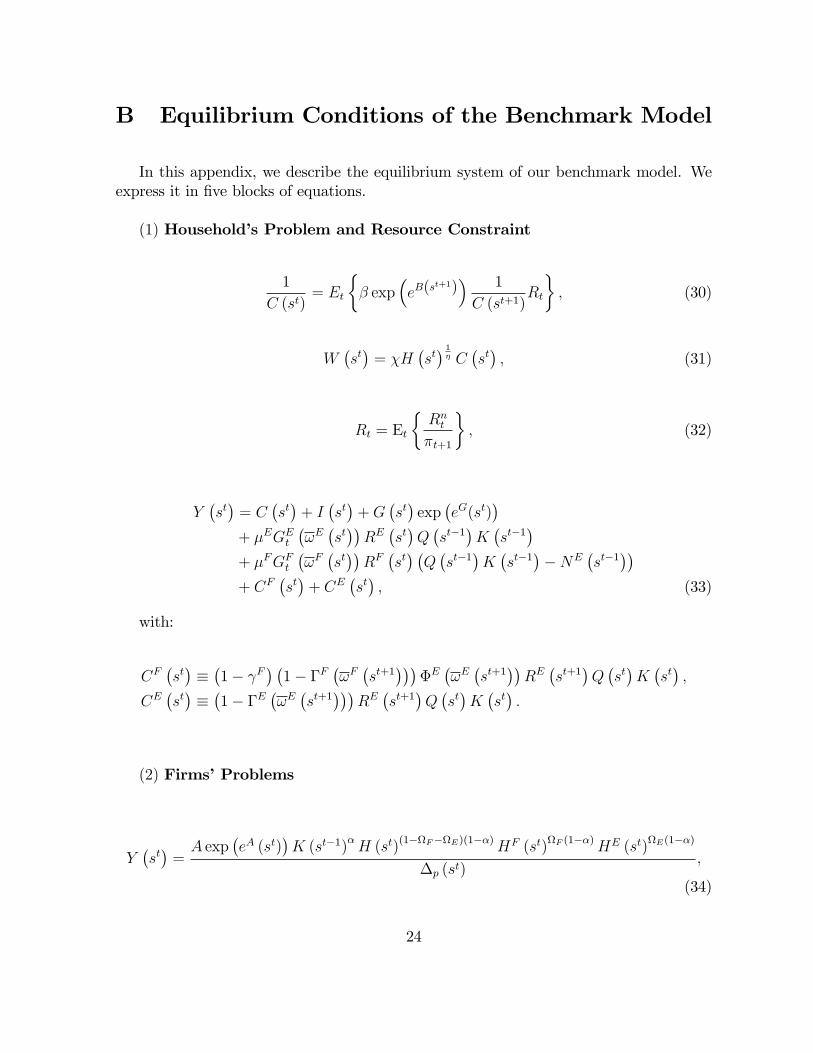
B Equilibrium Conditions of the Benchmark Model

In this appendix, we describe the equilibrium system of our benchmark model. Weexpress it in �ve blocks of equations.

(1) Household�s Problem and Resource Constraint

1

C (st)= Et

�� exp

�eB(s

t+1)� 1

C (st+1)Rt

�; (30)

W�st�= �H

�st� 1� C

�st�; (31)

Rt = Et

�Rnt�t+1

�; (32)

Y�st�= C

�st�+ I

�st�+G

�st�exp

�eG(st)

�+ �EGEt

�!E�st��RE�st�Q�st�1

�K�st�1

�+ �FGFt

�!F�st��RF�st� �Q�st�1

�K�st�1

��NE

�st�1

��+ CF

�st�+ CE

�st�; (33)

with:

CF�st���1� F

� �1� �F

�!F�st+1

����E�!E�st+1

��RE�st+1

�Q�st�K�st�;

CE�st���1� �E

�!E�st+1

���RE�st+1

�Q�st�K�st�:

(2) Firms�Problems

Y�st�=A exp

�eA (st)

�K (st�1)

�H (st)

(1�F�E)(1��)HF (st)F (1��)HE (st)

E(1��)

�p (st);

(34)

24

with:

�p

�st�= (1� �)

�Kp (s

t)

Fp (st)

���+ �

�� (st�1)

p

� (st)

����p

�st�1

�;

Fp�st�= 1 + �� exp

�eB(s

t+1)� C (st)Y (st+1)C (st+1)Y (st)

�� (st)

p

� (st+1)

�1��Fp�st+1

�;

Kp

�st�=

� (st)

� (st)� 1MC�st�+ �� exp

�eB(s

t+1)� C (st)Y (st+1)C (st+1)Y (st)

�� (st)

p

� (st+1)

���Kp

�st+1

�;

H�st�W�st�= A exp

�eA�st��K�st�1

��H�st�(1�F�E)(1��)HF

�st�F (1��)HE

�st�E(1��)

�MC�st�(1� �) (1� F � E) ; (35)

RE�st�=�Y (st) =K (st) +Q (st+1) (1� �)

Q (st); (36)

Q�st� 1� 0:5�

�I (st) exp(eI(st))

I (st�1)� 1�2!

�Q�st���

�I (st) exp(eI(st))

I (st�1)

��I (st) exp(eI(st))

I (st�1)� 1��

� 1

= Et

(� exp

�eB(s

t+1)� C (st)Q (st+1)

C (st+1)�

�I (st+1) exp(eI(st+1))

I (st)

�2�I (st+1)

I (st)� 1�exp(eI(st+1))

):

(37)

(3) FIs�Problems

Equilibrium conditions for credit contracts are given by (27), (28), and (29) and bythe following equations:

GF�!F�st��=

1p2�

Z log!F (st)�0:5�2F�F

�1exp

��v

2F

2

�dvF ; (38)

25

GE�!E�st��=

1p2�

Z log!E(st)�0:5�2E�E

�1exp

��v

2E

2

�dvE; (39)

G0F�!F (st)

�� @GF (!F (st))

@!F (st)

=�

1p2�

��1

!F (st)�F

�exp

�:5

�log!F (st)�0:5�2F

�F

�2!;

(40)

G0E�!E (st)

�� @GE(!E(st))

@!E(st)

=�

1p2�

��1

!E(st)�E

�exp

�:5

�log!E(st)�0:5�2E

�E

�2!;

(41)

�F�!F (st)

�= 1p

2�

R log!F (st)�0:5�2F�F

�1 exp��v2F

2

�dvF

+!F (st)p

2�

R1log!F (st)+0:5�2F

�F

exp��v2F

2

�dvF ;

(42)

�E�!Et�= 1p

2�

R log!E(st)�0:5�2E�E

�1 exp��x2

2

�dvE

+!E(st)p

2�

R1log!E(st)+0:5�2E

�E

exp��v2E

2

�dvE;

(43)

�0F�!F�st���@�F

�!F (st)

�@!F (st)

=1p

2�!F (st)�Fexp

�:5

�log!F (st)� 0:5�2F

�F

�2!

+1p2�

Z 1

log!F (st)+0:5�2F�F

exp

��v

2F

2

�dvF �

1p2��F

exp

0BBB@��log!F (st)+0:5�2F

�F

�22

1CCCA ;(44)

26

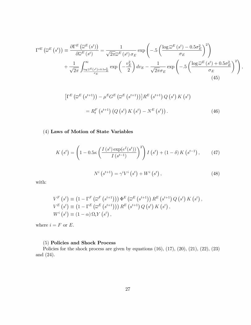
�0E�!E�st���@�E

�!E (st)

�@!E (st)

=1p

2�!E (st)�Eexp

�:5

�log!E (st)� 0:5�2E

�E

�2!

+1p2�

Z 1

log!E(st)+0:5�2E�E

exp

��v

2E

2

�dvE �

1p2��E

exp

�:5

�log!E (st) + 0:5�2E

�E

�2!;

(45)

��E�!E�st+1

��� �EGE

�!E�st+1

���RE�st+1

�Q�st�K�st�

= RFt�st+1

� �Q�st�K�st��NE

�st��: (46)

(4) Laws of Motion of State Variables

K�st�=

1� 0:5�

�I (st) exp(eI(st))

I (st�1)

�2!I�st�+ (1� �)K

�st�1

�; (47)

N i�st+1

�= iV i

�st�+W i

�st�; (48)

with:

V F�st���1� �F

�!F�st+1

����E�!E�st+1

��RE�st+1

�Q�st�K�st�;

V E�st���1� �E

�!E�st+1

���RE�st+1

�Q�st�K�st�;

W i�st�� (1� �) iY

�st�;

where i = F or E.

(5) Policies and Shock ProcessPolicies for the shock process are given by equations (16), (17), (20), (21), (22), (23)

and (24).

27

C Equilibrium Conditions of Alternative Models

In addition to the benchmark model, we consider two alternative models for comparativeconvenience. The �rst is the Non-FA model, in which no �nancial accelerator mechanismis incorporated. The equilibrium conditions under this model are given by equations (16),(17), (20), (21), (22), (23), (24), (30), (31), (32), (34), (35), (36), (37), and (47), andby the following equations instead of equations (33) and (36), respectively, under thebenchmark model, :

Y�st�= C

�st�+ I

�st�+G

�st�exp

�eG(st)

�; (49)

R�st�= Et

�Y (st) =K (st) +Q (st+1) (1� �)Q (st)

: (50)

The second model is the BGG model in which only entrepreneurs are credit con-strained. The equilibrium conditions in this model are given by equations (7), (16), (17),(20), (21), (22), (23), (24), (30), (31), (32), (34), (35), (36), (37), (39), (41), (43), (45)and (47), and by the following three equations instead of equations (29), (33), and (36),respectively, under the benchmark model:

0 =Xst+1

��st+1

� �1� �E

�!E�st+1

���RE�st+1

�+�0E�!F (st+1)

��0E (st+1)

�E�st+1

�RE�st+1

���0E�!E (st+1)

��0E (st+1)

�E�st+1

�R(st); (51)

Y�st�= C

�st�+ I

�st�+G

�st�exp

�eG(st)

�+ �EGE

�!E�st��RE�st�Q�st�1

�K�st�1

�+ CE

�st�; (52)

with:

CE�st���1� �E

�!E�st+1

���RE�st+1

�Q�st�K�st�;

��E�!E�st+1

��� �EGE

�!E�st+1

���RE�st+1

�Q�st�K�st�

= R�st� �Q�st�K�st��NE

�st��: (53)

28

References

[1] Aikman, D. and M. Paustian (2006). �Bank Capital, Asset Prices and MonetaryPolicy,�Bank of England Working Papers 305, Bank of England.

[2] Baba, N., S. Nishioka, N. Oda, M. Shirakawa, K. Ueda, and H. Ugai (2005). �Japan�sDe�ation, Problems in the Financial System and Monetary Policy,�Monetary andEconomic Studies, Bank of Japan.

[3] Bayoumi, T. (1999). �The Morning After: Explaining the Slowdown in JapaneseGrowth in the 1990s,�Journal of International Economics, 53, 241�59.

[4] Bernanke, B. S., M. Gertler and S. Gilchrist (1999). �The Financial Accelerator ina Quantitative Business Cycle Framework,�in Handbook of Macroeconomics, J. B.Taylor and M. Woodford (eds.), Vol. 1, chapter 21, 1341�1393.

[5] Braun, R. A., and E. Shioji. (2007). �Investment Speci�c Technological Changes inJapan,�Seoul Journal of Economics, 20, 165�199.

[6] Caballero, R., T. Hoshi, and A. Kashyap (2008). �Zombie Lending and DepressedRestructuring in Japan.�American Economic Review, 98, 1943�1977.

[7] Calomiris, C. W., and J. R. Mason (2003). �Consequences of Bank Distress duringthe Great Depression,�American Economic Review, 93, 937�947.

[8] Calvo, G.A. (1983). �Staggered Prices in a Utility-maximizing Framework,�Journalof Monetary Economics, 12, 383�398.

[9] Chen, N. K. (2001). �Bank NetWorth, Asset Prices and Economic Activity,�Journalof Monetary Economics, 48, 415�436.

[10] Christensen, I. and A. Dib (2008). �The Financial Accelerator in an Estimated NewKeynesian Model.�Review of Economic Dynamics, 11, 155�178.

[11] Christiano, L., R. Motto, and M. Rostagno (2003). �The Great Depression andthe Friedman�Schwartz Hypothesis,� Journal of Money, Credit and Banking, 35,1119�1198.

[12] Christiano, L., R. Motto, and M. Rostagno (2008). �Shocks, Structures or MonetaryPolicies? The Euro Area and US after 2001,�Journal of Economic Dynamics andControl, 32, 2476�2506.

[13] Christiano, L., R. Motto, and M. Rostagno (2012). �Risk Shocks,�American Eco-nomic Review, 104, 27�65.

29

[14] De Graeve, F. (2008). �The External Finance Premium and the Macroeconomy: USPost-WWII Evidence,�Journal of Economic Dynamics and Control, 32, 3415�3440.

[15] Fukao, M. (2003). �Financial Sector Pro�tability and Double Gearing,� in Struc-tural Impediments to Growth in Japan, Magnus Blomstrom, Jenny Corbett, FumioHayashi, and Anil Kashyap (eds.), Chicago: University of Chicago Press.

[16] Gilchrist, S. and J. V. Leahy (2002). �Monetary Policy and Asset Prices,�Journalof Monetary Economics, 49, 75�97.

[17] Hayashi F., and E. C. Prescott (2002). �The 1990s in Japan: A Lost Decade,�Review of Economic Dynamics, 5, 206�235.

[18] Hirakata, N., N. Sudo, and K. Ueda (2011). �Do Banking Shocks Matter for theU.S. Economy?�Journal of Economic Dynamics and Control, 35, 2042�2063.

[19] Hirose Y. and T. Kurozumi (2012). �Do Investment-Speci�c Technological ChangesMatter for Business Fluctuations? Evidence from Japan,�Paci�c Economic Review,17, 208�230.

[20] Holmstrom, B., and J. Tirole (1997). �Financial Intermediation, Loanable Funds,and the Real Sector,�Quarterly Journal of Economics, 112, 663�691.

[21] Hoshi, T., and A. K. Kashyap (2004). �Japan�s Financial Crisis and EconomicStagnation�Journal of Economic Perspectives, 18, 3�26.

[22] Hoshi, T. and A. K. Kashyap (2010). �Will the U.S. Bank Recapitalization Succeed?Eight lessons from Japan�Journal of Financial Economics, 97, 398�417.

[23] Hoshi, T., A. K. Kashyap and D. Scharfstein (1991). �Corporate Structure, Liquidityand Investment: Evidence from Japanese Industrial Groups,�Quarterly Journal ofEconomics, 106, 33�60.

[24] Jermann U. and V. Quadrini (2009). �Macroeconomic E¤ects of Financial Shocks,�NBER Working Papers 15338, National Bureau of Economic Research, Inc.

[25] Justiniano, A., G. Primiceri, and A. Tambalotti (2008). �Investment Shocks andBusiness Cycles,�Journal of Monetary Economics, 57, 132�145.

[26] Justiniano, A., G. Primiceri, and A. Tambalotti (2011). �Investment Shocks andthe Relative Price of Investment,�Review of Economic Dynamics, 14, 101�121.

[27] Kashyap, A. K. (2002). �Sorting Out Japan�s Financial Crisis,� Federal ReserveBank of Chicago Economic Perspectives, 4th Quarter 2002, 42�55.

30

[28] Kaihatsu, S., and T. Kurozumi (2014). �Sources of Business Fluctuations: Financialor Technology Shocks?,�Review of Economic Dynamics, 17, 224�242.

[29] Kwon, E. (1998), �Monetary Policy, Land Prices, and Collateral E¤ects on Eco-nomic Fluctuations: Evidence from Japan,�Joural of Japanese and InternationalEconomies, 12, 175�203.

[30] Meh, C. A., and K. Moran (2010). �The Role of Bank Capital in the Propagationof Shocks,�Journal of Economic Dynamics and Control, 34, 555�576.

[31] Meier, A., and G. J. Muller (2006). �Fleshing Out the Monetary Transmission Mech-anism: Output Composition and the Role of Financial Frictions.�Journal of Money,Credit, Banking, 38, 1999�2133.

[32] Nolan, C., and C. Thoenissen (2009). �Financial Shocks and the US BusinessCycle,�Journal of Monetary Economics, 56, 596�604.

[33] Smets, F., and R. Wouters (2005). �Shocks and Frictions in US Business Cycles: ABayesian DSGE Approach,�American Economic Review, 90, 586�606.

[34] Sugo, T. and K. Ueda (2008). �Estimating a Dynamic Stochastic General Equilib-rium Model for Japan,�Journal of the Japanese and International Economies, 22,476�502.

31

(1) Parameters

Parameter Value Description

β .99 Discount Factor

δ .025 Depreciation Rate

α .35 Capital Share

R .99-1

Risk Free Rate

ε 6 Degree of Substitutability

η 3 Elasticity of Labor

χ .3 Utility Weight on Leisure

GY-1

.2 Share of Governement Expenditure at Steady State

(2) Calibrated Parameters

Parameter Value Description

σ E 0.269755 S.E. of Entrepreneurial Idiosyncratic Productivity at Steady State

σ F 0.091600 S.E. of FIs' Idiosyncratic Productivity at Steady State

μ E 0.015812 Bankruptcy Cost Associated with Entrepreneurs

μ F 0.078367 Bankruptcy Cost Associated with FIs

γE

0.983840 Survival Rate of Entrepreneurs

γF

0.962437 Survival Rate of FIs

(3) Steady State Conditions

Description

Risk free rate is the inverse of the subjective discount factor.

Premium for entrepreneurial borrowing rate is .0186/4.

Premium for FIs' borrowing rate is .0032/4.

Default probability in the FE contract is .03/4.

Default probability in the IF contract is .03/4.

Entrepreneurial net worth/capital ratio is set to .5.

FIs' net worth/capital ratio is set to .1

F (ω F)=.03/4

nE

=.5

nF

=.1

Table1: Parameters

Condition

R =.99-1

ZE

=ZF

+.0186/4

ZF

=R +.0032/4

F (ω E)=.03/4

Distr. Mean S.D. Mean10th

percentiles

90th

percentiles

ξ p Beta 0.5 0.15 0.6064 0.5536 0.6588

κ Normal 4 1.5 8.6739 6.6539 10.5424

γ p Beta 0.5 1.5 0.0739 0.0080 0.1386

θ Beta 0.75 0.1 0.8447 0.8193 0.8706

φ π Normal 1.5 0.125 1.4832 1.3486 1.6277

φ y Gamma 0.125 0.5 0.0238 0.0104 0.0364

ρ B Beta 0.5 0.2 0.9145 0.8899 0.9371

ρ I Beta 0.5 0.2 0.3770 0.2444 0.5039

ρ A Beta 0.5 0.2 0.8719 0.8258 0.9210

ρ G Beta 0.5 0.2 0.8045 0.7303 0.8744

ρ R Beta 0.5 0.2 0.0590 0.0108 0.1057

ρ P Beta 0.5 0.2 0.6800 0.5268 0.8257

σ E Normal 0.27 0.01 0.2655 0.2493 0.2817

σ B Normal 0.092 0.005 0.0762 0.0700 0.0829

μ E Normal 0.016 0.002 0.0146 0.0116 0.0181

μ B Normal 0.078 0.01 0.0620 0.0434 0.0804

γF

Beta 0.984 0.01 0.9843 0.9708 0.9984

γB

Beta 0.962 0.01 0.9621 0.9459 0.9780

σ (ε B ) Inv. Gamma 0.01 Inf 0.0019 0.0015 0.0023

σ (ε I ) Inv. Gamma 0.01 Inf 0.0256 0.0211 0.0299

σ (ε G ) Inv. Gamma 0.01 Inf 0.0080 0.0072 0.0088

σ (ε A ) Inv. Gamma 0.01 Inf 0.0111 0.0100 0.0123

σ (ε R ) Inv. Gamma 0.01 Inf 0.0015 0.0013 0.0017

σ (ε NF ) Inv. Gamma 0.01 Inf 0.0814 0.0702 0.0911

σ (ε NE ) Inv. Gamma 0.01 Inf 0.3736 0.3351 0.4137

σ (ε P ) Inv. Gamma 0.01 Inf 0.0896 0.0677 0.1114

Table2: Parameter estimates

Prior distribution Posterior distribution

Spread of interest

rate on contracted

short-term loan rate

Spread of interest

rate on new short-

term loan rate

DI for

financial position

DI for

lending attitude

of FIs

ZE

(+4)-R(+4) 0.463 0.244 0.422 0.587

ZE

(+3)-R(+3) 0.502 0.230 0.469 0.604

ZE

(+2)-R(+2) 0.532 0.209 0.523 0.636

ZE

(+1)-R(+1) 0.544 0.163 0.575 0.667

ZE

(0)-R(0) 0.559 0.091 0.626 0.689

ZE

(-1)-R(-1) 0.571 0.039 0.673 0.697

ZE

(-2)-R(-2) 0.579 0.022 0.715 0.693

ZE

(-3)-R(-3) 0.576 -0.012 0.724 0.667

ZE

(-4)-R(-4) 0.568 -0.042 0.689 0.609

Table3: Correlation with alternative indicators

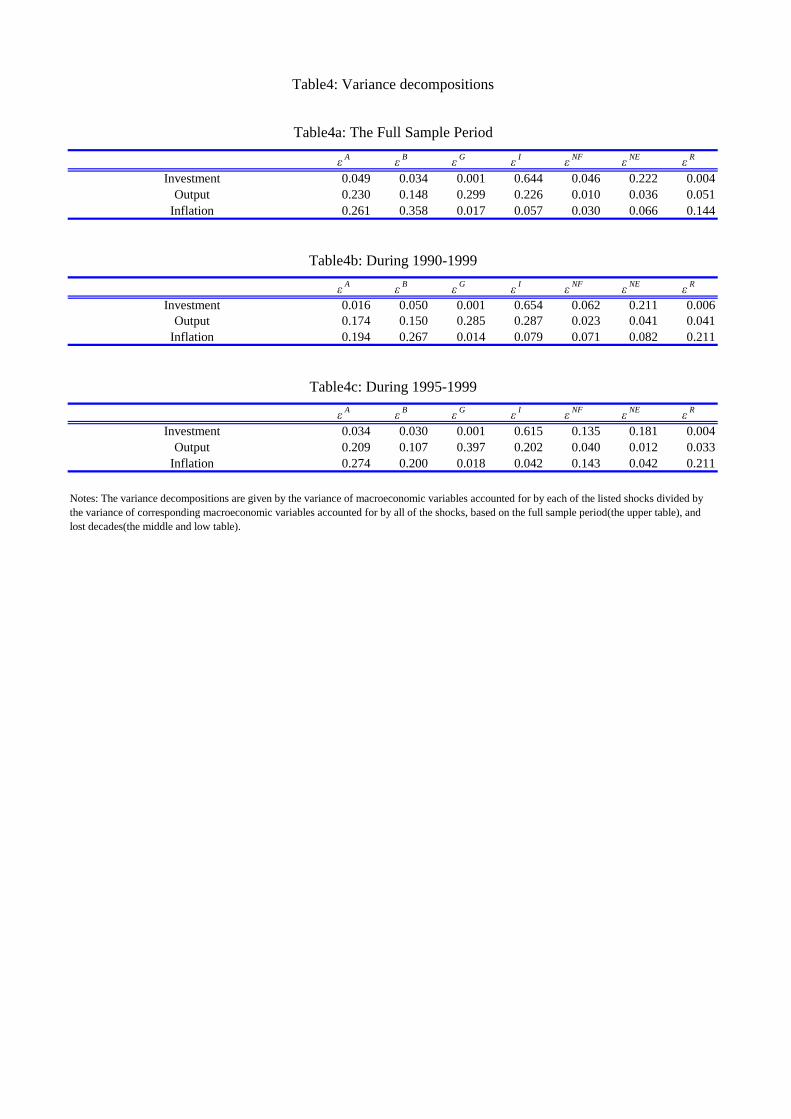
εA

εB

εG

εI

εNF

εNE

εR

Investment 0.049 0.034 0.001 0.644 0.046 0.222 0.004

Output 0.230 0.148 0.299 0.226 0.010 0.036 0.051

Inflation 0.261 0.358 0.017 0.057 0.030 0.066 0.144

εA

εB

εG

εI

εNF

εNE

εR

Investment 0.016 0.050 0.001 0.654 0.062 0.211 0.006

Output 0.174 0.150 0.285 0.287 0.023 0.041 0.041

Inflation 0.194 0.267 0.014 0.079 0.071 0.082 0.211

εA

εB

εG

εI

εNF

εNE

εR

Investment 0.034 0.030 0.001 0.615 0.135 0.181 0.004

Output 0.209 0.107 0.397 0.202 0.040 0.012 0.033

Inflation 0.274 0.200 0.018 0.042 0.143 0.042 0.211

Table4: Variance decompositions

Table4a: The Full Sample Period

Table4b: During 1990-1999

Table4c: During 1995-1999

Notes: The variance decompositions are given by the variance of macroeconomic variables accounted for by each of the listed shocks divided by

the variance of corresponding macroeconomic variables accounted for by all of the shocks, based on the full sample period(the upper table), and

lost decades(the middle and low table).

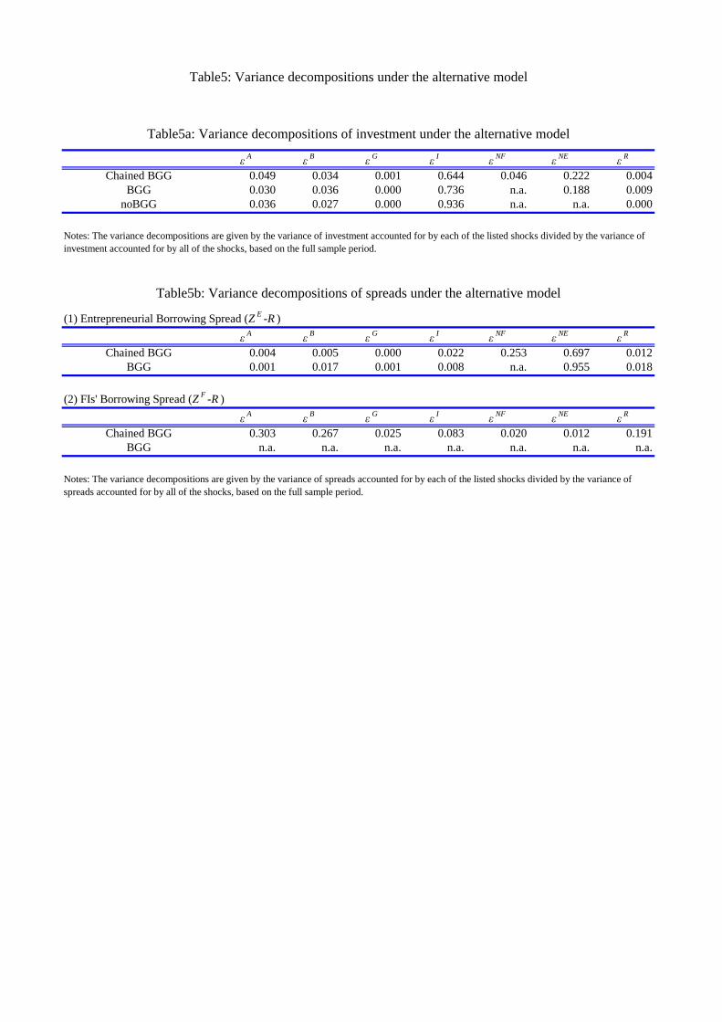
εA

εB

εG

εI

εNF

εNE

εR

Chained BGG 0.049 0.034 0.001 0.644 0.046 0.222 0.004

BGG 0.030 0.036 0.000 0.736 n.a. 0.188 0.009

noBGG 0.036 0.027 0.000 0.936 n.a. n.a. 0.000

(1) Entrepreneurial Borrowing Spread (ZE

-R )

εA

εB

εG

εI

εNF

εNE

εR

Chained BGG 0.004 0.005 0.000 0.022 0.253 0.697 0.012

BGG 0.001 0.017 0.001 0.008 n.a. 0.955 0.018

(2) FIs' Borrowing Spread (ZF

-R )

εA

εB

εG

εI

εNF

εNE

εR

Chained BGG 0.303 0.267 0.025 0.083 0.020 0.012 0.191

BGG n.a. n.a. n.a. n.a. n.a. n.a. n.a.

Table5: Variance decompositions under the alternative model

Table5a: Variance decompositions of investment under the alternative model

Notes: The variance decompositions are given by the variance of investment accounted for by each of the listed shocks divided by the variance of

investment accounted for by all of the shocks, based on the full sample period.

Table5b: Variance decompositions of spreads under the alternative model

Notes: The variance decompositions are given by the variance of spreads accounted for by each of the listed shocks divided by the variance of

spreads accounted for by all of the shocks, based on the full sample period.

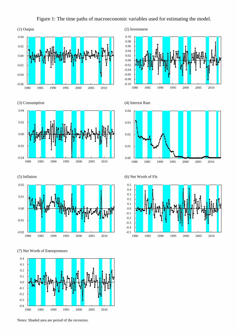
Figure 1: The time paths of macroeconomic variables used for estimating the model.

(1) Output (2) Investment

(3) Consumption (4) Interest Rate

(5) Inflation (6) Net Worth of FIs

(7) Net Worth of Entrepreneurs

Notes: Shaded area are period of the recession.

-0.06

-0.04

-0.02

0.00

0.02

0.04

1980 1985 1990 1995 2000 2005 2010

-0.10

-0.08

-0.06

-0.04

-0.02

0.00

0.02

0.04

0.06

0.08

0.10

1980 1985 1990 1995 2000 2005 2010

-0.04

-0.02

0.00

0.02

0.04

1980 1985 1990 1995 2000 2005 20100.00

0.01

0.02

0.03

0.04

1980 1985 1990 1995 2000 2005 2010

-0.02

-0.01

0.00

0.01

0.02

1980 1985 1990 1995 2000 2005 2010

-0.5

-0.4

-0.3

-0.2

-0.1

0.0

0.1

0.2

0.3

0.4

0.5

1980 1985 1990 1995 2000 2005 2010

-0.4

-0.3

-0.2

-0.1

0.0

0.1

0.2

0.3

0.4

1980 1985 1990 1995 2000 2005 2010

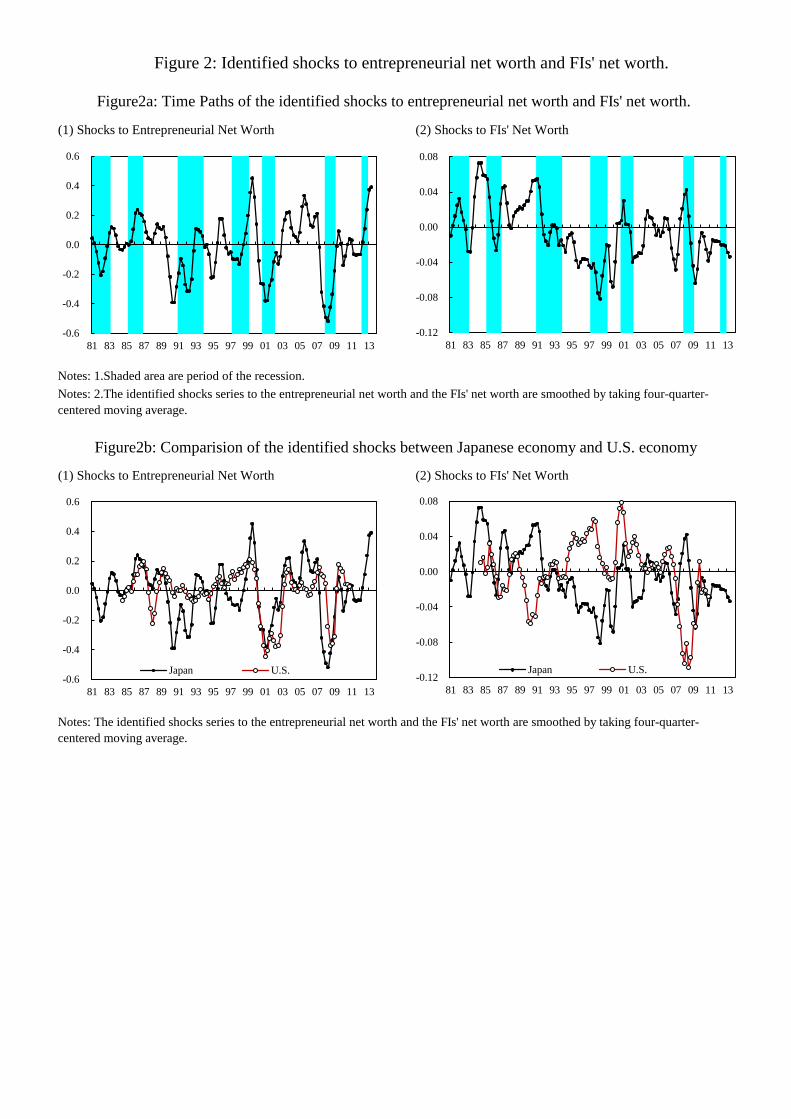
Figure 2: Identified shocks to entrepreneurial net worth and FIs' net worth.

(1) Shocks to Entrepreneurial Net Worth (2) Shocks to FIs' Net Worth

Notes: 1.Shaded area are period of the recession.

(1) Shocks to Entrepreneurial Net Worth (2) Shocks to FIs' Net Worth

Figure2a: Time Paths of the identified shocks to entrepreneurial net worth and FIs' net worth.

Notes: 2.The identified shocks series to the entrepreneurial net worth and the FIs' net worth are smoothed by taking four-quarter-

centered moving average.

Figure2b: Comparision of the identified shocks between Japanese economy and U.S. economy

Notes: The identified shocks series to the entrepreneurial net worth and the FIs' net worth are smoothed by taking four-quarter-

centered moving average.

-0.6

-0.4

-0.2

0.0

0.2

0.4

0.6

81 83 85 87 89 91 93 95 97 99 01 03 05 07 09 11 13

-0.12

-0.08

-0.04

0.00

0.04

0.08

81 83 85 87 89 91 93 95 97 99 01 03 05 07 09 11 13

-0.6

-0.4

-0.2

0.0

0.2

0.4

0.6

81 83 85 87 89 91 93 95 97 99 01 03 05 07 09 11 13

Japan U.S.-0.12

-0.08

-0.04

0.00

0.04

0.08

81 83 85 87 89 91 93 95 97 99 01 03 05 07 09 11 13

Japan U.S.

(1) Investment (2) Output

(3) Tobin's Q (4) Inflation

(5) Net Worth of FIs (6) Net Worth of Entrepreneurs

(7) Nominal Interest Rate (8) Entrepreneurial Borrowing Rate

Figure 3: Impluse responses of the macroeconomic variables to the unexpected impairment of FIs'

networth and entrepreneurial net worth, the unexpected increase in investment adjustment cost, and

the unexpected decline of technology level.

-8

-6

-4

-2

0

2

0 2 4 6 8 10 12 14 16 18 20

FI's Net Worth Shock Entrepreneurial Net Worth Shock Investment Adjustment Cost Shock TFP shock

10-3

Quarter

-8

-6

-4

-2

0

2

0 2 4 6 8 10 12 14 16 18 20

10-3

Quarter

-15

-10

-5

0

5

10

0 2 4 6 8 10 12 14 16 18 20

FI's Net Worth Shock Entrepreneurial Net Worth Shock Investment Adjustment Cost Shock TFP shock

10-3

Quarter

-2

-1

0

1

2

3

4

0 2 4 6 8 10 12 14 16 18 20

10-3

Quarter

-100

-80

-60

-40

-20

0

20

40

0 2 4 6 8 10 12 14 16 18 20

FI's Net Worth Shock Entrepreneurial Net Worth Shock Investment Adjustment Cost Shock TFP shock

10-3

Quarter

-300

-250

-200

-150

-100

-50

0

50

0 2 4 6 8 10 12 14 16 18 20

10-3

Quarter

-1

0

1

2

0 2 4 6 8 10 12 14 16 18 20

FI's Net Worth Shock Entrepreneurial Net Worth Shock Investment Adjustment Cost Shock TFP shock

10-3

Quarter

-2

0

2

4

0 2 4 6 8 10 12 14 16 18 20

10-3

Quarter

(1) Investment

(2) Output

(3) Inflation

Figure 4: Historial contribution of each structural shocks in investment variations, output variations,

and inflation variations.

-0.3

-0.2

-0.1

0.0

0.1

0.2

0.3

82 83 84 85 86 87 88 89 90 91 92 93 94 95 96 97 98 99 00 01 02 03 04 05 06 07 08 09 10 11 12 13

Monetrary Policy Others Investment Adjustment Cost

TFP Entrepreneurial Net Worth FI's Net Worth

-0.12

-0.10

-0.08

-0.06

-0.04

-0.02

0.00

0.02

0.04

0.06

0.08

82 83 84 85 86 87 88 89 90 91 92 93 94 95 96 97 98 99 00 01 02 03 04 05 06 07 08 09 10 11 12 13

Monetrary Policy Others

Investment Adjustment Cost TFP

Entrepreneurial Net Worth FI's Net Worth

total

-0.08

-0.06

-0.04

-0.02

0.00

0.02

0.04

0.06

0.08

82 83 84 85 86 87 88 89 90 91 92 93 94 95 96 97 98 99 00 01 02 03 04 05 06 07 08 09 10 11 12 13

Investment Adjustment Cost TFPMonetrary Policy OthersEntrepreneurial Net Worth FI's Net Worthtotal