J. Stat. Mech. - ELTE

J.Stat.M

ech.(2008)

P12003

ournal of Statistical Mechanics:An IOP and SISSA journalJ Theory and Experiment

Encoding information into precipitationstructures

Kirsten Martens1, Ioana Bena1, Michel Droz1 andZoltan Racz2

1 Theoretical Physics Department, University of Geneva, 1211 Geneva 4,Switzerland2 Institute for Theoretical Physics–HAS, Eotvos University, 1117 Budapest,HungaryE-mail: [email protected], [email protected], [email protected] [email protected]

Received 28 October 2008Accepted 17 November 2008Published 8 December 2008

Online at stacks.iop.org/JSTAT/2008/P12003doi:10.1088/1742-5468/2008/12/P12003

Abstract. Material design at submicron scales would be profoundly affectedif the formation of precipitation patterns could be easily controlled. It wouldallow the direct building of bulk structures, in contrast to traditional techniqueswhich consist of removing material in order to create patterns. Here, wediscuss an extension of our recent proposal of using electrical currents to controlprecipitation bands which emerge in the wake of reaction fronts in A+ +B− → Creaction–diffusion processes. Our main result, based on simulating the reaction–diffusion–precipitation equations, is that the dynamics of the charged agents canbe guided by an appropriately designed time-dependent electric current so that, inaddition to the control of the band spacing, the width of the precipitation bandscan also be tuned. This makes straightforward the encoding of information intoprecipitation patterns and, as an amusing example, we demonstrate the feasibilityby showing how to encode a musical rhythm.

Keywords: coarsening processes (theory), chemical kinetics, pattern formation(theory), nonlinear dynamics

ArXiv ePrint: 0810.5019

c©2008 IOP Publishing Ltd and SISSA 1742-5468/08/P12003+12$30.00

J.Stat.M

ech.(2008)

P12003

Encoding information into precipitation structures

Contents

1. Introduction 2

2. Understanding natural precipitation patterns 32.1. Properties of a diffusive reaction front . . . . . . . . . . . . . . . . . . . . . 32.2. Phase separation in the wake of the reaction front . . . . . . . . . . . . . . 4

3. Description of the control tool 53.1. Main idea—controlling the motion of the reagents by means of an electric

current . . . . . . . . . . . . . . . . . . . . . . . . . . . . . . . . . . . . . . 53.2. Mathematical description of the process . . . . . . . . . . . . . . . . . . . 63.3. Simulation results—properties of the front in the presence of a current . . . 7

4. Pattern design 84.1. Controlling the spacing and the width of the bands . . . . . . . . . . . . . 84.2. Encoding information into precipitation structures . . . . . . . . . . . . . . 9

5. Conclusions and outlook 10

Acknowledgments 11

References 11

1. Introduction

Information encoding and material design involves the creation of patterns which, inpractice, often means that structures must be produced in a homogeneous medium. Atsubmicron range which is the target for downscaling of electronic devices, the control overthe desired patterns becomes difficult and, furthermore, the expenses of traditional top-down methods (e.g. lithography where material is removed in order to create structures)grow steeply. A possible way out of the difficulties is via the so called bottom-updesign where one aims at forming structures directly in the bulk. Nature, of course,provides us with illuminating examples of three-dimensional pattern formation at allscales [1, 2]. Among them, there is a much studied class of reaction–diffusion processesyielding precipitation patterns [3], and these processes—suitably planned and controlled—are promising candidates for bottom-up designs [4]–[7]. Indeed, there have been a series ofattempts to control the emerging patterns by means of appropriately chosen geometry [8]and boundary conditions [5, 9], or by a combined tuning of the initial and boundaryconditions [10, 11]. Unfortunately, the above methods of control are not practical enough,and more flexible approaches are required.

Recently, we introduced a novel method of pattern control [12] based on the useof electric currents for regulating the dynamics of the reaction zones. We showed boththeoretically and experimentally that, by controlling the reaction zones, the positions ofprecipitation bands were predesignable. Here we further develop the theory of the newmethod and show that, in addition to controlling the spacings of the precipitation bands,it is possible to control the widths of the bands, as well. Thus an extra degree of freedom

doi:10.1088/1742-5468/2008/12/P12003 2

J.Stat.M

ech.(2008)

P12003

Encoding information into precipitation structures

appears which can be used to encode information. We demonstrate the utility of thisextra freedom by encoding rhythmic patterns into precipitation structures.

In order to describe the new features of the control by electric currents, we beginby giving a brief description of the properties of the all important reaction zones whichprovide the main input to the precipitation process in the wake of the zone (section 2).Next, the effect of time-dependent electric currents is described and the mathematicaldetails needed for the simulations of the process are explained (section 3). Finally theidea for how to control the width of the precipitation band is introduced and examples ofinformation encoded into the widths are presented (section 4).

2. Understanding natural precipitation patterns

The basic idea for the pattern control comes from the observation that precipitationpatterns are often formed in the wake of moving reaction fronts [2, 3]. The motion ofthe front and its reaction dynamics determines where and when the concentration ofreaction product crosses a threshold thus inducing precipitation. Consequently, and thisis the essence of our proposal, control over the precipitation pattern can be realized byregulating the properties of the reaction fronts. Guiding reaction fronts and tuning thereaction rates in them, however, does not appear to be an easy task. In order to explainhow it can be done, we turn to the concrete example of Liesegang patterns [3, 13]. Theyhave been studied for more than a century and a wealth of information has been collectedabout the properties of the front dynamics underlying this pattern formation.

2.1. Properties of a diffusive reaction front

Liesegang patterns are characteristic examples of precipitation structures formed inthe wake of moving reaction fronts [14]. The main ingredients are two electrolytesA ≡ (A+, A−) and B ≡ (B+, B−) which react with reaction rate k according to the

reaction scheme A+ + B− k→ C. The reaction product C may participate in furtherreactions but, in the simplest case considered here, it just undergoes a phase separationprocess resulting in an insoluble precipitate provided the local concentration is above somethreshold [15]. In a typical experiment, the electrolytes are initially separated with theinner electrolyte B homogeneously dissolved in a gel column while the outer electrolyteA is kept in an aqueous solution. At time t = 0, the outer electrolyte is brought intocontact with the end of the gel column and, since the initial concentration, a0, of A ischosen to be much higher than that of B (typically a0/b0 ≈ 100), A invades the gel anda reaction front emerges which advances along the column. The motion of this front andthe amount of reaction product C left behind the front are clearly important factors sincethey determine the input for the precipitation processes.

The main features of the reaction front (see the left panel of figure 1) are wellknown [16, 17] and can be summarized as the following three points.

(i) The front moves diffusively. Its position xf is given by xf(t) =√

2Dft where thediffusion coefficient Df is determined by the initial concentrations (a0, b0) and by thediffusion coefficients of the reagents.

(ii) The front is localized. Although the width w of the front is slowly increasing withtime (w ∼ t1/6), it is always much smaller than the diffusive length scales (∼t1/2)

doi:10.1088/1742-5468/2008/12/P12003 3

J.Stat.M

ech.(2008)

P12003

Encoding information into precipitation structures

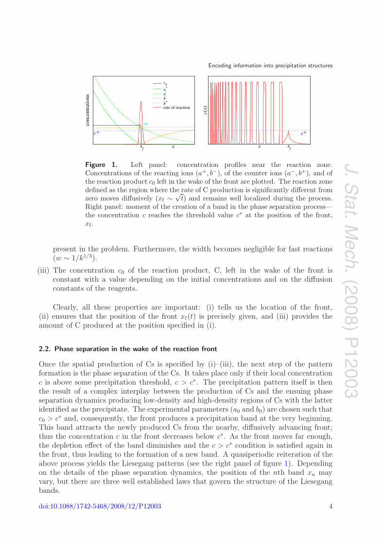
Figure 1. Left panel: concentration profiles near the reaction zone.Concentrations of the reacting ions (a+, b−), of the counter ions (a−, b+), and ofthe reaction product c0 left in the wake of the front are plotted. The reaction zonedefined as the region where the rate of C production is significantly different fromzero moves diffusively (xf ∼ √

t) and remains well localized during the process.Right panel: moment of the creation of a band in the phase separation process—the concentration c reaches the threshold value c∗ at the position of the front,xf .

present in the problem. Furthermore, the width becomes negligible for fast reactions(w ∼ 1/k1/3).

(iii) The concentration c0 of the reaction product, C, left in the wake of the front isconstant with a value depending on the initial concentrations and on the diffusionconstants of the reagents.

Clearly, all these properties are important: (i) tells us the location of the front,(ii) ensures that the position of the front xf(t) is precisely given, and (iii) provides theamount of C produced at the position specified in (i).

2.2. Phase separation in the wake of the reaction front

Once the spatial production of Cs is specified by (i)–(iii), the next step of the patternformation is the phase separation of the Cs. It takes place only if their local concentrationc is above some precipitation threshold, c > c∗. The precipitation pattern itself is thenthe result of a complex interplay between the production of Cs and the ensuing phaseseparation dynamics producing low-density and high-density regions of Cs with the latteridentified as the precipitate. The experimental parameters (a0 and b0) are chosen such thatc0 > c∗ and, consequently, the front produces a precipitation band at the very beginning.This band attracts the newly produced Cs from the nearby, diffusively advancing front;thus the concentration c in the front decreases below c∗. As the front moves far enough,the depletion effect of the band diminishes and the c > c∗ condition is satisfied again inthe front, thus leading to the formation of a new band. A quasiperiodic reiteration of theabove process yields the Liesegang patterns (see the right panel of figure 1). Dependingon the details of the phase separation dynamics, the position of the nth band xn mayvary, but there are three well established laws that govern the structure of the Liesegangbands.

doi:10.1088/1742-5468/2008/12/P12003 4

J.Stat.M

ech.(2008)

P12003

Encoding information into precipitation structures

(a) Time law [18]: the position of the nth band xn (measured from the initial interface ofthe reagents) is given by xn =

√2Dftn, where tn is the time of creation of the band.

(b) Spacing law [19]: the positions of the bands form a geometric series xn ∼ (1 + p)n

with a spacing coefficient p > 0, such that distances between successive bands increasewith the band index n.

(c) Width law [20]: the width of the nth band wn is proportional to its position: wn ∼ xn.

The above laws can be derived [15] by using the Cahn–Hilliard equation [21] fordescribing of the phase separation process. This approach also allows one to demonstratethat the band positions can be controlled by a0 or b0 since p in the spacing law depends onthese quantities (p ∼ 1/a0 is the so called Matalon–Packter law [22]). Unfortunately, thepossible changes are rather limited since the band positions invariably form a geometricseries.

3. Description of the control tool

3.1. Main idea—controlling the motion of the reagents by means of an electric current

Equipped with the understanding of both the front motion and the precipitation processes,we can start to think of possible control mechanisms. There are basically two ways tochange the structure of the pattern characterized by the spacing law (b) and the widthlaw (c). First, one can try to change the functional form of the time law (a). This can bedone by using various geometries or patterns in the initial state [5, 8, 10, 23], by controllingthe precipitation threshold [24], by employing guiding temperature or pH fields [11], orby considering systems where the diffusion of the reacting species is anomalous [25, 26].Unfortunately, these methods are rather unwieldy and are not flexible enough for easilycreating arbitrary patterns.

The second method keeps the time law unchanged and aims at controlling the creationtime tn of the nth band. Recalling that tn is the instant when the concentration of Cscrosses the threshold value c∗, one recognizes that tn can be controlled by regulatingthe concentration c0(x) at the front. Recently, it was shown both theoretically andexperimentally that the above method can be made to work by sending a time-dependentelectric current through the system [12]. The schematic setup for control is shown infigure 2 and, at a phenomenological level, its working can be understood rather easily.Indeed, consider an imposed current which drives the reacting ions towards the reactionzone (we shall refer to this current as the forward current). It is clear that the forwardcurrent enhances the production of Cs in the reaction zone. Reversing the direction ofcurrent (the backward current), on the other, hand works against the reaction and resultsin a lower production of Cs. Thus, provided the position of the front is known (i.e. xn(t)is available from the time law), the times tn of crossing of the threshold concentrationand, consequently, the positions of the band xn(tn) can be controlled by means of anappropriately chosen current. Since managing the electric current is not an experimentaldifficulty, the above method provides us with a flexible technique for the creation ofcomplex precipitation patterns.

doi:10.1088/1742-5468/2008/12/P12003 5

J.Stat.M

ech.(2008)

P12003

Encoding information into precipitation structures

Figure 2. Experimental setup for producing Liesegang precipitation patterns asdescribed in section 2.1. The controlling agent is the generator providing electriccurrent I(t) with a prescribed time dependence (this figure is taken from [12]).

3.2. Mathematical description of the process

For a more quantitative description of the control-by-current method, we shall usea mean field model that has been developed in a series of papers during the lastdecade [12, 15, 27, 28]. The first part of the model addresses the irreversible A+ +B− → C reaction–diffusion process for totally dissociated electrolytes A ≡ (A+, A−)and B ≡ (B+, B−) that are initially separated in space. The evolution equations forthe concentration profile of the ions a±(x, t) and b±(x, t) are obtained by assumingelectroneutrality on the relevant time and length scales [27] and, for the case of monovalentions with equal diffusion coefficients, the equations are as follows [12]:

∂ta+ = D∂2

xa+ − j(t) ∂x(a

+/Σ) − ka+b− (1)

∂tb− = D∂2

xb− + j(t) ∂x(b

−/Σ) − ka+b− (2)

∂ta− = D∂2

xa− + j(t) ∂x(a

−/Σ) (3)

∂tb+ = D∂2

xb+ − j(t) ∂x(b

+/Σ). (4)

Here D is the diffusion coefficient of the ions, j(t) = I(t)/A is the externally controlledelectric current density flowing through the tube of cross section A, and Σ = q(a+ + a− +b+ +b−) with q being the unit of charge. The reaction rate k is taken to be large, resultingin a reaction zone of negligible width. Note that this assumption is compatible with thetypical reactions used in experimental setups producing Liesegang structures.

The second part of the model explains the pattern formation through the separationof the reaction product C into high- and low-concentration phases. The evolution of theconcentration c(x, t) is obtained from the Cahn–Hilliard equation with the addition of asource term corresponding to the rate of the production of Cs (ka+b−) [15, 28]. The freeenergy driving the phase separation is assumed to have minima at some low (cl) and high(ch) concentrations of C and, furthermore, it is assumed to have the Landau–Ginzburgform in the shifted and rescaled concentration variable m = (2c − ch − cl)/(ch − cl). Interms of m, the equation describing the phase separation dynamics takes the form [15]

∂tm = −λΔ(m − m3 + σΔm) + S(x, t). (5)

doi:10.1088/1742-5468/2008/12/P12003 6

J.Stat.M

ech.(2008)

P12003

Encoding information into precipitation structures

Figure 3. Left panel: the position of the reaction front (measured in units of thelength L of the gel column) versus diffusion length in the absence of a current,displayed for constant forward or backward current, and for a quasiperiodiccurrent (changed at times τn2). Right panel: concentrations of the reactionproduct in the wake of the front for the cases considered in the left panel [12].

Here S(x, t) = 2ka+b−/(ch − cl) is the source term coming from equations (1)–(4). Thetwo parameters λ and σ are fitting parameters at this stage; they can be chosen so as toreproduce the correct experimental time and length scales [29, 28].

Equations (1)–(5) are a closed set of equations for the concentrations of theelectrolytes (a±, b±) and of the reaction product c. Together with the specification ofthe initial and the boundary conditions, they provide the mathematical formulation ofthe problem. Below we shall consider numerical solutions of these equations which wereobtained by the classical fourth-order Runge–Kutta method.

3.3. Simulation results—properties of the front in the presence of a current

In order to obtain a more detailed understanding of the front dynamics, we studiedthe numerical solution of equation (1) with initial conditions of separated electrolytes[a±(x < 0, t = 0) = a0, a±(x > 0, t = 0) = 0, b±(x < 0, t = 0) = 0, b±(x > 0, t = 0) = b0],and monitored both the position of the front xf(t) and the rate of production S = kab ofthe Cs (a brief account of these simulations appeared in [12]). The physical parameters inthe equations were chosen to be close to the experimentally relevant values (a0/b0 = 100,D = 1.22 × 10−9 m2 s−1, σ = 10−8 m2, λ = 0.17 × 10−9 m2 s−1) and we consideredthe following scenarios for the current. The no current case was used to reproduce theknown front properties (i)–(iii). Constant forward and backward currents of amplitude|j| = 10 A m−2 were simulated to check whether the time law holds on the experimentallyrelevant time scales. Finally, we studied the most interesting case of an alternating currentof constant absolute value (|j| = 10 A m−2) with its sign changing in a square wave patternat times τn2, with n = 0, 1, 2, . . ., and τ fixing the time scale of the protocol.

The results are shown in figure 3. The left panel displays the front motion and showsthat in all cases the diffusive nature of the front is hardly changed, i.e. the time law(a) remains valid. On the other hand, as can be seen in the right panel of figure 3,the C production at the front is strongly influenced by the character of the appliedcurrent. Backward current leads to a decrease of the concentration of Cs left behindthe front, and c0(x) reaches values below the phase separation threshold c0(x) < c∗, thus

doi:10.1088/1742-5468/2008/12/P12003 7

J.Stat.M

ech.(2008)

P12003

Encoding information into precipitation structures

eliminating the possibility of precipitation. In contrast, the forward current increasesthe C production steeply and brings the system quickly into the unstable regime, thusinducing precipitation. It follows then that, in the case of a quasiperiodic current, thephase separation can be triggered and timed by switching on the forward field.

4. Pattern design

4.1. Controlling the spacing and the width of the bands

Once the front dynamics, summarized in figure 3, is understood, one can invent anappropriate current dynamics that results in e.g. equidistant band patterns [12]. Thewavelength d of the periodic pattern can be predesigned by switching on the forwardcurrents at times tn = (2n)2τ , where n = 0, 1, 2, . . . and τ = d2/8Df . If the desiredperiod d is smaller than half the local wavelength of the Liesegang pattern which wouldbe present without the current (see figure 1), then spurious bands may appear due to anatural increase of the concentration of Cs. This can be avoided, however, by switchingon the backward current when the front is halfway between xn and xn+1, i.e., at times(2n + 1)2τ .

One can also create more complex patterns both experimentally and theoretically [12].When creating patterns of several wavelengths, variable widths of the bands may alsobecome an important part of the patterns. The issue of the width control, treated below,is the novel aspect of the present paper.

Let us begin by finding an estimate of the width of the equidistant bands having aperiod d =

√8Dfτ . From simulations we know that even in the presence of current, the

position of the front is well approximated by xf(t) =√

2Dft where Df is given by [16]

Df = 2D

{erf−1

[a0/b0 − 1

a0/b0 + 1

]}2

. (6)

For a typical ratio of the initial concentrations of A and B, a0/b0 = 100, this yieldsDf = 5.43D, where D is the diffusion constant of the ions.

An important point now is that simulations of the equidistant case (i.e. when theforward current is switched on at times tn = (2n)2τ) reveal (see figure 4) that, althoughthe C production varies strongly within a period, the average concentration is practicallyequal to the zero-current one. This means that, for the estimation of the width, we canreplace the complicated function c0(x) by the result of the homogeneous production ofCs [17]:

c0(x) ≈ c0 = a01 + b0/a0

2√

πe−Df/(2D)

√2D

Df. (7)

For a0/b0 = 100 this yields c0/a0 ≈ 1.145 × 10−2.Using now the conservation of Cs, namely that the amount of Cs produced in a period

(d c0) is distributed into the high- and low-concentration regions of length w and d − w,the width of the bands, w, is calculated as

w =c0 − cl

ch − cld =

c0 − cl

ch − cl

√8Dfτ , (8)

doi:10.1088/1742-5468/2008/12/P12003 8

J.Stat.M

ech.(2008)

P12003

Encoding information into precipitation structures

Figure 4. C concentration in the wake of the front for the equidistant pattern(red dashed line) and its average over a region of distance d (red solid line) incomparison with the no current case (blue line).

Figure 5. Left panel: definition of the width w and the period d of the equidistantpattern. Right panel: dependence of the numerically obtained widths (red cross)and periods (blue cross) on τ in comparison with the theoretical prediction (solidlines).

and we find that the width depends on τ in the same way as the period. The width alsodepends on the diffusion constant of the front, Df , which, in turn, depends on the ratiosof initial concentrations a0/b0 as well as on the diffusion coefficients of the electrolytes.Most easily, however, the width can tuned via the initial concentration of A, a0, which isproportional to c0.

In figure 5 one can see the numerical verification of the above approximations for thewidth and the wavelength of the periodic pattern. The smaller the value of τ , the betterthe estimate, since for large values of τ we enter a regime where the deviations from thetime law (a) become significant.

4.2. Encoding information into precipitation structures

Since spacing and width can be controlled using a properly designed current, more complexstructures should be realizable. The pattern shown in figure 6 has been created using a

doi:10.1088/1742-5468/2008/12/P12003 9

J.Stat.M

ech.(2008)

P12003

Encoding information into precipitation structures

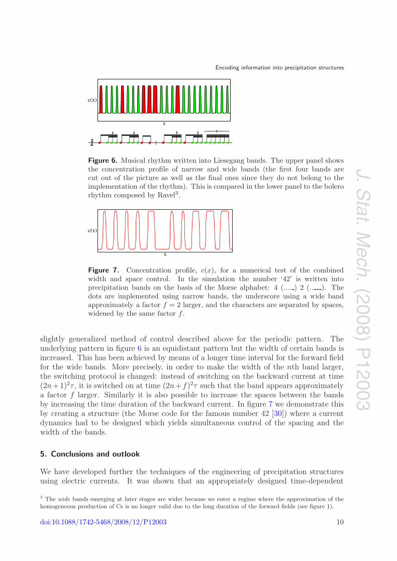
Figure 6. Musical rhythm written into Liesegang bands. The upper panel showsthe concentration profile of narrow and wide bands (the first four bands arecut out of the picture as well as the final ones since they do not belong to theimplementation of the rhythm). This is compared in the lower panel to the bolerorhythm composed by Ravel3.

Figure 7. Concentration profile, c(x), for a numerical test of the combinedwidth and space control. In the simulation the number ‘42’ is written intoprecipitation bands on the basis of the Morse alphabet: 4 (.... ) 2 (.. ). Thedots are implemented using narrow bands, the underscore using a wide bandapproximately a factor f = 2 larger, and the characters are separated by spaces,widened by the same factor f .

slightly generalized method of control described above for the periodic pattern. Theunderlying pattern in figure 6 is an equidistant pattern but the width of certain bands isincreased. This has been achieved by means of a longer time interval for the forward fieldfor the wide bands. More precisely, in order to make the width of the nth band larger,the switching protocol is changed: instead of switching on the backward current at time(2n+1)2τ , it is switched on at time (2n+f)2τ such that the band appears approximatelya factor f larger. Similarly it is also possible to increase the spaces between the bandsby increasing the time duration of the backward current. In figure 7 we demonstrate thisby creating a structure (the Morse code for the famous number 42 [30]) where a currentdynamics had to be designed which yields simultaneous control of the spacing and thewidth of the bands.

5. Conclusions and outlook

We have developed further the techniques of the engineering of precipitation structuresusing electric currents. It was shown that an appropriately designed time-dependent

3 The wide bands emerging at later stages are wider because we enter a regime where the approximation of thehomogeneous production of Cs is no longer valid due to the long duration of the forward fields (see figure 1).

doi:10.1088/1742-5468/2008/12/P12003 10

J.Stat.M

ech.(2008)P

12003

Encoding information into precipitation structures

current allows us to control not only the band spacing but also the width of the bandsin one-dimensional structures. This permits the encoding of information by controllingeither only the width (as exemplified by the bolero rhythm) or by combining the widthand space control (as was shown on the example of the famous number 42).

A naturally arising question concerns the limits of the approach when trying todownscale the structures. As far as the time scales are considered, since the diffusioncoefficients of the participating agents are of order 10−9 m2 s−1, imposed currents on thetime scale of τ = 0.1 s provide control on length scales of 10 μ m. Thus scaling thedynamics of the current does not pose an experimental problem.

The real problem with downscaling is the width of the bands. The minimum widthis clearly related to the width of the reaction front which is not negligible on the scaleof microns and, depending on the reagents, can be even at the scale of millimeters [31].It should be noted however that spontaneous pattern formation on the nanoscale levelhas been observed [32], and such systems might be appropriate for pattern control usingimposed electric currents. Another problem with the width of the bands is that thethermal fluctuations in the concentrations of the reagents combined with those of thegel make the reaction front uneven and, depending on the surface tension of the createdbands, they may lead to a roughening of the band on a scale that is comparable to thewidth. Difficulties in designing the details of the patterns may also arise because thepresence of the precipitate may significantly alter the transport of the reagents. Clearly,advances in downscaling can be achieved only if models are developed which can treat allthe above problems.

Finally, we note that combining the proposed technique with the already existingindirect control strategies such as the choice of geometry and initial conditions or re-dissolution methods [33] opens up a wide spectrum of possible structure design. Sofar the feasibility of the approach has only been shown for a few kinds of predesignedone-dimensional patterns. A straightforward extension would be the creation of ringsor spheres with a predesigned internal structure. Further, the extension of the current-control technique to stamping methods [5] on the mesoscopic level could be used to createeven more complex pattern designs which may become useful in engineering applications.

Acknowledgments

This work has been partly supported by the Swiss National Science Foundation and bythe Hungarian Academy of Sciences (Grant No. OTKA K68109).

References

[1] Shinbrot T and Muzzio F J, Noise to order , 2001 Nature 410 251[2] For a review see Cross M C and Hohenberg P C, Pattern formation outside of equilibrium, 1994 Rev. Mod.

Phys. 65 851[3] Henisch H K, 1991 Periodic Precipitation (New York: Pergamon)[4] Lu W and Lieber C M, Nanoelectronics from the bottom up, 2007 Nat. Mater. 6 841[5] Bensemann I T, Fialkowski M and Grzybowski B A, Wet stamping of microscale periodic precipitation

patterns, 2005 J. Phys. Chem. B 109 2774[6] Campbell C J, Baker E, Fialkowski M, Bitner A, Smoukov S K and Grzybowski B A, Self-organization of

planar microlenses by periodic precipitation, 2005 J. Appl. Phys. 97 126102[7] Maselko J, Self-organization as a new method for synthesizing smart and structured materials, 1996 Mater.

Sci. Eng. C 4 199

doi:10.1088/1742-5468/2008/12/P12003 11

J.Stat.M

ech.(2008)

P12003

Encoding information into precipitation structures

[8] Giraldo O, Brock S L, Marquez M, Suib S L, Hillhouse H and Tsapatsis M, Spontaneous formation ofinorganic helices, 2000 Nature 405 38

[9] Grzybowski B A and Campbell C J, Fabrication with programmable chemical reactions, 2007 Mater. Today10 38

[10] Lebedeva M I, Vlachos D G and Tsapatsis M, Bifurcation analysis of Liesegang ring pattern formation,2004 Phys. Rev. Lett. 92 088301

[11] Antal T, Bena I, Droz M, Martens K and Racz Z, Guiding fields for phase separation: controlling Liesegangpatterns, 2007 Phys. Rev. E 76 046203

[12] Bena I, Droz M, Lagzi I, Martens K, Racz Z and Volford A, Designer patterns: flexible control ofprecipitation through electric currents, 2008 Phys. Rev. Lett. 101 075701

[13] Liesegang R E, Ueber einige Eigenschaften von Gallerten, 1896 Naturwiss. Wochenschr. 11 353[14] Dee G T, Patterns produced by precipitation at a moving reaction front, 1986 Phys. Rev. Lett. 57 275[15] Antal T, Droz M, Magnin J and Racz Z, Formation of Liesegang patterns: a spinodal decomposition

scenario, 1999 Phys. Rev. Lett. 83 2880[16] Galfi L and Racz Z, Properties of the reaction front in an A + B → C type reaction–diffusion process, 1988

Phys. Rev. A 38 3151[17] Antal T, Droz M, Magnin J, Racz Z and Zrinyi M, Derivation of the Matalon–Packter law for Liesegang

patterns, 1998 J. Chem. Phys. 109 9479[18] Morse H W and Pierce G W, Diffusion and supersaturation in gelatine, 1903 Proc. Am. Acad. Arts. Sci. 38

625[19] Jablczynski K, La formation rhythmique des precipites: Les anneaux de Liesegang , 1923 Bull. Soc. Chim.

France 33 1592[20] Muller S C, Kai S and Ross J, Periodic precipitation patterns in the presence of concentration gradients. 1.

Dependence on ion product and concentration difference, 1982 J. Phys. Chem. 86 4078[21] Cahn J W and Hilliard J E, Free energy of a nonuniform system. I. Interfacial free energy , 1958 J. Chem.

Phys. 28 258Cahn J W, On spinodal decomposition, 1961 Acta Metall. 9 795

[22] Matalon R and Packter A, The Liesegang phenomenon I. Sol protection and diffusion, 1955 J. Colloid Sci.10 46

Packter A, The Liesegang phenomenon. IV: Reprecipitation from ammonia peptised sols, 1955 Kolloid Z.142 109

[23] Bena I, Droz M, Martens K and Racz Z, Reaction–diffusion fronts with inhomogeneous initial conditions,2007 J. Phys.: Condens. Matter 19 065103

[24] Molnar F Jr, Izsak F and Lagzi I, Design of equidistant and revert type precipitation patterns inreaction–diffusion systems, 2008 Phys. Chem. Chem. Phys. 10 2368

[25] Yuste S B, Acedo L and Lindenberg K, Reaction front in an A + B → C reaction–subdiffusion process, 2004Phys. Rev. E 69 036126

[26] Rongy L, Trevelyan P M J and De Wit A, Dynamics of A + B → C reaction fronts in the presence ofbuoyancy-driven convection, 2008 Phys. Rev. Lett. 101 084503

[27] Bena I, Coppex F, Droz M and Racz Z, Front motion in an A + B → C type reaction–diffusion process:effects of an electric field , 2005 J. Chem. Phys. 122 024512

[28] Bena I, Droz M and Racz Z, Formation of Liesegang patterns in the presence of an electric field , 2005 J.Chem. Phys. 122 204502

[29] Racz Z, Formation of Liesegang patterns, 1999 Physica A 274 50[30] Adams D, 2002 The Hitchhiker’s Guide to the Galaxy (New York: Ballantine Books)[31] Koo Y-E L and Kopelman R, Space-and time-resolved diffusion-limited binary reaction kinetics in

capillaries: experimental observation of segregation, anomalous exponents, and depletion zone, 1991 J.Stat. Phys. 65 893

[32] Mohr C, Dubiel M and Hofmeister H, Formation of silver particles and periodic precipitate layers in silicateglass induced by thermally assisted hydrogen permeation, 2001 J. Phys.: Condens. Matter 13 525

[33] Msharrafieh M and Sultan R, Dynamics of a complex diffusion–precipitation–re-dissolution Liesegangpattern, 2006 Chem. Phys. Lett. 421 221

doi:10.1088/1742-5468/2008/12/P12003 12