Fletcher 2019 J. Stat. Mech. 2019 124021

J. Stat. M

ech. (2019) 124021

Plug in estimation in high dimensional linear inverse problems a rigorous analysis∗

Alyson K Fletcher1, Parthe Pandit2, Sundeep Rangan3, Subrata Sarkar4 and Philip Schniter4,5

1 Department of Statistics, UC Los Angeles, CA, United States of America2 Department of ECE, UC Los Angeles, CA, United States of America3 Department of ECE, NYU, New York, NY, United States of America4 Department of ECE, The Ohio State University, Columbus, OH, United

States of AmericaE-mail: [email protected], [email protected], [email protected],

[email protected] and [email protected]

Received 15 May 2019Accepted for publication 6 June 2019 Published 20 December 2019

Online at stacks.iop.org/JSTAT/2019/124021https://doi.org/10.1088/1742-5468/ab321a

Abstract. Estimating a vector x from noisy linear measurements Ax+w often requires use of prior knowledge or structural constraints on x for accurate reconstruction. Several recent works have considered combining linear least-squares estimation with a generic or ‘plug-in’ denoiser function that can be designed in a modular manner based on the prior knowledge about x. While these methods have shown excellent performance, it has been difficult to obtain rigorous performance guarantees. This work considers plug-in denoising combined with the recently-developed vector approximate message passing (VAMP) algorithm, which is itself derived via expectation propagation techniques. It shown that the mean squared error of this ‘plug-and-play’ VAMP can be exactly predicted for high-dimensional right-rotationally invariant random A and Lipschitz denoisers. The method is demonstrated on applications in image recovery and parametric bilinear estimation.

Keywords: machine learning

S Supplementary material for this article is available online

A K Fletcher et al

Plug in estimation in high dimensional linear inverse problems a rigorous analysis

Printed in the UK

124021

JSMTC6

© 2019 IOP Publishing Ltd and SISSA Medialab srl

2019

19

J. Stat. Mech.

JSTAT

1742-5468

10.1088/1742-5468/ab321a

12

Journal of Statistical Mechanics: Theory and Experiment

© 2019 IOP Publishing Ltd and SISSA Medialab srl

ournal of Statistical Mechanics:J Theory and Experiment

IOP

∗ This article is an updated version of: Fletcher A K, Pandit P, Rangan S, Sarkar S and Schniter P 2018 Plug-in estimation in high-dimensional linear inverse problems: a rigorous analysis Advances in Neural Information Processing Systems 31 ed S Bengio, H Wallach, H Larochelle, K Grauman, N Cesa-Bianchi and R Garnett (Red Hook, NY: Curran Associates, Inc) pp 7440–7449.5 Author to whom any correspondence should be addressed.

1742-5468/ 19 /124021+15$33.00


2https://doi.org/10.1088/1742-5468/ab321a

J. Stat. M

ech. (2019) 124021Contents

1. Introduction 2

2. Review of vector AMP 4

3. Extending the analysis to non-separable denoisers 53.1. Separable denoisers ..........................................................................................63.2. Group-based denoisers .....................................................................................63.3. Convolutional denoisers ...................................................................................73.4. Convolutional neural networks ........................................................................73.5. Singular-value thresholding (SVT) denoiser ....................................................7

4. Large system limit analysis 74.1. System model ...................................................................................................74.2. State evolution of VAMP ................................................................................8

5. Numerical experiments 105.1. Compressive image recovery ..........................................................................105.2. Bilinear estimation via lifting ........................................................................11

6. Conclusions 13Acknowledgments ................................................................................ 13

References 13

1. Introduction

The estimation of an unknown vector x0 ∈ RN from noisy linear measurements y of the form

y = Ax0 +w ∈ RM, (1)where A ∈ RM×N is a known transform and w is disturbance, arises in a wide-range of learning and inverse problems. In many high-dimensional situations, such as when the measurements are fewer than the unknown parameters (i.e. M ≪ N), it is essential to incorporate known structure on x0 in the estimation process. A fundamental chal-lenge is how to perform structured estimation of x0 while maintaining computational efficiency and a tractable analysis.

Approximate message passing (AMP), originally proposed in [1], refers to a powerful class of algorithms that can be applied to reconstruction of x0 from (1) that can eas-ily incorporate a wide class of statistical priors. In this work, we restrict our attention to w ∼ N (0,γ−1

w I), noting that AMP was extended to non-Gaussian measurements in


3https://doi.org/10.1088/1742-5468/ab321a

J. Stat. M

ech. (2019) 124021[2–4]. AMP is computationally efficient, in that it generates a sequence of estimates {xk}∞k=0 by iterating the steps

xk = g(rk,γk) (2a)

vk = y −Axk +N

M⟨∇g(rk,γk)⟩vk−1 (2b)

rk+1 = xk +ATvk, γk+1 =M/∥vk∥2, (2c)initialized with r0 = ATy, γ0 = M/∥y∥2, v−1 = 0, and assuming A is scaled so that ∥A∥2F ≈ N . In (2), g : RN × R → RN is an estimation function chosen based on prior

knowledge about x0, and ⟨∇g(r,γ)⟩ := 1N

∑Nn=1

∂gn(r,γ)∂rn

denotes the divergence of g(r,γ). For example, if x0 is known to be sparse, then it is common to choose g(·) to be the componentwise soft-thresholding function, in which case AMP iteratively solves the LASSO [5] problem.

Importantly, for large, i.i.d., sub-Gaussian random matrices A and Lipschitz denois-ers g(·), the performance of AMP can be exactly predicted by a scalar state evolution (SE), which also provides testable conditions for optimality [6–8]. The initial work [6, 7] focused on the case where g(·) is a separable function with identical comp-onents (i.e. [g(r,γ)]n = g(rn,γ) ∀n), while the later work [8] allowed non-separable g(·). Interestingly, these SE analyses establish the fact that

rk = x0 +N (0,I/γk), (3)leading to the important interpretation that g(·) acts as a denoiser. This interpreta-tion provides guidance on how to choose g(·). For example, if x is i.i.d. with a known prior, then (3) suggests to choose a separable g(·) composed of minimum mean-squared error (MMSE) scalar denoisers g(rn, γ) = E(xn|rn = xn +N (0, 1/γ)). In this case, [6, 7] established that, whenever the SE has a unique fixed point, the estimates xk generated by AMP converge to the Bayes optimal estimate of x0 from y. As another example, if x is a natural image, for which an analytical prior is lacking, then (3) suggests to choose g(·) as a sophisticated image-denoising algorithm like BM3D [9] or DnCNN [10], as proposed in [11]. Many other examples of structured estimators g(·) can be considered; we refer the reader to [8] and section 5. Prior to [8], AMP SE results were established for special cases of g(·) in [12, 13]. Plug-in denoisers have been combined in related algorithms [14–16].

An important limitation of AMP’s SE is that it holds only for large, i.i.d., sub-Gaussian A. AMP itself often fails to converge with small deviations from i.i.d. sub-Gaussian A, such as when A is mildly ill-conditioned or non-zero-mean [4, 17, 18]. Recently, a robust alternative to AMP called vector AMP (VAMP) was proposed and analyzed in [19], based closely on expectation propagation [20]—see also [21–23]. There it was established that, if A is a large right-rotationally invariant random matrix and g(·) is a separable Lipschitz denoiser, then VAMP’s performance can be exactly predicted by a scalar SE, which also provides testable conditions for optimal-ity. Importantly, VAMP applies to arbitrarily conditioned matrices A, which is a significant benefit over AMP, since it is known that ill-conditioning is one of AMP’s main failure mechanisms [4, 17, 18].


4https://doi.org/10.1088/1742-5468/ab321a

J. Stat. M

ech. (2019) 124021

Unfortunately, the SE analyses of VAMP in [24] and its extension in [25] are limited to separable denoisers. This limitation prevents a full understanding of VAMP’s behavior when used with non-separable denoisers, such as state-of-the-art image-denoising meth-ods as recently suggested in [26]. The main contribution of this work is to show that the SE analysis of VAMP can be extended to a large class of non-separable denoisers that are Lipschitz continuous and satisfy a certain convergence property. The conditions are simi-lar to those used in the analysis of AMP with non-separable denoisers in [8]. We show that there are several interesting non-separable denoisers that satisfy these conditions, including group-structured and convolutional neural network based denoisers.

An extended version with all proofs and other details are provided in [27].

2. Review of vector AMP

The steps of VAMP algorithm of [19] are shown in algorithm 1. Each iteration has two parts: a denoiser step and a linear MMSE (LMMSE) step. These are characterized by estimation functions g1(·) and g2(·) producing estimates x1k and x2k. The estimation functions take inputs r1k and r2k that we call partial estimates. The LMMSE estimation function is given by,

g2(r2k,γ2k) :=(γwA

TA+ γ2kI)−1 (

γwATy + γ2kr2k

), (4)

where γw > 0 is a parameter representing an estimate of the precision (inverse variance) of the noise w in (1). The estimate x2k is thus an MMSE estimator, treating the x as having a Gaussian prior with mean given by the partial estimate r2k. The estimation function g1(·) is called the denoiser and can be designed identically to the denoiser g(·) in the AMP iterations (2). In particular, the denoiser is used to incorporate the

Algorithm 1. Vector AMP (LMMSE form).

Require: LMMSE estimator g2(·,γ2k) from (4), denoiser g1(·,γ1k), and number of iterations Kit.1: Select initial r10 and γ10 ! 0.2: for k = 0, 1, . . . ,Kit do3: // Denoising4: x1k = g1(r1k,γ1k)5: α1k = ⟨∇g1(r1k,γ1k)⟩6: η1k = γ1k/α1k, γ2k = η1k − γ1k7: r2k = (η1kx1k − γ1kr1k)/γ2k8:9: // LMMSE estimation10: x2k = g2(r2k,γ2k)

11: α2k = ⟨∇g2(r2k,γ2k)⟩12: η2k = γ2k/α2k, γ1,k+1 = η2 k − γ2 k

13: r1,k+1 = (η2 kx2 k − γ2 kr2 k)/γ1,k+114: end for15: Return x1Kit.


5https://doi.org/10.1088/1742-5468/ab321a

J. Stat. M

ech. (2019) 124021structural or prior information on x. As in AMP, in lines 5 and 11, ⟨∇gi⟩ denotes the normalized divergence.

The main result of [24] is that, under suitable conditions, VAMP admits a state evolution (SE) analysis that precisely describes the mean squared error (MSE) of the estimates x1k and x2k in a certain large system limit (LSL). Importantly, VAMP’s SE analysis applies to arbitrary right rotationally invariant A. This class is considerably larger than the set of sub-Gaussian i.i.d. matrices for which AMP applies. However, the SE analysis in [24] is restricted separable Lipschitz denoisers that can be described as follows: let g1n(r1,γ1) be the nth component of the output of g1(r1,γ1). Then, it is assumed that,

x1n = g1n(r1,γ1) = φ(r1n,γ1), (5)for some function scalar-output function φ(·) that does not depend on the component index n. Thus, the estimator is separable in the sense that the nth component of the estimate, x1n depends only on the nth component of the input r1n as well as the preci-sion level γ1. In addition, it is assumed that φ(r1,γ1) satisfies a certain Lipschitz con-dition. The separability assumption precludes the analysis of more general denoisers mentioned in the introduction.

3. Extending the analysis to non-separable denoisers

The main contribution of the paper is to extend the state evolution analysis of VAMP to a class of denoisers that we call uniformly Lipschitz and convergent under Gaussian noise. This class is significantly larger than separable Lipschitz denoisers used in [24]. To state these conditions precisely, consider a sequence of estimation problems, indexed by a vector dimension N. For each N, suppose there is some ‘true’ vector u = u(N) ∈ RN that we wish to estimate from noisy measurements of the form, r = u+ z, where z ∈ RN is Gaussian noise. Let u = g(r,γ) be some estimator, parameterized by γ.

Definition 1. The sequence of estimators g(·) are said to be uniformly Lipschitz con-tinuous if there exists constants A, B and C > 0, such that

∥g(r2,γ2)− g(r1,γ1)∥ ! (A+ B|γ2 − γ1|)∥r2 − r1∥+ C√N |γ2 − γ1|, (6)

for any r1, r2, γ1, γ2 and N.

Definition 2. The sequence of random vectors u and estimators g(·) are said to be convergent under Gaussian noise if the following condition holds: let z1, z2 ∈ RN be two sequences where (z1n,z2n) are i.i.d. with (z1n, z2n) = N (0,S) for some positive definite covariance S ∈ R2×2. Then, all the following limits exist almost surely:

limN→∞

1

Ng(u+ z1, γ1)

Tg(u+ z2, γ2), limN→∞

1

Ng(u+ z1, γ1)

Tu, (7a)

limN→∞

1

NuTz1, lim

N→∞

1

N∥u∥2 (7b)


6https://doi.org/10.1088/1742-5468/ab321a

J. Stat. M

ech. (2019) 124021lim

N→∞⟨∇g(u+ z1,γ1)⟩ =

1

NS12g(u+ z1,γ1)

Tz2, (7c)

for all γ1, γ2 and covariance matrices S. Moreover, the values of the limits are continu-ous in S, γ1 and γ2.

With these definitions, we make the following key assumption on the denoiser.

Assumption 1. For each N, suppose that we have a ‘true’ random vector x0 ∈ RN and a denoiser g1(r1,γ1) acting on signals r1 ∈ RN . Following definition 1, we assume the sequence of denoiser functions indexed by N, is uniformly Lipschitz continuous. In addition, the sequence of true vectors x0 and denoiser functions are convergent under Gaussian noise following definition 2.

The first part of assumption 1 is relatively standard: Lipschitz and uniform Lipschitz continuity of the denoiser is assumed several AMP-type analyses including [6, 24, 28] What is new is the assumption in definition 2. This assumption relates to the behavior of the denoiser g1(r1,γ1) in the case when the input is of the form, r1 = x0 + z. That is, the input is the true signal with a Gaussian noise perturbation. In this setting, we will be requiring that certain correlations converge. Before continuing our analysis, we briefly show that separable denoisers as well as several interesting non-separable denoisers satisfy these conditions.

3.1. Separable denoisers

We first show that the class of denoisers satisfying assumption 1 includes the sepa-rable Lipschitz denoisers studied in most AMP analyses such as [6]. Specifically, sup-pose that the true vector x0 has i.i.d. components with bounded second moments and the denoiser g1(·) is separable in that it is of the form (5). Under a certain uniform Lipschitz condition, it is shown in the extended version of this paper [27] that the denoiser satisfies assumption 1.

3.2. Group-based denoisers

As a first non-separable example, let us suppose that the vector x0 can be represented as an L×K matrix. Let x0

ℓ ∈ RK denote the ℓth row and assume that the rows are i.i.d. Each row can represent a group. Suppose that the denoiser g1(·) is groupwise separable. That is, if we denote by g1ℓ(r,ℓ) the ℓth row of the output of the denoiser, we assume that

g1ℓ(r,γ) = φ(rℓ,γ) ∈ RK, (8)for a vector-valued function φ(·) that is the same for all rows. Thus, the ℓth row output gℓ(·) depends only on the ℓth row input. Such groupwise denoisers have been used in AMP and EP-type methods for group LASSO and other structured estimation prob-lems [29–31]. Now, consider the limit where the group size K is fixed, and the number of groups L → ∞. Then, under suitable Lipschitz continuity conditions, the extended version of this paper [27] shows that groupwise separable denoiser also satisfies assump-tion 1.


7https://doi.org/10.1088/1742-5468/ab321a

J. Stat. M

ech. (2019) 1240213.3. Convolutional denoisers

As another non-separable denoiser, suppose that, for each N, x0 is an N sample seg-ment of a stationary, ergodic process with bounded second moments. Suppose that the denoiser is given by a linear convolution,

g1(r1) := TN(h ∗ r1), (9)where h is a finite length filter and TN(·) truncates the signal to its first N samples. For simplicity, we assume there is no dependence on γ1. Convolutional denoising arises in many standard linear estimation operations on wide sense stationary processes such as Weiner filtering and smoothing [32]. If we assume that h remains constant and N → ∞, the extended version of this paper [27] shows that the sequence of random vectors x0 and convolutional denoisers g1(·) satisfies assumption 1.

3.4. Convolutional neural networks

In recent years, there has been considerable interest in using trained deep convolutional neural networks for image denoising [33, 34]. As a simple model for such a denoiser, suppose that the denoiser is a composition of maps,

g1(r1) = (FL ◦ FL−1 ◦ · · · ◦ F1)(r1), (10)where Fℓ(·) is a sequence of layer maps where each layer is either a multi-channel convolutional operator or Lipschitz separable activation function, such as sigmoid or ReLU. Under mild assumptions on the maps, it is shown in the extended version of this paper [27] that the estimator sequence g1(·) can also satisfy assumption 1.

3.5. Singular-value thresholding (SVT) denoiser

Consider the estimation of a low-rank matrix X0 from linear measurements y = A(X0),

where A is some linear operator [35]. Writing the SVD of R as R =∑

i σiuivTi , the

SVT denoiser is defined as

g1(R,γ) :=∑

i

(σi − γ)+uivTi , (11)

where (x)+ := max{0,x}. In the extended version of this paper [27], we show that g1(·) satisfies assumption 1.

4. Large system limit analysis

4.1. System model

Our main theoretical contribution is to show that the SE analysis of VAMP in [19] can be extended to the non-separable case. We consider a sequence of problems indexed by the vector dimension N. For each N, we assume that there is a ‘true’ random vector x0 ∈ RN observed through measurements y ∈ RM of the form in (1) where


8https://doi.org/10.1088/1742-5468/ab321a

J. Stat. M

ech. (2019) 124021w ∼ N (0,γ−1

w0I). We use γw0 to denote the ‘true’ noise precision to distinguish this from the postulated precision, γw, used in the LMMSE estimator (4). Without loss of gener-ality (see below), we assume that M = N. We assume that A has an SVD,

A = USVT, S = diag(s), s = (s1,. . . ,sN), (12)where U and V are orthogonal and S is non-negative and diagonal. The matrix U is arbitrary, s is an i.i.d. random vector with components si ∈ [0, smax] almost surely. Importantly, we assume that V is Haar distributed, meaning that it is uniform on the N ×N orthogonal matrices. This implies that A is right rotationally invariant meaning that A

d= AV0 for any orthogonal matrix V0. We also assume that w, x0, s and V are

all independent. As in [19], we can handle the case of rectangular V by zero padding s.These assumptions are similar to those in [19]. The key new assumption is assump-

tion 1. Given such a denoiser and postulated variance γw, we run the VAMP algorithm, algorithm 1. We assume that the initial condition is given by,

r = x0 +N (0,τ10I), (13)for some initial error variance τ10. In addition, we assume

limN→∞

γ10 = γ10, (14)almost surely for some γ10 ! 0.

Analogous to [24], we define two key functions: error functions and sensitivity func-tions. The error functions characterize the MSEs of the denoiser and LMMSE estimator under AWGN measurements. For the denoiser g1(·,γ1), we define the error function as

E1(γ1,τ1) := limN→∞

1

N∥g1(x

0 + z,γ1)− x0∥2, z ∼ N (0,τ1I), (15)

and, for the LMMSE estimator, as

E2(γ2,τ2) := limN→∞

1

NE∥g2(r2,γ2)− x0∥2,

r2 = x0 +N (0,τ2I), y = Ax0 +N (0,γ−1w0I).

(16)

The limit (15) exists almost surely due to the assumption of g1(·) being convergent under Gaussian noise. Although E2(γ2,τ2) implicitly depends on the precisions γw0 and γw, we omit this dependence to simplify the notation. We also define the sensitivity functions as

Ai(γi,τi) := limN→∞

⟨∇gi(x0 + zi,γi)⟩, zi ∼ N (0,τiI). (17)

The LMMSE error function (16) and sensitivity functions (17) are identical to those in the VAMP analysis [19]. The denoiser error function (15) generalizes the error func-tion in [19] for non-separable denoisers.

4.2. State evolution of VAMP

We now show that the VAMP algorithm with a non-separable denoiser follows the identical state evolution equations as the separable case given in [19]. Define the error vectors,


9https://doi.org/10.1088/1742-5468/ab321a

J. Stat. M

ech. (2019) 124021pk := r1k − x0, qk := VT(r2k − x0). (18)

Thus, pk represents the error between the partial estimate r1k and the true vector x0. The error vector qk represents the transformed error r2k − x0. The SE analysis will show that these errors are asymptotically Gaussian. In addition, the analysis will exactly predict the variance on the partial estimate errors (18) and estimate errors, xi − x0. These variances are computed recursively through what we will call the state evolution equations:

α1k = A1(γ1k,τ1k), η1k =γ1k

α1k, γ2k = η1k − γ1k (19a)

τ2k =1

(1− α1k)2[E1(γ1k,τ1k)− α2

1kτ1k], (19b)

α2 k = A2 (γ2 k,τ2 k), η2 k =γ2 kα2 k, γ1,k+1 = η2 k − γ2 k (19c)

τ1,k+1 =1

(1− α2 k)2[E2 (γ2 k,τ2 k)− α22 kτ2 k

], (19d)

which are initialized with k = 0, τ10 in (13) and γ10 defined from the limit (14). The SE equations in (19) are identical to those in [19] with the new error and sensitivity functions for the non-separable denoisers. We can now state our main result, which is proven in the extended version of this paper [27].Theorem 1. Under the above assumptions and definitions, assume that the sequence of true random vectors x0 and denoisers g1(r1,γ1) satisfy assumption 1. Assume ad-ditionally that, for all iterations k, the solution α1k from the SE equations (19) satisfies α1k ∈ (0, 1) and γik > 0. Then,

(a) For any k, the error vectors on the partial estimates, pk and qk in (18) can be written as,

pk = pk +O(1√N), qk = qk +O(

1√N), (20)

where, pk and qk ∈ RN are each i.i.d. Gaussian random vectors with zero mean and per component variance τ1k and τ2k, respectively.

(b) For any fixed iteration k ! 0, and i = 1, 2, we have, almost surely

limN→∞

1

N∥xi − x0∥2 = 1

ηik, lim

N→∞(αik, ηik, γik) = (αik, ηik, γik). (21)

In (20), we have used the notation, that when u, u ∈ RN are sequences of random vec-

tors, u = u+O( 1√N) means limN→∞

1N ∥u− u∥2 = 0 almost surely. Part (a) of theorem

1 thus shows that the error vectors pk and qk in (18) are approximately i.i.d. Gaussian.


10https://doi.org/10.1088/1742-5468/ab321a

J. Stat. M

ech. (2019) 124021The result is a natural extension to the main result on separable denoisers in [19]. Moreover, the variance on the variance on the errors, along with the mean squared error (MSE) of the estimates xik can be exactly predicted by the same SE equations as the separable case. The result thus provides an asymptotically exact analysis of VAMP extended to non-separable denoisers.

5. Numerical experiments

5.1. Compressive image recovery

We first consider the problem of compressive image recovery, where the goal is to recover an image x0 ∈ RN from measurements y ∈ RM of the form (1) with M ≪ N . This problem arises in many imaging applications, such as magnetic resonance imaging, radar imaging, computed tomography, etc, although the details of A and x0 change in each case.

One of the most popular approaches to image recovery is to exploit sparsity in the wavelet transform coefficients c := Ψx0, where Ψ is a suitable orthonormal wavelet transform. Rewriting (1) as y = AΨc+w, the idea is to first estimate c from y (e.g. using LASSO) and then form the image estimate via x = ΨTc. Although many algo-rithms exist to solve the LASSO problem, the AMP algorithms are among the fast-est (see, e.g. [36, figure 1]). As an alternative to the sparsity-based approach, it was recently suggested in [11] to recover x0 directly using AMP (2) by choosing the estima-tion function g as a sophisticated image-denoising algorithm like BM3D [9] or DnCNN [10].

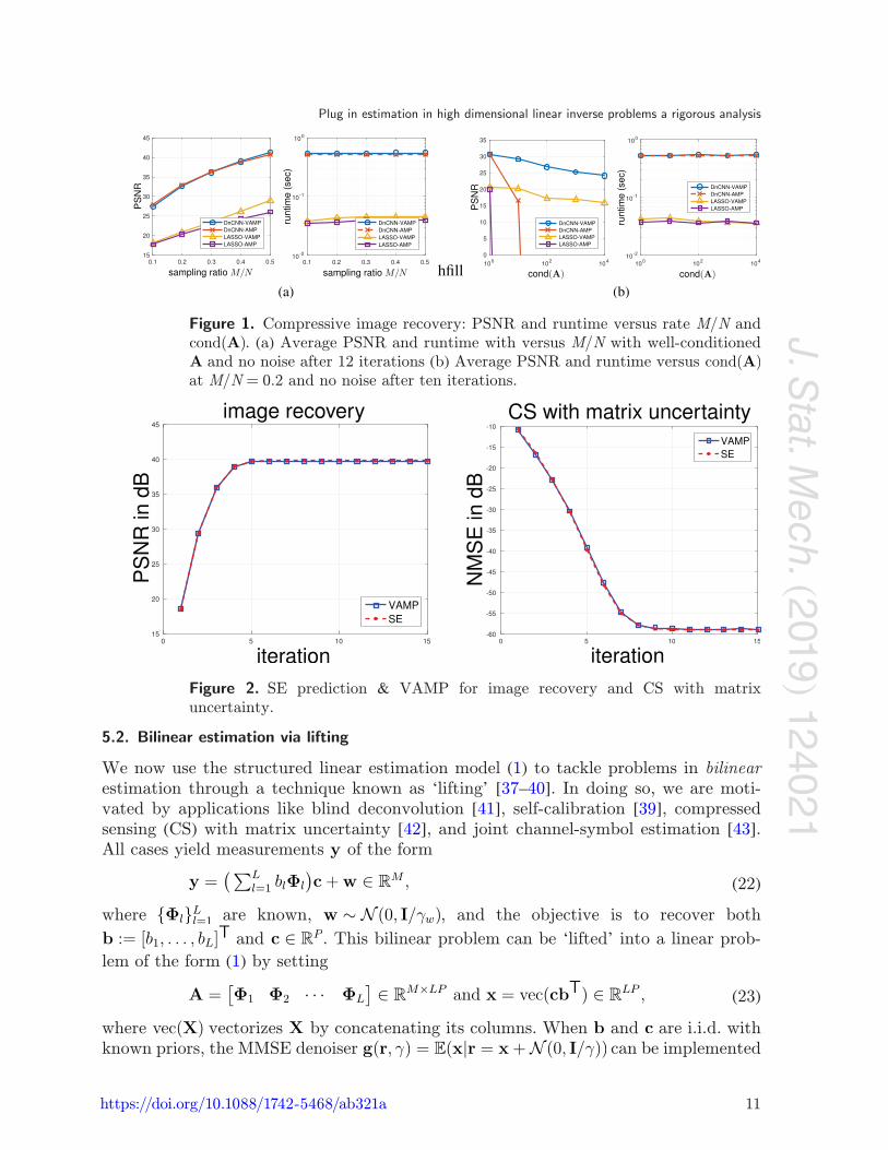
Figure 1(a) compares the LASSO- and DnCNN-based versions of AMP and VAMP for 128×128 image recovery under well-conditioned A and no noise. Here, A = JPHD, where D is a diagonal matrix with random ±1 entries, H is a discrete Hadamard trans-form (DHT), P is a random permutation matrix, and J contains the first M rows of IN. The results average over the well-known lena, barbara, boat, house, and peppers images using ten random draws of A for each. The figure shows that AMP and VAMP have very similar runtimes and PSNRs when A is well-conditioned, and that the DnCNN approach is about 10 dB more accurate, but 10× as slow, as the LASSO approach. Figure 2 shows the state-evolution prediction of VAMP’s PSNR on the barbara image at M/N = 0.5, averaged over 50 draws of A. The state-evolution accurately predicts the PSNR of VAMP.

To test the robustness to the condition number of A, we repeated the experi-ment from figure 1(a) using A = JDiag(s)PHD, where Diag(s) is a diagonal matrix of singular values. The singular values were geometrically spaced, i.e. sm/sm−1 = ρ ∀m, with ρ chosen to achieve a desired cond(A) := s1/sM. The sampling rate was fixed at M/N = 0.2, and the measurements were noiseless, as before. The results, shown in figure 1(b), show that AMP diverged when cond(A) ! 10, while VAMP exhibited only a mild PSNR degradation due to ill-conditioned A. The original images and example image recoveries are included in the extended version of this paper.


11https://doi.org/10.1088/1742-5468/ab321a

J. Stat. M

ech. (2019) 124021

5.2. Bilinear estimation via lifting

We now use the structured linear estimation model (1) to tackle problems in bilinear estimation through a technique known as ‘lifting’ [37–40]. In doing so, we are moti-vated by applications like blind deconvolution [41], self-calibration [39], compressed sensing (CS) with matrix uncertainty [42], and joint channel-symbol estimation [43]. All cases yield measurements y of the form

y =(∑L

l=1 blΦl

)c+w ∈ RM, (22)

where {Φl}Ll=1 are known, w ∼ N (0,I/γw), and the objective is to recover both

b := [b1, . . . , bL]T and c ∈ RP . This bilinear problem can be ‘lifted’ into a linear prob-lem of the form (1) by setting

A =[Φ1 Φ2 · · · ΦL

]∈ RM×LP and x = vec(cbT) ∈ RLP , (23)

where vec(X) vectorizes X by concatenating its columns. When b and c are i.i.d. with known priors, the MMSE denoiser g(r,γ) = E(x|r = x+N (0,I/γ)) can be implemented

Figure 1. Compressive image recovery: PSNR and runtime versus rate M/N and cond(A). (a) Average PSNR and runtime with versus M/N with well-conditioned A and no noise after 12 iterations (b) Average PSNR and runtime versus cond(A) at M/N = 0.2 and no noise after ten iterations.

Figure 2. SE prediction & VAMP for image recovery and CS with matrix uncertainty.


12https://doi.org/10.1088/1742-5468/ab321a

J. Stat. M

ech. (2019) 124021

near-optimally by the rank-one AMP algorithm from [44] (see also [45–47]), with diver-gence estimated as in [11].

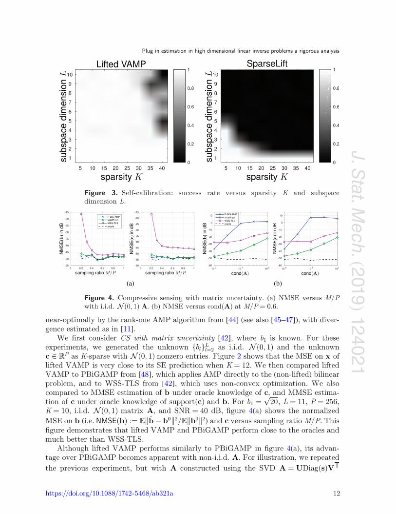
We first consider CS with matrix uncertainty [42], where b1 is known. For these experiments, we generated the unknown {bl}Ll=2 as i.i.d. N (0, 1) and the unknown c ∈ RP as K-sparse with N (0, 1) nonzero entries. Figure 2 shows that the MSE on x of lifted VAMP is very close to its SE prediction when K = 12. We then compared lifted VAMP to PBiGAMP from [48], which applies AMP directly to the (non-lifted) bilinear problem, and to WSS-TLS from [42], which uses non-convex optimization. We also compared to MMSE estimation of b under oracle knowledge of c, and MMSE estima-tion of c under oracle knowledge of support(c) and b. For b1 =

√20, L = 11, P = 256,

K = 10, i.i.d. N (0, 1) matrix A, and SNR = 40 dB, figure 4(a) shows the normalized MSE on b (i.e. NMSE(b) := E∥b− b0∥2/E∥b0∥2) and c versus sampling ratio M/P. This figure demonstrates that lifted VAMP and PBiGAMP perform close to the oracles and much better than WSS-TLS.

Although lifted VAMP performs similarly to PBiGAMP in figure 4(a), its advan-tage over PBiGAMP becomes apparent with non-i.i.d. A. For illustration, we repeated

the previous experiment, but with A constructed using the SVD A = UDiag(s)VT

Figure 3. Self-calibration: success rate versus sparsity K and subspace dimension L.

Figure 4. Compressive sensing with matrix uncertainty. (a) NMSE versus M/P with i.i.d. N (0, 1) A. (b) NMSE versus cond(A) at M/P = 0.6.


13https://doi.org/10.1088/1742-5468/ab321a

J. Stat. M

ech. (2019) 124021with Haar distributed U and V and geometrically spaced s. Also, to make the problem more difficult, we set b1 = 1. Figure 4(b) shows the normalized MSE on b and c versus cond(A) at M/P = 0.6. There it can be seen that lifted VAMP is much more robust than PBiGAMP to the conditioning of A.

We next consider the self-calibration problem [39], where the measurements take the form

y = Diag(Hb)Ψc+w ∈ RM. (24)Here the matrices H ∈ RM×L and Ψ ∈ RM×P are known and the objective is to recover the unknown vectors b and c. Physically, the vector Hb represents unknown calibra-tion gains that lie in a known subspace, specified by H. Note that (24) is an instance of (22) with Φl = Diag(hl)Ψ, where hl denotes the lth column of H. Different from ‘CS with matrix uncertainty,’ all elements in b are now unknown, and so WSS-TLS [42] cannot be applied. Instead, we compare lifted VAMP to the SparseLift approach from [39], which is based on convex relaxation and has provable guarantees. For our experiment, we generated Ψ and b ∈ RL as i.i.d. N (0, 1); c as K-sparse with N (0, 1) nonzero entries; H as randomly chosen columns of a Hadamard matrix; and w = 0. Figure 3 plots the success rate versus L and K, where ‘success’ is defined

as E∥cbT − c0(b0)T∥2F/E∥c0(b0)T∥2F < −60 dB. The figure shows that, relative to SparseLift, lifted VAMP gives successful recoveries for a wider range of L and K.

6. Conclusions

We have extended the analysis of the method in [24] to a class of non-separable denois-ers. The method provides a computational efficient method for reconstruction where structural information and constraints on the unknown vector can be incorporated in a modular manner. Importantly, the method admits a rigorous analysis that can provide precise predictions on the performance in high-dimensional random settings.

Acknowledgments

A K Fletcher and P Pandit were supported in part by the National Science Foundation under Grants 1738285 and 1738286 and the Office of Naval Research under Grant N00014-15-1-2677. S Rangan was supported in part by the National Science Foundation under Grants 1116589, 1302336, and 1547332, and the industrial affiliates of NYU WIRELESS. P Schniter and S Sarkar were supported in part by the National Science Foundation under Grant CCF-1716388.

References

[1] Donoho D L, Maleki A and Montanari A 2009 Message-passing algorithms for compressed sensing Proc. Natl Acad. Sci. 106 18914–9

[2] Rangan S 2011 Generalized approximate message passing for estimation with random linear mixing Proc. IEEE ISIT pp 2174–8


14https://doi.org/10.1088/1742-5468/ab321a

J. Stat. M

ech. (2019) 124021 [3] Rangan S, Schniter P, Riegler E, Fletcher A and Cevher V 2013 Fixed points of generalized approximate

message passing with arbitrary matrices Proc. IEEE ISIT pp 664–8 [4] Rangan S, Schniter P and Fletcher A K 2014 On the convergence of approximate message passing with

arbitrary matrices Proc. IEEE ISIT pp 236–40 [5] Tibshirani R 1996 Regression shrinkage and selection via the lasso J. R. Stat. Soc. B 58 267–88 [6] Bayati M and Montanari A 1996 The dynamics of message passing on dense graphs, with applications to

compressed sensing IEEE Trans. Inf. Theory 57 764–85 [7] Javanmard A and Montanari A 2013 State evolution for general approximate message passing algorithms,

with applications to spatial coupling Inf. Inference 2 115–44 [8] Berthier R, Montanari A and Nguyen P-M 2017 State evolution for approximate message passing with

non-separable functions (arXiv:1708.03950) [9] Dabov K, Foi A, Katkovnik V and Egiazarian K 2007 Image denoising by sparse 3-D transform-domain

collaborative filtering IEEE Trans. Image Process. 16 2080–95 [10] Zhang K, Zuo W, Chen Y, Meng D and Zhang L 2017 Beyond a Gaussian denoiser: residual learning of deep

CNN for image denoising IEEE Trans. Image Process. 26 3142–55 [11] Metzler C A, Maleki A and Baraniuk R G 2016 From denoising to compressed sensing IEEE Trans. Inf.

Theory 62 5117–44 [12] Donoho D, Johnstone I and Montanari A 2013 Accurate prediction of phase transitions in compressed

sensing via a connection to minimax denoising IEEE Trans. Inf. Theory 59 3396–433 [13] Ma Y, Rush C and Baron D 2017 Analysis of approximate message passing with a class of non-separable

denoisers Proc. ISIT pp 231–5 [14] Venkatakrishnan S V, Bouman C A and Wohlberg B 2013 Plug-and-play priors for model based

reconstruction Proc. IEEE Global Conf. on Signal and Inf. Processing pp 945–8 [15] Chen S, Luo C, Deng B, Qin Y, Wang H and Zhuang Z 2017 BM3D vector approximate message passing for

radar coded-aperture imaging PIERS-FALL pp 2035–8 [16] Wang X and Chan S H 2017 Parameter-free plug-and-play ADMM for image restoration Proc. IEEE

Acoustics, Speech and Signal Processing (IEEE) pp 1323–7 [17] Caltagirone F, Zdeborová L and Krzakala F 2014 On convergence of approximate message passing

Proc. IEEE ISIT pp 1812–6 [18] Vila J, Schniter P, Rangan S, Krzakala F and Zdeborová L 2015 Adaptive damping and mean removal for

the generalized approximate message passing algorithm Proc. IEEE ICASSP pp 2021–5 [19] Rangan S, Schniter P and Fletcher A K 2017 Vector approximate message passing Proc. IEEE ISIT

pp 1588–92 [20] Opper M and Winther O 2005 Expectation consistent approximate inference J. Mach. Learn. Res.

1 2177–204 [21] Fletcher A K, Sahraee-Ardakan M, Rangan S and Schniter P 2016 Expectation consistent approximate

inference: generalizations and convergence Proc. IEEE ISIT pp 190–4 [22] Ma J and Ping L 2017 Orthogonal AMP IEEE Access 5 2020–33 [23] Takeuchi K 2017 Rigorous dynamics of expectation-propagation-based signal recovery from unitarily

invariant measurements Proc. ISIT pp 501–5 [24] Rangan S, Schniter P and Fletcher A K 2016 Vector approximate message passing (arXiv:1610.03082) [25] Fletcher A K, Sahraee-Ardakan M, Rangan S and Schniter P 2017 Rigorous dynamics and consistent

estimation in arbitrarily conditioned linear systems Proc. NIPS pp 2542–51 [26] Schniter P, Fletcher A K and Rangan S 2017 Denoising-based vector AMP Proc. Int. Biomedical

and Astronomical Signal Process. Workshop pp 77 [27] Fletcher A K, Pandit P, Rangan S, Sarkar S and Schniter P 2018 Plug-in estimation in high-dimensional

linear inverse problems: a rigorous analysis (arXiv:1806.10466) [28] Kamilov U S, Rangan S, Fletcher A K and Unser M 2014 Approximate message passing with consistent

parameter estimation and applications to sparse learning IEEE Trans. Inf. Theory 60 2969–85 [29] Taeb A, Maleki A, Studer C and Baraniuk R 2013 Maximin analysis of message passing algorithms for recov-

ering block sparse signals (arXiv:1303.2389) [30] Andersen M R, Winther O and Hansen L K 2014 Bayesian inference for structured spike and slab priors

Advances in Neural Information Processing Systems (Red Hook, NY: Curran Associates, Inc.) pp 1745–53 [31] Rangan S, Fletcher A K, Goyal V K, Byrne E and Schniter P 2017 Hybrid approximate message passing

IEEE Trans. Signal Process. 65 4577–92 [32] Scharf L L and Demeure C 1991 Statistical signal Processing: Detection, Estimation, and Time Series

Analysis vol 63 (Reading, MA: Addison-Wesley) [33] Xie J, Xu L and Chen E 2012 Image denoising and inpainting with deep neural networks Advances in

Neural Information Processing Systems (Red Hook, NY: Curran Associates, Inc.) pp 341–9


15https://doi.org/10.1088/1742-5468/ab321a

J. Stat. M

ech. (2019) 124021 [34] Xu L, Ren J S, Liu C and Jia J 2014 Deep convolutional neural network for image deconvolution Advances

in Neural Information Processing Systems (Red Hook, NY: Curran Associates, Inc.) pp 1790–8 [35] Cai J-F, Candès E J and Shen Z 2010 A singular value thresholding algorithm for matrix completion SIAM

J. Optim. 20 1956–82 [36] Borgerding M, Schniter P and Rangan S 2017 AMP-inspired deep networks for sparse linear inverse problems

IEEE Trans. Signal Process. 65 4293–308 [37] Candès E J, Strohmer T and Voroninski V 2013 PhaseLift: exact and stable signal recovery from magnitude

measurements via convex programming Commun. Pure Appl. Math. 66 1241–74 [38] Ahmed A, Recht B and Romberg J 2014 Blind deconvolution using convex programming IEEE Trans. Inf.

Theory 60 1711–32 [39] Ling S and Strohmer T 2015 Self-calibration and biconvex compressive sensing Inverse Problems 31 115002 [40] Davenport M A and Romberg J 2016 An overview of low-rank matrix recovery from incomplete observations

IEEE J. Sel. Top. Signal Process. 10 608–22 [41] Haykin S S (ed) 1994 Blind Deconvolution (Upper Saddle River, NJ: Prentice-Hall) [42] Zhu H, Leus G and Giannakis G B 2011 Sparsity-cognizant total least-squares for perturbed compressive

sampling IEEE Trans. Signal Process. 59 2002–16 [43] Sun P, Wang Z and Schniter P 2018 Joint channel-estimation and equalization of single-carrier systems via

bilinear AMP IEEE Trans. Signal Process. 66 2772–85 [44] Rangan S and Fletcher A K 2012 Iterative estimation of constrained rank-one matrices in noise Proc. IEEE

ISIT (Cambridge, MA) pp 1246–50 [45] Deshpande Y and Montanari A 2014 Information-theoretically optimal sparse PCA Proc. ISIT pp 2197–201 [46] Matsushita R and Tanaka T 2013 Low-rank matrix reconstruction, clustering via approximate message pass-

ing and Proc. NIPS pp 917–25 [47] Lesieur T, Krzakala F and Zdeborova L 2015 Phase transitions in sparse PCA Proc. IEEE ISIT pp 1635–9 [48] Parker J and Schniter P 2016 Parametric bilinear generalized approximate message passing IEEE J. Sel.

Top. Signal Process. 10 795–808

Fletcher 2019 J. Stat. Mech. 2019 124021

Documents