Iterative Validation of Eigensolvers: A Scheme for Improving the Reliability of Hermitian Eigenvalue Solvers

Technical Report WM-CS-2005-02

College ofWilliam & Mary

Department of Computer Science

WM-CS-2005-02

Iterative Validation of Eigensolvers: A Scheme for Improving the Reliabilityof Hermitian Eigenvalue Solvers

Andreas Stathopoulos

July 2005

ITERATIVE VALIDATION OF EIGENSOLVERS: A SCHEME FOR IMPROVINGTHE RELIABILITY OF HERMITIAN EIGENVALUE SOLVERS ∗

JAMES R. MCCOMBS† AND ANDREAS STATHOPOULOS†

Abstract. Iterative eigenvalue solvers for large, sparse matrices may miss some of the required eigenvalues thatare of high algebraic multiplicity or tightly clustered. Block methods, locking,a-posteriorivalidation, or simplyincreasing the required accuracy are often used to avoid missing or to detect a missed eigenvalue, but each hasits own shortcomings in robustness or performance. To resolvethese shortcomings, we have developed a post-processing algorithm,iterative validation of eigensolvers(IVE), that combines the advantages of each technique.IVE detects numerically multiple eigenvalues among the approximate eigenvalues returned by a given solver, adjuststhe block size accordingly, then calls the given solver using locking to compute a new approximation in the subspaceorthogonal to the current approximate eigenvectors. This process is repeated until no additional missed eigenvaluescan be identified. IVE is general and can be applied as a wrapper to any Rayleigh-Ritz-based, hermitian eigensolver.Our experiments show that IVE is very effective in computing missed eigenvalues even with eigensolvers that lacklocking or block capabilities, although such capabilitiesmay further enhance robustness. By focusing on robustnessin a post-processing stage, IVE allows the user to decouple the notion of robustness from that of performance whenchoosing the block size or the convergence tolerance.

1. Introduction. Sparse, iterative eigenvalue solvers are effective at computing the ex-tremal eigenvalues of large, hermitian matrices or matrices represented as functions [17, 7,28, 27]. However, iterative methods may miss some of the desired eigenvalues if these are ofhigh algebraic multiplicity or are tightly clustered. Moreover, certain initial guesses, eigen-value distributions, and preconditioning can cause eigenvalues to converge out of the expectedorder, and thus to be missed. Some techniques have been developed to detect missed eigen-values or attempt to avoid missing them all together, but a robust and automated process thatcombines the advantages of each technique has yet to be investigated.

A few a-posterioritechniques have been used to deal with missed eigenpairs. Sylvester’smatrix inertia [11] is one technique that can be used to determine how many eigenvalues of aHermitian matrix exist within a particular interval. Although this technique has enabled thedevelopment of robust eigenvalue software [13], it requires theLDLT factorization of the ma-trix, which can be prohibitively expensive for large, sparse matrices, or even impossible if thematrix is represented as a function. In such cases, practitioners may call the solver again witha random initial guess to obtain an additional eigenvector in the orthogonal complement ofthe current set of converged approximations. Assuming the smallest eigenvalues are sought,the new approximate eigenvalue converges towards a missed eigenvalue if it is smaller thanthe largest previously obtained eigenvalue.

Locking and block iterations are two techniques that attempt to reduce the number ofeigenvalues missedduring the iterative process. Locking [4, 31, 18] is performed by freezingconverged eigenvector approximations (locked vectors), and keeping current and future vec-tors in the search space orthogonal to them. Because locked vectors do not participate in theRayleigh-Ritz minimization they remain unchanged, and thesearch space can approximateother eigenpairs without duplicating the locked ones. Alternatively, solvers may be imple-mented in a non-locking way, [19, 33], where converged eigenvectors keep participating inthe search space, thereby improving their accuracy. Regardless of implementation, lockinga set of a-priori known eigenvectors,X, can be performed outside a solver by providing thematrix (I −XXT)A(I −XXT).

∗Work supported by National Science Foundation grants: (ITR/DMR 0325218) and (ITR/AP-0112727), andperformed using the computational facility at the College of William and Mary, which was enabled by grants fromthe National Science Foundation (EIA-9977030) and Sun Microsystems (SAR EDU00-03-793).

†Department of Computer Science, College of William and Mary, Williamsburg, Virginia 23187-8795,(mccombjr, [email protected]).

2

ITERATIVE VALIDATION OF EIGENSOLVERS 3

Locking can be effective in obtaining more than one eigenvector belonging to a multipleeigenvalue, especially with Krylov methods which otherwise can obtain only one such eigen-vector in exact arithmetic. It is also used with many preconditioned or non-Krylov solvers[4, 29], as it allows for a smaller active search space which reduces Rayleigh Ritz and restart-ing costs. Whether locking delivers the purported robustness depends significantly on theimplementation details, and typically the most robust implementation may not be the mostefficient.

Block iterative methods [27, 3, 26, 37, 25, 36, 13] that extend the subspace byk vectorsper iteration, wherek is the block size, are a more robust alternative to locking. Assume thesingle-vector Lanczos process converges to an eigenvalue with algebraic multiplicityk. Then,with appropriate initial guesses, the block Lanczos methodwith block sizek will find all keigenvectors of that eigenvalue [24]. Although not guaranteed in general, this property is ob-served in other methods as well. Block methods can also result in better cache utilization andimproved performance if a fine-tuned implementation is available. However, block methodsare not without drawbacks. Excessively large block sizes can increase the number of matrix-vector multiplications and result in more frequent restarts, thereby slowing convergence.

Locking and blocking can be combined to improve the robustness of iterative eigen-solvers [5, 10, 2, 20]. Still, the resulting robustness depends on the problem solved and theparameters chosen by the user. What makes this choice difficult is the conflicting require-ments between robustness and performance. A lower than required convergence threshold isless likely to miss eigenvalues but it takes more time. Moreover, the choice of a block sizethat optimizes simultaneously cache performance, convergence, and robustness is not possi-ble to know a-priori. Our approach in this paper is to let the user choose the most efficientparameters as default, and to provide a post-processing technique that corrects any robustnessshortcomings, and only when these are needed. This way, we decouple the issue of robustnessfrom that of performance (cache or convergence).

Our goal is not to provide another hermitian eigensolver, but to develop a robust detectionalgorithm that uses any given solver in a methodical way to identify whether the requirementsposed by the user have been met by the solver. Borrowing a termfrom Software Engineering,we call our algorithmiterative validation of eigensolvers(IVE), as it does not verify whetherthe approximations are correct, but rather adjusts the solver to find the correct approxima-tions. IVE works in conjunction with any Rayleigh-Ritz-based hermitian eigenvalue solver.The IVE algorithm accepts as input and locks the converged eigenvector approximations.Locking can be performed implicitly in IVE, if not provided by the solver. If a block solveris available, IVE adjusts the block size based on the largestnumerical multiplicity found, andcalls the solver again so that any missed eigenvalues in the orthogonal complement of thelocked vectors can be computed. Any missed eigenvalues detected by IVE are locked out andthe process is repeated until no additional missed eigenvalues are computed. Although thestructure of the IVE algorithm is general, we only apply it tohermitian eigenproblems wherethe monotonic convergence of eigenvalues facilitates a robust detection of missed eigenval-ues.

We have used our IVE to wrap several well known eigensolvers.The solvers may dif-fer substantially in their ability to use locking or blocking efficiently and robustly, but theyinvariably miss eigenvalues. Our results show that IVE restores robustness in several patho-logically hard cases. Moreover, running the solver throughdefault parameters followed by acertain IVE configuration improves performance, thus demonstrating the desired decouplingof performance and robustness.

In Section 2, we discuss why eigensolvers miss eigenvalues,and the available techniquesfor increasing robustness. In Section 3, we describe in detail the IVE algorithm. In Section 4,

4 J. R. MCCOMBS AND A. STATHOPOULOS

we present results using IVE on a variety of solvers. Throughout the paper we assume that weseek the lowestneveigenvalues̃λi and eigenvectors ˜xi , i = 1, . . . ,nevof a sparse, hermitianmatrixA.

2. Reasons behind missing eigenvalues and current approaches. A large arsenal ofsparse hermitian eigenvalue solvers is available, some based on Krylov methods, others onnonlinear optimization, preconditioning, and a host of other underlying principles [32]. Mostof these methods employ the Rayleigh-Ritz (RR) minimization to extract their approxima-tions from a search space. The eigenvalue and eigenvector approximations are called Ritzvalues and Ritz vectors, respectively. For hermitian eigenproblems, the Ritz values minimizethe Rayleigh-quotient over the search space, thus leading to a monotonic convergence towardthe required eigenvalues.

Despite their individual strengths, solvers can miss some of the required extreme eigen-values. The reasons, which are often interrelated, are: (a)the presence of multiple or highlyclustered eigenvalues, (b) the out-of-order convergence of some eigenvalues, (c) a startingvector that is deficient in certain required eigenvector components.

It is well known that in exact arithmetic Krylov methods cannot compute more than oneeigenvector belonging to a multiple eigenvalue. Krylov methods produce the next vector inthe search space asr = p(A)v0, wherev0 is the starting vector andp(A) is the characteristicpolynomial of the Lanczos tridiagonal matrix [27]. If a multiple eigenvalueλi and one of itscorresponding eigenvectors have already been found, thenp(λi) = 0 andr contains no com-ponents in the kernel: Null(A−λi I). In practice, floating-point arithmetic introduces noisetoward these directions allowing their eventual computation. To allow the solver enoughtime to amplify the missing eigencomponents, a low convergence tolerance must be required.Otherwise, a more interior eigenpair may converge first as one of thenevsmallest ones. In-terestingly, non-Krylov methods often encounter similar problems with multiple eigenvalues.

Clustered eigenvalues present similar difficulties as multiple ones. This is not surprisingbecause, until the solver has resolved an eigenvalue to an error that is smaller than its dis-tance from a nearby eigenvalue, it views both eigenvalues asmultiple and could miss one iflarger tolerances are specified. The slow convergence of solvers toward clustered eigenvaluesexacerbates the problem.

More generally, eigenvalues are missed when an interior eigenvalue converges beforethe solver has identified the existence of an outer one. In Krylov methods this is not theexpected order of convergence, causing robustness problems to solvers that are based on theassumption that thenevsmallest eigenvalues will be found first. The assumption, althoughusually true, does not hold in general. As shown recently [16], eigenvalue distributions existfor which Krylov methods converge to the eigenvalues in the middle of the spectrum first,and to the extreme ones last. In practice, smaller order reversals may be observed, which cancause eigenvalues to be missed.

The out of order convergence is more frequently observed with non-Krylov methods thatuse preconditioning or solve approximately a correction equation to speed up convergence[7, 29, 23]. For example, consider a matrixA, whose absolute smallest eigenvalues are re-quired, and the Generalized Davidson method using a preconditioner M ≈ A−1. BecauseMandA do not share the same eigenvectors, the convergence benefitsfrom M are not neces-sarily greater for eigenvalues closest to zero, thus yielding an arbitrary convergence order.Davidson-type methods also use various targeting schemes [33], i.e., which Ritz vector isimproved at every step, directly affecting the order in which eigenvalues converge. In floatingpoint arithmetic, targeting effects are observed even without preconditioning [22, 35]. Fi-nally, whether the implementation of the solver or the eigenvalue distribution of the matrixcould lead to misconvergence depends also on the initial guess.


2.1. Current approaches. To increase confidence in the computed eigenpairs, practi-tioners typically ask for more accuracy than needed. Although beneficial in many cases, ingeneral we may not know the accuracy that is sufficient for resolving multiple eigenvaluesor avoiding out of order convergence. Also, this approach may be unnecessarily expensive,especially when a very low tolerance is used to find a large number of eigenvalues of whichonly a few would have been missed with a larger tolerance. Finally, the problem with highermultiplicities in Krylov methods persists.

Another common strategy is to compute more eigenpairs than required. This works ifthe reversals in the order of convergence are localized, e.g., the tenth smallest eigenvalueconverges before the ninth, but not before the second. In general, we do not know howmany more eigenpairs to compute, so the strategy can be unnecessarily expensive. Mostimportantly, it still may not find multiple or clustered eigenpairs.

Deflation of converged eigenpairs is commonly used in many eigensolvers so that moreeigenpairs can be obtained without repeating the already computed ones. Locking is thepreferred form of deflation because of its numerical stability [27, 4]. When an eigenvectorconverges, it is extracted from the search space and all current and future vectors of the searchspace are kept orthogonal to that (locked) vector. Locked vectors are inactive otherwise, theydo not participate in the RR (as future Ritz vectors should not have any components in them),and therefore they are not modified further. Computationally, the smaller active search spacereduces the costs of the RR and restarting phases of eigensolvers; more so when a largenumber of eigenpairs are sought. This is one of the reasons that locking is preferred to non-locking implementations for subspace iteration and Jacobi-Davidson type methods [5, 29].

Locking provides also a more reliable means of computing theinvariant spaces of mul-tiple eigenvalues, especially with Krylov methods. Assumethat a subsetX of the invariantsubspace associated withλ has been computed and locked. This is equivalent to calling thesolver with the deflated operator(I −XXT)A(I −XXT), which has all the eigenvalues associ-ated withX equal to zero. Unlike the polynomial deflationp(A)v0 in Krylov methods whichremoves all the invariant subspace ofλ from the vector iterates, locking removes only thecomputed part of Null(A−λI). More eigenvectors ofλ can then be obtained. This deflationbehavior is not restricted only to Krylov methods. Finally,locking also speeds up the con-vergence to any missed, single eigenvalues which are amidstother converged ones. In thedeflated operator such eigenvalues are better isolated and therefore are easier to find. How-ever, even with locking, misconvergence can still occur if some tightly clustered or multipleeigenpairs converge out of order. Moreover, not all solversimplement locking, and when theydo, their implementation details and thus robustness may vary. For example, locking can beimplemented transparently to the solver if we use the deflated operator in the matrix-vectormultiplication, but the solver must return the converged eigenpairs before they are locked.Alternatively, some solvers implement locking as part of the orthogonalization phase. Wediscuss these issues further in the next section.

Block methods are usually more effective in computing multiple eigenvalues. As long asthek initial guesses in the block contain sufficient components in the direction of the eigen-vectors associated with the multiple eigenvalue, then block Krylov methods are guaranteedto find at leastk of the multiple values [24]. Moreover, more uniform convergence of theblock vectors is observed, reducing the likelihood of out-of-order misconvergence. Blockingis known to improve robustness in all iterative methods, butthe effects are more emphasizedin Krylov methods [12]. Block methods also improve cache performance with largerk [8],seemingly offering a panacea to all problems.

Despite the better cache utilization, robustness comes at acost in execution time. Al-though the number of iterations decreases, the overall number of matrix-vector operations


(and thus flops) performed is usually higher than their single-vector counterparts [14]. Espe-cially with spectra that are easily computed, block methodstend to require close tok timesmore matrix-vector operations than single-vector methods, completely canceling any cachingbenefits. Additionally, the number of iterations may also increase ifk is too large relative tothe maximum basis size. This would cause very frequent restarts impairing the convergenceof most methods; this is apparent in some experiments later in this paper. Whenk equals themaximum basis size, the solver reverts to subspace iteration, losing the subspace acceleration[32]. In general, an optimal choice fork must ensure appropriate cache utilization, robust-ness, and the smallest possible increase in flops. Except forcaching which depends on thearchitecture, none of the other variables are known ahead oftime. In particular, thek neededto detect all the required eigenvectors is not known, and even if it were, it could conflict withthe optimal choice for cache performance and convergence. Finally, unlike locking, blockingcan be used only if implemented by the available solver.

We conclude our discussion, with the importance of the initial guess. In all the aforemen-tioned techniques, a critical assumption is that the initial vector has sufficient components inthe desired directions. In lack of better information, a random vector is typically the bestinitial guess. Yet, as the iterative process progresses, certain required directions may be di-minished or removed as in the case of Krylov methods and multiple eigenvalues. A possibilityis to insert a random vector in the search space or in the block, replacing an eigenpair that con-verges. This can be performed trivially in (Jacobi)-Davidson or subspace iteration methods,but techniques have also been proposed for the implicitly restarted Lanczos method [31, 30].Still, the newly introduced directions may not be amplified fast enough to prevent out of orderconvergence of an interior eigenpair which was almost converged before the insertion of therandom vector. A drastic solution would be to dispense with the whole search space afteran eigenpair converges and restart the solver anew with a random guess. A related approachthat does not completely rid of the search space is suggestedin a yet unpublished report [21].Based on our discussion on locking, a newly rebuilt search space would offer the best possiblerobustness. However, it would also be very slow, especiallyif no eigenvalues were going tobe missed.

A recurring theme is the dichotomy between robustness and performance. To achieverobustness, solvers would have to make extreme choices on parameters such as block sizeand tolerance that would impair performance. In the following section we present our post-processing approach to validating the parameters of a givensolver that are required to achieverobustness.

3. Iterative validation of eigensolvers. We propose a new algorithm which we callit-erative validation of eigensolvers(IVE). IVE is implemented as a wrapper around any exist-ing sparse, iterative, hermitian eigensolver that utilizes the Rayleigh-Ritz (RR) minimizationprocedure. IVE automates the process of computing eigenvalues missed by the solver, bycombining as many of the techniques mentioned in Section 2.1as the solver implements.In other words, IVE is not a solver, nor does it compute eigenvalues. IVE merely identi-fies difficulties in the computed spectrum, and sets locked vectors, initial guesses, and blocksize appropriately so that the chosen eigensolver may compute any missed eigenvalues onits own. In this sense, it is similar to the validation process of a software engineering cycle,where a software is modified appropriately (different solver parameters) to meet the customerrequirements (which eigenpairs to find), rather than verifying whether the software meets thespecifications (produces converged eigenpairs). Therefore, the measures of performance androbustness achieved by IVE can only be in reference to the underlying solver. Also, by beinga post-processing algorithm, IVE may be switched off if no validation is needed.

The enabling property for IVE is that the Ritz values of RR-based hermitian eigensolvers


converge monotonically, if their Ritz vectors are retainedin the search space during restartsor truncations. Once a Ritz value becomes smaller than a converged eigenvalue, we are surethat a previously undetected eigenvalue exists. Although Newton eigensolver schemes can bederived without RR, most current algorithms and software incorporate it, so our assumptionis not restrictive in practice.

Assume the solver has returned an initial set ofnevconverged Ritz pairs(λi ,xi), whereλi ≤ λi+1, i = 1, . . . ,nev− 1. The IVE algorithm analyzes the convergedλi and the normsof their residuals,r i = Axi −λixi , to determine an appropriate block size. IVE then calls thesolver with new initial guesses, using the convergedX = {xi} as locked vectors, in an attemptto find any missed eigenvalues. An eigenvalue is a missed eigenvalue if it is smaller than thelargest locked eigenvalueλnev. If it is, then its eigenvector replaces the locked eigenvectorxnev in the set of locked vectors. The IVE algorithm then repeats an analysis of the block sizeand proceeds as before. IVE works also with solvers that do not provide locking or blocking.First, we discuss some issues on locking and how to choose a block size. Then we present theIVE algorithm, describing how it chooses initial guesses and how many additional eigenpairsit finds.

3.1. Locking variants. One way to compute eigenvectors orthogonal to the setX is forthe solver to provide a mechanism to lock (orthogonalize against) a set of externally providedvectors [20, 1]. This feature is a relatively simple extension to the orthogonalization proce-dure that most solvers employ. It is also numerically stablebecause the orthogonalizationprocedure should guarantee that no components ofX appear in the search space. In this case,IVE simply passesX to the solver. Note that a solver that locks against an externally providedX, does not have to implement locking internally for the eigenpairs it computes.

When a solver does not provide the above external locking feature, an alternative is toprovide all the convergedX together with a random vector as initial guesses to the solverand ask for a few more eigenpairs. This works with many solvers such as (Jacobi-)Davidson,subspace iteration, or methods whereX can be provided as part of the initial block, but it doesnot work with Lanczos algorithms. In addition, the solver must accommodate a large enoughsearch space, and allX eigenvectors have to be re-checked and possibly modified.

A third alternative is to use explicit deflation, by calling the solver not with the matrixA,but with a function that implements the action of the operator:

(I −XXT)(A−σI).(3.1)

The preconditioner may be deflated in a similar way as shown in[28]. The shiftσ playsan important role. Ifσ = 0 and the smallest eigenvalues ofA are positive, the eigenvaluesof (3.1) associated withX are zero and thus they are still the smallest. In exact arithmeticthis is equivalent to the external locking above, and noX components should appear in thesearch space. In floating point, however, when new vectors are orthogonalized against thesearch space inside any solver, they may lose their orthogonality againstX. As X is notavailable within the solver, orthogonality cannot be recovered through reorthogonalization.Thus, components ofX will start to emerge in the RR, and their “zero” eigenvalues will bere-computed.

The role ofσ is to shift the spectrum so that zero is far from the smallest eigenvalues;ideally in the middle or at the other end of the spectrum. Then, the X components thatemerge in the search space will be in the unwanted part of the spectrum and they will notbe chosen by RR (purged internally [18]). When explicit locking is necessary, we have usedσ = ‖A‖F/

√n as a lower bound to the largest eigenvalue of positive spectra, where‖A‖F is

the Frobenious norm andn the dimension ofA. Other shifts can also be used, if estimates of


8

λ

λ

λ

λ

λ

λ

λ

λ1

7

9

Increasing Ritz values

λ

2

3

4

5

6

FIG. 3.1. Sample distribution of converged Ritz values and their associated error intervals. The max-imum algebraic numerical multiplicity in this example is four because a point of maximum overlap, indi-cated by the dashed vertical line, crosses four error intervals. The rest of the eigenvalues have multiplicitiesλ1(1),λ2(4),λ3(4),λ4(4),λ5(4),λ6(3),λ7(2),λ8(2),λ9(3).

λn are known [27]. This technique yields significant autonomy to IVE, not depending on thelocking features of the solver.

3.2. Determining block sizes. Assume that a block eigensolver is available. Our the-oretical premise is that a block size equal to the largest multiplicity should be sufficient toresolve any problems. The IVE algorithm selects such a blocksize based on the largest “nu-merical multiplicity” observed in the converged Ritz pairs.

Let δi be an error bound and[λi −δi ,λi ] the error interval corresponding to the Ritz valueλi . Because the matrix is hermitian,λ̃i ≤ λi . Depending on the eigenvalue distribution andon the size of the user-specified tolerance, the error intervals associated with the Ritz valuesmay overlap. Two Ritz values whose error intervals overlap are numerically multiple. It ispossible for three or more Ritz values to be numerically multiple, but this requires a moregeneral definition. The Ritz values{λi , i ∈ {i1, i2, . . . , ik}}, arenumerically multipleif andonly if [λi −δi ,λi ] overlaps with[λ j −δ j ,λ j ] for all i, j ∈ {i1, i2, . . . , ik}.

Sharp bounds on theδi are well-known, when the approximations are computed throughthe RR procedure [24]. Let̃λ be the single eigenvalue closest to a Ritz valueλ, and letr bethe residual corresponding toλ. The following inequality holds:

|λ̃−λ| ≤ δ = min

‖r‖2,‖r‖2

2

min(

|λ̃i −λ|, λ̃i 6= λ̃)

.(3.2)

Near convergence (which is the case in IVE), the upper boundδ in (3.2) can be accuratelyestimated by substituting the Ritz value closest toλ for λ̃i .

Let thealgebraic numerical multiplicity, mi , of a Ritz valueλi be defined as the size ofthe largest set of Ritz values that includeλi and are numerically multiple. A robust choicefor block size can be the maximummi taken over all Ritz values. The rationale is that otherrequired eigenvalues may have been missed that have the samemultiplicity. Although thisworks well for smallmi , for largemi it is highly uncommon that the eigenvalue with themaximummi is still missing half of its actual multiplicity, making this a pessimistic choice.In addition, the block size should not become too large relative to the maximum size of thesearch space, depending on the solver. For example, for LOBPCG [15] the block size mustbe a third of the basis size; Lanczos and Davidson solvers work better when the block size ismuch smaller than the basis size. Because of these external to IVE factors, or because someinformation about the problem may be known (multiplicity orcluster size), the user may put


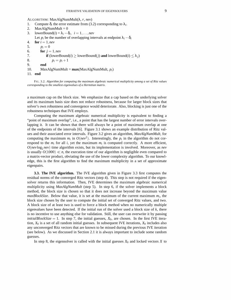
ALGORITHM: MaxAlgNumMult(λ, r, nev)1. Computeδi the error estimate from (3.2) corresponding toλi .2. MaxAlgNumMult = 03. lowerBound(i) = λi −δi , i = 1, . . . ,nev

Let pi be the number of overlapping intervals at endpointλi −δi

4. for i = 1,nev5. pi = 06. for j = 1,nev7. if (lowerBound(i) ≥ lowerBound(j) and lowerBound(i) ≤ λ j )8. pi = pi +19. end10. MaxAlgNumMult =max(MaxAlgNumMult, pi)11. end

FIG. 3.2. Algorithm for computing the maximum algebraic numerical multiplicity among a set of Ritz valuescorresponding to the smallest eigenvalues of a Hermitian matrix.

a maximum cap on the block size. We emphasize that a cap based on the underlying solverand its maximum basis size does not reduce robustness, because for larger block sizes thatsolver’s own robustness and convergence would deteriorate. Also, blocking is just one of therobustness techniques that IVE employs.

Computing the maximum algebraic numerical multiplicity isequivalent to finding a“point of maximum overlap”, i.e., a point that has the largest number of error intervals over-lapping it. It can be shown that there will always be a point ofmaximum overlap at oneof the endpoints of the intervals [6]. Figure 3.1 shows an example distribution of Ritz val-ues and their associated error intervals. Figure 3.2 gives an algorithm,MaxAlgNumMult, forcomputing the maximummi in O(nev2). Interestingly, thepi in the algorithm do not cor-respond to themi for all i, yet the maximummi is computed correctly. A more efficient,O(nevlog2nev) time algorithm exists, but its implementation is involved.Moreover, asnevis usuallyO(1000) � n, the execution time of our algorithm is negligible even compared toa matrix-vector product, obviating the use of the lower complexity algorithm. To our knowl-edge, this is the first algorithm to find the maximum multiplicity in a set of approximateeigenpairs.

3.3. The IVE algorithm. The IVE algorithm given in Figure 3.3 first computes theresidual norms of the converged Ritz vectors (step 4). This step is not required if the eigen-solver returns this information. Then, IVE determines the maximum algebraic numericalmultiplicity using MaxAlgNumMult(step 5). In step 6, if the solver implements a blockmethod, the block size is chosen so that it does not increase beyond the maximum valuemaxBlockSize. Below that value, it is set at the maximum of the current maximum mi , theblock size chosen by the user to compute the initial set of converged Ritz values, and two.A block size of at least two is used to force a block method whenno numerically multipleeigenvalues have been detected. If the initial run of the solver used a block size ofk, thereis no incentive to use anything else for validation. Still, the user can overwrite it by passinginitialBlockSize= 1. In step 7, the initial guesses,X0, are chosen. In the first IVE itera-tion, X0 is a set of all random initial guesses. In subsequent IVE iterations,X0 includes alsoany unconverged Ritz vectors that are known to be missed during the previous IVE iteration(see below). As we discussed in Section 2.1 it is always important to include some randomguesses.

In step 8, the eigensolver is called with the initial guessesX0 and locked vectorsX to


ALGORITHM: [X, λ] = IVE(A, X, λ, resNorms, initialBlockSize, maxBasisSize)Let X andλ be the converged Ritz vectors and Ritz values.Let initialBlockSize be the block size used to computeX.Let maxBlockSize be the maximum block size allowed1. numNew = 12. Xmissed= [ ], Xunconverged= [ ]3. repeat4. resNorms = ComputeResNorms(A, X, λ)5. newMult = MaxAlgNumMult(λ, resNorms)6. if (solver implements block)

blockSize =min(maxBlockSize,max(newMult, initialBlockSize, 2))else

blockSize = 17. X0 = [Xmissed, rand(blockSize -size(Xunconverged))]8. Compute[Xnew,λnew,Xunconverged,λunconverged] by calling the solver:

if (solver implements external locking)Solver(A, numNew,X0, X)

elseSolver((I −XXT)(A−σI), numNew,X0)

9. [X,λ] = InsertionSort(Xnew, λnew, numNew,X, λ, resNorms)l0. numMissedUnconv = NumMissedValues(λ, λunconverged, blockSize-numNew)11. Xmissed= Xunconverged(:,1:numMissedUnconv)12. numNew =max(1, numMissedUnconv)13. until (X did not changedand numMissedUnconv= 0 )

FIG. 3.3. IVE algorithm for computing missed eigenpairs. IVE is a wrapper around an existing Hermitian,Rayleigh-Ritz based eigensolver.

find numNewmore eigenpairs. Depending on the solver, external or explicit locking can beperformed. Note that the IVE algorithm assumes that the chosen solver returns not only thenumNewconverged Ritz values inλnew, but also the remainingblockSize−numNewuncon-verged Ritz values inλunconverged. Solvers that do not return the unconverged Ritz pairs bydefault can be easily modified to do so. Otherwise, we can setnumMissedUnconv= 0.

In step 9, an insertion sort (see Figure 3.4 for details) is called to insert any converged,missed eigenpairs inλnew andXnew into λ andX, respectively. For every missed Ritz valueinserted into theλ array, the largestλnev in the array and the corresponding vector inXare removed. If enough storage is available, those removed converged eigenvectors can stillremain in the locked array to avoid possible recomputation.We choose not to take advantageof this feature in our experiments. If none of the recently converged Ritz values were missed,then the IVE algorithm will terminate at step 13.

Step 10 calls the algorithmNumMissedValuesin Figure 3.5 to determine how many ofthe unconverged Ritz values inλunconvergedare missed values. A Ritz value inλunconvergedisconsidered missed if it is smaller thanλnev. Because of monotonic convergence, these Ritzvalues will only continue to decrease and approach missed eigenvalues. Therefore, it is wiseto use the corresponding unconverged Ritz vectors inXunconvergedas initial guesses (step 11).These can significantly reduce validation time when many eigenvalues are missed, becausethey enable the solver to avoid repeating convergence through random guesses.

Finally, step 12 sets the new number of Ritz values the solvermust compute. Clearly, weshould continue and find thenumMissedUnconvmissed ones that step 10 may have identified.


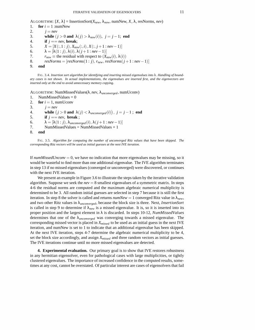
ALGORITHM: [X, λ] = InsertionSort(Xnew, λnew, numNew,X, λ, resNorms,nev)1. for i = 1 :numNew2. j = nev3. while ( j > 0 and λ( j) > λnew(i)), j = j −1; end4. if j == nev, break;5. X = [X(:,1 : j), Xnew(:, i), X(:, j +1 : nev−1)]6. λ = [λ(1 : j), λ(i), λ( j +1 : nev−1)]7. rnew≡ the residual with respect to(Xnew(i), λ(i))8. resNorms= [resNorms(1 : j), rnew, resNorms( j +1 : nev−1)]9. end

FIG. 3.4. Insertion sort algorithm for identifying and inserting missed eigenvalues intoλ. Handling of bound-ary cases is not shown. In actual implementations, the eigenvalues are inserted first, and the eigenvectors areinserted only at the end to avoid unnecessary memory copying.

ALGORITHM: NumMissedValues(λ,nev, λunconverged, numUconv)1. NumMissedValues = 02. for i = 1, numUconv3. j = nev4. while

(

j > 0 and λ( j) < λunconverged(i))

, j = j −1 ; end5. if j == nev, break ;6. λ = [λ(1 : j), λunconverged(i), λ( j +1 : nev−1)]7. NumMissedValues = NumMissedValues + 18. end

FIG. 3.5. Algorithm for computing the number of unconverged Ritz values that have been skipped. Thecorresponding Ritz vectors will be used as initial guesses at the next IVE iteration.

If numMissedUnconv= 0, we have no indication that more eigenvalues may be missing, so itwould be wasteful to find more than one additional eigenvalue. The IVE algorithm terminatesin step 13 if no missed eigenvalues (converged or unconverged) were discovered, or continueswith the next IVE iteration.

We present an example in Figure 3.6 to illustrate the steps taken by the iterative validationalgorithm. Suppose we seek thenev= 8 smallest eigenvalues of a symmetric matrix. In steps4-6 the residual norms are computed and the maximum algebraic numerical multiplicity isdetermined to be 3. All random initial guesses are selected in step 7 because it is still the firstiteration. In step 8 the solver is called and returnsnumNew= 1 converged Ritz value inλnew,and two other Ritz values inλunconverged, because the block size is three. Next,InsertionSortis called in step 9 to determine ifλnew is a missed eigenvalue. It is, so it is inserted into itsproper position and the largest element inλ is discarded. In steps 10-12,NumMissedValuesdetermines that one of theλunconvergedwas converging towards a missed eigenvalue. Thecorresponding missed vector is placed inXmissedto be used as an initial guess in the next IVEiteration, and numNew is set to 1 to indicate that an additional eigenvalue has been skipped.At the next IVE iteration, steps 4-7 determine the algebraicnumerical multiplicity to be 4,set the block size accordingly, and assignXmissedand three random vectors as initial guesses.The IVE iterations continue until no more missed eigenvalues are detected.

4. Experimental evaluation. Our primary goal is to show that IVE restores robustnessin any hermitian eigensolver, even for pathological cases with large multiplicities, or tightlyclustered eigenvalues. The importance of increased confidence in the computed results, some-times at any cost, cannot be overstated. Of particular interest are cases of eigensolvers that fail


Steps 4−6

newMult = 3]X = [

0

Locked

blockSize = 3

Step 7

λ unconvergedλnew

numNew = 1 2 = blockSize − numNewLocked

Step 8

λ new unconverged Discardedλ

Step 9

Locked

] = [Xmissed

numNew = 1

numMissedUnconv = 1

Steps 10−12

0

newMult = 4]

Locked

X = [blockSize = 4

Steps 4−7

of largest alg. num. mult.

Converged Converged, missedKey

Unconverged, not missed

Unconverged, missed

Random initial

newMult = 3blockSize = 3numNew = 1

Converged pair vector

Locked

FIG. 3.6.Example validation problem.

to find all the required eigenvalues, regardless of the initial choice of parameters, yet guidedby IVE, they succeed. A secondary goal is to demonstrate how IVE can decouple robustnessfrom performance, so that solvers are run with default settings for best performance and anymissed eigenpairs are obtained later in a shorter IVE cycle.

4.1. Eigensolvers used in the evaluation. We have used five different eigensolversfrom three eigensolver packages. The first is IRBL, the Implicitly Restarted Block Lanczosmethod [2, 1], which uses implicit restarting combined withLeja shifts to improve conver-gence of the standard Lanczos method. IRBL is a block method and implements both externaland internal locking. For our tests, we have added three lines of code in IRBL to allow it toreturn all Ritz pairs in the block, not only the converged ones. IRBL is implemented inMATLAB, and therefore it is used mainly to demonstrate the IVE benefits on robustness andconvergence; not on timings.

The second symmetric solver is the function dsaupd from the popular software packageARPACK [19]. Henceforth, we will refer to the particular eigensolver as ARPACK. ARPACKis based also on implicit restarting, but unlike IRBL, it uses the Ritz values as the restartingshifts. ARPACK is a single vector method and does not implement external or internal lock-ing. Thus, in a sense, it represents a worst case scenario, asIVE cannot employ all of itstechniques. In particular, IVE is restricted to usingblockSize= 1, numMissedUnconv= 0,and thusnumNew= 1, and locking must be implemented explicitly in IVE. No modificationswere made to the ARPACK code which is implemented in Fortran 77.

The remaining three solvers come from PRIMME, a software package that we have de-veloped in C, and which is freely available [20]. PRIMME, or PReconditioned Iterative Mul-


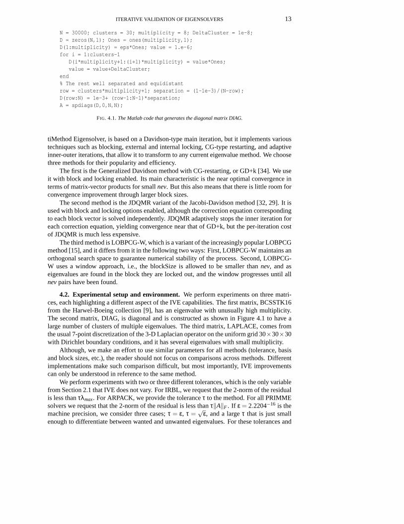
N = 30000; clusters = 30; multiplicity = 8; DeltaCluster = 1e-8;D = zeros(N,1); Ones = ones(multiplicity,1);D(1:multiplicity) = eps*Ones; value = 1.e-6;for i = 1:clusters-1

D(i*multiplicity+1:(i+1)*multiplicity) = value*Ones;value = value+DeltaCluster;

end% The rest well separated and equidistantrow = clusters*multiplicity+1; separation = (1-1e-3)/(N-row);D(row:N) = 1e-3+ (row-1:N-1)*separation;A = spdiags(D,0,N,N);

FIG. 4.1.The Matlab code that generates the diagonal matrix DIAG.

tiMethod Eigensolver, is based on a Davidson-type main iteration, but it implements varioustechniques such as blocking, external and internal locking, CG-type restarting, and adaptiveinner-outer iterations, that allow it to transform to any current eigenvalue method. We choosethree methods for their popularity and efficiency.

The first is the Generalized Davidson method with CG-restarting, or GD+k [34]. We useit with block and locking enabled. Its main characteristic is the near optimal convergence interms of matrix-vector products for smallnev. But this also means that there is little room forconvergence improvement through larger block sizes.

The second method is the JDQMR variant of the Jacobi-Davidson method [32, 29]. It isused with block and locking options enabled, although the correction equation correspondingto each block vector is solved independently. JDQMR adaptively stops the inner iteration foreach correction equation, yielding convergence near that of GD+k, but the per-iteration costof JDQMR is much less expensive.

The third method is LOBPCG-W, which is a variant of the increasingly popular LOBPCGmethod [15], and it differs from it in the following two ways:First, LOBPCG-W maintains anorthogonal search space to guarantee numerical stability of the process. Second, LOBPCG-W uses a window approach, i.e., the blockSize is allowed to besmaller thannev, and aseigenvalues are found in the block they are locked out, and the window progresses until allnevpairs have been found.

4.2. Experimental setup and environment. We perform experiments on three matri-ces, each highlighting a different aspect of the IVE capabilities. The first matrix, BCSSTK16from the Harwel-Boeing collection [9], has an eigenvalue with unusually high multiplicity.The second matrix, DIAG, is diagonal and is constructed as shown in Figure 4.1 to have alarge number of clusters of multiple eigenvalues. The thirdmatrix, LAPLACE, comes fromthe usual 7-point discretization of the 3-D Laplacian operator on the uniform grid 30×30×30with Dirichlet boundary conditions, and it has several eigenvalues with small multiplicity.

Although, we make an effort to use similar parameters for allmethods (tolerance, basisand block sizes, etc.), the reader should not focus on comparisons across methods. Differentimplementations make such comparison difficult, but most importantly, IVE improvementscan only be understood in reference to the same method.

We perform experiments with two or three different tolerances, which is the only variablefrom Section 2.1 that IVE does not vary. For IRBL, we request that the 2-norm of the residualis less thanτλmax. For ARPACK, we provide the toleranceτ to the method. For all PRIMMEsolvers we request that the 2-norm of the residual is less than τ‖A‖F . If ε = 2.2204−16 is themachine precision, we consider three cases;τ = ε, τ =

√ε, and a largeτ that is just small

enough to differentiate between wanted and unwanted eigenvalues. For these tolerances and


Table 4.1A: IRBL/BCSSTK16 Initial runsτ

k ε ε1/2 2.023e-51 57, 162390 28, 15728 21, 55142 68, 211526 32, 17616 23, 77063 74, 265125 32, 17844 23, 76654 73, 298884 32, 13748 24, 71685 74, 283880 32, 489830 24, 207006 74, 272868 38, 11340 20, 55627 74, 287693 29, 9541 21, 97238 74, 318568 32, 9560 19, 48969 74, 363123 36, 11007 23, 512110 74, 398170 32, 12890 20, 447015 74, 541230 39, 12600 22, 487520 74, 679760 56, 9140 37, 456074 74, 118696 74, 114848 74, 8362

Table 4.1B: IRBL/BCSSTK16 IVE runsτ

mxk ε ε1/2 2.023e-51 72992 6921 58282 97292 7821 60283 76223 9229 42864 59392 7721 36285 53892 6621 45286 41756 6745 36807 64478 6981 42448 40988 6937 39689 52166 7546 448410 58092 6121 4528

Best total MV for Initial + IVE run203378 21849 9142

k,mxk 1, 8 1, 10 1, 4TABLE 4.1

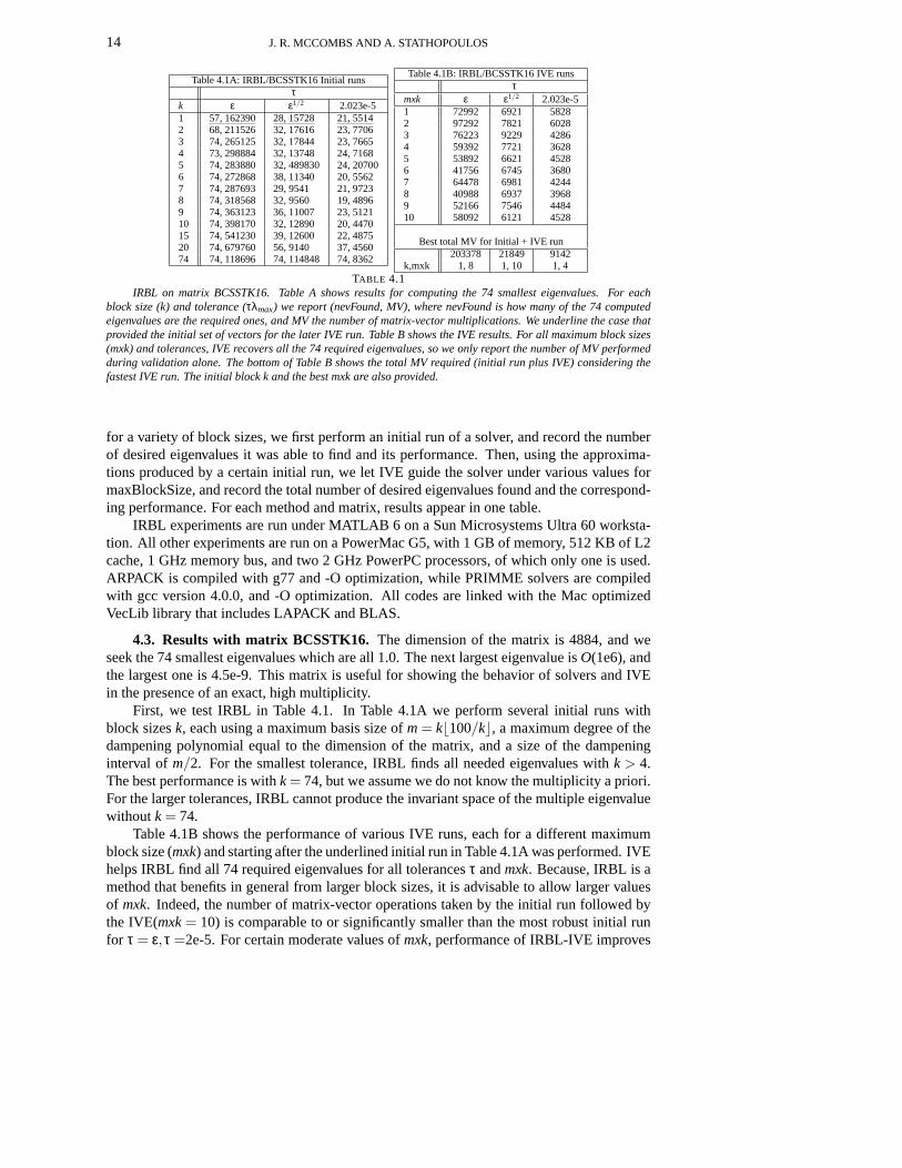
IRBL on matrix BCSSTK16. Table A shows results for computingthe 74 smallest eigenvalues. For eachblock size (k) and tolerance (τλmax) we report (nevFound, MV), where nevFound is how many of the 74 computedeigenvalues are the required ones, and MV the number of matrix-vector multiplications. We underline the case thatprovided the initial set of vectors for the later IVE run. Table B shows the IVE results. For all maximum block sizes(mxk) and tolerances, IVE recovers all the 74 required eigenvalues, so we only report the number of MV performedduring validation alone. The bottom of Table B shows the total MV required (initial run plus IVE) considering thefastest IVE run. The initial block k and the best mxk are also provided.

for a variety of block sizes, we first perform an initial run ofa solver, and record the numberof desired eigenvalues it was able to find and its performance. Then, using the approxima-tions produced by a certain initial run, we let IVE guide the solver under various values formaxBlockSize, and record the total number of desired eigenvalues found and the correspond-ing performance. For each method and matrix, results appearin one table.

IRBL experiments are run under MATLAB 6 on a Sun MicrosystemsUltra 60 worksta-tion. All other experiments are run on a PowerMac G5, with 1 GBof memory, 512 KB of L2cache, 1 GHz memory bus, and two 2 GHz PowerPC processors, of which only one is used.ARPACK is compiled with g77 and -O optimization, while PRIMME solvers are compiledwith gcc version 4.0.0, and -O optimization. All codes are linked with the Mac optimizedVecLib library that includes LAPACK and BLAS.

4.3. Results with matrix BCSSTK16. The dimension of the matrix is 4884, and weseek the 74 smallest eigenvalues which are all 1.0. The next largest eigenvalue isO(1e6), andthe largest one is 4.5e-9. This matrix is useful for showing the behavior of solvers and IVEin the presence of an exact, high multiplicity.

First, we test IRBL in Table 4.1. In Table 4.1A we perform several initial runs withblock sizesk, each using a maximum basis size ofm= kb100/kc, a maximum degree of thedampening polynomial equal to the dimension of the matrix, and a size of the dampeninginterval of m/2. For the smallest tolerance, IRBL finds all needed eigenvalues withk > 4.The best performance is withk = 74, but we assume we do not know the multiplicity a priori.For the larger tolerances, IRBL cannot produce the invariant space of the multiple eigenvaluewithout k = 74.

Table 4.1B shows the performance of various IVE runs, each for a different maximumblock size (mxk) and starting after the underlined initial run in Table 4.1Awas performed. IVEhelps IRBL find all 74 required eigenvalues for all tolerances τ andmxk. Because, IRBL is amethod that benefits in general from larger block sizes, it isadvisable to allow larger valuesof mxk. Indeed, the number of matrix-vector operations taken by the initial run followed bythe IVE(mxk= 10) is comparable to or significantly smaller than the most robust initial runfor τ = ε,τ =2e-5. For certain moderate values ofmxk, performance of IRBL-IVE improves


Table 4.2A: GD+k/BCSSTK16 Initial runsτ

k ε ε1/2 1e-61 37, 15097, 93 20, 5469, 37 13, 3232, 252 39, 16994, 97 24, 6883, 42 16, 4059, 273 41, 19591, 113 25, 7593, 46 17, 4510, 304 45, 20247, 121 27, 7700, 48 19, 4652, 305 49, 22214, 135 28, 7974, 50 20, 4968, 336 44, 28814, 168 27, 10640, 67 19, 6046, 407 54, 23754, 149 30, 8834, 56 22, 5451, 378 51, 25012, 155 29, 9761, 63 21, 5884, 399 48, 35213, 225 28, 12922, 85 21, 7476, 5310 74, 40940, 305 37, 9557, 72 27, 6167, 4715 74, 37138, 370 36, 8134, 83 32, 5181, 4920 74, 31794, 362 42, 9027, 104 26, 5018, 6030 73, 24647, 364 42, 7249, 102 30, 4609, 7140 74, 26451, 497 42, 7111, 135 42, 4473, 8750 74, 20936, 458 55, 7089, 165 52, 4789, 11174 74, 19058, 600 73, 6946, 220 71, 4575, 153

Table 4.2B: GD+k/BCSSTK16 IVE runsτ

mxk ε ε1/2 1e-61 9572, 82 5943, 45 4274, 332 9464, 77 6070, 42 4564, 323 8679, 69 6028, 41 4803, 334 9300, 77 6284, 45 4784, 345 9585, 78 6256, 47 5056, 386 9555, 78 5980, 45 5060, 367 11044, 95 6547, 49 4973, 388 15584, 152 6944, 52 4802, 35

Best total MV/times for Initial + IVE run28270, 182 11497, 78 7796, 57

k,mxk 3, 3 1, 3 1, 2

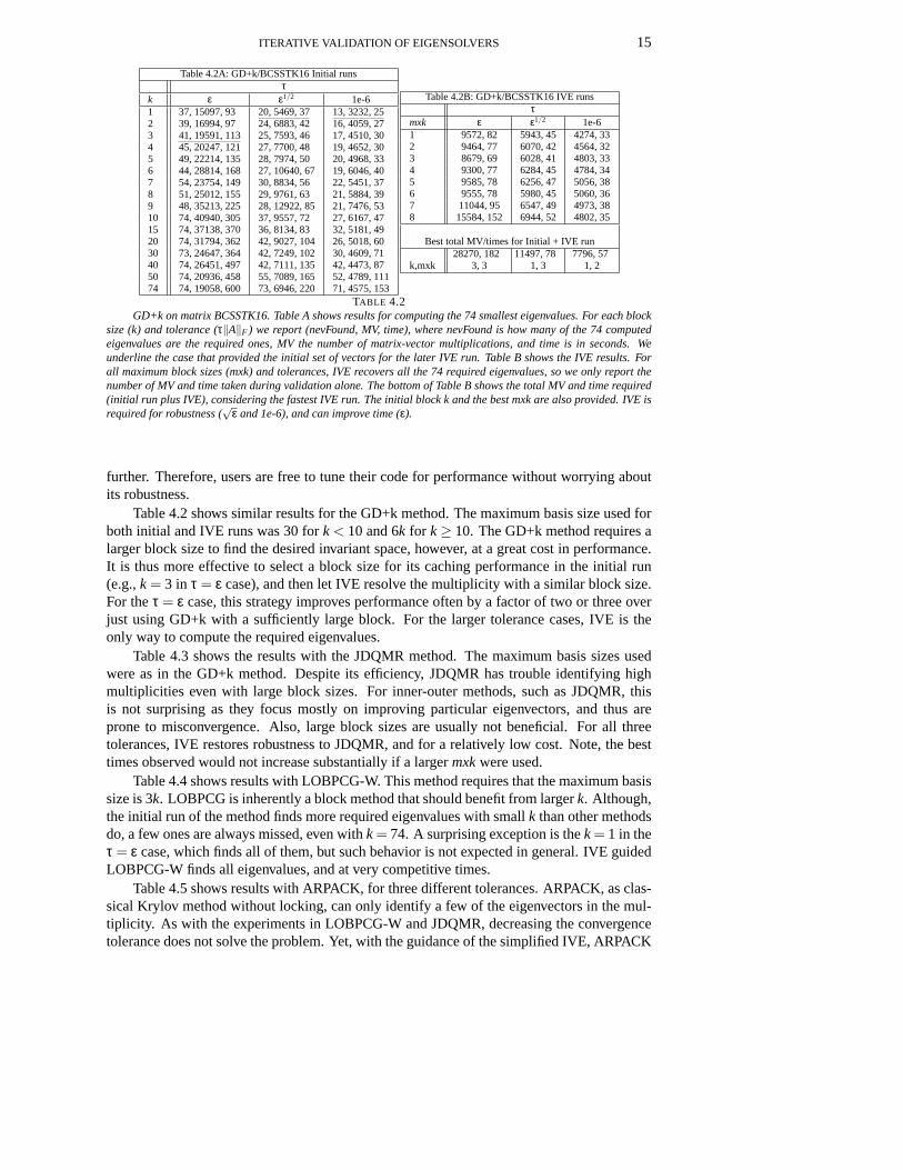
TABLE 4.2GD+k on matrix BCSSTK16. Table A shows results for computingthe 74 smallest eigenvalues. For each block

size (k) and tolerance (τ‖A‖F ) we report (nevFound, MV, time), where nevFound is how many of the 74 computedeigenvalues are the required ones, MV the number of matrix-vector multiplications, and time is in seconds. Weunderline the case that provided the initial set of vectors for the later IVE run. Table B shows the IVE results. Forall maximum block sizes (mxk) and tolerances, IVE recovers all the 74 required eigenvalues, so we only report thenumber of MV and time taken during validation alone. The bottom of Table B shows the total MV and time required(initial run plus IVE), considering the fastest IVE run. Theinitial block k and the best mxk are also provided. IVE isrequired for robustness (

√ε and 1e-6), and can improve time (ε).

further. Therefore, users are free to tune their code for performance without worrying aboutits robustness.

Table 4.2 shows similar results for the GD+k method. The maximum basis size used forboth initial and IVE runs was 30 fork < 10 and 6k for k≥ 10. The GD+k method requires alarger block size to find the desired invariant space, however, at a great cost in performance.It is thus more effective to select a block size for its caching performance in the initial run(e.g.,k = 3 in τ = ε case), and then let IVE resolve the multiplicity with a similar block size.For theτ = ε case, this strategy improves performance often by a factor of two or three overjust using GD+k with a sufficiently large block. For the larger tolerance cases, IVE is theonly way to compute the required eigenvalues.

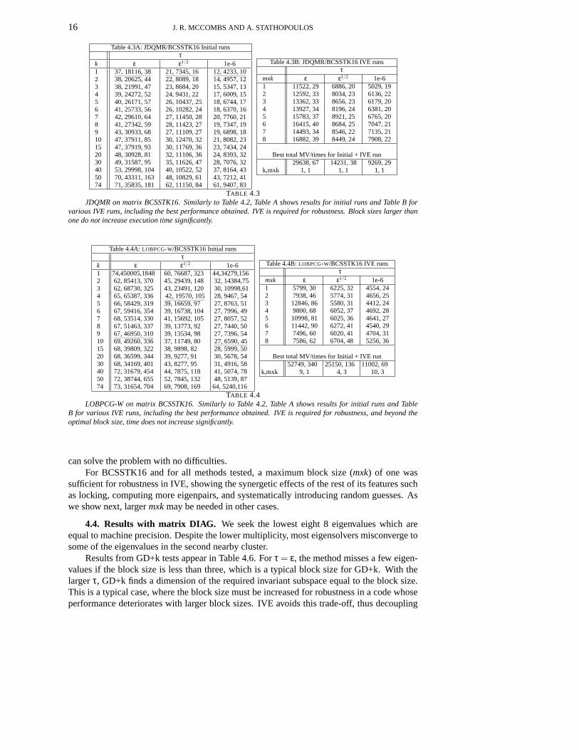
Table 4.3 shows the results with the JDQMR method. The maximum basis sizes usedwere as in the GD+k method. Despite its efficiency, JDQMR has trouble identifying highmultiplicities even with large block sizes. For inner-outer methods, such as JDQMR, thisis not surprising as they focus mostly on improving particular eigenvectors, and thus areprone to misconvergence. Also, large block sizes are usually not beneficial. For all threetolerances, IVE restores robustness to JDQMR, and for a relatively low cost. Note, the besttimes observed would not increase substantially if a largermxkwere used.

Table 4.4 shows results with LOBPCG-W. This method requiresthat the maximum basissize is 3k. LOBPCG is inherently a block method that should benefit fromlargerk. Although,the initial run of the method finds more required eigenvalueswith smallk than other methodsdo, a few ones are always missed, even withk = 74. A surprising exception is thek = 1 in theτ = ε case, which finds all of them, but such behavior is not expected in general. IVE guidedLOBPCG-W finds all eigenvalues, and at very competitive times.

Table 4.5 shows results with ARPACK, for three different tolerances. ARPACK, as clas-sical Krylov method without locking, can only identify a fewof the eigenvectors in the mul-tiplicity. As with the experiments in LOBPCG-W and JDQMR, decreasing the convergencetolerance does not solve the problem. Yet, with the guidanceof the simplified IVE, ARPACK


Table 4.3A: JDQMR/BCSSTK16 Initial runsτ

k ε ε1/2 1e-61 37, 18116, 38 21, 7345, 16 12, 4233, 102 38, 20625, 44 22, 8089, 18 14, 4957, 123 38, 21991, 47 23, 8684, 20 15, 5347, 134 39, 24272, 52 24, 9431, 22 17, 6009, 155 40, 26171, 57 26, 10437, 25 18, 6744, 176 41, 25733, 56 26, 10282, 24 18, 6370, 167 42, 29610, 64 27, 11450, 28 20, 7760, 218 41, 27342, 59 28, 11423, 27 19, 7347, 199 43, 30933, 68 27, 11109, 27 19, 6898, 1810 47, 37911, 85 30, 12470, 32 21, 8082, 2315 47, 37919, 93 30, 11769, 36 23, 7434, 2420 48, 30928, 81 32, 11106, 36 24, 8393, 3230 49, 31587, 95 35, 11626, 47 28, 7076, 3240 53, 29998, 104 40, 10522, 52 37, 8164, 4350 70, 43311, 163 48, 10829, 61 43, 7212, 4174 71, 35835, 181 62, 11150, 84 61, 9407, 83

Table 4.3B: JDQMR/BCSSTK16 IVE runsτ

mxk ε ε1/2 1e-61 11522, 29 6886, 20 5029, 192 12592, 33 8034, 23 6136, 223 13362, 33 8656, 23 6179, 204 13927, 34 8196, 24 6381, 205 15783, 37 8921, 25 6765, 206 16415, 40 8684, 25 7047, 217 14493, 34 8546, 22 7135, 218 16882, 39 8449, 24 7908, 22


k,mxk 1, 1 1, 1 1, 1

TABLE 4.3JDQMR on matrix BCSSTK16. Similarly to Table 4.2, Table A shows results for initial runs and Table B for

various IVE runs, including the best performance obtained.IVE is required for robustness. Block sizes larger thanone do not increase execution time significantly.

Table 4.4A:LOBPCG-W/BCSSTK16 Initial runsτ

k ε ε1/2 1e-61 74,450005,1848 60, 76687, 323 44,34279,1562 62, 85413, 370 45, 29439, 148 32, 14384,753 62, 68730, 325 43, 23491, 120 30, 10998,614 65, 65387, 336 42, 19570, 105 28, 9467, 545 66, 58429, 319 39, 16659, 97 27, 8763, 516 67, 59416, 354 39, 16738, 104 27, 7996, 497 68, 53514, 330 41, 15692, 105 27, 8057, 528 67, 51463, 337 39, 13773, 92 27, 7440, 509 67, 46950, 310 39, 13534, 98 27, 7396, 5410 69, 49260, 336 37, 11749, 80 27, 6590, 4515 68, 39809, 322 38, 9898, 82 28, 5999, 5020 68, 36599, 344 39, 9277, 91 30, 5678, 5430 68, 34169, 401 43, 8277, 95 31, 4916, 5840 72, 31679, 454 44, 7875, 118 41, 5074, 7850 72, 38744, 655 52, 7845, 132 48, 5139, 8774 73, 31654, 704 69, 7908, 169 64, 5240,116

Table 4.4B:LOBPCG-W/BCSSTK16 IVE runsτ

mxk ε ε1/2 1e-61 5799, 30 6225, 32 4554, 242 7938, 46 5774, 31 4656, 253 12846, 86 5580, 31 4412, 244 9800, 68 6052, 37 4692, 285 10998, 81 6025, 36 4641, 276 11442, 90 6272, 41 4540, 297 7496, 60 6020, 41 4704, 318 7586, 62 6704, 48 5256, 36


k,mxk 9, 1 4, 3 10, 3

TABLE 4.4LOBPCG-W on matrix BCSSTK16. Similarly to Table 4.2, Table Ashows results for initial runs and Table

B for various IVE runs, including the best performance obtained. IVE is required for robustness, and beyond theoptimal block size, time does not increase significantly.

can solve the problem with no difficulties.For BCSSTK16 and for all methods tested, a maximum block size(mxk) of one was

sufficient for robustness in IVE, showing the synergetic effects of the rest of its features suchas locking, computing more eigenpairs, and systematicallyintroducing random guesses. Aswe show next, largermxkmay be needed in other cases.

4.4. Results with matrix DIAG. We seek the lowest eight 8 eigenvalues which areequal to machine precision. Despite the lower multiplicity, most eigensolvers misconverge tosome of the eigenvalues in the second nearby cluster.

Results from GD+k tests appear in Table 4.6. Forτ = ε, the method misses a few eigen-values if the block size is less than three, which is a typicalblock size for GD+k. With thelargerτ, GD+k finds a dimension of the required invariant subspace equal to the block size.This is a typical case, where the block size must be increasedfor robustness in a code whoseperformance deteriorates with larger block sizes. IVE avoids this trade-off, thus decoupling


Table 4.5 ARPACK/BCSSTK16Initial runs IVE run

τ evals MV Time evals Total MV Total time1e-16 29 4435 86 74 20567 2591e-8 6 1240 20 74 18233 2261e-7 5 1150 18 74 16974 211

TABLE 4.5ARPACK on matrix BCSSTK16. This is not a block method, so we only vary the toleranceτ. We report

(nevFound, MV, time) for the initial run of ARPACK, and the total (nevFound, MV, time) taken by both initial and thesubsequent IVE runs. The robustness gains are significant.

Table 4.6A: GD+k/DIAG Initial runsτ

k ε 5ε1/2

1 5, 6777, 178.1 1, 567, 14.92 6, 13118, 305.4 2, 564, 11.63 8, 203927, 5127.2 3, 1267, 28.74 8, 24124, 521.0 4, 1548, 31.15 8, 48110, 1147.3 5, 2230, 50.16 8, 43310, 1056.9 6, 2401, 55.17 8, 86573, 2142.4 7, 4376, 105.08 8, 88696, 2264.9 8, 7008, 168.1

Table 4.6B: GD+k/DIAG IVE runsτ

mxk ε 5ε1/2

1 8, 3858, 89.1 4, 598, 13.22 8, 7184, 162.0 6, 976, 19.53 8, 8337, 159.6 8, 1480, 29.14 8, 34628, 770.1 8, 2216, 44.65 8, 47253, 1014.4 8, 2300, 39.96 8, 508381, 11340.8 8, 3159, 59.27 8, >600K 13384.4 8, 3827, 76.98 8, >600K 16084.9 8, 3532, 78.5

Best total MV/times for Initial + IVE run10635, 267.2 2044, 40.7

k,mxk 1, 1 2, 3TABLE 4.6

GD+k on matrix DIAG. Table A shows results for computing the 8smallest eigenvalues, and Table B showsthe subsequent IVE results. We follow the same format as in previous tables, reporting (nevFound, MV, time) for theinitial as well as the IVE runs. A higher block size is needed in caseτ = 5

√ε to find all the desired eigenvalues.

Although GD+k does not benefit from large block size in general, performance improves through an efficient initialrun followed by a robust IVE run.

performance and robustness. By choosing anmxksuch as 2 or 3, which is reasonable for lowtolerances in GD+k (and not depending on the particular problem), IVE helps GD+k find allrequired eigenvalues and much faster than any initial run byGD+k. As expected, a slightlylarger block may be needed for larger tolerances, but its exact value does not significantlyaffect performance. Note that forτ = 5ε1/2, IVE must be allowed to set a block size largerthan one to recover robustness.

In Table 4.7 we show results from JDQMR on the DIAG matrix. As with GD+k, IVEcan recover robustness for JDQMR if it is allowed to use a larger block size. Moreover,mxkdoes not have to match the multiplicity sought (as is necessary in the initial runs), because thesynergy of the many IVE features compensates for smaller block sizes. For this solver, IVEexecution times are relatively insensitive tomxk, matching the best performance of the initialruns and with the added robustness.

In Table 4.8, LOBPCG-W finds all the required eigenvalues forτ = ε and for allk, exceptfor k = 2 for which IVE recovers the missing eigenvalue for a relatively small additional cost.Surprisingly, forτ = 5ε1/2 LOBPCG-W cannot identify the full invariant subspace in theinitial run, regardless of block size. When IVE is allowed to increase the block size abovethree, all eigenvalues are found.

Finally, in Table 4.9, we show the results from ARPACK on the DIAG matrix and forthree different tolerances. Through a combination of locking, restarting and finding moreeigenvalues IVE is able to recover all needed eigenvalues, except whenτ = 1e−7 which isclose to the first intercluster gap. As with the rest of the methods, a slightly larger block sizewould have resolved the problems.

Up to now, we have seen test cases where keepingmxk= 1 achieved both the required


Table 4.7A: JDQMR/DIAG Initial runsτ

k ε 5ε1/2

1 5, 7412, 21.5 1, 776, 4.52 6, 9382, 29.1 2, 765, 4.23 7, 12230, 38.5 3, 1453, 6.94 8, 12998, 38.8 4, 1650, 7.65 8, 14537, 47.7 5, 1401, 6.36 8, 16583, 52.7 6, 1648, 7.47 8, 17990, 61.4 7, 2822, 12.78 8, 11402, 36.7 8, 3908, 17.4

Table 4.7B: JDQMR/DIAG IVE runsτ

mxk ε 5ε1/2

1 8, 4471, 13.6 1, 406, 2.32 8, 7967, 25.6 1, 1462, 8.43 8, 11723, 33.8 6, 1855, 8.44 8, 18817, 57.2 8, 3229, 15.25 8, 25618, 77.9 6, 2597, 11.06 8, 33243, 99.8 8, 3950, 18.47 8, 35727, 108.7 8, 4431, 19.68 8, 39984, 118.1 8, 3592, 17.8


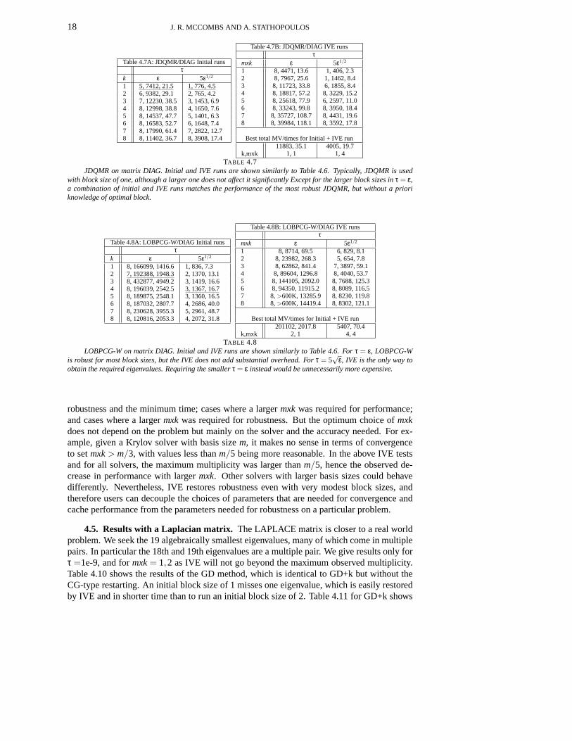
k,mxk 1, 1 1, 4TABLE 4.7

JDQMR on matrix DIAG. Initial and IVE runs are shown similarly to Table 4.6. Typically, JDQMR is usedwith block size of one, although a larger one does not affect it significantly Except for the larger block sizes inτ = ε,a combination of initial and IVE runs matches the performance of the most robust JDQMR, but without a prioriknowledge of optimal block.

Table 4.8A: LOBPCG-W/DIAG Initial runsτ

k ε 5ε1/2

1 8, 166099, 1416.6 1, 836, 7.32 7, 192388, 1948.3 2, 1370, 13.13 8, 432877, 4949.2 3, 1419, 16.64 8, 196039, 2542.5 3, 1367, 16.75 8, 189875, 2548.1 3, 1360, 16.56 8, 187032, 2807.7 4, 2686, 40.07 8, 230628, 3955.3 5, 2961, 48.78 8, 120816, 2053.3 4, 2072, 31.8

Table 4.8B: LOBPCG-W/DIAG IVE runsτ

mxk ε 5ε1/2

1 8, 8714, 69.5 6, 829, 8.12 8, 23982, 268.3 5, 654, 7.83 8, 62862, 841.4 7, 3897, 59.14 8, 89604, 1296.8 8, 4040, 53.75 8, 144105, 2092.0 8, 7688, 125.36 8, 94350, 11915.2 8, 8089, 116.57 8, >600K, 13285.9 8, 8230, 119.88 8, >600K, 14419.4 8, 8302, 121.1


k,mxk 2, 1 4, 4TABLE 4.8

LOBPCG-W on matrix DIAG. Initial and IVE runs are shown similarly to Table 4.6. Forτ = ε, LOBPCG-Wis robust for most block sizes, but the IVE does not add substantial overhead. Forτ = 5

√ε, IVE is the only way to

obtain the required eigenvalues. Requiring the smallerτ = ε instead would be unnecessarily more expensive.

robustness and the minimum time; cases where a largermxkwas required for performance;and cases where a largermxkwas required for robustness. But the optimum choice ofmxkdoes not depend on the problem but mainly on the solver and theaccuracy needed. For ex-ample, given a Krylov solver with basis sizem, it makes no sense in terms of convergenceto setmxk> m/3, with values less thanm/5 being more reasonable. In the above IVE testsand for all solvers, the maximum multiplicity was larger than m/5, hence the observed de-crease in performance with largermxk. Other solvers with larger basis sizes could behavedifferently. Nevertheless, IVE restores robustness even with very modest block sizes, andtherefore users can decouple the choices of parameters thatare needed for convergence andcache performance from the parameters needed for robustness on a particular problem.

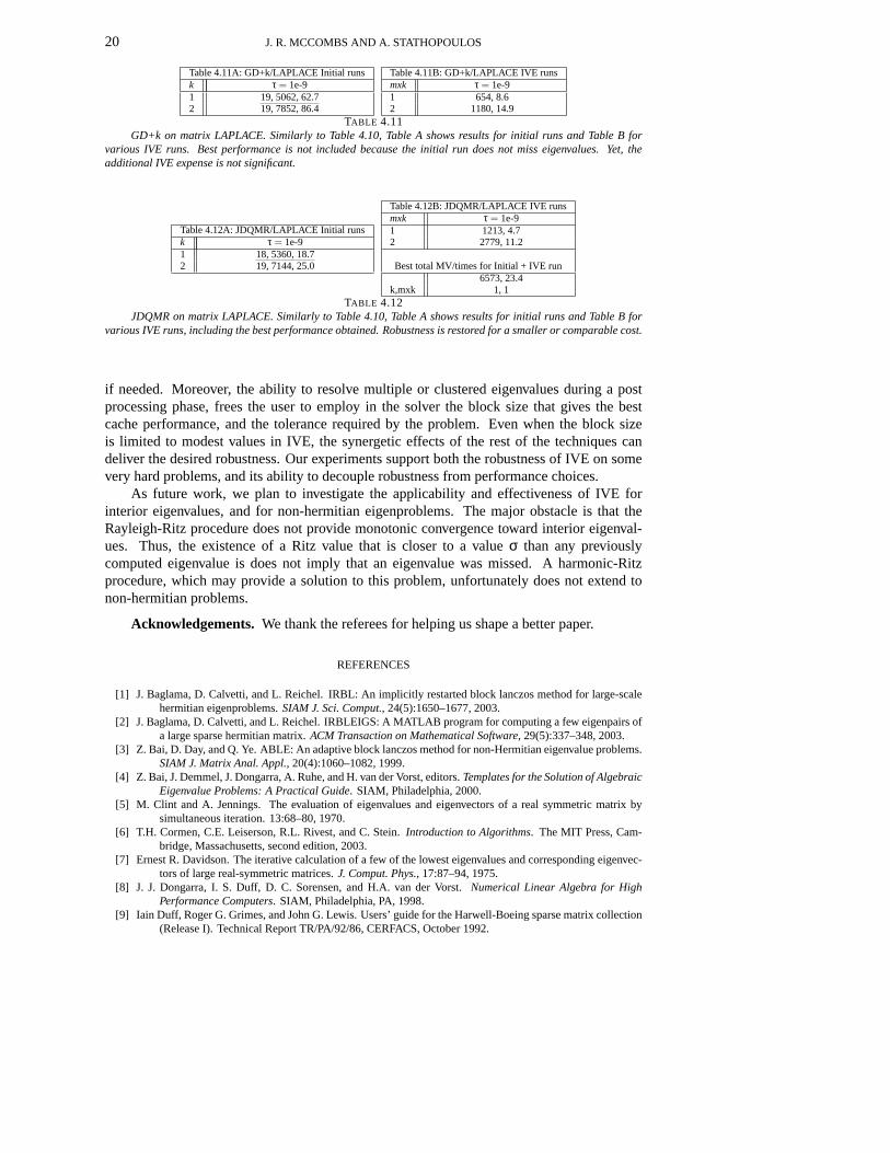
4.5. Results with a Laplacian matrix. The LAPLACE matrix is closer to a real worldproblem. We seek the 19 algebraically smallest eigenvalues, many of which come in multiplepairs. In particular the 18th and 19th eigenvalues are a multiple pair. We give results only forτ =1e-9, and formxk= 1,2 as IVE will not go beyond the maximum observed multiplicity.Table 4.10 shows the results of the GD method, which is identical to GD+k but without theCG-type restarting. An initial block size of 1 misses one eigenvalue, which is easily restoredby IVE and in shorter time than to run an initial block size of 2. Table 4.11 for GD+k shows


Table 4.9 ARPACK/DIAGInitial runs IVE run

τ evals MV Time evals Total MV Total time1e-16 5 305990 5004 8 309889 50921e-8 5 27678 443 8 30885 5151e-7 2 4167 68 2 4256 70

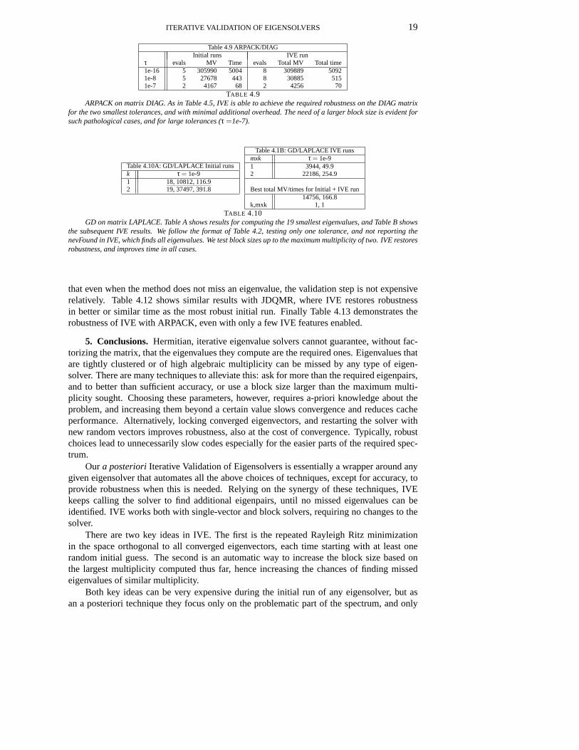
TABLE 4.9ARPACK on matrix DIAG. As in Table 4.5, IVE is able to achieve the required robustness on the DIAG matrix

for the two smallest tolerances, and with minimal additional overhead. The need of a larger block size is evident forsuch pathological cases, and for large tolerances (τ =1e-7).

Table 4.10A: GD/LAPLACE Initial runsk τ = 1e-91 18, 10812, 116.92 19, 37497, 391.8

Table 4.1B: GD/LAPLACE IVE runsmxk τ = 1e-91 3944, 49.92 22186, 254.9

Best total MV/times for Initial + IVE run14756, 166.8

k,mxk 1, 1TABLE 4.10

GD on matrix LAPLACE. Table A shows results for computing the19 smallest eigenvalues, and Table B showsthe subsequent IVE results. We follow the format of Table 4.2, testing only one tolerance, and not reporting thenevFound in IVE, which finds all eigenvalues. We test block sizes up to the maximum multiplicity of two. IVE restoresrobustness, and improves time in all cases.

that even when the method does not miss an eigenvalue, the validation step is not expensiverelatively. Table 4.12 shows similar results with JDQMR, where IVE restores robustnessin better or similar time as the most robust initial run. Finally Table 4.13 demonstrates therobustness of IVE with ARPACK, even with only a few IVE features enabled.

5. Conclusions. Hermitian, iterative eigenvalue solvers cannot guarantee, without fac-torizing the matrix, that the eigenvalues they compute are the required ones. Eigenvalues thatare tightly clustered or of high algebraic multiplicity canbe missed by any type of eigen-solver. There are many techniques to alleviate this: ask formore than the required eigenpairs,and to better than sufficient accuracy, or use a block size larger than the maximum multi-plicity sought. Choosing these parameters, however, requires a-priori knowledge about theproblem, and increasing them beyond a certain value slows convergence and reduces cacheperformance. Alternatively, locking converged eigenvectors, and restarting the solver withnew random vectors improves robustness, also at the cost of convergence. Typically, robustchoices lead to unnecessarily slow codes especially for theeasier parts of the required spec-trum.

Our a posterioriIterative Validation of Eigensolvers is essentially a wrapper around anygiven eigensolver that automates all the above choices of techniques, except for accuracy, toprovide robustness when this is needed. Relying on the synergy of these techniques, IVEkeeps calling the solver to find additional eigenpairs, until no missed eigenvalues can beidentified. IVE works both with single-vector and block solvers, requiring no changes to thesolver.

There are two key ideas in IVE. The first is the repeated Rayleigh Ritz minimizationin the space orthogonal to all converged eigenvectors, eachtime starting with at least onerandom initial guess. The second is an automatic way to increase the block size based onthe largest multiplicity computed thus far, hence increasing the chances of finding missedeigenvalues of similar multiplicity.

Both key ideas can be very expensive during the initial run ofany eigensolver, but asan a posteriori technique they focus only on the problematicpart of the spectrum, and only


Table 4.11A: GD+k/LAPLACE Initial runsk τ = 1e-91 19, 5062, 62.72 19, 7852, 86.4

Table 4.11B: GD+k/LAPLACE IVE runsmxk τ = 1e-91 654, 8.62 1180, 14.9

TABLE 4.11GD+k on matrix LAPLACE. Similarly to Table 4.10, Table A shows results for initial runs and Table B for

various IVE runs. Best performance is not included because the initial run does not miss eigenvalues. Yet, theadditional IVE expense is not significant.

Table 4.12A: JDQMR/LAPLACE Initial runsk τ = 1e-91 18, 5360, 18.72 19, 7144, 25.0

Table 4.12B: JDQMR/LAPLACE IVE runsmxk τ = 1e-91 1213, 4.72 2779, 11.2

Best total MV/times for Initial + IVE run6573, 23.4

k,mxk 1, 1TABLE 4.12

JDQMR on matrix LAPLACE. Similarly to Table 4.10, Table A shows results for initial runs and Table B forvarious IVE runs, including the best performance obtained.Robustness is restored for a smaller or comparable cost.

if needed. Moreover, the ability to resolve multiple or clustered eigenvalues during a postprocessing phase, frees the user to employ in the solver the block size that gives the bestcache performance, and the tolerance required by the problem. Even when the block sizeis limited to modest values in IVE, the synergetic effects ofthe rest of the techniques candeliver the desired robustness. Our experiments support both the robustness of IVE on somevery hard problems, and its ability to decouple robustness from performance choices.

As future work, we plan to investigate the applicability andeffectiveness of IVE forinterior eigenvalues, and for non-hermitian eigenproblems. The major obstacle is that theRayleigh-Ritz procedure does not provide monotonic convergence toward interior eigenval-ues. Thus, the existence of a Ritz value that is closer to a value σ than any previouslycomputed eigenvalue is does not imply that an eigenvalue wasmissed. A harmonic-Ritzprocedure, which may provide a solution to this problem, unfortunately does not extend tonon-hermitian problems.

Acknowledgements. We thank the referees for helping us shape a better paper.

REFERENCES

[1] J. Baglama, D. Calvetti, and L. Reichel. IRBL: An implicitly restarted block lanczos method for large-scalehermitian eigenproblems.SIAM J. Sci. Comput., 24(5):1650–1677, 2003.

[2] J. Baglama, D. Calvetti, and L. Reichel. IRBLEIGS: A MATLAB program for computing a few eigenpairs ofa large sparse hermitian matrix.ACM Transaction on Mathematical Software, 29(5):337–348, 2003.

[3] Z. Bai, D. Day, and Q. Ye. ABLE: An adaptive block lanczos method for non-Hermitian eigenvalue problems.SIAM J. Matrix Anal. Appl., 20(4):1060–1082, 1999.

[4] Z. Bai, J. Demmel, J. Dongarra, A. Ruhe, and H. van der Vorst,editors.Templates for the Solution of AlgebraicEigenvalue Problems: A Practical Guide. SIAM, Philadelphia, 2000.

[5] M. Clint and A. Jennings. The evaluation of eigenvalues and eigenvectors of a real symmetric matrix bysimultaneous iteration. 13:68–80, 1970.

[6] T.H. Cormen, C.E. Leiserson, R.L. Rivest, and C. Stein.Introduction to Algorithms. The MIT Press, Cam-bridge, Massachusetts, second edition, 2003.

[7] Ernest R. Davidson. The iterative calculation of a few ofthe lowest eigenvalues and corresponding eigenvec-tors of large real-symmetric matrices.J. Comput. Phys., 17:87–94, 1975.

[8] J. J. Dongarra, I. S. Duff, D. C. Sorensen, and H.A. van derVorst. Numerical Linear Algebra for HighPerformance Computers. SIAM, Philadelphia, PA, 1998.

[9] Iain Duff, Roger G. Grimes, and John G. Lewis. Users’ guidefor the Harwell-Boeing sparse matrix collection(Release I). Technical Report TR/PA/92/86, CERFACS, October 1992.


Table 4.1 ARPACK/LAPLACEInitial runs IVE run

τ evals MV Time evals Total MV Total time1e-9 16 2874 72 19 6042 137

TABLE 4.13ARPACK on matrix DIAG. As in Table 4.5, IVE is able to achieve the required robustness on the LAPLACE

matrix. Note that ARPACK missed 3 eigenvalues despite a relatively low tolerance.

[10] Roman Geus.The Jacobi-Davidson algorithm for solving large sparse symmetric eigenvalue problems withapplication to the design of accelerator cavities. PhD thesis, ETH, 2002. Thesis. No. 14734.

[11] G. H. Golub and C. F. Van Loan.Matrix Computations. The John Hopkins University Press, Baltimore, MD21211, 1989.

[12] G. H. Golub and R. Underwood. The block Lanczos method forcomputing eigenvalues. In J. R. Rice, editor,Mathematical Software III, pages 361–377, New York, 1977. Academic Press.

[13] R. G. Grimes, J. G. Lewis, and H. D. Simon. A shifted block Lanczos algorithm for solving sparse symmetricgeneralized eigenproblems.SIAM J. Matrix Anal. Appl., 15(1):228–272, 1994.

[14] Christopher Hsu and James Demmel. Effects of block size on the block Lanczos algorithm. Technical report,Department of Mathematics, U.C. Berkeley, June, 2003.

[15] A. V. Knyazev. Toward the optimal preconditioned eigensolver: Locally Optimal Block Preconditioned Con-jugate Gradient method.SIAM J. Sci. Comput., 23(2):517–541, 2001.

[16] Arno B. J. Kuijlaars. Convergence analysis of krylov subspace iterations with methods from potential theory.SIAM Review, 48:3–40, 2006.

[17] C. Lanczos. An iterative method for the solution of the eigenvalue problem of linear differential and integraloperators.J. Res. Nat. Nur. Stand., 45:255–282, 1950.

[18] R. B. Lehoucq and D. C. Sorensen. Deflation techniques for an implicitly restarted arnoldi iteration.SIAM J.Matrix Anal. Appl., 17(4):789–821, 1996.

[19] R. B. Lehoucq, D. C. Sorensen, and C. Yang.ARPACK USERS GUIDE: Solution of Large Scale EigenvalueProblems with Implicitly Restarted Arnoldi Methods. SIAM, Philadelphia, PA, 1998.

[20] J. R. McCombs and A. Stathopoulos. Technical report.[21] R. B. Morgan. A harmonic restarted Arnoldi algorithm forcalculating eigenvalues and determining multiplic-

ity. LAA, to appear.[22] R. B. Morgan. On restarting the Arnoldi method for large nonsymmetric eigenvalue problems.Math. Comput.,

65:1213–1230, 1996.[23] R. B. Morgan and D. S. Scott. Generalizations of Davidson’s method for computing eigenvalues of sparse

symmetric matrices.SIAM J. Sci. Comput., 7:817–825, 1986.[24] Beresford N. Parlett.The Symmetric Eigenvalue Problem. SIAM, Philadelphia, PA, 1998.[25] Heinz Ruthishauser. Simultaneous iteration method for symmetric matrices.Numer. Math., 16:205–223,

1970.[26] Yousef Saad. On the rate of convergence of the Lanczos and the block-Lanczos methods.SIAM J. Numer.

Anal., 17:687–706, 1980.[27] Yousef Saad.Numerical methods for large eigenvalue problems. Manchester University Press, 1992.[28] G. L. G. Sleijpen, A. G. L. Booten, D. R. Fokkema, and H. A. van der Vorst. Jacobi-davidson type methods

for generalized eigenproblems and polynomial eigenproblems.BIT, 36(3):595–633, 1996.[29] G. L. G. Sleijpen and H. A. van der Vorst. A Jacobi-Davidson iteration method for linear eigenvalue problems.

SIAM J. Matrix Anal. Appl., 17(2):401–425, 1996.[30] D. C. Sorensen. Implicit application of polynomial filters in a K-step Arnoldi method.SIAM J. Matrix Anal.

Appl., 13(1):357–385, 1992.[31] D. C. Sorensen. Deflation for implicitly restarted Arnoldi methods. Technical Report Tech. Rep. TR98-12,

Department of Computational and Applied Mathematics, Rice University, 1998.[32] A. Stathopoulos. Nearly optimal preconditioned methodsfor hermitian eigenproblems under limited memory.

Part i: Seeking one eigenvalue. Technical Report Tech. report WM-CS-2005-03.[33] A. Stathopoulos and C. F. Fischer. A Davidson program for finding a few selected extreme eigenpairs of a

large, sparse, real, symmetric matrix.Computer Physics Communications, 79(2):268–290, 1994.[34] A. Stathopoulos and Y. Saad. Restarting techniques for(Jacobi-)Davidson symmetric eigenvalue methods.

Electr. Trans. Numer. Alg., 7:163–181, 1998.[35] A. Stathopoulos, Y. Saad, and K. Wu. Dynamic thick restarting of the Davidson, and the implicitly restarted

Arnoldi methods.SIAM J. Sci. Comput., 19(1):227–245, 1998.[36] W. J. Stewart and A. Jennings. ALGORITHM 570: LOPSI a simultaneous iteration method for real matrices.

ACM Transactions on Mathematical Software, 7(2):230–232, 1981.[37] Tianruo Yang. Theoretical error bounds on the convergence of the Lanczos and block-Lanczos methods.

Computers and Mathematics with Applications, 38:19–38, 1999.

Iterative Validation of Eigensolvers: A Scheme for Improving the Reliability of Hermitian Eigenvalue Solvers

Documents