A map of contour integral-based eigensolvers for solving ... · A map of contour integral-based eigensolvers for solving generalized eigenvalue problems Akira Imakura1,*, Lei Du2,

arX

iv:1

510.

0257

2v2

[mat

h.N

A]

9 N

ov 2

016

A map of contour integral-based eigensolvers forsolving generalized eigenvalue problems

Akira Imakura1,*, Lei Du2, and Tetsuya Sakurai1,3

1University of Tsukuba, Japan2Dalian University of Technology, China.

3JST/CREST

∗Email : [email protected]

Abstract

Recently, contour integral-based methods have been actively studied for solving in-terior eigenvalue problems that find all eigenvalues located in a certain region and theircorresponding eigenvectors. In this paper, we reconsider the algorithms of the five typ-ical contour integral-based eigensolvers from the viewpoint of projection methods, andthen map the relationships among these methods. From the analysis, we conclude thatall contour integral-based eigensolvers can be regarded asprojection methods and canbe categorized based on their subspace used, the type of projection and the problem towhich they are applied implicitly.

1 Introduction

In this paper, we consider computing all eigenvalues located in a certain region of a general-ized eigenvalue problem and their corresponding eigenvectors:

Axi = λiBxi, xi ∈ Cn \ 0, λi ∈ Ω ⊂ C, (1)

whereA,B ∈ Cn×n andzB −A are assumed as nonsingular for anyz on the boundaryΓ ofthe regionΩ. Let m be the number of target eigenvaluesλi ∈ Ω (counting multiplicity) andXΩ = [xi|λi ∈ Ω] be a matrix whose columns are the target eigenvectors.

In 2003, Sakurai and Sugiura proposed a powerful algorithm for solving the interioreigenvalue problem (1) [19]. Their projection-type methoduses certain complex momentmatrices constructed by a contour integral. The basic concept is to introduce the rationalfunction

r(z) := vH(zB −A)−1Bv, v, v ∈ Cn \ 0, (2)

whose poles are the eigenvalues of the generalized eigenvalue problem:Axi = λiBxi, andthen compute all poles located inΩ by Kravanja’s algorithm [16], which is based on Cauchy’sintegral formula.

Kravanja’s algorithm can be expressed as follows. LetΓ be a positively oriented Jordancurve, i.e., the boundary ofΩ. We define complex momentsµk as

µk :=1

2πi

∮

Γ

zkr(z)dz, k = 0, 1, . . . , 2M − 1.

Then, all poles located inΩ of a meromorphic functionr(z) are the eigenvalues of the gener-alized eigenvalue problem

H<Myi = θiHMyi, (3)

whereHM , H<M are Hankel matrices:

HM :=

µ0 µ1 · · · µM−1

µ1 µ2 · · · µM

......

. . ....

µM−1 µM · · · µ2M−2

, H<

M :=

µ1 µ2 · · · µM

µ2 µ3 · · · µM+1...

.... . .

...µM µM+1 · · · µ2M−1

.

Applying Kravanja’s algorithm to the rational function (2), the generalized eigenvalue prob-lem (1) reduces to the generalized eigenvalue problem with the Hankel matrices (3). Thisalgorithm is called the SS–Hankel method.

The SS–Hankel method has since been developed by several researchers. The SS–RRmethod based on the Rayleigh–Ritz procedure increases the accuracy of the eigenpairs [20].Block variants of the SS–Hankel and SS–RR methods (known as the block SS–Hankel and theblock SS–RR methods, respectively) improve stability of the algorithms [10–12]. The blockSS–Arnoldi method based on the block Arnoldi method has alsobeen proposed [13]. Differ-ent from these methods, Polizzi proposed the FEAST eigensolver for Hermitian generalizedeigenvalue problems, which is based on an accelerated subspace iteration with the Rayleigh–Ritz procedure [17]. Their original 2009 version has been further developed [9,23,24].

Meanwhile, the contour integral-based methods have been extended to nonlinear eigen-value problems. Nonlinear eigensolvers are based on the block SS–Hankel [1,2] and the blockSS–RR [25] methods and a different type of contour integral-based nonlinear eigensolver wasproposed by Beyn [6], which we call the Beyn method. More recently, an improvement ofthe Beyn method was proposed based on using the canonical polyadic decomposition [5].

For Hermitian case, i.e.,A is a Hermitian andB is a Hermitian positive definite, there areseveral related works based on Chebyshev polynomial filtering [7, 26] and based on rationalinterpolation [4]. Specifically, Austin et al. analyzed that the contour integral-based eigen-solvers have strong relationship with rational interpolation established in [3], and proposed aprojection type method only with real poles [4].

In this paper, we reconsider the algorithms of typical contour integral-based eigensolversof (1), namely, the block SS–Hankel method [10, 11], the block SS–RR method [12], theFEAST eigensolver [17], the block SS–Arnoldi method [13] and the Beyn method [6] asprojection methods. We then analyze and map the relationships among these methods. Fromthe map of the relationships, we also provide error analysesof each method. Here, we notethat our analyses cover the case of Jordan blocks of the size larger than one and infiniteeigenvalues (or even both).

The remainder of this paper is organized as follows. Sections 2 and 3 briefly describe thealgorithms of the contour integral-based eigensolvers andanalyze the properties of their typ-ical matrices, respectively. The relationships among these methods are analyzed and mappedin Section 4. Error analyses of the methods are presented in Section 5, and numerical experi-ments are conducted in Section 6. The paper concludes with Section 7.

Throughout, the following notations are used. LetV = [v1, v2, . . . , vL] ∈ Cn×L anddefine the range space of the matrixV by R(V ) := spanv1, v2, . . . , vL. In addition, for

2

A ∈ Cn×n, K

k (A, V ) andB

k (A, V ) are the block Krylov subspaces:

K

k (A, V ) := R([V,AV,A2V, . . . , Ak−1V ]),

B

k (A, V ) :=

k−1∑

i=0

AiV αi

∣∣∣∣∣αi ∈ CL×L

.

We also define a block diagonal matrix with block elementsDi ∈ Cni×ni constructed asfollows:

d⊕

i=1

Di = D1 ⊕D2 ⊕ · · · ⊕Dd =

D1

D2

. . .Dd

∈ C

n×n,

wheren =∑d

i=1 ni.

2 Contour integral-based eigensolvers

The contour integral-based eigensolvers reduce the targeteigenvalue problem (1) to a differ-ent type of small eigenvalue problem. In this section, we first describe the reduced eigenvalueproblems and then introduce the algorithms of the contour integral-based eigensolvers.

2.1 Theoretical preparation

As a generalization of the Jordan canonical form to the matrix pencil, we have the followingtheorem.

Theorem 1 (Weierstrass canonical form). Let zB − A be regular. Then, there exist nonsin-gular matricesPH, Q such that

PH(zB −A)Q =r⊕

i=1

(zIni− Jni

(λi))⊕d⊕

i=r+1

(zJni(0)− Ini

) ,

whereJni(λi) is the Jordan block withλi,

Jni(λ) =

λi 1

λi. . .. . . 1

λi

∈ C

ni×ni,

andzJni(0)− Ini

is the Jordan block withλ = ∞,

zJni(0)− Ini

=

−1 z

−1. . .. . . z

−1

∈ C

ni×ni.

3

The generalized eigenvalue problemAxi = λiBxi has r finite eigenvaluesλi, i =1, 2, . . . , r with multiplicity ni andd− r infinite eigenvaluesλi, i = r + 1, r + 2, . . . , d withmultiplicity ni. Let Pi andQi be submatrices ofP andQ, respectively, corresponding to thei-th Jordan block, i.e.,P = [P1, P2, . . . , Pd], Q = [Q1, Q2, . . . , Qd]. Then, the columns ofPi

andQi are the left/right generalized eigenvectors, whose 1st columns are the correspondingleft/right eigenvectors.

Let L,M ∈ N be input parameters andV ∈ Cn×L be an input matrix. We also define

S ∈ Cn×LM andSk ∈ Cn×L as follows:

S := [S0, S1, . . . , SM−1], Sk :=1

2πi

∮

Γ

zk(zB −A)−1BV dz. (4)

From Theorem 1, we have the following theorem [10,11, Theorem 4].

Theorem 2. Let QH = Q−1 and Qi be a submatrix ofQ corresponding to thei-th Jordanblock, i.e.,Q = [Q1, Q2, . . . , Qd]. Then, we have

Sk = QΩJkΩQ

HΩV = (QΩJΩQ

HΩ)

k(QΩQHΩV ) = Ck

ΩS0, CΩ = QΩJΩQHΩ,

whereQΩ = [Qi|λi ∈ Ω], QΩ = [Qi|λi ∈ Ω], JΩ =

⊕

λi∈Ω

Jni(λi).

Using Theorem 2, we also have the following theorem.

Theorem 3. Let m be the number of target eigenvalues (counting multiplicity) andXΩ :=[xi|λi ∈ Ω] be a matrix whose columns are the target eigenvectors. Then,we have

R(XΩ) ⊂ R(QΩ) = R(S),

if and only ifrank(S) = m.

Proof. From Theorem 2 and the definition ofS, we have

S = [S0, S1, . . . , SM−1] = QΩZ

whereZ := [(QH

ΩV ), JΩ(QHΩV ), . . . , JM−1

Ω (QHΩV )].

SinceQΩ is full rank, rank(S) = rank(Z) andR(QΩ) = R(S) is satisfied if and only ifrank(S) = rank(Z) = m. From the definitions ofXΩ andQΩ, we haveR(XΩ) ⊂ R(QΩ).Therefore, Theorem 3 is proven.

Here, we note thatrank(Z) = m is not always satisfied form ≤ LM even ifQHΩV is full

rank [8].

2.2 Introduction to contour integral-based eigensolvers

The contour integral-based eigensolvers are mathematically designed based on Theorems 2and 3, then the algorithms are derived from approximating the contour integral (4) using somenumerical integration rule:

S := [S0, S1, . . . , SM−1], Sk :=

N∑

j=1

ωjzkj (zjB − A)−1BV, (5)

wherezj is a quadrature point andωj is its corresponding weight.

4

2.2.1 The block SS–Hankel method

The block SS–Hankel method [10, 11] is a block variant of the SS–Hankel method. Definethe block complex momentsµ

k ∈ CL×L by

µ

k :=1

2πi

∮

Γ

zkV H(zB −A)−1BV dz = V HSk,

whereV ∈ Cn×L, and the block Hankel matricesHM , H<M ∈ CLM×LM are given by

H

M :=

µ

0 µ

1 · · · µ

M−1

µ

1 µ

2 · · · µ

M...

.... . .

...µ

M−1 µ

M · · · µ

2M−2

, H<

M :=

µ

1 µ

2 · · · µ

M

µ

2 µ

3 · · · µ

M+1...

.... . .

...µ

M µ

M+1 · · · µ

2M−1

.

We then obtain the following theorem [10,11, Theorem 7].

Theorem 4. If rank(S) = m, then the nonsingular part of the matrix pencilzH

M −H<M is

equivalent tozI − JΩ.

According to Theorem 4, the target eigenpairs(λi,xi), λi ∈ Ω can be obtained throughthe generalized eigenvalue problem

H<M yi = θiH

Myi. (6)

In practice, we approximate the block complex momentsµ

k ∈ CL×L by the numerical inte-gral (5) such that

µ

k :=N∑

j=1

ωjzkj V

H(zjB − A)−1BV = V HSk,

and set the block Hankel matricesH

M , H<M ∈ CLM×LM as follows:

H

M :=

µ

0 µ

1 · · · µ

M−1

µ

1 µ

2 · · · µ

M...

.... . .

...µ

M−1 µ

M · · · µ

2M−2

, H<

M :=

µ

1 µ

2 · · · µ

M

µ

2 µ

3 · · · µ

M+1...

.... . .

...µ

M µ

M+1 · · · µ

2M−1

. (7)

To reduce the computational costs and improve the numericalstability, we also introduce alow-rank approximation with a numerical rankm of H

M based on singular value decompo-sition:

H

M = [UH1, UH2]

[ΣH1 OO ΣH2

] [WH

H1

WHH2

]≈ UH1ΣH1W

HH1.

In this way, the target eigenvalue problem (1) reduces to anm dimensional standard eigen-value problem, i.e.,

UHH1H

<M WH1Σ

−1H1ti = θiti.

The approximate eigenpairs are obtained as(λi, xi) = (θi, SWH1Σ−1H1ti). The algorithm of

the block SS–Hankel method is shown in Algorithm 1.

5

Algorithm 1 The block SS–Hankel method

Input: L,M,N ∈ N, V, V ∈ Cn×L, (zj, ωj) for j = 1, 2, . . . , N

Output: Approximate eigenpairs(λi, xi) for i = 1, 2, . . . , m

1: ComputeSk =∑N

j=1 ωjzkj (zjB − A)−1BV andµ

k = V HSk

2: SetS = [S0, S1, . . . , SM−1] and block Hankel matricesH

M , H<M by (7)

3: Compute SVD ofH

M : H

M = [UH1, UH2][ΣH1, O;O,ΣH2][WH1,WH2]H

4: Compute eigenpairs(θi, ti) of UHH1H

<M WH

H1Σ−1H1ti = θiti,

and compute(λi, xi) = (θi, SWH1Σ−1H1ti) for i = 1, 2, . . . , m

Algorithm 2 The block SS–RR method

Input: L,M,N ∈ N, V ∈ Cn×L, (zj, ωj) for j = 1, 2, . . . , N

Output: Approximate eigenpairs(λi, xi) for i = 1, 2, . . . , m

1: ComputeSk =∑N

j=1 ωjzkj (zjB − A)−1BV , and setS = [S0, S1, . . . , SM−1]

2: Compute SVD ofS: S = [U1, U2][Σ1, O;O,Σ2][W1,W2]H

3: Compute eigenpairs(θi, ti) of UH1 AU1ti = θiU

H1 BU1ti,

and compute(λi, xi) = (θi, U1ti) for i = 1, 2, . . . , m

2.2.2 The block SS–RR method

Theorem 3 indicates that the target eigenpairs can be computed by the Rayleigh–Ritz proce-dure over the subspaceR(S), i.e.,

SHASti = θiSHBSti.

The above forms the basis of the block SS–RR method [12]. In practice, the Rayleigh–Ritz procedure uses the approximated subspaceR(S) ≈ R(S) and a low-rank approximationof S:

S = [U1, U2]

[Σ1 OO Σ2

] [WH

1

WH2

]≈ U1Σ1W

H1 .

In this case, the reduced problem is given by

UH1 AU1ti = θiU

H1 BU1ti.

The approximate eigenpairs are obtained as(λi, xi) = (θi, U1ti). The algorithm of the blockSS–RR method is shown in Algorithm 2.

2.2.3 The FEAST eigensolver

The algorithm of the accelerated subspace iteration with the Rayleigh–Ritz procedure forsolving Hermitian generalized eigenvalue problems is given in Algorithm 3. Here,ρ(A,B) iscalled an accelerator. Whenρ(A,B) = B−1A, Algorithm 3 becomes the standard subspaceiteration with the Rayleigh–Ritz procedure. It computes theL largest-magnitude eigenvaluesand their corresponding eigenvectors.

The FEAST eigensolver [17], proposed for Hermitian generalized eigenvalue problems, isbased on an accelerated subspace iteration with the Rayleigh–Ritz procedure. In the FEAST

6

Algorithm 3 The accelerated subspace iteration with the Rayleigh–Ritzprocedure

Input: L ∈ N, V0 ∈ Cn×L

Output: Approximate eigenpairs(λi, xi) for i = 1, 2, . . . , L1: for k = 1, 2, . . . , until convergencedo:2: Approximate subspace projection:Qk = ρ(A,B) · Vk−1

3: Compute eigenpairs(θ(k)i , t(k)i ) of QH

kAQkti = θiQHkBQkti,

and compute(λ(k)i , x

(k)i ) = (θ

(k)i , Qkt

(k)i ) for i = 1, 2, . . . , L

4: SetVk = [x(k)1 , x

(k)2 , . . . , x

(k)L ]

5: end for

Algorithm 4 The FEAST eigensolver

Input: L,N ∈ N, V0 ∈ Cn×L, (zj , ωj) for j = 1, 2, . . . , N

Output: Approximate eigenpairs(λi, xi) for i = 1, 2, . . . , L1: for k = 1, 2, . . . , until convergencedo:2: ComputeS(k)

0 =∑N

j=1 ωj(zjB −A)−1BVk−1

3: Compute eigenpairs(θ(k)i , t(k)i ) of S(k)H

0 AS(k)0 ti = θiS

(k)H0 BS

(k)0 ti,

and compute(λ(k)i , x

(k)i ) = (θ

(k)i , S

(k)0 t

(k)i ) for i = 1, 2, . . . , L

4: SetVk = [x(k)1 , x

(k)2 , . . . , x

(k)L ]

5: end for

eigensolver, the acceleratorρ(A,B) is set as

ρ(A,B) =

N∑

j=1

ωj(zjB −A)−1B ≈1

2πi

∮

Γ

(zB −A)−1Bdz,

based on Theorem 3. Therefore, the FEAST eigensolver computes the eigenvalues located inΩ and their corresponding eigenvectors. For numerical integration, the FEAST eigensolveruses the Gauß-Legendre quadrature or the Zolotarev quadrature; see [9,17].

In each iteration of the FEAST eigensolver, the target eigenvalue problem (1) is reducedto a small eigenvalue problem, i.e.,

SH0 AS0ti = θiS

H0 BS0ti,

based on the Rayleigh–Ritz procedure. The approximate eigenpairs are obtained as(λi, xi) =

(θi, S0ti). The algorithm of the FEAST eigensolver is shown in Algorithm 4.

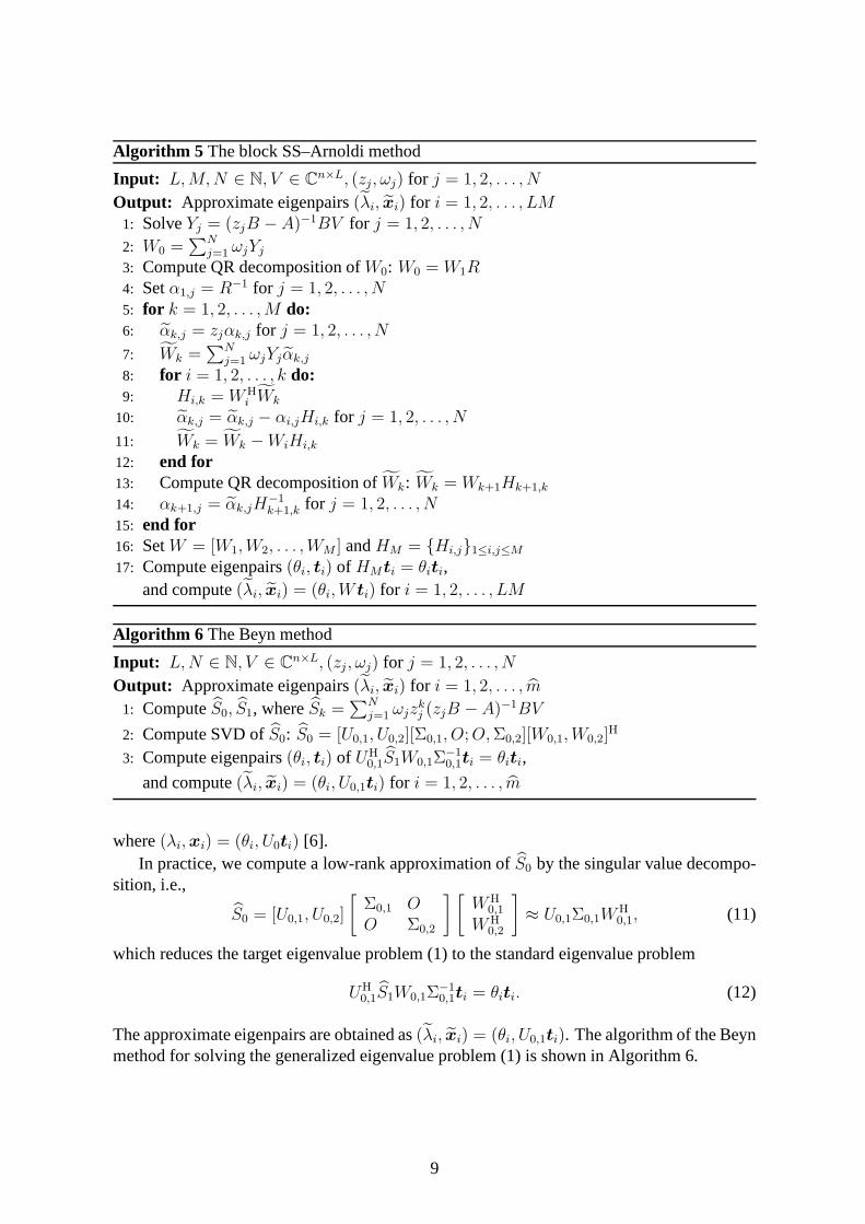
2.2.4 The block SS–Arnoldi method

From Theorems 2 and 3 and the definition ofCΩ := QΩJΩQHΩ, we have the following three

theorems [13].

Theorem 5. The subspaceR(S) can be expressed as the block Krylov subspace associatedwith the matrixCΩ:

R(S) = K

M(CΩ, S0).

7

Theorem 6. Let m be the number of target eigenvalues (counting multiplicity). Then, ifrank(S) = m, the target eigenvalue problem(1) is equivalent to a standard eigenvalueproblem of the form

CΩxi = λixi, xi ∈ R(S) = K

M(CΩ, S0). (8)

Theorem 7. AnyEk ∈ B

k (CΩ, S0) has the following formula:

Ek =1

2πi

∮

Γ

k−1∑

i=0

zi(zB − A)−1BV αidz, αi ∈ CL×L.

Then, the matrix multiplication ofCΩ byEk becomes

CΩEk =1

2πi

∮

Γ

z

k−1∑

i=0

zi(zB − A)−1BV αidz.

From Theorems 5 and 6, we observe that the target eigenpairs(λi,xi), λi ∈ Ω can becomputed by the block Arnoldi method with the block Krylov subspaceK

M(CΩ, S0) forsolving the standard eigenvalue problem (8). Here, we note that the matrixCΩ is not explicitlyconstructed. Instead, the matrix multiplication ofCΩ can be computed via the contour integralusing Theorem 7. By approximating the contour integral by a numerical integration rule, thealgorithm of the block SS–Arnoldi method is derived (Algorithm 5).

A low-rank approximation technique to reduce the computational costs and improve sta-bility is not applied in the current version of the block SS–Arnoldi method [13]. Improve-ments of the block SS–Arnoldi method has been developed in [14].

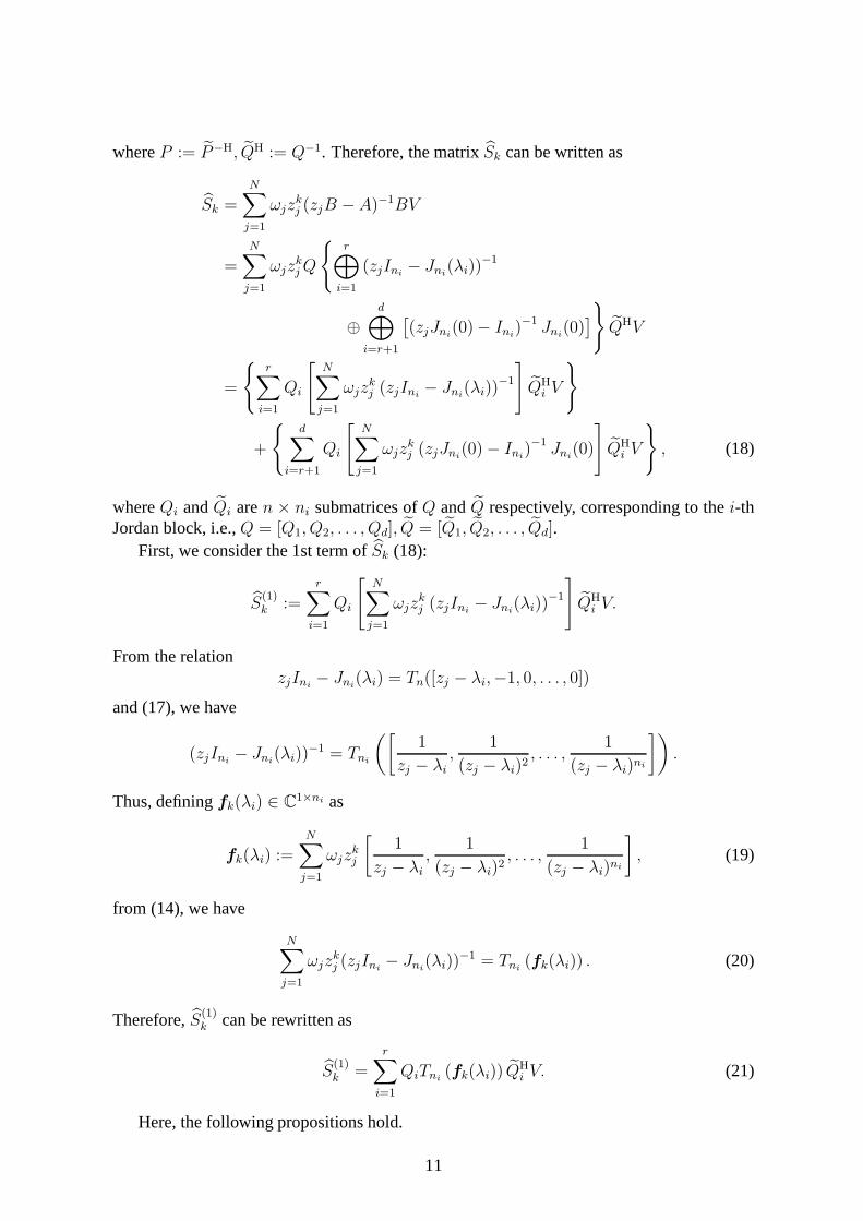
2.2.5 The Beyn method

The Beyn method is a nonlinear eigensolver based on the contour integral [6]. In this subsec-tion, we consider the algorithm of the Beyn method for solving the generalized eigenvalueproblem (1).

Let the singular value decomposition ofS0 beS0 = U0Σ0WH0 , whereU0 ∈ Cn×m,Σ0 =

diag(σ1, σ2, . . . , σm),W0 ∈ CL×m andrank(S0) = m. Then, from Theorem 2, we have

S0 = QΩQHΩV = U0Σ0W

H0 , S1 = QΩJΩQ

HΩV. (9)

SinceR(QΩ) = R(U0), we obtain

QΩ = U0Z, Z = UH0 QΩ ∈ C

m×m, (10)

whereZ is nonsingular. With (9) and (10), we findU0ZQHΩV = U0Σ0W

H0 and thusQH

ΩV =Z−1Σ0W

H0 . This leads to

UH0 S1 = ZJΩQ

HΩV = ZJΩZ

−1Σ0WH0 .

Therefore, we haveZJΩZ

−1 = UH0 S1W0Σ

−10 .

This means that the target eigenpairs(λi,xi), λi ∈ Ω are computed by solving

UH0 S1W0Σ

−10 ti = θiti,

8

Algorithm 5 The block SS–Arnoldi method

Input: L,M,N ∈ N, V ∈ Cn×L, (zj, ωj) for j = 1, 2, . . . , N

Output: Approximate eigenpairs(λi, xi) for i = 1, 2, . . . , LM1: SolveYj = (zjB − A)−1BV for j = 1, 2, . . . , N

2: W0 =∑N

j=1 ωjYj

3: Compute QR decomposition ofW0: W0 = W1R4: Setα1,j = R−1 for j = 1, 2, . . . , N5: for k = 1, 2, . . . ,M do:6: αk,j = zjαk,j for j = 1, 2, . . . , N

7: Wk =∑N

j=1 ωjYjαk,j

8: for i = 1, 2, . . . , k do:9: Hi,k = WH

i Wk

10: αk,j = αk,j − αi,jHi,k for j = 1, 2, . . . , N

11: Wk = Wk −WiHi,k

12: end for13: Compute QR decomposition ofWk: Wk = Wk+1Hk+1,k

14: αk+1,j = αk,jH−1k+1,k for j = 1, 2, . . . , N

15: end for16: SetW = [W1,W2, . . . ,WM ] andHM = Hi,j1≤i,j≤M

17: Compute eigenpairs(θi, ti) of HMti = θiti,and compute(λi, xi) = (θi,W ti) for i = 1, 2, . . . , LM

Algorithm 6 The Beyn method

Input: L,N ∈ N, V ∈ Cn×L, (zj , ωj) for j = 1, 2, . . . , N

Output: Approximate eigenpairs(λi, xi) for i = 1, 2, . . . , m

1: ComputeS0, S1, whereSk =∑N

j=1 ωjzkj (zjB −A)−1BV

2: Compute SVD ofS0: S0 = [U0,1, U0,2][Σ0,1, O;O,Σ0,2][W0,1,W0,2]H

3: Compute eigenpairs(θi, ti) of UH0,1S1W0,1Σ

−10,1ti = θiti,

and compute(λi, xi) = (θi, U0,1ti) for i = 1, 2, . . . , m

where(λi,xi) = (θi, U0ti) [6].In practice, we compute a low-rank approximation ofS0 by the singular value decompo-

sition, i.e.,

S0 = [U0,1, U0,2]

[Σ0,1 OO Σ0,2

] [WH

0,1

WH0,2

]≈ U0,1Σ0,1W

H0,1, (11)

which reduces the target eigenvalue problem (1) to the standard eigenvalue problem

UH0,1S1W0,1Σ

−10,1ti = θiti. (12)

The approximate eigenpairs are obtained as(λi, xi) = (θi, U0,1ti). The algorithm of the Beynmethod for solving the generalized eigenvalue problem (1) is shown in Algorithm 6.

9

3 Theoretical preliminaries for map building

As shown in Section 2, contour integral-based eigensolversare based on the property ofthe matricesS andSk (Theorems 2 and 3). The practical algorithms are then derived by anumerical integral approximation. As theoretical preliminaries for map building in Section 4,this section explores the properties of the approximated matricesS andSk. Here, we assumethat(zj, ωj) satisfy the following condition:

N∑

j=1

ωjzkj

= 0, k = 0, 1, . . . , N − 26= 0, k = −1

. (13)

If the matrix pencilzB−A is diagonalizable and(zj , ωj) satisfies condition (13), we have

Sk = CkS0, C = XrΛrXHr ,

whereXr = [x1,x2, . . . ,xr] is a matrix whose columns are eigenvectors correspondingto finite eigenvalues,Xr = [x1, x2, . . . , xr] is a submatrix ofX = X−H: XH

r Xr = I,andΛr = diag(λ1, λ2, . . . , λr); see [15]. In the following analysis, we introduce a similarrelationship in the case that the matrix pencilzB −A is non-diagonalizable. First, we definean upper triangular Toeplitz matrix as follows.

Definition 1. For a = [a1, a2, . . . , an] ∈ C1×n, defineTn(a) as ann× n triangular Toeplitzmatrix, i.e.,

Tn(a) :=

a1 a2 · · · an0 a1 · · · an−1...

. . . . . ....

0 · · · 0 a1

∈ C

n×n.

Let a = [a1, a2, . . . , an], b = [b1, b2, . . . , bn], c = [c1, c2, . . . , cn] ∈ C1×n andα, β ∈ C.Then, we have

αTn(a) + βTn(b) = Tn(αa+ βb), (14)

Tn(a)Tn(b) = Tn(c), ci =

i∑

j=1

ajbi−j+1, i = 1, 2, . . . , n. (15)

Lettingd = [α, β, 0, . . . , 0] ∈ C1×n, we also have

(Tn(d))k = Tn(d

(k)), d(k) =

[(k

0

)αkβ0,

(k

1

)αk−1β1, . . . ,

(k

n

)αk−n+1βn−1

], (16)

(Tn(d))−1 = Tn(d

(−1)), d(−1) =

[1

α,−

β

α2, . . . ,

(−β)n−1

αn

]. (17)

Using these relations (14)–(17), we analyze properties ofS andSk. From Theorem 1, wehave

(zB − A)−1 = Q

[r⊕

i=1

(zIni− Jni

(λi))−1 ⊕

d⊕

i=r+1

(zJni(0)− Ini

)−1

]PH,

B = P

[r⊕

i=1

Ini⊕

d⊕

i=r+1

Jni(0)

]QH,

10

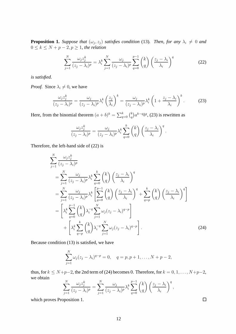
whereP := P−H, QH := Q−1. Therefore, the matrixSk can be written as

Sk =N∑

j=1

ωjzkj (zjB − A)−1BV

=N∑

j=1

ωjzkjQ

r⊕

i=1

(zjIni− Jni

(λi))−1

⊕d⊕

i=r+1

[(zjJni

(0)− Ini)−1 Jni

(0)]QHV

=

r∑

i=1

Qi

[N∑

j=1

ωjzkj (zjIni

− Jni(λi))

−1

]QH

i V

+

d∑

i=r+1

Qi

[N∑

j=1

ωjzkj (zjJni

(0)− Ini)−1 Jni

(0)

]QH

i V

, (18)

whereQi andQi aren × ni submatrices ofQ andQ respectively, corresponding to thei-thJordan block, i.e.,Q = [Q1, Q2, . . . , Qd], Q = [Q1, Q2, . . . , Qd].

First, we consider the 1st term ofSk (18):

S(1)k :=

r∑

i=1

Qi

[N∑

j=1

ωjzkj (zjIni

− Jni(λi))

−1

]QH

i V.

From the relationzjIni

− Jni(λi) = Tn([zj − λi,−1, 0, . . . , 0])

and (17), we have

(zjIni− Jni

(λi))−1 = Tni

([1

zj − λi

,1

(zj − λi)2, . . . ,

1

(zj − λi)ni

]).

Thus, definingfk(λi) ∈ C1×ni as

fk(λi) :=N∑

j=1

ωjzkj

[1

zj − λi

,1

(zj − λi)2, . . . ,

1

(zj − λi)ni

], (19)

from (14), we have

N∑

j=1

ωjzkj (zjIni

− Jni(λi))

−1 = Tni(fk(λi)) . (20)

Therefore,S(1)k can be rewritten as

S(1)k =

r∑

i=1

QiTni(fk(λi)) Q

Hi V. (21)

Here, the following propositions hold.

11

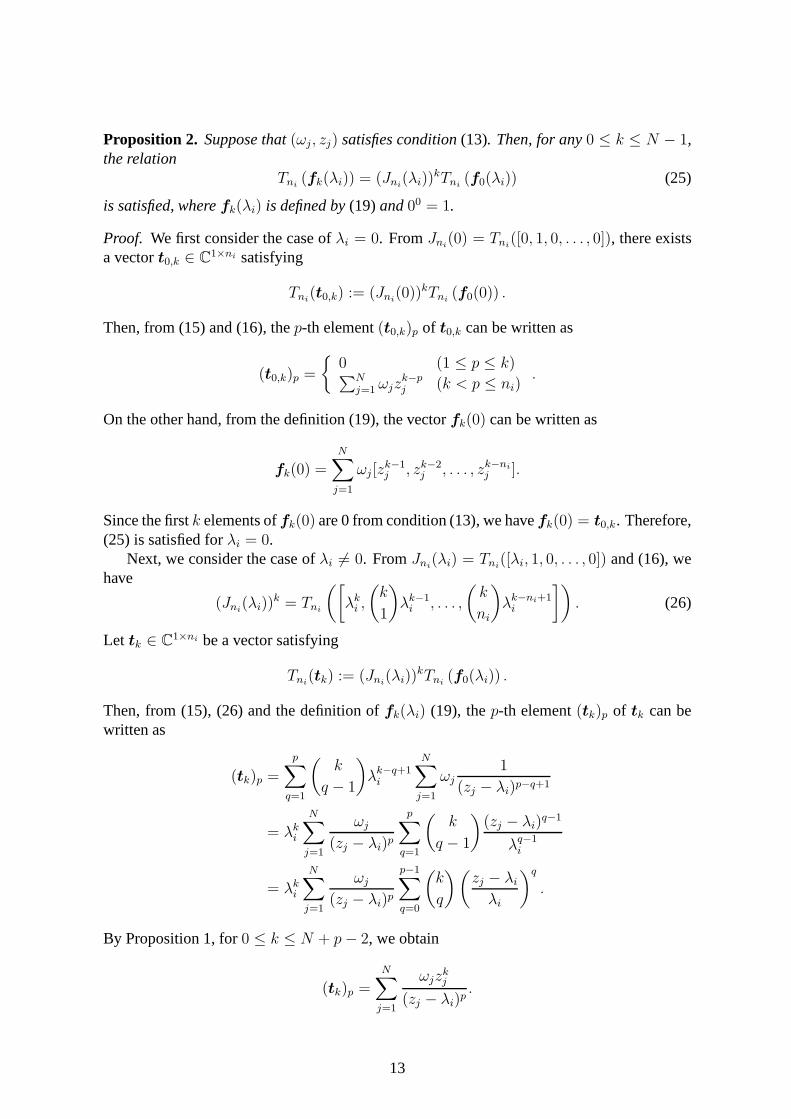
Proposition 1. Suppose that(ωj, zj) satisfies condition(13). Then, for anyλi 6= 0 and0 ≤ k ≤ N + p− 2, p ≥ 1, the relation

N∑

j=1

ωjzkj

(zj − λi)p= λk

i

N∑

j=1

ωj

(zj − λi)p

p−1∑

q=0

(k

q

)(zj − λi

λi

)q

(22)

is satisfied.

Proof. Sinceλi 6= 0, we have

ωjzkj

(zj − λi)p=

ωj

(zj − λi)pλki

(zjλi

)k

=ωj

(zj − λi)pλki

(1 +

zj − λi

λi

)k

. (23)

Here, from the binomial theorem(a + b)k =∑k

q=0

(k

q

)ak−qbq, (23) is rewritten as

ωjzkj

(zj − λi)p=

ωj

(zj − λi)pλki

k∑

q=0

(k

q

)(zj − λi

λi

)q

.

Therefore, the left-hand side of (22) is

N∑

j=1

ωjzkj

(zj − λi)p

=N∑

j=1

ωj

(zj − λi)pλki

k∑

q=0

(k

q

)(zj − λi

λi

)q

=

N∑

j=1

ωj

(zj − λi)pλki

[p−1∑

q=0

(k

q

)(zj − λi

λi

)q

+

k∑

q=p

(k

q

)(zj − λi

λi

)q]

=

[λki

p−1∑

q=0

(k

q

)λ−qi

N∑

j=1

ωj(zj − λi)q−p

]

+

[λki

k∑

q=p

(k

q

)λ−qi

N∑

j=1

ωj(zj − λi)q−p

]. (24)

Because condition (13) is satisfied, we have

N∑

j=1

ωj(zj − λi)q−p = 0, q = p, p+ 1, . . . , N + p− 2,

thus, fork ≤ N+p−2, the 2nd term of (24) becomes 0. Therefore, fork = 0, 1, . . . , N+p−2,we obtain

N∑

j=1

ωjzkj

(zj − λi)p=

N∑

j=1

ωj

(zj − λi)pλki

p−1∑

q=0

(k

q

)(zj − λi

λi

)q

,

which proves Proposition 1.

12

Proposition 2. Suppose that(ωj, zj) satisfies condition(13). Then, for any0 ≤ k ≤ N − 1,the relation

Tni(fk(λi)) = (Jni

(λi))kTni

(f0(λi)) (25)

is satisfied, wherefk(λi) is defined by(19)and00 = 1.

Proof. We first consider the case ofλi = 0. FromJni(0) = Tni

([0, 1, 0, . . . , 0]), there existsa vectort0,k ∈ C1×ni satisfying

Tni(t0,k) := (Jni

(0))kTni(f0(0)) .

Then, from (15) and (16), thep-th element(t0,k)p of t0,k can be written as

(t0,k)p =

0 (1 ≤ p ≤ k)∑N

j=1 ωjzk−pj (k < p ≤ ni)

.

On the other hand, from the definition (19), the vectorfk(0) can be written as

fk(0) =N∑

j=1

ωj [zk−1j , zk−2

j , . . . , zk−ni

j ].

Since the firstk elements offk(0) are 0 from condition (13), we havefk(0) = t0,k. Therefore,(25) is satisfied forλi = 0.

Next, we consider the case ofλi 6= 0. FromJni(λi) = Tni

([λi, 1, 0, . . . , 0]) and (16), wehave

(Jni(λi))

k = Tni

([λki ,

(k

1

)λk−1i , . . . ,

(k

ni

)λk−ni+1i

]). (26)

Let tk ∈ C1×ni be a vector satisfying

Tni(tk) := (Jni

(λi))kTni

(f0(λi)) .

Then, from (15), (26) and the definition offk(λi) (19), thep-th element(tk)p of tk can bewritten as

(tk)p =

p∑

q=1

(k

q − 1

)λk−q+1i

N∑

j=1

ωj

1

(zj − λi)p−q+1

= λki

N∑

j=1

ωj

(zj − λi)p

p∑

q=1

(k

q − 1

)(zj − λi)

q−1

λq−1i

= λki

N∑

j=1

ωj

(zj − λi)p

p−1∑

q=0

(k

q

)(zj − λi

λi

)q

.

By Proposition 1, for0 ≤ k ≤ N + p− 2, we obtain

(tk)p =

N∑

j=1

ωjzkj

(zj − λi)p.

13

Therefore, for0 ≤ k ≤ N − 1, we have

tk =

[N∑

j=1

ωjzkj

zj − λi

,

N∑

j=1

ωjzkj

(zj − λi)2, . . . ,

N∑

j=1

ωjzkj

(zj − λi)ni

]= fk(λi),

andTni

(fk(λi)) = Tni(tk) = (Jni

(λi))kTni

(f0(λi))

is satisfied, proving Proposition 2.

From Proposition 2, by substituting (25) into (21) and using(20), we obtain

S(1)k =

r∑

i=1

Qi (Jni(λi))

k Tni(f0(λi))Q

Hi V

=

r∑

i=1

Qi (Jni(λi))

k

[N∑

j=1

ωj (zjIni− Jni

(λi))−1

]QH

i V (27)

for any0 ≤ k ≤ N − 1.Now consider the 2nd term ofSk (18), i.e.,

S(2)k :=

d∑

i=r+1

Qi

[N∑

j=1

ωjzkj (zjJni

(0)− Ini)−1 Jni

(0)

]QH

i V.

From the relations

zjJni(0)− Ini

= Tni([−1, zj , 0, . . . , 0]),

Jni(0) = Tni

([0, 1, 0, . . . , 0])

and (15) and (17), we have

(zjJni(0)− I)−1 Jni

(0) = −Tni([0, 1, zj, z

2j , . . . , z

ni−2j ]).

In addition, from (14), we haveN∑

j=1

ωjzkj (zjJni

(0)− Ini)−1 Jni

(0)

= −Tni

([0,

N∑

j=1

ωjzkj ,

N∑

j=1

ωjzk+1j , . . . ,

N∑

j=1

ωjzk+ni−2j

]).

Here, because(zj , ωj) satisfies condition (13),

N∑

j=1

ωjzkj (zjJni

(0)− Ini)−1 Jni

(0) = O

is satisfied for any0 ≤ k ≤ N − ni. Therefore, letting

η := maxr+1≤i≤d

ni,

the 2nd term ofSk is O for any0 ≤ k ≤ N − η, i.e.,

S(2)k = O. (28)

From (27) and (28), we have the following theorems.

14

Theorem 8. Suppose that(ωj, zj) satisfies condition(13). Then, we have

Sk = CkS0, C = Q1:rJ1:rQH1:r,

for any0 ≤ k ≤ N − η, where

Q1:r := [Q1, Q2, . . . , Qr], Q1:r := [Q1, Q2, . . . , Qr], J1:r :=

r⊕

i=1

Jni(λi).

Proof. From (27) and (28), we have

Sk =

r∑

i=1

Qi(Jni(λi))

k

[N∑

j=1

ωj (zjIni− Jni

(λi))−1

]QH

i V,

for any0 ≤ k ≤ N − η. Here, we let

Fni:= Tni

(f0(λi)) =N∑

j=1

ωj (zjIni− Jni

(λi))−1 ,

F1:r :=

r⊕

i=1

Fni,

then we obtain

Sk =r∑

i=1

Qi (Jni(λi))

k FniQH

i V

= Q1:rJk1:rF1:rQ

H1:rV

= (Q1:rJ1:rQH1:r)

k(Q1:rF1:rQH1:rV )

= CkS0.

Therefore, Theorem 8 is proven.

Theorem 9. If (zj, ωj) satisfies condition(13), then the standard eigenvalue problem

Cxi = λixi, xi ∈ R(Q1:r), λi ∈ Ω ⊂ C, (29)

is equivalent to the generalized eigenvalue problem(1).

Proof. From the definition ofC := Q1:rJ1:rQH1:r, the matrixC has the same right eigenpairs

(λi,xi), i = 1, 2, . . . , r as the matrix pencilzB−A, i.e.,xi ∈ R(Q1:r). The other eigenvaluesof C are 0, and their corresponding eigenvectors are equivalent to the right eigenvectorsassociated with the infinite eigenvaluesλi = ∞ of zB − A, i.e.,xi 6∈ R(Q1:r). Therefore,Theorem 9 is proven.

15

4 Map of the relationships among contour integral-basedeigensolvers

Section 3 analyzed the properties of the approximated matricesS and Sk (Theorem 8) andintroduced the standard eigenvalue problem (29) equivalent to the target eigenvalue problem(1) (Theorem 9).

In this section, based on Theorems 8 and 9, we reconsider the algorithms of the contourintegral-based eigensolvers in terms of projection methods and map the relationships, focus-ing on their subspace used, the type of projection and the problem to which they are appliedimplicitly.

4.1 Reconsideration of the contour integral-based eigensolvers

As described in Section 2, the subspacesR(S) andR(Sk) contain only the target eigenvectorsxi, λi ∈ Ω based on Cauchy’s integral formula. In contrast, the subspacesR(S) andR(Sk)are rich in the component of the target eigenvectors as will be shown in Section 5.

4.1.1 The block SS–RR method and the FEAST eigensolvers

The block SS–RR method and the FEAST eigensolvers are easilyreconfigured as projectionmethods.

The block SS–RR method solvesAxi = λiBxi through the Rayleigh–Ritz procedure onR(S). The block SS–RR method (Algorithm 2) is derived using a low-rank approximationof the matrixS as shown in Section 2.2. SinceR(S) is rich in the component of the targeteigenvectors, the target eigenpairs are well approximatedby the Rayleigh–Ritz procedure.

The FEAST eigensolver conducts accelerated subspace iteration with the Rayleigh–Ritzprocedure. In each iteration of the FEAST eigensolver, the Rayleigh–Ritz procedure solvesAxi = λiBxi onR(S0). Like R(S) in the block SS–RR method,R(S0) is rich in the com-ponent of the target eigenvectors; therefore, the FEAST eigensolver also well approximatesthe target eigenpairs by the Rayleigh–Ritz procedure.

4.1.2 The block SS–Hankel method, the block SS–Arnoldi method and the Beyn method

From Theorem 8, we rewrite the block complex momentsµ

k of the block SS–Hankel methodas

µ

k = V HSk = V HCSk−1 = · · · = V HCkS0.

16

Thus, the block Hankel matricesH

M , H<M (7) become

H

M =

V HS0 V HS1 · · · V HSM−1

V HCS0 V HCS1 · · · V HCSM−1...

.... . .

...V HCM−1S0 V HCM−1S1 · · · V HCM−1SM−1

,

H<M =

V HCS0 V HCS1 · · · V HCSM−1

V HC2S0 V HC2S1 · · · V HC2SM−1...

.... . .

...V HCM S0 V HCM S1 · · · V HCM SM−1

,

respectively. Here, let

S := [V , CHV , (CH)2V , . . . , (CH)M−1V ].

Then, we haveH

M = SHS, H<M = SHCS.

Therefore, the generalized eigenvalue problem (6) is rewritten as

SHCSyi = θiSHSyi. (30)

In this form, the block SS–Hankel method can be regarded as a Petrov–Galerkin-type projec-tion method for solving the standard eigenvalue problem (29), i.e., the approximate solutionxi and the corresponding residualri := Cxi−θixi satisfyxi ∈ R(S) andri⊥R(S), respec-tively. Recognizing thatR(S) ⊂ R(Q1:r) and applying Theorem 9, we find that the blockSS–Hankel method obtains the target eigenpairs.

Since the Petrov–Galerkin-type projection method for (29)does not perform the (bi-)orthogonalization; that isSHS 6= I, (30) describes the generalized eigenvalue problem. Thepractical algorithm of the block SS–Hankel method (Algorithm 1) is derived from a low-rankapproximation of (30).

From Theorem 8, we haveR(S) = K

M(C, S0)

similar to Theorem 5. Therefore, the block SS–Arnoldi method can be regarded as a blockArnoldi method withK

M(C, S0) for solving the standard eigenvalue problem (29). Moreover,for M ≤ N − η, anyEM ∈ B

M(C, S0) can be written as

EM =

N∑

j=1

ωj

M−1∑

i=0

zij(zjB − A)−1BV αi, αi ∈ CL×L.

and the matrix multiplication ofC by EM is given by

CEM =

N∑

j=1

ωjzj

M−1∑

i=0

zij(zjB −A)−1BV αi.

similar to Theorem 7. Therefore, in each iteration, the matrix multiplication of C can beperformed by a numerical integration.

17

The Beyn method can be also regarded as a projection method for solving the standardeigenvalue problem (29). From the relationS1 = CS0 and the singular value decomposition(11) of S0, the coefficient matrix of the eigenvalue problem (12) obtained from the Beynmethod becomes

UH0,1S1W0,1Σ

−11 = UH

0,1CS0W0,1Σ−10,1 = UH

0,1CU0,1.

Therefore, the Byen method can be regarded as a Rayleigh–Ritz-type projection method onR(U0,1) for solving (29), whereR(U0,1) is obtained from a low-rank approximation ofS0.

4.2 Map of the contour integral-based eigensolvers

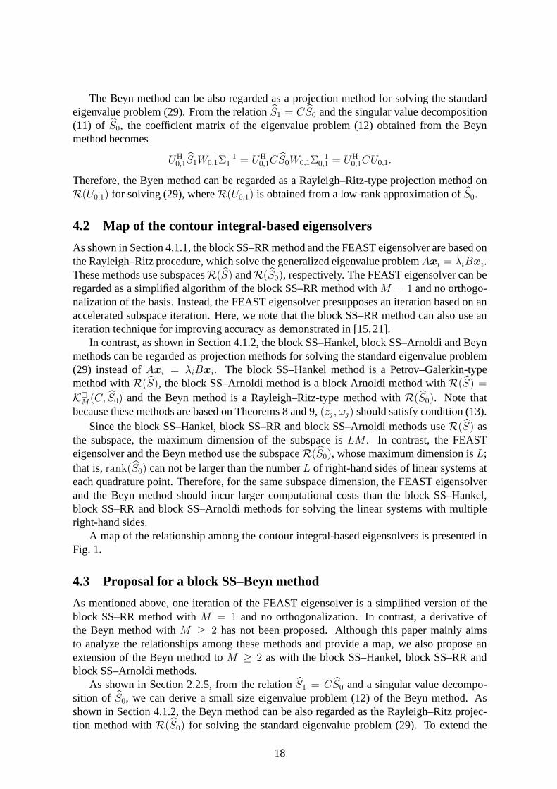
As shown in Section 4.1.1, the block SS–RR method and the FEAST eigensolver are based onthe Rayleigh–Ritz procedure, which solve the generalized eigenvalue problemAxi = λiBxi.These methods use subspacesR(S) andR(S0), respectively. The FEAST eigensolver can beregarded as a simplified algorithm of the block SS–RR method with M = 1 and no orthogo-nalization of the basis. Instead, the FEAST eigensolver presupposes an iteration based on anaccelerated subspace iteration. Here, we note that the block SS–RR method can also use aniteration technique for improving accuracy as demonstrated in [15,21].

In contrast, as shown in Section 4.1.2, the block SS–Hankel,block SS–Arnoldi and Beynmethods can be regarded as projection methods for solving the standard eigenvalue problem(29) instead ofAxi = λiBxi. The block SS–Hankel method is a Petrov–Galerkin-typemethod withR(S), the block SS–Arnoldi method is a block Arnoldi method withR(S) =

K

M(C, S0) and the Beyn method is a Rayleigh–Ritz-type method withR(S0). Note thatbecause these methods are based on Theorems 8 and 9,(zj , ωj) should satisfy condition (13).

Since the block SS–Hankel, block SS–RR and block SS–Arnoldimethods useR(S) asthe subspace, the maximum dimension of the subspace isLM . In contrast, the FEASTeigensolver and the Beyn method use the subspaceR(S0), whose maximum dimension isL;that is,rank(S0) can not be larger than the numberL of right-hand sides of linear systems ateach quadrature point. Therefore, for the same subspace dimension, the FEAST eigensolverand the Beyn method should incur larger computational coststhan the block SS–Hankel,block SS–RR and block SS–Arnoldi methods for solving the linear systems with multipleright-hand sides.

A map of the relationship among the contour integral-based eigensolvers is presented inFig. 1.

4.3 Proposal for a block SS–Beyn method

As mentioned above, one iteration of the FEAST eigensolver is a simplified version of theblock SS–RR method withM = 1 and no orthogonalization. In contrast, a derivative ofthe Beyn method withM ≥ 2 has not been proposed. Although this paper mainly aimsto analyze the relationships among these methods and provide a map, we also propose anextension of the Beyn method toM ≥ 2 as with the block SS–Hankel, block SS–RR andblock SS–Arnoldi methods.

As shown in Section 2.2.5, from the relationS1 = CS0 and a singular value decompo-sition of S0, we can derive a small size eigenvalue problem (12) of the Beyn method. Asshown in Section 4.1.2, the Beyn method can be also regarded as the Rayleigh–Ritz projec-tion method withR(S0) for solving the standard eigenvalue problem (29). To extendthe

18

The target GEP

block SS-RR

FEAST

blockSS-Hankel

Beyn

blockSS-Arnoldi

SEP with the same eigenpairs

Rayleigh-Ritz

(Implicit)

transformation

blockSS-Beyn

Subspaceiteration Petrov-Galerkin block Arnoldi

Rayleigh-Ritz

with high ordermoments

Fig. 1: A map of the relationship among the contour integral-based eigensolvers.

Beyn method, here we consider the Rayleigh–Ritz projectionmethod withR(S) for solving(29), i.e.,

UHCUti = θiti

whereS = UΣWH is a singular value decomposition ofS. Using Theorem 8, the coefficientmatrixUTCU is replaced as

UHCU = UHCSW1Σ−11 = UHS+W1Σ

−11 ,

whereS+ := [S1, S2, . . . , SM ] = CS.

In practice, we can also use a low-rank approximation ofS,

S = [U1, U2]

[Σ1 OO Σ2

] [WH

1

WH2

]≈ U1Σ1W

H1 .

Then, the reduced eigenvalue problem becomes

UH1 S+W1Σ

−11 ti = θiti.

The approximate eigenpairs are obtained as(λi, xi) = (θi, U1ti). In this paper, we call thismethod as the block SS–Beyn method and show it in Algorithm 7.

Both the block SS–RR method and the block SS–Beyn method are Rayleigh–Ritz-typeprojection methods withR(S). However, since the methods are targeted at different eigen-value problems, they have different definitions of the residual vector. Therefore, these meth-ods mathematically differ whenB 6= I. In contrast, the block SS–Arnoldi method and theblock SS–Beyn method without a low-rank approximation, i.e., m = LM , are mathemati-cally equivalent.

19

Algorithm 7 A block SS–Beyn method

Input: L,M,N ∈ N, V ∈ Cn×L, (zj, ωj) for j = 1, 2, . . . , N

Output: Approximate eigenpairs(λi, xi) for i = 1, 2, . . . , m

1: ComputeSk =∑N

j=1 ωjzkj (zjB − A)−1BV ,

and setS = [S0, S1, . . . , SM−1], S+ = [S1, S2, . . . , SM ]

2: Compute SVD ofS: S = [U1, U2][Σ1, O;O,Σ2][W1,W2]H

3: Compute eigenpairs(θi, ti) of UH1 S+W1Σ

−11 ti = θiti,

and compute(λi, xi) = (θi, U1ti) for i = 1, 2, . . . , m

5 Error analyses of the contour integral-based eigensolverswith an iteration technique

As shown in Section 2.2.3, the FEAST eigensolver is based on the iteration. Other iterativecontour integral-based eigensolvers have been designed toimprove the accuracy [15, 21].The basic concept is the iterative computation of the matrixS

(ℓ−1)0 , from the initial matrix

S(0)0 = V as follows:

S(ν)0 :=

N∑

j=1

ωj(zjB − A)−1BS(ν−1)0 , ν = 1, 2, . . . , ℓ− 1. (31)

The matricesS(ℓ)k andS(ℓ) are then constructed fromS(ℓ−1)

0 as

S(ℓ) := [S(ℓ)0 , S

(ℓ)1 , . . . , S

(ℓ)M−1], S

(ℓ)k :=

N∑

j=1

ωjzkj (zjB − A)−1BS

(ℓ−1)0 , (32)

andR(S(ℓ)0 ) andR(S(ℓ)) are used as subspaces rather thanR(S0) andR(S). Theℓ iterations

of the FEAST eigensolver can be regarded as a Rayleigh–Ritz-type projection method onR(S

(ℓ)0 ).

From the discussion in Section 3, the matrixS(ℓ)0 can be expressed as

S(ℓ)0 =

(Q1:rF1:rQ

H1:r

)ℓV.

Here, the eigenvalues of the linear operatorP := Q1:rF1:rQH1:r are given by

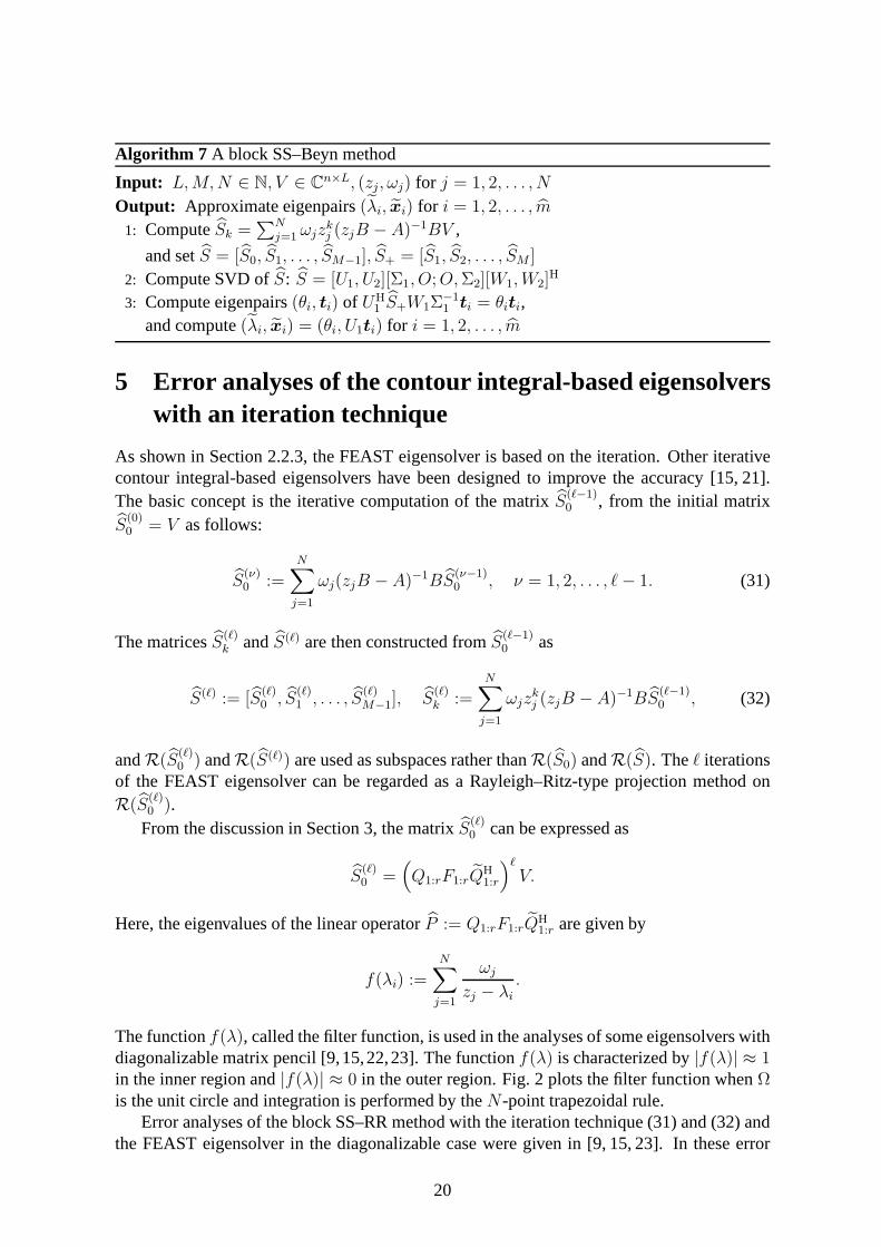
f(λi) :=

N∑

j=1

ωj

zj − λi

.

The functionf(λ), called the filter function, is used in the analyses of some eigensolvers withdiagonalizable matrix pencil [9,15,22,23]. The functionf(λ) is characterized by|f(λ)| ≈ 1in the inner region and|f(λ)| ≈ 0 in the outer region. Fig. 2 plots the filter function whenΩis the unit circle and integration is performed by theN-point trapezoidal rule.

Error analyses of the block SS–RR method with the iteration technique (31) and (32) andthe FEAST eigensolver in the diagonalizable case were givenin [9, 15, 23]. In these error

20

(a) On the real axis forN = 16, 32, 64.

(b) On the complex plane forN = 32.

Fig. 2: Magnitude of filter function|f(λ)| of theN-point trapezoidal rule for the unit circleregionΩ.

analyses, the block SS–RR method and the FEAST eigensolver were treated as projectionmethods with the subspacesR(S) andR(S0), respectively. In Section 4, we explained thatthe other contour integral-based eigensolvers are also projection methods with the subspacesR(S) andR(S0), but were designed to solve the standard eigenvalue problem(29). In thissection, we establish the error bounds of the contour integral-based eigensolvers with theiteration technique (31) and (32), omitting the low-rank approximation, in non-diagonalizablecases.

5.1 Error bounds of the block SS–RR method and the FEAST eigen-solver in the diagonalizable case

Let (λi,xi) be exact finite eigenpairs of the generalized eigenvalue problemAxi = λiBxi.Assume thatf(λi) are ordered by decreasing magnitude|f(λi)| ≥ |f(λi+1)|. DefineP(ℓ)

andPLM as orthogonal projectors onto the subspacesR(S(ℓ)) and the spectral projectorwith an invariant subspacespanx1,x2, . . . ,xLM, respectively. Assume that the matrixPLM [V, CV, . . . , CM−1V ] is full rank. Then, for each eigenvectorxi, i = 1, 2, . . . , LM ,there exists a unique vectorsi ∈ K

M(C, V ) such thatPLMsi = xi.In the diagonalizable case, for the error analysis of the block SS–RR method and the

FEAST eigensolver, the following inequality was given in [15] and [9,23] forM = 1:

‖(I − P(ℓ))xi‖2 ≤ αβi

∣∣∣∣f(λLM+1)

f(λi)

∣∣∣∣ℓ

, i = 1, 2, . . . , LM, (33)

whereα = ‖Xr‖2‖Xr‖2 andβi = ‖xi−si‖2. Note that, in the diagonalizable case, the linearoperatorP can be expressed asP = Xrf(Λr)X

Hr , wheref(Λr) := diag(f(λ1), f(λ2), . . . f(λr)).

An additional error bound is given in [15]:

‖(AP(ℓ) − λiBP(ℓ))xi‖2 ≤ γi‖(I − P(ℓ))xi‖2 ≤ αβiγi

∣∣∣∣f(λLM+1)

f(λi)

∣∣∣∣ℓ

, (34)

for i = 1, 2, . . . , LM , whereAP(ℓ) := P(ℓ)AP(ℓ), BP(ℓ) := P(ℓ)BP(ℓ) andγi = ‖P(ℓ)(A −λiB)(I − P(ℓ))‖2.

Inequality (33) determines the accuracy of the subspaceR(S), whereas inequality (34)defines the error bound of the block SS–RR method and the FEASTeigensolver.

21

5.2 Error bounds of the contour integral-based eigensolvers in the non-diagonalizable case

The constantα in (33) derives from the following inequality for a diagonalizable matrixGdiag = XDX−1

‖Gℓdiag‖2 ≤ ‖X‖2‖D

ℓ‖2‖X−1‖2 ≤ ‖X‖2‖X

−1‖2(ρ(Gdiag))ℓ,

whereρ(Gdiag) is the spectral radius ofGdiag. This inequality is extended to a non-diagonalizablematrixDnon = XJX−1 as follows:

‖Gℓnon‖2 ≤ ‖X‖2‖J

ℓ‖2‖X−1‖2 ≤ 2‖X‖2‖X

−1‖2ℓη−1(ρ(Gnon))

ℓ,

whereρ(Gnon) is the spectral radius ofGnon andη is the maximum size of the Jordan blocks.Using this inequality, the error bound of the contour integral-based eigensolvers in the non-diagonalizable case is given as

‖(I −P(ℓ))xi‖2 ≤ α′βiℓη−1

∣∣∣∣f(λLM+1)

f(λi)

∣∣∣∣ℓ

, i = 1, 2, . . . , LM, (35)

whereα′ = 2‖Q1:r‖2‖Q1:r‖2. From (35), the error bound of the block SS–RR method andthe FEAST eigensolver in the non-diagonalizable case is given by

‖(AP(ℓ) − λiBP(ℓ))xi‖2 ≤ γi‖(I − P(ℓ))xi‖2 ≤ α′βiγiℓη−1

∣∣∣∣f(λLM+1)

f(λi)

∣∣∣∣ℓ

, (36)

for i = 1, 2, . . . LM .The inequality (36) derives from the error bound of the Rayleigh–Ritz procedure for gen-

eralized eigenvalue problemsAxi = λiBxi. From the error bound of the Rayleigh–Ritzprocedure for standard eigenvalue problems [18, Theorem 4.3], we derive the error bound ofthe block SS–Arnoldi and block SS–Beyn methods as

‖(CP(ℓ) − λiI)P(ℓ)xi‖2 ≤ γ′‖(I − P(ℓ))xi‖2 ≤ α′βiγ

′ℓη−1

∣∣∣∣f(λLM+1)

f(λi)

∣∣∣∣ℓ

, (37)

for i = 1, 2, . . . , LM , whereCP(ℓ) := P(ℓ)CP(ℓ) andγ′ = ‖P(ℓ)C(I −P(ℓ))‖2.In addition, letQ be the oblique projector ontoR(S(ℓ)) and orthogonal toR(S). Then,

from the error bound of the Petrov–Galerkin-type projection method for standard eigenvalueproblems [18, Theorem 4.7], the error bound of the block SS–Hankel method is derived asfollows:

‖(CQ

P(ℓ) − λiI)P(ℓ)xi‖2 ≤ γ′′

i ‖(I − P(ℓ))xi‖2 ≤ α′βiγ′′i ℓ

η−1

∣∣∣∣f(λLM+1)

f(λi)

∣∣∣∣ℓ

, (38)

for i = 1, 2, . . . , LM , whereCQ

P(ℓ) := QCP(ℓ) andγ′′i = ‖Q(C − λiI)(I −P(ℓ))‖2.

Error bounds (36), (37) and (38) indicate that given a sufficiently large subspace, i.e.,|f(λLM+1)/f(λi)|

ℓ ≈ 0, the contour integral-based eigensolvers can obtain the accurate tar-get eigenpairs even if some eigenvalues exist outside but near the region and the target matrixpencil is non-diagonalizable.

22

6 Numerical experiments

This paper mainly aims to analyze the relationships among the contour integral-based eigen-solvers and to map these relationships; although, in this section, the efficiency of the blockSS–Hankel, block SS–RR, block SS–Arnoldi and block SS–Beynmethods are compared innumerical experiments withM = 1, 2, 4, 8 and16.

These methods compute 1000 eigenvalues in the interval[−1, 1] and the correspondingeigenvectors of a real symmetric generalized eigenvalue problem with 20000 dimensionaldense and random matrices.Γ is an ellipse with center 0 and major and minor axises 1and 0.1, respectively. The parameters are(L,M) = (4096, 1), (2048, 2), (1024, 4), (512, 8),(256, 16) (note thatLM = 4096) andN = 32. Because of a symmetry of the problem, thenumber of required linear systems isN/2 = 16. For the low-rank approximation, we usedsingular valuesσi satisfyingσi/σ1 ≥ 10−14 and their corresponding singular vectors, whereσ1 is the largest singular value.

The numerical experiments were carried out in double precision arithmetic on 8 nodes ofCOMA at CCS, University of Tsukuba. COMA has two Intel Xeon E5-2670v2 (2.5 GHz)and two Intel Xeon Phi 7110P (61 cores) per node. In these numerical experiments, we usedonly the CPU part. The algorithms were implemented in Fortran 90 and MPI, and executedwith 8 [node]× 2 [process/node]× 8 [thread/process].

The numerical results are presented in Table 1. First, we consider the numerical rankm.ComparingM dependence of the numerical rankm in the block SS–Hankel, block SS–RRand block SS–Beyn methods, we observe that the numerical rank m increases with increasingM . This is causally related to the property of the subspaceK

M(C, V ), becauseS is writtenas

S =(Q1:rF1:rQ

H1:r

)[V, CV, . . . , CM−1V ].

ForM = 1, the subspaceK

1 (C, V ) = R(V ) is unbiased for all eigenvectors, sinceV is arandom matrix. On the other hand, forM ≥ 2, the subspaceK

M(C, V ) contains eigenvectorscorresponding exterior eigenvalues well. Therefore, for computing interior eigenvalues, thenumerical rankm for M = 16 is expected to be larger than forM = 1.

Next, we consider the computation time. The computation times of the LU factorization,forward and back substitutions and the other computation time including the singular valuedecomposition and orthogonalization are denoted bytLU, tSolve, tOther, respectively. The totalcomputation time is also denoted bytTotal. We observe, from Table 1, that the most time-consuming part is to solve linear systems with multiple-right hand sides (tLU + tSolve). Inparticular,tSolve is much larger forM = 1 than forM = 16, because the number of right-hand sides forM = 1 is 16 times larger than forM = 16. Consequently,tTotal increases withdecreasingM .

We now focus ontOther. The block SS–Arnoldi method consumes much greatertOther

than the other methods because its current version applies no low-rank approximation tech-nique to reduce the computational costs and improve the stability [13]. For the block SS–Hankel, block SS–RR and block SS–Beyn methods,tOther is smaller asM and the numeri-cal rankm are smaller. In addition, the block SS–Hankel method consumes smallesttOther

among tested methods, because it performs no matrix orthogonalization.Finally, we consider the accuracy of the computed eigenpairs. The block SS–Hankel and

block SS–Arnoldi methods are less accurate than the other methods, specifically forM = 16.This result is attributed to no matrix orthogonalization inthe block SS–Hankel method, and

23

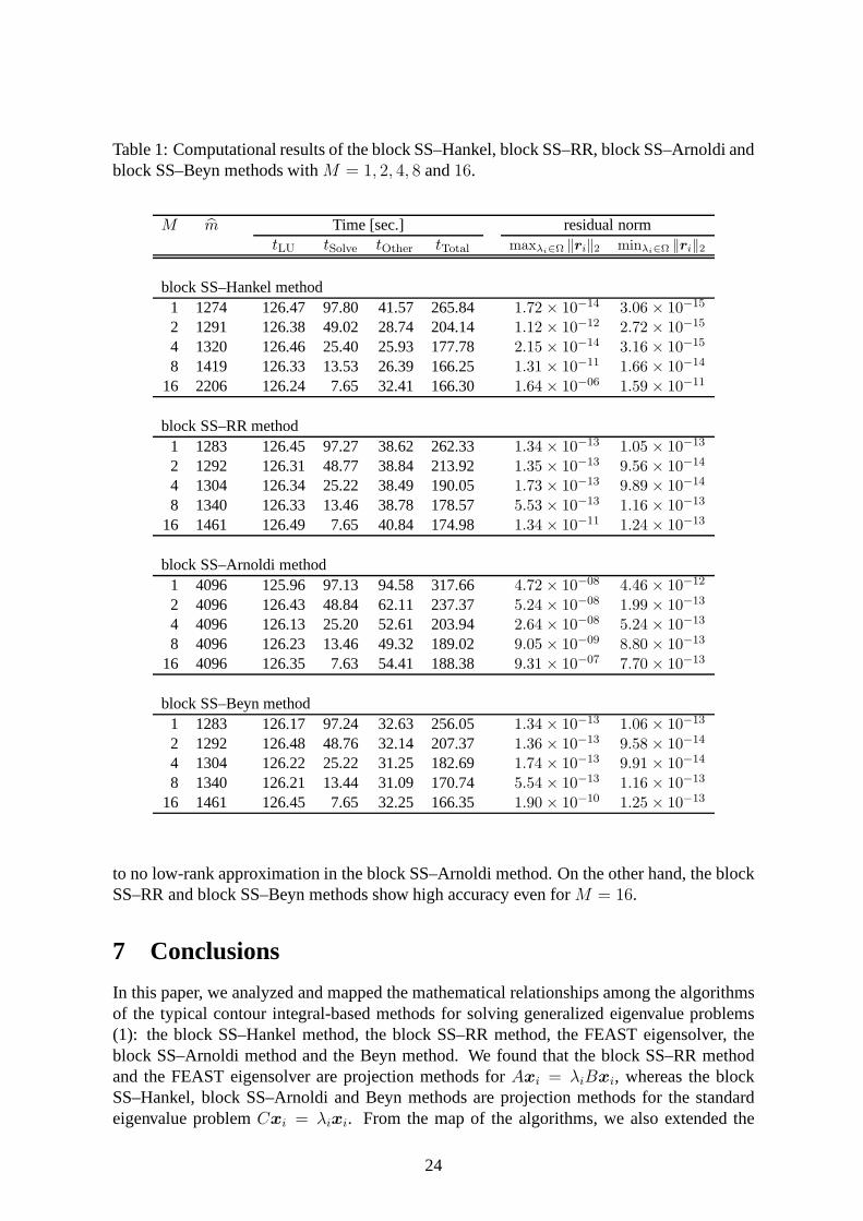
Table 1: Computational results of the block SS–Hankel, block SS–RR, block SS–Arnoldi andblock SS–Beyn methods withM = 1, 2, 4, 8 and16.

M m Time [sec.] residual normtLU tSolve tOther tTotal maxλi∈Ω ‖ri‖2 minλi∈Ω ‖ri‖2

block SS–Hankel method1 1274 126.47 97.80 41.57 265.84 1.72 × 10

−143.06 × 10

−15

2 1291 126.38 49.02 28.74 204.14 1.12 × 10−12

2.72 × 10−15

4 1320 126.46 25.40 25.93 177.78 2.15 × 10−14

3.16 × 10−15

8 1419 126.33 13.53 26.39 166.25 1.31 × 10−11

1.66 × 10−14

16 2206 126.24 7.65 32.41 166.30 1.64 × 10−06

1.59 × 10−11

block SS–RR method1 1283 126.45 97.27 38.62 262.33 1.34 × 10

−131.05 × 10

−13

2 1292 126.31 48.77 38.84 213.92 1.35 × 10−13

9.56 × 10−14

4 1304 126.34 25.22 38.49 190.05 1.73 × 10−13

9.89 × 10−14

8 1340 126.33 13.46 38.78 178.57 5.53 × 10−13

1.16 × 10−13

16 1461 126.49 7.65 40.84 174.98 1.34 × 10−11

1.24 × 10−13

block SS–Arnoldi method1 4096 125.96 97.13 94.58 317.66 4.72 × 10

−084.46 × 10

−12

2 4096 126.43 48.84 62.11 237.37 5.24 × 10−08

1.99 × 10−13

4 4096 126.13 25.20 52.61 203.94 2.64 × 10−08

5.24 × 10−13

8 4096 126.23 13.46 49.32 189.02 9.05 × 10−09

8.80 × 10−13

16 4096 126.35 7.63 54.41 188.38 9.31 × 10−07

7.70 × 10−13

block SS–Beyn method1 1283 126.17 97.24 32.63 256.05 1.34 × 10

−131.06 × 10

−13

2 1292 126.48 48.76 32.14 207.37 1.36 × 10−13

9.58 × 10−14

4 1304 126.22 25.22 31.25 182.69 1.74 × 10−13

9.91 × 10−14

8 1340 126.21 13.44 31.09 170.74 5.54 × 10−13

1.16 × 10−13

16 1461 126.45 7.65 32.25 166.35 1.90 × 10−10

1.25 × 10−13

to no low-rank approximation in the block SS–Arnoldi method. On the other hand, the blockSS–RR and block SS–Beyn methods show high accuracy even forM = 16.

7 Conclusions

In this paper, we analyzed and mapped the mathematical relationships among the algorithmsof the typical contour integral-based methods for solving generalized eigenvalue problems(1): the block SS–Hankel method, the block SS–RR method, theFEAST eigensolver, theblock SS–Arnoldi method and the Beyn method. We found that the block SS–RR methodand the FEAST eigensolver are projection methods forAxi = λiBxi, whereas the blockSS–Hankel, block SS–Arnoldi and Beyn methods are projection methods for the standardeigenvalue problemCxi = λixi. From the map of the algorithms, we also extended the

24

existing Beyn method toM ≥ 2. Our numerical experiments indicated that increasingMreduces the computational costs (relative toM = 1).

In future, we will compare the efficiencies of these methods in solving large, real-lifeproblems. We also plan to analyze the relationships among contour integral-based nonlineareigensolvers.

Acknowledgements

The authors would like to thank Dr. Kensuke Aishima, The University of Tokyo for his valu-able comments. The authors are also grateful to an anonymousreferee for useful comments.

References

[1] J. Asakura, T. Sakurai, H. Tadano, T. Ikegami, K. Kimura,A numerical method fornonlinear eigenvalue problems using contour integrals, JSIAM Letters,1(2009), 52–55.

[2] J. Asakura, T. Sakurai, H. Tadano, T. Ikegami, K. Kimura,A numerical method forpolynomial eigenvalue problems using contour integral, Japan J. Indust. Appl. Math,27(2010), 73–90.

[3] A. P. Austin, P. Kravanja, L. N. Trefethen, Numerical algorithms based on analyticfunction values at roots of unity, SIAM J. Numer. Anal.,52(2014), 1795–1821.

[4] A. P. Austin, L. N. Trefethen, Computing eigenvalues of real symmetric matrices withrational filters in real arithmetic, SIAM J. Sci. Comput.,37(2015), A1365–A1387.

[5] M. van Barel, P. Kravanja, Nonlinear eigenvalue problems and contour integrals, J.Comput. Appl. Math.,292(2016), 526–540.

[6] W.-J. Beyn, An integral method for solving nonlinear eigenvalue problems, Lin. Alg.Appl., 436(2012), 3839–3863.

[7] H. Fang, Y. Saad, A filtered Lanczos procedure for extremeand interior eigenvalueproblems, SIAM J. Sci. Comput.,34(2012), A2220–A2246.

[8] M. H. Gutknecht, Block Krylov space methods for linear systems with multiple right-hand sides: an introduction, in: proc. of Modern Mathematical Models, Methods andAlgorithms for Real World Systems (A.H. Siddiqi, I.S. Duff,and O. Christensen, eds.),420–447, Anamaya Publishers, New Delhi, India, 2007.

[9] S. Guttel, E. Polizzi, T. Tang, G. Viaud, Zolotarev quadrature rules and load balancingfor the FEAST eigensolver, arXiv:1407.8078.

[10] T. Ikegami, T. Sakurai, U. Nagashima, A filter diagonalization for generalized eigen-value problems based on the Sakurai-Sugiura projection method, Technical Report ofDepartment of Computer Science, University of Tsukuba (CS-TR), (2008), CS-TR-08-13.

25

[11] T. Ikegami, T. Sakurai, U. Nagashima, A filter diagonalization for generalized eigen-value problems based on the Sakurai-Sugiura projection method, J. Comput. Appl.Math.,233(2010), 1927–1936.

[12] T. Ikegami, T. Sakurai, Contour integral eigensolver for non-Hermitian systems: aRayleigh-Ritz-type approach, Taiwan. J. Math.,14(2010), 825–837.

[13] A. Imakura, L. Du, T. Sakurai, A block Arnoldi-type contour integral spectral projec-tion method for solving generalized eigenvalue problems, Applied Mathematics Letters,32(2014), 22–27.

[14] A. Imakura, L. Du, T. Sakurai, Communication-AvoidingArnoldi-type contour integral-based eigensolver (in Japanese), in: proc. of Annual meeting of JSIAM, 2014.

[15] A. Imakura, L. Du, T. Sakurai, Error bounds of Rayleigh–Ritz type contour integral-based eigensolver for solving generalized eigenvalue problems, Numer. Alg.,71(2016),103–120.

[16] P. Kravanja, T. Sakurai, M. van Barel, On locating clusters of zeros of analytic functions,BIT, 39(1999), 646–682.

[17] E. Polizzi, A density matrix-based algorithm for solving eigenvalue problems, Phys.Rev. B,79(2009), 115112.

[18] Y. Saad, Numerical Methods for Large Eigenvalue Problems, 2nd edition, SIAM,Philadelphia, PA, (2011).

[19] T. Sakurai, H. Sugiura, A projection method for generalized eigenvalue problems usingnumerical integration, J. Comput. Appl. Math.,159(2003), 119–128.

[20] T. Sakurai, H. Tadano, CIRR: a Rayleigh-Ritz type method with counter integral forgeneralized eigenvalue problems, Hokkaido Math. J.,36(2007), 745–757.

[21] T. Sakurai, Y. Futamura, H. Tadano, Efficient parameterestimation and implementationof a contour integral-based eigensolver, J. Algorithms Comput. Technol.,7(2014), 249–269.

[22] G. Schofield, J. R. Chelikowsky, Y. Saad, A spectrum slicing method for the Kohn-Shamproblem, Comput. Phys. Commun.,183(2012), 497–505.

[23] P. T. P. Tang, E. Polizzi, FEAST as a subspace iteration eigensolver accelerated byapproximate spectral projection, SIAM J. Matrix Anal. Appl., 35(2014), 354–390.

[24] G. Yin, R. H. Chan, M.-C. Yeung, A FEAST algorithm for generalized non-Hermitianeigenvalue problems, arXiv:1404.1768.

[25] S. Yokota, T. Sakurai, A projection method for nonlinear eigenvalue problems usingcontour integrals, JSIAM Letters,5(2013), 41–44.

[26] Y. Zhou, Y. Saad, M. L. Tiago, J. R. Chelikowsky, Self-consistent-field calculationsusing Chebyshev-filtered subspace iteration, J. Comput. Physics,219(2006), 172–184.

26