ISSN: 2766-9823 Volume 3, 2021 Solving inverse heat ...

Solving inverse heat conduction problems by usingTikhonov regularization in combination with the

genetic algorithmMohammad Reza Shahnazari

Dept. Mech. EngineeringK. N. Toosi Uni. of Technology

Tehran, [email protected]

Alireza RoohiShaliDept. Mech. Engineering

K. N. Toosi Uni. of TechnologyTehran, Iran

[email protected]

Ali SaberiDept. Mech. Engineering

K. N. Toosi Uni. of TechnologyTehran, Iran

[email protected]

Abstract—It is well-known that inverse heat conduction prob-lems (IHCPs) are severely lll-posed, which means that smallperturbations in data may cause extremely large errors inthe solution. This paper introduces an accurate method forsolving inverse problems, as solution procedure, we use Tikhonovregularization in combination with the genetic algorithm. Find-ing the regularization parameter as the decisive parameter ismodeled by this method, a few sample problems were solvedto investigate the efficiency and accuracy of the method. Alinear sum of fundamental solutions with unknown constantcoefficients assumed as an approximated solution to the sampleIHCP problem and collocation method is used to minimizeresidues in the collocation points. In this contribution, we useMorozov’s discrepancy principle and Quasi-Optimality criterionfor defining the objective function, which must be minimized toyield the value of the optimum regularization parameter.

Index Terms—Inverse Heat Transfer, Tikhonov regularization,Genetic algorithms, III-Posed Problems, Morozov’s discrepancyprinciple.

I. INTRODUCTION

Inverse problems have wide applications in technologicaland scientific fields [1].The primary purpose of solving theseproblems is to obtain solution indirectly. The main reasonfor the emergence of the inverse heat transfer problems isnot knowing boundary conditions or difficulty in accessingboundaries. Therefore, to solve the problem without havingboundary conditions, it is necessary to have additional infor-mation, which is usually obtained by the sensors installed in anaccessible place. Therefore, with empirical data, it is possibleto estimate the conditions needed to solve the problem withoutdirect measurements or access to boundary locations.

In direct heat transfer problems, geometry, boundary con-ditions, initial conditions, and thermo-physical properties areknown, and the purpose is to calculate the temperature dis-tribution inside the solution domain. In the case of inverseheat transfer, one or some information are unknown, and thepurpose is to estimate them by using additional informationsuch as the measured temperatures inside the solution domain.

The main difficulty in solving inverse problems is that theyare almost always severely ill-posed. A problem is called well-posed, according to Hadamard [2] if there exists a unique

solution to it that continuously changes with input data. Theinverse solution is extremely sensitive to measurement errors,and even the smallest in inputs may cause a significant error inthe final approximation of the boundary conditions, therefore,regularization is required for solving inverse problems.

Since IHCPs are incredibly diverse, their solution alsorequires different strategies. On the one hand, solving methodscan be classified into three different classes: analytical, numer-ical, and experimental solutions. Of course, in some cases, acombination of the mentioned methods can be used for solvingthe problem. Analytical methods are often useful in solvinglinear problems, but numerical methods such as the FiniteDifference method, finite element method, and boundary ele-ments are applied in solving nonlinear and multidimensionalproblems. In 1960, Stolz showed that frequent use of tiny timesteps results in instability in the solution of such problems[3]. It can be seen that using small time steps has the oppositeeffect on inverse heat conduction problems (IHCPs) comparedto numerical solutions of the direct heat conduction equation.

Another method that uses the regularization technique isthe conjugate gradient method with an adjoint problem, whichis developed and suggested in detail by Alifanov [4], Zisnikand Orlande [5]. The conjugate gradient method minimizesan objective function, at each iteration, choosing a new guessby taking the old assumption and tacking on an additionalterm that pushes the solution closer to the optimal one. Thisregularization technique can also be used to solve linear andnonlinear inverse problems or parametric estimations.

Tikhonov and Arsenin introduced Tikhonov and IterativeRegularization Methods [6]. This method is usually providedas a whole domain solution in which all the components ofheat flux are estimated for all times and spatial locations si-multaneously. Different approaches have been proposed in theliterature for the solution of IHCPs, and generally, a specificsolution for a particular problem cannot be applied for otherproblems. Various analytical and numerical methods have beenproposed for solving IHCPs. The special sequential functiondeveloped by Beck [7], is a sequential method steppingforward in time, based on least squares method and Duhamel

ISSN: 2766-9823 Volume 3, 2021

60

theorem. The complex mathematics in estimating componentsof the heat flux in different times and spatial locations is afundamental problem in the mentioned algorithm. In 1991,Hensel did some research on the analytical transfer functionto solve inverse heat conduction problems. He presented aninverse heat method for a one-dimensional case using anadjoint algorithm with a frequency domain [8].

In 1996, Lesnic et al. proposed another way to solve theIHCPs. In this method, the least squares regularization and en-ergy method have been introduced into the boundary elementmethod (BEM) formulation. The numerical results obtainedusing this technique has the advantage of not needing to meshgeneration in all domain, unlike the finite element methodor finite difference method [9], [10]. Yeun et al. dealt withthe smooth fitting problem using the genetic programmingalgorithm, they presented a novel approach for choosing theregularization parameter and compared the result with generalcross-validation (GCV) B-Splines [11].

Several researchers have proposed combinations of themethod used in reference [7], which seeks to minimize theproblems involved in measuring errors. As suggested byKeanini et al. In 2005, the goal is to achieve better stability. Inthis case, they have proposed a modified sequential functionfor solving stability of parabolic thermal conduction problem.This method uses computational steps that are larger than thesampled intervals, and future time intervals are all set equal tothe time interval in the data [12]. In 2008, Slota et al. combinedthe Tihonov regulation method and the particle swarm opti-mization algorithm, which is a stochastic optimization method,for approximating the heat source without the prior informa-tion of the functional form in temperature-dependent unsteadyheat conduction problem and compared the results with theconjugate gradient method [13]. Ajith and et al. Applied alattice Boltzmann method (LMB), finite volume method andgenetic algorithm approach to study the effect of modelingtools for the design of high-temperature heater enclosures in a2-D geometry [14]. Stephany et al. presented a regularizationtechnique applied to an inverse radiation-convection problemformulated as a finite dimensional optimization problem andsolved by hybridization of the ant colony optimization (ACO)with the Levenberg–Marquardt method [15].

Singh and Das presented the thermal investigation of aporous stepped fin made from different ceramic porous materi-als Al and SiC; they used the approximate analytical Adomiandecomposing method to solve the nonlinear problem alongwith the Newton–Raphson method [16]. Some researchersapplied an inverse algorithm based on the conjugate gradientmethod and the discrepancy principle to estimate the unknowntime-dependent frictional heat flux at the interface of twocontacting surfaces [17], [18]. Dong et al. presented thealleviation of non-optimal regularization parameter influenceon the temperature distribution reconstruction accuracy inparticipating medium using coupled methods, i.e., two kindsof regularization methods (least square QR decomposition(LSQR) method and truncated singular value decomposition(TSVD) method) combined with genetic algorithm (GA) [19].

For some samples, even combinational methods with non-optimal regularization parameters can be more accuratelysolved than results obtained by LSQR or TSVD [20], [21]. In2015, Udayraj et al. examined three developed metaheuristicalgorithms, including ant colony optimization, cuckoo search,and particle swarm optimization for a class of heat trans-fer problems. Unknown boundary heat fluxes are estimatedfor conduction, convection, and coupled conduction–radiationproblems [22]. Heng et al. in 2016 used five types of Krillherd algorithms to optimize the geometric locations of thecontrol points and solved the inverse geometry design of atwo-dimensional radiative enclosure filling with participatingmedia [23].

In this research, the method of Tikhonov regularizationis combined with the genetic algorithm to solve the inverseproblem. A genetic algorithm is used to find the regulariza-tion parameter, which is the main problem of regularizationmethods.

II. THEORY

The definition of a well-posed problem was given byJacques and Hadamard for the first time, to understand whatkind of boundary conditions should be used for different typesof differential equations [24]. He believed that mathematicalmodels of physical phenomena should have the followingproperties: a solution exists, the solution is unique; the solutionchanges continuously with initial conditions. If one of theseproperties is violated, the problem is called ill-posed. Stablenumerical differentiation of noisy data, stable inversing of ill-posed matrices, parameter determination in a partial differen-tial equation, first order homogeneous differential equationsare examples of Ill-posed problems. Consider the followingill-posed problem in which K is a linear bounded operatorfrom X into Y :

Kθ = W, K : X → Y, (1)

Suppose that the right side is given with its approximationWδ in such a way that ‖W −Wδ‖ ≤ δ. Naturally, we needto find the approximate answer in the set Qδ : θ ∈ X :‖Kθ −Wθ‖ ≤ δ. In any case, in an ill-posed problem, wecannot take an arbitrary element xδ ∈ Qδ as an approximatesolution for problem (1), because θδ does not change contin-uously as Wδ changes. Satisfying equation ‖Kθ −Wθ‖ ≤ δdoes not guarantee that θδ is close to the desired response.Suppose that K is a bounded linear operator between Hilbertspaces X to Y [25] and then Jα has a unique minimum inθδ ∈ X , the minimum is the unique solution of the normalequation λθλ + K∗Kθλ = K∗W In which, for all x ∈ X ,Jλ(θ) = ‖Kθλ − W‖22 + λ‖θλ‖22 is defined as Tikhonov’sfunction. Rλ : Y → X , Rλ = (λI +K∗K)−1K∗.It can beproved that the operators form a regularization strategy withlimλ→0‖RλKθe − θe‖ ≤ lim

λ→0

‖z‖√λ

2 , θe = K∗z ∈ K ∗ (Y ), z ∈Y . This method is called Tikhonov regularization.

After approximation, the result will be:∥∥θλ,δ − θe∥∥ ≤ δ

2√λ

+‖z‖√λ

2:= E(λ) (2)

ISSN: 2766-9823 Volume 3, 2021

61

Theoretically, although ‖z‖ is not known, we can minimizethe E(λ) function to find the optimal value for the ‖z‖regularization parameter, e.g., in the posteriori method forchoosing parameter λ which is called Morozov’s discrepancyprinciple the value of is not required. Choosing an appropriateregularization parameter is a critical part of achieving anoptimal response. The most commonly used methods forselecting the regularization parameter are as follows.

A. Morozov’s discrepancy principle

In this method, it is proposed that λ(δ) > 0 be calculatedin such a way that the Tikhonov solution which correspondsto the following equation

λθλ,δ +K∗Kθλ,δ = K∗Wδ (3)

which is the minimizer of the following functional:

Jλ,δ(θλ,δ) := ‖Kθλ,δ −Wδ‖2 + λ‖θλ,δ‖2 (4)

satisfies‖Kθλ,δ −Wδ‖ = Wδ (5)

Therefore, λ choosing in this condition is sufficient to ensurethat, on the one hand, the difference is equal to δ and, on theother hand, λ is not too small [26].

B. Quasi-Optimality criterion

The Quasi-Optimality criterion [26] determines the valueλ > 0 in such a way that

Λ(λ) := λ2fTδ K(K∗K + λI)−4K∗fδ = min (6)

To obtain the regularization parameter, in this paper, we useMorozov’s discrepancy principle, which requires the distur-bance amplitude, and Quasi-Optimality criterion, which doesnot require disturbance amplitude. We can use derivatives,or different numerical root finding can be used to optimizethe objective functions of these two criterions, but doing thisfor any criterion requires separate calculations and derivationand root finding that complicates the work and raises com-putational costs, at the same time, there is no guarantee thatthe algorithm implemented converges. This paper presents anew high-precision meta-heuristic algorithm, which is easy tomodify and doesn’t produce complications when the objectivefunction changes, which then is applied to a sample problem. Itis clear that the solution in Tikhonov regularization depends onthe regularization parameter, which directly affects the degreeof approximation and the stability of the solution. In terms ofapproximation, the smaller the λ is the better and ‖θλ − θe‖will have a smaller value in a stable solution; but from thestability point of view, the bigger the λ is the better. Thekey in solving Tikhonov regularization method is finding theoptimal value for the regularization parameter. In Morozov’sdiscrepancy principle, the regularization parameter is chosenin such a way that:

‖Kθλ −Wδ‖22 = δ2 (7)

On the other hand, in the Quasi-Optimality criterion, the opti-mal regularization parameter is the minimizer of the followingobjective function.

Λ(λ) =1

λ2WTδ K(KTK + λI)

−4KTWδ

(8)

Unlike Morozov’s discrepancy principle, in the Quasi-Optimality criterion, the magnitude of perturbations is notrequired. In this paper, a genetic algorithm is used to find theoptimal regularization parameter. The purpose is to optimizeone of the two following objective functions for obtaining theoptimal value of the regularization parameter.

Γ(λ) =∣∣∣‖Kθλ −Wδ‖22 − δ

2∣∣∣ (9)

Λ(λ) =1

λ2WTδ K(KTK + λI)

−4KTWδ

(10)

Initially, a population of monogenic chromosomes which theirgene value is λ is created, then by having the value of λfor each chromosome, αλ is calculated for each chromosome.Using θλ, the value of the objective functions Γ(λ) and Λ(λ)are calculated for each chromosome. Crossover and mutationoperations are performed to create offspring and mutatedchromosomes and the value of the objective functions arecalculated for them. The chromosomes are ranked accordingto the value of their objective function then, the best chro-mosomes make up the second generation according to theirrank, all of these operations are carried out again for thesecond generation. The genetic algorithm continues until thestopping criterion is satisfied. After stopping the algorithm,the chromosome which has the lowest value of the objectivefunction in the last generation is the solution and its gene isthe optimal regularization parameter λopt. Fig. (1) depicts theschematic of solving an inverse heat conduction problem usingthe proposed algorithm in this paper.

C. Solving the sample heat conduction problem using theproposed algorithm

Fig. (2) illustrates an inverse heat conduction probleminvestigated in this paper. The energy equation with boundaryand initial conditions for this problem can be written asfollows:

∂u(x,t)∂t − ∂2u(x,t)

∂x2 = 0 , 0 ≤ x ≤ 1, t ≥ 0,

u(0, t) = e−π2t, t ≥ 0

u(1, t) = −e−π2t, t ≥ 0u(x, 0) = cos(πx), 0 ≤ x ≤ L = 1

(11)

Analytical solution of this problem is u(x, t) =cos(πx)e−π

2t, 0 ≤ x ≤ 1, t > 1. For two reasons, thisproblem has been used to define the inverse problem; First,it has a relatively large coverage factor e−π

2t which, byincreasing the value of final time, i.e., increasing the value ofτ , makes solving the problem more difficult and the matrix ofcoefficients much more ill-conditioned and as time increases,and the response approaches to its steady state quickly. Sec-ond, this problem has been used as a standard example in

ISSN: 2766-9823 Volume 3, 2021

62

Fig. 1. Schematic of solving an inverse heat conduction problem using thealgorithm provided in this paper.

Fig. 2. Schematic of the IHCP examined in this paper.

research papers to investigate the accuracy and stability ofthe regularization algorithms. Using the exact solution of Eq.(11) in order to obtain the additional conditions, the inverseproblem is defined as:

∂u(x,t)∂t − ∂2u(x,t)

∂x2 = 0 , 0 ≤ x ≤ 1, 0 ≤ t ≤ τ,u(0, t) = f(t) = e−π

2t, 0 ≤ t ≤ τ,u(1, t) = g(t) = −e−π2t, 0 ≤ t ≤ τ,u(x, τ) = Ω(t) = cos(πx)e−π

2τ , 0 ≤ x ≤ 1(12)

The approximate answer is formed using fundamental solu-tions as follows [27]

U∗(x, t) =f∑l=1

αlΨl(x, t) =f∑l=1

αlH(t+t0)

2√π(t+to)

e(x−xl)

2

4(t+to)

xl = ( l−1f−1 ), l = 1, ..., f.(13)

t0 is a parameter that is equal to the value of final time τ inour calculations. xl will be uniformly distributed in [0, 1]. Toinvestigate the stability of the problem, the noise level enteredinto the additional condition is considered to be 0, 1, 3 and10 percent. The collocation points are defined as

(xi, ti) =

(0, ( e

−s(i)−1e−1−1 τ)), s(i) = i−1

m−1 , i = 1, ...,m

(1, ( e−s(i)−1e−1−1 τ)), s(i) = i−m−1

m−1 , i = m+ 1, ..., 2m

( i−2m−1r−1 , τ), i = 2m+ 1, ..., 2m+ r(14)

The genetic algorithm is used to minimize objective func-tions Γ and Λ. The initial population consists of 25 chro-mosomes, each chromosome has only one gene, which isthe value of regularization parameter λ. For the selectionprocess, we use the roulette wheel, the maximum numberof generations is 500, which is considered as the stoppingalgorithm criteria.

In order to investigate the accuracy of the approximatesolution, error is defined on the collocated points on theboundary at t = 0 as:

error(xi) = U∗(xi, 0)− uexc(xi, 0) (15)

In which uexc(Xi, 0) = cos(πXi)). The above equationshows the error distribution as a function of X . The averageerror in the entire domain is calculated as:

ME =

r∑i=1

|U∗(xi, 0)− uexc(xi, 0)|r

(16)

Where r is the number of collocation points on the boundaryt = 0.

III. RESULTS

Regularization is done for m = 18, r = 18 (n = 54collocation points), 54 no. of trial functions (f = 54) andfinal time τ = 0.1. The result of genetic calculations andconvergence of objective functions are discussed in this paper.The performance of the Quasi-Optimality criterion and theMorozov’s discrepancy principle are also compared at thedesired time. The approximated solutions will be comparedwith each other and with the exact solution.

A. Results for different values of noise levels

The value of converged Morozov and Quasi- Optimalityobjective functions using a genetic algorithm for noise = 1%are respectively equal to Γ(λopt) ≈ O(10−16) and Λ(λopt) ≈O(10−16), But this does not mean that the optimal regular-ization parameter of the Morozov’s discrepancy principle isbetter, But in general, the objective function of the Quasi-Optimality criterion converges to larger amounts in respect to

ISSN: 2766-9823 Volume 3, 2021

63

the Morozov’s objective function. Despite better convergencepatterns for Morozov’s objective function in comparison withQuasi-Optimality criteria, it is clearly evident in Fig. (3) thatusing regularization parameter λopt obtained from the quasi-optimal criterion, the approximate solution is generally closerto the exact one.

Fig. 3. Comparison of the approximate solution obtained using Quasi-Optimality and Morozov’s regularization parameter with the exact solutionfor noise = 1% and τ = 0.1 and n = 54 and f = 54.

Same as disturbance level at noise = 1%; with an increaseto 3%, the accuracy of the Quasi-Optimality criterion is muchhigher than the Morozov’s discrepancy principle (Fig. (4)). Incalculating Tikhonov regularization coefficient using a geneticalgorithm, increasing the population size will increase therequired time it takes to calculate each generation, at thesame time it reduces the number of generations needed toachieve optimal achievable value for regularization parameter.In various runs of the code, it can be seen that initialpopulation growth did not affect improving the final valueof the objective function. As a result, there was no need toincrease the population size and examine its impact for noiselevels.

Fig. 4. Comparison of the approximate solution obtained using Quasi-Optimality and Morozov’s regularization parameter with the exact solutionfor noise = 3% and τ = 0.1 and n = 54 and f = 54.

The Quasi-optimality criterion results in less error andis a more precise method. The optimal parameters of the

two methods differ significantly as shown in the table (I).By increasing the noise level to 3%, the accuracy of theQuasi-optimality criterion is still much better than Morozov’sdiscrepancy principle as shown in table (II).

TABLE ICOMPARISON OF THE QUASI-OPTIMALITY CRITERION AND THE

MOROZOV’S DISCREPANCY PRINCIPLE FOR m = r = 18, f = 54,noise = 1%, AND τ = 0.1

Criterion λopt Objective function ME ‖error‖ δMorozov 9.32× 10−9 5.20× 10−17 0.2397 1.1025 0.0645quasi-optimality 0.0419 2.79× 10−9 0.0334 0.1570 0.0645

TABLE IICOMPARISON OF THE QUASI-OPTIMALITY CRITERION AND THE

MOROZOV’S DISCREPANCY PRINCIPLE FOR m = r = 18, f = 54,noise = 3%, AND τ = 0.1

Criterion λopt Objective function ME ‖error‖ δMorozov 0.0021 0 0.18 0.8276 0.1872quasi-optimality 0.0301 3.06× 10−9 0.0271 0.1346 0.1872

The value of average error increases as the norm of noiseincreases. Interestingly, by the rise in disturbance norms, theaverage error of the Morozov method has decreased, althoughthe Quasi-optimality criterion is more precise. Various meth-ods for choosing the regularization parameter in differentproblems have different accuracies.

Naturally, increasing the level of disturbance in a continuoussolution will increase the error in the output. But usingMorozov’s discrepancy principle by increasing the level ofdisturbances, the error value decreases in the most collocationpoints. In Quasi-optimality criterion, by increasing levels ofdisturbances, the error value increases subsequently and atthe same time, remains at an acceptable level. Although thiscriterion does not require the extent of disturbance range or‖W −Wδ‖2, it has a great accuracy.

As shown in Fig. (5-a), using Morozov’s discrepancy princi-ple to find the optimal regularization parameter, in the case ofa disturbance of 10 percent the error value in most collocationpoints will be less than 1 or 3 percent cases. Interestingly, theerror value is the highest in the case where the disturbancelevel is 1%. Additionally, the error value is not acceptableat any level of disturbance. In Fig. (5-b) it can be seen byincreasing levels of disturbances, the error value increasessubsequently and at the same time remains at an acceptablelevel. The use of Quasi-optimality criterion can also be morepractical since it might not be possible to find the norm of errorin the measured data used as an additional condition. It can beseen in Fig. (6) that, even in the presence of 10% noise level,which is very high and in practice in inverse engineering, themeasurement errors are much lower than this, the approximatesolution follows exact solution accurately which demonstratesthe successful implementation of our algorithm.

ISSN: 2766-9823 Volume 3, 2021

64

(a)

(b)

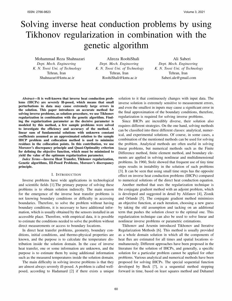
Fig. 5. The error in the collocation points on the boundary t = 0 for n = 54,f = 54, and at different noise levels, a) using the Quasi -optimality criterionb) using the Morozov’s discrepancy principle.

Fig. 6. Accurate and approximate solution on the collocation points on theboundary t = 0 for n = 54, f = 54, τ = 0.1 at different noise levels usingQuasi-optimality criterion.

Fig. (7) shows the approximate solution error on all collo-cation points. In general, the error in the internal points is lessthan the boundary collocation points.

B. Validation

The exact IHCP solved in this paper has not been solved inany paper. Therefore, to verify the method, the problem studiedby Lesnic et al. [27], which they used fundamental functionsmethod using 60 collocation points and 20 guessed functions,has been solved using out algorithm. Lesnic et al. [27] assumed

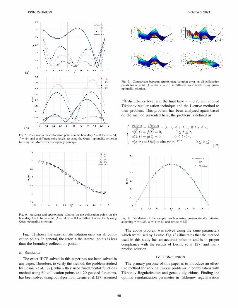
Fig. 7. Comparison between approximate solution error on all collocationpoints for n = 54, f = 54, τ = 0.1 in different noise levels using quasi-optimally criterion.

5% disturbance level and the final time τ = 0.25 and appliedTikhonov regularization technique and the L-curve method totheir problem. This problem has been analyzed again basedon the method presented here, the problem is defined as:

∂u(x,t)∂t − ∂2u(x,t)

∂x2 = 0 , 0 ≤ x ≤ 1, 0 ≤ t ≤ τ,u(0, t) = f(t) = 0, 0 ≤ t ≤ τ,u(1, t) = g(t) = 0, 0 ≤ t ≤ τ,u(x, τ) = Ω(t) = sin(πx)e−π

2τ , 0 ≤ x ≤ 1(17)

Fig. 8. Validation of the sample problem using quasi-optimally criterionassuming τ = 0.25, n = f = 60 and noise = 5% .

The above problem was solved using the same parameterswhich were used by Lesnic. Fig. (8) illustrates that the methodused in this study has an accurate solution and is in propercompliance with the results of Lesnic et al. [27] and has aprecise solution.

IV. CONCLUSION

The primary purpose of this paper is to introduce an effec-tive method for solving inverse problems in combination withTikhonov Regularization and genetic algorithms. Finding theoptimal regularization parameter in Tikhonov regularization

ISSN: 2766-9823 Volume 3, 2021

65

has been modeled to investigate the efficiency and accuracyof its application in solving sample IHCPs. Fundamentalsolutions have been used to guess estimate solution withconstant unknowns’ coefficients, and the collocation methodis applied to minimize the residue on the collocation points.

The Morozov’s discrepancy Principle and the Quasi-Optimality criterion are used to define the objective functionswhich minimizing them gives the optimal parameter. Resultsshow that the parameters of the Genetic Algorithm (likemutation rate, crossover, operator,...) should be chosen appro-priately according to the dynamic of the problem. Otherwise,the results will not be sufficiently precise. Crossover andmutation operators play the main role in minimizing andchanging the selection operator did not have any practicaleffect on minimizing the objective function. By increasing thenumber of collocation or nodal points, the condition numberof the matrix of coefficients increased, and it became severelyill-conditioned, however, if regularization applied successfully,the increase of nodal or collocated points results in lesserror in the estimated solution. The quasi-optimality criterionwas more effective at smaller final times while Morozov’sdiscrepancy principle was better at larger final times. Theobjective function of the Quasi-Optimality criterion minimizedto lower values with respect to Morozov’s objective function.Comparing the results of the proposed hybrid method pre-sented in this paper with the analytical solution and the resultsof other researchers indicates the efficiency and accuracy ofthis method in solving inverse problems.

REFERENCES

[1] Zhang B, Qi H, Ren Y, Sun S.C, Ruan L., Application of homogenouscontinuous ant colony optimization algorithm to inverse problem of onedimensional coupled radiation and conduction heat transfer, Int. J. HeatMass Transfer,66 (2013), 507—516.

[2] Hadamard, Jacques, Sur les problems aux derives partielles et leursignification physique, Princeton university bulletin. (1902), 49–52.

[3] Stolz G., Numerical solutions to an inverse problem of heat conductionfor simple shapes, J. Heat Transfer, 82 (1960), 20-–26.

[4] Alifanov O. M., Solution of an inverse problem of heat conduction byiterations methods, J. Eng. Phys. Thermophys, 26 (1974), 471-–476.

[5] Zisnik M.N, Orlande H.R.B., Inverse Heat Transfer, Taylor and Francis,New York, (2000).

[6] Tikhonov A, Arsenin V., Solutions of Ill-posed problems, Scripta Seriesin Mathematics, Winston, 1977.

[7] Beck J, Blackwell B, Clair C., Inverse Heat Conduction: Ill-Posed Prob-lems, A Wiley-Interscience Publication, John Wiley Sons Incorporated,(1985).

[8] Hensel E., Inverse theory and applications for engineers, Prentice HallAdvanced Reference Series Physical and Life Sciences, Prentice Hall,(1991).

[9] Lesnic D, Elliott L, Ingham D.B. Application of the boundary elementmethod to inverse heat conduction problems, Int. J. Heat Mass Transfer,39 (1996), 1503—1517.

[10] Blum J, Marquardt W. An optimal solution to inverse heat conductionproblems based on frequency-domain interpretation and observers, HeatTransfer Part B, 32 (1997), 453—478.

[11] SeogYeun Y, Lee, K.H, Han S.M., Smooth fitting with a method for de-termining the regularization parameter under the genetic programmingalgorithm, Information Sciences, 133, (2001) ,175–194.

[12] Keanini R.G, Ling X, Cherukuri H.P., A modified sequential functionspecification finite element-based method for parabolic inverse heatconduction problems, Comput. Mech., 36 (2005), 117-–128.

[13] Slota D. Using genetic algorithms for the determination of a heattransfer coefficient in three-phase inverse Stefan problem, Int. Commun.Heat Mass Transfer, 35 (2008), 149–156.

[14] Ajith M., Das R., Uppaluri R., Mishra S.C., Boundary Surface HeatFluxes in a Square Enclosure with an Embedded Design Element, J.Thermophys Heat Transfer, 24 (2010), 845–849.

[15] Stephany S, Becceneri J.C, Souto R.P., de Campos Velho H. F. ,Silva Neto A. J., A pre-regularization scheme for the reconstructionof a spatial dependent scattering albedo using a hybrid ant colonyoptimization implementation, Appl. Math. Modell., 34 (2010), 561–572.

[16] Singh K., Das R, Kundu B., Approximate Analytical Method for PorousStepped Fins with Temperature-Dependent Heat Transfer Parameters, J.Thermophys Heat Transfer, 30 (2016), 661–672.

[17] Chen W.L, Yang Y.C., Inverse prediction of frictional heat flux andtemperature in sliding contact with a protective strip by iterativeregularization method, Appl. Math. Modell, 35 (2011),2874–2886.

[18] Shahnazari M, Samandari-Masouleh L, Emami S. Equipment capacityoptimization of an educational building’s CCHP system by geneticalgorithm and sensitivity analysis, Energy Equipment and Systems, 5(2017), 375–387.

[19] Liu D, Yan J, Sen, K., On the treatment of non-optimal regularizationparameter influence on temperature distribution reconstruction accuracyin participating medium, Int. J. Heat Mass Transfer, 55 (2012), 1553–1560.

[20] Pourgholi R, Dana H, Tabasi S. H., Solving an inverse heat conductionproblem using genetic algorithm: Sequential and multi-core paralleliza-tion approach, Appl. Math. Modell, 48 (2014),1948–1958.

[21] Udayraj, K. Mulani, P. Taduktal, A. Das, R. Alagirusamyc, Performanceanalysis and feasibility study of ant colony optimization, particle swarmoptimization and cuckoo search algorithms for inverse heat transferproblems, Int. J. Heat Mass Transfer, 89, (2015) 359–378.

[22] Shahnazari M.R, Ahmadi Z, Masooleh L.S., Perturbation analysis ofheat transfer and a novel method for changing the third kind boundarycondition into the first kind. J. Porous Media, 20 (2017), 449-–460.

[23] Sun Sh, Qi H, Zhao F., Ruan L, Li B., Inverse geometry design of two-dimensional complex radiative enclosures using krill herd optimizationalgorithm, Appl. Therm. Eng., 98 (2016) 1104–1115.

[24] Morozov V.A. The principle of discrepancy in the solution of incon-sistent equations by Tikhonov regularization method, Zhurnal Vychisli-tel’noy matematiky i matematicheskoy. Siki., 13(5) (1973) (in Russian).

[25] Phillips D.L., A technique for the numerical solution of certain integralequation of the first kind, J. ACM . 9 (1962), 84–97.

[26] Bakushinskii A. B., Remarks on Choosing a Regularization parameterusing the quasi-optimality and ratio criterion, Comput. Math. Math.Phys., 24(4) (1984) 181–182.

[27] Lesnic, D., Elliott, L. and Ingham, D.B., An iterative boundary elementmethod for solving the backward heat conduction problem using anelliptic approximation, Inverse Prob. Eng., 6(4) (2007) 255—279.

ISSN: 2766-9823 Volume 3, 2021

66