Engineering Applications of Computational Fluid Mechanics Vol. 8, No. 2, pp. 299–307 (2014) 299 INVESTIGATION OF UNSTEADY FLOWS AND NOISE IN ROTOR- STATOR INTERACTION WITH ADJUSTABLE LEAN VANE Haijian Liu*, Hua Ouyang*^, Yadong Wu**, Jie Tian* and Zhaohui Du* *School of Mechanical Engineering, Shanghai Jiao Tong University, Shanghai 200240, China **School of Aeronautics and Astronautics, Shanghai Jiao Tong University, Shanghai 200240, China ^E-Mail: [email protected] (Corresponding Author) ABSTRACT: The paper is a study of the noise reduction effects of the stator lean angle. Firstly, a numerical study has been carried out to investigate the unsteady characteristics of the flow induced by the rotor-stator interaction. To obtain the rotor‟s wake, the distribution of the RMS pressure and the pressure disturbance coefficient, the compressor with an adjustable stator lean angle has been numerically studied. Then the compressor was experimentally tested at 11 different lean angles to obtain the free field noise spectra. Both the unsteady flow property and noise characteristics are discussed on the basis of the Computational Fluid Dynamics (CFD) results. The results indicate that (1) the pressure fluctuation of stator is the main source of the interaction noise; (2) the phase of rotor‟s wake can be tuned by the lean angle of the stator; (3) the distribution of the first harmonic of tone noise decides the distribution of total Sound Pressure level (SPL); and (4) stator with positive lean angle has better noise reduction than negative one and the lean angle should exceed 10° for better noise reduction. Keywords: rotor-stator interaction, tone noise, unsteady simulation 1. INTRODUCTION With the development of high bypass ratio of the turbofan, it is important to satisfy passengers‟ demand for comfort and quiet of the flight, and the reduction of noise of the aeroengine becomes more and more crucial. The decrease of the rotor- stator interaction noise requires profound understanding of the complex unsteady flow field. There are two types of noise in turbofan: tone and broadband noise. The interaction between rotor and stator makes the flow field highly unstable. It will also make strong tone noise because the flow field alters periodically and the most prominent component of interaction noise is tone noise. Stator lean and sweep have been suggested as one mechanism to reduce the interaction noise. Blade lean angle is the circumferential displacement of the blade stacking line relative to the radial direction; it assumed that the lean angle is positive when the blade is leaned in the direction of rotor rotation. It has been proved that the Sound Pressure Level (SPL) of the first Blade Passing Frequency (BPF) tone and the total noise are decreased by the proper combination of the lean and sweep angle of stator by NASA (Envia and Nallasamy, 1999, Woodward et al., 2001 and 2002). Their research had shown that the maximum noise decrease of the tone noise was about 6 dB. The tone noise level of modified stators was significantly reduced beyond what was achieved by simply relocating the conventional radial stator to the downstream location. The broadband noise level was also reduced by the swept stators. In order to obtain the details of flow field for noise prediction, both numerical simulation and experiment techniques should be adopted. It is impossible to capture all characteristics of the flow field by experimental methods, and the numerical calculation becomes an important technique to obtain the details of it. Ferrecchia et al. (2003) utilized numerical simulation to capture the development process of rotor wakes. The noise source was separated into several components through numerical methods by Nark et al. (2009) and Peters and Spakovszky (2012), and noise prediction was carried out. Cooper and Peake (2006) used the wake evolution and the quasi-3D strip method to develop an asymptotic technique and a new model for the wake interaction. For experimental research, Sentker and Riess (2000) obtained the velocity and turbulent intensity distribution of S1 and S3 surfaces in a 1.5 stage compressor. S1 is the stream surface formed by fluid particles lying on a circular arc of radius of the blade row. S3 surface is the plane of the blade row which is perpendicular to the axis of rotation. The dynamic flow field data and velocity fluctuation from the same surface between the gaps had also been captured by PIV measurement (Ottavy et al., Received: 4 Mar. 2013; Revised: 11 Dec. 2013; Accepted: 4 Feb. 2014

Welcome message from author
This document is posted to help you gain knowledge. Please leave a comment to let me know what you think about it! Share it to your friends and learn new things together.
Transcript
Engineering Applications of Computational Fluid Mechanics Vol. 8, No. 2, pp. 299–307 (2014)
299
INVESTIGATION OF UNSTEADY FLOWS AND NOISE IN ROTOR-
STATOR INTERACTION WITH ADJUSTABLE LEAN VANE
Haijian Liu*, Hua Ouyang*^, Yadong Wu**, Jie Tian* and Zhaohui Du*
*School of Mechanical Engineering, Shanghai Jiao Tong University, Shanghai 200240, China
**School of Aeronautics and Astronautics, Shanghai Jiao Tong University, Shanghai 200240, China
^E-Mail: [email protected] (Corresponding Author)
ABSTRACT: The paper is a study of the noise reduction effects of the stator lean angle. Firstly, a numerical study
has been carried out to investigate the unsteady characteristics of the flow induced by the rotor-stator interaction. To
obtain the rotor‟s wake, the distribution of the RMS pressure and the pressure disturbance coefficient, the
compressor with an adjustable stator lean angle has been numerically studied. Then the compressor was
experimentally tested at 11 different lean angles to obtain the free field noise spectra. Both the unsteady flow
property and noise characteristics are discussed on the basis of the Computational Fluid Dynamics (CFD) results.
The results indicate that (1) the pressure fluctuation of stator is the main source of the interaction noise; (2) the phase
of rotor‟s wake can be tuned by the lean angle of the stator; (3) the distribution of the first harmonic of tone noise
decides the distribution of total Sound Pressure level (SPL); and (4) stator with positive lean angle has better noise
reduction than negative one and the lean angle should exceed 10° for better noise reduction.
Keywords: rotor-stator interaction, tone noise, unsteady simulation
1. INTRODUCTION
With the development of high bypass ratio of the
turbofan, it is important to satisfy passengers‟
demand for comfort and quiet of the flight, and
the reduction of noise of the aeroengine becomes
more and more crucial. The decrease of the rotor-
stator interaction noise requires profound
understanding of the complex unsteady flow field.
There are two types of noise in turbofan: tone and
broadband noise. The interaction between rotor
and stator makes the flow field highly unstable. It
will also make strong tone noise because the flow
field alters periodically and the most prominent
component of interaction noise is tone noise.
Stator lean and sweep have been suggested as one
mechanism to reduce the interaction noise. Blade
lean angle is the circumferential displacement of
the blade stacking line relative to the radial
direction; it assumed that the lean angle is
positive when the blade is leaned in the direction
of rotor rotation.
It has been proved that the Sound Pressure Level
(SPL) of the first Blade Passing Frequency (BPF)
tone and the total noise are decreased by the
proper combination of the lean and sweep angle
of stator by NASA (Envia and Nallasamy, 1999,
Woodward et al., 2001 and 2002). Their research
had shown that the maximum noise decrease of
the tone noise was about 6 dB. The tone noise
level of modified stators was significantly
reduced beyond what was achieved by simply
relocating the conventional radial stator to the
downstream location. The broadband noise level
was also reduced by the swept stators. In order to
obtain the details of flow field for noise
prediction, both numerical simulation and
experiment techniques should be adopted. It is
impossible to capture all characteristics of the
flow field by experimental methods, and the
numerical calculation becomes an important
technique to obtain the details of it. Ferrecchia et
al. (2003) utilized numerical simulation to capture
the development process of rotor wakes. The
noise source was separated into several
components through numerical methods by Nark
et al. (2009) and Peters and Spakovszky (2012),
and noise prediction was carried out. Cooper and
Peake (2006) used the wake evolution and the
quasi-3D strip method to develop an asymptotic
technique and a new model for the wake
interaction. For experimental research, Sentker
and Riess (2000) obtained the velocity and
turbulent intensity distribution of S1 and S3
surfaces in a 1.5 stage compressor. S1 is the
stream surface formed by fluid particles lying on
a circular arc of radius of the blade row. S3
surface is the plane of the blade row which is
perpendicular to the axis of rotation. The dynamic
flow field data and velocity fluctuation from the
same surface between the gaps had also been
captured by PIV measurement (Ottavy et al.,
Received: 4 Mar. 2013; Revised: 11 Dec. 2013; Accepted: 4 Feb. 2014
Engineering Applications of Computational Fluid Mechanics Vol. 8, No. 2 (2014)
300
2003) and hot wire anemometer (Oro et al.,
2011). The spectra of pressure fluctuation on the
blade surface had been measured by pressure
sensors, which were buried beneath the surface of
the rotor and stator (Wang et al., 2006).
The literature about the rotor-stator interaction
indicates that previous researches were aimed at
unsteady effect of flow field and noise prediction,
but less attention was paid to the combination of
unsteady property of flow field with noise
generation. The flow field and noise
characteristics of a 1.5 stage compressor with an
adjustable stator are investigated in this paper.
Detailed discussion is carried out based on CFD
studies and the acoustic measurement.
Firstly, a compressor with three stator lean angles
has been employed for numerical studies to obtain
the pattern of rotor‟s wake, the RMS pressure
fluctuation and the disturbance coefficient
distribution of blade surface. Then the compressor
is acoustically tested to capture the free field
noise spectra. A comparison is made between
results of numerical calculation and aeroacoustic
test.
Table 1 Parameters of compressor.
Parameters Number
Rotation speed n(rpm) 3000
Hub ratio 0.7
Vane : rotor : stator 13:21:21
Design pressure rise (pa) 1800
Mass flow (kg/s) 4.9
Stator blade lean angle ξ(°) (-25~25)
Rotor tip speed(m/s) 94.25
Rotor solidity 1.598
Stator solidity 1.548
2. COMPRESSOR
A 1.5 stage low-speed axial flow compressor has
been employed to study the flow field and
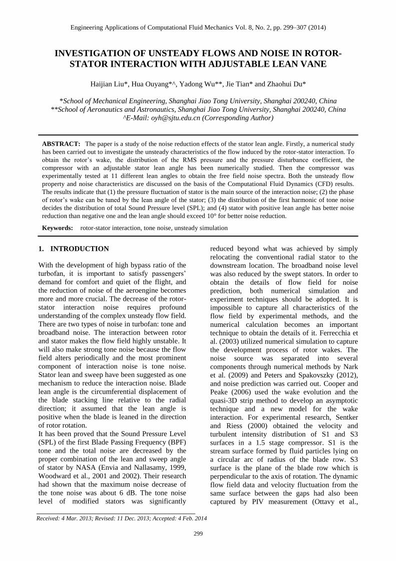
interaction noise. Fig. 1 shows the sketch of the
test rig, and the main parameters of the
compressor are listed in Table 1. There is an inlet
bellmouth and one throttle installed at the inlet
and outlet of the compressor, and the mass flow
can be tuned by the position of the throttle.
The compressor has an adjustable stator, whose
blades can be leaned positively or negatively
relative to the center. The lean is defined by the
angle ξ, and it is positive in the direction of rotor
rotation as shown in Fig. 2. The lean angle of
stator can be altered from -25° to 25° with 1°
resolution by the handle fixed at the shroud.
Fig. 1 Sketch of test rig.
(a) Sketch of lean blade driving mechnism
(b) Photos of stator
Fig. 2 Definition of lean angle ξ.
0.30 0.35 0.40 0.45 0.50 0.55 0.600.40
0.45
0.50
0.55
0.60
0.65
0.70
N25
S0
P25
(a) Eefficiency versus mass flow rate
0.30 0.35 0.40 0.45 0.50 0.55 0.601.004
1.006
1.008
1.010
1.012
1.014
1.016
1.018
N25
S0
P25
(b) Total pressure ratio versus mass flow rate
Fig. 3 Experimental performance of compressor for
cases N25, S0 and P25.
Engineering Applications of Computational Fluid Mechanics Vol. 8, No. 2 (2014)
301
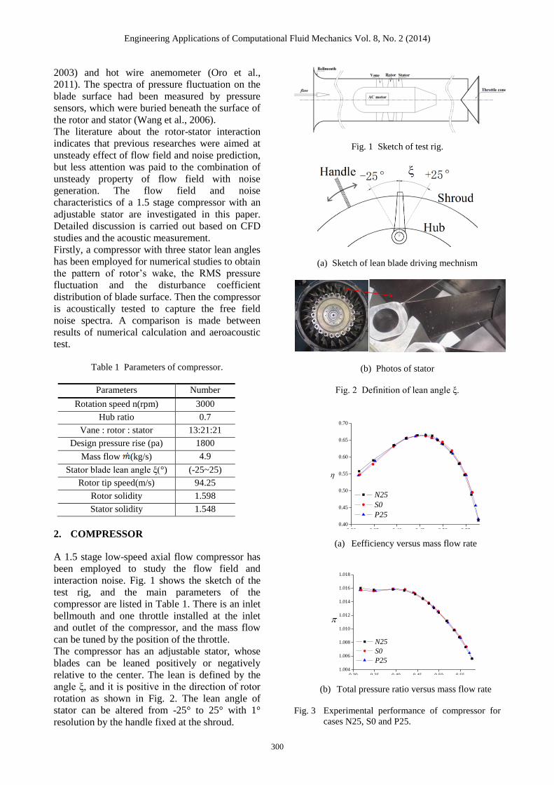
Fig. 3 is the experimental test results of the
aerodynamic performance of the compressor with
25°, 0° and -25° stator lean angles named cases
P25, S0 and N25, respectively. The prefix „N‟
means that the stator has negative lean angle,
while prefix „P‟ means positive lean angle. It is
obvious that cases P25 and N25 have little
difference in efficiency and total pressure ratio
compared with the baseline case S0.
3. NUMERICAL STUDY
3.1 CFD setup
The compressor has 13 vane blades, 21 rotor
blades and 21 stator blades. In order to avoid full
channel computation and to reduce the
consumption of the computational resources, the
number of inlet vanes has been tuned to 14 and
the chord length of blade has been reduced at the
same time to keep the solidity. The ratios between
the 1.5 stage compressor components become
vane: rotor: stator = 2:3:3. Three lean angles -25°,
0°, and 25° have been adopted for numerical
studies, which are correspondingly cases N25, S0
and P25.
The numerical simulations were undertaken with
the commercial computational fluid dynamics
code FINE/Turbo of NUMECA, which has been
extensively used in the turbomachinery industry.
Its continuous development over the years has
extended its versatility to a number of aero-
engines design applications. Spalart-Allmaras
turbulence model is used to predict the turbulence
viscosity in the flow fields because of its excellent
stability. Central spatial discretization scheme is
adopted and domain scaling method is utilized to
deal with the rotor-stator interface. The inlet and
outlet boundary are set to total pressure 101325
Pa and 102426 Pa, respectively, to make sure the
mass flow is 4.9 kg/s for every lean angle. At the
beginning of unsteady simulation, steady
simulation results are employed as initial flow
field. The dual time stepping technique is adopted
for the unsteady calculations, and the single rotor
passage is divided into 64 time steps and the
unsteady time step size is 1.488×10⁻⁵
s. Each time
step contains 40 inner subiterations. Enhanced
implicitness method is utilized and the CFL
number is set to 3 to obtain a good computation
accuracy and affordable convergence time.
To assess the uncertainty of grid number, a spatial
refinement mesh study has been carried out by
evaluating three meshes with total cell numbers of
approximately 2.9, 3.8, and 4.9 million. The grid
independence convergence study was limited to
steady computations to diminish the need of
resources. Table 2 shows the validation of the
grids independence sensitivity. The grid of
medium refinement with 3.8 million cells has
been adopted in the present work as it is a good
compromise between accuracy and time cost. The
compressor model for numerical calculation has 8
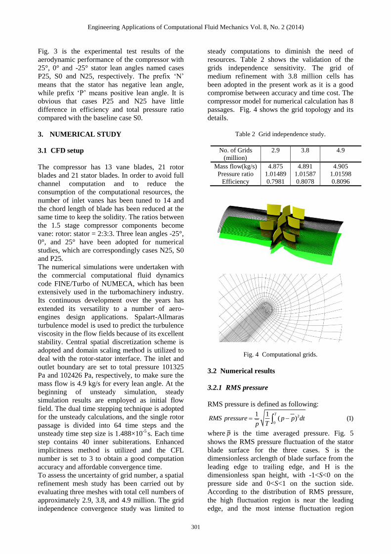
passages. Fig. 4 shows the grid topology and its
details.
Table 2 Grid independence study.
No. of Grids
(million)
2.9 3.8 4.9
Mass flow(kg/s) 4.875 4.891 4.905
Pressure ratio 1.01489 1.01587 1.01598
Efficiency 0.7981 0.8078 0.8096
Fig. 4 Computational grids.
3.2 Numerical results
3.2.1 RMS pressure
RMS pressure is defined as following:
2
0
1 1 ( ) (1)
T
RMS pressure p p dtTp
where is the time averaged pressure. Fig. 5
shows the RMS pressure fluctuation of the stator
blade surface for the three cases. S is the
dimensionless arclength of blade surface from the
leading edge to trailing edge, and H is the
dimensionless span height, with -1<S<0 on the
pressure side and 0<S<1 on the suction side.
According to the distribution of RMS pressure,
the high fluctuation region is near the leading
edge, and the most intense fluctuation region
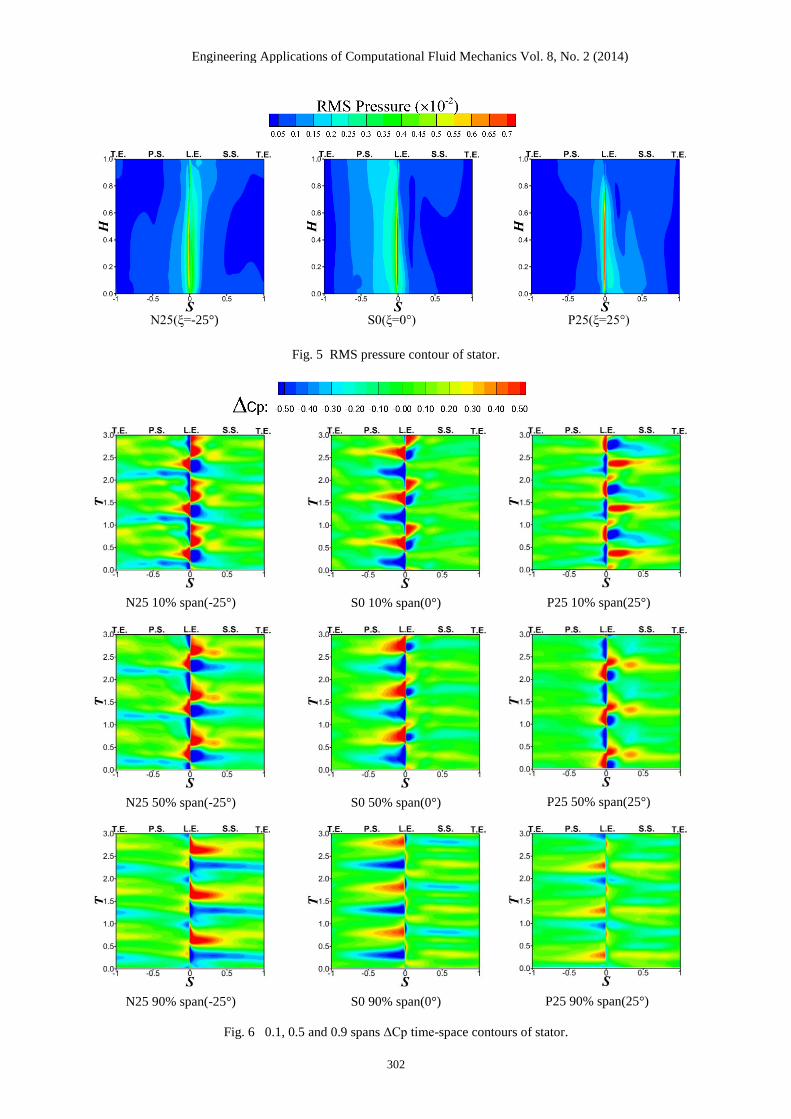
Engineering Applications of Computational Fluid Mechanics Vol. 8, No. 2, pp. 299–307 (2014)
302
N25(ξ=-25°)
S0(ξ=0°)
P25(ξ=25°)
Fig. 5 RMS pressure contour of stator.
N25 10% span(-25°)
S0 10% span(0°)
P25 10% span(25°)
N25 50% span(-25°)
S0 50% span(0°)
P25 50% span(25°)
N25 90% span(-25°)
S0 90% span(0°)
P25 90% span(25°)
Fig. 6 0.1, 0.5 and 0.9 spans ΔCp time-space contours of stator.
Engineering Applications of Computational Fluid Mechanics Vol. 8, No. 2 (2014)
Engineering Applications of Computational Fluid Mechanics Vol. 8, No. 2, pp. 299–307 (2014)
303
locates at pressure side from the root to 80%
height near the leading edge. The flow angle gets
increased when the wakes sweep from the stator‟s
leading edge, which increases the pressure on the
pressure side; and pressure decreases on the
suction side with a positive attack angle at the
same time. All the reasons above cause the
pressure fluctuating intensely near the leading
edge. Compared with baseline case S0, the range
of RMS pressure fluctuations of cases N25 and
P25 are smaller, especially at the pressure side of
case P25. The lean negative blade has more
constraint than positive and straight one for the
radial flow on pressure side, and the radial flow
on the pressure side of P25 is weaker than that of
cases S0 and N25.
3.2.2 Pressure disturbance coefficient ΔCp
The pressure disturbance coefficient ΔCp is
defined as follows:
0
2
0
(2)
( ) / (0.5 ) (3)
Cp Cp Cp
Cp p p v
where Cp is the pressure coefficient, and Cp0
presents the time averaged pressure coefficient. p0
and 0.5ρv2 are the inlet total pressure and dynamic
pressure at stator‟s inlet, respectively.
Fig. 6 shows the pressure disturbance coefficient
time-space distribution at 10%(root), 50%(middle
span), and 90%(top) of span height. S is the
dimensionless arclength of blade surface from the
leading edge, and T is time period. The maximum
pressure disturbance coefficient is near the
leading edge, the high pressure and low pressure
area distribute alternately with time period. The
lean negative blade(case N25) has more constraint
for radial flow at pressure side than straight and
positive ones, so its ΔCp varies more intensely
and widely on pressure side at the root region.
Correspondingly, the ΔCp of case P25 has more
intense fluctuation at suction side of root region
than others. At the middle span 50% and top 90%
region, the lean positive stator blade(case P25)
has minimum pressure disturbance coefficient.
Compared with case N25 and S0, the range and
the intensity of ΔCp of case P25 are minimum,
especially at the pressure side.
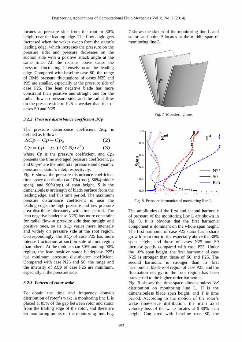
3.2.3 Pattern of rotor wake
To obtain the time and frequency domain
distribution of rotor‟s wake, a monitoring line L is
placed at 85% of the gap between rotor and stator
from the trailing edge of the rotor, and there are
65 monitoring points on the monitoring line. Fig.
7 shows the sketch of the monitoring line L and
stator, and point P locates at the middle span of
monitoring line L.
P
Fig. 7 Monitoring line.
0 20 40 60 80 100 120 140 1600.0
0.2
0.4
0.6
0.8
1.0
N25
S0
P25
Sp
an
Amplitude
1st
2nd
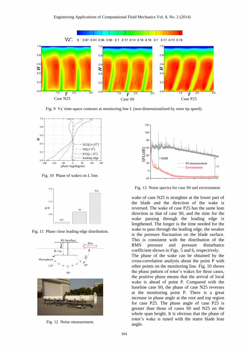
Fig. 8 Pressure harmonics of monitoring line L.
The amplitudes of the first and second harmonic
of pressure of the monitoring line L are shown in
Fig. 8. It is obvious that the first harmonic
component is dominant on the whole span height.
The first harmonic of case P25 stator has a sharp
growth from root-to-tip, especially above the 30%
span height; and those of cases N25 and S0
increase gently compared with case P25. Under
the 10% span height, the first harmonic of case
N25 is stronger than those of S0 and P25. The
second harmonic is stronger than its first
harmonic at blade root region of case P25, and the
fluctuation energy in the root region has been
transferred to the higher-order harmonics.
Fig. 9 shows the time-space dimensionless Vz′
distribution on monitoring line L. H is the
dimensionless blade span height, and T is time
period. According to the motion of the rotor‟s
wake time-space distribution, the main axial
velocity loss of the wake locates at 0-80% span
height. Compared with baseline case S0, the
Engineering Applications of Computational Fluid Mechanics Vol. 8, No. 2 (2014)
Engineering Applications of Computational Fluid Mechanics Vol. 8, No. 2, pp. 299–307 (2014)
304
Case N25 Case S0 Case P25
Fig. 9 Vz’ time-space contours at monitoring line L (non-dimensionalized by rotor tip speed).
-180 -120 -60 0 60 120 1800.0
0.2
0.4
0.6
0.8
1.0
N25(=-25o)
S0(= 0o)
P25(25)
leading edge
H
phase lag(degree)
Fig. 10 Phase of wakes on L line.
0.00
0.06
0.12
0.18
N25
S0pcle
P25
Fig. 11 Phase close leading edge distribution.
flow
Fig. 12 Noise measurement.
0 2000 4000 6000 8000 10000-20
0
20
40
60
80
100
120
>30dB
S0 measurement
Environment
SP
L(d
B)
f(Hz)
>30dB
Fig. 13 Noise spectra for case S0 and environment.
wake of case N25 is straighter at the lower part of
the blade and the direction of the wake is
reversed. The wake of case P25 has the same lean
direction as that of case S0, and the time for the
wake passing through the leading edge is
lengthened. The longer is the time needed for the
wake to pass through the leading edge, the weaker
is the pressure fluctuation on the blade surface.
This is consistent with the distribution of the
RMS pressure and pressure disturbance
coefficient shown in Figs. 5 and 6, respectively.
The phase of the wake can be obtained by the
cross-correlation analysis about the point P with
other points on the monitoring line. Fig. 10 shows
the phase pattern of rotor‟s wakes for three cases,
the positive phase means that the arrival of local
wake is ahead of point P. Compared with the
baseline case S0, the phase of case N25 reverses
at the monitoring point P. There is a great
increase in phase angle at the root and top region
for case P25. The phase angle of case P25 is
greater than those of cases S0 and N25 on the
whole span height. It is obvious that the phase of
rotor‟s wake is tuned with the stator blade lean
angle.
Engineering Applications of Computational Fluid Mechanics Vol. 8, No. 2 (2014)
Engineering Applications of Computational Fluid Mechanics Vol. 8, No. 2, pp. 299–307 (2014)
305
_mic position
_le
an
angle
45 60 75 90 105 120 135-25
-20
-15
-10
-5
0
5
10
15
20
2597 98 99 100 101 102 103 104 105 106 107 108 109 110 111
SPL_dB(A)
(a) total noise SPL (b) tone noise SPL
(c) broadband noise SPL (d) 1st BPF SPL
Fig. 14 Contour of total, tone, broadband and 1st BPF SPL dB(A).
(a) αtone_total (b) α1st_total
Fig. 15 Ratio of tone and 1st BPF noise.
In order to evaluate the phase lag on whole span
height, phase skewing parameter Phase Close
Leading Edge (pcle) is adopted and defined as
following:
1(3)
2
top
hubpcle phase lag dh
The pcle is the phase skewing distance of the wake with stator leading edge, and pcle = 0 means
the stator leading edge. Fig. 11 is the phase
skewing parameter pcle of three cases. The
distribution of pcle shows that case N25 has the
minimum phase skewing control, and the rotor‟s
_mic position
_le
an
angle
45 60 75 90 105 120 135-25
-20
-15
-10
-5
0
5
10
15
20
250.25 0.3 0.35 0.4 0.45 0.5 0.55 0.6 0.65 0.7 0.75 0.8 0.85
tone_total
_mic position
_le
an
angle
45 60 75 90 105 120 135-25
-20
-15
-10
-5
0
5
10
15
20
250.05 0.1 0.15 0.2 0.25 0.3 0.35 0.4 0.45 0.5
1st_total
_mic position
_le
an
angle
45 60 75 90 105 120 135-25
-20
-15
-10
-5
0
5
10
15
20
2597 98 99 100 101 102 103 104 105 106 107 108 109 110 111
SPL_dB(A)
_mic position
_le
an
angle
45 60 75 90 105 120 135-25
-20
-15
-10
-5
0
5
10
15
20
2597 98 99 100 101 102 103 104 105 106 107 108 109 110 111
SPL_dB(A)
_mic position
_le
an
angle
45 60 75 90 105 120 135-25
-20
-15
-10
-5
0
5
10
15
20
2597 98 99 100 101 102 103 104 105 106 107 108 109 110 111
SPL_dB(A)
_mic position
_le
an
angle
45 60 75 90 105 120 135-25
-20
-15
-10
-5
0
5
10
15
20
2597 98 99 100 101 102 103 104 105 106 107 108 109 110 111
SPL_dB(A)
Engineering Applications of Computational Fluid Mechanics Vol. 8, No. 2 (2014)
Engineering Applications of Computational Fluid Mechanics Vol. 8, No. 2 (2014)
306
wakes of case P25 has the maximum phase lag.
4 AEROACOUSTIC EXPERIMENT
4.1 Setup
Due to the length of the compressor, the acoustic
test was carried out outside of the laboratory. Fig.
12 presents the aeroacoustic test configuration.
The noise spectra were measured by the B&K
4189 microphones with 0.2 dB uncertainty; the
output signals were received by NI PXI
1033&4472 multichannel data acquisition system.
Seven microphones were fixed around R=1m
circle from θ=45° to 135° by 15° interval, and the
center of the microphones was the interface of the
rotor and stator. The microphones and the axis of
the compressor were in the same measuring plane
parallel with the ground, and the distance of
measurement plane to the ground was 1.2 m. The
evaluation about the outside environment had also
been carried out to make sure that the
environment was satisfactory for the noise
measurements. The total sound pressure level
(SPL) of the 1m circle was at least 5 dB(A) higher
than the 2m circle when the compressor was
running, and it was accorded with the noise
degression. The environmental noise was about
42-44 dB(A) when the tests were carried out at
midnight. Typically the environmental noise was
30 dB less than the measurement as shown in Fig.
13, and the effect of environmental noise could be
neglected.
The downstream stator lean angle ξ was altered
from -25° to 25° by 5° interval, repeated 7 times
for each case.
4.2 Experiment result
The tone noise (BPF and its harmonics) and
broadband noise were separated from the noise
spectra, and the SPL measurement results for all
components are shown at Fig. 14, where θ is the
position of microphone, and ξ is the stator blade
lean angle. The SPL of the broadband component
is about 102.9-103.9 dB for all cases; the tone
noise is maximum when the lean angle ξ is 0°.
Compared with the baseline case S0, lean positive
stator has better noise reduction than lean
negative one. Fig. 14d shows the 1st harmonic of
the tone noise and it has the same distribution as
the tone and total SPL distributions. The different
distribution of the 1st BPF harmonic leads to the
different total and tone noise SPL distributions. It
is obvious that the SPL of total, tone, and 1st BPF
is stronger at the angle of |ξ|<10°. The tone noise
SPL is decreased when the lean angle |ξ|>10°, and
the noise reduction amplitude of lean negative
angle (ξ<-10°) is smaller than that of lean positive
angle (ξ>10°).
The proportion of the SPL b in the total SPL c is
defined as follows: 0.1
0.1( )
_ 0.1
1010 (4)
10
bb c
b c c
Fig. 15a shows the proportion of tone noise SPL
in total SPL αtone_total. The αtone_total is larger than
50% in almost the whole range of |ξ|<10°, and the
αtone_total exceeds 70% when the lean angle is 0°.
Fig. 15b is the proportion distribution of the 1st
BPF in total SPL α1st_total. The α1st_total can reach up
to 50% in |ξ|<10° region and decrease to 30% and
even lower when |ξ|>10°. According to the
analysis, the 1st BPF of tone noise is reduced by
the technique of adjusting the stator‟s lean blade.
The lean positive stator has more noise reduction
than lean negative one, and the lean angle should
exceed 10° for better noise reduction.
5 CONCLUSIONS
Three stator blade lean angles have been
employed for the rotor-stator interaction noise
study. The numerical study reveals the pressure
fluctuation on the stator and the phase skewing of
rotor wakes. The compressor with a series stator
lean angle has also been investigated
experimentally through acoustic measurements.
Both numerical calculations and acoustic
measurements results show that:
1. The leading edge region is the main pressure
fluctuations zone. The first harmonic of the
wake is greater than the other harmonics, and
the dramatic change occurred for case P25
from the blade root-to-tip. It has also been
proved that the first harmonic is the main
component for total SPL in the acoustic
measurement.
2. Compared with case S0, the phase of wake of
case N25 reverses, and the phase of wake of
case P25 increases. The adjustment for the
wake‟s phase of case P25 has better effect
than those of N25 and S0, and it is consistent
with noise test result.
3. The downstream stator lean angle has little
effect on the aerodynamic performance for
the compressor at low speed. The tone and 1st
harmonic of SPL distribution show that the
tone noise is determinant for total SPL. The
lean positive stator has better effect than lean
negative. And the lean angle of the stator
should exceed 10° for better noise reduction.
Engineering Applications of Computational Fluid Mechanics Vol. 8, No. 2 (2014)
307
ACKNOWLEDGEMENTS
This work has benefited from the generous
support of National Natural Science Foundation
of China under grant Nos. 11202132 and
51306110. The authors would also like to express
their appreciation of “2011 Aero-Engine
collaborative Innovation Plan” for its support.
NOMENCLATURE
Cp = Pressure coefficient
Cp0 = Time average pressure coefficient
H = Dimensionless span height
m = Mass flow, kg/s
p = Static pressure, Pa
p = Time average pressure, Pa
S = Dimensionless curve length
t = Time, s
T = Time period, s
R = Test radius of microphone, m
Vz′ = Dimensionless axial velocity
ΔCp = Pressure disturbance coefficient
αb_c = Ratio of sound pressure
ρ = Density, kg/m3
ξ = Stator lean angle, °
θ = Microphone position, °
φ = Mass flow rate
π = Total pressure ratio
η = Efficiency
REFERENCES
1. Cooper AJ, Peake N (2006). Rotor-stator
interaction noise in swirling flow : Stator
sweep and lean effects. AIAA Journal 44(5):
981-991.
2. Envia E, Nallasamy M (1999). Design
selection and analysis of a swept and leaned
stator concept. Journal of Sound and
Vibration 228(4): 793-836.
3. Ferrecchia A, Dawes W, Dhanasekaran PC
(2003). Compressor rotor wakes and tone
noise study. 9th AIAA/CEAS Aeroacoustics
Conference and Exhibit, May 12-14, Hilton
Head, SC, USA. AIAA-2003-3328.
4. Nark DM, Envia E, Burley CL (2009). Fan
noise prediction with applications to aircraft
system noise assessment. AIAA 2009-3291.
5. Oro JF, Diaz KA, Morros CS, et al. (2011).
Numerical simulation of the unsteady stator-
rotor interaction in a low-speed axial fan
including experimental validation.
International Journal of Numerical Methods
for Heat and Fluid Flow 21(2): 168.
6. Ottavy X, Trébinjac I, Vouillarmet A, et al.
(2003). Laser measurements in high speed
compressors for rotor-stator interaction
analysis. Journal of Thermal Science 12(4):
310.
7. Peters A, Spakovszky ZS (2012). Rotor
interaction noise in counter-rotating propfan
propulsion systems. Journal of
Turbomachinery 134(1): 011002.
8. Sentker A, Riess W (2000). Experimental
investigation of turbulent wake–blade
interaction in axial compressors. International
Journal of Heat and Fluid Flow 21(3): 285-
290.
9. Wang YF, Hu J, Luo BN, Li CP (2006).
Effects of the upstream blade wakes on the
spectrum of rotor blade unsteady surface
pressure. Journal of Aerospace Power 21(4):
693-699.
10. Woodward RP, Elliott DM, Hughes CE,
Berton JJ (2001). Benefits of swept-and-
leaned stators for fan noise reduction. Journal
of Aircraft 38(6): 1130-1138.
11. Woodward RP, Gazzaniga JA, Bartos LJ,
Hughes CE (2002). Acoustic benefits of stator
sweep and lean for a high tip speed fan. 40th
AIAA Aerospace Sciences Meeting and
Exhibit, January 14-17, Reno, NV, USA.
AIAA-2002-1034.
Related Documents