Investigation and Implementation of an Eigensolver Method

Investigation and Implementationof an Eigensolver Method

Jorge Moreira

August 24, 2014

Abstract

The Lánczos method is an iterative method used to find the eigenvalues and the eigen-vectors of a matrix. The aim of this dissertation was to implement an eigensolver onparallel architectures that resort to the Lánczos algorithm. The method creates a tridi-agonal matrix that needs to be solved with a tridiagonal solver from a software library,such as LAPACK or ScaLAPACK. In order to investigate its behaviour, the parallelScaLAPACK solver was tested with varying numbers of processes per MPI communi-cators, ranging from 2 to 384. As a result, a new approach was devised to optimise theperformance of the solver in parallel that employs different configurations of processes.The results have demonstrated that swapping sub-communicators slightly improves theperformance of the solvers for low iteration counts in the range utilised. This suggeststhat the same pattern of behaviour intensifies given a wider range of iterations and muchhigher numbers of processes.

Contents

1 Introduction 11.1 Tasks outline . . . . . . . . . . . . . . . . . . . . . . . . . . . . . . . 21.2 Motivation . . . . . . . . . . . . . . . . . . . . . . . . . . . . . . . . . 21.3 Thesis outline . . . . . . . . . . . . . . . . . . . . . . . . . . . . . . . 21.4 Deviation from the original workplan . . . . . . . . . . . . . . . . . . 3

2 Background 42.1 Mathematical Background . . . . . . . . . . . . . . . . . . . . . . . . 4

2.1.1 Eigenvalues and eigenvectors . . . . . . . . . . . . . . . . . . 42.1.2 Direct and iterative methods . . . . . . . . . . . . . . . . . . . 42.1.3 Normalisation . . . . . . . . . . . . . . . . . . . . . . . . . . . 52.1.4 The power method . . . . . . . . . . . . . . . . . . . . . . . . 52.1.5 The Lánczos algorithm . . . . . . . . . . . . . . . . . . . . . . 62.1.6 Tridiagonalisation and tridiagonal solver . . . . . . . . . . . . 8

2.2 MPI . . . . . . . . . . . . . . . . . . . . . . . . . . . . . . . . . . . . 92.2.1 MPI Communicators and sub-communicators . . . . . . . . . . 9

2.3 Numerical linear algebra libraries . . . . . . . . . . . . . . . . . . . . 102.3.1 LAPACK . . . . . . . . . . . . . . . . . . . . . . . . . . . . . 102.3.2 ScaLAPACK . . . . . . . . . . . . . . . . . . . . . . . . . . . 102.3.3 BLAS, PBLAS, BLACS . . . . . . . . . . . . . . . . . . . . . 112.3.4 BLACS context . . . . . . . . . . . . . . . . . . . . . . . . . . 12

3 Methodology 133.1 Hardware architectures . . . . . . . . . . . . . . . . . . . . . . . . . . 13

3.1.1 Morar . . . . . . . . . . . . . . . . . . . . . . . . . . . . . . . 133.1.2 ARCHER . . . . . . . . . . . . . . . . . . . . . . . . . . . . . 143.1.3 NUMA . . . . . . . . . . . . . . . . . . . . . . . . . . . . . . 14

3.2 Procedure description . . . . . . . . . . . . . . . . . . . . . . . . . . . 143.3 Implementation of a parallel power method . . . . . . . . . . . . . . . 16

3.3.1 Parallel matrix-vector multiplication . . . . . . . . . . . . . . . 183.3.2 Parallel replicated . . . . . . . . . . . . . . . . . . . . . . . . . 193.3.3 Parallel distributed . . . . . . . . . . . . . . . . . . . . . . . . 203.3.4 Conclusion . . . . . . . . . . . . . . . . . . . . . . . . . . . . 23

3.4 Serial Lánczos . . . . . . . . . . . . . . . . . . . . . . . . . . . . . . . 233.5 Parallel Lánczos . . . . . . . . . . . . . . . . . . . . . . . . . . . . . . 24

i

3.6 Parallel L2-normalisation . . . . . . . . . . . . . . . . . . . . . . . . . 263.7 Tridiagonal solvers . . . . . . . . . . . . . . . . . . . . . . . . . . . . 26

3.7.1 Implementation of a LAPACK eigensolver with DSTEV . . . . 273.7.2 ScaLAPACK . . . . . . . . . . . . . . . . . . . . . . . . . . . 283.7.3 Implementation of a ScaLAPACK eigensolver with PDSTEBZ . 283.7.4 CBLACS implementation . . . . . . . . . . . . . . . . . . . . 303.7.5 MPI sub-communicators implementation . . . . . . . . . . . . 32

3.8 Tridiagonal solvers investigation and further optimisation . . . . . . . . 343.8.1 Determination of crossover points . . . . . . . . . . . . . . . . 35

3.9 ScaLAPACK PDSTEIN eigensolver implementation . . . . . . . . . . 363.10 Process mapping and core affinity . . . . . . . . . . . . . . . . . . . . 37

4 Results and analysis 394.1 Verification with Octave . . . . . . . . . . . . . . . . . . . . . . . . . 394.2 Power method initial results . . . . . . . . . . . . . . . . . . . . . . . 404.3 Lánczos algorithm initial results . . . . . . . . . . . . . . . . . . . . . 414.4 Investigation of the BLACS contexts . . . . . . . . . . . . . . . . . . . 444.5 Tridiagonal solver optimisation . . . . . . . . . . . . . . . . . . . . . . 454.6 Mapping of sub-communicators to nodes . . . . . . . . . . . . . . . . . 494.7 MPI processes affinity . . . . . . . . . . . . . . . . . . . . . . . . . . . 53

5 Discussion and conclusions 565.1 Future work . . . . . . . . . . . . . . . . . . . . . . . . . . . . . . . . 58

Appendix A Source code A1

Appendix Appendices A1A.1 Lánczos Eigensolver . . . . . . . . . . . . . . . . . . . . . . . . . . . A1A.2 Crossovers Bash scripts . . . . . . . . . . . . . . . . . . . . . . . . . . A19A.3 Cpuset . . . . . . . . . . . . . . . . . . . . . . . . . . . . . . . . . . . A20A.4 Matlab Lánczos . . . . . . . . . . . . . . . . . . . . . . . . . . . . . . A22

6 test 26

ii

List of Figures

2.1 MPI communicators sub-division using MPI_Comm_split . . . . . . . 102.2 ScaLAPACK Software Hierarchy[5] . . . . . . . . . . . . . . . . . . . 11

3.1 Cray XC30 Intel Xeon compute node architecture [19]. . . . . . . . . . 153.2 Ring layout of 4 processors . . . . . . . . . . . . . . . . . . . . . . . . 183.3 Row-wise matrix partition over 4 processors. . . . . . . . . . . . . . . 193.4 Matrix-vector multiplication over 4 processors . . . . . . . . . . . . . . 233.5 ScaLAPACK subroutines executing over BLACS contexts with 12, 24

and 48 processors . . . . . . . . . . . . . . . . . . . . . . . . . . . . . 303.6 Intersection/crossover points inside peaks. . . . . . . . . . . . . . . . 36

4.1 Convergence of the eigenvalue found by the power method code to-wards the real dominant eigenvalue (λreal = 2304.000000) of matrix A,of size 48 × 48 during 100 iterations. . . . . . . . . . . . . . . . . . . . 42

4.2 Convergence of the residual error ||Av − λv|| towards 0 during 100 it-erations of the power method code (replicated and distributed), with amatrix A of size 48 × 48 (λreal = 2304.000000). . . . . . . . . . . . . . 42

4.3 Eigenvalues found by the parallel Lánczos method run on ARCHERwith 384 cores and a matrix of 12900 elements. . . . . . . . . . . . . . 43

4.4 ScaLAPACK tridiagonal solver performance on a total of 384 processesfor 5000 iterations. The number of processors per MPI sub-communicatorand BLACS context was modified at each run. . . . . . . . . . . . . . 46

4.5 Comparison of the times taken by the LAPACK and ScaLAPACK solverswith a total of 384 processes during 700 iterations. The ScaLAPACKsolver was executed within MPI communicators/BLACS contexts ofvarying sizes. . . . . . . . . . . . . . . . . . . . . . . . . . . . . . . . 46

4.6 Crossover points at the intersections between the timing curves obtainedrunning LAPACK serially on all the cores and ScaLAPACK in parallelwith 24 and 48 cores per sub-communicator. These points show thata different number of cores per BLACS context or MPI communicatorshould be utilised. . . . . . . . . . . . . . . . . . . . . . . . . . . . . 47

4.7 Performance obtained running ScaLAPACK within MPI communica-tors/BLACS contexts with 48, 96, 192 and 384 cores. The crossoverpoints show the intersections between the several timings curves. . . . . 47

iii

4.8 Comparison of the overall time taken by an single Lánczos iteration bythe optimised version, a version using LAPACK and by another usingscalable with BLACS contexts of 384 cores. . . . . . . . . . . . . . . . 49

4.9 Optimised version of the code with insertion of “switching” points thatswap BLACS contexts at given iterations. . . . . . . . . . . . . . . . . 50

4.10 Timings of different sections of the code of the optimised version. . . . 504.11 Proportions taken by the different parts of the code of the optimised

version. . . . . . . . . . . . . . . . . . . . . . . . . . . . . . . . . . . 514.12 Performance obtained for single instance of scalable running on 4800

cores compared with previous timings obtained with lesser cores. . . . . 514.13 Example of mapping 96 MPI processes to 4 computational nodes on

ARCHER. Each process has an affinity to core that can be modified. . . 54

iv

List of Tables

3.1 Number of processes per MPI sub-communicator with the resultingnumbers of subgroups and of ScaLAPACK instances. . . . . . . . . . 16

3.2 Vectors being swapped around processors . . . . . . . . . . . . . . . . 21

4.1 Example of the output obtained running the replicated power methodwith a small matrix of 6 elements on 2 processors on Morar. . . . . . . 41

4.2 Spurious eigenvalues found with the Lánczos algorithm run for 5000iterations with a matrix of 12900 × 12900. The dots (. . .) mean thatvalues have been omitted for clarity. Separators (lines) mean that achange occurs in the value of the real eigenvalue. . . . . . . . . . . . . 44

4.3 Iteration numbers at which a new MPI sub-communicator was startedwith a different number of processes, including the resulting numbersof subgroups and of ScaLAPACK instances. LAPACK was used forlow numbers of iterations, from iteration 0 to 215. . . . . . . . . . . . 48

4.4 Mapping of 96 MPI processes onto a BLACS layout grid of 24 pro-cesses. The dots (...) mean some that lines have been omitted for clarityand separators (lines) divide BLACS contexts. . . . . . . . . . . . . . . 52

4.5 Mapping of 96 MPI processes onto a BLACS grid layout of 48 pro-cesses. The dots (...) mean that some lines have been omitted for clarityand separators (lines) divide BLACS contexts. . . . . . . . . . . . . . . 53

4.6 Mapping of 96 MPI processes onto 4 computational nodes on ARCHER.The dots (...) mean that some lines have been omitted for clarity andseparators (lines) divide BLACS contexts. . . . . . . . . . . . . . . . . 55

6.1 Mapping of 96 MPI processes onto a BLACS grid layout of 48 pro-cesses. The dots (...) mean that some lines have been omitted for clarityand separators (lines) divide BLACS contexts. . . . . . . . . . . . . . . 26

v

Acknowledgements

The author would like to thank gratefully his project supervisor Dr. Christopher Johnsonfor his guidance and assistance on this project and also Dr. Judy Hardy for her supportduring difficult times. The author would also like to show his gratitude to his parentsfor their support.

The author gratefully acknowledge the funding sources that made this MSc possible.The tuition fees were covered by a PTAS scholarship from SAAS and a bursary fromthe School of Physics and Astronomy of the University of Edinburgh.

vi

Chapter 1

Introduction

The Lánczos method is a known algorithm to calculate eigenvalues and eigenvectors inmatrices. It has many relevant applications in Physics and Mathematics or Engineeringsuch as in vibration problems [22]. Although considered a simple method, the Lánczosmethod is a quick and accurate technique to efficiently find more than one eigenvalue oreigenvector in a matrix. By contrast, it shows a number of issues that have led to lackof interest during several decades [24].

The flaws presented by the algorithm can nonetheless be circumvented or corrected as isshown by the extensive research that exists around the subject [14]. For example, Parlettand Scott have developed a method called LANSO that introduces re-orthogonalisationto mitigate the loss of orthogonality issues presented by the Lánczos algorithm [28].Johnson and Kennedy have further refined the LANSO algorithm when studying onlypart of the matrix spectrum [21]. These are just a few works that aim to correct certainunwanted weaknesses of the Lánczos method. Some areas in the projects just men-tioned were left for improvement in future works and certainly show room for furtherinvestigation in less known aspects of the algorithm.

This project concerns the parallel implementation of the Lánczos method on supercom-puters and the detailed observation of the behaviour of the resulting application. Thecomputations that involves solving the tridiagonal matrix obtained from the Lánczositeration are the main area of interest that shows potential for improvement, namelyin the way they can be parallelised. The application of different varying layouts ofprocessors in the calls to tridiagonal LAPACK and ScaLAPACK solvers resulted in asubsequent optimisation that has enabled enhancing the performance of the whole pro-cess of finding eigenvalues and eigenvectors, especially for small numbers of iterations.This optimisation method was devised and added to the code, based on the investigationand subsequent identification of the best execution timings.

1

1.1 Tasks outline

The problems handled by this dissertation were divided into several main points. Thefollowing steps have been undertaken:

1. given a serial power method it has been adapted to run in parallel on Morar, asmall supercomputer with 128 cores;

2. the code was ported to ARCHER, a much larger supercomputer with 72,192cores, and subsequent adjustments were performed;

3. a Lánczos method was coded based on the power method code. First, sequentiallythen adapted to run in parallel on Morar;

4. the code was ported to ARCHER;

5. a process to solve the tridiagonal matrix resulting from the Lánczos computa-tion was implemented to obtain a subset of the eigenvalues, using LAPACK andScaLAPACK;

6. the performance of the tridiagonal solvers was investigated in serial and in paral-lel;

7. the code was optimised based on the previous observations;

8. the mapping of MPI processes to computational nodes was investigated.

9. a process to calculate the eigenvectors from the eigenvalues was devised;

1.2 Motivation

The initial idea underlying this project was based on Johnson and Kennedy’s paper [21]and the implementation of a Lánczos method with Chroma [13], a software package forsolving Lattice Quantum Chromodynamics problems. Since Chroma does not allow ac-ccess to lower levels of its functioning such as the communication layers, some aspectscould not be easily assessed. It was then suggested that a Lánczos implementation thatoffered greater flexibility would be more helpful in understanding some of these aspects.Hence, the need for a more flexible Lánczos code that enabled, for instance, modifyingthe number of cores allocated to the tridiagonal solvers.

1.3 Thesis outline

Chapter 2 provides the background on key notions necessary to understanding the math-ematical concepts behind the implementation of the Lánczos method. It includes very

2

brief recapitulations of eigenvectors and eigenvalues, of the power method and of theLánczos algorithm.

Chapter 3 outlines the methodology used in the serial and parallel implementations ofthe several algorithms and describes how these were further investigated. An explana-tion of the optimisation process derived from these observations follows.

Chapter 4 presents the results obtained from the previous observations and investiga-tions with graphs and tables that show data obtained with a first analysis of the out-comes.

Chapter 5 further discusses the results and concludes the work carried out in this thesis.It finalises the dissertation with some suggestions for future work that could be derivedfrom the present project.

1.4 Deviation from the original workplan

It should be noted here that a small number of tasks included in the original work-plan have been abandoned during the course of the project to concentrate on others.Originally, two different aspects of the implemented were to be considered, namely theinvestigation of the tridiagonal solvers and that of the creation of the Lánczos vectorsduring the Lánczos iteration. However, during the course of the project, after obtainingpositive results with the tridiagonal solvers in parallel, it was decided that there wasenough matter to cover with their implementation. The result was that some of theinitial steps were not undertaken, namely:

1. the investigation of different dense matrix storage schemes on ARCHER;

2. a comparison with the existing Lánczos implementation of Johnson and Kennedythat makes use of the Chroma library;

3. the investigation of the creation and of the storage of the Lánczos vectors gener-ated during the Lánczos iteration.

The current project has nonetheless focused on several aspects concerning the imple-mentation of the tridiagonal solvers in parallel.

3

Chapter 2

Background

2.1 Mathematical Background

Methods for solving eigenvalue problems are of particular significance in Physics, orPure and Applied Mathematics [22]. They are essential in the study of matrices [27].

2.1.1 Eigenvalues and eigenvectors

According to formal definitions, a complex scalar λ ∈ � is considered an eigenvalue ofan n × n complex matrix A ∈ �n×n if there is a vector v ∈ �n with v , 0 such that therelation

A · v = λv (2.1)

holds. In this case, the vector v is called the eigenvector associated with the eigenvalueλ. Λ is called the spectrum of the matrix A and consists of the set of all eigenvalues[23] [9]. An eigenvalue together with its associated eigenvector will be referred to asan eigenpair in this paper.

2.1.2 Direct and iterative methods

There are two kinds of methods for calculating eigenpairs: direct and iterative methods.Direct methods are known to always converge to the solution in a deterministic fashion,in other words, they will always get to the expected results in a known number ofiterations and are useful for dense matrices [9]. On the other hand, the computationalcost of this group of methods lies in the order of O(n3) when it comes to finding alleigenpairs.

4

By contrast, iterative methods find a subset of approximations to solutions. They areuseful for sparse matrices or algorithms involving matrix-vector multiplication [9].Common techniques involve transforming the original matrix into a simpler form orcanonical form, which in turn is easier to process in order to find eigenpairs. Thesekinds of operations are called similarity transformations. The easiest matrix to processwould logically be a diagonal matrix whose eigenvalues are its diagonal elements. Thisis the type of matrix that will be used throughout the current project in experimentationsand investigations since it facilitates the verification of the results obtained: in this case,the eigenvalues of a diagonal matrix are just its diagonal elements.

Although it may seem odd that an algorithm is needed to find the eigenvalues of adiagonal matrix, it should be noted that the concern of this project is not finding theeigenvalues of a diagonal matrix but developing a method that finds eigenpairs of anykind of matrix. A diagonal matrix was used in tests because the results are easier toverify.

2.1.3 Normalisation

The normalisation of vectors is a recurring operation that appears frequently in the al-gorithms presented in this dissertation. Since it will be employed in parallel algorithms,a short introduction is inserted here.

The norm of a vector is a measure that defines its length or magnitude. The mostcommon norm is the Euclidean norm (or 2-norm, L2-norm) denoted ||x||2. For example,for a n-vector x = (x1, x2, . . . , xn), the norm of vector x gives its length such that ||x||2 =√

x21 + x2

2 + . . . + x2n. The process of normalisation of a vector consists in scaling it to

unity or 1. This is achieved by dividing the vector by its norm, for example, x = x/||x||.

2.1.4 The power method

Among iterative methods for finding eigenpairs, the power method is a very simple onebut its concepts can be generalised to other techniques. It is no longer considered aserious solution for eigenproblems, but understanding its algorithm can be helpful as astarting point in comprehending more complex methods. The power method is straight-forward and converges to a solution if it exists. That is it converges to the dominanteigenvalue of a matrix A if the matrix is diagonalisable.

Starting with an arbitrarily chosen vector v(0), each iteration k of the algorithm generatesa series of vectors Akv(0) if v(0) is not null. If the vector v(0) has a non-zero componentin the direction of the most dominant eigenvector then the sequence Av, Av1, Av2, . . .when normalised will approach the biggest (dominant) eigenvector associated with λ1,the eigenvalue with the largest modulus [30][36]. Normalisation imposes the conditionthat the largest component of the current iteration will never take bigger values than

5

Algorithm 1 Serial Power MethodRequire: choose random vector v(0)

Ensure: λ is the scalar holding the dominant eigenvalue.Ensure: v(k) is the vector holding the associated dominant eigenvector of λ.

for k B 1 to p dov(k) B Av(k−1)

v(k) B v(k)/||v(k)|| {eigenvector (approximation)}λ B v(k) · Av(k) {eigenvalue (approximation)}if ||Av(k) − λv(k)|| < ε then

exitend if

end for

one. The power method fails to find solutions if the initial vector v(0) contains no exist-ing component in the invariant subspace associated with λ (the dominant eigenvalue).Otherwise, it converges to the correct solution when the series of newly created vectorsapproaches an eigenvector associated with λ.

The power method is not the most efficient method because it can be extremely slow,depending on the relative magnitudes of the largest eigenvalues. This fact is directlydependent on the ratio ρ = |λ2|/|λ1| which corresponds to the convergence ratio with|λ1| > |λ2| ≥ . . . ≥ |λn|. The power method can prove to be useful in the case of largesparse matrices depending on the gap between |λ1| and |λ2| or convergence ratio since itis proportional to the speed at which the algorithm will converge. When the algorithmreaches a certain threshold it can be said that the algorithm has converged [14]. In thepresent case the tolerance chosen is ε or the machine precision.

With regards to operational costs, the power method requires n2 operations to buildAv(k), n2 operations to build |Av(k)| and n divisions for v(k)/||v(k)|| which is far less thanthat needed for direct methods (O(n3)).

2.1.5 The Lánczos algorithm

The Lánczos algorithm is a popular iterative algorithm for finding eigenvalues andeigenvectors in problems involving symmetric or Hermitian matrices. Being itera-tive, it converges to the extremal eigenvalues of the spectrum of the matrix considered.Nonetheless, it presents a number of problems such as: first, loss of orthogonality thatoccurs among the Lánczos vectors generated while iterating; second, large amounts ofmemory are necessary for large matrices and third, due to the fact that it forgets orthog-onality, the computations are restarted and multiple copies of the extremal values appearin the results. These duplicates are also known as spurious values and correspond in amatter of fact to wrong Ritz values.

Despite these problems, the Lánczos method is still an efficient manner to calculatemore than one eigenpair. It usually converges to the solution without having to complete

6

the full number of iterations; if the number of iterations goes beyond the order n of theoriginal matrix A no significant result is obtained, but even for n iterations and in thecase of very large matrices, costs in terms of memory space and computations can beextremely prohibitive.

Due to the loss of orthogonality that occurs, the Lánczos method was initially thought ofas a tridiagonalisation method, and because better algorithms were already available inthis field, it has been ignored for some time. However, the algorithm was recovered andreformulated in the 1970’s with the advent of more sophisticated computers and interestin the method was resurged by Paige [26][24][25][18]. Besides these issues, the methodexhibits a number of advantages that makes it attractive to include in numerous researchprojects: it is far simpler than other methods for calculating eigenpairs in symmetricsparse matrices and it is also much faster due to requiring much less memory space forcomputations. In problems involving very large sparse matrices, let say in the orderof the millions of elements, it proves nonetheless to be an accurate method for findingmore than one eigenvalue and eigenvector.

Description of the algorithm

Given a symmetric matrix A ∈ �nxn and a unit 2-norm vector v ∈ �n, after jth steps,the algorithm constructs a tridiagonal matrix T j ∈ �

jx j and an orthonormal basisQ j ≡ (q1, . . . , qm) of Lanczos vectors also called the Lánczos basis of K(A, q1). TheLánczos algorithm can be presented as an iterative Krylov method since it builds avector subspace spanned by (A, q1) = [q1, Aq1, A2q1, . . . , Ak−1q1] with q1 the initialvector. The resulting subspace is then used to approximate the eigenvalues of ma-trix A. This tridiagonal matrix T j is the projection of matrix A onto the Krylov sub-space Km and has the property that λ(T j) ⊂ λ(A). In other words, the extremal eigen-values of T j are approximates of the eigenvalues of matrix A since they tend to con-verge to the real eigenvalues of A at each iteration. This process is equivalent to thatof computing orthonormal bases for Krylov subspaces K(A, q1, k) with K(A, q1, k) =

span{q1, Aq1, A2q1, . . . , Ak−1q1}.

The first operation of the algorithm is a matrix-vector operation between the initialmatrix A and a random vector r with unity norm. Next, a dot product is performedbetween the result of the multiplication and vector r that yields αk, which will build upthe sequence of diagonal elements [α1, α2, . . . , αn] of the resulting tridiagonal matrixT j (see Eq. 2.2). In the next step, the Lánczos vector corresponding to the presentiteration is calculated. In the end, a sequence of Lánczos vectors qk is generated and theorthogonal matrix Qk ≡ (q1, . . . , qk) is built up (in perfect arithmetic). The values of βare then computed by normalising the preceding vector qk: the sequence [β1, β2, . . . , βn]thus generated forms the sub-diagonal elements of T j. The last step of the current loopconsists in preparing the value of vector r for the following iteration by dividing vectorqk with the previous obtained value of β.

7

Algorithm 2 Serial Lánczos Algorithm - Paige’s algorithm [8] [24] [25] [30]Require: initialise random vector r(1) B such that ||r(1)|| = 1Require: r(0) B 0, β(1) B 0Ensure: α and β are the diagonal and the super-diagonal elements of T (k).

1: for k = 1 to n − 1 do2: q(k) B Ar(k)

3: α(k) B q(k) · r(k)

4: q(k) B q(k) − α(k)r(k) − β(k)r(k−1)

5: β(k+1) B∥∥∥q(k)

∥∥∥6: r(k+1) B q(k)/β(k+1)

7: end for8: q(n) B Ar(n)

9: α(n) B q(n) · r(n)

Tn = QTn AQn =

α1 β1

β1 α2 β2. . .

. . .. . .

βn−2 αn−1 βn−1

βn−1 αn

(2.2)

Paige’s implementation of the Lánczos algorithm computes one sparse matrix-vectorproduct, when multiplying rk by A, and executes a number of vector operations after-wards. Taking into account k iterations, the computational cost of the whole process isO(kn2) or O(k(nnz + n)) in the case of sparse matrices, with nnz the number of zeros ofthe matrix [6]. Costs with respect to memory include the storage of matrix A ∈ �n×n

and of all the generated Lanczos vectors with length n, thus resulting in O(nnz + kn).

2.1.6 Tridiagonalisation and tridiagonal solver

Once the Lánczos algorithm completes, the initial matrix A has been transformed intoan equivalent tridiagonal matrix T ∈ � j× j [27]. Matrix T is considered tridiagonal ifTi j = 0 for |i− j| > 1 (see Algorithm 2). Its diagonal elements are stored in α1, . . . , αn andsub-diagonal elements stored in β1, . . . , βn (ti,i = αi and Ti,i+1 = βi). This is based on thefact that every matrix A can be reduced to a similar tridiagonal form through elementaryorthogonal similarity transformations, and considering the relation existing between thetridiagonalisation of A and the QR factorisation of K(A, q1, n) [14]. Furhermore, it canbe observed that the eigenvalues of T can be calculated with far less operations than forthe eigenvalues of A. The problem is now reduced to that of finding the eigenpairs ofT , which are approximates of those of A. Typically, the techniques usually employedto this end are algorithms that make use of QR factorisation, inverse iteration or evenbisection methods.

8

If QT AQ = T is tridiagonal and Qe1 = q1 then

[q1, Aq1, . . . , An−1q1] = Q[e1,Te1, . . . ,T n−1e1]

represents the QR factorisation of K(A, q1, n) of which e1 = In(:, 1). The vectors qk

can be successfully obtained by tridiagonalising A with a matrix Qk = [q1, . . . , qk] withorthogonal columns that span K(A, q1, n) and whose first column is q1. The vectors qk

are also called Lánczos vectors.

2.2 MPI

MPI is the de facto library used in high performance computing over parallel supercom-puters with very large numbers of cores. Especially designed for distributed-memoryarchitectures, it provides the necessary message-passing mechanisms to sharing calcu-lations across processor nodes. It can used in conjunction with Fortran, C and C++.

2.2.1 MPI Communicators and sub-communicators

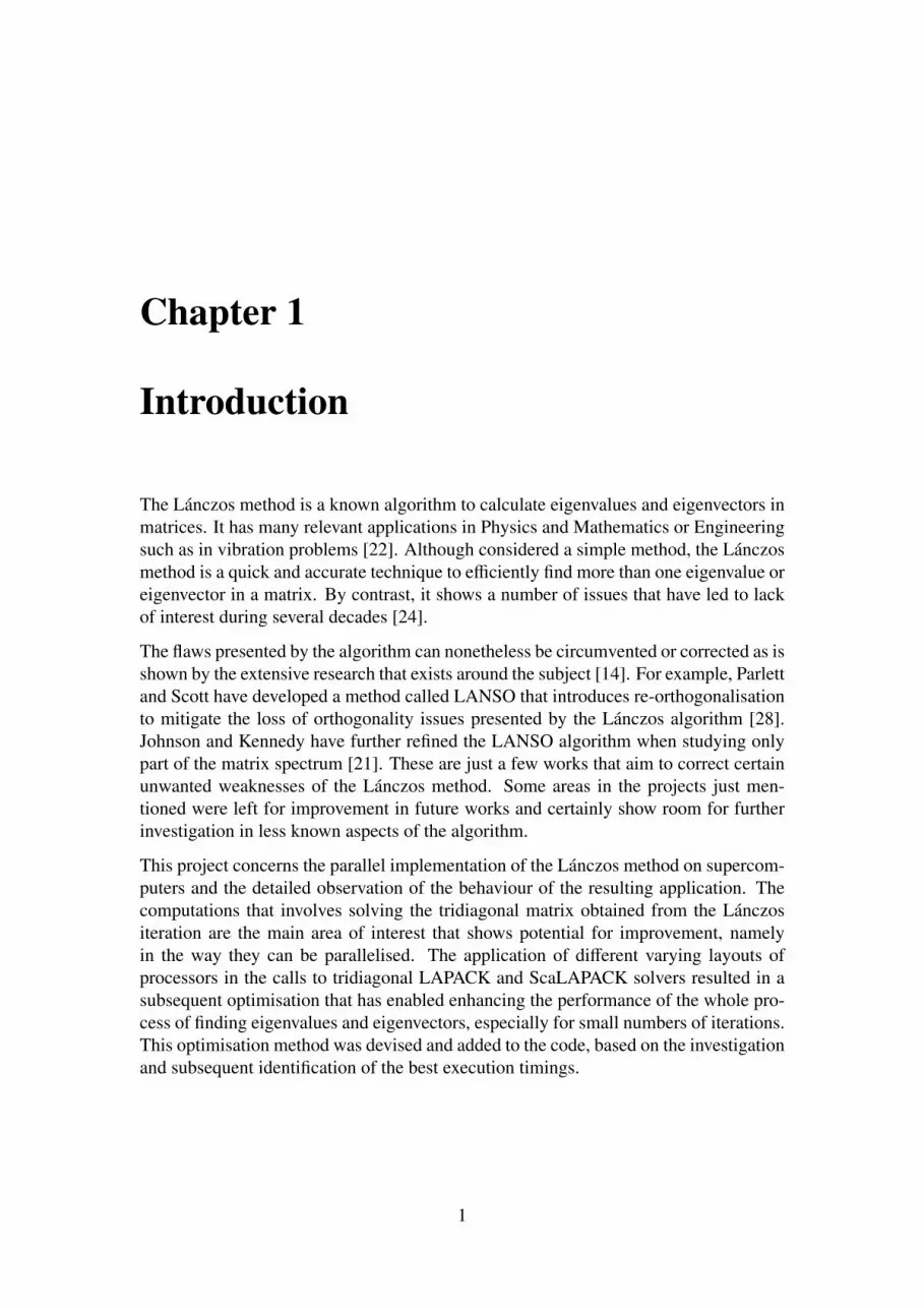
MPI communicators are predetermined groups of processes together with a communi-cation context. They define a communication domain [32], that is, a working space inwhich processes can communicate with each other independently of the outside envi-ronment. This is an essential concept of MPI since any MPI operation runs within acommunicator and therefore within a group of processes. The default or universal com-municator is called MPI_COMM_WORLD and consists of all the processes allocatedto an MPI application. This mechanism allows different MPI tasks to be performed inparallel on specific groups of processes independently isolated from others. This is ofparticular interest, for example, in hierarchical algorithms or problems that can be di-vided into subtasks, especially if taking into account the limited size of cache memories[34].

MPI_Comm_split() is an MPI C function that divides a communicator into smaller sub-communicators. Each process in a communicator gets a specific rank number rangingfrom 0 to size − 1 with size being the number of processors in the communicator. Eachsub-group issued from MPI_Comm_split contains processes with the same colour anda new rank number valid within the sub-communicator is defined by the key parameter.This features will allow creating subgroups of processes within which a ScaLAPACKoperation can be carried out, as stated further in the text.

9

MPI_Comm_world

subcomm�1 subcomm�2

colour�=�2colour�=�1

1 2

34

5

6

87

12

3

4

5

6

7 8

109

Figure 2.1: MPI communicators sub-division using MPI_Comm_split

2.3 Numerical linear algebra libraries

2.3.1 LAPACK

The LAPACK software library is a set of Fortran 90 subroutines for solving LinearAlgebra problems, such as linear systems of equations, and eigenvalue problems. Ac-cording to the documentation, LAPACK can handle with no difficulties dense and bandmatrices but not sparse ones. Its efficiency lies in the fact that during computation,memory accesses take advantage of the cache hierarchy of the machine; in the case ofmatrix operations using blocked access to data, for example. LAPACK works in a se-quential fashion as it was designed for a single thread of execution. Being serial and ifran on a distributed memory architecture, each core processes the same problem with-out any parallelisation and distribution of computation and data. LAPACK thereforeimposes a limitation on the size of the problems that can be tackled, which is dependenton the amount of the memory available on each core.

2.3.2 ScaLAPACK

LAPACK and ScaLAPACK are dependent of two other underlying libraries, namelyBLAS (Basic Linear Algebra Subprograms) for computation and BLACS (Basic Lin-ear Algebra Communication Subprograms) for communication[5][11]. ScaLAPACKwas written in Fortran 77 following a SPMD model (Single Program Multiple Data)with the exception of a few subroutines that were coded in C to comply with IEEEarithmetic. ScaLAPACK is the parallel version of LAPACK; it is a library of highlyoptimised and highly performing subroutines for solving linear algebra problems. Ituses MPI in communications between cores when sharing data or information and isparticularly well suited for MIMD architectures that implement the distributed memorymessage passing paradigm. For example, according to the documentation, the ScaLA-PACK library achieves high efficiency on Cray T3 series and IBM SP series.

10

scaLAPACK

PBLAS

LAPACK BLACS

BLAS Message Passing Primitives(MPI/PVM etc.)

Global

Local

Figure 2.2: ScaLAPACK Software Hierarchy[5]

The ScaLAPACK model is hence a layered model and ScaLAPACK sits on top of sev-eral existing libraries (see Fig. 2.2). The whole forms a stack of layered functionalityin which each level interacts with the others. The basis of ScaLAPACK is the PBLAS(Parallel BLAS) that implements distributed memory versions of the BLAS linear al-gebra subroutines (level 1 through level 3). Inter-processes communications are thusensured internally through calls to BLACS subroutines. As it can be seen in Fig. 2.2,the components below the dashed line operate at a level local to each processor andthose above at a global level across all processors: the process of distributing matri-ces and vectors across a number of cores belongs to the global level and will use itsassociated subroutines.

ScaLAPACK was designed for and is well suited for dense and band matrices but oneof its limitations resides in its poor handling of sparse matrices, which were used inthis project. ScaLAPACK distributes the matrices over a range of processors and thussolves memory limitations at the node level when handling large matrices sizes.

2.3.3 BLAS, PBLAS, BLACS

The BLAS (Basic Linear Algebra Subprograms) is the mechanism that implements sub-routines to actually solve linear algebra problems, such as matrix-matrix multiplication,linear systems of equations, etc. The optimised design of BLAS subroutines can com-pensate for cache or TLB misses and allow performance to reach near peak values ifusing the optimal parameters specific to an architecture [5].

The PBLAS (Parallel Basic Linear Algebra Subprograms) was also designed for dis-tributed memory architectures and manages the parallelisation of sequential codes that

11

make use of BLAS operations such as matrix-matrix, matrix-vector multiplications,among others [7].

The BLACS (Basic Linear Algebra Communication Subprogram) corresponds to thecommunication layer of the ScaLAPACK model. It provides an interface that simplifiesmessage-passing on distributed-memory parallel machines including heterogeneous ar-chitectures [11].

2.3.4 BLACS context

As described above, in order to parallelise its operation, ScaLAPACK calls the BLACSlibrary. To implement ScaLAPACK calls in parallel, a logical grid of processes called aBLACS context must be defined. This grid establishes how MPI processes will exchangedata in parallel ScaLAPACK operations. A BLACS context is similar to an MPI sub-communicator (see Subsection 2.2.1) and once defined, each context will similarly runa single instance of ScaLAPACK. In other words, calls to ScaLAPACK subroutines areparallelised among all the processes existing in a context. In this dissertation, BLACScontexts were used with varying numbers of processes to assess the performance of thetridiagonal solvers.

As an example, different tasks can be assigned to different contexts depending on thedesired calculations. A grid of 1×3 processes (one dimensional) can be used to performa matrix-matrix multiplication while another context (e.g. 4 × 4 two dimensional) canbe used for an operation involving nearest-neighbour computation thus separating tasksand processes.

The BLACS can be used in conjunction with MPI such that a program coded in Cof Fortran can include MPI instructions and call to the BLACS library; furthermore,a mapping has to be done between an MPI sub-communicator and a BLACS contextduring the BLACS setup. The group of processes initially defined in the MPI sub-communicator will be the same as those used in the BLACS context. Once the setup ofMPI sub-communicators and BLACS contexts is complete, MPI code can execute callsto ScaLAPACK.

12

Chapter 3

Methodology

This chapter explains in detail the techniques and methods that were employed in im-plementing the concepts previously exposed in Chapter 2. These notions were trans-lated into C code which was destined to run in parallel on a supercomputer with morethan 76,000 cores. The chapter starts with a description of the computational resourcesthat were made available and then carries on with the procedure utilised to achieve thecurrent project. Then follows a precise outline of the implementations of the severalalgorithms presented in Subsections 2.1.4, 2.1.5 and 2.1.6 as well as of the tridiagonalsolvers. The chapter ends up by refering to the smaller investigation conducted aboutthe placement of MPI processes on computational nodes and their core affinity.

3.1 Hardware architectures

3.1.1 Morar

Morar is a machine accessible to postgraduate students at the School of Physics andAstronomy of the University of Edinburgh. It consists of a Dell PowerEdge C6145equipped with 4xAMD Opteron(TM) Processor 6276 totalling 64 cores with per node.It is made of two computational nodes, each one basically a 64-core shared-memorysystem, with 4 AMD Bulldozer 16-core processors (2.3 GHZ, 16 C, 16 M L2). The 4processors share 128 GB (16 x 8 GB dual rank) of memory on each node accessed in aUMA (Uniform Accessed Memory) fashion.

This machine was used for the development of all the steps in building the application,because the process of coding, compiling and running the program on Morar is ratherquicker than on ARCHER (see Subsection 3.1.2). Nonetheless, it proved to be some-times limited by the hardware. Once the code implemented and working, it was portedto ARCHER which was mainly used to scale up the implementations to much largerproblem sizes and to much higher number of cores.

13

3.1.2 ARCHER

ARCHER is part of the UK National Supercomputing Service and is at the base a CRAYXC30 machine with 3008 nodes which totals more than 72,000 cores [1]. The com-putational nodes are divided into several categories, namely: compute, services, joblauncher and login nodes.

Each compute node is made of two Intel Xeon E5-2697 processors (2.7 GHz, 12-corev2 - Ivy Bridge) with 64 GB of memory shared between them. These two processorsare connected between themselves by two Quick Path Interconnect (QPI). Each nodehas been designed with a NUMA (Non-Uniform Memory Access) layout, that is, eachgroup of 12 cores forms a NUMA region and can access 32 GB of memory. Addition-ally, there is another sub-category of compute nodes that makes further use of higherspeed memory, sharing 128 GB of memory. All compute nodes of both categories to-tal a number of 3008 nodes or 72,192 cores. By contrast, a login node on ARCHERcontains only one Intel Xeon E5-2697 processor and their main function is to provide anumber of services such as running the PBS job launcher.

All compute nodes are connected to each others through the Cray Aries Interconnectin a Dragonfly topology. That is, 4 compute nodes are connected to an Aries router,188 nodes form a cabinet and two cabinets make a group. Groups use optical connec-tions between them and can achieve a peak bisection bandwidth of 7200 GB/s, an MPIlatency of approximately 1.3 µs and an extra 100 ns over the optical links.

3.1.3 NUMA

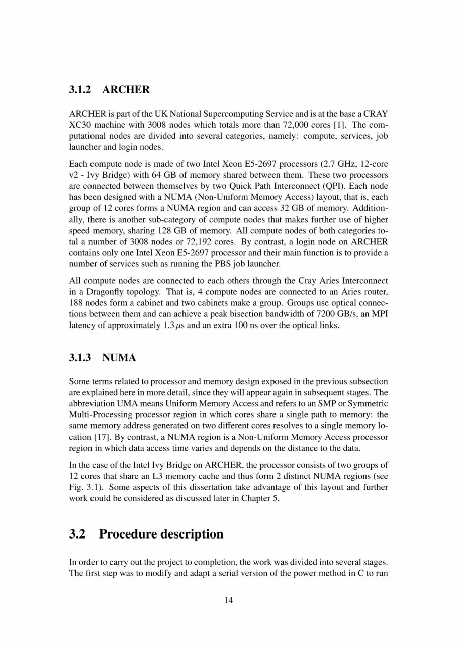
Some terms related to processor and memory design exposed in the previous subsectionare explained here in more detail, since they will appear again in subsequent stages. Theabbreviation UMA means Uniform Memory Access and refers to an SMP or SymmetricMulti-Processing processor region in which cores share a single path to memory: thesame memory address generated on two different cores resolves to a single memory lo-cation [17]. By contrast, a NUMA region is a Non-Uniform Memory Access processorregion in which data access time varies and depends on the distance to the data.

In the case of the Intel Ivy Bridge on ARCHER, the processor consists of two groups of12 cores that share an L3 memory cache and thus form 2 distinct NUMA regions (seeFig. 3.1). Some aspects of this dissertation take advantage of this layout and furtherwork could be considered as discussed later in Chapter 5.

3.2 Procedure description

In order to carry out the project to completion, the work was divided into several stages.The first step was to modify and adapt a serial version of the power method in C to run

14

Figure 3.1: Cray XC30 Intel Xeon compute node architecture [19].

in parallel on multicore architectures. Therefore, the initial code was parallelised to runon several cores, first developed on Morar (see Subsection 3.1.1) it was then ported toARCHER (details in Subsection 3.1.2). Once a fully working version was implemented,the power method code was transformed into a Lánczos method, first serially then inparallel. Again, the first versions were developed on Morar then ported to ARCHERto run with bigger matrices and with large numbers of processes. The following stepinvolved adding a tridiagonal solver to calculate the eigenvalues of the matrix createdby the Lánczos algorithm at each iteration. The tridiagonal solver was implementedby means of a call to the LAPACK software library. It should be noted that calls tothe LAPACK are effected independently on each core, in a serial fashion without anycommunication between processes.

The next stage consisted of replacing the call to the serial LAPACK solver by a callto a parallel tridiagonal solver in the ScaLAPACK library. ScaLAPACK is the parallelversion of LAPACK in which computation is distributed among processors. After theimplementation of the solvers, the resulting behavior of the code was investigated. Theobjective of the investigation was to examine the performance of the tridiagonal solverwhile allocating different subsets of MPI processes to ScaLAPACK. During the tests,the code was run with a total of 384 cores but smaller numbers of processes were allo-cated in turns to the solvers. These smaller groups of processes are therefore utilised toexecute a single instance of ScaLAPACK in parallel.

The subgroups were created with different numbers of cores as illustrated in Table 3.1and employed to create MPI sub-communicators and BLACS contexts, which werethen used by the respective tridiagonal solver when executing. For example, with atotal of 384 cores allocated to the program, the code was tested first with 192 groups of

15

2 processors, then as second test was carried out with 96 groups of 4 processors, etc.

This investigation was mainly achieved on ARCHER, the larger supercomputer, butMorar was still used in some initial tests with small numbers of processes. The timetaken by the solvers running with different numbers of cores was subsequently recorded.Based on the timings obtained, the code was then optimised. This optimisation wasachieved by inserting switching points at which the best processor layouts were swappedin, resulting in the code being executed with the best performing configurations, at alltimes.

A smaller investigation of the placement of the MPI processes on cores during the cre-ation of the sub-communicators was carried out at the same time. This verificationincluded the insertion of code that access lower level aspects of the functioning of pro-cessors. It was verified that the processes grouped in sub-communicators were beingmapped to the harware nodes respecting the layout of the processor cores, that is, re-specting the NUMA regions of the processors (more details in Sections 3.10 and 4.6).The core affinity of the MPI processes was also checked.

The last stage of the project consisted of implementing in the code a second call toScaLAPACK to solve the eigenvectors of the matrix. However, due to poor existingdocumentation this stage but was left for future work.

Number ofprocesses per group

Total numberof groups

Total number ofScalapack instances

384 1 1192 2 296 4 448 8 824 16 1612 32 328 48 486 64 644 96 962 192 192

Table 3.1: Number of processes per MPI sub-communicator with the resulting numbersof subgroups and of ScaLAPACK instances.

The next sections of this chapter will carry on exposing the complete details of theprocedure just outlined.

3.3 Implementation of a parallel power method

The current project was initiated with a given serial implementation of the power methodthat was then modified to run in parallel. This section will outline the main operations

16

involved in the implementation of the algorithm.

Given an initial serial piece of code, this was then adapted to run on distributed-memoryparallel computers such as Morar and Archer. During the parallelisation of the powermethod, two different versions have been coded: a first one in which the data involved inthe calculations were replicated across all the processors and a second version in whichdata were distributed over the processors. Here data means the vectors necessary tocomputations since the matrix was initially distributed. In the first (replicated) version,the entire vectors were made available on all the processors, (see Algorithm 3) whereasin the second (distributed), just a section of each vector was stored on each core (seeAlgorithm 4).

The main computation of the power method comprises the matrix-vector multiplicationv(k) B Av(k−1) (see Algorithm 1) and it is the most important operation of the algorithmsince it represents the biggest percentage of the time taken by the whole iteration. Italso offers great potential to be exploited in parallel when scaling up to higher numbersof processors.

When scaling up to high numbers of cores, matters such load balance, synchronisationand communication costs must be taken into consideration during the design of theparallel program. As a quick reference, load balance refers to the way data ought tobe partitioned and distributed to the working elements: in the end, all processors mustideally have the same amount of work to process, such that none is left idle while othersare computing. Synchronisation of data must also be ensured since some operations ofthe power method like normalisation need the computational results of all the processorsto proceed. Communication overhead is the third and last issue to keep in mind whenit comes to sharing data across many working elements. Communications can largelyinfluence and penalise the performance of the algorithm, especially when running overlarge numbers of elements [14].

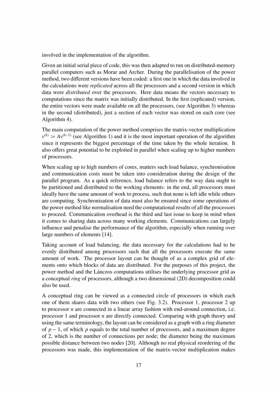
Taking account of load balancing, the data necessary for the calculations had to beevenly distributed among processors such that all the processors execute the sameamount of work. The processor layout can be thought of as a complex grid of ele-ments onto which blocks of data are distributed. For the purposes of this project, thepower method and the Lánczos computations utilises the underlying processor grid asa conceptual ring of processors, although a two dimensional (2D) decomposition couldalso be used.

A conceptual ring can be viewed as a connected circle of processors in which eachone of them shares data with two others (see Fig. 3.2). Processor 1, processor 2 upto processor n are connected in a linear array fashion with end-around connection, i.e.processor 1 and processor n are directly connected. Comparing with graph theory andusing the same terminology, the layout can be considered as a graph with a ring diameterof p − 1, of which p equals to the total number of processors, and a maximum degreeof 2, which is the number of connections per node; the diameter being the maximumpossible distance between two nodes [20]. Although no real physical reordering of theprocessors was made, this implementation of the matrix-vector multiplication makes

17

P1

P4

P2

P3

Figure 3.2: Ring layout of 4 processors

use of the processors as if they were disposed in such way.

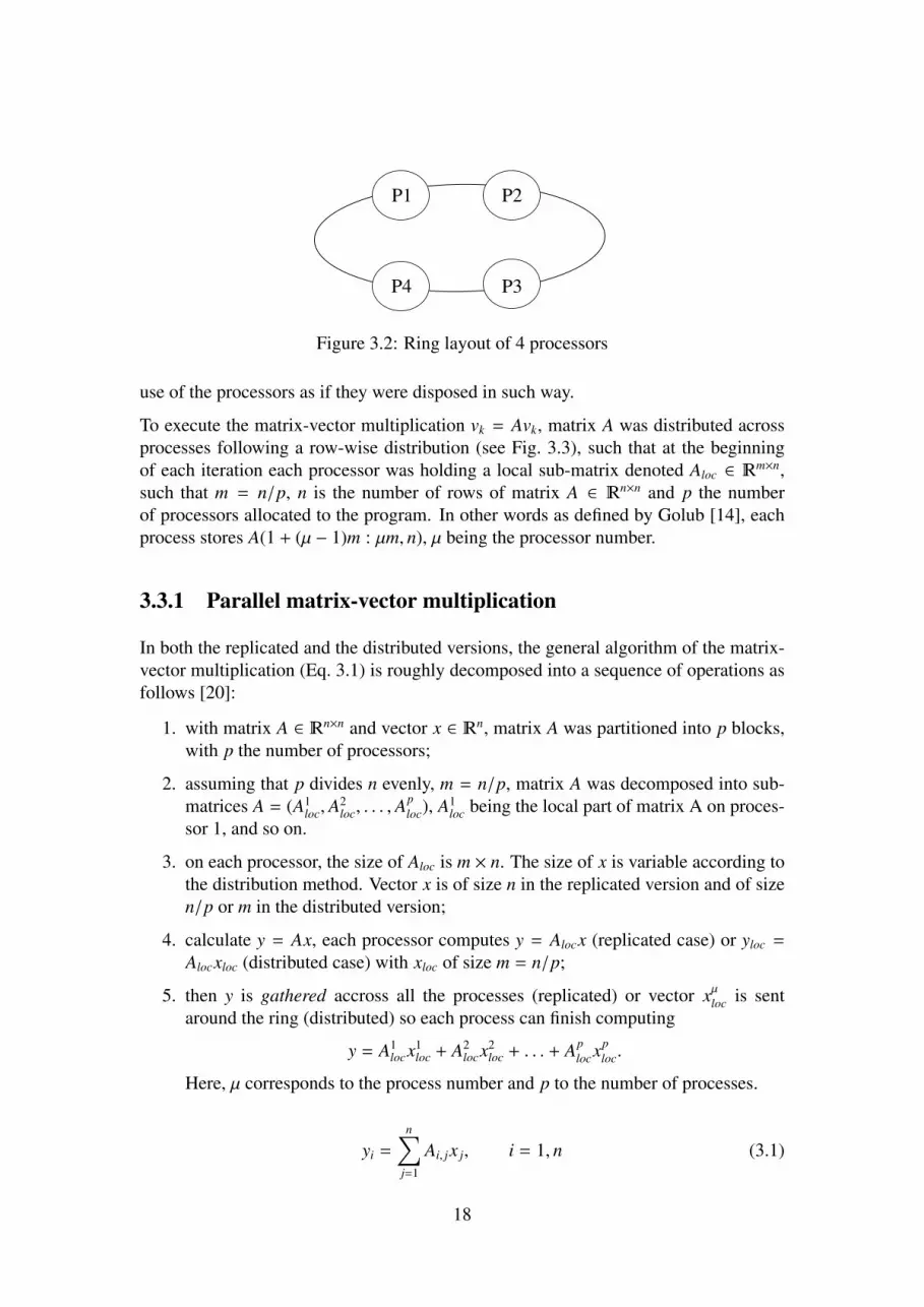
To execute the matrix-vector multiplication vk = Avk, matrix A was distributed acrossprocesses following a row-wise distribution (see Fig. 3.3), such that at the beginningof each iteration each processor was holding a local sub-matrix denoted Aloc ∈ �

m×n,such that m = n/p, n is the number of rows of matrix A ∈ �n×n and p the numberof processors allocated to the program. In other words as defined by Golub [14], eachprocess stores A(1 + (µ − 1)m : µm, n), µ being the processor number.

3.3.1 Parallel matrix-vector multiplication

In both the replicated and the distributed versions, the general algorithm of the matrix-vector multiplication (Eq. 3.1) is roughly decomposed into a sequence of operations asfollows [20]:

1. with matrix A ∈ �n×n and vector x ∈ �n, matrix A was partitioned into p blocks,with p the number of processors;

2. assuming that p divides n evenly, m = n/p, matrix A was decomposed into sub-matrices A = (A1

loc, A2loc, . . . , A

ploc), A1

loc being the local part of matrix A on proces-sor 1, and so on.

3. on each processor, the size of Aloc is m × n. The size of x is variable according tothe distribution method. Vector x is of size n in the replicated version and of sizen/p or m in the distributed version;

4. calculate y = Ax, each processor computes y = Alocx (replicated case) or yloc =

Alocxloc (distributed case) with xloc of size m = n/p;

5. then y is gathered accross all the processes (replicated) or vector xµloc is sentaround the ring (distributed) so each process can finish computing

y = A1locx1

loc + A2locx2

loc + . . . + Aplocxp

loc.

Here, µ corresponds to the process number and p to the number of processes.

yi =

n∑j=1

Ai, jx j, i = 1, n (3.1)

18

P1 

P2

P3

P4

Figure 3.3: Row-wise matrix partition over 4 processors.

3.3.2 Parallel replicated

Based on the knowledge previously exposed, two versions of the parallel power methodwere then developed.

In the first, the replicated parallel version (see Algorithm 3), each processor holds acopy of the whole initial vector v(0) obtained randomly and normalised as explainedin Subsection 2.1.3. In the next step, the matrix-vector multiplication zloc = Avk−1

is performed with the local portion of matrix A. The result is a partial vector thatis gathered in the following step across all the processors by means of an all-gatheroperation.

An all-gather operation (also known as all-to-all broadcast) is a collective commu-nication process that is effected by all processors involved in the calculation: eachprocessor receives the local results of all the other processors involved in the com-putation. The portions received are then concatenated and stored in a vector of sizen. This is implemented in MPI by the functions (or subroutines) MPI_Allgather andMPI_Allgatherv: both MPI functions are collective functions, however MPI_Allgathervdiffers from MPI_Allgather in that it offer greater flexibility by allowing different pro-cesses to transmit different data sizes, therefore MPI_Allgatherv is called the vectorvariant of MPI_Allgather. The MPI_Allgather operation performs O(n2) communica-tion operations for n processors.

The vector resulting from the received parts of all the processors is then normalisedand used in the following matrix-vector multiplication in step 6 of Algorithm 3. Again,the partial portion obtained on each process is gathered in a vector across all processesthrough another collective call. The eigenvalue λ is then calculated with a dot productbetween vectors v(k) and w(k) in step 8. The last step computes the subtraction w(k)−λv(k)

in order to assess the stopping condition: i.e. the algorithm will stop when the condition||Ay − λy|| is below the given tolerance, in the present case machine ε.

19

Algorithm 3 Parallel Power Method (Replicated)Require: given matrix Aloc ∈ �

mloc×n and vectors v, z,w ∈ �n and vtmp,wloc, zloc ∈ �mloc

with mloc = m/p, m the number of rows of matrix A ∈ �m×n and p the number ofprocessors allocated to the program.

Require: λ is a scalar.Require: choose random vector v(0) such that ||v(0)||2 = 1Ensure: λ is the scalar holding the dominant eigenvalue.

1: while ||Alocv(k) − λv(k)tmp||2 >= ε do

2: z(k)loc B Alocv(k−1)

3: allgather(z(k)loc, z

(k))4: v(k) B z(k)/||z(k)||2

5: w(k)loc B Alocv(k)

6: allgather(w(k)loc,w

(k))7: λ B v(k) · w(k)

8: v(k−1) B v(k)

9: w(k) B w(k) − λlocv(k)

10: end while

3.3.3 Parallel distributed

A second version of the parallel power method was implemented when the replicatedone was working correctly. In this new implementation, a number of vectors employedin the several operations of the algorithm were distributed accross processes (see Algo-rithm 4). Each processor holds portions of vectors instead of entire vectors and performsits calculations with its local data. The matrix is still stored in row-wise fashion on eachprocess.

To recapitulate, in order to perform the matrix-vector multiplication vk = Avk, matrixA was distributed across processes following a row-wise distribution (see Fig 3.3) andvector vk following the store-by-row method from Golub (as explained in the diagrambelow) [14]. This resulted in each process holding a local sub-matrix denoted hereAloc ∈ �

m×n and a partial vector vloc ∈ �m.

As an example, assuming that n = m× p, with n = 16, the size of the vector v and p = 4and using the store-by-colum method [14] then the resulting vector decomposition canbe defined as:

v =P1 P2 P3 P4

v1, v2, v3, v4 v5, v6, v7, v8 v9, v10, v11, v12 v13, v14, v15, v16

After the distribution, each process has been assigned the partial vector vloc(1+(µ−1)m :µm) ∈ proc(µ).

The general basic algorithm [14] [20] for the whole sequence of operations summarisesas follows: initially proc(µ), with µ the process number, stores vµ and µth block row ofA, then each process computes

20

yµ =

p∑τ=1

Aµτvτ (3.2)

where (Aµτ, vµ) is local data and (vτ, τ , µ) non-local. To complete its calculationproc(µ) needs vτ data from its neighbour. To this effect, the partial non-local vector vτis transmitted through the conceptual ring; when the sub-vector is received by processµ operation is resumed and calculations completed. Waiting for data is implementedthrough underlying MPI mechanisms of sending/receiving data between processes, suchas non-blocking operations MPI_Issend, MPI_Irecv and MPI_Wait. Data circulates in amerry-go-round or ring-like fashion across processes, upon completion process µ holdsy(1 + (µ − 1)m : µm).

Send and receive are message-passing operations that send vector v to the left or receiveit from the right neighbour of the processor being considered. In the present case, eachworking element performs a number of partial calculations with the local data allocatedto it and then sends vector v to its neighbour when completed. This same workingelement receives data from its second neighbour, theoretically at the same time, that isignoring communications overheads.

iteration Proc(1) Proc(2) Proc(3) Proc(4)1 y1 B A11x1 y2 B A21x1 y3 B A21x1 y4 B A41x1

2 y1 B A12x2 y2 B A22x2 y3 B A32x2 y4 B A42x2

3 y1 B A13x3 y2 B A23x3 y3 B A33x3 y4 B A43x3

4 y1 B A14x4 y2 B A24x4 y3 B A34x4 y4 B A44x4

Table 3.2: Vectors being swapped around processors

Figure 3.4 and Table 3.2 give an overview of the inner functioning of the distributedmatrix-multiplication with 4 processes as an example. At iteration 1, process 1 willcompute y1 = A11x1, process 2 will compute y1 = A21x1, process 3 y1 = A21x1 andprocess 4 y1 = A41x1. The table then shows what data each processor holds and whichcomputation is being processed.

With the previous information in mind, algorithm 4 describes how the distributed par-allel power method was implemented in C code for the current dissertation. The mainsummarised steps comprise: the algorithm starts with an initial random vector createdlocally on each processor with size as described above; the vector is next normalised.In step 2, the local matrix-vector is carried out. In steps 3 to 9, the vector v(k−1)

loc iscirculated across processors, and the remaining matrix-vector multiplications are per-formed, according to the matrix-vector decomposition, including the data from all theother processors. The sum of all the results is accumulated in step 7. Steps 3 to 9 arerepeated until the whole matrix-vector multiplication is completed. The resulting vectoris then normalised in step 10. The local value of λ is calculated in step 13. Anotherdata exchange is effected between steps 14 and 21, this time involving vector vk, whichis necessary for the calculation of the matrix-multiplication of step 17 and of lambda in

21

Algorithm 4 Parallel Power Method (Distributed)Require: given matrix Aloc ∈ �

m×n and vectors vloc, zloc, vrecv, vtmp,wloc,wtmp ∈ �m with

m = n/p, n the number of rows of matrix A ∈ �n×n and p the number of processorsallocated to the program.

Require: norm, λloc and λglob are scalars.Require: right and le f t are respectively the right and left neighbours of the process

being considered.Require: choose random vector v(0)

loc such as ||v(0)loc|| = 1

Require: ε is the convergence threshold and is equal to machine epsilon.Ensure: λglob is the scalar holding the dominant eigenvalue.

1: for k B 1 to p do2: z(k)

loc B Alocv(k−1)loc

3: for i B 1 to number of processors - 1 do4: send(right, v(k−1)

loc )5: receive(le f t, v(k)

recv)6: z(k)

tmp B Alocv(k)recv

7: z(k)loc B z(k)

loc + z(k)tmp

8: v(k−1)loc B v(k)

recv

9: end for10: v(k)

loc B z(k)loc/||z

(k)loc||

11: v(k)tmp B v(k)

loc

12: w(k)loc B Alocv

(k)loc

13: λ(k)loc B λ(k)

loc + v(k)loc · w

(k)loc

14: for i B 1 to number of processors - 1 do15: send(right, v(k)

loc)16: receive(le f t, v(k)

recv)17: w(k)

tmp B Alocv(k)recv

18: λloc B λloc + v(k)recv · w

(k)tmp

19: w(k)loc B w(k)

tmp

20: v(k)loc B v(k)

recv

21: end for22: allreduce(λ(k)

loc, λ(k)glob)

23: v(k)loc B v(k)

tmp

24: w(k)loc B w(k)

loc − λv(k)tmp

25: norm B ||w(k)loc||

26: if norm < ε then27: exit28: end if29: end for

22

P1 {P2 {P3 {P4 {

iteration

1 2 3 4

Figure 3.4: Matrix-vector multiplication over 4 processors

step 18. Then in step 22, an allreduce operation is carried out that gathers all the localvalues of lambda of all the processes and summed them up. The obtained accumulatedvalue corresponds to the approximation of the dominant eigenvalue of matrix A. Fi-nally, in step 26, the norm of the residual is compared to a threshold, in this case againstmachine epsilon, if the value of ||Alocvk(k)

loc − λvk(k)tmp|| is less than ε then the algorithm can

be considered to have converged.

3.3.4 Conclusion

When dealing with huge matrices, for instance, in the order of millions of elements,the choice between the replicated and the distributed power method will significantlyimpact the overall performance of the algorithm. The size of the problem that can becomputed is limited by the amount of memory available on each core. The size of thematrices is less problematic since the matrices considered in this project are sparse;there are storage mechanims to efficiently store them such that less memory space isutilised per core. However, regarding the sizes of the vectors, in the replicated case,the entire vectors are stored on each core. Thus, it can be said that the replicated ver-sion of the code implies higher memory space requirements per core when comparedto the distributed option (see Algorithm 4). As a conclusion to this small observation,distributing vectors appears as a very sensible solution to overcoming the memory lim-itations of processors.

3.4 Serial Lánczos

The following stage of the project involved implementing a Lánczos method that com-puted the eigenvalues and the eigenvectors of a matrix A. This stage comprised trans-forming the previous implementation of the power method into a working parallel Lánc-zos algorithm.

To start with the task, a serial version of the Lánczos method was implemented in C,

23

based on Golub’s algorithm [14]. The code was written by modifying the distributedpower method code and turning it into a valid Lánczos algorithm. At least three differentversions were coded, during initial tests, based on different versions of the algorithmfrom Golub [14], Parlett [27] and Paige [24][25]. For the purpose of this dissertation,Paige’s version was the one retained, as it was the simplest, with few data structuresand proven to be effective [8]. The algorithms all achieve the same purpose with slightdifferences in the order of instructions or the number of vectors used but most of allPaige’s algorithm is the most numerically stable [28] [25]. Paige’s version is describedin Algorithm 2.

3.5 Parallel Lánczos

After implementing the serial Lánczos method, and subsequent verification of the cor-rectness of the results, the code was modified to run on several processors. In orderto parallelise the main operation of the algorithm, the matrix-vector multiplication, thesame technique as for the power method was used.

As a result, a parallel algorithm was thus developed and can be described as follows.Going through each step of Algorithm 5, as stated in previous algorithms, a vector r1

with norm 1 is initially created then used in the matrix-vector multiplication of step2. The vector is local to each processor which means it has a size of n/nprocs withn the number of rows of matrix An×n and nprocs the total number of cores allocatedto the program. Between steps 3 and 9, the data is exchanged across processes. Thatis each process sends vector rk to its right neighbour and receives the correspondingvector from its left neighbour. Each process can then proceed to compute the remainingmatrix-vector multiplications. The code will loop through the several portions of matrixA as long as there are columns to process according to the previously explained matrixand vectors decomposition.

In step 10, the local value of α is calculated, and in step 11, each local value on eachprocess is summed up through an MPI all reduce operation. When the algorithm hasconverged the sequence of diagonal elements [α1, α2, . . . , αn] of the resulting tridiagonalmatrix T j is generated. Step 14, the value of the global α is added to the vector Alphafor subsequent use. In steps 13 and 14, the current number of iteration k is tested againstthe size n of matrix A and of vectors to check if no unnecessary iteration is carried out:no significant result is obtained if the algorithm performs more iterations than there arematrix or vectors elements.

At stage 16, the Lánczos vector qk is calculated by subtracting from its current value, thedot product between α and r, and the dot product between the previous βk−1 and rk−1.At this point, the q vectors (also called Lánczos vectors) can be stored in some way,to secondary storage or to RAM memory, if needed for possible future computations.They will have to be stored to memory is there are to be re-orthogonalised or if neededto construct the eigenvectors [28] [21]. The question of how to store the Lánczos vectors

24

q was left for future work since it requires proper investigation beyond the scope of thepresent project. In step 17, the vector rk is stored for the next iteration and in step 18,the local portion of the Lánczos vector q is normalised to obtain the value of the sub-diagonal element β of the tridiagonal matrix T j corresponding to the current iteration.At stage 19, the vector r necessary in the next iteration is computed by dividing thevector q by the scalar β. Finally, in step 20, the current value of β is stored for the nextiteration and into the vector of sub-diagonal elements of matrix T j.

Algorithm 5 Lánczos Parallel AlgorithmRequire: given matrix Aloc ∈ �

mloc×n and vectors qloc, rloc, qtmp, rtmp, Alpha and Beta ∈�mloc with mloc = m/p with m the number of rows of matrix A ∈ �m×n and p thenumber of processors allocated to the program.

Require: α and β are scalars.Require: right and le f t are respectively the right and left neighbours of the process

being considered.Require: initialise r1 B random vector with norm 1, r0 B 0, β1 B 0Ensure: α and β are the diagonal and the super-diagonal elements of Tk.Ensure: Alpha contains the diagonal elements of the newly created matrix T j and Beta

the sub-diagonal ones.1: for k = 1, 2, · · · , n − 1 do2: qk

loc B Alocrkloc

3: for i = 1, 2, · · · , numprocs − 1 do4: send(right, rk

loc)5: receive(le f t, rk

tmp)6: qk

tmp B Alocrktmp

7: qkloc B qk

loc + qktmp

8: rkloc B rk

tmp9: end for

10: αkloc B qk

loc · rkloc

11: allreduce(αkloc, α

kglob)

12: Alphak B αkglob

13: if k = n then14: STOP15: end if16: qk

loc B qkloc − α

kglobrk

loc − βk−1rk−1

loc

17: rk−1loc B rk

loc18: βk B

∥∥∥qkloc

∥∥∥19: rk

loc B qkloc/β

k

20: Betak B βk−1 B βk

21: end for

25

3.6 Parallel L2-normalisation

The L2-norm is a normalisation calculation present in all the algorithms presented be-forehand, such as at line 18 of the parallel Lánczos algorithm (Algorithm 5), or line 10of the distributed parallel power method (Algorithm 4). The serial algorithm (refer toSubsection 2.1.3) had to be adapted to perform its computation in parallel.

Algorithm 6 Parallel L2-normRequire: given vector vloc ∈ � of size m = n/p with n the number of rows of matrix

A ∈ �n×n and p the number of processors allocated to the program1: normloc B vloc · vloc

2: allreduce(normloc, norm)3: norm B

√norm

The parallel L2-norm is made of 2 steps: first, all the elements of the vector involved aresquared and then summed up. Second, the square root of the previous sum is obtained.

Algorithm 6 is explained as follow: in line 1, each MPI process calculates a vectordot product between the local vector vloc and itself. In line 2, since the whole vectoris needed for the normalisation, an all reduce operation is carried out across all theprocesses involved in the computation. An all reduce is an MPI global communicationthat gathers all values of normloc by means of a sum that is accumulated in norm. Inline 3, the square root of the result of the previous line is calculated, which yields theL2-norm of vector v.

3.7 Tridiagonal solvers

The final step of the process of finding eigenvalues and eigenvectors consists in solvingthe tridiagonal matrix T produced at each iteration by the Lánczos method. Two soft-ware packages are available with tridiagonal solver subroutines that can perform thenecessary computations, namely the LAPACK and the ScaLAPACK. Both have similarsubroutines with the difference that the LAPACK processes the tridiagonal solver seri-ally on each core and no true parallelism is exploited and the ScaLAPACK executes thetridiagonal solver in parallel, hence taking advantage of the underlying hardware.

Therefore two different options are possible:

− with LAPACK, the tridiagonal solver is called independently on each process andthe eigenpairs are computed serially. This solution however is limited by the localmemory size available on each node;

− with ScaLAPACK, the library is then responsible of internally taking care of allthe parallel aspects of solving the tridiagonal matrix, such that an optimal workbalance is achieved and true parallelism exploited.

26

3.7.1 Implementation of a LAPACK eigensolver with DSTEV

The LAPACK subroutine chosen to solve the tridiagonal matrix issued from each Lánc-zos iteration was DSTEV. The LAPACK DSTEV Fortran subroutine (and any other LA-PACK xDSTEVx subroutines) computes all the eigenvalues and optionally the eigen-vectors of a given real symmetric tridiagonal matrix by applying the QR method. TheQR iteration applies a series of similarity transformations to the tridiagonal matrix un-til its diagonal elements are transformed into the eigenvalues [10]. DSTEV actuallyemploys QR for small matrices (size <= 25) and switches to a different algorithm, di-vide and conquer, for matrices sizes greater than 25 [9]. The subroutine can be fasterthan others that use QR as well, for example xSTEQR, but needs more working space(O(2n2) or O(3n2)) [4].

One of the other reason that justifies the choice of DSTEV instead of any other is thatbesides offering the option of returning eigenvectors if wanted, DSTEV can also beeasily swapped by DSTEVZ that allows selecting a range of eigenvalues by defining itslower and an upper bound during the call [2] [21].

Since the LAPACK library was written in Fortran 77, a C wrapper was necessary tofunction as interface between the two languages. The C wrapper is a simple C func-tion that calls the Fortran subroutine. However, a number of preparations need to doneprior calling the Fortran DSTEV subroutine. Any Fortran subroutine apply the call-by-reference mechanism when taking arguments during the call, therefore the argumentshad to be given as pointers in C so Fortran can makes proper use of them (see List-ings 3.1 and 3.2).

1 i n t d s t e v ( char j obs , i n t n , double ∗d , double ∗e , double ∗z , i n t ldz ,double ∗work )

2 {3 i n t i n f o ;4 d s t e v _ (& jobs , &n , d , e , z , &ldz , work ) ;56 re turn i n f o ;7 }

Listing 3.1: C wrapper

1 SUBROUTINE DSTEV( JOBZ , N, D, E , Z , LDZ, WORK, INFO )2 ∗ . . S c a l a r Arguments . .3 CHARACTER JOBZ4 INTEGER INFO , LDZ, N5 ∗ . .6 ∗ . . Ar ray Arguments . .7 DOUBLE PRECISION D( ∗ ) , E ( ∗ ) , WORK( ∗ ) , Z ( LDZ, ∗ )

Listing 3.2: LAPACK DSTEV Fortran subroutine

The subroutine DSTEV takes a series of parameters as arguments that need to be de-termined before the call. For example, given the option ’N’ or ’V’, it outputs only theeigenvalues or both the eigenvalues and the eigenvectors. The diagonal and the sub-diagonal elements of the tridiagonal matrix are given in the form of arrays, respectively

27

D and E. The other arrays passed as argument are working space and the actual result-ing eigenvectors, if wanted. Upon completion, it returns info a flag indicating failureor success. If info is null, then the call was successful; if info is equal to a number -ithen the ith argument passed to the function was wrong; if info is positive, the compu-tation failed to converge and in this case the number returned in info corresponds to thenumber of off-diagonal elements that failed to converge to zero.

On Morar, the libraries had to be linked to the executable in order to compile. Thelocation of the library has to be known by the compiler, so the following flags wereincluded in the Makefile:

LFLAGS= -lm -lpgftnrtl -lrtLDFLAGS=-L/usr/lib64/scalapack/LIBS= -lgfortran -lscalapack -llapack -lblas

On the other hand, compilers and linkers on ARCHER do not need location flags atcompile time. By default, all users on ARCHER start with the Cray programmingenvironment loaded (PrgEnv-cray), the MPI (cray-mpich) and Cray LibSci (cray-libsci,including BLAS, LAPACK, ScaLAPACK) libraries included in their environment [1].

3.7.2 ScaLAPACK

The next stage of the present dissertation was to implement the tridiagonal solver inparallel using the ScaLAPACK library.

In order to implement a call to a ScaLAPACK subroutine, a predefined sequence ofoperations must be followed: first, a process grid must be initialised that will act ascommunication context in which ScaLAPACK executes; second, the matrix must bedistributed among the given MPI processes; third, the actual call to the subroutine iseffected; last, the process grid is released. Similarly to LAPACK, ScaLAPACK Fortransubroutines are accessed through C functions such as mentioned in Listings 3.1 and3.2).

3.7.3 Implementation of a ScaLAPACK eigensolver with PDSTEBZ

Recalling the serial implementation of the tridiagonal solver (see Subsection 3.7.1), thesubroutine DSTEV in LAPACK was the one chosen to find the eigenpairs of matrixT . Since there is no parallel version of DSTEV in ScaLAPACK, PDSTEBZ was thesubroutine chosen for the current project.

PDSTEBZ in ScaLAPACK is a parallel eigensolver that computes the eigenvalues of areal symmetric tridiagonal matrix A using the bisection algorithm. One of the featuresof this subroutine that dictated its choice was that a range of values can be specified dur-ing the call such that only the eigenvalues corresponding to this range are calculated.

28

The subroutine implements an eigensolver in parallel and according to the documenta-tion a static partitioning is effected at the beginning of the subroutine before the matrixis internally distributed [15]. For a matrix An×n with k corresponding eigenvalues, thebisection algorithm completes the computations in O(kn) operations [3].

Similarly to DSTEV, PDSTEBZ uses a sequence of arguments that must be definedbefore the actual call. Again, the diagonal and the sub-diagonal elements of the tridi-agonal matrix resulting from the Lánczos iteration are input as arguments in the call toPDSTEBZ. A BLACS context must also be defined and included so the subroutine willuse the grid of processors provided (refer to Subsection 2.3.4). On output, the eigenval-ues are contained in an array of size n, the order of the matrix. A number of other arraysare to be setup before the call that the subroutine uses as inner working space [2].

A simplified model of the program was built to simplify the implementation of thesolver and the verification of the results output. Instead of calculating the diagonaland sub-diagonal elements of the newly formed tridiagonal matrix T generated by theLánczos iteration, the simplified program was designed to load a predefined set of val-ues to simulate these results (namely vectors containing α’s and β’s of matrix T ). Thissimplification allowed an easier manipulation of the input parameters during the callto the subroutine resulting in a lighter program; this small program greatly helped theimplementation of ScaLAPACK routines which due to the lack of documentation is nota straightforward process.

At the start of the tests, PDSTEBZ was executed with a BLACS context of 24 cores, thedefault number of cores on each node on ARCHER. The BLACS context is a closed en-vironment of MPI processes that execute in parallel a single instance of a ScaLAPACKsubroutine. Therefore the solver was parallelised across a group of 24 processes. Asusual, the code was initially developed on Morar with small numbers of cores and thenported to ARCHER to run with bigger matrices sizes on higher numbers of processes.

It was decided that the user of the program could choose any arbitrary number of coresper sub-communicator. Hence, a number of instructions were inserted in the code toaccept a command line argument that defined at runtime the number of cores to runScaLAPACK. The program is executed inserting the argument after the name of theprogram in the submission script (both on Morar and on ARCHER), e.g.:

1 . / l a n c z o s <number o f p r o c e s s o r s p e r sub−communicator > .

If no argument is provided at the command line, the program uses the default number ofprocessors per context, which was defined as 24 (the default number of cores per nodeon ARCHER). Since the program was designed to be executed on ARCHER, by defaulteach computational node will run an instance of ScaLAPACK.

To further explain how the subroutine PDSTEBZ was implemented the next subsectiondescribes the way MPI sub-communicators were created.

29

scaLAPACKPDSTEBZ &

PDSTEIN

24 cores 12 cores

48 cores

Figure 3.5: ScaLAPACK subroutines executing over BLACS contexts with 12, 24 and48 processors

3.7.4 CBLACS implementation

In order to correctly make calls to the ScaLAPACK library, the code must follow acorrect sequence of instructions. The first step consists of initialising a grid layout orBLACS context. A BLACS context can be seen as a restricted group of processorsthat can communicate between themselves (intra-context communications) but with noconnection with the outside environment (inter-contexts communications). The BLACScontext is created through a series of calls to BLACS subroutines, which were originallycoded in Fortran, but are accessed from the present code through calls to CBLACSwrappers. CBLACS is the C interface aimed at C programmers.

A series of parameters must be initialised in order to define the intended layout of thegrid. The result is a logical grid of processes that ScaLAPACK uses for the parallelisa-tion of its subroutines. For example, a ScaLAPACK subroutine destined to perform alinear algebra matrix-vector multiplication will split the work load among the processesincluded in the context by distributing the matrix and the vectors among these.

In order to initialise a CBLACS context, an MPI communicator had to be created. Thenumber of processes in each communicator is 24, which was hard-coded in the programas the default number of cores per context. This is due to the fact that the currentprogram was aimed to run on ARCHER which currently has 24 cores per computationalnode. As an example, if the program is launched with 192 cores or 8 nodes, each node

30

will run a single instance of ScaLAPACK, that is using the default of 24 cores percontext. If the user does not want to run the default number of cores per context, theprogram offers the option of inputting a command line argument at run time.

The command line argument should be provided when the program is launched with thejob submission script (.sge files on Morar and .pbs on ARCHER, see documentation onsubmitting jobs [1]). For example, when running the program with a command suchas aprun -n 192 ./lanczos 48, 192 cores will be allocated to the whole program andthis number will be divided into 4 groups of 48 processes that will run 4 instances ofScaLAPACK (for more details refer to Section 3.2).

A one dimensional layout of processes was used to build the BLACS grid, simply be-cause the diagonal and sub-diagonal elements of the tridiagonal matrix T j are stored intwo one-dimensional arrays.

The communicator is returned on output of the MPI subroutine MPI_Comm_split thattakes as arguments respectively the communicator that will be split and the resultingsub-communicator (see Listing 3.4). The other two arguments were defined as men-tioned in Subsection 2.2.1. On output of the splitting procedure, each process wasassigned a new rank number and encapsulated in a new communicator.

The CBLACS function Cblacs_gridinit() is the first to be called during the initiali-sation of the layout grid and takes a BLACS context as argument, in the form of aninteger. Since an MPI communicator cannot be directly mapped to a BLACS con-text or an integer, this mapping must undergo a translation process during initialisa-tion [35]. This issue is due to incompatibilities between the two different languages inboth libraries, namely Fortran 77 in ScaLAPACK and LAPACK, and C in CBLACS.Therefore, an intermediary step had to be inserted between the conversion of commu-nicators to contexts, through the use of C wrapper functions. A number of C func-tions were made available by the libraries designers to assist this process, such asCsys2blacs_handle(MPI_Comm SysCtxt) which maps an MPI communicator to an in-teger BLACS context handle. Hence, the several BLACS contexts were initialised asexplained as following:

1 i n t init_BLACS (MPI_Comm ∗ sub_communica tor , i n t ∗ r anks , i n t ∗ numprocs )2 {3 i n t BLACS_handle , BLACS_context ;4 . . .5 / / c r e a t e an i n t e g e r h an d l e from t h e MPI communicator6 BLACS_handle = C s y s 2 b l a c s _ h a n d l e (∗ sub_communica tor ) ;7 BLACS_context = BLACS_handle ;89 / / I n i t i a l i s e p a r a m e t e r s

10 n r o w s _ p r o c _ g r i d = 1 ; / / number o f rows i n t h e p r o c e s s o r g r i d11 n c o l s _ p r o c _ g r i d = numprocs [ 1 ] ; / / number o f columns i n t h e

p r o c e s s o r g r i d12 . . .13 / ∗ I n i t i a l i s e BLACS ∗ /

14 C b l a c s _ p i n f o (& r a n k s [ 2 ] , &numprocs [ 0 ] ) ;15 . . .

31

16 C b l a c s _ g r i d i n i t (&BLACS_context , &o r d e r _ b l a c s , n r o w s _ p r o c _ g r i d ,n c o l s _ p r o c _ g r i d ) ;

17 C b l a c s _ g r i d i n f o ( BLACS_context , &n r o w s _ p r o c _ g r i d , &n c o l s _ p r o c _ g r i d ,&l o c a l _ r o w _ p o s , &l o c a l _ c o l _ p o s ) ;

1819 # i f d e f DEBUG20 p r i n t f ( " Outpu t f o r p r o c e s s o r %d \ n " , r a n k s [ 2 ] ) ;21 p r i n t f ( "MPI rank %d proc %d i n p r o c e s s o r − a r r a y i s row %d , c o l %d \ n

" , r a n k s [ 0 ] , r a n k s [ 2 ] , l o c a l _ r o w _ p o s , l o c a l _ c o l _ p o s ) ;22 p r i n t f ( "−−−−−−−−\n " ) ;23 # e n d i f24 . . .25 re turn BLACS_context ;26 }

Listing 3.3: CBLACS context initialisation using C wrapper functions.

Going through Listing 3.3, in line 3 a BLACS context and a BLACS handle are de-fined, and created in lines 6 and 7 with the given sub-communicator and the C wrap-per function. In lines 10 and 11, a one-dimensional layout of processes is defined:numprocs[1] holds the number of processes in the sub-communicator. In Line 14, thecall to Cblacs_pinfo places the new rank number in ranks[2]. The new rank number isattributed by CBLACS and corresponds to the rank within the BLACS context. Line 16,the grid is initialised and in line 17 and the new position of the MPI process in the gridis returned in the argument variables local_row_pos and local_col_pos. These variablescorrespond to the position of the process in the grid given by a row and a column indexnumber (see Section 4.6).

Once the BLACS grid layout initialisation was completed, the calls to ScaLAPACKcould be normally effected: the parallelisation of the computations and of the data in-volved is internally taken care of by ScaLAPACK.

3.7.5 MPI sub-communicators implementation

The BLACS context takes an MPI communicator as argument. This MPI communicatoris created by splitting the universal MPI communicator into smaller ones. The detailsof the implementation of this process are given in this subsection.

A C function was coded that deals with the several aspects of managing the splittingprocess and a number of initial steps were taken before calling the splitting functions.These initial steps include the verification of the number of processes allocated to theprogram. If less than 24 processes are assigned to the program, the code sets the sub-communicator and the BLACS context to be of the same size as the total number ofprocessors: i.e. if the program is allocated 16 cores, a unique sub-communicator of16 cores is created. The code will perform the actual splitting of the total numberof processes into smaller groups only when more than 24 processors are allocated intotal. In this case, the code divides the total number of processors assigned to theprogram into an MPI subgroup of x processors given by the command line argument

32

<number of processors per sub-communicator> using the MPI mechanism to build sub-communicators, namely MPI_Comm_split (see Listings 3.4).

1 # i f d e f DEBUG2 MPI_Get_processor_name ( processo r_name , &namelen ) ;3 p r i n t f ( " Rank %d of %d on %s \ n " , r a n k s [ 0 ] , numprocs [ 0 ] ,

p r o c e s s o r _ n a m e ) ;4 # e n d i f56 numprocs_per_subcomm = numprocs [ 1 ] ;7 num_subcomms = numprocs [ 0 ] / numprocs [ 1 ] ;89 con tex t_name = ( i n t ∗ ) m a l lo c ( num_subcomms ∗ s i z e o f ( i n t ) ) ;

10 i f ( con tex t_name == NULL) {11 f p r i n t f ( s t d e r r , " Out o f memory ( con tex t_name ) \ n " ) ;12 e x i t ( 8 ) ;13 }1415 f o r ( i n t i = 0 ; i < num_subcomms ; i ++) {16 con tex t_name [ i ] = i ;17 }1819 c o l o u r = r a n k s [ 0 ] / numprocs [ 1 ] ;20 MPI_Comm_split (MPI_COMM_WORLD, c o l o u r , r a n k s [ 0 ] , subcomm ) ;21 MPI_Comm_rank (∗ subcomm , &r a n k s [ 1 ] ) ;22 MPI_Comm_size (∗ subcomm , &numprocs [ 1 ] ) ;2324 # i f d e f DEBUG25 p r i n t f ( " i n s i d e sp l i t_comm %d : rank %d of %d i n t h e %d c o n t e x t \ n " ,

r a n k s [ 0 ] , r a n k s [ 1 ] , numprocs [ 1 ] , con t ex t_name [ c o l o u r ] ) ;26 # e n d i f

Listing 3.4: C function that splits the universal MPI communicator into a sub-communicator with a given number of processes.

As it can be seen in Listings 3.4, the MPI sub-communicator needed to initialise aBLACS context is created from the universal MPI communicator MPI_COMM_WORLDby means of the MPI subroutine MPI_Comm_split. In line 1 the name of the proces-sor being considered is stored in a variable (numprocs[0] holds the total number ofprocesses allocated to the program and numprocs[1] the number of processes per sub-communicator). The processor name was necessary to verify the layout of the sub-communicators. A subsequent verification was carried out that determined if the MPIprocesses involved in a sub-communicator or BLACS context were all located on thesame hardware processor or split randomly across several ones (refer to Sections 3.10and 4.6).

In line 6 of Listings 3.4, the number of processors per sub-communicator is stored forfurther use and in line 7, the number of sub-communicators is calculated as it will de-fine the number of BLACS contexts in line 9. In line 16, each context is assigned aidentification number. Line 19, a colour is assigned to the process currently executingthe code; all the processors with the same “colour” belong to the same communicator.

33

Ranks[0] holds the MPI rank of the process. Line 20, MPI_Comm_split divides thegiven communicator into sub-communicators according to their colour. Line 21, a newrank is attributed to the process within the sub-communicator and stored into ranks[1].It should be noted that the previous rank is still valid within the universal communi-cator (ranks[0]). In line 21, the size of the newly created communicator is stored innumprocs[1] (for results see Tables 4.4 and 6.1).

The previous explanation should close the outlining of several aspects of the imple-mentation of the calls to the ScaLAPACK PDSTEBZ subroutine. The next section willcover the investigation carried out once the tridiagonal solver was correctly operating.The investigation comprised varying the number of processes attributed to MPI sub-communicators and BLACS contexts and recording the performance of each differentconfiguration.

3.8 Tridiagonal solvers investigation and further opti-misation

Once PDSTEBZ was correctly implemented and returning the correct eigenvalues, thepresent project started a new phase. The objective of this new stage was to study howwould the performance of PDSTEBZ be influenced by different numbers of cores perMPI sub-communicator and BLACS context. Hence, the code was modified accord-ingly to accept different numbers of processes which were then used to create differentMPI sub-communicators and BLACS contexts (see Fig. 3.5).

Given the results obtained during testing and demonstrated in the graphs mentioned inSection 4.5, it was concluded that it was possible to optimise the execution of the code.The idea was to optimise the calls to solvers such that the code always runs with thenumber of cores attributed to LAPACK or ScaLAPACK that gives the best performance.For this purpose, several MPI communicators and their respective BLACS contexts(formed with groups of 24, 48, 96, 192 and 384 cores) were created at the beginning ofthe program and stored in a data structure until the solvers are called.

The code was therefore altered such that the splitting function exposed in Listings 3.4was called as many times as there were BLACS contexts to create. That is, the func-tion was thus inserted in a loop that runs according to the number of crossover points(context switching points) as observed in Figs. 4.6 and 4.7. This procedure has en-abled creating a number of new MPI communicators for each crossover point, which inturn will initialise a corresponding CBLACS grid, as explained in Listings 3.3. Thenaccording to the iterations numbers identified previously, the program calls LAPACKDSTEV or ScaLAPACK PDSTEBZ and performs a context switch when appropriate.The configuration of processors initially attributed to ScaLAPACK is switched to a dif-ferent layout of processes with a different MPI sub-communicator or BLACS context.The resulting performance of the tridiagonal solvers is illustrated in Figure 4.8. Theresults are discussed in more detail in the Results chapter (Section 4.4).

34

This was achieved by inserting if, then, else statements in the code, such as in Algo-rithm 7.

Algorithm 7 Example of an algorithm that performs context switching.if iteration number < x then

use LAPACK serially on each coreelse

if x <= iteration number < y thenuse ScaLAPACK with 48 cores per MPI sub-communicator

elseif y <= iteration number < z then

use ScaLAPACK with 96 cores per MPI sub-communicatorelse

if z <= iteration number < w thenuse ScaLAPACK with 192 cores per MPI sub-communicator

end ifend if

end ifend if

3.8.1 Determination of crossover points

The call to ScaLAPACK PDSTEBZ is effected with a fixed number of processes at-tached to a BLACS context, given as an argument during the function call. The numberof processes is modified at specific points during the execution of the Lánczos algo-rithm. In particular, at specific iteration numbers where the performance of the tridi-agonal solver with a given MPI sub-communicator is no longer the best one (refer toFigs. 4.6 and 4.7).

In order to find these intersection points, a Bash script was written that made use ofAWK commands to parse the several data files in which the performance timings ofeach configuration are stored (see Listings A.2 in Appendix A). Therefore, through aseries of AWK commands, the script compares two data sets by parsing two specificcolumns and calculates the difference of values between the two, row by row. Thepolarity of the difference was then used to signal where the first intersection was: if thesign of the difference was changed then an intersection was found.

However, in curves with higher numbers of processors per context, which display ahigh level of noise, it may be possible that two curves intersect each other inside apeak as illustrated in Fig. 3.6. In this case, if a switch of context occured at one ofthis crossover point, the resulting performance of the optimised version would start tofollow the wrong curve. This is clearer with Fig. 3.6: a configuration following thered curve would be swapped for another at the first crossover point, pictured in a pinkcircle. The resulting performance would therefore start to follow the brown line, which

35

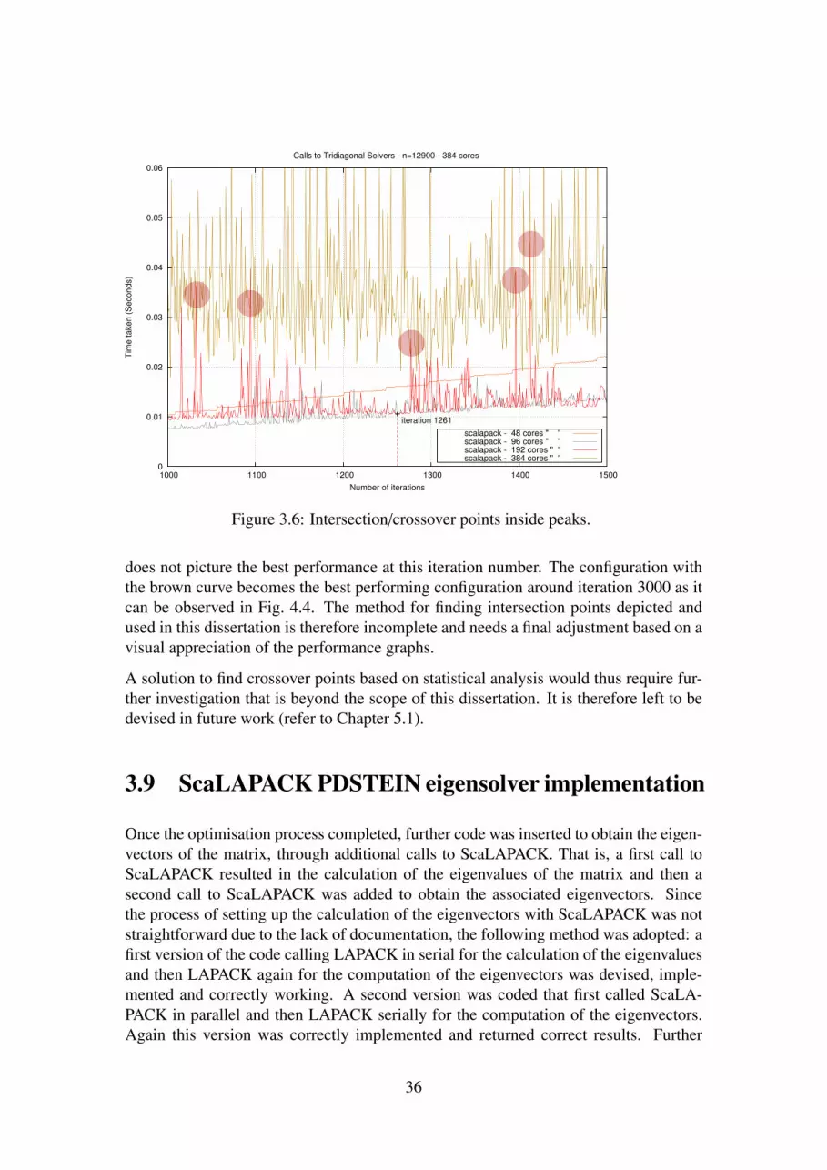
0

0.01

0.02

0.03

0.04

0.05

0.06

1000 1100 1200 1300 1400 1500

Time taken (Seconds)

Number of iterations

Calls to Tridiagonal Solvers - n=12900 - 384 cores 

scalapack -  48 cores "  " scalapack -  96 cores "  " scalapack -  192 cores "  " scalapack -  384 cores "  " 

iteration 1261

Figure 3.6: Intersection/crossover points inside peaks.

does not picture the best performance at this iteration number. The configuration withthe brown curve becomes the best performing configuration around iteration 3000 as itcan be observed in Fig. 4.4. The method for finding intersection points depicted andused in this dissertation is therefore incomplete and needs a final adjustment based on avisual appreciation of the performance graphs.

A solution to find crossover points based on statistical analysis would thus require fur-ther investigation that is beyond the scope of this dissertation. It is therefore left to bedevised in future work (refer to Chapter 5.1).

3.9 ScaLAPACK PDSTEIN eigensolver implementation

Once the optimisation process completed, further code was inserted to obtain the eigen-vectors of the matrix, through additional calls to ScaLAPACK. That is, a first call toScaLAPACK resulted in the calculation of the eigenvalues of the matrix and then asecond call to ScaLAPACK was added to obtain the associated eigenvectors. Sincethe process of setting up the calculation of the eigenvectors with ScaLAPACK was notstraightforward due to the lack of documentation, the following method was adopted: afirst version of the code calling LAPACK in serial for the calculation of the eigenvaluesand then LAPACK again for the computation of the eigenvectors was devised, imple-mented and correctly working. A second version was coded that first called ScaLA-PACK in parallel and then LAPACK serially for the computation of the eigenvectors.Again this version was correctly implemented and returned correct results. Further

36

work would involve completing a third version that uses ScaLAPACK in both calls, torespectively solve the eigenvalues and the eigenvectors of the matrix (see Chapter 5.1).

A few indications that were collected during the initial research about ScaLAPACKPDSTEIN will however be included in this section.

1 s u b r o u t i n e PDSTEBZ ( ICTXT , RANGE, ORDER, N, VL, VU, IL , IU ,ABSTOL, D, E , M, NSPLIT , W, IBLOCK , ISPLIT , WORK, LWORK, IWORK,LIWORK, INFO )

2 s u b r o u t i n e PDSTEIN (N, D, E , M, W, IBLOCK , ISPLIT , ORFAC, Z , IZ ,JZ , DESCZ , WORK, LWORK, IWORK, LIWORK, IFAIL , ICLUSTR , GAP, INFO )

Listing 3.5: PDSTEBZ and PDSTEIN ScaLAPACK subroutines signatures.

Given its signature, the subroutine PDSTEIN expects the parameter ’ORDER’ to be setto ’B’ when calling PDSTEBZ (for more details see [5]). It indicates the order in whichthe eigenvalues and the split-off blocks are to be stored and how they are ordered insidetheses blocks; they are stored from smallest to largest inside each block.

The parameter W corresponds to the array that will contain all the eigenvalues on output.When calling subroutine PDSTEIN, the array W must contain the eigenvalues outputby PDSTEBZ; this translates in placing the two routines successively in the code, theoutput of one feeding the input of the other. In both cases, the vectors D and E areobtained by the Lánczos iteration and correspond to the sets of alphas and betas output(or the diagonal and sub-diagonal elements of matrix T ).

PDSTEIN uses inverse iteration to find some or all the eigenvalues of a tridiagonal ma-trix T. The inverse iteration may incur large dot products when no re-orthogonalisationis selected.

As already mentionned the complete implementation of PDSTEIN is left for futurework.

3.10 Process mapping and core affinity

During the creation of MPI subcommunicators and BLACS contexts, a verification wascarried to assess how the mapping of MPI processes to the underlying hardware wasachieved by the MPI library. This investigation was performed on ARCHER sinceMorar does not allow high numbers of cores. Furthermore, the allocation of MPI pro-cesses to hardware nodes is much more straightforward on ARCHER, because of thepossible adjustments that can be defined in the submission script. For instance, thenumber of processes per node or the number of processes per NUMA region within acore can be initially setup by means of flags given to the program [1].

Due to data locality, process placement can greatly affect performance, MPI processesthat communicate with one another should be placed within the same processor region.Using the MPI subroutine MPI_Get_processor_name and Linux sched_setaffinity and

37

sched_getaffinity API, it was determined how the MPI processes employed in the sub-communicators were mapped to hardware processors. The system call sched_getaffinity()also returns the core affinity of the MPI process that calls it. For results and more detailsrefer to Sections 4.6 and 4.7.

This last investigation closes the chapter covering the whole methodology employedduring the implementation of the different pieces of code and the corresponding inves-tigations or analyses. The next chapter will present in a detailed manner the resultsobtained throughout the whole project since the early stages of the implementation ofthe parallel power method to the investigation concerning the mapping of processes toprocessor cores.

38

Chapter 4

Results and analysis

This chapter presents the results achieved during the whole process of implementing acomplete eigensolver. It covers the initial preparatory phase during which the powermethod was implemented and tested, both in its replicated and distributed forms, theparallel implementation of the Lánczos method and the final step involving the tridi-agonal solvers. In addition to exposing the results obtained during the developmentphases, this chapter also describes an initial analysis of the outcomes of optimising thecalls to the tridiagonal solvers and of the placement of MPI processes on processorsduring the creation of MPI sub-communicators.

Testing was initially performed with small matrices sizes and small number of coresuntil the good functioning of the programs was ensured and then gradually, these pa-rameters were increased to test the robustness and the scalability of the codes.

4.1 Verification with Octave

In order to assess the correctness of the first implementations of the parallel powermethod, both replicated and distributed (see Section 3.3), and of the parallel Lánczosmethod (see Section 3.5), the results of the calculations obtained by the two programswere verified with the help of GNU Octave [12]. GNU Octave is a high-level pro-gramming language aimed at mathematical problems and its syntax is similar to thatof Matlab [16], which makes code portable between both. Octave is Open Source forUnix/Linux operating systems and available as free software.

The execution of the first programs was tested by checking intermediary results duringthe iterations. The values of the variables involved have been verified at certain pointsof the execution. In the case of the power method, the values of the approximation of thedominant eigenvalue, λ, were checked at every iteration for small matrices sizes with4 or 8 elements. In the case of the Lánczos algorithm, the values of the diagonal andsub-diagonal elements of the resulting tridiagonal matrix, the α’s and β’s, were checkedfor correctness, also at each iteration.

39

Diagonal matrices were used to perform the tests since they are much simpler to handlethan normal ones. The eigenvalues of a diagonal matrix are easily predictable sincethese correspond to the diagonal elements of this same matrix [37]. Although thisverification process was carried out with trivial diagonal matrices of very small sizes, itcan be generalised to more complex matrices since the procedure will the same. What isimportant here is to prove the correctness of this implementation of the Lánczos methodthat will be applied to more much more complex matrices. Diagonal matrices are justused for testing purposes.

Existing Matlab code was obtained from Dr. Axel Ruhe from the School of ComputerScience and Communication of the KTH Royal Institute of Technology of Sweden [29]and from the Department of Computational and Applied Mathematics (CAMM) of RiceUniversity [33]. These Matlab programs were then used in the verifications with subse-quent modifications where needed. Again, each variable utilised in the several programswas verified at each iteration against the results output by Octave. In other words, thesame algorithms and the same sequence of operations were run on two different pro-grams with two different languages with the certainty that one was correct. This methodhelped to verify mathematical operations such as vectors dot products, matrix-vectormultiplications, etc. and to pinpoint the location of bugs in the code; this process ofconstant debugging and verification thus ensured and guaranteed the proper function-ing of the present implementations since the initial steps.

Once the codes for both the power method and the Lánczos algorithm were debuggedand correctly compiling, several execution tests were carried out on Morar with smallnumbers of processors. The tests were performed with 2, 4 and 8 cores gradually in-creasing the number of cores to assess the robustness of the programs. A series of initialtests were next executed on ARCHER once the code was running properly on Morar.The results obtained this initial stages are covered in the next sections.

4.2 Power method initial results

The current project started with a given power method serial code that was adapted torun in parallel. Instructions were included in the source code to output the eigenvalueλ and the residual error ||Av − λv|| the algorithm were finding while iterating (see 1 forbackground).

As a simple example, it can be verified in Table. 4.1 that the replicated power methodcorrectly outputs a single eigenvalue λ and an associated eigenvector v(k) when it hasconverged. This single value corresponds to the dominant eigenvalue of matrix A, herewith a very small size of 6 elements, and partitioned into Aloc over 2 processors onMorar. As an another example, with a matrix size of 48 on 48 processors tested onARCHER, as illustrated in Figure 4.1, the value of the eigenvalue found by the powermethod can be seen to converge to the true value of λ1 over 100 iterations as the resid-ual error ||Av − λv|| 4.2 converges towards zero; both values were obtained with the

40

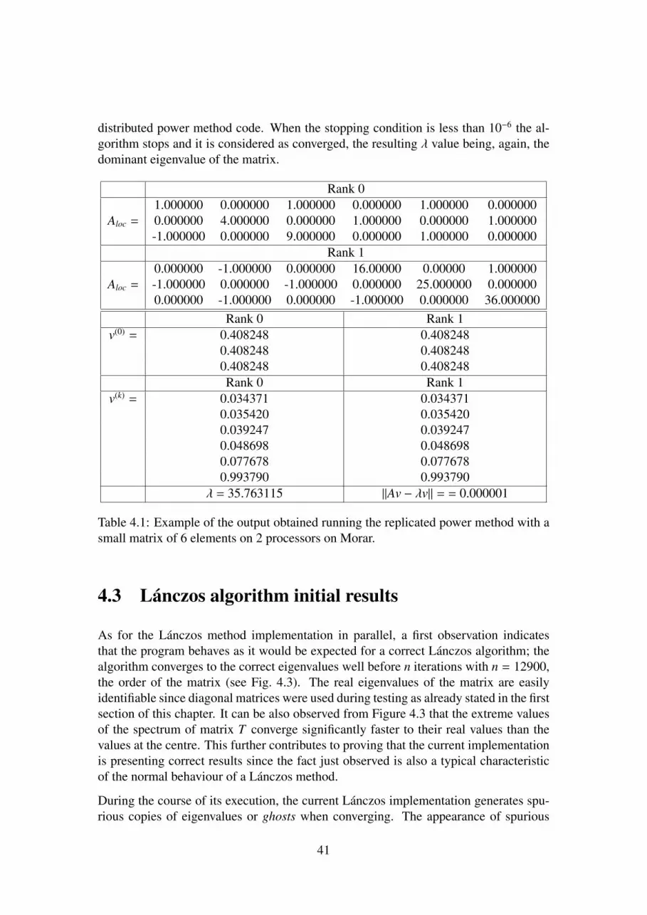
distributed power method code. When the stopping condition is less than 10−6 the al-gorithm stops and it is considered as converged, the resulting λ value being, again, thedominant eigenvalue of the matrix.

Rank 01.000000 0.000000 1.000000 0.000000 1.000000 0.000000

Aloc = 0.000000 4.000000 0.000000 1.000000 0.000000 1.000000-1.000000 0.000000 9.000000 0.000000 1.000000 0.000000

Rank 10.000000 -1.000000 0.000000 16.00000 0.00000 1.000000

Aloc = -1.000000 0.000000 -1.000000 0.000000 25.000000 0.0000000.000000 -1.000000 0.000000 -1.000000 0.000000 36.000000

Rank 0 Rank 1v(0) = 0.408248 0.408248

0.408248 0.4082480.408248 0.408248Rank 0 Rank 1

v(k) = 0.034371 0.0343710.035420 0.0354200.039247 0.0392470.048698 0.0486980.077678 0.0776780.993790 0.993790

λ = 35.763115 ||Av − λv|| = = 0.000001

Table 4.1: Example of the output obtained running the replicated power method with asmall matrix of 6 elements on 2 processors on Morar.

4.3 Lánczos algorithm initial results

As for the Lánczos method implementation in parallel, a first observation indicatesthat the program behaves as it would be expected for a correct Lánczos algorithm; thealgorithm converges to the correct eigenvalues well before n iterations with n = 12900,the order of the matrix (see Fig. 4.3). The real eigenvalues of the matrix are easilyidentifiable since diagonal matrices were used during testing as already stated in the firstsection of this chapter. It can be also observed from Figure 4.3 that the extreme valuesof the spectrum of matrix T converge significantly faster to their real values than thevalues at the centre. This further contributes to proving that the current implementationis presenting correct results since the fact just observed is also a typical characteristicof the normal behaviour of a Lánczos method.

During the course of its execution, the current Lánczos implementation generates spu-rious copies of eigenvalues or ghosts when converging. The appearance of spurious

41

1600

1700

1800

1900

2000

2100

2200

2300

2400

0 20 40 60 80 100

Mag

nitu

de

Iterations

Power method convergence - n=48 - 48 cores

eigenvalues

Figure 4.1: Convergence of the eigenvalue found by the power method code towardsthe real dominant eigenvalue (λreal = 2304.000000) of matrix A, of size 48 × 48 during100 iterations.

0

50

100

150

200

250

300

350

400

450

500

550

0 20 40 60 80 100

Mag

nitu

de

Iterations

Power method convergence - n=48 - 48 cores

||Av-lambda v||

Figure 4.2: Convergence of the residual error ||Av− λv|| towards 0 during 100 iterationsof the power method code (replicated and distributed), with a matrix A of size 48 × 48(λreal = 2304.000000).

42

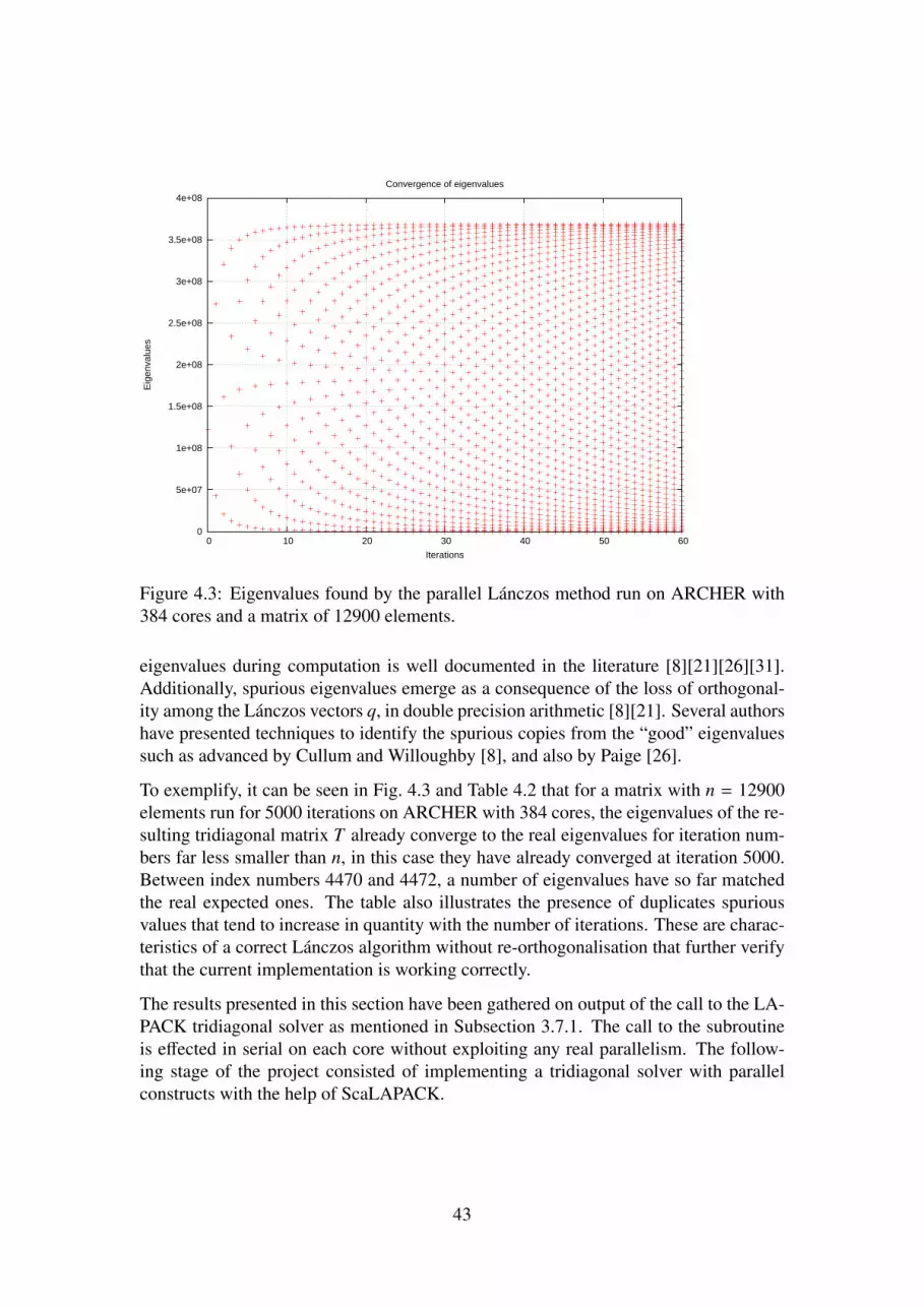
0

5e+07

1e+08

1.5e+08

2e+08

2.5e+08

3e+08

3.5e+08

4e+08

0 10 20 30 40 50 60

Eig

enva

lues

Iterations

Convergence of eigenvalues

Figure 4.3: Eigenvalues found by the parallel Lánczos method run on ARCHER with384 cores and a matrix of 12900 elements.

eigenvalues during computation is well documented in the literature [8][21][26][31].Additionally, spurious eigenvalues emerge as a consequence of the loss of orthogonal-ity among the Lánczos vectors q, in double precision arithmetic [8][21]. Several authorshave presented techniques to identify the spurious copies from the “good” eigenvaluessuch as advanced by Cullum and Willoughby [8], and also by Paige [26].

To exemplify, it can be seen in Fig. 4.3 and Table 4.2 that for a matrix with n = 12900elements run for 5000 iterations on ARCHER with 384 cores, the eigenvalues of the re-sulting tridiagonal matrix T already converge to the real eigenvalues for iteration num-bers far less smaller than n, in this case they have already converged at iteration 5000.Between index numbers 4470 and 4472, a number of eigenvalues have so far matchedthe real expected ones. The table also illustrates the presence of duplicates spuriousvalues that tend to increase in quantity with the number of iterations. These are charac-teristics of a correct Lánczos algorithm without re-orthogonalisation that further verifythat the current implementation is working correctly.

The results presented in this section have been gathered on output of the call to the LA-PACK tridiagonal solver as mentioned in Subsection 3.7.1. The call to the subroutineis effected in serial on each core without exploiting any real parallelism. The follow-ing stage of the project consisted of implementing a tridiagonal solver with parallelconstructs with the help of ScaLAPACK.

43

Eigenvalue index Computed Eigenvalue Real Eigenvalue4467 357512463.999997 357512464.0000004468 357550280.999999 357550281.0000004469 357588099.999999 357588100.0000004470 357625921.000000 357625921.0000004471 357663744.000000 357663744.0000004472 357701569.000000 357701569.000000. . . . . . . . .4919 368140969.000000 368140969.0000004920 368140969.000000 368140969.0000004921 368179178.638291 368179344.0000004922 368179344.000000 368179344.000000. . . . . . . . .

4929 368217721.000000 368217721.0000004930 368217721.000000 368217721.000000. . . . . . . . .

4931 368256099.999999 368256100.0000004932 368256100.000000 368256100.0000004933 368256100.000000 368256100.000000. . . . . . . . .

4994 368640000.000000 368640000.0000004998 368640000.000000 368640000.0000004999 368640000.000000 368640000.0000005000 368640000.000000 368640000.000000

Table 4.2: Spurious eigenvalues found with the Lánczos algorithm run for 5000 iter-ations with a matrix of 12900 × 12900. The dots (. . .) mean that values have beenomitted for clarity. Separators (lines) mean that a change occurs in the value of the realeigenvalue.

4.4 Investigation of the BLACS contexts

In the early stages of the project, the eigenvalues were calculated through a call to theLAPACK DSTEV subroutine which executed the tridiagonal solver at the end of theLánczos iteration. LAPACK is a library that works serially on each core: no exchangeof data occurs between processes at any time and no real parallelism is exploited. Thenext stage of the dissertation was to replace the call to the LAPACK serial solver by acall to ScaLAPACK in parallel.

In order to run ScaLAPACK in parallel, a series of preliminary steps must be performed.A grid of processes must be initially defined so that all the processes included in thegrid will be responsible for the parallelisation of the solver. Various experimentationswith the grid layout of processes have been carried out to investigate the behaviour ofthe tridiagonal solver. In this section, the results of this investigation are exposed. A

44

comparison between the several layout configurations is also included.

To carry out the investigation, the code was profiled by measuring the time taken bythe calls to the tridiagonal solvers. By inserting MPI_Wtime constructs in the code,the durations of the calls to LAPACK and ScaLAPACK were measured and compared.Initially, the matrix size was set to n = 12900 elements and the code was executedwith a total of 384 cores on ARCHER. Several MPI sub-communicators were createdin advance with different sizes: in particular, 6, 12, 24, 48, 96, 192, and 384 cores (seeMethodology 3.7.5). That is, the call to ScaLAPACK subroutine PDSTEBZ was givenin turns a different BLACS context with an associated MPI sub-communicator withvarying size (see Subsection 3.7.3). As pictured in Fig. 4.4 and Fig. 4.5, the behaviourof the call to the solver was directly affected by the number of cores assigned to theBLACS context. In both graphs, the call to LAPACK DSTEV subroutine performedwith the best timing for low numbers of iterations, ranging from 0 to 215. It followsthat a call to the ScaLAPACK subroutine PDSTEBZ with a layout of 24 processesper BLACS context and MPI sub-communicator exhibited the best performance fora very small number of iterations, more specifically between 215 and 264 iterations.Next, it can be observed that a configuration with 48 processes per context showed thebest timings between 552 and 1261 iterations, and between 1261 and 3036 iterationsa BLACS grid with 96 processes was the most performing. Finally, it appears that inFig. 4.4 the lowest time between 3036 and 5000 iterations was obtained assigning 384cores to a single BLACS context and its MPI sub-communicator.

Having defined the performance curves of the several sub-communicators, it is evidentthat the intersections between them define the points where a different configurationperform better. Therefore, the crossover points in Figs 4.6 and 4.7 represent the pointswhere a change of performance occurred and were of vital importance for the nextstages of this research. Based on these observations, the following step was to optimisethe calls to the tridiagonal solvers by switching in a different sub-communicator with adifferent numbers of processes, at these iteration numbers, as previously mentioned.

4.5 Tridiagonal solver optimisation

When the ScaLAPACK solver was first implemented, a single BLACS context wascreated and utilized to execute the solver. However, taking into consideration the pre-vious observations and considerations about best performance when varying BLACScontexts, a number of instructions were inserted in the code that allowed switching thecontext being used to another context that performed with better timings. The switch-ing occurred at well defined iteration numbers, for example, before iteration 215 thecall to the tridiagonal solver was made through the subroutine DSTEV in the LAPACK;at iteration 215, the code switched to a ScaLAPACK configuration that made use of 24cores per sub-communicator, etc. Thus recalling Table 3.1, it can now be modified andextended to include the iteration number at which the switching was carried out (seeTable 4.3).

45

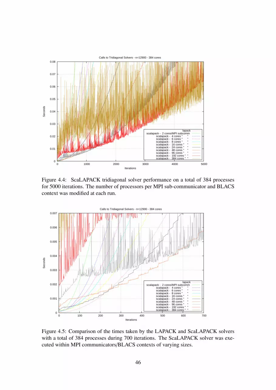
0

0.01

0.02

0.03

0.04

0.05

0.06

0.07

0.08

0 1000 2000 3000 4000 5000

Sec

onds

Iterations

Calls to Tridiagonal Solvers - n=12900 - 384 cores

lapackscalapack - 2 cores/MPI subcomm

scalapack - 4 cores " " scalapack - 6 cores " " scalapack - 8 cores " " scalapack - 16 cores " " scalapack - 24 cores " " scalapack - 48 cores " " scalapack - 96 cores " " scalapack - 192 cores " " scalapack - 384 cores " "

Figure 4.4: ScaLAPACK tridiagonal solver performance on a total of 384 processesfor 5000 iterations. The number of processors per MPI sub-communicator and BLACScontext was modified at each run.

0

0.001

0.002

0.003

0.004

0.005

0.006

0.007

0 100 200 300 400 500 600 700

Sec

onds

Iterations

Calls to Tridiagonal Solvers - n=12900 - 384 cores

lapackscalapack - 2 cores/MPI subcomm

scalapack - 4 cores " " scalapack - 6 cores " " scalapack - 8 cores " " scalapack - 16 cores " " scalapack - 24 cores " " scalapack - 48 cores " " scalapack - 96 cores " " scalapack - 192 cores " " scalapack - 384 cores " "

Figure 4.5: Comparison of the times taken by the LAPACK and ScaLAPACK solverswith a total of 384 processes during 700 iterations. The ScaLAPACK solver was exe-cuted within MPI communicators/BLACS contexts of varying sizes.

46

0

0.0005

0.001

0.0015

0.002

0.0025

0.003

200 250 300 350 400

Sec

onds

Iterations

Calls to Tridiagonal Solvers - n=12900 - 384 cores

lapackscalapack - 2 cores/MPI subcomm

scalapack - 4 cores " " scalapack - 6 cores " " scalapack - 8 cores " " scalapack - 16 cores " " scalapack - 24 cores " " scalapack - 48 cores " " scalapack - 96 cores " " scalapack - 192 cores " " scalapack - 384 cores " "

iteration 215

iteration 264

Figure 4.6: Crossover points at the intersections between the timing curves obtainedrunning LAPACK serially on all the cores and ScaLAPACK in parallel with 24 and 48cores per sub-communicator. These points show that a different number of cores perBLACS context or MPI communicator should be utilised.

0

0.01

0.02

0.03

0.04

0.05

500 1000 1500 2000 2500 3000 3500 4000

Sec

onds

Iterations

Calls to Tridiagonal Solvers - n=12900 - 384 cores

lapackscalapack - 2 cores/MPI subcomm

scalapack - 4 cores " " scalapack - 6 cores " " scalapack - 8 cores " " scalapack - 16 cores " " scalapack - 24 cores " " scalapack - 48 cores " " scalapack - 96 cores " " scalapack - 192 cores " " scalapack - 384 cores " "

iteration 552

iteration 1261

iteration 3036

Figure 4.7: Performance obtained running ScaLAPACK within MPI communica-tors/BLACS contexts with 48, 96, 192 and 384 cores. The crossover points show theintersections between the several timings curves.

47

Iteration number Total numberof groups

Total number ofScaLAPACK instances

Number ofprocesses per group

0 384 384 (LAPACK) 1215 16 16 24264 8 8 48552 4 4 961261 2 2 1923036 1 1 384

Table 4.3: Iteration numbers at which a new MPI sub-communicator was started witha different number of processes, including the resulting numbers of subgroups and ofScaLAPACK instances. LAPACK was used for low numbers of iterations, from itera-tion 0 to 215.

The swapping of BLACS context and MPI sub-communicators has resulted in someimprovement of the performance of the library calls as illustrated in Fig. 4.8. The graphobtained from this new setup demonstrates that the tridiagonal solvers are now perform-ing, at all times, with the best timings obtained during testing. Fig. 4.8 compares theoverall performance of the optimised code (with context switching) with the code usingLAPACK. It clearly shows that any ScaLAPACK version, including the optimised ver-sion, performs significantly better than the version with the LAPACK call, as expected.In addition, it can be observed that the optimised version presents better timings thanany version of ScaLAPACK with a fixed number of cores allocated to the BLACS con-text; this is specially true for low numbers of iterations. However, at some point, sayaround 2800 iterations, both curves of the optimised version and that with 384 cores persub-communicator follow each other closely.

For completeness, Fig. 4.8 further displays that the optimised version (including BLACScontext swapping) behaves significantly better than the version that called the serial LA-PACK subroutine. The gap between the two versions tend to increase much further asthe number of iterations rises. On the other hand, when running the program with highernumbers of cores, for instance 4800 cores, the version that calls LAPACK proved to bethe more efficient for low numbers of iterations than running ScaLAPACK as visiblein Fig. 4.12. This last fact brings further evidence that ScaLAPACK does not handlewell low problem sizes during low numbers of iterations while the matrix T has not yetattained some significant size left for now as arbitrary. The calculation of the minimumsize for the matrix to be efficiently processed by ScaLAPACK in parallel could be leftas an exercise for future work.

The outcome of the optimisation process applied to the tridiagonal solvers is picturedin Fig. 4.9, which clearly demonstrates that the curve of the optimised version of thecode (dark red) was following those with the best timings. Additionally, Fig. 4.10illustrates the performance of several sections of the optimised code: the purple curveshows the time taken by the whole Lánczos iteration including the call to ScaLAPACKPDSTEBZ; the red curve show the time taken by the call to the ScaLAPACK alone; the

48

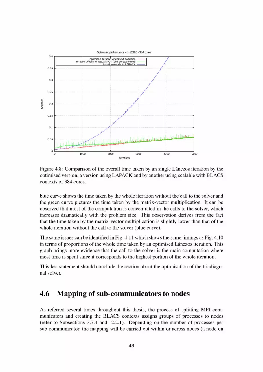
0

0.05

0.1

0.15

0.2

0.25

0.3

0.35

0.4

0 1000 2000 3000 4000 5000

Sec

onds

Iterations

Optimised performance - n=12900 - 384 cores

optimised iteration w/ context switchingiteration w/calls to scaLAPACK (384 cores/context)

iteration w/calls to LAPACK

Figure 4.8: Comparison of the overall time taken by an single Lánczos iteration by theoptimised version, a version using LAPACK and by another using scalable with BLACScontexts of 384 cores.

blue curve shows the time taken by the whole iteration without the call to the solver andthe green curve pictures the time taken by the matrix-vector multiplication. It can beobserved that most of the computation is concentrated in the calls to the solver, whichincreases dramatically with the problem size. This observation derives from the factthat the time taken by the matrix-vector multiplication is slightly lower than that of thewhole iteration without the call to the solver (blue curve).

The same issues can be identified in Fig. 4.11 which shows the same timings as Fig. 4.10in terms of proportions of the whole time taken by an optimised Lánczos iteration. Thisgraph brings more evidence that the call to the solver is the main computation wheremost time is spent since it corresponds to the highest portion of the whole iteration.

This last statement should conclude the section about the optimisation of the triadiago-nal solver.

4.6 Mapping of sub-communicators to nodes

As referred several times throughout this thesis, the process of splitting MPI com-municators and creating the BLACS contexts assigns groups of processes to nodes(refer to Subsections 3.7.4 and 2.2.1). Depending on the number of processes persub-communicator, the mapping will be carried out within or across nodes (a node on

49

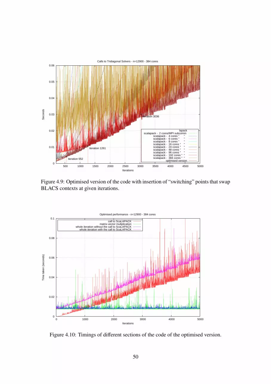
0

0.01

0.02

0.03

0.04

0.05

0.06

500 1000 1500 2000 2500 3000 3500 4000 4500 5000

Sec

onds

Iterations

Calls to Tridiagonal Solvers - n=12900 - 384 cores

lapackscalapack - 2 cores/MPI subcomm

scalapack - 4 cores " " scalapack - 6 cores " " scalapack - 8 cores " " scalapack - 16 cores " " scalapack - 24 cores " " scalapack - 48 cores " " scalapack - 96 cores " " scalapack - 192 cores " " scalapack - 384 cores " "

optimised version iteration 552

iteration 1261

iteration 3036

Figure 4.9: Optimised version of the code with insertion of “switching” points that swapBLACS contexts at given iterations.

0

0.02

0.04

0.06

0.08

0.1

0 1000 2000 3000 4000 5000

Tim

e ta

ken

(sec

onds

)

Iterations

Optimised performance - n=12900 - 384 cores

call to ScaLAPACKmatrix-vector multplication

whole iteration without the call to ScaLAPACKwhole iteration with the call to ScaLAPACK

Figure 4.10: Timings of different sections of the code of the optimised version.

50

0

0.02

0.04

0.06

0.08

0.1

0.12

100200

300400

500600

700800

9001000

11001200

13001400

15001600

17001800

19002000

21002200

23002400

25002600

27002800

29003000

31003200

33003400

35003600

37003800

39004000

41004200

43004400

45004600

47004800

49005000

Sec

onds

Iterations

Time taken by several parts of a single Lanczos iteration - n=12900/384 cores

calls to solversmatrix-vector mult

iteration w/o calls to solvers

Figure 4.11: Proportions taken by the different parts of the code of the optimised ver-sion.

0

0.05

0.1

0.15

0.2

0.25

0.3

0.35

0 20 40 60 80 100

Tim

e ta

ken

(sec

onds

)

Iterations

Calls to Tridiagonal Solvers - n=12900 - 4800 cores

lapackscalapack - 24 cores " " scalapack - 48 cores " " scalapack - 96 cores " "

scalapack - 192 cores " " scalapack - 384 cores " "

scalapack - 4800 cores " "

Figure 4.12: Performance obtained for single instance of scalable running on 4800 corescompared with previous timings obtained with lesser cores.

51

ARCHER has 24 cores at the time of this dissertation). For instance, in the case ofsub-communicators with 12 processes, the MPI library will allocate half a node to eachgroup; a single computational node will execute 2 sub-communicators. In the case ofsub-communicators with 24 cores, a whole node of 24 cores will be allocated to thewhole communicator. For a communicator of 48 processes, 2 nodes will be assigned tothe MPI communicator, etc.

The C functions in the current Lánczos implementation that split MPI communicators(see Listings 3.4) and create the BLACS contexts (see Listings 3.3) also assign new MPIranks valid within the sub-communicator and the new BLACS context. The originalMPI rank attributed by MPI_Comm_rank still maintains within MPI_COMM_WORLDand a second rank identifies the process within the sub-group. Table 4.4 shows the resultof the mapping: the first column represent the original MPI process rank; the secondcolumn shows the newly attributed sub-rank within the sub-communicator; the columnsrow and col show the position within the grid of processes used for ScaLAPACK andpreviously mentioned (refer to Subsection 2.3.4). Since the ScaLAPACK decomposi-tion chosen for this project was one-dimensional, the row column always shows a valueof 0 (first row). It should be noted that rows and columns are numbered by the BLACSfrom 0 to n.

Table 4.4, illustrates the results obtained for a total of 96 processes divided into scal-able sub-communicators with 24 processes each and the corresponding BLACS contextwhich they belong to. The table pictures process 0 to 23 being mapped to context 0 to 3(96 processes / 24 cores per sub-communicator), to the unique row of the process grid(row position 0) and to a column position ranging from 0 to 23. Some lines in the tablewere omitted for simplicity.

MPI rank subrank row col context MPI rank subrank row col context0 0 0 0 0 48 0 0 0 21 1 0 1 0 49 1 0 1 2... ... ... ... ... ... ... ... ... ...22 22 0 22 0 70 22 0 22 223 23 0 23 0 71 23 0 23 224 0 0 0 1 72 0 0 0 325 1 0 1 1 73 1 0 1 3... ... ... ... ... ... ... ... ... ...46 22 0 22 1 94 22 0 22 347 23 0 23 1 95 23 0 23 3

Table 4.4: Mapping of 96 MPI processes onto a BLACS layout grid of 24 processes.The dots (...) mean some that lines have been omitted for clarity and separators (lines)divide BLACS contexts.

In addition, Table 6.1 shows a second example run with 96 cores but with sub-communicatorsof 48 processes. In this case, only 2 contexts have been created, each with 48 processesmapped onto a one-dimensional grid of processes and whose column positions range

52

from 0 to 47, within a single row.

MPI rank subrank row col context MPI rank subrank row col context0 0 0 0 0 48 0 0 0 11 1 0 1 0 49 1 0 1 1... ... ... ... ... ... ... ... ... ...22 22 0 22 0 70 22 0 22 123 23 0 23 0 71 23 0 23 124 0 0 24 0 72 0 0 24 125 1 0 25 0 73 1 0 25 1... ... ... ... ... ... ... ... ... ...46 22 0 46 0 94 22 0 46 147 23 0 47 0 95 23 0 47 1

Table 4.5: Mapping of 96 MPI processes onto a BLACS grid layout of 48 processes.The dots (...) mean that some lines have been omitted for clarity and separators (lines)divide BLACS contexts.

4.7 MPI processes affinity

During the mapping of MPI processes to sub-communicator, described in the previoussection, the MPI subroutine MPI_Get_processor_name was used to verify that BLACScontext were correctly being created and how they were being allocated to hardwarenodes. This section shows the results obtained employing MPI_Get_processor_nameand further ones with the cpusets mechanism (see Appendix A.5, including CPU affin-ity.

Table 4.6 illustrates the mapping of 96 MPI processes to 4 computational nodes onARCHER. Ranks 0 to 23 are mapped onto node “nid01780”, ranks 24 to 47 to node“nid01949”, ranks 48 to 71 to node “nid02650” and rank 72 to 95 to node “nid03024”.Groups of 24 processes are mapped by the MPI library to each computational node,which corresponds to the default number of cores per node on ARCHER at the moment.It can be seen that the MPI processes are mapped to the 16 cores of each processor in anordered fashion, respecting the boundaries of the NUMA regions (see Fig. 4.13). Theinitial objective of this smaller investigation was to verify that sub-communicators andBLACS contexts were not using cores randomly in a unordered manner across NUMAregions within a processor or even across processors in different nodes.

After further investigation it was found out that the mapping of MPI processes to pro-cessor cores is actually carried out by the ALPS or the Application Level PlacementScheduler and according to Cray’s documentation the default setting binds the pro-cesses or thread per NUMA region [19]. NUMA regions can be exploited to allowallocating more than one application to a computational node. The allocation of threadsor MPI processes can be controlled and modified by cpusets which enable determining

53

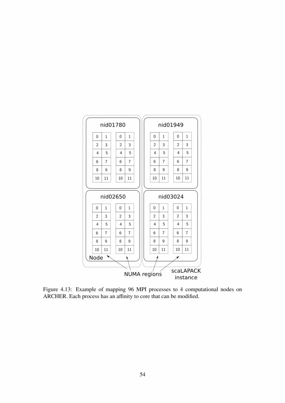
nid01780 nid01949

2

1

3

4 5

6 7

8 9

10 11

0

NUMA regions

Node

scaLAPACKinstance

2

1

3

4 5

6 7

8 9

10 11

0

2

1

3

4 5

6 7

8 9

10 11

0

2

1

3

4 5

6 7

8 9

10 11

0

2

1

3

4 5

6 7

8 9

10 11

0

2

1

3

4 5

6 7

8 9

10 11

0

2

1

3

4 5

6 7

8 9

10 11

0

2

1

3

4 5

6 7

8 9

10 11

0

nid02650 nid03024

Figure 4.13: Example of mapping 96 MPI processes to 4 computational nodes onARCHER. Each process has an affinity to core that can be modified.

54

rank node id core affinity rank node id core affinity0 nid01780 0 48 nid02650 01 nid01780 1 49 nid02650 12 nid01780 2 50 nid02650 23 nid01780 3 51 nid02650 3... ... ... ... ... ...22 nid01780 22 70 nid02650 2223 nid01780 23 71 nid02650 2324 nid01949 0 72 nid03024 025 nid01949 1 73 nid03024 1... ... ... ... ... ...46 nid01949 22 94 nid03024 2247 nid01949 23 95 nid03024 23

Table 4.6: Mapping of 96 MPI processes onto 4 computational nodes on ARCHER.The dots (...) mean that some lines have been omitted for clarity and separators (lines)divide BLACS contexts.

processor and memory placement. More research could be done in this direction, it ishowever left for future work.

55

Chapter 5

Discussion and conclusions

This chapter exposes further ideas developed in previous chapters and tries to bring aconclusion to the findings that were obtained along this dissertation. It mainly coversthe benefits obtained or that could be obtained from swapping MPI sub-communicatorsand BLACS contexts. The chapter also exposes some observations that were made fromthe investigation of the mapping of the MPI processes to hardware cores.

Numerous previous studies have covered the problems presented by the Lánczos algo-rithm. New methods that address these problems have been devised by Parlett and Scott,with a method called LANSO, and more recently, Johnson and Kennedy, with furtherdevelopments to the LANSO, that include selective reorthogonolisation. The currentdissertation has therefore focused on some aspects that have emerged during the studyof the behaviour of the Lánczos method.

The initial idea underlying this project was derived from Johnson and Kennedy’s pa-per [21] and the implementation of a Lánczos method with Chroma [13], a softwarepackage for solving Lattice Quantum Chromodynamics problems. Since Chroma doesnot allow access to lower levels of its functioning such as the communication layers,it was observed that some aspects could not be easily assessed. It was then suggestedthat a Lánczos implementation that offered greater flexibility would be more helpful inunderstanding some of these aspects. Hence, the need for a more flexible Lánczos codethat allowed for instance studying the calculation of the Lánczos vectors or modifyingthe number of cores allocated to the tridiagonal solvers.

After having implemented a correct working Lánczos method in C code, its behaviourwas investigated and its respective performance profiled. Although the project con-cerned the implementation of the Lánczos as a whole, most of the research carried inthis dissertation focused on the implementation of the tridiagonal solver in particular.

It was found that varying numbers of cores in MPI sub-communicators directly af-fected the performance of the tridiagonal solver in ScaLAPACK. Based on these find-ings, a different method was developed that assigns MPI sub-communicators with dif-ferent processes sizes to the parallel tridiagonal solver with the objective to improve

56

its performance. This optimisation takes account of the architecture by creating sub-communicators and communication contexts so that parallel computation can be exe-cuted with memory and locality in mind and minimise expensive remote communica-tions to the strict necessary.

The results exposed in the previous chapters demonstrate that some improvement wasachieved by the optimised code in contrast with a tridiagonal solver that uses 384 coresper sub-communicator, in particular in low iteration counts (refer to Section 4.5 andFig. 4.8). Yet, this small improvement becomes insignificant compared with the wholerange of iterations.

On the other hand, Figs. 4.4 and 4.5 suggest that the performance curves follow a patternacross the whole range of iterations. It is expected that this pattern would continue forhigher numbers of iterations; that beyond 5000 iterations another configuration with alarger number of processes would show better performance. For instance, if the numberof processes is doubled again (768 then 1536 cores), the same pattern would be sup-posed to repeat over 10000 or more iterations. Nevertheless, Fig. 4.12 further demon-strate that high numbers of cores per sub-communicator result in low performance forlow numbers of iterations. It can be observed in Fig. 4.4 that the configuration with 384cores (brown curve) only becomes effective around iteration 3500, thus a configurationwith 1536, 3072 or more cores would also present an increasingly wider initial gap dur-ing which performance is not the best of all. This trend demonstrates that the use ofcontext switching can bring real significant benefits in very large problems with highnumbers of cores, beyond a given number of iterations.

Further work would be necessary to study ways to find the intersection or crossoverpoints between performance curves as stated in Subsection 3.8.1, perhaps using statis-tical analysis. Based on the present research, it is difficult to say a regular mathematicalpattern occurs between the different configurations of processes per sub-communicator.However, a trend can be observed that repeats over the number of iterations. It shouldbe possible to find ways to minimise or completely remove the noise from the perfor-mance curves at least in order to perform calculations; probably by drawing curve fromminima points at least to give a base as to find an existing pattern and maybe extrapolatefuture intersection points.

Concerning the investigation of the mapping of MPI processes to the processor cores, itcan be observed that the mapping respects the “natural” boundaries of NUMA regionsand processors, and that communications and data exchanges are effected by default ina rather optimal way. Nonetheless, the default settings of ARCHER can be altered withflags and options passed to aprun when the program is launched (refer to ARCHER’sonline documentation [1]). Further investigation about the use of the options to aprunshould be carried out to determine how applications such as the present Lánczos methodwould respond to different placements of MPI processes, in terms of performance.

To conclude the section a few last comments were included concerning general pointsnoticed during the present research.

− The eigensolver code is robust and seems to scales smoothly as it was run cor-

57

rectly on 4800 and 9600 cores with a matrix of 12900 double precision elements.

− Since ARCHER is a rather novel computing resource, with less than a year ofexistence, at the moment, it is evident that there is significant room for furtherresearch about exploiting the software and the hardware possibilities that such amachine has to offer.

− During the course of the present project, it was observed that the implementationof the eigensolver would have benefited from a such different choice of program-ming language, such as Fortran instead of C, as the LAPACK and the ScaLA-PACK libraries were coded in Fortran. Many of the problems that appeared dur-ing development may have been due to discrepancies between the two languages.

5.1 Future work

Future work should include a mechanism that compares two data sets containing theperformance timings of the tridiagonal solvers and finds the intersection points or crossoversbetween the two curves using statistical analysis. It also should include the implemen-tation of the ScaLAPACK subroutine PDSTEIN that calculates the eigenvectors of amatrix from the eigenvalues issued from PDSTEBZ also from the ScaLAPACK. Thecreation of the eigenvectors during the Lánczos iteration should also be investigated asit was defined in the initial workplan. Finally, a proper investigation of the flags givento the job scheduler on ARCHER and the corresponding mapping of MPI processes tohardware cores on the processors should be carried out to identify potential performanceimprovements when running groups of processes accross several processors.

58

Appendix A

Source code

A.1 Lánczos Eigensolver

1 / ∗ ∗∗∗∗∗∗∗∗∗∗∗∗∗∗∗∗∗∗∗∗∗∗∗∗∗∗∗∗∗∗∗∗∗∗∗∗∗∗∗∗∗∗∗∗∗∗∗∗∗∗∗∗∗∗∗∗∗∗∗∗∗∗ ∗ /

2 / ∗ p a r a l l e l v e r s i o n o f t h e Lanczos a l g o r i t h m ∗ /

3 / ∗ w i t h c a l l t o a QR s o l v e r i n t h e LAPACK l i b r a r y ∗ /

4 / ∗ − work ing v e r s i o n i n c l u d i n g c a l l t o s c a l a p a c k ∗ /

5 / ∗ − works on morar w / 20 p r o c s w / m a t r i x s i z e n=100 ∗ /

6 / ∗ − p l o t s e i g e n v e c t o r s t o f i l e : o u t . d a t ∗ /

7 / ∗ ( A l g o r i t h m from Paige ) ∗ /

8 / ∗ − USAGE: . / l a n c z o s <numprocs per subcomm> ∗ /

9 / ∗ argument i s t h e number o f p r o c e s s o r s per ∗ /

10 / ∗ MPI subcommunica tor / BLACS c o n t e x t ∗ /

11 / ∗ − I n c l u d e s s w i t c h i n g p o i n t s where BLACS ∗ /

12 / ∗ c o n t e x t s are swapped ∗ /

13 / ∗ Author : Jorge Moreira − 2014 ∗ /

14 / ∗ ( From code s u p p l i e d by C . Johnson ∗ /

15 / ∗ ∗∗∗∗∗∗∗∗∗∗∗∗∗∗∗∗∗∗∗∗∗∗∗∗∗∗∗∗∗∗∗∗∗∗∗∗∗∗∗∗∗∗∗∗∗∗∗∗∗∗∗∗∗∗∗∗∗∗∗∗∗∗∗ ∗ /

1617 # i n c l u d e < s t d i o . h>

18 # i n c l u d e < s t d l i b . h>

19 # i n c l u d e <math . h>

20 # i n c l u d e <mpi . h>

21 # i n c l u d e < a s s e r t . h>

2223 # i f n d e f max24 # d e f i n e max ( a , b ) ( ( ( a ) >(b ) ) ? ( a ) : ( b ) )25 # e n d i f2627 # d e f i n e ORDER 19200 / / 19200 / / m a t r i x and v e c t o r s s i z e28 # d e f i n e RESULTS_FILE " o u t . d a t " / ∗ name o f o u t p u t r e s u l t s f i l e ∗ /

29 # d e f i n e NUMPROCS_PER_NODE 24 / / s i n g l e node on ARCHER30 # d e f i n e NUM_CROSSOVERS 5 / / number o f MPI subcomm / BLACS c o n t e x t s

swaps31 # d e f i n e NUM_ITER 50003233 / ∗ ∗∗∗ P r o t o t y p e s ∗∗∗ ∗ /

A1

34 / ∗ LAPACK ∗ /

35 i n t d s t e v _ ( char ∗ , i n t ∗ , double ∗ , double ∗ , double ∗ , i n t ∗ , double∗ , i n t ∗ ) ;

36 double dlamch_ ( char ∗ ) ;37 / ∗ scaLAPACK ∗ /

38 i n t p d s t e b z _ ( i n t ∗ , char ∗ , char ∗ , i n t ∗ , double ∗ , double ∗ , i n t ∗ ,i n t ∗ ,

39 double ∗ , double ∗ , double ∗ , i n t ∗ , i n t ∗ , double ∗ , i n t ∗ ,i n t ∗ ,

40 double ∗ , i n t ∗ , i n t ∗ , i n t ∗ , i n t ∗ ) ;41 / ∗ Cblacs ∗ /

42 e x t er n void C b l a c s _ p i n f o ( ) ;43 e x t er n void C b l a c s _ g e t ( ) ;44 e x t er n void C b l a c s _ g r i d i n f o ( ) ;45 e x t er n void C b l a c s _ g r i d i n i t ( ) ;46 e x t er n void C b l a c s _ g r i d e x i t ( i n t ) ;47 e x t er n void C b l a c s _ e x i t ( i n t ) ;48 e x t er n void C b l a c s _ s e t u p ( i n t ∗ , i n t ∗ ) ;49 e x t er n void C f r e e _ b l a c s _ s y s t e m _ h a n d l e ( i n t ) ;5051 e x t er n i n t C s y s 2 b l a c s _ h a n d l e ( MPI_Comm) ;5253 / / l o c a l54 i n t c r e a t e _ o u t p u t _ f i l e ( double ∗ , char ∗ , i n t , i n t , i n t , i n t ) ;55 / / v o i d s p l i t _ c o m m u n i c a t o r s (MPI_Comm ∗ , i n t ∗ , i n t ∗ , i n t ) ;56 void s p l i t _ c o m m u n i c a t o r s (MPI_Comm ∗ , i n t ∗ , i n t ∗ ) ;57 / / i n t in i t_BLACS (MPI_Comm ∗ , i n t ∗ , i n t , i n t ) ;58 i n t init_BLACS (MPI_Comm ∗ , i n t ∗ , i n t ∗ ) ;59 double ∗∗ a l l o c a t e _ m a t r i x ( i n t , i n t ) ;60 double ∗ a l l o c a t e _ d v e c t o r ( i n t ) ;61 i n t ∗ a l l o c a t e _ i v e c t o r ( i n t ) ;62 void p o p u l a t e _ m a t r i x ( double ∗∗ , i n t , i n t , i n t , i n t , i n t ) ;63 void p o p u l a t e _ v e c t o r ( double ∗ , i n t ) ;64 double d o t _ p r o d u c t ( double ∗ , double ∗ , i n t ) ;65 void m a t v e c m u l t _ o r i g ( double ∗∗ , i n t , i n t , double ∗ , double ∗ ) ;66 void matvecmul t ( double ∗∗ , i n t , i n t , i n t , double ∗ , double ∗ ) ;67 double L2norm_orig ( double ∗ , i n t ) ;68 double L2norm ( double ∗ , i n t ) ;69 void n o r m a l i s e ( double ∗ , i n t ) ;70 void p r i n t v e c ( double ∗ , i n t ) ;71 void p r i n t m a t ( double ∗∗ , i n t , i n t ) ;72 void f ree_memory ( double ∗∗ , double ∗ , double ∗ , double ∗ , double ∗ ,

double ∗ ,73 double ∗ , double ∗ , double ∗ , double ∗ , double ∗ , double ∗ ,

double ∗ ,74 double ∗ , double ∗ , i n t ∗ , i n t ∗ , i n t ∗ , i n t , i n t ) ;7576 / ∗ F u n c t i o n s ∗ /

77 void p o p u l a t e _ m a t r i x ( double ∗∗ a , i n t n , i n t s p a r s i t y , i n t s t a r t r o w ,i n t numrow ,

78 i n t numcol ) {7980 i n t f r e q ;81

A2

82 f r e q = ( i n t ) ( ( double ) n / ( double ) s p a r s i t y ) ;8384 / / p r i n t f ( " f r e q = %d \ n " , f r e q ) ;8586 f o r ( i n t i = 0 ; i < numrow ; i ++) {87 f o r ( i n t j = i + s t a r t r o w − 1 ; j < numcol ; j = j + f r e q ) {88 a [ i ] [ j ] = 1 . 0 ;89 }90 f o r ( i n t j = i + s t a r t r o w − 1 ; j >= 0 ; j = j − f r e q ) {91 i f ( ( i + s t a r t r o w − 1) == j ) {92 a [ i ] [ j ] = ( i + s t a r t r o w ) ∗ ( i + s t a r t r o w ) ;93 } e l s e {94 a [ i ] [ j ] = −1 .0 ;95 }96 }97 }98 }99

100 void p o p u l a t e _ v e c t o r ( double ∗v , i n t numrow ) {101102 f o r ( i n t i = 0 ; i < numrow ; i ++) {103 v [ i ] = 1 . 0 ;104 }105 }106107 double d o t _ p r o d u c t ( double ∗v , double ∗w, i n t numrow ) {108109 double ans = 0 . 0 ;110 f o r ( i n t i = 0 ; i < numrow ; i ++) {111 ans += v [ i ] ∗ w[ i ] ;112 }113 re turn ans ;114 }115116 void m a t v e c m u l t _ o r i g ( double ∗∗ a , i n t numrow , i n t numcol , double ∗v ,

double ∗w) {117118 f o r ( i n t i = 0 ; i < numrow ; i ++) {119 w[ i ] = 0 . 0 ;120 f o r ( i n t j = 0 ; j < numcol ; j ++) {121 w[ i ] += a [ i ] [ j ] ∗ v [ j ] ;122 }123 }124 }125126 void matvecmul t ( double ∗∗ a , i n t numrow , i n t s t a r t c o l , i n t endco l ,

double ∗v ,127 double ∗w) {128 f o r ( i n t i = 0 ; i < numrow ; i ++) {129 w[ i ] = 0 . 0 ;130 f o r ( i n t j = 0 , k = s t a r t c o l ; k < e n d c o l ; j ++ , k++) {131 w[ i ] += a [ i ] [ k ] ∗ v [ j ] ;132 }133 }

A3

134 }135136 double L2norm_orig ( double ∗v , i n t numrow ) {137138 double norm = 0 . 0 ;139140 norm = d o t _ p r o d u c t ( v , v , numrow ) ;141 norm = s q r t ( norm ) ;142143 re turn norm ;144145 }146147 / ∗ sq ua re r o o t o f t h e d o t p r o d u c t o f two v e c t o r s . ∗ /

148 double L2norm ( double ∗v , i n t numrow ) {149 double norm = 0 . 0 ;150 double p a r t i a l _ n o r m = 0 . 0 ;151152 p a r t i a l _ n o r m = d o t _ p r o d u c t ( v , v , numrow ) ;153 MPI_Al l reduce (& p a r t i a l _ n o r m , &norm , 1 , MPI_DOUBLE, MPI_SUM,

MPI_COMM_WORLD) ;154 norm = s q r t ( norm ) ;155156 re turn norm ;157 }158159 void n o r m a l i s e ( double ∗v , i n t numrow ) {160161 double norm = 0 . 0 ;162 norm = L2norm ( v , numrow ) ;163 f o r ( i n t i = 0 ; i < numrow ; i ++) {164 v [ i ] = v [ i ] / norm ;165 }166 }167168 void p r i n t v e c ( double ∗v , i n t numrow ) {169170 f o r ( i n t i = 0 ; i < numrow ; i ++) {171 p r i n t f ( "%f \ n " , v [ i ] ) ;172 }173 }174175 void p r i n t m a t ( double ∗∗ a , i n t numrow , i n t numcol ) {176177 f o r ( i n t i = 0 ; i < numrow ; i ++) {178 f o r ( i n t j = 0 ; j < numcol ; j ++) {179 p r i n t f ( "%f " , a [ i ] [ j ] ) ;180 }181 p r i n t f ( " \ n " ) ;182 }183 }184185 i n t d s t e v ( char j obs , i n t n , double ∗d , double ∗e , double ∗z , i n t ldz ,186 double ∗work ) {

A4

187188 i n t i n f o ;189 d s t e v _ (& jobs , &n , d , e , z , &ldz , work , &i n f o ) ;190191 re turn i n f o ;192 }193194 i n t p d s t e b z ( i n t i c t x t , char range , char o r d e r , i n t n , double vl ,

double vu ,195 i n t i l , i n t iu , double a b s t o l , double ∗d , double ∗e , i n t m,

i n t n s p l i t ,196 double ∗w, i n t ∗ i b l o c k , i n t ∗ i s p l i t , double ∗work , i n t lwork ,197 i n t ∗ iwork , i n t l i w o r k ) {198 i n t i n f o ;199 p d s t e b z _ (& i c t x t , &range , &o r d e r , &n , &vl , &vu , &i l , &iu , &a b s t o l ,

d , e , &m,200 &n s p l i t , w, i b l o c k , i s p l i t , work , &lwork , iwork , &l iwork ,

&i n f o ) ;201202 re turn i n f o ;203 }204205 double dlamch ( char cmach ) {206 re turn dlamch_(&cmach ) ;207208 }209210 / / Free a l l a l l o c a t e d memory211 void f ree_memory ( double ∗∗ a , double ∗ temp1 , double ∗ temp2 , double ∗

q _ l o c a l ,212 double ∗ r _ l o c a l , double ∗ r _ r e c v , double ∗ r _ p r e v i o u s , double ∗

a lpha ,213 double ∗ be ta , double ∗ a lpha_temp , double ∗ beta_ temp , double ∗

z ,214 double ∗work_lapack , double ∗work_sca l apack , double ∗w, i n t ∗

i b l o c k ,215 i n t ∗ i s p l i t , i n t ∗ iwork , i n t n , i n t numrow ) {216 f o r ( i n t i = 0 ; i < numrow ; i ++) {217 f r e e ( a [ i ] ) ;218 }219 f r e e ( a ) ;220221 f r e e ( temp1 ) ;222 f r e e ( temp2 ) ;223 f r e e ( q _ l o c a l ) ;224 f r e e ( r _ l o c a l ) ;225 f r e e ( r _ r e c v ) ;226 f r e e ( r _ p r e v i o u s ) ;227 f r e e ( a l p h a ) ;228 f r e e ( b e t a ) ;229 f r e e ( a lpha_ temp ) ;230 f r e e ( be t a_ t emp ) ;231 f r e e ( z ) ;232 f r e e ( work_ lapack ) ;

A5

233 f r e e ( w o r k _ s c a l a p a c k ) ;234 f r e e (w) ;235 f r e e ( i b l o c k ) ;236 f r e e ( i s p l i t ) ;237 f r e e ( iwork ) ;238239 }240241 / ∗ A l l o c a t e m a t r i c e s memory ∗ /

242 double ∗∗ a l l o c a t e _ m a t r i x ( i n t numrow , i n t numcol ) {243 double ∗∗ a = ( double ∗∗ ) ma l lo c ( numrow ∗ s i z e o f ( double ∗ ) ) ;244 i f ( a == NULL) {245 f p r i n t f ( s t d e r r , " Out o f memory ( a ) \ n " ) ;246 e x i t ( 8 ) ;247 }248249 f o r ( i n t i = 0 ; i < numrow ; i ++) {250 a [ i ] = ( double ∗ ) m a l lo c ( numcol ∗ s i z e o f ( double ) ) ;251 i f ( a [ i ] == NULL) {252 f p r i n t f ( s t d e r r , " Out o f memory ( a[%d ] ) \ n " , i ) ;253 e x i t ( 8 ) ;254 }255 }256 re turn a ;257 }258259 / ∗ A l l o c a t e d ou b l e v e c t o r s memory ∗ /

260 double ∗ a l l o c a t e _ d v e c t o r ( i n t s i z e ) {261 double ∗v = ( double ∗ ) m a l lo c ( s i z e ∗ s i z e o f ( double ) ) ;262 i f ( v == NULL) {263 f p r i n t f ( s t d e r r , " Out o f memory ( v ) \ n " ) ;264 e x i t ( 8 ) ;265 }266 re turn v ;267 }268269 / ∗ A l l o c a t e i n t e g e r v e c t o r memory ∗ /

270 i n t ∗ a l l o c a t e _ i v e c t o r ( i n t s i z e ) {271 i n t ∗v = ( i n t ∗ ) m a l lo c ( s i z e ∗ s i z e o f ( i n t ) ) ;272 i f ( v == NULL) {273 f p r i n t f ( s t d e r r , " Out o f memory ( v ) \ n " ) ;274 e x i t ( 8 ) ;275 }276 re turn v ;277 }278279 / ∗

∗∗∗∗∗∗∗∗∗∗∗∗∗∗∗∗∗∗∗∗∗∗∗∗∗∗∗∗∗∗∗∗∗∗∗∗∗∗∗∗∗∗∗∗∗∗∗∗∗∗∗∗∗∗∗∗∗∗∗∗∗∗∗∗∗∗∗∗∗∗∗∗∗∗∗∗∗∗

280 ∗

281 ∗ S p l i t t h e u n i v e r a l c o m u n i c a t o r i n t o subcommunica tor s f o r eachs i n g l e node ∗

282 ∗ MPI_comm ∗ subcomm − p o i n t e r t o t h e r e s u l t i n g MPI subcommunica tor∗

A6

283 ∗ i n t ∗ r a n k s − t h e r a n k s b e f o r e ( r a n k s [ 0 ] ) and a f e r t h e s p l i t t i n g (r a n k s [ 1 ] ) ∗

284 ∗ r a n k s [0]= rank number r e t u r n e d by MPI_Comm_rank ,285 ∗ r a n k s [1]= new rank r e t u r n e d by MPI_Comm_split ,286 ∗ i . e . rank i n s i d e a subcommunica tor287 ∗ r a n k s [2]= rank r e t u r n e d by t h e BLACS i n i t i a l i s a t i o n .288 ∗ i n t ∗ numprocs − t h e number o f p r o c e s s o r s a t MPI i n i t and a f t e r t h e

s p l i t t i n g ∗

289 ∗ numprocs [0]= t o t a l number o f p r o c e s s o r s ,290 ∗ numprocs [1]= number o f p r o c e s s e s i n a s i n g l e subcommunica tor291 ∗

292 ∗

∗∗∗∗∗∗∗∗∗∗∗∗∗∗∗∗∗∗∗∗∗∗∗∗∗∗∗∗∗∗∗∗∗∗∗∗∗∗∗∗∗∗∗∗∗∗∗∗∗∗∗∗∗∗∗∗∗∗∗∗∗∗∗∗∗∗∗∗∗∗∗∗∗∗∗∗∗

∗ /

293 void s p l i t _ c o m m u n i c a t o r s (MPI_Comm ∗subcomm , i n t ∗ r anks , i n t ∗ numprocs) {

294 i n t namelen , c o l o u r , num_subcomms , numprocs_per_subcomm ;295 char p r o c e s s o r _ n a m e [MPI_MAX_PROCESSOR_NAME ] ;296 i n t ∗ con tex t_name ;297298 MPI_Get_processor_name ( processo r_name , &namelen ) ;299300 # i f d e f DEBUG301 p r i n t f ( " H e l l o wor ld ! I ’m rank %d of %d on %s \ n " , r a n k s [ 0 ] ,

numprocs [ 0 ] ,302 p r o c e s s o r _ n a m e ) ;303 # e n d i f304305 numprocs_per_subcomm = numprocs [ 1 ] ;306 num_subcomms = numprocs [ 0 ] / numprocs [ 1 ] ;307 con tex t_name = ( i n t ∗ ) m a l lo c ( num_subcomms ∗ s i z e o f ( i n t ) ) ;308 i f ( con tex t_name == NULL) {309 f p r i n t f ( s t d e r r , " Out o f memory ( con tex t_name ) \ n " ) ;310 e x i t ( 8 ) ;311 }312313 f o r ( i n t i = 0 ; i < num_subcomms ; i ++) {314 con tex t_name [ i ] = i ;315 }316317 c o l o u r = r a n k s [ 0 ] / numprocs [ 1 ] ;318 MPI_Comm_split (MPI_COMM_WORLD, c o l o u r , r a n k s [ 0 ] , subcomm ) ;319 MPI_Comm_rank (∗ subcomm , &r a n k s [ 1 ] ) ;320 MPI_Comm_size (∗ subcomm , &numprocs [ 1 ] ) ;321322 # i f d e f DEBUG323 p r i n t f ( " i n s i d e s p l i t %d : I ’m rank %d of %d i n t h e %d c o n t e x t \ n " ,

r a n k s [ 0 ] ,324 r a n k s [ 1 ] , numprocs [ 1 ] , con tex t_name [ c o l o u r ] ) ;325 # e n d i f326327 / / DEBUG328 / / a s s e r t ( numprocs [ 1 ] == numprocs_per_subcomm ) ;329 f r e e ( con tex t_name ) ;

A7

330 }331332 / ∗ S e t up t h e BLACS e n v i r o n m e n t ∗ /

333 i n t init_BLACS (MPI_Comm ∗ sub_communica tor , i n t ∗ r anks , i n t ∗ numprocs ){

334 i n t n r o w s _ p r o c _ g r i d , n c o l s _ p r o c _ g r i d , l o c a l _ r o w _ p o s = 0 ,l o c a l _ c o l _ p o s = 0 ;

335 i n t BLACS_handle , BLACS_context ;336 i n t b l o c k _ s i z e _ p e r _ c o r e ; / / problem s i z e per p r o c e s s337 i n t z e r o = 0 ;338 char o r d e r _ b l a c s = ’R ’ ;339340 BLACS_handle = C s y s 2 b l a c s _ h a n d l e (∗ sub_communica tor ) ;341 BLACS_context = BLACS_handle ; / / can ’ t s k i p t h i s i n t e r m e d i a r y

s t e p ?342343 / / I n i t i a l i s e p a r a m e t e r s344 n r o w s _ p r o c _ g r i d = 1 ; / / number o f rows i n t h e p r o c e s s o r g r i d345 n c o l s _ p r o c _ g r i d = numprocs [ 1 ] ; / / number o f rows i n t h e

p r o c e s s o r g r i d346 b l o c k _ s i z e _ p e r _ c o r e = ORDER / numprocs [ 1 ] ;347 i n t rowxcol = n r o w s _ p r o c _ g r i d ∗ n c o l s _ p r o c _ g r i d ;348349 / / guards f o r e r r o n e o u s i n p u t s i z e s or number o f subcommunica tor s350 i f ( numprocs [ 0 ] < numprocs [ 1 ] ) {351 i f (0 == r a n k s [ 0 ] ) {352 p r i n t f (353 " E x i t : mismatch between t h e number o f p r o c e s s o r s

and t h e number o f p r o c e s s e s p e r subcommunica to r s \ n " ) ;354 p r i n t f ( " Number o f p r o c e s s o r s : %d \ tNumber o f

subcommunica to r s : %d \ n " ,355 numprocs [ 0 ] , numprocs [ 1 ] ) ;356 M P I _ F i n a l i z e ( ) ;357 e x i t ( EXIT_FAILURE ) ;358 }359 }360361 i f ( ( ( ORDER / b l o c k _ s i z e _ p e r _ c o r e ) < n r o w s _ p r o c _ g r i d )362 | | ( (ORDER / b l o c k _ s i z e _ p e r _ c o r e ) < n c o l s _ p r o c _ g r i d ) )363 i f (0 == r a n k s [ 0 ] ) {364 p r i n t f ( " E x i t : problem s i z e t o o s m a l l f o r p r o c e s s o r s e t ! \ n

" ) ;365 M P I _ F i n a l i z e ( ) ;366 e x i t ( EXIT_FAILURE ) ;367 }368369 / ∗ I n i t i a l i s e BLACS ∗ /

370 C b l a c s _ p i n f o (& r a n k s [ 2 ] , &numprocs [ 0 ] ) ;371 i f ( numprocs [ 0 ] < 1)372 C b l a c s _ s e t u p (& r a n k s [ 2 ] , &rowxcol ) ;373374 C b l a c s _ g r i d i n i t (&BLACS_context , &o r d e r _ b l a c s , n r o w s _ p r o c _ g r i d ,375 n c o l s _ p r o c _ g r i d ) ;

A8

376 C b l a c s _ g r i d i n f o ( BLACS_context , &n r o w s _ p r o c _ g r i d , &n c o l s _ p r o c _ g r i d,

377 &l o c a l _ r o w _ p o s , &l o c a l _ c o l _ p o s ) ;378379 # i f d e f DEBUG380 p r i n t f ( " Outpu t f o r p r o c e s s o r %d \ n " , r a n k s [ 2 ] ) ;381 p r i n t f ( "MPI rank %d proc %d i n p r o c e s s o r − a r r a y i s row %d , c o l %d

\ n " , r a n k s [ 0 ] , r a n k s [ 2 ] , l o c a l _ r o w _ p o s , l o c a l _ c o l _ p o s ) ;382 p r i n t f ( "−−−−−−−−\n " ) ;383 # e n d i f384385 i f ( r a n k s [ 2 ] != r a n k s [ 0 ] ) {386 p r i n t f ( " i n c o r r e c t mapping \ n " ) ;387 M P I _ F i n a l i z e ( ) ;388 e x i t ( EXIT_FAILURE ) ;389 }390391 / / B a i l o u t i f t h i s p r o c e s s i s n o t a p a r t o f t h i s c o n t e x t .392 i f (−1 == l o c a l _ c o l _ p o s )393 C b l a c s _ e x i t ( z e r o ) ;394395 re turn BLACS_context ;396 }397398 i n t main ( i n t argc , char ∗ a rgv [ ] ) {399 i n t s t a r t r o w ;400 i n t s p a r s i t y ;401 i n t n , numrow , numcol , l l d ;402403 FILE ∗ fp1 , ∗ fp2 ;404 double ∗∗ a , ∗∗q ;405 double ∗ temp1 , ∗ temp2 , ∗ q _ l o c a l , ∗ r _ l o c a l , ∗ r _ r e c v , ∗ r _ p r e v i o u s ;406407 / ∗ New v a r i a b l e s ∗ /

408 i n t k = 0 ;409 double ∗ a lpha , ∗ be ta , ∗ a lpha_temp , ∗ be t a_ t emp ;410 i n t r i g h t , l e f t , s t a r t c o l , endco l , t ag , t a u ;411 double a l p h a _ l o c a l , a l p h a _ c u r r e n t , b e t a _ c u r r e n t , b e t a _ p r e v i o u s =

0 ;412413 / ∗ LAPACK c a l l v a r i a b l e s ∗ /

414 char j o b s = ’N’ ;415 i n t i n f o = −1 , l d z = 1 ;416 double ∗z , ∗work_ lapack ;417418 / ∗ scaLAPACKS v a r i a b l e s ∗ /

419 i n t ∗ i b l o c k , ∗ i s p l i t ;420 i n t num_eig = 0 , n s p l i t = 0 , lwork , l iwork , ∗ iwork ;421 char r a n g e = ’A’ , o r d e r _ s c a = ’E ’ , mach = ’U’ ;422 double ∗work_sca l apack , ∗w;423 double v l = 0 . 0 , vu = 0 . 0 , i l = 0 . 0 , i u = 0 . 0 , a b s t o l = dlamch (

mach ) ;424425 / ∗ ∗∗∗∗∗∗∗∗∗∗∗∗∗∗∗∗∗∗∗∗∗∗∗∗∗∗∗∗∗∗∗∗∗∗∗∗∗∗∗∗∗∗∗∗∗∗∗∗∗∗∗∗∗∗∗∗∗∗∗∗∗

A9

426 ∗ t o t a l number o f subcommunica tor s427 ∗ ( numprocs / numprocs_per_subcomm )428 ∗ ∗∗∗∗∗∗∗∗∗∗∗∗∗∗∗∗∗∗∗∗∗∗∗∗∗∗∗∗∗∗∗∗∗∗∗∗∗∗∗∗∗∗∗∗∗∗∗∗∗∗∗∗∗∗∗∗∗∗∗∗ ∗ /

429 i n t num_subcomms ;430431 / ∗ ∗∗∗∗∗∗∗∗∗∗∗∗∗∗∗∗∗∗∗∗∗∗∗∗∗∗∗∗∗∗∗∗∗∗∗∗∗∗∗∗∗∗∗∗∗∗∗∗∗∗∗∗∗∗∗∗∗∗∗∗∗∗

432 ∗ number o f p r o c e s s e s per subcommunica tor433 ∗ ( d e f a u l t ==24 − 1 node =24 c o r e s on ARCHER)434 ∗ ∗∗∗∗∗∗∗∗∗∗∗∗∗∗∗∗∗∗∗∗∗∗∗∗∗∗∗∗∗∗∗∗∗∗∗∗∗∗∗∗∗∗∗∗∗∗∗∗∗∗∗∗∗∗∗∗∗∗∗∗ ∗ /

435 i n t numprocs_per_subcomm = NUMPROCS_PER_NODE;436437 / ∗ ∗∗∗∗∗∗∗∗∗∗∗∗∗∗∗∗∗∗∗∗∗∗∗∗∗∗∗∗∗∗∗∗∗∗∗∗∗∗∗∗∗∗∗∗∗∗∗∗∗∗∗∗∗ ∗

438 ∗ r a n k s [0]= rank number r e t u r n e d by MPI_Comm_rank ,439 ∗ r a n k s [1]= new rank r e t u r n e d by MPI_Comm_split ,440 ∗ i . e . rank i n s i d e a subcommunica tor441 ∗ r a n k s [2]= rank r e t u r n e d by t h e BLACS i n i t i a l i s a t i o n .442 ∗ ∗∗∗∗∗∗∗∗∗∗∗∗∗∗∗∗∗∗∗∗∗∗∗∗∗∗∗∗∗∗∗∗∗∗∗∗∗∗∗∗∗∗∗∗∗∗∗∗∗∗∗∗∗ ∗ /

443 i n t r a n k s [ 3 ] ;444445 / ∗ ∗∗∗∗∗∗∗∗∗∗∗∗∗∗∗∗∗∗∗∗∗∗∗∗∗∗∗∗∗∗∗∗∗∗∗∗∗∗∗∗∗∗∗∗∗∗∗∗∗∗∗∗∗∗∗∗∗∗∗∗∗

446 ∗ numprocs [0]= t o t a l number o f p r o c e s s o r s ,447 ∗ numprocs [1]= number o f p r o c e s s e s i n a s i n g l e subcommunica tor448 ∗ ∗∗∗∗∗∗∗∗∗∗∗∗∗∗∗∗∗∗∗∗∗∗∗∗∗∗∗∗∗∗∗∗∗∗∗∗∗∗∗∗∗∗∗∗∗∗∗∗∗∗∗∗∗∗∗∗∗∗∗∗ ∗ /

449 i n t numprocs [ 2 ] ;450451 / ∗ BLACS v a r i a b l e s ∗ /

452 i n t BLACS_handle = −1 , BLACS_context ;453 i n t c u r r e n t _ p r o c , n r o w s _ p r o c _ g r i d , n c o l s _ p r o c _ g r i d , l o c a l _ r o w _ p o s

= 0 ,454 l o c a l _ c o l _ p o s = 0 ;455 i n t b l o c k _ s i z e , z e r o = 0 ;456 char o r d e r _ b l a c s = ’R ’ ;457458 / ∗ MPI v a r i a b l e s ∗ /

459 MPI_Request r e q u e s t 1 , r e q u e s t 2 ;460 MPI_Sta tus s t a t u s ;461 MPI_Comm sub_communica tor ;462463 / ∗ t i m i n g ∗ /

464 double t1 , t2 , t3 , t 4 ;465466 / ∗ s w i t c h e s v a r i a b l e s ∗ /

467 i n t i n d e x = 0 ; / / i n d e x i n a r r a y o f BLACS c o n t e x t s468 i n t ∗BLACS_contexts ;469 i n t num_swi tches = 1 ;470 i n t c o n f i g [NUM_CROSSOVERS] = { 24 , 48 , 96 , 192 , 384 } ;471 i n t c r o s s o v e r s [NUM_CROSSOVERS] = { 215 , 264 , 552 , 1261 , 3036 } ;472473 / ∗ i n i t i a l i s e MPI e n v i r o n m e n t ∗ /

474 M P I _ In i t (& argc , &argv ) ;475 MPI_Comm_size (MPI_COMM_WORLD, &numprocs [ 0 ] ) ;476 MPI_Comm_rank (MPI_COMM_WORLD, &r a n k s [ 0 ] ) ;477478 i f (ORDER % numprocs [ 0 ] ) {

A10

479 i f (0 == r a n k s [ 0 ] )480 p r i n t f (481 "ERROR: numprocs = %d , i t must be a m u l t i p l e o f

t h e m a t r i x s i z e and of 2 4 \ n " ,482 numprocs [ 0 ] ) ;483 {484 M P I _ F i n a l i z e ( ) ;485 e x i t ( EXIT_FAILURE ) ;486 }487 }488489 / / Get command l i n e argument , i f any490 i f ( a r g c == 2) {491 numprocs [ 1 ] = a t o i ( a rgv [ 1 ] ) ;492 }493494 / ∗ r e a d j u s t t h e number o f subcomms f o r numprocs l e s s than 24 ∗ /

495 i f ( numprocs [ 0 ] < numprocs [ 1 ] )496 numprocs [ 1 ] = numprocs [ 0 ] ;497498 f o r ( i n t i = 0 ; i < NUM_CROSSOVERS; i ++) {499 i f ( c r o s s o v e r s [ i ] <= ORDER) {500 num_swi tches = i + 1 ;501 }502 }503504 BLACS_contexts = a l l o c a t e _ i v e c t o r ( num_swi tches ) ;505506 f o r ( i n t i = 0 ; i < num_swi tches ; i ++) {507 numprocs [ 1 ] = c o n f i g [ i ] ;508 i f ( numprocs [ 1 ] > numprocs [ 0 ] )509 numprocs [ 1 ] = numprocs [ 0 ] ;510511 s p l i t _ c o m m u n i c a t o r s (& sub_communica tor , &r a n k s [ 0 ] , &numprocs

[ 0 ] ) ;512 BLACS_contexts [ i ] = init_BLACS(& sub_communica tor , &r a n k s [ 0 ] ,513 &numprocs [ 0 ] ) ;514 / / p r i n t f ( " rank %d : subrank %d o f %d i n c o n t e x t %d \ n " ,

r a n k s [ 0 ] , r a n k s [ 1 ] ,515 / / numprocs [ 1 ] , r a n k s [ 0 ] / numprocs [ 1 ] ) ;516 }517518 / ∗ s i z e o f m a t r i x ∗ /

519 n = ORDER;520521 / ∗ s p a r s i t y (1 f o r d i a g o n a l . . . n f o r f u l l y dense ) ∗ /

522 s p a r s i t y = 1 ;523524 numcol = n ;525 numrow = n / numprocs [ 0 ] ;526 s t a r t r o w = ( r a n k s [ 0 ] ∗ n / numprocs [ 0 ] ) + 1 ;527 t a g = r a n k s [ 0 ] ;528529 / / r i g h t = ( rank + 1) % s i z e ;

A11

530 / / l e f t = ( ( ( rank − 1) % s i z e ) + s i z e ) % s i z e ;531 l e f t = r a n k s [ 0 ] − 1 ;532 r i g h t = r a n k s [ 0 ] + 1 ;533 i f ( ( r a n k s [ 0 ] + 1) == numprocs [ 0 ] ) {534 r i g h t = 0 ;535 }536 i f ( r a n k s [ 0 ] == 0) {537 l e f t = numprocs [ 0 ] − 1 ;538 }539540 lwork = max ( 7 , 5 ∗ n ) ; / / c o n s t r a i n t ( s e e p d s t e b z docs )541 l i w o r k = max ( 1 4 , 4 ∗ n ) ; / / c o n s t r a i n t ( s e e p d s t e b z docs )542543 / ∗ i n i t i a l i s e m a t r i c e s memory ∗ /

544 a = a l l o c a t e _ m a t r i x ( numrow , numcol ) ;545546 / ∗ v e c t o r s ∗ /

547 temp1 = a l l o c a t e _ d v e c t o r ( n ) ;548 temp2 = a l l o c a t e _ d v e c t o r ( n ) ;549 a l p h a = a l l o c a t e _ d v e c t o r ( n ) ;550 b e t a = a l l o c a t e _ d v e c t o r ( n ) ;551 r _ l o c a l = a l l o c a t e _ d v e c t o r ( n ) ;552 q _ l o c a l = a l l o c a t e _ d v e c t o r ( n ) ;553 r _ l o c a l = a l l o c a t e _ d v e c t o r ( numrow ) ;554 r _ p r e v i o u s = a l l o c a t e _ d v e c t o r ( numrow ) ;555 r _ r e c v = a l l o c a t e _ d v e c t o r ( numrow ) ;556 z = a l l o c a t e _ d v e c t o r ( n ) ;557 work_ lapack = a l l o c a t e _ d v e c t o r ( n ) ;558 a lpha_ temp = a l l o c a t e _ d v e c t o r ( n ) ;559 be t a_ t emp = a l l o c a t e _ d v e c t o r ( n ) ;560 w = a l l o c a t e _ d v e c t o r ( n ) ;561 w o r k _ s c a l a p a c k = a l l o c a t e _ d v e c t o r ( lwork ) ;562 i b l o c k = a l l o c a t e _ i v e c t o r ( n ) ;563 i s p l i t = a l l o c a t e _ i v e c t o r ( n ) ;564 iwork = a l l o c a t e _ i v e c t o r ( l i w o r k ) ;565566 f o r ( i n t i = 0 ; i < numrow ; i ++) {567 f o r ( i n t j = 0 ; j < numcol ; j ++) {568 a [ i ] [ j ] = 0 . 0 ;569 }570 }571572 p o p u l a t e _ m a t r i x ( a , n , s p a r s i t y , s t a r t r o w , numrow , numcol ) ;573574 # i f d e f DEBUG575 f o r ( i n t i =0; i <numprocs [ 0 ] ; i ++)576 {577 i f ( i == r a n k s [ 0 ] )578 {579 i f ( n <=100)580 {581 p r i n t f ( " r a n k s [ 0 ] %d a =\ n " , r a n k s [ 0 ] ) ;582 p r i n t m a t ( a , numrow , numcol ) ;583 MPI_Bar r i e r (MPI_COMM_WORLD) ;

A12

584 }585 e l s e586 {587 p r i n t f ( "%d x %d m a t r i x t o o l a r g e t o p r i n t ! \ n " , n , n ) ;588 }589 }590 }591592 # e n d i f593594 / ∗ v e c t o r s / v a r i a b l e s i n i t i a l i s a t i o n ∗ /

595 / ∗ r_0 <− 0 ∗ /

596 f o r ( i n t i = 0 ; i < numrow ; i ++) {597 r _ p r e v i o u s [ i ] = 0 . 0 ;598 }599600 / ∗ r_1 <− random v e c t o r w / norm 1 ∗ /

601 p o p u l a t e _ v e c t o r ( r _ l o c a l , numrow ) ;602 n o r m a l i s e ( r _ l o c a l , numrow ) ;603604 # i f d e f DEBUG605 f o r ( i n t i =0; i <numprocs [ 0 ] ; i ++)606 {607 i f ( i == r a n k s [ 0 ] )608 {609 p r i n t f ( " r _ l o c a l =\ n " ) ;610 p r i n t v e c ( r _ l o c a l , numrow ) ;611 MPI_Bar r i e r (MPI_COMM_WORLD) ;612 }613 }614 # e n d i f615616 / ∗ s e t u p t h e o u t p u t f i l e ∗ /

617 i f (0 == r a n k s [ 0 ] ) {618 char b u f f e r [ 3 2 ] ; / / The f i l e n a m e b u f f e r .619 char tmp_command [ 2 0 ] ;620621 / / s n p r i n t f ( b u f f e r , s i z e o f ( char ) ∗ 32 , " s o l v e r s −%i−%i−%i . d a t " ,

n ,622 / / numprocs [ 0 ] , numprocs [ 1 ] ) ;623 s n p r i n t f ( b u f f e r , s i z e o f ( char ) ∗ 32 , " t i m i n g s _ a l g o −%i−%i . d a t " ,

n ,624 numprocs [ 0 ] ) ;625 s p r i n t f ( tmp_command , " rm %s " , RESULTS_FILE ) ;626 sys tem ( tmp_command ) ;627 / / s p r i n t f ( tmp_command , " rm %s " , b u f f e r ) ;628 / / s y s t e m ( tmp_command ) ;629630 i f ( ( fp1 = fopen ( RESULTS_FILE , " a " ) ) == NULL) {631 p r i n t f ( " Cannot open %s \ n " , RESULTS_FILE ) ;632 }633634 i f ( ( fp2 = fopen ( b u f f e r , "w" ) ) == NULL) {635 p r i n t f ( " Cannot open %s \ n " , b u f f e r ) ;

A13

636 }637 }638639 / ∗ ∗∗∗∗∗∗∗∗∗∗∗∗∗∗∗∗∗∗∗ ∗ /

640 / ∗ Lanczos a l g o r i t h m ∗ /

641 / ∗ ∗∗∗∗∗∗∗∗∗∗∗∗∗∗∗∗∗∗∗ ∗ /

642 whi le ( k < NUM_ITER) {643 # i f d e f DEBUG644 p r i n t f ( " \ n ∗∗∗∗∗∗∗∗∗∗ r ank %d i t e r a t i o n #%d ∗∗∗∗∗∗∗∗∗ \ n \ n " ,

r a n k s [ 0 ] , k ) ;645 # e n d i f646647 t 3 = MPI_Wtime ( ) ; / ∗ ∗∗∗∗∗∗∗∗∗∗ t i m i n g ∗∗∗∗∗∗∗ ∗ /

648 s t a r t c o l = r a n k s [ 0 ] ∗ numrow ;649 e n d c o l = ( r a n k s [ 0 ] + 1) ∗ numrow ;650 k = k + 1 ;651652 / / temp1 = Ar_k653 matvecmul t ( a , numrow , s t a r t c o l , endco l , r _ l o c a l , q _ l o c a l ) ;654 # i f d e f DEBUG655 p r i n t f ( " r ank %d q _ l o c a l =\ n " , r a n k s [ 0 ] ) ;656 p r i n t v e c ( q _ l o c a l , numrow+1) ;657 p r i n t f ( " \ n " ) ;658 # e n d i f659660 / / s t o r e r _ l o c a l661 f o r ( i n t i = 0 ; i < numrow ; i ++) {662 temp2 [ i ] = r _ l o c a l [ i ] ;663 }664665 / / r i n g t r a n f e r s666 f o r ( i n t i = 0 ; i < numprocs [ 0 ] − 1 ; i ++) {667 MPI_Issend ( temp2 , numrow , MPI_DOUBLE, r i g h t , r a n k s [ 0 ] ,668 MPI_COMM_WORLD, &r e q u e s t 1 ) ;669 MPI_Irecv ( r _ r e c v , numrow , MPI_DOUBLE, l e f t , l e f t ,

MPI_COMM_WORLD,670 &r e q u e s t 2 ) ;671 MPI_Wait(& r e q u e s t 1 , &s t a t u s ) ;672 MPI_Wait(& r e q u e s t 2 , &s t a t u s ) ;673674 t a u = r a n k s [ 0 ] − i ;675 i f ( t a u <= 0) {676 t a u += numprocs [ 0 ] ;677 }678 s t a r t c o l = ( t a u − 1) ∗ numrow ;679 e n d c o l = t a u ∗ numrow ;680681 / / compute o t h e r m a t r i x / v e c t o r subdomains682 matvecmul t ( a , numrow , s t a r t c o l , endco l , r _ r e c v , temp1 ) ;683684 / / f i n i s h b u i l d i n g q _ l o c a l from r e c v v e c t o r685 f o r ( i n t i = 0 ; i < numrow ; i ++) {686 q _ l o c a l [ i ] += temp1 [ i ] ;687 }

A14

688689 / / copy r e c e i v e d v e c t o r t o be s e n t t o t h e r i n g690 f o r ( i n t i = 0 ; i < numrow ; i ++) {691 temp2 [ i ] = r _ r e c v [ i ] ;692 }693 } / / end f o r − r i n g d i s t r i b u t i o n694695 # i f d e f DEBUG696 p r i n t f ( " r ank %d q _ l o c a l ( b e f o r e a l p h a ) [%d ] =\ n " , r a n k s [ 0 ] , k ) ;697 p r i n t v e c ( q _ l o c a l , numrow+1) ;698 p r i n t f ( " \ n " ) ;699 p r i n t f ( " r ank %d r _ l o c a l ( b e f o r e a l p h a ) i [%d ] =\ n " , r a n k s [ 0 ] , k ) ;700 p r i n t v e c ( r _ l o c a l , numrow+1) ;701 p r i n t f ( " \ n " ) ;702 # e n d i f703704 / / a lpha_k <− q_k ∗ r_k705 a l p h a _ l o c a l = d o t _ p r o d u c t ( q _ l o c a l , r _ l o c a l , numrow ) ;706 MPI_Al l reduce (& a l p h a _ l o c a l , &a l p h a _ c u r r e n t , 1 , MPI_DOUBLE,

MPI_SUM,707 MPI_COMM_WORLD) ;708709 # i f d e f DEBUG710 p r i n t f ( " r ank %d a l p h a [%d ] _ l o c a l=%f \ n " , r a n k s [ 0 ] , k , a l p h a _ l o c a l )

;711 p r i n t f ( " r ank %d a l p h a [%d ] _ c u r r e n t=%f \ n " , r a n k s [ 0 ] , k ,

a l p h a _ c u r r e n t ) ;712 # e n d i f713714 a l p h a [ k − 1] = a l p h a _ c u r r e n t ; / / s t o r e a l p h a s715716 / / s k i p t h i s d u r i n g l a s t i t e r a t i o n717 i f ( k != n ) {718 / / temp1 = a lpha { k } r_ { k }719 f o r ( i n t i = 0 ; i < numrow ; i ++) {720 temp1 [ i ] = a l p h a _ c u r r e n t ∗ r _ l o c a l [ i ] ;721 }722 # i f d e f DEBUG723 p r i n t f ( " r ank %d temp1[%d ] =\ n " , r a n k s [ 0 ] , k ) ;724 p r i n t v e c ( temp1 , k ) ;725 p r i n t f ( " \ n " ) ;726 p r i n t f ( " r ank %d r _ l o c a l [%d ] =\ n " , r a n k s [ 0 ] , k ) ;727 p r i n t v e c ( r _ l o c a l , k ) ;728 p r i n t f ( " \ n " ) ;729 p r i n t f ( " r ank %d b e t a [%d ] =%f =\ n " , r a n k s [ 0 ] , k , b e t a [ k ] ) ;730 # e n d i f731732 / / temp2 = b e t a _ { k−1} q_ { k−1}733 f o r ( i n t i = 0 ; i < numrow ; i ++) {734 temp2 [ i ] = b e t a _ p r e v i o u s ∗ r _ p r e v i o u s [ i ] ;735 }736 # i f d e f DEBUG737 p r i n t f ( " r ank %d temp2[%d ] =\ n " , r a n k s [ 0 ] , k ) ;738 p r i n t v e c ( temp2 , k ) ;

A15

739 p r i n t f ( " \ n " ) ;740 # e n d i f741742 / / q_k <− w_k − a lpha_k r_K − b e t a _ { k−1} r_ { k−1}743 f o r ( i n t i = 0 ; i < numrow ; i ++) {744 q _ l o c a l [ i ] = q _ l o c a l [ i ] − temp1 [ i ] − temp2 [ i ] ;745 r _ p r e v i o u s [ i ] = r _ l o c a l [ i ] ;746 }747748 # i f d e f DEBUG749 p r i n t f ( " r ank %d q _ l o c a l [%d ] = \ n " , r a n k s [ 0 ] , k ) ;750 p r i n t v e c ( q _ l o c a l , numrow+1) ;751 # e n d i f752753 b e t a _ c u r r e n t = L2norm ( q _ l o c a l , numrow + 1) ;754755 # i f d e f DEBUG756 p r i n t f ( " r ank %d b e t a _ c u r r e n t =%f \ n " , r a n k s [ 0 ] , b e t a _ c u r r e n t

) ;757 p r i n t f ( " \ n " ) ;758 # e n d i f759760 / / r_k <− temp1 − q_ { k−1} b e t a _ { k−1}761 f o r ( i n t i = 0 ; i < numrow ; i ++) {762 r _ l o c a l [ i ] = q _ l o c a l [ i ] / b e t a _ c u r r e n t ;763 }764765 / / s t o r e and swap a n i m a l s766 b e t a [ k − 1] = b e t a _ c u r r e n t ;767 b e t a _ p r e v i o u s = b e t a _ c u r r e n t ;768769 # i f d e f DEBUG770 p r i n t f ( " r _ l o c a l [%d ] =\ n " , k ) ;771 p r i n t v e c ( r _ l o c a l , numrow ) ;772 p r i n t f ( " \ n " ) ;773 # e n d i f774 } / / end i f775776 / ∗ ∗∗∗∗∗∗∗∗∗∗∗∗∗∗∗∗∗∗∗∗∗∗∗∗∗∗∗∗∗∗∗∗

777 ∗ T r i d i a g o n a l s o l v e r778 ∗∗∗∗∗∗∗∗∗∗∗∗∗∗∗∗∗∗∗∗∗∗∗∗∗∗∗∗∗∗∗ ∗ /

779 / ∗ c a l l LAPACK ∗ /

780 / ∗ s w i t c h i n g i s based o f b e s t t i m i n g s o b t a i n e d p r e v i o u s l y . ∗ /

781 i f ( k < c r o s s o v e r s [ 0 ] ) {782 / / i f ( k < 5000) {783 / ∗ a lpha i s r e w r i t t e n by DSTEV i t needs be r e b u i l d ∗ /

784 f o r ( i n t i = 0 ; i < k ; i ++) {785 a lpha_ temp [ i ] = a l p h a [ i ] ;786 be t a_ t emp [ i ] = b e t a [ i ] ;787 }788789 # i f d e f DEBUG790 p r i n t f ( " a l p h a =\ n " ) ;791 p r i n t v e c ( a lpha , k ) ;

A16

792 p r i n t f ( " \ n " ) ;793 p r i n t f ( " b e t a =\ n " ) ;794 p r i n t v e c ( be t a , k ) ;795 # e n d i f796797 / ∗ c a l l t o DSTEV LAPACK r o u t i n e ∗ /

798 / / t 1 = MPI_Wtime ( ) ;799 i n f o = d s t e v ( jobs , k , a lpha_temp , be ta_ temp , z , ldz ,

work_ lapack ) ;800 / / t 2 = MPI_Wtime ( ) ;801802 i f (0 == r a n k s [ 0 ] ) {803 # i f d e f DEBUG804 p r i n t f ( " \ n

∗∗∗∗∗∗∗∗∗∗∗∗∗∗∗∗∗∗∗∗∗∗∗∗∗∗∗∗∗∗∗∗∗∗∗∗∗∗∗∗∗∗∗∗∗ \ n " ) ;805 p r i n t f ( " C a l l i n g LAPACK . . . \ n " ) ;806 p r i n t f ( " ∗∗∗ r ank %d − i t e r a t i o n %d − Eigen v a l u e s

∗∗∗∗∗ \ n " , r a n k s [ 0 ] , k ) ;807 p r i n t f ( " i n f o = %d \ n " , i n f o ) ;808 p r i n t f ( " e i g e n v a l u e s =\ n " ) ;809 p r i n t v e c ( a lpha_temp , k ) ;810 p r i n t f ( "

∗∗∗∗∗∗∗∗∗∗∗∗∗∗∗∗∗∗∗∗∗∗∗∗∗∗∗∗∗∗∗∗∗∗∗∗∗∗∗∗∗∗∗∗∗ \ n \ n " ) ;811 # e n d i f812 / ∗ ∗∗∗∗∗∗∗∗∗∗∗∗∗∗∗∗∗∗∗∗∗∗∗∗∗∗∗∗∗∗∗∗∗∗∗∗∗∗∗∗∗∗∗∗∗

813 ∗ w r i t e t h e c u r r e n t s e t o f e i g e n v a l u e s t o f i l e814 ∗∗∗∗∗∗∗∗∗∗∗∗∗∗∗∗∗∗∗∗∗∗∗∗∗∗∗∗∗∗∗∗∗∗∗∗∗∗∗∗∗∗∗∗∗∗ ∗ /

815 f o r ( i n t i = 0 ; i < k ; i ++) {816 f p r i n t f ( fp1 , "%d \ t%f \ n " , i + 1 , a lpha_ temp [ i ] ) ;817 }818819 f p r i n t f ( fp1 , " \ n \ n " ) ;820 / / f p r i n t f ( fp2 , "%d \ t%f \ n " , k , t 2 − t 1 ) ; / /

w r i t e LAPACK t i m i n g s821 }822 / ∗ c a l l s c a l a p a c k ∗ /

823 } e l s e i f ( k >= c r o s s o v e r s [ 0 ] ) {824 / / } e l s e i f ( k > 50000000) {825 i f ( k >= c r o s s o v e r s [ 1 ] && k < c r o s s o v e r s [ 2 ] )826 i n d e x = 1 ;827 i f ( k >= c r o s s o v e r s [ 2 ] && k < c r o s s o v e r s [ 3 ] )828 i n d e x = 2 ;829 i f ( k >= c r o s s o v e r s [ 3 ] && k < c r o s s o v e r s [ 4 ] )830 i n d e x = 3 ;831 i f ( k >= c r o s s o v e r s [ 4 ] )832 i n d e x = 4 ;833834 / / t 1 = MPI_Wtime ( ) ;835 i n f o = p d s t e b z ( BLACS_contexts [ i n d e x ] , range , o r d e r _ s c a , k

, v l , vu ,836 i l , iu , a b s t o l , a lpha , be t a , num_eig , n s p l i t , w,

i b l o c k ,837 i s p l i t , work_sca l apack , lwork , iwork , l i w o r k ) ;838 / / t 2 = MPI_Wtime ( ) ;

A17

839840 i f (0 == r a n k s [ 0 ] ) {841 # i f d e f DEBUG842 p r i n t f ( " \ n

∗∗∗∗∗∗∗∗∗∗∗∗∗∗∗∗∗∗∗∗∗∗∗∗∗∗∗∗∗∗∗∗∗∗∗∗∗∗∗∗∗∗∗ \ n " ) ;843 p r i n t f ( " C a l l i n g scaLAPACK . . . \ n " ) ;844 p r i n t f ( " ∗∗∗ r ank 0 − i t e r a t i o n %d − Eigen v a l u e s

∗∗∗∗∗∗ \ n " , k ) ;845 p r i n t f ( " i n f o = %d \ n " , i n f o ) ;846 p r i n t f ( " e i g e n v a l u e s =\ n " ) ;847 p r i n t v e c (w, k ) ;848 p r i n t f ( "

∗∗∗∗∗∗∗∗∗∗∗∗∗∗∗∗∗∗∗∗∗∗∗∗∗∗∗∗∗∗∗∗∗∗∗∗∗∗∗∗∗∗∗∗∗ \ n \ n " ) ;849 # e n d i f850851 / ∗ ∗∗∗∗∗∗∗∗∗∗∗∗∗∗∗∗∗∗∗∗∗∗∗∗∗∗∗∗∗∗∗∗∗∗∗∗∗∗∗∗∗∗∗∗∗

852 ∗ w r i t e t h e c u r r e n t s e t o f e i g e n v a l u e s t o f i l e853 ∗∗∗∗∗∗∗∗∗∗∗∗∗∗∗∗∗∗∗∗∗∗∗∗∗∗∗∗∗∗∗∗∗∗∗∗∗∗∗∗∗∗∗∗∗∗ ∗ /

854 f o r ( i n t i = 0 ; i < k ; i ++) {855 f p r i n t f ( fp1 , "%d \ t%f \ n " , i + 1 , w[ i ] ) ;856 }857858 f p r i n t f ( fp1 , " \ n \ n " ) ;859 / / f p r i n t f ( fp2 , "%d \ t%f \ n " , k , t 2 − t 1 ) ; / /

w r i t e scaLAPACK t i m i n g s t o f i l e860 }861 } / / end i f e l s e862863 t 4 = MPI_Wtime ( ) ; / ∗ ∗∗∗∗∗∗∗∗∗∗ t i m i n g ∗∗∗∗∗∗∗ ∗ /

864 i f (0 == r a n k s [ 0 ] ) {865 f p r i n t f ( fp2 , "%d \ t%f \ n " , k , t 4 − t 3 ) ; / / w r i t e mat− v e c t

mu l t t i m i n g s t o f i l e866 }867 } / / end w h i l e868869 p r i n t f ( " r ank %d : s u b r a n k %d of %d i n c o n t e x t %d \ n " , r a n k s [ 0 ] ,

r a n k s [ 1 ] ,870 numprocs [ 1 ] , r a n k s [ 0 ] / numprocs [ 1 ] ) ;871872 / ∗ P r i n t o u t t h e r e s u l t s ∗ /

873 / / i f ( k < numprocs [ 0 ] ) {874 # i f d e f DEBUG875 p r i n t f ( " a l p h a =\ n " ) ;876 p r i n t v e c ( a lpha , k ) ;877 p r i n t f ( " \ n " ) ;878 p r i n t f ( " b e t a =\ n " ) ;879 p r i n t v e c ( be t a , k ) ;880 p r i n t f ( " \ n " ) ;881 # e n d i f882883 i f (0 == r a n k s [ 1 ] ) {884 p r i n t f (885 " \ n

∗∗∗∗∗∗∗∗∗∗∗∗∗∗∗∗∗∗∗∗∗∗∗∗∗∗∗∗∗∗∗∗∗∗∗∗∗∗∗∗∗∗∗∗∗∗∗∗∗∗∗∗∗∗∗∗∗∗

A18

∗∗∗∗∗∗∗∗∗∗∗∗∗∗∗∗∗∗∗∗ \ n " ) ;886 p r i n t f (887 " ∗∗∗∗∗∗∗ r ank %d s u b r a n k %d subcommunica to r %d

e x i t i n g now . . . ∗∗∗∗∗∗∗∗∗ \ n " ,888 r a n k s [ 0 ] , r a n k s [ 1 ] , r a n k s [ 0 ] / numprocs_per_subcomm ,

k ) ;889 } e l s e i f (0 == r a n k s [ 0 ] ) {890 p r i n t f ( " i n f o = %d \ n " , i n f o ) ;891 p r i n t f ( " number o f e i g e n v a l u e s found = %d \ n " , num_eig ) ;892 p r i n t f (893 " number o f d i a g o n a l b l o c k s ( which c o n s i t u t e

t r i d i a g o n a l m a t r i x )= %d \ n " ,894 n s p l i t ) ;895 p r i n t f ( " e i g e n v a l u e s =\ n " ) ;896 p r i n t v e c (w, k ) ;897 p r i n t f (898 "

∗∗∗∗∗∗∗∗∗∗∗∗∗∗∗∗∗∗∗∗∗∗∗∗∗∗∗∗∗∗∗∗∗∗∗∗∗∗∗∗∗∗∗∗∗∗∗∗∗∗∗∗∗∗∗∗∗∗∗∗∗∗∗∗∗∗∗∗∗∗∗∗∗∗∗∗∗∗∗ \

n \ n " ) ;899900 / / w r i t e t h e c u r r e n t s e t o f e i g e n v a l u e s t o f i l e901 f o r ( i n t i = 0 ; i < k ; i ++) {902 f p r i n t f ( fp1 , "%d \ t%f \ n " , i + 1 , w[ i ] ) ;903 }904905 f p r i n t f ( fp1 , " \ n " ) ;906 }907908 free_memory ( a , temp1 , temp2 , q _ l o c a l , r _ l o c a l , r _ r e c v , r _ p r e v i o u s

, a lpha ,909 be ta , a lpha_temp , be ta_ temp , z , work_lapack ,

work_sca l apack , w,910 i b l o c k , i s p l i t , iwork , n , numrow ) ;911912 MPI_Comm_free(& sub_communica tor ) ;913914 M P I _ F i n a l i z e ( ) ;915 re turn EXIT_SUCCESS ;916 }

Listing A.1: Lánczos Eigensolver (lpv7.c)

A.2 Crossovers Bash scripts

1 # ! / b i n / bash23 FILES=$14 o u t f i l e =o u t . d a t5 i n f i l e =d a t a . d a t6 ar row=draw_arrow . gp789 # p a s t e 2nd columns from 2 da ta f i l e s i n t o da ta . d a t

A19

10 p a s t e $FILES | awk ’{ p r i n t f "%f \ t%f \ n " , $2 , $4 } ’ > d a t a . d a t11 echo " r e a d i n g d a t a . . . "1213 # f i n d a change i n p o l a r i t y i . e . c r o s s o v e r p o i n t ( i f $ column1 −

$ column2 change s i g n t h e n t h i s a c r o s s o v e r )14 awk ’ NR == 1 {m=$1−$2 >=0?1:−1}15 $1−$2==0 { p r i n t }16 ( $1−$2 >0?1: −1) != m {m=$1−$2 >=0?1:−1; p r i n t f ( "%d \ t%s \ n " , NR, $1 ) }17 END {} ’ $ i n f i l e > $ o u t f i l e18 echo " found c r o s s o v e r p o i n t s . . . "1920 # load 1 rd r e c o r d from o u t . d a t21 xcoord=$ ( awk ’NR==1 { p r i n t $1 } ’ $ o u t f i l e )22 ycoord=$ ( awk ’NR==1 { p r i n t $2 } ’ $ o u t f i l e )2324 echo ’−−−−−−−’25 echo $xcoord26 echo $ycoord27 echo ’−−−−−−−’2829 # p r i n t i t o u t i n draw_arrow . gp30 echo ’ s e t s t y l e ar row 1 nohead l t 2 l c 1 lw 1 ’ >> $arrow31 echo ’ s e t ar row from ’ $xcoord ’ ,0 t o ’ $xcoord ’ , ’ $ycoord ’ a r r o w s t y l e

1 ’ >> $arrow32 echo ’ s e t l a b e l " \ n i t e r a t i o n ’ $xcoord ’ " a t ’ $xcoord ’ , ’ $ycoord ’ l e f t

f r o n t p o i n t p t 1 ’ >> $arrow33 echo " w r i t i n g a r ro ws . . . "3435 # p l o t graph & c r e a t e p d f36 g n u p l o t s o l v e r s _ t i m i n g s . p ;37 echo " r u n n i n g g n u p l o t . . . "38 e p s t o p d f o u t p u t . eps ;39 echo " c o n v e r t i n g . eps f i l e t o . pdf f i l e . . . "40 mv o u t p u t . pdf / home / J o r g e / Desktop / Uni / MSc_pro jec t / T h e s i s / imgs / ;41 echo "mv o u t p u t . pdf t o imgs / f o l d e r . . . "42 o k u l a r / home / J o r g e / Desktop / Uni / MSc_pro jec t / T h e s i s / imgs / o u t p u t . pdf ;

Listing A.2: Script (createcrossovers.sh)

1 s e t s t y l e arrow 1 nohead l t 2 l c 1 lw 12 s e t arrow from 552 ,0 t o 552 ,0 .004058 a r r o w s t y l e 13 s e t l a b e l " \ n i t e r a t i o n 552 " a t 552 , 0 . 0 0 4 0 5 8 l e f t f r o n t p o i n t p t 14 s e t s t y l e arrow 1 nohead l t 2 l c 1 lw 15 s e t arrow from 1261 ,0 t o 1261 ,0 .010555 a r r o w s t y l e 16 s e t l a b e l " \ n i t e r a t i o n 1261 " a t 1261 , 0 . 0 1 0 5 5 5 l e f t f r o n t p o i n t p t 17 s e t s t y l e arrow 1 nohead l t 2 l c 1 lw 18 s e t arrow from 3036 ,0 t o 3036 ,0 .030047 a r r o w s t y l e 19 s e t l a b e l " \ n i t e r a t i o n 3036 " a t 3036 , 0 . 0 3 0 0 4 7 l e f t f r o n t p o i n t p t 1

Listing A.3: Draw arrows (drawarrows.gp)

A.3 Cpuset

A20

1 # d e f i n e _GNU_SOURCE2 # i n c l u d e < s t d i o . h>

3 # i n c l u d e < u n i s t d . h>

4 # i n c l u d e < s t r i n g . h>

5 # i n c l u d e <sched . h>

6 # i n c l u d e <mpi . h>

7 # i n c l u d e <omp . h>

89 / ∗ Borrowed from u t i l − l i n u x −2.13− pre7 / s c h e d u t i l s / t a s k s e t . c ∗ /

10 s t a t i c char ∗ c p u s e t _ t o _ c s t r ( c p u _ s e t _ t ∗mask , char ∗ s t r )11 {12 char ∗ p t r = s t r ;13 i n t i , j , en t ry_made = 0 ;14 f o r ( i = 0 ; i < CPU_SETSIZE ; i ++) {15 i f ( CPU_ISSET ( i , mask ) ) {16 i n t run = 0 ;17 en t ry_made = 1 ;18 f o r ( j = i + 1 ; j < CPU_SETSIZE ; j ++) {19 i f ( CPU_ISSET ( j , mask ) ) run ++;20 e l s e break ;21 }22 i f ( ! run )23 s p r i n t f ( p t r , "%d , " , i ) ;24 e l s e i f ( run == 1) {25 s p r i n t f ( p t r , "%d,%d , " , i , i + 1) ;26 i ++;27 } e l s e {28 s p r i n t f ( p t r , "%d−%d , " , i , i + run ) ;29 i += run ;30 }31 whi le (∗ p t r != 0) p t r ++;32 }33 }34 p t r −= en t ry_made ;35 ∗ p t r = 0 ;36 re turn ( s t r ) ;37 }

Listing A.4: cpuset_to_cstr

1 i n t main ( i n t argc , char ∗ a rgv [ ] )2 {3 i n t rank , t h r e a d ;4 c p u _ s e t _ t coremask ;5 char c l b u f [7 ∗ CPU_SETSIZE ] , hnbuf [ 6 4 ] ;6 M P I _ In i t (& argc , &argv ) ;7 MPI_Comm_rank (MPI_COMM_WORLD, &rank ) ;8 memset ( c l b u f , 0 , s i z e o f ( c l b u f ) ) ;9 memset ( hnbuf , 0 , s i z e o f ( hnbuf ) ) ;

10 ( void ) g e t h o s t n a m e ( hnbuf , s i z e o f ( hnbuf ) ) ;11 #pragma omp p a r a l l e l p r i v a t e ( t h r e a d , coremask , c l b u f )12 {13 t h r e a d = omp_get_thread_num ( ) ;14 ( void ) s c h e d _ g e t a f f i n i t y ( 0 , s i z e o f ( coremask ) , &coremask ) ;

A21

15 c p u s e t _ t o _ c s t r (& coremask , c l b u f ) ;16 #pragma omp b a r r i e r17 p r i n t f ( " H e l l o from rank %d , t h r e a d %d , on %s . ( c o r e a f f i n i t y = %s

) \ n " ,18 rank , t h r e a d , hnbuf , c l b u f ) ;19 }20 M P I _ F i n a l i z e ( ) ;21 re turn ( 0 ) ;22 }

Listing A.5: Example of the use of cpuset_to_cstr

A.4 Matlab Lánczos

12 f u n c t i o n [V, T , f ] = Lanczos (A, k , v ) ;3 %4 % I n p u t : A −− an n by n m a t r i x ( A = A ’ assumed )5 % k −− a p o s i t i v e i n t e g e r ( k << n assumed )6 % v −− an n v e c t o r ( v . ne . 0 assumed )7 %8 % Outpu t : V −− an n by k o r t h o g o n a l m a t r i x9 % T −− a k by k s y m m e t r i c t r i d i a g o n a l m a t r i x

10 % f −− an n v e c t o r11 %12 %13 % w i t h AV = VT + f e_k ’14 %15 % In r e a l l i f e you would n o t s t o r e V , and you would s t o r e T as two16 % v e c t o r s a = d iag ( T ) , b = d iag ( T , −1)17 %18 % D. C . S o r e n s e n19 % 21 Feb 0020 %21 n = l e n g t h ( v ) ;22 T = z e r o s ( k ) ;23 V = z e r o s ( n , k ) ;2425 v1 = v / norm ( v ) ;2627 f = A∗v1 ;28 a l p h a = v1 ’∗ f ;29 f = f − v1∗ a l p h a ;3031 V ( : , 1 ) = v1 ; T ( 1 , 1 ) = a l p h a ;3233 f o r j = 2 : k ,3435 beta = norm ( f ) ;36 v0 = v1 ; v1 = f / beta ;3738 f = A∗v1 − v0∗ beta ;39 a l p h a = v1 ’∗ f ;

A22

40 f = f − v1∗ a l p h a ;4142 T ( j , j −1) = beta ; T ( j −1 , j ) = beta ; T ( j , j ) = a l p h a ;43 V ( : , j ) = v1 ;4445 end4647 di sp ( ’T= ’ ) ;48 di sp ( T ) ;

Listing A.6: Lanczós code from CAAM

1 format s h o r t e2 A = [ 1 . 0 0 ; 0 4 . 0 ] ;3 v = ones ( 2 , 1 ) ;4 k = 2 ;56 [V, T , f ] = Lanczos (A, k , v ) ;78 ek = z e r o s ( k , 1 ) ; ek ( k )= 1 ;9 Res id = norm (A∗V − V∗T − f ∗ek ’ )

101112 o r t h t e s t V = norm ( eye ( k ) − V’∗V)13 o r t e s t f = norm (V’∗ f )141516 t = e i g (A) ;17 t = s o r t ( t ) ;18 %d i s p ( t ) ;1920 s = s o r t ( e i g ( T ) ) ;21 % k1 = 8;22 % t 1 = [ t ( 1 : k1 ) ; t ( n−k1 +1: n ) ] ;23 % s1 = [ s ( 1 : k1 ) ; s ( k−k1 +1: k ) ] ;24 % t _ _ s _ _ d i f f = [ t 1 s1 abs ( t1 −s1 ) ]

Listing A.7: Driver code from CAAM

1 n = k = 2 ;2 v s t a r t =ones ( n , 1 ) ;3 jmax =10;4 A = dlmread ( " m a t r i x " ) ;5 di sp (A) ;67 % Runs Lanczos on a H e r m i t i a n ma t r i x ,8 % s e l e c t i v e o r t h o g o n a l i z a t i o n as i n P a r l e t t e t a l F o r t r a n cod9 % Incoming p a r a m e t e r s :

10 % n m a t r i x o r d e r11 % nev number o f e i g e n v a l u e s s o u g h t12 % t o l c o n v r e q u e s t e d a c c u r a c y o f e i g e n v a l u e s , d e f a u l t a t 100∗ eps13 % jmax maximum s i z e o f b a s i s , max number o f m a t r i x v e c t o r m u l t i p l i e s14 % v s t a r t s t a r t i n g v e c t o r d e f a u l t randn ( n , 1 )15 %16 c p u s t a r t =cputime ;

A23

17 %t r e s h = s q r t ( eps ) ;18 g l o b a l A R19 r e p s =10∗ s q r t ( eps ) ;20 eps1=eps ;21 wjm1=[0 0 ] ;22 wj =[0 eps1 eps1 ] ;23 wjp1 = [ ] ;24 wjps = [ ] ;25 f l a g r e o r t =0;26 nconv =0;27 r= v s t a r t ;28 v = [ ] ;29 a l p h a = [ ] ;30 beta = [ ] ;31 beta ( 1 ) =norm ( r ) ;32 f o r j =1: jmax ,33 % B a s i c r e c u r s i o n34 v ( : , j )= r / beta ( j ) ;35 % r=AOP( v ( : , j ) ) ;36 r=A∗v ( : , j ) ;37 i f j >1 , r=r−v ( : , j −1) ∗ beta ( j ) ; end ;38 a l p h a ( j )=r ’∗ v ( : , j ) ;39 r=r−v ( : , j ) ∗ a l p h a ( j ) ;40 beta ( j +1)=norm ( r ) ;41 % E s t i m a t e | A | _2 by | T | _142 i f j ==1 , anorm=abs ( a l p h a ( 1 ) +beta ( 2 ) ) ;43 e l s e44 anorm=max ( anorm , beta ( j )+abs ( a l p h a ( j ) )+beta ( j +1) ) ;45 end ;46 e p e r t =anorm∗ eps ;47 % Update r e c u r r e n c e t o d e t e r m i n e s e l e c t i v e r e o r t h48 wjp1 ( 1 ) =0;49 j v =2: j ;50 wjp1 ( j v )=beta ( j v ) . ∗ wj ( j v +1) +( a l p h a ( jv −1)−a l p h a ( j ) ) . ∗ wj ( j v )+beta ( jv

−1) . ∗ wj ( jv −1)−beta ( j ) ∗wjm1 ( j v ) ;51 wjp1 ( j v ) =( wjp1 ( j v )+ s i g n ( wjp1 ( j v ) ) ∗ e p e r t ) / beta ( j +1) ;52 wjp1 ( j +1)= e p e r t / beta ( j +1) ;53 wjp1 ( j +2)=eps1 ;54 wjps ( j )=max ( abs ( wjp1 ) ) ;55 % T e s t i f i t i s t i m e t o r e o r t h o g o n a l i z e56 i f max ( abs ( wjp1 ) ) > t r e s h ,57 f l a g r e o r t =1;58 v j j 1 =[ v ( : , j ) r ] ;59 h1=v ( : , 1 : j −1) ’∗ v j j 1 ;60 v j j 1 =v j j 1 −v ( : , 1 : j −1) ∗h1 ;61 i f norm ( h1 )> r eps ,62 v j j 1 =v j j 1 −v ( : , 1 : j −1) ∗ ( v ( : , 1 : j −1) ’∗ v j j 1 ) ;63 end ;64 r= v j j 1 ( : , 2 )− v j j 1 ( : , 1 ) ∗ ( v j j 1 ( : , 1 ) ’∗ v j j 1 ( : , 2 ) ) ;65 v ( : , j )= v j j 1 ( : , 1 ) ;66 wjp1 ( 2 : j +1)=eps1 ;67 wj ( 2 : j )=eps1 ;68 end ;69 wjm1=wj ;

A24

70 wj=wjp1 ;71 % I s i t t i m e t o t e s t f o r c o n v e r g e n c e72 i f f l a g r e o r t | j ==jmax | beta ( j +1)<e p e r t ,73 [ s d ]= e i g ( diag ( a l p h a )+diag ( beta ( 2 : j ) , 1 )+diag ( beta ( 2 : j ) , −1) ) ;74 bndv=abs ( beta ( j +1) ∗ s ( j , : ) ) ;75 convd=bndv< t o l c o n v ∗ anorm ;76 nconv=sum ( convd ) ;77 f p r i n t f ( ’ %4.0 f %3.0 f %8.2 e %8.2 e %15.8 e %15.8 e \ n ’ , j , nconv ,

cputime− c p u s t a r t , wjps ( j ) , a l p h a ( j ) , beta ( j +1) ) ;78 f l a g r e o r t =0;79 end ;80 i f beta ( j +1)< e p e r t | nconv >=nev , break ; end ;81 end ;82 i c o n v= f i n d ( convd ) ;83 [ lmb i lmb ]= s o r t (− diag ( d ( iconv , i c o n v ) ) ) ;84 lmb=−lmb ;85 xv=v∗ s ( : , i c o n v ( i lmb ) ) ;

Listing A.8: Lánczos code from A.Ruhe

25

Chapter 6

test

MPI rank subrank row col context MPI rank subrank row col context0 0 0 0 0 48 0 0 0 11 1 0 1 0 49 1 0 1 1... ... ... ... ... ... ... ... ... ...22 22 0 22 0 70 22 0 22 123 23 0 23 0 71 23 0 23 124 24 0 24 0 72 23 0 24 125 25 0 25 0 73 24 0 25 1... ... ... ... ... ... ... ... ... ...46 46 0 46 0 94 46 0 46 147 47 0 47 0 95 47 0 47 1

Table 6.1: Mapping of 96 MPI processes onto a BLACS grid layout of 48 processes.The dots (...) mean that some lines have been omitted for clarity and separators (lines)divide BLACS contexts.

26

Bibliography

[1] The ARCHER UK National Supercomputing Service, 2014.

[2] Edward Anderson, Zhaojun Bai, Christian Bischof, Susan Blackford, James Dem-mel, Jack Dongarra, Jeremy Du Croz, Anne Greenbaum, S Hammerling, AlanMcKenney, et al. LAPACK Users’ guide, volume 9. Siam, 1999.

[3] Domenic Antonelli and Christof Vömel. LAPACK working note 168: PDSYEVR.ScaLAPACK’s parallel MRRR algorithm for the symmetric eigenvalue problem.Computer Science Division, University of California, 2005.

[4] Zhaojun Bai, James Demmel, Jack Dongarra, Axel Ruhe, and Henk van der Vorst.Templates for the solution of algebraic eigenvalue problems: a practical guide,volume 11. Siam, 2000.

[5] L. S. Blackford, J. Choi, A. Cleary, E. D’Azevedo, J. Demmel, I. Dhillon, J. Don-garra, S. Hammarling, G. Henry, A. Petitet, K. Stanley, D. Walker, and R. C. Wha-ley. ScaLAPACK Users Guide. Society for Industrial and Applied Mathematics,1997.

[6] Jie Chen and Yousef Saad. Lanczos vectors versus singular vectors for effectivedimension reduction. Knowledge and Data Engineering, IEEE Transactions on,21(8):1091–1103, 2009.

[7] Jaeyoung Choi, Jack Dongarra, Susan Ostrouchov, Antoine Petitet, David Walker,and R.Clinton Whaley. A proposal for a set of parallel basic linear algebra sub-programs. In Jack Dongarra, Kaj Madsen, and Jerzy Wasniewski, editors, Ap-plied Parallel Computing Computations in Physics, Chemistry and EngineeringScience, volume 1041 of Lecture Notes in Computer Science, pages 107–114.Springer Berlin Heidelberg, 1996.

[8] Jane K Cullum and Ralph A Willoughby. Lanczos Algorithms for Large SymmetricEigenvalue Computations: Vol. 1: Theory, volume 41. SIAM, 2002.

[9] James W Demmel. Applied numerical linear algebra. Siam, 1997.

[10] James W Demmel, Osni A Marques, Beresford N Parlett, and Christof Vömel.Performance and accuracy of lapack’s symmetric tridiagonal eigensolvers. SIAMJournal on Scientific Computing, 30(3):1508–1526, 2008.

27

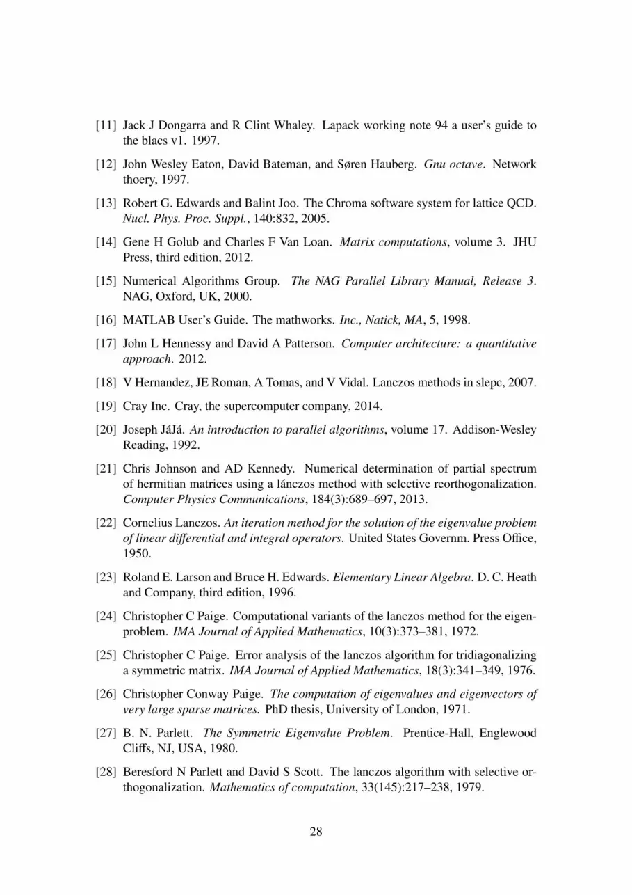
[11] Jack J Dongarra and R Clint Whaley. Lapack working note 94 a user’s guide tothe blacs v1. 1997.

[12] John Wesley Eaton, David Bateman, and Søren Hauberg. Gnu octave. Networkthoery, 1997.

[13] Robert G. Edwards and Balint Joo. The Chroma software system for lattice QCD.Nucl. Phys. Proc. Suppl., 140:832, 2005.

[14] Gene H Golub and Charles F Van Loan. Matrix computations, volume 3. JHUPress, third edition, 2012.

[15] Numerical Algorithms Group. The NAG Parallel Library Manual, Release 3.NAG, Oxford, UK, 2000.

[16] MATLAB User’s Guide. The mathworks. Inc., Natick, MA, 5, 1998.

[17] John L Hennessy and David A Patterson. Computer architecture: a quantitativeapproach. 2012.

[18] V Hernandez, JE Roman, A Tomas, and V Vidal. Lanczos methods in slepc, 2007.

[19] Cray Inc. Cray, the supercomputer company, 2014.

[20] Joseph JáJá. An introduction to parallel algorithms, volume 17. Addison-WesleyReading, 1992.

[21] Chris Johnson and AD Kennedy. Numerical determination of partial spectrumof hermitian matrices using a lánczos method with selective reorthogonalization.Computer Physics Communications, 184(3):689–697, 2013.

[22] Cornelius Lanczos. An iteration method for the solution of the eigenvalue problemof linear differential and integral operators. United States Governm. Press Office,1950.

[23] Roland E. Larson and Bruce H. Edwards. Elementary Linear Algebra. D. C. Heathand Company, third edition, 1996.

[24] Christopher C Paige. Computational variants of the lanczos method for the eigen-problem. IMA Journal of Applied Mathematics, 10(3):373–381, 1972.

[25] Christopher C Paige. Error analysis of the lanczos algorithm for tridiagonalizinga symmetric matrix. IMA Journal of Applied Mathematics, 18(3):341–349, 1976.

[26] Christopher Conway Paige. The computation of eigenvalues and eigenvectors ofvery large sparse matrices. PhD thesis, University of London, 1971.

[27] B. N. Parlett. The Symmetric Eigenvalue Problem. Prentice-Hall, EnglewoodCliffs, NJ, USA, 1980.

[28] Beresford N Parlett and David S Scott. The lanczos algorithm with selective or-thogonalization. Mathematics of computation, 33(145):217–238, 1979.

28

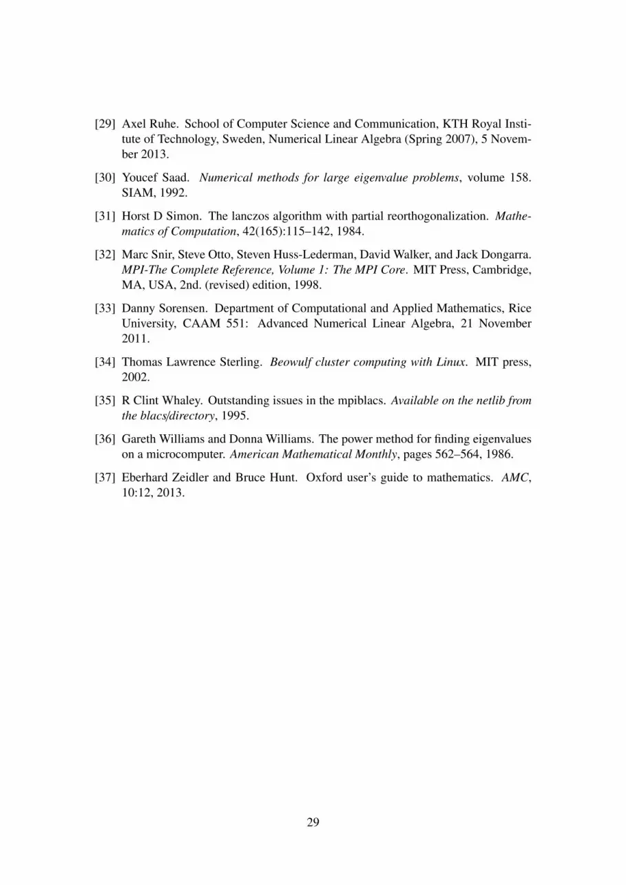
[29] Axel Ruhe. School of Computer Science and Communication, KTH Royal Insti-tute of Technology, Sweden, Numerical Linear Algebra (Spring 2007), 5 Novem-ber 2013.

[30] Youcef Saad. Numerical methods for large eigenvalue problems, volume 158.SIAM, 1992.

[31] Horst D Simon. The lanczos algorithm with partial reorthogonalization. Mathe-matics of Computation, 42(165):115–142, 1984.

[32] Marc Snir, Steve Otto, Steven Huss-Lederman, David Walker, and Jack Dongarra.MPI-The Complete Reference, Volume 1: The MPI Core. MIT Press, Cambridge,MA, USA, 2nd. (revised) edition, 1998.

[33] Danny Sorensen. Department of Computational and Applied Mathematics, RiceUniversity, CAAM 551: Advanced Numerical Linear Algebra, 21 November2011.

[34] Thomas Lawrence Sterling. Beowulf cluster computing with Linux. MIT press,2002.

[35] R Clint Whaley. Outstanding issues in the mpiblacs. Available on the netlib fromthe blacs/directory, 1995.

[36] Gareth Williams and Donna Williams. The power method for finding eigenvalueson a microcomputer. American Mathematical Monthly, pages 562–564, 1986.

[37] Eberhard Zeidler and Bruce Hunt. Oxford user’s guide to mathematics. AMC,10:12, 2013.

29