Introduction to System Identification and Adaptive Controlsaba.kntu.ac.ir/eecd/khakisedigh/Courses/AdvancedControl/index... · 1 Introduction to System Identification and Adaptive

1

Introduction to System Identification and Adaptive Control

A. Khaki SedighControl Systems GroupFaculty of Electrical and Computer EngineeringK. N. Toosi University of TechnologyMay 2009

• Introduction to Adaptive Control

Control System Design Aims to Achieve:

1- Closed Loop Stability 2- Desired Closed Loop Performance (Both

Transient and Steady State)

2

• Some Facts

Real Industrial Plants are Complex in Nature Perfect Modeling Not FeasibleVariations of System Parameters with TimeModel Structure Deficiency: UncertaintyDisturbances and Unknown Noises

• The Feedback Problem

Control systems are designed to maintain closed loop stability with desired closed loop performance in the presence of:

Model UncertaintyTime Varying ParametersDisturbances & Unknown Noises

3

• The Control Engineer Solution Packages:

Robust Control LTI Structure Limited Performance, Strong Mathematical Foundation

Adaptive Control NLTV Structure Nearly Unlimited Performance

Mathematical Foundation Intelligent Control NLTV Structure

Soft computing Mathematical Foundation

• Definition:

To Adapt

- Behavioral Change in order to adjust to new conditions

Adaptive Controller - A controller capable of readjusting its functioning for response

to changes in system dynamics or disturbance input

4

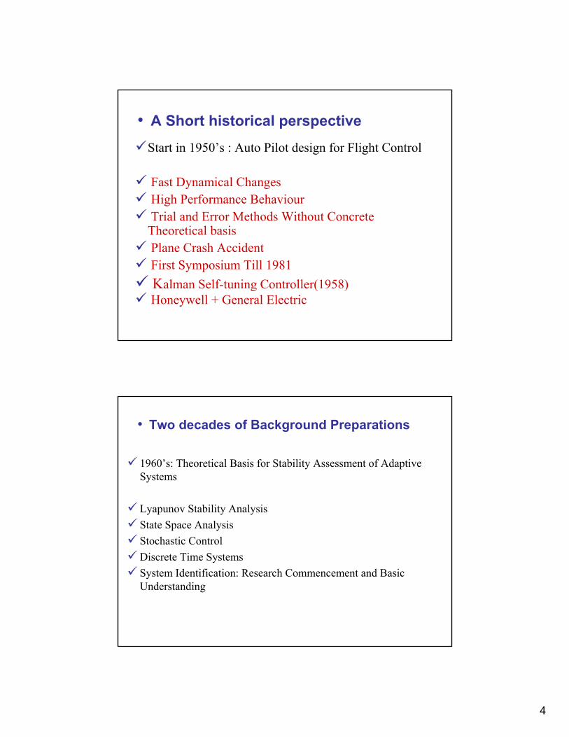
• A Short historical perspective Start in 1950’s : Auto Pilot design for Flight Control

Fast Dynamical ChangesHigh Performance BehaviourTrial and Error Methods Without Concrete Theoretical basisPlane Crash AccidentFirst Symposium Till 1981Kalman Self-tuning Controller(1958)Honeywell + General Electric

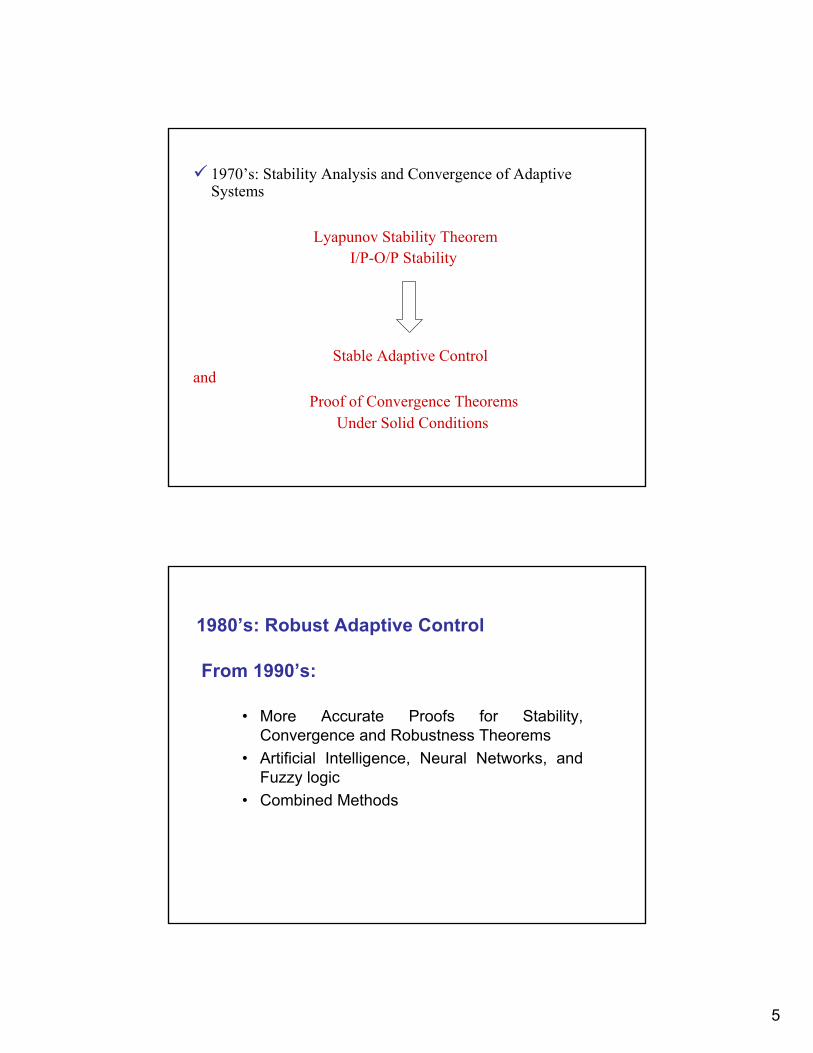
• Two decades of Background Preparations

1960’s: Theoretical Basis for Stability Assessment of Adaptive Systems

Lyapunov Stability AnalysisState Space AnalysisStochastic ControlDiscrete Time SystemsSystem Identification: Research Commencement and Basic Understanding

5

1970’s: Stability Analysis and Convergence of Adaptive Systems

Lyapunov Stability Theorem

I/P-O/P Stability

Stable Adaptive Control

andProof of Convergence Theorems

Under Solid Conditions

1980’s: Robust Adaptive Control

From 1990’s:

• More Accurate Proofs for Stability, Convergence and Robustness Theorems

• Artificial Intelligence, Neural Networks, and Fuzzy logic

• Combined Methods

6

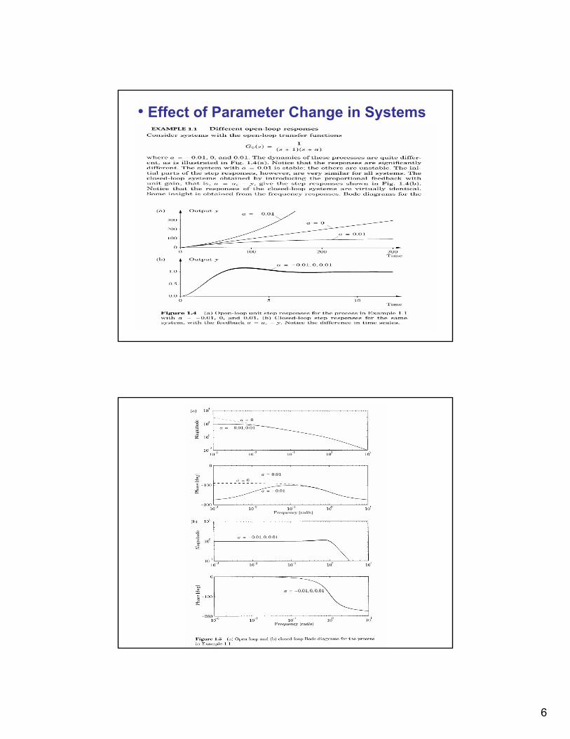
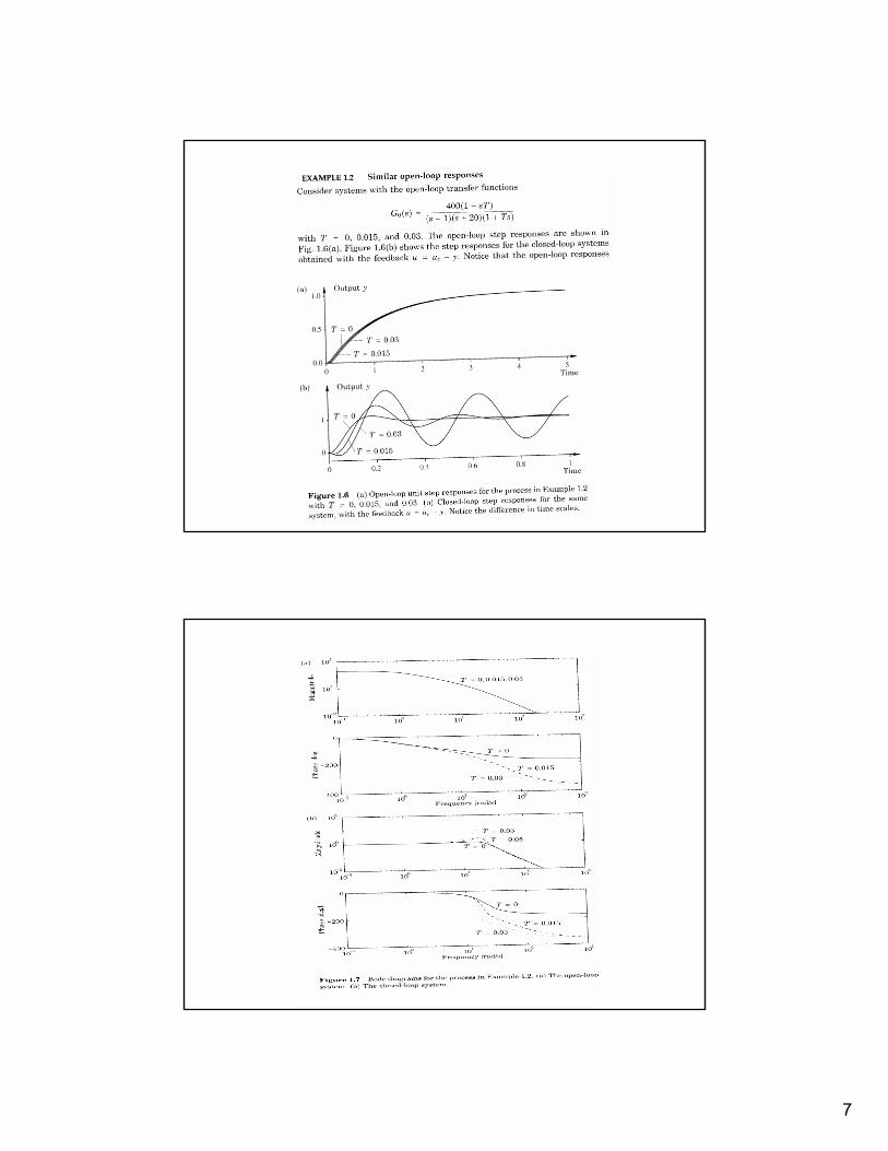
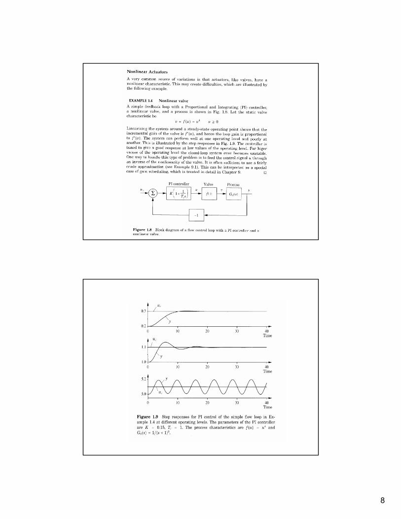
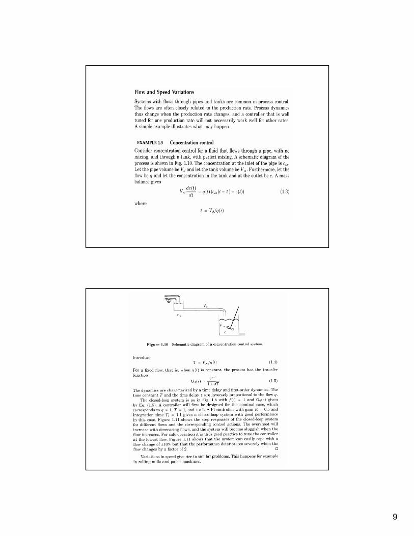
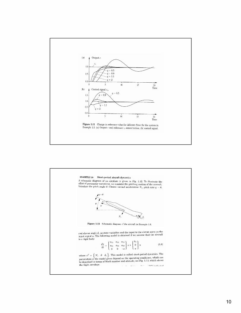
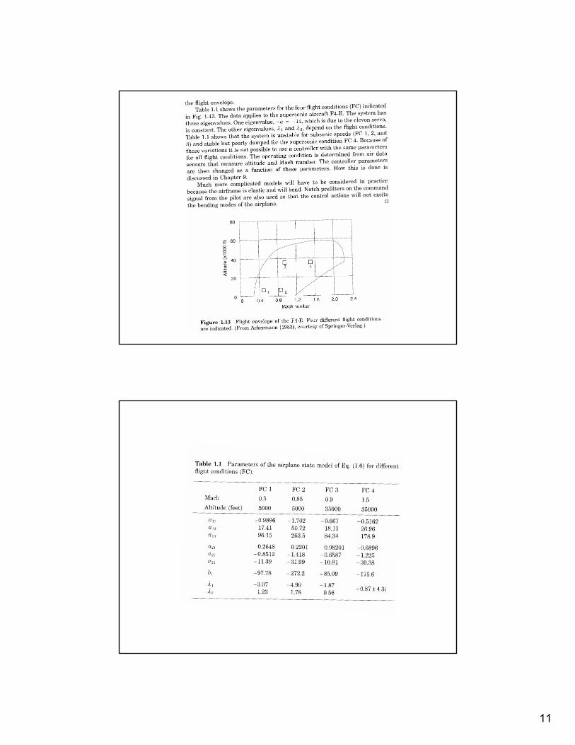
• Effect of Parameter Change in Systems

7

8

9

10

11

12

• PSS• Robots• Level Control• Pressure Control • Flow Control• Temperature Control• PH Control

Some Applications of Adaptive Control

• Main Resolutions of Classical Adaptive Control

Gain SchedulingModel Reference Adaptive System (MRAS)Self tuning Regulators (STR) Self Tuning PIDSelf Oscillating Adaptive Systems (SOAS)

13

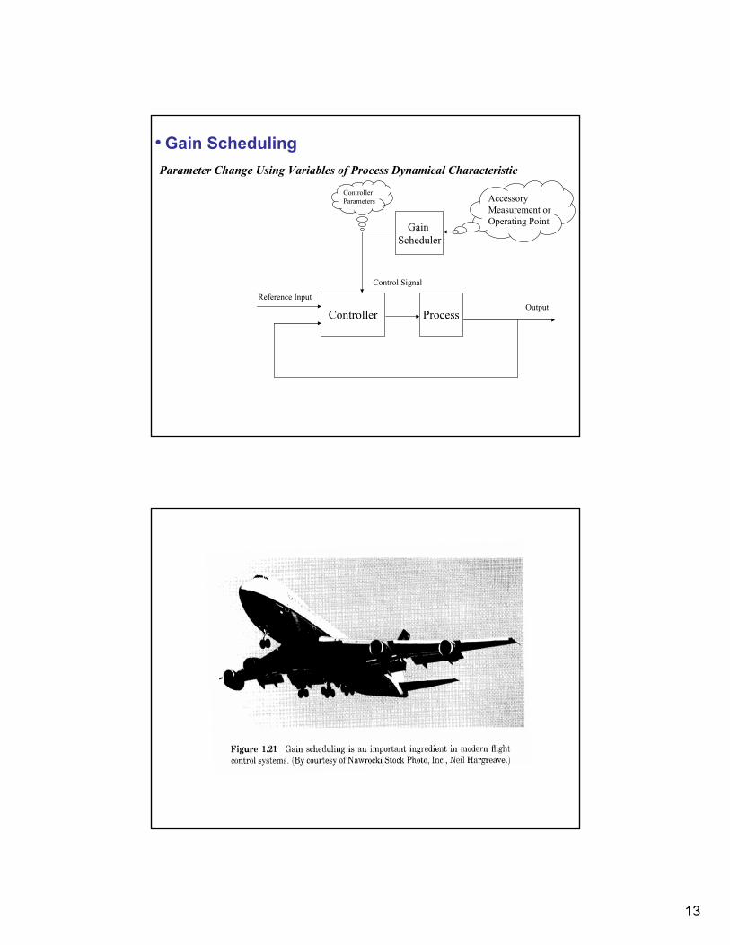
• Gain Scheduling Parameter Change Using Variables of Process Dynamical Characteristic

Gain Scheduler

Controller Process

Accessory Measurement or Operating Point

Controller Parameters

Control Signal

OutputReference Input

14

• Main Characteristics of a Gain Scheduling Controller

Flight Control and Autopilot design

Open Loop Compensation (Parameter Changes)

Is Gain Scheduling Controller Adaptive ?

Many Examples of Practical Application In Industry

Rapid Parameters change (Accessory Measurement)

Number of Operating Points?

• PID Auto Tuning

Methods based on Transient Response

Methods based on Relay Feedback

The Closed Loop Ziegler-Nichols Method

15

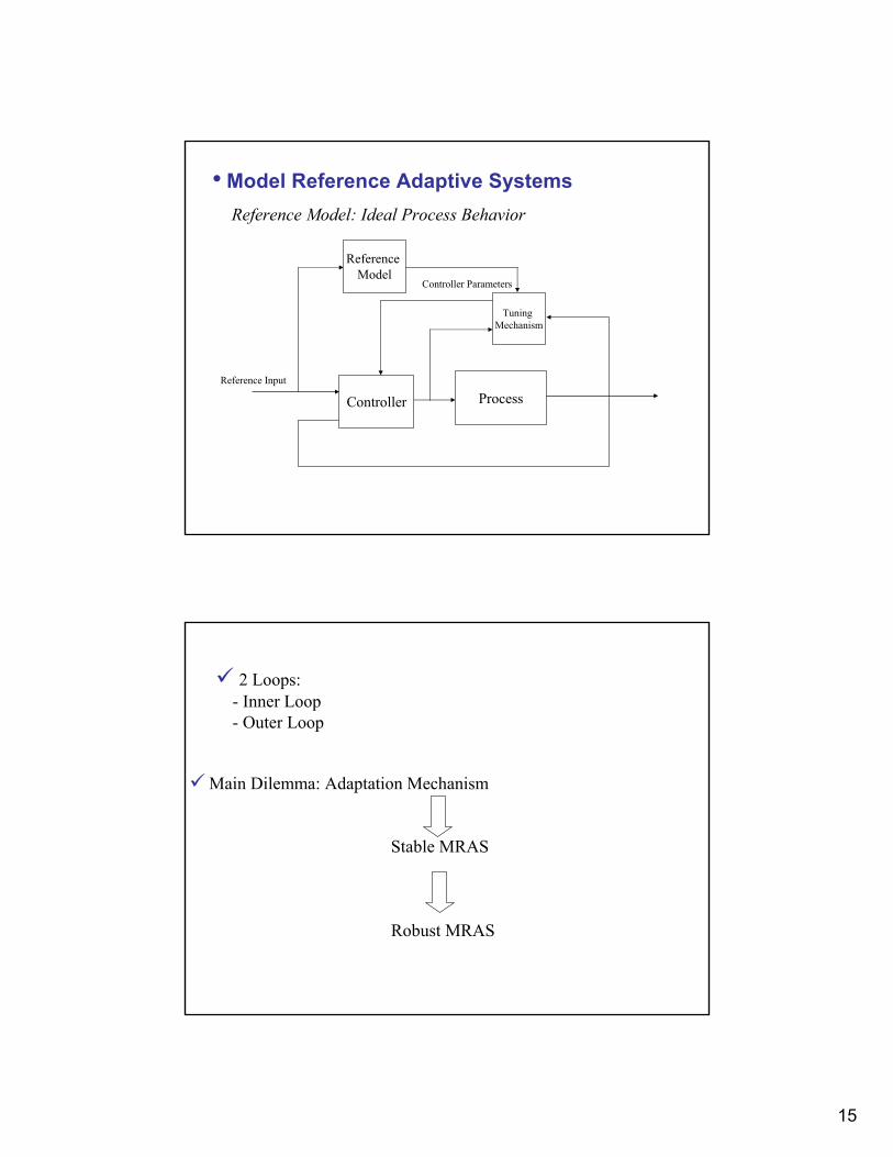
• Model Reference Adaptive Systems Reference Model: Ideal Process Behavior

Controller Process

Tuning Mechanism

Reference Model

Reference Input

Controller Parameters

2 Loops:- Inner Loop- Outer Loop

Main Dilemma: Adaptation Mechanism

Stable MRAS

Robust MRAS

16

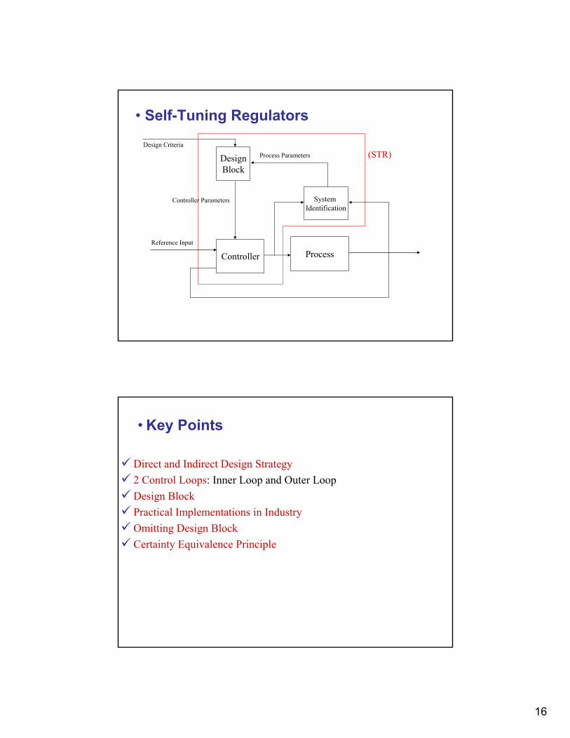
• Self-Tuning Regulators

Controller Process

System Identification

DesignBlock

Reference Input

Design Criteria

Controller Parameters

Process Parameters (STR)

• Key Points

Direct and Indirect Design Strategy 2 Control Loops: Inner Loop and Outer Loop Design BlockPractical Implementations in IndustryOmitting Design BlockCertainty Equivalence Principle

17

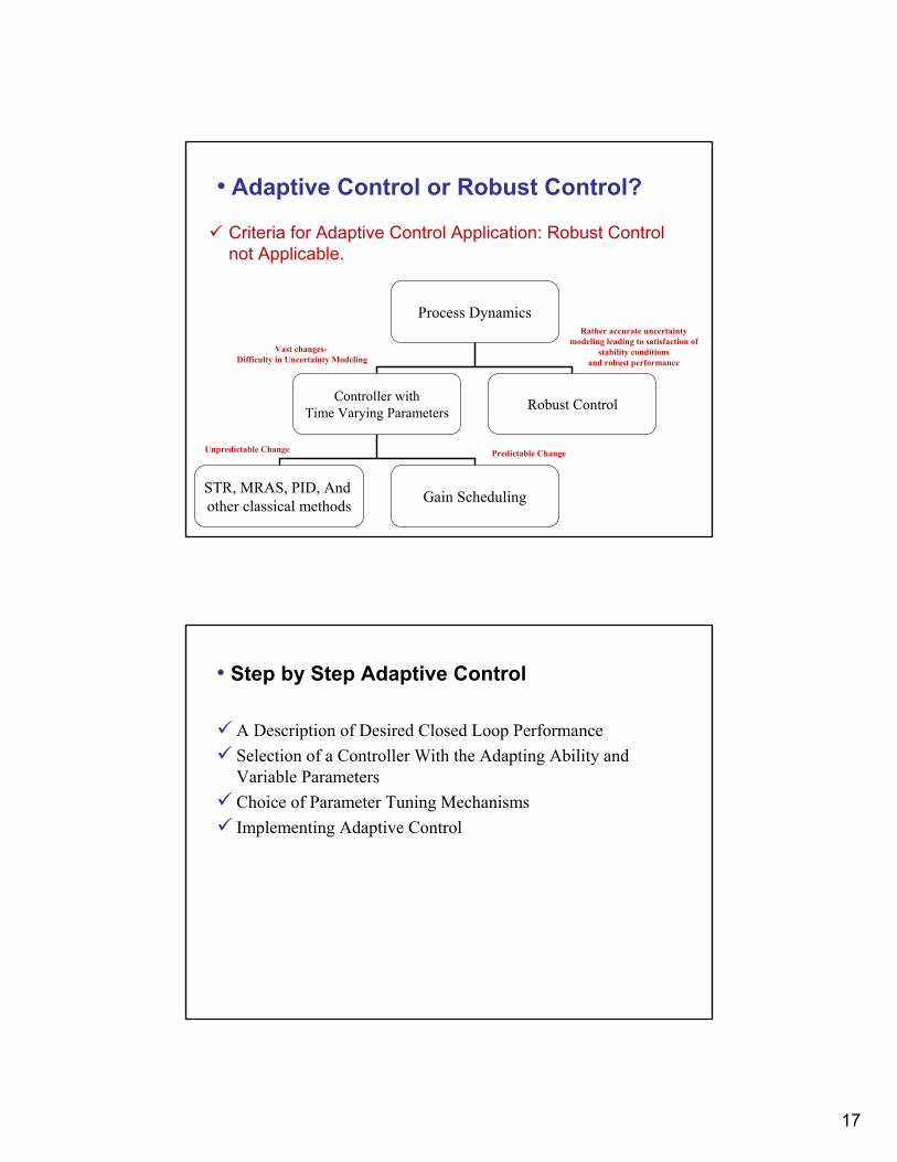
• Adaptive Control or Robust Control?

Criteria for Adaptive Control Application: Robust Control not Applicable.

Process Dynamics

Controller withTime Varying Parameters Robust Control

STR, MRAS, PID, And other classical methods Gain Scheduling

Predictable ChangeUnpredictable Change

Vast changes-Difficulty in Uncertainty Modeling

Rather accurate uncertainty modeling leading to satisfaction of

stability conditions and robust performance

• Step by Step Adaptive Control

A Description of Desired Closed Loop PerformanceSelection of a Controller With the Adapting Ability and Variable ParametersChoice of Parameter Tuning MechanismsImplementing Adaptive Control

18

• Introduction to System Identification

Online Estimation of a Dynamical System’s Parameters is a key element in Adaptive Control.Issues pertaining to system identification

- Model Structure Selection: Linear, Nonlinear, Model Order, Model Type

- Experiment Design: Selection of input for identification- Parameter Estimation: Method for parameter estimation is the

Least Squares Method- Model Validation

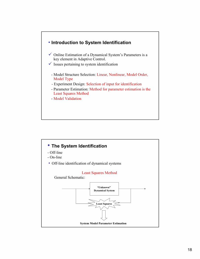
• The System Identification - Off-line- On-line• Off-line identification of dynamical systems

Least Squares MethodGeneral Schematic:

“Unknown”Dynamical System

Least Squares

System Model Parameter Estimation

19

• Least Squares Offline Identification

• Gauss:The sum of squares of the differences between the actually observed (system outputs) and the computed values (model outputs), multiplied by numbers that measure the degree of precision, is Minimum.

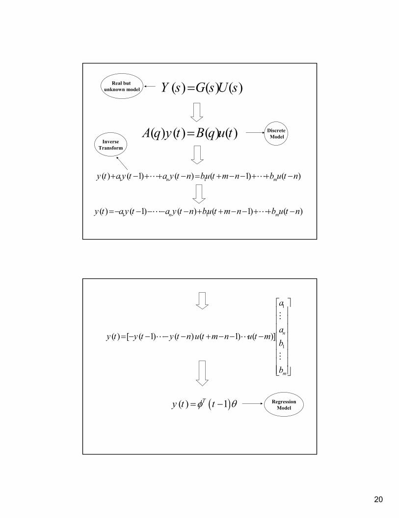
• Describe the unknown plant model in a form that is suitable for system identification methods.

Mathematical Modeling

20

( ) ( ) ( )Y s G s U s=

( ) ( ) ( ) ( )A q y t B q u t=

Real but unknown model

DiscreteModel

1 1( ) ( 1) ( ) ( 1) ( )n my t a y t a y t n bu t m n b u t n+ − + + − = + − − + + −

InverseTransform

1 1( ) ( 1) ( ) ( 1) ( )n my t a y t a y t n bu t m n b u t n=− − − − − + + − − + + −

1

1

( ) [ ( 1) ( ) ( 1) ( )] n

m

a

ay t y t y t n u t m n u t m

b

b

= − − − − + − − −

( )( ) 1Ty t tφ θ= − RegressionModel

21

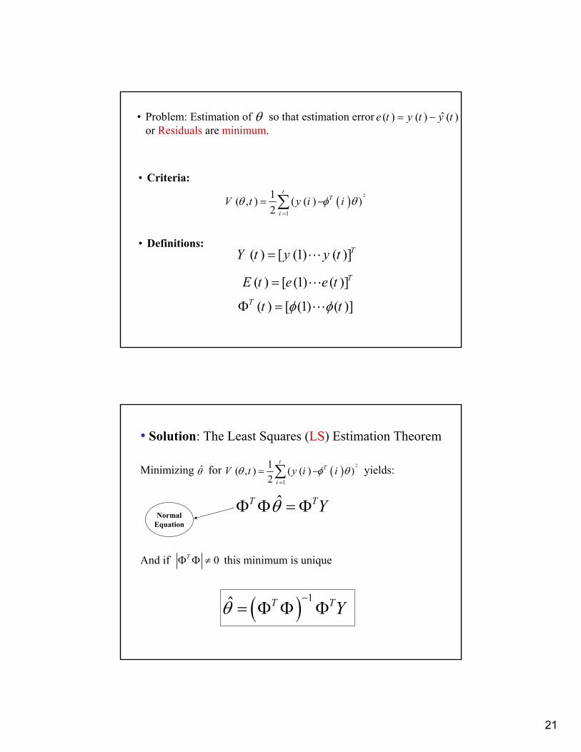
• Problem: Estimation of so that estimation error or Residuals are minimum.

• Criteria:

• Definitions:

( ) 2

1

1( , ) ( ( ) )2

tT

iV t y i iθ φ θ

=

= −∑

θ ˆ( ) ( ) ( )e t y t y t= −

( ) [ (1) ( )]TY t y y t=

( ) [ (1) ( )]TE t e e t=

( ) [ (1) ( )]T t tφ φΦ =

Minimizing for yields:

And if this minimum is unique

• Solution: The Least Squares (LS) Estimation Theorem

θ ( ) 2

1

1( , ) ( ( ) )2

tT

iV t y i iθ φ θ

=

= −∑

ˆT TYθΦ Φ = Φ

0TΦ Φ ≠

( ) 1ˆ T TYθ−

= Φ Φ Φ

NormalEquation

22

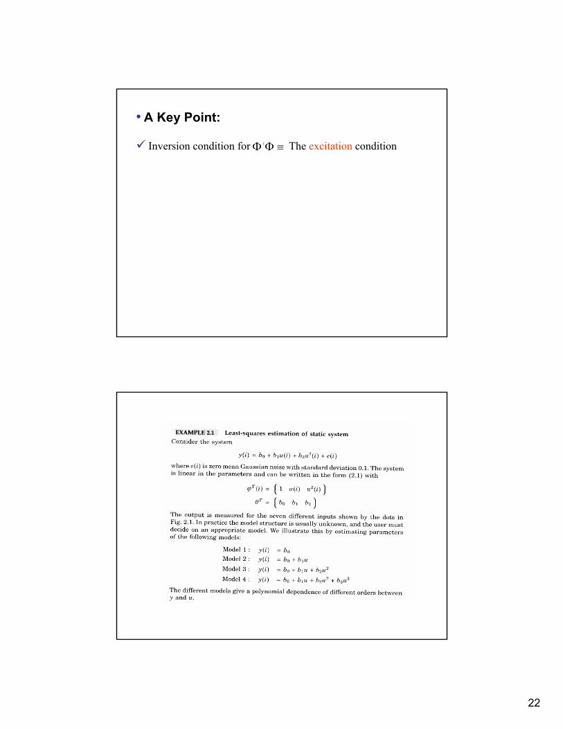
• A Key Point:

Inversion condition for The excitation condition ≡ΦΦ T

23

24

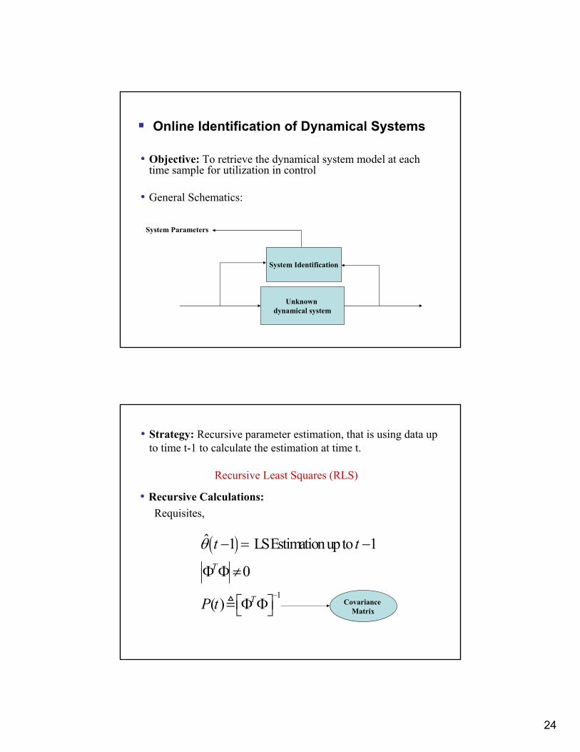
Online Identification of Dynamical Systems

• Objective: To retrieve the dynamical system model at each time sample for utilization in control

• General Schematics:

Unknown dynamical system

System Identification

System Parameters

• Strategy: Recursive parameter estimation, that is using data up to time t-1 to calculate the estimation at time t.

Recursive Least Squares (RLS)

• Recursive Calculations: Requisites,

( )

1

ˆ 1 LS Estimation up to 1

0

( )

T

T

t t

P t

θ

−

− = −

Φ Φ≠

Φ Φ Covariance

Matrix

25

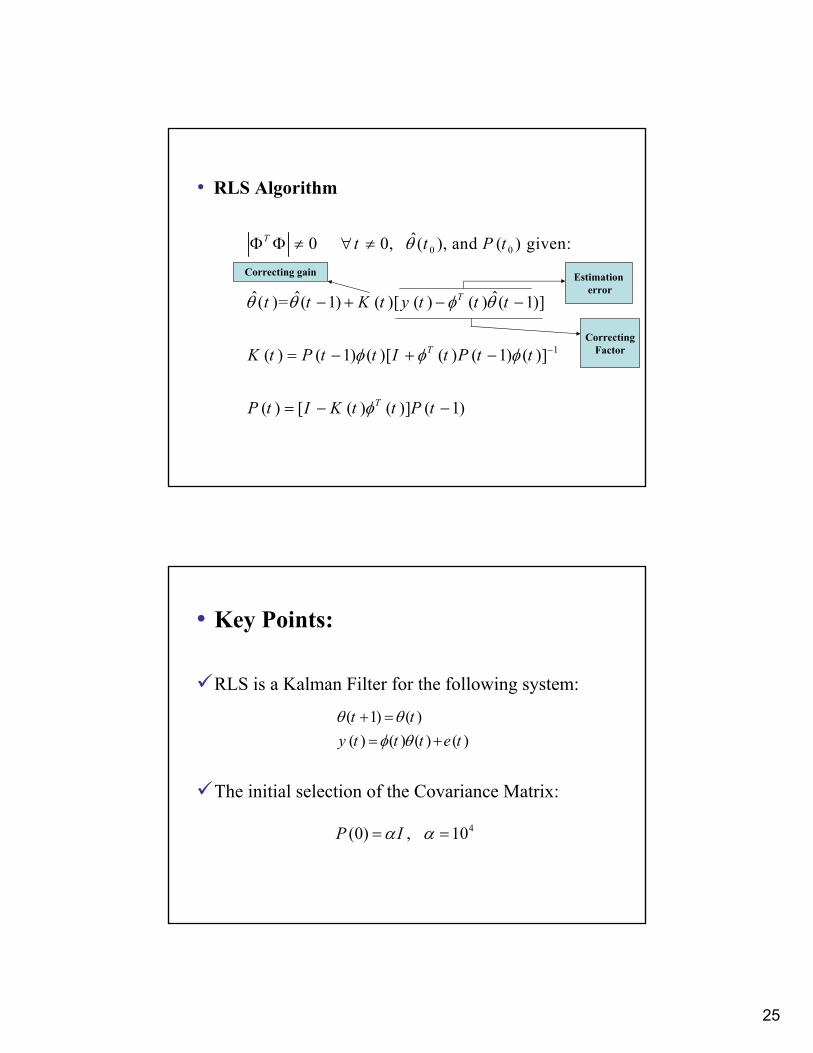
• RLS Algorithm

0 0

1

ˆ0 0, ( ), and ( ) given:

ˆ ˆ ˆ( )= ( 1) ( )[ ( ) ( ) ( 1)]

( ) ( 1) ( )[ ( ) ( 1) ( )]

( ) [ ( ) ( )] ( 1)

T

T

T

T

t t P t

t t K t y t t t

K t P t t I t P t t

P t I K t t P t

θ

θ θ φ θ

φ φ φ

φ

−

Φ Φ ≠ ∀ ≠

− + − −

= − + −

= − −

Correcting gain Estimationerror

CorrectingFactor

• Key Points:

RLS is a Kalman Filter for the following system:

The initial selection of the Covariance Matrix:

( 1) ( )( ) ( ) ( ) ( )t t

y t t t e tθ θ

φ θ+ == +

4(0) , 10P Iα α= =

26

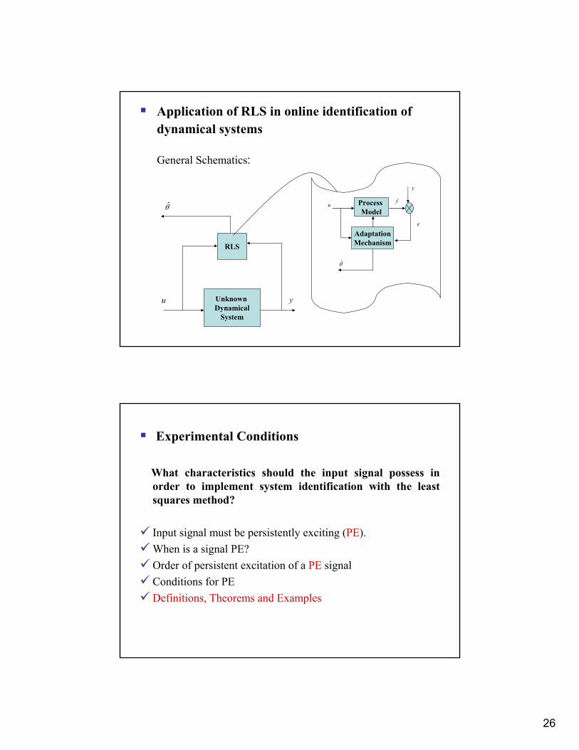
Application of RLS in online identification of dynamical systems

General Schematics:

θ

u

u Unknown Dynamical

System

RLS

Process Model

AdaptationMechanism

u

θ

y

y

y

e

Experimental Conditions

What characteristics should the input signal possess in order to implement system identification with the least squares method?

Input signal must be persistently exciting (PE).When is a signal PE?Order of persistent excitation of a PE signalConditions for PEDefinitions, Theorems and Examples