Introduction to POV-Ray POV-Team for POV-Ray Version 3.6.1

Welcome message from author
This document is posted to help you gain knowledge. Please leave a comment to let me know what you think about it! Share it to your friends and learn new things together.
Transcript
Introduction to POV-Ray
POV-Team
for POV-Ray Version 3.6.1

ii
Contents
1 Introduction 11.1 Program Description . . . . . . . . . . . . . . . . . . . . . . . . . . . . . . . . . . . . . 21.2 What is Ray-Tracing? . . . . . . . . . . . . . . . . . . . . . . . . . . . . . . . . . . . . . 21.3 What is POV-Ray? . . . . . . . . . . . . . . . . . . . . . . . . . . . . . . . . . . . . . . 21.4 Features . . . . . . . . . . . . . . . . . . . . . . . . . . . . . . . . . . . . . . . . . . . . 31.5 The Early History of POV-Ray . . . . . . . . . . . . . . . . . . . . . . . . . . . . . . . . 3
1.5.1 The Original Creation Message . . . . . . . . . . . . . . . . . . . . . . . . . . . 51.5.2 The Name . . . . . . . . . . . . . . . . . . . . . . . . . . . . . . . . . . . . . . . 61.5.3 A Historic ’Version History’ . . . . . . . . . . . . . . . . . . . . . . . . . . . . . 7
1.6 How Do I Begin? . . . . . . . . . . . . . . . . . . . . . . . . . . . . . . . . . . . . . . . 81.7 Notation and Basic Assumptions . . . . . . . . . . . . . . . . . . . . . . . . . . . . . . . 9
2 Getting Started 112.1 Our First Image . . . . . . . . . . . . . . . . . . . . . . . . . . . . . . . . . . . . . . . . 11
2.1.1 Understanding POV-Ray’s Coordinate System . . . . . . . . . . . . . . . . . . . . 112.1.2 Adding Standard Include Files . . . . . . . . . . . . . . . . . . . . . . . . . . . . 122.1.3 Adding a Camera . . . . . . . . . . . . . . . . . . . . . . . . . . . . . . . . . . . 132.1.4 Describing an Object . . . . . . . . . . . . . . . . . . . . . . . . . . . . . . . . . 132.1.5 Adding Texture to an Object . . . . . . . . . . . . . . . . . . . . . . . . . . . . . 142.1.6 Defining a Light Source . . . . . . . . . . . . . . . . . . . . . . . . . . . . . . . 14
2.2 Basic Shapes . . . . . . . . . . . . . . . . . . . . . . . . . . . . . . . . . . . . . . . . . 152.2.1 Box Object . . . . . . . . . . . . . . . . . . . . . . . . . . . . . . . . . . . . . . 152.2.2 Cone Object . . . . . . . . . . . . . . . . . . . . . . . . . . . . . . . . . . . . . 162.2.3 Cylinder Object . . . . . . . . . . . . . . . . . . . . . . . . . . . . . . . . . . . . 162.2.4 Plane Object . . . . . . . . . . . . . . . . . . . . . . . . . . . . . . . . . . . . . 162.2.5 Torus Object . . . . . . . . . . . . . . . . . . . . . . . . . . . . . . . . . . . . . 17
2.3 CSG Objects . . . . . . . . . . . . . . . . . . . . . . . . . . . . . . . . . . . . . . . . . 222.3.1 What is CSG? . . . . . . . . . . . . . . . . . . . . . . . . . . . . . . . . . . . . . 222.3.2 CSG Union . . . . . . . . . . . . . . . . . . . . . . . . . . . . . . . . . . . . . . 222.3.3 CSG Intersection . . . . . . . . . . . . . . . . . . . . . . . . . . . . . . . . . . . 232.3.4 CSG Difference . . . . . . . . . . . . . . . . . . . . . . . . . . . . . . . . . . . . 242.3.5 CSG Merge . . . . . . . . . . . . . . . . . . . . . . . . . . . . . . . . . . . . . . 252.3.6 CSG Pitfalls . . . . . . . . . . . . . . . . . . . . . . . . . . . . . . . . . . . . . 26
2.4 The Light Source . . . . . . . . . . . . . . . . . . . . . . . . . . . . . . . . . . . . . . . 262.4.1 The Pointlight Source . . . . . . . . . . . . . . . . . . . . . . . . . . . . . . . . 262.4.2 The Spotlight Source . . . . . . . . . . . . . . . . . . . . . . . . . . . . . . . . . 282.4.3 The Cylindrical Light Source . . . . . . . . . . . . . . . . . . . . . . . . . . . . . 292.4.4 The Area Light Source . . . . . . . . . . . . . . . . . . . . . . . . . . . . . . . . 292.4.5 The Ambient Light Source . . . . . . . . . . . . . . . . . . . . . . . . . . . . . . 302.4.6 Light Source Specials . . . . . . . . . . . . . . . . . . . . . . . . . . . . . . . . 31
2.5 Simple Texture Options . . . . . . . . . . . . . . . . . . . . . . . . . . . . . . . . . . . . 33
iv CONTENTS
2.5.1 Surface Finishes . . . . . . . . . . . . . . . . . . . . . . . . . . . . . . . . . . . 332.5.2 Adding Bumpiness . . . . . . . . . . . . . . . . . . . . . . . . . . . . . . . . . . 332.5.3 Creating Color Patterns . . . . . . . . . . . . . . . . . . . . . . . . . . . . . . . . 332.5.4 Pre-defined Textures . . . . . . . . . . . . . . . . . . . . . . . . . . . . . . . . . 34
2.6 Using the Camera . . . . . . . . . . . . . . . . . . . . . . . . . . . . . . . . . . . . . . . 352.6.1 Using Focal Blur . . . . . . . . . . . . . . . . . . . . . . . . . . . . . . . . . . . 35
2.7 POV-Ray Coordinate System . . . . . . . . . . . . . . . . . . . . . . . . . . . . . . . . . 372.7.1 Transformations . . . . . . . . . . . . . . . . . . . . . . . . . . . . . . . . . . . 372.7.2 Transformation Order . . . . . . . . . . . . . . . . . . . . . . . . . . . . . . . . 392.7.3 Inverse Transform . . . . . . . . . . . . . . . . . . . . . . . . . . . . . . . . . . 392.7.4 Transform Identifiers . . . . . . . . . . . . . . . . . . . . . . . . . . . . . . . . . 402.7.5 Transforming Textures and Objects . . . . . . . . . . . . . . . . . . . . . . . . . 40
2.8 Setting POV-Ray Options . . . . . . . . . . . . . . . . . . . . . . . . . . . . . . . . . . . 412.8.1 Command Line Switches . . . . . . . . . . . . . . . . . . . . . . . . . . . . . . . 412.8.2 Using INI Files . . . . . . . . . . . . . . . . . . . . . . . . . . . . . . . . . . . . 422.8.3 Using the POVINI Environment Variable . . . . . . . . . . . . . . . . . . . . . . 43
3 Advanced Features 453.1 Spline Based Shapes . . . . . . . . . . . . . . . . . . . . . . . . . . . . . . . . . . . . . 45
3.1.1 Lathe Object . . . . . . . . . . . . . . . . . . . . . . . . . . . . . . . . . . . . . 453.1.2 Surface of Revolution Object . . . . . . . . . . . . . . . . . . . . . . . . . . . . . 523.1.3 Prism Object . . . . . . . . . . . . . . . . . . . . . . . . . . . . . . . . . . . . . 543.1.4 Sphere Sweep Object . . . . . . . . . . . . . . . . . . . . . . . . . . . . . . . . . 593.1.5 Bicubic Patch Object . . . . . . . . . . . . . . . . . . . . . . . . . . . . . . . . . 603.1.6 Text Object . . . . . . . . . . . . . . . . . . . . . . . . . . . . . . . . . . . . . . 65
3.2 Polygon Based Shapes . . . . . . . . . . . . . . . . . . . . . . . . . . . . . . . . . . . . 673.2.1 Mesh Object . . . . . . . . . . . . . . . . . . . . . . . . . . . . . . . . . . . . . 673.2.2 Mesh2 Object . . . . . . . . . . . . . . . . . . . . . . . . . . . . . . . . . . . . . 693.2.3 Polygon Object . . . . . . . . . . . . . . . . . . . . . . . . . . . . . . . . . . . . 75
3.3 Other Shapes . . . . . . . . . . . . . . . . . . . . . . . . . . . . . . . . . . . . . . . . . 773.3.1 Blob Object . . . . . . . . . . . . . . . . . . . . . . . . . . . . . . . . . . . . . . 773.3.2 Height Field Object . . . . . . . . . . . . . . . . . . . . . . . . . . . . . . . . . . 813.3.3 Isosurface Object . . . . . . . . . . . . . . . . . . . . . . . . . . . . . . . . . . . 833.3.4 Poly Object . . . . . . . . . . . . . . . . . . . . . . . . . . . . . . . . . . . . . . 973.3.5 Superquadric Ellipsoid Object . . . . . . . . . . . . . . . . . . . . . . . . . . . . 103
3.4 Advanced Texture Options . . . . . . . . . . . . . . . . . . . . . . . . . . . . . . . . . . 1063.4.1 Pigments . . . . . . . . . . . . . . . . . . . . . . . . . . . . . . . . . . . . . . . 1063.4.2 Normals . . . . . . . . . . . . . . . . . . . . . . . . . . . . . . . . . . . . . . . . 1113.4.3 Finishes . . . . . . . . . . . . . . . . . . . . . . . . . . . . . . . . . . . . . . . . 1133.4.4 Working With Pigment Maps . . . . . . . . . . . . . . . . . . . . . . . . . . . . . 1183.4.5 Working With Normal Maps . . . . . . . . . . . . . . . . . . . . . . . . . . . . . 1193.4.6 Working With Texture Maps . . . . . . . . . . . . . . . . . . . . . . . . . . . . . 1193.4.7 Working With List Textures . . . . . . . . . . . . . . . . . . . . . . . . . . . . . 1203.4.8 What About Tiles? . . . . . . . . . . . . . . . . . . . . . . . . . . . . . . . . . . 1213.4.9 Average Function . . . . . . . . . . . . . . . . . . . . . . . . . . . . . . . . . . . 1213.4.10 Working With Layered Textures . . . . . . . . . . . . . . . . . . . . . . . . . . . 1223.4.11 When All Else Fails: Material Maps . . . . . . . . . . . . . . . . . . . . . . . . . 1273.4.12 Limitations Of Special Textures . . . . . . . . . . . . . . . . . . . . . . . . . . . 129
3.5 Using Atmospheric Effects . . . . . . . . . . . . . . . . . . . . . . . . . . . . . . . . . . 1303.5.1 The Background . . . . . . . . . . . . . . . . . . . . . . . . . . . . . . . . . . . 1303.5.2 The Sky Sphere . . . . . . . . . . . . . . . . . . . . . . . . . . . . . . . . . . . . 1313.5.3 The Fog . . . . . . . . . . . . . . . . . . . . . . . . . . . . . . . . . . . . . . . . 1343.5.4 The Rainbow . . . . . . . . . . . . . . . . . . . . . . . . . . . . . . . . . . . . . 139
CONTENTS v
3.6 Simple Media Tutorial . . . . . . . . . . . . . . . . . . . . . . . . . . . . . . . . . . . . 1433.6.1 Types of media . . . . . . . . . . . . . . . . . . . . . . . . . . . . . . . . . . . . 1433.6.2 Some media concepts . . . . . . . . . . . . . . . . . . . . . . . . . . . . . . . . . 1433.6.3 Simple media examples . . . . . . . . . . . . . . . . . . . . . . . . . . . . . . . 1443.6.4 Multiple medias inside the same object . . . . . . . . . . . . . . . . . . . . . . . 1473.6.5 Media and transformations . . . . . . . . . . . . . . . . . . . . . . . . . . . . . . 1483.6.6 A more advanced example of scattering media . . . . . . . . . . . . . . . . . . . 1493.6.7 Media and photons . . . . . . . . . . . . . . . . . . . . . . . . . . . . . . . . . . 149
3.7 Radiosity . . . . . . . . . . . . . . . . . . . . . . . . . . . . . . . . . . . . . . . . . . . 1503.7.1 Introduction . . . . . . . . . . . . . . . . . . . . . . . . . . . . . . . . . . . . . . 1503.7.2 Radiosity with conventional lighting . . . . . . . . . . . . . . . . . . . . . . . . . 1513.7.3 Radiosity without conventional lighting . . . . . . . . . . . . . . . . . . . . . . . 1553.7.4 Normals and Radiosity . . . . . . . . . . . . . . . . . . . . . . . . . . . . . . . . 1593.7.5 Performance considerations . . . . . . . . . . . . . . . . . . . . . . . . . . . . . 159
3.8 Making Animations . . . . . . . . . . . . . . . . . . . . . . . . . . . . . . . . . . . . . . 1603.8.1 The Clock Variable: Key To It All . . . . . . . . . . . . . . . . . . . . . . . . . . 1603.8.2 Clock Dependant Variables And Multi-Stage Animations . . . . . . . . . . . . . . 1613.8.3 The Phase Keyword . . . . . . . . . . . . . . . . . . . . . . . . . . . . . . . . . 1633.8.4 Do Not Use Jitter Or Crand . . . . . . . . . . . . . . . . . . . . . . . . . . . . . 1643.8.5 INI File Settings . . . . . . . . . . . . . . . . . . . . . . . . . . . . . . . . . . . 164
3.9 While-loop tutorial . . . . . . . . . . . . . . . . . . . . . . . . . . . . . . . . . . . . . . 1653.9.1 What a while-loop is and what it is not . . . . . . . . . . . . . . . . . . . . . . . . 1653.9.2 How does a single while-loop work? . . . . . . . . . . . . . . . . . . . . . . . . . 1663.9.3 How do I make a while-loop? . . . . . . . . . . . . . . . . . . . . . . . . . . . . 1663.9.4 What is a condition and how do I make one? . . . . . . . . . . . . . . . . . . . . 1673.9.5 What about loop types other than simple for-loops? . . . . . . . . . . . . . . . . . 1683.9.6 What about nested loops? . . . . . . . . . . . . . . . . . . . . . . . . . . . . . . 1693.9.7 Mixed-type nested loops . . . . . . . . . . . . . . . . . . . . . . . . . . . . . . . 1713.9.8 Other things to note . . . . . . . . . . . . . . . . . . . . . . . . . . . . . . . . . . 171
3.10 SDL tutorial: A raytracer . . . . . . . . . . . . . . . . . . . . . . . . . . . . . . . . . . . 1733.10.1 Introduction . . . . . . . . . . . . . . . . . . . . . . . . . . . . . . . . . . . . . . 1733.10.2 The idea and the code . . . . . . . . . . . . . . . . . . . . . . . . . . . . . . . . 1743.10.3 Short introduction to raytracing . . . . . . . . . . . . . . . . . . . . . . . . . . . 1783.10.4 Global settings . . . . . . . . . . . . . . . . . . . . . . . . . . . . . . . . . . . . 1793.10.5 Scene definition . . . . . . . . . . . . . . . . . . . . . . . . . . . . . . . . . . . . 1803.10.6 Initializing the raytracer . . . . . . . . . . . . . . . . . . . . . . . . . . . . . . . 1813.10.7 Ray-sphere intersection . . . . . . . . . . . . . . . . . . . . . . . . . . . . . . . . 1813.10.8 The Trace macro . . . . . . . . . . . . . . . . . . . . . . . . . . . . . . . . . . . 1853.10.9 Calculating the image . . . . . . . . . . . . . . . . . . . . . . . . . . . . . . . . 1893.10.10 Creating the colored mesh . . . . . . . . . . . . . . . . . . . . . . . . . . . . . . 1903.10.11 The Camera-setup . . . . . . . . . . . . . . . . . . . . . . . . . . . . . . . . . . 194
4 Questions and Tips 1954.1 Language Tips and tricks to achieve useful things . . . . . . . . . . . . . . . . . . . . . . 195
4.1.1 How do I make a visible light source? . . . . . . . . . . . . . . . . . . . . . . . . 1954.1.2 How do I make bright objects? . . . . . . . . . . . . . . . . . . . . . . . . . . . . 1964.1.3 How do I move the camera in a circular path? . . . . . . . . . . . . . . . . . . . . 1964.1.4 How do I use an image to texture my object? . . . . . . . . . . . . . . . . . . . . 1974.1.5 How can I generate a spline? . . . . . . . . . . . . . . . . . . . . . . . . . . . . . 1974.1.6 How can I simulate motion blur? . . . . . . . . . . . . . . . . . . . . . . . . . . . 1974.1.7 How can I find the size of a text object? . . . . . . . . . . . . . . . . . . . . . . . 1984.1.8 How do I make extruded text? . . . . . . . . . . . . . . . . . . . . . . . . . . . . 1984.1.9 How do I make an object hollow? . . . . . . . . . . . . . . . . . . . . . . . . . . 198
vi CONTENTS
4.1.10 How can I fill a glass with water or other objects? . . . . . . . . . . . . . . . . . . 1994.1.11 How can I bend a object? . . . . . . . . . . . . . . . . . . . . . . . . . . . . . . . 2004.1.12 Can I get non-grainy focal blur? . . . . . . . . . . . . . . . . . . . . . . . . . . . 200
4.2 Language Things that don’t work as one expects . . . . . . . . . . . . . . . . . . . . . . . 2004.2.1 Using several transparent objects makes them black? . . . . . . . . . . . . . . . . 2004.2.2 I’m getting color banding in the image . . . . . . . . . . . . . . . . . . . . . . . . 2014.2.3 Rotation behaves very strangely . . . . . . . . . . . . . . . . . . . . . . . . . . . 2014.2.4 The image gets distorted when rendering a square image . . . . . . . . . . . . . . 2024.2.5 Why are there strange dark pixels or noise on my CSG object? . . . . . . . . . . . 2034.2.6 Why won’t the textures in stars.inc work with my skysphere? . . . . . . . . . . . 2034.2.7 When I use filter or transmit with my .tga image map nothing happens. . . . . . . 2044.2.8 Isosurface not rendering properly? . . . . . . . . . . . . . . . . . . . . . . . . . . 204
4.3 Language related things . . . . . . . . . . . . . . . . . . . . . . . . . . . . . . . . . . . . 2044.3.1 How do I turn animation on? . . . . . . . . . . . . . . . . . . . . . . . . . . . . . 2044.3.2 Can POV-Ray use multiple processors? . . . . . . . . . . . . . . . . . . . . . . . 2054.3.3 Can I get a wireframe render of my scene? . . . . . . . . . . . . . . . . . . . . . 2064.3.4 Can I specify variable IOR for an object? . . . . . . . . . . . . . . . . . . . . . . 2074.3.5 What is Photon Mapping? . . . . . . . . . . . . . . . . . . . . . . . . . . . . . . 208
4.4 File Formats . . . . . . . . . . . . . . . . . . . . . . . . . . . . . . . . . . . . . . . . . . 2084.4.1 Saving the image to disk. . . . . . . . . . . . . . . . . . . . . . . . . . . . . . . . 2084.4.2 Can I convert my POV-Ray scenes to another format? . . . . . . . . . . . . . . . . 2094.4.3 How can I convert my scenes from format X to POV-Ray format? . . . . . . . . . 2094.4.4 How do I import all of my textures I created in 3DS Max into POV-Ray? . . . . . 2094.4.5 How can I avoid artifacts and still get good JPEG compression? . . . . . . . . . . 2104.4.6 Why are there no converters from POV to other formats? . . . . . . . . . . . . . . 2104.4.7 Why are triangle meshes in ASCII format? . . . . . . . . . . . . . . . . . . . . . 211
4.5 Utilities, models, etc. . . . . . . . . . . . . . . . . . . . . . . . . . . . . . . . . . . . . . 2124.5.1 What is the best animation program available? . . . . . . . . . . . . . . . . . . . 2124.5.2 Creating/viewing MPEG-files. . . . . . . . . . . . . . . . . . . . . . . . . . . . . 2124.5.3 Where can I find models/textures? . . . . . . . . . . . . . . . . . . . . . . . . . . 2124.5.4 What are the best modellers for POV-Ray? . . . . . . . . . . . . . . . . . . . . . 2124.5.5 Any POV-Ray modellers for Mac? . . . . . . . . . . . . . . . . . . . . . . . . . . 2124.5.6 Is there any user gallery of POV-Ray images? . . . . . . . . . . . . . . . . . . . . 2124.5.7 Any good heightfield modellers? . . . . . . . . . . . . . . . . . . . . . . . . . . . 2134.5.8 Any easy way of creating trees? . . . . . . . . . . . . . . . . . . . . . . . . . . . 213
4.6 Rendering speed . . . . . . . . . . . . . . . . . . . . . . . . . . . . . . . . . . . . . . . . 2134.6.1 Will POV-Ray render faster with a 3D card? . . . . . . . . . . . . . . . . . . . . . 2134.6.2 How do I increase rendering speed? . . . . . . . . . . . . . . . . . . . . . . . . . 2134.6.3 CSG speed . . . . . . . . . . . . . . . . . . . . . . . . . . . . . . . . . . . . . . 2154.6.4 Does POV-Ray support 3DNow? . . . . . . . . . . . . . . . . . . . . . . . . . . . 217
4.7 Miscellaneous questions . . . . . . . . . . . . . . . . . . . . . . . . . . . . . . . . . . . 2174.7.1 Where do I suggest new features? . . . . . . . . . . . . . . . . . . . . . . . . . . 2174.7.2 I’m getting a ”Illegal grid value in ddatraversal()” . . . . . . . . . . . . . . . . . 2184.7.3 No beep when finished? . . . . . . . . . . . . . . . . . . . . . . . . . . . . . . . 2184.7.4 POV-Ray viruses? . . . . . . . . . . . . . . . . . . . . . . . . . . . . . . . . . . 2184.7.5 GUI for Unix POV-Ray? . . . . . . . . . . . . . . . . . . . . . . . . . . . . . . . 218
4.8 The shadow line artifact . . . . . . . . . . . . . . . . . . . . . . . . . . . . . . . . . . . . 2194.8.1 What is the problem? . . . . . . . . . . . . . . . . . . . . . . . . . . . . . . . . . 2194.8.2 What causes the problem? . . . . . . . . . . . . . . . . . . . . . . . . . . . . . . 2204.8.3 Can this problem be solved? . . . . . . . . . . . . . . . . . . . . . . . . . . . . . 2224.8.4 Possible solutions? . . . . . . . . . . . . . . . . . . . . . . . . . . . . . . . . . . 222
4.9 Smooth triangle artifact . . . . . . . . . . . . . . . . . . . . . . . . . . . . . . . . . . . . 2234.9.1 What is the problem? . . . . . . . . . . . . . . . . . . . . . . . . . . . . . . . . . 223
CONTENTS vii
4.9.2 What causes the problem? . . . . . . . . . . . . . . . . . . . . . . . . . . . . . . 2244.9.3 Can this problem be solved? . . . . . . . . . . . . . . . . . . . . . . . . . . . . . 225
5 Appendices 2275.1 POV-Ray User License . . . . . . . . . . . . . . . . . . . . . . . . . . . . . . . . . . . . 2275.2 Citing POV-Ray in Academic Publications . . . . . . . . . . . . . . . . . . . . . . . . . . 2305.3 The POV-Team . . . . . . . . . . . . . . . . . . . . . . . . . . . . . . . . . . . . . . . . 230
5.3.1 Contacting the Authors . . . . . . . . . . . . . . . . . . . . . . . . . . . . . . . . 2355.3.2 The TAG . . . . . . . . . . . . . . . . . . . . . . . . . . . . . . . . . . . . . . . 2355.3.3 POV-Ray 3.6 Development . . . . . . . . . . . . . . . . . . . . . . . . . . . . . . 236
5.4 What to do if you don’t have POV-Ray . . . . . . . . . . . . . . . . . . . . . . . . . . . . 2365.4.1 Which Version of POV-Ray should you use? . . . . . . . . . . . . . . . . . . . . 2365.4.2 Where to Find POV-Ray Files . . . . . . . . . . . . . . . . . . . . . . . . . . . . 239
5.5 Suggested Reading . . . . . . . . . . . . . . . . . . . . . . . . . . . . . . . . . . . . . . 240

viii CONTENTS
Figures
2.1 The left-handed coordinate system . . . . . . . . . . . . . . . . . . . . . . . . . . . . . . 122.2 Computer Graphics Aerobics . . . . . . . . . . . . . . . . . . . . . . . . . . . . . . . . . 122.3 The torus object can be used to create chains. . . . . . . . . . . . . . . . . . . . . . . . . 22
3.1 A simple lathe object. . . . . . . . . . . . . . . . . . . . . . . . . . . . . . . . . . . . . . 463.2 A simple . . . . . . . . . . . . . . . . . . . . . . . . . . . . . . . . . . . . . . . . . . . 483.3 Moving some points of the spline. . . . . . . . . . . . . . . . . . . . . . . . . . . . . . . 493.4 A quadratic spline lathe. . . . . . . . . . . . . . . . . . . . . . . . . . . . . . . . . . . . 493.5 A cubic spline lathe. . . . . . . . . . . . . . . . . . . . . . . . . . . . . . . . . . . . . . 503.6 a bezierspline lathe . . . . . . . . . . . . . . . . . . . . . . . . . . . . . . . . . . . . . . 513.7 two bezierspline segments, not smooth . . . . . . . . . . . . . . . . . . . . . . . . . . . 523.8 smooth bezierspline lathe . . . . . . . . . . . . . . . . . . . . . . . . . . . . . . . . . . 523.9 The point configuration of our cup object. . . . . . . . . . . . . . . . . . . . . . . . . . . 533.10 A surface of revolution object. . . . . . . . . . . . . . . . . . . . . . . . . . . . . . . . . 543.11 A hexagonal prism shape. . . . . . . . . . . . . . . . . . . . . . . . . . . . . . . . . . . . 553.12 A cubic, triangular prism shape. . . . . . . . . . . . . . . . . . . . . . . . . . . . . . . . 563.13 Using sub-shapes to create a more complex shape. . . . . . . . . . . . . . . . . . . . . . . 573.14 Creating a pyramid using conic sweeping. . . . . . . . . . . . . . . . . . . . . . . . . . . 583.15 Choosing a second height larger than one for the conic sweep. . . . . . . . . . . . . . . . 583.16 Increasing the first height for the conic sweep. . . . . . . . . . . . . . . . . . . . . . . . . 593.17 Bicubicpatch with control points . . . . . . . . . . . . . . . . . . . . . . . . . . . . . . . 623.18 patches, (un)smoothly connected . . . . . . . . . . . . . . . . . . . . . . . . . . . . . . . 633.19 3 patches, some control points . . . . . . . . . . . . . . . . . . . . . . . . . . . . . . . . 653.20 Text carved from stone. . . . . . . . . . . . . . . . . . . . . . . . . . . . . . . . . . . . . 683.21 to be written as mesh2 . . . . . . . . . . . . . . . . . . . . . . . . . . . . . . . . . . . . 703.22 The word . . . . . . . . . . . . . . . . . . . . . . . . . . . . . . . . . . . . . . . . . . . 773.23 A simple, two-part blob. . . . . . . . . . . . . . . . . . . . . . . . . . . . . . . . . . . . 783.24 The spherical components made visible. . . . . . . . . . . . . . . . . . . . . . . . . . . . 783.25 A hand made with blobs. . . . . . . . . . . . . . . . . . . . . . . . . . . . . . . . . . . . 803.26 The hand without the swollen joints. . . . . . . . . . . . . . . . . . . . . . . . . . . . . . 813.27 A height field created completely with POV-Ray. . . . . . . . . . . . . . . . . . . . . . . 833.28 Isosurface sample (function{ x }) . . . . . . . . . . . . . . . . . . . . . . . . . . . . . . 843.29 Isosurface sample (function{ x }, threshold 1) . . . . . . . . . . . . . . . . . . . . . . . . 843.30 Isosurface sample (function{ x }, open) . . . . . . . . . . . . . . . . . . . . . . . . . . . 843.31 Isosurface sample (plane function) . . . . . . . . . . . . . . . . . . . . . . . . . . . . . . 853.32 Isosurface sample (plane function) . . . . . . . . . . . . . . . . . . . . . . . . . . . . . . 853.33 Isosurface sample (function{ abs(x)-1}, open) . . . . . . . . . . . . . . . . . . . . . . . 863.34 Isosurface sample (combined linear functions) . . . . . . . . . . . . . . . . . . . . . . . . 863.35 Isosurface sample (combined linear functions) . . . . . . . . . . . . . . . . . . . . . . . . 863.36 Isosurface sample (non-linear function) . . . . . . . . . . . . . . . . . . . . . . . . . . . 873.37 Isosurface sample (cylinder function) . . . . . . . . . . . . . . . . . . . . . . . . . . . . . 873.38 Isosurface sample (cone function) . . . . . . . . . . . . . . . . . . . . . . . . . . . . . . 88
x FIGURES
3.39 Isosurface sample (sphere function) . . . . . . . . . . . . . . . . . . . . . . . . . . . . . 883.40 Isosurface sample (torus function) . . . . . . . . . . . . . . . . . . . . . . . . . . . . . . 893.41 Isosurface sample (merge) . . . . . . . . . . . . . . . . . . . . . . . . . . . . . . . . . . 903.42 Isosurface sample (intersection) . . . . . . . . . . . . . . . . . . . . . . . . . . . . . . . 903.43 Isosurface sample (difference) . . . . . . . . . . . . . . . . . . . . . . . . . . . . . . . . 913.44 Isosurface sample (blob) . . . . . . . . . . . . . . . . . . . . . . . . . . . . . . . . . . . 913.45 Isosurface sample (noise3d) . . . . . . . . . . . . . . . . . . . . . . . . . . . . . . . . . 923.46 Isosurface sample (noise3d ’heightfield’) . . . . . . . . . . . . . . . . . . . . . . . . . . . 923.47 Isosurface sample (noise3d ’heightfield’ inverted) . . . . . . . . . . . . . . . . . . . . . . 933.48 Isosurface sample (noise3d on sphere) . . . . . . . . . . . . . . . . . . . . . . . . . . . . 933.49 Isosurface sample (noise3d on sphere scaled) . . . . . . . . . . . . . . . . . . . . . . . . 933.50 Isosurface sample (pigment function) . . . . . . . . . . . . . . . . . . . . . . . . . . . . 943.51 Sphere polynomial . . . . . . . . . . . . . . . . . . . . . . . . . . . . . . . . . . . . . . 1003.52 5th order polynomial example . . . . . . . . . . . . . . . . . . . . . . . . . . . . . . . . 1013.53 Torus polynomial . . . . . . . . . . . . . . . . . . . . . . . . . . . . . . . . . . . . . . . 1023.54 Some superellipsoids hovering above a tiled floor. . . . . . . . . . . . . . . . . . . . . . . 1063.55 A simple gradient sky sphere. . . . . . . . . . . . . . . . . . . . . . . . . . . . . . . . . . 1323.56 A red sun descends into the night. . . . . . . . . . . . . . . . . . . . . . . . . . . . . . . 1333.57 A cloudy sky with a setting sun. . . . . . . . . . . . . . . . . . . . . . . . . . . . . . . . 1343.58 A foggy scene. . . . . . . . . . . . . . . . . . . . . . . . . . . . . . . . . . . . . . . . . 1363.59 Fog with translucency threshold added. . . . . . . . . . . . . . . . . . . . . . . . . . . . 1363.60 A filtering fog. . . . . . . . . . . . . . . . . . . . . . . . . . . . . . . . . . . . . . . . . 1373.61 Fog made more interesting with turbulence . . . . . . . . . . . . . . . . . . . . . . . . . 1373.62 An example of ground fog. . . . . . . . . . . . . . . . . . . . . . . . . . . . . . . . . . . 1383.63 Using multiple layers of fog. . . . . . . . . . . . . . . . . . . . . . . . . . . . . . . . . . 1393.64 A colorful rainbow. . . . . . . . . . . . . . . . . . . . . . . . . . . . . . . . . . . . . . . 1413.65 A much more realistic rainbow. . . . . . . . . . . . . . . . . . . . . . . . . . . . . . . . . 1423.66 A rainbow arc. . . . . . . . . . . . . . . . . . . . . . . . . . . . . . . . . . . . . . . . . . 1433.67 Simple emitting media example . . . . . . . . . . . . . . . . . . . . . . . . . . . . . . . 1453.68 Simple absorbing media example . . . . . . . . . . . . . . . . . . . . . . . . . . . . . . . 1453.69 Simple scattering media example . . . . . . . . . . . . . . . . . . . . . . . . . . . . . . . 1463.70 Emitting and absorbing media example . . . . . . . . . . . . . . . . . . . . . . . . . . . 1473.71 Media transformation example . . . . . . . . . . . . . . . . . . . . . . . . . . . . . . . . 1483.72 More advanced scattering media example . . . . . . . . . . . . . . . . . . . . . . . . . . 1503.73 Scattering media with photons example . . . . . . . . . . . . . . . . . . . . . . . . . . . 1513.74 Higher quality radiosity scene . . . . . . . . . . . . . . . . . . . . . . . . . . . . . . . . 1593.75 Some spheres raytraced by the SDL at 160x120 . . . . . . . . . . . . . . . . . . . . . . . 1743.76 The basic raytracing algorithm . . . . . . . . . . . . . . . . . . . . . . . . . . . . . . . . 1793.77 Triangle arrangement for a 4x3 image . . . . . . . . . . . . . . . . . . . . . . . . . . . . 190
4.1 Sometimes odd shadow lines appear on certain objects . . . . . . . . . . . . . . . . . . . 2194.2 The image one would expect. . . . . . . . . . . . . . . . . . . . . . . . . . . . . . . . . . 2204.3 Shadow line test with modified normals . . . . . . . . . . . . . . . . . . . . . . . . . . . 2204.4 Shadow test of a triangle mesh . . . . . . . . . . . . . . . . . . . . . . . . . . . . . . . . 2214.5 The shadow line corresponds to the non-smooth mesh. . . . . . . . . . . . . . . . . . . . 2214.6 Lighting and slope pattern artifacts in a smooth triangle . . . . . . . . . . . . . . . . . . . 223
Chapter 1
Introduction
This book provides a tutorial for the Persistence of Vision Ray-Tracer (POV-Ray). The documentationapplies to all platforms to which this version of POV-Ray is ported. The platform-specific documentationis available for each platform separately.
This book is divided into five main parts:
1. This introduction which explains what POV-Ray is and what ray-tracing is. It gives a brief overviewof how to create ray-traced images.
2. A “Beginning Tutorial” which explains step by step how to use the different features of POV-Ray.
3. An “Advanced Tutorial” which contains more advanced tutorial topics.
4. “POV-Ray questions and tips” gives answers to many frequently-asked questions about POV-Ray.
5. In the “Appendices” you will find some tips and hints, where to get the latest version and versionsfor other platforms, the POV-Ray licence, information on compiling custom versions of POV-Ray,suggested reading, contact addresses and legal information.
POV-Ray runs on Windows 9x/ME/NT/2000/XP, Macintosh Mac OS and Mac OS X, x86 Linux, UNIX,and other platforms.
We assume that if you are reading this document then you already have POV-Ray installed and running.However the POV-Team does distribute this file by itself in various formats including online on the Internet.If you do not have POV-Ray or are not sure you have the official version or the latest version, see appendix“What to do if you don’t have POV-Ray”.
This book covers only the generic parts of the program which are common to each version.Each ver-sion has platform-specific documentation not included here.We recommend you finish reading thisintroductory section then read the platform-specific information before reading this tutorial.
The platform-specific docs will show you how to render a sample scene and will give you detailed descrip-tion of the platform-specific features.
The Windows version documentation is available on the POV-Ray program’s Help menu or by pressing theF1 key while in the program.
The Mac platform documentation is available via the “Help” menu as well as for viewing using a regularweb browser. Details may be found in the “POV-Ray MacOS Read Me” which contains information specificto the Mac version of POV-Ray. It is best to read this document first.
The Unix / Linux version documentation can be found at the same place as the platform independent part.Usually that is/usr/local/share/povray-3.?/html
2 Introduction
1.1 Program Description
You know you have been raytracing too long when ...... You wonder which raytracer God used.
– David Kraics
The Persistence of Vision Ray-Tracer creates three-dimensional, photo-realistic images using a renderingtechnique called ray-tracing. It reads in a text file containing information describing the objects and lightingin a scene and generates an image of that scene from the view point of a camera also described in the textfile. Ray-tracing is not a fast process by any means, but it produces very high quality images with realisticreflections, shading, perspective and other effects.
1.2 What is Ray-Tracing?
Ray-tracing is a rendering technique that calculates an image of a scene by simulating the way rays of lighttravel in the real world. However it does its job backwards. In the real world, rays of light are emittedfrom a light source and illuminate objects. The light reflects off of the objects or passes through transparentobjects. This reflected light hits our eyes or perhaps a camera lens. Because the vast majority of rays neverhit an observer, it would take forever to trace a scene.
Ray-tracing programs like POV-Ray start with their simulated camera and trace rays backwards out into thescene. The user specifies the location of the camera, light sources, and objects as well as the surface textureproperties of objects, their interiors (if transparent) and any atmospheric media such as fog, haze, or fire.
For every pixel in the final image one or more viewing rays are shot from the camera, into the scene tosee if it intersects with any of the objects in the scene. These “viewing rays” originate from the viewer,represented by the camera, and pass through the viewing window (representing the final image).
Every time an object is hit, the color of the surface at that point is calculated. For this purpose rays aresent backwards to each light source to determine the amount of light coming from the source. These“shadow rays” are tested to tell whether the surface point lies in shadow or not. If the surface is reflectiveor transparent new rays are set up and traced in order to determine the contribution of the reflected andrefracted light to the final surface color.
Special features like inter-diffuse reflection (radiosity), atmospheric effects and area lights make it necessaryto shoot a lot of additional rays into the scene for every pixel.
1.3 What is POV-Ray?
The Persistence of Vision Ray-Tracer(tm) was developed from DKBTrace 2.12 (written by David K. Buckand Aaron A. Collins) by a bunch of people (called the POV-Team™) in their spare time. The headquartersof the POV-Team is on the internet1 (see “Where to Find POV-Ray Files” for more details).
The POV-Ray package includes detailed instructions on using the ray-tracer and creating scenes. Manystunning scenes are included with POV-Ray so you can start creating images immediately when you get thepackage. These scenes can be modified so you do not have to start from scratch.
In addition to the pre-defined scenes, a large library of pre-defined shapes and materials is provided. Youcan include these shapes and materials in your own scenes by just including the library file name at the topof your scene file, and by using the shape or material name in your scene.
1http://www.povray.org/
1.4 Features 3
1.4 Features
Here are some highlights of POV-Ray’s features:
• Easy to use scene description language.
• Large library of stunning example scene files.
• Standard include files that pre-define many shapes, colors and textures.
• Very high quality output image files (up to 48-bit color).
• 16 and 24 bit color display on many computer platforms using appropriate hardware.
• Create landscapes using smoothed height fields.
• Many camera types, including perspective, orthographic, fisheye, etc.
• Spotlights, cylindrical lights and area lights for sophisticated lighting.
• Photons for realistic, reflected and refracted, caustics. Photons also interact with media.
• Phong and specular highlighting for more realistic-looking surfaces.
• Inter-diffuse reflection (radiosity) for more realistic lighting.
• Atmospheric effects like atmosphere, ground-fog and rainbow.
• Particle media to model effects like clouds, dust, fire and steam.
• Several image file output formats including Targa, BMP (Windows only), PNG and PPM.
• Basic shape primitives such as ... spheres, boxes, quadrics, cylinders, cones, triangle and planes.
• Advanced shape primitives such as ... Tori (donuts), bezier patches, height fields (mountains), blobs,quartics, smooth triangles, text, superquadrics, surfaces of revolution, prisms, polygons, lathes, frac-tals, isosurfaces and the parametric object.
• Shapes can easily be combined to create new complex shapes using Constructive Solid Geometry(CSG). POV-Ray supports unions, merges, intersections and differences.
• Objects are assigned materials called textures (a texture describes the coloring and surface propertiesof a shape) and interior properties such as index of refraction and particle media (formerly known as“halos”).
• Built-in color and normal patterns: Agate, Bozo, Bumps, Checker, Crackle, Dents, Granite, Gradient,Hexagon, Leopard, Mandel, Marble, Onion, Quilted, Ripples, Spotted, Spiral, Radial, Waves, Wood,Wrinkles and image file mapping. Or build your own pattern using functions.
• Users can create their own textures or use pre-defined textures such as ... Brass, Chrome, Copper,Gold, Silver, Stone, Wood.
• Combine textures using layering of semi-transparent textures or tiles of textures or material map files.
• Display preview of image while rendering (not available on all platforms).
• Halt and save a render part way through, and continue rendering the halted partial render later.
1.5 The Early History of POV-Ray
You know you have been raytracing too long when ...... You hear a name beginning with the letter K and wonder if it’s David Buck’s middle name.
4 Introduction
– Alex McLeod
OK, here’s a not-so brief history of POV-Ray (from the horse’s mouth, so to speak):
Back in 1986 or so, I had an Amiga. A friend who also has an Amiga downloaded the C code for a raytracerfor Unix from the Internet and brought it over. I thought it looked interesting and I ported it to the Amigaand wrote the drivers to display it with Amiga graphics. The program only rendered untextured sphereswith a planar floor in black and white, but I was still impressed by it. I played with it a bit adding supportfor color, but I eventually decided that I could do a better job writing a raytracer from scratch, so I scrappedthe C program and started my own - DKBTrace had begun.
I decided to start with general quadric surfaces since they could represent spheres, ellipsoids, cylinders,planes, and more. I worked out the ray-quadric intersection calculations and used some calculus to workout the surface normal to a quadric surface at a point. For the program structure, I decided to use an object-oriented style since I had learned Smalltalk at university and it fit nicely. To make modeling more flexible, Iadded CSG and procedural textures. In the end, I had an interesting little raytracer and I decided to releaseit as freeware since I was planning to return to university to start my Master’s degree and didn’t have timeto develop a commercial raytracer. Besides, there were already commercial renders for the Amiga that haduser interfaces (not just text files) and I felt I couldn’t sell it as a commercial product. I called it DKBTraceand released it to local BBS’es and to the Internet.
DKBTrace was an Amiga-only program, but it attracted quite a lot of interest. I released several versions ofit adding in new features, better primitives, more texturing options, etc. Eventually I released version 2.01.
Sometime around 1987 or 1988, I was contacted by Aaron Collins. He had found the C code for DKBTraceand ported it to the PC. He also added a Phong lighting model and a few more goodies. I was interestedin what he had done, so I contacted him to see if he wanted to help develop a new version of the program.This one would be portable across more platforms (at university I had access to Unix workstations). Weeventually came up with version 2.l2 which was the last version of DKBTrace ever released (1989).
While Aaron and I were working up to version 2.12, there was a group of people on CompuServe who werevery excited about DKBTrace and were creating all sorts of neat scenes for it. They were also expressingfrustration that Aaron and I weren’t able to add new features into DKBTrace fast enough. They startedtalking about building a whole new raytracer from scratch that they could control and add the features theywanted. At that time, I was starting to pursue other areas and was starting to drift away from raytracing.So, I posted a message on CompuServe with the following offer: We could form a team to develop a newraytracer using DKBTrace as a base. I had three requirements for this team. The resulting code had to befreeware with the source code freely available, it had to remain portable between different platforms, and ithad to have a different name than DKBTrace.
The name DKBTrace was, of course, based on my initials: David Kirk Buck (there’s some little knowntrivia for you). With a package developed by a team of people, it was inappropriate to use my initials. I wasalso starting to drift away from raytracing (as I mentioned) and I didn’t want people thinking that I was thehead of the team forever. The name that was proposed was “Persistance Of Vision Raytracer” which wasshortened to POV-Ray. It worked in three ways. It was the result of a persistent vision of the developers,it was a reference to the Salvador Dali work which depicted a distorted but realistic world, and the term“persistance of vision” in biology referred to the ability to see an image that was presented briefly - almostan after image.
In 1989, then, DKBTrace 2.12 was officially released and the POV-Ray project had begun. I worked withthe team for a few years after that. I was responsible for the Amiga port among other things. Drew Wellswas the project leader. Aaron Collins dropped out of the project around that time as well. Other earlymembers included Chris Young, Steve Anger, Tim Wegner, Dan Farmer, Bill Pulver (IBM drivers), andAlexander Enzmann (quartics and cool math stuff). Chris Cason joined shortly after (my apologies if I leftanyone out - lots of people were involved). The reference to Robert Skinner in the credits for POV-Raywas because we had a hard time finding a good noise function. In another raytracer, he had a great noisefunction written by Robert Skinner, so we asked for and received permission to use it in POV-Ray.
1.5 The Early History of POV-Ray 5
There was so much demand for us to release a new version that we created POV-Ray 0.5 and released it.It was basically an enhanced DKBTrace with a similar grammar but many more features. Eventually, wereleased POV-Ray 1.0 which had the new grammar and lots of new stuff. Drew dropped out later and ChrisYoung took over as project leader.
It was around that time that I started to drift away from the POV-Ray team. The project had momentum andcould continue on without me. I was getting into different areas (physically based modeling and animation)and no longer had the time to continue with POV-Ray. Around the release of version 2.0, I left the projectand the POV-Ray team developed it to its current state. Chris Cason is now the project leader.
Even though I’m no longer on the POV-Ray development team, I still like to follow its progress. I haven’tbuilt my own scene by hand for years now (although I occasionally use Moray). I still enjoy the one thingthat drove me back in the DKBTrace days - I love seeing the works of other people who used my software.Even though I can no longer call POV-Ray “my software”, I still enjoy admiring the artwork people createwith it. I’m constantly amazed at what people can do. It was always the feedback from user communitythat drove me.
David Buck,david [at] simberon.com
august 2001
1.5.1 The Original Creation Message
11906 S16/Raytraced Images07-Mar-91 18:56:37
Sb: DKB DevelopmentFm: David Buck 70521,1371To: All
Greetings all. This is my first posting to this group, so you’llhave to excuse me if I make any mistakes in this post.
Finally, after several weeks of waiting, I’ve received my CompuServeaccount. It’s nice to see that people are enjoying my raytracer(DKB, of course). I have noticed, however, that you are less thansatisfied at the support I’ve been able to provide <grin>.True, I’m the first to admit that the support is poor. I havelittle time these days to work on graphics - it takes long enoughto answer all the questions I get asked on a daily basis from allacross the world.
My motivation for releasing the raytracer as Freely Distributablesoftware in the first place was to allow people to have some funwith a program I’d developed for just that purpose. I don’tconsider it to be a professional package - I know it’s nowhere nearthat good. I didn’t make it shareware, however, because I knew Iwouldn’t have much time for support. I didn’t want the hassles ofmaintaining user lists, sending updates and notices, etc.
There has recently been a proposal in this forum that you writeyour own raytracer to use instead of DKB. Perhaps I can make thatprospect a little bit easier. Suppose we take DKB and use it as abase for a completely new system (the name "Renderdog" hasbeen tossed around, but I’m not fond of that one <g>). I wouldlike to propose the name "Software Taskforce on Animation and
6 Introduction
Rendering" or STAR. I would imagine that there would beseveral packages developed such as:
STAR Light - the raytracerSTAR Guider - an animation systemSTAR Maker - a user interface for StarLight
If you decide to do this, I would like to place a few rules on thepackages (or at least those developed from DKB):
- they will remain freely distributable- support and maintenance of this new product will be undertaken
by the STAR team (including but not limited to myself)- the programs will remain as portable as possible
What do you think of this proposal?
David Buck
1.5.2 The Name
More on how POV-Ray came to its name.
**************************************************************from Chris Young, to whom I asked if POV’s name was relatedto the title of a sci-fi book I had just found on a flea market.**************************************************************
Varley is one of my favorite authors and I’ve owned that booklong before POV-Ray existed. POV-Ray was originally going to becalled Starlight or StarLite or something similar but somebodyelse, I don’t know who, said we’d get in trademark trouble oversome existing product. Drew Wells was team leader and he pickedPersistence of Vision based on the properties of the human visualsystem. I also felt there was a double meaning in that POV-Raywas the continuation (or persistance) of David K. Buck’s DKB-Trace.I warned Drew about Varley’s book but book titles aren’t as messyas product names. Note also that Public Broadcasting System hasa documentary series called POV but that stands for Point Of Viewwhich is the filmmaking term for hand-held camera, cinema-veritestyle used in many documentaries.
I wanted to take our team name from the Fractint Stone Soup Groupand call us the Crystal Soup Group but I got voted down.
Chris Young, POV-Team Coordinator
**************************************************************from unknown source**************************************************************
After the recent thread on the starting time I POV-Ray I dida search and found this post to this very news group fromDavid Buck himself. The message places the birth of the POV-Rayproject to be in May of 1991. A very historic event!
1.5 The Early History of POV-Ray 7
I hope I’m not stepping on toes by re-postingit :-)
Harold
Sun, 19 Feb 1995 19:14:44 GMT(STEERPIKE) says:>I had always presumed that Persistance of Vision was a pun on>the name of Salvador Dali’s painting "The Persistance of>Memory". Is this right, and if not, how did POV-Ray come to> have such a poetic name? :)
The POV-Ray project started in May 1991 when I first proposed theidea to a group of people on CompuServe. They liked my DKBTraceraytracer but didn’t like the fact that I was too slow adding newfeatures to it. They were going to re-write a raytracer fromscratch, but I suggested that after version 2.12 of DKBTrace, theycould take the code as is and develop it from there into a newraytracer. The first name was STAR - an acronym for something orother. Then someone in the group came up with "Persistance ofVision". We liked it because of its reference to Dali (Ibelieve the painting was actually called Persistance of Vision - amI mistaken?). Moreover, it seemed to symbolize the team who"Persisted" to achieve their "Vision". Thethird reference was to the phychological effect that seeing an imageflashed on a screen causes you to retain that image in short termmemory. Thus, your memory was a representation of reality but notreally reality. They all seemed to fit together to make a nice name.Early on, we were abbreviating the name to PVRay, but we wereconcerned about a commercial product called PV-Wave. We agreed tochange the abbreviation to POV-Ray and standardize on the spelling.
>David Buck
1.5.3 A Historic ’Version History’
The version history as it was included in PV-Ray 0.5 BETA. Notice the name changes...
Persistence of Vision Raytracer Version History-------------------------------------------------
PV-Ray was originally DKBTrace Ver. 2.12 written by David Buck. Hedonated the rights to his source code so the PV-Team could enhancethis raytracer as a group project similar to Fractint. The sourcecode for PV-Ray will always be freely distributable subject to therestrictions in the header files. Thanks David, for your generousgift!
Version 0.02 BETA Release 7/29/91 (as STAR-Light)----------------------------------First version is still basically DKBTrace 2.12 with a few newfeatures.
- Materials mapping added by Drew Wells.(see matmap.dat)- ONION \& LEOPARD textures added by Scott Taylor.- Time to trace display added by Bill Pulver.- Grayscale display (+g) for IBM-PC’s added by Scott Taylor.
8 Introduction
- Small wood texture bug fixed to create true cylinders.- Verbose now displays more info including file being traced.- Option +vO added to enable old-style terse verbose.- Texture.c broken into smaller modules.- PAINTED1, 2, \& 3 added for developers.- BUMPY1, 2, \& 3 added for developers.
PvRay Version 0.5 BETA Release 9/07/91----------------------------------Many more changes this time around, including...
- Many enhancements from Alexander Enzmann- Bezier bicubic subpatches- Polynomial surfaces- New mapping types (sphere, etc.)- Sturmian sequences- Clipping shapes- (have I forgotten anything??)
- Lots of hard work and enhancements by Aaron Collins- Height fields by Doug Muir- Bump Mapping by Doug Muir and Drew Wells- Interpolation by Girish T. Hagan adapted for mapping by Drew Wells- # and ; are now ignored.- case_sensitive keywords and commandline option added by Drew Wells
> case_sensitive_yes -- All words checked for exact case.Keywords must be in upper case.(*Old DKB Style*)
> case_sensitive_no -- Case is ignored for all words.> case_sensitive_opt -- DEFAULT - All words checked for exact
case except keywords. Keywords will beaccepted in upper and/or lower case.
> command line -- /ty = yes, /tn = no, /to = opt- cnvdat.c to convert old dat files included with pvsrc.- C++ style commenting - // ignore to end of line.
and /* ignore between braces */ nesting not allowed.- New default style verbose trace info (+v1)- Old-new style verbose (+v0)- Verbose trace info outputs to stderr so that stats can be
redirected to file.- New stats display outputs to stdout for better redirection.- New lighting routines by David Buck.- The declared colors Red, Green, and Blue in colors.dat are now
CRed, CBlue, CGreen.- The declared quadric Sphere in shapes.dat is now QSphere.- Textures.dat has been cleaned up and commented.
1.6 How Do I Begin?
POV-Ray scenes are described in a special text language called a “scene description language”. You willtype commands into a plain text file and POV-Ray will read it to create the image. The process of runningPOV-Ray is a little different on each platform or operating system. You should read the platform-specificdocumentation as suggested earlier in this introduction. It will tell you how to command POV-Ray toturn your text scene description into an image. You should try rendering several sample images beforeattempting to create your own.
1.7 Notation and Basic Assumptions 9
Once you know how to run POV-Ray on your computer and your operating system, you can proceed withthe tutorial which follows. The tutorial explains how to describe the scene using the POV-Ray language.
1.7 Notation and Basic Assumptions
Throughout the tutorial and reference books, the consistent notation is used to mark keywords of the scenedescription language, command line switches, INI file keywords and file names. All POV-Ray scenedescriptionlanguage keywords, punctuation and command-line switches are mono-spaced. For examplesphere, 4.0 * sin(45.0) or +W640 +H480. Syntax descriptions are mono-spaced and all caps. For examplerequired syntax items are written likeSYNTAX ITEM, while optional syntax items are written in square braceslike [SYNTAX ITEM]. If one or more syntax items are required, the ellipsis will be appended likeSYNTAX -
ITEM.... In case zero or more syntax items are allowed, the syntax item will be written in square braceswith appended ellipsis like[SYNTAX ITEM...]. A float value or expression is written mixed case likeValue -
1, while a vector value or expression is written in mixed case in angle braces like<Value 1>. Choices arerepresented by a vertical bar between syntax items. For example a choice between three items would bewritten asITEM1 | ITEM2 | ITEM3. Further, a certain lists and arrays also require square braces as part ofthe language rather than the language description. When square braces are required as part of the syntax,they will be separated from the contained syntax item specification with a spaces like[ ITEM ].
Note: POV-Ray is a command-line program on Unix and other text-based operating systems and is menu-driven on Windows and Macintosh platforms. Some of these operating systems use folders to store fileswhile others use directories. Some separate the folders and sub-folders with a slash character (/), back-slashcharacter (\), or others.
We have tried to make this documentation as generic as possible but sometimes we have to refer to folders,files, options etc. and there is no way to escape it. Here are some assumptions we make...
1. You installed POV-Ray in the “C:\POVRAY36” directory. For MS-Dos this is probably true but for Unixit might be “/usr/povray3”, or for Windows it might be “C:\Program Files\POV-Ray for Windows
v3.6”, for Mac it might be “MyHD:Apps:POV-Ray 36:”, or you may have used some other drive ordirectory. So if we tell you that “Include files are stored in the\povray36\include directory,” weassume you can translate that to something like “::POVRAY36:INCLUDE” or “ C:\Program Files\POV-Ray for Windows v3.6\include” or whatever is appropriate for your platform, operating system andinstallation.
2. POV-Ray uses INI files and/or command-line switches (if available) to choose options in all versions,but Windows and Mac also use dialog boxes or menu choices to set options. We will describe optionsassuming you are using switches or INI files when describing what the options do. We have takencare to use the same terminology in designing menus and dialogs as we use in describing switches orINI keywords. See your version-specific documentation on menu and dialogs.
3. Some of you are reading this using a help-reader, built-in help, web-browser, formatted printout, orplain text file. We assume you know how to get around in which ever medium you are using. Wewill say “See the chapter on ”Setting POV-Ray Options“ we assume you can click, scroll, browse,flip pages or whatever to get there.

10 Introduction
Chapter 2
Getting Started
You know you have been raytracing too long when ...... You actually read all the documentation that comes with programs.
– AmaltheaJ5
The beginning tutorial explains step by step how to use POV-Ray’s scene description language to createyour own scenes. The use of almost every feature of POV-Ray’s language is explained in detail. We willlearn basic things like placing cameras and light sources. We will also learn how to create a large variety ofobjects and how to assign different textures to them. The more sophisticated features like radiosity, interior,media and atmospheric effects will be explained in detail.
2.1 Our First Image
You know you have been raytracing too long when ...... You have gone full circle and find your self writing a scene that contains only a shiny spherehovering over a green and yellow checkered plane ...
– Ken Tyler
We will create the scene file for a simple picture. Since ray-tracers thrive on spheres, that is what we willrender first.
2.1.1 Understanding POV-Ray’s Coordinate System
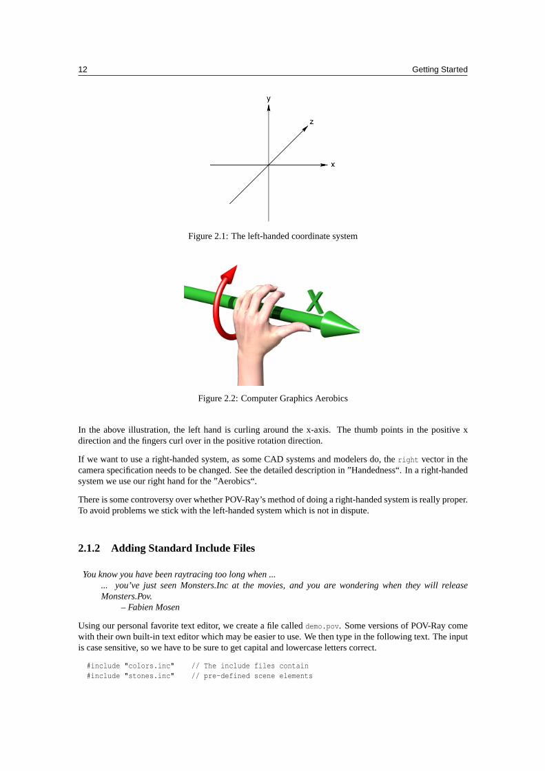
First, we have to tell POV-Ray where our camera is and where it is looking. To do this, we use 3Dcoordinates. The usual coordinate system for POV-Ray has the positive y-axis pointing up, the positivex-axis pointing to the right, and the positive z-axis pointing into the screen as follows:
This kind of coordinate system is called a left-handed coordinate system. If we use our left hand’s fingerswe can easily see why it is called left-handed. We just point our thumb in the direction of the positive x-axis(to the right), the index finger in the direction of the positive y-axis (straight up) and the middle finger in thepositive z-axis direction (forward). We can only do this with our left hand. If we had used our right handwe would not have been able to point the middle finger in the correct direction.
The left hand can also be used to determine rotation directions. To do this we must perform the famous”Computer Graphics Aerobics“ exercise. We hold up our left hand and point our thumb in the positivedirection of the axis of rotation. Our fingers will curl in the positive direction of rotation. Similarly if wepoint our thumb in the negative direction of the axis our fingers will curl in the negative direction of rotation.
12 Getting Started
Figure 2.1: The left-handed coordinate system
Figure 2.2: Computer Graphics Aerobics
In the above illustration, the left hand is curling around the x-axis. The thumb points in the positive xdirection and the fingers curl over in the positive rotation direction.
If we want to use a right-handed system, as some CAD systems and modelers do, theright vector in thecamera specification needs to be changed. See the detailed description in ”Handedness“. In a right-handedsystem we use our right hand for the ”Aerobics“.
There is some controversy over whether POV-Ray’s method of doing a right-handed system is really proper.To avoid problems we stick with the left-handed system which is not in dispute.
2.1.2 Adding Standard Include Files
You know you have been raytracing too long when ...... you’ve just seen Monsters.Inc at the movies, and you are wondering when they will releaseMonsters.Pov.
– Fabien Mosen
Using our personal favorite text editor, we create a file calleddemo.pov. Some versions of POV-Ray comewith their own built-in text editor which may be easier to use. We then type in the following text. The inputis case sensitive, so we have to be sure to get capital and lowercase letters correct.
#include "colors.inc" // The include files contain#include "stones.inc" // pre-defined scene elements
2.1 Our First Image 13
The first include statement reads in definitions for various useful colors. The second include statement readsin a collection of stone textures. POV-Ray comes with many standard include files. Others of interest are:
#include "textures.inc" // pre-defined scene elements#include "shapes.inc"#include "glass.inc"#include "metals.inc"#include "woods.inc"
They read pre-defined textures, shapes, glass, metal, and wood textures. It is a good idea to have a lookthrough them to see a few of the many possible shapes and textures available.
We should only include files we really need in our scene. Some of the include files coming with POV-Rayare quite large and we should better save the parsing time and memory if we do not need them. In thefollowing examples we will only use thecolors.inc, andstones.inc include files.
We may have as many include files as needed in a scene file. Include files may themselves contain includefiles, but we are limited to declaring includes nested only ten levels deep.
Filenames specified in the include statements will be searched for in the current directory first. If it fails tofind your .Inc files in the current directory, POV-Ray searches any “library paths” that you have specified.Library paths are options set by the+L command-line switch orLibrary Path option. See the chapter“Setting POV-Ray Options” for more information on library paths.
Because it is more useful to keep include files in a separate directory, standard installations of POV-Rayplace these files in the c:\povray3\include directory (replace ’c:\povray3’ with the actual directory thatyou installed POV-Ray in). If you get an error message saying that POV-Ray cannot open “colors.inc” orother include files, make sure that you specify the library path properly.
2.1.3 Adding a Camera
Thecamera statement describes where and how the camera sees the scene. It gives x-, y- and z-coordinates toindicate the position of the camera and what part of the scene it is pointing at. We describe the coordinatesusing a three-partvector. A vector is specified by putting three numeric values between a pair of anglebrackets and separating the values with commas. We add the following camera statement to the scene.
camera {location <0, 2, -3>look_at <0, 1, 2>
}
Briefly, location <0,2,-3> places the camera up two units and back three units from the center of theray-tracing universe which is at<0,0,0>. By default +z is into the screen and -z is back out of the screen.
Also look at <0,1,2> rotates the camera to point at the coordinates<0,1,2>. A point 1 unit up from theorigin and 2 units away from the origin. This makes it 5 units in front of and 1 unit lower than the camera.Thelook at point should be the center of attention of our image.
2.1.4 Describing an Object
Now that the camera is set up to record the scene, let’s place a yellow sphere into the scene. We add thefollowing to our scene file:
sphere {<0, 1, 2>, 2texture {
pigment { color Yellow }
14 Getting Started
}}
The first vector specifies the center of the sphere. In this example the x coordinate is zero so it is centeredleft and right. It is also at y=1 or one unit up from the origin. The z coordinate is 2 which is five units infront of the camera, which is at z=-3. After the center vector is a comma followed by the radius which inthis case is two units. Since the radius is half the width of a sphere, the sphere is four units wide.
2.1.5 Adding Texture to an Object
After we have defined the location and size of the sphere, we need to describe the appearance of the surface.Thetexture statement specifies these parameters. Texture blocks describe the color, bumpiness and finishproperties of an object. In this example we will specify the color only. This is the minimum we must do.All other texture options except color will use default values.
The color we define is the way we want an object to look if fully illuminated. If we were painting a pictureof a sphere we would use dark shades of a color to indicate the shadowed side and bright shades on theilluminated side. However ray-tracing takes care of that for you. We only need to pick the basic colorinherent in the object and POV-Ray brightens or darkens it depending on the lighting in the scene. Becausewe are defining the basic color the object actuallyhas rather than how itlooks the parameter is calledpigment.
Many types of color patterns are available for use in a pigment statement. The keywordcolor specifies thatthe whole object is to be one solid color rather than some pattern of colors. We can use one of the coloridentifiers previously defined in the standard include filecolors.inc.
If no standard color is available for our needs, we may define our own color by using the color keywordfollowed byred, green, and blue keywords specifying the amount of red, green and blue to be mixed. Forexample a nice shade of pink can be specified by:
color red 1.0 green 0.8 blue 0.8
Note: the international - rather than American - form “colour” is also acceptable and may be used anywherethat “color” may be used.
The values after each keyword should be in the range from 0.0 to 1.0. Any of the three components notspecified will default to 0. A shortcut notation may also be used. The following produces the same shadeof pink:
color rgb <1.0, 0.8, 0.8>
In many cases thecolor keyword is superfluous, so the shortest way to specify the pink color is:
rgb <1.0, 0.8, 0.8>
Colors are explained in more detail in section “Specifying Colors”.
2.1.6 Defining a Light Source
One more detail is needed for our scene. We need a light source. Until we create one, there is no light inthis virtual world. Thus we add the line
light_source { <2, 4, -3> color White}
to the scene file to get our first complete POV-Ray scene file as shown below.
#include "colors.inc"background { color Cyan }camera {
2.2 Basic Shapes 15
location <0, 2, -3>look_at <0, 1, 2>
}sphere {
<0, 1, 2>, 2texture {
pigment { color Yellow }}
}light_source { <2, 4, -3> color White}
The vector in thelight source statement specifies the location of the light as two units to our right, fourunits above the origin and three units back from the origin. The light source is an invisible tiny point thatemits light. It has no physical shape, so no texture is needed.
That’s it! We close the file and render a small picture of it using whatever methods you used for yourparticular platform. If you specified a preview display it will appear on your screen. If you specified anoutput file (the default is file output on), then POV-Ray also created a file.
Note: if you do not have high color or true color display hardware then the preview image may look poorbut the full detail is written to the image file regardless of the type of display.
The scene we just traced is not quite state of the art but we will have to start with the basics before we soonget to much more fascinating features and scenes.
2.2 Basic Shapes
So far we have just used the sphere shape. There are many other types of shapes that can be rendered byPOV-Ray. The following sections will describe how to use some of the more simple objects as a replacementfor the sphere used above.
2.2.1 Box Object
Thebox is one of the most common objects used. We try this example in place of the sphere:
box {<-1, 0, -1>, // Near lower left corner< 1, 0.5, 3> // Far upper right cornertexture {
T_Stone25 // Pre-defined from stones.incscale 4 // Scale by the same amount in all
// directions}rotate y*20 // Equivalent to "rotate <0,20,0>"
}
In the example we can see that a box is defined by specifying the 3D coordinates of its opposite corners. Thefirst vector is generally the minimum x-, y- and z-coordinates and the 2nd vector should be the maximumx-, y- and z-values however any two opposite corners may be used. Box objects can only be defined parallelto the axes of the world coordinate system. We can later rotate them to any angle.
Note: we can perform simple math on values and vectors. In the rotate parameter we multiplied the vectoridentifiery by 20. This is the same as<0,1,0>*20 or <0,20,0>.
16 Getting Started
2.2.2 Cone Object
Here is another example showing how to use acone:
cone {<0, 1, 0>, 0.3 // Center and radius of one end<1, 2, 3>, 1.0 // Center and radius of other endtexture { T_Stone25 scale 4 }
}
The cone shape is defined by the center and radius of each end. In this example one end is at location<0,1,0> and has a radius of 0.3 while the other end is centered at<1,2,3> with a radius of 1. If we wantthe cone to come to a sharp point we must use radius=0. The solid end caps are parallel to each other andperpendicular to the cone axis. If we want an open cone with no end caps we have to add the keywordopen
after the 2nd radius like this:
cone {<0, 1, 0>, 0.3 // Center and radius of one end<1, 2, 3>, 1.0 // Center and radius of other endopen // Removes end capstexture { T_Stone25 scale 4 }
}
2.2.3 Cylinder Object
We may also define acylinder like this:
cylinder {<0, 1, 0>, // Center of one end<1, 2, 3>, // Center of other end0.5 // Radiusopen // Remove end capstexture { T_Stone25 scale 4 }
}
2.2.4 Plane Object
Let’s try out a computer graphics standard“The Checkered Floor”.We add the following object to the firstversion of thedemo.pov file, the one including the sphere.
plane { <0, 1, 0>, -1pigment {
checker color Red, color Blue}
}
The object defined here is an infinite plane. The vector<0,1,0> is the surface normal of the plane (i.e. ifwe were standing on the surface, the normal points straight up). The number afterward is the distance thatthe plane is displaced along the normal from the origin – in this case, the floor is placed at y=-1 so that thesphere at y=1, radius=2, is resting on it.
Note: even though there is notexture statement there is an implied texture here. We might find thatcontinually typing statements that are nested liketexture {pigment} can get to be tiresome so POV-Raylet’s us leave out thetexture statement under many circumstances. In general we only need the textureblock surrounding a texture identifier (like theT Stone25 example above), or when creating layered textures(which are covered later).
2.2 Basic Shapes 17
This pigment uses the checker color pattern and specifies that the two colors red and blue should be used.
Because the vectors<1,0,0>, <0,1,0> and<0,0,1> are used frequently, POV-Ray has three built-in vectoridentifiers x, y andz respectively that can be used as a shorthand. Thus the plane could be defined as:
plane { y, -1pigment { ... }
}
Note: that we do not use angle brackets around vector identifiers.
Looking at the floor, we notice that the ball casts a shadow on the floor. Shadows are calculated veryaccurately by the ray-tracer, which creates precise, sharp shadows. In the real world, penumbral or “soft”shadows are often seen. Later we will learn how to use extended light sources to soften the shadows.
2.2.5 Torus Object
A torus can be thought of as a donut or an inner-tube. It is a shape that is vastly useful in many kinds ofCSG so POV-Ray has adopted this 4th order quartic polynomial as a primitive shape. The syntax for a torusis so simple that it makes it a very easy shape to work with once we learn what the two float values mean.Instead of a lecture on the subject, let’s create one and do some experiments with it.
We create a file calledtordemo.pov and edit it as follows:
#include "colors.inc"camera {
location <0, .1, -25>look_at 0angle 30
}background { color Gray50 } // to make the torus easy to seelight_source { <300, 300, -1000> White }torus {
4, 1 // major and minor radiusrotate -90*x // so we can see it from the toppigment { Green }
}
We trace the scene. Well, it is a donut alright. Let’s try changing the major and minor radius values and seewhat happens. We change them as follows:
torus { 5, .25 // major and minor radius
That looks more like a hula-hoop! Let’s try this:
torus { 3.5, 2.5 // major and minor radius
Whoa! A donut with a serious weight problem!
With such a simple syntax, there is not much else we can do to a torus besides change its texture... or isthere? Let’s see...
Tori are very useful objects in CSG. Let’s try a little experiment. We make a difference of a torus and a box:
difference {torus {
4, 1rotate x*-90 // so we can see it from the top
}box { <-5, -5, -1>, <5, 0, 1> }pigment { Green }
18 Getting Started
}
Interesting... a half-torus. Now we add another one flipped the other way. Only, let’s declare the originalhalf-torus and the necessary transformations so we can use them again:
#declare Half_Torus = difference {torus {
4, 1rotate -90*x // so we can see it from the top
}box { <-5, -5, -1>, <5, 0, 1> }pigment { Green }
}#declare Flip_It_Over = 180*x;#declare Torus_Translate = 8; // twice the major radius
Now we create a union of twoHalf Torus objects:
union {object { Half_Torus }object { Half_Torus
rotate Flip_It_Overtranslate Torus_Translate*x
}}
This makes an S-shaped object, but we cannot see the whole thing from our present camera. Let’s add a fewmore links, three in each direction, move the object along the +z-direction and rotate it about the +y-axis sowe can see more of it. We also notice that there appears to be a small gap where the half Tori meet. This isdue to the fact that we are viewing this scene from directly on the x-z-plane. We will change the camera’sy-coordinate from 0 to 0.1 to eliminate this.
union {object { Half_Torus }object { Half_Torus
rotate Flip_It_Overtranslate x*Torus_Translate
}object { Half_Torus
translate x*Torus_Translate*2}object { Half_Torus
rotate Flip_It_Overtranslate x*Torus_Translate*3
}object { Half_Torus
rotate Flip_It_Overtranslate -x*Torus_Translate
}object { Half_Torus
translate -x*Torus_Translate*2}object { Half_Torus
rotate Flip_It_Overtranslate -x*Torus_Translate*3
}object { Half_Torus
translate -x*Torus_Translate*4}rotate y*45
2.2 Basic Shapes 19
translate z*20}
Rendering this we see a cool, undulating, snake-like something-or-other. Neato. But we want to modelsomething useful, something that we might see in real life. How about a chain?
Thinking about it for a moment, we realize that a single link of a chain can be easily modeled using twohalf tori and two cylinders. We create a new file. We can use the same camera, background, light sourceand declared objects and transformations as we used intordemo.pov:
#include "colors.inc"camera {
location <0, .1, -25>look_at 0angle 30
}background { color Gray50 }light_source{ <300, 300, -1000> White }#declare Half_Torus = difference {
torus {4,1sturmrotate x*-90 // so we can see it from the top
}box { <-5, -5, -1>, <5, 0, 1> }pigment { Green }
}#declare Flip_It_Over = x*180;#declare Torus_Translate = 8;
Now, we make a complete torus of two half tori:
union {object { Half_Torus }object { Half_Torus rotate Flip_It_Over }
}
This may seem like a wasteful way to make a complete torus, but we are really going to move each halfapart to make room for the cylinders. First, we add the declared cylinder before the union:
#declare Chain_Segment = cylinder {<0, 4, 0>, <0, -4, 0>, 1pigment { Green }
}
We then add twoChain Segments to the union and translate them so that they line up with the minor radiusof the torus on each side:
union {object { Half_Torus }object { Half_Torus rotate Flip_It_Over }object { Chain_Segment translate x*Torus_Translate/2 }object { Chain_Segment translate -x*Torus_Translate/2 }
}
Now we translate the two half tori +y and -y so that the clipped ends meet the ends of the cylinders. Thisdistance is equal to half of the previously declaredTorus Translate:
union {object {
Half_Torustranslate y*Torus_Translate/2
20 Getting Started
}object {Half_Torusrotate Flip_It_Overtranslate -y*Torus_Translate/2
}object {
Chain_Segmenttranslate x*Torus_Translate/2
}object {
Chain_Segmenttranslate -x*Torus_Translate/2
}}
We render this and voila! A single link of a chain. But we are not done yet! Whoever heard of a greenchain? We would rather use a nice metallic color instead. First, we remove any pigment blocks in thedeclared tori and cylinders. Then we add a declaration for a golden texture just before the union that createsthe link. Finally, we add the texture to the union and declare it as a single link:
#declare Half_Torus = difference {torus {
4,1sturmrotate x*-90 // so we can see it from the top
}box { <-5, -5, -1>, <5, 0, 1> }
}
#declare Chain_Segment = cylinder {<0, 4, 0>, <0, -4, 0>, 1
}
#declare Chain_Gold = texture {pigment { BrightGold }finish {
ambient .1diffuse .4reflection .25specular 1metallic
}}
#declare Link = union {object {
Half_Torustranslate y*Torus_Translate/2
}object {
Half_Torusrotate Flip_It_Overtranslate -y*Torus_Translate/2
}object {
Chain_Segmenttranslate x*Torus_Translate/2
2.2 Basic Shapes 21
}object {Chain_Segmenttranslate -x*Torus_Translate/2
} texture { Chain_Gold }}
Now we make a union of two links. The second one will have to be translated +y so that its inner wall justmeets the inner wall of the other link, just like the links of a chain. This distance turns out to be doublethe previously declaredTorus Translate minus 2 (twice the minor radius). This can be described by theexpression:
Torus_Translate*2-2*y
We declare this expression as follows:
#declare Link_Translate = Torus_Translate*2-2*y;
In the object block, we will use this declared value so that we can multiply it to create other links. Now, werotate the second link90*y so that it is perpendicular to the first, just like links of a chain. Finally, we scalethe union by 1/4 so that we can see the whole thing:
union {object { Link }object { Link translate y*Link_Translate rotate y*90 }scale .25
}
We render this and we will see a very realistic pair of links. If we want to make an entire chain, we mustdeclare the above union and then create another union of this declared object. We must be sure to removethe scaling from the declared object:
#declare Link_Pair =union {
object { Link }object { Link translate y*Link_Translate rotate y*90 }
}
Now we declare our chain:
#declare Chain = union {object { Link_Pair}object { Link_Pair translate y*Link_Translate*2 }object { Link_Pair translate y*Link_Translate*4 }object { Link_Pair translate y*Link_Translate*6 }object { Link_Pair translate -y*Link_Translate*2 }object { Link_Pair translate -y*Link_Translate*4 }object { Link_Pair translate -y*Link_Translate*6 }
}
And finally we create our chain with a couple of transformations to make it easier to see. These includescaling it down by a factor of 1/10, and rotating it so that we can clearly see each link:
object { Chain scale .1 rotate <0, 45, -45> }
We render this and we should see a very realistic gold chain stretched diagonally across the screen.
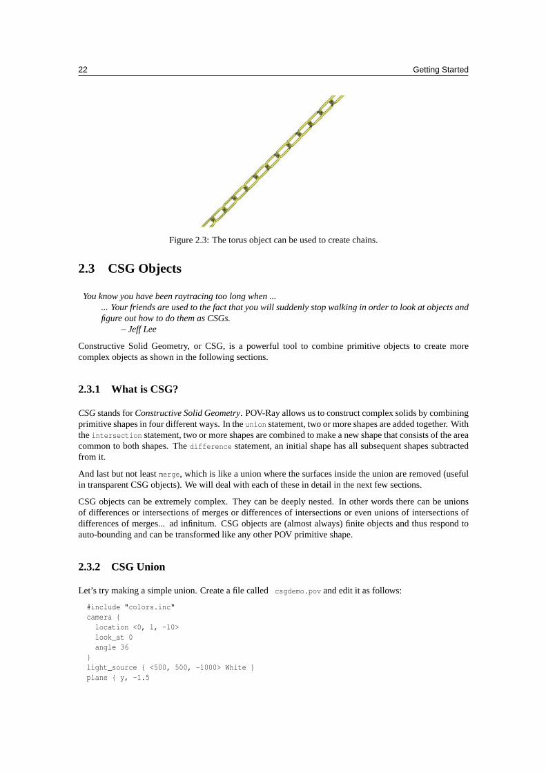
22 Getting Started
Figure 2.3: The torus object can be used to create chains.
2.3 CSG Objects
You know you have been raytracing too long when ...... Your friends are used to the fact that you will suddenly stop walking in order to look at objects andfigure out how to do them as CSGs.
– Jeff Lee
Constructive Solid Geometry, or CSG, is a powerful tool to combine primitive objects to create morecomplex objects as shown in the following sections.
2.3.1 What is CSG?
CSGstands forConstructive Solid Geometry. POV-Ray allows us to construct complex solids by combiningprimitive shapes in four different ways. In theunion statement, two or more shapes are added together. Withtheintersection statement, two or more shapes are combined to make a new shape that consists of the areacommon to both shapes. Thedifference statement, an initial shape has all subsequent shapes subtractedfrom it.
And last but not leastmerge, which is like a union where the surfaces inside the union are removed (usefulin transparent CSG objects). We will deal with each of these in detail in the next few sections.
CSG objects can be extremely complex. They can be deeply nested. In other words there can be unionsof differences or intersections of merges or differences of intersections or even unions of intersections ofdifferences of merges... ad infinitum. CSG objects are (almost always) finite objects and thus respond toauto-bounding and can be transformed like any other POV primitive shape.
2.3.2 CSG Union
Let’s try making a simple union. Create a file calledcsgdemo.pov and edit it as follows:
#include "colors.inc"camera {
location <0, 1, -10>look_at 0angle 36
}light_source { <500, 500, -1000> White }plane { y, -1.5
2.3 CSG Objects 23
pigment { checker Green White }}
Let’s add two spheres each translated 0.5 units along the x-axis in each direction. We color one blue andthe other red.
sphere { <0, 0, 0>, 1pigment { Blue }translate -0.5*x
}sphere { <0, 0, 0>, 1
pigment { Red }translate 0.5*x
}
We trace this file and note the results. Now we place a union block around the two spheres. This will createa single CSG union out of the two objects.
union{sphere { <0, 0, 0>, 1
pigment { Blue }translate -0.5*x
}sphere { <0, 0, 0>, 1
pigment { Red }translate 0.5*x
}}
We trace the file again. The union will appear no different from what each sphere looked like on its own,but now we can give the entire union a single texture and transform it as a whole. Let’s do that now.
union{sphere { <0, 0, 0>, 1
translate -0.5*x}sphere { <0, 0, 0>, 1
translate 0.5*x}pigment { Red }scale <1, .25, 1>rotate <30, 0, 45>
}
We trace the file again. As we can see, the object has changed dramatically. We experiment with differentvalues of scale and rotate and try some different textures.
There are many advantages of assigning only one texture to a CSG object instead of assigning the textureto each individual component. First, it is much easier to use one texture if our CSG object has a lot ofcomponents because changing the objects appearance involves changing only one single texture. Second,the file parses faster because the texture has to be parsed only once. This may be a great factor when doinglarge scenes or animations. Third, using only one texture saves memory because the texture is only storedonce and referenced by all components of the CSG object. Assigning the texture to all n components meansthat it is stored n times.
2.3.3 CSG Intersection
Now let’s use these same spheres to illustrate theintersection CSG object. We change the wordunion tointersection and delete thescale androtate statements:
24 Getting Started
intersection {sphere { <0, 0, 0>, 1
translate -0.5*x}sphere { <0, 0, 0>, 1
translate 0.5*x}pigment { Red }
}
We trace the file and will see a lens-shaped object instead of the two spheres. This is because an intersectionconsists of the area shared by both shapes, in this case the lens-shaped area where the two spheres overlap.We like this lens-shaped object so we will use it to demonstrate differences.
2.3.4 CSG Difference
We rotate the lens-shaped intersection about the y-axis so that the broad side is facing the camera.
intersection{sphere { <0, 0, 0>, 1
translate -0.5*x}sphere { <0, 0, 0>, 1
translate 0.5*x}pigment { Red }rotate 90*y
}
Let’s create a cylinder and stick it right in the middle of the lens.
cylinder { <0, 0, -1> <0, 0, 1>, .35pigment { Blue }
}
We render the scene to see the position of the cylinder. We will place adifference block around both thelens-shaped intersection and the cylinder like this:
difference {intersection {
sphere { <0, 0, 0>, 1translate -0.5*x
}sphere { <0, 0, 0>, 1
translate 0.5*x}pigment { Red }rotate 90*y
}cylinder { <0, 0, -1> <0, 0, 1>, .35
pigment { Blue }}
}
We render the file again and see the lens-shaped intersection with a neat hole in the middle of it where thecylinder was. The cylinder has beensubtracted from the intersection. Note that the pigment of the cylindercauses the surface of the hole to be colored blue. If we eliminate this pigment the surface of the hole willbe black, as this is the default color if no color is specified.
2.3 CSG Objects 25
OK, let’s get a little wilder now. Let’s declare our perforated lens object to give it a name. Let’s alsoeliminate all textures in the declared object because we will want them to be in the final union instead.
#declare Lens_With_Hole = difference {intersection {
sphere { <0, 0, 0>, 1translate -0.5*x
}sphere { <0, 0, 0>, 1
translate 0.5*x}rotate 90*y
}cylinder { <0, 0, -1> <0, 0, 1>, .35 }
}
Let’s use a union to build a complex shape composed of copies of this object.
union {object { Lens_With_Hole translate <-.65, .65, 0> }object { Lens_With_Hole translate <.65, .65, 0> }object { Lens_With_Hole translate <-.65, -.65, 0> }object { Lens_With_Hole translate <.65, -.65, 0> }pigment { Red }
}
We render the scene. An interesting object to be sure. But let’s try something more. Let’s make it apartially-transparent object by adding some filter to the pigment block.
union {object { Lens_With_Hole translate <-.65, .65, 0> }object { Lens_With_Hole translate <.65, .65, 0> }object { Lens_With_Hole translate <-.65, -.65, 0> }object { Lens_With_Hole translate <.65, -.65, 0> }pigment { Red filter .5 }
}
We render the file again. This looks pretty good... only... we can see parts of each of the lens objects insidethe union! This is not good.
2.3.5 CSG Merge
This brings us to the fourth kind of CSG object, themerge. Merges are the same as unions, but the geometryof the objects in the CSG that is inside the merge is not traced. This should eliminate the problem with ourobject. Let’s try it.
merge {object { Lens_With_Hole translate <-.65, .65, 0> }object { Lens_With_Hole translate <.65, .65, 0> }object { Lens_With_Hole translate <-.65, -.65, 0> }object { Lens_With_Hole translate <.65, -.65, 0> }pigment { Red filter .5 }
}
Sure enough, it does!
26 Getting Started
2.3.6 CSG Pitfalls
There is a severe pitfall in the CSG code that we have to be aware of.
Co-incident Surfaces
POV-Ray uses inside/outside tests to determine the points at which a ray intersects a CSG object. A problemarises when the surfaces of two different shapes coincide because there is no way (due to the computer’sfloating-point accuracy) to tell whether a point on the coincident surface belongs to one shape or the other.
Look at the following example where a cylinder is used to cut a hole in a larger box.
difference {box { -1, 1 pigment { Red } }cylinder { -z, z, 0.5 pigment { Green } }
}
Note: that the vectors -1 and 1 in the box definition expand to<-1,-1,-1> and<1,1,1> respectively.
If we trace this object we see red speckles where the hole is supposed to be. This is caused by the coincidentsurfaces of the cylinder and the box. One time the cylinder’s surface is hit first by a viewing ray, resultingin the correct rendering of the hole, and another time the box is hit first, leading to a wrong result where thehole vanishes and red speckles appear. This problem can be avoided by increasing the size of the cylinderto get rid of the coincidence surfaces. This is done by:
difference {box { -1, 1 pigment { Red } }cylinder { -1.001*z, 1.001*z, 0.5 pigment { Green } }
}
In general we have to make the subtracted object a little bit larger in a CSG difference. We just have to lookfor coincident surfaces and increase the subtracted object appropriately to get rid of those surfaces.
The same problem occurs in CSG intersections and is also avoided by scaling some of the involved objects.
2.4 The Light Source
You know you have been raytracing too long when ...... You take a photo course just to learn how to get the lighting right.
– Christoph Rieder
In any ray-traced scene, the light needed to illuminate our objects and their surfaces must come from a lightsource. There are many kinds of light sources available in POV-Ray and careful use of the correct kind canyield very impressive results. Let’s take a moment to explore some of the different kinds of light sourcesand their various parameters.
2.4.1 The Pointlight Source
Pointlights are exactly what the name indicates. A pointlight has no size, is invisible and illuminateseverything in the scene equally no matter how far away from the light source it may be (this behaviorcan be changed). This is the simplest and most basic light source. There are only two important parameters,location and color. Let’s design a simple scene and place a pointlight source in it.
We create a new file and name itlitedemo.pov. We edit it as follows:
2.4 The Light Source 27
#include "colors.inc"#include "textures.inc"camera {
location <-4, 3, -9>look_at <0, 0, 0>angle 48
}
We add the following simple objects:
plane {y, -1texture {
pigment {checkercolor rgb<0.5, 0, 0>color rgb<0, 0.5, 0.5>
}finish {
diffuse 0.4ambient 0.2phong 1phong_size 100reflection 0.25
}}
}torus {
1.5, 0.5texture { Brown_Agate }rotate <90, 160, 0>translate <-1, 1, 3>
}box {
<-1, -1, -1>, <1, 1, 1>texture { DMFLightOak }translate <2, 0, 2.3>
}cone {
<0,1,0>, 0, <0,0,0>, 1texture { PinkAlabaster }scale <1, 3, 1>translate <-2, -1, -1>
}sphere {
<0,0,0>,1texture { Sapphire_Agate }translate <1.5, 0, -2>
}
Now we add a pointlight:
light_source {<2, 10, -3>color White
}
We render this at 200x150-A and see that the objects are clearly visible with sharp shadows. The sides ofcurved objects nearest the light source are brightest in color with the areas that are facing away from the
28 Getting Started
light source being darkest. We also note that the checkered plane is illuminated evenly all the way to thehorizon. This allows us to see the plane, but it is not very realistic.
2.4.2 The Spotlight Source
Spotlights are a very useful type of light source. They can be used to add highlights and illuminate featuresmuch as a photographer uses spots to do the same thing. To create a spotlight simply add thespotlight
keyword to a regular point light. There are a few more parameters with spotlights than with pointlights.These areradius, falloff, tightness andpoint at. Theradius parameter is the angle of the fully illumi-nated cone. Thefalloff parameter is the angle of theumbracone where the light falls off to darkness. Thetightness is a parameter that determines the rate of the light falloff. Thepoint at parameter is just what itsays, the location where the spotlight is pointing to. Let’s change the light in our scene as follows:
light_source {<0, 10, -3>color Whitespotlightradius 15falloff 20tightness 10point_at <0, 0, 0>
}
We render this at 200x150-A and see that only the objects are illuminated. The rest of the plane and theouter portions of the objects are now unlit. There is a broad falloff area but the shadows are still razor sharp.Let’s try fiddling with some of these parameters to see what they do. We change the falloff value to 16 (itmust always be larger than the radius value) and render again. Now the falloff is very narrow and the objectsare either brightly lit or in total darkness. Now we change falloff back to 20 and change the tightness valueto 100 (higher is tighter) and render again. The spotlight appears to have gotten much smaller but what hasreally happened is that the falloff has become so steep that the radius actually appears smaller.
We decide that a tightness value of 10 (the default) and a falloff value of 18 are best for this spotlight andwe now want to put a few spots around the scene for effect. Let’s place a slightly narrower blue and a redone in addition to the white one we already have:
light_source {<10, 10, -1>color Redspotlightradius 12falloff 14tightness 10point_at <2, 0, 0>
}light_source {
<-12, 10, -1>color Bluespotlightradius 12falloff 14tightness 10point_at <-2, 0, 0>
}
Rendering this we see that the scene now has a wonderfully mysterious air to it. The three spotlights allconverge on the objects making them blue on one side and red on the other with enough white in the middleto provide a balance.
2.4 The Light Source 29
2.4.3 The Cylindrical Light Source
Spotlights are cone shaped, meaning that their effect will change with distance. The farther away from thespotlight an object is, the larger the apparent radius will be. But we may want the radius and falloff to be aparticular size no matter how far away the spotlight is. For this reason, cylindrical light sources are needed.A cylindrical light source is just like a spotlight, except that the radius and falloff regions are the same nomatter how far from the light source our object is. The shape is therefore a cylinder rather than a cone. Wecan specify a cylindrical light source by replacing thespotlight keyword with thecylinder keyword. Wetry this now with our scene by replacing all three spotlights with cylinder lights and rendering again. Wesee that the scene is much dimmer. This is because the cylindrical constraints do not let the light spread outlike in a spotlight. Larger radius and falloff values are needed to do the job. We try a radius of 20 and afalloff of 30 for all three lights. That’s the ticket!
2.4.4 The Area Light Source
You know you have been raytracing too long when ...... You wear fuzzy clothing to soften your shadow.
– Mark Kadela
So far all of our light sources have one thing in common. They produce sharp shadows. This is because theactual light source is a point that is infinitely small. Objects are either in direct sight of the light, in whichcase they are fully illuminated, or they are not, in which case they are fully shaded. In real life, this kindof stark light and shadow situation exists only in outer space where the direct light of the sun pierces thetotal blackness of space. But here on Earth, light bends around objects, bounces off objects, and usuallythe source has some dimension, meaning that it can be partially hidden from sight (shadows are not sharpanymore). They have what is known as anumbra, or an area of fuzziness where there is neither total light orshade. In order to simulate thesesoftshadows, a ray-tracer must give its light sources dimension. POV-Rayaccomplishes this with a feature known as an area light.
Area lights have dimension in two axis’. These are specified by the first two vectors in the area light syntax.We must also specify how many lights are to be in the array. More will give us cleaner soft shadows butwill take longer to render. Usually a 3*3 or a 5*5 array will suffice. We also have the option of specifyingan adaptive value. Theadaptive keyword tells the ray-tracer that it can adapt to the situation and sendonly the needed rays to determine the value of the pixel. If adaptive is not used, a separate ray will besent for every light in the area light. This can really slow things down. The higher the adaptive value thecleaner the umbra will be but the longer the trace will take. Usually an adaptive value of 1 is sufficient.Finally, we probably should use thejitter keyword. This tells the ray-tracer to slightly move the positionof each light in the area light so that the shadows appear truly soft instead of giving us an umbra consistingof closely banded shadows.
OK, let’s try one. We comment out the cylinder lights and add the following:
light_source {<2, 10, -3>color Whitearea_light <5, 0, 0>, <0, 0, 5>, 5, 5adaptive 1jitter
}
This is a white area light centered at<2,10,-3>. It is 5 units (along the x-axis) by 5 units (along the z-axis)in size and has 25 (5*5) lights in it. We have specified adaptive 1 and jitter. We render this at 200x150-A.
Right away we notice two things. The trace takes quite a bit longer than it did with a point or a spotlightand the shadows are no longer sharp! They all have nice soft umbrae around them. Wait, it gets better.
30 Getting Started
Spotlights and cylinder lights can be area lights too! Remember those sharp shadows from the spotlights inour scene? It would not make much sense to use a 5*5 array for a spotlight, but a smaller array might do agood job of giving us just the right amount of umbra for a spotlight. Let’s try it. We comment out the arealight and change the cylinder lights so that they read as follows:
light_source {<2, 10, -3>color Whitespotlightradius 15falloff 18tightness 10area_light <1, 0, 0>, <0, 0, 1>, 2, 2adaptive 1jitterpoint_at <0, 0, 0>
}light_source {
<10, 10, -1>color Redspotlightradius 12falloff 14tightness 10area_light <1, 0, 0>, <0, 0, 1>, 2, 2adaptive 1jitterpoint_at <2, 0, 0>
}light_source {
<-12, 10, -1>color Bluespotlightradius 12falloff 14tightness 10area_light <1, 0, 0>, <0, 0, 1>, 2, 2adaptive 1jitterpoint_at <-2, 0, 0>
}
We now have three area-spotlights, one unit square consisting of an array of four (2*2) lights, three differentcolors, all shining on our scene. We render this at 200x150-A. It appears to work perfectly. All our shadowshave small, tight umbrae, just the sort we would expect to find on an object under a real spotlight.
2.4.5 The Ambient Light Source
The ambient light sourceis used to simulate the effect of inter-diffuse reflection. If there was not inter-diffuse reflection all areas not directly lit by a light source would be completely dark. POV-Ray uses theambient keyword to determine how much light coming from the ambient light source is reflected by asurface.
By default the ambient light source, which emits its light everywhere and in all directions, is pure white(rgb <1,1,1>). Changing its color can be used to create interesting effects. First of all the overall lightlevel of the scene can be adjusted easily. Instead of changing all ambient values in every finish only the
2.4 The Light Source 31
ambient light source is modified. By assigning different colors we can create nice effects like a moodyreddish ambient lighting. For more details about the ambient light source see “Ambient Light”.
Below is an example of a red ambient light source.
global_settings { ambient_light rgb<1, 0, 0> }
2.4.6 Light Source Specials
Using Shadowless Lights
Light sources can be assigned theshadowless keyword and no shadows will be cast due to its presence in ascene. Sometimes, scenes are difficult to illuminate properly using the lights we have chosen to illuminateour objects. It is impractical and unrealistic to apply a higher ambient value to the texture of every object inthe scene. So instead, we would place a couple offill lights around the scene. Fill lights are simply dimmerlights with theshadowless keyword that act to boost the illumination of other areas of the scene that maynot be lit well. Let’s try using one in our scene.
Remember the three colored area spotlights? We go back and un-comment them and comment out any otherlights we have made. Now we add the following:
light_source {<0, 20, 0>color Gray50shadowless
}
This is a fairly dim light 20 units over the center of the scene. It will give a dim illumination to all objectsincluding the plane in the background. We render it and see.
Assigning an Object to a Light Source
Light sources are invisible. They are just a location where the light appears to be coming from. They haveno true size or shape. If we want our light source to be a visible shape, we can use thelooks like keyword.We can specify that our light source can look like any object we choose. When we uselooks like, thenno -
shadow is applied to the object automatically. This is done so that the object will not block any illuminationfrom the light source. If we want some blocking to occur (as in a lamp shade), it is better to simply use aunion to do the same thing. Let’s add such an object to our scene. Here is a light bulb we have made justfor this purpose:
#declare Lightbulb = union {merge {
sphere { <0,0,0>,1 }cylinder {
<0,0,1>, <0,0,0>, 1scale <0.35, 0.35, 1.0>translate 0.5*z
}texture {
pigment {color rgb <1, 1, 1>}finish {ambient .8 diffuse .6}
}}cylinder {
<0,0,1>, <0,0,0>, 1scale <0.4, 0.4, 0.5>
32 Getting Started
texture { Brass_Texture }translate 1.5*z
}rotate -90*xscale .5
}
Now we add the light source:
light_source {<0, 2, 0>color Whitelooks_like { Lightbulb }
}
Rendering this we see that a fairly believable light bulb now illuminates the scene. However, if we do notspecify a high ambient value, the light bulb is not lit by the light source. On the plus side, all of the shadowsfall away from the light bulb, just as they would in a real situation. The shadows are sharp, so let’s makeour bulb an area light:
light_source {<0, 2, 0>color Whitearea_light <1, 0, 0>, <0, 1, 0>, 2, 2adaptive 1jitterlooks_like { Lightbulb }
}
We note that we have placed this area light in the x-y-plane instead of the x-z-plane. We also note thatthe actual appearance of the light bulb is not affected in any way by the light source. The bulb must beilluminated by some other light source or by, as in this case, a high ambient value.
Using Light Fading
If it is realism we want, it is not realistic for the plane to be evenly illuminated off into the distance. In reallife, light gets scattered as it travels so it diminishes its ability to illuminate objects the farther it gets fromits source. To simulate this, POV-Ray allows us to use two keywords:fade distance, which specifies thedistance at which full illumination is achieved, andfade power, an exponential value which determines theactual rate of attenuation. Let’s apply these keywords to our fill light.
First, we make the fill light a little brighter by changingGray50 to Gray75. Now we change that fill light asfollows:
light_source {<0, 20, 0>color Gray75fade_distance 5fade_power 1shadowless
}
This means that the full value of the fill light will be achieved at a distance of 5 units away from the lightsource. The fade power of 1 means that the falloff will be linear (the light falls off at a constant rate). Werender this to see the result.
That definitely worked! Now let’s try a fade power of 2 and a fade distance of 10. Again, this works well.The falloff is much faster with a fade power of 2 so we had to raise the fade distance to 10.
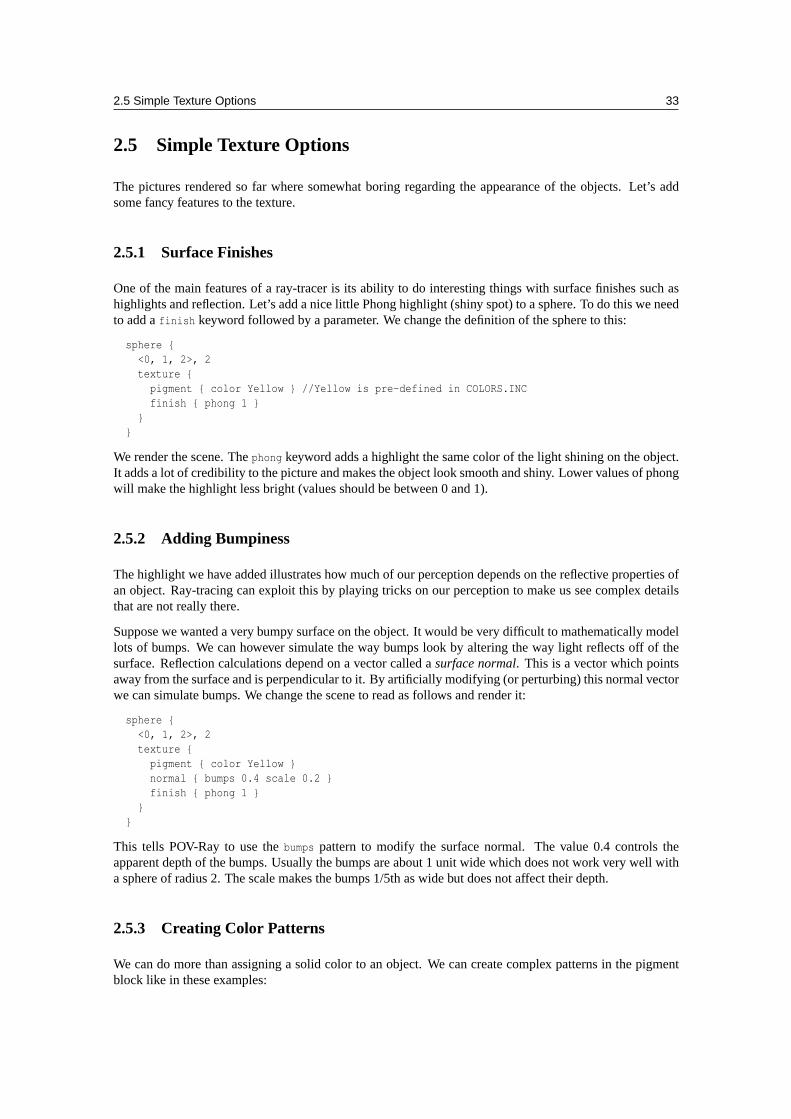
2.5 Simple Texture Options 33
2.5 Simple Texture Options
The pictures rendered so far where somewhat boring regarding the appearance of the objects. Let’s addsome fancy features to the texture.
2.5.1 Surface Finishes
One of the main features of a ray-tracer is its ability to do interesting things with surface finishes such ashighlights and reflection. Let’s add a nice little Phong highlight (shiny spot) to a sphere. To do this we needto add afinish keyword followed by a parameter. We change the definition of the sphere to this:
sphere {<0, 1, 2>, 2texture {
pigment { color Yellow } //Yellow is pre-defined in COLORS.INCfinish { phong 1 }
}}
We render the scene. Thephong keyword adds a highlight the same color of the light shining on the object.It adds a lot of credibility to the picture and makes the object look smooth and shiny. Lower values of phongwill make the highlight less bright (values should be between 0 and 1).
2.5.2 Adding Bumpiness
The highlight we have added illustrates how much of our perception depends on the reflective properties ofan object. Ray-tracing can exploit this by playing tricks on our perception to make us see complex detailsthat are not really there.
Suppose we wanted a very bumpy surface on the object. It would be very difficult to mathematically modellots of bumps. We can however simulate the way bumps look by altering the way light reflects off of thesurface. Reflection calculations depend on a vector called asurface normal. This is a vector which pointsaway from the surface and is perpendicular to it. By artificially modifying (or perturbing) this normal vectorwe can simulate bumps. We change the scene to read as follows and render it:
sphere {<0, 1, 2>, 2texture {
pigment { color Yellow }normal { bumps 0.4 scale 0.2 }finish { phong 1 }
}}
This tells POV-Ray to use thebumps pattern to modify the surface normal. The value 0.4 controls theapparent depth of the bumps. Usually the bumps are about 1 unit wide which does not work very well witha sphere of radius 2. The scale makes the bumps 1/5th as wide but does not affect their depth.
2.5.3 Creating Color Patterns
We can do more than assigning a solid color to an object. We can create complex patterns in the pigmentblock like in these examples:
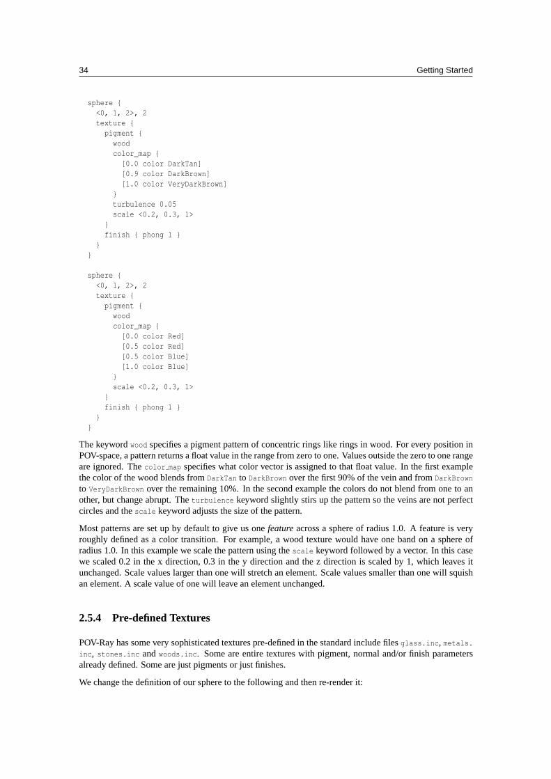
34 Getting Started
sphere {<0, 1, 2>, 2texture {
pigment {woodcolor_map {
[0.0 color DarkTan][0.9 color DarkBrown][1.0 color VeryDarkBrown]
}turbulence 0.05scale <0.2, 0.3, 1>
}finish { phong 1 }
}}
sphere {<0, 1, 2>, 2texture {
pigment {woodcolor_map {
[0.0 color Red][0.5 color Red][0.5 color Blue][1.0 color Blue]
}scale <0.2, 0.3, 1>
}finish { phong 1 }
}}
The keywordwood specifies a pigment pattern of concentric rings like rings in wood. For every position inPOV-space, a pattern returns a float value in the range from zero to one. Values outside the zero to one rangeare ignored. Thecolor map specifies what color vector is assigned to that float value. In the first examplethe color of the wood blends fromDarkTan to DarkBrown over the first 90% of the vein and fromDarkBrownto VeryDarkBrown over the remaining 10%. In the second example the colors do not blend from one to another, but change abrupt. Theturbulence keyword slightly stirs up the pattern so the veins are not perfectcircles and thescale keyword adjusts the size of the pattern.
Most patterns are set up by default to give us onefeatureacross a sphere of radius 1.0. A feature is veryroughly defined as a color transition. For example, a wood texture would have one band on a sphere ofradius 1.0. In this example we scale the pattern using thescale keyword followed by a vector. In this casewe scaled 0.2 in the x direction, 0.3 in the y direction and the z direction is scaled by 1, which leaves itunchanged. Scale values larger than one will stretch an element. Scale values smaller than one will squishan element. A scale value of one will leave an element unchanged.
2.5.4 Pre-defined Textures
POV-Ray has some very sophisticated textures pre-defined in the standard include filesglass.inc, metals.inc, stones.inc andwoods.inc. Some are entire textures with pigment, normal and/or finish parametersalready defined. Some are just pigments or just finishes.
We change the definition of our sphere to the following and then re-render it:
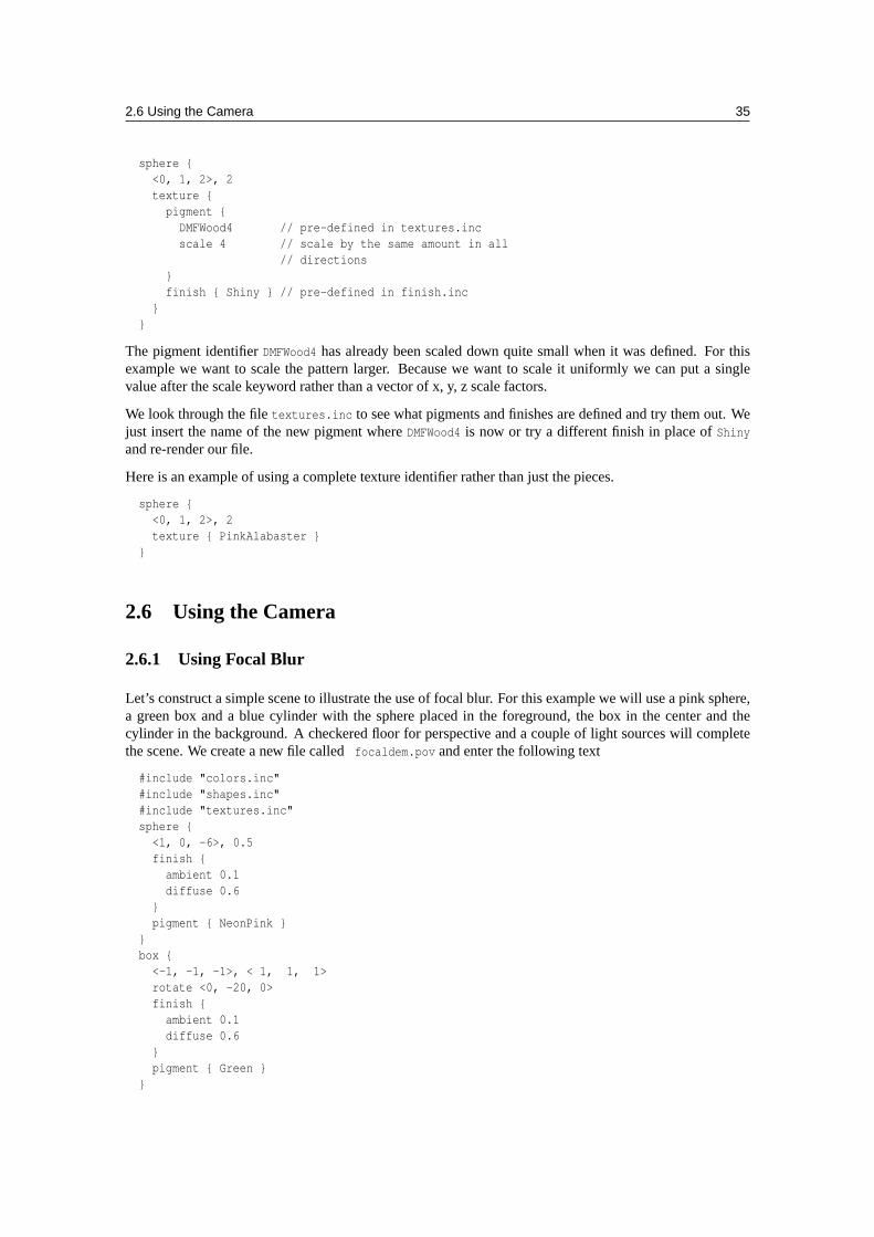
2.6 Using the Camera 35
sphere {<0, 1, 2>, 2texture {
pigment {DMFWood4 // pre-defined in textures.incscale 4 // scale by the same amount in all
// directions}finish { Shiny } // pre-defined in finish.inc
}}
The pigment identifierDMFWood4 has already been scaled down quite small when it was defined. For thisexample we want to scale the pattern larger. Because we want to scale it uniformly we can put a singlevalue after the scale keyword rather than a vector of x, y, z scale factors.
We look through the filetextures.inc to see what pigments and finishes are defined and try them out. Wejust insert the name of the new pigment whereDMFWood4 is now or try a different finish in place ofShinyand re-render our file.
Here is an example of using a complete texture identifier rather than just the pieces.
sphere {<0, 1, 2>, 2texture { PinkAlabaster }
}
2.6 Using the Camera
2.6.1 Using Focal Blur
Let’s construct a simple scene to illustrate the use of focal blur. For this example we will use a pink sphere,a green box and a blue cylinder with the sphere placed in the foreground, the box in the center and thecylinder in the background. A checkered floor for perspective and a couple of light sources will completethe scene. We create a new file calledfocaldem.pov and enter the following text
#include "colors.inc"#include "shapes.inc"#include "textures.inc"sphere {
<1, 0, -6>, 0.5finish {
ambient 0.1diffuse 0.6
}pigment { NeonPink }
}box {
<-1, -1, -1>, < 1, 1, 1>rotate <0, -20, 0>finish {
ambient 0.1diffuse 0.6
}pigment { Green }
}
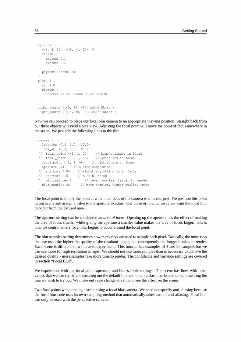
36 Getting Started
cylinder {<-6, 6, 30>, <-6, -1, 30>, 3finish {
ambient 0.1diffuse 0.6
}pigment {NeonBlue}
}plane {
y, -1.0pigment {
checker color Gray65 color Gray30}
}light_source { <5, 30, -30> color White }light_source { <-5, 30, -30> color White }
Now we can proceed to place our focal blur camera to an appropriate viewing position. Straight back fromour three objects will yield a nice view. Adjusting the focal point will move the point of focus anywhere inthe scene. We just add the following lines to the file:
camera {location <0.0, 1.0, -10.0>look_at <0.0, 1.0, 0.0>
// focal_point <-6, 1, 30> // blue cylinder in focus// focal_point < 0, 1, 0> // green box in focus
focal_point < 1, 1, -6> // pink sphere in focusaperture 0.4 // a nice compromise
// aperture 0.05 // almost everything is in focus// aperture 1.5 // much blurring// blur_samples 4 // fewer samples, faster to render
blur_samples 20 // more samples, higher quality image}
The focal point is simply the point at which the focus of the camera is at its sharpest. We position this pointin our scene and assign a value to the aperture to adjust how close or how far away we want the focal blurto occur from the focused area.
The aperture setting can be considered anarea of focus. Opening up the aperture has the effect of makingthe area of focus smaller while giving the aperture a smaller value makes the area of focus larger. This ishow we control where focal blur begins to occur around the focal point.
The blur samples setting determines how many rays are used to sample each pixel. Basically, the more raysthat are used the higher the quality of the resultant image, but consequently the longer it takes to render.Each scene is different so we have to experiment. This tutorial has examples of 4 and 20 samples but wecan use more for high resolution images. We should not use more samples than is necessary to achieve thedesired quality - more samples take more time to render. The confidence and variance settings are coveredin section “Focal Blur”.
We experiment with the focal point, aperture, and blur sample settings. The scene has lines with othervalues that we can try by commenting out the default line with double slash marks and un-commenting theline we wish to try out. We make only one change at a time to see the effect on the scene.
Two final points when tracing a scene using a focal blur camera. We need not specify anti-aliasing becausethe focal blur code uses its own sampling method that automatically takes care of anti-aliasing. Focal blurcan only be used with the perspective camera.
2.7 POV-Ray Coordinate System 37
2.7 POV-Ray Coordinate System
Objects, lights and the camera are positioned using a typical 3D coordinate system. The usual coordinatesystem for POV-Ray has the positive y-axis pointing up, the positive x-axis pointing to the right and thepositive z-axis pointing into the screen. The negative values of the axes point the other direction as shownin the images in section “Understanding POV-Ray’s Coordinate System”.
Locations within that coordinate system are usually specified by a three component vector. The three valuescorrespond to the x, y and z directions respectively. For example, the vector<1,2,3> means the point thatis one unit to the right, two units up and three units in front of the center of the universe at<0,0,0>.
Vectors are not always points though. They can also refer to an amount to size, move or rotate a sceneelement or to modify the texture pattern applied to an object.
The size, location, orientation, and deformation of items within the coordinate system is controlled bymodifiers calledtransformations. The follow sub-sections describe the transformations and their usage.
2.7.1 Transformations
The supported transformations arerotate, scale, andtranslate. They are used to turn, size and move anobject or texture. A transformation matrix may also be used to specify complex transformations directly.Groups of transformations may be merged together and stored in a transformation identifier. The syntax fortransformations is as follows.
TRANSFORMATION:rotate <Rotate_Amt> | scale <Scale_Amt> |translate <Translate_Amt> | transform TRANSFORM_IDENTIFIER |transform { TRANSFORMATION_BLOCK...} |matrix <Val00, Val01, Val02,
Val10, Val11, Val12,Val20, Val21, Val22,Val30, Val31, Val32>
TRANSFORMATION_BLOCK:TRANSFORM_IDENTIFIER | TRANSFORMATION | inverse
TRANSFORM_DECLARATION:#declare IDENTIFIER = transform { TRANSFORMATION_BLOCK...} |#local IDENTIFIER = transform { TRANSFORMATION_BLOCK...}
Translate
Items may be moved by adding atranslate modifier. It consists of the keywordtranslate followed by avector expression. The three terms of the vector specify the number of units to move in each of the x, y andz directions. Translate moves the element relative to its current position. For example
sphere { <10, 10, 10>, 1pigment { Green }translate <-5, 2, 1>
}
will move the sphere from the location<10,10,10> to <5,12,11>. It does not move it to the absolutelocation<-5,2,1>. Translations are always relative to the item’s location before the move. Translating byzero will leave the element unchanged on that axis. For example:
sphere { <10, 10, 10>, 1pigment { Green }translate 3*x // evaluates to <3,0,0> so move 3 units
38 Getting Started
// in the x direction and none along y or z}
Scale
You may change the size of an object or texture pattern by adding ascale modifier. It consists of thekeywordscale followed by a vector expression. The three terms of the vector specify the amount of scalingin each of the x, y and z directions.
Uneven scaling is used tostretchor squishan element. Values larger than one stretch the element on thataxis while values smaller than one are used to squish it. Scale is relative to the current element size. If theelement has been previously re-sized using scale then scale will size relative to the new size. Multiple scalevalues may used.
For example
sphere { <0,0,0>, 1scale <2,1,0.5>
}
will stretch and smash the sphere into an ellipsoid shape that is twice the original size along the x-direction,remains the same size in the y-direction and is half the original size in the z-direction.
If a lone float expression is specified it is promoted to a three component vector whose terms are all thesame. Thus the item is uniformly scaled by the same amount in all directions. For example:
object {MyObjectscale 5 // Evaluates as <5,5,5> so uniformly scale
// by 5 in every direction.}
When one of the scaling components is zero, POV-Ray changes this component to 1 since it assumes that 0means no scaling in this direction. A warning “Illegal Value: Scale X, Y or Z by 0.0. Changed to 1.0.” isprinted then.
Rotate
You may change the orientation of an object or texture pattern by adding arotate modifier. It consists ofthe keyword rotate followed by a vector expression. The three terms of the vector specify the number ofdegrees to rotate about each of the x-, y- and z-axes.
Note: that the order of the rotations does matter. Rotations occur about the x-axis first, then the y-axis, thenthe z-axis. If you are not sure if this is what you want then you should only rotate on one axis at a timeusing multiple rotation statements to get a correct rotation.
rotate <0, 30, 0> // 30 degrees around Y axis then,rotate <-20, 0, 0> // -20 degrees around X axis then,rotate <0, 0, 10> // 10 degrees around Z axis.
Rotation is always performed relative to the axis. Thus if an object is some distance from the axis of rotationit will not only rotate but it willorbit about the axis as though it was swinging around on an invisible string.
POV-Ray uses a left-handed rotation system. Using the famous “Computer Graphics Aerobics” exercise,you hold up your left hand and point your thumb in the positive direction of the axis of rotation. Your fingerswill curl in the positive direction of rotation. Similarly if you point your thumb in the negative directionof the axis your fingers will curl in the negative direction of rotation. See “Understanding POV-Ray’sCoordinate System” for an illustration.
2.7 POV-Ray Coordinate System 39
Matrix
The matrix keyword can be used to explicitly specify the transformation matrix to be used for objects ortextures. Its syntax is:
MATRIX:matrix <Val00, Val01, Val02,
Val10, Val11, Val12,Val20, Val21, Val22,Val30, Val31, Val32>
WhereVal00 throughVal32 are float expressions enclosed in angle brackets and separated by commas.
Note: this is not a vector. It is a set of 12 float expressions.
These floats specify the elements of a 4 by 4 matrix with the fourth column implicitly set to<0,0,0,1>. Atany given pointP, P=<px, py, pz>, is transformed into the pointQ, Q=<qx, qy, qz> by
qx = Val00 * px + Val10 * py + Val20 * pz + Val30
qy = Val01 * px + Val11 * py + Val21 * pz + Val31
qz = Val02 * px + Val12 * py + Val22 * pz + Val32
Normally you will not use the matrix keyword because it is less descriptive than the transformation com-mands and harder to visualize. However the matrix command allows more general transformation effectslike shearing. The following matrix causes an object to be sheared along the y-axis.
object {MyObjectmatrix < 1, 1, 0,
0, 1, 0,0, 0, 1,0, 0, 0 >
}
2.7.2 Transformation Order
Because rotations are always relative to the axis and scaling is relative to the origin, you will generallywant to create an object at the origin and scale and rotate it first. Then you may translate it into its properposition. It is a common mistake to carefully position an object and then to decide to rotate it. Howeverbecause a rotation of an object causes it to orbit about the axis, the position of the object may change somuch that it orbits out of the field of view of the camera!
Similarly scaling after translation also moves an object unexpectedly. If you scale after you translate thescale will multiply the translate amount.For example
translate <5, 6, 7>scale 4
will translate to<20,24,28> instead of <5,6,7>. Be careful when transforming to get the order correctfor your purposes.
2.7.3 Inverse Transform
transform { scale <20,24,28> translate y*3 inverse }
40 Getting Started
An inverse transform does the opposite of what the transform would normally do, and can be used to“undo” transforms without messing around with huge numbers of transformations. To do the same withoutthis inverse, you would have to duplicate each transform, change them to do the opposite of what theywould normally do (for exampletranslate -y*3 instead oftranslate y*3)and reverse their order.
2.7.4 Transform Identifiers
At times it is useful to combine together several transformations and apply them in multiple places. Atransform identifier may be used for this purpose. Transform identifiers are declared as follows:
TRANSFORM_DECLARATION:#declare IDENTIFIER = transform{ TRANSFORMATION... } |#local IDENTIFIER = transform{ TRANSFORMATION... }
WhereIDENTIFIER is the name of the identifier up to 40 characters long andTRANSFORMATIONis anyvalid transformation modifier. See “#declare vs. #local” for information on identifier scope. Here is anexample...
#declare MyTrans =transform {
rotate THISWAYscale SOMUCHrotate -THISWAYscale BIGGERtranslate OVERTHERErotate WAYAROUND
}
A transform identifier is invoked by thetransform keyword with or without brackets as shown here:
object {MyObject // Get a copy of MyObjecttransform MyTrans // Apply the transformationtranslate -x*5 // Then move it 5 units left
}object {
MyObject // Get another copy of MyObjecttransform { MyTrans } // Apply the same transformationtranslate x*5 // Then move this one 5 units right
}
On extremely complex CSG objects with lots of components it may speed up parsing if you apply a declaredtransformation rather than the individualtranslate, rotate, scale, or matrix modifiers. Thetransformis attached just once to each component. Applying each individualtranslate, rotate, scale, or matrixmodifiers takes longer. This only affects parsing - rendering works the same either way.
2.7.5 Transforming Textures and Objects
When an object is transformed all textures attached to the objectat that timeare transformed as well. Thismeans that if you have atranslate, rotate, scale, or matrix modifier in an objectbeforea texture,then the texture will not be transformed. If the transformation isafter the texture then the texture will betransformed with the object. If the transformation isinsidethetexture statement thenonly the textureisaffected. The shape remains the same. For example:
sphere { 0, 1texture { Jade } // texture identifier from TEXTURES.INCscale 3 // this scale affects both the
2.8 Setting POV-Ray Options 41
// shape and texture}sphere { 0, 1scale 3 // this scale affects the shape onlytexture { Jade }
}sphere { 0, 1texture {Jadescale 3 // this scale affects the texture only
}}
Transformations may also be independently applied to pigment patterns and surface normal patterns.
Note: scaling a normal pattern not only affects the width and spacing. It does also affect the apparent heightor depth of the bumps, for how to avoid this see Scaling normals.
For example:
box { <0, 0, 0>, <1, 1, 1>texture {pigment {checker Red, Whitescale 0.25 // This affects only the color pattern
}normal {bumps 0.3 // This specifies apparent height of bumpsscale 0.2 // Scales diameter and space between bumps
// and also the height. Has no effect on// color pattern.
}rotate y*45 // This affects the entire texture but
} // not the object.}
2.8 Setting POV-Ray Options
POV-Ray was originally created as a command-line program for operating systems without graphical inter-faces, dialog boxes and pull-down menus. Most versions of POV-Ray still use command-line switches totell it what to do. This documentation assumes you are using the command-line version. If you are usingMacintosh, MS-Windows or other GUI versions, there will be dialog boxes or menus which do the samething. There is system-specific documentation for each system describing the specific commands.
There are two distinct ways of setting POV-Ray options (other than through the GUI interface, if applicable): command line switches and INI file keywords. Both are explained in detail in the following sections.
2.8.1 Command Line Switches
Command line switches consist of a+ (plus) or - (minus) sign, followed by one or more alphabeticcharacters and possibly a numeric value. Here is a typical command line with switches.
POVRAY +Isimple.pov +V +W80 +H60
povray is the name of the program and it is followed by several switches. Each switch begins with a plusor minus sign. The+I switch with the filename tells POV-Ray what scene file it should use as input and
42 Getting Started
+V tells the program to output its status to the text screen as it is working. The+W and +H switches set thewidth and height of the image in pixels. This image will be 80 pixels wide by 60 pixels high.
In switches which toggle a feature, the plus turns it on and minus turns it off. For example+P turns on thepause for keypress when finishedoption while-P turns it off. Other switches are used to specify values anddo not toggle a feature. Either plus or minus may be used in that instance. For example+W320 sets the widthto 320 pixels. You could also use-W320 and get the same results.
Switches may be specified in upper or lower case. They are read left to right but in general may be specifiedin any order. If you specify a switch more than once, the previous value is generally overwritten with thelast specification. The only exception is the+L switch for setting library paths. Up to ten unique paths maybe specified.
Almost all + or - switches have an equivalent option which can be used in an INI file which is describedin the next section. A detailed description of each switch is given in the option reference section.
2.8.2 Using INI Files
Note: although the term ’INI file’ is used by POV-Ray, this was implemented before the widespreadacceptance of Microsoft Windows, and while POV-Ray’s INI files are almost identical to those of Windows,there are some minor differences (the foremost being that it is legal to have multiple instances of the sameitem in a section). INI files are used on all platform versions of POV-Ray, not just on the Windows platform.
Because it is difficult to set more than a few options on a command line, you have the ability to put multipleoptions in one or more text files. These initialization files or INI files have .ini as their default extension.Previous versions of POV-Ray called them default files or DEF files. You may still use existing DEF fileswith this version of POV-Ray.
The majority of options you use will be stored in INI files. The command line switches are recommendedfor options which you will turn off or on frequently as you perform test renderings of a scene you aredeveloping. The file povray.ini is automatically read if present. You may specify additional INI files onthe command-line by simply typing the file name on the command line. For example:
POVRAY MYOPTS.INI
If no extension is given, then.ini is assumed. POV-Ray knows this is not a switch because it is not precededby a plus or minus.
You may have multiple INI files on the command line along with switches. For example:
POVRAY MYOPTS +V OTHER
This reads options frommyopts.ini, then sets the+V switch, then reads options fromother.ini.
An INI file is a plain ASCII text file with options of the form...
Option_keyword=VALUE ; Text after semicolon is a comment
For example the INI equivalent of the switch+Isimple.pov is...
Input_File_Name=simple.pov
Options are read top to bottom in the file but in general may be specified in any order. If you specify anoption more than once, the previous values are generally overwritten with the last specification. The onlyexception is theLibrary Path=path options. Up to 25 unique paths may be specified.
Almost all INI-style options have equivalent+ or - switches. The option reference section gives a detaileddescription of all POV-Ray options. It includes both the INI-style settings and the+/- switches.
The INI keywords are not case sensitive. Only one INI option is permitted per line of text. You may alsoinclude switches in your INI file if they are easier for you. You may have multiple switches per line but you
2.8 Setting POV-Ray Options 43
should not mix switches and INI options on the same line. You may nest INI files by simply putting the filename on a line by itself with no equals sign after it. Nesting may occur up to ten levels deep. For example:
; This is a sample INI file. This entire line is a comment.; Blank lines are permitted.Input_File_Name=simple.pov ;This sets the input file name+W80 +H60 ; Traditional +/- switches are permitted tooMOREOPT ; Read MOREOPT.INI and continue with next line+V ; Another switch; That’s all folks!
INI files may have labeled sections so that more than one set of options may be stored in a single file. Eachsection begins with a label in [] brackets. For example:
; RES.INI; This sample INI file is used to set resolution.+W120 +H100 ; This section has no label.
; Select it with "RES"[Low]+W80 +H60 ; This section has a label.
; Select it with "RES[Low]"[Med]+W320 +H200 ; This section has a label.
; Select it with "RES[Med]"[High]+W640 +H480 ; Labels are not case sensitive.
; "RES[high]" works[Really High]+W800 +H600 ; Labels may contain blanks
When you specify the INI file you should follow it with the section label in brackets. For example...
POVRAY RES[Med] +Imyfile.pov
POV-Ray readsres.ini and skips all options until it finds the labelMed. It processes options after that labeluntil it finds another label and then it skips. If no label is specified on the command line then only theunlabeled area at the top of the file is read. If a label is specified, the unlabeled area is ignored.
If a file or path contains blanks the whole file and path specification has to be put in quotes. You may eitheruse a double-quote oir a single-quote, but you have to use the same at the beginning and end. For example:
+I"my file.pov"+I’my file.pov’Input_File="my file.pov"Input_File=’my file.pov’
By using either single or double quotes it is possible to specify files whose name or path contains either aspart of the name. For example:
+I"file’s.pov"+I’my "big" file.pov’Input_File="file’s.pov"Input_File=’my "big" file.pov’
2.8.3 Using the POVINI Environment Variable
The environment variable POVINI is used to specify the location and name of a default INI file that isread every time POV-Ray is executed. If POVINI is not specified, or if your computer platform does notuse environment variables, a default INI file may be read. If the specified file does not exist, a warning

44 Getting Started
message is printed. To set the environment variable under MS-DOS you might put the following line inyourautoexec.bat file...
set POVINI=c:\povray3\default.ini
On most operating systems the sequence of reading options is as follows:
1. Read options from default INI file specified by the POVINI environment variable or platform specificINI file.
2. Read switches from command line (this includes reading any specified INI/DEF files).
The POVRAYOPT environment variable supported by previous POV-Ray versions is no longer available.
Chapter 3
Advanced Features
3.1 Spline Based Shapes
After we have gained some experience with the simpler shapes available in POV-Ray it is time to go on tothe more advanced, thrilling shapes.
We should be aware that the shapes described in this and the following two chapters are not trivial tounderstand. We need not be worried though if we do not know how to use them or how they work. We justtry the examples and play with the features described in the reference chapter. There is nothing better thanlearning by doing.
You may wish to skip to the chapter “Simple Texture Options” before proceeding with these advancedshapes.
3.1.1 Lathe Object
In the real world,lathe refers to a process of making patterned rounded shapes by spinning the sourcematerial in place and carving pieces out as it turns. The results can be elaborate, smoothly rounded, elegantlooking artefacts such as table legs, pottery, etc. In POV-Ray, a lathe object is used for creating much thesame kind of items, although we are referring to the object itself rather than the means of production.
Here is some source for a really basic lathe.
#include "colors.inc"background{White}camera {
angle 10location <1, 9, -50>look_at <0, 2, 0>
}light_source {
<20, 20, -20> color White}lathe {
linear_spline6,<0,0>, <1,1>, <3,2>, <2,3>, <2,4>, <0,4>pigment { Blue }finish {
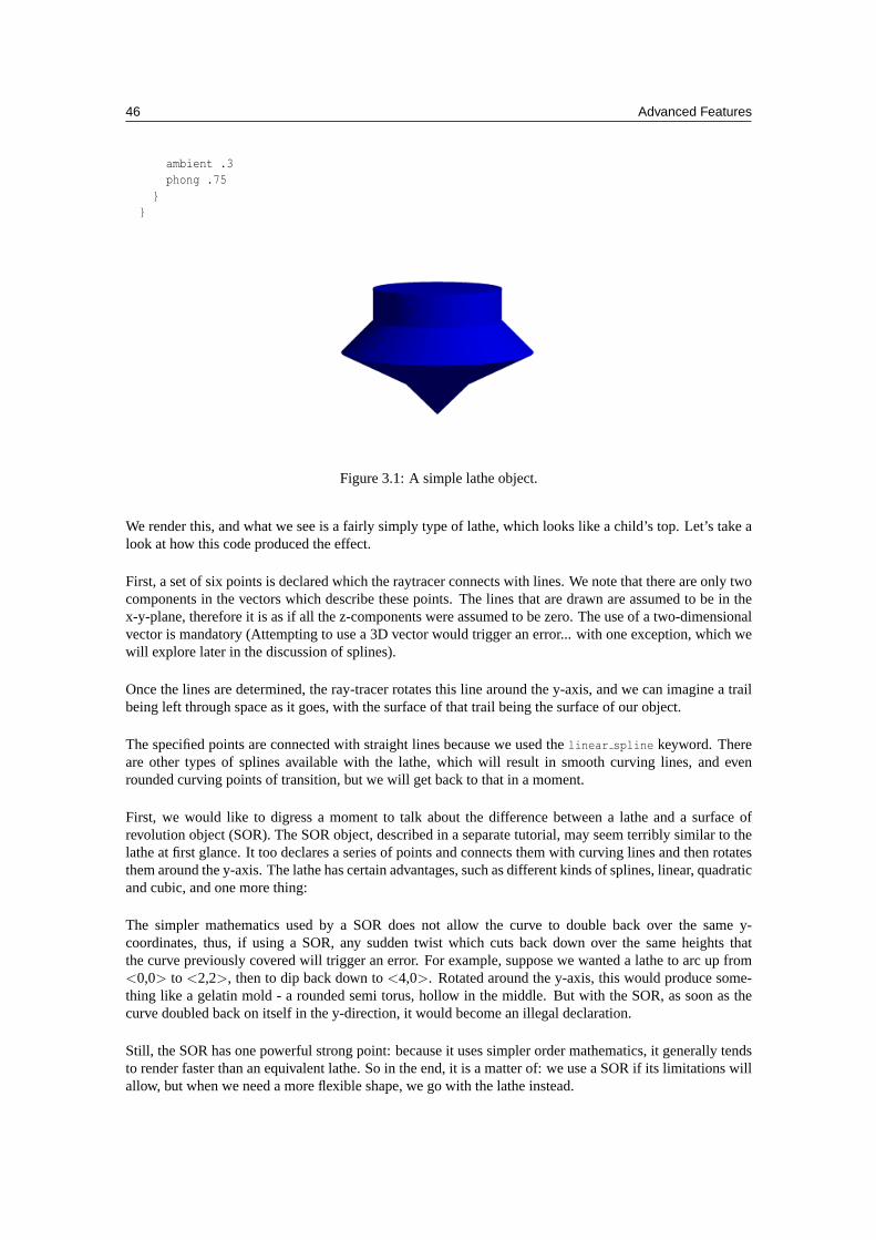
46 Advanced Features
ambient .3phong .75
}}
Figure 3.1: A simple lathe object.
We render this, and what we see is a fairly simply type of lathe, which looks like a child’s top. Let’s take alook at how this code produced the effect.
First, a set of six points is declared which the raytracer connects with lines. We note that there are only twocomponents in the vectors which describe these points. The lines that are drawn are assumed to be in thex-y-plane, therefore it is as if all the z-components were assumed to be zero. The use of a two-dimensionalvector is mandatory (Attempting to use a 3D vector would trigger an error... with one exception, which wewill explore later in the discussion of splines).
Once the lines are determined, the ray-tracer rotates this line around the y-axis, and we can imagine a trailbeing left through space as it goes, with the surface of that trail being the surface of our object.
The specified points are connected with straight lines because we used thelinear spline keyword. Thereare other types of splines available with the lathe, which will result in smooth curving lines, and evenrounded curving points of transition, but we will get back to that in a moment.
First, we would like to digress a moment to talk about the difference between a lathe and a surface ofrevolution object (SOR). The SOR object, described in a separate tutorial, may seem terribly similar to thelathe at first glance. It too declares a series of points and connects them with curving lines and then rotatesthem around the y-axis. The lathe has certain advantages, such as different kinds of splines, linear, quadraticand cubic, and one more thing:
The simpler mathematics used by a SOR does not allow the curve to double back over the same y-coordinates, thus, if using a SOR, any sudden twist which cuts back down over the same heights thatthe curve previously covered will trigger an error. For example, suppose we wanted a lathe to arc up from<0,0> to <2,2>, then to dip back down to<4,0>. Rotated around the y-axis, this would produce some-thing like a gelatin mold - a rounded semi torus, hollow in the middle. But with the SOR, as soon as thecurve doubled back on itself in the y-direction, it would become an illegal declaration.
Still, the SOR has one powerful strong point: because it uses simpler order mathematics, it generally tendsto render faster than an equivalent lathe. So in the end, it is a matter of: we use a SOR if its limitations willallow, but when we need a more flexible shape, we go with the lathe instead.
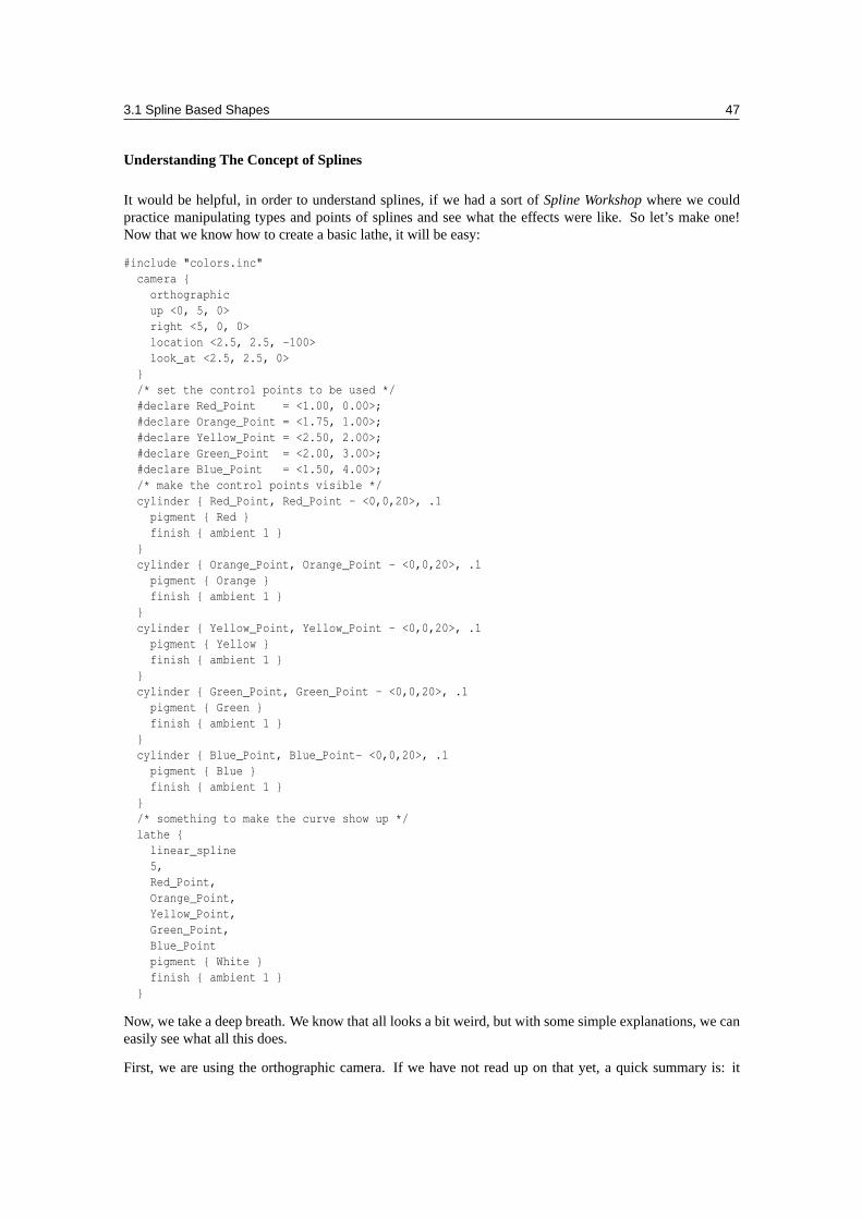
3.1 Spline Based Shapes 47
Understanding The Concept of Splines
It would be helpful, in order to understand splines, if we had a sort ofSpline Workshopwhere we couldpractice manipulating types and points of splines and see what the effects were like. So let’s make one!Now that we know how to create a basic lathe, it will be easy:
#include "colors.inc"camera {
orthographicup <0, 5, 0>right <5, 0, 0>location <2.5, 2.5, -100>look_at <2.5, 2.5, 0>
}/* set the control points to be used */#declare Red_Point = <1.00, 0.00>;#declare Orange_Point = <1.75, 1.00>;#declare Yellow_Point = <2.50, 2.00>;#declare Green_Point = <2.00, 3.00>;#declare Blue_Point = <1.50, 4.00>;/* make the control points visible */cylinder { Red_Point, Red_Point - <0,0,20>, .1
pigment { Red }finish { ambient 1 }
}cylinder { Orange_Point, Orange_Point - <0,0,20>, .1
pigment { Orange }finish { ambient 1 }
}cylinder { Yellow_Point, Yellow_Point - <0,0,20>, .1
pigment { Yellow }finish { ambient 1 }
}cylinder { Green_Point, Green_Point - <0,0,20>, .1
pigment { Green }finish { ambient 1 }
}cylinder { Blue_Point, Blue_Point- <0,0,20>, .1
pigment { Blue }finish { ambient 1 }
}/* something to make the curve show up */lathe {
linear_spline5,Red_Point,Orange_Point,Yellow_Point,Green_Point,Blue_Pointpigment { White }finish { ambient 1 }
}
Now, we take a deep breath. We know that all looks a bit weird, but with some simple explanations, we caneasily see what all this does.
First, we are using the orthographic camera. If we have not read up on that yet, a quick summary is: it
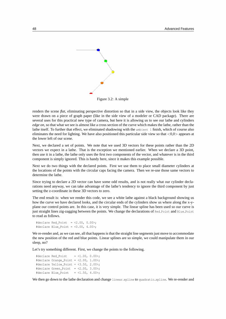
48 Advanced Features
Figure 3.2: A simple
renders the sceneflat, eliminating perspective distortion so that in a side view, the objects look like theywere drawn on a piece of graph paper (like in the side view of a modeler or CAD package). There areseveral uses for this practical new type of camera, but here it is allowing us to see our lathe and cylindersedge on, so that what we see is almost like a cross section of the curve which makes the lathe, rather than thelathe itself. To further that effect, we eliminated shadowing with theambient 1 finish, which of course alsoeliminates the need for lighting. We have also positioned this particular side view so that<0,0> appears atthe lower left of our scene.
Next, we declared a set of points. We note that we used 3D vectors for these points rather than the 2Dvectors we expect in a lathe. That is the exception we mentioned earlier. When we declare a 3D point,then use it in a lathe, the lathe only uses the first two components of the vector, and whatever is in the thirdcomponent is simply ignored. This is handy here, since it makes this example possible.
Next we do two things with the declared points. First we use them to place small diameter cylinders atthe locations of the points with the circular caps facing the camera. Then we re-use those same vectors todetermine the lathe.
Since trying to declare a 2D vector can have some odd results, and is not really what our cylinder decla-rations need anyway, we can take advantage of the lathe’s tendency to ignore the third component by justsetting the z-coordinate in these 3D vectors to zero.
The end result is: when we render this code, we see a white lathe against a black background showing ushow the curve we have declared looks, and the circular ends of the cylinders show us where along the x-y-plane our control points are. In this case, it is very simple. The linear spline has been used so our curve isjust straight lines zig-zagging between the points. We change the declarations ofRed Point andBlue Point
to read as follows.
#declare Red_Point = <2.00, 0.00>;#declare Blue_Point = <0.00, 4.00>;
We re-render and, as we can see, all that happens is that the straight line segments just move to accommodatethe new position of the red and blue points. Linear splines are so simple, we could manipulate them in oursleep, no?
Let’s try something different. First, we change the points to the following.
#declare Red_Point = <1.00, 0.00>;#declare Orange_Point = <2.00, 1.00>;#declare Yellow_Point = <3.50, 2.00>;#declare Green_Point = <2.00, 3.00>;#declare Blue_Point = <1.50, 4.00>;
We then go down to the lathe declaration and changelinear spline to quadratic spline. We re-render and
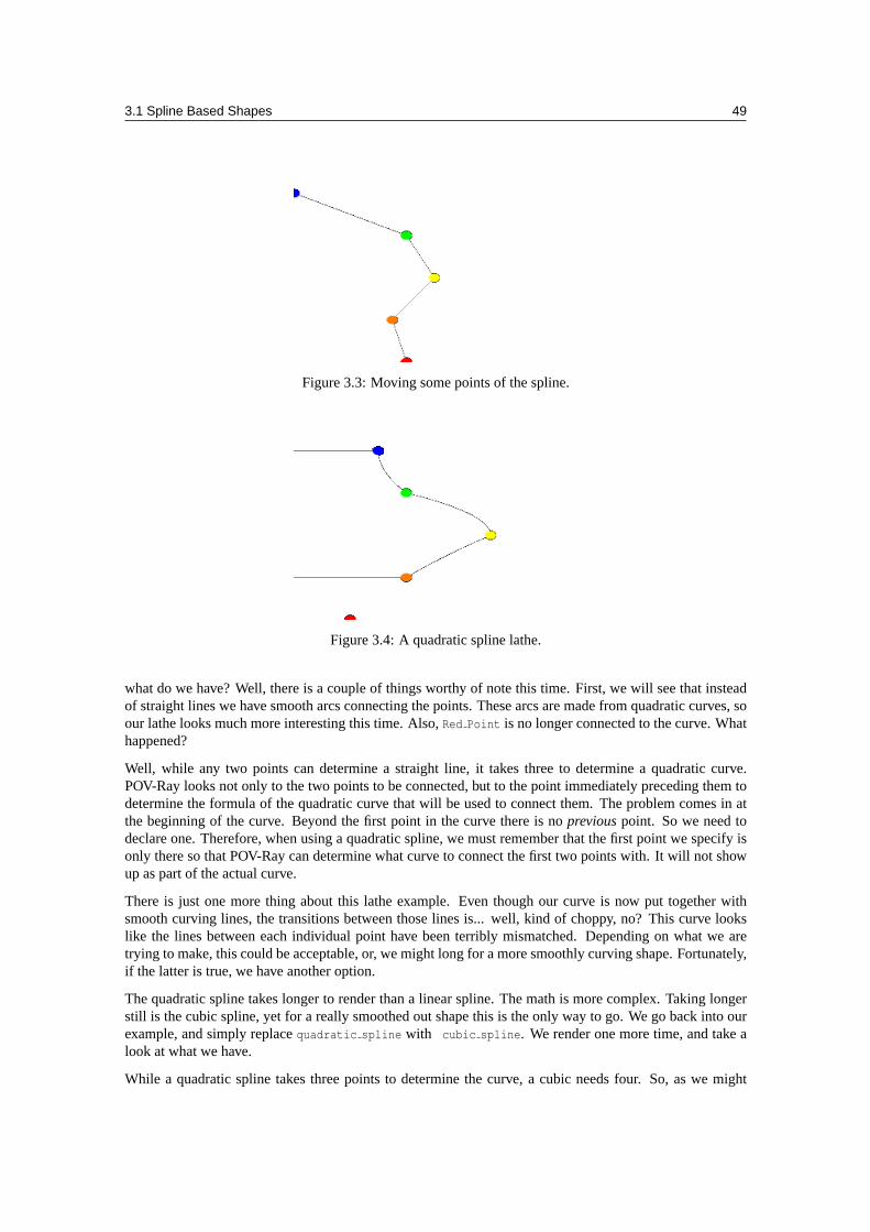
3.1 Spline Based Shapes 49
Figure 3.3: Moving some points of the spline.
Figure 3.4: A quadratic spline lathe.
what do we have? Well, there is a couple of things worthy of note this time. First, we will see that insteadof straight lines we have smooth arcs connecting the points. These arcs are made from quadratic curves, soour lathe looks much more interesting this time. Also,Red Point is no longer connected to the curve. Whathappened?
Well, while any two points can determine a straight line, it takes three to determine a quadratic curve.POV-Ray looks not only to the two points to be connected, but to the point immediately preceding them todetermine the formula of the quadratic curve that will be used to connect them. The problem comes in atthe beginning of the curve. Beyond the first point in the curve there is nopreviouspoint. So we need todeclare one. Therefore, when using a quadratic spline, we must remember that the first point we specify isonly there so that POV-Ray can determine what curve to connect the first two points with. It will not showup as part of the actual curve.
There is just one more thing about this lathe example. Even though our curve is now put together withsmooth curving lines, the transitions between those lines is... well, kind of choppy, no? This curve lookslike the lines between each individual point have been terribly mismatched. Depending on what we aretrying to make, this could be acceptable, or, we might long for a more smoothly curving shape. Fortunately,if the latter is true, we have another option.
The quadratic spline takes longer to render than a linear spline. The math is more complex. Taking longerstill is the cubic spline, yet for a really smoothed out shape this is the only way to go. We go back into ourexample, and simply replacequadratic spline with cubic spline. We render one more time, and take alook at what we have.
While a quadratic spline takes three points to determine the curve, a cubic needs four. So, as we might
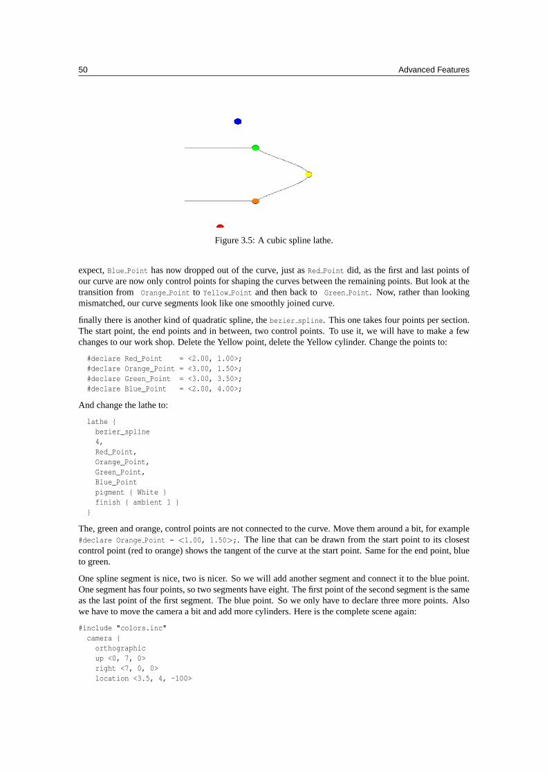
50 Advanced Features
Figure 3.5: A cubic spline lathe.
expect,Blue Point has now dropped out of the curve, just asRed Point did, as the first and last points ofour curve are now only control points for shaping the curves between the remaining points. But look at thetransition from Orange Point to Yellow Point and then back toGreen Point. Now, rather than lookingmismatched, our curve segments look like one smoothly joined curve.
finally there is another kind of quadratic spline, thebezier spline. This one takes four points per section.The start point, the end points and in between, two control points. To use it, we will have to make a fewchanges to our work shop. Delete the Yellow point, delete the Yellow cylinder. Change the points to:
#declare Red_Point = <2.00, 1.00>;#declare Orange_Point = <3.00, 1.50>;#declare Green_Point = <3.00, 3.50>;#declare Blue_Point = <2.00, 4.00>;
And change the lathe to:
lathe {bezier_spline4,Red_Point,Orange_Point,Green_Point,Blue_Pointpigment { White }finish { ambient 1 }
}
The, green and orange, control points are not connected to the curve. Move them around a bit, for example#declare Orange Point = <1.00, 1.50>;. The line that can be drawn from the start point to its closestcontrol point (red to orange) shows the tangent of the curve at the start point. Same for the end point, blueto green.
One spline segment is nice, two is nicer. So we will add another segment and connect it to the blue point.One segment has four points, so two segments have eight. The first point of the second segment is the sameas the last point of the first segment. The blue point. So we only have to declare three more points. Alsowe have to move the camera a bit and add more cylinders. Here is the complete scene again:
#include "colors.inc"camera {
orthographicup <0, 7, 0>right <7, 0, 0>location <3.5, 4, -100>
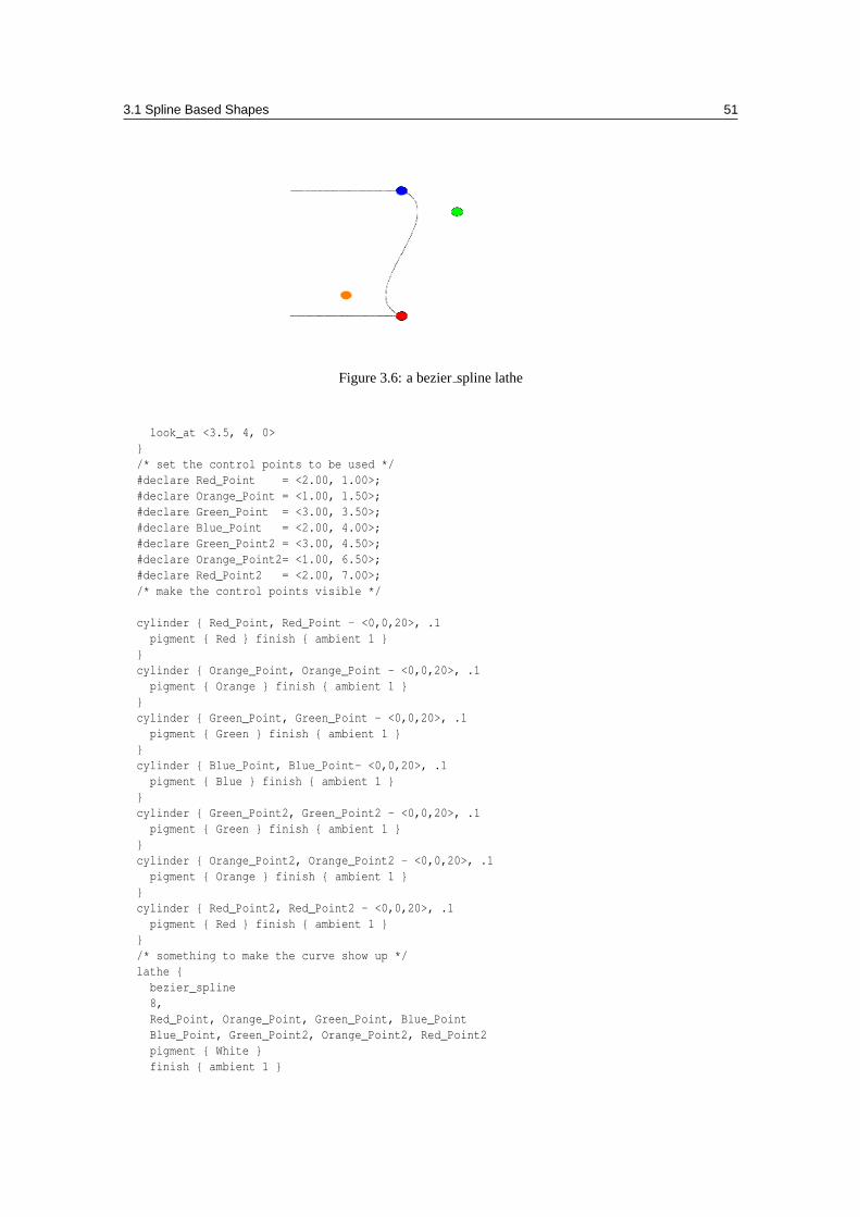
3.1 Spline Based Shapes 51
Figure 3.6: a bezierspline lathe
look_at <3.5, 4, 0>}/* set the control points to be used */#declare Red_Point = <2.00, 1.00>;#declare Orange_Point = <1.00, 1.50>;#declare Green_Point = <3.00, 3.50>;#declare Blue_Point = <2.00, 4.00>;#declare Green_Point2 = <3.00, 4.50>;#declare Orange_Point2= <1.00, 6.50>;#declare Red_Point2 = <2.00, 7.00>;/* make the control points visible */
cylinder { Red_Point, Red_Point - <0,0,20>, .1pigment { Red } finish { ambient 1 }
}cylinder { Orange_Point, Orange_Point - <0,0,20>, .1
pigment { Orange } finish { ambient 1 }}cylinder { Green_Point, Green_Point - <0,0,20>, .1
pigment { Green } finish { ambient 1 }}cylinder { Blue_Point, Blue_Point- <0,0,20>, .1
pigment { Blue } finish { ambient 1 }}cylinder { Green_Point2, Green_Point2 - <0,0,20>, .1
pigment { Green } finish { ambient 1 }}cylinder { Orange_Point2, Orange_Point2 - <0,0,20>, .1
pigment { Orange } finish { ambient 1 }}cylinder { Red_Point2, Red_Point2 - <0,0,20>, .1
pigment { Red } finish { ambient 1 }}/* something to make the curve show up */lathe {
bezier_spline8,Red_Point, Orange_Point, Green_Point, Blue_PointBlue_Point, Green_Point2, Orange_Point2, Red_Point2pigment { White }finish { ambient 1 }
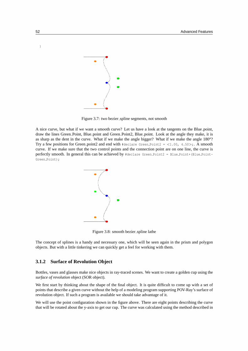
52 Advanced Features
}
Figure 3.7: two bezierspline segments, not smooth
A nice curve, but what if we want a smooth curve? Let us have a look at the tangents on the Bluepoint,draw the lines GreenPoint, Bluepoint and GreenPoint2, Bluepoint. Look at the angle they make, it isas sharp as the dent in the curve. What if we make the angle bigger? What if we make the angle 180°?Try a few positions for Greenpoint2 and end with#declare Green Point2 = <1.00, 4.50>;. A smoothcurve. If we make sure that the two control points and the connection point are on one line, the curve isperfectly smooth. In general this can be achieved by#declare Green Point2 = Blue Point+(Blue Point-
Green Point);
Figure 3.8: smooth bezierspline lathe
The concept of splines is a handy and necessary one, which will be seen again in the prism and polygonobjects. But with a little tinkering we can quickly get a feel for working with them.
3.1.2 Surface of Revolution Object
Bottles, vases and glasses make nice objects in ray-traced scenes. We want to create a golden cup using thesurface of revolutionobject (SOR object).
We first start by thinking about the shape of the final object. It is quite difficult to come up with a set ofpoints that describe a given curve without the help of a modeling program supporting POV-Ray’s surface ofrevolution object. If such a program is available we should take advantage of it.
We will use the point configuration shown in the figure above. There are eight points describing the curvethat will be rotated about the y-axis to get our cup. The curve was calculated using the method described in
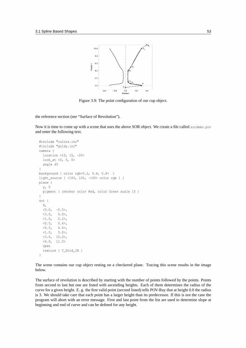
3.1 Spline Based Shapes 53
Figure 3.9: The point configuration of our cup object.
the reference section (see “Surface of Revolution”).
Now it is time to come up with a scene that uses the above SOR object. We create a file calledsordemo.pov
and enter the following text.
#include "colors.inc"#include "golds.inc"camera {
location <10, 15, -20>look_at <0, 5, 0>angle 45
}background { color rgb<0.2, 0.4, 0.8> }light_source { <100, 100, -100> color rgb 1 }plane {
y, 0pigment { checker color Red, color Green scale 10 }
}sor {
8,<0.0, -0.5>,<3.0, 0.0>,<1.0, 0.2>,<0.5, 0.4>,<0.5, 4.0>,<1.0, 5.0>,<3.0, 10.0>,<4.0, 11.0>opentexture { T_Gold_1B }
}
The scene contains our cup object resting on a checkered plane. Tracing this scene results in the imagebelow.
The surface of revolution is described by starting with the number of points followed by the points. Pointsfrom second to last but one are listed with ascending heights. Each of them determines the radius of thecurve for a given height. E. g. the first valid point (second listed) tells POV-Ray that at height 0.0 the radiusis 3. We should take care that each point has a larger height than its predecessor. If this is not the case theprogram will abort with an error message. First and last point from the list are used to determine slope atbeginning and end of curve and can be defined for any height.
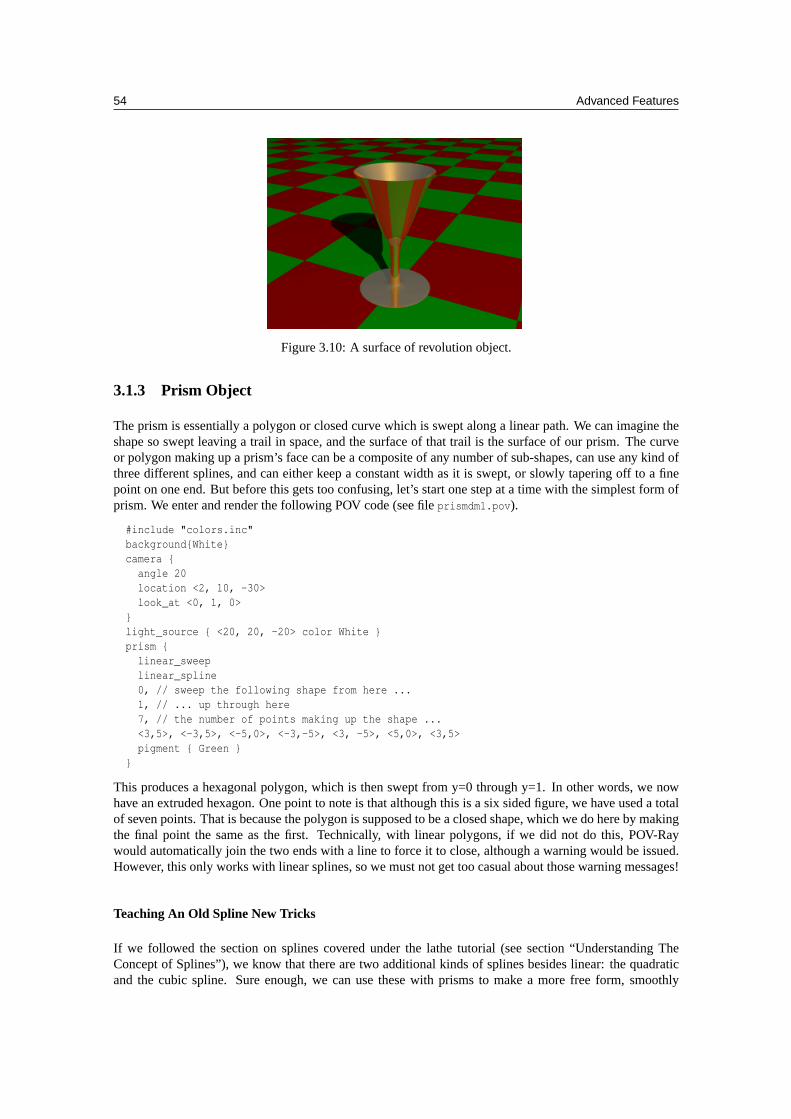
54 Advanced Features
Figure 3.10: A surface of revolution object.
3.1.3 Prism Object
The prism is essentially a polygon or closed curve which is swept along a linear path. We can imagine theshape so swept leaving a trail in space, and the surface of that trail is the surface of our prism. The curveor polygon making up a prism’s face can be a composite of any number of sub-shapes, can use any kind ofthree different splines, and can either keep a constant width as it is swept, or slowly tapering off to a finepoint on one end. But before this gets too confusing, let’s start one step at a time with the simplest form ofprism. We enter and render the following POV code (see fileprismdm1.pov).
#include "colors.inc"background{White}camera {
angle 20location <2, 10, -30>look_at <0, 1, 0>
}light_source { <20, 20, -20> color White }prism {
linear_sweeplinear_spline0, // sweep the following shape from here ...1, // ... up through here7, // the number of points making up the shape ...<3,5>, <-3,5>, <-5,0>, <-3,-5>, <3, -5>, <5,0>, <3,5>pigment { Green }
}
This produces a hexagonal polygon, which is then swept from y=0 through y=1. In other words, we nowhave an extruded hexagon. One point to note is that although this is a six sided figure, we have used a totalof seven points. That is because the polygon is supposed to be a closed shape, which we do here by makingthe final point the same as the first. Technically, with linear polygons, if we did not do this, POV-Raywould automatically join the two ends with a line to force it to close, although a warning would be issued.However, this only works with linear splines, so we must not get too casual about those warning messages!
Teaching An Old Spline New Tricks
If we followed the section on splines covered under the lathe tutorial (see section “Understanding TheConcept of Splines”), we know that there are two additional kinds of splines besides linear: the quadraticand the cubic spline. Sure enough, we can use these with prisms to make a more free form, smoothly
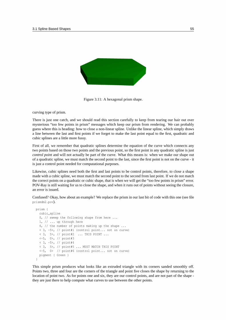
3.1 Spline Based Shapes 55
Figure 3.11: A hexagonal prism shape.
curving type of prism.
There is just one catch, and we should read this section carefully to keep from tearing our hair out overmysterious “too few points in prism” messages which keep our prism from rendering. We can probablyguess where this is heading: how to close a non-linear spline. Unlike the linear spline, which simply drawsa line between the last and first points if we forget to make the last point equal to the first, quadratic andcubic splines are a little more fussy.
First of all, we remember that quadratic splines determine the equation of the curve which connects anytwo points based on those two points and the previous point, so the first point in any quadratic spline is justcontrol pointand will not actually be part of the curve. What this means is: when we make our shape outof a quadratic spline, we must match the second point to the last, since the first point is not on the curve - itis just a control point needed for computational purposes.
Likewise, cubic splines need both the first and last points to be control points, therefore, to close a shapemade with a cubic spline, we must match the second point to the second from last point. If we do not matchthe correct points on a quadratic or cubic shape, that is when we will get the “too few points in prism” error.POV-Ray is still waiting for us to close the shape, and when it runs out of points without seeing the closure,an error is issued.
Confused? Okay, how about an example? We replace the prism in our last bit of code with this one (see fileprismdm2.pov).
prism {cubic_spline0, // sweep the following shape from here ...1, // ... up through here6, // the number of points making up the shape ...< 3, -5>, // point#1 (control point... not on curve)< 3, 5>, // point#2 ... THIS POINT ...<-5, 0>, // point#3< 3, -5>, // point#4< 3, 5>, // point#5 ... MUST MATCH THIS POINT<-5, 0> // point#6 (control point... not on curve)pigment { Green }
}
This simple prism produces what looks like an extruded triangle with its corners sanded smoothly off.Points two, three and four are the corners of the triangle and point five closes the shape by returning to thelocation of point two. As for points one and six, they are our control points, and are not part of the shape -they are just there to help compute what curves to use between the other points.
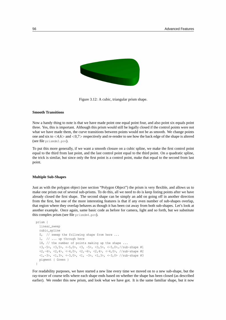
56 Advanced Features
Figure 3.12: A cubic, triangular prism shape.
Smooth Transitions
Now a handy thing to note is that we have made point one equal point four, and also point six equals pointthree. Yes, this is important. Although this prism would still be legally closed if the control points were notwhat we have made them, the curve transitions between points would not be as smooth. We change pointsone and six to<4,6> and<0,7> respectively and re-render to see how the back edge of the shape is altered(see fileprismdm3.pov).
To put this more generally, if we want a smooth closure on a cubic spline, we make the first control pointequal to the third from last point, and the last control point equal to the third point. On a quadratic spline,the trick is similar, but since only the first point is a control point, make that equal to the second from lastpoint.
Multiple Sub-Shapes
Just as with the polygon object (see section “Polygon Object”) the prism is very flexible, and allows us tomake one prism out of several sub-prisms. To do this, all we need to do is keep listing points after we havealready closed the first shape. The second shape can be simply an add on going off in another directionfrom the first, but one of the more interesting features is that if any even number of sub-shapes overlap,that region where they overlap behaves as though it has been cut away from both sub-shapes. Let’s look atanother example. Once again, same basic code as before for camera, light and so forth, but we substitutethis complex prism (see fileprismdm4.pov).
prism {linear_sweepcubic_spline0, // sweep the following shape from here ...1, // ... up through here18, // the number of points making up the shape ...<3,-5>, <3,5>, <-5,0>, <3, -5>, <3,5>, <-5,0>,//sub-shape #1<2,-4>, <2,4>, <-4,0>, <2,-4>, <2,4>, <-4,0>, //sub-shape #2<1,-3>, <1,3>, <-3,0>, <1, -3>, <1,3>, <-3,0> //sub-shape #3pigment { Green }
}
For readability purposes, we have started a new line every time we moved on to a new sub-shape, but theray-tracer of course tells where each shape ends based on whether the shape has been closed (as describedearlier). We render this new prism, and look what we have got. It is the same familiar shape, but it now
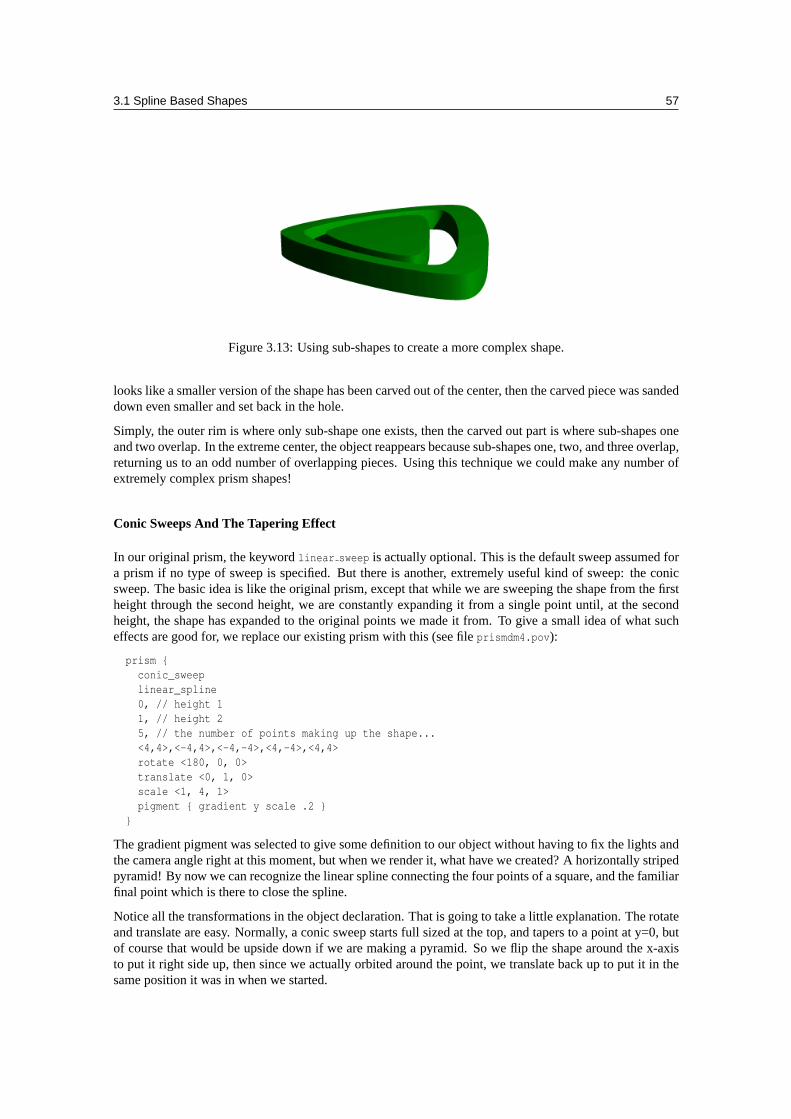
3.1 Spline Based Shapes 57
Figure 3.13: Using sub-shapes to create a more complex shape.
looks like a smaller version of the shape has been carved out of the center, then the carved piece was sandeddown even smaller and set back in the hole.
Simply, the outer rim is where only sub-shape one exists, then the carved out part is where sub-shapes oneand two overlap. In the extreme center, the object reappears because sub-shapes one, two, and three overlap,returning us to an odd number of overlapping pieces. Using this technique we could make any number ofextremely complex prism shapes!
Conic Sweeps And The Tapering Effect
In our original prism, the keywordlinear sweep is actually optional. This is the default sweep assumed fora prism if no type of sweep is specified. But there is another, extremely useful kind of sweep: the conicsweep. The basic idea is like the original prism, except that while we are sweeping the shape from the firstheight through the second height, we are constantly expanding it from a single point until, at the secondheight, the shape has expanded to the original points we made it from. To give a small idea of what sucheffects are good for, we replace our existing prism with this (see fileprismdm4.pov):
prism {conic_sweeplinear_spline0, // height 11, // height 25, // the number of points making up the shape...<4,4>,<-4,4>,<-4,-4>,<4,-4>,<4,4>rotate <180, 0, 0>translate <0, 1, 0>scale <1, 4, 1>pigment { gradient y scale .2 }
}
The gradient pigment was selected to give some definition to our object without having to fix the lights andthe camera angle right at this moment, but when we render it, what have we created? A horizontally stripedpyramid! By now we can recognize the linear spline connecting the four points of a square, and the familiarfinal point which is there to close the spline.
Notice all the transformations in the object declaration. That is going to take a little explanation. The rotateand translate are easy. Normally, a conic sweep starts full sized at the top, and tapers to a point at y=0, butof course that would be upside down if we are making a pyramid. So we flip the shape around the x-axisto put it right side up, then since we actually orbited around the point, we translate back up to put it in thesame position it was in when we started.
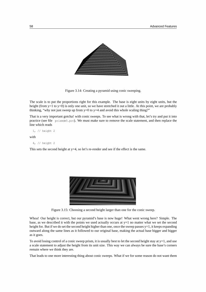
58 Advanced Features
Figure 3.14: Creating a pyramid using conic sweeping.
The scale is to put the proportions right for this example. The base is eight units by eight units, but theheight (from y=1 to y=0) is only one unit, so we have stretched it out a little. At this point, we are probablythinking, “why not just sweep up from y=0 to y=4 and avoid this whole scaling thing?”
That is a very important gotcha! with conic sweeps. To see what is wrong with that, let’s try and put it intopractice (see fileprismdm5.pov). We must make sure to remove the scale statement, and then replace theline which reads
1, // height 2
with
4, // height 2
This sets the second height at y=4, so let’s re-render and see if the effect is the same.
Figure 3.15: Choosing a second height larger than one for the conic sweep.
Whoa! Our height is correct, but our pyramid’s base is now huge! What went wrong here? Simple. Thebase, as we described it with the points we used actually occurs at y=1 no matter what we set the secondheight for. But if we do set the second height higher than one, once the sweep passes y=1, it keeps expandingoutward along the same lines as it followed to our original base, making the actual base bigger and biggeras it goes.
To avoid losing control of a conic sweep prism, it is usually best to let the second height stay at y=1, and usea scale statement to adjust the height from its unit size. This way we can always be sure the base’s cornersremain where we think they are.
That leads to one more interesting thing about conic sweeps. What if we for some reason do not want them
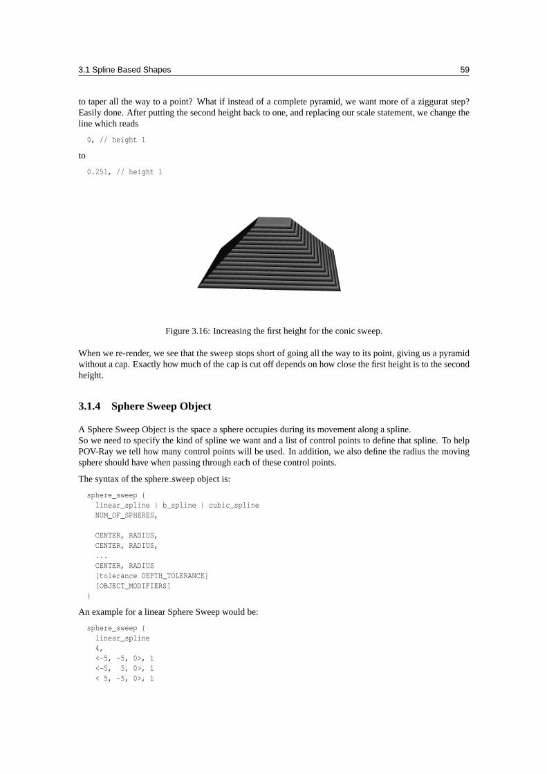
3.1 Spline Based Shapes 59
to taper all the way to a point? What if instead of a complete pyramid, we want more of a ziggurat step?Easily done. After putting the second height back to one, and replacing our scale statement, we change theline which reads
0, // height 1
to
0.251, // height 1
Figure 3.16: Increasing the first height for the conic sweep.
When we re-render, we see that the sweep stops short of going all the way to its point, giving us a pyramidwithout a cap. Exactly how much of the cap is cut off depends on how close the first height is to the secondheight.
3.1.4 Sphere Sweep Object
A Sphere Sweep Object is the space a sphere occupies during its movement along a spline.So we need to specify the kind of spline we want and a list of control points to define that spline. To helpPOV-Ray we tell how many control points will be used. In addition, we also define the radius the movingsphere should have when passing through each of these control points.
The syntax of the spheresweep object is:
sphere_sweep {linear_spline | b_spline | cubic_splineNUM_OF_SPHERES,
CENTER, RADIUS,CENTER, RADIUS,...CENTER, RADIUS[tolerance DEPTH_TOLERANCE][OBJECT_MODIFIERS]
}
An example for a linear Sphere Sweep would be:
sphere_sweep {linear_spline4,<-5, -5, 0>, 1<-5, 5, 0>, 1< 5, -5, 0>, 1
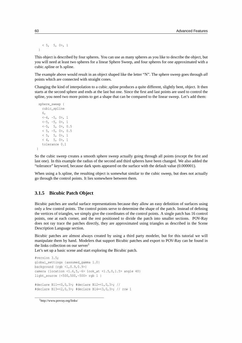
60 Advanced Features
< 5, 5, 0>, 1}
This object is described by four spheres. You can use as many spheres as you like to describe the object, butyou will need at least two spheres for a linear Sphere Sweep, and four spheres for one approximated with acubic spline or bspline.
The example above would result in an object shaped like the letter “N”. The sphere sweep goes throughallpoints which are connected with straight cones.
Changing the kind of interpolation to a cubicspline produces a quite different, slightly bent, object. It thenstarts at the second sphere and ends at the last but one. Since the first and last points are used to control thespline, you need two more points to get a shape that can be compared to the linear sweep. Let’s add them:
sphere_sweep {cubic_spline6,<-4, -5, 0>, 1<-5, -5, 0>, 1<-5, 5, 0>, 0.5< 5, -5, 0>, 0.5< 5, 5, 0>, 1< 4, 5, 0>, 1tolerance 0.1
}
So the cubic sweep creates a smooth sphere sweep actually going through all points (except the first andlast one). In this example the radius of the second and third spheres have been changed. We also added the“tolerance” keyword, because dark spots appeared on the surface with the default value (0.000001).
When using a bspline, the resulting object is somewhat similar to the cubic sweep, but does not actuallygo through the control points. It lies somewhere between them.
3.1.5 Bicubic Patch Object
Bicubic patches are useful surface representations because they allow an easy definition of surfaces usingonly a few control points. The control points serve to determine the shape of the patch. Instead of definingthe vertices of triangles, we simply give the coordinates of the control points. A single patch has 16 controlpoints, one at each corner, and the rest positioned to divide the patch into smaller sections. POV-Raydoes not ray trace the patches directly, they are approximated using triangles as described in the SceneDescription Language section.
Bicubic patches are almost always created by using a third party modeler, but for this tutorial we willmanipulate them by hand. Modelers that support Bicubic patches and export to POV-Ray can be found inthe links collection on our server1
Let’s set up a basic scene and start exploring the Bicubic patch.
#version 3.5;global_settings {assumed_gamma 1.0}background {rgb <1,0.9,0.9>}camera {location <1.6,5,-6> look_at <1.5,0,1.5> angle 40}light_source {<500,500,-500> rgb 1 }
#declare B11=<0,0,3>; #declare B12=<1,0,3>; //#declare B13=<2,0,3>; #declare B14=<3,0,3>; // row 1
1http://www.povray.org/links/
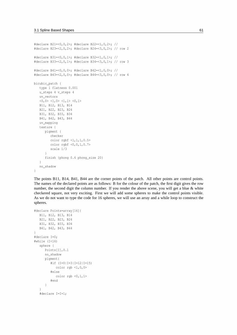
3.1 Spline Based Shapes 61
#declare B21=<0,0,2>; #declare B22=<1,0,2>; //#declare B23=<2,0,2>; #declare B24=<3,0,2>; // row 2
#declare B31=<0,0,1>; #declare B32=<1,0,1>; //#declare B33=<2,0,1>; #declare B34=<3,0,1>; // row 3
#declare B41=<0,0,0>; #declare B42=<1,0,0>; //#declare B43=<2,0,0>; #declare B44=<3,0,0>; // row 4
bicubic_patch {type 1 flatness 0.001u_steps 4 v_steps 4uv_vectors<0,0> <1,0> <1,1> <0,1>B11, B12, B13, B14B21, B22, B23, B24B31, B32, B33, B34B41, B42, B43, B44uv_mappingtexture {
pigment {checkercolor rgbf <1,1,1,0.5>color rgbf <0,0,1,0.7>scale 1/3
}finish {phong 0.6 phong_size 20}
}no_shadow
}
The points B11, B14, B41, B44 are the corner points of the patch. All other points are control points.The names of the declared points are as follows: B for the colour of the patch, the first digit gives the rownumber, the second digit the column number. If you render the above scene, you will get a blue & whitecheckered square, not very exciting. First we will add some spheres to make the control points visible.As we do not want to type the code for 16 spheres, we will use an array and a while loop to construct thespheres.
#declare Points=array[16]{B11, B12, B13, B14B21, B22, B23, B24B31, B32, B33, B34B41, B42, B43, B44
}#declare I=0;#while (I<16)
sphere {Points[I],0.1no_shadowpigment{
#if (I=0|I=3|I=12|I=15)color rgb <1,0,0>
#elsecolor rgb <0,1,1>
#end}
}#declare I=I+1;
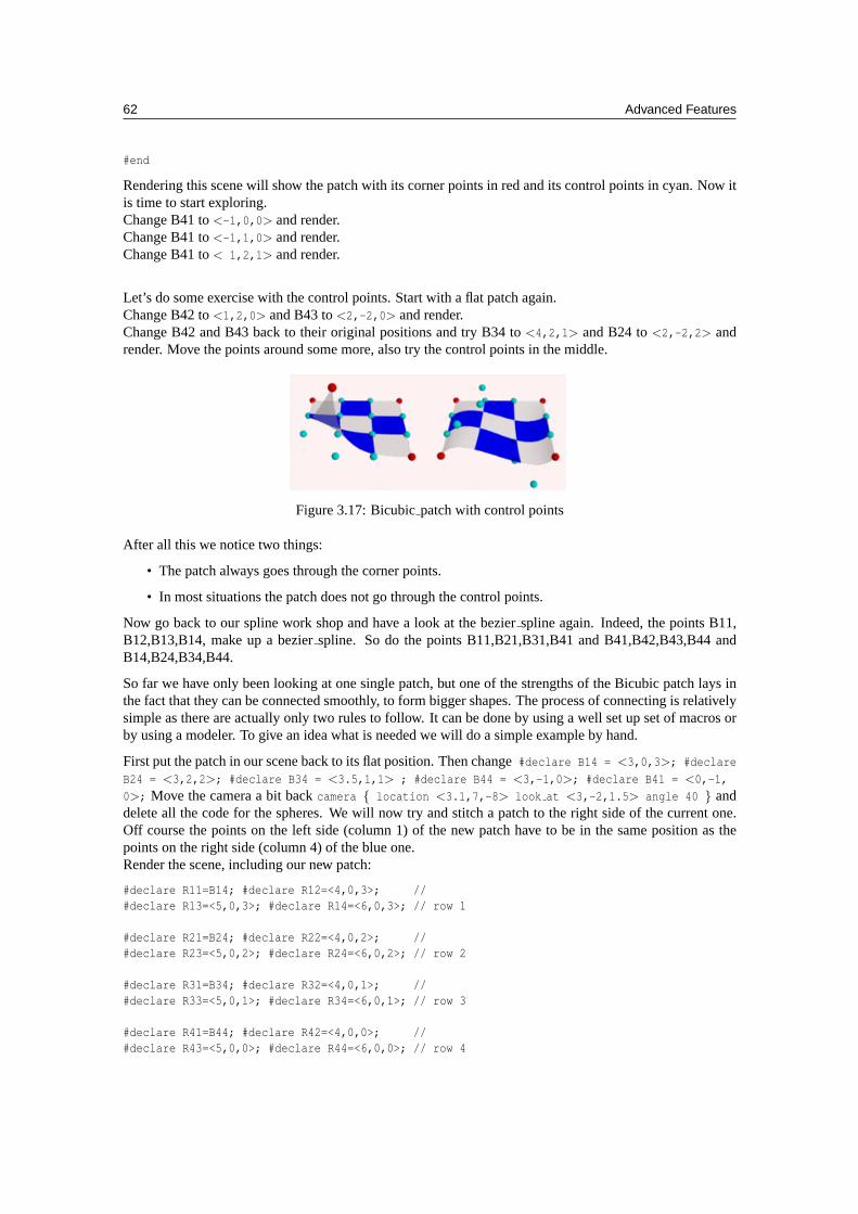
62 Advanced Features
#end
Rendering this scene will show the patch with its corner points in red and its control points in cyan. Now itis time to start exploring.Change B41 to<-1,0,0> and render.Change B41 to<-1,1,0> and render.Change B41 to< 1,2,1> and render.
Let’s do some exercise with the control points. Start with a flat patch again.Change B42 to<1,2,0> and B43 to<2,-2,0> and render.Change B42 and B43 back to their original positions and try B34 to<4,2,1> and B24 to<2,-2,2> andrender. Move the points around some more, also try the control points in the middle.
Figure 3.17: Bicubicpatch with control points
After all this we notice two things:
• The patch always goes through the corner points.
• In most situations the patch does not go through the control points.
Now go back to our spline work shop and have a look at the bezierspline again. Indeed, the points B11,B12,B13,B14, make up a bezierspline. So do the points B11,B21,B31,B41 and B41,B42,B43,B44 andB14,B24,B34,B44.
So far we have only been looking at one single patch, but one of the strengths of the Bicubic patch lays inthe fact that they can be connected smoothly, to form bigger shapes. The process of connecting is relativelysimple as there are actually only two rules to follow. It can be done by using a well set up set of macros orby using a modeler. To give an idea what is needed we will do a simple example by hand.
First put the patch in our scene back to its flat position. Then change#declare B14 = <3,0,3>; #declare
B24 = <3,2,2>; #declare B34 = <3.5,1,1> ; #declare B44 = <3,-1,0>; #declare B41 = <0,-1,
0>; Move the camera a bit backcamera { location <3.1,7,-8> look at <3,-2,1.5> angle 40 } anddelete all the code for the spheres. We will now try and stitch a patch to the right side of the current one.Off course the points on the left side (column 1) of the new patch have to be in the same position as thepoints on the right side (column 4) of the blue one.Render the scene, including our new patch:
#declare R11=B14; #declare R12=<4,0,3>; //#declare R13=<5,0,3>; #declare R14=<6,0,3>; // row 1
#declare R21=B24; #declare R22=<4,0,2>; //#declare R23=<5,0,2>; #declare R24=<6,0,2>; // row 2
#declare R31=B34; #declare R32=<4,0,1>; //#declare R33=<5,0,1>; #declare R34=<6,0,1>; // row 3
#declare R41=B44; #declare R42=<4,0,0>; //#declare R43=<5,0,0>; #declare R44=<6,0,0>; // row 4
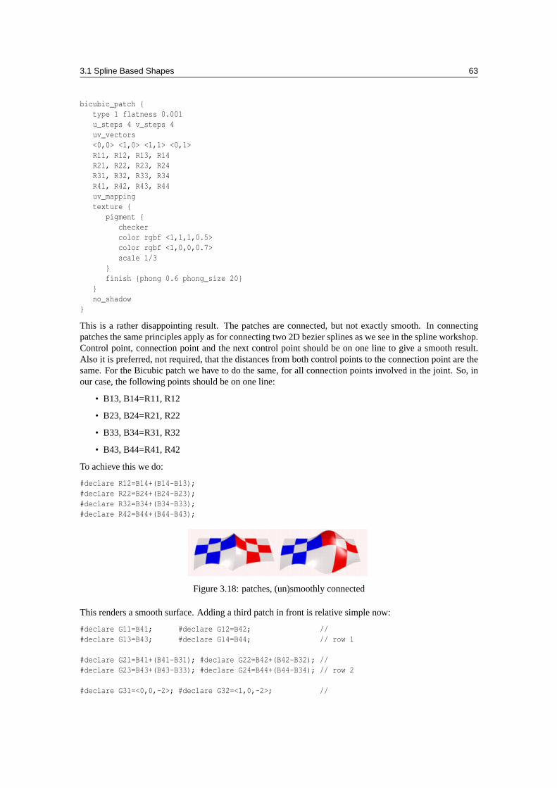
3.1 Spline Based Shapes 63
bicubic_patch {type 1 flatness 0.001u_steps 4 v_steps 4uv_vectors<0,0> <1,0> <1,1> <0,1>R11, R12, R13, R14R21, R22, R23, R24R31, R32, R33, R34R41, R42, R43, R44uv_mappingtexture {
pigment {checkercolor rgbf <1,1,1,0.5>color rgbf <1,0,0,0.7>scale 1/3
}finish {phong 0.6 phong_size 20}
}no_shadow
}
This is a rather disappointing result. The patches are connected, but not exactly smooth. In connectingpatches the same principles apply as for connecting two 2D bezier splines as we see in the spline workshop.Control point, connection point and the next control point should be on one line to give a smooth result.Also it is preferred, not required, that the distances from both control points to the connection point are thesame. For the Bicubic patch we have to do the same, for all connection points involved in the joint. So, inour case, the following points should be on one line:
• B13, B14=R11, R12
• B23, B24=R21, R22
• B33, B34=R31, R32
• B43, B44=R41, R42
To achieve this we do:
#declare R12=B14+(B14-B13);#declare R22=B24+(B24-B23);#declare R32=B34+(B34-B33);#declare R42=B44+(B44-B43);
Figure 3.18: patches, (un)smoothly connected
This renders a smooth surface. Adding a third patch in front is relative simple now:
#declare G11=B41; #declare G12=B42; //#declare G13=B43; #declare G14=B44; // row 1
#declare G21=B41+(B41-B31); #declare G22=B42+(B42-B32); //#declare G23=B43+(B43-B33); #declare G24=B44+(B44-B34); // row 2
#declare G31=<0,0,-2>; #declare G32=<1,0,-2>; //
64 Advanced Features
#declare G33=<2,0,-2>; #declare G34=<3,2,-2>; // row 3
#declare G41=<0,0,-3>; #declare G42=<1,0,-3>; //#declare G43=<2,0,-3>; #declare G44=<3,0,-3> // row 4
bicubic_patch {type 1 flatness 0.001u_steps 4 v_steps 4uv_vectors<0,0> <1,0> <1,1> <0,1>G11, G12, G13, G14G21, G22, G23, G24G31, G32, G33, G34G41, G42, G43, G44uv_mappingtexture {
pigment {checkercolor rgbf <1,1,1,0.5>color rgbf <0,1,0,0.7>scale 1/3
}finish {phong 0.6 phong_size 20}
}no_shadow
}
Finally, let’s put a few spheres back in the scene and add some cylinders to visualize what is going on. Seewhat happens if you move for example B44, B43, B33 or B34.
#declare Points=array[8]{B33,B34,R32,B43,B44,R42,G23,G24}#declare I=0;#while (I<8)
sphere {Points[I],0.1no_shadowpigment{
#if (I=4)color rgb <1,0,0>
#elsecolor rgb <0,1,1>
#end}
}#declare I=I+1;
#endunion {
cylinder {B33,B34,0.04} cylinder {B34,R32,0.04}cylinder {B43,B44,0.04} cylinder {B44,R42,0.04}cylinder {G23,G24,0.04}cylinder {B33,B43,0.04} cylinder {B43,G23,0.04}cylinder {B34,B44,0.04} cylinder {B44,G24,0.04}cylinder {R32,R42,0.04}no_shadowpigment {color rgb <1,1,0>}
}
The hard part in using the Bicubic patch is not in connecting several patches. The difficulty is keepingcontrol over the shape you want to build. As patches are added, in order to keep the result smooth, control
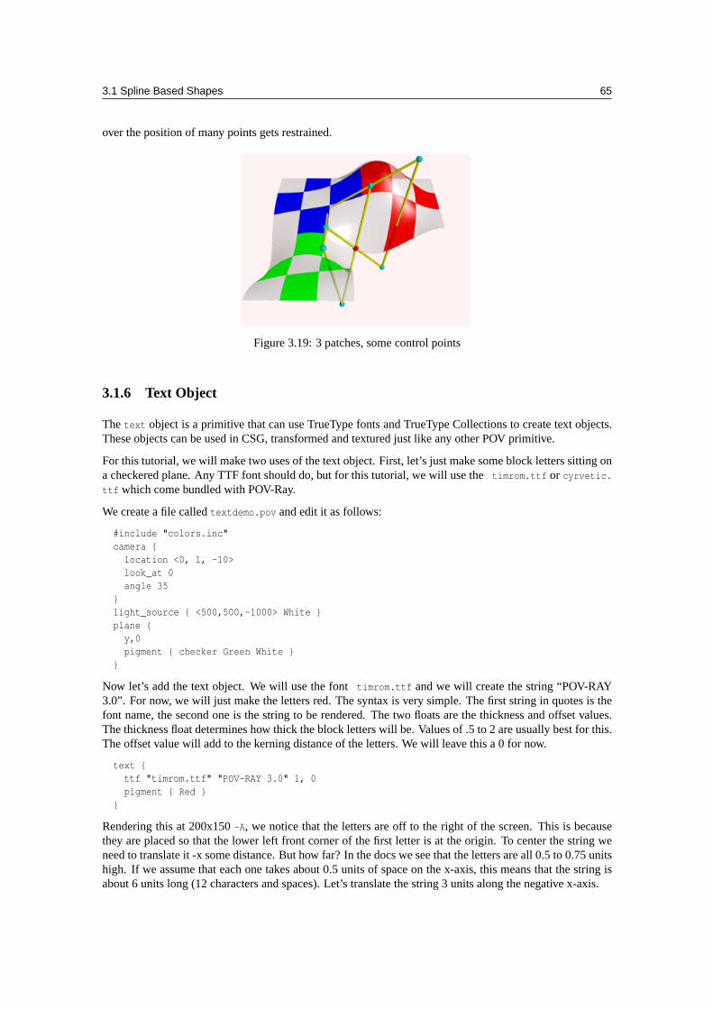
3.1 Spline Based Shapes 65
over the position of many points gets restrained.
Figure 3.19: 3 patches, some control points
3.1.6 Text Object
Thetext object is a primitive that can use TrueType fonts and TrueType Collections to create text objects.These objects can be used in CSG, transformed and textured just like any other POV primitive.
For this tutorial, we will make two uses of the text object. First, let’s just make some block letters sitting ona checkered plane. Any TTF font should do, but for this tutorial, we will use thetimrom.ttf or cyrvetic.ttf which come bundled with POV-Ray.
We create a file calledtextdemo.pov and edit it as follows:
#include "colors.inc"camera {
location <0, 1, -10>look_at 0angle 35
}light_source { <500,500,-1000> White }plane {
y,0pigment { checker Green White }
}
Now let’s add the text object. We will use the fonttimrom.ttf and we will create the string “POV-RAY3.0”. For now, we will just make the letters red. The syntax is very simple. The first string in quotes is thefont name, the second one is the string to be rendered. The two floats are the thickness and offset values.The thickness float determines how thick the block letters will be. Values of .5 to 2 are usually best for this.The offset value will add to the kerning distance of the letters. We will leave this a 0 for now.
text {ttf "timrom.ttf" "POV-RAY 3.0" 1, 0pigment { Red }
}
Rendering this at 200x150-A, we notice that the letters are off to the right of the screen. This is becausethey are placed so that the lower left front corner of the first letter is at the origin. To center the string weneed to translate it -x some distance. But how far? In the docs we see that the letters are all 0.5 to 0.75 unitshigh. If we assume that each one takes about 0.5 units of space on the x-axis, this means that the string isabout 6 units long (12 characters and spaces). Let’s translate the string 3 units along the negative x-axis.
66 Advanced Features
text {ttf "timrom.ttf" "POV-RAY 3.0" 1, 0pigment { Red }translate -3*x
}
That is better. Now let’s play around with some of the parameters of the text object. First, let’s raise thethickness float to something outlandish... say 25!
text {ttf "timrom.ttf" "POV-RAY 3.0" 25, 0pigment { Red }translate -2.25*x
}
Actually, that is kind of cool. Now let’s return the thickness value to 1 and try a different offset value.Change the offset float from 0 to 0.1 and render it again.
Wait a minute?! The letters go wandering off up at an angle! That is not what the docs describe! It almostlooks as if the offset value applies in both the x- and y-axis instead of just the x axis like we intended. Couldit be that a vector is called for here instead of a float? Let’s try it. We replace0.1 with 0.1*x and render itagain.
That works! The letters are still in a straight line along the x-axis, just a little further apart. Let’s verify thisand try to offset just in the y-axis. We replace0.1*x with 0.1*y. Again, this works as expected with theletters going up to the right at an angle with no additional distance added along the x-axis. Now let’s trythe z-axis. We replace0.1*y with 0.1*z. Rendering this yields a disappointment. No offset occurs! Theoffset value can only be applied in the x- and y-directions.
Let’s finish our scene by giving a fancier texture to the block letters, using that cool large thickness value,and adding a slight y-offset. For fun, we will throw in a sky sphere, dandy up our plane a bit, and use a littlemore interesting camera viewpoint (we render the following scene at 640x480+A0.2):
#include "colors.inc"camera {
location <-5,.15,-2>look_at <.3,.2,1>angle 35
}light_source { <500,500,-1000> White }plane {
y,0texture {
pigment { SeaGreen }finish { reflection .35 specular 1 }normal { ripples .35 turbulence .5 scale .25 }
}}text {
ttf "timrom.ttf" "POV-RAY 3.0" 25, 0.1*ypigment { BrightGold }finish { reflection .25 specular 1 }translate -3*x
}#include "skies.inc"sky_sphere { S_Cloud5 }
Let’s try using text in a CSG object. We will attempt to create an inlay in a stone block using a text object.We create a new file calledtextcsg.pov and edit it as follows:
3.2 Polygon Based Shapes 67
#include "colors.inc"#include "stones.inc"background { color rgb 1 }camera {
location <-3, 5, -15>look_at 0angle 25
}light_source { <500,500,-1000> White }
Now let’s create the block. We want it to be about eight units across because our text string “POV-RAY3.0” is about six units long. We also want it about four units high and about one unit deep. But we need toavoid a potential coincident surface with the text object so we will make the first z-coordinate 0.1 insteadof 0. Finally, we will give this block a nice stone texture.
box {<-3.5, -1, 0.1>, <3.5, 1, 1>texture { T_Stone10 }
}
Next, we want to make the text object. We can use the same object we used in the first tutorial except wewill use slightly different thickness and offset values.
text {ttf "timrom.ttf" "POV-RAY 3.0" 0.15, 0pigment { BrightGold }finish { reflection .25 specular 1 }translate -3*x
}
We remember that the text object is placed by default so that its front surface lies directly on the x-y-plane.If the front of the box begins at z=0.1 and thickness is set at 0.15, the depth of the inlay will be 0.05 units.We place a difference block around the two objects.
difference {box {
<-3.5, -1, 0.1>, <3.5, 1, 1>texture { T_Stone10 }
}text {
ttf "timrom.ttf" "POV-RAY 3.0" 0.15, 0pigment { BrightGold }finish { reflection .25 specular 1 }translate -3*x
}}
We render this at 200x150-A. We can see the inlay clearly and that it is indeed a bright gold color. Were-render at 640x480+A0.2 to see the results more clearly, but be forewarned... this trace will take a littletime.
3.2 Polygon Based Shapes
3.2.1 Mesh Object
You know you have been raytracing too long when ...... You think that the evolution theory was based on the triangular origin of the wheel.
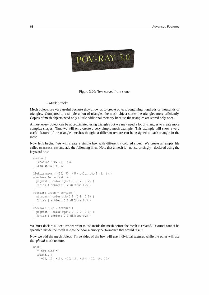
68 Advanced Features
Figure 3.20: Text carved from stone.
– Mark Kadela
Mesh objects are very useful because they allow us to create objects containing hundreds or thousands oftriangles. Compared to a simple union of triangles the mesh object stores the triangles more efficiently.Copies of mesh objects need only a little additional memory because the triangles are stored only once.
Almost every object can be approximated using triangles but we may need a lot of triangles to create morecomplex shapes. Thus we will only create a very simple mesh example. This example will show a veryuseful feature of the triangles meshes though: a different texture can be assigned to each triangle in themesh.
Now let’s begin. We will create a simple box with differently colored sides. We create an empty filecalledmeshdemo.pov and add the following lines. Note that a mesh is - not surprisingly - declared using thekeywordmesh.
camera {location <20, 20, -50>look_at <0, 5, 0>
}light_source { <50, 50, -50> color rgb<1, 1, 1> }#declare Red = texture {
pigment { color rgb<0.8, 0.2, 0.2> }finish { ambient 0.2 diffuse 0.5 }
}#declare Green = texture {
pigment { color rgb<0.2, 0.8, 0.2> }finish { ambient 0.2 diffuse 0.5 }
}#declare Blue = texture {
pigment { color rgb<0.2, 0.2, 0.8> }finish { ambient 0.2 diffuse 0.5 }
}
We must declare all textures we want to use inside the mesh before the mesh is created. Textures cannot bespecified inside the mesh due to the poor memory performance that would result.
Now we add the mesh object. Three sides of the box will use individual textures while the other will usethe globalmesh texture.
mesh {/* top side */triangle {
<-10, 10, -10>, <10, 10, -10>, <10, 10, 10>
3.2 Polygon Based Shapes 69
texture { Red }}triangle {
<-10, 10, -10>, <-10, 10, 10>, <10, 10, 10>texture { Red }
}/* bottom side */triangle { <-10, -10, -10>, <10, -10, -10>, <10, -10, 10> }triangle { <-10, -10, -10>, <-10, -10, 10>, <10, -10, 10> }/* left side */triangle { <-10, -10, -10>, <-10, -10, 10>, <-10, 10, 10> }triangle { <-10, -10, -10>, <-10, 10, -10>, <-10, 10, 10> }/* right side */triangle {
<10, -10, -10>, <10, -10, 10>, <10, 10, 10>texture { Green }
}triangle {
<10, -10, -10>, <10, 10, -10>, <10, 10, 10>texture { Green }
}/* front side */triangle {
<-10, -10, -10>, <10, -10, -10>, <-10, 10, -10>texture { Blue }
}triangle {
<-10, 10, -10>, <10, 10, -10>, <10, -10, -10>texture { Blue }
}/* back side */triangle { <-10, -10, 10>, <10, -10, 10>, <-10, 10, 10> }triangle { <-10, 10, 10>, <10, 10, 10>, <10, -10, 10> }texture {
pigment { color rgb<0.9, 0.9, 0.9> }finish { ambient 0.2 diffuse 0.7 }
}}
Tracing the scene at 320x240 we will see that the top, right and front side of the box have different textures.Though this is not a very impressive example it shows what we can do with mesh objects. More complexexamples, also using smooth triangles, can be found under the scene directory aschesmsh.pov.
3.2.2 Mesh2 Object
The mesh2 is a representation of a mesh, that is much more like POV-Ray’s internal mesh representationthan the standardmesh. As a result, it parses faster and it file size is smaller.
Due to its nature,mesh2 is not really suitable for building meshes by hand, it is intended for use by modelersand file format converters. An other option is building the meshes by macros. Yet, to understand the format,we will do a small example by hand and go through all options.
We will turn the mesh sketched above into amesh2 object. The mesh is made of 8 triangles, each with 3vertices, many of these vertices are shared among the triangles. This can later be used to optimize the mesh.First we will set it up straight forward.
In mesh2 all the vertices are listed in a list namedvertex vectors{}. A second list,face indices{}, tells us
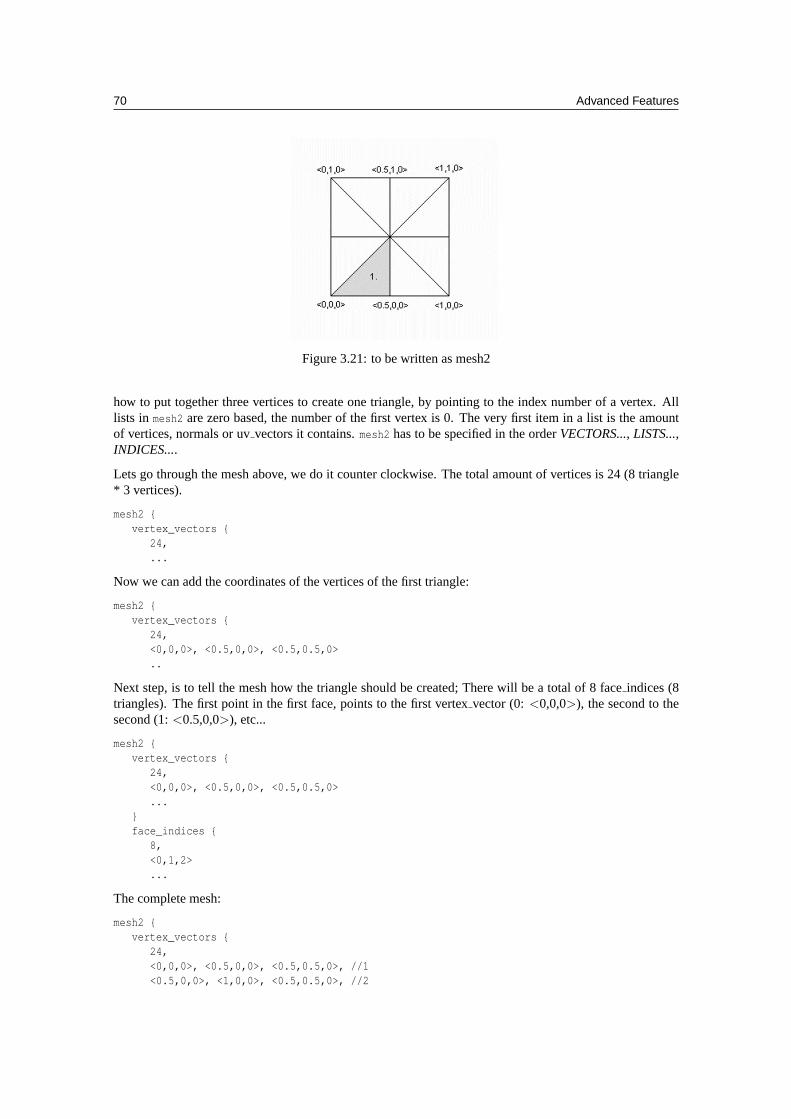
70 Advanced Features
Figure 3.21: to be written as mesh2
how to put together three vertices to create one triangle, by pointing to the index number of a vertex. Alllists in mesh2 are zero based, the number of the first vertex is 0. The very first item in a list is the amountof vertices, normals or uvvectors it contains.mesh2 has to be specified in the orderVECTORS..., LISTS...,INDICES....
Lets go through the mesh above, we do it counter clockwise. The total amount of vertices is 24 (8 triangle* 3 vertices).
mesh2 {vertex_vectors {
24,...
Now we can add the coordinates of the vertices of the first triangle:
mesh2 {vertex_vectors {
24,<0,0,0>, <0.5,0,0>, <0.5,0.5,0>..
Next step, is to tell the mesh how the triangle should be created; There will be a total of 8 faceindices (8triangles). The first point in the first face, points to the first vertexvector (0:<0,0,0>), the second to thesecond (1:<0.5,0,0>), etc...
mesh2 {vertex_vectors {
24,<0,0,0>, <0.5,0,0>, <0.5,0.5,0>...
}face_indices {
8,<0,1,2>...
The complete mesh:
mesh2 {vertex_vectors {
24,<0,0,0>, <0.5,0,0>, <0.5,0.5,0>, //1<0.5,0,0>, <1,0,0>, <0.5,0.5,0>, //2
3.2 Polygon Based Shapes 71
<1,0,0>, <1,0.5,0>, <0.5,0.5,0>, //3<1,0.5,0>, <1,1,0>, <0.5,0.5,0>, //4<1,1,0>, <0.5,1,0>, <0.5,0.5,0>, //5<0.5,1,0>, <0,1,0>, <0.5,0.5,0>, //6<0,1,0>, <0,0.5,0>, <0.5,0.5,0>, //7<0,0.5,0>, <0,0,0>, <0.5,0.5,0> //8
}face_indices {
8,<0,1,2>, <3,4,5>, //1 2<6,7,8>, <9,10,11>, //3 4<12,13,14>, <15,16,17>, //5 6<18,19,20>, <21,22,23> //7 8
}pigment {rgb 1}
}
As mentioned earlier, many vertices are shared by triangles. We can optimize the mesh by removing allduplicate vertices but one. In the example this reduces the amount from 24 to 9.
mesh2 {vertex_vectors {
9,<0,0,0>, <0.5,0,0>, <0.5,0.5,0>,/*as 1*/ <1,0,0>, /*as 2*//*as 3*/ <1,0.5,0>, /*as 2*//*as 4*/ <1,1,0>, /*as 2*//*as 5*/ <0.5,1,0>, /*as 2*//*as 6*/ <0,1,0>, /*as 2*//*as 7*/ <0,0.5,0>, /*as 2*//*as 8*/ /*as 0*/ /*as 2*/
}......
Next step is to rebuild the list of faceindices, as they now point to indices in thevertex vector{} list thatdo not exist anymore.
...
...face_indices {
8,<0,1,2>, <1,3,2>,<3,4,2>, <4,5,2>,<5,6,2>, <6,7,2>,<7,8,2>, <8,0,2>
}pigment {rgb 1}
}
Smooth triangles and mesh2
In case we want a smooth mesh, the same steps we did also apply to the normals in a mesh. For eachvertex there is one normal vector listed innormal vectors{}, duplicates can be removed. If the number ofnormals equals the number of vertices then thenormal indices{} list is optional and the indexes from theface indices{} list are used instead.
mesh2 {
72 Advanced Features
vertex_vectors {9,<0,0,0>, <0.5,0,0>, <0.5,0.5,0>,<1,0,0>, <1,0.5,0>, <1,1,0>,<0.5,1,0>, <0,1,0>, <0,0.5,0>
}normal_vectors {
9,<-1,-1,0>,<0,-1,0>, <0,0,1>,/*as 1*/ <1,-1,0>, /*as 2*//*as 3*/ <1,0,0>, /*as 2*//*as 4*/ <1,1,0>, /*as 2*//*as 5*/ <0,1,0>, /*as 2*//*as 6*/ <-1,1,0>, /*as 2*//*as 7*/ <-1,0,0>, /*as 2*//*as 8*/ /*as 0*/ /*as 2*/
}face_indices {
8,<0,1,2>, <1,3,2>,<3,4,2>, <4,5,2>,<5,6,2>, <6,7,2>,<7,8,2>, <8,0,2>
}pigment {rgb 1}
}
When a mesh has a mix of smooth and flat triangles a list ofnormal indices{} has to be added, where eachentry points to what vertices a normal should be applied. In the example below only the first four normalsare actually used.
mesh2 {vertex_vectors {
9,<0,0,0>, <0.5,0,0>, <0.5,0.5,0>,<1,0,0>, <1,0.5,0>, <1,1,0>,<0.5,1,0>, <0,1,0>, <0,0.5,0>
}normal_vectors {
9,<-1,-1,0>, <0,-1,0>, <0,0,1>,<1,-1,0>, <1,0,0>, <1,1,0>,<0,1,0>, <-1,1,0>, <-1,0,0>
}face_indices {
8,<0,1,2>, <1,3,2>,<3,4,2>, <4,5,2>,<5,6,2>, <6,7,2>,<7,8,2>, <8,0,2>
}normal_indices {
4,<0,1,2>, <1,3,2>,<3,4,2>, <4,5,2>
}pigment {rgb 1}
}
3.2 Polygon Based Shapes 73
UV mapping and mesh2
uv mapping is a method of ’sticking’ 2D textures on an object in such a way that it follows the form of theobject. For uvmapping on triangles imagine it as follows; First you cut out a triangular section of a textureform the xy-plane. Then stretch, shrink and deform the piece of texture to fit to the triangle and stick it on.
Now, in mesh2 we first build a list of 2D-vectors that are the coordinates of the triangular sections in thexy-plane. This is theuv vectors{} list. In the example we map the texture from the rectangular area<-0.5,-0.5>, <0.5,0.5> to the triangles in the mesh. Again we can omit all duplicate coordinates
mesh2 {vertex_vectors {
9,<0,0,0>, <0.5,0,0>, <0.5,0.5,0>,<1,0,0>, <1,0.5,0>, <1,1,0>,<0.5,1,0>, <0,1,0>, <0,0.5,0>
}uv_vectors {
9<-0.5,-0.5>,<0,-0.5>, <0,0>,/*as 1*/ <0.5,-0.5>,/*as 2*//*as 3*/ <0.5,0>, /*as 2*//*as 4*/ <0.5,0.5>, /*as 2*//*as 5*/ <0,0.5>, /*as 2*//*as 6*/ <-0.5,0.5>,/*as 2*//*as 7*/ <-0.5,0>, /*as 2*//*as 8*/ /*as 0*/ /*as 2*/
}face_indices {
8,<0,1,2>, <1,3,2>,<3,4,2>, <4,5,2>,<5,6,2>, <6,7,2>,<7,8,2>, <8,0,2>
}uv_mappingpigment {wood scale 0.2}
}
Just as with thenormal vectors, if the number ofuv vectors equals the number of vertices then theuv -
indices{} list is optional and the indices from theface indices{} list are used instead.
In contrary to thenormal indices list, if the uv indices list is used, the amount of indices should be equalto the amount offace indices. In the example below only ’one texture section’ is specified and used on alltriangles, using theuv indices.
mesh2 {vertex_vectors {
9,<0,0,0>, <0.5,0,0>, <0.5,0.5,0>,<1,0,0>, <1,0.5,0>, <1,1,0>,<0.5,1,0>, <0,1,0>, <0,0.5,0>
}uv_vectors {
3<0,0>, <0.5,0>, <0.5,0.5>
}face_indices {
8,
74 Advanced Features
<0,1,2>, <1,3,2>,<3,4,2>, <4,5,2>,<5,6,2>, <6,7,2>,<7,8,2>, <8,0,2>
}uv_indices {
8,<0,1,2>, <0,1,2>,<0,1,2>, <0,1,2>,<0,1,2>, <0,1,2>,<0,1,2>, <0,1,2>
}uv_mappingpigment {gradient x scale 0.2}
}
A separate texture per triangle
By using thetexture list it is possible to specify a texture per triangle or even per vertex in the mesh.In the latter case the three textures per triangle will be interpolated. To let POV-Ray know what texture toapply to a triangle, the index of a texture is added to theface indices list, after the face index it belongs to.
mesh2 {vertex_vectors {
9,<0,0,0>, <0.5,0,0>, <0.5,0.5,0>,<1,0,0>, <1,0.5,0>, <1,1,0><0.5,1,0>, <0,1,0>, <0,0.5,0>
}texture_list {
2,texture{pigment{rgb<0,0,1>}}texture{pigment{rgb<1,0,0>}}
}face_indices {
8,<0,1,2>,0, <1,3,2>,1,<3,4,2>,0, <4,5,2>,1,<5,6,2>,0, <6,7,2>,1,<7,8,2>,0, <8,0,2>,1
}}
To specify a texture per vertex, threetexture list indices are added after theface indices
mesh2 {vertex_vectors {
9,<0,0,0>, <0.5,0,0>, <0.5,0.5,0>,<1,0,0>, <1,0.5,0>, <1,1,0><0.5,1,0>, <0,1,0>, <0,0.5,0>
}texture_list {
3,texture{pigment{rgb <0,0,1>}}texture{pigment{rgb 1}}texture{pigment{rgb <1,0,0>}}
}
3.2 Polygon Based Shapes 75
face_indices {8,<0,1,2>,0,1,2, <1,3,2>,1,0,2,<3,4,2>,0,1,2, <4,5,2>,1,0,2,<5,6,2>,0,1,2, <6,7,2>,1,0,2,<7,8,2>,0,1,2, <8,0,2>,1,0,2
}}
Assigning a texture based on thetexture list and texture interpolation is done on a per triangle base. Soit is possible to mix triangles with just one texture and triangles with three textures in a mesh. It is evenpossible to mix in triangles without any texture indices, these will get their texture from a generaltexture
statement in themesh2. uv mapping is supported for texturing using atexture list.
3.2.3 Polygon Object
The polygon object can be used to create any planar, n-sided shapes like squares, rectangles, pentagons,hexagons, octagons, etc.
A polygon is defined by a number of points that describe its shape. Since polygons have to be closed thefirst point has to be repeated at the end of the point sequence.
In the following example we will create the word “POV” using just one polygon statement.
We start with thinking about the points we need to describe the desired shape. We want the letters to lie inthe x-y-plane with the letter O being at the center. The letters extend from y=0 to y=1. Thus we get thefollowing points for each letter (the z coordinate is automatically set to zero).
Letter P (outer polygon):
<-0.8, 0.0>, <-0.8, 1.0>,<-0.3, 1.0>, <-0.3, 0.5>,<-0.7, 0.5>, <-0.7, 0.0>
Letter P (inner polygon):
<-0.7, 0.6>, <-0.7, 0.9>,<-0.4, 0.9>, <-0.4, 0.6>
Letter O (outer polygon):
<-0.25, 0.0>, <-0.25, 1.0>,< 0.25, 1.0>, < 0.25, 0.0>
Letter O (inner polygon):
<-0.15, 0.1>, <-0.15, 0.9>,< 0.15, 0.9>, < 0.15, 0.1>
Letter V:
<0.45, 0.0>, <0.30, 1.0>,<0.40, 1.0>, <0.55, 0.1>,<0.70, 1.0>, <0.80, 1.0>,<0.65, 0.0>
Both letters P and O have a hole while the letter V consists of only one polygon. We will start with the letterV because it is easier to define than the other two letters.
We create a new file calledpolygdem.pov and add the following text.
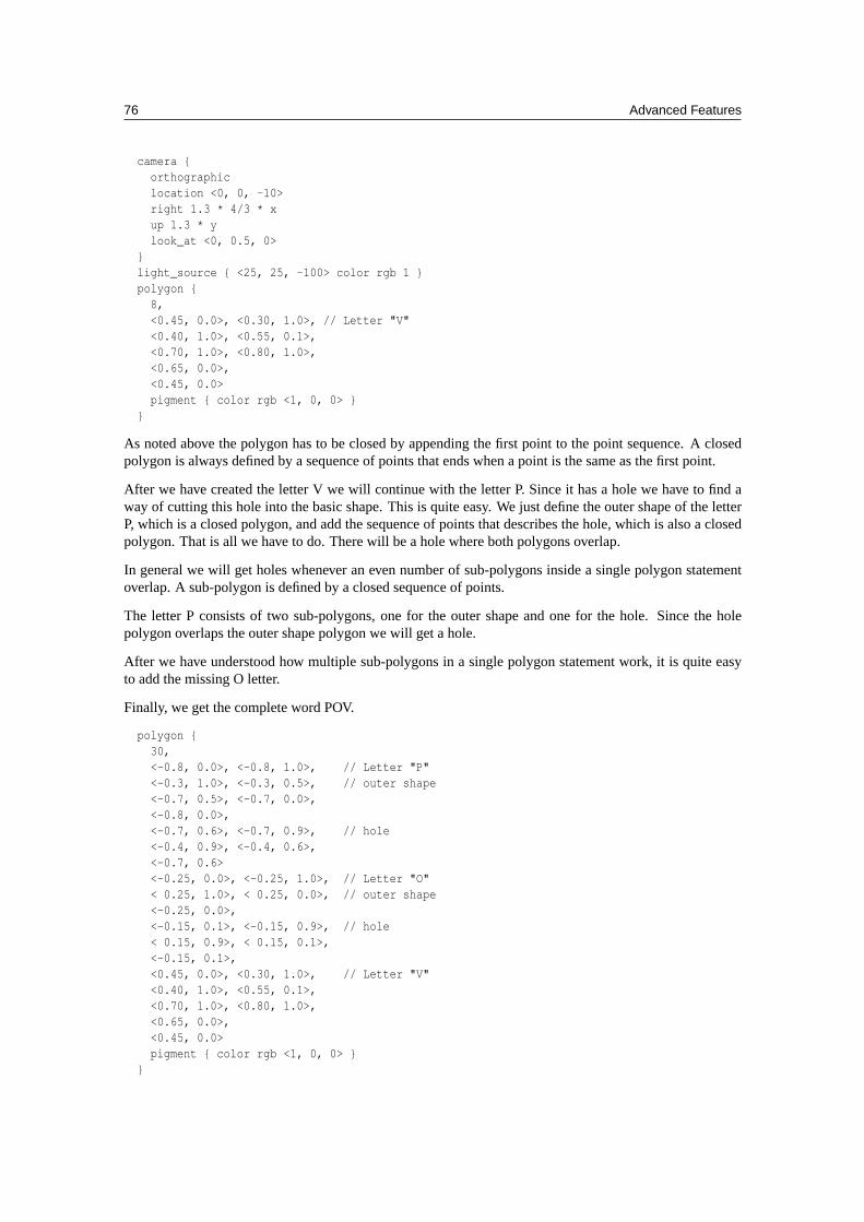
76 Advanced Features
camera {orthographiclocation <0, 0, -10>right 1.3 * 4/3 * xup 1.3 * ylook_at <0, 0.5, 0>
}light_source { <25, 25, -100> color rgb 1 }polygon {
8,<0.45, 0.0>, <0.30, 1.0>, // Letter "V"<0.40, 1.0>, <0.55, 0.1>,<0.70, 1.0>, <0.80, 1.0>,<0.65, 0.0>,<0.45, 0.0>pigment { color rgb <1, 0, 0> }
}
As noted above the polygon has to be closed by appending the first point to the point sequence. A closedpolygon is always defined by a sequence of points that ends when a point is the same as the first point.
After we have created the letter V we will continue with the letter P. Since it has a hole we have to find away of cutting this hole into the basic shape. This is quite easy. We just define the outer shape of the letterP, which is a closed polygon, and add the sequence of points that describes the hole, which is also a closedpolygon. That is all we have to do. There will be a hole where both polygons overlap.
In general we will get holes whenever an even number of sub-polygons inside a single polygon statementoverlap. A sub-polygon is defined by a closed sequence of points.
The letter P consists of two sub-polygons, one for the outer shape and one for the hole. Since the holepolygon overlaps the outer shape polygon we will get a hole.
After we have understood how multiple sub-polygons in a single polygon statement work, it is quite easyto add the missing O letter.
Finally, we get the complete word POV.
polygon {30,<-0.8, 0.0>, <-0.8, 1.0>, // Letter "P"<-0.3, 1.0>, <-0.3, 0.5>, // outer shape<-0.7, 0.5>, <-0.7, 0.0>,<-0.8, 0.0>,<-0.7, 0.6>, <-0.7, 0.9>, // hole<-0.4, 0.9>, <-0.4, 0.6>,<-0.7, 0.6><-0.25, 0.0>, <-0.25, 1.0>, // Letter "O"< 0.25, 1.0>, < 0.25, 0.0>, // outer shape<-0.25, 0.0>,<-0.15, 0.1>, <-0.15, 0.9>, // hole< 0.15, 0.9>, < 0.15, 0.1>,<-0.15, 0.1>,<0.45, 0.0>, <0.30, 1.0>, // Letter "V"<0.40, 1.0>, <0.55, 0.1>,<0.70, 1.0>, <0.80, 1.0>,<0.65, 0.0>,<0.45, 0.0>pigment { color rgb <1, 0, 0> }
}
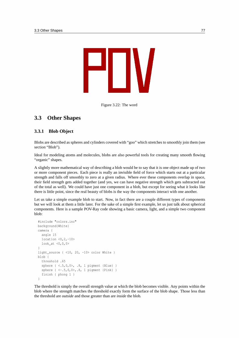
3.3 Other Shapes 77
Figure 3.22: The word
3.3 Other Shapes
3.3.1 Blob Object
Blobs are described as spheres and cylinders covered with “goo” which stretches to smoothly join them (seesection “Blob”).
Ideal for modeling atoms and molecules, blobs are also powerful tools for creating many smooth flowing“organic” shapes.
A slightly more mathematical way of describing a blob would be to say that it is one object made up of twoor more component pieces. Each piece is really an invisible field of force which starts out at a particularstrength and falls off smoothly to zero at a given radius. Where ever these components overlap in space,their field strength gets added together (and yes, we can have negative strength which gets subtracted outof the total as well). We could have just one component in a blob, but except for seeing what it looks likethere is little point, since the real beauty of blobs is the way the components interact with one another.
Let us take a simple example blob to start. Now, in fact there are a couple different types of componentsbut we will look at them a little later. For the sake of a simple first example, let us just talk about sphericalcomponents. Here is a sample POV-Ray code showing a basic camera, light, and a simple two componentblob:
#include "colors.inc"background{White}camera {
angle 15location <0,2,-10>look_at <0,0,0>
}light_source { <10, 20, -10> color White }blob {
threshold .65sphere { <.5,0,0>, .8, 1 pigment {Blue} }sphere { <-.5,0,0>,.8, 1 pigment {Pink} }finish { phong 1 }
}
The threshold is simply the overall strength value at which the blob becomes visible. Any points within theblob where the strength matches the threshold exactly form the surface of the blob shape. Those less thanthe threshold areoutsideand those greater than areinsidethe blob.
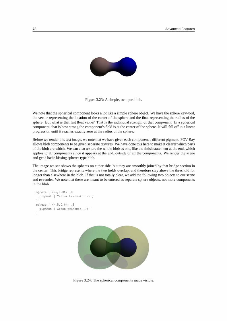
78 Advanced Features
Figure 3.23: A simple, two-part blob.
We note that the spherical component looks a lot like a simple sphere object. We have the sphere keyword,the vector representing the location of the center of the sphere and the float representing the radius of thesphere. But what is that last float value? That is the individual strength of that component. In a sphericalcomponent, that is how strong the component’s field is at the center of the sphere. It will fall off in a linearprogression until it reaches exactly zero at the radius of the sphere.
Before we render this test image, we note that we have given each component a different pigment. POV-Rayallows blob components to be given separate textures. We have done this here to make it clearer which partsof the blob are which. We can also texture the whole blob as one, like the finish statement at the end, whichapplies to all components since it appears at the end, outside of all the components. We render the sceneand get a basic kissing spheres type blob.
The image we see shows the spheres on either side, but they are smoothly joined by that bridge section inthe center. This bridge represents where the two fields overlap, and therefore stay above the threshold forlonger than elsewhere in the blob. If that is not totally clear, we add the following two objects to our sceneand re-render. We note that these are meant to be entered as separate sphere objects, not more componentsin the blob.
sphere { <.5,0,0>, .8pigment { Yellow transmit .75 }
}sphere { <-.5,0,0>, .8
pigment { Green transmit .75 }}
Figure 3.24: The spherical components made visible.
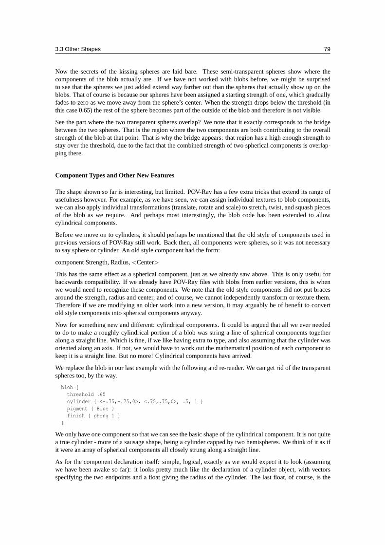
3.3 Other Shapes 79
Now the secrets of the kissing spheres are laid bare. These semi-transparent spheres show where thecomponents of the blob actually are. If we have not worked with blobs before, we might be surprisedto see that the spheres we just added extend way farther out than the spheres that actually show up on theblobs. That of course is because our spheres have been assigned a starting strength of one, which graduallyfades to zero as we move away from the sphere’s center. When the strength drops below the threshold (inthis case 0.65) the rest of the sphere becomes part of the outside of the blob and therefore is not visible.
See the part where the two transparent spheres overlap? We note that it exactly corresponds to the bridgebetween the two spheres. That is the region where the two components are both contributing to the overallstrength of the blob at that point. That is why the bridge appears: that region has a high enough strength tostay over the threshold, due to the fact that the combined strength of two spherical components is overlap-ping there.
Component Types and Other New Features
The shape shown so far is interesting, but limited. POV-Ray has a few extra tricks that extend its range ofusefulness however. For example, as we have seen, we can assign individual textures to blob components,we can also apply individual transformations (translate, rotate and scale) to stretch, twist, and squash piecesof the blob as we require. And perhaps most interestingly, the blob code has been extended to allowcylindrical components.
Before we move on to cylinders, it should perhaps be mentioned that the old style of components used inprevious versions of POV-Ray still work. Back then, all components were spheres, so it was not necessaryto say sphere or cylinder. An old style component had the form:
component Strength, Radius,<Center>
This has the same effect as a spherical component, just as we already saw above. This is only useful forbackwards compatibility. If we already have POV-Ray files with blobs from earlier versions, this is whenwe would need to recognize these components. We note that the old style components did not put bracesaround the strength, radius and center, and of course, we cannot independently transform or texture them.Therefore if we are modifying an older work into a new version, it may arguably be of benefit to convertold style components into spherical components anyway.
Now for something new and different: cylindrical components. It could be argued that all we ever neededto do to make a roughly cylindrical portion of a blob was string a line of spherical components togetheralong a straight line. Which is fine, if we like having extra to type, and also assuming that the cylinder wasoriented along an axis. If not, we would have to work out the mathematical position of each component tokeep it is a straight line. But no more! Cylindrical components have arrived.
We replace the blob in our last example with the following and re-render. We can get rid of the transparentspheres too, by the way.
blob {threshold .65cylinder { <-.75,-.75,0>, <.75,.75,0>, .5, 1 }pigment { Blue }finish { phong 1 }
}
We only have one component so that we can see the basic shape of the cylindrical component. It is not quitea true cylinder - more of a sausage shape, being a cylinder capped by two hemispheres. We think of it as ifit were an array of spherical components all closely strung along a straight line.
As for the component declaration itself: simple, logical, exactly as we would expect it to look (assumingwe have been awake so far): it looks pretty much like the declaration of a cylinder object, with vectorsspecifying the two endpoints and a float giving the radius of the cylinder. The last float, of course, is the
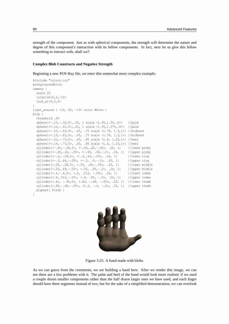
80 Advanced Features
strength of the component. Just as with spherical components, the strength will determine the nature anddegree of this component’s interaction with its fellow components. In fact, next let us give this fellowsomething to interact with, shall we?
Complex Blob Constructs and Negative Strength
Beginning a new POV-Ray file, we enter this somewhat more complex example:
#include "colors.inc"background{White}camera {
angle 20location<0,2,-10>look_at<0,0,0>
}light_source { <10, 20, -10> color White }blob {
threshold .65sphere{<-.23,-.32,0>,.43, 1 scale <1.95,1.05,.8>} //palmsphere{<+.12,-.41,0>,.43, 1 scale <1.95,1.075,.8>} //palmsphere{<-.23,-.63,0>, .45, .75 scale <1.78, 1.3,1>} //midhandsphere{<+.19,-.63,0>, .45, .75 scale <1.78, 1.3,1>} //midhandsphere{<-.22,-.73,0>, .45, .85 scale <1.4, 1.25,1>} //heelsphere{<+.19,-.73,0>, .45, .85 scale <1.4, 1.25,1>} //heelcylinder{<-.65,-.28,0>, <-.65,.28,-.05>, .26, 1} //lower pinkycylinder{<-.65,.28,-.05>, <-.65, .68,-.2>, .26, 1} //upper pinkycylinder{<-.3,-.28,0>, <-.3,.44,-.05>, .26, 1} //lower ringcylinder{<-.3,.44,-.05>, <-.3, .9,-.2>, .26, 1} //upper ringcylinder{<.05,-.28,0>, <.05, .49,-.05>, .26, 1} //lower middlecylinder{<.05,.49,-.05>, <.05, .95,-.2>, .26, 1} //upper middlecylinder{<.4,-.4,0>, <.4, .512, -.05>, .26, 1} //lower indexcylinder{<.4,.512,-.05>, <.4, .85, -.2>, .26, 1} //upper indexcylinder{<.41, -.95,0>, <.85, -.68, -.05>, .25, 1} //lower thumbcylinder{<.85,-.68,-.05>, <1.2, -.4, -.2>, .25, 1} //upper thumbpigment{ Flesh }
}
Figure 3.25: A hand made with blobs.
As we can guess from the comments, we are building a hand here. After we render this image, we cansee there are a few problems with it. The palm and heel of the hand would look more realistic if we useda couple dozen smaller components rather than the half dozen larger ones we have used, and each fingershould have three segments instead of two, but for the sake of a simplified demonstration, we can overlook
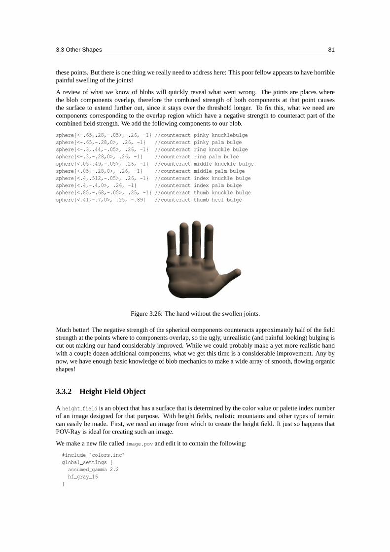
3.3 Other Shapes 81
these points. But there is one thing we really need to address here: This poor fellow appears to have horriblepainful swelling of the joints!
A review of what we know of blobs will quickly reveal what went wrong. The joints are places wherethe blob components overlap, therefore the combined strength of both components at that point causesthe surface to extend further out, since it stays over the threshold longer. To fix this, what we need arecomponents corresponding to the overlap region which have a negative strength to counteract part of thecombined field strength. We add the following components to our blob.
sphere{<-.65,.28,-.05>, .26, -1} //counteract pinky knucklebulgesphere{<-.65,-.28,0>, .26, -1} //counteract pinky palm bulgesphere{<-.3,.44,-.05>, .26, -1} //counteract ring knuckle bulgesphere{<-.3,-.28,0>, .26, -1} //counteract ring palm bulgesphere{<.05,.49,-.05>, .26, -1} //counteract middle knuckle bulgesphere{<.05,-.28,0>, .26, -1} //counteract middle palm bulgesphere{<.4,.512,-.05>, .26, -1} //counteract index knuckle bulgesphere{<.4,-.4,0>, .26, -1} //counteract index palm bulgesphere{<.85,-.68,-.05>, .25, -1} //counteract thumb knuckle bulgesphere{<.41,-.7,0>, .25, -.89} //counteract thumb heel bulge
Figure 3.26: The hand without the swollen joints.
Much better! The negative strength of the spherical components counteracts approximately half of the fieldstrength at the points where to components overlap, so the ugly, unrealistic (and painful looking) bulging iscut out making our hand considerably improved. While we could probably make a yet more realistic handwith a couple dozen additional components, what we get this time is a considerable improvement. Any bynow, we have enough basic knowledge of blob mechanics to make a wide array of smooth, flowing organicshapes!
3.3.2 Height Field Object
A height field is an object that has a surface that is determined by the color value or palette index numberof an image designed for that purpose. With height fields, realistic mountains and other types of terraincan easily be made. First, we need an image from which to create the height field. It just so happens thatPOV-Ray is ideal for creating such an image.
We make a new file calledimage.pov and edit it to contain the following:
#include "colors.inc"global_settings {
assumed_gamma 2.2hf_gray_16
}
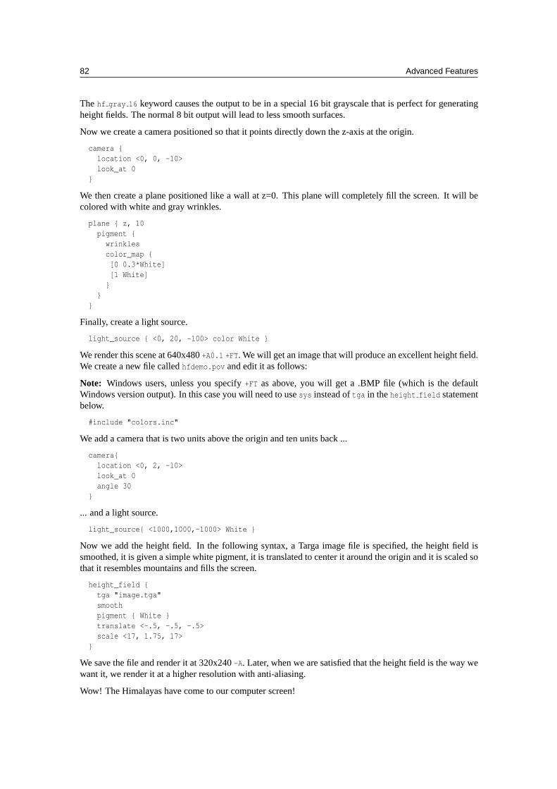
82 Advanced Features
Thehf gray 16 keyword causes the output to be in a special 16 bit grayscale that is perfect for generatingheight fields. The normal 8 bit output will lead to less smooth surfaces.
Now we create a camera positioned so that it points directly down the z-axis at the origin.
camera {location <0, 0, -10>look_at 0
}
We then create a plane positioned like a wall at z=0. This plane will completely fill the screen. It will becolored with white and gray wrinkles.
plane { z, 10pigment {
wrinklescolor_map {[0 0.3*White][1 White]
}}
}
Finally, create a light source.
light_source { <0, 20, -100> color White }
We render this scene at 640x480+A0.1 +FT. We will get an image that will produce an excellent height field.We create a new file calledhfdemo.pov and edit it as follows:
Note: Windows users, unless you specify+FT as above, you will get a .BMP file (which is the defaultWindows version output). In this case you will need to usesys instead oftga in theheight field statementbelow.
#include "colors.inc"
We add a camera that is two units above the origin and ten units back ...
camera{location <0, 2, -10>look_at 0angle 30
}
... and a light source.
light_source{ <1000,1000,-1000> White }
Now we add the height field. In the following syntax, a Targa image file is specified, the height field issmoothed, it is given a simple white pigment, it is translated to center it around the origin and it is scaled sothat it resembles mountains and fills the screen.
height_field {tga "image.tga"smoothpigment { White }translate <-.5, -.5, -.5>scale <17, 1.75, 17>
}
We save the file and render it at 320x240-A. Later, when we are satisfied that the height field is the way wewant it, we render it at a higher resolution with anti-aliasing.
Wow! The Himalayas have come to our computer screen!
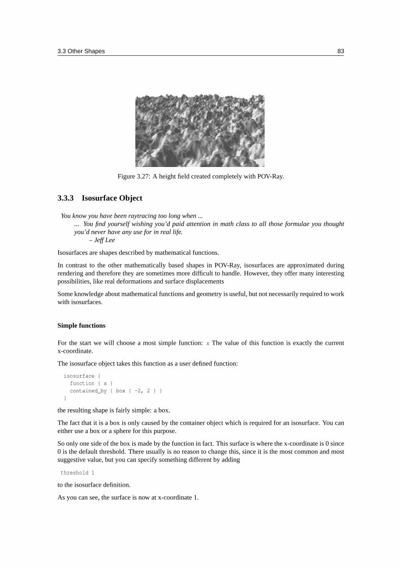
3.3 Other Shapes 83
Figure 3.27: A height field created completely with POV-Ray.
3.3.3 Isosurface Object
You know you have been raytracing too long when ...... You find yourself wishing you’d paid attention in math class to all those formulae you thoughtyou’d never have any use for in real life.
– Jeff Lee
Isosurfaces are shapes described by mathematical functions.
In contrast to the other mathematically based shapes in POV-Ray, isosurfaces are approximated duringrendering and therefore they are sometimes more difficult to handle. However, they offer many interestingpossibilities, like real deformations and surface displacements
Some knowledge about mathematical functions and geometry is useful, but not necessarily required to workwith isosurfaces.
Simple functions
For the start we will choose a most simple function:x The value of this function is exactly the currentx-coordinate.
The isosurface object takes this function as a user defined function:
isosurface {function { x }contained_by { box { -2, 2 } }
}
the resulting shape is fairly simple: a box.
The fact that it is a box is only caused by the container object which is required for an isosurface. You caneither use a box or a sphere for this purpose.
So only one side of the box is made by the function in fact. This surface is where the x-coordinate is 0 since0 is the default threshold. There usually is no reason to change this, since it is the most common and mostsuggestive value, but you can specify something different by adding
threshold 1
to the isosurface definition.
As you can see, the surface is now at x-coordinate 1.
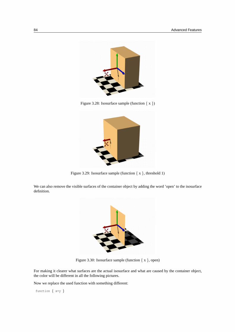
84 Advanced Features
Figure 3.28: Isosurface sample (function{ x })
Figure 3.29: Isosurface sample (function{ x }, threshold 1)
We can also remove the visible surfaces of the container object by adding the word ’open’ to the isosurfacedefinition.
Figure 3.30: Isosurface sample (function{ x }, open)
For making it clearer what surfaces are the actual isosurface and what are caused by the container object,the color will be different in all the following pictures.
Now we replace the used function with something different:
function { x+y }
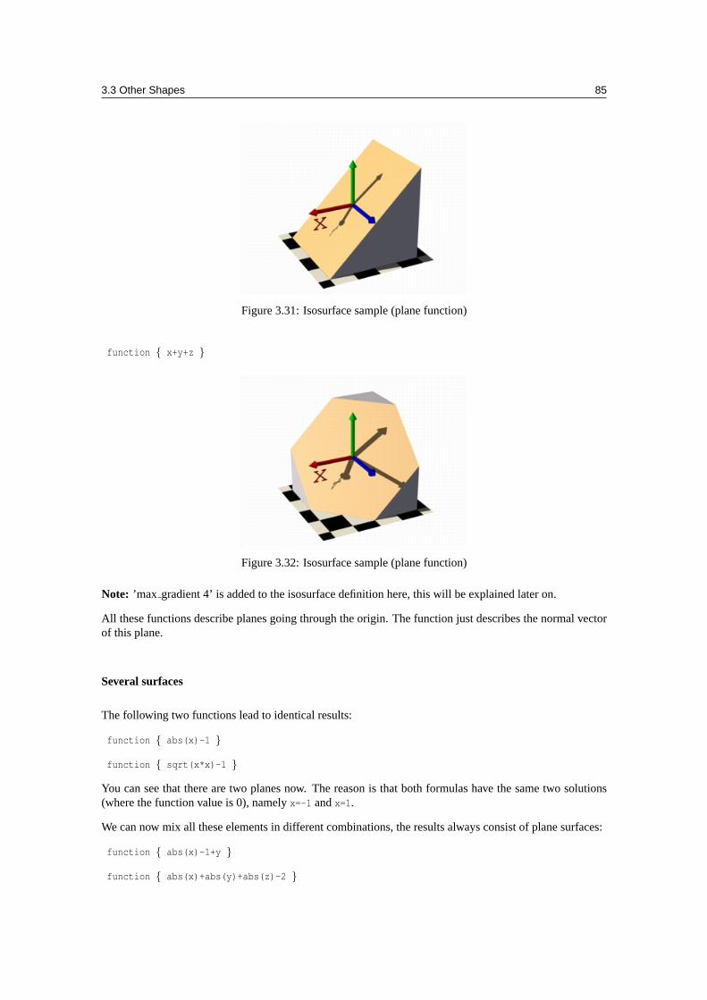
3.3 Other Shapes 85
Figure 3.31: Isosurface sample (plane function)
function { x+y+z }
Figure 3.32: Isosurface sample (plane function)
Note: ’max gradient 4’ is added to the isosurface definition here, this will be explained later on.
All these functions describe planes going through the origin. The function just describes the normal vectorof this plane.
Several surfaces
The following two functions lead to identical results:
function { abs(x)-1 }
function { sqrt(x*x)-1 }
You can see that there are two planes now. The reason is that both formulas have the same two solutions(where the function value is 0), namelyx=-1 andx=1.
We can now mix all these elements in different combinations, the results always consist of plane surfaces:
function { abs(x)-1+y }
function { abs(x)+abs(y)+abs(z)-2 }
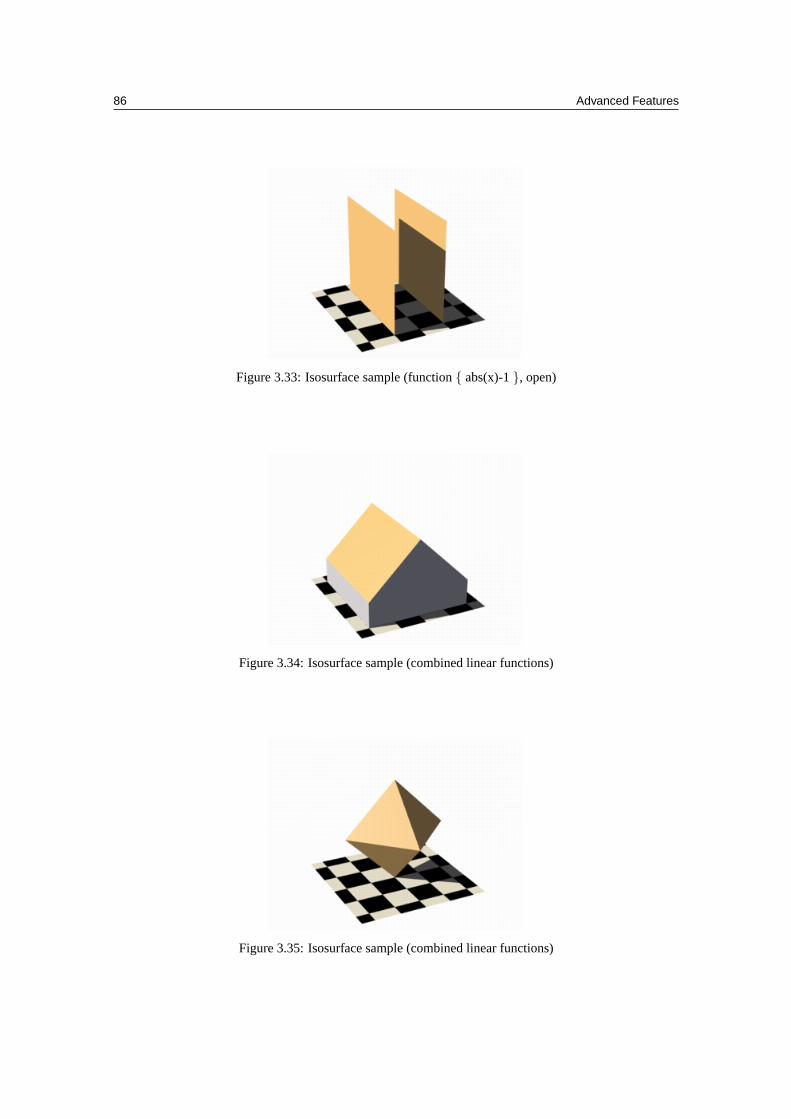
86 Advanced Features
Figure 3.33: Isosurface sample (function{ abs(x)-1}, open)
Figure 3.34: Isosurface sample (combined linear functions)
Figure 3.35: Isosurface sample (combined linear functions)
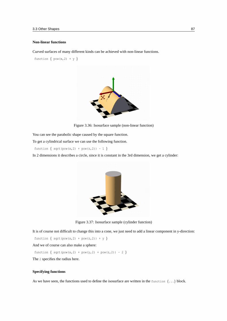
3.3 Other Shapes 87
Non-linear functions
Curved surfaces of many different kinds can be achieved with non-linear functions.
function { pow(x,2) + y }
Figure 3.36: Isosurface sample (non-linear function)
You can see the parabolic shape caused by the square function.
To get a cylindrical surface we can use the following function.
function { sqrt(pow(x,2) + pow(z,2)) - 1 }
In 2 dimensions it describes a circle, since it is constant in the 3rd dimension, we get a cylinder:
Figure 3.37: Isosurface sample (cylinder function)
It is of course not difficult to change this into a cone, we just need to add a linear component in y-direction:
function { sqrt(pow(x,2) + pow(z,2)) + y }
And we of course can also make a sphere:
function { sqrt(pow(x,2) + pow(y,2) + pow(z,2)) - 2 }
The2 specifies the radius here.
Specifying functions
As we have seen, the functions used to define the isosurface are written in thefunction {...} block.
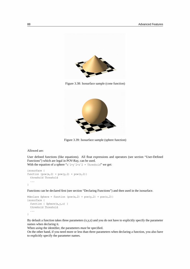
88 Advanced Features
Figure 3.38: Isosurface sample (cone function)
Figure 3.39: Isosurface sample (sphere function)
Allowed are:
User defined functions (like equations). All float expressions and operators (see section “User-DefinedFunctions”) which are legal in POV-Ray, can be used.With the equation of a sphere “xˆ2+yˆ2+zˆ2 = Threshold” we get:
isosurface {function {pow(x,2) + pow(y,2) + pow(z,2)}
threshold Threshold...
}
Functions can be declared first (see section “Declaring Functions”) and then used in the isosurface.
#declare Sphere = function {pow(x,2) + pow(y,2) + pow(z,2)}isosurface {
function { Sphere(x,y,z) }threshold Threshold...
}
By default a function takes three parameters (x,y,z) and you do not have to explicitly specify the parameternames when declaring it.Whenusingthe identifier, the parametersmustbe specified.On the other hand, if you need more or less than three parameters when declaring a function, you also haveto explicitly specify the parameter names.
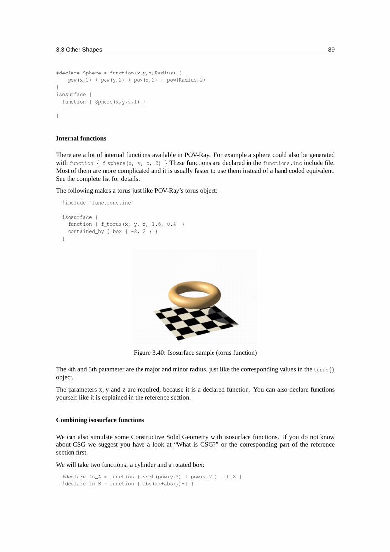
3.3 Other Shapes 89
#declare Sphere = function(x,y,z,Radius) {pow(x,2) + pow(y,2) + pow(z,2) - pow(Radius,2)
}isosurface {
function { Sphere(x,y,z,1) }...
}
Internal functions
There are a lot of internal functions available in POV-Ray. For example a sphere could also be generatedwith function { f sphere(x, y, z, 2) } These functions are declared in thefunctions.inc include file.Most of them are more complicated and it is usually faster to use them instead of a hand coded equivalent.See the complete list for details.
The following makes a torus just like POV-Ray’s torus object:
#include "functions.inc"
isosurface {function { f_torus(x, y, z, 1.6, 0.4) }contained_by { box { -2, 2 } }
}
Figure 3.40: Isosurface sample (torus function)
The 4th and 5th parameter are the major and minor radius, just like the corresponding values in thetorus{}object.
The parameters x, y and z are required, because it is a declared function. You can also declare functionsyourself like it is explained in the reference section.
Combining isosurface functions
We can also simulate some Constructive Solid Geometry with isosurface functions. If you do not knowabout CSG we suggest you have a look at “What is CSG?” or the corresponding part of the referencesection first.
We will take two functions: a cylinder and a rotated box:
#declare fn_A = function { sqrt(pow(y,2) + pow(z,2)) - 0.8 }#declare fn_B = function { abs(x)+abs(y)-1 }
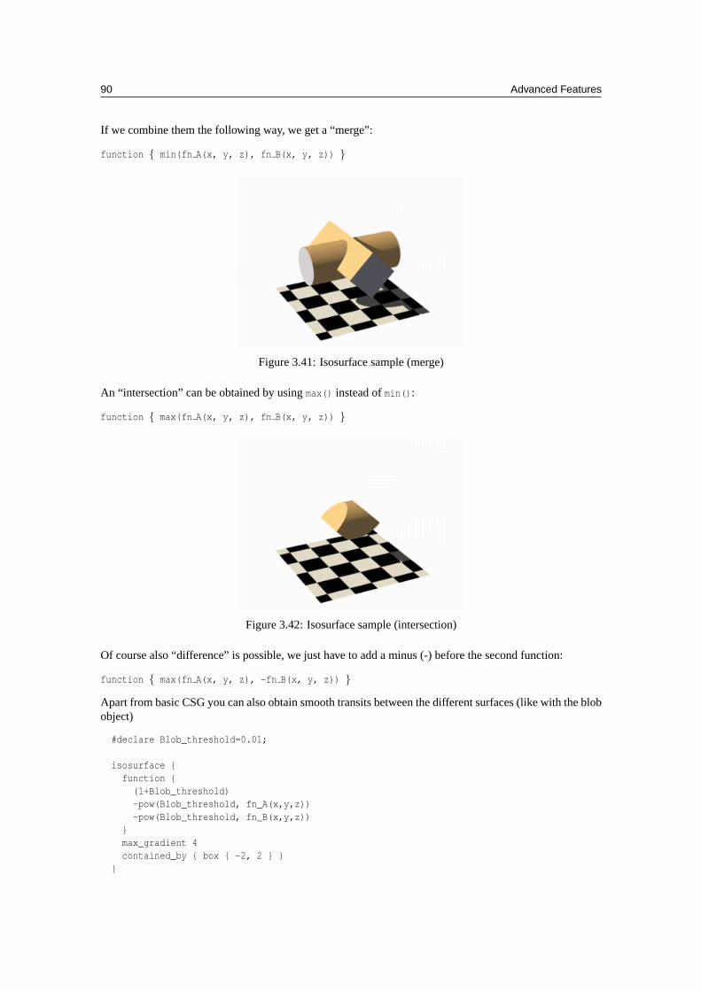
90 Advanced Features
If we combine them the following way, we get a “merge”:
function { min(fn A(x, y, z), fn B(x, y, z)) }
Figure 3.41: Isosurface sample (merge)
An “intersection” can be obtained by usingmax() instead ofmin():
function { max(fn A(x, y, z), fn B(x, y, z)) }
Figure 3.42: Isosurface sample (intersection)
Of course also “difference” is possible, we just have to add a minus (-) before the second function:
function { max(fn A(x, y, z), -fn B(x, y, z)) }
Apart from basic CSG you can also obtain smooth transits between the different surfaces (like with the blobobject)
#declare Blob_threshold=0.01;
isosurface {function {
(1+Blob_threshold)-pow(Blob_threshold, fn_A(x,y,z))-pow(Blob_threshold, fn_B(x,y,z))
}max_gradient 4contained_by { box { -2, 2 } }
}
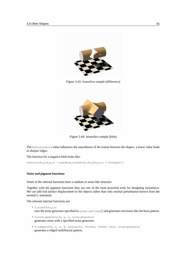
3.3 Other Shapes 91
Figure 3.43: Isosurface sample (difference)
Figure 3.44: Isosurface sample (blob)
TheBlob threshold value influences the smoothness of the transit between the shapes. a lower value leadsto sharper edges.
The function for a negative blob looks like:
function{fn_A(x,y,z) + pow(Blob_threshold,(Fn_B(x,y,z) + Strength))}
Noise and pigment functions
Some of the internal functions have a random or noise-like structure
Together with the pigment functions they are one of the most powerful tools for designing isosurfaces.We can add real surface displacement to the objects rather than only normal perturbation known from thenormal{} statement.
The relevant internal functions are:
• f noise3d(x,y,z)
uses the noise generator specified inglobal settings{} and generates structures like the bozo pattern.
• f noise generator(x, y, z, noise generator)
generates noise with a specified noise generator.
• f ridged mf(x, y, z, H, Lacunarity, Octaves, Offset, Gain, noise generator)
generates a ridged multifractal pattern.
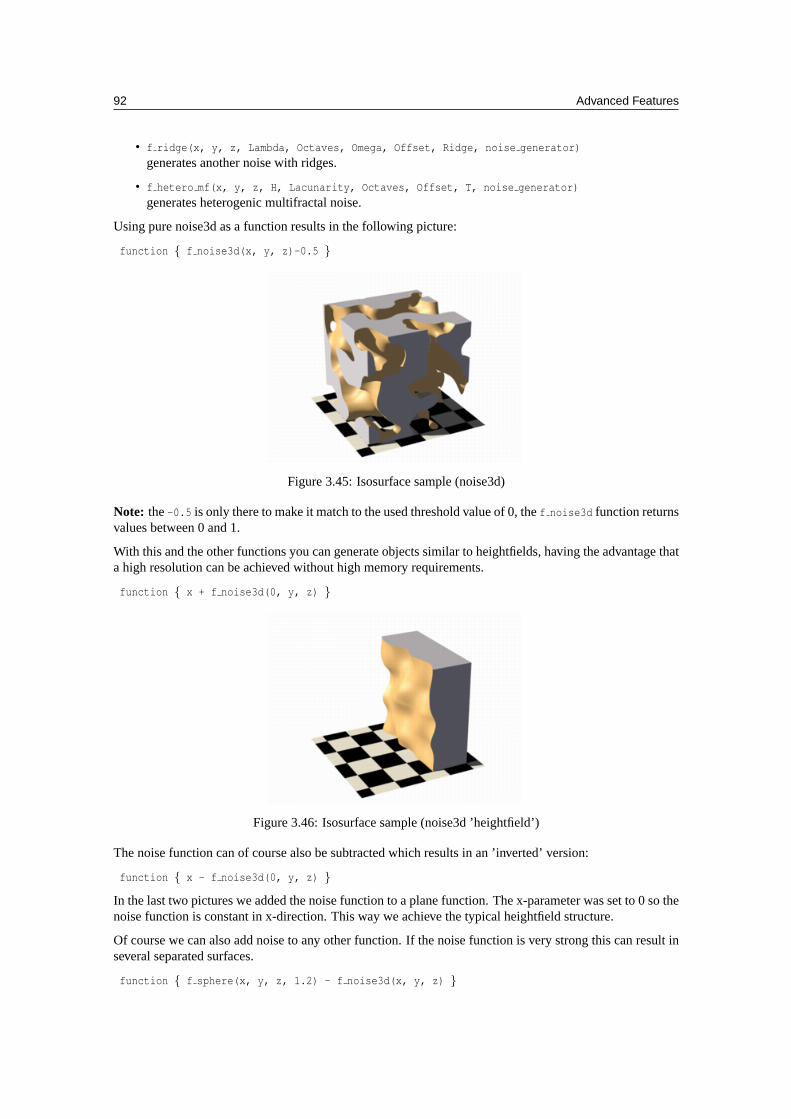
92 Advanced Features
• f ridge(x, y, z, Lambda, Octaves, Omega, Offset, Ridge, noise generator)
generates another noise with ridges.
• f hetero mf(x, y, z, H, Lacunarity, Octaves, Offset, T, noise generator)
generates heterogenic multifractal noise.
Using pure noise3d as a function results in the following picture:
function { f noise3d(x, y, z)-0.5 }
Figure 3.45: Isosurface sample (noise3d)
Note: the-0.5 is only there to make it match to the used threshold value of 0, thef noise3d function returnsvalues between 0 and 1.
With this and the other functions you can generate objects similar to heightfields, having the advantage thata high resolution can be achieved without high memory requirements.
function { x + f noise3d(0, y, z) }
Figure 3.46: Isosurface sample (noise3d ’heightfield’)
The noise function can of course also be subtracted which results in an ’inverted’ version:
function { x - f noise3d(0, y, z) }
In the last two pictures we added the noise function to a plane function. The x-parameter was set to 0 so thenoise function is constant in x-direction. This way we achieve the typical heightfield structure.
Of course we can also add noise to any other function. If the noise function is very strong this can result inseveral separated surfaces.
function { f sphere(x, y, z, 1.2) - f noise3d(x, y, z) }
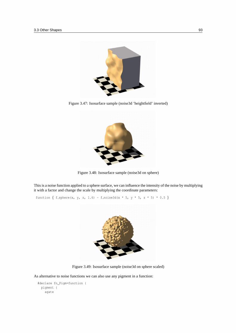
3.3 Other Shapes 93
Figure 3.47: Isosurface sample (noise3d ’heightfield’ inverted)
Figure 3.48: Isosurface sample (noise3d on sphere)
This is a noise function applied to a sphere surface, we can influence the intensity of the noise by multiplyingit with a factor and change the scale by multiplying the coordinate parameters:
function { f sphere(x, y, z, 1.6) - f noise3d(x * 5, y * 5, z * 5) * 0.5 }
Figure 3.49: Isosurface sample (noise3d on sphere scaled)
As alternative to noise functions we can also use any pigment in a function:
#declare fn_Pigm=function {pigment {
agate
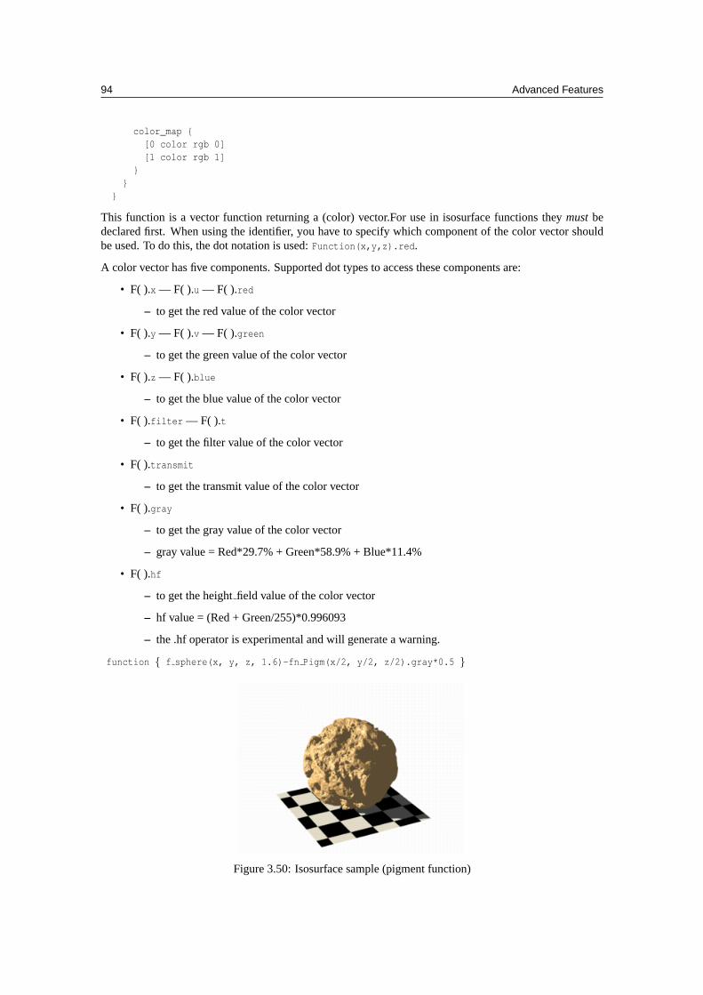
94 Advanced Features
color_map {[0 color rgb 0][1 color rgb 1]
}}
}
This function is a vector function returning a (color) vector.For use in isosurface functions theymustbedeclared first. When using the identifier, you have to specify which component of the color vector shouldbe used. To do this, the dot notation is used:Function(x,y,z).red.
A color vector has five components. Supported dot types to access these components are:
• F( ).x — F( ).u — F( ).red
– to get the red value of the color vector
• F( ).y — F( ).v — F( ).green
– to get the green value of the color vector
• F( ).z — F( ).blue
– to get the blue value of the color vector
• F( ).filter — F( ).t
– to get the filter value of the color vector
• F( ).transmit
– to get the transmit value of the color vector
• F( ).gray
– to get the gray value of the color vector
– gray value = Red*29.7% + Green*58.9% + Blue*11.4%
• F( ).hf
– to get the heightfield value of the color vector
– hf value = (Red + Green/255)*0.996093
– the .hf operator is experimental and will generate a warning.
function { f sphere(x, y, z, 1.6)-fn Pigm(x/2, y/2, z/2).gray*0.5 }
Figure 3.50: Isosurface sample (pigment function)
3.3 Other Shapes 95
There are quite a lot of things possible with pigment functions, but you probably have recognized that thisrenders quite slow.
Conditional directives and loops
Conditional directives are allowed in functions:
#declare Rough = yes;#include "functions.inc"isosurface {
function { y #if(Rough=1)-f_noise3d(x/0.5,y/0.3,z/0.4)*0.8 #end }...
}
Loops can also be used in functions:
#include "functions.inc"#declare Thr = 1/1000;#declare Ang = radians(45);#declare Offset = 1.5;#declare Scale = 1.2;#declare TrSph = function { f_sphere(x-Offset,y,z,0.7*Scale) }
function {(1-Thr)#declare A = 0;#while (A<8)-pow(Thr, TrSph(x*cos(A*Ang) + y*sin(A*Ang),
y*cos(A*Ang) -x*sin(A*Ang), z) )#declare A=A+1;
#end}
Note: The loops and conditionals are evaluated at parse time, not at render time.
Transformations on functions
Transforming an isosurface object is done like transforming any POV-Ray object. Simply use the objectmodifiers (scale, translate, rotate, ...).
However, when you want to transform functions within the containedby object, you have to substituteparameters in the functions.
The resultsseeminverted to what you would normally expect. Here is an explanation:Take a Sphere(x,y,z). We know it sits at the origin because x=0. When we want it at x=2 (translating 2 unitsto the right) we need to write the second equation in the same form: x-2=0Now that both equations equal 0, we can replace parameter x with x-2So our Sphere(x-2, y,z) moves two units to theright.
Let’s scale our Sphere 0.5 in the y direction. Default size is y=1 (one unit). We want y=0.5.To get this equation in the same form as the first one, we have to multiply both sides by two. y*2 = 0.5*2,which gives y*2=1Now we can replace the y parameter in our sphere: Sphere(x, y*2, z). This squishes the y-size of the sphereby half.Well, this is the general idea of substitutions.
96 Advanced Features
Here is an overview of some useful substitutions:Using a declared object P(x,y,z)
Scalescale x : replace “x” with “ x/scale” (idem other parameters)
scale x*2 gives P(x/2,y,z)
Scale Infinitelyscale x infinitely : replace ”x” with ” 0” (idem other parameters)
scale y infinitely gives P(x,0,z)
Translatetranslate x : replace ”x” with ” x - translation” (idem other parameters)
translate z*3 gives P(x,y,z-3)
Shearshear in XY-plane : replace ”x” with ” x + y*tan(radians(Angle))” (idem other parameters)
shear 45 degrees left gives P(x+y*tan(radians(45)), y, z)
Rotate
Note: these rotation substitutions work like normal POV-rotations: they already compensate for the inverseworking
rotate around X: replace ”y” with ” z*sin(radians(Angle)) + y*cos(radians(Angle))”: replace ”z” with ” z*cos(radians(Angle)) - y*sin(radians(Angle))”
rotate around Y: replace ”x” with ” x*cos(radians(Angle)) - z*sin(radians(Angle))”: replace ”z” with ” x*sin(radians(Angle)) + z*cos(radians(Angle))”
rotate around Z: replace ”x” with ” x*cos(radians(Angle)) + y*sin(radians(Angle))”: replace ”y” with ” -x*sin(radians(Angle)) + y*cos(radians(Angle)) ”
rotate z*75 gives:P(x*cos(radians(75)) + y*sin(radians(75)),
-x*sin(radians(75)) + y*cos(radians(75)), z)
Flipflip X - Y : replace ”x” with ” y” and replace ”y” with ” -x”
flip Y - Z : replace ”y” with ” z” and replace ”z” with ” -y”
flip X - Z : replace ”x” with ” -z” and replace ”z” with ” x”
flip x and y gives P(y, -x, z)
Twisttwist N turns/unit aroundX: replace ”y” with ” z*sin(x*2*pi*N) + y*cos(x*2*pi*N)”: replace ”z” with ” z*cos(x*2*pi*N) - y*sin(x*2*pi*N)”
3.3 Other Shapes 97
Improving Isosurface Speed
To optimize the approximation of the isosurface and to get maximum rendering speed it is important toadapt certain values;
accuracy
The accuracy value influences how accurate the surface geometry is calculated. Lower values lead to a moreprecise, but slower result. The default value of0.001 is fairly low. We used this value in all the previoussamples, but often you can raise this quite a lot and thereby make things faster.
max gradient
For finding the actual surface it is important for POV-Ray to know the maximum gradient of the function,meaning how fast the function value changes. We can specify a value with themax gradient keyword.Lower maxgradient values lead to faster rendering, but if the specified value is below the actual maximumgradient of the function, there can be holes or other artefacts in the surface.
For the same reason functions with infinite gradient should not be used. This applies for pigment functionswith brick or checker pattern for example. You should also be careful when usingselect() in isosurfacefunctions because of this.
If the real maximum gradient differs too much from the specified value POV-Ray prints a warning togetherwith the found maximum gradient. It is usually sufficient to use this number for themax gradient parameterto get fast and correct results.
POV-Ray can also dynamically change themax gradient when you specifyevaluate with 3 parametersthe isosurface definition. Concerning the details on this and other things see the evaluate in the referencesection.
contained by
Make sure yourcontained by ’object’ fits as tightly as possible. An oversized container can sky-rocket therender time.When the container has a lot of empty space around the actual isosurface, POV-Ray has to do a lot ofsuperfluous sampling: especially with complex functions this can become very time consuming. On top ofthis, themax gradient needed to get a proper surface will also increase rapidly (almost proportional to theoversize!).You could use a transparent copy of the container (using exactly the same transformations) to check how itfits. Getting themin extent andmax extent of theisosurface is not useful because it only gives the extentof the container and not of the actual isosurface.
3.3.4 Poly Object
The polynomial object (and its ”shortcut” versions:cubic, quartic andquadric) of POV-Ray is one ofthe most complex and mathematical primitives of the program. One could think that it is seldom used andmore or less obsolete, but we have to remember that for example the torus primitive is just a shortcut for theequivalentquartic, which is just a shortcut for the equivalentpoly object. Polys are, however, seldom usedin scenes due to the fact that they are so difficult to define and it is far from trivial to get the desired shapewith just a polynomial equation. It is mostly used by the most mathematically oriented POV-Ray users.
This tutorial explains the process of making a polynomial object in POV-Ray.
Note:Since version 3.5, POV-Ray includes the newisosurface object which makes the polynomial objectmore or less obsolete. The isosurface is more versatile (you can specify any mathematical function, not justpolynomials), easier to use. You can write the function as is, without needing to put values in a giganticvector. Isosurfaces often render considerably faster than equivalent polys.
98 Advanced Features
However, the most mathematically oriented still like polys because isosurfaces are calculated just by ap-proximating the right value, while the poly is calculated in a mathematically exact way. Usually isosurfacesare more than good enough for most applications, though.
Note: at maximum a 15th degree polynomial can be represented with the poly object. If a higher degreepolynomial or other non-polynomial function has to be represented, then it is necessary to use the isosurfaceobject.
Creating the polynomial function
The first step is to create the polynomial function to be represented. You will need some (high-school level)mathematical knowledge for this.
1) Let’s start with an easy example: A sphere.
The sphere function is:
√x2 +y2 +z2 = r
Equation 3.1: sphere function
Now we have to convert this to polynomial form:
x2 +y2 +z2− r = 0
Equation 3.2: sphere polynomial
We will need a polynomial of the 2nd degree to represent this.
2) A more elaborated example:
Let’s take the function:
z=2xy2
x2 +y4
Equation 3.3: function
Converting this to polynomial form we get:
Although the highest power is 4 we will need a 5th order polynomial to represent this function (because wecannot represent y4z with a 4th order polynomial).
3) And since we talked about the torus, let’s also take it as an example.
A torus can be represented with the function:
where r1 is the major radius and r2 is the minor radius.
Now, this is tougher to convert to polynomial form, but finally we get:
A 4th order polynomial is enough to represent this.
3.3 Other Shapes 99
x2z+y4z−2xy2 = 0
Equation 3.4: polynomial
√( √x2 +z2− r1
)2+y2 = r2
Equation 3.5: torus function
Note: not every function can be represented in polynomial form. Only functions that use addition (andsubstraction), multiplication (and division) and scalar powers (including rational powers, eg. the squareroot) can be represented. Also, the poly primitive supports only polynomials of the 7th degree at max.
Converting a function to polynomial form may be a very laborious task for certain functions. Some mathe-matical programs are very helpful in this matter.
Writing the polynomial vector
Now that we have the function in polynomial form, we have to write it in POV-Ray syntax. The syntax isspecified in the in the chapters ”Poly, Cubic and Quartic” and ”Quadric” of the SDL section. There is alsoa table in this chapter which we will be using to make the polynomial vector. It is easier to have this tableprinted on paper.
Note: It is also possible to make a little program with your favorite programming language which will printthe poly vector from the polynomial function, but making a program like this is up to you.
1) Let’s start with the easy one, ie. the sphere.
Since the sphere can be represented with a polynomial of 2nd degree, we look at the row titled ”2nd” in thetable. We see that it has 10 items, ie. we need a vector of size 10. Each item of the vector will be the factorof the term listed in the table.
The polynomial was:
Writing the poly in this way we get:
#declare Radius=1;poly{ 2,
<1,0,0,0,1,0,0,1,0,-Radius*Radius>
}
Put each group of factors (separated with lines in the table) in their own lines.
In the table we see that the first item is the factor for x2, which is 1 in the function. The next item is xy.Since it is not in the function, its factor is 0. Likewise the next item, which is xz. And so on. The last itemis the scalar term, which is in this case -r2.
x4 +2x2y2 +2x2z2−2(r21 + r2
2)x2 +y4 +2y2z2 +2(r2
1− r22)y
2 +z4−2(r21 + r2
2)z2 +(r2
1− r22)
2 = 0
Equation 3.6: torus polynomial
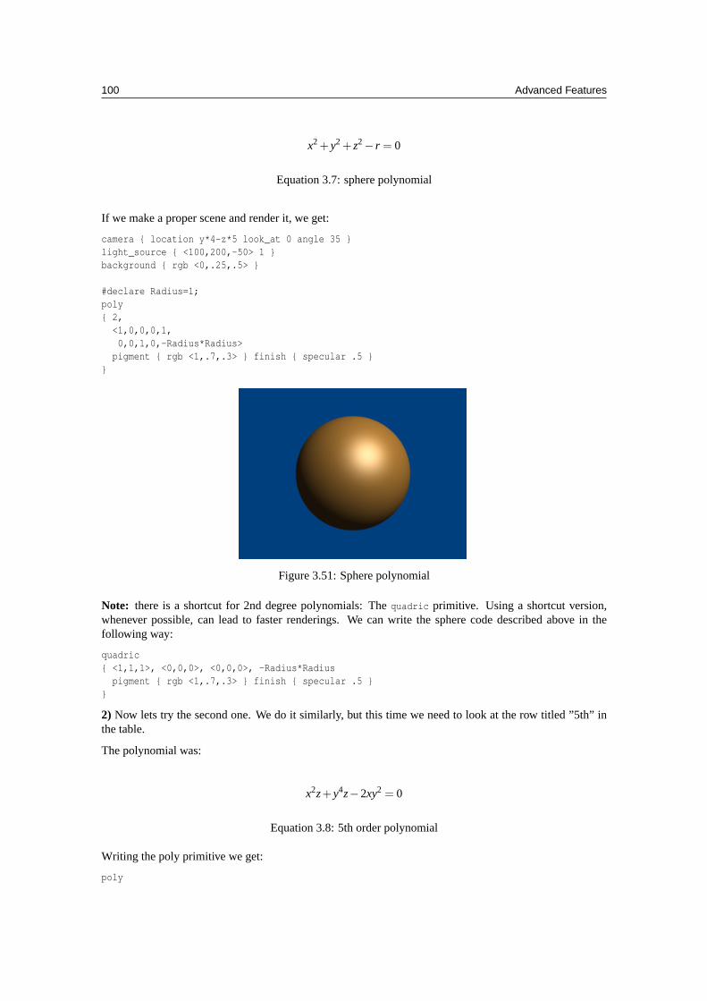
100 Advanced Features
x2 +y2 +z2− r = 0
Equation 3.7: sphere polynomial
If we make a proper scene and render it, we get:
camera { location y*4-z*5 look_at 0 angle 35 }light_source { <100,200,-50> 1 }background { rgb <0,.25,.5> }
#declare Radius=1;poly{ 2,
<1,0,0,0,1,0,0,1,0,-Radius*Radius>
pigment { rgb <1,.7,.3> } finish { specular .5 }}
Figure 3.51: Sphere polynomial
Note: there is a shortcut for 2nd degree polynomials: Thequadric primitive. Using a shortcut version,whenever possible, can lead to faster renderings. We can write the sphere code described above in thefollowing way:
quadric{ <1,1,1>, <0,0,0>, <0,0,0>, -Radius*Radius
pigment { rgb <1,.7,.3> } finish { specular .5 }}
2) Now lets try the second one. We do it similarly, but this time we need to look at the row titled ”5th” inthe table.
The polynomial was:
x2z+y4z−2xy2 = 0
Equation 3.8: 5th order polynomial
Writing the poly primitive we get:
poly
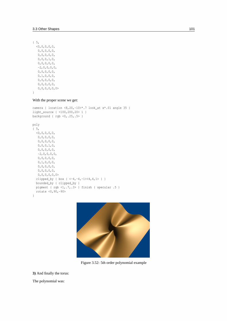
3.3 Other Shapes 101
{ 5,<0,0,0,0,0,0,0,0,0,0,0,0,0,0,0,0,0,0,1,0,0,0,0,0,0,-2,0,0,0,0,0,0,0,0,0,0,1,0,0,0,0,0,0,0,0,0,0,0,0,0,0,0,0,0,0,0>
}
With the proper scene we get:
camera { location <8,20,-10>*.7 look_at x*.01 angle 35 }light_source { <100,200,20> 1 }background { rgb <0,.25,.5> }
poly{ 5,
<0,0,0,0,0,0,0,0,0,0,0,0,0,0,0,0,0,0,1,0,0,0,0,0,0,-2,0,0,0,0,0,0,0,0,0,0,1,0,0,0,0,0,0,0,0,0,0,0,0,0,0,0,0,0,0,0>
clipped_by { box { <-4,-4,-1><4,4,1> } }bounded_by { clipped_by }pigment { rgb <1,.7,.3> } finish { specular .5 }rotate <0,90,-90>
}
Figure 3.52: 5th order polynomial example
3) And finally the torus:
The polynomial was:
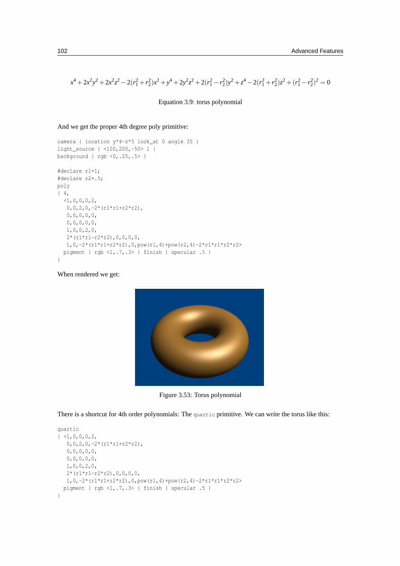
102 Advanced Features
x4 +2x2y2 +2x2z2−2(r21 + r2
2)x2 +y4 +2y2z2 +2(r2
1− r22)y
2 +z4−2(r21 + r2
2)z2 +(r2
1− r22)
2 = 0
Equation 3.9: torus polynomial
And we get the proper 4th degree poly primitive:
camera { location y*4-z*5 look_at 0 angle 35 }light_source { <100,200,-50> 1 }background { rgb <0,.25,.5> }
#declare r1=1;#declare r2=.5;poly{ 4,
<1,0,0,0,2,0,0,2,0,-2*(r1*r1+r2*r2),0,0,0,0,0,0,0,0,0,0,1,0,0,2,0,2*(r1*r1-r2*r2),0,0,0,0,1,0,-2*(r1*r1+r2*r2),0,pow(r1,4)+pow(r2,4)-2*r1*r1*r2*r2>
pigment { rgb <1,.7,.3> } finish { specular .5 }}
When rendered we get:
Figure 3.53: Torus polynomial
There is a shortcut for 4th order polynomials: Thequartic primitive. We can write the torus like this:
quartic{ <1,0,0,0,2,
0,0,2,0,-2*(r1*r1+r2*r2),0,0,0,0,0,0,0,0,0,0,1,0,0,2,0,2*(r1*r1-r2*r2),0,0,0,0,1,0,-2*(r1*r1+r2*r2),0,pow(r1,4)+pow(r2,4)-2*r1*r1*r2*r2>
pigment { rgb <1,.7,.3> } finish { specular .5 }}
3.3 Other Shapes 103
3.3.5 Superquadric Ellipsoid Object
Sometimes we want to make an object that does not have perfectly sharp edges like a box does. Then, thesuperquadric ellipsoid shape made by thesuperellipsoid is a useful object. It is described by the simplesyntax:
superellipsoid { <Value_E, Value_N >}
WhereValueE andValueN are float values greater than zero and less than or equal to one. Let’s make asuperellipsoid and experiment with the values ofValueE andValueN to see what kind of shapes we canmake. We create a file calledsupellps.pov and edit it as follows:
#include "colors.inc"camera {
location <10, 5, -20>look_at 0angle 15
}background { color rgb <.5, .5, .5> }light_source { <10, 50, -100> White }
The addition of a gray background makes it a little easier to see our object. We now type:
superellipsoid { <.25, .25>pigment { Red }
}
We save the file and trace it at 200x150-A to see the shape. It will look like a box, but the edges will berounded off. Now let’s experiment with different values ofValueE and ValueN. For the next trace, try<1,0.2>. The shape now looks like a cylinder, but the top edges are rounded. Now try<0.1, 1>. This shapeis an odd one! We do not know exactly what to call it, but it is interesting. Finally, let’s try<1, 1>. Well,this is more familiar... a sphere!
There are a couple of facts about superellipsoids we should know. First, we should not use a value of 0for either ValueE nor ValueN. This will cause POV-Ray to incorrectly make a black box instead of ourdesired shape. Second, very small values ofValueE and ValueN may yield strange results so they shouldbe avoided. Finally, the Sturmian root solver will not work with superellipsoids.
Superellipsoids are finite objects so they respond to auto-bounding and can be used in CSG.
Now let’s use the superellipsoid to make something that would be useful in a scene. We will make a tiledfloor and place a couple of superellipsoid objects hovering over it. We can start with the file we have alreadymade.
We rename it to tiles.pov and edit it so that it reads as follows:
#include "colors.inc"#include "textures.inc"camera {
location <10, 5, -20>look_at 0angle 15
}background { color rgb <.5, .5, .5> }light_source{ <10, 50, -100> White }
Note: we have added#include "textures.inc" so we can use pre-defined textures. Now we want to definethe superellipsoid which will be our tile.
#declare Tile = superellipsoid { <0.5, 0.1>scale <1, .05, 1>
104 Advanced Features
}
Superellipsoids are roughly 2*2*2 units unless we scale them otherwise. If we wish to lay a bunch of ourtiles side by side, they will have to be offset from each other so they do not overlap. We should select anoffset value that is slightly more than 2 so that we have some space between the tiles to fill with grout. Sowe now add this:
#declare Offset = 2.1;
We now want to lay down a row of tiles. Each tile will be offset from the original by an ever-increasingamount in both the +z and -z directions. We refer to our offset and multiply by the tile’s rank to determinethe position of each tile in the row. We also union these tiles into a single object calledRow like this:
#declare Row = union {object { Tile }object { Tile translate z*Offset }object { Tile translate z*Offset*2 }object { Tile translate z*Offset*3 }object { Tile translate z*Offset*4 }object { Tile translate z*Offset*5 }object { Tile translate z*Offset*6 }object { Tile translate z*Offset*7 }object { Tile translate z*Offset*8 }object { Tile translate z*Offset*9 }object { Tile translate z*Offset*10 }object { Tile translate -z*Offset }object { Tile translate -z*Offset*2 }object { Tile translate -z*Offset*3 }object { Tile translate -z*Offset*4 }object { Tile translate -z*Offset*5 }object { Tile translate -z*Offset*6 }
}
This gives us a single row of 17 tiles, more than enough to fill the screen. Now we must make copies of theRow and translate them, again by the offset value, in both the +x and -x directions in ever increasing amountsin the same manner.
object { Row }object { Row translate x*Offset }object { Row translate x*Offset*2 }object { Row translate x*Offset*3 }object { Row translate x*Offset*4 }object { Row translate x*Offset*5 }object { Row translate x*Offset*6 }object { Row translate x*Offset*7 }object { Row translate -x*Offset }object { Row translate -x*Offset*2 }object { Row translate -x*Offset*3 }object { Row translate -x*Offset*4 }object { Row translate -x*Offset*5 }object { Row translate -x*Offset*6 }object { Row translate -x*Offset*7 }
Finally, our tiles are complete. But we need a texture for them. To do this we union all of theRows togetherand apply aWhite Marble pigment and a somewhat shiny reflective surface to it:
union{object { Row }object { Row translate x*Offset }object { Row translate x*Offset*2 }
3.3 Other Shapes 105
object { Row translate x*Offset*3 }object { Row translate x*Offset*4 }object { Row translate x*Offset*5 }object { Row translate x*Offset*6 }object { Row translate x*Offset*7 }object { Row translate -x*Offset }object { Row translate -x*Offset*2 }object { Row translate -x*Offset*3 }object { Row translate -x*Offset*4 }object { Row translate -x*Offset*5 }object { Row translate -x*Offset*6 }object { Row translate -x*Offset*7 }pigment { White_Marble }finish { phong 1 phong_size 50 reflection .35 }
}
We now need to add the grout. This can simply be a white plane. We have stepped up the ambient here alittle so it looks whiter.
plane {y, 0 //this is the groutpigment { color White }finish { ambient .4 diffuse .7 }
}
To complete our scene, let’s add five different superellipsoids, each a different color, so that they hover overour tiles and are reflected in them.
superellipsoid {<0.1, 1>pigment { Red }translate <5, 3, 0>scale .45
}superellipsoid {
<1, 0.25>pigment { Blue }translate <-5, 3, 0>scale .45
}superellipsoid {
<0.2, 0.6>pigment { Green }translate <0, 3, 5>scale .45
}superellipsoid {
<0.25, 0.25>pigment { Yellow }translate <0, 3, -5>scale .45
}superellipsoid {
<1, 1>pigment { Pink }translate y*3scale .45
}
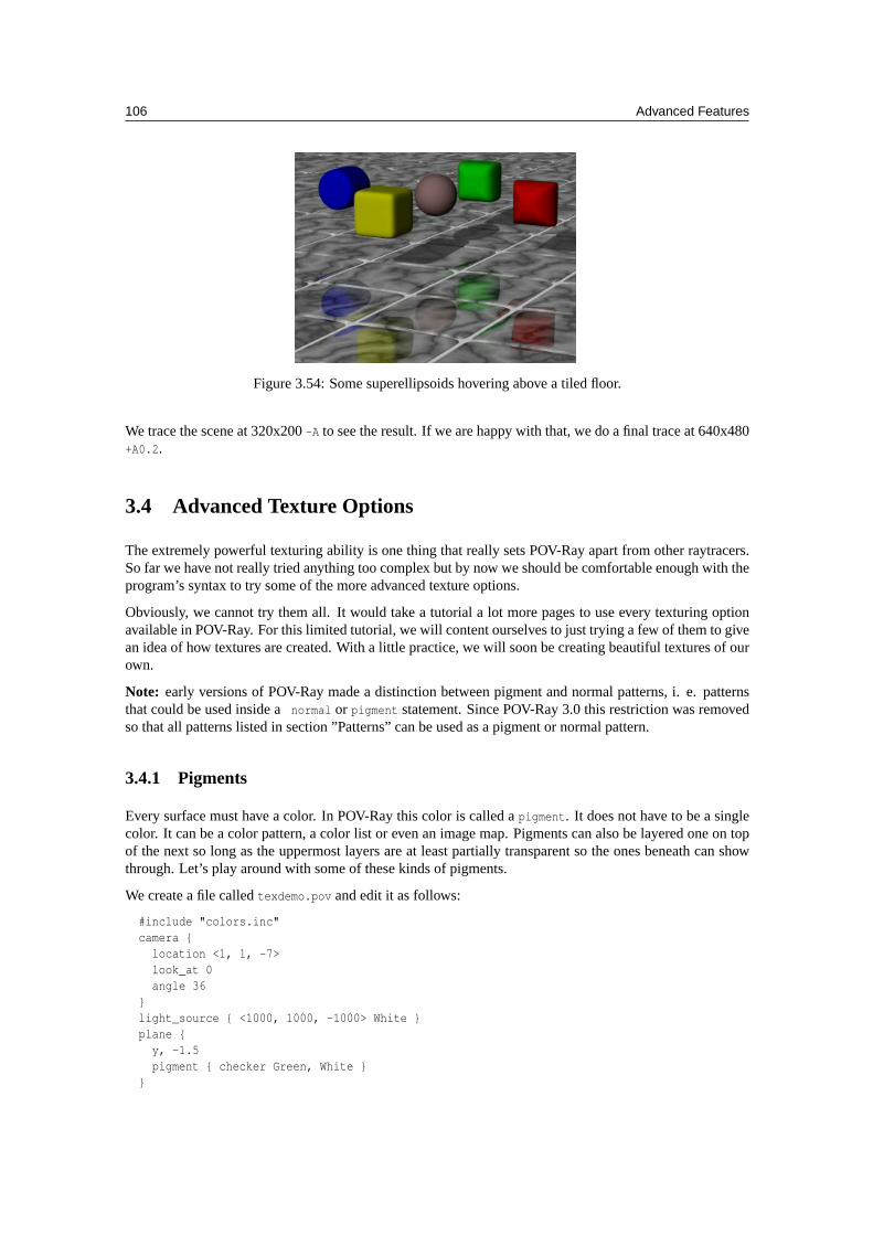
106 Advanced Features
Figure 3.54: Some superellipsoids hovering above a tiled floor.
We trace the scene at 320x200-A to see the result. If we are happy with that, we do a final trace at 640x480+A0.2.
3.4 Advanced Texture Options
The extremely powerful texturing ability is one thing that really sets POV-Ray apart from other raytracers.So far we have not really tried anything too complex but by now we should be comfortable enough with theprogram’s syntax to try some of the more advanced texture options.
Obviously, we cannot try them all. It would take a tutorial a lot more pages to use every texturing optionavailable in POV-Ray. For this limited tutorial, we will content ourselves to just trying a few of them to givean idea of how textures are created. With a little practice, we will soon be creating beautiful textures of ourown.
Note: early versions of POV-Ray made a distinction between pigment and normal patterns, i. e. patternsthat could be used inside anormal or pigment statement. Since POV-Ray 3.0 this restriction was removedso that all patterns listed in section ”Patterns” can be used as a pigment or normal pattern.
3.4.1 Pigments
Every surface must have a color. In POV-Ray this color is called apigment. It does not have to be a singlecolor. It can be a color pattern, a color list or even an image map. Pigments can also be layered one on topof the next so long as the uppermost layers are at least partially transparent so the ones beneath can showthrough. Let’s play around with some of these kinds of pigments.
We create a file calledtexdemo.pov and edit it as follows:
#include "colors.inc"camera {
location <1, 1, -7>look_at 0angle 36
}light_source { <1000, 1000, -1000> White }plane {
y, -1.5pigment { checker Green, White }
}
3.4 Advanced Texture Options 107
sphere {<0,0,0>, 1pigment { Red }
}
Giving this file a quick test render at 200x150-A we see that it is a simple red sphere against a green andwhite checkered plane. We will be using the sphere for our textures.
Using Color List Pigments
Before we begin we should note that we have already made one kind of pigment, the color list pigment. Inthe previous example we have used a checkered pattern on our plane. There are three other kinds of colorlist pigments,brick, hexagon and theobject pattern. Let’s quickly try each of these. First, we change theplane’s pigment as follows:
pigment { hexagon Green, White, Yellow }
Rendering this we see a three-color hexagonal pattern. Note that this pattern requires three colors. Now wechange the pigment to...
pigment { brick Gray75, Red rotate -90*x scale .25 }
Looking at the resulting image we see that the plane now has a brick pattern. We note that we had to rotatethe pattern to make it appear correctly on the flat plane. This pattern normally is meant to be used on verticalsurfaces. We also had to scale the pattern down a bit so we could see it more easily. We can play aroundwith these color list pigments, change the colors, etc. until we get a floor that we like.
Using Pigment and Patterns
Let’s begin texturing our sphere by using a pattern and a color map consisting of three colors. We replacethe pigment block with the following.
pigment {gradient xcolor_map {
[0.00 color Red][0.33 color Blue][0.66 color Yellow][1.00 color Red]
}}
Rendering this we see that thegradient pattern gives us an interesting pattern of vertical stripes. We changethe gradient direction to y. The stripes are horizontal now. We change the gradient direction to z. The stripesare now more like concentric rings. This is because the gradient direction is directly away from the camera.We change the direction back to x and add the following to the pigment block.
pigment {gradient xcolor_map {
[0.00 color Red][0.33 color Blue][0.66 color Yellow][1.00 color Red]
}rotate -45*z // <- add this line
}
108 Advanced Features
The vertical bars are now slanted at a 45 degree angle. All patterns can be rotated, scaled and translatedin this manner. Let’s now try some different types of patterns. One at a time, we substitute the followingkeywords forgradient x and render to see the result:bozo, marble, agate, granite, leopard, spotted andwood (if we like we can test all patterns listed in section ”Patterns”).
Rendering these we see that each results in a slightly different pattern. But to get really good results eachtype of pattern requires the use of some pattern modifiers.
Using Pattern Modifiers
Let’s take a look at some pattern modifiers. First, we change the pattern type to bozo. Then we add thefollowing change.
pigment {bozofrequency 3 // <- add this linecolor_map {
[0.00 color Red][0.33 color Blue][0.66 color Yellow][1.00 color Red]
}rotate -45*z
}
Thefrequency modifier determines the number of times the color map repeats itself per unit of size. Thischange makes thebozo pattern we saw earlier have many more bands in it. Now we change the pattern typeto marble. When we rendered this earlier, we saw a banded pattern similar togradient y that really did notlook much like marble at all. This is because marble really is a kind of gradient and it needs another patternmodifier to look like marble. This modifier is calledturbulence. We change the linefrequency 3 toturbulence 1 and render again. That’s better! Now let’s putfrequency 3 back in right after the turbulenceand take another look. Even more interesting!
But wait, it gets better! Turbulence itself has some modifiers of its own. We can adjust the turbulenceseveral ways. First, the float that follows theturbulence keyword can be any value with higher valuesgiving us more turbulence. Second, we can use the keywordsomega, lambda andoctaves to change theturbulence parameters.
Let’s try this now:
pigment {marbleturbulence 0.5lambda 1.5omega 0.8octaves 5frequency 3color_map {
[0.00 color Red][0.33 color Blue][0.66 color Yellow][1.00 color Red]
}rotate 45*z
}
Rendering this we see that the turbulence has changed and the pattern looks different. We play around withthe numerical values of turbulence, lambda, omega and octaves to see what they do.
3.4 Advanced Texture Options 109
Using Transparent Pigments and Layered Textures
Pigments are described by numerical values that give the rgb value of the color to be used (likecolor
rgb<1,0,0> giving us a red color). But this syntax will give us more than just the rgb values. We canspecify filtering transparency by changing it as follows:color rgbf<1,0,0,1>. The f stands forfilter,POV-Ray’s word for filtered transparency. A value of one means that the color is completely transparent,but still filters the light according to what the pigment is. In this case, the color will be a transparent red,like red cellophane.
There is another kind of transparency in POV-Ray. It is calledtransmittanceor non-filtering transparency(the keyword istransmit; see alsorgbt). It is different fromfilter in that it does not filter the lightaccording to the pigment color. It instead allows all the light to pass through unchanged. It can be specifiedlike this: rgbt <1,0,0,1>.
Let’s use some transparent pigments to create another kind of texture, the layered texture. Returning to ourprevious example, declare the following texture.
#declare LandArea = texture {pigment {
agateturbulence 1lambda 1.5omega .8octaves 8color_map {
[0.00 color rgb <.5, .25, .15>][0.33 color rgb <.1, .5, .4>][0.86 color rgb <.6, .3, .1>][1.00 color rgb <.5, .25, .15>]
}}
}
This texture will be the land area. Now let’s make the oceans by declaring the following.
#declare OceanArea = texture {pigment {
bozoturbulence .5lambda 2color_map {
[0.00, 0.33 color rgb <0, 0, 1>color rgb <0, 0, 1>]
[0.33, 0.66 color rgbf <1, 1, 1, 1>color rgbf <1, 1, 1, 1>]
[0.66, 1.00 color rgb <0, 0, 1>color rgb <0, 0, 1>]
}}
}
Note: how the ocean is the opaque blue area and the land is the clear area which will allow the underlyingtexture to show through.
Now, let’s declare one more texture to simulate an atmosphere with swirling clouds.
#declare CloudArea = texture {pigment {
agateturbulence 1
110 Advanced Features
lambda 2frequency 2color_map {
[0.0 color rgbf <1, 1, 1, 1>][0.5 color rgbf <1, 1, 1, .35>][1.0 color rgbf <1, 1, 1, 1>]
}}
}
Now apply all of these to our sphere.
sphere {<0,0,0>, 1texture { LandArea }texture { OceanArea }texture { CloudArea }
}
We render this and have a pretty good rendition of a little planetoid. But it could be better. We do notparticularly like the appearance of the clouds. There is a way they could be done that would be much morerealistic.
Using Pigment Maps
Pigments may be blended together in the same way as the colors in a color map using the same patternkeywords and apigment map. Let’s just give it a try.
We add the following declarations, making sure they appear before the other declarations in the file.
#declare Clouds1 = pigment {bozoturbulence 1color_map {
[0.0 color White filter 1][0.5 color White][1.0 color White filter 1]
}}
#declare Clouds2 = pigment {agateturbulence 1color_map {
[0.0 color White filter 1][0.5 color White][1.0 color White filter 1]}
}#declare Clouds3 = pigment {
marbleturbulence 1color_map {
[0.0 color White filter 1][0.5 color White][1.0 color White filter 1]
}}#declare Clouds4 = pigment {
3.4 Advanced Texture Options 111
graniteturbulence 1color_map {[0.0 color White filter 1][0.5 color White][1.0 color White filter 1]
}}
Now we use these declared pigments in our cloud layer on our planetoid. We replace the declared cloudlayer with.
#declare CloudArea = texture {pigment {
gradient ypigment_map {
[0.00 Clouds1][0.25 Clouds2][0.50 Clouds3][0.75 Clouds4][1.00 Clouds1]
}}
}
We render this and see a remarkable pattern that looks very much like weather patterns on the planet earth.They are separated into bands, simulating the different weather types found at different latitudes.
3.4.2 Normals
Objects in POV-Ray have very smooth surfaces. This is not very realistic so there are several ways todisturb the smoothness of an object by perturbing the surface normal. The surface normal is the vector thatis perpendicular to the angle of the surface. By changing this normal the surface can be made to appearbumpy, wrinkled or any of the many patterns available. Let’s try a couple of them.
Using Basic Normal Modifiers
We comment out the planetoid sphere for now and, at the bottom of the file, create a new sphere with asimple, single color texture.
sphere {<0,0,0>, 1pigment { Gray75 }normal { bumps 1 scale .2 }
}
Here we have added anormal block in addition to the pigment block (note that these do not have to beincluded in a texture block unless they need to be transformed together or need to be part of a layeredtexture). We render this to see what it looks like. Now, one at a time, we substitute for the keywordbumps
the following keywords:dents, wrinkles, ripples andwaves (we can also use any of the patterns listed in”Patterns”). We render each to see what they look like. We play around with the float value that follows thekeyword. We also experiment with the scale value.
For added interest, we change the plane texture to a single color with a normal as follows.
plane {y, -1.5
112 Advanced Features
pigment { color rgb <.65, .45, .35> }normal { dents .75 scale .25 }
}
Blending Normals
Normals can be layered similar to pigments but the results can be unexpected. Let’s try that now by editingthe sphere as follows.
sphere {<0,0,0>, 1pigment { Gray75 }
normal { radial frequency 10 }normal { gradient y scale .2 }
}
As we can see, the resulting pattern is neither a radial nor a gradient. It is instead the result of first calculatinga radial pattern and then calculating a gradient pattern. The results are simply additive. This can be difficultto control so POV-Ray gives the user other ways to blend normals.
One way is to use normal maps. A normal map works the same way as the pigment map we used earlier.Let’s change our sphere texture as follows.
sphere {<0,0,0>, 1pigment { Gray75 }normal {
gradient yfrequency 3turbulence .5normal_map {
[0.00 granite][0.25 spotted turbulence .35][0.50 marble turbulence .5][0.75 bozo turbulence .25][1.00 granite]
}}
}
Rendering this we see that the sphere now has a very irregular bumpy surface. The gradient pattern typeseparates the normals into bands but they are turbulated, giving the surface a chaotic appearance. But thisgives us an idea.
Suppose we use the same pattern for a normal map that we used to create the oceans on our planetoid andapplied it to the land areas. Does it follow that if we use the same pattern and modifiers on a sphere thesame size that the shape of the pattern would be the same? Would not that make the land areas bumpy whileleaving the oceans smooth? Let’s try it. First, let’s render the two spheres side-by-side so we can see if thepattern is indeed the same. We un-comment the planetoid sphere and make the following changes.
sphere {<0,0,0>, 1texture { LandArea }texture { OceanArea }//texture { CloudArea } // <-comment this outtranslate -x // <- add this transformation
}
Now we change the gray sphere as follows.
3.4 Advanced Texture Options 113
sphere {<0,0,0>, 1pigment { Gray75 }normal {
bozoturbulence .5lambda 2normal_map {
[0.4 dents .15 scale .01][0.6 agate turbulence 1][1.0 dents .15 scale .01]
}}translate x // <- add this transformation
}
We render this to see if the pattern is the same. We see that indeed it is. So let’s comment out the graysphere and add thenormal block it contains to the land area texture of our planetoid. We remove thetransformations so that the planetoid is centered in the scene again.
#declare LandArea = texture {pigment {
agateturbulence 1lambda 1.5omega .8octaves 8color_map {
[0.00 color rgb <.5, .25, .15>][0.33 color rgb <.1, .5, .4>][0.86 color rgb <.6, .3, .1>][1.00 color rgb <.5, .25, .15>]
}}normal {
bozoturbulence .5lambda 2normal_map {
[0.4 dents .15 scale .01][0.6 agate turbulence 1][1.0 dents .15 scale .01]
}}
}
Looking at the resulting image we see that indeed our idea works! The land areas are bumpy while theoceans are smooth. We add the cloud layer back in and our planetoid is complete.
There is much more that we did not cover here due to space constraints. On our own, we should take thetime to explore slope maps, average and bump maps.
3.4.3 Finishes
The final part of a POV-Ray texture is thefinish. It controls the properties of the surface of an object. It canmake it shiny and reflective, or dull and flat. It can also specify what happens to light that passes throughtransparent pigments, what happens to light that is scattered by less-than-perfectly-smooth surfaces and
114 Advanced Features
what happens to light that is reflected by surfaces with thin-film interference properties. There are twelvedifferent properties available in POV-Ray to specify the finish of a given object. These are controlled bythe following keywords:ambient, diffuse, brilliance, phong, specular, metallic, reflection, crand andiridescence. Let’s design a couple of textures that make use of these parameters.
Using Ambient
Since objects in POV-Ray are illuminated by light sources, the portions of those objects that are in shadowwould be completely black were it not for the first two finish properties,ambient anddiffuse. Ambientis used to simulate the light that is scattered around the scene that does not come directly from a lightsource. Diffuse determines how much of the light that is seen comes directly from a light source. These twokeywords work together to control the simulation of ambient light. Let’s use our gray sphere to demonstratethis. Let’s also change our plane back to its original green and white checkered pattern.
plane {y, -1.5pigment {checker Green, White}
}sphere {
<0,0,0>, 1pigment { Gray75 }finish {
ambient .2diffuse .6
}}
In the above example, the default values for ambient and diffuse are used. We render this to see what theeffect is and then make the following change to the finish.
ambient 0diffuse 0
The sphere is black because we have specified that none of the light coming from any light source will bereflected by the sphere. Let’s changediffuse back to the default of 0.6.
Now we see the gray surface color where the light from the light source falls directly on the sphere but theshaded side is still absolutely black. Now let’s changediffuse to 0.3 andambient to 0.3.
The sphere now looks almost flat. This is because we have specified a fairly high degree of ambient lightand only a low amount of the light coming from the light source is diffusely reflected towards the camera.The default values ofambient anddiffuse are pretty good averages and a good starting point. In mostcases, an ambient value of 0.1 ... 0.2 is sufficient and a diffuse value of 0.5 ... 0.7 will usually do the job.There are a couple of exceptions. If we have a completely transparent surface with high refractive and/orreflective values, low values of both ambient and diffuse may be best. Here is an example:
sphere {<0,0,0>, 1pigment { White filter 1 }finish {
ambient 0diffuse 0reflection .25specular 1roughness .001
}interior { ior 1.33 }
}
3.4 Advanced Texture Options 115
This is glass, obviously. Glass is a material that takes nearly all of its appearance from its surroundings.Very little of the surface is seen because it transmits or reflects practically all of the light that shines on it.Seeglass.inc for some other examples.
If we ever need an object to be completely illuminated independently of the lighting situation in a givenscene we can do this artificially by specifying anambient value of 1 and adiffuse value of 0. This willeliminate all shading and simply give the object its fullest and brightest color value at all points. This isgood for simulating objects that emit light like light bulbs and for skies in scenes where the sky may not beadequately lit by any other means.
Let’s try this with our sphere now.
sphere {<0,0,0>, 1pigment { White }finish {
ambient 1diffuse 0
}}
Rendering this we get a blinding white sphere with no visible highlights or shaded parts. It would make apretty good street light.
Using Surface Highlights
In the glass example above, we noticed that there were bright littlehotspotson the surface. This gave thesphere a hard, shiny appearance. POV-Ray gives us two ways to specify surface specular highlights. Thefirst is calledPhong highlighting.Usually, Phong highlights are described using two keywords:phong andphong size. The float that followsphong determines the brightness of the highlight while the float followingphong size determines its size. Let’s try this.
sphere {<0,0,0>, 1pigment { Gray50 }finish {
ambient .2diffuse .6phong .75phong_size 25
}}
Rendering this we see a fairly broad, soft highlight that gives the sphere a kind of plastic appearance.Now let’s change phong size to 150. This makes a much smaller highlight which gives the sphere theappearance of being much harder and shinier.
There is another kind of highlight that is calculated by a different means calledspecular highlighting. It isspecified using the keywordspecular and operates in conjunction with another keyword calledroughness.These two keywords work together in much the same way asphong andphong size to create highlights thatalter the apparent shininess of the surface. Let’s try using specular in our sphere.
sphere {<0,0,0>, 1pigment { Gray50 }finish {
ambient .2diffuse .6
116 Advanced Features
specular .75roughness .1
}}
Looking at the result we see a broad, soft highlight similar to what we had when we usedphong size of25. Changeroughness to .001 and render again. Now we see a small, tight highlight similar to what wehad when we usedphong size of 150. Generally speaking, specular is slightly more accurate and thereforeslightly more realistic than phong but you should try both methods when designing a texture. There areeven times when both phong and specular may be used on a finish.
Using Reflection, Metallic and Metallic
There is another surface parameter that goes hand in hand with highlights,reflection. Surfaces that arevery shiny usually have a degree of reflection to them. Let’s take a look at an example.
sphere {<0,0,0>, 1pigment { Gray50 }finish {
ambient .2diffuse .6specular .75roughness .001reflection {
.5}
}}
We see that our sphere now reflects the green and white checkered plane and the black background but thegray color of the sphere seems out of place. This is another time when a lower diffuse value is needed.Generally, the higherreflection is the lowerdiffuse should be. We lower the diffuse value to 0.3 and theambient value to 0.1 and render again. That is much better. Let’s make our sphere as shiny as a polishedgold ball bearing.
sphere {<0,0,0>, 1pigment { BrightGold }finish {
ambient .1diffuse .1specular 1roughness .001reflection {
.75}
}}
That is close but there is something wrong, the colour of the reflection and the highlight. To make thesurface appear more like metal the keywordmetallic is used. We add it now to see the difference.
sphere {<0,0,0>, 1pigment { BrightGold }finish {
ambient .1
3.4 Advanced Texture Options 117
diffuse .1specular 1roughness .001reflection {
.75metallic
}}
}
The reflection has now more of the gold color than the color of its environment. Last detail, the highlight.We add another metallic statement, now to the finish and not inside the reflection block.
sphere {<0,0,0>, 1pigment { BrightGold }finish {
ambient .1diffuse .1specular 1roughness .001metallicreflection {
.75metallic
}}
}
We see that the highlight has taken on the color of the surface rather than the light source. This gives thesurface a more metallic appearance.
Using Iridescence
Iridescenceis what we see on the surface of an oil slick when the sun shines on it. The rainbow effect iscreated by something calledthin-film interference(read section ”Iridescence” for details). For now let’sjust try using it. Iridescence is specified by theirid statement and three values: amount,thickness andturbulence. The amount is the contribution to the overall surface color. Usually 0.1 to 0.5 is sufficienthere. The thickness affects the ”busyness” of the effect. Keep this between 0.25 and 1 for best results. Theturbulence is a little different from pigment or normal turbulence. We cannot setoctaves, lambda or omegabut we can specify an amount which will affect the thickness in a slightly different way from the thicknessvalue. Values between 0.25 and 1 work best here too. Finally, iridescence will respond to the surface normalsince it depends on the angle of incidence of the light rays striking the surface. With all of this in mind,let’s add some iridescence to our glass sphere.
sphere {<0,0,0>, 1pigment { White filter 1 }finish {
ambient .1diffuse .1reflection .2specular 1roughness .001irid {
0.35thickness .5
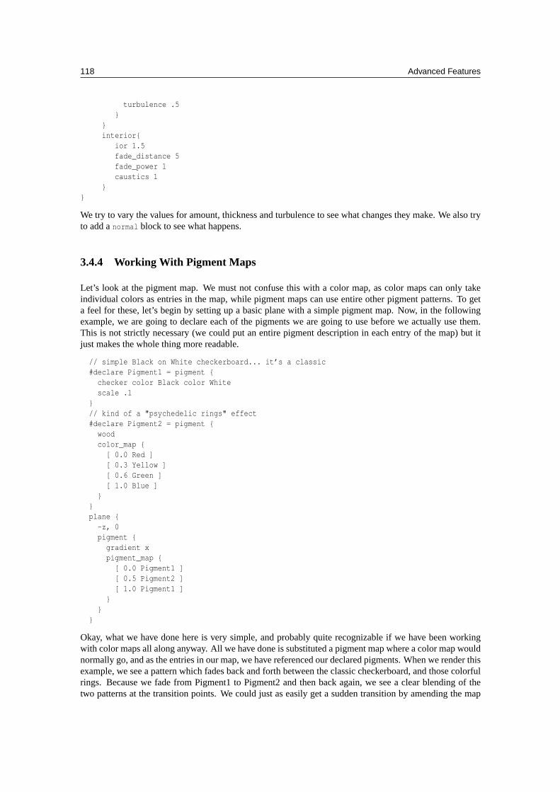
118 Advanced Features
turbulence .5}
}interior{
ior 1.5fade_distance 5fade_power 1caustics 1
}}
We try to vary the values for amount, thickness and turbulence to see what changes they make. We also tryto add anormal block to see what happens.
3.4.4 Working With Pigment Maps
Let’s look at the pigment map. We must not confuse this with a color map, as color maps can only takeindividual colors as entries in the map, while pigment maps can use entire other pigment patterns. To geta feel for these, let’s begin by setting up a basic plane with a simple pigment map. Now, in the followingexample, we are going to declare each of the pigments we are going to use before we actually use them.This is not strictly necessary (we could put an entire pigment description in each entry of the map) but itjust makes the whole thing more readable.
// simple Black on White checkerboard... it’s a classic#declare Pigment1 = pigment {
checker color Black color Whitescale .1
}// kind of a "psychedelic rings" effect#declare Pigment2 = pigment {
woodcolor_map {
[ 0.0 Red ][ 0.3 Yellow ][ 0.6 Green ][ 1.0 Blue ]
}}plane {
-z, 0pigment {
gradient xpigment_map {
[ 0.0 Pigment1 ][ 0.5 Pigment2 ][ 1.0 Pigment1 ]
}}
}
Okay, what we have done here is very simple, and probably quite recognizable if we have been workingwith color maps all along anyway. All we have done is substituted a pigment map where a color map wouldnormally go, and as the entries in our map, we have referenced our declared pigments. When we render thisexample, we see a pattern which fades back and forth between the classic checkerboard, and those colorfulrings. Because we fade from Pigment1 to Pigment2 and then back again, we see a clear blending of thetwo patterns at the transition points. We could just as easily get a sudden transition by amending the map
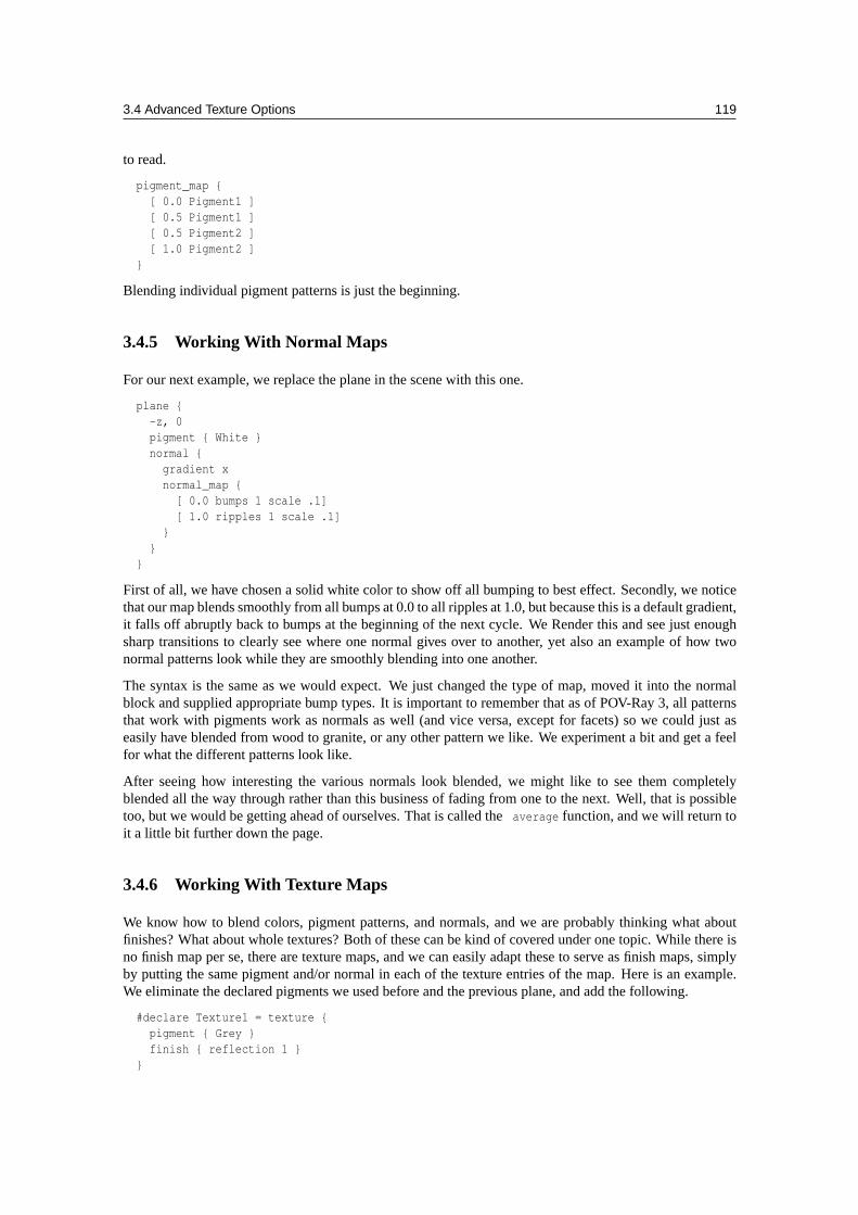
3.4 Advanced Texture Options 119
to read.
pigment_map {[ 0.0 Pigment1 ][ 0.5 Pigment1 ][ 0.5 Pigment2 ][ 1.0 Pigment2 ]
}
Blending individual pigment patterns is just the beginning.
3.4.5 Working With Normal Maps
For our next example, we replace the plane in the scene with this one.
plane {-z, 0pigment { White }normal {
gradient xnormal_map {
[ 0.0 bumps 1 scale .1][ 1.0 ripples 1 scale .1]
}}
}
First of all, we have chosen a solid white color to show off all bumping to best effect. Secondly, we noticethat our map blends smoothly from all bumps at 0.0 to all ripples at 1.0, but because this is a default gradient,it falls off abruptly back to bumps at the beginning of the next cycle. We Render this and see just enoughsharp transitions to clearly see where one normal gives over to another, yet also an example of how twonormal patterns look while they are smoothly blending into one another.
The syntax is the same as we would expect. We just changed the type of map, moved it into the normalblock and supplied appropriate bump types. It is important to remember that as of POV-Ray 3, all patternsthat work with pigments work as normals as well (and vice versa, except for facets) so we could just aseasily have blended from wood to granite, or any other pattern we like. We experiment a bit and get a feelfor what the different patterns look like.
After seeing how interesting the various normals look blended, we might like to see them completelyblended all the way through rather than this business of fading from one to the next. Well, that is possibletoo, but we would be getting ahead of ourselves. That is called theaverage function, and we will return toit a little bit further down the page.
3.4.6 Working With Texture Maps
We know how to blend colors, pigment patterns, and normals, and we are probably thinking what aboutfinishes? What about whole textures? Both of these can be kind of covered under one topic. While there isno finish map per se, there are texture maps, and we can easily adapt these to serve as finish maps, simplyby putting the same pigment and/or normal in each of the texture entries of the map. Here is an example.We eliminate the declared pigments we used before and the previous plane, and add the following.
#declare Texture1 = texture {pigment { Grey }finish { reflection 1 }
}
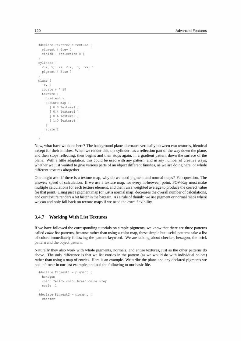
120 Advanced Features
#declare Texture2 = texture {pigment { Grey }finish { reflection 0 }
}cylinder {
<-2, 5, -2>, <-2, -5, -2>, 1pigment { Blue }
}plane {
-z, 0rotate y * 30texture {
gradient ytexture_map {
[ 0.0 Texture1 ][ 0.4 Texture1 ][ 0.6 Texture2 ][ 1.0 Texture2 ]
}scale 2
}}
Now, what have we done here? The background plane alternates vertically between two textures, identicalexcept for their finishes. When we render this, the cylinder has a reflection part of the way down the plane,and then stops reflecting, then begins and then stops again, in a gradient pattern down the surface of theplane. With a little adaptation, this could be used with any pattern, and in any number of creative ways,whether we just wanted to give various parts of an object different finishes, as we are doing here, or wholedifferent textures altogether.
One might ask: if there is a texture map, why do we need pigment and normal maps? Fair question. Theanswer: speed of calculation. If we use a texture map, for every in-between point, POV-Ray must makemultiple calculations for each texture element, and then run a weighted average to produce the correct valuefor that point. Using just a pigment map (or just a normal map) decreases the overall number of calculations,and our texture renders a bit faster in the bargain. As a rule of thumb: we use pigment or normal maps wherewe can and only fall back on texture maps if we need the extra flexibility.
3.4.7 Working With List Textures
If we have followed the corresponding tutorials on simple pigments, we know that there are three patternscalledcolor list patterns, because rather than using a color map, these simple but useful patterns take a listof colors immediately following the pattern keyword. We are talking about checker, hexagon, the brickpattern and the object pattern.
Naturally they also work with whole pigments, normals, and entire textures, just as the other patterns doabove. The only difference is that we list entries in the pattern (as we would do with individual colors)rather than using a map of entries. Here is an example. We strike the plane and any declared pigments wehad left over in our last example, and add the following to our basic file.
#declare Pigment1 = pigment {hexagoncolor Yellow color Green color Greyscale .1
}#declare Pigment2 = pigment {
checker
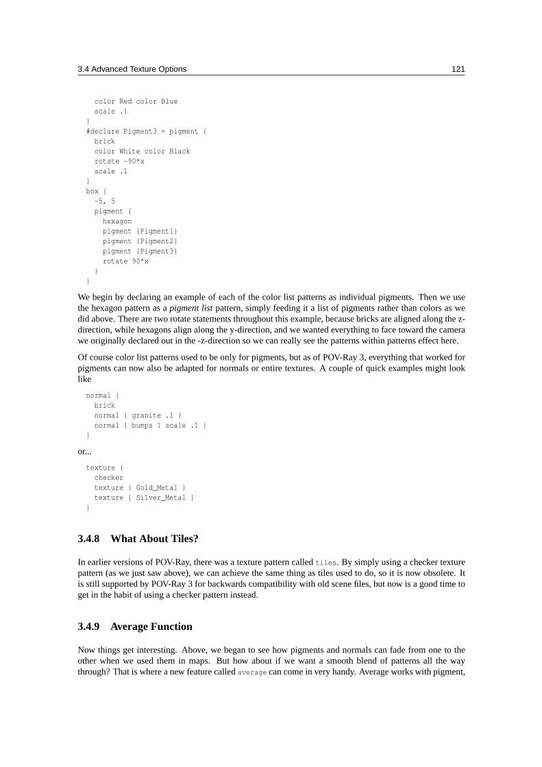
3.4 Advanced Texture Options 121
color Red color Bluescale .1
}#declare Pigment3 = pigment {
brickcolor White color Blackrotate -90*xscale .1
}box {
-5, 5pigment {
hexagonpigment {Pigment1}pigment {Pigment2}pigment {Pigment3}rotate 90*x
}}
We begin by declaring an example of each of the color list patterns as individual pigments. Then we usethe hexagon pattern as apigment listpattern, simply feeding it a list of pigments rather than colors as wedid above. There are two rotate statements throughout this example, because bricks are aligned along the z-direction, while hexagons align along the y-direction, and we wanted everything to face toward the camerawe originally declared out in the -z-direction so we can really see the patterns within patterns effect here.
Of course color list patterns used to be only for pigments, but as of POV-Ray 3, everything that worked forpigments can now also be adapted for normals or entire textures. A couple of quick examples might looklike
normal {bricknormal { granite .1 }normal { bumps 1 scale .1 }
}
or...
texture {checkertexture { Gold_Metal }texture { Silver_Metal }
}
3.4.8 What About Tiles?
In earlier versions of POV-Ray, there was a texture pattern calledtiles. By simply using a checker texturepattern (as we just saw above), we can achieve the same thing as tiles used to do, so it is now obsolete. Itis still supported by POV-Ray 3 for backwards compatibility with old scene files, but now is a good time toget in the habit of using a checker pattern instead.
3.4.9 Average Function
Now things get interesting. Above, we began to see how pigments and normals can fade from one to theother when we used them in maps. But how about if we want a smooth blend of patterns all the waythrough? That is where a new feature calledaverage can come in very handy. Average works with pigment,
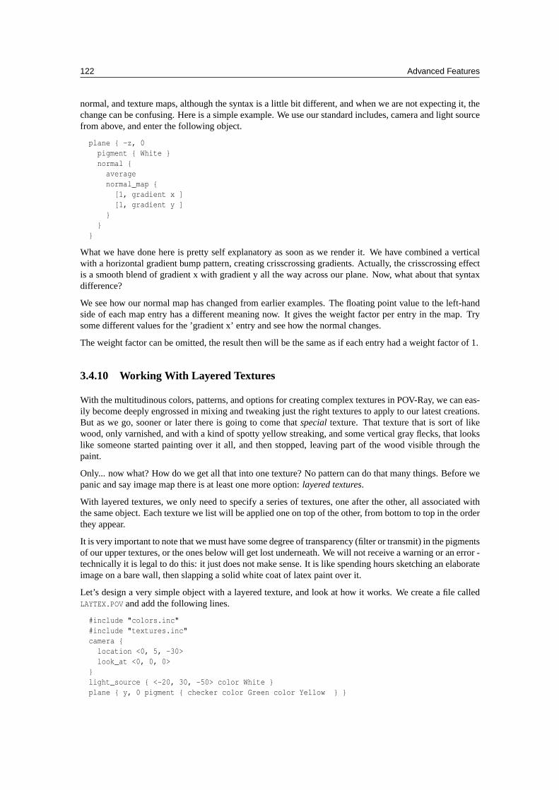
122 Advanced Features
normal, and texture maps, although the syntax is a little bit different, and when we are not expecting it, thechange can be confusing. Here is a simple example. We use our standard includes, camera and light sourcefrom above, and enter the following object.
plane { -z, 0pigment { White }normal {
averagenormal_map {
[1, gradient x ][1, gradient y ]
}}
}
What we have done here is pretty self explanatory as soon as we render it. We have combined a verticalwith a horizontal gradient bump pattern, creating crisscrossing gradients. Actually, the crisscrossing effectis a smooth blend of gradient x with gradient y all the way across our plane. Now, what about that syntaxdifference?
We see how our normal map has changed from earlier examples. The floating point value to the left-handside of each map entry has a different meaning now. It gives the weight factor per entry in the map. Trysome different values for the ’gradient x’ entry and see how the normal changes.
The weight factor can be omitted, the result then will be the same as if each entry had a weight factor of 1.
3.4.10 Working With Layered Textures
With the multitudinous colors, patterns, and options for creating complex textures in POV-Ray, we can eas-ily become deeply engrossed in mixing and tweaking just the right textures to apply to our latest creations.But as we go, sooner or later there is going to come thatspecialtexture. That texture that is sort of likewood, only varnished, and with a kind of spotty yellow streaking, and some vertical gray flecks, that lookslike someone started painting over it all, and then stopped, leaving part of the wood visible through thepaint.
Only... now what? How do we get all that into one texture? No pattern can do that many things. Before wepanic and say image map there is at least one more option:layered textures.
With layered textures, we only need to specify a series of textures, one after the other, all associated withthe same object. Each texture we list will be applied one on top of the other, from bottom to top in the orderthey appear.
It is very important to note that we must have some degree of transparency (filter or transmit) in the pigmentsof our upper textures, or the ones below will get lost underneath. We will not receive a warning or an error -technically it is legal to do this: it just does not make sense. It is like spending hours sketching an elaborateimage on a bare wall, then slapping a solid white coat of latex paint over it.
Let’s design a very simple object with a layered texture, and look at how it works. We create a file calledLAYTEX.POV and add the following lines.
#include "colors.inc"#include "textures.inc"camera {
location <0, 5, -30>look_at <0, 0, 0>
}light_source { <-20, 30, -50> color White }plane { y, 0 pigment { checker color Green color Yellow } }
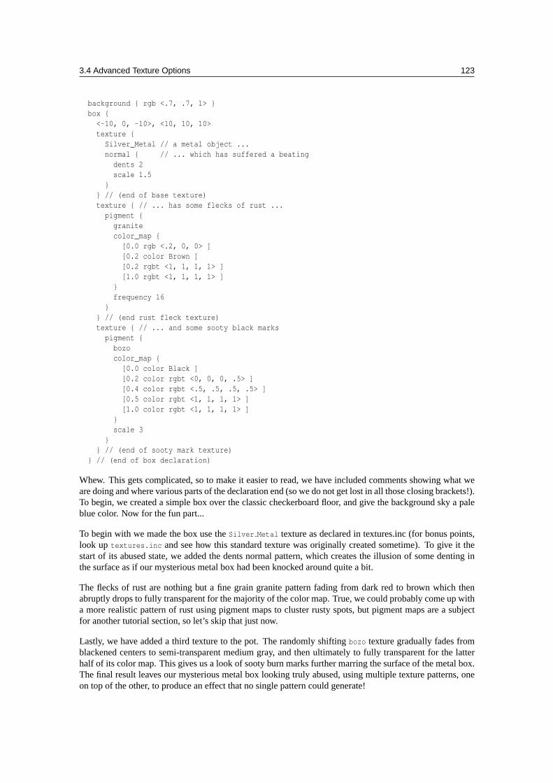
3.4 Advanced Texture Options 123
background { rgb <.7, .7, 1> }box {
<-10, 0, -10>, <10, 10, 10>texture {
Silver_Metal // a metal object ...normal { // ... which has suffered a beating
dents 2scale 1.5
}} // (end of base texture)texture { // ... has some flecks of rust ...
pigment {granitecolor_map {
[0.0 rgb <.2, 0, 0> ][0.2 color Brown ][0.2 rgbt <1, 1, 1, 1> ][1.0 rgbt <1, 1, 1, 1> ]
}frequency 16
}} // (end rust fleck texture)texture { // ... and some sooty black marks
pigment {bozocolor_map {
[0.0 color Black ][0.2 color rgbt <0, 0, 0, .5> ][0.4 color rgbt <.5, .5, .5, .5> ][0.5 color rgbt <1, 1, 1, 1> ][1.0 color rgbt <1, 1, 1, 1> ]
}scale 3
}} // (end of sooty mark texture)
} // (end of box declaration)
Whew. This gets complicated, so to make it easier to read, we have included comments showing what weare doing and where various parts of the declaration end (so we do not get lost in all those closing brackets!).To begin, we created a simple box over the classic checkerboard floor, and give the background sky a paleblue color. Now for the fun part...
To begin with we made the box use theSilver Metal texture as declared in textures.inc (for bonus points,look up textures.inc and see how this standard texture was originally created sometime). To give it thestart of its abused state, we added the dents normal pattern, which creates the illusion of some denting inthe surface as if our mysterious metal box had been knocked around quite a bit.
The flecks of rust are nothing but a fine grain granite pattern fading from dark red to brown which thenabruptly drops to fully transparent for the majority of the color map. True, we could probably come up witha more realistic pattern of rust using pigment maps to cluster rusty spots, but pigment maps are a subjectfor another tutorial section, so let’s skip that just now.
Lastly, we have added a third texture to the pot. The randomly shiftingbozo texture gradually fades fromblackened centers to semi-transparent medium gray, and then ultimately to fully transparent for the latterhalf of its color map. This gives us a look of sooty burn marks further marring the surface of the metal box.The final result leaves our mysterious metal box looking truly abused, using multiple texture patterns, oneon top of the other, to produce an effect that no single pattern could generate!
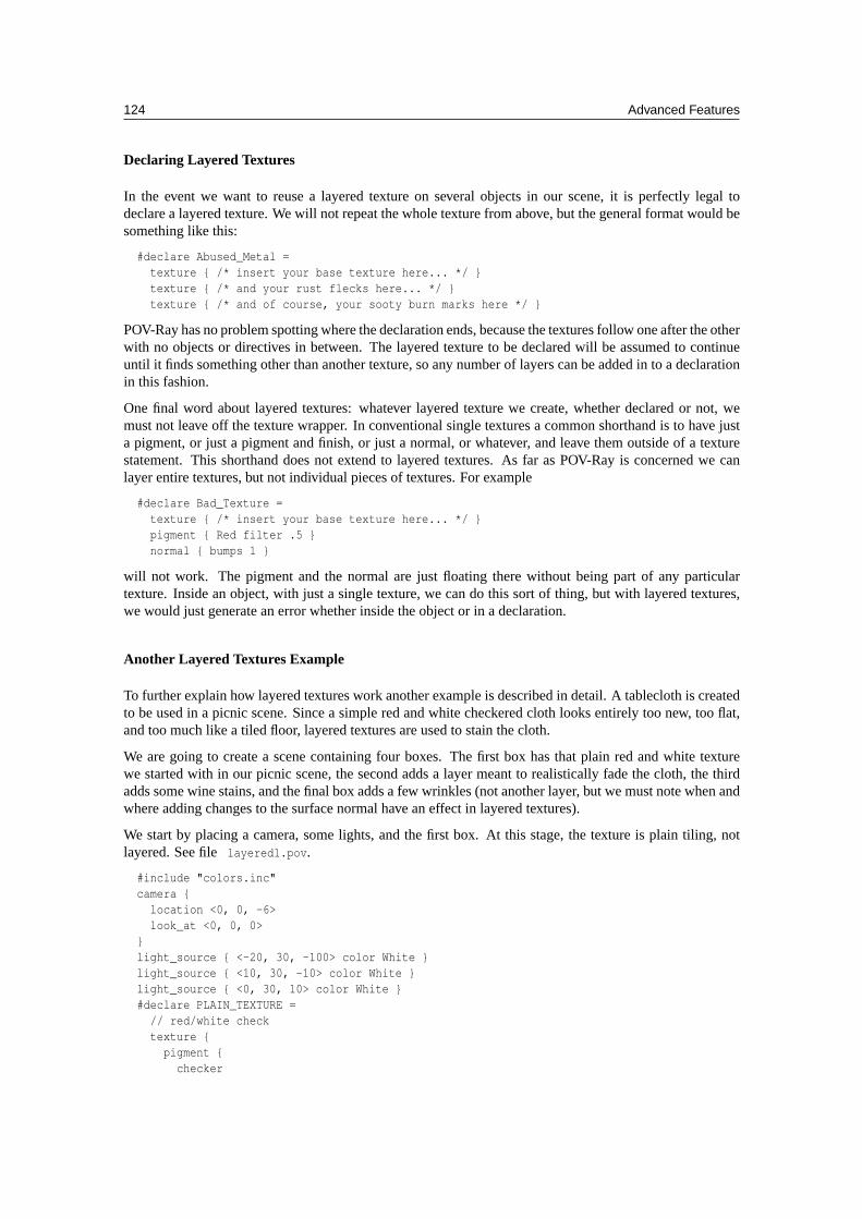
124 Advanced Features
Declaring Layered Textures
In the event we want to reuse a layered texture on several objects in our scene, it is perfectly legal todeclare a layered texture. We will not repeat the whole texture from above, but the general format would besomething like this:
#declare Abused_Metal =texture { /* insert your base texture here... */ }texture { /* and your rust flecks here... */ }texture { /* and of course, your sooty burn marks here */ }
POV-Ray has no problem spotting where the declaration ends, because the textures follow one after the otherwith no objects or directives in between. The layered texture to be declared will be assumed to continueuntil it finds something other than another texture, so any number of layers can be added in to a declarationin this fashion.
One final word about layered textures: whatever layered texture we create, whether declared or not, wemust not leave off the texture wrapper. In conventional single textures a common shorthand is to have justa pigment, or just a pigment and finish, or just a normal, or whatever, and leave them outside of a texturestatement. This shorthand does not extend to layered textures. As far as POV-Ray is concerned we canlayer entire textures, but not individual pieces of textures. For example
#declare Bad_Texture =texture { /* insert your base texture here... */ }pigment { Red filter .5 }normal { bumps 1 }
will not work. The pigment and the normal are just floating there without being part of any particulartexture. Inside an object, with just a single texture, we can do this sort of thing, but with layered textures,we would just generate an error whether inside the object or in a declaration.
Another Layered Textures Example
To further explain how layered textures work another example is described in detail. A tablecloth is createdto be used in a picnic scene. Since a simple red and white checkered cloth looks entirely too new, too flat,and too much like a tiled floor, layered textures are used to stain the cloth.
We are going to create a scene containing four boxes. The first box has that plain red and white texturewe started with in our picnic scene, the second adds a layer meant to realistically fade the cloth, the thirdadds some wine stains, and the final box adds a few wrinkles (not another layer, but we must note when andwhere adding changes to the surface normal have an effect in layered textures).
We start by placing a camera, some lights, and the first box. At this stage, the texture is plain tiling, notlayered. See filelayered1.pov.
#include "colors.inc"camera {
location <0, 0, -6>look_at <0, 0, 0>
}light_source { <-20, 30, -100> color White }light_source { <10, 30, -10> color White }light_source { <0, 30, 10> color White }#declare PLAIN_TEXTURE =
// red/white checktexture {
pigment {checker
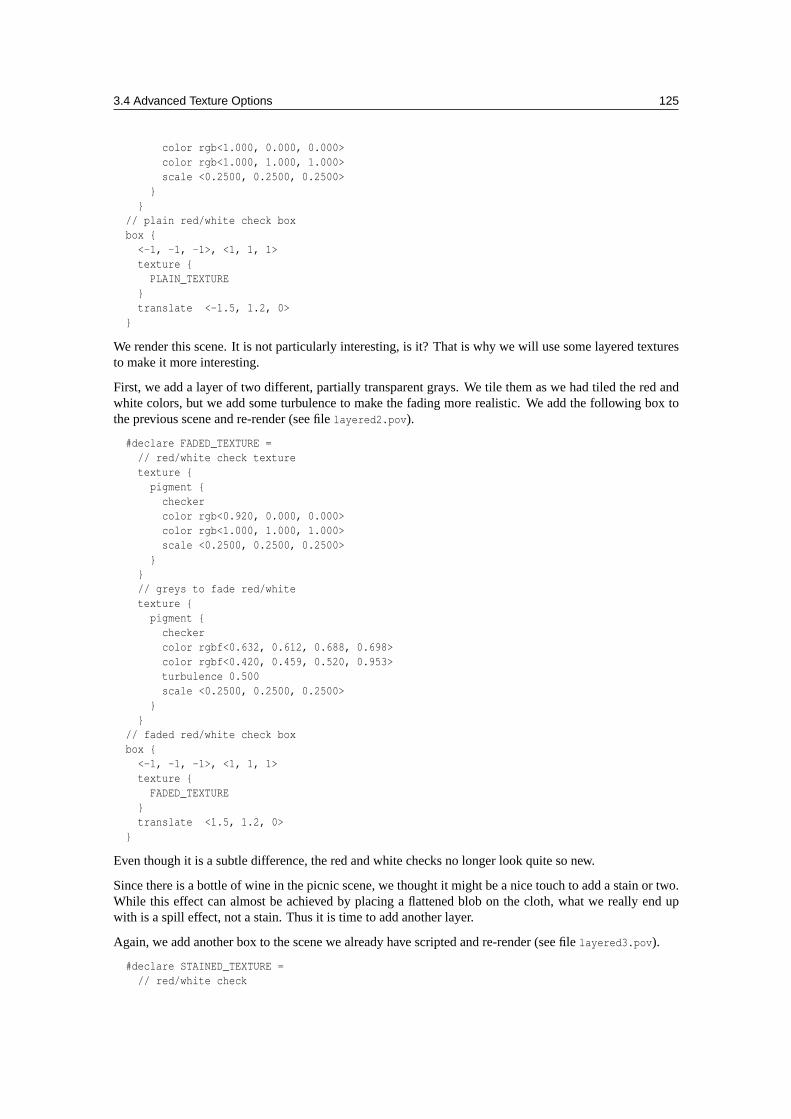
3.4 Advanced Texture Options 125
color rgb<1.000, 0.000, 0.000>color rgb<1.000, 1.000, 1.000>scale <0.2500, 0.2500, 0.2500>
}}
// plain red/white check boxbox {
<-1, -1, -1>, <1, 1, 1>texture {
PLAIN_TEXTURE}translate <-1.5, 1.2, 0>
}
We render this scene. It is not particularly interesting, is it? That is why we will use some layered texturesto make it more interesting.
First, we add a layer of two different, partially transparent grays. We tile them as we had tiled the red andwhite colors, but we add some turbulence to make the fading more realistic. We add the following box tothe previous scene and re-render (see filelayered2.pov).
#declare FADED_TEXTURE =// red/white check texturetexture {
pigment {checkercolor rgb<0.920, 0.000, 0.000>color rgb<1.000, 1.000, 1.000>scale <0.2500, 0.2500, 0.2500>
}}// greys to fade red/whitetexture {
pigment {checkercolor rgbf<0.632, 0.612, 0.688, 0.698>color rgbf<0.420, 0.459, 0.520, 0.953>turbulence 0.500scale <0.2500, 0.2500, 0.2500>
}}
// faded red/white check boxbox {
<-1, -1, -1>, <1, 1, 1>texture {
FADED_TEXTURE}translate <1.5, 1.2, 0>
}
Even though it is a subtle difference, the red and white checks no longer look quite so new.
Since there is a bottle of wine in the picnic scene, we thought it might be a nice touch to add a stain or two.While this effect can almost be achieved by placing a flattened blob on the cloth, what we really end upwith is a spill effect, not a stain. Thus it is time to add another layer.
Again, we add another box to the scene we already have scripted and re-render (see filelayered3.pov).
#declare STAINED_TEXTURE =// red/white check
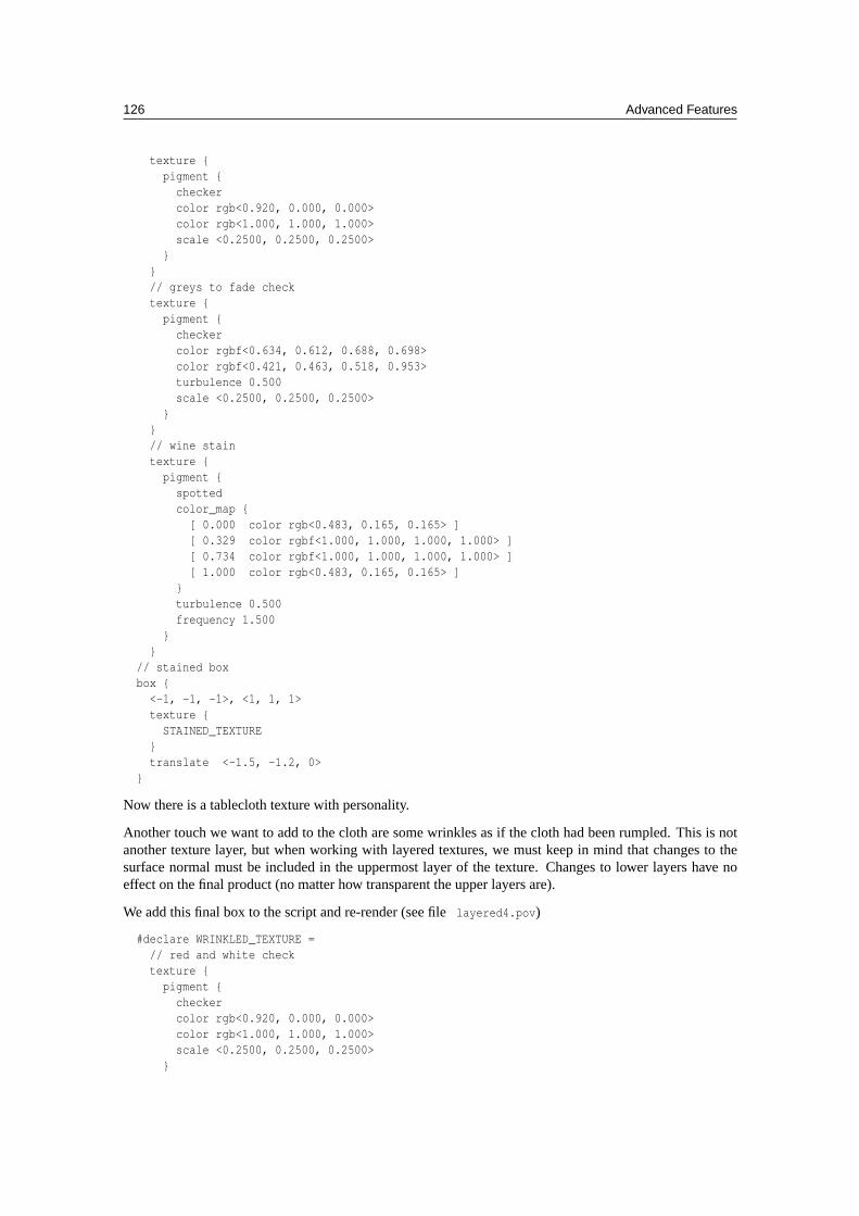
126 Advanced Features
texture {pigment {
checkercolor rgb<0.920, 0.000, 0.000>color rgb<1.000, 1.000, 1.000>scale <0.2500, 0.2500, 0.2500>
}}// greys to fade checktexture {
pigment {checkercolor rgbf<0.634, 0.612, 0.688, 0.698>color rgbf<0.421, 0.463, 0.518, 0.953>turbulence 0.500scale <0.2500, 0.2500, 0.2500>
}}// wine staintexture {
pigment {spottedcolor_map {
[ 0.000 color rgb<0.483, 0.165, 0.165> ][ 0.329 color rgbf<1.000, 1.000, 1.000, 1.000> ][ 0.734 color rgbf<1.000, 1.000, 1.000, 1.000> ][ 1.000 color rgb<0.483, 0.165, 0.165> ]
}turbulence 0.500frequency 1.500
}}
// stained boxbox {
<-1, -1, -1>, <1, 1, 1>texture {
STAINED_TEXTURE}translate <-1.5, -1.2, 0>
}
Now there is a tablecloth texture with personality.
Another touch we want to add to the cloth are some wrinkles as if the cloth had been rumpled. This is notanother texture layer, but when working with layered textures, we must keep in mind that changes to thesurface normal must be included in the uppermost layer of the texture. Changes to lower layers have noeffect on the final product (no matter how transparent the upper layers are).
We add this final box to the script and re-render (see filelayered4.pov)
#declare WRINKLED_TEXTURE =// red and white checktexture {
pigment {checkercolor rgb<0.920, 0.000, 0.000>color rgb<1.000, 1.000, 1.000>scale <0.2500, 0.2500, 0.2500>
}
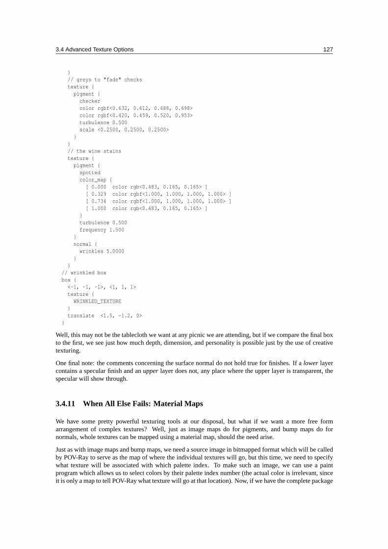
3.4 Advanced Texture Options 127
}// greys to "fade" checkstexture {pigment {
checkercolor rgbf<0.632, 0.612, 0.688, 0.698>color rgbf<0.420, 0.459, 0.520, 0.953>turbulence 0.500scale <0.2500, 0.2500, 0.2500>
}}// the wine stainstexture {
pigment {spottedcolor_map {
[ 0.000 color rgb<0.483, 0.165, 0.165> ][ 0.329 color rgbf<1.000, 1.000, 1.000, 1.000> ][ 0.734 color rgbf<1.000, 1.000, 1.000, 1.000> ][ 1.000 color rgb<0.483, 0.165, 0.165> ]
}turbulence 0.500frequency 1.500
}normal {
wrinkles 5.0000}
}// wrinkled boxbox {
<-1, -1, -1>, <1, 1, 1>texture {
WRINKLED_TEXTURE}translate <1.5, -1.2, 0>
}
Well, this may not be the tablecloth we want at any picnic we are attending, but if we compare the final boxto the first, we see just how much depth, dimension, and personality is possible just by the use of creativetexturing.
One final note: the comments concerning the surface normal do not hold true for finishes. If alower layercontains a specular finish and anupper layer does not, any place where the upper layer is transparent, thespecular will show through.
3.4.11 When All Else Fails: Material Maps
We have some pretty powerful texturing tools at our disposal, but what if we want a more free formarrangement of complex textures? Well, just as image maps do for pigments, and bump maps do fornormals, whole textures can be mapped using a material map, should the need arise.
Just as with image maps and bump maps, we need a source image in bitmapped format which will be calledby POV-Ray to serve as the map of where the individual textures will go, but this time, we need to specifywhat texture will be associated with which palette index. To make such an image, we can use a paintprogram which allows us to select colors by their palette index number (the actual color is irrelevant, sinceit is only a map to tell POV-Ray what texture will go at that location). Now, if we have the complete package
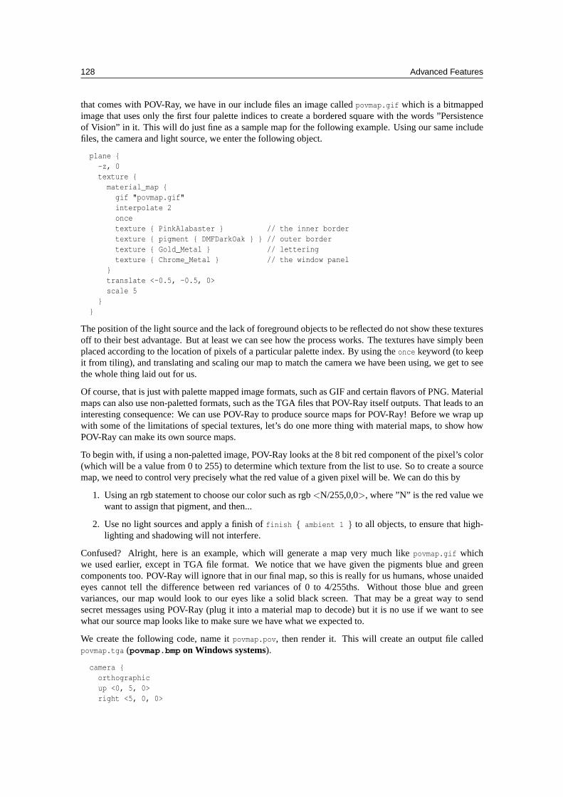
128 Advanced Features
that comes with POV-Ray, we have in our include files an image calledpovmap.gif which is a bitmappedimage that uses only the first four palette indices to create a bordered square with the words ”Persistenceof Vision” in it. This will do just fine as a sample map for the following example. Using our same includefiles, the camera and light source, we enter the following object.
plane {-z, 0texture {
material_map {gif "povmap.gif"interpolate 2oncetexture { PinkAlabaster } // the inner bordertexture { pigment { DMFDarkOak } } // outer bordertexture { Gold_Metal } // letteringtexture { Chrome_Metal } // the window panel
}translate <-0.5, -0.5, 0>scale 5
}}
The position of the light source and the lack of foreground objects to be reflected do not show these texturesoff to their best advantage. But at least we can see how the process works. The textures have simply beenplaced according to the location of pixels of a particular palette index. By using theonce keyword (to keepit from tiling), and translating and scaling our map to match the camera we have been using, we get to seethe whole thing laid out for us.
Of course, that is just with palette mapped image formats, such as GIF and certain flavors of PNG. Materialmaps can also use non-paletted formats, such as the TGA files that POV-Ray itself outputs. That leads to aninteresting consequence: We can use POV-Ray to produce source maps for POV-Ray! Before we wrap upwith some of the limitations of special textures, let’s do one more thing with material maps, to show howPOV-Ray can make its own source maps.
To begin with, if using a non-paletted image, POV-Ray looks at the 8 bit red component of the pixel’s color(which will be a value from 0 to 255) to determine which texture from the list to use. So to create a sourcemap, we need to control very precisely what the red value of a given pixel will be. We can do this by
1. Using an rgb statement to choose our color such as rgb<N/255,0,0>, where ”N” is the red value wewant to assign that pigment, and then...
2. Use no light sources and apply a finish offinish { ambient 1 } to all objects, to ensure that high-lighting and shadowing will not interfere.
Confused? Alright, here is an example, which will generate a map very much likepovmap.gif whichwe used earlier, except in TGA file format. We notice that we have given the pigments blue and greencomponents too. POV-Ray will ignore that in our final map, so this is really for us humans, whose unaidedeyes cannot tell the difference between red variances of 0 to 4/255ths. Without those blue and greenvariances, our map would look to our eyes like a solid black screen. That may be a great way to sendsecret messages using POV-Ray (plug it into a material map to decode) but it is no use if we want to seewhat our source map looks like to make sure we have what we expected to.
We create the following code, name itpovmap.pov, then render it. This will create an output file calledpovmap.tga (povmap.bmp on Windows systems).
camera {orthographicup <0, 5, 0>right <5, 0, 0>
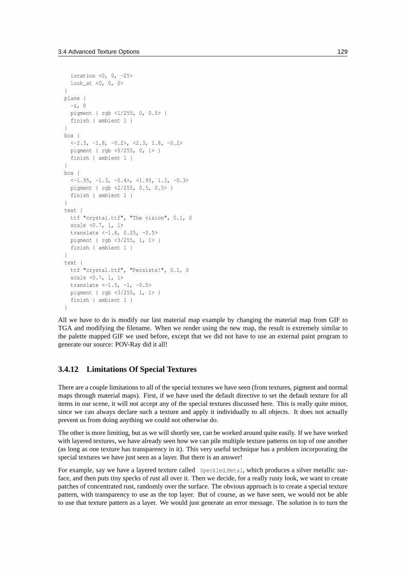
3.4 Advanced Texture Options 129
location <0, 0, -25>look_at <0, 0, 0>
}plane {
-z, 0pigment { rgb <1/255, 0, 0.5> }finish { ambient 1 }
}box {
<-2.3, -1.8, -0.2>, <2.3, 1.8, -0.2>pigment { rgb <0/255, 0, 1> }finish { ambient 1 }
}box {
<-1.95, -1.3, -0.4>, <1.95, 1.3, -0.3>pigment { rgb <2/255, 0.5, 0.5> }finish { ambient 1 }
}text {
ttf "crystal.ttf", "The vision", 0.1, 0scale <0.7, 1, 1>translate <-1.8, 0.25, -0.5>pigment { rgb <3/255, 1, 1> }finish { ambient 1 }
}text {
ttf "crystal.ttf", "Persists!", 0.1, 0scale <0.7, 1, 1>translate <-1.5, -1, -0.5>pigment { rgb <3/255, 1, 1> }finish { ambient 1 }
}
All we have to do is modify our last material map example by changing the material map from GIF toTGA and modifying the filename. When we render using the new map, the result is extremely similar tothe palette mapped GIF we used before, except that we did not have to use an external paint program togenerate our source: POV-Ray did it all!
3.4.12 Limitations Of Special Textures
There are a couple limitations to all of the special textures we have seen (from textures, pigment and normalmaps through material maps). First, if we have used the default directive to set the default texture for allitems in our scene, it will not accept any of the special textures discussed here. This is really quite minor,since we can always declare such a texture and apply it individually to all objects. It does not actuallyprevent us from doing anything we could not otherwise do.
The other is more limiting, but as we will shortly see, can be worked around quite easily. If we have workedwith layered textures, we have already seen how we can pile multiple texture patterns on top of one another(as long as one texture has transparency in it). This very useful technique has a problem incorporating thespecial textures we have just seen as a layer. But there is an answer!
For example, say we have a layered texture calledSpeckled Metal, which produces a silver metallic sur-face, and then puts tiny specks of rust all over it. Then we decide, for a really rusty look, we want to createpatches of concentrated rust, randomly over the surface. The obvious approach is to create a special texturepattern, with transparency to use as the top layer. But of course, as we have seen, we would not be ableto use that texture pattern as a layer. We would just generate an error message. The solution is to turn the
130 Advanced Features
problem inside out, and make our layered texture part of the texture pattern instead, like this
// This part declares a pigment for use// in the rust patch texture pattern#declare Rusty = pigment {
granitecolor_map {
[ 0 rgb <0.2, 0, 0> ][ 1 Brown ]
}frequency 20
}// And this part applies it// Notice that our original layered texture// "Speckled_Metal" is now part of the map#declare Rust_Patches = texture {
bozotexture_map {
[ 0.0 pigment {Rusty} ][ 0.75 Speckled_Metal ][ 1.0 Speckled_Metal ]
}}
And the ultimate effect is the same as if we had layered the rust patches on to the speckled metal anyway.
With the full array of patterns, pigments, normals, finishes, layered and special textures, there is nowpractically nothing we cannot create in the way of amazing textures. An almost infinite number of newpossibilities are just waiting to be created!
3.5 Using Atmospheric Effects
You know you have been raytracing too long when ...... You want to cheat and look at nature’s source code.
– Mark Stock
POV-Ray offers a variety of atmospheric effects, i. e. features that affect the background of the scene or theair by which everything is surrounded.
It is easy to assign a simple color or a complex color pattern to a virtual sky sphere. You can create anythingfrom a cloud free, blue summer sky to a stormy, heavy clouded sky. Even starfields can easily be created.
You can use different kinds of fog to create foggy scenes. Multiple fog layers of different colors can add aneerie touch to your scene.
A much more realistic effect can be created by using an atmosphere, a constant fog that interacts with thelight coming from light sources. Beams of light become visible and objects will cast shadows into the fog.
Last but not least you can add a rainbow to your scene.
3.5.1 The Background
Thebackground feature is used to assign a color to all rays that do not hit any object. This is done in thefollowing way.
camera {location <0, 0, -10>
3.5 Using Atmospheric Effects 131
look_at <0, 0, 0>}background { color rgb <0.2, 0.2, 0.3> }sphere {
0, 1pigment { color rgb <0.8, 0.5, 0.2> }
}
The background color will be visible if a sky sphere is used and if some translucency remains after all skysphere pigment layers are processed.
3.5.2 The Sky Sphere
The sky sphere can be used to easily create a cloud covered sky, a nightly star sky or whatever sky youhave in mind.
In the following examples we will start with a very simple sky sphere that will get more and more complexas we add new features to it.
Creating a Sky with a Color Gradient
Beside the single color sky sphere that is covered with the background feature the simplest sky sphere is acolor gradient. You may have noticed that the color of the sky varies with the angle to the earth’s surfacenormal. If you look straight up the sky normally has a much deeper blue than it has at the horizon.
We want to model this effect using the sky sphere as shown in the sceneskysph1.pov below.
#include "colors.inc"camera {
location <0, 1, -4>look_at <0, 2, 0>angle 80
}light_source { <10, 10, -10> White }sphere {
2*y, 1pigment { color rgb <1, 1, 1> }finish { ambient 0.2 diffuse 0 reflection 0.6 }
}sky_sphere {
pigment {gradient ycolor_map {
[0 color Red][1 color Blue]
}scale 2translate -1
}}
The interesting part is the sky sphere statement. It contains a pigment that describes the look of the skysphere. We want to create a color gradient along the viewing angle measured against the earth’s surfacenormal. Since the ray direction vector is used to calculate the pigment colors we have to use the y-gradient.
The scale and translate transformation are used to map the points derived from the direction vector to theright range. Without those transformations the pattern would be repeated twice on the sky sphere. The
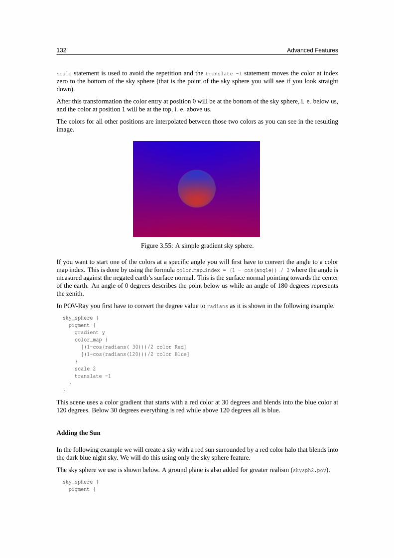
132 Advanced Features
scale statement is used to avoid the repetition and thetranslate -1 statement moves the color at indexzero to the bottom of the sky sphere (that is the point of the sky sphere you will see if you look straightdown).
After this transformation the color entry at position 0 will be at the bottom of the sky sphere, i. e. below us,and the color at position 1 will be at the top, i. e. above us.
The colors for all other positions are interpolated between those two colors as you can see in the resultingimage.
Figure 3.55: A simple gradient sky sphere.
If you want to start one of the colors at a specific angle you will first have to convert the angle to a colormap index. This is done by using the formulacolor map index = (1 - cos(angle)) / 2 where the angle ismeasured against the negated earth’s surface normal. This is the surface normal pointing towards the centerof the earth. An angle of 0 degrees describes the point below us while an angle of 180 degrees representsthe zenith.
In POV-Ray you first have to convert the degree value toradians as it is shown in the following example.
sky_sphere {pigment {
gradient ycolor_map {
[(1-cos(radians( 30)))/2 color Red][(1-cos(radians(120)))/2 color Blue]
}scale 2translate -1
}}
This scene uses a color gradient that starts with a red color at 30 degrees and blends into the blue color at120 degrees. Below 30 degrees everything is red while above 120 degrees all is blue.
Adding the Sun
In the following example we will create a sky with a red sun surrounded by a red color halo that blends intothe dark blue night sky. We will do this using only the sky sphere feature.
The sky sphere we use is shown below. A ground plane is also added for greater realism (skysph2.pov).
sky_sphere {pigment {
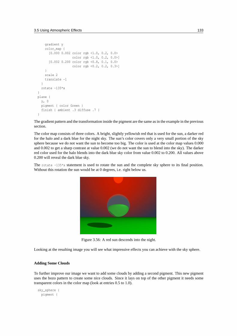
3.5 Using Atmospheric Effects 133
gradient ycolor_map {
[0.000 0.002 color rgb <1.0, 0.2, 0.0>color rgb <1.0, 0.2, 0.0>]
[0.002 0.200 color rgb <0.8, 0.1, 0.0>color rgb <0.2, 0.2, 0.3>]
}scale 2translate -1
}rotate -135*x
}plane {
y, 0pigment { color Green }finish { ambient .3 diffuse .7 }
}
The gradient pattern and the transformation inside the pigment are the same as in the example in the previoussection.
The color map consists of three colors. A bright, slightly yellowish red that is used for the sun, a darker redfor the halo and a dark blue for the night sky. The sun’s color covers only a very small portion of the skysphere because we do not want the sun to become too big. The color is used at the color map values 0.000and 0.002 to get a sharp contrast at value 0.002 (we do not want the sun to blend into the sky). The darkerred color used for the halo blends into the dark blue sky color from value 0.002 to 0.200. All values above0.200 will reveal the dark blue sky.
The rotate -135*x statement is used to rotate the sun and the complete sky sphere to its final position.Without this rotation the sun would be at 0 degrees, i.e. right below us.
Figure 3.56: A red sun descends into the night.
Looking at the resulting image you will see what impressive effects you can achieve with the sky sphere.
Adding Some Clouds
To further improve our image we want to add some clouds by adding a second pigment. This new pigmentuses the bozo pattern to create some nice clouds. Since it lays on top of the other pigment it needs sometransparent colors in the color map (look at entries 0.5 to 1.0).
sky_sphere {pigment {
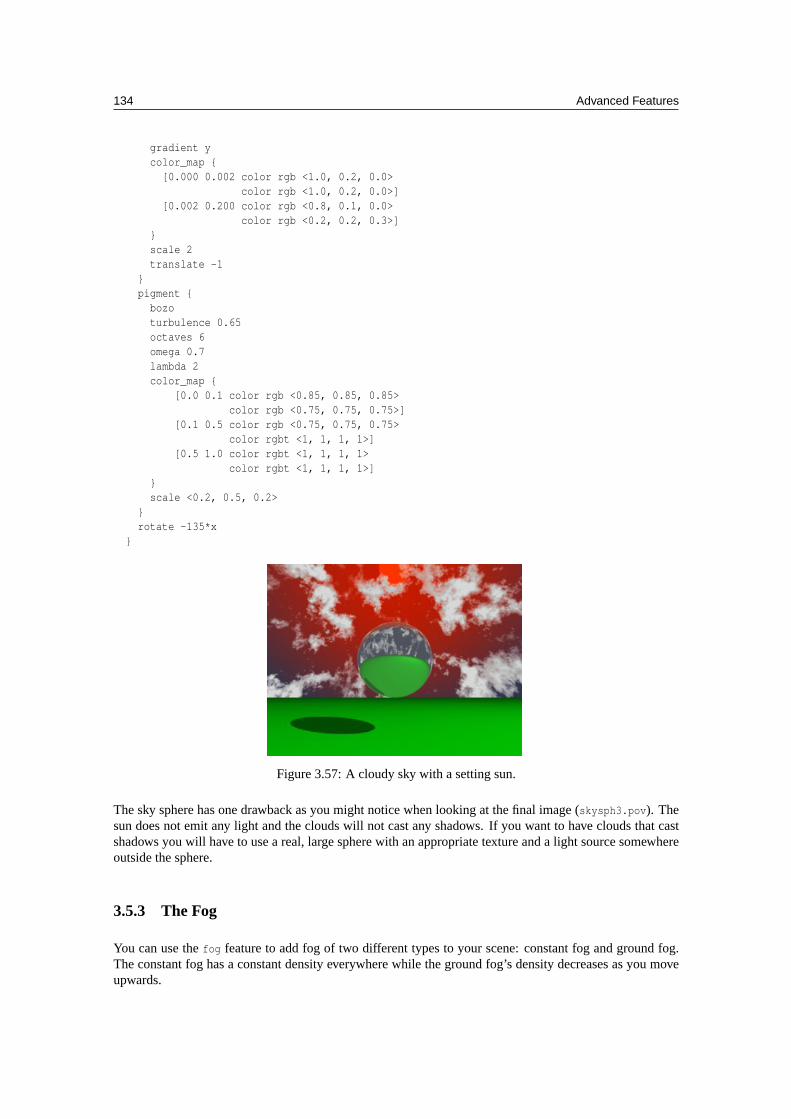
134 Advanced Features
gradient ycolor_map {
[0.000 0.002 color rgb <1.0, 0.2, 0.0>color rgb <1.0, 0.2, 0.0>]
[0.002 0.200 color rgb <0.8, 0.1, 0.0>color rgb <0.2, 0.2, 0.3>]
}scale 2translate -1
}pigment {
bozoturbulence 0.65octaves 6omega 0.7lambda 2color_map {
[0.0 0.1 color rgb <0.85, 0.85, 0.85>color rgb <0.75, 0.75, 0.75>]
[0.1 0.5 color rgb <0.75, 0.75, 0.75>color rgbt <1, 1, 1, 1>]
[0.5 1.0 color rgbt <1, 1, 1, 1>color rgbt <1, 1, 1, 1>]
}scale <0.2, 0.5, 0.2>
}rotate -135*x
}
Figure 3.57: A cloudy sky with a setting sun.
The sky sphere has one drawback as you might notice when looking at the final image (skysph3.pov). Thesun does not emit any light and the clouds will not cast any shadows. If you want to have clouds that castshadows you will have to use a real, large sphere with an appropriate texture and a light source somewhereoutside the sphere.
3.5.3 The Fog
You can use thefog feature to add fog of two different types to your scene: constant fog and ground fog.The constant fog has a constant density everywhere while the ground fog’s density decreases as you moveupwards.
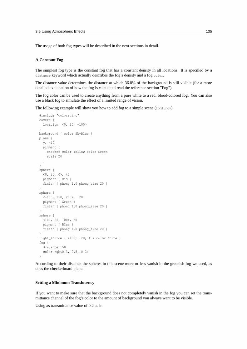
3.5 Using Atmospheric Effects 135
The usage of both fog types will be described in the next sections in detail.
A Constant Fog
The simplest fog type is the constant fog that has a constant density in all locations. It is specified by adistance keyword which actually describes the fog’s density and a fogcolor.
The distance value determines the distance at which 36.8% of the background is still visible (for a moredetailed explanation of how the fog is calculated read the reference section ”Fog”).
The fog color can be used to create anything from a pure white to a red, blood-colored fog. You can alsouse a black fog to simulate the effect of a limited range of vision.
The following example will show you how to add fog to a simple scene (fog1.pov).
#include "colors.inc"camera {
location <0, 20, -100>}background { color SkyBlue }plane {
y, -10pigment {
checker color Yellow color Greenscale 20
}}sphere {
<0, 25, 0>, 40pigment { Red }finish { phong 1.0 phong_size 20 }
}sphere {
<-100, 150, 200>, 20pigment { Green }finish { phong 1.0 phong_size 20 }
}sphere {
<100, 25, 100>, 30pigment { Blue }finish { phong 1.0 phong_size 20 }
}light_source { <100, 120, 40> color White }fog {
distance 150color rgb<0.3, 0.5, 0.2>
}
According to their distance the spheres in this scene more or less vanish in the greenish fog we used, asdoes the checkerboard plane.
Setting a Minimum Translucency
If you want to make sure that the background does not completely vanish in the fog you can set the trans-mittance channel of the fog’s color to the amount of background you always want to be visible.
Using as transmittance value of 0.2 as in
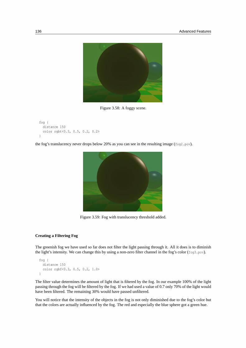
136 Advanced Features
Figure 3.58: A foggy scene.
fog {distance 150color rgbt<0.3, 0.5, 0.2, 0.2>
}
the fog’s translucency never drops below 20% as you can see in the resulting image (fog2.pov).
Figure 3.59: Fog with translucency threshold added.
Creating a Filtering Fog
The greenish fog we have used so far does not filter the light passing through it. All it does is to diminishthe light’s intensity. We can change this by using a non-zero filter channel in the fog’s color (fog3.pov).
fog {distance 150color rgbf<0.3, 0.5, 0.2, 1.0>
}
The filter value determines the amount of light that is filtered by the fog. In our example 100% of the lightpassing through the fog will be filtered by the fog. If we had used a value of 0.7 only 70% of the light wouldhave been filtered. The remaining 30% would have passed unfiltered.
You will notice that the intensity of the objects in the fog is not only diminished due to the fog’s color butthat the colors are actually influenced by the fog. The red and especially the blue sphere got a green hue.
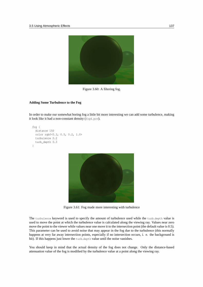
3.5 Using Atmospheric Effects 137
Figure 3.60: A filtering fog.
Adding Some Turbulence to the Fog
In order to make our somewhat boring fog a little bit more interesting we can add some turbulence, makingit look like it had a non-constant density (fog4.pov).
fog {distance 150color rgbf<0.3, 0.5, 0.2, 1.0>turbulence 0.2turb_depth 0.3
}
Figure 3.61: Fog made more interesting with turbulence
The turbulence keyword is used to specify the amount of turbulence used while theturb depth value isused to move the point at which the turbulence value is calculated along the viewing ray. Values near zeromove the point to the viewer while values near one move it to the intersection point (the default value is 0.5).This parameter can be used to avoid noise that may appear in the fog due to the turbulence (this normallyhappens at very far away intersection points, especially if no intersection occurs, i. e. the background ishit). If this happens just lower theturb depth value until the noise vanishes.
You should keep in mind that the actual density of the fog does not change. Only the distance-basedattenuation value of the fog is modified by the turbulence value at a point along the viewing ray.
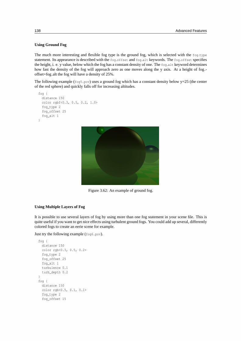
138 Advanced Features
Using Ground Fog
The much more interesting and flexible fog type is the ground fog, which is selected with thefog type
statement. Its appearance is described with thefog offset andfog alt keywords. Thefog offset specifiesthe height, i. e. y value, below which the fog has a constant density of one. Thefog alt keyword determineshow fast the density of the fog will approach zero as one moves along the y axis. At a height of fog-offset+fogalt the fog will have a density of 25%.
The following example (fog5.pov) uses a ground fog which has a constant density below y=25 (the centerof the red sphere) and quickly falls off for increasing altitudes.
fog {distance 150color rgbf<0.3, 0.5, 0.2, 1.0>fog_type 2fog_offset 25fog_alt 1
}
Figure 3.62: An example of ground fog.
Using Multiple Layers of Fog
It is possible to use several layers of fog by using more than one fog statement in your scene file. This isquite useful if you want to get nice effects using turbulent ground fogs. You could add up several, differentlycolored fogs to create an eerie scene for example.
Just try the following example (fog6.pov).
fog {distance 150color rgb<0.3, 0.5, 0.2>fog_type 2fog_offset 25fog_alt 1turbulence 0.1turb_depth 0.2
}fog {
distance 150color rgb<0.5, 0.1, 0.1>fog_type 2fog_offset 15
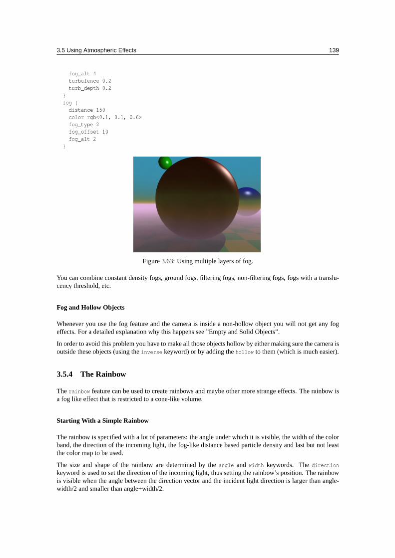
3.5 Using Atmospheric Effects 139
fog_alt 4turbulence 0.2turb_depth 0.2
}fog {
distance 150color rgb<0.1, 0.1, 0.6>fog_type 2fog_offset 10fog_alt 2
}
Figure 3.63: Using multiple layers of fog.
You can combine constant density fogs, ground fogs, filtering fogs, non-filtering fogs, fogs with a translu-cency threshold, etc.
Fog and Hollow Objects
Whenever you use the fog feature and the camera is inside a non-hollow object you will not get any fogeffects. For a detailed explanation why this happens see ”Empty and Solid Objects”.
In order to avoid this problem you have to make all those objects hollow by either making sure the camera isoutside these objects (using theinverse keyword) or by adding thehollow to them (which is much easier).
3.5.4 The Rainbow
Therainbow feature can be used to create rainbows and maybe other more strange effects. The rainbow isa fog like effect that is restricted to a cone-like volume.
Starting With a Simple Rainbow
The rainbow is specified with a lot of parameters: the angle under which it is visible, the width of the colorband, the direction of the incoming light, the fog-like distance based particle density and last but not leastthe color map to be used.
The size and shape of the rainbow are determined by theangle and width keywords. Thedirectionkeyword is used to set the direction of the incoming light, thus setting the rainbow’s position. The rainbowis visible when the angle between the direction vector and the incident light direction is larger than angle-width/2 and smaller than angle+width/2.
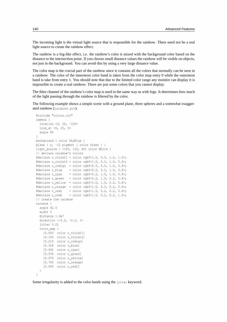
140 Advanced Features
The incoming light is the virtual light source that is responsible for the rainbow. There need not be a reallight source to create the rainbow effect.
The rainbow is a fog-like effect, i.e. the rainbow’s color is mixed with the background color based on thedistance to the intersection point. If you choose small distance values the rainbow will be visible on objects,not just in the background. You can avoid this by using a very large distance value.
The color map is the crucial part of the rainbow since it contains all the colors that normally can be seen ina rainbow. The color of the innermost color band is taken from the color map entry 0 while the outermostband is take from entry 1. You should note that due to the limited color range any monitor can display it isimpossible to create a real rainbow. There are just some colors that you cannot display.
The filter channel of the rainbow’s color map is used in the same way as with fogs. It determines how muchof the light passing through the rainbow is filtered by the color.
The following example shows a simple scene with a ground plane, three spheres and a somewhat exagger-ated rainbow (rainbow1.pov).
#include "colors.inc"camera {
location <0, 20, -100>look_at <0, 25, 0>angle 80
}background { color SkyBlue }plane { y, -10 pigment { color Green } }light_source { <100, 120, 40> color White }// declare rainbow’s colors#declare r_violet1 = color rgbf<1.0, 0.5, 1.0, 1.0>;#declare r_violet2 = color rgbf<1.0, 0.5, 1.0, 0.8>;#declare r_indigo = color rgbf<0.5, 0.5, 1.0, 0.8>;#declare r_blue = color rgbf<0.2, 0.2, 1.0, 0.8>;#declare r_cyan = color rgbf<0.2, 1.0, 1.0, 0.8>;#declare r_green = color rgbf<0.2, 1.0, 0.2, 0.8>;#declare r_yellow = color rgbf<1.0, 1.0, 0.2, 0.8>;#declare r_orange = color rgbf<1.0, 0.5, 0.2, 0.8>;#declare r_red1 = color rgbf<1.0, 0.2, 0.2, 0.8>;#declare r_red2 = color rgbf<1.0, 0.2, 0.2, 1.0>;// create the rainbowrainbow {
angle 42.5width 5distance 1.0e7direction <-0.2, -0.2, 1>jitter 0.01color_map {
[0.000 color r_violet1][0.100 color r_violet2][0.214 color r_indigo][0.328 color r_blue][0.442 color r_cyan][0.556 color r_green][0.670 color r_yellow][0.784 color r_orange][0.900 color r_red1]
}}
Some irregularity is added to the color bands using thejitter keyword.
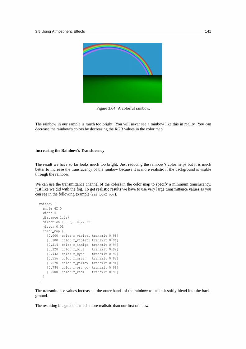
3.5 Using Atmospheric Effects 141
Figure 3.64: A colorful rainbow.
The rainbow in our sample is much too bright. You will never see a rainbow like this in reality. You candecrease the rainbow’s colors by decreasing the RGB values in the color map.
Increasing the Rainbow’s Translucency
The result we have so far looks much too bright. Just reducing the rainbow’s color helps but it is muchbetter to increase the translucency of the rainbow because it is more realistic if the background is visiblethrough the rainbow.
We can use the transmittance channel of the colors in the color map to specify a minimum translucency,just like we did with the fog. To get realistic results we have to use very large transmittance values as youcan see in the following example (rainbow2.pov).
rainbow {angle 42.5width 5distance 1.0e7direction <-0.2, -0.2, 1>jitter 0.01color_map {
[0.000 color r_violet1 transmit 0.98][0.100 color r_violet2 transmit 0.96][0.214 color r_indigo transmit 0.94][0.328 color r_blue transmit 0.92][0.442 color r_cyan transmit 0.90][0.556 color r_green transmit 0.92][0.670 color r_yellow transmit 0.94][0.784 color r_orange transmit 0.96][0.900 color r_red1 transmit 0.98]
}}
The transmittance values increase at the outer bands of the rainbow to make it softly blend into the back-ground.
The resulting image looks much more realistic than our first rainbow.
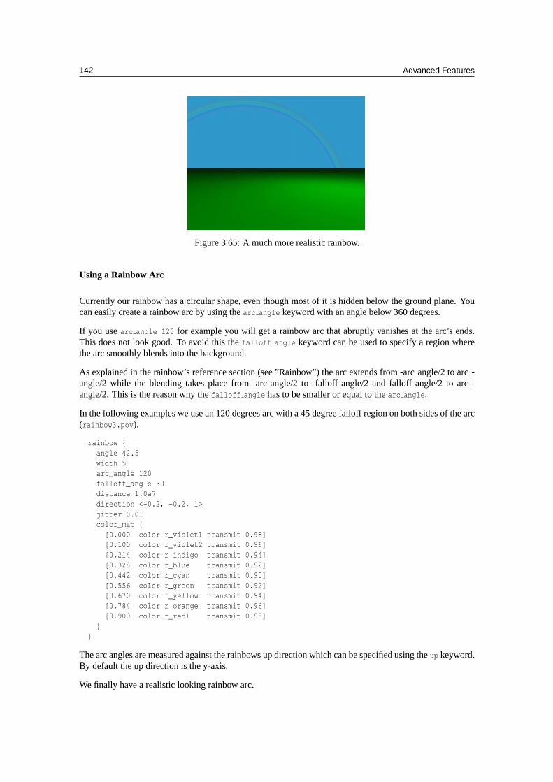
142 Advanced Features
Figure 3.65: A much more realistic rainbow.
Using a Rainbow Arc
Currently our rainbow has a circular shape, even though most of it is hidden below the ground plane. Youcan easily create a rainbow arc by using thearc angle keyword with an angle below 360 degrees.
If you usearc angle 120 for example you will get a rainbow arc that abruptly vanishes at the arc’s ends.This does not look good. To avoid this thefalloff angle keyword can be used to specify a region wherethe arc smoothly blends into the background.
As explained in the rainbow’s reference section (see ”Rainbow”) the arc extends from -arcangle/2 to arc-angle/2 while the blending takes place from -arcangle/2 to -falloffangle/2 and falloffangle/2 to arc-angle/2. This is the reason why thefalloff angle has to be smaller or equal to thearc angle.
In the following examples we use an 120 degrees arc with a 45 degree falloff region on both sides of the arc(rainbow3.pov).
rainbow {angle 42.5width 5arc_angle 120falloff_angle 30distance 1.0e7direction <-0.2, -0.2, 1>jitter 0.01color_map {
[0.000 color r_violet1 transmit 0.98][0.100 color r_violet2 transmit 0.96][0.214 color r_indigo transmit 0.94][0.328 color r_blue transmit 0.92][0.442 color r_cyan transmit 0.90][0.556 color r_green transmit 0.92][0.670 color r_yellow transmit 0.94][0.784 color r_orange transmit 0.96][0.900 color r_red1 transmit 0.98]
}}
The arc angles are measured against the rainbows up direction which can be specified using theup keyword.By default the up direction is the y-axis.
We finally have a realistic looking rainbow arc.
3.6 Simple Media Tutorial 143
Figure 3.66: A rainbow arc.
3.6 Simple Media Tutorial
Media in POV-Ray is a very versatile feature and can be used for a very diverse set of special effects suchas glows, smoke, dust, fog, etc. However, due to its versatility, media is not one of the easiest and simplestfeatures of POV-Ray and often requires experience for getting things to look good.
3.6.1 Types of media
There are three types of media in POV-Ray: Emitting, absorbing and scattering. They have the followingproperties:
• Emitting: This is an additive media, which is handled as if it only emits light (note: it does not emitlight to its surroundings like alight source does; this just describes how it affects the rays goingthrough it). That is, the color of the media is added to the color of the ray passing through it. Lightsources do not have any effect at all in it (ie. it does not affect shadows in any way).
• Absorbing: This is a substractive media. This media substracts (absorbs) its coloration from the raypassing through it. Light sources are taken into account only in the shadow of the media (that is,absorbing media casts a shadow).
• Scattering: This is the most advanced media type as it fully takes into account light passing throughit. That is, this media is lit by light sources (and thus, for example, nearby objects can cast shadowsinto the scattering media).
Emitting and absorbing medias are the simplest and thus fastest ones. Emitting media can be used for thingslike glows, lasers, sparkles and similar light-emitting effects. Absorbing media can be used for things likesmoke and fog (the difference between thefog feature of POV-Ray is that the density of an absorbing mediacan be modified by a pattern and the media can be contained inside an object).
Scattering media is the more advanced and slower type. It is somewhat similar to absorbing media exceptthat it is fully lit by light sources. This can be used for smoke or fog with visible lightbeams and shadows.
3.6.2 Some media concepts
Media can be global to the whole universe, or it can be contained by an object. In the latter case the mediais defined in theinterior block of the object definition.
144 Advanced Features
For an object to be able to contain media (or to allow media from other objects or the global media insideitself) it has to be defined ashollow (a common mistake is to forget adding this keyword). If an object withno media should not allow media inside itself (eg. a solid glass ball), thenhollow should not be defined forthat object.
If media is defined in theinterior of an object or as a global media it will have a constant density throughoutthe object/universe. However, a density pattern can be specified for non-uniform media. Also all kinds oftransformations can be applied to the media. This is specially useful for various effects (such as smoke withcertain shape).
3.6.3 Simple media examples
Emitting media
Let’s start with a very simple scene showing an emitting media using a spherical density map. Emittingmedia is used with theemission keyword followed by a color value. This color value tells the overall colorof the media:
global_settings { assumed_gamma 1 }background { rgb 1 }camera { location <3,4,-5>*.8 look_at 0 angle 35 }light_source { <20,40,10>, 1 }
box // floor{ <-1.5,-1.01,-1.5>, <1.5,-1.2,1.5>
pigment { checker rgb 0.75, rgb 0.25 scale 0.2 }}
sphere // transparent sphere containing media{ 0,1 pigment { rgbt 1 } hollow
interior{ media
{ emission 1density{ spherical density_map
{ [0 rgb 0][0.4 rgb <1,0,0>][0.8 rgb <1,1,0>][1 rgb 1]
}}
}}
}
Note that thespherical pattern gets values from 0 in the outer surface of a unit sphere to 1 in the origin(that is, the density with the index value 1 will be the density at the center of the media).
The color values in the density map tell what color the media is emitting at a certain point in the pattern.That is, for example when the pattern gets the value 0.4, the media will be completely red at that place. Ifthe color is<0,0,0>, it means that the media does not emit any light at all in that location.
Note that the density map colors are multiplied by the color given with theemission keyword; since 1 isused in this case, the density map colors are not affected.
Thus, this will give us a media with a bright white center which fades to yellow and red at the outer limitsof the unit sphere:
3.6 Simple Media Tutorial 145
Figure 3.67: Simple emitting media example
As you can see from the image, the emitting media is invisible against white background. This is due to itsadditive nature (any color added to pure white gives pure white). In fact, emitting media gives usually bestresults for dark backgrounds.
Absorbing media
Modifying the previous example to use absorbing media is rather simple: Simply change theemission
keyword forabsorption. However, the colors we used above are not very illustrative for absorbing media,so let’s change them a bit like this:
media{ absorption 1
density{ spherical density_map
{ [0 rgb 0][0.4 rgb 0][0.5 rgb <0,0.5,1>][1 rgb <0,1,1>]
}}
}
Figure 3.68: Simple absorbing media example
The feature which we immediately notice in the image is that the media seems to be inverted from the colorsspecified in the density map: Blueish colors were specified in the map, but the image shows a reddish media.
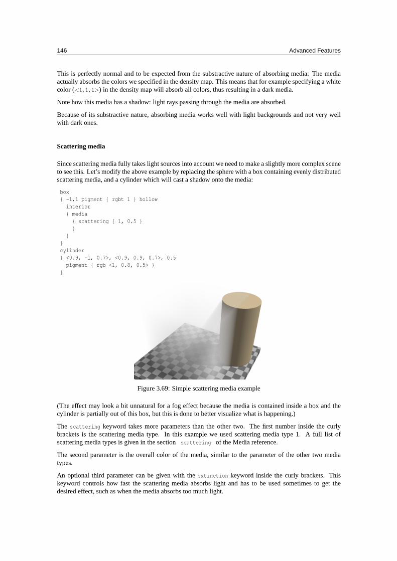
146 Advanced Features
This is perfectly normal and to be expected from the substractive nature of absorbing media: The mediaactually absorbs the colors we specified in the density map. This means that for example specifying a whitecolor (<1,1,1>) in the density map will absorb all colors, thus resulting in a dark media.
Note how this media has a shadow: light rays passing through the media are absorbed.
Because of its substractive nature, absorbing media works well with light backgrounds and not very wellwith dark ones.
Scattering media
Since scattering media fully takes light sources into account we need to make a slightly more complex sceneto see this. Let’s modify the above example by replacing the sphere with a box containing evenly distributedscattering media, and a cylinder which will cast a shadow onto the media:
box{ -1,1 pigment { rgbt 1 } hollow
interior{ media
{ scattering { 1, 0.5 }}
}}cylinder{ <0.9, -1, 0.7>, <0.9, 0.9, 0.7>, 0.5
pigment { rgb <1, 0.8, 0.5> }}
Figure 3.69: Simple scattering media example
(The effect may look a bit unnatural for a fog effect because the media is contained inside a box and thecylinder is partially out of this box, but this is done to better visualize what is happening.)
The scattering keyword takes more parameters than the other two. The first number inside the curlybrackets is the scattering media type. In this example we used scattering media type 1. A full list ofscattering media types is given in the sectionscattering of the Media reference.
The second parameter is the overall color of the media, similar to the parameter of the other two mediatypes.
An optional third parameter can be given with theextinction keyword inside the curly brackets. Thiskeyword controls how fast the scattering media absorbs light and has to be used sometimes to get thedesired effect, such as when the media absorbs too much light.
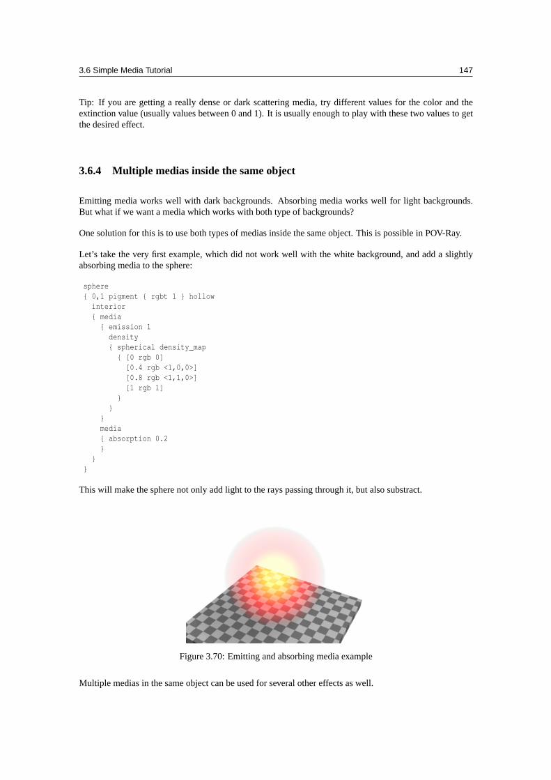
3.6 Simple Media Tutorial 147
Tip: If you are getting a really dense or dark scattering media, try different values for the color and theextinction value (usually values between 0 and 1). It is usually enough to play with these two values to getthe desired effect.
3.6.4 Multiple medias inside the same object
Emitting media works well with dark backgrounds. Absorbing media works well for light backgrounds.But what if we want a media which works with both type of backgrounds?
One solution for this is to use both types of medias inside the same object. This is possible in POV-Ray.
Let’s take the very first example, which did not work well with the white background, and add a slightlyabsorbing media to the sphere:
sphere{ 0,1 pigment { rgbt 1 } hollow
interior{ media
{ emission 1density{ spherical density_map
{ [0 rgb 0][0.4 rgb <1,0,0>][0.8 rgb <1,1,0>][1 rgb 1]
}}
}media{ absorption 0.2}
}}
This will make the sphere not only add light to the rays passing through it, but also substract.
Figure 3.70: Emitting and absorbing media example
Multiple medias in the same object can be used for several other effects as well.
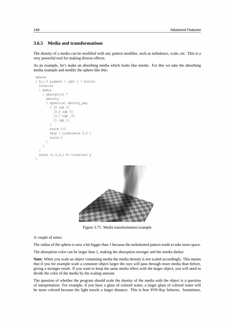
148 Advanced Features
3.6.5 Media and transformations
The density of a media can be modified with any pattern modifier, such as turbulence, scale, etc. This is avery powerful tool for making diverse effects.
As an example, let’s make an absorbing media which looks like smoke. For this we take the absorbingmedia example and modify the sphere like this:
sphere{ 0,1.5 pigment { rgbt 1 } hollow
interior{ media
{ absorption 7density{ spherical density_map
{ [0 rgb 0][0.5 rgb 0][0.7 rgb .5][1 rgb 1]
}scale 1/2warp { turbulence 0.5 }scale 2
}}
}scale <1.5,6,1.5> translate y
}
Figure 3.71: Media transformation example
A couple of notes:
The radius of the sphere is now a bit bigger than 1 because the turbulented pattern tends to take more space.
The absorption color can be larger than 1, making the absorption stronger and the smoke darker.
Note: When you scale an object containing media the media density is not scaled accordingly. This meansthat if you for example scale a container object larger the rays will pass through more media than before,giving a stronger result. If you want to keep the same media effect with the larger object, you will need todivide the color of the media by the scaling amount.
The question of whether the program should scale the density of the media with the object is a questionof interpretation: For example, if you have a glass of colored water, a larger glass of colored water willbe more colored because the light travels a larger distance. This is how POV-Ray behaves. Sometimes,
3.6 Simple Media Tutorial 149
however, the object needs to be scaled so that the media does not change; in this case the media color needsto be scaled inversely.
3.6.6 A more advanced example of scattering media
For a bit more advanced example of scattering media, let’s make a room with a window and a light sourceilluminating from outside the room. The room contains scattering media, thus making the light beamcoming through the window visible.
global_settings { assumed_gamma 1 }camera { location <14.9, 1, -8> look_at -z angle 70 }light_source { <10,100,150>, 1 }background { rgb <0.3, 0.6, 0.9> }
// A dim light source inside the room which does not// interact with media so that we can see the room:light_source { <14, -5, 2>, 0.5 media_interaction off }
// Roomunion{ difference
{ box { <-11, -7, -11>, <16, 7, 10.5> }box { <-10, -6, -10>, <15, 6, 10> }box { <-4, -2, 9.9>, <2, 3, 10.6> }
}box { <-1.25, -2, 10>, <-0.75, 3, 10.5> }box { <-4, 0.25, 10>, <2, 0.75, 10.5> }pigment { rgb 1 }
}
// Scattering media box:box{ <-5, -6.5, -10.5>, <3, 6.5, 10.25>
pigment { rgbt 1 } hollowinterior{ media
{ scattering { 1, 0.07 extinction 0.01 }samples 30,100
}}
}
As suggested previously, the scattering color and extinction values were adjusted until the image lookedgood. In this kind of scene usually very small values are needed.
Note how the container box is quite smaller than the room itself. Container boxes should always be sized asminimally as possible. If the box were as big as the room much higher values forsamples would be neededfor a good result, thus resulting in a much slower rendering.
3.6.7 Media and photons
The photon mapping technique can be used in POV-Ray for making stunningly beautiful images with lightreflecting and refracting from objects. By default, however, reflected and refracted light does not affectmedia. Making photons interact with media can be turned on with themedia keyword in thephotons blockinsideglobal settings.
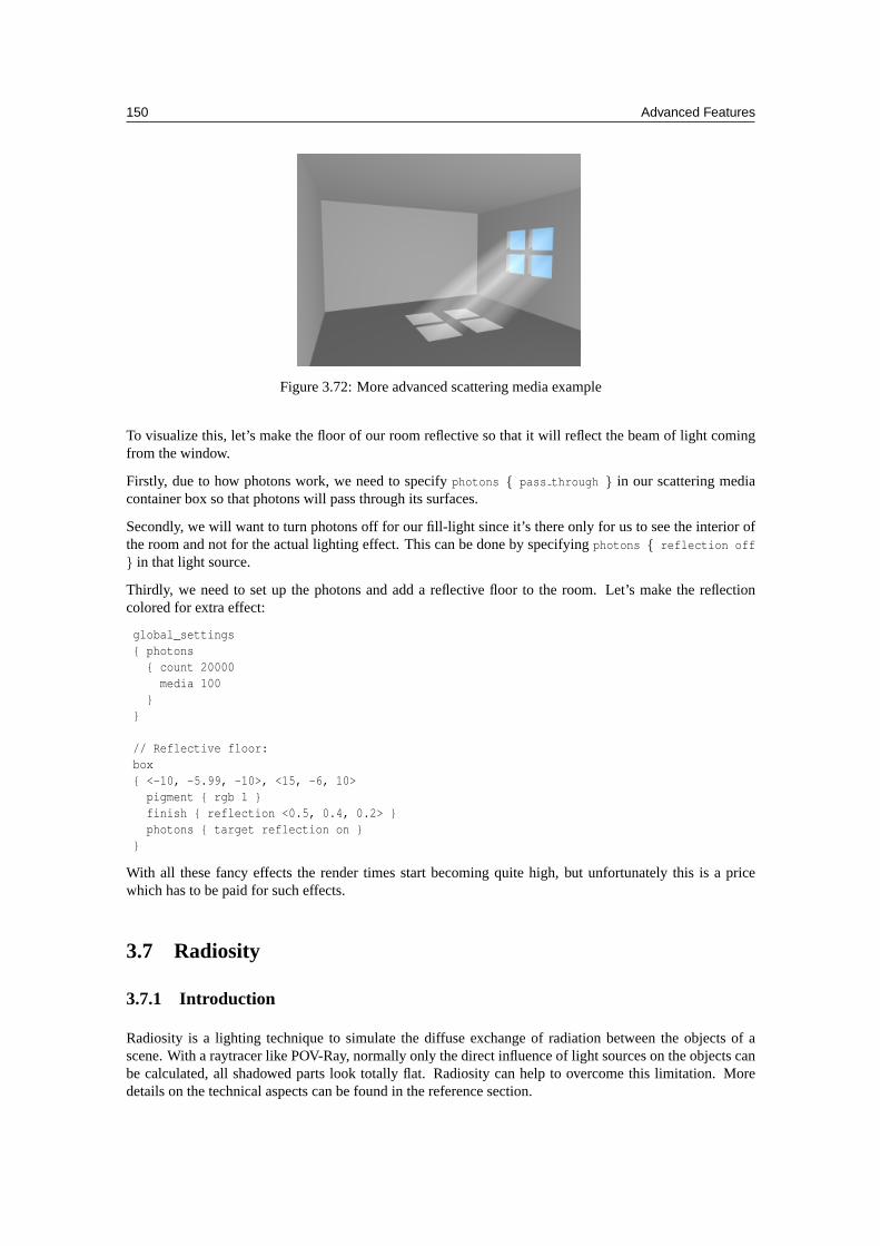
150 Advanced Features
Figure 3.72: More advanced scattering media example
To visualize this, let’s make the floor of our room reflective so that it will reflect the beam of light comingfrom the window.
Firstly, due to how photons work, we need to specifyphotons { pass through } in our scattering mediacontainer box so that photons will pass through its surfaces.
Secondly, we will want to turn photons off for our fill-light since it’s there only for us to see the interior ofthe room and not for the actual lighting effect. This can be done by specifyingphotons { reflection off
} in that light source.
Thirdly, we need to set up the photons and add a reflective floor to the room. Let’s make the reflectioncolored for extra effect:
global_settings{ photons
{ count 20000media 100
}}
// Reflective floor:box{ <-10, -5.99, -10>, <15, -6, 10>
pigment { rgb 1 }finish { reflection <0.5, 0.4, 0.2> }photons { target reflection on }
}
With all these fancy effects the render times start becoming quite high, but unfortunately this is a pricewhich has to be paid for such effects.
3.7 Radiosity
3.7.1 Introduction
Radiosity is a lighting technique to simulate the diffuse exchange of radiation between the objects of ascene. With a raytracer like POV-Ray, normally only the direct influence of light sources on the objects canbe calculated, all shadowed parts look totally flat. Radiosity can help to overcome this limitation. Moredetails on the technical aspects can be found in the reference section.
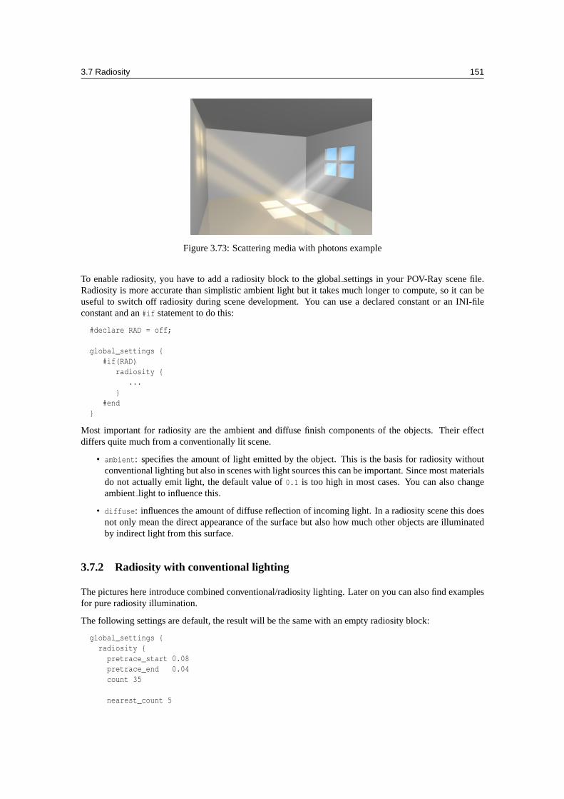
3.7 Radiosity 151
Figure 3.73: Scattering media with photons example
To enable radiosity, you have to add a radiosity block to the globalsettings in your POV-Ray scene file.Radiosity is more accurate than simplistic ambient light but it takes much longer to compute, so it can beuseful to switch off radiosity during scene development. You can use a declared constant or an INI-fileconstant and an#if statement to do this:
#declare RAD = off;
global_settings {#if(RAD)
radiosity {...
}#end
}
Most important for radiosity are the ambient and diffuse finish components of the objects. Their effectdiffers quite much from a conventionally lit scene.
• ambient: specifies the amount of light emitted by the object. This is the basis for radiosity withoutconventional lighting but also in scenes with light sources this can be important. Since most materialsdo not actually emit light, the default value of0.1 is too high in most cases. You can also changeambientlight to influence this.
• diffuse: influences the amount of diffuse reflection of incoming light. In a radiosity scene this doesnot only mean the direct appearance of the surface but also how much other objects are illuminatedby indirect light from this surface.
3.7.2 Radiosity with conventional lighting
The pictures here introduce combined conventional/radiosity lighting. Later on you can also find examplesfor pure radiosity illumination.
The following settings are default, the result will be the same with an empty radiosity block:
global_settings {radiosity {
pretrace_start 0.08pretrace_end 0.04count 35
nearest_count 5
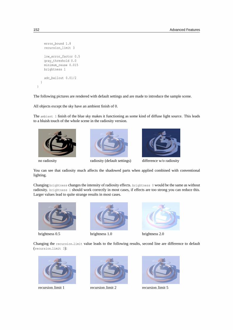
152 Advanced Features
error_bound 1.8recursion_limit 3
low_error_factor 0.5gray_threshold 0.0minimum_reuse 0.015brightness 1
adc_bailout 0.01/2}
}
The following pictures are rendered with default settings and are made to introduce the sample scene.
All objects except the sky have an ambient finish of 0.
Theambient 1 finish of the blue sky makes it functioning as some kind of diffuse light source. This leadsto a bluish touch of the whole scene in the radiosity version.
no radiosity radiosity (default settings) difference w/o radiosity
You can see that radiosity much affects the shadowed parts when applied combined with conventionallighting.
Changingbrightness changes the intensity of radiosity effects.brightness 0 would be the same as withoutradiosity. brightness 1 should work correctly in most cases, if effects are too strong you can reduce this.Larger values lead to quite strange results in most cases.
brightness 0.5 brightness 1.0 brightness 2.0
Changing therecursion limit value leads to the following results, second line are difference to default(recursion limit 3):
recursionlimit 1 recursionlimit 2 recursionlimit 5
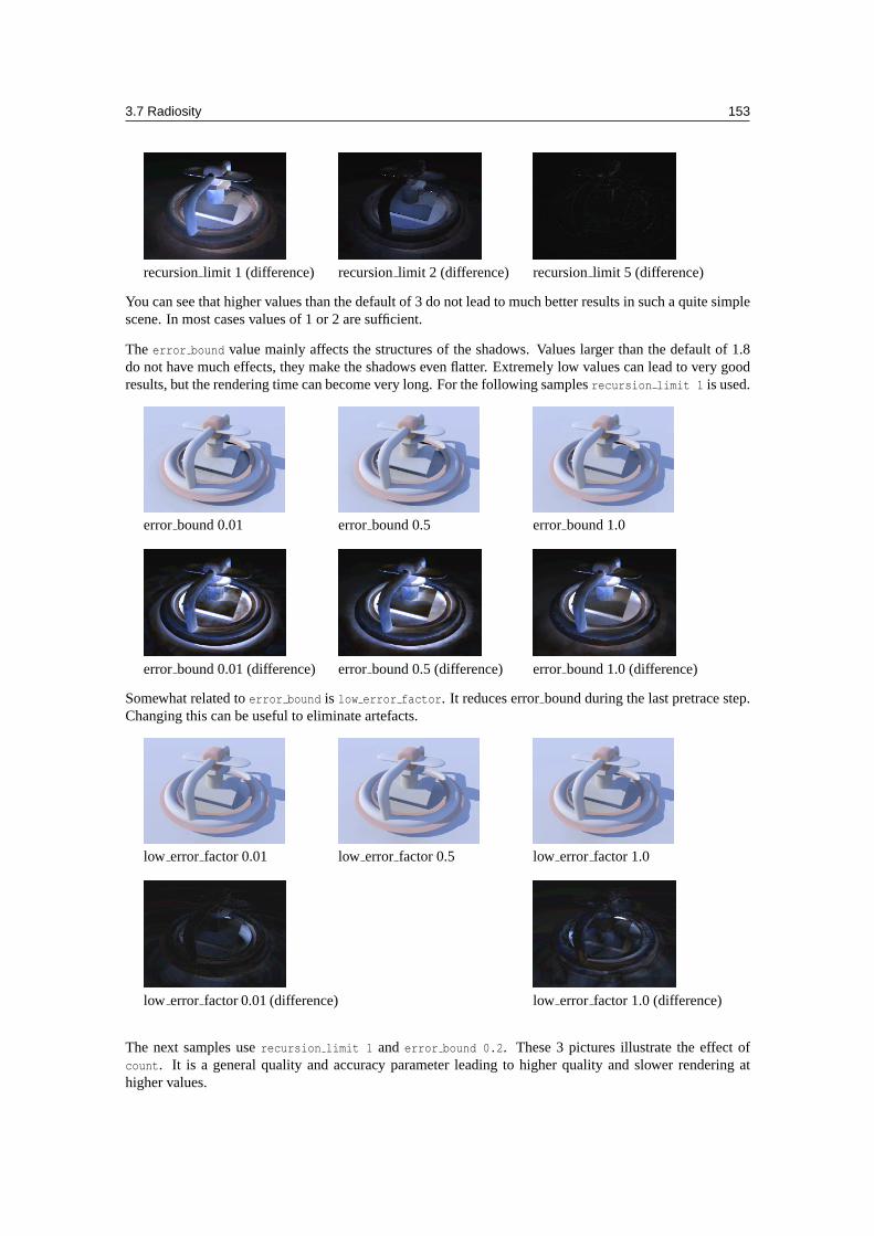
3.7 Radiosity 153
recursionlimit 1 (difference) recursionlimit 2 (difference) recursionlimit 5 (difference)
You can see that higher values than the default of 3 do not lead to much better results in such a quite simplescene. In most cases values of 1 or 2 are sufficient.
Theerror bound value mainly affects the structures of the shadows. Values larger than the default of 1.8do not have much effects, they make the shadows even flatter. Extremely low values can lead to very goodresults, but the rendering time can become very long. For the following samplesrecursion limit 1 is used.
error bound 0.01 error bound 0.5 error bound 1.0
error bound 0.01 (difference) error bound 0.5 (difference) error bound 1.0 (difference)
Somewhat related toerror bound is low error factor. It reduces errorbound during the last pretrace step.Changing this can be useful to eliminate artefacts.
low error factor 0.01 low error factor 0.5 low error factor 1.0
low error factor 0.01 (difference) low error factor 1.0 (difference)
The next samples userecursion limit 1 anderror bound 0.2. These 3 pictures illustrate the effect ofcount. It is a general quality and accuracy parameter leading to higher quality and slower rendering athigher values.
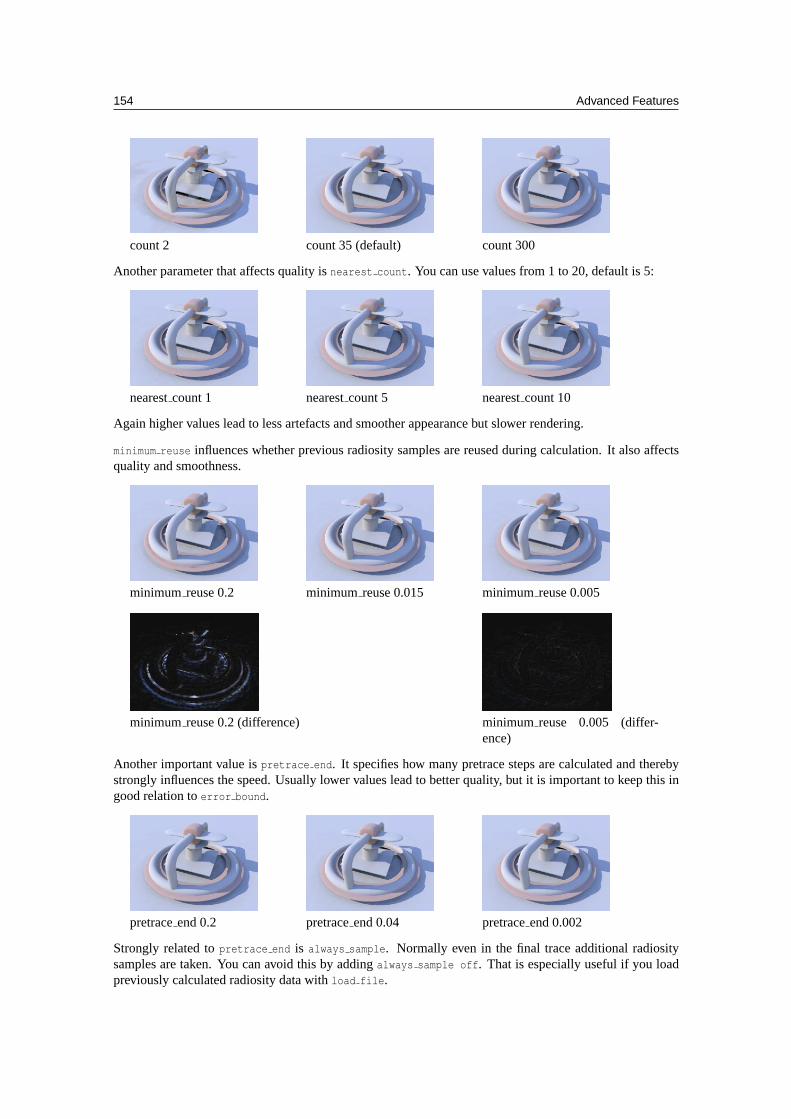
154 Advanced Features
count 2 count 35 (default) count 300
Another parameter that affects quality isnearest count. You can use values from 1 to 20, default is 5:
nearestcount 1 nearestcount 5 nearestcount 10
Again higher values lead to less artefacts and smoother appearance but slower rendering.
minimum reuse influences whether previous radiosity samples are reused during calculation. It also affectsquality and smoothness.
minimum reuse 0.2 minimum reuse 0.015 minimum reuse 0.005
minimum reuse 0.2 (difference) minimum reuse 0.005 (differ-ence)
Another important value ispretrace end. It specifies how many pretrace steps are calculated and therebystrongly influences the speed. Usually lower values lead to better quality, but it is important to keep this ingood relation toerror bound.
pretraceend 0.2 pretraceend 0.04 pretraceend 0.002
Strongly related topretrace end is always sample. Normally even in the final trace additional radiositysamples are taken. You can avoid this by addingalways sample off. That is especially useful if you loadpreviously calculated radiosity data withload file.
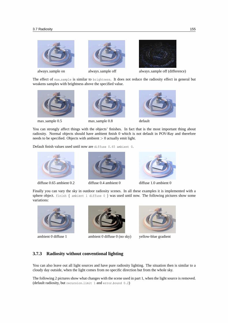
3.7 Radiosity 155
alwayssample on alwayssample off alwayssample off (difference)
The effect ofmax sample is similar tobrightness. It does not reduce the radiosity effect in general butweakens samples with brightness above the specified value.
max sample 0.5 max sample 0.8 default
You can strongly affect things with the objects’ finishes. In fact that is the most important thing aboutradiosity. Normal objects should have ambient finish 0 which is not default in POV-Ray and thereforeneeds to be specified. Objects with ambient> 0 actually emit light.
Default finish values used until now arediffuse 0.65 ambient 0.
diffuse 0.65 ambient 0.2 diffuse 0.4 ambient 0 diffuse 1.0 ambient 0
Finally you can vary the sky in outdoor radiosity scenes. In all these examples it is implemented with asphere object.finish { ambient 1 diffuse 0 } was used until now. The following pictures show somevariations:
ambient 0 diffuse 1 ambient 0 diffuse 0 (no sky) yellow-blue gradient
3.7.3 Radiosity without conventional lighting
You can also leave out all light sources and have pure radiosity lighting. The situation then is similar to acloudy day outside, when the light comes from no specific direction but from the whole sky.
The following 2 pictures show what changes with the scene used in part 1, when the light source is removed.(default radiosity, butrecursion limit 1 anderror bound 0.2)
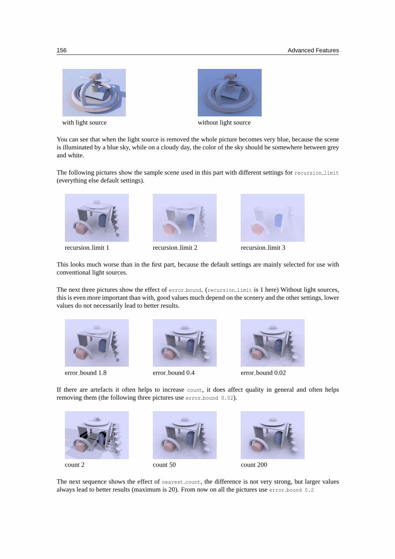
156 Advanced Features
with light source without light source
You can see that when the light source is removed the whole picture becomes very blue, because the sceneis illuminated by a blue sky, while on a cloudy day, the color of the sky should be somewhere between greyand white.
The following pictures show the sample scene used in this part with different settings forrecursion limit
(everything else default settings).
recursionlimit 1 recursionlimit 2 recursionlimit 3
This looks much worse than in the first part, because the default settings are mainly selected for use withconventional light sources.
The next three pictures show the effect oferror bound. (recursion limit is 1 here) Without light sources,this is even more important than with, good values much depend on the scenery and the other settings, lowervalues do not necessarily lead to better results.
error bound 1.8 error bound 0.4 error bound 0.02
If there are artefacts it often helps to increasecount, it does affect quality in general and often helpsremoving them (the following three pictures useerror bound 0.02).
count 2 count 50 count 200
The next sequence shows the effect ofnearest count, the difference is not very strong, but larger valuesalways lead to better results (maximum is 20). From now on all the pictures useerror bound 0.2
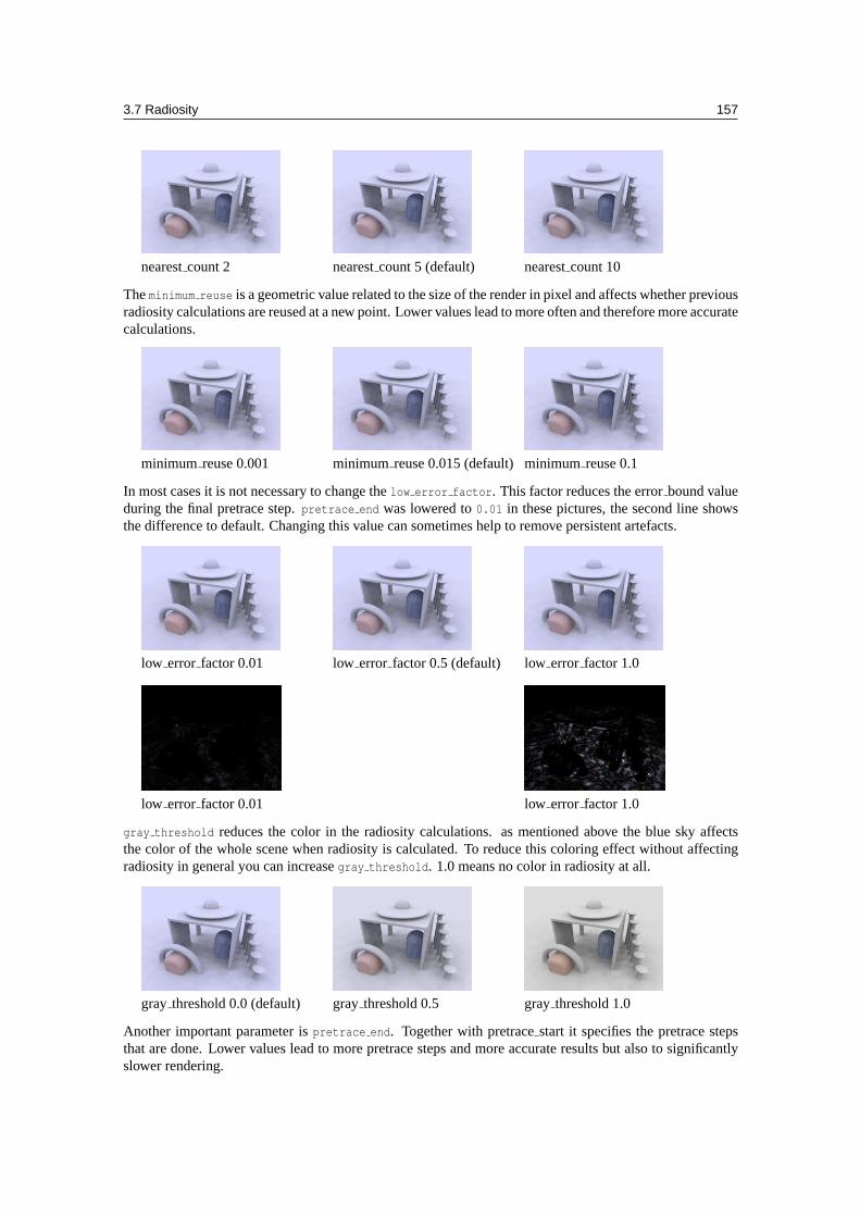
3.7 Radiosity 157
nearestcount 2 nearestcount 5 (default) nearestcount 10
Theminimum reuse is a geometric value related to the size of the render in pixel and affects whether previousradiosity calculations are reused at a new point. Lower values lead to more often and therefore more accuratecalculations.
minimum reuse 0.001 minimum reuse 0.015 (default)minimum reuse 0.1
In most cases it is not necessary to change thelow error factor. This factor reduces the errorbound valueduring the final pretrace step.pretrace end was lowered to0.01 in these pictures, the second line showsthe difference to default. Changing this value can sometimes help to remove persistent artefacts.
low error factor 0.01 low error factor 0.5 (default) low error factor 1.0
low error factor 0.01 low error factor 1.0
gray threshold reduces the color in the radiosity calculations. as mentioned above the blue sky affectsthe color of the whole scene when radiosity is calculated. To reduce this coloring effect without affectingradiosity in general you can increasegray threshold. 1.0 means no color in radiosity at all.
gray threshold 0.0 (default) gray threshold 0.5 gray threshold 1.0
Another important parameter ispretrace end. Together with pretracestart it specifies the pretrace stepsthat are done. Lower values lead to more pretrace steps and more accurate results but also to significantlyslower rendering.
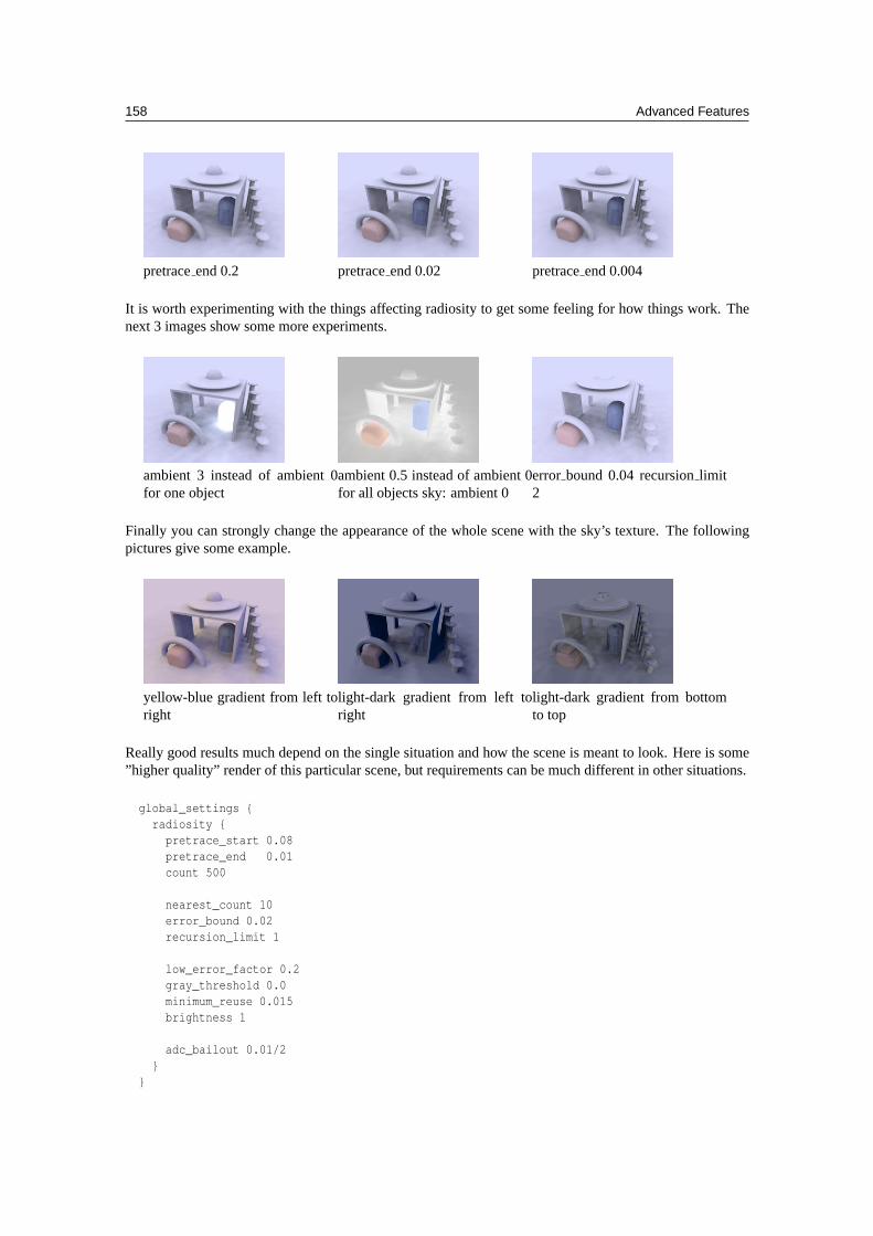
158 Advanced Features
pretraceend 0.2 pretraceend 0.02 pretraceend 0.004
It is worth experimenting with the things affecting radiosity to get some feeling for how things work. Thenext 3 images show some more experiments.
ambient 3 instead of ambient 0for one object
ambient 0.5 instead of ambient 0for all objects sky: ambient 0
error bound 0.04 recursionlimit2
Finally you can strongly change the appearance of the whole scene with the sky’s texture. The followingpictures give some example.
yellow-blue gradient from left toright
light-dark gradient from left toright
light-dark gradient from bottomto top
Really good results much depend on the single situation and how the scene is meant to look. Here is some”higher quality” render of this particular scene, but requirements can be much different in other situations.
global_settings {radiosity {
pretrace_start 0.08pretrace_end 0.01count 500
nearest_count 10error_bound 0.02recursion_limit 1
low_error_factor 0.2gray_threshold 0.0minimum_reuse 0.015brightness 1
adc_bailout 0.01/2}
}
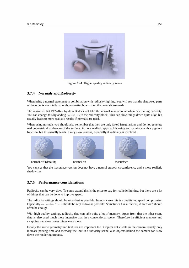
3.7 Radiosity 159
Figure 3.74: Higher quality radiosity scene
3.7.4 Normals and Radiosity
When using a normal statement in combination with radiosity lighting, you will see that the shadowed partsof the objects are totally smooth, no matter how strong the normals are made.
The reason is that POV-Ray by default does not take the normal into account when calculating radiosity.You can change this by addingnormal on to the radiosity block. This can slow things down quite a lot, butusually leads to more realistic results if normals are used.
When using normals you should also remember that they are only faked irregularities and do not generatereal geometric disturbances of the surface. A more realistic approach is using an isosurface with a pigmentfunction, but this usually leads to very slow renders, especially if radiosity is involved.
normal off (default) normal on isosurface
You can see that the isosurface version does not have a natural smooth circumference and a more realisticshadowline.
3.7.5 Performance considerations
Radiosity can be very slow. To some extend this is the price to pay for realistic lighting, but there are a lotof things that can be done to improve speed.
The radiosity settings should be set as fast as possible. In most cases this is a quality vs. speed compromise.Especiallyrecursion limit should be kept as low as possible. Sometimes1 is sufficient, if not2 or 3 shouldoften be enough.
With high quality settings, radiosity data can take quite a lot of memory. Apart from that the other scenedata is also used much more intensive than in a conventional scene. Therefore insufficient memory andswapping can slow down things even more.
Finally the scene geometry and textures are important too. Objects not visible in the camera usually onlyincrease parsing time and memory use, but in a radiosity scene, also objects behind the camera can slowdown the rendering process.
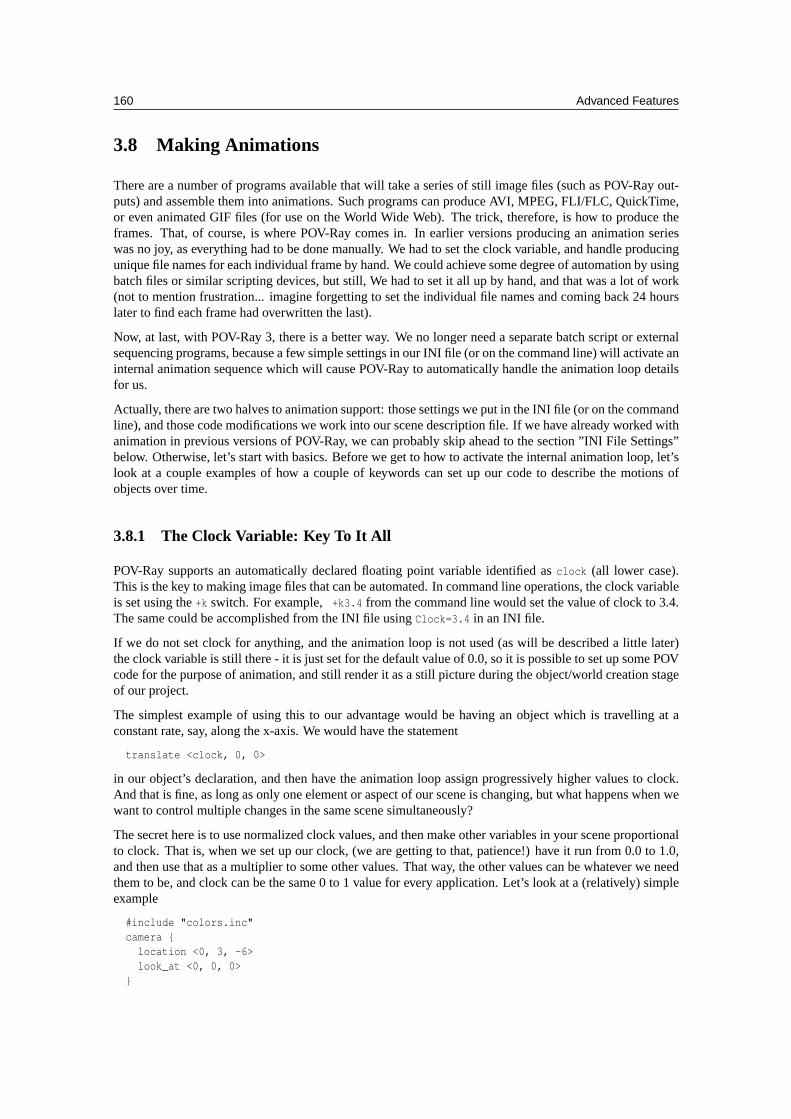
160 Advanced Features
3.8 Making Animations
There are a number of programs available that will take a series of still image files (such as POV-Ray out-puts) and assemble them into animations. Such programs can produce AVI, MPEG, FLI/FLC, QuickTime,or even animated GIF files (for use on the World Wide Web). The trick, therefore, is how to produce theframes. That, of course, is where POV-Ray comes in. In earlier versions producing an animation serieswas no joy, as everything had to be done manually. We had to set the clock variable, and handle producingunique file names for each individual frame by hand. We could achieve some degree of automation by usingbatch files or similar scripting devices, but still, We had to set it all up by hand, and that was a lot of work(not to mention frustration... imagine forgetting to set the individual file names and coming back 24 hourslater to find each frame had overwritten the last).
Now, at last, with POV-Ray 3, there is a better way. We no longer need a separate batch script or externalsequencing programs, because a few simple settings in our INI file (or on the command line) will activate aninternal animation sequence which will cause POV-Ray to automatically handle the animation loop detailsfor us.
Actually, there are two halves to animation support: those settings we put in the INI file (or on the commandline), and those code modifications we work into our scene description file. If we have already worked withanimation in previous versions of POV-Ray, we can probably skip ahead to the section ”INI File Settings”below. Otherwise, let’s start with basics. Before we get to how to activate the internal animation loop, let’slook at a couple examples of how a couple of keywords can set up our code to describe the motions ofobjects over time.
3.8.1 The Clock Variable: Key To It All
POV-Ray supports an automatically declared floating point variable identified asclock (all lower case).This is the key to making image files that can be automated. In command line operations, the clock variableis set using the+k switch. For example,+k3.4 from the command line would set the value of clock to 3.4.The same could be accomplished from the INI file usingClock=3.4 in an INI file.
If we do not set clock for anything, and the animation loop is not used (as will be described a little later)the clock variable is still there - it is just set for the default value of 0.0, so it is possible to set up some POVcode for the purpose of animation, and still render it as a still picture during the object/world creation stageof our project.
The simplest example of using this to our advantage would be having an object which is travelling at aconstant rate, say, along the x-axis. We would have the statement
translate <clock, 0, 0>
in our object’s declaration, and then have the animation loop assign progressively higher values to clock.And that is fine, as long as only one element or aspect of our scene is changing, but what happens when wewant to control multiple changes in the same scene simultaneously?
The secret here is to use normalized clock values, and then make other variables in your scene proportionalto clock. That is, when we set up our clock, (we are getting to that, patience!) have it run from 0.0 to 1.0,and then use that as a multiplier to some other values. That way, the other values can be whatever we needthem to be, and clock can be the same 0 to 1 value for every application. Let’s look at a (relatively) simpleexample
#include "colors.inc"camera {
location <0, 3, -6>look_at <0, 0, 0>
}
3.8 Making Animations 161
light_source { <20, 20, -20> color White }plane {
y, 0pigment { checker color White color Black }
}sphere {
<0, 0, 0> , 1pigment {
gradient xcolor_map {
[0.0 Blue ][0.5 Blue ][0.5 White ][1.0 White ]
}scale .25
}rotate <0, 0, -clock*360>translate <-pi, 1, 0>translate <2*pi*clock, 0, 0>
}
Assuming that a series of frames is run with the clock progressively going from 0.0 to 1.0, the above codewill produce a striped ball which rolls from left to right across the screen. We have two goals here:
1. Translate the ball from point A to point B, and,
2. Rotate the ball in exactly the right proportion to its linear movement to imply that it is rolling – notgliding – to its final position.
Taking the second goal first, we start with the sphere at the origin, because anywhere else and rotation willcause it to orbit the origin instead of rotating. Throughout the course of the animation, the ball will turnone complete 360 degree turn. Therefore, we used the formula,360*clock to determine the rotation in eachframe. Since clock runs 0 to 1, the rotation of the sphere runs from 0 degrees through 360.
Then we used the first translation to put the sphere at its initial starting point. Remember, we could not havejust declared it there, or it would have orbited the origin, so before we can meet our other goal (translation),we have to compensate by putting the sphere back where it would have been at the start. After that, were-translate the sphere by a clock relative distance, causing it to move relative to the starting point. Wehave chosen the formula of 2*pi* r*clock (the widest circumference of the sphere times current clockvalue) so that it will appear to move a distance equal to the circumference of the sphere in the same timethat it rotates a complete 360 degrees. In this way, we have synchronized the rotation of the sphere to itstranslation, making it appear to be smoothly rolling along the plane.
Besides allowing us to coordinate multiple aspects of change over time more cleanly, mathematically speak-ing, the other good reason for using normalized clock values is that it will not matter whether we are doinga ten frame animated GIF, or a three hundred frame AVI. Values of the clock are proportioned to the numberof frames, so that same POV code will work without regard to how long the frame sequence is. Our rollingball will still travel the exact same amount no matter how many frames our animation ends up with.
3.8.2 Clock Dependant Variables And Multi-Stage Animations
Okay, what if we wanted the ball to roll left to right for the first half of the animation, then change direction135 degrees and roll right to left, and toward the back of the scene. We would need to make use of POV-Ray’s new conditional rendering directives, and test the clock value to determine when we reach the halfwaypoint, then start rendering a different clock dependant sequence. But our goal, as above, it to be working ineach stage with a variable in the range of 0 to 1 (normalized) because this makes the math so much cleaner
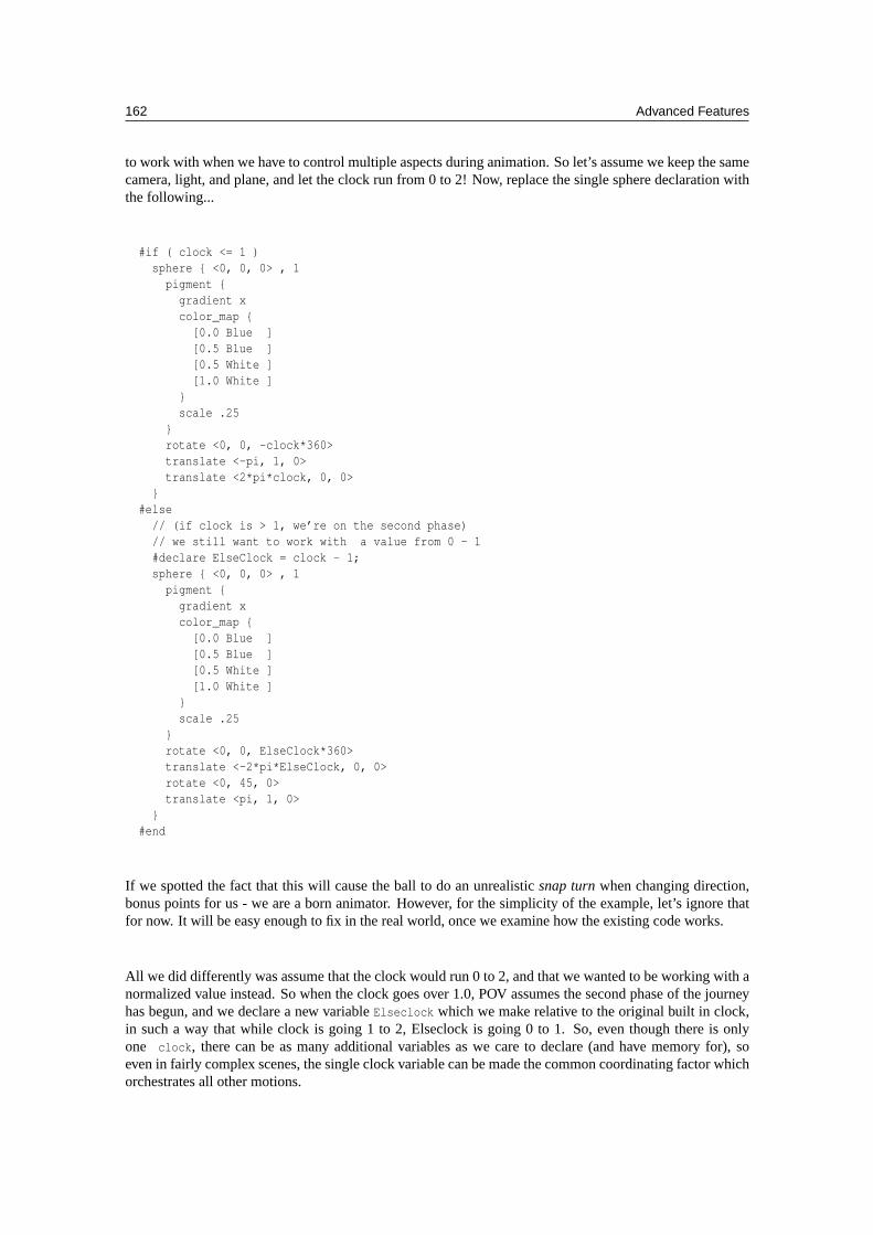
162 Advanced Features
to work with when we have to control multiple aspects during animation. So let’s assume we keep the samecamera, light, and plane, and let the clock run from 0 to 2! Now, replace the single sphere declaration withthe following...
#if ( clock <= 1 )sphere { <0, 0, 0> , 1
pigment {gradient xcolor_map {
[0.0 Blue ][0.5 Blue ][0.5 White ][1.0 White ]
}scale .25
}rotate <0, 0, -clock*360>translate <-pi, 1, 0>translate <2*pi*clock, 0, 0>
}#else
// (if clock is > 1, we’re on the second phase)// we still want to work with a value from 0 - 1#declare ElseClock = clock - 1;sphere { <0, 0, 0> , 1
pigment {gradient xcolor_map {
[0.0 Blue ][0.5 Blue ][0.5 White ][1.0 White ]
}scale .25
}rotate <0, 0, ElseClock*360>translate <-2*pi*ElseClock, 0, 0>rotate <0, 45, 0>translate <pi, 1, 0>
}#end
If we spotted the fact that this will cause the ball to do an unrealisticsnap turnwhen changing direction,bonus points for us - we are a born animator. However, for the simplicity of the example, let’s ignore thatfor now. It will be easy enough to fix in the real world, once we examine how the existing code works.
All we did differently was assume that the clock would run 0 to 2, and that we wanted to be working with anormalized value instead. So when the clock goes over 1.0, POV assumes the second phase of the journeyhas begun, and we declare a new variableElseclock which we make relative to the original built in clock,in such a way that while clock is going 1 to 2, Elseclock is going 0 to 1. So, even though there is onlyone clock, there can be as many additional variables as we care to declare (and have memory for), soeven in fairly complex scenes, the single clock variable can be made the common coordinating factor whichorchestrates all other motions.
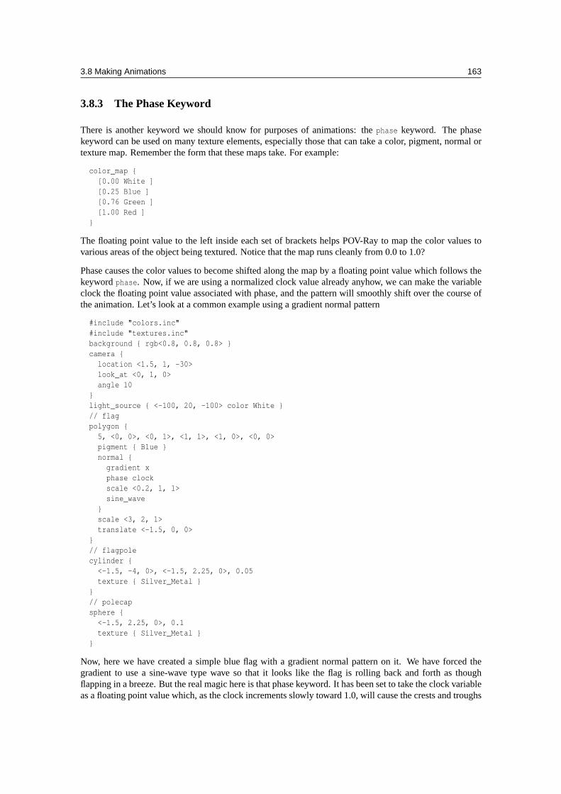
3.8 Making Animations 163
3.8.3 The Phase Keyword
There is another keyword we should know for purposes of animations: thephase keyword. The phasekeyword can be used on many texture elements, especially those that can take a color, pigment, normal ortexture map. Remember the form that these maps take. For example:
color_map {[0.00 White ][0.25 Blue ][0.76 Green ][1.00 Red ]
}
The floating point value to the left inside each set of brackets helps POV-Ray to map the color values tovarious areas of the object being textured. Notice that the map runs cleanly from 0.0 to 1.0?
Phase causes the color values to become shifted along the map by a floating point value which follows thekeywordphase. Now, if we are using a normalized clock value already anyhow, we can make the variableclock the floating point value associated with phase, and the pattern will smoothly shift over the course ofthe animation. Let’s look at a common example using a gradient normal pattern
#include "colors.inc"#include "textures.inc"background { rgb<0.8, 0.8, 0.8> }camera {
location <1.5, 1, -30>look_at <0, 1, 0>angle 10
}light_source { <-100, 20, -100> color White }// flagpolygon {
5, <0, 0>, <0, 1>, <1, 1>, <1, 0>, <0, 0>pigment { Blue }normal {
gradient xphase clockscale <0.2, 1, 1>sine_wave
}scale <3, 2, 1>translate <-1.5, 0, 0>
}// flagpolecylinder {
<-1.5, -4, 0>, <-1.5, 2.25, 0>, 0.05texture { Silver_Metal }
}// polecapsphere {
<-1.5, 2.25, 0>, 0.1texture { Silver_Metal }
}
Now, here we have created a simple blue flag with a gradient normal pattern on it. We have forced thegradient to use a sine-wave type wave so that it looks like the flag is rolling back and forth as thoughflapping in a breeze. But the real magic here is that phase keyword. It has been set to take the clock variableas a floating point value which, as the clock increments slowly toward 1.0, will cause the crests and troughs
164 Advanced Features
of the flag’s wave to shift along the x-axis. Effectively, when we animate the frames created by this code, itwill look like the flag is actually rippling in the wind.
This is only one, simple example of how a clock dependant phase shift can create interesting animationeffects. Trying phase will all sorts of texture patterns, and it is amazing the range of animation effects wecan create simply by phase alone, without ever actually moving the object.
3.8.4 Do Not Use Jitter Or Crand
One last piece of basic information to save frustration. Because jitter is an element of anti-aliasing, we couldjust as easily have mentioned this under the INI file settings section, but there are also forms of anti-aliasingused in area lights, and the new atmospheric effects of POV-Ray, so now is as good a time as any.
Jitter is a very small amount of random ray perturbation designed to diffuse tiny aliasing errors that mightnot otherwise totally disappear, even with intense anti-aliasing. By randomizing the placement of erroneouspixels, the error becomes less noticeable to the human eye, because the eye and mind are naturally inclinedto look for regular patterns rather than random distortions.
This concept, which works fantastically for still pictures, can become a nightmare in animations. Becauseit is random in nature, it will be different for each frame we render, and this becomes even more severe ifwe dither the final results down to, say 256 color animations (such as FLC’s). The result is jumping pixelsall over the scene, but especially concentrated any place where aliasing would normally be a problem (e.g.,where an infinite plane disappears into the distance).
For this reason, we should always set jitter tooff in area lights and anti-aliasing options when preparing ascene for an animation. The (relatively) small extra measure quality due to the use of jitter will be offset bythe ocean of jumpies that results. This general rule also applies to any truly random texture elements, suchascrand.
3.8.5 INI File Settings
Okay, so we have a grasp of how to code our file for animation. We know about the clock variable, userdeclared clock-relative variables, and the phase keyword. We know not to jitter or crand when we render ascene, and we are all set build some animations. Alright, let’s have at it.
The first concept we will need to know is the INI file settings,Initial Frame andFinal Frame. These arevery handy settings that will allow us to render a particular number of frames and each with its own uniqueframe number, in a completely hands free way. It is of course, so blindingly simple that it barely needsexplanation, but here is an example anyway. We just add the following lines to our favorite INI file settings
Initial_Frame = 1Final_Frame = 20
and we will initiate an automated loop that will generate 20 unique frames. The settings themselves willautomatically append a frame number onto the end of whatever we have set the output file name for, thusgiving each frame an unique file number without having to think about it. Secondly, by default, it willcycle the clock variable up from 0 to 1 in increments proportional to the number of frames. This is veryconvenient, since, no matter whether we are making a five frame animated GIF or a 300 frame MPEGsequence, we will have a clock value which smoothly cycles from exactly the same start to exactly the samefinish.
Next, about that clock. In our example with the rolling ball code, we saw that sometimes we want the clockto cycle through values other than the default of 0.0 to 1.0. Well, when that is the case, there are setting forthat too. The format is also quite simple. To make the clock run, as in our example, from 0.0 to 2.0, wewould just add to your INI file the linesInitial Clock = 0.0
3.9 While-loop tutorial 165
Final Clock = 2.0
Now, suppose we were developing a sequence of 100 frames, and we detected a visual glitch somewhere inframes, say 51 to 75. We go back over our code and we think we have fixed it. We would like to render justthose 25 frames instead of redoing the whole sequence from the beginning. What do we change?
If we said makeInitial Frame = 51, andFinal Frame = 75, we are wrong. Even though this would re-render files named with numbers 51 through 75, they will not properly fit into our sequence, because theclock will begin at its initial value starting with frame 51, and cycle to final value ending with frame 75.The only timeInitial Frame andFinal Frame should change is if we are doing an essentially new sequencethat will be appended onto existing material.
If we wanted to look at just 51 through 75 of the original animation, we need two new INI settingsSubset Start Frame = 51
Subset End Frame = 75
Added to settings from before, the clock will still cycle through its values proportioned from frames 1 to100, but we will only be rendering that part of the sequence from the 51st to the 75th frames.
This should give us a basic idea of how to use animation. Although, this introductory tutorial does not coverall the angles. For example, the last two settings we just saw, subset animation, can take fractional values,like 0.5 to 0.75, so that the number of actual frames will not change what portion of the animation is beingrendered. There is also support for efficient odd-even field rendering as would be useful for animationsprepared for display in interlaced playback such as television (see the reference section for full details).
With POV-Ray 3 now fully supporting a complete host of animation options, a whole fourth dimension isadded to the raytracing experience. Whether we are making a FLIC, AVI, MPEG, or simply an animatedGIF for our web site, animation support takes a lot of the tedium out of the process. And do not forgetthat phase and clock can be used to explore the range of numerous texture elements, as well as some of themore difficult to master objects (hint: the julia fractal for example). So even if we are completely contentwith making still scenes, adding animation to our repertoire can greatly enhance our understanding of whatPOV-Ray is capable of. Adventure awaits!
3.9 While-loop tutorial
Usually people who have never programmed have great difficulties understanding how simple while-loopswork and how they should be used. When you get into nested loops, the problem is even worse.
Sometimes even people who have programmed a bit with some language get confused with POV-Ray’swhile-loops. This usually happens when they have only used a for-loop which in itself has an index variable(which is often even incremented automatically).
3.9.1 What a while-loop is and what it is not
A while-loop in POV-Ray is just a control structure which tells POV-Ray to loop a command block whilethe specified condition is true (ie. until it gets false).
That is, a while-loop is like this:
#while(condition)...
#end
166 Advanced Features
The commands between#while and#end are run over and over as long as the condition evaluates to true.
A while-loop is not a for-loop nor any kind of loop which has an index variable by itself (which may beincremented automatically in each loop).
The while-loopdoes notcare what the conditions are between the parentheses (as long as they evaluate tosome value) or what does the block between#while and#end contain. It will just execute that block untilthe condition becomes false.
The while-loop does not do anything else. You can think about it as a kind of ”dumb” loop, which does notdo anything automatically (and this is not necessarily a bad thing).
3.9.2 How does a single while-loop work?
The while-loop works like this:
1. If the condition between the parentheses evaluates to false, jump to the command after the#end
statement. If the condition evaluates to true, just continue normally.
2. At the#end statement jump to the#while statement and start again.
That is:
• When POV-Ray gets to the#while statement it evaluates the condition between parentheses.
• If the statement evaluated to true then it will just continue normally with the next command.
• However, if the statement evaluated to false, POV-Ray will skip the entire body of the loop andcontinue from the command after the#end statement.
• At an #end statement POV-Ray will just jump back to the corresponding#while-statement and thencontinue normally (ie. testing the condition and so on).
Note that nowhere there is any mention about any index variable or anything else that could be used toautomatically end the loop or whatever. As said, it is just a ”dumb” loop that continues forever if necessary,only testing the statement between the parentheses (but it is not interested in what it is, only in its evaluatedvalue).
Although one could easily think that this kind of ”dumb” loop is bad and it should be more ”intelligent”and better, the fact is that this kind of ”dumb” loop is actually a lot more flexible and versatile. It allowsyou to make things not possible or very difficult to do with an ”intelligent” for-loop with automatic indexvariables.
3.9.3 How do I make a while-loop?
It depends on what you are trying to make.
The most common usage is to use it as a simple for-loop, that is, a loop which loops a certain number oftimes (for example 10 times) with an index value getting successive values (for example 1, 2, 3, ..., 10).
For this you need to first declare your index identifier with the first value. For example:
#declare Index = 1;
Now you want to loop 10 times. Remember how the condition worked: The while-loop loops as long as thecondition is true. So it should loop as long as our ’Index’ identifier is less or equal to 10:
#while(Index <= 10)
3.9 While-loop tutorial 167
When the ’Index’ gets the value 11 the loop ends, as it should.
Now we only have to add 1 to ’Index’ at each loop, so we should do it at the end of the loop, thus getting:
#declare Index = 1;#while(Index <= 10)
(some commands here)
#declare Index = Index + 1;#end
The incrementation before the#end is important. If we do not do it, ’Index’ would always have the value 1and the loop would go forever since 1 is always less or equal to 10.
What happens here?
1. First POV-Ray sets the value 1 to ’Index’.
2. Then it sees the#while statement and evaluates what is between the parentheses: Index<= 10
3. As ’Index’ has the value of 1 and 1<= 10, the condition evaluates to true.
4. So, it just continues normally. It executes the commands following the#while statement (denoted inthe above example as ”(some commands here)”).
5. Then it arrives normally to the last #declare command in the block. This causes the value 2 to beassigned to ’Index’.
6. Now it arrives the the#end command and so it just jumps to the#while.
7. After that it executes the steps 2-6 again because also 2 is less or equal to 10.
8. After this has been done 10 times, the value 11 is assigned to ’Index’ in the last command of theblock.
9. Now, when POV-Ray evaluates the condition it sees that it is false (because 11 is not less or equal to10). This causes POV-Ray to jump to the command after the#end statement.
10. The net effect of all this is that POV-Ray looped 10 times and the ’Index’ variable got successivevalues from 1 to 10 along the way.
If you read carefully the above description you will notice that the looping is done in a quite ”dumb” way,that is, there is no higher logic hidden inside the loop structure. In fact, POV-Ray does not have the slightestidea how many times the loop is executed and what variable is used to count the loops. It just follows orders.
The higher logic in this type of loop is in the combination of commands we wrote. The effect of thiscombination is that the loop works like a simple for-loop in most programming languages (like BASIC,etc).
3.9.4 What is a condition and how do I make one?
A condition is an expression that evaluates to a boolean value (ie. true or false) and is used in POV-Ray in#while-loops and#if-statements.
A condition is mainly a comparison between two values (although there are also some other ways of makinga condition, but that is not important now). For example:
1 < 2 is true1 > 2 is false1 = 1 is true1 = 2 is false
168 Advanced Features
and so on.
Usually it makes no sense to make comparisons like those. However, when comparing identifiers with somevalue or two identifiers together it starts to be very useful. Consider this:
#if(version < 3.1)#error "Wrong version!"
#end
If the identifier called ’version’ has a value which is less than 3.1 the#error line will be executed. If’version’ has a value which is 3.1 or greater, the#error line is just skipped.
You can combine conditions together with the boolean operators & (and) and — (or). You can also invertthe value of a condition with ! (not).
For example, if you want something to be done when ’a’ is less than 10and ’b’ is greater or equal to 20,the condition would be:
a<10 \& b>=20
For more information about these comparison operators, see the ’Float operators’ section of the POV-Raydocumentation.
3.9.5 What about loop types other than simple for-loops?
As POV-Ray does not care what the condition is and what we are using to make that condition, we can usethe while-loop in many other ways.
For example, this is a typical use of the while-loop which is not a simple for-loop:
#declare S = seed(0);#declare Point = <2*rand(S)-1, 2*rand(S)-1, 2*rand(S)-1>;#while(vlength(Point) > 1)
#declare Point = <2*rand(S)-1, 2*rand(S)-1, 2*rand(S)-1>;#end
What we are doing here is this: Take a random point between<-1, -1, -1> and<1, 1, 1> and if it is notinside the unit sphere take another random point in that range. Do this until we get a point inside the unitsphere.
This is not an unrealistic example since it is very handy.
As we see, this has nothing to do with an ordinary for-loop:
• It does not have any ”index” value which gets consecutive values during the loop.
• We do not know how many times it will loop. In this case it loops a random number of times.
• For-loops are usually used to get a series of things (eg. objects). At each loop another instance of thatthing is created. Here, however, we are only interested in the value that resultsafter the loop, not thevalues inside it.
As we can see, a while-loop can also be used for a task of type ”calculate a value or some values until theresult is inside a specified range” (among many other tasks).
By the way, there is a variant of this kind of loop where the task is: ”Calculate a value until the result isinside a specified range, but make only a certain number of tries. If the value does not get inside that rangeafter that number of tries, stop trying”. This is used when there is a possibility for the loop for going onforever.
3.9 While-loop tutorial 169
In the above example about the point inside the unit sphere we do not need this because the random pointwill surely hit the inside of the sphere at some time. In some other situations, however, we cannot be sosure.
In this case we need a regular index variable to count the number of loops. If we have made that amount ofloops then we stop.
Suppose that we wanted to modify our point searching program to be completely safe and to try only up to10 times. If the point does not hit the inside of the sphere after 10 tries, we just give up and take the point<0,0,0>.
#declare S = seed(0);#declare Point = <2*rand(S)-1, 2*rand(S)-1, 2*rand(S)-1>;#declare Index = 1;#while(Index <= 10 \& vlength(Point) > 1)
#declare Point = <2*rand(S)-1, 2*rand(S)-1, 2*rand(S)-1>;#declare Index = Index + 1;
#end
#if(vlength(Point) > 1)#declare Point = <0,0,0>
#end
What did we do?
• We added an ’Index’ value which counts the amount of loops gone so far. It is quite similar to theindex loop of a simple for-loop.
• We added an extra condition to the while-loop: Besides testing that the point is outside the unit sphereit also tests that our index variable has not bailed out. So now there are two conditions for the loopto continue: The ’Index’ value must be less or equal to 10and the ’Point’ has to be outside the unitsphere. If either one of them fails, the loop is ended.
• Then we check if the point is still outside the unit sphere. If it is, we just take<0,0,0>.
Btw, sometimes it is not convenient to make the test again in the#if statement. There is another way ofdetermining whether the loop bailed out without successful termination or not: Since the loop ends whenthe ’Index’ gets the value 11, we can use this to test the successfulness of the loop:
#if(Index = 11)(loop was not successful)
#end
3.9.6 What about nested loops?
Even when one masters simple loops, nested loops can be a frightening thing (or at least hard to understand).
Nested loops are used for example for creating a 2D array of objects (with rows and columns of objects),etc. For example if you want to create a 10x20 array of spheres in your scene, a nested loop is the tool forit.
There is nothing special about nested loops. You only have to pay attention to where you initialize andupdate your index variables.
Let’s recall the form of a simple for-loop:
#declare Index = initial_value;#while(Index <= final_value)
[Something here]
170 Advanced Features
#declare Index = Index + index_step;#end
The [Something here] part can be anything. If it is another while-loop, then we have nested loops. Theinner loop should have the same structure as the outer one.
Note that proper indentation helps us distinguishing between the loops. It is always a good idea to use agood indentation scheme:
#declare Index1 = initial_value1;#while(Index1 <= final_value1)
#declare Index2 = initial_value2;#while(Index2 <= final_value2)
[Something here]
#declare Index2 = Index2 + index2_step;#end
#declare Index1 = Index1 + index1_step;#end
It is a common mistake for beginners to break this structure. For example it is common to declare the’Index2’ before the first#while. This breaks the for-loop structure and thus does not work. If you followstep by step what POV-Ray does, as explained earlier, you will see why it does not work. Do not mix thestructures of the inner and the outer loops together or your code will simply not work as expected.
So, if we want to make our 10x20 array of spheres, it will look like this:
#declare Index1 = 0;#while(Index1 <= 9)
#declare Index2 = 0;#while(Index2 <= 19)
sphere { <Index1, Index2, 0>, .5 }
#declare Index2 = Index2 + 1;#end
#declare Index1 = Index1 + 1;#end
Note how we now start from 0 and continue to 9 in the outer loop and from 0 to 19 in the inner loop. Thishas been done to get the sphere array start from the origin (instead of starting from<1, 1, 0>). Of coursewe could have made the ’Index1’ and ’Index2’ go from 1 to 10 and from 1 to 20 respectively and thencreated the sphere in this way:
sphere { <Index1-1, Index2-1, 0>, .5 }
Although you should not mix the loop structures together, you can perfectly use the values of the outer loopin the inner loop (eg. in its condition). For example, if we wanted to create a triangular array of spheresinstead of a rectangular one (that is, we create only half of the spheres), we could have made the inner#while like this:
#while(Index2 < Index1*2)
(’Index2’ will go from 0 to the value of ’Index1’ multiplied by 2.)
3.9 While-loop tutorial 171
There is no reason why we should limit ourselves to just two nested loops. There is virtually no limit howmany loops you can nest. For example, if we wanted to create a box-shape filled by spheres rows, columsand depth, we just make three nested loops, one for the x-axis, another for the y-axis and the third for thez-axis.
3.9.7 Mixed-type nested loops
It is perfectly possible to put a for-loop inside a non-for-loop or vice-versa. Again, you just have to becareful (with experience it gets easier).
For example, suppose that we want to create 50 spheres which are randomly placed inside the unit sphere.
So the distinction is clear: First we need a loop to create 50 spheres (a for-loop type suffices) and then weneed another loop inside it to calculate the location of the sphere. It will look like this:
#declare S = seed(0);#declare Index = 1;#while(Index <= 50)
#declare Point = <2*rand(S)-1, 2*rand(S)-1, 2*rand(S)-1>;#while(vlength(Point) > 1)
#declare Point = <2*rand(S)-1, 2*rand(S)-1, 2*rand(S)-1>;#end
sphere { Point, .1 }
#declare Index = Index + 1;#end
There are some important things to note in this specific example:
• Although this is a nested loop, the sphere is not created in the inner loop but in the outer one. Thereason is clear: We want to create 50 spheres, so the sphere creation has to be inside the loop thatcounts to 50. The inner loop just calculates an appropriate location.
• The seed value ’S’ is declared outside all the loops although it is used only in the inner loop. Can youguess why? (Putting it inside the outer loop would have caused an undesired result: Which one?)
3.9.8 Other things to note
There is no reason why the index value in your simple for-loop should step one unit at a time. Since thewhile-loop does not care how the index changes, you can change it in whichever way you want. Eg:
#declare Index = Index - 1; Decrements the index (be careful with thewhile loop condition)
#declare Index = Index + 0.2; Increases by steps of 0.2
#declare Index = Index * 2; Doubles the value of the index at each step.
etc.
- Be carefulwhereyou put your while-loop.
I have seen this kind of mistake more than once:
#declare Index = 1;#while(Index <= 10)
172 Advanced Features
blob{ threshold 0.6
sphere { <Index, 0, 0>, 2, 1 }}#declare Index = Index + 1;
#end
You will probably see immediately the problem.
This code creates 10 blobs with one component each. It does not seem to make much sense. Most probablythe user wanted to make one blob with 10 components.
Why did this mistake happen? It may be that the user (more or less subconsciously) thought that the while-loop must be the outermost control structure and does not realize that while-loops can be anywhere, alsoinside objects (creating subcomponents or whatever).
The correct code is, of course:
blob{ threshold 0.6
#declare Index = 1;#while(Index <= 10)
sphere { <Index, 0, 0>, 2, 1 }
#declare Index = Index + 1;#end
}
The essential difference here is that it is only the sphere code which is run 10 times instead of the wholeblob code. The net result is the same as if we had written the sphere code 10 times with proper values of’Index’.
Be also careful with the placement of the braces. If you put them in the wrong place you can end upaccidentally repeating an opening or a closing brace 10 times. Again, a proper indentation usually helps alot with this (as seen in the above example).
- Tip: You can use while-loops in conjunction with arrays to automatize the creation of long lists of elementswith differing data.
Imagine that you are making something like this:
color_map{ [0.00 rgb <.1,1,.6>]
[0.05 rgb <.8,.3,.6>][0.10 rgb <.3,.7,.9>][0.15 rgb <1,.7,.3>]...and so on
It is tedious to have to write the same things over and over just changing the index value and the values inthe vector (even if you use copy-paste to copy the lines).
There is also one very big problem here: If you ever want to add a new color to the color map or remove acolor, you would have to renumber all the indices again, which can be extremely tedious and frustrating.
Would not it be nice to automatize the creation of the color map so that you only have to write the vectorsand that is it?
Well, you can. Using a while-loop which reads an array of vectors:
3.10 SDL tutorial: A raytracer 173
#declare MyColors = array[20]{ <.1,1,.6>, <.8,.3,.6>, <.3,.7,.9>,
<1,.7,.3>, ...}
...
color_map{ #declare LastIndex = dimension_size(MyColors, 1)-1;
#declare Index = 0;#while(Index <= LastIndex)
[Index/LastIndex rgb MyColors[Index]]
#declare Index = Index + 1;#end
}
Now it is easy to add, remove or modify colors in your color map. Just edit the vector array (rememberingto change its size number accordingly) and the while-loop will automatically calculate the right values andcreate the color map for you.
3.10 SDL tutorial: A raytracer
You know you have been raytracing too long when ...... You’ve been asked how you did that thing you did, by the author of the raytracer you used to do it.
– Alex McLeod
3.10.1 Introduction
A raytracer made with POV-Ray sounds really weird, doesn’t it? What is it anyways? POV-Ray is alreadya raytracer in itself, how can we use it to make a raytracer? What the...?
The idea is to make a simple sphere raytracer which supports colored spheres (with diffuse and specularlighting), colored light sources, reflections and shadows with the POV-Ray SDL (Scene Description Lan-guage), then just render the image created this way. That is, we do not use POV-Ray itself to raytrace thespheres, but we make our own raytracer with its SDL and use POV-Ray’s raytracing part to just get theimage on screen.
What obscure idea could be behind this weirdness (besides a very serious case of YHBRFTLW...)? Why donot just use POV-Ray itself to raytrace the spheres a lot faster and that is it?
The idea is not speed nor quality, but to show the power of the POV-Ray SDL. If you know how to makesuch a thing as a raytracer with it, we can really grasp the expressive power of the SDL.
The idea of this document is to make a different approach to POV-Ray SDL teaching. It is intended to be adifferent type of tutorial: Instead of starting from the basics and give simple and dumb examples, we jumpright into a high-end SDL code and see how it is done. However, this is done in a way that even beginnerscan learn something from it.
Another advantage is that you will learn how a simple sphere raytracer is done by reading this tutorial.There are lots of misconceptions about raytracing out there, and knowing how to make one helps clear mostof them.
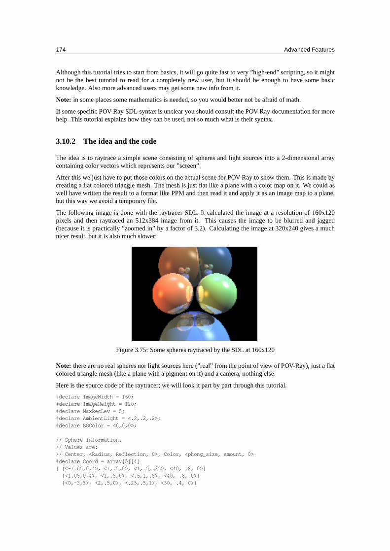
174 Advanced Features
Although this tutorial tries to start from basics, it will go quite fast to very ”high-end” scripting, so it mightnot be the best tutorial to read for a completely new user, but it should be enough to have some basicknowledge. Also more advanced users may get some new info from it.
Note: in some places some mathematics is needed, so you would better not be afraid of math.
If some specific POV-Ray SDL syntax is unclear you should consult the POV-Ray documentation for morehelp. This tutorial explains how they can be used, not so much what is their syntax.
3.10.2 The idea and the code
The idea is to raytrace a simple scene consisting of spheres and light sources into a 2-dimensional arraycontaining color vectors which represents our ”screen”.
After this we just have to put those colors on the actual scene for POV-Ray to show them. This is made bycreating a flat colored triangle mesh. The mesh is just flat like a plane with a color map on it. We could aswell have written the result to a format like PPM and then read it and apply it as an image map to a plane,but this way we avoid a temporary file.
The following image is done with the raytracer SDL. It calculated the image at a resolution of 160x120pixels and then raytraced an 512x384 image from it. This causes the image to be blurred and jagged(because it is practically ”zoomed in” by a factor of 3.2). Calculating the image at 320x240 gives a muchnicer result, but it is also much slower:
Figure 3.75: Some spheres raytraced by the SDL at 160x120
Note: there are no real spheres nor light sources here (”real” from the point of view of POV-Ray), just a flatcolored triangle mesh (like a plane with a pigment on it) and a camera, nothing else.
Here is the source code of the raytracer; we will look it part by part through this tutorial.
#declare ImageWidth = 160;#declare ImageHeight = 120;#declare MaxRecLev = 5;#declare AmbientLight = <.2,.2,.2>;#declare BGColor = <0,0,0>;
// Sphere information.// Values are:// Center, <Radius, Reflection, 0>, Color, <phong_size, amount, 0>#declare Coord = array[5][4]{ {<-1.05,0,4>, <1,.5,0>, <1,.5,.25>, <40, .8, 0>}
{<1.05,0,4>, <1,.5,0>, <.5,1,.5>, <40, .8, 0>}{<0,-3,5>, <2,.5,0>, <.25,.5,1>, <30, .4, 0>}
3.10 SDL tutorial: A raytracer 175
{<-1,2.3,9>, <2,.5,0>, <.5,.3,.1>, <30, .4, 0>}{<1.3,2.6,9>, <1.8,.5,0>, <.1,.3,.5>, <30, .4, 0>}
}
// Light source directions and colors:#declare LVect = array[3][2]{ {<-1, 0, -.5>, <.8,.4,.1>}
{<1, 1, -.5>, <1,1,1>}{<0,1,0>, <.1,.2,.5>}
}
//==================================================================// Raytracing calculations://==================================================================#declare MaxDist = 1e5;#declare ObjAmnt = dimension_size(Coord, 1);#declare LightAmnt = dimension_size(LVect, 1);
#declare Ind = 0;#while(Ind < LightAmnt)
#declare LVect[Ind][0] = vnormalize(LVect[Ind][0]);#declare Ind = Ind+1;
#end
#macro calcRaySphereIntersection(P, D, sphereInd)#local V = P-Coord[sphereInd][0];#local R = Coord[sphereInd][1].x;
#local DV = vdot(D, V);#local D2 = vdot(D, D);#local SQ = DV*DV-D2*(vdot(V, V)-R*R);#if(SQ < 0) #local Result = -1;#else
#local SQ = sqrt(SQ);#local T1 = (-DV+SQ)/D2;#local T2 = (-DV-SQ)/D2;#local Result = (T1<T2 ? T1 : T2);
#endResult
#end
#macro Trace(P, D, recLev)#local minT = MaxDist;#local closest = ObjAmnt;
// Find closest intersection:#local Ind = 0;#while(Ind < ObjAmnt)
#local T = calcRaySphereIntersection(P, D, Ind);#if(T>0 \& T<minT)
#local minT = T;#local closest = Ind;
#end#local Ind = Ind+1;
#end
176 Advanced Features
// If not found, return background color:#if(closest = ObjAmnt)
#local Pixel = BGColor;#else
// Else calculate the color of the intersection point:#local IP = P+minT*D;#local R = Coord[closest][1].x;#local Normal = (IP-Coord[closest][0])/R;
#local V = P-IP;#local Refl = 2*Normal*(vdot(Normal, V)) - V;
// Lighting:#local Pixel = AmbientLight;#local Ind = 0;#while(Ind < LightAmnt)
#local L = LVect[Ind][0];
// Shadowtest:#local Shadowed = false;#local Ind2 = 0;#while(Ind2 < ObjAmnt)
#if(Ind2!=closest \& calcRaySphereIntersection(IP,L,Ind2)>0)#local Shadowed = true;#local Ind2 = ObjAmnt;
#end#local Ind2 = Ind2+1;
#end
#if(!Shadowed)// Diffuse:#local Factor = vdot(Normal, L);#if(Factor > 0)
#local Pixel=Pixel+LVect[Ind][1]*Coord[closest][2]*Factor;#end
// Specular:#local Factor = vdot(vnormalize(Refl), L);#if(Factor > 0)
#local Pixel =Pixel +LVect[Ind][1]*pow(Factor, Coord[closest][3].x)*Coord[closest][3].y;
#end#end#local Ind = Ind+1;
#end
// Reflection:#if(recLev < MaxRecLev \& Coord[closest][1].y > 0)
#local Pixel =Pixel + Trace(IP, Refl, recLev+1)*Coord[closest][1].y;#end
#end
Pixel#end
3.10 SDL tutorial: A raytracer 177
#debug "Rendering...\n\n"#declare Image = array[ImageWidth][ImageHeight]#declare IndY = 0;#while(IndY < ImageHeight)
#declare CoordY = IndY/(ImageHeight-1)*2-1;#declare IndX = 0;#while(IndX < ImageWidth)
#declare CoordX =(IndX/(ImageWidth-1)-.5)*2*ImageWidth/ImageHeight;
#declare Image[IndX][IndY] =Trace(-z*3, <CoordX, CoordY, 3>, 1);
#declare IndX = IndX+1;#end#declare IndY = IndY+1;#debug concat("\rDone ", str(100*IndY/ImageHeight, 0, 1),
"\% (line ",str(IndY,0,0)," out of ",str(ImageHeight,0,0),")")#end#debug "\n"
//==================================================================// Image creation (colored mesh)://==================================================================#default { finish { ambient 1 } }
#debug "Creating colored mesh to show image...\n"mesh2{ vertex_vectors
{ ImageWidth*ImageHeight*2,#declare IndY = 0;#while(IndY < ImageHeight)
#declare IndX = 0;#while(IndX < ImageWidth)
<(IndX/(ImageWidth-1)-.5)*ImageWidth/ImageHeight*2,IndY/(ImageHeight-1)*2-1, 0>,
<((IndX+.5)/(ImageWidth-1)-.5)*ImageWidth/ImageHeight*2,(IndY+.5)/(ImageHeight-1)*2-1, 0>
#declare IndX = IndX+1;#end#declare IndY = IndY+1;
#end}texture_list{ ImageWidth*ImageHeight*2,
#declare IndY = 0;#while(IndY < ImageHeight)
#declare IndX = 0;#while(IndX < ImageWidth)
texture { pigment { rgb Image[IndX][IndY] } }#if(IndX < ImageWidth-1 \& IndY < ImageHeight-1)
texture { pigment { rgb(Image[IndX][IndY]+Image[IndX+1][IndY]+Image[IndX][IndY+1]+Image[IndX+1][IndY+1])/4 } }
#elsetexture { pigment { rgb 0 } }
#end#declare IndX = IndX+1;
178 Advanced Features
#end#declare IndY = IndY+1;
#end}face_indices{ (ImageWidth-1)*(ImageHeight-1)*4,
#declare IndY = 0;#while(IndY < ImageHeight-1)
#declare IndX = 0;#while(IndX < ImageWidth-1)
<IndX*2+ IndY *(ImageWidth*2),IndX*2+2+IndY *(ImageWidth*2),IndX*2+1+IndY *(ImageWidth*2)>,IndX*2+ IndY *(ImageWidth*2),IndX*2+2+IndY *(ImageWidth*2),IndX*2+1+IndY *(ImageWidth*2),
<IndX*2+ IndY *(ImageWidth*2),IndX*2+ (IndY+1)*(ImageWidth*2),IndX*2+1+IndY *(ImageWidth*2)>,IndX*2+ IndY *(ImageWidth*2),IndX*2+ (IndY+1)*(ImageWidth*2),IndX*2+1+IndY *(ImageWidth*2),
<IndX*2+ (IndY+1)*(ImageWidth*2),IndX*2+2+(IndY+1)*(ImageWidth*2),IndX*2+1+IndY *(ImageWidth*2)>,IndX*2+ (IndY+1)*(ImageWidth*2),IndX*2+2+(IndY+1)*(ImageWidth*2),IndX*2+1+IndY *(ImageWidth*2),
<IndX*2+2+IndY *(ImageWidth*2),IndX*2+2+(IndY+1)*(ImageWidth*2),IndX*2+1+IndY *(ImageWidth*2)>,IndX*2+2+IndY *(ImageWidth*2),IndX*2+2+(IndY+1)*(ImageWidth*2),IndX*2+1+IndY *(ImageWidth*2)
#declare IndX = IndX+1;#end#declare IndY = IndY+1;
#end}
}
camera { orthographic location -z*2 look_at 0 }
3.10.3 Short introduction to raytracing
Before we start looking at the code, let’s look briefly how raytracing works. This will help you understandwhat the script is doing.
The basic idea of raytracing is to ”shoot” rays from the camera towards the scene and see what does the rayhit. If the ray hits the surface of an object then lighting calculations are performed in order to get the colorof the surface at that place.
The following image shows this graphically:
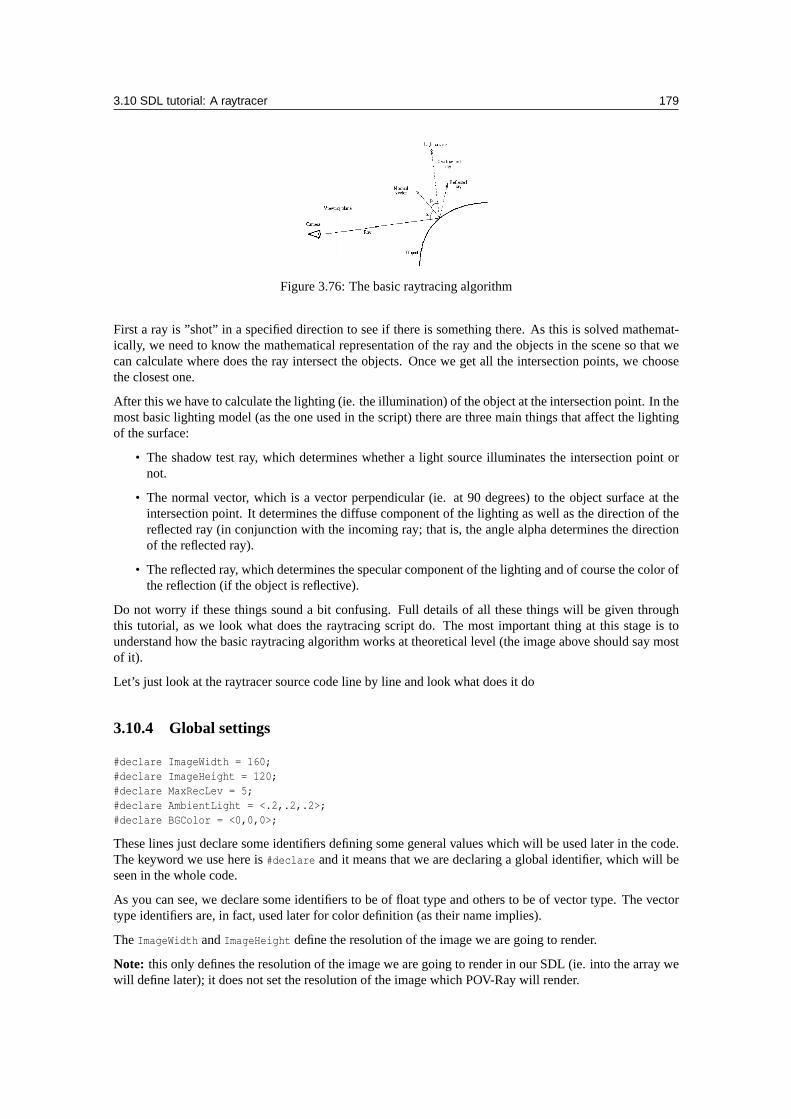
3.10 SDL tutorial: A raytracer 179
Figure 3.76: The basic raytracing algorithm
First a ray is ”shot” in a specified direction to see if there is something there. As this is solved mathemat-ically, we need to know the mathematical representation of the ray and the objects in the scene so that wecan calculate where does the ray intersect the objects. Once we get all the intersection points, we choosethe closest one.
After this we have to calculate the lighting (ie. the illumination) of the object at the intersection point. In themost basic lighting model (as the one used in the script) there are three main things that affect the lightingof the surface:
• The shadow test ray, which determines whether a light source illuminates the intersection point ornot.
• The normal vector, which is a vector perpendicular (ie. at 90 degrees) to the object surface at theintersection point. It determines the diffuse component of the lighting as well as the direction of thereflected ray (in conjunction with the incoming ray; that is, the angle alpha determines the directionof the reflected ray).
• The reflected ray, which determines the specular component of the lighting and of course the color ofthe reflection (if the object is reflective).
Do not worry if these things sound a bit confusing. Full details of all these things will be given throughthis tutorial, as we look what does the raytracing script do. The most important thing at this stage is tounderstand how the basic raytracing algorithm works at theoretical level (the image above should say mostof it).
Let’s just look at the raytracer source code line by line and look what does it do
3.10.4 Global settings
#declare ImageWidth = 160;#declare ImageHeight = 120;#declare MaxRecLev = 5;#declare AmbientLight = <.2,.2,.2>;#declare BGColor = <0,0,0>;
These lines just declare some identifiers defining some general values which will be used later in the code.The keyword we use here is#declare and it means that we are declaring a global identifier, which will beseen in the whole code.
As you can see, we declare some identifiers to be of float type and others to be of vector type. The vectortype identifiers are, in fact, used later for color definition (as their name implies).
TheImageWidth andImageHeight define the resolution of the image we are going to render.
Note: this only defines the resolution of the image we are going to render in our SDL (ie. into the array wewill define later); it does not set the resolution of the image which POV-Ray will render.
180 Advanced Features
TheMaxRecLev limits the maximum number of recursive reflections the code will calculate. It is equivalentto themax trace level value inglobal settings which POV-Ray uses to raytrace.
The AmbientLight defines a color which is added to all surfaces. This is used to ”lighten up” shadowedparts so that they are not completely dark. It is equivalent to theambient light value inglobal settings.
Finally, BGColor defines the color of the rays which do not hit anything. It is equivalent to thebackground
block of POV-Ray.
3.10.5 Scene definition
// Sphere information.// Values are:// Center, <Radius, Reflection, 0>, Color, <phong_size, amount, 0>#declare Coord = array[5][4]{ {<-1.05,0,4>, <1,.5,0>, <1,.5,.25>, <40, .8, 0>}
{<1.05,0,4>, <1,.5,0>, <.5,1,.5>, <40, .8, 0>}{<0,-3,5>, <2,.5,0>, <.25,.5,1>, <30, .4, 0>}{<-1,2.3,9>, <2,.5,0>, <.5,.3,.1>, <30, .4, 0>}{<1.3,2.6,9>, <1.8,.5,0>, <.1,.3,.5>, <30, .4, 0>}
}
// Light source directions and colors:#declare LVect = array[3][2]{ {<-1, 0, -.5>, <.8,.4,.1>}
{<1, 1, -.5>, <1,1,1>}{<0,1,0>, <.1,.2,.5>}
}
Here we use a bit more complex declarations: Array declarations.
In fact, they are even more complex than simple arrays, as we are declaring two-dimensional arrays.
A simple one-dimensional array can be declared like:
#declare MyArray = array[4] { 1, 2, 3, 4 }
and then values can be read from inside it with for example:MyArray[2] (which will return3 in this case asthe indexing starts from 0, ie. the index 0 gets the first value in the array).
A two-dimensional array can be thought as an array containing arrays. That is, if you sayarray[3][2], thatmeans ”an array which has 3 elements; each one of those elements is an array with 2 elements”. When youwant to read a value from it, for exampleMyArray[1][3], you can think about it as ”get the fourth valuefrom the second array” (as indexing starts from 0, then the index value 3 actually means ”fourth value”).
Note: although you can put almost anything inside an array (floats, vectors, objects and so on) you canonly put one type of things inside an array. That is, you cannot mix float values and objects inside the samearray. (One nice feature is that all POV-Ray objects are considered equivalent, which means that an objectarray can contain any objects inside it.)
What we are doing here is to define the information for our spheres and light sources. The first array (calledCoord) defines the information for the spheres and the second (LVect) defines the light sources.
For spheres we define their center as the first vector. The second vector has both the radius of the sphereand its reflection amount (which is equivalent to thereflection value in thefinish block of an object).This is a trick we use to not to waste so much space, so we use two values of the same vector for definingtwo different things.
The third vector defines the color of the sphere and the fourth the specular component of the lighting(equivalent tophong size andphong values in thefinish block of an object).
3.10 SDL tutorial: A raytracer 181
The light source definition array contains direction vectors and colors. This means that the light sources aredirectional, that is, they just say which direction the light is coming from. It could have been equally easyto make point lights, though.
We will use the information inside these arrays later in order to raytrace the scene they define.
3.10.6 Initializing the raytracer
#declare MaxDist = 1e5;#declare ObjAmnt = dimension_size(Coord, 1);#declare LightAmnt = dimension_size(LVect, 1);
#declare Ind = 0;#while(Ind < LightAmnt)
#declare LVect[Ind][0] = vnormalize(LVect[Ind][0]);#declare Ind = Ind+1;
#end
Before being able to start the raytracing, we have to intialize a couple of things.
TheMaxDist defines the maximum distance a surface can be from the starting point of a ray. This meansthat if a surface is farther away from the starting point of the ray than this value, it will not be seen. Strictlyspeaking this value is unnecessary and we can make the raytracer so that there is no such a limitation, butwe save one extra step when we do it this way, and for scenes sized like ours it does not really matter. (Ifyou really, really want to get rid of the limitation, I am sure you will figure out yourself how to do it afterthis tutorial.)
TheObjAmnt andLightAmnt identifiers are declared just to make it easier for us to see how many objects andlights are there (we need this info to loop through all the objects and lights). Calling thedimension size()
function is a really nice way of getting the number of items in an array.
All right, now we are getting to a bit more advanced stuff: What does the while-loop do there?
The#while-loop uses theInd identifier as an index value going from0 to LightAmnt-1 (yes,-1; whenIndgets the valueLightAmnt the loop is ended right away). We also see that we are indexing theLVect array;thus, it is clear we are going through all the light sources (specifically through their direction vectors, as weonly use the[0] part) and we assign something to them.
What we are doing is to assign a normalized version of each light source direction onto themselves, that is,just normalizing them.
Normalize is a synonym for ”convert to unit vector”, that is, convert to a vector with the same direction asthe original but with length 1.
Why? We will later see that for illumination calculations we will be needing unit vectors. It is more efficientto convert the light source directions to unit vectors once at the beginning than every time for each pixellater.
3.10.7 Ray-sphere intersection
#macro calcRaySphereIntersection(P, D, sphereInd)#local V = P-Coord[sphereInd][0];#local R = Coord[sphereInd][1].x;
#local DV = vdot(D, V);#local D2 = vdot(D, D);#local SQ = DV*DV-D2*(vdot(V, V)-R*R);
182 Advanced Features
#if(SQ < 0) #local Result = -1;#else
#local SQ = sqrt(SQ);#local T1 = (-DV+SQ)/D2;#local T2 = (-DV-SQ)/D2;#local Result = (T1<T2 ? T1 : T2);
#endResult
#end
This is the core of the whole raytracing process.
First let’s see how a macro works (if you know it, just skip the following section):
Inner workings of a #macro
A macro works like a substitution command (similar to the #define macros in the C programming language).The body of the macro is in practice inserted in the place where the macro is called. For example you canuse a macro like this:
#macro UnitSphere()sphere { 0,1 }
#end
object { UnitSphere() pigment { rgb 1 } }
The result of this code is, in effect, as if you had written:
object { sphere { 0,1 } pigment { rgb 1 } }
Of course there is no reason in making this, as you could have just #declared theUnitSphere as a sphere ofradius 1. However, the power of macros kick in when you start using macro parameters. For example:
#macro Sphere(Radius)sphere { 0, Radius }
#end
object { Sphere(3) pigment { rgb 1 } }
Now you can use the macroSphere to create a sphere with the specified radius. Of course this does notmake much sense either, as you could just write the sphere primitive directly because it is so short, butthis example is intentionally short to show how it works; the macros become very handy when they createsomething much more complicated than just a sphere.
There is one important difference between macros in POV-Ray and real substitution macros: Any#local
statement inside the macro definition will be parsed at the visibility level of the macro only, that is, it willhave no effect on the environment where the macro was called from. The following example shows what Iam talking about:
#macro Sphere(Radius)#local Color = <1,1,1>;sphere { 0, Radius pigment { rgb Color } }
#end
#declare Color = <1,0,0>;object { Sphere(3) }
// ’Color’ is still <1,0,0> here,// thus the following box will be red:
box { -1,1 pigment { rgb Color } }
3.10 SDL tutorial: A raytracer 183
In the example above, although the macro creates a local identifier calledColor and there is an identifierwith the same name at global level, the local definition does not affect the global one. Also even if therewas not any global definition ofColor, the one inside the macro is not seen outside it.
There is one important exception to this, and this is one of the most powerful features of macros (thanks tothis they can be used as if they were functions): If an identifier (be it local or global) appears alone in thebody of a macro (usually at the end), its value will be passed outside the macro (as if it was a return value).The following example shows how this works:
#macro Factorial(N)#local Result = 1;#local Ind = 2;#while(Ind <= N)
#local Result = Result*Ind;#local Ind = Ind+1;
#endResult
#end
#declare Value = Factorial(5);
Although the identifierResult is local to the macro, its value is passed as if it was a return value becauseof the last line of the macro (whereResult appears alone) and thus the identifierValue will be set to thefactorial of 5.
The ray-sphere intersection macro
Here is again the macro at the beginning of the page so that you do not have to scroll so much in order tosee it:
#macro calcRaySphereIntersection(P, D, sphereInd)#local V = P-Coord[sphereInd][0];#local R = Coord[sphereInd][1].x;
#local DV = vdot(D, V);#local D2 = vdot(D, D);#local SQ = DV*DV-D2*(vdot(V, V)-R*R);#if(SQ < 0) #local Result = -1;#else
#local SQ = sqrt(SQ);#local T1 = (-DV+SQ)/D2;#local T2 = (-DV-SQ)/D2;#local Result = (T1<T2 ? T1 : T2);
#endResult
#end
The idea behind this macro is that it takes a starting point (ie. the starting point of the ray) a direction vector(the direction where the ray is shot) and an index to the sphere definition array defined previously. Themacro returns a factor value; this value expresses how much we have to multiply the direction vector inorder to hit the sphere.
This means that if the ray hits the specified sphere, the intersection point will be located at:StartingPoint + Result*Direction
The return value can be negative, which means that the intersection point was actually behind the startingpoint. A negative value will be just ignored, as if the ray did not hit anything. We can use this to makea little trick (which may seem obvious when said, but not so obvious when you have to figure it out for
184 Advanced Features
yourself): If the ray actually does not hit the sphere, we return just a negative value (does not really matterwhich).
And how does the macro do it? What is the theory behind those complicated-looking mathematical expres-sions?
I will use a syntax similar to POV-Ray syntax to express mathematical formulas here since that is probablythe easiest way of doing it.
Let’s use the following letters:
P = Starting point of the rayD = Direction of the rayC = Center of the sphereR = Radius of the sphere
The theory behind the macro is that we have to see what is the valueT for which holds that:
vlength(P+T*D-C) = R
This means: The length of the vector between the center of the sphere (C) and the intersection point (P+T*D)is equal to the radius (R).
If we use an additional letter so that:
V = P-C
then the formula is reduced to:
vlength(T*D+V) = R
which makes our life easier. This formula can be opened as:
(T*Dx+Vx)2 + (T*Dy+Vy)2 + (T*Dz+Vz)2 - R2 = 0
SolvingT from that is rather trivial math. We get a 2nd order polynomial which has two solutions (I willuse the ”·” symbol to represent the dot-product of two vectors):
T = (-D·V ± sqrt((D·V)2 - D2(V2-R2))) / D2
Note: D2 means actuallyD·D)
When the discriminant (ie. the expression inside the square root) is negative, the ray does not hit the sphereand thus we can return a negative value (the macro returns -1). We must check this in order to avoid thesquare root of a negative numbererror; as it has a very logical meaning in this case, the checking is natural.
If the value is positive, there are two solutions (or just one if the value is zero, but that does not really matterhere), which corresponds to the two intersection points of the ray with the sphere.
As we get two values, we have to return the one which is smaller (the closest intersection). This is what thisportion of the code does:
#local Result = (T1<T2 ? T1 : T2);
Note: this is an incomplete algorithm: If one value is negative and the other positive (this happens whenthe starting point is inside the sphere), we would have to return the positive one. The way it is now resultsin that we will not see the inner surface of the sphere if we put the camera inside one.
For our simple scene this is enough as we do not put our camera inside a sphere nor we have transparentspheres. We could add a check there which looks if one of the values is positive and the other negative andreturns the positive one. However, this has an odd and very annoying result (you can try it if you want).This is most probably caused by the inaccuracy of floating point numbers and happens when calculatingreflections (the starting point is exactly on the surface of the sphere). We could correct these problems byusing epsilon values to get rid of accuracy problems, but in our simple scene this will not be necessary.
3.10 SDL tutorial: A raytracer 185
3.10.8 The Trace macro
#macro Trace(P, D, recLev)
If the ray-sphere intersection macro was the core of the raytracer, then the Trace-macro is practicallyeverything else, the ”body” of the raytracer.
The Trace-macro is a macro which takes the starting point of a ray, the direction of the ray and a recursioncount (which should always be 1 when calling the macro from outside; 1 could be its default value ifPOV-Ray supported default values for macro parameters). It calculates and returns a color for that ray.
This is the macro we call for each pixel we want to calculate. That is, the starting point of the ray is ourcamera location and the direction is the direction of the ray starting from there and going through the ”pixel”we are calculating. The macro returns the color of that pixel.
What the macro does is to see which sphere (if any) does the ray hit and then calculates the lighting for thatintersection point (which includes calculating reflection), and returns the color.
The Trace-macro isrecursive, meaning that it calls itself. More specifically, it calls itself when it wants tocalculate the ray reflected from the surface of a sphere. TherecLev value is used to stop this recursion whenthe maximum recursion level is reached (ie. it calculates the reflection only ifrecLev < MaxRecLev).
Let’s examine this relatively long macro part by part:
Calculating the closest intersection
#local minT = MaxDist;#local closest = ObjAmnt;
// Find closest intersection:#local Ind = 0;#while(Ind < ObjAmnt)
#local T = calcRaySphereIntersection(P, D, Ind);#if(T>0 \& T<minT)
#local minT = T;#local closest = Ind;
#end#local Ind = Ind+1;
#end
A ray can hit several spheres and we need the closest intersection point (and to know which sphere does itbelong to). One could think that calculating the closest intersection is rather complicated, needing thingslike sorting all the intersection points and such. However, it is quite simple, as seen in the code above.
If we remember from the previous part, the ray-sphere intersection macro returns a factor value which tellsus how much do we have to multiply the direction vector in order to get the intersection point. What we dois just to call the ray-sphere intersection macro for each sphere and take the smallest returned value (whichis greater than zero).
First we initialize theminT identifier, which will hold this smallest value to something big (this is where weneed theMaxDist value, although modifying this code to work around this limitation is trivial and left to theuser). Then we go through all the spheres and call the ray-sphere intersection macro for each one. Then welook if the returned value was greater than 0 and smaller thanminT, and if so, we assign the value tominT.When the loop ends, we have the smallest intersection point in it.
Note: we also assign the index to the sphere which the closest intersection belongs to in theclosest
identifier.
186 Advanced Features
Here we use a small trick, and it is related to its initial value:ObjAmnt. Why did we initialize it to that? Thepurpose of it was to initialize it to some value which is not a legal index to a sphere (ObjAmnt is not a legalindex as the indices go from 0 toObjAmnt-1); a negative value would have worked as well, it really does notmatter. If the ray does not hit any sphere, then this identifier is not changed and so we can see it afterwards.
If the ray doesn’t hit anything
// If not found, return background color:#if(closest = ObjAmnt)
#local Pixel = BGColor;
If the ray did not hit any sphere, what we do is just to return the bacground color (defined by theBGColor
identifier).
Initializing color calculations
Now comes one of the most interesting parts of the raytracing process: How do we calculate the color ofthe intersection point?
First we have to pre-calculate a couple of things:
#else// Else calculate the color of the intersection point:#local IP = P+minT*D;#local R = Coord[closest][1].x;#local Normal = (IP-Coord[closest][0])/R;
#local V = P-IP;#local Refl = 2*Normal*(vdot(Normal, V)) - V;
Naturally we need the intersection point itself (needed to calculate the normal vector and as the startingpoint of the reflected ray). This is calculated into theIP identifier with the formula which I have beenrepeating a few times during this tutorial.
Then we need the normal vector of the surface at the intersection point. A normal vector is a vectorperpendicular (ie. at 90 degrees) to the surface. For a sphere this is very easy to calculate: It is just thevector from the center of the sphere to the intersection point.
Note: we normalize it (ie. convert it into a unit vector, ie. a vector of length 1) by dividing it by the radiusof the sphere. The normal vector needs to be normalized for lighting calculation.
Now a tricky one: We need the direction of the reflected ray. This vector is of course needed to calculatethe reflected ray, but it is also needed for specular lighting.
This is calculated into theRefl identifier in the code above. What we do is to take the vector from theintersection point to the starting point (P-IP) and ”mirror” it with respect to the normal vector. The formulafor ”mirroring” a vectorV with respect to a unit vector (let’s call itAxis) is:
MirroredV = 2*Axis*(Axis·V) - V
(We could look at the theory behind this formula in more detail, but let’s not go too deep into math in thistutorial, shall we?)
Going through the light sources
// Lighting:#local Pixel = AmbientLight;
3.10 SDL tutorial: A raytracer 187
#local Ind = 0;#while(Ind < LightAmnt)#local L = LVect[Ind][0];
Now we can calculate the lighting of the intersection point. For this we need to go through all the lightsources.
Note: Lcontains the direction vector which points towards the light source, not its location.
We also initialize the color to be returned (Pixel) with the ambient light value (given in the global settingspart). The goal is to add colors to this (the colors come from diffuse and specular lighting, and reflection).
Shadow test
The very first thing to do for calculating the lighting for a light source is to see if the light source isilluminating the intersection point in the first place (this is one of the nicest features of raytracing: shadowcalculations are laughably easy to do):
// Shadowtest:#local Shadowed = false;#local Ind2 = 0;#while(Ind2 < ObjAmnt)
#if(Ind2!=closest \& calcRaySphereIntersection(IP,L,nd2)>0)#local Shadowed = true;#local Ind2 = ObjAmnt;
#end#local Ind2 = Ind2+1;
#end
What we do is to go through all the spheres (we skip the current sphere although it is not necessary, buta little optimization is still a little optimization), take the intersection point as starting point and the lightdirection as the direction vector and see if the ray-sphere intersection test returns a positive value for any ofthem (and quit the loop immediately when one is found, as we do not need to check the rest anymore).
The result of the shadow test is put into theShadowed identifier as a boolean value (true if the point isshadowed).
Diffuse lighting
The diffuse component of lighting is generated when a light ray hits a surface and it is reflected equally toall directions. The brightest part of the surface is where the normal vector points directly in the direction ofthe light. The lighting diminishes in relation to the cosine of the angle between the normal vector and thelight vector.
#if(!Shadowed)// Diffuse:#local Factor = vdot(Normal, L);#if(Factor > 0)
#local Pixel =Pixel + LVect[Ind][1]*Coord[closest][2]*Factor;
#end
The code for diffuse lighting is surprisingly short.
There is an extremely nice trick in mathematics to get the cosine of the angle between two unit vectors: Itis their dot-product.
188 Advanced Features
What we do is to calculate the dot-product of the normal vector and the light vector (both have beennormalized previously). If the dot-product is negative it means that the normal vector points in the oppositedirection than the light vector. Thus we are only interested in positive values.
Thus, we add to the pixel color the color of the light source multiplied by the color of the surface of thesphere multiplied by the dot-product. This gives us the diffuse component of the lighting.
Specular lighting
The specular component of lighting comes from the fact that most surfaces do not reflect light equally toall directions, but they reflect more light to the ”reflected ray” direction, that is, the surface has some mirrorproperties. The brightest part of the surface is where the reflected ray points in the direction of the light.
Photorealistic lighting is a very complicated issue and there are lots of different lighting models out there,which try to simulate real-world lighting more or less accurately. For our simple raytracer we just use asimple Phong lighting model, which suffices more than enough.
// Specular:#local Factor = vdot(vnormalize(Refl), L);#if(Factor > 0)
#local Pixel = Pixel + LVect[Ind][1]*pow(Factor, Coord[closest][3].x)*Coord[closest][3].y;
#end
The calculation is similar to the diffuse lighting with the following differences:
• We do not use the normal vector, but the reflected vector.
• The color of the surface is not taken into account (a very simple Phong lighting model).
• We do not take the dot-product as is, but we raise it to a power given in the scene definition (”phongsize”).
• We use a brightness factor given in the scene definition to multiply the color (”phong amount”).
Thus, the color we add to the pixel color is the color of the light source multiplied by the dot-product (whichis raised to the given power) and by the given brightness amount.
Then we close the code blocks:
#end // if(!Shadowed)#local Ind = Ind+1;
#end // while(Ind < LightAmnt)
Reflection Calculation
// Reflection:#if(recLev < MaxRecLev \& Coord[closest][1].y > 0)
#local Pixel =Pixel + Trace(IP, Refl, recLev+1)*Coord[closest][1].y;
#end
Another nice aspect of raytracing is that reflection is very easy to calculate.
Here we check that the recursion level has not reached the limit and that the sphere has a reflection compo-nent defined. If both are so, we add the reflected component (the color of the reflected ray multiplied by thereflection factor) to the pixel color.
3.10 SDL tutorial: A raytracer 189
This is where the recursive call happens (the macro calls itself). The recursion level (recLev) is increasedby one for the next call so that somewhere down the line, the series of Trace() calls will know to stop(preventing a ray from bouncing back and forth forever between two mirrors). This is basically how themax tracelevel global setting works in POV-Ray.
Finally, we close the code blocks and return the pixel color from the macro:
#end // else
Pixel#end
3.10.9 Calculating the image
#debug "Rendering...\n\n"#declare Image = array[ImageWidth][ImageHeight]
#declare IndY = 0;#while(IndY < ImageHeight)
#declare CoordY = IndY/(ImageHeight-1)*2-1;#declare IndX = 0;#while(IndX < ImageWidth)
#declare CoordX =(IndX/(ImageWidth-1)-.5)*2*ImageWidth/ImageHeight;
#declare Image[IndX][IndY] =Trace(-z*3, <CoordX, CoordY, 3>, 1);
#declare IndX = IndX+1;#end#declare IndY = IndY+1;#debug concat("\rDone ", str(100*IndY/ImageHeight,0,1),
"\% (line ", str(IndY,0,0)," out of ",str(ImageHeight,0,0),")")#end#debug "\n"
Now we just have to calculate the image into an array of colors. This array is defined at the beginning ofthe code above; it is a two-dimensional array representing the final image we are calculating.
Note how we use the#debug stream to output useful information about the rendering process while we arecalculating. This is nice because the rendering process is quite slow and it is good to give the user somefeedback about what is happening and how long it will take. (Also note that the ”%” character in the stringof the second#debug command will work ok only in the Windows version of POV-Ray; for other versionsit may be necessary to convert it to ”%%”.)
What we do here is to go through each ”pixel” of the ”image” (ie. the array) and for each one calculate thecamera location (fixed to-z*3 here) and the direction of the ray that goes through the pixel (in this code the”viewing plane” is fixed and located in the x-y-plane and its height is fixed to 1).
What the following line:
#declare CoordY = IndY/(ImageHeight-1)*2-1;
does is to scale theIndY so that it goes from -1 to 1. It is first divided by the maximum value it gets (whichis ImageHeight-1) and then it is multiplied by 2 and substracted by 1. This results in a value which goesfrom -1 to 1.
TheCoordX is calculated similarly, but it is also multiplied by the aspect ratio of the image we are calculating(so that we do not get a squeezed image).
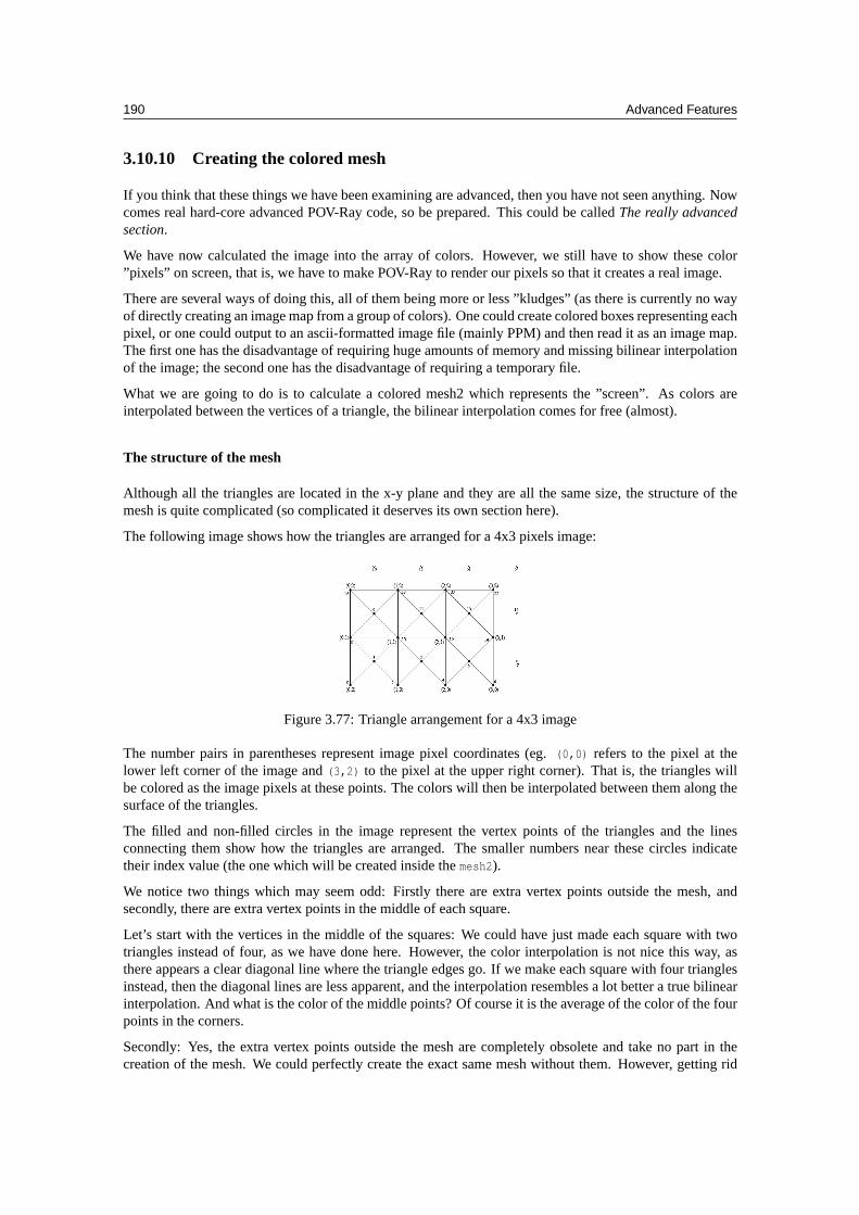
190 Advanced Features
3.10.10 Creating the colored mesh
If you think that these things we have been examining are advanced, then you have not seen anything. Nowcomes real hard-core advanced POV-Ray code, so be prepared. This could be calledThe really advancedsection.
We have now calculated the image into the array of colors. However, we still have to show these color”pixels” on screen, that is, we have to make POV-Ray to render our pixels so that it creates a real image.
There are several ways of doing this, all of them being more or less ”kludges” (as there is currently no wayof directly creating an image map from a group of colors). One could create colored boxes representing eachpixel, or one could output to an ascii-formatted image file (mainly PPM) and then read it as an image map.The first one has the disadvantage of requiring huge amounts of memory and missing bilinear interpolationof the image; the second one has the disadvantage of requiring a temporary file.
What we are going to do is to calculate a colored mesh2 which represents the ”screen”. As colors areinterpolated between the vertices of a triangle, the bilinear interpolation comes for free (almost).
The structure of the mesh
Although all the triangles are located in the x-y plane and they are all the same size, the structure of themesh is quite complicated (so complicated it deserves its own section here).
The following image shows how the triangles are arranged for a 4x3 pixels image:
Figure 3.77: Triangle arrangement for a 4x3 image
The number pairs in parentheses represent image pixel coordinates (eg.(0,0) refers to the pixel at thelower left corner of the image and(3,2) to the pixel at the upper right corner). That is, the triangles willbe colored as the image pixels at these points. The colors will then be interpolated between them along thesurface of the triangles.
The filled and non-filled circles in the image represent the vertex points of the triangles and the linesconnecting them show how the triangles are arranged. The smaller numbers near these circles indicatetheir index value (the one which will be created inside themesh2).
We notice two things which may seem odd: Firstly there are extra vertex points outside the mesh, andsecondly, there are extra vertex points in the middle of each square.
Let’s start with the vertices in the middle of the squares: We could have just made each square with twotriangles instead of four, as we have done here. However, the color interpolation is not nice this way, asthere appears a clear diagonal line where the triangle edges go. If we make each square with four trianglesinstead, then the diagonal lines are less apparent, and the interpolation resembles a lot better a true bilinearinterpolation. And what is the color of the middle points? Of course it is the average of the color of the fourpoints in the corners.
Secondly: Yes, the extra vertex points outside the mesh are completely obsolete and take no part in thecreation of the mesh. We could perfectly create the exact same mesh without them. However, getting rid
3.10 SDL tutorial: A raytracer 191
of these extra vertex points makes our lives more difficult when creating the triangles, as it would make theindexing of the points more difficult. It may not be too much work to get rid of them, but they do not takeany considerable amount of resources and they make our lives easier, so let’s just let them be (if you wantto remove them, go ahead).
Creating the mesh
What this means is that for each pixel we create two vertex points, one at the pixel location and one shiftedby ”0.5” in the x and y directions. Then we specify the color for each vertex points: For the even vertexpoints it is directly the color of the correspondent pixel; for the odd vertex points it is the average of thefour surrounding pixels.
Let’s examine the creation of the mesh step by step:
Creating the vertex points
#default { finish { ambient 1 } }
#debug "Creating colored mesh to show image...\n"mesh2{ vertex_vectors
{ ImageWidth*ImageHeight*2,#declare IndY = 0;#while(IndY < ImageHeight)
#declare IndX = 0;#while(IndX < ImageWidth)
<(IndX/(ImageWidth-1)-.5)*ImageWidth/ImageHeight*2,IndY/(ImageHeight-1)*2-1, 0>,
<((IndX+.5)/(ImageWidth-1)-.5)*ImageWidth/ImageHeight*2,(IndY+.5)/(ImageHeight-1)*2-1, 0>
#declare IndX = IndX+1;#end#declare IndY = IndY+1;
#end}
First of all we use a nice trick in POV-Ray: Since we are not using light sources and there is nothingilluminating our mesh, what we do is to set the ambient value of the mesh to 1. We do this by just makingit the default with the#default command, so we do not have to bother later.
As we saw above, what we are going to do is to create two vertex points for each pixel. Thus we knowwithout further thinking how many vertex vectors there will be:ImageWidth*ImageHeight*2
That was the easy part; now we have to figure out how to create the vertex points themselves. Each vertexlocation should correspond to the pixel location it is representing, thus we go through each pixel index(practically the number pairs in parentheses in the image above) and create vertex points using these indexvalues. The location of these pixels and vertices are the same as we assumed when we calculated the imageitself (in the previous part). Thus the y coordinate of each vertex point should go from -1 to 1 and similarlythe x coordinate, but scaled with the aspect ratio.
If you look at the creation of the first vector in the code above, you will see that it is almost identical to thedirection vector we calculated when creating the image.
The second vector should be shifted by 0.5 in both directions, and that is exactly what is done there. Thesecond vector definition is identical to the first one except that the index values are shifted by 0.5. Thiscreates the points in the middle of the squares.
192 Advanced Features
The index values of these points will be arranged as shown in the image above.
Creating the textures
texture_list{ ImageWidth*ImageHeight*2,
#declare IndY = 0;#while(IndY < ImageHeight)
#declare IndX = 0;#while(IndX < ImageWidth)
texture { pigment { rgb Image[IndX][IndY] } }#if(IndX < ImageWidth-1 \& IndY < ImageHeight-1)
texture { pigment { rgb(Image[IndX][IndY]+Image[IndX+1][IndY]+Image[IndX][IndY+1]+Image[IndX+1][IndY+1])/4 } }
#elsetexture { pigment { rgb 0 } }
#end#declare IndX = IndX+1;
#end#declare IndY = IndY+1;
#end}
Creating the textures is very similar to creating the vertex points (we could have done both inside the sameloop, but due to the syntax of themesh2 we have to do it separately).
So what we do is to go through all the pixels in the image and create textures for each one. The first textureis just the pixel color itself. The second texture is the average of the four surrounding pixels.
Note: we can calculate it only for the vertex points in the middle of the squares; for the extra vertex pointsoutside the image we just define a dummy black texture.
The textures have the same index values as the vertex points.
Creating the triangles
This one is a bit trickier. Basically we have to create four triangles for each ”square” between pixels. Howmany triangles will there be?
Let’s examine the creation loop first:
face_indices{ (ImageWidth-1)*(ImageHeight-1)*4,
#declare IndY = 0;#while(IndY < ImageHeight-1)
#declare IndX = 0;#while(IndX < ImageWidth-1)
...
#declare IndX = IndX+1;#end#declare IndY = IndY+1;
#end}
3.10 SDL tutorial: A raytracer 193
The number of ”squares” is one less than the number of pixels in each direction. That is, the numberof squares in the x direction will be one less than the number of pixels in the x direction. The same forthe y direction. As we want four triangles for each square, the total number of triangles will then be(ImageWidth-1)*(ImageHeight-1)*4.
Then to create each square we loop the amount of pixels minus one for each direction.
Now in the inside of the loop we have to create the four triangles. Let’s examine the first one:
<IndX*2+ IndY *(ImageWidth*2),IndX*2+2+IndY *(ImageWidth*2),IndX*2+1+IndY *(ImageWidth*2)>,IndX*2+ IndY *(ImageWidth*2),IndX*2+2+IndY *(ImageWidth*2),IndX*2+1+IndY *(ImageWidth*2),
This creates a triangle with a texture in each vertex. The first three values (the indices to vertex points) areidentical to the next three values (the indices to the textures) because the index values were exactly the samefor both.
TheIndX is always multiplied by 2 because we had two vertex points for each pixel andIndX is basicallygoing through the pixels. LikewiseIndY is always multiplied byImageWidth*2 because that is how long arow of index points is (ie. to get from one row to the next at the same x coordinate we have to advanceImageWidth*2 in the index values).
These two things are identical in all the triangles. What decides which vertex point is chosen is the ”+1”or ”+2” (or ”+0” when there is nothing). ForIndX ”+0” is the current pixel, ”+1” chooses the point in themiddle of the square and ”+2” chooses the next pixel. ForIndY ”+1” chooses the next row of pixels.
Thus this triangle definition creates a triangle using the vertex point for the current pixel, the one for thenext pixel and the vertex point in the middle of the square.
The next triangle definition is likewise:
<IndX*2+ IndY *(ImageWidth*2),IndX*2+ (IndY+1)*(ImageWidth*2),IndX*2+1+IndY *(ImageWidth*2)>,IndX*2+ IndY *(ImageWidth*2),IndX*2+ (IndY+1)*(ImageWidth*2),IndX*2+1+IndY *(ImageWidth*2),
This one defines the triangle using the current point, the point in the next row and the point in the middle ofthe square.
The next two definitions define the other two triangles:
<IndX*2+ (IndY+1)*(ImageWidth*2),IndX*2+2+(IndY+1)*(ImageWidth*2),IndX*2+1+IndY *(ImageWidth*2)>,IndX*2+ (IndY+1)*(ImageWidth*2),IndX*2+2+(IndY+1)*(ImageWidth*2),IndX*2+1+IndY *(ImageWidth*2),
<IndX*2+2+IndY *(ImageWidth*2),IndX*2+2+(IndY+1)*(ImageWidth*2),IndX*2+1+IndY *(ImageWidth*2)>,IndX*2+2+IndY *(ImageWidth*2),IndX*2+2+(IndY+1)*(ImageWidth*2),IndX*2+1+IndY *(ImageWidth*2)

194 Advanced Features
3.10.11 The Camera-setup
The only thing left is the camera definition, so that POV-Ray can calculate the image correctly:
camera { orthographic location -z*2 look_at 0 }
Why ”2”? As the defaultdirection vector is<0,0,1> and the defaultup vector is<0,1,0> and we wantthe up direction to cover 2 units, we have to move the camera two units away.
Chapter 4
Questions and Tips
This section contains answers to frequently asked questions about POV-Ray as well as many useful tips notcovered in other parts of this documentation.
While it was current at the time that this POV-Ray documentation help file was created, it will almostcertainly be out of date by the time you are reading this. So, if you do not find an answer to your questionhere, please check out the current version1 on the internet.
If you have some question not answered in this FAQ, do not be afraid to contact the TAG2 or ask in theproper group of the POV-Ray news-server3.
4.1 Language Tips and tricks to achieve useful things
4.1.1 How do I make a visible light source?
”How do I make a visible light source?”or: ”Although I put the camera just in front of my light source, Icannot see anything. What am I doing wrong?”
A light source in POV-Ray is only a concept. When you add a light source to the scene, you are actuallysaying to POV-Ray ”hey, there is light coming from this point”. As the name says, it is a lightsource, nota physical light (like a light bulb or a bright spot like a star). POV-Ray does not add anything to that placewhere the light is coming, ie. there is nothing there, only empty space. It is just a kind of mathematicalpoint POV-Ray uses to make shading calculations.
To make the light source visible, you have to put something there. There is alooks like keyword in thelight source block which allows to easily attach an object to the light source. This object implicitly doesnot cast any shadows. You can make something like this:
light_source{ <0,0,0> color 1
looks_like{ sphere
{ <0,0,0>,0.1color { rgb 1 }finish { ambient 1 }
}
1http://www.povray.org/search/redirect?VFAQ2http://tag.povray.org/3news://news.povray.org
196 Questions and Tips
}translate <10,20,30>
}
It is a good idea to define both things, the light source and the lookslike object, at the origin, and thentranslate them to their right place.
Note also the ’finish { ambient 1 }’ which makes the sphere to apparently glow (see also the next ques-tion).
You can also get visible light sources using other techniques: Media, lens flare (available as 3rd partyinclude file), glow patch, etc.
4.1.2 How do I make bright objects?
”How do I make bright objects, which look like they are emitting light?”
There is a simple trick to achieve this: Set the ambient value of the object to 1 or higher. This makesPOV-Ray to add a very bright illumination value to the object so the color of the object is in practice takenas is, without darkening it due to shadows and shading. This results in an object which seems to glow lightby itself even if it is in full darkness (useful to make visible light sources, or small lights like leds which donot cast any considerable light to their surroundings but can be easily seen even in the darkness).
A more sophisticated method would be using an emitting media inside the object (and making the objectitself transparent or semi-transparent).
4.1.3 How do I move the camera in a circular path?
”How do I move the camera in a circular path while looking at the origin?”
There are two ways to make this: The easy (and limited) way, and the more mathematical way.
The easy way:
camera{ location <0,0,-10>
look_at 0rotate <0,clock*360,0>
}
This puts the camera at 10 units in the negative Z-axis and then rotates it around the Y-axis while lookingat the origin (it makes a circle of radius 10).
The mathematical way:
camera{ location <10*sin(2*pi*clock),0,-10*cos(2*pi*clock)>
look_at 0}
This makes exactly the same thing as the first code, but this way you can control more precisely the path ofthe camera. For example you can make the path elliptical instead of circular by changing the factors of thesine and the cosine (for example instead of 10 and 10 you can use 10 and 5 which makes an ellipse with themajor radius 10 and minor radius 5).
An easier way to do the above is to use the vrotate() function, which handles the sin() and cos() stuff foryou, as well as allowing you to use more complex rotations.
4.1 Language Tips and tricks to achieve useful things 197
camera{ location vrotate(x*10, y*360*clock)
look_at 0}
To get an ellipse with this method, you can just multiply the result from vrotate by a vector, scaling theresulting circle. With the last two methods you can also control the lookat vector (if you do not want itlooking just at the origin).
You could also do more complex transformations combining translate, scale, rotate, and matrix transformsby replacing the vrotate() call with a call of the vtransform() function found infunctions.inc (new inPOV-Ray 3.5).
4.1.4 How do I use an image to texture my object?
The answer to this question can be easily found in the POV-Ray documentation, so I will just quote thesyntax:
pigment{ image_map
{ gif "image.gif"map_type 1
}}
(Note that in order for the image to be aligned properly, either the object has to be located at the origin whenapplying the pigment or the pigment has to be transformed to align with the object. It is generally easiest tocreate the object at the origin, apply the texture, then move it to wherever you want it.)
Substitute the keywordgif with the type of image you are using (if it is not a GIF):tga, iff, ppm, pgm,
png or sys.
A map type 0 gives the default planar mapping.A map type 1 gives a spherical mapping (maps the image onto a sphere).With map type 2 you get a cylindrical mapping (maps the image onto a cylinder).Finally map type 5 is a torus or donut shaped mapping (maps the image onto a torus).
See the documentation for more details.
4.1.5 How can I generate a spline?
”How can I generate a spline, for example for a camera path for an animation?”
POV-Ray 3.6 has a splines feature that allows you to create splines. This is covered in the documentationand there are demo files showing examples of use. There exist also third party include files for splinegeneration that have greater flexibility than the internal splines, for example the spline macros by ChrisColefax4.
4.1.6 How can I simulate motion blur?
The official POV-Ray 3.6 does not support motion blur calculations, but there are some patched versionswhich do.
4http://www.geocities.com/ccolefax/spline/index.html
198 Questions and Tips
You can also use other tools to make this. One way to simulate motion blur is calculating a small animationand then averaging the images together. This averaging of several images can be made with third partyprograms, such as the Targa Averager program5.
4.1.7 How can I find the size of a text object?
”How can I find the size of a text object / center text / justify text?”
You can use themin extent() andmax extent() functions to get the corners of the bounding box of anyobject. While this is sometimes not the actual size of the object, for text objects this should be fairlyaccurate, enough to do alignment of the text object.
4.1.8 How do I make extruded text?
POV-Ray has true type font support built in that allows you to have 3D text in your scenes (see the docu-mentation about the ’text’ object for more details).
There are also some outside utilities that will import true type fonts and allow user manipulation on the text.One of these programs is called Elefont.
4.1.9 How do I make an object hollow?
This question usually means ”how do I make a hollow object, like a waterglass, a jug, etc”.
Before answering that question, let me explain some things about how POV-Ray handles objects:
Although the POV-Ray documentation talks about ”solid” and ”hollow” objects, that is not how it actuallyworks. ”Solid” and ”hollow” are a bit misleading terms to describe the objects. You can also make an object”hollow” with that same keyword, but it is not that simple.
Firstly: POV-Ray only handles surfaces, not solid 3D-objects. When you specify a sphere, it is actually justa spherical surface. It is only a surface and it is not filled by anything. This can easily be seen by puttingthe camera inside the sphere or by clipping a hole to one side of the sphere with the clippedby keyword (soyou can look inside).
People often think that POV-Ray objects are solid, really 3D, with solid material filling the entire objectbecause they make a ’difference’ CSG object and it seems like the object is actually solid. What the’difference’ CSG actually does is to cut away a part of the object andadd a new surfacein the place ofthe hole, which completely covers the hole, so you cannot see inside the object (this new surface is actuallythe part of the second object which is ”inside” the first object). Again, if you move the camera inside theobject, you will see that actually it is hollow and the object is just a surface.
So what is all this ”solid” and ”hollow” stuff the documentation talks of, and what is the ”hollow” keywordused for?
Although objects are actually surfaces, POV-Ray handles them as if they were solid. For example, fog andmedia do not go inside solid objects. If you put a glass sphere into the fog, you will see that there is no foginside the sphere.
If you add the ”hollow” keyword to the object, POV-Ray will no longer handle it as solid, so fog andatmosphere will invade the inside of the object. This is the reason why POV-Ray issues a warning whenyou put the camera inside a non-hollow object (because, as it says, fog and other atmospheric effects maynot work as you expected).
5http://iki.fi/warp/PovUtils/average/
4.1 Language Tips and tricks to achieve useful things 199
If your scene does not use any atmospheric effect (fog or media) there is not any difference between a”solid” or ”hollow” object.
So all the objects in POV-Ray are hollow. But the surface of the objects is always infinitely thin, and thereis only one surface. With real world hollow objects you have always two surfaces: an outer surface and aninner surface.
Usually people refer to these kind of objects when they ask for hollow objects. This kind of objects areeasily achieved with a ’difference’ CSG operation, like this:
// A simple water glass made with a difference:difference{ cone { <0,0,0>,1,<0,5,0>,1.2 }
cone { <0,.1,0>,.9,<0,5.1,0>,1.1 }texture { Glass }
}
The first cone limits the outer surface of the glass and the second cone limits the inner surface.
4.1.10 How can I fill a glass with water or other objects?
As described in the ”hollow objects” question above, hollow objects have always two surfaces: an outersurface and an inner surface. If we take the same example, a simple glass would be like:
// A simple water glass made with a difference:#declare MyGlass=difference{ cone { <0,0,0>,1,<0,5,0>,1.2 }
cone { <0,.1,0>,.9,<0,5.1,0>,1.1 }texture { Glass }
}
The first cone limits the outer surface of the glass and the second cone limits the inner surface.
If we want to fill the glass with water, we have to make an object which coincides with the inner surfaceof the glass. Note that you have to avoid the coincident surfaces problem so you should scale the ”water”object just a little bit smaller than the inner surface of the glass. So we make something like this:
#declare MyGlassWithWater=union{ object { MyGlass }
cone{ <0,.1,0>,.9,<0,5.1,0>,1.1
scale .999texture { Water }
}}
Now the glass is filled with water. But there is one problem: There is too much water. The glass shouldbe filled only up to certain level, which should be definable. Well, this can be easily made with a CSGoperation:
#declare MyGlassWithWater=union{ object { MyGlass }
intersection{ cone { <0,.1,0>,.9,<0,5.1,0>,1.1 }
plane { y,4 }scale .999
200 Questions and Tips
texture { Water }}
}
Now the water level is at a height of 4 units.
4.1.11 How can I bend a object?
There is no direct support for bending in POV-Ray, but you can achieve acceptable bending with the ObjectBender by Chris Colefax6.
Some objects can be ”bent” by just modelling it with other objects. For example a bent cylinder can bemore easily (and accurately) achieved using the intersection of a torus and some limiting objects.
It might be a bit strange why most renderers support bending but POV-Ray does not. To understand thisone has to know how other renderers (the so-called ”scanline-renderers” work):
In the so-called ”scanline renders” all objects are modelled with triangle meshes (or by primitives suchas NURBS or bezier patches which can be very easily converted to triangles). The ”bending” is, in fact,achieved by moving the vertices of the triangles.
In this context the term ”bending” is a bit misleading. Strictly speaking, bending a triangle mesh would alsobend the triangles themselves, not only move their vertices. No renderer can do this. (It can be, however,simulated by splitting the triangles into smaller triangles, and so the ”bending” effect is more accurate,although not yet perfect.) What these renderers do is not a true bending in the strict mathematical sense, butonly an approximation achieved by moving the vertices of the triangles.
This difference might sound irrelevant, as the result of this kind of ”fake” bending usually looks as good asa true bending. However, it is not irrelevant from the point of view of POV-Ray. This is because POV-Raydoes not represent the objects with triangles, but they are true mathematical surfaces. POV-Ray cannot”fake” a bending by moving vertices because there are no vertices to move. In practice bending (and othernon-linear transformations) would require the calculation of the intersection of the object surface and acurve (instead of a straight line), which is pretty hard and many times analytically not possible.
Note that isosurface objects can be modified with proper functions in order to achieve all kinds of transfor-mations (linear and non-linear) and thus they are not really bound to this limitation. However, achievingthe desired transformation needs some knowledge of mathematics.
See also the variable ior question.
4.1.12 Can I get non-grainy focal blur?
”The focal blur is very grainy. Can I get rid of the graininess?”
Yes. Setvariance to 0 (or to a very small value, like for example 1/100000) and choose a high enoughblur samples. The rendering will probably slow down quite a lot, but the result should be very good.
4.2 Language Things that don’t work as one expects
4.2.1 Using several transparent objects makes them black?
”When I put several transparent objects one in front of another or inside another, POV-Ray calculates afew of them, but the rest are completely black, no matter what transparency values I give.”
6http://www.geocities.com/SiliconValley/Lakes/1434/bend.html
4.2 Language Things that don’t work as one expects 201
Short answer: Try increasing themax trace level value in theglobal settings block (the default is 5).
Long answer:
Raytracing has a peculiar feature: It can calculate reflection and refraction. Each time a ray hits the surfaceof an object, the program looks if this surface is reflective and/or refractive. If so, it shoots another ray fromthis point to the appropriate direction.
Now, imagine we have a glass sphere. Glass reflects and refracts, so when the ray hits the sphere, twoadditional rays are calculated, one outside the sphere (for the reflection) and one inside (for the refraction).Now the inside ray will hit the sphere again, so two new rays are calculated, and so on and so on...
You can easily see that there must be a maximum number of reflections/refractions calculated, becauseotherwise POV-Ray would calculate that one pixel forever.
This number can be set with themax trace level option in theglobal settings block. The default valueis 5, which is enough for most scenes. Sometimes it is not enough (specially when there are lots ofsemitransparent objects one over another) so you have to increase it.
So try something like:
global_settings{
max_trace_level 10}
4.2.2 I’m getting color banding in the image
”When I make an image with POV-Ray, it seems to use just a few colors since I get color banding orconcentric circles of colors or whatever where it should not. How can I make POV-Ray to use more colors?”
POV-Ray always writes true color images (ie. with 16777216 colors, ie. 256 shades of red, 256 shades ofgreen and 256 shades of blue) (this can be changed when outputting to PNG or to B/W TGA but this isirrelevant when answering to this question).
So POV-Ray is not guilty. It always uses the maximum color resolution available in the target image fileformat.
This problem usually happens when you are using windows with 16-bit colors (ie. only 65536 colors, theso-called hicolor mode) and open the image created by POV-Ray with a program which does not dither theimage. The image is still true color, but the program is unable to show all the colors, but shows only 65536of them (dithering is a method that ”fakes” more colors by mixing pixels of two adjacent colors to simulatethe in-between colors).
So the problem is not in POV-Ray, but in your image viewer program. Even if POV-Ray shows a poorimage while rendering because you have a resolution with too few colors, the image file created will havefull color range.
4.2.3 Rotation behaves very strangely
”When I rotate an object, it dissapears from the image or moves very strangely. Why?”
You need to understand how rotation works in POV-Ray.
Objects arealwaysrotated around the axes. When you rotate, for example,<20,0,0>, that means that youare rotating around the X-axis 20 degrees (counter-clockwise). This is independent of the location of theobject: It always rotates around the axis (what is the center of the object anyways? how do you locate it?).
202 Questions and Tips
This means that if the object is not centered in the axis, it will orbit this axis like the Moon orbits the Earth(showing always the same side to the Earth).
It is a very good practice to define all objects centered at the origin (ie. its ’center’ is located at<0,0,0>).Then you can rotate it arbitrarily. After this you can translate it to its proper location in the scene. It is agood idea to do this to every object even if you do not rotate it (because you cannot never say if you willrotate it some day nevertheless).
What if, after all, you have a very complex object defined, but its center is not at the origin, and you wantto rotate it around its center? Then you can just translate it to the origin, rotate it and then translate it backto its place. Suppose that the center of the object is located at<10,20,-30>; you can rotate it this way:
translate -<10,20,-30>rotate <whatever>translate <10,20,-30>
4.2.4 The image gets distorted when rendering a square image
”If I tell POV-Ray to render a square image or otherwise change the aspect ratio, the output image isdistorted. What am I doing wrong?”
The problem is that the camera is set to an aspect ratio of 4/3, while the picture you are trying to render hasan aspect ratio of 1/1 (or whatever).
You can set the aspect ratio with the ’right’ keyword in the camera block. The general way to set the correctaspect ratio for your image dimensions is:
camera{ right x*ImageWidth/ImageHeight
(other camera settings...)}
This keyword can also be used to change the handedness of POV-Ray (see the question about Moray andPOV-Ray handedness for more details).
Note: One could think ”why does not POV-Ray always set automatically the aspect ratio of the cameraaccording to the resolution of the image?”.
There is one thing wrong in this thought: It assumes that pixels are always square (ie. the aspect ratio of thepixels is 1/1). The logic of this behaviour comes clear with an example:
Suppose that you design a scene using a regular 4/3 aspect ratio, as usual (like 320x240, 640x480 and soon). This image is designed to look good when viewing in a 4/3 monitor (as they all are in home computers).
Now you want to render this image for the Windows startup image. The resolution of the Windows startupimage is 320x400. This resolution has not an aspect ratio of 4/3 and the pixels are not square (the pixels havean aspect ratio of 1/0.6 instead of 1/1). Now, when you render your image at a resolution of 320x400 withPOV-Ray and show it with the monitor set to that resolution (as it is set at windows startup when the startupimage is shown), the aspect ratio will be the correct one so the image will have the correct proportions (andit will not be squeezed in any direction).
If you had changed the aspect ratio of the camera to 320/400 (instead of using the default 4/3) you wouldnot only have got a different image (showing parts of the scene not shown in the original or hiding partsvisible in the original), but it would have looked sqeezed when shown in the 320x400 screen resolution.
Thus, the camera aspect ratio is the aspect ratio of the final image on screen, when viewed in the finalresolution (which might not be a 4/3-resolution). Since the monitor screen has an aspect ratio of 4/3, this isthe default for the camera as well.
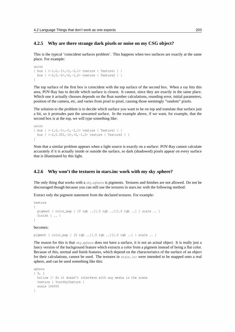
4.2 Language Things that don’t work as one expects 203
4.2.5 Why are there strange dark pixels or noise on my CSG object?
This is the typical ’coincident surfaces problem’. This happens when two surfaces are exactly at the sameplace. For example:
union{ box { <-1,0,-1>,<1,-2,1> texture { Texture1 } }
box { <-2,0,-2>,<2,-1,2> texture { Texture2 } }}
The top surface of the first box is coincident with the top surface of the second box. When a ray hits thisarea, POV-Ray has to decide which surface is closest. It cannot, since they are exactly in the same place.Which one it actually chooses depends on the float number calculations, rounding error, initial parameters,position of the camera, etc, and varies from pixel to pixel, causing those seemingly ”random” pixels.
The solution to the problem is to decide which surface you want to be on top and translate that surface justa bit, so it protrudes past the unwanted surface. In the example above, if we want, for example, that thesecond box is at the top, we will type something like:
union{ box { <-1,0,-1>,<1,-2,1> texture { Texture1 } }
box { <-2,0.001,-2>,<2,-1,2> texture { Texture2 } }}
Note that a similar problem appears when a light source is exactly on a surface: POV-Ray cannot calculateaccurately if it is actually inside or outside the surface, so dark (shadowed) pixels appear on every surfacethat is illuminated by this light.
4.2.6 Why won’t the textures in stars.inc work with my sky sphere?
The only thing that works with asky sphere is pigments. Textures and finishes are not allowed. Do not bediscouraged though because you can still use the textures in stars.inc with the following method:
Extract only the pigment statement from the declared textures. For example:
texture{
pigment { color_map { [0 rgb ..][.5 rgb ..][1.0 rgb ..] } scale .. }finish { .. }
}
becomes:
pigment { color_map { [0 rgb ..][.5 rgb ..][1.0 rgb ..] } scale .. }
The reason for this is thatsky sphere does not have a surface, it is not an actual object. It is really just afancy version of the background feature which extracts a color from a pigment instead of being a flat color.Because of this, normal and finish features, which depend on the characteristics of the surface of an objectfor their calculations, cannot be used. The textures instars.inc were intended to be mapped onto a realsphere, and can be used something like this:
sphere{ 0, 1
hollow // So it doesn’t interfere with any media in the scenetexture { YourSkyTexture }scale 100000
}
204 Questions and Tips
4.2.7 When I use filter or transmit with my .tga image map nothing happens.
POV-Ray can only apply filter or transmit to 8 bit 256 color palleted images. Since most.tga, .png, and.bmp images are 24bit and 16 million colors they do not work with filter or transmit. If you must use filteror transmit with your image maps you must reduce the color depth to a format the supports 256 colors suchas the.gif image format.
You might also check the POV-Ray docs on using the alpha channel of.png files if you need specific areasthat are transparent.
4.2.8 Isosurface not rendering properly?
”My isosurface is not rendering properly: there are holes or random noise or big parts or even the wholeisosurface just disappears.”
The most common reason for these type of phenomena with isosurfaces is a too lowmax gradient value.Useevaluate to make POV-Ray calculate a propermax gradient for the isosurface (remember to specify asensiblemax gradient even when you useevaluate or else the result may not be correct).
Sometimes a too highaccuracy value can also cause problems even when themax gradient is ok. If playingwith the latter does not seem to help, try also lowering theaccuracy.
Remember that specifying amax gradient which is too high for an isosurface, although it gives the correctresult, is needlessly slow, so you should always calculate the propermax gradient for each isosurface youmake.
Note that there are certain pathological functions where nomax gradient or accuracy will help. Thesefunctions usually have discontinuities or similar ”ill-behaving” properties. With those you just have to finda solution which gives the best quality/speed tradeoff. Isosurfaces work best with functions which givesmooth surfaces.
4.3 Language related things
4.3.1 How do I turn animation on?
”How do I turn animation on? I have used theclock -variable in my scene, but POV-Ray still onlycalculates one frame.”
The easiest way is to just specify the appropriate command line parameter on the command line or in thecommand line field in the rendering settings menu (in the Windows version). For example, if you want tocreate 20 frames, type this:+kff20
This will create 20 frames with theclock variable going from 0 to 1. The other command line parametersare found in the POV-Ray documentation.
Ken Tyler has also another good solution for this:
In the directory that you installed POV-Ray into you will find a subdirectory called scenes and anotherinside that called animate. You will find several example files showing you how to write your scene to usethe clock variable. You will still need to activate POV-Ray’s animation feature by using an.ini file withthe correct info or with command line switches. I personaly like to use the ini file method. If you try thisopen the masterpovray.ini file from the tools menu and add the following lines:
;clock=1;Initial_Frame=1
4.3 Language related things 205
;Final_Frame=20;Cyclic_Animation = on;Subset_Start_Frame=6;Subset_End_Frame=9
Save the file and close it. When you need to use the animation feature simply go in and edit thepovray.ini
file and uncomment out the functions you want to use. At a minimum you will need to use theinitial -
frame andfinal frame option to make it work. Once you have stopped rendering your series of frames besure to comment out the clock variables in the ini file. After you have rendered a series of individual framesyou will still need to compile them into the animation format that you wish to use such as AVI or MPEG.See our links collection on our website7 for programs that can help you do this. POV-Ray has no internalability to do this for you except on the Macintosh platform of the program.
The Mac version normally does not use.ini files and lacks any command line, but uses a completelygraphical interface instead. To activate animation, choose the render settings item from the Edit menu(right under ”Preferences”, it will be titled ”FILENAME Settings”, where FILENAME is the name of yourfile), click on the Animation tab, and enter the needed information in the text boxes.
4.3.2 Can POV-Ray use multiple processors?
Short answer: The only way to run POV-Ray on multiple processors is to run several copies of POV-Ray.
Long answer:
Making a program use multiple threads is not as trivial as it may sound. Here are some reasons why it isquite difficult to make with POV-Ray:
• You cannot do it with standard C (nor C++), and POV-Ray is intended to be very portable. This is notjust an issue of philosophy or purism, POV-Ray is really used on a large variety of different platforms.
• Multithreading is a very complex issue and it is much more difficult to make a bugless multithreadedprogram than a single-threaded (there are several things in multithreading, like mutual exclusionproblems, which make the multithreaded program very non-deterministic). It is not impossible,though, since it has been done (there are patched versions of POV-Ray with multithreading support).However, it is far from trivial.
• Raytracing is usually thought as an easily threaded problem. You just calculate one pixel and draw iton screen, independent of the other pixels. However, with advanced techniques, like antialiasing andspecially stochastic global illumination calculation (referred as ”radiosity” in POV-Ray’s documen-tation and syntax) this is not true anymore.
– To speed up antialiasing, a threshold value is used between pixels. If the difference in colorbetween two pixels is higher than the threshold, then antialiasing is calculated. Of course weneed info from the nearby pixels for this.
– In global illumination calculations lighting values are stored in a spatial tree structure. Thefollowing pixels may use the information stored in this tree for their illumination. This meansthat the pixel calculation at the upper left corner may affect on the color of the pixel in the lowerright corner. This is the reason why calculating a radiosity image in parts does not work verywell.
Both problems can probably be solved in some way, but as said, it is far from trivial.
An excellent article about the issue can be found on the Ray Tracing News web page8.
Here is an answer from John M. Dlugosz with useful tips:
7http://povray.org/links/3DAnimation Utilities/8http://www.acm.org/tog/resources/RTNews/html/rtnv12n2.html#art3
206 Questions and Tips
The POV-Ray rendering engine is a single thread of execution, so when run on a dual Pentium Pro (runningNT4) the CPU indicator only goes up to about 50%. POV does not use more than half the available poweron the machine.
That is the basic issue, though to quibble a bit it is not exactly true: the rendering engine soaks up one wholeCPU, but the editor runs on its own thread, and operating system functions (writing to the file, updating thedisplay, network activity, system background tasks) run on different threads. This gives a little bit of abonus, and the system uses as much as 54% of available MIPS when watching it. More importantly, themachine is still highly responsive, and editing or other applications continue on without being sluggish.
But for a long render, it is annoying to have one CPU be mostly idle. What can be done to cut renderingtime in half (from 20 hours down to 10, for example)?
The simplest thing is to run two copies of POV on the machine. Have one copy render the top half, and theother render the bottom half. Then paste the halves together in your picture editor.
One thing to watch out for: do not just fire up two copies and point them at the same INI file and image file.They will overwrite each other’s output and make a big mess. Instead, you must make sure each is writingto a different file.
For moderate renders, you might let one copy chug away on the long render, and use a second copyinteractivly to continue development in POV.
4.3.3 Can I get a wireframe render of my scene?
”Is there a way to generate a wireframe output image from a POV scene file?”
Short answer: No.
Long answer:
You have to understand the difference between a modeller like 3D-Studio and POV-Ray in the way they han-dle objects. Those modellers always use triangle meshes (and some modellers use also NURBS which canbe very easily converted into triangles). Triangle meshes are extremely simple to represent in a wireframeformat: Just draw a line for each triangle side.
However, POV-Ray handles most of the objects as mathematical entities, not triangle meshes. When youtell POV-Ray to create a sphere, POV-Ray only handles it as a point and a radius, nothing else (besidesthe possible matrix transform applied to it). POV-Ray only has a notion of the shape of the object as amathematical formula (it can calculate the intersection of a line and the sphere).
For wireframe output there should be a way to convert that mathematical representation of the object intoactual triangles. This is called tesselation.
For some mathematical objects, like the sphere, the box, etc, tesselation is quite trivial. For other entities,like CSG difference, intersection, etc, it is more difficult (although not impossible). For other entities itis completely impossible: infinite non-flat surfaces like paraboloids and hyperboloids (well, actually it ispossible if you limit the size of the surface to a finite shape; still the amount of triangles that needs to becreated would be extremely high).
There have been lots of discussions about incorporating tesselation into POV-Ray. But since POV-Rayis just a renderer, not a modeller, it does not seem to be worth the efforts (adding tesselation to all theprimitives and CSG would be ahuge job).
(Of course tesselation could give some other advantages, like the ability to fake non-uniform transforma-tions to objects like most triangle mesh modellers do...)
If you just want fast previews of the image, you can try to use the quality parameter of POV-Ray. Forexample setting quality to 0 (+q0) can give a very fast render. See also the rendering speed question.
4.3 Language related things 207
4.3.4 Can I specify variable IOR for an object?
”Can I specify variable IOR for an object? Is there any patch that can do this? Is it possible?”
Short answer: No.
Long answer:
There are basically two ways of defining variable IOR for an object: IOR changing on the surface of theobject and IOR changing throughout inside the object.
The first one is physically incorrect. For uniform IOR it simulates physical IOR quite correctly since forobjects with uniform density the light bends at the surface of the object and nowhere else. However if thedensity of the object is not uniform but changes throughout its volume, the light will bend inside the object,while travelling through it, not only on the surface of the object.
This is why variable IOR on the surface of the object is incorrect and the possibility of making this wasremoved in POV-Ray 3.1.
From this we can deduce that a constant IOR is kind of property of the surface of the object while variableIOR is a property of the interior of the object (like media in POV-Ray). Of course the physically correctinterpretation of this phenomenon is that IOR is always a property of the whole object (ie. its interior), notonly its surface (and this is why IOR is now a property of the interior of the object in POV-Ray); however,the effect of a constant IOR has effect only at the surface of the object and this is what POV-Ray does whenbending the rays.
The correct simulation for variable IOR, thus, would be to bend the ray inside the object depending on thedensity of the interior of the object at each point.
This is much harder to do than one may think. The reasons are similar to why non-uniform transformationsare too difficult to calculate reasonably (as far as I know there exists no renderer that calculates true non-uniform transformations; mesh modellers just move the vertices, they do not actually transform the object;a true non-uniform transformation would bend the triangles). Moreover: Non-uniform transformations canbe faked if the object is made of many polygons (you can move the vertices as most mesh modellers do),but you cannot fake a variable IOR in this way.
Variable IOR is (mostly) impossible to calculate analytically (ie. in a mathematically exact way) at least ina reasonable time. The only way would be to calculate it numerically (usually by super-sampling).
Media in POV-Ray works in this way. It does not even try to analytically solve the color of the media, butsupersamples the media along the ray and averages the result. This can be pretty inaccurate as we can seewith the media method 1 (the only one which was supported in POV-Ray 3.1). However some tricks canbe used to make the result more accurate without having to spend too much time, for example antialiasing(which is used by the media method 3). This is a quite easy calculation because the ray is straight, POV-Rayknows the start and end points of the ray and it knows that it does not intersect with anything along the ray(so it does not have to make ray-object intersection calculations while supersampling).
Variable IOR is, however, a completely different story. Here the program would have to shoot a LOT ofrays along the path of the bending light ray. For each ray it would have to make all the regular ray-objectintersection calculations. It is like having hundreds or thousands of transparent objects one inside another(with max tracelevel set so high that the ray will go through all of them). You can easily test how slow thisis. It is very slow.
One could think that ”hey, why not just shoot a few tens of rays and then use some kind of antialiasing toget the fine details, like in media method 3”.
Well, it might work (I have never seen it tested), but I do not think it will help much. The problem isthe inaccuracy of the supersampling (even when using antialiasing). In media it is not a big problem; ifa very small shadowed area in the media is not detected by the supersampling process, the result will not
208 Questions and Tips
differ very much from the correct one (since the shadowed area was so small it would have diminished thebrightness of that ray just a bit but no more) and it will probably still look good.
With IOR this is not anymore true. With IOR even very, very small areas may have very strong effect inthe end result, since IOR can drastically change the direction of the ray thus making the result completelydifferent (even very small changes can have great effect if the object behind the current refracting object isfar away).
This can have disastrous effects. The ior may change drastically from pixel to pixel almost at random, notto talk from frame to frame in an animation.To get a more or less accurate result lots of rays would be needed; just a few rays is not enough. Andshooting lots of rays is an extremely slow process.
4.3.5 What is Photon Mapping?
Photon mapping uses forward raytracing (ie. sending rays from light sources) calculate reflecting andrefracting light (aka. caustics).
The following is from the homepage of the developer (Nathan Kopp):
”My latest fun addition to POV is the photon map. The basic goal of this implementation of the photon mapis to render true reflective and refractive caustics. The photon map was first introduced by Henrik WannJensen. It is a way to store light information gathered from a backwards ray-tracing [sic] step in a datastructure independent from the geometry of a scene.”
It is surprisingly fast and efficient. How is this possible when forward raytracing is so inefficient? Forseveral reasons:
1. Photon mapping is only used to calculate illumination, ie. lighting values, not to render the actualscene. Lighting values do not have to be as accurate as the actual rendering (it does not matter if yourreflected light ”bleeds” a bit out of range; actually this kind of ”bleeding” happens in reality as well(due to light diffusing from air), so the result is not unrealistic at all).
2. Photon mapping is calculated only for those (user-specified) objects that need it (ie. objects that havereflection and/or refraction).
3. The rays are not shot to all directions, towards the entire scene, but only towards those specifiedobjects. Many rays are indeed shot in vain, without them affecting the final image in any way, butsince the total amountof rays shot is relatively small, the rendering time does not get inacceptablylonger.
4. The final image itself is rendered with regular backwards raytracing (the photon mapping is a precal-culation step done before the actual rendering). The raytracer does not need to use forward raytracingin this process (it just uses the precalculated lighting values which are stored in space).
As you have seen, for the photon mapping to work in an acceptable way, you have to tell the program whichobjects you want to reflect/refract light and which you do not. This way you can optimize a lot the photonmapping step.
4.4 File Formats
4.4.1 Saving the image to disk.
”I have rendered an image with POV-Ray, but how do I save it to JPG or GIF or any other image format?”
This is a typical problem of people using the Windows version of the program for first time.
4.4 File Formats 209
POV-Ray is a raytracer which has only one purpose: To read a source file describing the scene to raytraceand then calculate it and save it to disk in a supported image format, usually TGA (and optionally PNG,BMP, etc).
POV-Ray has always had this goal, and still has, and will (desirably) never change. It is mostly command-line oriented. It supports non-essential things, like showing the image while it is rendering.
A GUI does not change anything. POV-Ray is still POV-Ray, with or without GUI. It takes a source codeand calculates the image and saves it to disk. By default it shows the image while it is raytracing it, but thatis just a secondary feature, non-essential, irrelevant. It can be turned off and POV-Ray will still make itsjob.
So the answer to the question is: The imageis already savedon disk.
Usually it is saved in TGA or BMP format (it depends on the settings) with the same name as the sourcecode (so if the source is namedCHAIR.POV, the image will be namedCHAIR.TGA or CHAIR.BMP or whatever).The location is either the same directory where the.pov-file is or else a common directory for images(which you can set up in the main povray.ini file).
4.4.2 Can I convert my POV-Ray scenes to another format?
(Answer by Johannes Hubert)
For POV-Ray 2.2: Try Crossroads9 or if you want to convert to Moray MDL files, try POV2MDL10 fromThomas Baier.
For POV-Ray 3.1 and newer: There is unfortunately not much you can do. There is no real versatile programyet, that can read (and convert) POV-Ray 3.1 scripts (except for POV-Ray itself :-). Your best shots wouldbe: POV2RIB11 if you want to convert to the RIB format. If you know how to program C++, you can getthe ParPov C++ library from the same URL. It is a class-library for reading POV 3.1 scripts and convertingthem to C++ objects (it also has been used for POV2RIB).
3DWin from Thomas Baier (see the URL above) converts from the POB format to a lot of other formats.POB is a special binary POV-Ray format devised by Thomas and is written by a custom-compile version ofPOV-Ray 3.0 (get the POB-SDK at the same URL): This POV-Ray version reads POV-scripts and outputsPOB files, which can then be converted by 3DWin. The drawback: Although all objects, textures etc. of thescene are in the POB file, they are not all recognized by 3DWin. Only triangles and meshes of triangles arerecognized. Everything else in the scene is lost....
4.4.3 How can I convert my scenes from format X to POV-Ray format?
Crossroads12 can convert a very limited subset of Povray primitives (spheres and triangles work best).Particularly, it can be used to convert unions of regular (non smooth) triangles to other formats.
Another option is 3DWin13.
4.4.4 How do I import all of my textures I created in 3DS Max into POV-Ray?
As POV-Ray supports UV-mapping, textured objects used by renderers such as 3D-Studio can be used byfirst converting them with a proper converter. You can find a list of converters and other related software in
9http://www.europa.com/˜keithr/crossroads10http://www.tb-software.com/11http://www9.informatik.uni-erlangen.de/˜cnvogelg/pov2rib/index.html12http://www.europa.com/˜keithr/crossroads13http://www.tb-software.com/
210 Questions and Tips
the links collection on our website14.
4.4.5 How can I avoid artifacts and still get good JPEG compression?
(Answer by Peter J. Holzer)
First, you have to know a little bit about how a picture is stored in JPEG format.
Unlike most image formats it does not store RGB values, but YUV values (1 grayscale value and two ”colordifference” values) just like they are used in a color TV signal. Since the human eye uses mostly the grayvalues to detect edges, one can usually get away with storing the color information at a lower resolution -an 800x600 JPEG typically has only grayscale information at 800x600, but color information at 400x300.This is called supersampling.
For each color channel separately, the picture is then divided into little squares and the cosine transformof each square is computed. A neat feature of this transformation is that if you throw away only a few ofthe values, the quality will degrade very little, but the image will compress a lot better. The percentage ofvalues stored is called the quality.
Finally, the data is compressed.
Most programs only let you change the quality setting. This is fine for photos and photorealistic renderingsof ”natural” scenes. Generally, quality values around 75% give be best compromise between quality andimage size.
However, for images which contain very saturated colors, the lower resolution of the color channels causesvisible artifacts which are very similar to those caused by low quality settings. They can be minimized bysetting an extremely high quality (close to 100%), but this will dramatically increase the file size, and oftenthe artifacts are still visible.
A better method is to turn off supersampling. The higher resolution will cause only a modest increase infile size, which is more than offset by the ability to use a lower quality setting.
The cjpeg command line utility (which should be available for all systems which have a command line, e.g.,Linux, MS-DOS, Unix, ...) has an ”-sample” to set the sampling factors for all passes.
cjpeg -sample 1x1,1x1,1x1 -quality 75 -optimize
should be good default values which have to be changed only rarely.
4.4.6 Why are there no converters from POV to other formats?
”Why are there so many converters from other 3D file formats to POV, but practically no converters fromPOV to other formats?”
It is a mistake to think that a POV-Ray file is just the same kind of data file as in most other renderers.
The file format of most renderers is just a data file containing numerical values (vertex coordinates, triangleindices, textures, uv-coordinates, NURBS data...) describing the scene. They usually are very little morethan just numerical data containers.
However, POV-Ray files are much more than just data files. POV-Ray files are actually source code ofthe POV-Ray scripting language. The POV-Ray scripting language is by many means a full programminglanguage (it is Turing-strong). It contains many features typical to programming languages and non-typicalto data files (such as variables, loops, mathematical functions, macros, etc). It has many features to describethings in a much more abstract way than just plain numbers.
14http://www.povray.org/links/3DPrograms/ConversionUtilities/

4.4 File Formats 211
This is why converting a POV-file to a data file readable by other renderers is so difficult. The converterprogram would actually have to ”execute”, that is, interpret the scripting language (in the exact same wayas a BASIC or Perl source code is interpreted). Making a scripting language interpreter is a much morelaborious job than just converting numerical data from one format to another.
There is also another problem: POV-Ray describes most of its objects as mathematical entities while mostof other renderers just handle triangles (or NURBS or similar easily tesselable primitives). A converterwould have to make some tesselation in order to convert most POV-Ray primitives to other formats. Thiscan be a quite laborious job for a converter to make (it would have to practically implement an almostfully-qualified POV-Ray renderer).
This is why making a full-featured converter from any POV-file to any other format is an almost impossibletask.
4.4.7 Why are triangle meshes in ASCII format?
”Why are triangle meshes in ASCII format? They are huge! A binary format would be a lot smaller. IfPOV-Ray can read binary images, why can it not read binary mesh data?”
It is not as simple as you may think.
You cannot compare binary mesh data with image files. Yes, images are binary data, but there is one bigdifference: Image files useinteger numbers (usually bytes, in some cases 16-bit integers), which can beeasily read in any system.
However, meshes usefloating point numbers.
It might come as a bit of surprise that it is far from easy to represent them in binary format so that they canbe read in every possible system.
It is very important to keep in mind that POV-Ray is intended to be a very portable program, which shouldbe compilable in virtually any system with a decent C compiler. This is not just mumbo-jumbo; POV-RayIS used in a wide variety of operating systems and computer architectures, including Windows, MacOS,Linux, (Sparc) Solaris, Digital Unix and so on.
The internal representation of floating point numbers may differ in number of bits and bits reserved for eachpart of the number inside the data type in different systems. There is also the infamous big-endian/low-endian problem (that is, although the floating point numbers were identical in two different systems, theymay be written in different byte-order when writing to a file).
If you try to make carelessly a patch which reads and writes floating point numbers in binary format, youwill probably quickly find that your patch only works in a certain architecture only (eg. PC) and not others.
In order to store floating point numbers so that they can be read in any system, you have to store them in anuniversal format. ASCII is as good as any other.
However, you are not completely out of luck when dealing with compressing mesh data. This has beendone before15.
Since version 3.5, POV-Ray supports a new type of mesh (called mesh2) which stores the mesh data in amore compact format (similar to the one used in the PCM format described in the abovementioned link, butwith a bit more ’syntax’ around it).
15http://www.geocities.com/ccolefax/pcm.html
212 Questions and Tips
4.5 Utilities, models, etc.
4.5.1 What is the best animation program available?
Check the POV-Ray links collection on our website16.
4.5.2 Creating/viewing MPEG-files.
”How can I create/view mpeg-files in Windows/Linux/...?”
See the IRTC Animation FAQ17.
4.5.3 Where can I find models/textures?
Check the POV-Ray links collection on our website18.
4.5.4 What are the best modellers for POV-Ray?
Check the POV-Ray links collection on our website19).
4.5.5 Any POV-Ray modellers for Mac?
(Answer by Henri Sivonen)
Yes there are. However, a text editor is still needed.
Most of the available modelers are listed on the Official POV-Ray MacOS Info Page20.
DOS, Windows and Linux i386 modelers can be used with an Intel PC emulator. With Mac OS X mostLinux-compatible applications with freely available source code can be compiled and then run natively.
4.5.6 Is there any user gallery of POV-Ray images?
There are literaly hundreds of POV-Ray users galleries. Almost anybody that uses POV-Ray and has a webpage has some sort of picture gallery set up. Look for web page address’s at the bottoms of the messagesposted to the newsgroup comp.graphics.rendering.raytracing and the povray newsgroups.
There are 2 places officially supported by the POV-Team. They are:
- The POV-Ray users gallery located on our web server21.
- On our private news server22 (not connected with USENET) in the povray.binaries.images newsgroup,you will find many images posted from other POV-Ray users. There are also discussion groups, and plentyof sample code and scenes.
16http://povray.org/links/3DAnimation Utilities/17http://irtc.org/anims/faq.html18http://povray.org/links/POV-RayIncludeMacro andObjectFiles/ObjectandSceneFiles/19http://povray.org/links/3DPrograms/POV-RayModelling Programs/20http://mac.povray.org/21http://www.povray.org/22http://www.povray.org/groups.html
4.6 Rendering speed 213
You should also check the Internet Raytracing Competition homepage23.
4.5.7 Any good heightfield modellers?
Check the POV-Ray links collection on our website24.
4.5.8 Any easy way of creating trees?
A program called Tree designer by Johannes Hubert25 is an excellent modelling program for trees.
There are also a several good include files for this purpose. Check out our link collection to Include Macroand Object Files26).
4.6 Rendering speed
4.6.1 Will POV-Ray render faster with a 3D card?
”Will POV-Ray render faster if I buy the latest and fastest 3D videocard?”
No.
3D-cards are not designed for raytracing. They read polygon meshes and then scanline-render them. Scan-line rendering has very little, if anything, to do with raytracing. 3D-cards cannot calculate typical featuresof raytracing as reflections etc. The algorithms used in 3D-cards have nothing to do with raytracing.
This means that you cannot use a 3D-card to speed up raytracing (even if you wanted to do so). Raytracingmakes lots of float number calculations, and this is very FPU-consuming. You will get much more speedwith a very fast FPU than a 3D-card.
What raytracing does is actually this: Calculate 1 pixel color and (optionally) put it on the screen. You willget little benefit from a fast videocard since only individual pixels are drawn on screen.
4.6.2 How do I increase rendering speed?
This question can be divided into 2 questions:
1) What kind of hardware should I use to increase rendering speed?
(Answer by Ken Tyler)
The truth is the computations needed for rendering images are both complex and time consuming. This isone of the few program types that will actualy put your processors FPU to maximum use.
The things that will most improve speed, roughly in order of appearance, are:
1. CPU speed
2. FPU speed
23http://www.irtc.org/24http://povray.org/links/3DPrograms/HeightField Modelling ProgramsandUtilities/25http://free.prohosting.com/˜jhubert/TreeDesigner/26http://www.povray.org/links/POV-RayIncludeMacro andObjectFiles/
214 Questions and Tips
3. Buss speed and level one and two memory cache - More is better. The faster the buss speed the fasterthe processor can swap out computations into its level 2 cache and then read them back in. Bussspeed therefore can have a large impact on both FPU and CPU calculation times. The more cachememory you have available the faster the operation becomes because the CPU does not have to relyon the much slower system RAM to store information in.
4. Memory amount, type, and speed. Faster and more is undoubtably better. Swapping out to thehard drive for increasing memory should be considered the last possible option for increasing systemmemory. The speed of the read/write to disk operation is like walking compared to driving a car.Here again is were buss speed is a major player in the fast rendering game.
5. Your OS and number of applications open. Closing open applications, including background itemslike system monitor, task scheduler, internet connections, windows volume control, and all otherapplications people have hiding in the background, can greatly increase rendering time by stealingcpu cycles. Open task manager and see what you have open and then close everything but the absolutenecessities. Other multi-tasking OS’s have other methods of determining open application and shouldbe used accordingly.
6. And lastly your graphics card. This may seem unlikely to you but it is true. If you have a simple 16bit graphics card your render times, compared to other systems with the same processor and memorybut better CG cards, will be equal. No more no less. If you play a lot of games or watch a lot of mpegmovies on your system then by all means own a good CG card. If it is rendering and raytracing youwant to do then invest in the best system speed and architecture your money can buy. The graphicscards with hardware acceleration are designed to support fast shading of simple polygons, prevalentin the gaming industry, and offer no support for the intense mathematical number crunching that goeson inside a rendering/raytracing program like Pov-Ray, Studio Max, and Lightwave. If your modelingprogram uses OpenGl shading methods then a CG card with support for OpenGL will help increasethe speed of updating the shading window but when it comes time to render or raytrace the image itssupport dissapears.
2) How should I make the POV-Ray scenes so that they will render as fast as possible?
These are some things which may speed up rendering without having to compromise the quality of thescene:
• Bounding boxes: Sometimes POV-Ray’s automatic bounding is not perfect and considerable speedmay be achieved by bounding objects by hand. These kind of objects are, for example, CSG differ-ences and intersections, blobs and poly objects. See also: CSG speed.
• Number of light sources: Each light source slows down the rendering. If your scene has many lightsources, perhaps you should see if you can remove some of them without loosing much quality. Alsoreplace point light sources with spotlights whenever possible. If a light source only lights a little partof the scene, a spotlight is better than a point light, since the point light is tested for each pixel whilethe spotlight is only tested when the pixel falls into the cone of the light.
• Area lights are very slow to calculate. If you have big media effects, they areextremelyslow tocalculate. Use as few area lights as possible. Always use adaptive area lights unless you need veryhigh accuracy. Use spot area lights whenever possible.
• When you have many objects with the same texture, union them and apply the texture only once. Thiswill decrease parse time and memory use. (Of course supposing that it does not matter if the texturedoes not move with the object anymore...)
• Things to do when doing fast test renderings:
– Use the quality command line parameter (ie.+Q).
– Comment out (or enclose with#if-statements) the majority of the light sources and leave onlythe necessary ones to see the scene.
4.6 Rendering speed 215
– Replace (with#if-statements) slow objects (such as superellipsoids) with faster ones (such asboxes).
– Replace complex textures with simpler ones (like uniform colors). You can also use thequick -
color statement to do this (it will work when you render with quality 5 or lower, ie. commandline parameter+Q5).
– Reflection and refraction: When an object reflects and refracts light (such as a glass object)it usually slows down the rendering considerably. For test renderings turning off one of them(reflection or refraction) or both should greatly increase rendering speed. For example, whiletesting glass objects it is usually enough to test the refraction only and add the reflection onlyto the final rendering. (The problem with both reflecting and refracting objects is that the rayswill bounce inside the object until maxtracelevel is reached, and this is very slow.)
– If you have reflection/refraction and a very highmax trace level, try setting the adcbailoutvalue to something bigger than the default 1/256.
4.6.3 CSG speed
”How do the different kinds of CSG objects compare in speed? How can I speed them up?”
There is a lot of misinformation about CSG speed out there. A very common allegation is that ”merge isalways slower than union”. This statement is not true. Merge is sometimes slower than union, but in somecases it is even faster. For example, consider the following code:
global_settings { max_trace_level 40 }camera { location -z*8 look_at 0 angle 35 }light_source { <100,100,-100> 1 }merge{ #declare Ind=0;
#while(Ind<20)sphere { z*Ind,2 pigment { rgbt .9 } }#declare Ind=Ind+1;
#end}
There are 20 semitransparent merged spheres there. A test render took 64 seconds. Substituting ’merge’with ’union’ took 352 seconds to render (5.5 times longer). The difference in speed is very notable.
So why is ’merge’ so much faster than ’union’ in this case? Well, the answer is probably that the numberof visible surfaces play a very important role in the rendering speed. When the spheres are unioned thereare 18 inner surfaces, while when merged, those inner surfaces are gone. POV-Ray has to calculate lightingand shading for each one of those surfaces and that makes it so slow. When the spheres are merged, thereis no need to perform lighting and shading calculations for those 18 surfaces.
So is ’merge’ always faster than ’union’? No. If you have completely non-transparent objects, then ’merge’is slightly slower than ’union’, and in that case you should always use ’union’ instead. It makes no senseusing ’merge’ with non-transparent objects.
Another common allegation is ”difference is very slow; much slower than union”. This can also be provenas a false statement. Consider the following example:
camera { location -z*12 look_at 0 angle 35 }light_source { <100,100,-100> 1 }difference{ sphere { 0,2 }
sphere { <-1,0,-1>,2 }sphere { <1,0,-1>,2 }
216 Questions and Tips
pigment { rgb <1,0,0> }}
This scene took 42 seconds to render, while substituting the ’difference’ with a ’union’ took 59 seconds (1.4times longer).
The crucial thing here is the size of the surfaces on screen. The larger the size, the slower to render (becausePOV-Ray has to do more lighting and shading calculations).
But the second statement is much closer to the truth than the first one: differences are usually slow to render,specially when the member objects of the difference are very much bigger than the resulting CSG object.This is because POV-Ray’s automatic bounding is not perfect. A few words about bounding:
Suppose you have hundreds of objects (like spheres or whatever) forming a bigger CSG object, but thisobject is rather small on screen (like a little house for example). It would be really slow to test ray-objectintersection for each one of those objects for each pixel of the screen. This is speeded up by boundingthe CSG object with a bounding shape (such as a box). Ray-object intersections are first tested for thisbounding box, and it is tested for the objects inside the box only if it hits the box. This speeds renderingconsiderably since the tests are performed only in the area of the screen where the CSG object is locatedand nowhere else.
Since it is rather easy to automatically calculate a proper bounding box for a given object, POV-Ray doesthis and thus you do not have to do it by yourself.
But this automatic bounding is not perfect. There are situations where a perfect automatic bounding is veryhard to calculate. One situation is the difference and the intersection CSG operations. POV-Ray does whatit can, but sometimes it makes a pretty poor job. This can be specially seen when the resulting CSG objectis very small compared to the CSG member objects. For example:
intersection{ sphere { <-1000,0,0>,1001 }
sphere { <1000,0,0>,1001 }}
(This is the same as making a difference with the second sphere inversed)
In this example the member objects extend from<-2001,-1001,-1001> to <2001,1001,1001> althoughthe resulting CSG object is a pretty small lens-shaped object which is only 2 units wide in the x directionand perhaps 10 or 20 or something wide in the y and z directions. As you can see, it is very difficult tocalculate the actual dimensions of the object (but not impossible).
In this type of cases POV-Ray makes a huge bounding box which is useless. You should bound this kind ofobjects by hand (specially when the it has lots of member objects). This can be done with the boundedbykeyword.
Here is an example:
camera { location -z*80 look_at 0 angle 35 }light_source { <100,200,-150> 1 }#declare test =difference{ union
{ cylinder {<-2, -20, 0>, <-2, 20, 0>, 1}cylinder {<2, -20, 0>, <2, 20, 0>, 1}
}box {<-10, 1, -10>, <10, 30, 10>}box {<-10, -1, -10>, <10, -30, 10>}pigment {rgb <1, .5, .5>}bounded_by { box {<-3.1, -1.1, -1.1>, <3.1, 1.1, 1.1>} }
}
4.7 Miscellaneous questions 217
#declare copy = 0;#while (copy < 40)
object {test translate -20*x translate copy*x}#declare copy = copy + 3;
#end
This took 51 seconds to render. Commenting out the ’boundedby’ line increased the rendering time to 231seconds (4.5 times slower).
4.6.4 Does POV-Ray support 3DNow?
No, and most likely never will.
There are several good reasons for this:
• 3DNow uses single precision numbers while POV-Ray needs (yes, it needs) double precision num-bers. Single precision is not enough (this has been tested in practice).(To better understand the difference between single and double precision numbers, imagine that youcould represent values between 0 and 1000 with single precision numbers. With double precisionnumbers you do not get a scale from 0 to 2000 (as one might think), but from 0 to 1000000. Thedifference is enormous and single precision is not precise enough for what POV-Ray does.)
• Adding support for 3DNow (or any other CPU-specific feature) to POV-Ray would make it platform-dependant and not portable. Of course one could make a separate binary for AMD supporting 3DNow,but there are only two ways of doing this:
1. Compiling POV-Ray with a compiler which automatically can make 3DNow code from C. Asfar as I know, no such compiler exists which converts double precision math used in POV-Rayto single precision math needed by 3DNow. I do not event know if there is any compiler thatsupports 3DNow at all.
2. Changing the source code by hand in order to use 3DNow instructions. This is a whole lot ofwork (specially because you will probably have to use inline assembler). The source code ofPOV-Ray is not very small. Would it be worth the efforts?
Note: There are a few things in POV-Ray that use single precision math (such as color handling). This isone field where some optimization might be possible without degrading the image quality.
4.7 Miscellaneous questions
4.7.1 Where do I suggest new features?
”I would like to suggest some new features for the program. Who should I talk to?”
This is best discussed on the Pov news groups (news.povray.org) in both the general news group and thewindows news group. The Pov team does skim through the message posted there and occasionaly implimentideas that have been posted by users.
You may also contact any of the POV-Ray T.A.G. members with suggestions, comments, or ideas forimprovements to POV-Ray. You can learn more about the POV-Ray T.A.G. and their contact informationon the TAG web page27.
27http://tag.povray.org/
218 Questions and Tips
4.7.2 I’m getting a ”Illegal grid value in dda traversal()”
”When I render a height field I get lots of warning messages saying ”Illegal grid value in ddatraversal()”.How can I correct that?”
(Answer by Jerry Anning)
Basically, you have a ray going ”between the cracks” of the height field due to an arithmetic accuracyproblem. Sometimes it does no harm. Sometime you get black dot or line artifacts. I know of no successfulpatch so far. I also know no completely reliable workaround. The best bet is to slightly joggle the cameraposition and/or angle.
4.7.3 No beep when finished?
”How can I get rid of the beep after POV-Ray has calculated the image”
Usually using the-P command-line option should help (POV-Ray will not pause after it has calculated theimage). If you are using the windows version of POV-Ray, you can try Render -> On Completion ->Remove [v] in front of ”Beep”.
4.7.4 POV-Ray viruses?
”Are there any POV-Ray viruses out there? Can one be done?”
At the time of writing this documentation, no known viruses or trojans made with the POV-Ray SceneDescription Language (SDL) are known to exist.
Due to the properties of the POV-Ray SDL, writing a working virus (that is, a piece of code which spreads,without the user knowing, by copying itself to non-infected files) is very difficult, if not impossible to do.The main obstacle in making a POV-Ray virus is that there is no way for the SDL code to reside in memory,infecting files when it sees them; another problem is that there is no way to get file listings in the POV-RaySDL, so the code cannot infect other .pov files at parse time.
However, trojans (i.e. a malicious piece of code which attempts to harm the system, but will not infectother files) are much more likely. It is possible with the POV-Ray SDL to open a file and write practicallyanything to it. This can be used to cause severe damage to an unprotected file system.
Note, however, that in POV-Ray 3.5 the concept of I/O restrictions was introduced in order to protect the userfrom these kinds of malicious scripts. Setting the I/O restrictions properly will prevent the SDL from beingable to open files for writing (and optionally even for reading). You should check that your copy of POV-Ray3.5 has these restrictions properly set, especially if you render files not made by you. Note, however, thatnot all versions of POV-Ray 3.5 for different platforms may have these restrictions implemented. Consultsection 1 of the POV-Ray 3.5 documentation for more details about the I/O restrictions.
Regardless of this, it is always a good idea to run only scripts which you have received from trusted sources.This is particularly true if you are using a version of POV-Ray older than 3.5.
The POV-Ray community consists mostly of benevolent people and it is generally safe to try POV-Rayscripts made by them. However, it is often better to be safe than to be sorry.
4.7.5 GUI for Unix POV-Ray?
”Does POV-Ray for Unix have a GUI like in Windows?”
No.
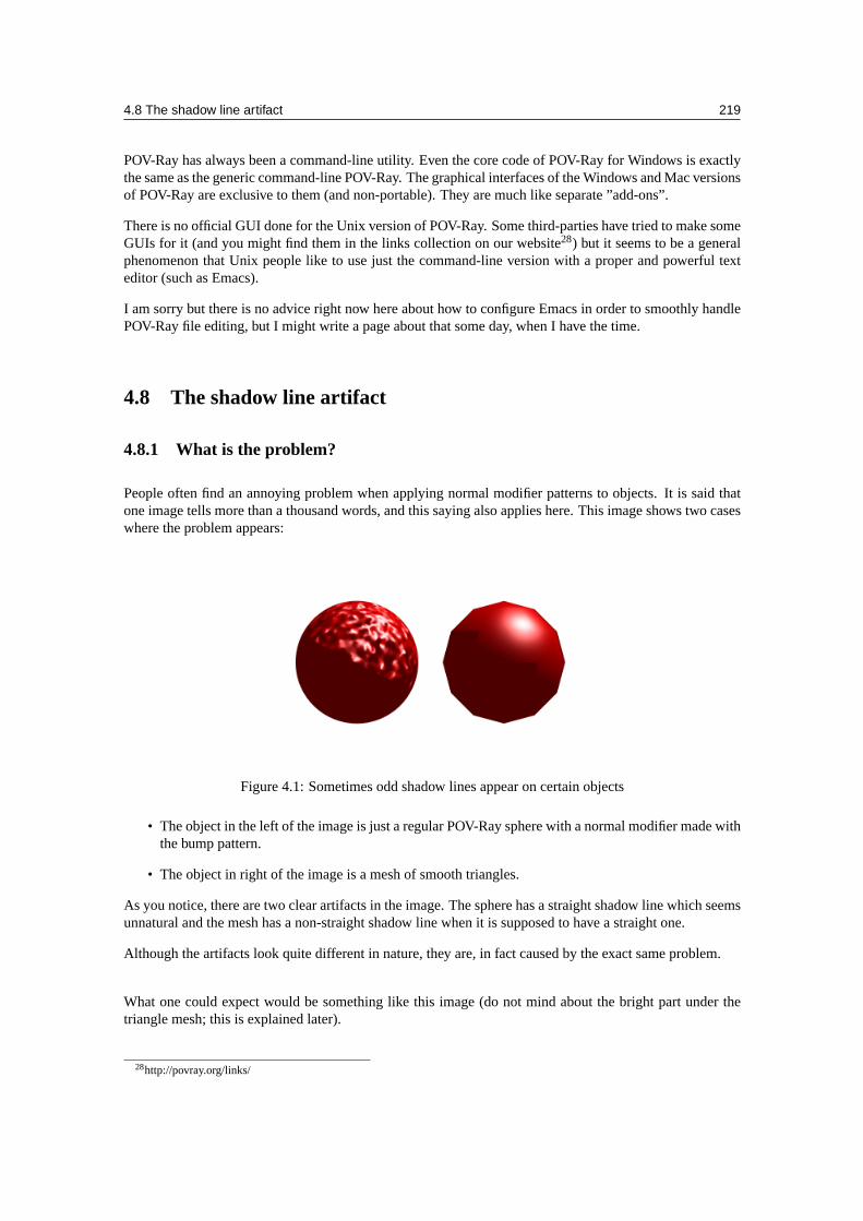
4.8 The shadow line artifact 219
POV-Ray has always been a command-line utility. Even the core code of POV-Ray for Windows is exactlythe same as the generic command-line POV-Ray. The graphical interfaces of the Windows and Mac versionsof POV-Ray are exclusive to them (and non-portable). They are much like separate ”add-ons”.
There is no official GUI done for the Unix version of POV-Ray. Some third-parties have tried to make someGUIs for it (and you might find them in the links collection on our website28) but it seems to be a generalphenomenon that Unix people like to use just the command-line version with a proper and powerful texteditor (such as Emacs).
I am sorry but there is no advice right now here about how to configure Emacs in order to smoothly handlePOV-Ray file editing, but I might write a page about that some day, when I have the time.
4.8 The shadow line artifact
4.8.1 What is the problem?
People often find an annoying problem when applying normal modifier patterns to objects. It is said thatone image tells more than a thousand words, and this saying also applies here. This image shows two caseswhere the problem appears:
Figure 4.1: Sometimes odd shadow lines appear on certain objects
• The object in the left of the image is just a regular POV-Ray sphere with a normal modifier made withthe bump pattern.
• The object in right of the image is a mesh of smooth triangles.
As you notice, there are two clear artifacts in the image. The sphere has a straight shadow line which seemsunnatural and the mesh has a non-straight shadow line when it is supposed to have a straight one.
Although the artifacts look quite different in nature, they are, in fact caused by the exact same problem.
What one could expect would be something like this image (do not mind about the bright part under thetriangle mesh; this is explained later).
28http://povray.org/links/
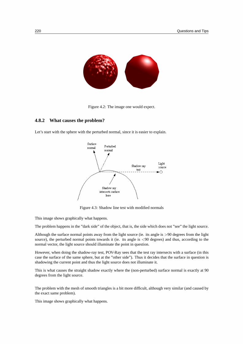
220 Questions and Tips
Figure 4.2: The image one would expect.
4.8.2 What causes the problem?
Let’s start with the sphere with the perturbed normal, since it is easier to explain.
Figure 4.3: Shadow line test with modified normals
This image shows graphically what happens.
The problem happens in the ”dark side” of the object, that is, the side which does not ”see” the light source.
Although the surface normal points away from the light source (ie. its angle is>90 degrees from the lightsource), the perturbed normal points towards it (ie. its angle is<90 degrees) and thus, according to thenormal vector, the light source should illuminate the point in question.
However, when doing the shadow-ray test, POV-Ray sees that the test ray intersects with a surface (in thiscase the surface of the same sphere, but at the ”other side”). Thus it decides that the surface in question isshadowing the current point and thus the light source does not illuminate it.
This is what causes the straight shadow exactly where the (non-perturbed) surface normal is exactly at 90degrees from the light source.
The problem with the mesh of smooth triangles is a bit more difficult, although very similar (and caused bythe exact same problem).
This image shows graphically what happens.
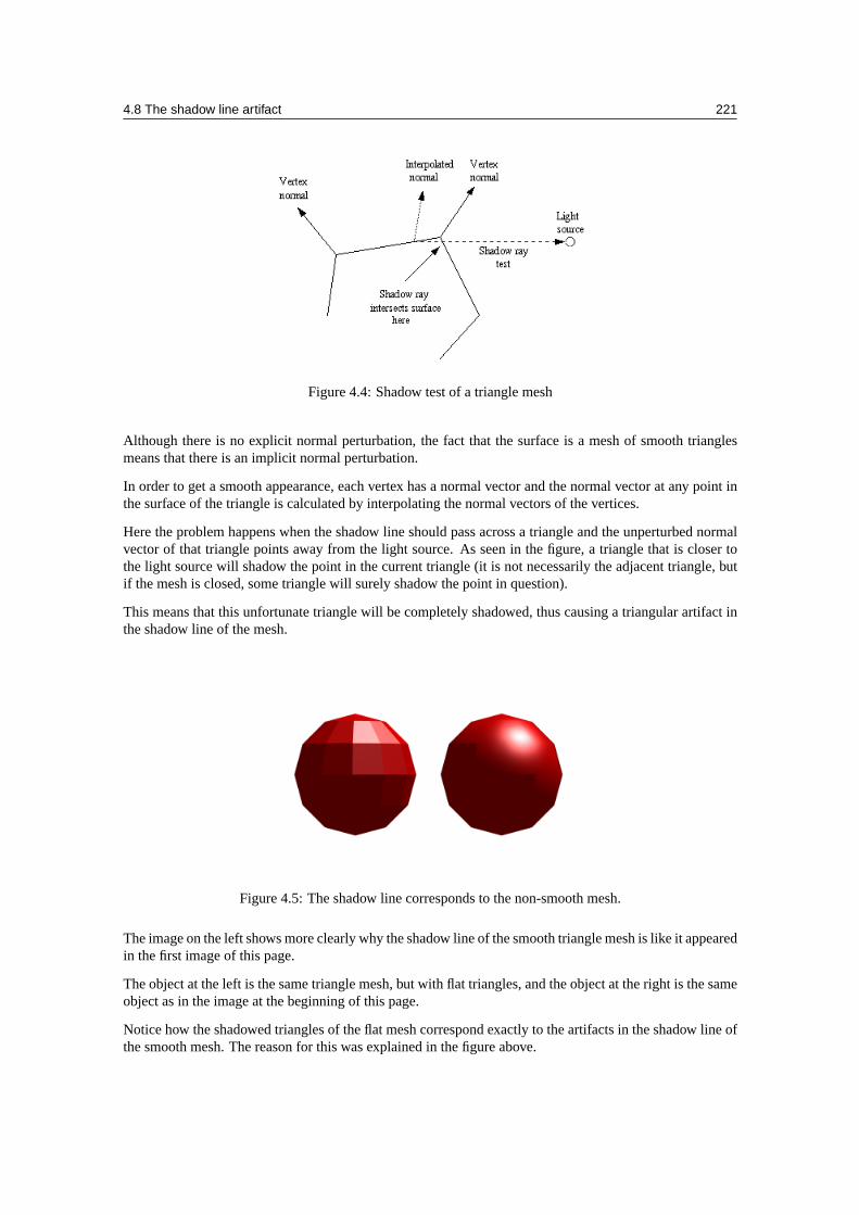
4.8 The shadow line artifact 221
Figure 4.4: Shadow test of a triangle mesh
Although there is no explicit normal perturbation, the fact that the surface is a mesh of smooth trianglesmeans that there is an implicit normal perturbation.
In order to get a smooth appearance, each vertex has a normal vector and the normal vector at any point inthe surface of the triangle is calculated by interpolating the normal vectors of the vertices.
Here the problem happens when the shadow line should pass across a triangle and the unperturbed normalvector of that triangle points away from the light source. As seen in the figure, a triangle that is closer tothe light source will shadow the point in the current triangle (it is not necessarily the adjacent triangle, butif the mesh is closed, some triangle will surely shadow the point in question).
This means that this unfortunate triangle will be completely shadowed, thus causing a triangular artifact inthe shadow line of the mesh.
Figure 4.5: The shadow line corresponds to the non-smooth mesh.
The image on the left shows more clearly why the shadow line of the smooth triangle mesh is like it appearedin the first image of this page.
The object at the left is the same triangle mesh, but with flat triangles, and the object at the right is the sameobject as in the image at the beginning of this page.
Notice how the shadowed triangles of the flat mesh correspond exactly to the artifacts in the shadow line ofthe smooth mesh. The reason for this was explained in the figure above.
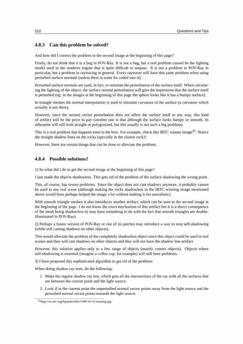
222 Questions and Tips
4.8.3 Can this problem be solved?
And how did I correct the problem in the second image at the beginning of this page?
Firstly, do not think that it is a bug in POV-Ray. It is not a bug, but a real problem caused be the lightingmodel used in the renderer engine that is quite difficult to surpass. It is not a problem in POV-Ray inparticular, but a problem in raytracing in general. Every raytracer will have this same problem when usingperturbed surface normals (unless there is some fix coded into it).
Perturbed surface normals are used, in fact, to simulate the perturbation of the surface itself. When calculat-ing the lighting of the object, the surface normal perturbation will give the impression that the surface itselfis perturbed (eg. in the images at the beginning of this page the sphere looks like it has a bumpy surface).
In triangle meshes the normal interpolation is used to simulate curvature of the surface (a curvature whichactually is not there).
However, since the normal vector perturbation does not affect the surface itself in any way, this kindof artifact will be the price to pay (another one is that although the surface looks bumpy or smooth, itssilhouette will still look straight or polygonized, but this usually is not such a big problem).
This is a real problem that happens even to the best. For example, check this IRTC winner image29. Noticethe straight shadow lines on the rocks (specially in the closest rock)?
However, there are certain things that can be done to alleviate the problem.
4.8.4 Possible solutions?
1) So what did I do to get the second image at the beginning of this page?
I just made the objects shadowless. This gets rid of the problem of the surface shadowing the wrong point.
This, of course, has severe problems. Since the object does not cast shadows anymore, it probably cannotbe used in any real scene (although making the rocks shadowless in the IRTC winning image mentionedabove would have perhaps helped the image a lot without making it too unrealistic).
With smooth triangle meshes it also introduces another artifact, which can be seen in the second image atthe beginning of the page. I do not know the exact mechanism of this artifact but it is a direct consequenceof the mesh being shadowless (it may have something to do with the fact that smooth triangles are double-illuminated in POV-Ray).
2) Perhaps a future version of POV-Ray or one of its patches may introduce a way to stop self-shadowing(while still casting shadows on other objects).
This would alleviate the problem of the completely shadowless object since this object could be used in realscenes and they will cast shadows on other objects and they will not have the shadow line artifact.
However, this solution applies only to a few range of objects (mainly convex objects). Objects whereself-shadowing is essential (imagine a coffee cup, for example) will still have problems.
3) I have proposed this sophisticated algorithm to get rid of the problem:
When doing shadow ray tests, do the following:
1. Make the regular shadow ray test, which gets all the intersections of the ray with all the surfaces thatare between the current point and the light source.
2. Look if in the current point the unperturbed normal vector points away from the light source and theperturbed normal vector points towards the light source.
29http://oz.irtc.org/ftp/pub/stills/1998-10-31/running.jpg
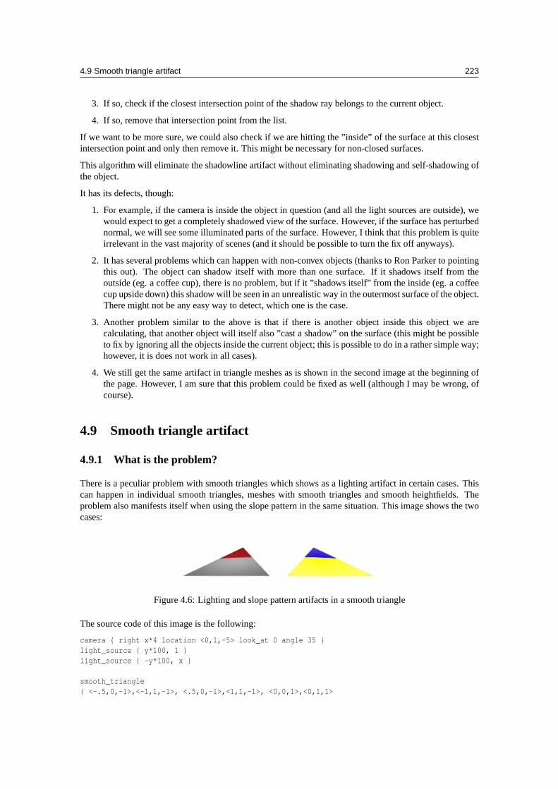
4.9 Smooth triangle artifact 223
3. If so, check if the closest intersection point of the shadow ray belongs to the current object.
4. If so, remove that intersection point from the list.
If we want to be more sure, we could also check if we are hitting the ”inside” of the surface at this closestintersection point and only then remove it. This might be necessary for non-closed surfaces.
This algorithm will eliminate the shadowline artifact without eliminating shadowing and self-shadowing ofthe object.
It has its defects, though:
1. For example, if the camera is inside the object in question (and all the light sources are outside), wewould expect to get a completely shadowed view of the surface. However, if the surface has perturbednormal, we will see some illuminated parts of the surface. However, I think that this problem is quiteirrelevant in the vast majority of scenes (and it should be possible to turn the fix off anyways).
2. It has several problems which can happen with non-convex objects (thanks to Ron Parker to pointingthis out). The object can shadow itself with more than one surface. If it shadows itself from theoutside (eg. a coffee cup), there is no problem, but if it ”shadows itself” from the inside (eg. a coffeecup upside down) this shadow will be seen in an unrealistic way in the outermost surface of the object.There might not be any easy way to detect, which one is the case.
3. Another problem similar to the above is that if there is another object inside this object we arecalculating, that another object will itself also ”cast a shadow” on the surface (this might be possibleto fix by ignoring all the objects inside the current object; this is possible to do in a rather simple way;however, it is does not work in all cases).
4. We still get the same artifact in triangle meshes as is shown in the second image at the beginning ofthe page. However, I am sure that this problem could be fixed as well (although I may be wrong, ofcourse).
4.9 Smooth triangle artifact
4.9.1 What is the problem?
There is a peculiar problem with smooth triangles which shows as a lighting artifact in certain cases. Thiscan happen in individual smooth triangles, meshes with smooth triangles and smooth heightfields. Theproblem also manifests itself when using the slope pattern in the same situation. This image shows the twocases:
Figure 4.6: Lighting and slope pattern artifacts in a smooth triangle
The source code of this image is the following:
camera { right x*4 location <0,1,-5> look_at 0 angle 35 }light_source { y*100, 1 }light_source { -y*100, x }
smooth_triangle{ <-.5,0,-1>,<-1,1,-1>, <.5,0,-1>,<1,1,-1>, <0,0,1>,<0,1,1>
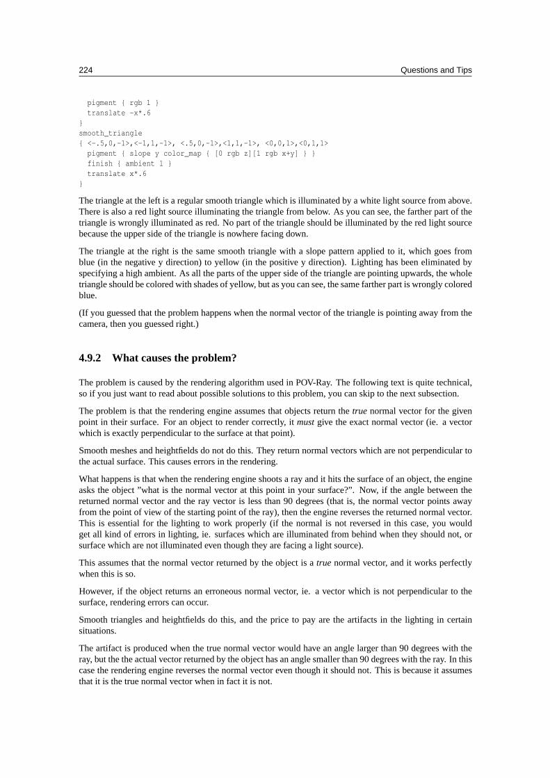
224 Questions and Tips
pigment { rgb 1 }translate -x*.6
}smooth_triangle{ <-.5,0,-1>,<-1,1,-1>, <.5,0,-1>,<1,1,-1>, <0,0,1>,<0,1,1>
pigment { slope y color_map { [0 rgb z][1 rgb x+y] } }finish { ambient 1 }translate x*.6
}
The triangle at the left is a regular smooth triangle which is illuminated by a white light source from above.There is also a red light source illuminating the triangle from below. As you can see, the farther part of thetriangle is wrongly illuminated as red. No part of the triangle should be illuminated by the red light sourcebecause the upper side of the triangle is nowhere facing down.
The triangle at the right is the same smooth triangle with a slope pattern applied to it, which goes fromblue (in the negative y direction) to yellow (in the positive y direction). Lighting has been eliminated byspecifying a high ambient. As all the parts of the upper side of the triangle are pointing upwards, the wholetriangle should be colored with shades of yellow, but as you can see, the same farther part is wrongly coloredblue.
(If you guessed that the problem happens when the normal vector of the triangle is pointing away from thecamera, then you guessed right.)
4.9.2 What causes the problem?
The problem is caused by the rendering algorithm used in POV-Ray. The following text is quite technical,so if you just want to read about possible solutions to this problem, you can skip to the next subsection.
The problem is that the rendering engine assumes that objects return thetrue normal vector for the givenpoint in their surface. For an object to render correctly, itmustgive the exact normal vector (ie. a vectorwhich is exactly perpendicular to the surface at that point).
Smooth meshes and heightfields do not do this. They return normal vectors which are not perpendicular tothe actual surface. This causes errors in the rendering.
What happens is that when the rendering engine shoots a ray and it hits the surface of an object, the engineasks the object ”what is the normal vector at this point in your surface?”. Now, if the angle between thereturned normal vector and the ray vector is less than 90 degrees (that is, the normal vector points awayfrom the point of view of the starting point of the ray), then the engine reverses the returned normal vector.This is essential for the lighting to work properly (if the normal is not reversed in this case, you wouldget all kind of errors in lighting, ie. surfaces which are illuminated from behind when they should not, orsurface which are not illuminated even though they are facing a light source).
This assumes that the normal vector returned by the object is atrue normal vector, and it works perfectlywhen this is so.
However, if the object returns an erroneous normal vector, ie. a vector which is not perpendicular to thesurface, rendering errors can occur.
Smooth triangles and heightfields do this, and the price to pay are the artifacts in the lighting in certainsituations.
The artifact is produced when the true normal vector would have an angle larger than 90 degrees with theray, but the the actual vector returned by the object has an angle smaller than 90 degrees with the ray. In thiscase the rendering engine reverses the normal vector even though it should not. This is because it assumesthat it is the true normal vector when in fact it is not.
4.9 Smooth triangle artifact 225
This problem could be solved by making the decision of inverting the returned normal vector according tothe true normal vector of the surface instead of the returned vector. However, due to the internal imple-mentation of the rendering engine in the current POV-Ray 3.5, doing this is not trivial. It may be fixed inPOV-Ray 4.0, where the rendering engine will be written again and this kind of things can be taken intoaccount from the very beginning.
4.9.3 Can this problem be solved?
You can get rid of the lighting artifact by applyingdouble illuminate to the object in question. When asurface is double illuminated, it does not matter which way its normal points - it will always be illuminatedregardless of which side the light source is. Of course it should not matter that the object is now illuminatedfrom both sides. If this is a problem, then the problem is not easily solvable.
Note that in the example given at the beginning of this section this solution does not work: It wouldilluminate the whole triangle with both light sources! However, this solution works well with closed trianglemeshes, where the inner side of the mesh is shadowed by the mesh itself. However, if you are usingno -
shadow in the object (for example to get rid of shadow line artifacts), new problems can arise in the lighting(such as bright parts in places where there should not be any; these are all cause by this same problem).
The slope pattern is more problematic and there is no generic solution which will work in all cases. Fortu-nately the most common use of the slope pattern is in heightfields, and there a solution is possible:
If you are having this problem in a smooth heightfield, the solution is to mirror the colormap (or whatevermap you are using) around 0.5. This way it does not matter if the normal is reversed. That is, if you hadsomething like this in a heightfield:
slope y color_map{ [0.50 rgb <.5,.5,.5>] // rock
[0.75 rgb <.8,.4,.1>] // ground[1.00 rgb <.4,1,.4>] // grass
}
you simply have to mirror the map around 0.5, ie. add the values from 0 to 0.5 in reverse order:
slope y color_map{ [0.00 rgb <.4,1,.4>] // grass
[0.25 rgb <.8,.4,.1>] // ground[0.50 rgb <.5,.5,.5>] // rock[0.75 rgb <.8,.4,.1>] // ground[1.00 rgb <.4,1,.4>] // grass
}
Besides this you should, of course, applydouble illuminate to the heightfield in order to get the properlighting.

226 Questions and Tips
Chapter 5
Appendices
5.1 POV-Ray User License
POV-Ray License AgreementGENERAL LICENSE AGREEMENTFOR PERSONAL USEPersistence of Vision Ray Tracer™(POV-Ray™)Version 3.6 Licenseand Terms & Conditions of Useversion of 7 June 2004(also known as POVLEGAL.DOC)
Please read through the terms and conditions of this license carefully. This license is a binding legalagreement between you, the ’User’ (an individual or single entity) and Persistence of Vision RaytracerPty. Ltd. ACN 105 891 870 (herein also referred to as the ”Company”), a company incorporated in the stateof Victoria, Australia, for the product known as the ”Persistence of Vision Ray Tracer™”, also referred toherein as ”POV-Ray™”.
YOUR ATTENTION IS PARTICULARLY DRAWN TO THE DISCLAIMER OF WARRANTY ANDNO LIABILITY AND INDEMNITY PROVISIONS. TO USE THE PERSISTENCE OF VISION RAYTRACER (”POV-RAY”) YOU MUST AGREE TO BE BOUND BY THE TERMS AND CONDITIONSSET OUT IN THIS DOCUMENT. IF YOU DO NOT AGREE TO ALL THE TERMS AND CONDI-TIONS OF USE OF POV-RAY SET OUT IN THIS LICENSE AGREEMENT, OR IF SUCH TERMSAND CONDITIONS ARE NOT BINDING ON YOU IN YOUR JURISDICTION, THEN YOU MAYNOT USE POV-RAY IN ANY MANNER. THIS GENERAL LICENSE AGREEMENT MUST ACCOM-PANY ALL POV-RAY FILES WHETHER IN THEIR OFFICIAL OR CUSTOM VERSION FORM. ITMAY NOT BE REMOVED OR MODIFIED. THIS GENERAL LICENSE AGREEMENT GOVERNSTHE USE OF POV-RAY WORLDWIDE. THIS DOCUMENT SUPERSEDES AND REPLACES ALLPREVIOUS GENERAL LICENSES.
INTRODUCTION
This document pertains to the use of the Persistence of Vision Ray Tracer™(also known as POV-Ray™). Itapplies to all POV-Ray program source files, executable (binary) files, scene files, documentation files, helpfiles, bitmaps and other POV-Ray files contained in official Company archives, whether in full or any partthereof, and are herein referred to as the ”Software”. The Company reserves the right to revise these rulesin future versions and to make additional rules to address new circumstances at any time. Such rules, when
228 Appendices
made, will be posted in a revised license file, the latest version of which is available from the Companywebsite at http://www.povray.org/povlegal.html .
USAGE PROVISIONS
Subject to the terms and conditions of this agreement, permission is granted to the User to use the Softwareand its associated files to create and render images. The creator of a scene file retains all rights to anyscene files they create, and any images generated by the Software from them. Subject to the other termsof this license, the User is permitted to use the Software in a profit-making enterprise, provided such profitarises primarily from use of the Software and not from distribution of the Software or a work including theSoftware in whole or part.
Please refer to http://www.povray.org/povlegal.html for licenses covering distribution of the Software andworks including the Software.
The User is also granted the right to use the scene files, fonts, bitmaps, and include files distributed in theINCLUDE and SCENES\INCDEMO sub- directories of the Software in their own scenes. Such permissiondoes not extend to any other files in the SCENES directory or its sub-directories. The SCENES files arefor the User’s enjoyment and education but may not be the basis of any derivative works unless the file inquestion explicitly grants permission to do such.
This licence does not grant any right of re-distribution or use in any manner other than the above. TheCompany has separate license documents that apply to other uses (such as re-distribution via the internet oron CD); please visit http://www.povray.org/povlegal.html for links to these. In particular you are advisedthat the sale, lease, or rental of the Software in any form without written authority from the Company isexplicitly prohibited.
COPYRIGHT
Copyright ©1991-2003, Persistence of Vision Team.Copyright ©2003-2004, Persistence of Vision Raytracer Pty. Ltd.Windows version Copyright ©1996-2003, Christopher Cason.
Copyright subsists in this Software which is protected by Australian and international copyright laws. TheSoftware is NOT PUBLIC DOMAIN.
Nothing in this agreement shall give you any rights in respect of the intellectual property of the Companyand you acknowledge that you do not acquire any rights in respect of such intellectual property rights. Youacknowledge that the Software is the valuable intellectual property of the Company and that if you use,modify or distribute the Software for unauthorized purposes or in an unauthorized manner (or cause orallow the forgoing to occur), you will be liable to the Company for any damages it may suffer (and whichyou acknowledge it may suffer) as well as statutory damages to the maximum extent permitted by law andalso that you may be liable to criminal prosecution. You indemnify the Company and the authors of theSoftware for every single consequence flowing from the aforementioned events.
DISCLAIMER OF WARRANTY
This Software is provided on an ”AS IS” basis, without warranty of any kind, express or implied, includingwithout limitation, any implied warranties of merchantability, fitness for a particular purpose and non-infringement of intellectual property of any third party. This Software has inherent limitations includingdesign faults and programming bugs. The entire risk as to the quality and performance of the Software isborne by you, and it is your responsibility to ensure that it does what you require it to do prior to using itfor any purpose (other than testing it), and prior to distributing it in any fashion. Should the Software provedefective, you agree that you alone assume the entire cost resulting in any way from such defect.
This disclaimer of warranty constitutes an essential and material term of this agreement. If you do not orcannot accept this, or if it is unenforceable in your jurisdiction, then you may not use the Software in anymanner.
5.1 POV-Ray User License 229
NO LIABILITY
When you use the Software you acknowledge and accept that you do so at your sole risk. You agreethat under no circumstances shall you have any claim against the Company or anyone associated directly orindirectly with the Company whether as employee, subcontractor, agent, representative, consultant, licenseeor otherwise (”Company Associates”) for any loss, damages, harm, injury, expense, work stoppage, loss ofbusiness information, business interruption, computer failure or malfunction which may be suffered byyou or by any third party from any cause whatsoever, howsoever arising, in connection with your use ordistribution of the Software even where the Company were aware, or ought to have been aware, of thepotential of such loss. Damages referred to above shall include direct, indirect, general, special, incidental,punitive and/or consequential.
This disclaimer of liability constitutes an essential and material term of this agreement. If you do not orcannot accept this, or if it is unenforceable in your jurisdiction, then you may not use the Software.
INDEMNITY
You indemnify the Company and Company Associates and hold them harmless against any claims whichmay arise from any loss, damages, harm, injury, expense, work stoppage, loss of business information,business interruption, computer failure or malfunction, which may be suffered by you or any other partywhatsoever as a consequence of any act or omission of the Company and/or Company Associates, whethernegligent or not, arising out of your use and/or distribution of the Software, or from any other causewhatsoever, howsoever arising, in connection with the Software. These provisions are binding on yourestate, heirs, executors, legal successors, administrators, parents and/or guardians.
This indemnification constitutes an essential and material term of this agreement. If you do not or cannotaccept this, or if it is unenforceable in your jurisdiction, then you may not use the Software.
HIGH RISK ACTIVITIES
This Software and the output produced by this Software is not fault-tolerant and is not designed, manu-factured or intended for use as on-line control equipment in hazardous environments requiring fail-safeperformance, in which the failure of the Software could lead or directly or indirectly to death, personalinjury, or severe physical or environmental damage (”High Risk Activities”). The Company specificallydisclaims any express or implied warranty of fitness for High Risk Activities and explicitly prohibits theuse of the Software for such purposes.
MISCELLANEOUS
This Agreement constitutes the complete agreement concerning this license. Any changes to this agreementmust be in writing and may take the form of notifications by the Company to you, or through postingnotifications on the Company website. THE USE OF THIS SOFTWARE BY ANY PERSON OR ENTITYIS EXPRESSLY MADE CONDITIONAL ON THEIR ACCEPTANCE OF THE TERMS SET FORTHHEREIN.
Except where explicitly stated otherwise herein, if any provision of this Agreement is found to be invalidor unenforceable, the invalidity or unenforceability of such provision shall not affect the other provisionsof this agreement, and all provisions not affected by such invalidity or unenforceability shall remain in fullforce and effect. In such cases you agree to attempt to substitute for each invalid or unenforceable provisiona valid or enforceable provision which achieves to the greatest extent possible, the objectives and intentionof the invalid or unenforceable provision. The validity and interpretation of this agreement will be governedby the laws of Australia in the state of Victoria (except for conflict of law provisions).
CONTACT INFORMATION
License inquiries can be made via email; please use the following address (but see below prior to emailing):
team-coord-[three-letter month]-[four-digit year]@povray.org
230 Appendices
for example,[email protected] should be used if at the time you send the email it is themonth of June 2004. The changing email addresses are necessary to combat spam and email viruses. Oldemail addresses may be deleted at our discretion.
Note that the above address may change for reasons other than that given above; please check the versionof this document on the WWW at http://www.povray.org/povlegal.html for the current address. Note thatyour inability or failure to contact us for any reason is not an excuse for violating this licence.
Do NOT send any attachments of any sort other than by prior arrangement. EMAIL MESSAGES INCLUD-ING ATTACHMENTS WILL BE DELETED UNREAD.
The following postal address is only for official license business. Please note that it is preferred that initialqueries about licensing be made via email; postal mail should only be used when email is not possible, orwhen written documents are being exchanged by prior arrangement.
Persistence of Vision Raytracer Pty. Ltd.PO Box 407Williamstown,Victoria 3016Australia
5.2 Citing POV-Ray in Academic Publications
To reference POV-Ray (e.g. in academic papers), you may use one of the below:
Persistence of Vision Pty. Ltd. (2004)Persistence of Vision Raytracer (Version 3.6)[Computer software].
Retrieved from http://www.povray.org/download/
or
Persistence of Vision Pty. Ltd. (2004).Persistence of Vision (TM) Raytracer.Persistence of Vision Pty. Ltd., Williamstown, Victoria, Australia.http://www.povray.org/
5.3 The POV-Team
Following is a list in alphabetic order of all people who have ever worked on the POV-Ray Team or whohave made a note-worthy contribution.
Current POV-Team Members
Chris CasonMember 1993-, Team leader 1999-, windows version author, other contributions
Nicolas Calimet3.6 UNIX development
Dale C. BrodinAlpha & Beta tester, forum support
Alexander EnzmannPOV-Ray 1.0/2.0/3.0 developer
5.3 The POV-Team 231
Thorsten FrohlichMac developer
Christoph Hormann3.6 UNIX development
Alan KongAlpha & Beta tester, forum support
Nathan KoppPhotons, u/v mapping, other contributions.
Lutz KretzschmarMoray author, MS-DOS 24-bit VGA, part of the anti-aliasing code
Ron ParkerCore code, jack-of-all-trades
Anton RavesAlpha & Beta tester, Mac contributor
Erkki SondergaardAlpha & Beta tester, 3.0 Scene files
Past POV-Team Members and other Contributors
Claire AmundsenTutorials for the POV-Ray User Guide
Steve AngerPOV-Ray 2.0/3.0 developer
Randy AntlerMS-Dos display code enhancements
John BailyRLE targa code
Eric BarishGround fog code
Thomas Baier3.1 team member, tester
Dieter BayerWrote sor, lathe, prism, media and many other features
Anthony BennettScene files, documentation
Kendall BennettPMODE library support, paletted display code in Windows version
Steve BennettGIF support
Thomas BilyImplicit and parametric surfaces
Eric Brownno image, noreflection, orient and circular arealight
Matthew Corey Brown
232 Appendices
pigment function, warps
David BuckOriginal author of DKBTrace, POV-Ray 1.0 developer
Edward CoffeyFadecolor
Aaron CollinsCo-author of DKBTrace 2.12, POV-Ray 1.0 developer
Chris DaileyPOV-Ray 3.0 developer
Steve DemlowPOV-Ray 3.0 developer
Andreas DilgerFormer Unix coordinator, Linux developer, PNG support
Joris van Drunen LittelMac beta tester
Dan FarmerPOV-Ray 1.0/2.0/3.0 developer, author of many features, sample scenes, and textures
Daniel FennerSplines
Hans-Detlev FinkSlope pattern
Charles FusnerBlob, lathe and prism tutorial tutorials for the POV-Ray User Guide
Mark GordonUnix developer
Jerome GrimbertMapping warps
David HarrMac balloon help and palette code
Michael HazelgroveScene files
Jimmy HoeksOriginal Help file for v3.0 Windows user interface
Christoph HormannScene & include files, documentation, insert menu
Chris HuffObject pattern, Interior texture, inverse transform
Bob HughesScene and include files, insert menu
Ingo JanssenScene & include files, documentation
Mike Hough
5.3 The POV-Team 233
Spherical camera, Media method 2, uvmapping for bicubicpatch
Rune S. JohansenScene & include files, documentation
Greg M. JohnsonScene files
Terry KanakisCamera fix
Kari KivisaloGround fog code
Tor Olav KristensenScene files
Jochen LippertSpheresweep
Charles MarslettMS-Dos display code
Pascal MassiminoFractal objects
Jim McElhineyPOV-Ray 3.0 developer
Robert A. MickelsenArtist, 3.0 docs contributor
Mike MillerArtist, scene files, stones.inc
Fabien MosenScene & include files
Douglas MuirBump maps, height fields
Joel NewkirkFormer Amiga developer
Juha NieminenFractal patterns
Jim Nitchals1
Mac version, scene files (Jim - famous also for his anti-spam crusades - passed away on 5 June19982 but his contributions to POV-Ray and responsible use of the internet will not be forgotten)
Paul NovakTexture contributions
Wolfgang OrtmannSplines
Dave ParkAmiga support, AGA video code
Redaelli Paolo1http://www.igorlabs.com/jim/jim.html2http://www.wired.com/news/culture/0,1284,12832,00.html
234 Appendices
Former Amiga developer
David PayneRLE targa code
Ansgar PhilippsenSmooth color triangle
Bill PulverTime code
Dan Richardson3.0 Docs
Tim RowleyPPM and Windows-specific BMP image format support
Eduard SchwanFormer Mac version coordinator, mosaic preview, docs
Daniel SkardaImplicit and parametric surfaces
Robert SkinnerNoise functions
Yvo & Rene SmellenberghClock & Imagesize keywords
Ryoichi SuzukiIsosurfaces
Zsolt SzalavariHalo code which was later turned into media
Scott TaylorLeopard and onion textures
Gilles TranScene files
John VanSickleCells pattern
Mark WagnerSplines
Timothy WegnerFractal objects, PNG support
Drew WellsPOV-Ray 1.0 developer, POV-Ray 1.0 team coordinator
Daren Scot WilsonDispersion
Chris YoungTeam leader 1992-1999, parser code, other contributions too numerous to list here
5.3 The POV-Team 235
5.3.1 Contacting the Authors
The POV-Team is a collection of volunteer programmers, designers, animators and artists meeting via theinternet at http://www.povray.org/. The POV-Team’s goal is to create freely distributable, high qualityrendering and animation software written in C that can be easily ported to many different computers. If youhave any questions about POV-Ray, please visit our web site for the latest contact information, or see theonline version of POVLEGAL3 for the current team coordinators address (this changes from time to timewhenever too many email spammers harvest the address).
If you have a question regarding commercial use or distribution of POV-Ray, please contact Chris Cason,the development team coordinator, via the above method. Please do not email us directly for technicalsupport; we no longer give support via email as too many people abused the privilege.
See our web site4 and particularly our news server5 for online peer support. The news server has a moder-ated bug reporting newsgroup; please however discuss the issue in the povray.general6 newsgroup prior tolodging a bug report as we may already know of the issue (or it might not even be a bug). Also, there areseveral FAQ’s on the POV web site, and in general the folks in the newsgroups think rather poorly of userswho post complaints without reading the FAQ’s first.
Finally, there is also a dedicated Technical Assistance Group consisting of a number of trusted, experiencedPOV-Ray users.
5.3.2 The TAG
Established by the POV-Team in late 1999, the TAG (Technical Assistance Group) is made up of selectedmembers of the POV-Ray user community. The purpose of the TAG is to aid the POV-Team in supportingusers of POV-Ray around the world, using the collective knowledge of the group to answer users’ POV-Rayquestions and to bring POV-Ray related matters to the attention of the POV-Team as required.
With their range of experiences in particular areas of computing and graphics, TAG members will alwaystry to provide an answer to users’ POV-Ray questions as best they can. If members of the TAG feel aquestion or suggestion merits the attention of the POV-Team, they will redirect queries to the appropriatemembers of the Team for consideration.
TAG members are not members of the POV-Team. But they are, however, an official conduit between usand the outside world. They have direct access to all members of the POV-Team. They have the right tospeak on our behalf on the POV-Ray news server and on any official mailing lists that we set up for thispurpose. Not everything they say will be official; only when they sign it as such. They can still act as’themselves’ and have their own opinions at all other times.
The TAG has its own website7.
Technical Assistance Group Members
Chris ColefaxEmail: chris.colefax [at] tag.povray.org
Chris HuffEmail: chris.huff [at] tag.povray.org
Ingo JanssenEmail: ingo [at] tag.povray.org
3http://www.povray.org/povlegal.html4http://www.povray.org/5http://www.povray.org/groups.html6news://news.povray.org/povray.general7http://tag.povray.org/

236 Appendices
Juha NieminenEmail: warp [at] tag.povray.org
Peter PopovEmail: peter.popov [at] tag.povray.org
Margus RamstEmail: margus.ramst [at] tag.povray.org
Gilles TranEmail: gilles.tran [at] tag.povray.org
Ken TylerEmail: ken.tyler [at] tag.povray.org
5.3.3 POV-Ray 3.6 Development
Main 3.6 developers:
Chris Cason
Thorsten Frohlich
Nathan Kopp
Contributors of patches in POV-Ray 3.6
Nicolas CalimetUNIX development
Christoph HormannUNIX development
Wlodzimierz ’ABX’ SkibaVarious fixes, uv-mapping for parametric and torus
Massimo ValentiniVarious fixes
5.4 What to do if you don’t have POV-Ray
This documentation assumes you already have POV-Ray installed and running however the POV-Team doesdistribute this file by itself in various formats including online on the internet. If you do not have POV-Rayor are not sure you have the official version or the latest version, then the following sections will tell youwhat to get and where to get it.
5.4.1 Which Version of POV-Ray should you use?
POV-Ray can be used under Windows 9x/NT/2000, Apple Power PC, x86 Linux, UNIX and other plat-forms. The latest versions of the necessary files are available on our web site8 and through various CDdistributions. See section ”Where to Find POV-Ray Files” for more info. Dos, Windows 3.1, Windows forWorkgroups, SunOS and Amiga are no longer supported. If your platform is not supported and you areproficient in compiling source code programs written in C/C++, then you may like to retrieve the source forPOV-Ray from our website and attempt to built it yourself. Note that the POV-Team provides absolutely
8http://www.povray.org/
5.4 What to do if you don’t have POV-Ray 237
no support for building POV-Ray from the source code, especially on platforms that we do not officiallysupport.
Microsoft Windows 9x/NT/2000/XP
The 32-bit Windows version runs under Windows 95, Windows 98, NT, 2000 and XP or newer. Requiredhardware and software: Minimum - 486/100 with 32mb RAM and Windows 95. Disk space - 20 megabytes.Recommended - Pentium 4 or equivalent with at least 256mb of RAM running Windows 2000 or XP,equipped with an XGA display (or better) running in true color mode.
The forthcoming 64-bit Windows version will initially run under Windows XP 64-bit edition on AMD64-based machines, or those compatibile with them. The recommended configuration has not yet been deter-mined but as a rule of thumb we would suggest at least 256mb RAM (512mb preferred).
Note: accelerated graphics hardware will not improve performance. Nor will MMX or 3D Now. Thesetechnologies are not aimed at raytracing. SSE2-equipped CPU’s (such as the Pentium 4) will enhanceperformance if and only if an SSE2-enabled version of POV-Ray for Windows is installed. If we makesuch a version available it will be provided on our website and FTP server using a different name than thatmentioned below.
Required POV-Ray files: User archive POVWIN36.EXE - a self-extracting archive containing the program,sample scenes, standard include files and documentation.
Optional: The source code is not needed to use POV-Ray. It is provided for the curious and adventurous.POVWIN S.ZIP — The C/C++ source code for POV-Ray for Windows, contains generic parts and Windowsspecific parts. It does not include sample scenes, standard include files and documentation so you shouldalso get the executable archive as well. POV-Ray can only be compiled using C/C++ compilers that create32-bit Windows applications.
We currently support VC++ v7 (v6 willnot work due to compiler issues with certain C++ features), BorlandC++, Open Watcom, MinGW, and DJGPP (BJGPP 2.04 or later), and the Intel C++ Compiler version8. Support for both Intel and Microsoft’s C++ compiler for AMD64 is also in the works and will beforthcoming in a later source code release (once we release an official 64-bit version of POV-Ray forWindows).
Note that no matter which compiler you use, you will need to obtain the HTML Help API toolkit fromMicrosoft’s web site (unless you already have it installed). This toolkit contains header files and librariesrequired to compile POV-Ray for Windows.
Note: while we know for certain that the code will work with VC++ v7 and the Intel compiler v8, the othersmentioned above may need some tweaking since we do not regularly test with them and it is possible somelater code changes may have broken the build.
Linux for Intel x86
The PC-Linux version should run on any GNU/Linux distribution based on the kernel 2.2 series or aboveusing the ELF 32-bit format for executables. The binary is fully static, meaning that it has no externaldependencies to system or third-party libraries. It includes support for two kinds of display: the standardtext-based display and the graphics display using either the X Window System or the SVGA library.
Required hardware and software: An Intel Pentium-compatible CPU (i586 or better) and at least 32 MB ofRAM. About 20 MB of disk space to install the program, its documentation, scenes and standard includefiles. A text editor capable of editing plain ASCII text files. Graphic file viewer capable of viewing imageformats such as PNG, TIFF, PPM or TGA.
238 Appendices
Required POV-Ray files: povlinux-3.6.tgz or povlinux-3.6.tar.gz - archive containing an official binarycombining text, SVGALib and X Window displays. Also contains sample scenes, standard include filesand documentation in HTML and plain ASCII text.
Recommended: Intel Pentium 4 or AMD Athlon XP (faster the better) with 128 MB (text console) / 256MB (X Window running a window manager) or more RAM. A recent GNU/Linux distribution with kernel2.4.x or above running KDE 3.x for full POV-Ray integration in the window manager. Alternatively, SVGAdisplay preferably with VESA interface and high color or true color ability.
Note: accelerated graphics hardware will not improve performance.
Optional: povray-3.6.tgz or povray-3.6.tar.gz - archive containing the generic UNIX/Linux C++ sourcecode of POV-Ray for UNIX. The source code is not needed to use POV-Ray. It is provided for the curiousand adventurous. The archive contains generic Unix parts and Linux specific parts (namely: support forSVGAlib). This package does also include sample scenes, standard include files and documentation. Fordisplaying purposes, the SVGAlib and X11 (X Window) includes and libraries can be used by the sourcecode of POV-Ray for UNIX. See the section related to the generic Unix source code package for furtherdetails.
Apple Macintosh
The Macintosh version runs under Apple’s Mac OS operating system version 8.6 (it may run on 8.1 and8.5 as well, but we do not support POV-Ray 3.6 running on Mac OS 8.1 and 8.5) or newer with CarbonLib1.0.4 or newer installed. Note that we no longer support 68K based Macintosh computers. POV-Ray 3.6requires a Power Macintosh!
A Power Macintosh is any iMac, iBook, Mac G3, Mac G4, Mac G5, Cube, any older Mac with a four digitmodel number (i.e. 5200, 6300, 7200, 8100, 9600) and any third party computer running Mac OS 8.1 orlater. Mac OS X 10.2 or later are supported but for maximum render speed it is not recommended to useMac OS X.
Required hardware and software: Power Macintosh computer with at least 16 MB of free RAM. Mac OS 8.6or newer with CarbonLib 1.0.4 or newer installed CarbonLib 1.0.4. About 20 MB free disk space to installand an additional 5-10 MB free space for your own creations (scenes and images). Graphic file viewer utilitycapable of viewing Mac PICT, GIF and perhaps TGA and PNG formats (the shareware GraphicConverterapplications is good.)
Required POV-Ray files: POVPMAC.SIT or POVPMAC.HQX - a StuffIt archive containing the nativePower Macintosh application, sample scenes, standard include files and documentation.
Recommended: Power Macintosh G3 with 64 MB or more of free RAM. Mac OS 9.0.4 or newer withCarbonLib 1.6 (works with Mac OS 8.6 or newer) to access all features of the Mac frontend. CarbonLib1.6 is available for free download from Apple in the software update section of the Apple website. Colormonitor with millions of colors.
Optional: The source code is not needed to use POV-Ray. It is provided for the curious and adventurous.POV-Ray can be compiled using Metrowerks CodeWarrior Pro 7.2 (for other compilers no project or makefiles are provided). Read the file ”How to compile!” before compiling. There is no other support or helpfor compiling the source code! POVMACS.SIT or POVMACS.HQX - The full C source code for POV-Rayfor Macintosh. Contains generic parts and Macintosh specific parts. It does not include sample scenes,standard include files and documentation so you should also get the executable archive as well.
5.4 What to do if you don’t have POV-Ray 239
Generic Unix
Because Unix runs on a wide variety of hardware and CPUs, the POV-Team cannot provide executableversions for every kind of Unix systems. We distribute a generic, portable C++ source code suitable forrunning on Unix or Unix-like platforms. You will need a recent C++ compiler which follows the ISO C++standard as close as possible, and (optionally) the X11 and/or SVGA include files and libraries (SVGAlibis for GNU/Linux based systems). Although we provide source code for generic Unix systems, we do notprovide technical support on how to compile the program. Support may be obtained from the POV-Ray usercommunity on the dedicated POV-Ray newsgroups (povray.unix at news.povray.org).
Required hardware and software: A UNIX operating system with 32 MB of RAM. A recent C++ compiler,a working make utility and Bourne-compatible shell; see the INSTALL file in the package for details.Graphic file viewer capable of viewing e.g. PNG, TIFF, PPM or TGA formats. A text editor capable ofediting plain ASCII text files.
Required POV-Ray files: povray-3.6.tgz or povray-3.6.tar.gz - the C++ source code of POV-Ray for UNIX.Contains generic parts and UNIX/Linux specific parts. The package includes sample scenes, standardinclude files and documentation in HTML and plain text ASCII format.
Recommended: Math co-processor. 128 MB (text console) / 256 MB (X Window running a windowmanager) or more RAM.
Optional: The X Window System (e.g. XFree86) to be able to display the image while rendering. The XWindow System is available on most UNIX platforms nowadays. On GNU/Linux platforms, the SVGAliblibrary can be an alternative to the X Window System, as it allows to display the rendered image directly onthe console screen.
All Versions
Each executable archive includes full documentation for POV-Ray itself as well as specific instructionsfor using POV-Ray with your type of platform. All versions of the program share the same ray-tracingfeatures like shapes, lighting and textures. In other words, an MS-Dos-PC can create the same picturesas a Cray supercomputer as long as it has enough memory. The user will want to get the executable thatbest matches their computer hardware. In addition to the files listed above, the POV-Team also distributesthe user documentation in two alternate forms. Note this is the same documentation distributed in otherarchives but in a different format. This may be especially useful for MS-Dos or Unix users because theirdocumentation is plain ASCII text only. POVUSER.PDF - Tutorial and Reference documentation in AdobeAcrobat PDF format. Requires Adobe Acrobat Reader available for Windows 3.x, Windows 95/98/NT, Macand some Unix systems. POVHTML.ZIP - Archive containing Tutorial and Reference documentation inHTML for viewing with any internet browser.
See the section ”Where to Find POV-Ray Files” for where to find these files. You can contact those sourcesto find out what the best version is for you and your computer.
5.4.2 Where to Find POV-Ray Files
The latest versions of the POV-Ray software are available from the following sources.
240 Appendices
World Wide Website www.povray.org
The internet home of POV-Ray is reachable on the World Wide Web via the address http://www.povray.org/9 and via ftp as ftp://ftp.povray.org/10. Please stop by often for the latest files, utilities, news and imagesfrom the official POV-Ray internet site. The POV-Team operates its own news server11 on the internet withseveral news groups related to POV-Ray and other interesting programs.
Books, Magazines and CD-ROMs
If you would like to print our documentation, it is available in a number of formats that are designed forprinting. In particular, PDF, postscript, and TeX. See the POV-Ray website for more details.
Unfortunately all English language books on POV-Ray are out of print and there are no plans to reprint them.However there are now several POV-Ray books available in Japanese. Many popular computer magazineshave been authorized to distribute POV-Ray on cover CD’s. From time to time we, the makers of POV-Ray,will ourselves make CDROM’s available, either direct from our website or from authorized distributors.See the our website12 for more information, as that location will always contain the most up-to-date details.
5.5 Suggested Reading
Beside the POV-Ray material mentioned in ”Books, Magazines and CD-ROMs” there are several goodbooks or periodicals that you should be able to locate in your local computer book store or your localuniversity library.
1. ”An Introduction to Ray tracing” Andrew S. Glassner (editor)ISBN 0-12-286160-4; Academic Press; 1989
2. ”Realistic Image Synthesis Using Photon Mapping” Henrik Wann JensenISBN: 1568811470; AK Peters; July 2001
3. ”3D Artist” Newsletter, ”The Only Newsletter about Affordable PC 3D Tools and Techniques”)Publisher: Bill Allen; P.O. Box 4787; Santa Fe, NM 87502-4787; (505) 982-3532
4. ”Image Synthesis: Theory and Practice” Nadia Magnenat-Thalman and Daniel Thalmann;Springer-Verlag; 1987
5. ”The RenderMan Companion” Steve Upstill;Addison Wesley; 1989
6. ”Graphics Gems” Andrew S. Glassner (editor);Academic Press; 1990
7. ”Fundamentals of Interactive Computer Graphics” J. D. Foley and A. Van Dam;ISBN 0-201-14468-9; Addison-Wesley 1983
8. ”Computer Graphics: Principles and Practice (2nd Ed.)” J. D. Foley, A. van Dam, J. F. Hughes;ISBN 0-201-12110-7; Addison-Wesley; 1990
9. ”Computers, Pattern, Chaos, and Beauty” Clifford Pickover;St.Martin’s Press;
9http://www.povray.org/10ftp://ftp.povray.org/11http://www.povray.org/groups.html12http://www.povray.org/

5.5 Suggested Reading 241
10. ”SIGGRAPH Conference Proceedings”;Association for Computing Machinery Special Interest Group on Computer Graphics
11. ”IEEE Computer Graphics and Applications”; The Computer Society;10662, Los Vaqueros Circle; Los Alamitos, CA 90720
The POV-Teamno longer recommendsbooks from CRC Press. Go read Eric’s commentary13 to find outwhy.
13http://mathworld.wolfram.com/ericscommentary.html

242 Appendices
Index
POVLEGAL.DOC, 227
Ambientusing, 114
ambientlighttutorial, 30
Animationclock variable, 160INI file settings for, 164multi-stage, 161not using jitter or crand with, 164
Area Light Sourcethe, 29
Atmospheric Effectsusing, 130
averagetutorial, 121
Backgroundtutorial, 130
bicubic patchtutorial, 60
black spots, 203Blob Constructs
complex, 80box
tutorial, 15Bumpiness
adding, 33
Cameraadding, 13using the, 35
citations, 230Clouds
adding, 133Color List Pigments
using, 107Color Maps, 33Color Patterns
creating, 33color map
tutorial, 33Command-line Options, 41
all versions, 41
conetutorial, 16
Constructive Solid Geometry, 22Coordinate System
understanding, 11crand
in animations, 164CSG
what is, 22cubic spline
tutorial, 54cylinder
tutorial, 16Cylindrical Light Source
the, 29
DifferenceCSG, 24
differencetutorial, 24
Environment variablesPOVINI, 43POVRAYOPT, 43
Fading Light, 32FAQ, 195final clock
ini-option, tutorial, 164final frame
ini-option, tutorial, 164finish
tutorial, 113Focal Blur
using, 35focus, 35Fog
adding, 134adding turbulence, 137constant, 135filtering, 136ground, 138hollow objects, 139setting minimum translucency, 135using multiple layers of, 138
244 INDEX
fogtutorial, 134
frequencytutorial, 108
Ground Fogusing, 138
height fieldtutorial, 81
Highlights, 115Hollow Objects
fog inside, 139
INI filesusing, 42
initial clockini-option, tutorial, 164
initial frameini-option, tutorial, 164
Interference, 117Intersection
CSG, 23intersection
tutorial, 23Irid
using, 117isosurface
tutorial, 83
jitterin animations, 164
keyword:#include, 12
lambdatutorial, 108
lathetutorial, 45
Layered Texturesanother example, 124declaring, 124using, 109working with, 122
Left-Handed coordinate system, 11License, 227Light Fading
using, 32Light Source
assigning an object to, 31the, 26
Light Sourcesspecial, 31
light source
arealight, tutorial, 29cylinder, tutorial, 29defining, 14fadepower, tutorial, 32looks like, tutorial, 31shadowless, tutorial, 31spotlight, tutorial, 28tutorial, 26
List Texturesworking with, 120
materialmaptutor, 127
mediatutorial, 143
MergeCSG, 25
mergetutorial, 25
meshtutorial, 67
Metallicusing, 116
Negative Strengthblob, 80
New Featurescomponent types, 79
Normal Mapsworking with, 119
Normal Modifiersusing, 111
normalmaptutorial, 112using, 119
Normalsblending, 112
Normals and Radiosity, 159
Objectadding texture to, 14describing, 13
Object Lights, 31octaves
tutorial, 108omega
tutorial, 108Options
all versions, 41command-line, 41ini file, 42POVINI environment variable, 43setting, 41
INDEX 245
Pattern Modifiersusing, 108
Patterns, 33phase
tutorial, 163phong
tutorial, 115pigment
tutorial, 106Pigment and Patterns
using, 107Pigment Maps
using, 110working with, 118
pigmentmaptutorial, 110
PitfallsCSG, 26
planetutorial, 16
Pointlight Sourcethe, 26
polytutorial, 97
polygontutorial, 75
POV-Ray Legal Document, 227pov-ray license, 227POVINI environment variable, 43POVLEGAL, 227POVRAYOPT environment variable, 43prism
tutorial, 54
Questions and Tips, 195
Radiositytutorial, 150with conventional lighting, 151without conventional lighting, 155
Radiosity performance considerations, 159Rainbow
increasing translucency of, 141simple, 139the, 139using an arc, 142
rainbowtutorial, 139
Ray-Tracingwhat is, 2
reference, 230Reflection
using, 116
Right-Handed coordinate system, 12
Shadowless Lightsusing, 31
Shapesbasic, 15other, 77polygon based, 67spline based, 45
Skywith a color gradient, 131
Sky Spherethe, 131
sky spheretutorial, 131
sortutorial, 52
Special Textureslimitations of, 129
spheresweeptutorial, 59
Splinenew tricks, 54
Splinesunderstanding the concept of, 47
Spotlight Sourcethe, 28
Standard Include Filesadding, 12
superellipsoidtutorial, 103
Surface Highlightsusing, 115
Surfacesco-incident, 26
Switchescommand-line, 41
Tapering Conic Sweeps, 57text
tutorial, 65Texture Maps
working with, 119Texture Options
advanced, 106simple, 33
texturemaptutorial, 119
Texturespre-defined, 34
The Left-Handed coordinate system, 11Thin-Film Interference, 117Tiles

246 INDEX
what about, 121torus
tutorial, 17Transparent Pigments
using, 109turbulence
tutorial, 108
UnionCSG, 22
uniontutorial, 22
user license, 227
variable ior, 207VFAQ, 195
Related Documents