Introduction to highway engineering

Highway Engineering

Pavement Design

10.1 Introduction to highway engineering

Transportation planning and traffic planning are the initial stages of transportation engineering

pertaining to road transport. Having planned highways, the next stage is the construction of the

highways. The roads have to be constructed in different ground conditions and in different

environments. The conditions and environments pose complex issues in highway construction. In

many countries’s context, these issues are,

Congestion on urban roads

Accidents

Major roads running through built up areas (Cities and townships)

Narrow roads

Structural inadequacy of pavements

Poor geometrical design

Small structures such as bridges

Funding for maintenance and rehabilitation

Funding for expansion and new facilities

Environmental pollution

These issues provide the following challenges to the highway engineer.

(1) Challenges of design, construction, rehabilitation, reconstruction and expansion

(i.) Design and reconstruct using modern technologies

(ii.) Redesign older facilities to meet today’s demands.

(iii.) Secure budget provisions.

(iv.) Adopt cost effective and environmentally sound solutions.

(2) Challenges of safety and environment

(i.) Identify necessary safety requirements of the road system especially, to protect

vulnerable road users.

(ii.) Implement regulations controlling noise, air and water pollution.

10.2 Pavement Design

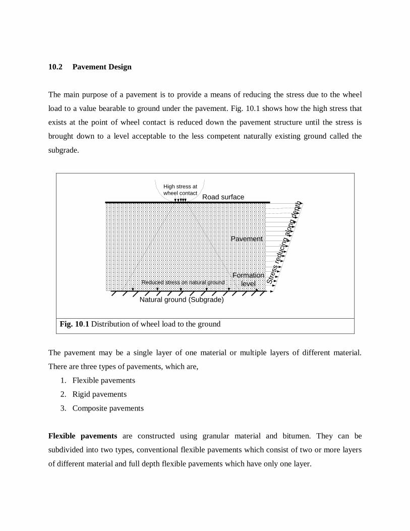
The main purpose of a pavement is to provide a means of reducing the stress due to the wheel

load to a value bearable to ground under the pavement. Fig. 10.1 shows how the high stress that

exists at the point of wheel contact is reduced down the pavement structure until the stress is

brought down to a level acceptable to the less competent naturally existing ground called the

subgrade.

High stress at

wheel contactRoad surface

Reduced stress on natural ground

Natural ground (Subgrade)

Formation

level

Pavement

Str

ess

reducin

g a

long d

epth

Fig. 10.1 Distribution of wheel load to the ground

The pavement may be a single layer of one material or multiple layers of different material.

There are three types of pavements, which are,

1. Flexible pavements

2. Rigid pavements

3. Composite pavements

Flexible pavements are constructed using granular material and bitumen. They can be

subdivided into two types, conventional flexible pavements which consist of two or more layers

of different material and full depth flexible pavements which have only one layer.

Rigid pavements are constructed of Portland cement concrete (PCC)

Composite pavements have a base layer of PCC and a surface layer of hot-mix asphalt. They

have strength of rigid pavements and smooth surface of flexible pavements.

There are two factors which lead to the development of layered flexible pavement construction.

They are

(i.) the stresses from vehicles travelling on the road are highest near the surface

(ii.) a smooth riding surface is necessary to reduce fatigue due to varying stresses on

surface.

Kerb

Backfill

Wearing course

Subgrade

Formation

Roadbase

BasecourseWalkway

Camber

Sub-base

Carriageway

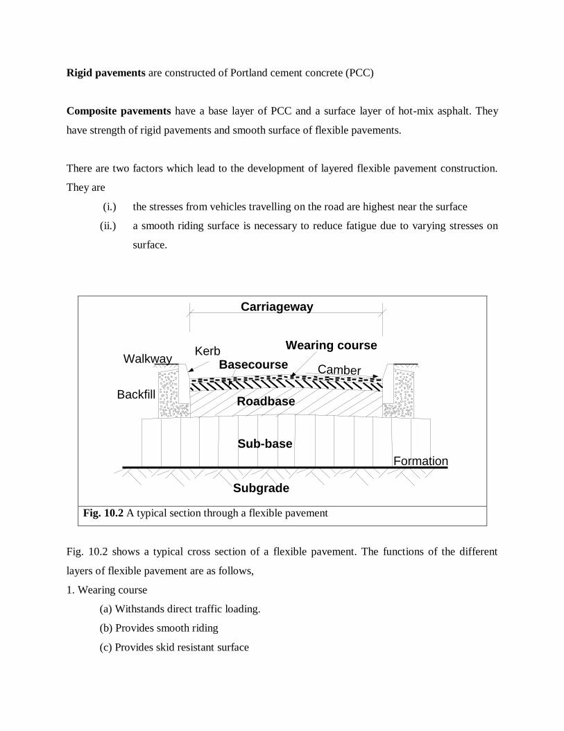
Fig. 10.2 A typical section through a flexible pavement

Fig. 10.2 shows a typical cross section of a flexible pavement. The functions of the different

layers of flexible pavement are as follows,

1. Wearing course

(a) Withstands direct traffic loading.

(b) Provides smooth riding

(c) Provides skid resistant surface

(d) Waterproofs the pavement

2. Basecourse

(a) Supports wearing course

(b) Assists protecting layers below

3. Roadbase

(a) Main load spreading layer of the pavement structure

4. Sub-base

(a) Assists load spreading

(b) Assists subsoil drainage

(c) Acts as temporary road for construction traffic

The design of a flexible pavement is based on,

(i.) The strength of the subgrade. California Bearing Ratio (CBR) is one measure

of subgrade strength.

(ii.) The number of wheel load applications on the pavement during the design

life.

(iii.) An empirical relationship, layer thicknesses have with CBR value of subgrade

and number of wheel load applications.

(iv.) Locally available materials for construction.

10.2.1 Selection and properties of materials used in pavement layers

To design the pavement layers it is necessary to select the materials for the pavement

construction. The different layers can be constructed with the materials described below,

Sub-base

1. Granular sub-base, Type 1

2. Graded Granular sub-base, Type 2. (Crushed rock, slag or other hard material.)

Smaller size material than Type1. Therefore, natural sands and gravels.)

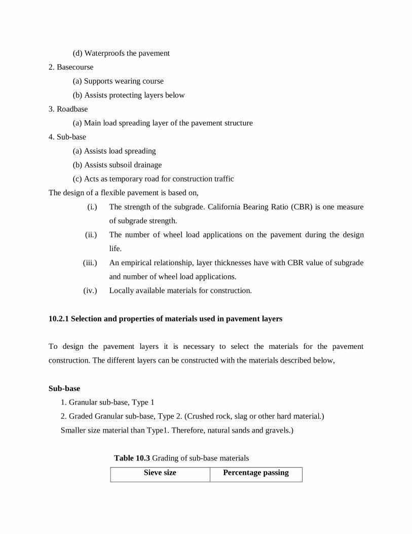
Table 10.3 Grading of sub-base materials

Sieve size Percentage passing

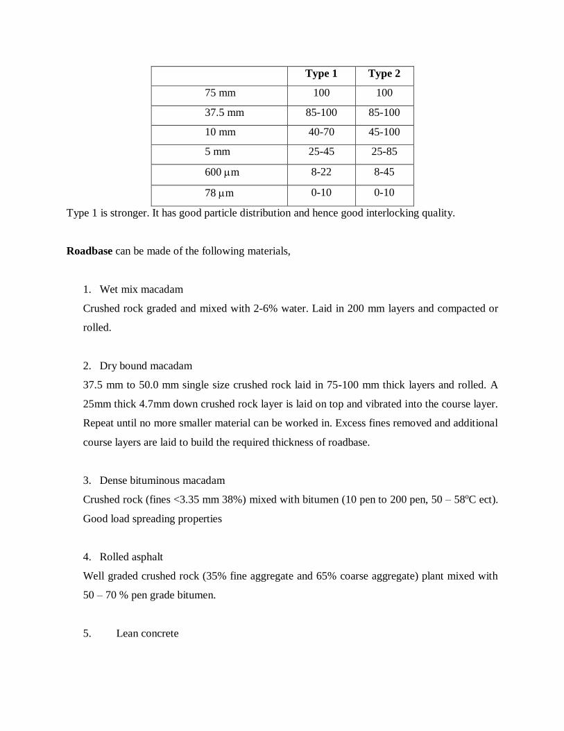
Type 1 Type 2

75 mm 100 100

37.5 mm 85-100 85-100

10 mm 40-70 45-100

5 mm 25-45 25-85

600 m 8-22 8-45

78m 0-10 0-10

Type 1 is stronger. It has good particle distribution and hence good interlocking quality.

Roadbase can be made of the following materials,

1. Wet mix macadam

Crushed rock graded and mixed with 2-6% water. Laid in 200 mm layers and compacted or

rolled.

2. Dry bound macadam

37.5 mm to 50.0 mm single size crushed rock laid in 75-100 mm thick layers and rolled. A

25mm thick 4.7mm down crushed rock layer is laid on top and vibrated into the course layer.

Repeat until no more smaller material can be worked in. Excess fines removed and additional

course layers are laid to build the required thickness of roadbase.

3. Dense bituminous macadam

Crushed rock (fines <3.35 mm 38%) mixed with bitumen (10 pen to 200 pen, 50 – 58oC ect).

Good load spreading properties

4. Rolled asphalt

Well graded crushed rock (35% fine aggregate and 65% coarse aggregate) plant mixed with

50 – 70 % pen grade bitumen.

5. Lean concrete

6. Cement bound roadbase

7. Soil cement and cement bound granular road base. Mixtures of soil or granular material

and cement, laid full depth in one layer and rolled.

Surfacing has either the wearing course only or wearing course with a base course.

1. Wearing course

(a) Bituminous surface dressing and a layer of chippings <10 mm. Rolled and excess

chippings removed.

(b) Double bituminous surface treatment. Tack coat, aggregate layer, rolled. Bitumen layer,

aggregate later rolled followed by bituminous surface dressing.

(c) Hot rolled asphalt. The Strongest and durable. Made of high fines. Laid 40 mm thick with

20 mm coated chippings rolled into the surface for better skid resistance.

2. Basecourse

(a) Open textured macadam. Coarse graded, no fines <3.35 mm. Thickness 60 – 80 mm for

40mm. Thickness 35 – 50 mm for 20mm.

(b) Dense basecourse

Well graded crushed rock (35% fine aggregate and 65% coarse aggregate), Thickness 60 – 80

mm for 40mm. Thickness 50 – 60 mm for 28 mm. Thickness 35 – 50 mm for 20 mm.

(c) Rolled asphalt basecourse.

Thickness 50 – 75 mm layer of rolled asphalt

10.2.2 C B R Test

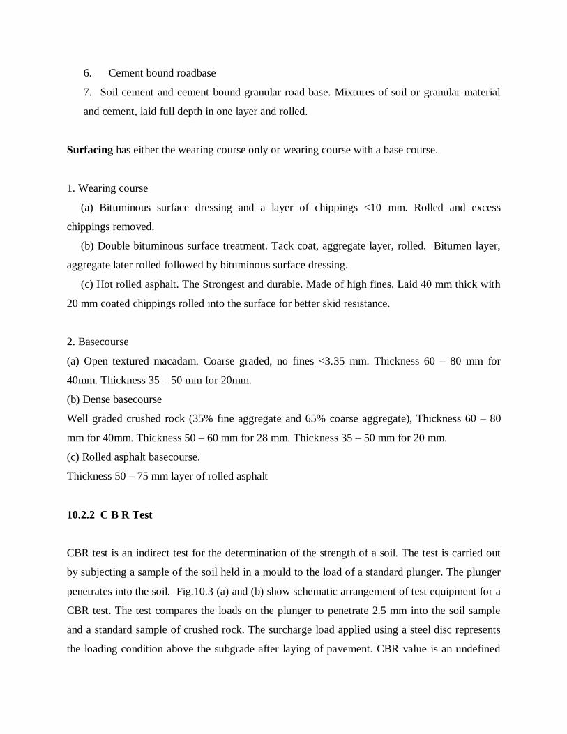
CBR test is an indirect test for the determination of the strength of a soil. The test is carried out

by subjecting a sample of the soil held in a mould to the load of a standard plunger. The plunger

penetrates into the soil. Fig.10.3 (a) and (b) show schematic arrangement of test equipment for a

CBR test. The test compares the loads on the plunger to penetrate 2.5 mm into the soil sample

and a standard sample of crushed rock. The surcharge load applied using a steel disc represents

the loading condition above the subgrade after laying of pavement. CBR value is an undefined

index of strength which depends on the soil condition at the time of testing. It is given by the

ratio expressed as percentage of load for 2.5mm of penetration in soil sample to load for same

penetration in standard crushed rock sample.

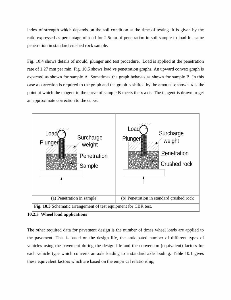
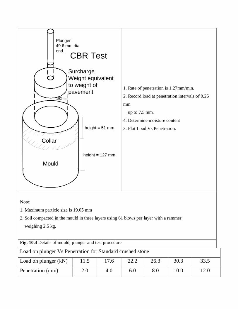
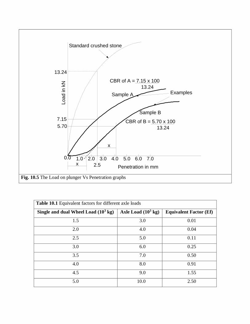
Fig. 10.4 shows details of mould, plunger and test procedure. Load is applied at the penetration

rate of 1.27 mm per min. Fig. 10.5 shows load vs penetration graphs. An upward convex graph is

expected as shown for sample A. Sometimes the graph behaves as shown for sample B. In this

case a correction is required to the graph and the graph is shifted by the amount x shown. x is the

point at which the tangent to the curve of sample B meets the x axis. The tangent is drawn to get

an approximate correction to the curve.

Load

Penetration

PlungerSurcharge

weight

Sample

Load

Penetration

PlungerSurcharge

weight

Crushed rock

(a) Penetration in sample (b) Penetration in standard crushed rock

Fig. 10.3 Schematic arrangement of test equipment for CBR test.

10.2.3 Wheel load applications

The other required data for pavement design is the number of times wheel loads are applied to

the pavement. This is based on the design life, the anticipated number of different types of

vehicles using the pavement during the design life and the conversion (equivalent) factors for

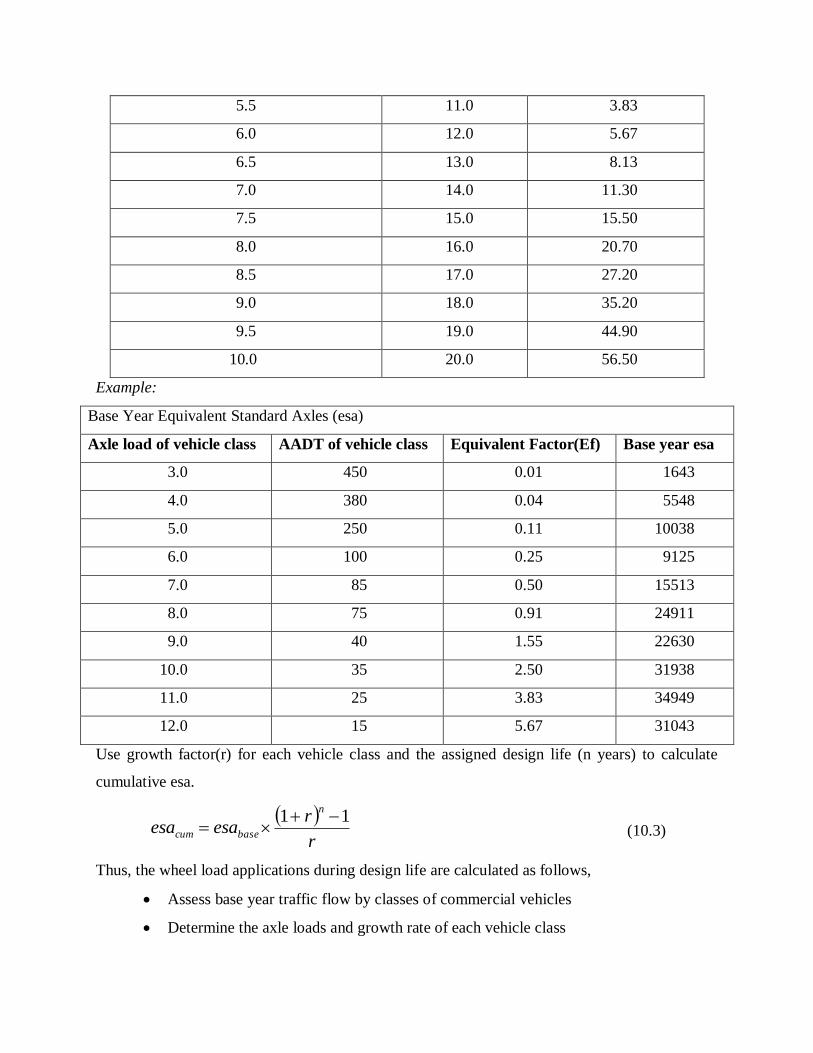
each vehicle type which converts an axle loading to a standard axle loading. Table 10.1 gives

these equivalent factors which are based on the empirical relationship,

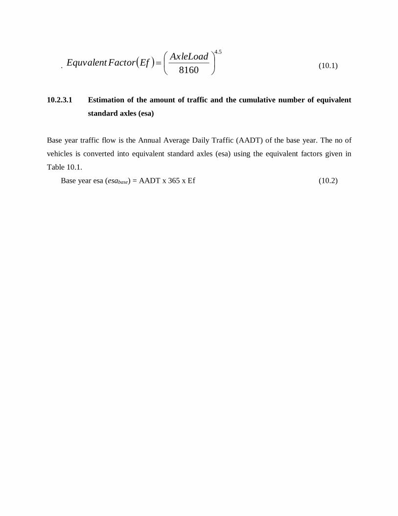
. 5.4

8160

AxleLoadEfFactorEquvalent (10.1)

10.2.3.1 Estimation of the amount of traffic and the cumulative number of equivalent

standard axles (esa)

Base year traffic flow is the Annual Average Daily Traffic (AADT) of the base year. The no of

vehicles is converted into equivalent standard axles (esa) using the equivalent factors given in

Table 10.1.

Base year esa (esabase) = AADT x 365 x Ef (10.2)

Surcharge

Weight equivalent

to weight of

pavement

Plunger

49.6 mm dia

end.

height = 51 mm

height = 127 mm

152 mm

Mould

Collar

CBR Test

1. Rate of penetration is 1.27mm/min.

2. Record load at penetration intervals of 0.25

mm

up to 7.5 mm.

4. Determine moisture content

3. Plot Load Vs Penetration.

Note:

1. Maximum particle size is 19.05 mm

2. Soil compacted in the mould in three layers using 61 blows per layer with a rammer

weighing 2.5 kg.

Fig. 10.4 Details of mould, plunger and test procedure

Load on plunger Vs Penetration for Standard crushed stone

Load on plunger (kN) 11.5 17.6 22.2 26.3 30.3 33.5

Penetration (mm) 2.0 4.0 6.0 8.0 10.0 12.0

2.5

1.0 2.0 3.0 4.0 5.0 6.0 7.0x

x

Sample A

Sample B

0.0

Penetration in mm

Loa

d in k

N

13.24

7.15

5.70

Examples

Standard crushed stone

CBR of A = 7.15 x 100

13.24

CBR of B = 5.70 x 100

13.24

Fig. 10.5 The Load on plunger Vs Penetration graphs

Table 10.1 Equivalent factors for different axle loads

Single and dual Wheel Load (103 kg) Axle Load (103 kg) Equivalent Factor (Ef)

1.5 3.0 0.01

2.0 4.0 0.04

2.5 5.0 0.11

3.0 6.0 0.25

3.5 7.0 0.50

4.0 8.0 0.91

4.5 9.0 1.55

5.0 10.0 2.50

5.5 11.0 3.83

6.0 12.0 5.67

6.5 13.0 8.13

7.0 14.0 11.30

7.5 15.0 15.50

8.0 16.0 20.70

8.5 17.0 27.20

9.0 18.0 35.20

9.5 19.0 44.90

10.0 20.0 56.50

Example:

Base Year Equivalent Standard Axles (esa)

Axle load of vehicle class AADT of vehicle class Equivalent Factor(Ef) Base year esa

3.0 450 0.01 1643

4.0 380 0.04 5548

5.0 250 0.11 10038

6.0 100 0.25 9125

7.0 85 0.50 15513

8.0 75 0.91 24911

9.0 40 1.55 22630

10.0 35 2.50 31938

11.0 25 3.83 34949

12.0 15 5.67 31043

Use growth factor(r) for each vehicle class and the assigned design life (n years) to calculate

cumulative esa.

r

resaesa

n

basecum

11 (10.3)

Thus, the wheel load applications during design life are calculated as follows,

Assess base year traffic flow by classes of commercial vehicles

Determine the axle loads and growth rate of each vehicle class

Apply the equivalent axle load factors and growth rates to base year traffic flow to

determine the pavement damaging effect [equivalent standard axles, (esa)] during the

design life.

The esacum can be directly used to find the thicknesses of pavement layers if the design charts of

Road Note 29 are employed. In order to use the design charts of Road Note 31

Table 10.2 Traffic and subgrade strength classes.

Traffic Classes Subgrade Strength Classes

Traffic Class 106 esa Range Subgrade Strength Class Range of CBR %

T1 <0.3 S1 2

T2 0.3 – 0.7 S2 3-4

T3 0.7 – 1.5 S3 5-7

T4 1.5 – 3.0 S4 8-14

T5 3.0 – 6.0 S5 15-29

T6 6.0 – 10.0 S6 30

T7 10.0 – 17.0

T8 17.0 – 30.0

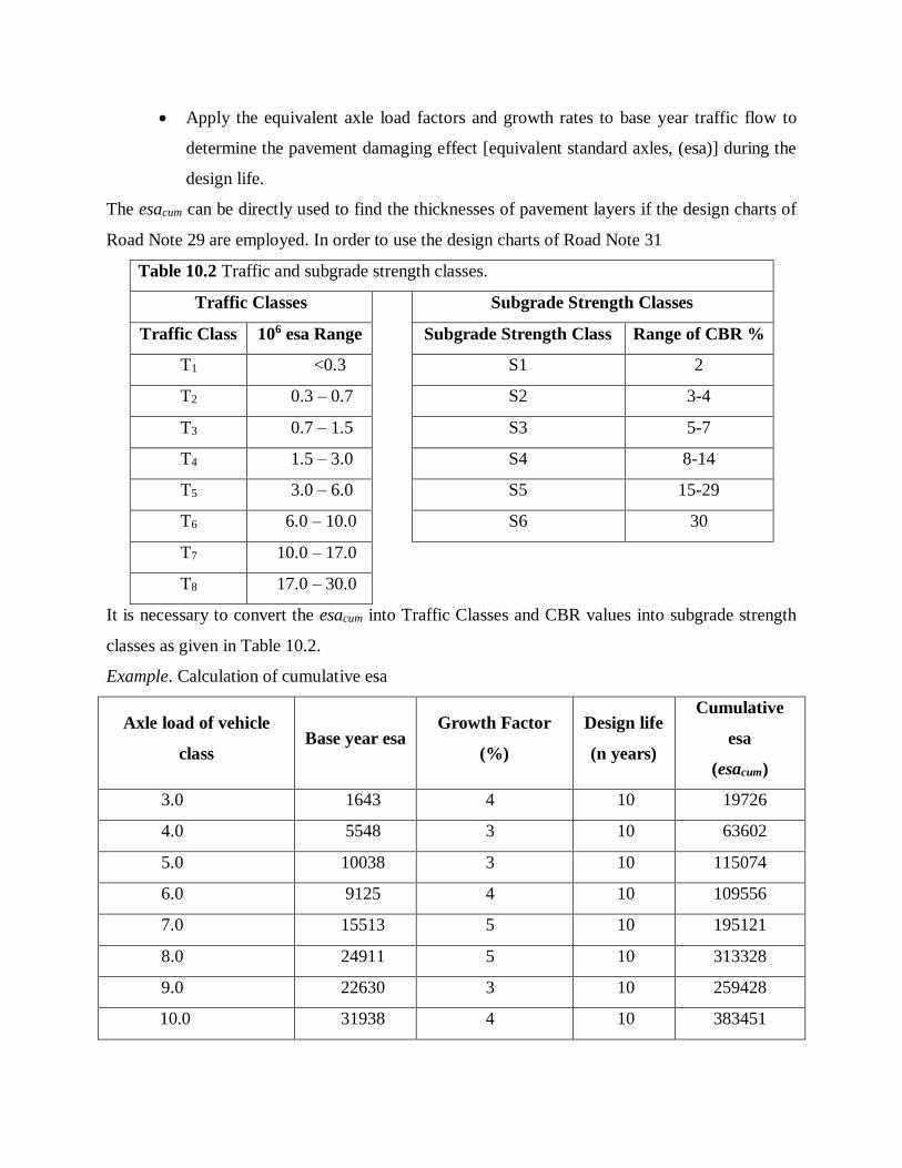
It is necessary to convert the esacum into Traffic Classes and CBR values into subgrade strength

classes as given in Table 10.2.

Example. Calculation of cumulative esa

Axle load of vehicle

class Base year esa

Growth Factor

(%)

Design life

(n years)

Cumulative

esa

(esacum)

3.0 1643 4 10 19726

4.0 5548 3 10 63602

5.0 10038 3 10 115074

6.0 9125 4 10 109556

7.0 15513 5 10 195121

8.0 24911 5 10 313328

9.0 22630 3 10 259428

10.0 31938 4 10 383451

11.0 34949 4 10 419601

12.0 31043 5 10 390456

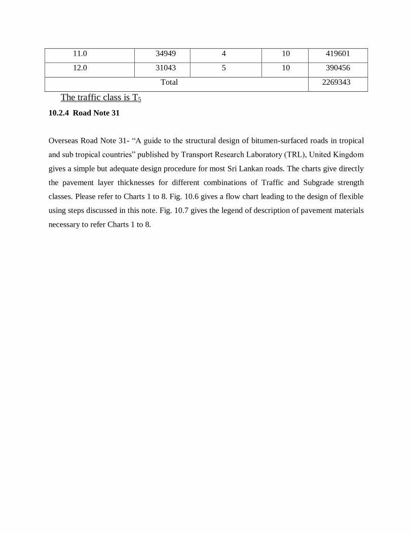
Total 2269343

The traffic class is T5

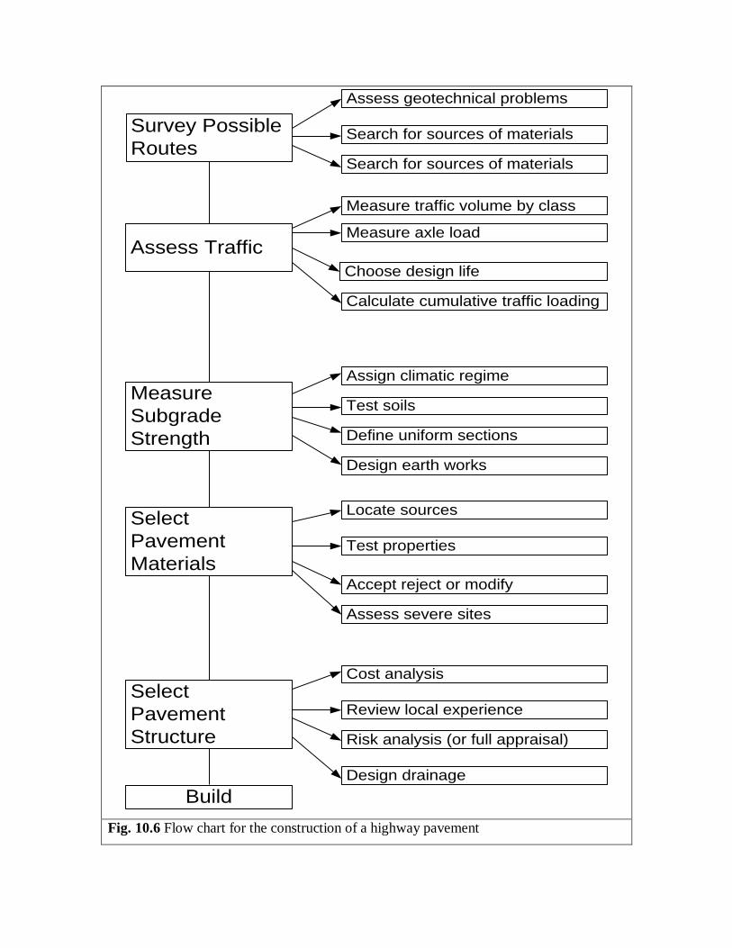
10.2.4 Road Note 31

Overseas Road Note 31- “A guide to the structural design of bitumen-surfaced roads in tropical

and sub tropical countries” published by Transport Research Laboratory (TRL), United Kingdom

gives a simple but adequate design procedure for most Sri Lankan roads. The charts give directly

the pavement layer thicknesses for different combinations of Traffic and Subgrade strength

classes. Please refer to Charts 1 to 8. Fig. 10.6 gives a flow chart leading to the design of flexible

using steps discussed in this note. Fig. 10.7 gives the legend of description of pavement materials

necessary to refer Charts 1 to 8.

Survey Possible

Routes

Assess Traffic

Measure

Subgrade

Strength

Select

Pavement

Materials

Select

Pavement

Structure

Build

Assess geotechnical problems

Search for sources of materials

Search for sources of materials

Measure traffic volume by class

Measure axle load

Choose design life

Calculate cumulative traffic loading

Locate sources

Assign climatic regime

Test soils

Define uniform sections

Design earth works

Test properties

Accept reject or modify

Assess severe sites

Cost analysis

Review local experience

Risk analysis (or full appraisal)

Design drainage

Fig. 10.6 Flow chart for the construction of a highway pavement