Introduction to graph mining and its application The First NIDA Business Analytics and Data Sciences Contest/Conference วันที่ 1-2 กันยายน 2559 ณ อาคารนวมินทราธิราช สถาบันบัณฑิตพัฒนบริหารศาสตร์ https://businessanalyticsnida.wordpress.com https://www.facebook.com/BusinessAnalyticsNIDA/ ผู้ช่วยศาสตราจารย์ ดร.วรพล พงษ์เพ็ชร มหาวิทยาลัยธุรกิจบัณฑิตย์ Graph เป็น Visualization ที่เราใช้กันอย่างแพร่หลาย โดยเฉพาะ ใน Social Network Analysis การทาเหมืองกราฟคืออะไร มีเทคนิคและวิธีการอย่างไรบ้าง มีงานวิจัยอะไรที่น่าสนใจ มีใครนามาประยุกต์ใช้ในธุรกิจอย่างไร ถ้าจะเริ่มทาเหมืองกราฟควรจะเตรียมอย่างไร นวมินทราธิราช 3001 วันที่ 2 กันยายน 2559 13.30-14.30 น.

Welcome message from author
This document is posted to help you gain knowledge. Please leave a comment to let me know what you think about it! Share it to your friends and learn new things together.
Transcript
Introduction to graph mining and its application
The First NIDA Business Analytics and Data Sciences Contest/Conferenceวันที่ 1-2 กันยายน 2559 ณ อาคารนวมินทราธิราช สถาบันบัณฑิตพัฒนบริหารศาสตร์
https://businessanalyticsnida.wordpress.comhttps://www.facebook.com/BusinessAnalyticsNIDA/
ผู้ช่วยศาสตราจารย์ ดร.วรพล พงษ์เพ็ชร มหาวิทยาลยัธุรกิจบัณฑิตย์
Graph เป็น Visualization ที่เราใช้กันอย่างแพร่หลาย โดยเฉพาะใน Social Network Analysis
การท าเหมืองกราฟคืออะไร มเีทคนิคและวิธีการอย่างไรบ้าง มีงานวิจัยอะไรที่น่าสนใจ มีใครน ามาประยุกต์ใช้ในธุรกิจอย่างไร ถ้าจะเริ่มท าเหมืองกราฟควรจะเตรียมอย่างไร
นวมินทราธิราช 3001 วันที่ 2 กันยายน 2559 13.30-14.30 น.
Graph Mining - Motivation, Applications and Algorithms
Adopted from
Graph mining seminar of Prof. Ehud Gudes
Fall 2008/9
Outline
• Introduction• Motivation and applications of Graph Mining• Mining Frequent Subgraphs – Transaction setting
– BFS/Apriori Approach (FSG and others)– DFS Approach (gSpan and others)– Greedy Approach
• Mining Frequent Subgraphs – Single graph setting– The support issue– The path-based algorithm

What is Data Mining?
Data Mining also known as Knowledge Discovery in Databases (KDD) is the process of extracting useful hidden information from very large databases in an unsupervised manner.
Mining Frequent Patterns:What is it good for?
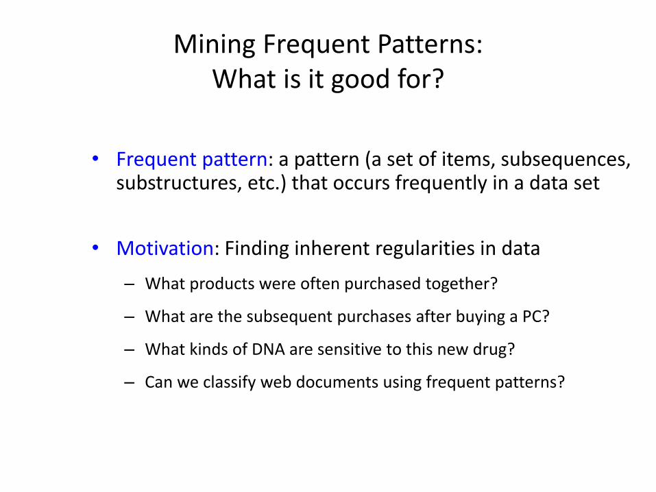
• Frequent pattern: a pattern (a set of items, subsequences, substructures, etc.) that occurs frequently in a data set
• Motivation: Finding inherent regularities in data
– What products were often purchased together?
– What are the subsequent purchases after buying a PC?
– What kinds of DNA are sensitive to this new drug?
– Can we classify web documents using frequent patterns?
The Apriori principle: Downward closure Property
• All subsets of a frequent itemset must also be frequent– Because any transaction that contains X must also contains subset of X.
• If we have already verified that X is infrequent,
there is no need to count X supersets because they must be infrequent too.

Outline
• Introduction• Motivation and applications of Graph Mining• Mining Frequent Subgraphs – Transaction setting
– BFS/Apriori Approach (FSG and others)– DFS Approach (gSpan and others)– Greedy Approach
• Mining Frequent Subgraphs – Single graph setting– The support issue– Path mining algorithm

What Graphs are good for?
• Most of existing data mining algorithms are based on transaction representation, i.e., sets of items.
• Datasets with structures, layers, hierarchy and/or geometry often do not fit well in this transaction setting. For e.g.
– Numerical simulations
– 3D protein structures
– Chemical Compounds
– Generic XML files.
Graph Based Data Mining
• Graph Mining is the problem of discovering repetitive subgraphs occurring in the input graphs.
• Motivation:
– finding subgraphs capable of compressing the data by abstracting instances of the substructures.
– identifying conceptually interesting patterns
Why Graph Mining?
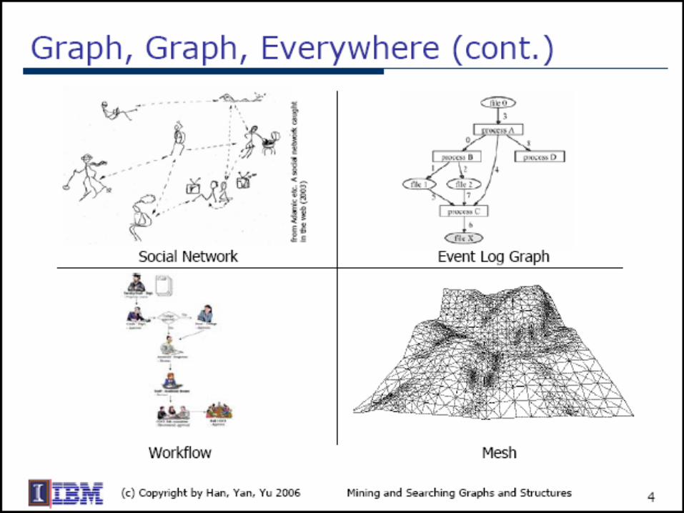
• Graphs are everywhere
– Chemical compounds (Cheminformatics)
– Protein structures, biological pathways/networks (Bioinformactics)
– Program control flow, traffic flow, and workflow analysis
– XML databases, Web, and social network analysis
• Graph is a general model
– Trees, lattices, sequences, and items are degenerated graphs
• Diversity of graphs
– Directed vs. undirected, labeled vs. unlabeled (edges & vertices), weighted, with
angles & geometry (topological vs. 2-D/3-D)
• Complexity of algorithms: many problems are of high complexity (NP
complete or even P-SPACE !)
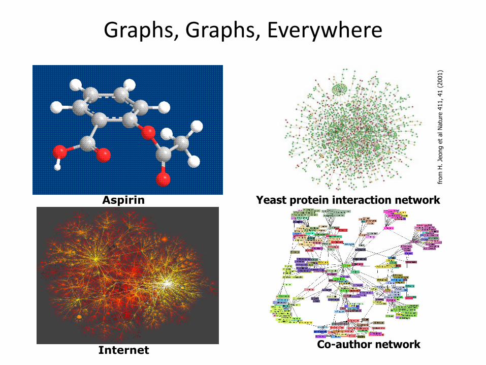
Graphs, Graphs, Everywhere
Aspirin Yeast protein interaction network
from
H.
Jeong e
t al N
atu
re 4
11, 41 (
2001)
InternetCo-author network
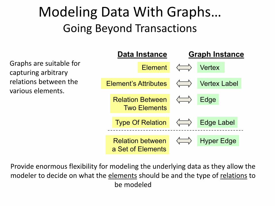
Modeling Data With Graphs…Going Beyond Transactions
Graphs are suitable for capturing arbitrary relations between the various elements.
VertexElement
Element’s Attributes
Relation Between
Two Elements
Type Of Relation
Vertex Label
Edge Label
Edge
Data Instance Graph Instance
Relation between
a Set of Elements
Hyper Edge
Provide enormous flexibility for modeling the underlying data as they allow the modeler to decide on what the elements should be and the type of relations to
be modeled
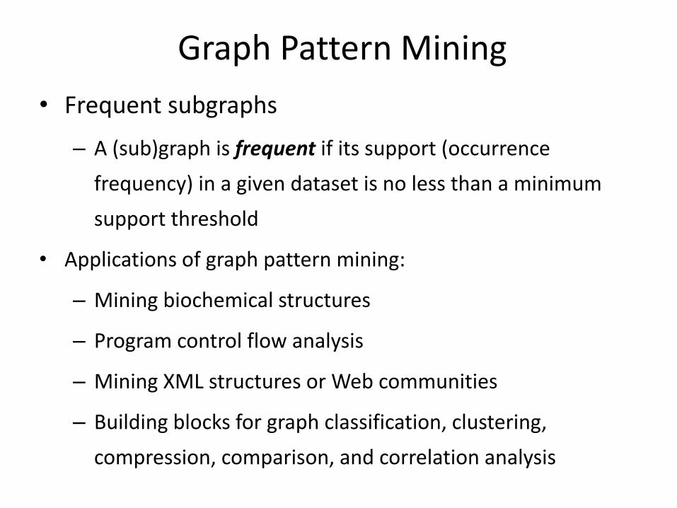
Graph Pattern Mining
• Frequent subgraphs
– A (sub)graph is frequent if its support (occurrence
frequency) in a given dataset is no less than a minimum
support threshold
• Applications of graph pattern mining:
– Mining biochemical structures
– Program control flow analysis
– Mining XML structures or Web communities
– Building blocks for graph classification, clustering,
compression, comparison, and correlation analysis

Example 1
GRAPH DATASET
FREQUENT PATTERNS(MIN SUPPORT IS 2)
(T1) (T2) (T3)
(1) (2)

Example 2GRAPH DATASET
FREQUENT PATTERNS(MIN SUPPORT IS 2)
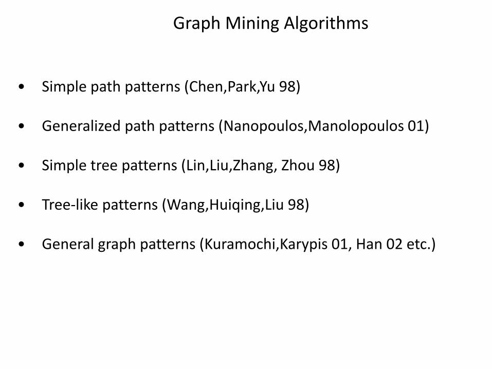
Graph Mining Algorithms
• Simple path patterns (Chen,Park,Yu 98)
• Generalized path patterns (Nanopoulos,Manolopoulos 01)
• Simple tree patterns (Lin,Liu,Zhang, Zhou 98)
• Tree-like patterns (Wang,Huiqing,Liu 98)
• General graph patterns (Kuramochi,Karypis 01, Han 02 etc.)

Graph mining methods
• Apriori-based approach
• Pattern-growth approach

Apriori-Based Approach
…
G
G1
G2
Gn
k-graph(k+1)-graph
G’
G’’
join
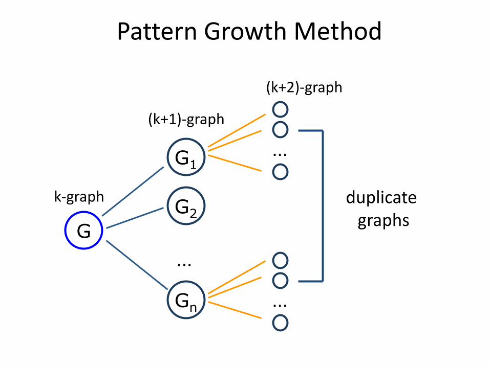
Pattern Growth Method
…
G
G1
G2
Gn
k-graph
(k+1)-graph
…
(k+2)-graph
…
duplicate graphs
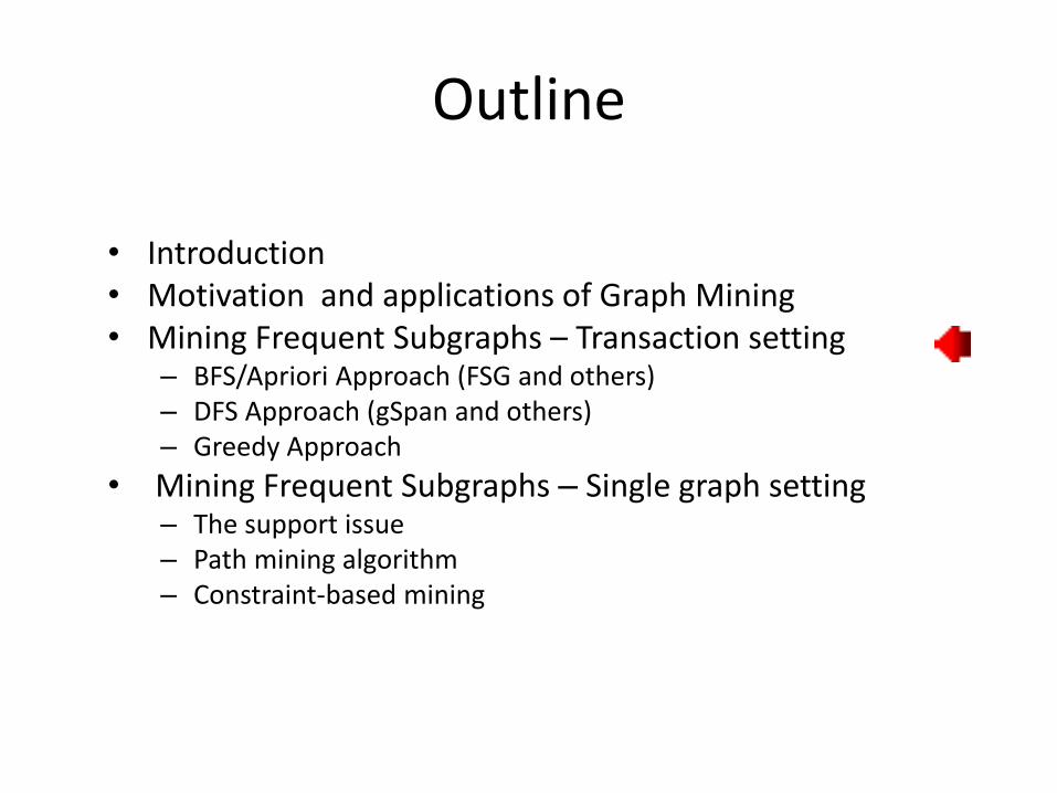
Outline
• Introduction• Motivation and applications of Graph Mining• Mining Frequent Subgraphs – Transaction setting
– BFS/Apriori Approach (FSG and others)– DFS Approach (gSpan and others)– Greedy Approach
• Mining Frequent Subgraphs – Single graph setting– The support issue– Path mining algorithm– Constraint-based mining
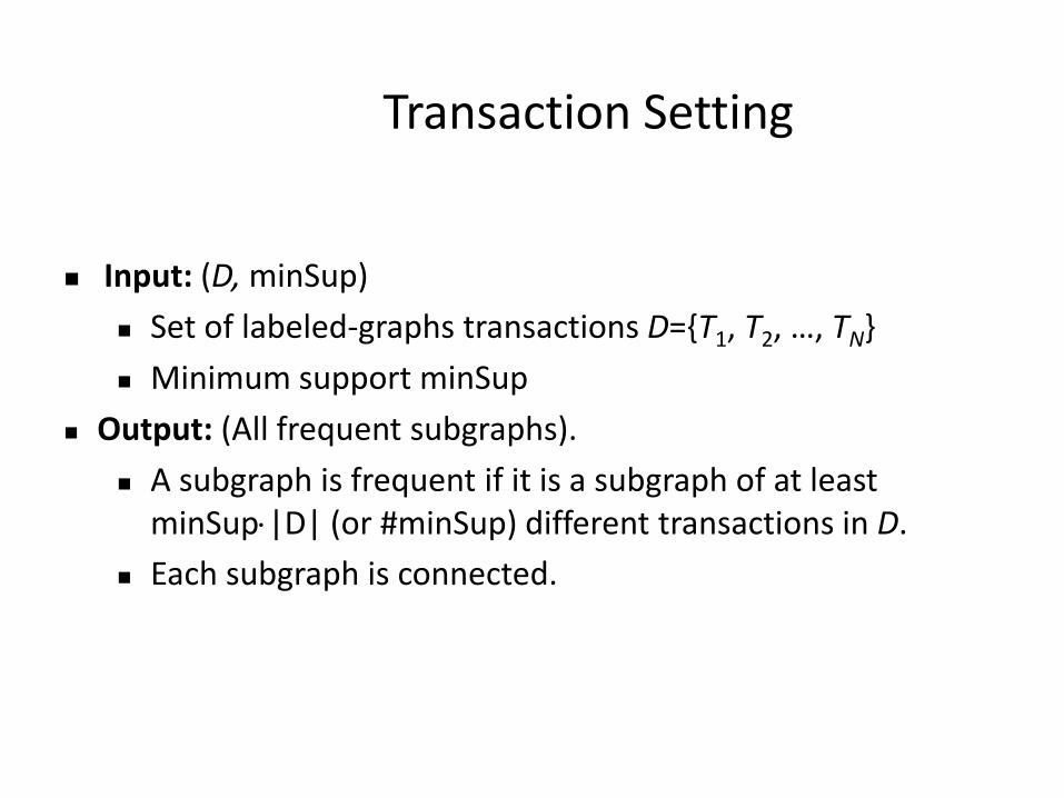
Transaction Setting
Input: (D, minSup)
Set of labeled-graphs transactions D={T1, T2, …, TN}
Minimum support minSup
Output: (All frequent subgraphs).
A subgraph is frequent if it is a subgraph of at least minSup|D| (or #minSup) different transactions in D.
Each subgraph is connected.
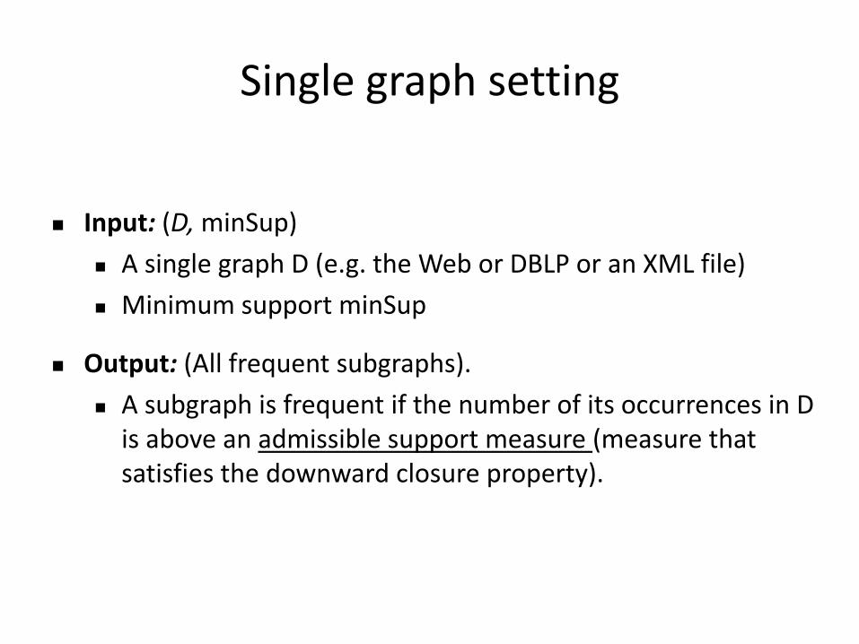
Single graph setting
Input: (D, minSup)
A single graph D (e.g. the Web or DBLP or an XML file)
Minimum support minSup
Output: (All frequent subgraphs).
A subgraph is frequent if the number of its occurrences in D is above an admissible support measure (measure that satisfies the downward closure property).
Graph Mining: Transaction Setting
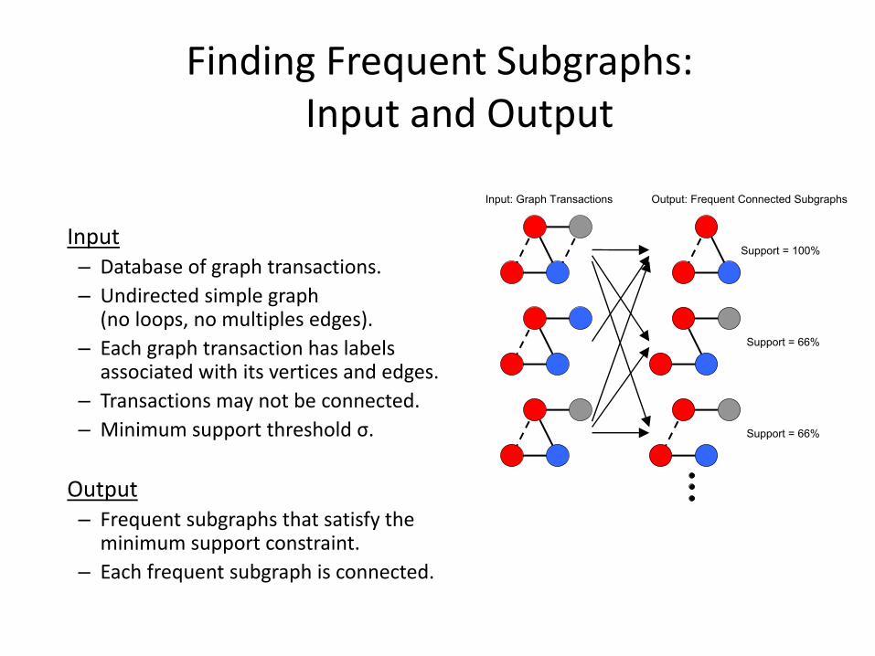
Finding Frequent Subgraphs:Input and Output
Input– Database of graph transactions.
– Undirected simple graph (no loops, no multiples edges).
– Each graph transaction has labels associated with its vertices and edges.
– Transactions may not be connected.
– Minimum support threshold σ.
Output– Frequent subgraphs that satisfy the
minimum support constraint.
– Each frequent subgraph is connected.
Support = 100%
Support = 66%
Support = 66%
Input: Graph Transactions Output: Frequent Connected Subgraphs

Different Approaches for GM
• Apriori Approach– FSG– Path Based
• DFS Approach– gSpan
• Greedy Approach – Subdue
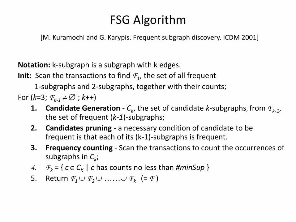
FSG Algorithm[M. Kuramochi and G. Karypis. Frequent subgraph discovery. ICDM 2001]
Notation: k-subgraph is a subgraph with k edges.
Init: Scan the transactions to find F1, the set of all frequent
1-subgraphs and 2-subgraphs, together with their counts;
For (k=3; Fk-1 ; k++)
1. Candidate Generation - Ck, the set of candidate k-subgraphs, from Fk-1, the set of frequent (k-1)-subgraphs;
2. Candidates pruning - a necessary condition of candidate to be frequent is that each of its (k-1)-subgraphs is frequent.
3. Frequency counting - Scan the transactions to count the occurrences of subgraphs in Ck;
4. Fk = { c CK | c has counts no less than #minSup }
5. Return F1 F2 …… Fk (= F )
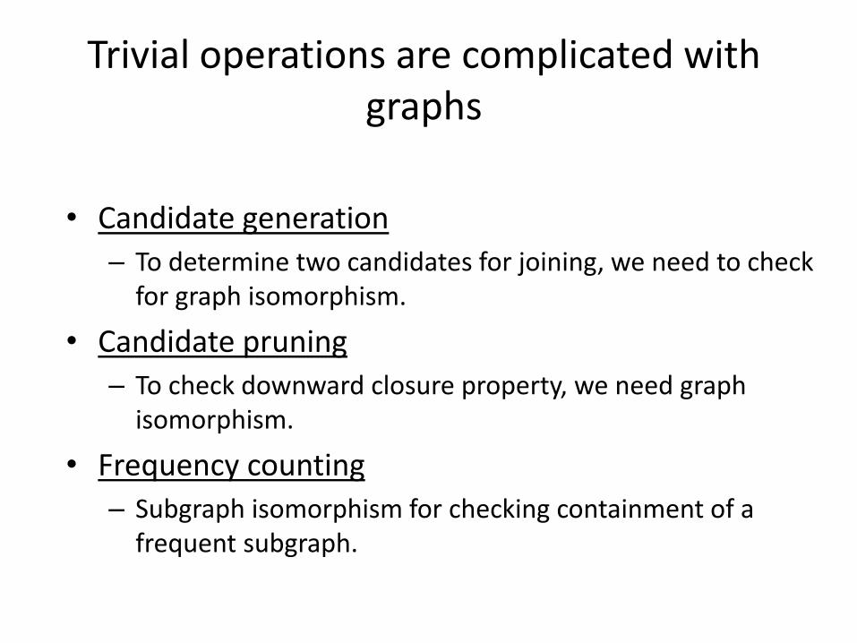
Trivial operations are complicated with graphs
• Candidate generation
– To determine two candidates for joining, we need to check for graph isomorphism.
• Candidate pruning
– To check downward closure property, we need graph isomorphism.
• Frequency counting
– Subgraph isomorphism for checking containment of a frequent subgraph.
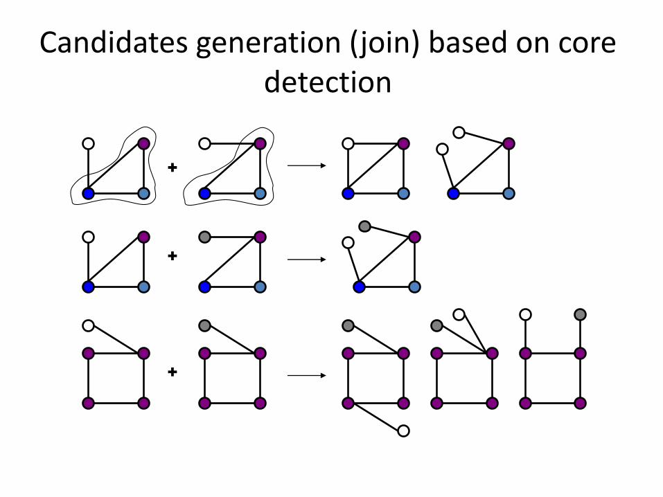
Candidates generation (join) based on core detection
+
+
+
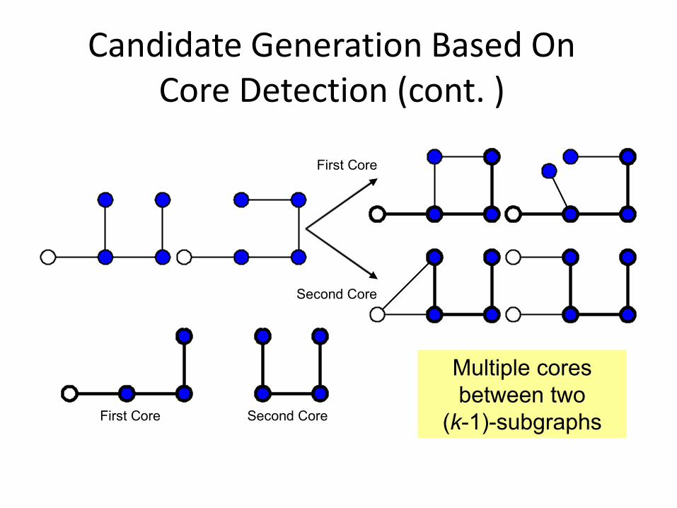
Candidate Generation Based On Core Detection (cont. )
First Core
Second Core
First Core Second Core
Multiple cores
between two
(k-1)-subgraphs
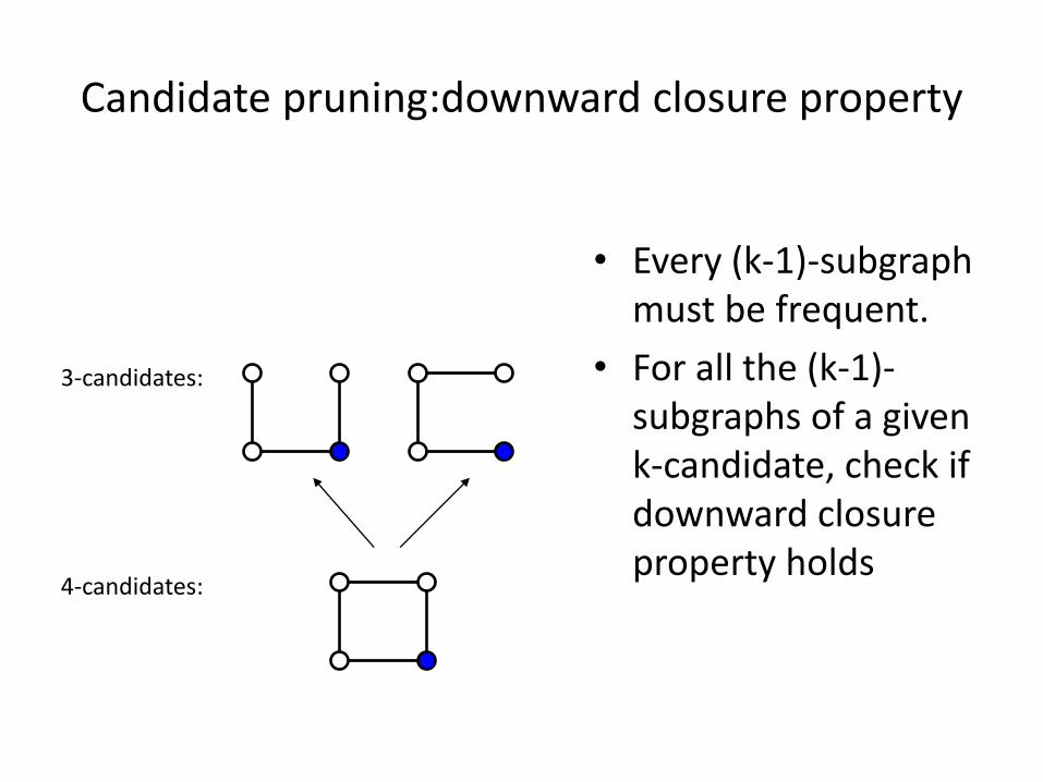
Candidate pruning:downward closure property
• Every (k-1)-subgraph must be frequent.
• For all the (k-1)-subgraphs of a given k-candidate, check if downward closure property holds
3-candidates:
4-candidates:

frequent1-subgraphs
3-candidates
4-candidates
. . . . . .
frequent2-subgraphs
frequent3-subgraphs
frequent4-subgraphs
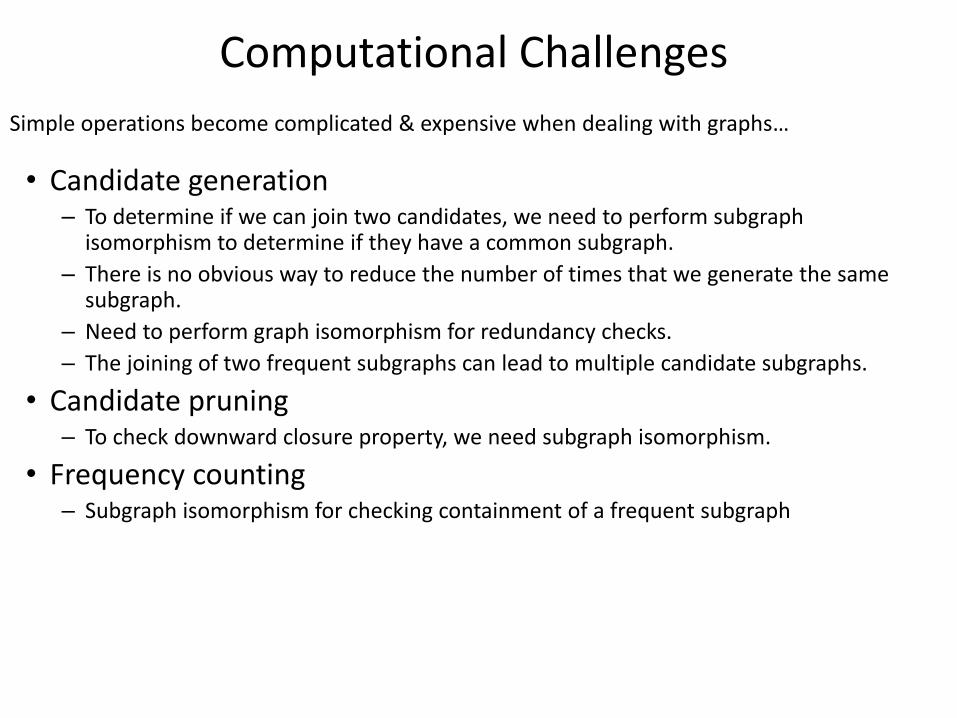
Computational Challenges
• Candidate generation– To determine if we can join two candidates, we need to perform subgraph
isomorphism to determine if they have a common subgraph.
– There is no obvious way to reduce the number of times that we generate the same subgraph.
– Need to perform graph isomorphism for redundancy checks.
– The joining of two frequent subgraphs can lead to multiple candidate subgraphs.
• Candidate pruning– To check downward closure property, we need subgraph isomorphism.
• Frequency counting– Subgraph isomorphism for checking containment of a frequent subgraph
Simple operations become complicated & expensive when dealing with graphs…

Computational Challenges
• Key to FSG’s computational efficiency:–Uses an efficient algorithm to determine a canonical labeling
of a graph and use these “strings” to perform identity checks (simple comparison of strings!).
–Uses a sophisticated candidate generation algorithm that reduces the number of times each candidate is generated.
–Uses an augmented TID-list based approach to speedup frequency counting.
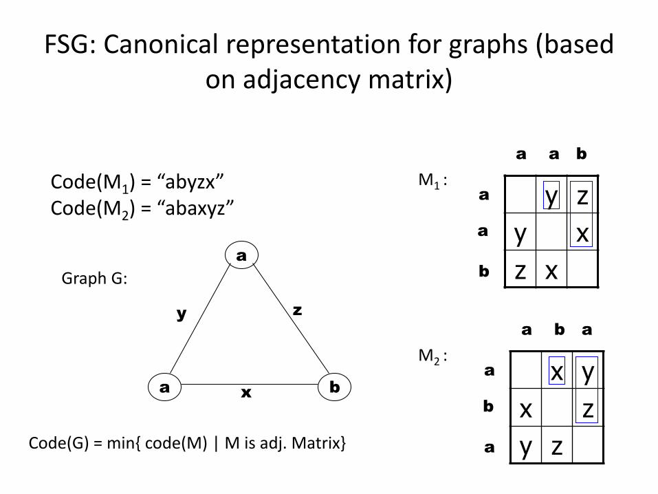
FSG: Canonical representation for graphs (based on adjacency matrix)
zy
xy
xz
a a b
a
a
b
Code(M1) = “abyzx”Code(M2) = “abaxyz”
yx
zx
zy
a b a
a
b
a
a
a
b
y z
x
Graph G:
Code(G) = min{ code(M) | M is adj. Matrix}
M1 :
M2 :
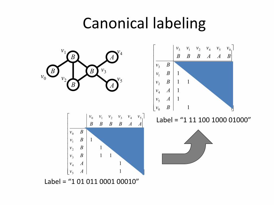
Canonical labeling
1
1
1111
11
111
1
5
4
3
2
1
0
543210
Av
Av
Bv
Bv
Bv
Bv
AABBBB
vvvvvv
1
1
1
11
111
1111
0
5
4
2
1
3
054213
Bv
Av
Av
Bv
Bv
Bv
BAABBB
vvvvvv
v0
B
v1B
v2B
v3B
v4A
v5A
Label = “1 01 011 0001 00010”
Label = “1 11 100 1000 01000”
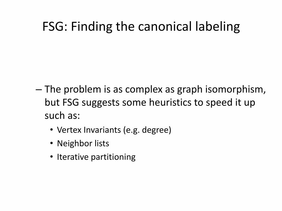
FSG: Finding the canonical labeling
– The problem is as complex as graph isomorphism, but FSG suggests some heuristics to speed it up such as:
• Vertex Invariants (e.g. degree)
• Neighbor lists
• Iterative partitioning
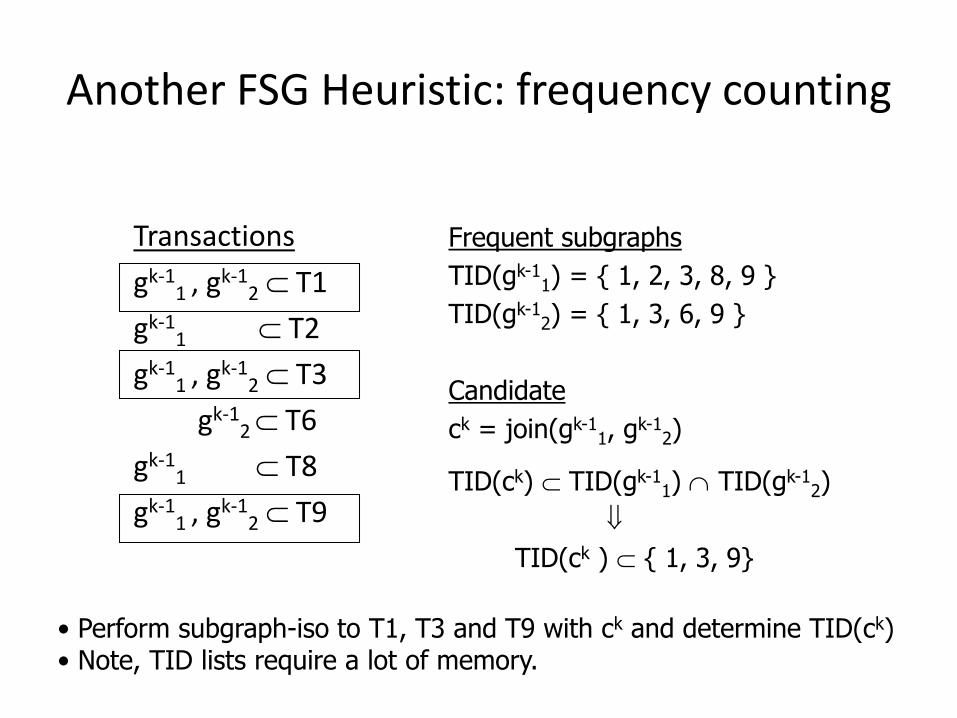
Another FSG Heuristic: frequency counting
Transactions
gk-11 , g
k-12 T1
gk-11 T2
gk-11 , g
k-12 T3
gk-12 T6
gk-11 T8
gk-11 , g
k-12 T9
Frequent subgraphs
TID(gk-11) = { 1, 2, 3, 8, 9 }
TID(gk-12) = { 1, 3, 6, 9 }
Candidate
ck = join(gk-11, g
k-12)
TID(ck) TID(gk-11) TID(gk-1
2)
TID(ck ) { 1, 3, 9}
• Perform subgraph-iso to T1, T3 and T9 with ck and determine TID(ck)• Note, TID lists require a lot of memory.
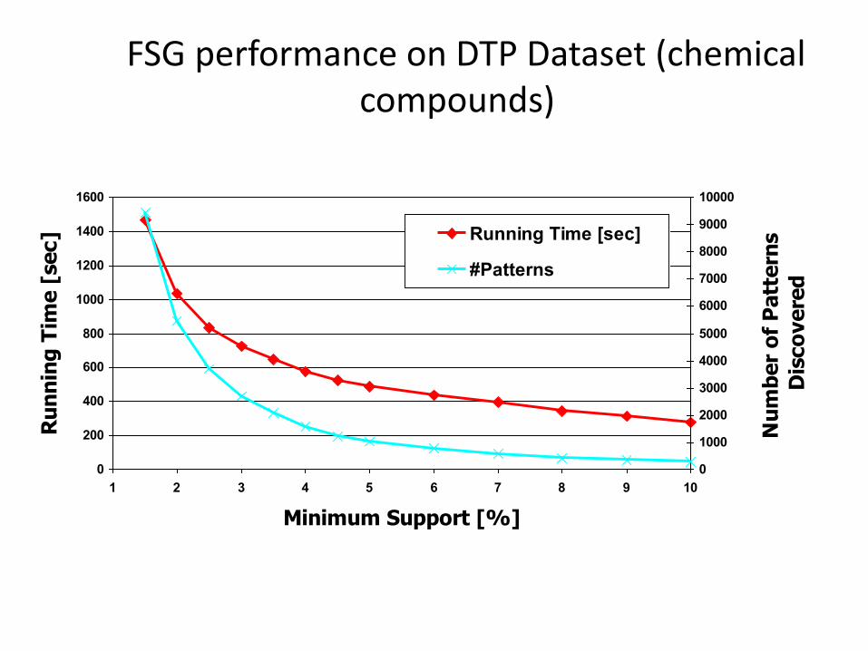
FSG performance on DTP Dataset (chemical compounds)
0
200
400
600
800
1000
1200
1400
1600
1 2 3 4 5 6 7 8 9 10
Minimum Support [%]
Ru
nn
ing
Tim
e [
sec]
0
1000
2000
3000
4000
5000
6000
7000
8000
9000
10000
Nu
mb
er
of
Patt
ern
s
Dis
co
vere
d
Running Time [sec]
#Patterns

Topology Is Not Enough (Sometimes)
• Graphs arising from physical domains have a strong geometric nature.– This geometry must be taken into
account by the data-mining algorithms.
• Geometric graphs.– Vertices have physical 2D and 3D
coordinates associated with them.
O
O
I
OH
H
H
H
H
H
H
H
H
H
H
H
H
H
H H
H
H
H
H
H
H
H
O
O
HH
H
H
H
HH
H
H
H
H
H
OH
HH
H
H
H H
H
H
H
H
H
H
H
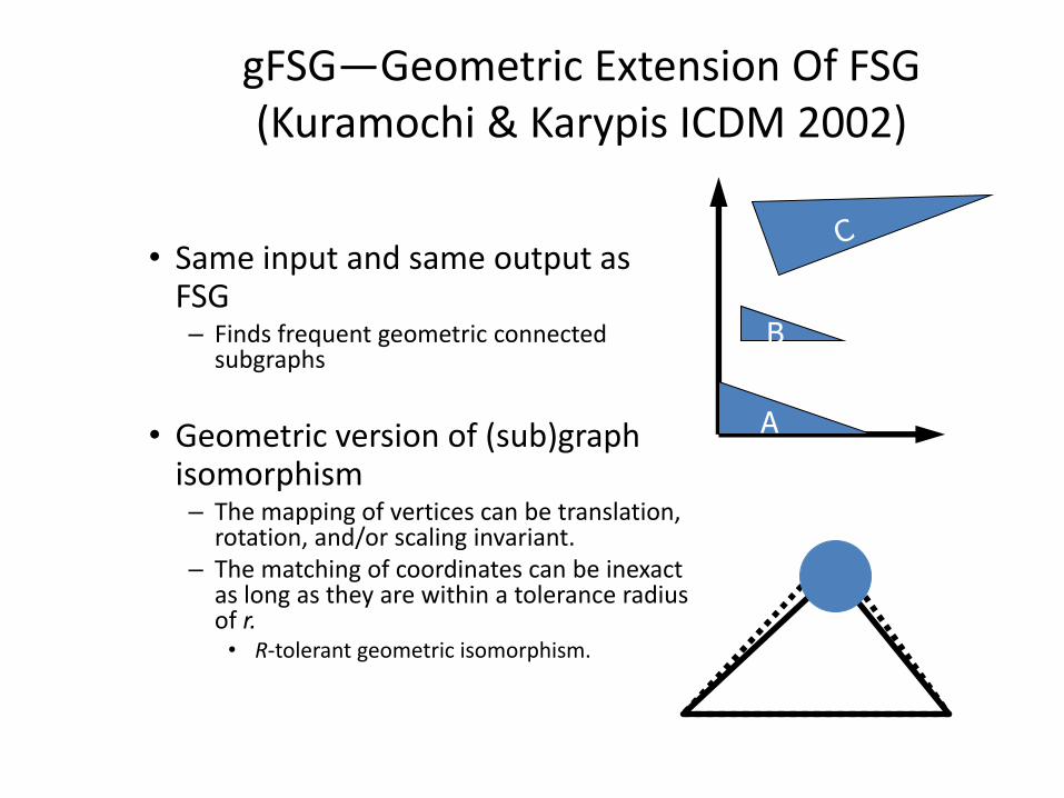
gFSG—Geometric Extension Of FSG (Kuramochi & Karypis ICDM 2002)
• Same input and same output as FSG– Finds frequent geometric connected
subgraphs
• Geometric version of (sub)graph isomorphism– The mapping of vertices can be translation,
rotation, and/or scaling invariant. – The matching of coordinates can be inexact
as long as they are within a tolerance radius of r. • R-tolerant geometric isomorphism.
A
B
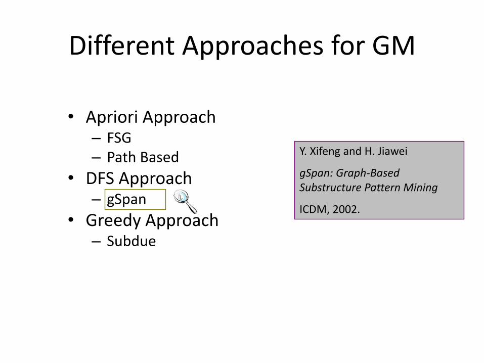
Different Approaches for GM
• Apriori Approach– FSG– Path Based
• DFS Approach– gSpan
• Greedy Approach – Subdue
Y. Xifeng and H. Jiawei
gSpan: Graph-Based Substructure Pattern Mining
ICDM, 2002.

part1:
Define the Tree Search Space (TSS)
Part2:
Find all frequent graphs
by exploring TSS
gSpan outline
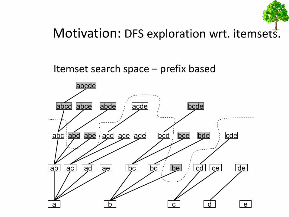
Motivation: DFS exploration wrt. itemsets.
Itemset search space – prefix based
ba c d e
ab ac ad ae bc bd be cd ce de
abc abd abe acd ace ade bcd bce bde cde
abcd abce abde acde bcde
abcde
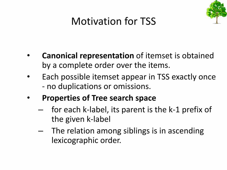
Motivation for TSS
• Canonical representation of itemset is obtained by a complete order over the items.
• Each possible itemset appear in TSS exactly once - no duplications or omissions.
• Properties of Tree search space
– for each k-label, its parent is the k-1 prefix of the given k-label
– The relation among siblings is in ascending lexicographic order.

DFS Code representation
• Map each graph (2-Dim) to a sequential DFS Code (1-Dim).
• Lexicographically order the codes.
• Construct TSS based on the lexicographic order.

DFS Code construction
• Given a graph G. for each Depth First Search over graph G, construct the corresponding DFS-Code.
X
Y
X
Z
Z
aa
b
cb
d
v0X
Y
X
Z
Z
aa
b
cb
d
v0
v1
X
Y
X
Z
Z
a
a
b
cb
d
v0
v1
v2
X
Y
X
Z
Z
aa
b
cb
d
v0
v1
v2
X
Y
X
Z
Z
aa
b
c
bd
v0
v1
v2
v3
X
Y
X
Z
Z
a
a
b
cb
d
v0
v1
v2
v3
X
Y
X
Z
Z
aa
b
cb
d
v0
v1
v2
v3
v4
(0,1,X,a,Y) (1,2,Y,b,X) (2,0,X,a,X) (2,3,X,c,Z) (3,1,Z,b,Y) (1,4,Y,d,Z)
(a) (b) (c) (d) (e) (f) (g)
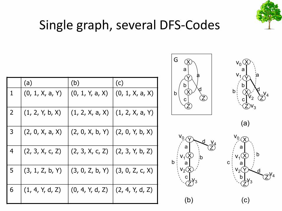
Single graph, several DFS-Codes
X
Y
X
Z
Z
aa
b
c
b d
v0
v1
v2
v3
v4
X
Y
X
Z
Z
aa
b
cb
d
Y
X
X
Z
Za
ba
c
dv0
v1
v2
v3
v4
b
X
X
Y
Z
Z
a
b
a
bd
v0
v1
v2
v3
v4
c
(a)
(b) (c)
(c)(b)(a)
(0, 1, X, a, X)(0, 1, Y, a, X)(0, 1, X, a, Y)1
(1, 2, X, a, Y)(1, 2, X, a, X)(1, 2, Y, b, X)2
(2, 0, Y, b, X)(2, 0, X, b, Y)(2, 0, X, a, X)3
(2, 3, Y, b, Z)(2, 3, X, c, Z)(2, 3, X, c, Z)4
(3, 0, Z, c, X)(3, 0, Z, b, Y)(3, 1, Z, b, Y)5
(2, 4, Y, d, Z)(0, 4, Y, d, Z)(1, 4, Y, d, Z)6
G
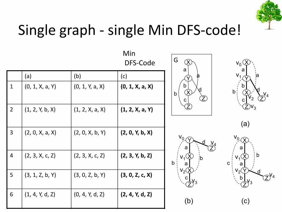
Single graph - single Min DFS-code!
X
Y
X
Z
Z
aa
b
c
b d
v0
v1
v2
v3
v4
X
Y
X
Z
Z
aa
b
cb
d
Y
X
X
Z
Za
ba
c
dv0
v1
v2
v3
v4
b
X
X
Y
Z
Z
a
b
a
bd
v0
v1
v2
v3
v4
c
(a)
(b) (c)
(c)(b)(a)
(0, 1, X, a, X)(0, 1, Y, a, X)(0, 1, X, a, Y)1
(1, 2, X, a, Y)(1, 2, X, a, X)(1, 2, Y, b, X)2
(2, 0, Y, b, X)(2, 0, X, b, Y)(2, 0, X, a, X)3
(2, 3, Y, b, Z)(2, 3, X, c, Z)(2, 3, X, c, Z)4
(3, 0, Z, c, X)(3, 0, Z, b, Y)(3, 1, Z, b, Y)5
(2, 4, Y, d, Z)(0, 4, Y, d, Z)(1, 4, Y, d, Z)6
MinDFS-Code G
Minimum DFS-Code
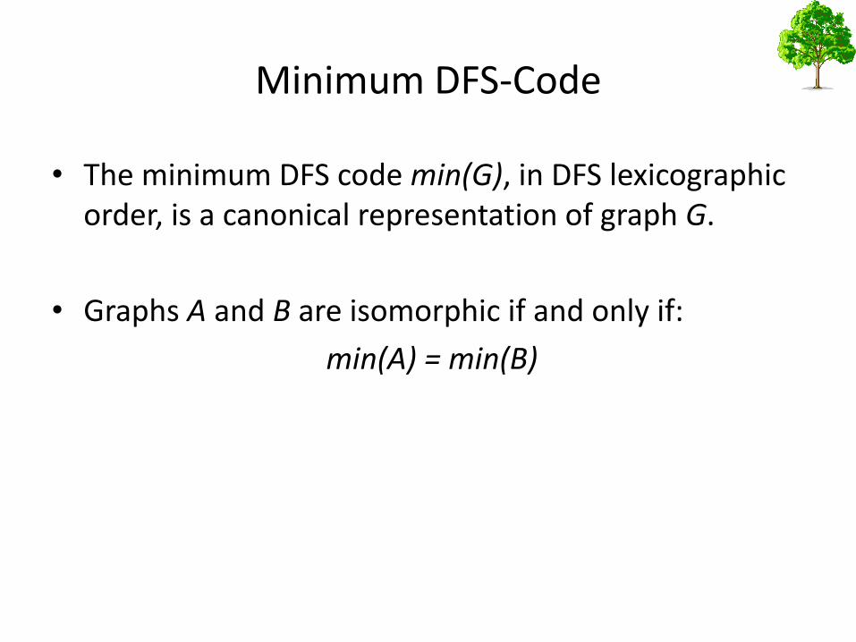
• The minimum DFS code min(G), in DFS lexicographic order, is a canonical representation of graph G.
• Graphs A and B are isomorphic if and only if:
min(A) = min(B)
DFS-Code Tree: parent-child relation
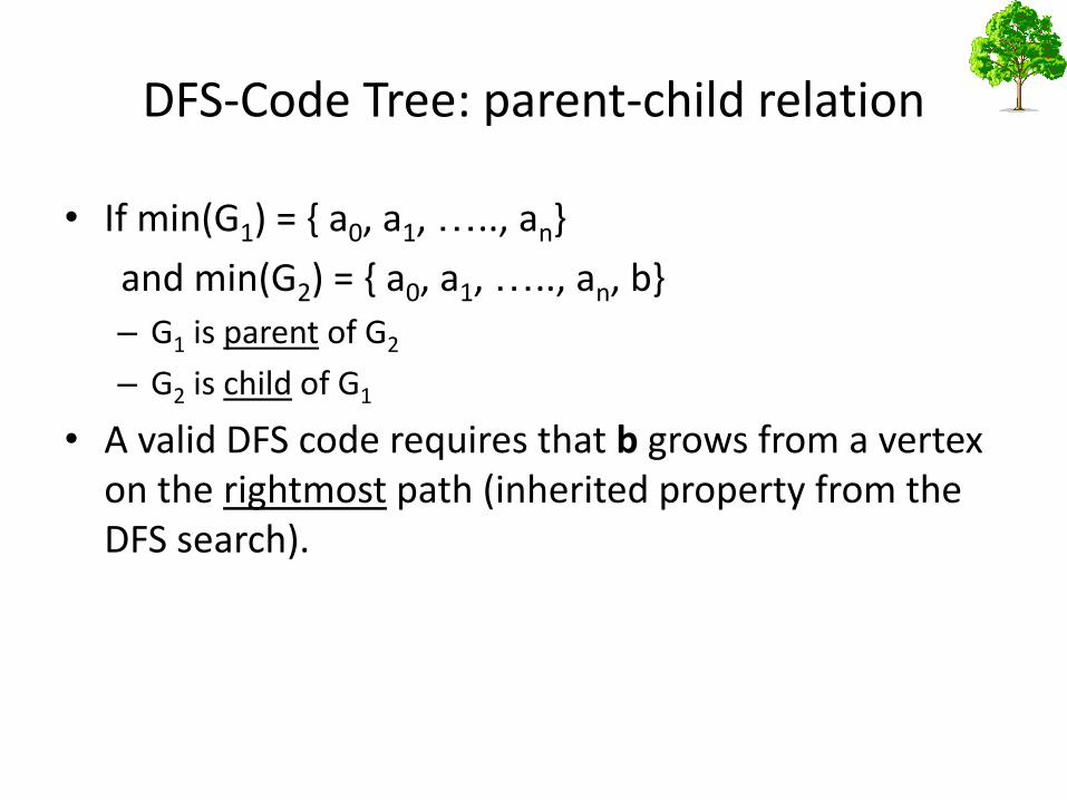
• If min(G1) = { a0, a1, ….., an}
and min(G2) = { a0, a1, ….., an, b}
– G1 is parent of G2
– G2 is child of G1
• A valid DFS code requires that b grows from a vertex on the rightmost path (inherited property from the DFS search).
X
Y
X
Z
Z
aa
b
cb
d
v0
v1
v2
v3
v4
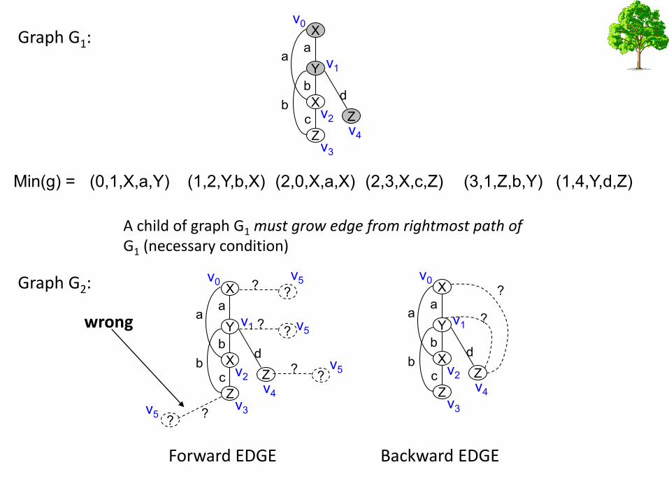
(0,1,X,a,Y) (1,2,Y,b,X) (2,0,X,a,X) (2,3,X,c,Z) (3,1,Z,b,Y) (1,4,Y,d,Z)
Graph G1:
Min(g) =
X
Y
X
Z
Z
aa
b
cb
d
v0
v1
v2
v3
v4
A child of graph G1 must grow edge from rightmost path of G1 (necessary condition)
?
?
?
?
?
?
v5
v5
v5
??v5
wrong
X
Y
X
Z
Z
aa
b
cb
d
v0
v1
v2
v3
v4
?
?
Forward EDGE Backward EDGE
Graph G2:
Search space: DFS code Tree
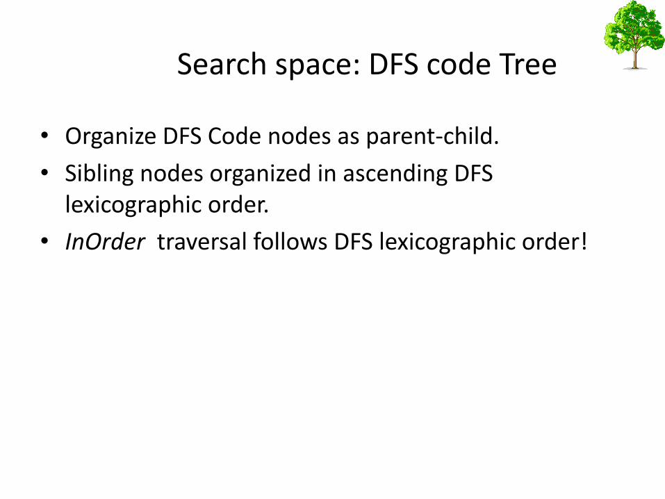
• Organize DFS Code nodes as parent-child.
• Sibling nodes organized in ascending DFS lexicographic order.
• InOrder traversal follows DFS lexicographic order!
C
C
A
C
C
C
B
C
C
B
B
B
B
B
C
B
C
A
A
A A
C
C
A
B
A
C
A
C
C
A
C
B
A
B
C
A A
C
A
B
C
0
1
2
3
0
1
2
3
0
1
2
3
0
1
23
0
1
23
0
1
2
3
0
1
2
0
1
2
0
1
0
1
0
1
0
1
0
1
2
0
1
2
0
1
2
0
1
2
0
1
2
0
1
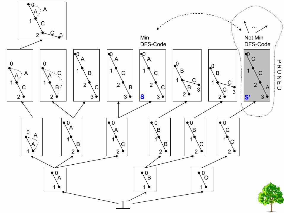
2 3 Not Min
DFS-Code
Min
DFS-Code
S
P R
U N
E D
…
A
S’
Tree pruning
• All of the descendants of infrequent node are infrequent also.
• All of the descendants of a not minimal DFS code are also not minimal DFS codes.
part1:
defining the Tree Search Space (TSS)
Part2:
gSpan Finds all frequent graphs
by Exploring TSS
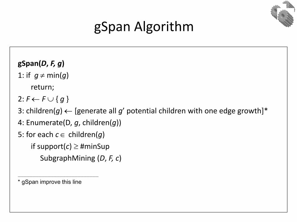
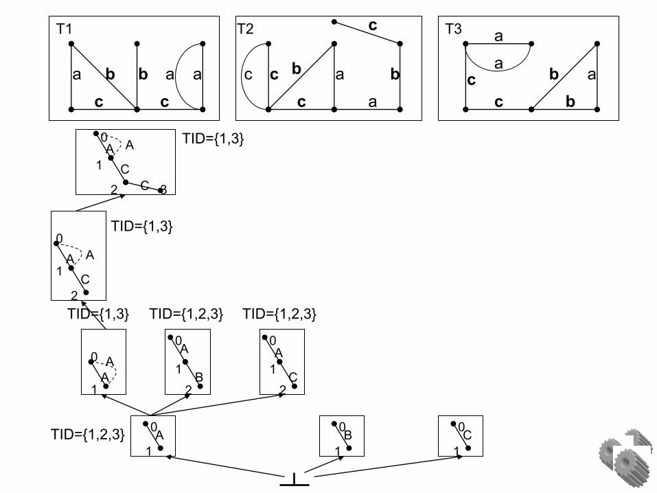
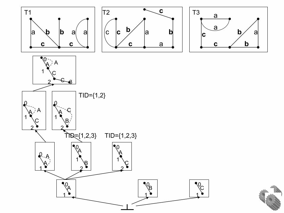
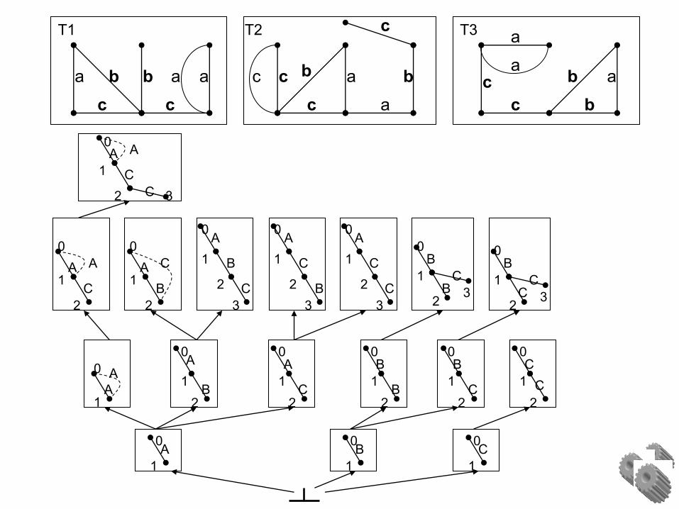
gSpan Algorithm
gSpan(D, F, g)
1: if g min(g)
return;
2: F F { g }
3: children(g) [generate all g’ potential children with one edge growth]*
4: Enumerate(D, g, children(g))
5: for each c children(g)
if support(c) #minSup
SubgraphMining (D, F, c)
___________________________
* gSpan improve this line
aaa
a
c aa
a
bb bb
b
b
c c c
c a
c
c
c
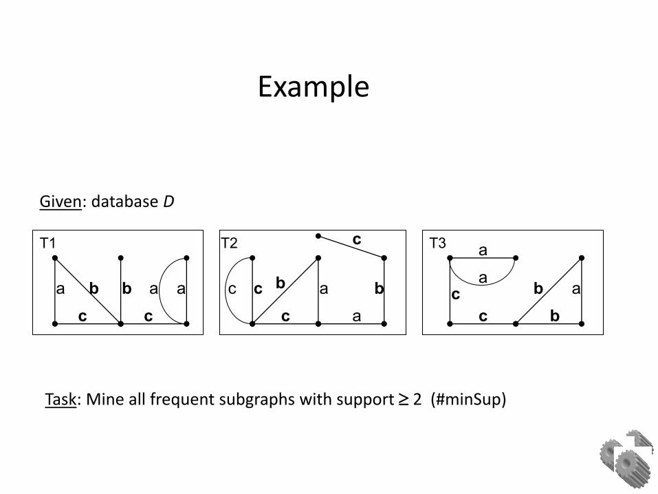
T2 T3T1
Given: database D
Task: Mine all frequent subgraphs with support 2 (#minSup)
Example
aaa
a
c aa
a
bb bb
b
b
c c c
c a
c
c
c
T2
A
A
A A
C
C
A
B
A
C
A A
C
0
1
2
0
1
0
1
0
1
2
0
1
2
0
1
2 3
A
T3T1
TID={1,3} TID={1,2,3} TID={1,2,3}
TID={1,3}
TID={1,2,3}
TID={1,3}
CB0
1
0
1
aaa
a
c aa
a
bb bb
b
b
c c c
c a
c
c
c
T2
CBA
A
A A
C
C
A
B
A
C
A A
C
A
B
C
0
1
2
0
1
2
0
1
0
1
0
1
0
1
0
1
2
0
1
2
0
1
2 3
A
T3T1
TID={1,2,3} TID={1,2,3}
TID={1,2}
aaa
a
c aa
a
bb bb
b
b
c c c
c a
c
c
c
T2
C
C
C
B
CC
B
B
B
B
BC
B
C
A
A
A A
C
C
A
B
A
C
A
C
C
A
C
B
A
B
C
A A
C
A
B
C
0
1
2
3
0
1
2
3
0
1
2
3
0
1
23
0
1
23
0
1
2
0
1
2
0
1
0
1
0
1
0
1
0
1
2
0
1
2
0
1
2
0
1
2
0
1
2
0
1
2 3
A
T3T1
gSpan Performance
• On synthetic datasets it was 6-10 times faster than FSG.
• On Chemical compounds datasets it was 15-100 times faster!
• But this was comparing to OLD versions of FSG!
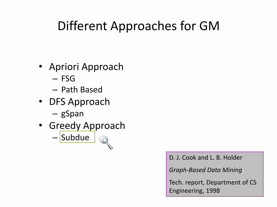
Different Approaches for GM
• Apriori Approach– FSG– Path Based
• DFS Approach– gSpan
• Greedy Approach – Subdue
D. J. Cook and L. B. Holder
Graph-Based Data Mining
Tech. report, Department of CS Engineering, 1998
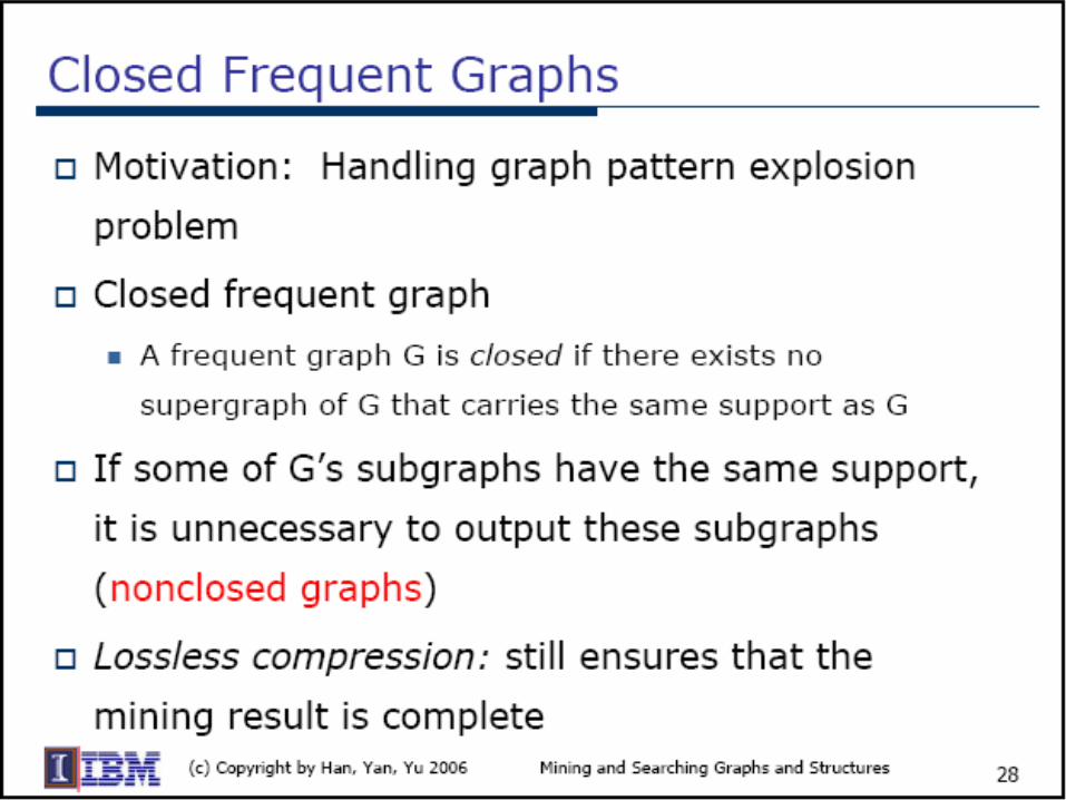
Graph Pattern Explosion Problem
• If a graph is frequent, all of its subgraphs are frequent ─ the
Apriori property
• An n-edge frequent graph may have 2n subgraphs.
• Among 422 chemical compounds which are confirmed to be
active in an AIDS antiviral screen dataset, there are 1,000,000
frequent graph patterns if the minimum support is 5%.

Subdue algorithm
• A greedy algorithm for finding some of the most prevalent subgraphs.
• This method is not complete, i.e. it may not obtain all frequent subgraphs, although it pays in fast execution.
Subdue algorithm (Cont.)
• It discovers substructures that compress the original
data and represent structural concepts in the data.
• Based on Beam Search - like BFS it progresses level by
level. Unlike BFS, however, beam search moves
downward only through the best W nodes at each
level. The other nodes are ignored.

Step 1: Create substructure for each unique vertex label
circle
rectangle
left
triangle
square
on
on
triangle
square
on
on
triangle
square
on
on
triangle
square
on
onleft
left left
left
Substructures:
triangle (4)
square (4)
circle (1)
rectangle (1)
Subdue algorithm: step 1
DB:
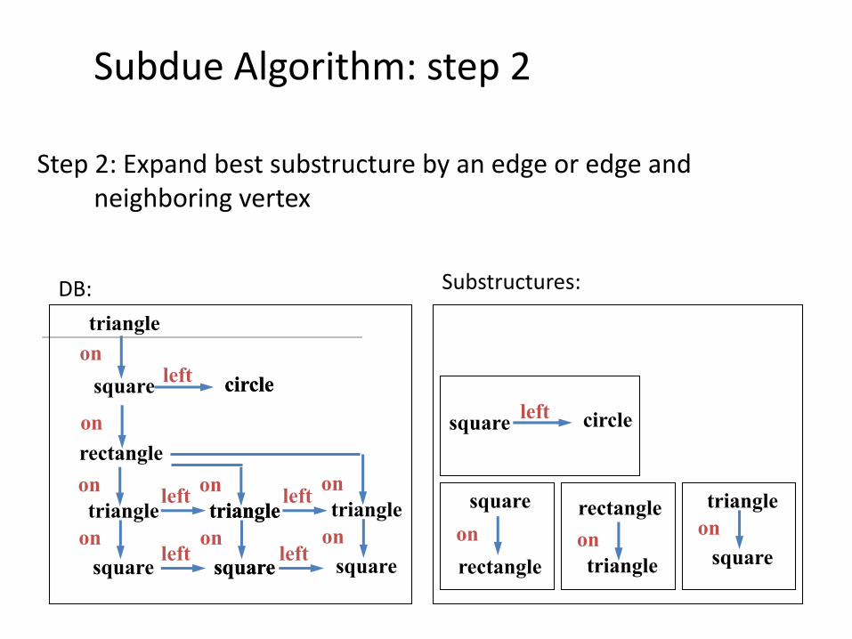
Subdue Algorithm: step 2
Step 2: Expand best substructure by an edge or edge and neighboring vertex
circle
rectangle
left
triangle
square
ontriangle
square
on
on
triangle
square
on
on
triangle
square
on
onleft
left left
left
triangle
square
on
on
circle
triangle
square
circleleftsquare
rectangle
square
on
rectangle
triangle
on
Substructures:DB:
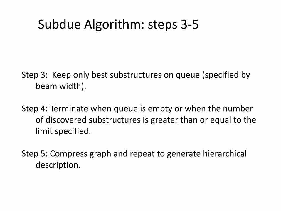
Step 3: Keep only best substructures on queue (specified by beam width).
Step 4: Terminate when queue is empty or when the number of discovered substructures is greater than or equal to the limit specified.
Step 5: Compress graph and repeat to generate hierarchical description.
Subdue Algorithm: steps 3-5
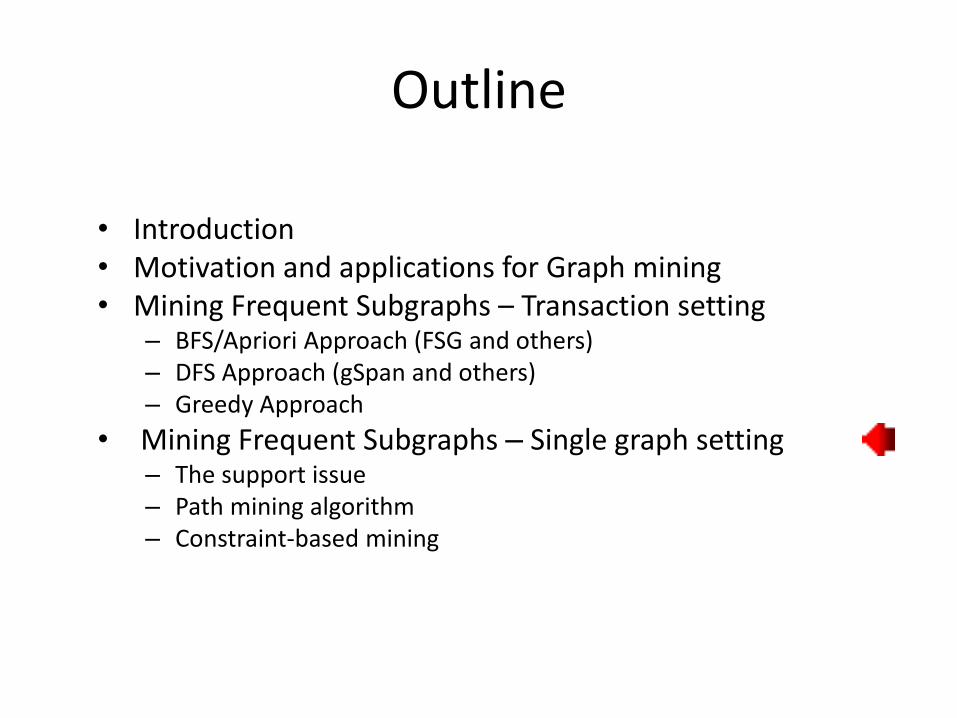
Outline
• Introduction• Motivation and applications for Graph mining• Mining Frequent Subgraphs – Transaction setting
– BFS/Apriori Approach (FSG and others)– DFS Approach (gSpan and others)– Greedy Approach
• Mining Frequent Subgraphs – Single graph setting– The support issue– Path mining algorithm– Constraint-based mining
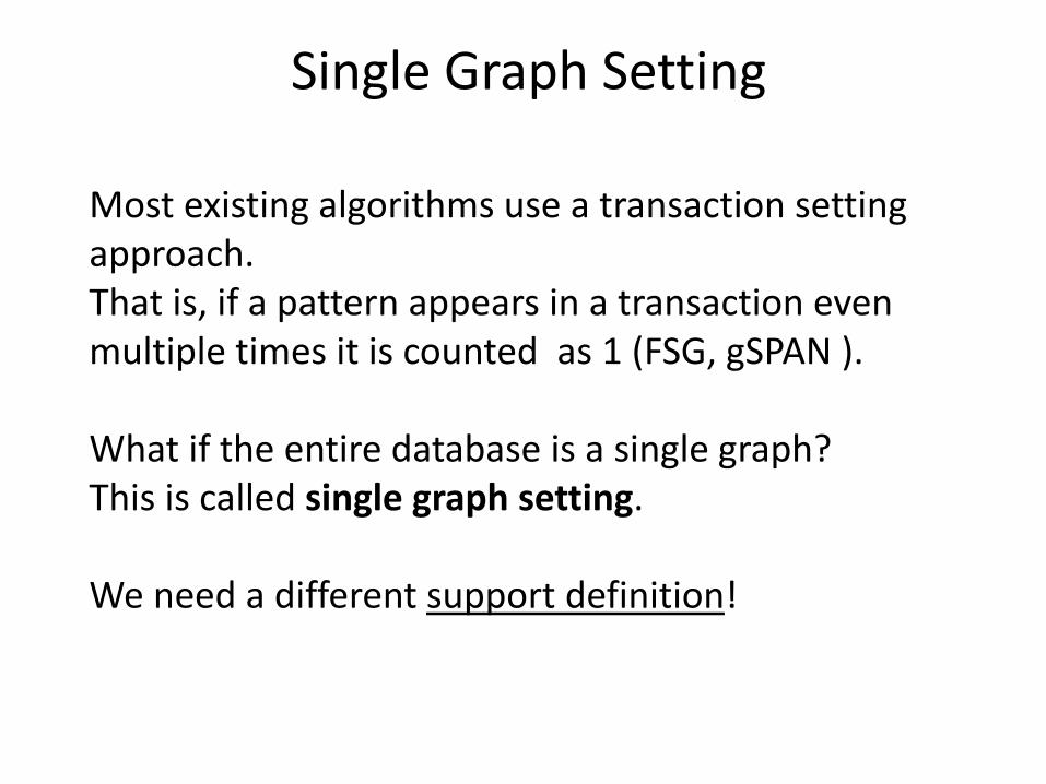
Single Graph Setting
Most existing algorithms use a transaction setting approach.That is, if a pattern appears in a transaction even multiple times it is counted as 1 (FSG, gSPAN ).
What if the entire database is a single graph?This is called single graph setting.
We need a different support definition!
Single graph setting - Motivation
Often the input is a single large graph.
Examples:
The web or portions of it.
A social network (e.g. a network of users communicating by email at BGU).
A large XML database such as DBLP or Movies database.
Mining large graph databases is very useful.

Support issue
Support measure is admissible if for any pattern P and any sub-pattern Q P support of P is not larger than support of Q.
Problem: the number of pattern appearances is not good!
Support issue
An instance graph of pattern P in database graph D is a graph whose nodes are pattern instances in D and they are connected by an edge when corresponding instances share an edge.

Support issue
Operations on instance graph:
• clique contraction: replace clique C by a single node c. Only the nodes adjacent to each node of C may be adjacent to c.
node expansion: replace node v by a new subgraph whose nodes may or may not be adjacent to the nodes adjacent to v.
node addition: add a new node to the graph and arbitrary edges between the new node and the old ones.
edge removal : remove an edge.
The main result
Theorem. A support measure S is an admissible support measure if and only if it is non-decreasing on instance graph of every pattern P under clique contraction, node expansion, node addition and edge removal.
Example of support measure - MIS
Maximum independent set size of instance graphMIS = _____________________________________
Number of edges in the database graph

Path mining algorithm (Vanetik, Gudes, Shimony)
Goal: find all frequent connected subgraphs of a database graph.
Basic approach: Apriori or BFS. The basic building block is a path not an edge. This works since any graph can be decomposed into
edge-disjoint paths.
Result: faster convergence of the algorithm.
Path-based mining algorithm
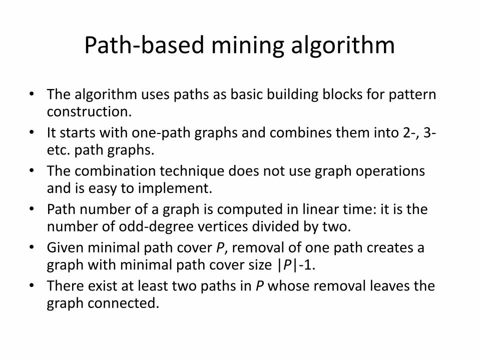
• The algorithm uses paths as basic building blocks for pattern construction.
• It starts with one-path graphs and combines them into 2-, 3-etc. path graphs.
• The combination technique does not use graph operations and is easy to implement.
• Path number of a graph is computed in linear time: it is the number of odd-degree vertices divided by two.
• Given minimal path cover P, removal of one path creates a graph with minimal path cover size |P|-1.
• There exist at least two paths in P whose removal leaves the graph connected.
More than one path cover for graph
1. Define a descriptor of each path based on node labels and node
degrees.
2. Use lexicographical order among descriptors to compare
between paths.
3. One graph can have several minimal path covers.
4. We only use path covers that are minimal w.r.t. lexicographical
order.
5. Removal of path from a lexicographically minimal path cover
leaves the cover lexicographically minimal.
Example: path descriptors
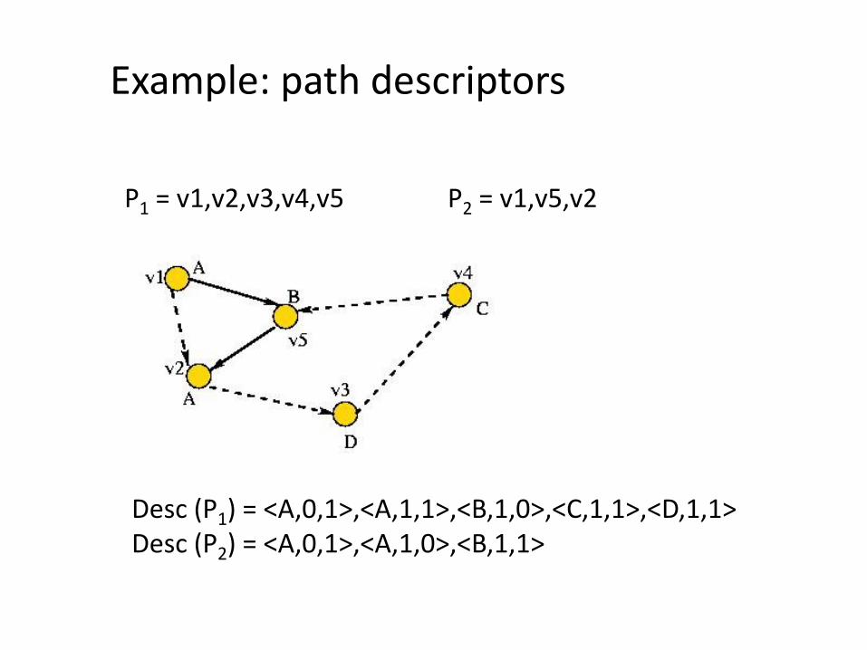
P1 = v1,v2,v3,v4,v5 P2 = v1,v5,v2
Desc (P1) = <A,0,1>,<A,1,1>,<B,1,0>,<C,1,1>,<D,1,1>Desc (P2) = <A,0,1>,<A,1,0>,<B,1,1>

Path mining algorithm
Phase 1: find all frequent 1-path graphs.
Phase 2: find all frequent 2-path graphs by“joining” frequent 1-path graphs.
Phase 3: find all frequent k-path graphs, k3,by “joining” pairs of frequent (k-1)-path graphs.
Main challenge: “join” must ensure soundness and completeness of the algorithm.
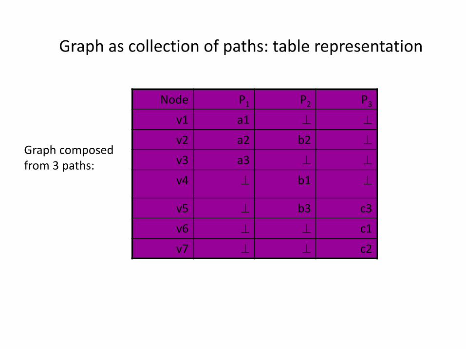
Graph as collection of paths: table representation
Node P1 P2 P3
v1 a1
v2 a2 b2
v3 a3
v4 b1
v5 b3 c3
v6 c1
v7 c2
Graph composedfrom 3 paths:
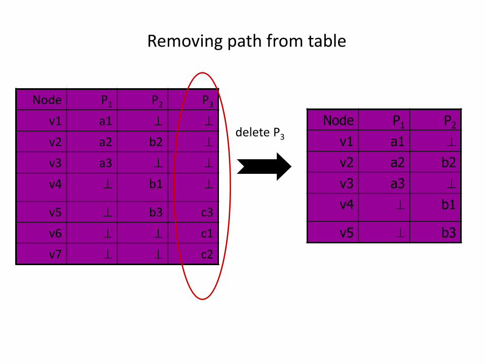
Removing path from table
Node P1 P2
v1 a1
v2 a2 b2
v3 a3
v4 b1
v5 b3
delete P3
Node P1 P2 P3
v1 a1
v2 a2 b2
v3 a3
v4 b1
v5 b3 c3
v6 c1
v7 c2
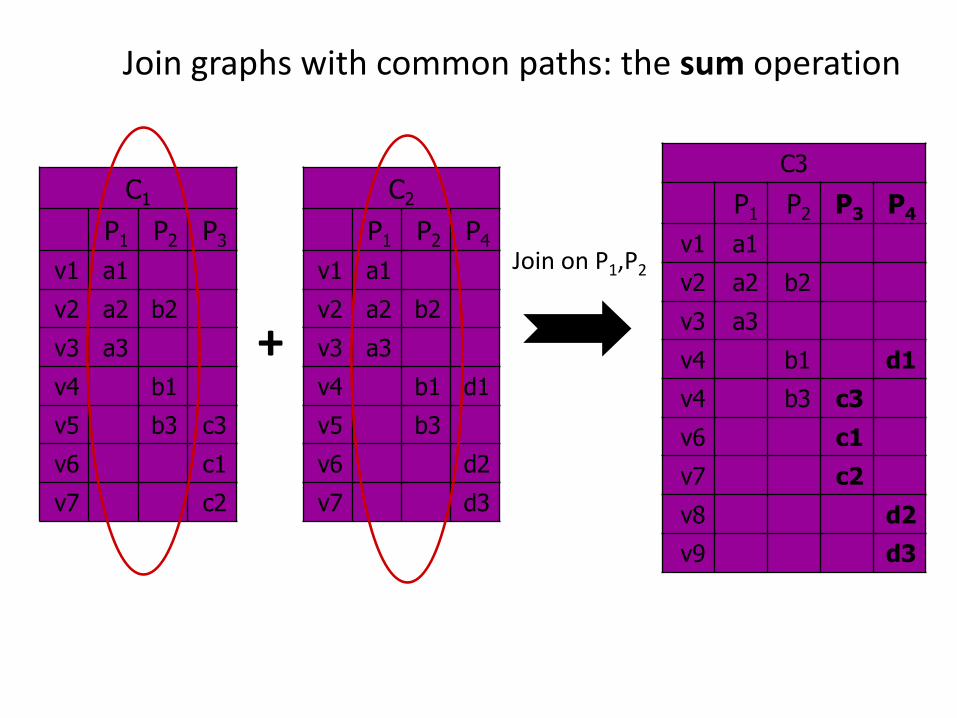
C1
P1 P2 P3
v1 a1
v2 a2 b2
v3 a3
v4 b1
v5 b3 c3
v6 c1
v7 c2
Join graphs with common paths: the sum operation
C2
P1 P2 P4
v1 a1
v2 a2 b2
v3 a3
v4 b1 d1
v5 b3
v6 d2
v7 d3
C3
P1 P2 P3 P4
v1 a1
v2 a2 b2
v3 a3
v4 b1 d1
v4 b3 c3
v6 c1
v7 c2
v8 d2
v9 d3
+
Join on P1,P2

The sum operation: how it looks on graphs
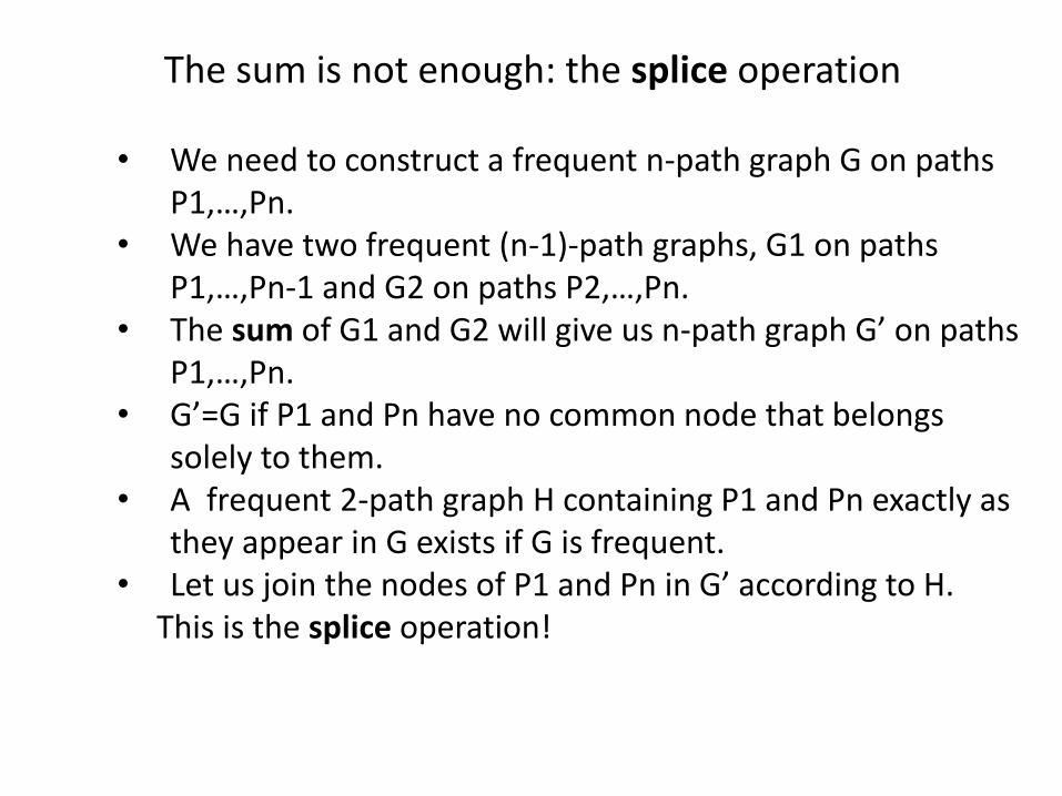
• We need to construct a frequent n-path graph G on paths P1,…,Pn.
• We have two frequent (n-1)-path graphs, G1 on paths P1,…,Pn-1 and G2 on paths P2,…,Pn.
• The sum of G1 and G2 will give us n-path graph G’ on paths P1,…,Pn.
• G’=G if P1 and Pn have no common node that belongs solely to them.
• A frequent 2-path graph H containing P1 and Pn exactly as they appear in G exists if G is frequent.
• Let us join the nodes of P1 and Pn in G’ according to H.This is the splice operation!
The sum is not enough: the splice operation
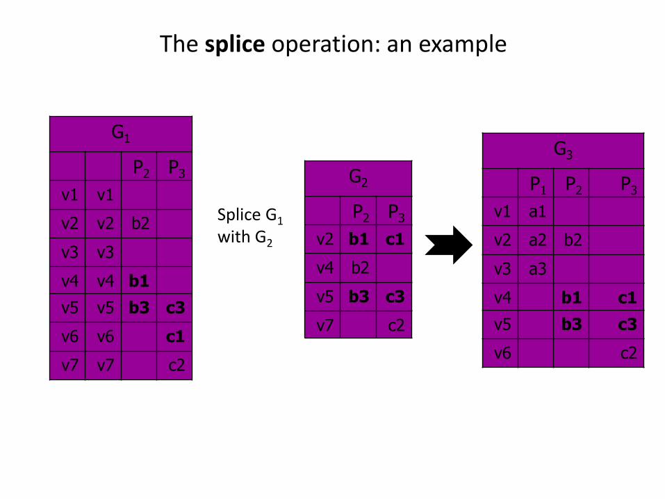
G3
P1 P2 P3
v1 a1
v2 a2 b2
v3 a3
v4 b1 c1
v5 b3 c3
v6 c2
The splice operation: an example
G1
P2 P3
v1 v1
v2 v2 b2
v3 v3
v4 v4 b1
v5 v5 b3 c3
v6 v6 c1
v7 v7 c2
G2
P2 P3
v2 b1 c1
v4 b2
v5 b3 c3
v7 c2
Splice G1
with G2
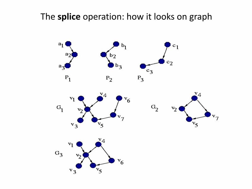
The splice operation: how it looks on graph

Labeled graphs: we mind the labels
We join only nodes that have the same labels!
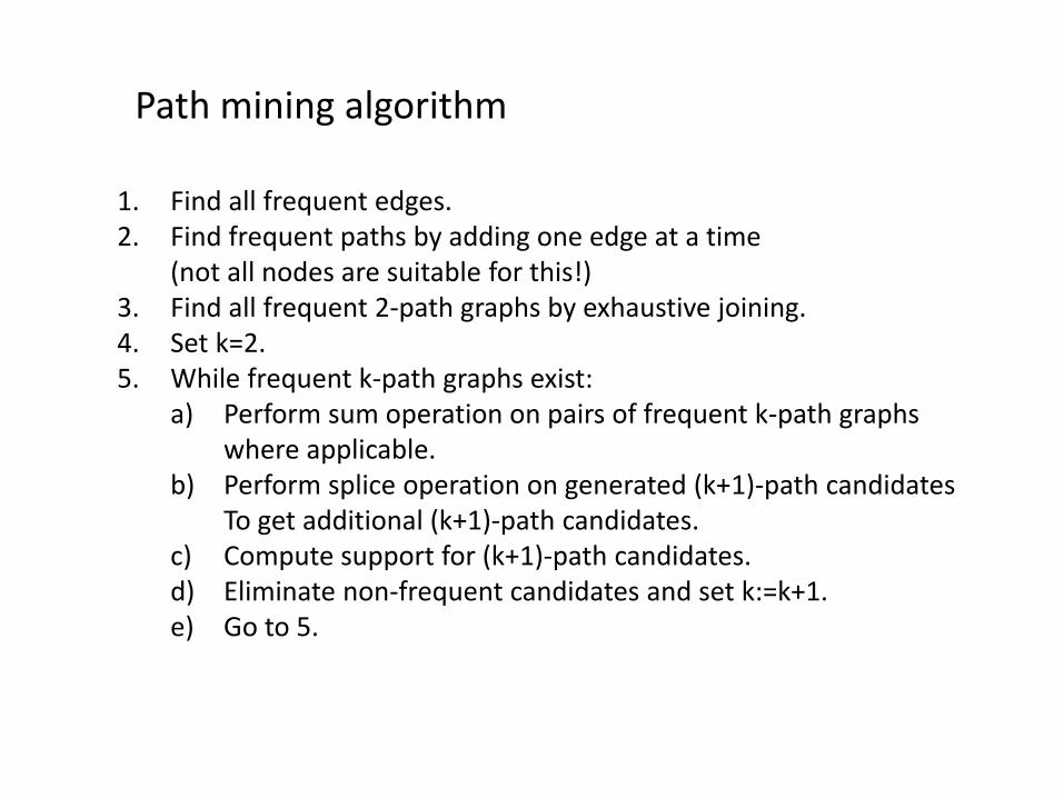
Path mining algorithm
1. Find all frequent edges.2. Find frequent paths by adding one edge at a time
(not all nodes are suitable for this!)3. Find all frequent 2-path graphs by exhaustive joining.4. Set k=2.5. While frequent k-path graphs exist:
a) Perform sum operation on pairs of frequent k-path graphswhere applicable.
b) Perform splice operation on generated (k+1)-path candidatesTo get additional (k+1)-path candidates.
c) Compute support for (k+1)-path candidates.d) Eliminate non-frequent candidates and set k:=k+1.e) Go to 5.

ComplexityExponential – as the number of frequent patterns can be exponential
on the size of the database (like any Apriori alg.)
Difficult tasks: (NP hard)1. Support computation that consists of:
a. Finding all instances of a frequent pattern in the database. (sub-graph isomorphism)
b. Computing MIS (maximum independent set size) of an instance graph.
Relatively easy tasks:1. Candidate set generation:
polynomial on the size of frequent set fromprevious iteration,
2. Elimination of isomorphic candidate patterns:graph isomorphism computation is at worstexponential on the size of a pattern, not the database.
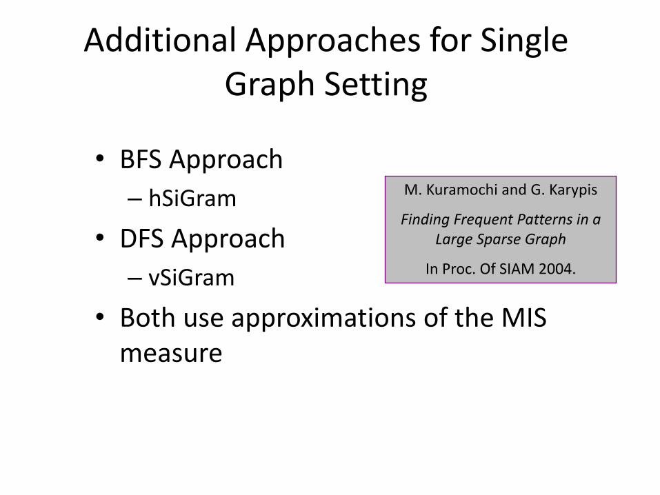
Additional Approaches for Single Graph Setting
• BFS Approach
– hSiGram
• DFS Approach
– vSiGram
• Both use approximations of the MIS measure
M. Kuramochi and G. Karypis
Finding Frequent Patterns in a Large Sparse Graph
In Proc. Of SIAM 2004.


Conclusions
• Data Mining field proved its practicality during its short lifetime with effective DM algorithms.
• Many applications in Databases, Chemistry&Biology, Networks, etc.
• Both Transaction and Single graph settings are important
• Graph Mining is: – Dealing with designing effective algorithms for mining graph datasets.– Facing many hardness problems on the way.– Fast growing field with many possibilities of evolving unseen before.
• As more and more information is stored in complicated structures, we need to develop new set of algorithms for Graph Data Mining.
Some References
[1] T. Washio A. Inokuchi and H.~Motoda, An Apriori-Based Algorithm for Mining Frequent Substructures from Graph Data, Proceedings of the 4th PKDD'00, 2000, pages 13-23.
[2] M. Kuramochi and G. Karypis, An Efficient Algorithm for Discovering Frequent Subgraphs, Tech. report, Department of Computer Science/Army HPC Research Center, 2002.
[3] N. Vanetik, E.Gudes, and S. E. Shimony, Computing Frequent Graph Patterns from Semistructured Data, Proceedings of the 2002 IEEE ICDM'02
[4] Y. Xifeng and H. Jiawei, gspan: Graph-Based Substructure Pattern Mining, Tech. report, University of Illinois at Urbana-Champaign, 2002.
[5] W. Wang J. Huan and J. Prins, Efficient Mining of Frequent Subgraphs in the Presence of Isomorphism, Proceedings of the 3rd IEEE ICDM'03 p.~549.
[6] Moti Cohen, Ehud Gudes, Diagonally Subgraphs Pattern Mining. DMKD 2004, pages 51-58, 2004
[7] D. J. Cook and L. B. Holder, Graph-Dased Data Mining, Tech. report, Department of CS Engineering, 1998.
Documents Classification:
Alternative Representation of Multilingual
Web Documents:The Graph-Based Model
Introduced in A. Schenker, H. Bunke, M. Last, A. Kandel,
Graph-Theoretic Techniques for Web Content Mining, World
Scientific, 2005
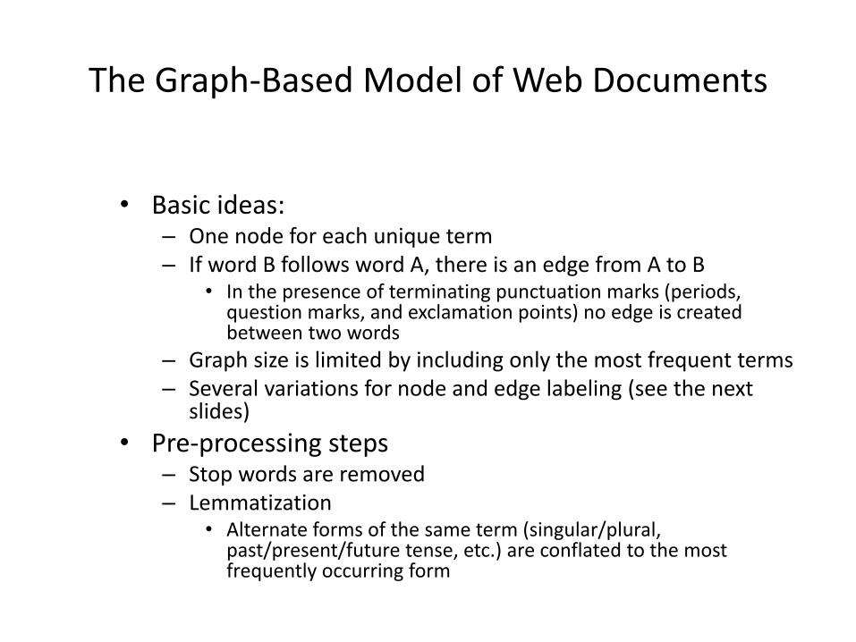
The Graph-Based Model of Web Documents
• Basic ideas:– One node for each unique term– If word B follows word A, there is an edge from A to B
• In the presence of terminating punctuation marks (periods, question marks, and exclamation points) no edge is created between two words
– Graph size is limited by including only the most frequent terms– Several variations for node and edge labeling (see the next
slides)
• Pre-processing steps– Stop words are removed– Lemmatization
• Alternate forms of the same term (singular/plural, past/present/future tense, etc.) are conflated to the most frequently occurring form
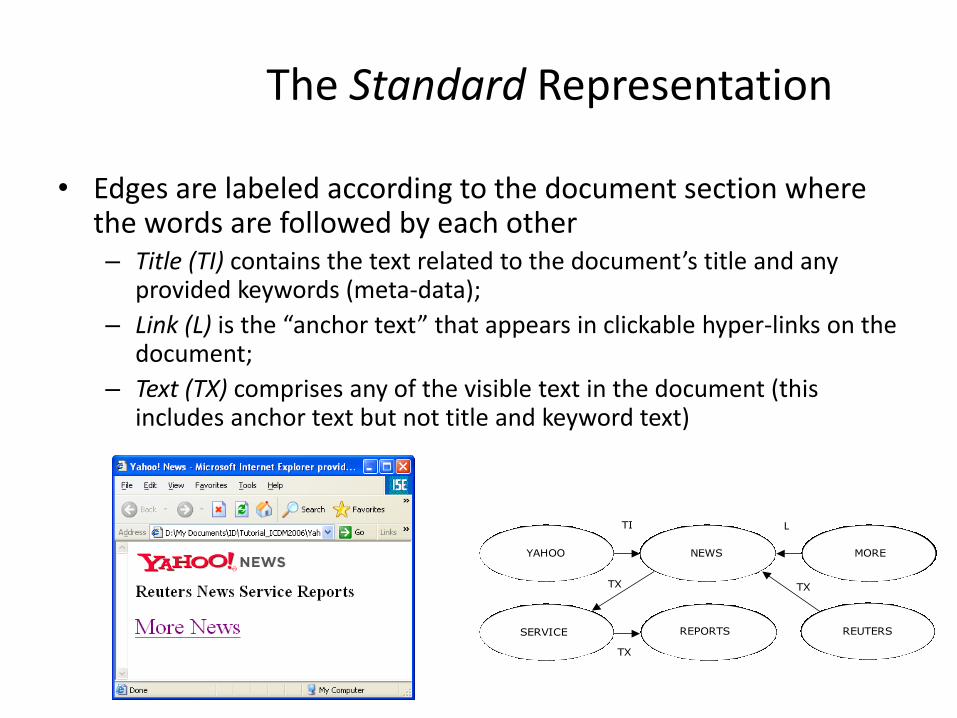
The Standard Representation
• Edges are labeled according to the document section where the words are followed by each other– Title (TI) contains the text related to the document’s title and any
provided keywords (meta-data);
– Link (L) is the “anchor text” that appears in clickable hyper-links on the document;
– Text (TX) comprises any of the visible text in the document (this includes anchor text but not title and keyword text)
YAHOO NEWS
SERVICE
MORE
REPORTS REUTERS
TI L
TX
TX
TX
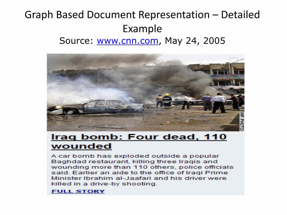
Graph Based Document Representation – Detailed Example
Source: www.cnn.com, May 24, 2005
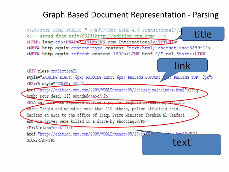
Graph Based Document Representation - Parsing
title
link
text
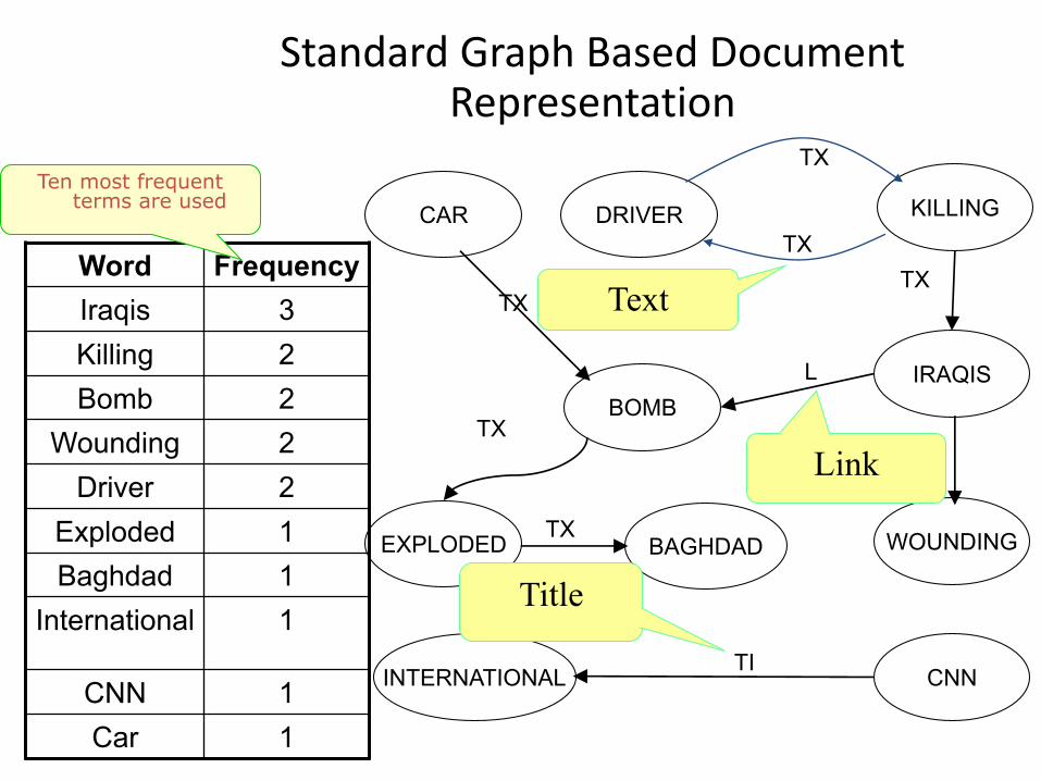
Standard Graph Based Document Representation
FrequencyWord
3Iraqis
2Killing
2Bomb
2Wounding
2Driver
1Exploded
1Baghdad
1International
1CNN
1Car
IRAQIS
CNN
KILLINGDRIVER
BOMB
EXPLODED
CAR
BAGHDAD
INTERNATIONAL
WOUNDING
TI
TX
TX
TX
TX
TX
TXTX
L
Title
Text
Link
Ten most frequent terms are used
Classification using graphs
• Basic idea:
– Mine the frequent sub-graphs, call them terms
– Use TFIDF for assigning the most characteristic terms to documents
– Use Clustering and K-nearest neighbors classification
Subgraph Extraction
• Input
– G – training set of directed, unique nodes graphs
– CRmin - Minimum Classification Rate
• Output
– Set of classification-relevant sub-graphs
• Process:
– For each class find subgraphs CR > CRmin
– Combine all sub-graphs into one set
• Basic Assumption
– Classification-Relevant Sub-Graphs are more frequent in a specific
category than in other categories

Computing the Classification Rate
• Subgraph Classification Rate:
ikikik cgISFcgSCFcgCR
• SCF (g’k(ci)) - Subgraph Class Frequency of subgraph g’k in category ci
• ISF (g’k(ci)) - Inverse Subgraph Frequency of subgraph g’k in category ci
• Classification Relevant Feature is a feature that best explains a specific
category, or frequent in this category more than in all others

k-Nearest Neighbors with GraphsAccuracy vs. Graph Size
70%
74%
78%
82%
86%
1 2 3 4 5 6 7 8 9 10
Number of Nearest Neighbors (k)
Cla
ssific
ation A
ccura
cy
Vector model (cosine) Vector model (Jaccard) Graphs (40 nodes/graph)
Graphs (70 nodes/graph) Graphs (100 nodes/graph) Graphs (150 nodes/graph)

Related Documents