Introduction to Computational Quantum ChemistryIntroduction to Computational Quantum Chemistry Lesson 8: Population analysis Martin Nov´ak & Pankaj Lochan Bora Population Analysis

Introduction to Computational Quantum Chemistry

Lesson 8: Population analysis

Martin Novak & Pankaj Lochan Bora Population Analysis October 13, 2015 1 / 30

Importance

Pictures of orbitals are informative, however numerical values aremuch easier to quantified and compared. For example σ vs π bondingin organic molecules.

What does a population analysis deliver?Determination of the distribution of electrons in a moleculeCreating orbital shapeDerivation of atomic charges and dipole ( multiple ) moments

Methods of calculationBased on the wave function ( Mulliken, NBO)Based on the electron density (Atoms in Molecules)Fitted to the electrostatic potential (CHELPG, MK)


Mulliken Population Analysis


Mulliken Population Analysis

AdvantagesMost popular methodStandard in program packages like GaussianFast and simple method for determination of electron distributionand atomic charged

DisadvantageStrong dependance of the results from the level of theory (basisset or kind of calculation)

Example: Li-charge in LiF

Population basis set q(Li,RHF) q(Li,B3LYP)Mulliken STO-3G +0.227 +0.078

6-31G +0.743 +0.5936-311G(d) +0.691 +0.558


Natural Bond Orbital Analysis


Natural Bond Orbital Analysis

Based on the theory of Natural Orbitals by Lowdin.

Two parts of the methodsNPA→ Natural population analysis to identify the populationnumbersNBO→ Analysis of the bond order based on the electronpopulation obtained by NPA

AdvantagesSmaller dependence on the basis setbetter reproducibility for different moleculesOrientates itself at the formalism for Lewis formulas


Practical task

Draw HF molecule, optimize the geometry and generate G09input.Use pop=(nbo,savenbo) for NBO or Pop=Full for MullikenAfter Pop command, add a space and type ”FormCheck”Run the calculation



Visualizing the orbitals

Open the *FChk file in AvogadroClick on Extensions→ Create SurfaceSelect ”Molecular Orbital” as surface typeChoose the MO you want to visualize and calculate


You should be able to see something like these that shows the HOMOand LUMO of HF molecules


Lesson 8: Solvation models


Solvent effects

The solvent environment influences structure, energies, spectraetcShort-range effects

Typically concentrated in the first solvation sphereExamples: h-bonds, preferential orientation near an ion

Long-range effectsPolarization


Imlicit vs. Explicit solvation

Implicit solvationDielectric continuumNo water molecules per seWavefunction of solute affected by dielectric constant of solventAt 20 °C: Water - ε = 78.4; benzene: ε = 2.3 ...

Explicit solvationSolvent molecules included (i.e. with electronic & nuclear structure)Used mainly in MM approachesMicrosolvation: only few solvent molecules placed around soluteCharge transfer with solvent can occur


Implicit Models


Basic assumptions

Solute characterized by QM wavefunctionBorn-Oppenheimer approximationOnly interactions of electrostatic originIsotropic solvent at equilibriumStatic model


Cavity

Solute is placed in a void of surrounding solvent called “cavity”Size of the cavity:

Computed using vdW radii of atoms (from UFF, for example)Taken from the electronic isodensity level (typically ˜0.001 a.u.)

The walls of cavity determine the interaction interface (SolventExcluded Surface, SES)Size of the solvent molecule determines the Solvent AccessibleSurface (SAS)


Visualizing cavity

Geomview software (in the modules)SCRF=(read) in the route section of the jobUse G03Defaults in SCRF command“geomview” in the SCRF specificationVisualize the “tesserae.off” file


Electrostatic Interactions

Self-consistent solution of solute-solvent mutual polarizationsSolute induces polarization at the interface of cavityThis polarization acts back on the solute changing its wavefunctionVarious solvation models use different schemes for evaluation ofsolvation effectsProblems arise when electrostatics do not dominate solvent-soluteinteractions


Polarizable Continuum Model (PCM)

Treats the solvent as polarizable dielectric continuumInduced surface charged represent solvent polarizationImplemented in Gaussian, GAMESS


Solvation Model “Density” (SMD)

Full solute density is used instead of partial chargesLower unsigned errors against experimental data than othermodels


COnductor-like Screening MOdel (COSMO)

Solute in virtual conductor environmentCharge q on molecular surface is lower by a factor f(ε):

q = f(ε)q∗ (1)

where f(ε) = (ε− 1)/(ε+ x); x being usually set to 0.5 or 0Implemented in Turbomole, ADF


Beyond basic models

Anisotropic liquidsConcentrated solutions


Explicit Models


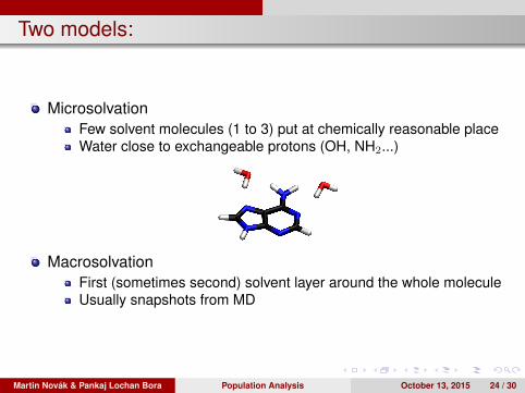
Two models:

MicrosolvationFew solvent molecules (1 to 3) put at chemically reasonable placeWater close to exchangeable protons (OH, NH2...)

MacrosolvationFirst (sometimes second) solvent layer around the whole moleculeUsually snapshots from MD


Pros & Cons

+++ Modelling of real interactions with solvent (this can be crucialfor exchangeable protons in protic solvents)- Microsolvation lacks sampling- Computationally more demanding- For macrosolvation only single point calculations - the geometryis as good as forcefield


Practical task


Reaction

Model the Cl− + CH3Br→ CH3Cl + Br−

Find the energy barrier for the reactionSelect any solvent from Gaussian library (be not concerned aboutsolubility of species or chemical relevance)Assume Sn1 and Sn2 reaction pathwaysUse “SCRF=(solvent=XY)” in the route section of the calculation


Procedure

Use B3LYP 6-31++g(d,p) methodUsage of difuse functions when dealing with anions is crucial!Use ultrafine integration gridUse Frequency calculations to be sure where on PES you areFor the scan use the distance between C and Cl as RCNegative value of step defines two atoms approaching


Module “qmutil”

Extraction of values from gaussian runs:extract-gopt-ene logfileextract-gopt-xyz logfileextract-gdrv-ene logfileextract-gdrv-xyz logfileextract-xyz-str xyzfile framenumberextract-xyz-numstr xyzfile

Values ready for plotting in your favorite software


Turbomole

Prepare job using define module (see presentation 6 for help)Setup COSMO using cosmoprep moduleSet epsilon to 78.4 and rsolv to 1.93

Leave all other values at their defaultDefine radii of atoms using “r all o” for optimized valuesOptimize all geometries


Introduction to Computational Quantum ChemistryIntroduction to Computational Quantum Chemistry Lesson 8: Population analysis Martin Nov´ak & Pankaj Lochan Bora Population Analysis

Documents