Computational and Quantum Mechanical Investigations of Oxide and Halide Perovskites using First-principles Study A dissertation Submitted for Partial Fulfilment of The Requirements for the degree of Doctor of Philosophy (Ph.D.) In Physics By NAZIA ERUM Roll No. Ph.D.-1303 Under the Kind Supervision of Prof. Dr. Muhammad Azhar Iqbal Department of Physics University of the Punjab, Lahore, Pakistan. August 2018

Welcome message from author
This document is posted to help you gain knowledge. Please leave a comment to let me know what you think about it! Share it to your friends and learn new things together.
Transcript

Computational and Quantum Mechanical
Investigations of Oxide and Halide Perovskites
using First-principles Study
A dissertation Submitted for Partial Fulfilment of
The Requirements for the degree of
Doctor of Philosophy (Ph.D.)
In
Physics
By
NAZIA ERUM
Roll No. Ph.D.-1303
Under the Kind Supervision of
Prof. Dr. Muhammad Azhar Iqbal
Department of Physics
University of the Punjab,
Lahore, Pakistan.
August 2018

İİ
CERTIFICATE
It is certified that the research work contained in this thesis has been performed by Miss Nazia
Erum, Ph.D. scholar in the subject of Physics, Roll No. Ph.D.-1303, enrolled in Fall 2013 in the
Department of Physics, University of the Punjab, Lahore, hereby declare that the matter printed in
this thesis entitled “Computational and Quantum Mechanical Investigations of Oxide and
Halide Perovskites using First-principles Study” is the result of my own original investigation,
no part of this thesis falls under plagiarism and has not been submitted as a whole or in part for
any degree or diploma at this or any other university. If found otherwise, I will be responsible for
the consequences.
Nazia Erum
Supervisor Prof. ® Dr. Muhammad Azhar Iqbal
Department of Physics,
University of the Punjab, Lahore, ______________________
Pakistan.
Chairman Dr. Mahmood-ul-Hassan
Department of Physics,
University of the Punjab, Lahore, ______________________
Pakistan.

İİİ
DEDICATIONS
I dedicate this thesis to my spiritual father, great saint HAZRAT ALLAMA ASAD NIZAMI
CHISTI SULEMANI Rehmatullahi A'laih spiritual son of Sheikh-ul-Islam wal-Muslimeen
Hazrat Baba Fareed-ud-din Masood Ganjsaker Chisti Farooqi Rehmatullahi A'laih and to my
parents who have supported me all the way since the beginning of my studies. Finally, this thesis
is dedicated to all those who believe in the richness of learning.

İꓦ
Title
Computational and Quantum Mechanical
Investigations of Oxide and Halide Perovskites
using First-principles Study

ꓦ
ABSTRACT
Fluoride and oxide perovskite structures are attracting huge interest in recent years due to their
special functionalities. In this thesis, the theoretical investigation on wide range of useful
compounds from perovskite family have been studied thoroughly for their possible
technological applications. Within the framework of Density Functional Theory (DFT),
structural, elastic, mechanical, electronic, optical, magnetic and thermodynamic properties are
studied by employing Full Potential-Linearized Augmented Plane Wave (FP-LAPW) method.
For the said investigation, the WIEN2k package is utilized.
The investigations on fluorine based strontium series of perovskites SrMF3 (M = Li, Na, K,
Rb) reveals that in these mechanically stable fluoroperovskites, brittleness and ionic behavior
are dominated which decreases from SrLiF3 to SrRbF3. Calculated energy band profiles
confirm wide and direct (Γ-Γ) bandgap. A predominant characteristic associated with cation
replacement shows that Li by Na, Na by K, and K by Rb significantly reduces the direct
bandgap in SrMF3 (M = Li, Na, K, Rb) compounds. This crucial variation is responsible for
working in different Ultra-Violet regions of the spectrum. Furthermore, from application point
of view, they could preferably be used in lens materials because they would not tolerate
birefringence that would make design of lenses difficult but also can be used in the confinement
of light for Light Emitting Devices.
The optimizations of structural parameters for rubidium based fluoroperovskite, RbHgF3 is
done with variety of approximations, which validates through comparison with available
experimental data. Energy band profile authenticates that inspected material is a narrow and
indirect energy bandgap (M–Γ) semiconductor while contour maps of electron density verifies,
mixed covalent-ionic behavior. In addition to it, optical responses show wide range of
absorption and reflection in high frequency regions.
Several elastic and mechanical parameters, reveals that protactinium based oxide series of
perovskites XPaO3 (X = K, Rb) are mechanically stable and possesses weak resistance to shear
deformation as compared with resistance to unidirectional compression while flexible and
covalent behaviors are dominated in them. The analysis of band profile through Tran–Blaha
modified Becke–Johnson (TB-mBJ) potential highlights the underestimation of bandgap with
traditional Density Functional Theory (DFT) approximation. Specific contribution of

ꓦİ
electronic states are investigated by means of total and partial density of states and it can be
evaluated that both compounds are direct bandgap (Γ–Γ) semiconductors. The study on BaMO3
(M= Pa,U) explores, type of chemical bonding with the help of variations in electron density
difference distribution that is induced due to changes of second cation. The results of electronic
properties illustrate direct bandgap (Γ-Γ) semi-conductive nature with the bandgap of 4.20 eV
and 4.01 eV for BaPaO3 and BaUO3 compounds respectively. The band gap dependent optical
properties such as complex dielectric function Ԑ (ω), optical conductivity σ (ω), refractive
index n (ω), reflectivity R (ω), and effective number of electrons (neff) via sum rules are
reported for the first time.
The investigations on KXF3 (X = V, Fe, Co, Ni) authenticates that this class of
fluoroperovskites are elastically as well as mechanically stable and anisotropic while KCoF3
is harder than rest of the compounds. The calculated spin dependent magnetoelectronic
properties in these compounds shows that exchange splitting is dominated by N-3d orbital. The
stable magnetic phase optimizations verify the experimental observations at low temperature.
The present methodology represents an influential approach to calculate the whole set of
mechanical and magneto-opto-electronic parameters, which would support to understand
various physical phenomena and empower device engineers for implementing these materials
in spintronic applications.
The pressure induced structural, elastic, mechanical, electronic, optical and thermodynamic
properties of SrLiF3, SrNaF3, SrKF3, SrRbF3, and CaLiF3 are computationally calculated for
their possible technological outcomes. All elastic and mechanical parameters are linearly
dependent on applied pressure and an increase in pressure improves tensile strength and
stiffness, on the other hand, reduces brittleness and compressibility of these cubic
fluoroperovskites. It is observed that an increase in pressure considerably improves the wide
and direct (Γ-Γ) electronic bandgap. The optical parameters of SrLiF3 and SrNaF3 shows that
all optical responses shift towards higher energy ranges which divulges that both are more
suitable for optoelectronic devices at higher pressure ranges. Consequently, our theoretical
work has been benchmarked various quantum mechanical effects, which will motivate research
scholars to done theoretical as well as experimental investigations on fluoride and oxide
perovskites that must be considered to understand and utilize these materials in fabricating
practical devices for optoelectronic, microelectronic, spintronic and piezoelectric applications.

ꓦİİ
ACKNOWLEDGEMENTS
“A man can only attain knowledge with
the help of those who possess it.
This must be understood from the very beginning.
One must learn from him who knows.”
George Gordjieft.
First and foremost, all praise to Almighty ALLAH, the most Merciful, the Compassionate, the
creator and sustainer of all the universe, who is the origin of all knowledge and wisdom, who
gave me the courage and power to accomplish this research work. Without his grace and mercy,
this work would have not been accomplished. In this universe for the guidance of human being
almighty ALLAH bestow Anbiya-Karam. By these holy souls God remove the nastiest billows
of infidelity & incredulity and illustrate his creation towards the precise way of persistent
religious conviction and last but not the least accomplished Islam by sending Hazoor Sarwar-
kainat Fakhar-mojodaat Khatam-ul-anbiya Hazrat Muhammad Mustafa (Sallala ho tala aleh
Wasalam), Subhan Allah! After Prophets, the same vocation was handed over to Saints, for
preaching & persuading Islam, for propagating Toheed & Risalaat and in spreading civilization
& social intercourse these consecrated characters completely follow Hazrat Muhammad
Mustafa (Sallala ho tala aleh Wasalam).
I offer my humblest words of thanks to Holy Prophet (Sallala ho tala aleh Wasalam), the
source of unbounded knowledge, who is forever a torch of guidance and who has guided his
“Ummah” to seek knowledge from cradle to grave, whose holy teaching inspired me to

ꓦİİİ
accomplish this research work in time. I would further like to convey my sincere gratitude to
Sheikh-ul-islam wal-Muslimeen Hazrat Baba Fareed-ud-din Masood Ganjsaker Chisti
Farooqi Rehmatullahi A'laih spiritual son of Khwaja-e-Khwajgan Hazrat Khwaja
Ghareeb Nawaz Moinuddin Chisti Ajmeri Rehmatullahi A'laih, whom trustworthy high
ranked & superb personality endow with precious services for scattering the luminosity of
Islam in the subcontinent, to point up off track Muslims the right alleyway and to incline new
muslins towards Islam. Without his special favor, this work would have not been
accomplished.
To the casual observer, a thesis may appear to be solitary work. However, to complete a report
of this magnitude requires a network of support, and I am deeply indebted to many people.
In the first place, I would like to record my gratitude to my respectable supervisor, Prof. Dr.
Muhammad Azhar Iqbal, for his dynamic supervision, advice, support, generosity from the
very early stage of this work. Above all and the most needed, he provided me unflinching
encouragement and support in various ways. His truly scientific intuition has made him as a
constant oasis of ideas in major areas of theoretical as well as experimental physics, which
exceptionally not only inspire but enrich my growth as a student, a researcher and a scientist
want to be. I am indebted to him more than he knows. I acknowledge the unwavering support
received from the Dr. Mahmood-ul-Hassan, Chairman Department of Physics, University of
Punjab, Lahore, who supported and helped me a lot in resolving many issues. This is his
dedicated support that made this work to its final end.
I especially thanks to Prof. Dr. Peter Blaha, Prof. Dr. Karlheinz Schwarz, Dr. Fabien Tran,
Dr. Andreas Troster, Leila Kalantari, Jan Doumont from Vienna University of Technology,
Institute of Materials Chemistry Austria, they directly or indirectly helped me a lot in

İX
software issues during this thesis. Next, I would also like to recognize Dr. Abed Breidi, School
of Metallurgy and Materials, University of Birmingham, United Kingdom and Dr. Songke
Feng Northwestern Polytechnical University, China for innovating my concepts in various
ways. I also thanks to Professors A. Savin, R. Dronskowski, A. J. Maeland, and G. Kresse, for
fruitful scientific communications.
The accomplishments in this work cannot be fulfilled without valuable comments provided by
various journal reviewers from Computational Material Science, Physica B, Communications
in Computational Physics, Materials Research Express, Solid State Communications, and
Chinese Physics B, they not only make me eligible to do number of effective publications but
helped me to improve thesis quality a lot.
During my years pursuing the Ph.D. at Department of Physics, University of Punjab, I have
had the pleasure of meeting many intellectual people. I am thankful to all of them who helped
me in their own way all this time. I extend sincere felicitations to all the learned staff members,
technical and non-technical staff for their courteous cooperation. I am also thankful to library
staff members, especially chief librarian for giving me opportunity to utilize digital resources
effectively. I also want to express my truthful thankfulness to members of Doctoral
Programme Coordination Committee (DPCC), University of Punjab for their assistance and
useful guidance.
Where would I be without my family? My parents deserve special mention for their inseparable
support and prayers. This thesis cannot be completed without constant cooperation and
encouragement of my lovely husband Engr. Rao Muhammad Abdullah Asadi, who
sincerely raised my intellectual pursuit, his involvement with originality has nourished my
academic maturity. His dedication, care, love and persistent confidence in me, has taken the

X
load off my shoulders. Last but not least, I express my very special thanks to my mother-in-
law, for my brothers and sisters. Hopefully this is not the end but the end of a new beginning
Insha-Allah!
Nazia Erum

Table of contents
Xİ
TABLE OF CONTENTS Page
TITLE PAGE Ι
CERTIFICATE ΙΙ
DEDICATIONS ΙΙΙ
ABSTRACT V
ACKNOWLEDGMENTS VΙΙ
TABLE OF CONTENTS XΙ
LIST OF TABLES XIX
LIST OF FIGURES XXΙV
LIST OF SYMBOLS AND ABBREVIATIONS XXXVΙΙ
Chapter 1 1
Introduction 1
1.1 Overview 1
1.2 The driving forces 2
1.3 Scope and objective 4
1.3.1 Quantum mechanical investigation 4
1.3.2 First principles studies 6
1.3.3 Computational analysis 7
1.4 Perovskites 8
1.5 Crystallographic details of perovskite structures 8
1.5.1 Tolerance factor criteria for perovskites 11
1.5.2 Types of perovskites 12
1.6 Aim of the research 15
1.7 Outline of thesis 16
Chapter 2 18
Perovskite materials: From synthesis to applications 18
2.1 Overview 18
2.2 Synthesis methods for perovskite materials 19

Table of contents
Xİİ
2.2.1 Conventional inorganic solid-state synthesis 20
2.2.2 Solution-based synthesis methods 20
2.3 Prediction methods for structural properties of perovskites 21
2.4 Physical characteristics of perovskites 23
2.5 Band chemistry of perovskites 24
2.6 From insulating to superconducting perovskites 25
2.7 Magnetism and electronic correlations in perovskites 29
2.8 Thermodynamic valence stability in transition metal based perovskites 33
2.9 Properties of perovskites 34
2.9.1 Property based tentative classification of perovskites 36
2.9.2 Opto-electronic properties 36
2.9.3 Dielectric properties 38
2.9.4 Piezoelectricity 40
2.9.5 Multiferroicity 42
2.9.6 Electronic conductivity 45
2.9.7 The Seebeck coefficient 48
2.9.8 Polarons 48
2.9.9 Thermal expansion 49
2.10 Application of perovskites 50
Chapter 3 55
Literature Review 55
3.1 Overview 55
3.2 Background of materials 55
3.3 Structural properties-Previous research 57
3.4 Optoelectronic properties-Previous research 59
3.5 Elastic and mechanical properties-Previous research 62
3.6 Magnetic properties-Previous research 64
3.7 Thermodynamic properties-Previous research 70
3.8 Conclusion 72
Chapter 4 73
Theory and Computational details 73

Table of contents
Xİİİ
4.1 Introduction 73
4.2 Many body problems and Schrodinger wave equation 74
4.3 The Basic Methods of Electronic Structure 77
4.4 The Density Functional Theory (DFT) 80
4.5 Hohenberg-Kohn Theorems and Kohn Sham Equations 83
4.6 The Exchange and Correlation approximations 88
4.6.1 The Local Density approximation (LDA) 88
4.6.2 The Generalized Gradient approximation (GGA) 90
4.6.3 The modified Becke–Johnson (mBJ) potential 93
4.7 Methods for solution of Kohn Sham Equations 95
4.8 Full-Potential Linearized Augmented Plane Wave Method (FP-LAPW) 96
4.9 Simulation techniques 98
4.9.1 The WIEN2k Package 100
4.10 Applications of Density functional theory (DFT) 102
Chapter 5: Results and discussion Ι; 106
Elastic, and optoelectronic investigation of SrMF3 (M = Li, Na, K, Rb) and RbHgF3
fluoroperovskites 106
5.1 Introduction 106
5.2 Structural, elastic and mechanical properties of SrMF3 (M = Li, Na, K, Rb) 106
5.2.1 Structural properties 107
5.2.2 Elastic properties 109
5.2.3 Mechanical behavior 110
5.2.3.1 Elastic moduli calculations 110
5.2.3.2 Cauchy’s pressure and shear constant calculations 111
5.2.3.3 Poisson’s ratio and elastic anisotropy calculations 112
5.2.3.4 Melting temperature Tm and Kleinman’s parameter calculations 113
5.2.3.5 Lame’s constant calculations 114
5.3 Opto-electronic investigation of SrMF3 (M = Li, Na, K, Rb) 120
5.3.1 Electronic properties 120
5.3.1.1 Band structure calculations 120

Table of contents
Xİꓦ
5.3.1.2 Density of States (DOS) calculations 121
5.3.1.3 Electron density contour calculations 122
5.3.2 Optical parameters 122
5.3.2.1 Complex dielectric constant calculations 123
5.3.2.2 Optical conductivity and energy loss calculations 124
5.3.2.3 Sum rules calculation via neff 125
5.4 Opto-electronic investigation of RbHgF3 for low birefringent lens materials 149
5.4.1 Structural properties 149
5.4.2 Electronic Properties 150
5.4.2.1 Band structure calculations 150
5.4.2.2 Density of States (DOS) calculations 151
5.4.2.3 Electron density contour calculations 151
5.4.3 Optical properties 152
5.4.3.1 Complex dielectric constant calculations 152
5.4.3.2 Absorption coefficient calculations 153
5.4.3.3 Optical reflectivity calculations 153
5.5 Conclusion 166
Chapter 6: Results and discussion ΙΙ; 168
Investigation of mechanical and optoelectronic behavior of actinoid based oxide
Perovskites 168
6.1 Introduction 168
6.2 Mechanical and optoelectronic study of XPaO3 (X= K, Rb) 169
6.2.1 Structural properties 169
6.2.2 Elastic constant calculations 171
6.2.3 Mechanical parameters 172
6.2.3.1 Elastic moduli calculations 172
6.2.3.2 Cauchy’s pressure and Poisson’s ratio calculations 173
6.2.3.3 Shear constant and elastic anisotropy calculations 173
6.2.3.4 Lame’s constant calculations 174
6.2.3.5 Melting temperature calculations 174

Table of contents
Xꓦ
6.2.4 Electronic behavior 175
6.2.4.1 Band structure calculations 175
6.2.4.2 Density of States (DOS) calculations 175
6.2.4.3 Electron density contour calculations 176
6.2.5 Optical characteristics 176
6.2.5.1 Complex dielectric constant calculations 176
6.2.5.2 Optical conductivity and energy loss calculations 178
6.2.5.3 Refractive index and reflectivity calculations 178
6.2.5.4 Absorption coefficient calculations 179
6.2.5.5 Sum rules calculation via neff 179
6.3 Ab initio study of high dielectric constant BaMO3 (M=Pa, U) oxide perovskite 206
6.3.1 Structural parameters 206
6.3.2 Electronic behavior 208
6.3.2.1 Band structure calculations 208
6.3.2.2 Density of States (DOS) calculations 209
6.3.2.3 Electron density Calculations 209
6.3.3 Optical characteristics 209
6.3.3.1 Complex dielectric constant calculations 210
6.3.3.2 Optical conductivity calculations 210
6.3.3.3 Refractive index and reflectivity calculations 211
6.3.3.4 Sum rules calculation via neff 211
6.4 Conclusion 232
Chapter 7: Results and discussion ΙΙΙ; 234
Band profiles and magneto-optic properties of KXF3 (X= V,Fe,Co,Ni) 234
7.1 Introduction 234
7.2 Structural stability 235
7.2.1 Analytical calculations of lattice constants 236
7.2.2 Tolerance factor calculations 237
7.3 Elastic properties 237
7.3.1 Calculation of elastic constants 237

Table of contents
Xꓦİ
7.4 Mechanical properties 238
7.4.1 Calculation of elastic moduli 239
7.4.2 Calculation of Cauchy’s pressure, B/G and Poisson’s ratio 240
7.4.3 Calculation of shear constant and elastic anisotropy 240
7.4.4 Calculation of Kleinman’s parameter and Lame’s constant 241
7.5 Thermal properties (Calculation of the Debye temperature) 242
7.6 Electronic and magnetic properties 243
7.6.1 Spin-dependent band structure calculations 244
7.6.2 Spin-dependent Density of States (DOS) calculations 244
7.6.3 Spin-dependent electron density calculations 245
7.6.4 Calculation of magnetic properties 245
7.7 Optical properties 246
7.7.1 Calculation of complex dielectric function 246
7.7.2 Calculation of energy loss function 248
7.7.3 Calculation optical conductivity 248
7.7.4 Calculation of absorption coefficient 248
7.7.5 Calculation of reflectivity 249
7.7.6 Calculation of refractive index 249
7.7.7 Calculation of sum rule via neff 250
7.8 Conclusion 277
Chapter 8: Results and discussion ΙV; 278
Effect of pressure variation on strontium and calcium based fluoroperovskites 278
8.1 Introduction 278
8.2 Background of investigation 279
8.3 Pressure variation on physical properties of SrLiF3 281
8.3.1 Pressure variation on structural properties 282
8.3.2 Pressure variation on electronic properties 283
8.3.3 Pressure variation on elastic properties 285
8.3.4 Pressure variation on mechanical properties 287
8.3.5 Thermodynamic properties 289

Table of contents
Xꓦİİ
8.3.5.1 The Quasi-harmonic Debye model 289
8.3.5.2 Pressure and temperature variation on thermodynamic properties 291
8.3.6 Pressure variation on optical properties 292
8.4 Effect of pressure variation on physical properties of SrNaF3 318
8.4.1 Pressure variation on structural properties 318
8.4.2 Pressure variation on electronic properties 319
8.4.3 Pressure variation on elastic and mechanical properties 321
8.4.4 Pressure and temperature variation on thermodynamic properties 324
8.4.5 Effect of pressure variation on optical properties 326
8.5 Pressure variation on physical properties of SrKF3 352
8.5.1 Pressure variation on structural properties 352
8.5.2 Pressure variation on electronic properties 353
8.5.3 Pressure variation on elastic properties 354
8.5.4 Pressure variation on mechanical properties 356
8.5.5 Pressure variation on Debye temperature (θD) 357
8.5.6 Pressure and temperature variations on thermodynamic properties 359
8.6 Pressure variation on physical properties of SrRbF3 377
8.6.1 Pressure variation on structural properties 377
8.6.2 Pressure variation on elastic properties 378
8.6.3 Pressure variation on mechanical properties 379
8.6.4 Pressure variation on Debye temperature (θD) 380
8.6.5 Pressure and temperature variations on thermodynamic properties 380
8.7 Pressure variation on physical properties of CaLiF3 396
8.7.1 Pressure variation on structural properties 396
8.7.2 Pressure variation on elastic properties 397
8.7.3 Pressure variation on mechanical properties 398
8.7.4 Pressure variation on Debye temperature (θD) 399
8.7.5 Pressure and temperature variations on thermodynamic properties 399
8.8 Conclusion 413
Chapter 9 417
Conclusions and future work 417
Table of contents
Xꓦİİİ
9.1 Conclusions 417
9.2 Mechanical and opto-electronic properties of Perovskites 418
9.3 Magneto-opto-electronic properties of fluoroperovskites 420
9.4 Pressure and temperature dependent physical aspects of fluoroperovskites 421
9.5 Future work plan 424
REFERENCES 426
LIST OF PUBLICATIONS 462

List of Tables
XİX
LIST OF TABLES
Page
Table 1.1: Some perovskite, their tolerance factor and structures. 14
Table 2.1: Applications of perovskites along with respective properties. 54
Table 5.1: Comparison of calculated equilibrium lattice constants (ao), ground state
energies (Eo) and bulk modulus (Bo) with experimental and other theoretical
values of SrMF3 (X = Li, Na, K and Rb) compounds. 117
Table 5.2: Bond-lengths of SrMF3 (X= Li, Na, K, Rb) compounds. 117
Table 5.3: Calculated values of elastic constants C11, C12, C44, for SrMF3 (X = Li, Na, K
and Rb) compounds. 118
Table 5.4: Calculated values of Bulk modulus B0, Voigt’s shear modulus GV, Reuss’s
shear modulus GR, Hill’s shear modulus GH, Young’s modulus Y, and Pugh’s
index of ductility Bo/GH. 118
Table 5.5: Calculated values of Shear constant(𝐶′), Cauchy pressure (𝐶′′), Poisson’s
ratio (ѵ), Anisotropy constant (A), Kleinman parameter (ξ), Lame’s
coefficients (λ and μ), and Melting temperature (Tm). 119
Table 5.6: Band gap of SrMF3 (M = Li, Na, K, Rb) at different symmetry points
compared with experimental and other theoretical results. 148
Table 5.5: Comparison of Present calculation with previous experimental and theoretical
values for lattice constants (ao), ground state energies (Eo), bulk modulus (Bo)
and its pressure derivative (Bp) of RbHgF3 compound. 165
Table 6.1: Comparisons of calculated values of bond length, equilibrium lattice constant
(ao in Ǻ), ground state energy (Eo in RY), bulk modulus (Boin GPa) and its
pressure derivative (BP) with experimental and other theoretical results for
XPaO3 (X = K, Rb) compounds. 201
Table 6.2: Calculated values of tolerance factor for XPaO3 (X = K, Rb). 202
Table 6.3: Calculated values of elastic constants C11, C12, C44, for XPaO3 (X = K, Rb)
compounds. 202
Table 6.4: Calculated values of Bulk modulus B0, Reuss’s shear modulus GR, Voigt’s
shear modulus GV, Hill’s shear modulus GH, Young’s modulus Y and Pugh’s
index of ductility Bo/GH. 203

List of Tables
XX
Table 6.5: Calculated values of Shear constant (C′), Cauchy pressure (C′′), Lame’s
coefficients (λ and μ), Anisotropy constant (A in GPa) and Poisson’s ratio
(ѵ in GPa) and the melting temperature (Tm in K) for XPaO3 (X= K, Rb)
compounds. 204
Table 6.6: Band gap comparison of XPaO3 (X = K, Rb) at different symmetry points. 205
Table 6.7: Comparison of calculated equilibrium lattice constants ao (in Ǻ), ground state
energies Eo (in Ry), bulk modulus Bo (in GPa), its pressure derivative BP (in
GPa), and bond lengths with experimental and other theoretical values of
BaXO3 (X = Pa, U) compounds. 230
Table 6.8: Calculated tolerance factor for BaXO3 (X = Pa, U). 231
Table 6.9: Band gap comparison of BaXO3 (X = Pa, U) at different symmetry points. 231
Table 7.1: Comparison of experimental and calculated values of equilibrium lattice
constants (ao in Ǻ), ground state energies (Eo in Ry), bulk modulus (Bo in GPa)
and its pressure derivative (BP), and bond lengths of KXF3 (X = V,Fe,Co,Ni)
compounds. 271
Table 7.2: Calculated tolerance factor for KXF3 (X = V,Fe,Co,Ni) compounds. 272
Table 7.3: Calculated values of elastic constants (C11, C12 and C44 in GPa), for KXF3
(X = V,Fe,Co,Ni) compounds. 272
Table 7.4: Calculated values of Bulk modulus (B0 in GPa), Young’s modulus (Y in GPa),
Voigt’s shear modulus (GV in GPa), Reuss’s shear modulus (GR in GPa), and
Hill’s shear modulus (GH in GPa) for KXF3 (X = V,Fe,Co,Ni) compounds. 273
Table 7.5: Calculated values of B/G ratio, Shear constant (C’), Cauchy pressure (C’’),
Lame’s coefficients (λ and μ), Kleinman parameter (ξ in GPa), Anisotropy
constant (A in GPa) and Poisson’s ratio (ѵ in GPa) for KXF3
(X = V,Fe,Co,Ni) compounds. 274
Table 7.6: Comparison of experimental and calculated values of longitudinal (υl in Km/s),
transverse (υt in Km/s), average sound velocity (υm in Km/s), Debye
temperature (θD in K) and the melting temperature (TMelt in K) for KXF3 (X =
V,Fe,Co,Ni) compounds. 275
Table 7.7: Comparison of calculated interstitial (minst), local and total magnetic moment
(MT) in μB of KXF3 (X= V,Fe,Co,Ni) compounds with available
experimental and other theoretical data. 276

List of Tables
XXİ
Table 8.1: Comparison of the present calculation with the previous experimental and
theoretical values for the lattice constants (ao), ground state energies (Eo), bulk
modulus (Bo) and its pressure derivative (B′) at ambient pressure of SrLiF3
compound. 315
Table 8.2: Comparison of previous and calculated values of Pressure (P in GPa),
Energies (E in Ry), Volume of unit cell (V in (a.u.)3), Energy Gap (eV), and
Bond length (dSr-F, dLi-F). 315
Table 8.3: Calculated values of elastic constants (C11, C12, C44) of SrLiF3 at pressure
from 0-50 GPa. 316
Table 8.4: Derived elastic constants characterizing mechanical stability (Equations
8.1-8.3) of SrLiF3 at pressure from 0-50 GPa. 316
Table 8.5: Calculated values of elastic moduli Bulk modulus (B0), Voigt’s shear
modulus (GV), Reuss’s shear modulus (GR) and Hill’s shear modulus
(GH), and Young’s modulus (Y) of SrLiF3 at pressure from 0-50 GPa. 317
Table 8.6: Calculated values of Shear constant (C’), Cauchy pressure (C’’), Poisson’s
ratio (ѵ) Anisotropy constant (A), Kleinman parameter (ξ), and melting
temperature (Tm) of SrLiF3 at pressure from 0-50 GPa. 317
Table 8.7: Comparison of the present calculation with the previous experimental and
theoretical values for the lattice constants (ao), ground state energies (Eo),
bulk modulus (Bo) and its pressure derivative (B′) at ambient pressure of
SrNaF3 compound. 349
Table 8.8: Comparison of previous and calculated values of Pressure (P in GPa),
Energies (E in Ry), Volume of unit cell (V in (a.u.)3), Energy Gap (eV), and
Bond length (dSr-F, dNa-F). 349
Table 8.9: Calculated values of elastic constants (C11, C12, C44), of SrNaF3 at pressure
from 0-25 GPa. 350
Table 8.10: Calculated values of Bulk modulus (B0), Voigt’s shear modulus (GV),
Reuss’s shear modulus (GR) and Hill’s shear modulus (GH), Young’s
modulus (Y), and B/G ratio, of SrNaF3 at pressure from 0-25 GPa. 350
Table 8.11: Calculated values of Poisson’s ratio (ѵ), Cauchy pressure (C’’), Anisotropy
constant (A), Kleinman parameter (ξ), and melting temperature (Tm) of
SrNaF3 at pressure from 0-25 GPa. 351
Table 8.12: Derived elastic constants characterizing mechanical stability (Equations
8.33-8.35) of SrNaF3 at pressure from 0-25 GPa. 351

List of Tables
XXİİ
Table 8.13: Comparison of the present calculation with the previous experimental and
theoretical values for the lattice constants (ao), ground state energies (Eo),
bulk modulus (Bo) and its pressure derivative (B′) at ambient pressure of
SrKF3 compound. 373
Table 8.14: Comparison of previous and calculated values of Pressure (P in GPa),
Energies (E in Ry), Volume of unit cell (V in (a.u.)3), Energy Gap (eV), and
Bond length (dSr-F, dK-F). 373
Table 8.15: Calculated values of elastic constants (C11, C12, C44) of SrKF3 at pressure
from 0-25 GPa. 374
Table 8.16: Calculated values of Bulk modulus (B0), Voigt’s shear modulus (GV),
Reuss’s shear modulus (GR) and Hill’s shear modulus (GH), Young’s
modulus (Y), and B/G ratio of SrKF3 at pressure from 0-25 GPa. 374
Table 8.17: Calculated values of Poisson’s ratio (ѵ), Cauchy pressure (C’’), Anisotropy
constant (A), Kleinman parameter (ξ), melting temperature (Tm),
longitudinal (υl in m/s), transverse (υt in m/s), average sound velocity (υm in
m/s), and Debye temperature (θD in K) of SrKF3 at pressure from 0-25 GPa. 375
Table 8.18: Derived elastic constants characterizing mechanical stability (equation 8.36-
8.38) of SrKF3 at pressure from 0-25 GPa. 376
Table 8.19: Comparison of the present calculation with the previous experimental and
theoretical values for the lattice constants (ao), ground state energies (Eo),
bulk modulus (Bo) and its pressure derivative (B′) at ambient pressure for
SrRbF3 compound. 393
Table 8.20: Comparison of previous and calculated values of Pressure (P in GPa),
Energies (E in Ry), Volume of unit cell (V in (a.u.)3) and Bond length
(dSr-F, dRb-F) of SrRbF3 compound. 393
Table 8.21: Calculated values of elastic constants (C11, C12, C44) of SrRbF3 at pressure
from 0-25 GPa. 394
Table 8.22: Calculated values of derived elastic constants characterizing mechanical
stability of SrRbF3 at pressure from 0-25 GPa. 394
Table 8.23: Calculated values of Bulk modulus (B0), Voigt’s shear modulus (GV),
Reuss’s shear modulus (GR) Hill’s shear modulus (GH), Young’s modulus
(Y), and B/G ratio of SrRbF3 at pressure from 0-25 GPa. 395

List of Tables
XXİİİ
Table 8.24: Calculated values of Poisson’s ratio (ѵ), Cauchy pressure (C’’), Anisotropy
constant (A), Kleinman parameter (ξ), melting temperature (Tm),
longitudinal (υl in m/s), transverse (υt in m/s), average sound velocity (υm in
m/s), and Debye temperature (θD in K) of SrRbF3 at pressure from 0-25 GPa. 395
Table 8.25: Comparison of the present calculation with the previous experimental and
theoretical values for the lattice constants (ao), ground state energies (Eo),
bulk modulus (Bo) and its pressure derivative (B′) at ambient pressure of
CaLiF3 compound. 410
Table 8.26: Comparison of previous and calculated values of Pressure (P in GPa),
Energies (E in Ry), Volume of unit cell (V in (a.u.)3) and Bond length
(dCa-F, dLi-F) of CaLiF3 compound. 410
Table 8.27: Calculated values of elastic constants (C11, C12, C44) of CaLiF3 at pressure
from 0-50 GPa. 411
Table 8.28: Calculated values of derived elastic constants characterizing mechanical
stability of CaLiF3 at pressure from 0-50 GPa. 411
Table 8.29: Calculated values of Bulk modulus (B0), Voigt’s shear modulus (GV),
Reuss’s shear modulus (GR), Hill’s shear modulus (GH), Young’s
modulus (Y), and B/G ratio, of CaLiF3 at pressure from 0-50 GPa. 412
Table 8.30: Calculated values of Poisson’s ratio (ѵ), Anisotropy constant (A), Kleinman
parameter (ξ), melting temperature (Tm) longitudinal (υl in m/s), transverse
(υt in m/s), average sound velocity (υm in m/s), and Debye temperature
(θD in K) of CaLiF3 at pressure from 0-50 GPa. 412

List of Figures
XXİꓦ
LIST OF FIGURES Page
Figure 1.1: Schematic diagram showing correlation between First principles study,Quantum
mechanical investigation and computational analysis. 9
Figure 1.2: Comparison between fundamental quantum mechanics and technology of the
classical world. 9
Figure 1.3: Schematic representation showing journey of quantum mechanical
Investigation for evaluating physical properties of material. 10
Figure 1.4: A generic perovskite structure of the form ABX3. Note however that the two
structures are equivalent – the left-hand structure is drawn so that atom B is at
the <0,0,0> position while the right-hand structure is drawn so that atom
(or molecule) A is at the <0,0,0> position. Also note that the lines are a guide
to represent crystal orientation rather than bonding patterns. 10
Figure 1.5: The ideal ABX3 perovskite structure showing the octahedral and icosahedral
(12-fold) coordination of the B and A-site cations, respectively. 13
Figure 1.6: Illustration of the simple cubic perovskite unit along one of the main unit cell
axes in (a) an ideal cubic perovskite with a larger A-site cation and (b) a
smaller A site cation. 14
Figure 2.1: Perovskite mineral species (CaTiO3) along with Lev Aleksevich von
Perovski. 19
Figure 2.2: Structure and morphology of perovskite mineral. 23
Figure 2.3: Schematic illustration of the band gap in solid materials. 27
Figure 2.4: A band gap diagram showing the approximate band energies in ABO3 that
from the density of states (DOS) in a perovskite. 28
Figure 2.5: A band gap diagram showing the different sizes of band gaps for conductors,
semiconductors, and insulators. 28
Figure 2.6: Block diagram breakdown of chemical and physical properties of matter. 35
Figure 2.7: Schematic illustration for the phenomenon of piezoelectric effect. 42
Figure 2.8: Multiferroics combine the properties of ferroelectrics and ferromagnets. 46
Figure 2.9: Block diagram illustration of perovskites multiferroics 46
Figure 2.10: The multiferroics totem; illustrating the three main ferroic orders with their
respective fields and crossed interactions. 47
List of Figures
XXꓦ
Figure 2.11: Conditions required for ferroelectricity (polarization) and ferromagnetism
(unpaired electron spin motion). 47
Figure 2.12: Various applications of perovskites quantum dot, nanowire and nanosheet. 53
Figure 3.1: Illustration of the different orbitals that overlap with a) strong eg-pσ and b)
t2g-pπ overlaps between two transition metals with dn configuration and an
oxygen, i.e., the M-O-M bonds. 68
Figure 3.2: Emergence of the novel interface magnetic state at the heterointerfaces of
LSMO/BFO. (a) Novel interfacial magnetic state in the LSMO/BFO
heterostructure (b) Evolution of the interface magnetism and exchange bias
coupling with temperature. The vertical guiding line indicates the blocking
temperature of the exchange bias coupling and the magnetic transition
temperature of the interface magnetic state. 69
Figure 3.3: A general schematic illustration for calculating thermodynamic properties. 71
Figure 4.1: Block diagram representation of various theoretical methods. 75
Figure 4.2: Schematic chemistry of atoms and molecules in solids. 78
Figure 4.3: The evolution and classification of quantum mechanical methods. 81
Figure 4.4: Schematic presentation of Quantum methods. 82
Figure 4.5: A schematic representation of the relationship between the "real" many body
system (left hand side) and the non-interacting system of Kohn Sham density
functional theory (right hand side). 82
Figure 4.6: Schematic description of the SCF cyclic procedure in solving the
Kohn-Sham equations. 87
Figure 4.7: Partitioning of the unit cell into atomic spheres (I) and an interstitial
region (II). 99
Figure 4.8: The unit cell divided into muffin-tin region and interstitial region. 99
Figure 4.9: Flow chart of WIEN2k code SCF cycle in single mode and in parallel
Mode. 102
Figure 5.1: Crystal structures of SrMF3, Where M = Li, Na, K, and Rb (Sr+2: Blue, M+1:
Green, F-1 : Red). 115

List of Figures
XXꓦİ
Figure 5.2: Lattice constants versus change in bond lengths between M and F of SrMF3
(M = Li, Na, K, Rb). 116
Figure 5.3: Melting temperature Tm (K) Vs Klienmann parameter ξ (GPa). 116
Figure 5.4: The mBJ-electronic band dispersion curves for SrLiF3. 126
Figure 5.5: The mBJ-electronic band dispersion curves for SrNaF3. 127
Figure 5.6: The mBJ-electronic band dispersion curves for SrKF3. 128
Figure 5.7: The mBJ-electronic band dispersion curves for SrRbF3. 129
Figure 5.8: The Density of States for SrLiF3 by mBJ potential. 130
Figure 5.9: The Density of States for SrNaF3 by mBJ potential. 131
Figure 5.10: The Density of States for SrKF3 by mBJ potential. 132
Figure 5.11: The Density of States for SrRbF3 by mBJ potential. 133
Figure 5.12 (a): Calculated mBJ total two and three-dimensional electronic charge
densities for SrLiF3 in (100) plane. 134
Figure 5.12 (b): Calculated mBJ total two and three-dimensional electronic charge
densities for SrNaF3 in (100) plane. 135
Figure 5.12 (c): Calculated mBJ total two and three-dimensional electronic charge
densities for SrKF3 in (100) plane. 136
Figure 5.12 (d): Calculated mBJ total two and three-dimensional electronic charge
densities for SrRbF3 in (100) plane. 137
Figure 5.13 (a): Calculated mBJ total two and three-dimensional electronic charge
densities for SrLiF3 in (110) plane. 138
Figure 5.13 (b): Calculated mBJ total two and three-dimensional electronic charge
densities for SrNaF3 in (110) plane. 139
Figure 5.13 (c): Calculated mBJ total two and three-dimensional electronic charge
densities for SrKF3 in (110) plane. 140
Figure 5.13 (d): Calculated mBJ total two and three-dimensional electronic charge
densities for SrRbF3 in (110) plane. 141

List of Figures
XXꓦİİ
Figure 5.14: Total two-dimensional electron density plots in (110) plane for (a) SrLiF3
, (b) SrNaF3, (c) SrKF3, (d) SrRbF3. 142
Figure 5.15 (a): Calculated imaginary part Ԑ2 (ω) of the dielectric function for the SrMF3
(M=Li, Na, K, Rb) compounds. 143
Figure 5.15 (b): Calculated real part Ԑ1 (ω) of the dielectric function for the SrMF3
(M=Li, Na, K, Rb) compounds. 144
Figure 5.15 (c): Calculated energy loss function L (ω) for SrMF3 (M=Li,Na,K,Rb
compounds. 145
Figure 5.15 (d): Calculated conductivity σ (ω) for SrMF3 (M= Li, Na, K, Rb)
compounds. 146
Figure 5.15 (e): Calculated sum rule for SrMF3 (Li,Na,K,Rb) compounds. 147
Figure 5.16: Cubic crystal structure of RbHgF3. 154
Figure 5.17: Variation of total energy as a function of unit cell volume for RbHgF3. 155
Figure 5.18: Comparison of band structures in high symmetry directions with mBJ and
PBE-GGA schemes for RbHgF3. 156
Figure 5.19: The Density of States for RbHgF3 by mBJ potential. 157
Figure 5.20 (a): Calculated mBJ total two and three-dimensional electronic charge
densities in (100) plane for RbHgF3. 158
Figure 5.20 (b): Calculated mBJ total two and three-dimensional electronic charge
densities in (110) plane for RbHgF3. 159
Figure 5.21 (a): Total two-dimensional electron density plots in the (100) plane for
RbHgF3. 160
Figure 5.21 (b): Total two-dimensional electron density plots in the (110) plane for
RbHgF3. 160
Figure 5.22 (a): Calculated imaginary part Ԑ2(ω) of the dielectric function for RbHgF3
compound. 161
Figure 5.22 (b): Calculated real part Ԑ1(ω) of the dielectric function for RbHgF3
compound. 162

List of Figures
XXꓦİİİ
Figure 5.22 (c): Calculated absorption coefficient α (ω) of dielectric function for
RbHgF3 compound. 163
Figure 5.22 (d): Reflectivity R (ω) as a function of energy for RbHgF3 compound. 164
Figure 6.1 (a): Cubic crystal structure of KPaO3 181
Figure 6.1 (b): Cubic crystal structure of RbPaO3 182
Figure 6.2 (a): Variations of total energy (E, in Ry) with unit cell volume (V, in (a.u)3)
for KPaO3. 183
Figure 6.2 (b): Variations of total energy (E, in Ry) with unit cell volume (V, in (a.u)3)
for RbPaO3. 184
Figure 6.3: Electronic energy dispersion curves for (a) KPaO3 and (b) RbPaO3 along
some high symmetry directions in the Brillouin zone (BZ) within modified
Becke-Johnson (mBJ) Potential. 185
Figure 6.4 (a): The Density of States for KPaO3 by mBJ potential. 186
Figure 6.4 (b): The Density of States for RbPaO3 by mBJ potential. 187
Figure 6.5 (a): Calculated mBJ total two and three-dimensional electronic charge
densities for KPaO3 in (100) plane. 188
Figure 6.5 (b): Calculated mBJ total two and three-dimensional electronic charge
densities for RbPaO3 in (100) plane. 189
Figure 6.6 (a): Calculated mBJ total two and three-dimensional electronic charge
densities for KPaO3 in (110) plane. 190
Figure 6.6 (b): Calculated mBJ total two and three-dimensional electronic charge
densities for RbPaO3 in (110) plane. 191
Figure 6.7: Total two-dimensional electron density plots in (110) plane for (a) KPaO3,
(b) RbPaO3. 192
Figure 6.8: Total two-dimensional electron density plots in (100) plane for (a) KPaO3,
(b) RbPaO3. 192
Figure 6.9 (a): Calculated imaginary part Ԑ2 (ω) of the dielectric function for XPaO3
(K, Rb) compounds. 193
Figure 6.9 (b): Calculated real part Ԑ1 (ω) of the dielectric function for XPaO3 (K, Rb)
compounds. 194
Figure 6.9 (c): Calculated conductivity σ (ω) for XPaO3 (K, Rb) compounds. 195

List of Figures
XXİX
Figure 6.9 (d): Calculated energy loss function L (ω) for XPaO3 (K,Rb) compounds. 196
Figure 6.9 (e): Refractive index n (ω) as a function of energy for XPaO3 (X=K, Rb)
compounds. 197
Figure 6.9 (f): Reflectivity R (ω) as a function of energy for XPaO3 (X=K, Rb)
compounds. 198
Figure 6.9 (g): Absorption coefficient α (ω) as a function of energy for XPaO3
(X=K, Rb) compounds. 199
Figure 6.9 (h): Calculated sum rule (Neff) for XPaO3 (K, Rb) compounds. 200
Figure 6.10 (a): Cubic crystal structure of BaPaO3. 212
Figure 6.10 (b): Cubic crystal structure of BaUO3. 213
Figure 6.11 (a): Variations of total energy (E, in Ry) with unit cell volume (V, in (a.u)3)
for BaPaO3. 214
Figure 6.11 (b): Variations of total energy (E, in Ry) with unit cell volume (V, in (a.u)3)
for BaUO3. 215
Figure 6.12: Electronic energy dispersion curves for (a) BaPaO3 and (b) BaUO3 along
some high symmetry directions in the Brillouin zone (BZ) within WC-GGA.216
Figure 6.13 (a): The Density of States for BaPaO3 by WC-GGA approximation. 217
Figure 6.13 (b): The Density of States for BaUO3 by WC-GGA approximation. 218
Figure 6.14 (a): Calculated total two and three-dimensional electronic charge densities
for BaPaO3 in (100) plane. 219
Figure 6.14 (b): Calculated total two and three-dimensional electronic charge densities
for BaUO3 in (100) plane. 220
Figure 6.15 (a): Calculated total two and three-dimensional electronic charge densities
for BaPaO3 in (110) plane. 221
Figure 6.15 (b): Calculated total two and three-dimensional electronic charge densities
for BaUO3 in (110) plane. 222
Figure 6.16: Total two-dimensional electron density plots in (100) plane for (a) BaPaO3
, (b) BaUO3. 223
Figure 6.17: Total two-dimensional electron density plots in (110) plane for (a) BaPaO3,
(b) BaUO3. 223

List of Figures
XXX
Figure 6.18 (a): Calculated imaginary part Ԑ2 (ω) of the dielectric function for BaXO3
(Pa, U) compounds. 224
Figure 6.18 (b): Calculated real part Ԑ1 (ω) of the dielectric function for BaXO3 (Pa, U)
compounds. 225
Figure 6.18 (c): Calculated conductivity σ (ω) for BaXO3 (X=Pa, U) compounds. 226
Figure 6.18 (d): Refractive index n (ω) as a function of energy for BaXO3 (X=Pa, U)
compounds. 227
Figure 6.18 (e): Reflectivity R (ω) as a function of energy for BaXO3 (Pa,U)
compounds. 228
Figure 6.18 (f): Calculated sum rule (Neff) for BaXO3 (Pa,U) compounds. 229
Figure 7.1 (a): Variations of total energy (E, in Ry) with unit cell volume (V, in (a.u) 3)
for KVF3. 251
Figure 7.1 (b): Variations of total energy (E, in Ry) with unit cell volume (V, in (a.u) 3)
for KFeF3. 252
Figure 7.1 (c): Variations of total energy (E, in Ry) with unit cell volume (V, in (a.u) 3)
for KCoF3. 253
Figure 7.1 (d): Variations of total energy (E, in Ry) with unit cell volume (V, in (a.u) 3)
for KNiF3. 254
Figure 7.2 (a): The LSDA (Spin up)-electronic band dispersion curves for KXF3 (X=
V,Fe,Co,Ni). 255
Figure 7.2 (b): The GGA (Spin up)-electronic band dispersion curves for KXF3 (X=
V,Fe,Co,Ni). 256
Figure 7.2 (c): The mBJ (Spin up)-electronic band dispersion curves for KXF3 (X=
V,Fe,Co,Ni). 257
Figure 7.2 (d): The LSDA (Spin down)-electronic band dispersion curves for KXF3 (X=
V,Fe,Co,Ni). 258
Figure 7.2 (e): The GGA (Spin down)-electronic band dispersion curves for KXF3 (X=
V,Fe,Co,Ni). 259
Figure 7.2 (f): The mBj (Spin down)-electronic band dispersion curves for KXF3 (X=
V,Fe,Co,Ni). 260

List of Figures
XXXİ
Figure 7.3: Spin-dependent total and partial density of states for (a) KVF3, (b) KFeF3,
(c) KCoF3 and (d) KNiF3. 261
Figure 7.4: Spin-dependent electron charge densities in (110) planes for KXF3
(X= V, Fe, Co and Ni). 262
Figure 7.5: The calculated imaginary part Ԑ2 (ω) of the dielectric function for KXF3
(X= V,Fe,Co,Ni) compounds. 263
Figure 7.6: The Calculated real part Ԑ1 (ω) of the dielectric function for KXF3 (X=
V,Fe,Co,Ni) compounds. 264
Figure 7.7: Calculated energy loss function L (ω) of the dielectric function for KXF3
(X= V,Fe,Co,Ni) compounds. 265
Figure 7.8: Calculated conductivity σ (ω) of the dielectric function for KXF3
(X= V,Fe,Co,Ni) compounds. 266
Figure 7.9: Calculated absorption coefficient α (ω) of the dielectric function for KXF3
(X= V,Fe,Co,Ni) compounds. 267
Figure 7.10: Calculated reflectivity R (ω) of the dielectric function for KXF3
(X= V,Fe,Co,Ni) compounds. 268
Figure 7.11: Refractive index n (ω) of the dielectric function for KXF3 (X= V,Fe,Co,Ni)
compounds. 269
Figure 7.12: Calculated sum rule (Neff) of the dielectric function for KXF3
(X= V,Fe,Co,Ni) compounds. 270
Figure 8.1: The Pressure variation of Lattice Constant (a) GGA (b) LDA. 297
Figure 8.2: The Pressure variation of Bonds length (a) Sr-F (b) Li-F. 297
Figure 8.3: The Pressure dependence of Band Gap (a) GGA (b) mBj. 298
Figure 8.4: The electronic band structures of SrLiF3 under the application of pressure
(0, 10, 20, 30, 40 and 50 GPa) calculated using GGA Approximation. 299
Figure 8.5: The Total and Partial Density of states (TDOS & PDOS) of SrLiF3 at 0 GPa
using GGA Approximation. 300
Figure 8.6: Stability criteria for cubic SrLiF3 compound as a function of pressure. 301
Figure 8.7: Calculated pressure dependence of elastic constant/moduli (a) C11 (b) C12
for SrLiF3 compound. 301

List of Figures
XXXİİ
Figure 8.8: Calculated pressure dependence of (a) Elastic constant/moduli (C44) (b) Bulk
modulus (B) for SrLiF3 compound. 302
Figure 8.9: Calculated pressure dependence of Kleinman parameter (ξ), and Melting
temperature (Tm) for SrLiF3 compound. 302
Figure 8.10 (a): Variation of the specific heat capacities (Cp) versus temperature at
different pressures for SrLiF3 compound. 303
Figure 8.10 (b): Variation of the heat capacities (CV) versus temperature at different
pressures for SrLiF3 compound. 304
Figure 8.10 (c): Temperature dependence of the volume expansion coefficient α (T) at
different pressures for SrLiF3 compound. 305
Figure 8.10 (d): Variation of the Debye temperature (θD) as a function of temperature at
different pressures for SrLiF3 compound. 306
Figure 8.11 (a): Calculated Imaginary part Ԑ2 (ω) of the dielectric function as a function
of pressure for SrLiF3 compound. 307
Figure 8.11 (b): Calculated Real part Ԑ1 (ω) of the dielectric function as a function of
pressure for SrLiF3 compound. 308
Figure 8.11 (c): Calculated Refractive index n (ω) as a function of pressure for SrLiF3
compound. 309
Figure 8.11 (d): Calculated Reflectivity R (ω) as a function of pressure for SrLiF3
compound. 310
Figure 8.11 (e): Calculated Conductivity σ (ω) as a function of pressure for SrLiF3
compound. 311
Figure 8.11 (f): Calculated Absorption coefficient α (w) as a function of pressure for
SrLiF3 compound. 312
Figure 8.11 (g): Calculated Energy loss function L (ω) as a function of pressure for
SrLiF3 compound. 313
Figure 8.11 (h): Calculated Sum rule as a function of pressure for SrLiF3 compound. 314
Figure 8.12: The Pressure variation of Lattice Constant (a) GGA (b) LDA. 330
Figure 8.13: The Pressure variation of Bond lengths (a) Sr-F (b) Na-F. 330
Figure 8.14: The Pressure dependence of Band Gap (a) GGA (b) mBj. 331

List of Figures
XXXİİİ
Figure 8.15: The electronic band structures of SrNaF3 under the application of pressure
(0, 5, 10, 15, 20 and 25 GPa) calculated using GGA Approximation. 332
Figure 8.16: The Total and Partial Density of states (TDOS & PDOS) of SrNaF3 at 0
and 25 GPa using GGA Approximation. 333
Figure 8.17: Calculated pressure dependence of elastic constants/moduli (a) C11
(b) C12 (c) C44 (d) Bulk modulus, B for SrNaF3 compound. 334
Figure 8.18: Stability criteria for cubic SrNaF3 compound as a function of pressure. 334
Figure 8.19 (a): Variation of the Lattice constant as a function of temperature at
different pressures for SrNaF3 compound. 335
Figure 8.19 (b): Variation of the unit cell volume as a function of temperature at
different pressures for SrNaF3 compound. 336
Figure 8.19 (c): Variation of the Bulk modulus as a function of temperature at different
pressures for SrNaF3 compound. 337
Figure 8.19 (d): Variation of the Debye temperature (θD) as a function of temperature
at different pressures for SrNaF3 compound. 338
Figure 8.19 (e): Variation of the specific heat capacities of Cv as a function of
temperature at different pressures for SrNaF3 compound. 339
Figure 8.19 (f): Variation of the specific heat capacities of Cp as a function of
temperature at different pressures for SrNaF3 compound. 340
Figure 8.20 (a): Calculated Imaginary part Ԑ2 (ω) of the dielectric function as a function
of pressure for SrNaF3 compound. 341
Figure 8.20 (b): Calculated Real part Ԑ1 (ω) of the dielectric function as a function of
pressure for SrNaF3 compound. 342
Figure 8.20 (c): Calculated Refractive index n (ω) as a function of pressure for SrNaF3
compound. 343
Figure 8.20 (d): Calculated Reflectivity R (ω) as a function of pressure for SrNaF3
compound. 344
Figure 8.20 (e): Calculated Conductivity σ (ω) as a function of pressure for SrNaF3
compound. 345
Figure 8.20 (f): Calculated Absorption coefficient α (w) as a function of pressure for
SrNaF3 compound. 346

List of Figures
XXXİꓦ
Figure 8.20 (g): Calculated Energy loss function L (ω) as a function of pressure for
SrNaF3 compound. 347
Figure 8.20 (h): Calculated Sum rule as a function of pressure for SrNaF3 compound. 348
Figure 8.21: The Pressure variation of Lattice Constant (a) GGA (b) LDA. 362
Figure 8.22: The Pressure variation of Bond lengths (a) Sr-F (b) K-F. 362
Figure 8.23: The Pressure dependence of Band Gap (a) GGA (b) mBj 363
Figure 8.24: The electronic band structures of SrKF3 under the application of
pressure (0, 5, 10, 15, 20 and 25 GPa) calculated using GGA
Approximation. 364
Figure 8.25: The Total and Partial Density of states (TDOS & PDOS) of SrKF3 at
0 and 25 GPa using GGA Approximation. 365
Figure 8.26: Calculated pressure dependence of elastic constants/moduli
(a) C11 (b) C12 (c) C44 (d) Bulk modulus, B for SrKF3 compound. 366
Figure 8.27: Stability criteria for cubic SrKF3 compound as a function of
pressure. 366
Figure 8.28 (a): Variation of the Lattice constant as a function of temperature at
different pressures for SrKF3 compound. 367
Figure 8.28 (b): Variation of the unit cell volume as a function of temperature at
different pressures for SrKF3 compound. 368
Figure 8.28 (c): Variation of the Bulk modulus as a function of temperature at different
pressures for SrKF3 compound. 369
Figure 8.28 (d): Variation of the Debye temperature (θD) as a function of temperature
at different pressures for SrKF3 compound. 370
Figure 8.28 (e): Variation of the specific heat capacities of Cv as a function of
temperature at different pressures for SrKF3 compound. 371
Figure 8.28 (f): Variation of the specific heat capacities of Cp as a function of
temperature at different pressures for SrKF3 compound. 372
Figure 8.29: The Pressure variation of Lattice Constant (a) GGA (b) LDA. 383
Figure 8.30: The Pressure variation of Bond lengths (a) Sr-F (b) Rb-F. 383
Figure 8.31: Calculated pressure dependence of elastic constants (a) C11 (b) C12 (c) C44
for SrRbF3 compound. 384

List of Figures
XXXꓦ
Figure 8.32: Stability criteria for cubic SrRbF3 compound as a function of pressure. 384
Figure 8.33: Calculated pressure dependence of elastic parameters (a) Bulk modulus (B)
(b) Shear modulus (G) (c) Young’s modulus (Y) (d) B/G Ratio for SrRbF3
compound. 385
Figure 8.34 (a): Calculated pressure dependence of elastic wave velocities (a) υl (b) υt
(c) υm for SrRbF3 compound. 386
Figure 8.34 (b): Calculated pressure dependence of Debye temperature (θD) for SrRbF3
compound. 386
Figure 8.35 (a): Variation of the Lattice constant as a function of temperature at
different pressures for SrRbF3 compound. 387
Figure 8.35 (b): Variation of the unit cell volume as a function of temperature at
different pressures for SrRbF3 compound. 388
Figure 8.35 (c): Variation of the Bulk modulus as a function of temperature at different
pressures for SrRbF3 compound. 389
Figure 8.35 (d): Variation of the Debye temperature (θD) as a function of temperature
at different pressures for SrRbF3 compound. 390
Figure 8.35 (e): Variation of the specific heat capacities of Cv as a function of
temperature at different pressures for SrRbF3 compound. 391
Figure 8.35 (f): Variation of the specific heat capacities of Cp as a function of
temperature at different pressures for SrRbF3 compound. 392
Figure 8.36: The Pressure variation of Lattice Constant (a) LDA (b) GGA. 402
Figure 8.37: The Pressure variation of Bond lengths (a) Ca-F (b) Li-F. 402
Figure 8.38: Calculated pressure dependence of elastic constants (a) C11 (b) C12 (c) C44
for CaLiF3 compound. 403
Figure 8.39: Stability criteria for cubic CaLiF3 compound as a function of pressure. 403
Figure 8.40: Calculated pressure dependence of isotropic elastic parameters (a) Bulk
modulus (B) (b) Shear modulus (G) (c) Young’s modulus (Y) (d) B/G ratio
for CaLiF3 compound. 404
Figure 8.41 (a): Calculated pressure dependence of elastic wave velocities (a) υl (b) υt
(c) υm for CaLiF3 compound. 405
Figure 8.41 (b): Calculated pressure dependence of Debye temperature (θD) for CaLiF3
compound. 405

List of Figures
XXXꓦİ
Figure 8.42 (a): Variation of the specific heat capacities of Cv as a function of
temperature at different pressures for CaLiF3 compound. 406
Figure 8.42 (b): Variation of the specific heat capacities of Cp as a function of
temperature at different pressures for CaLiF3 compound. 407
Figure 8.42 (c): Temperature dependence of the volume expansion coefficient α (T) at
different pressures for CaLiF3 compound. 408
Figure 8.42 (d): Variation of the Debye temperature (θD) as a function of temperature
at different pressures for CaLiF3 compound. 409

List of Symbols and Abbreviations
XXXꓦİİ
LIST OF SYMBOLS AND ABBREVIATIONS
Å Angstrom
G Shear modulus
α Absorption coefficient
Eg Band gap energy
eV Electron volt
UV Ultra-Violet
Bp Pressure derivative of bulk modulus
CP Heat capacity at constant pressure
CV Heat capacity at constant volume
G* Gibbs function
γ Gruneisen parameter
BS Adiabatic bulk modulus
n Number of atoms per chemical formula
Y Young’s modulus
𝐂′ Shear constant
𝐂′′ Cauchy’s pressure
A Elastic anisotropy parameter
θD Debye temperature
Tm Melting temperature
ξ Kleinman parameter
υl Longitudinal sound velocity
υt Transverse sound velocity

List of Symbols and Abbreviations
XXXꓦİİİ
υm Average sound velocity
minst Interstitial magnetic moment
MT Total magnetic moment
rav Average ionic radii
VBM Valence band maxima
CBM Conduction band minima
DOS Density of States
MO Molecular orbital
AFM Antiferromagnetic
FM Ferromagnetic
CMR Colossal magnetoresistance
MOSFET Metal-oxide semiconductor field effect transistor
GDM Giant dielectric constant materials
MEMS Microelectromechanical system
pH Potential of Hydrogen
LED Light Emitting Diodes
VUV Vacuum Ultra-Violet
VUVLED Vacuum-Ultraviolet Light Emitting Diodes
SOFC Solid Oxide Fuel Cell
HTSC High-temperature superconductor
MCSCF Multi-Configurations Self Consistent Field
HF Hartree-Fock
SCF Self-consistent field

List of Symbols and Abbreviations
XXXİX
QMC Quantum Monte Carlo
LDA Local Density Approximation
LSDA Local Spin Density Approximation
GGA Generalized Gradient Approximation
TB-mBJ Tran-Blaha modified Becke–Johnson
LAPW Linearized Augmented Plane Wave
MTOs Muffin tin orbitals
FP-LAPW Full-Potential Linearized Augmented Plane Wave Method
PPW Pseudopotential plane wave
APW+lo Augmented Plane Wave Plus Local Orbitals
SIC Self-interaction correction
NMR Nuclear Magnetic Resonance
BZ Brillouin Zone
SrLiF3 Strontium Lithium Trifluoride
SrNaF3 Strontium Sodium Trifluoride
SrKF3 Strontium Potassium Trifluoride
SrRbF3 Strontium Rubidium Trifluoride
KVF3 Potassium Vanadium Trifluoride
KFeF3 Potassium Iron Trifluoride
KCoF3 Potassium Cobalt Trifluoride
KNiF3 Potassium Nickel Trifluoride
BaPaO3 Barium Protactinium Trioxide
BaUO3 Barium Uranium Trioxide

List of Symbols and Abbreviations
XL
KPaO3 Potassium Protactinium Trioxide
RbPaO3 Rubidium Protactinium Trioxide

Chapter 1 Introduction
Page | 1
Chapter 1
Introduction
“There is nothing more difficult to take in hand,
more perilous to conduct, or more uncertain in its success,
than to take the lead in the
introduction of a new order of things.”
Niccolo Machiavelli
The most entertaining part of a dissertation is its motivational introduction for its writer to
work on because here he or she is allowed to be little bit frivolous, while in rest of the work
individual have to be bound around modest language of the scientific writing in favor of the
relevant field of study.
1.1 Overview
Material science serves the mankind to understand the world. Pure and applied material
science have resolved mysteries of many worldly problems. To look into nature, one has to
establish new methods. In this regard, the scientists especially material scientists are working
hard to promote the resources of the natural world and to govern over its applications. The
theoretical physics of material science is perhaps a field where the principle of reducing raw
information of a material can be clearly observed in terms of theoretical calculations,
graphical interpretation, logical evaluation, mathematical expressions and the results of these
approaches are not only successful but may well be called as remarkable. The primary
concern of material science is to search about fundamental understanding of structure,
internal properties as well as processing of materials. In an innovative industrial sector, the
Chapter 1 Introduction
Page | 2
growth can be prompted by continuous development of new materials whose products greatly
transformed the relationship between humans and their environment (Snaith 2013).
The goals of this introductory chapter are to provide the general motivation to perform this
work, followed by focus of the thesis in terms of evaluating a correlation between
computational analysis, first principles study and quantum mechanical investigation. Then
the chapter includes crystallographic details of various perovskite structures. At the end, aim
of the research and outline of the thesis are discussed.
1.2 The driving forces
Imagine a world fifty year from now… a world where cars are driven by hydrogen produced
from solar energy and water. A world where the air is clean from particulate matter and toxic
fumes from vehicles. A world where all the energy and the materials used are produced and
recycled in a sustainable and clean way. This utopic picture of the future is probably several
decades away for the developed countries and even further away for the rest of the world. It
is therefore necessary to improve today’s technology with discoveries that take the science
and technology a big step forward in order to accelerate the process. Historically, many
discoveries such as the superconducting pnictides (Norman 2008), Teflon (Bellis 2013),
vulcanized rubber and the cuprate superconductors (Sleight 1988) have all been found
primarily by chance. However, as example of an accidental discovery, the new blue pigments
in the YIn1-xMnxO3 (Smith 2009) system were found by investigating the solid solution for
interesting electronic properties. The discovery was made without the anticipation to discover
the first, new and highly stable inorganic blue pigment in more than 200 years since the
discovery of cobalt blue. The knowledge from the discovery was used to find other
compositions with the same structure type and produce green, yellow, orange and red colors

Chapter 1 Introduction
Page | 3
through careful control of the composition (Smith et al., 2011). The new pigments have
become a big success and are now being investigated further by several large companies in
order to commercialize them. The discovery is therefore a very good example of why the
systematic studies of different chemical systems are necessary in order to find correlations
between composition, structure and properties that can be transferred to different areas of
usage.
Although numerous binary AO2, ternary ABO3, ABF3 oxide and halide systems where A and
B are two different cations have been studied throughout the years, plenty of work still
remains, both to find new applications for old materials and to find new materials for current
and new technologies based on more complex interplay between the composition, structure
and properties in quaternary and higher order systems. Especially for complex systems where
simplified theories for magnetic interactions, conductivity, catalysis and ionic conductivity
stop working, additional investigations are necessary. At this point in time, predictions
through computational simulations are quite cheap, accurate and fast enough to predict the
structure and properties from only an initial input of the composition for complex systems.
Thus, systematic investigations of compositional variations in, perovskite-related systems, to
understand the more complex compositions, are an essential first step. One of the goals will
be to improve the computational models in order to find new materials with desired
properties more efficiently in the future. The computational models of new materials based
on the initial research goals are complemented by the measurement of the properties in order
to improve the synthesis that are used to predict new materials. However, apart from the
exploratory research that is driven by curiosity to explain different phenomena or to find new
ones, most research is often application driven and that type of research is mainly driven by

Chapter 1 Introduction
Page | 4
the need to solve specific problems such as to increase efficiency, lower the price and
decrease the impact on the environment.
1.3 Scope and objective
The important part of thesis is its theme of underlying research work. Because for
investigating in a right direction, it is necessary to know, is our destination clear, are we
reaching towards one write point and be very vigilant about what you are get into but in fact,
research is a vista that have no bounds. There are three important phenomena which are
carried out to conduct this investigation, as shown in schematic representation via Figure 1.1,
which are quantum mechanical investigation, computational analysis, and first principles
study. All of them are correlated in this work. This correlation opens up the opportunity to
investigate various physical phenomenon of oxide and fluoride perovskites within reasonable
ease. In next few sections let’s correlate them by exploring few lines of thought.
1.3.1 Quantum mechanical investigation
This section is dedicated to answer the significant question that what is the actual concept of
quantum mechanical investigation and how to utilize it in present thesis? So, let’s explain
that how applications of quantum mechanics can be utilized in terms of material’s properties
by few lines of thought.
Whenever we see a material, we observe that nature solve some fundamental equation of
physics in order to arrange the atoms. Material scientists try to study complex behavior of
any material at atomic level in a very literal way. Quantum mechanics explores the behavior
of electrons within the atoms. It is in fact, the physics of very small. At Quantum level
electron nature turns to be at wave nature which can be described by a wave function. The

Chapter 1 Introduction
Page | 5
wave function is a physical object that can be described in terms of mathematical formalism
by using well-known time independent Schrodinger wave equation (Schrodinger 1926).
Many body wave functions can be used to apply for evaluating physical properties of any
crystalline material but to solve many particle Schrodinger’s wave equation Density
Functional Theory (DFT) should be applied to solve system of N electrons via electron
charge density instead of electron wave function (Lany and Zunger 2009). Hence the
corresponding first principles quantum mechanical investigations are mainly done with DFT,
according to which many-body problem of interacting electrons and nuclei is aligned into
series of one electron equation, well known as Kohn-Sham equation (Hohenberg and Kohn
1964) (The detailed description of Density Functional Theory (DFT) is given in chapter 3).
As a result, required material properties can be calculated. The properties of the material can
be of various types in which two of them are important namely physical or chemical
properties. In this thesis, our main concern is with physical properties due to an aspect of
matter that can be measurable without changing it and whose value describes a state of the
physical system. Schematic representation showing journey of quantum mechanical
investigation for evaluating physical properties of material is shown in Figure 1.1.
The importance of quantum mechanical investigation lies in the fact that it governs the
electronic structure of the material at atomic scale or in another way at Angstrom level.
Quantum mechanical investigation delivers complete information regarding to relative
stability, chemical bonding, phase transitions, atomic relaxation, mechanical, electrical,
optical, vibrational and magnetic behavior at atomic scale while the determination criteria of
these parameters depends upon several factors like structure, composition, disorder,
temperature, pressure and so on (Born 1927). The properties of solid composites especially

Chapter 1 Introduction
Page | 6
crystalline solids are of great potential interest to the material scientists and delivers many
technological benefits. The relationships between fundamental quantum mechanics and the
technology of the classical world is shown in Figure 1.2.
1.3.2 First principles studies
In simulation field there are various techniques for the analysis of a given problem at
molecular or atomic level. Among them Monte-carlo statistical analysis (Hastings 1970),
molecular dynamic simulations (Alder 1959), and first principles calculations (Irwin 1988)
are worthy to mention according to current scope of the thesis. The main concern of all these
techniques, is to cover the phenomenon of length scale because the dominant concept to
investigate the properties of corresponding material can be changed from meters (m) down to
micrometers (µm) in classical mechanics and continuum models, while depending on the
criteria of the application they can be governed by various length and time scales.
First principles calculations or ab-initio study is a new-fangled third pillar of investigation
which opens up the possibility to study a complex system by performing computer
simulations. The method involved in these simulations can be achieved with variety of ways
ranging from classical to quantum mechanical approaches. It is one of the best theoretical
tool of choice for predicting new material. It holds fully quantum mechanical treatment of
electrons. The dependence of these calculations is hidden in Density Functional Theory
(DFT) which can well be described by famous Schrodinger’s equation in non-relativistic case
and Dirac’s equation in relativistic case. The purpose to solve Schrodinger’s equation via
Density Functional Theory (DFT) approach is to calculate properties of given material. In

Chapter 1 Introduction
Page | 7
addition to it, these calculations do not require any experimental knowledge to carry out such
investigations (Martin 2004).
The main motivation to do ab-initio study lies in the fact that it directly starts at an
established level of condensed matter physics and does not make assumptions such as
parameter fitting and empirical modelling. The success is hidden in the fact that the only
powerful probe to investigate the physical or chemical properties of material relies on atomic
constants as input parameters in order to solve the Schrodinger’s equation. Further, it needs
no experimental information to envisage the behavior of a material ahead of its synthesis, for
instance, in an ab-initio Density Functional Theory (DFT) approach electronic structure
calculations can be done by using Schrodinger’s equation that do not require fitting the
model to the experimental data. The method involved in these simulations can be performed
with the variety of ways ranging from classical to quantum mechanical approaches. To date
thousands of material properties are being calculated by using these methods. These valuable
procedures evolved into different varieties for ease of applications and are used by material
scientists, biochemists, geologists, drug designers, and even by astrophysicists as well.
1.3.3 Computational analysis
The important resource to explore here is computational analysis. In fact, we live in the era of
technology and there are many effective ways to speed up this technology, among them the
one which saves time as well as money is computational procedures which allows to analyze
and interpret physical properties of a given material by solving number crunching
calculations in small span of time. This sort of analysis allows to plan future experiments
instead to go through all kinds of experimental procedures and allows one to narrow the
Chapter 1 Introduction
Page | 8
design space so in order to study a complex system, need is to search out best practical
computational resources. However, it is also true that modelling and simulations of material
have attracted much more consideration during the last few decades because of substantial
improvement and growth in processing speed and algorithms.
1.4 Perovskites
In the market of research solids are available with various crystal structures, for example
ionic solids, metallic solids, network atomic solids, atomic solids, molecular solids, and
amorphous solids as well. Among all the different structure types, the perovskite structure,
named after the Russian mineralogist Lev A. Perovski (Tilley 2016), has, since its discovery
in 1839 by Gustav Rose (Marc and McHenry 2007), been found to be one of the most
versatile structures for the development of technologically very important applications, for
example catalysts (Lombardo and Ulla 1998), batteries (Yang et al., 2012), thermoelectrics
(Robert et al., 2007 & Raveau 2005), dielectrics (Kim and Woodward 2007),
superconductors (Torardi 1988) and colossal magnetoresistance (CMR) (Raveau et al., 1998)
devices. The unique ability of perovskite-type structures to accommodate most of the
elements in the periodic table makes them useful for many different types of studies
(Woodward 1997). These are investigations into how different properties vary with
composition. The commonly investigated parameters include structural changes, magnetic
properties, electronic and ionic transport, in most cases to further develop today’s advanced
technology.
1.5 Crystallographic details of perovskite structures
The ideal ABX3 perovskite structure, as shown in Figure 1.4, with oxide and halide as anion,
is composed of cubic close packed layers of AX3, as shown in Figure 1.5, along the cubic

Chapter 1 Introduction
Page | 9
Figure 1.1: Schematic diagram showing correlation between First principles
study,Quantum mechanical investigation and computational analysis.
Figure 1.2: Comparison between fundamental quantum mechanics and technology of the
classical world (Weinberg 2013).
Quantum mechanical
investigation
Computational analysis
First principles
study
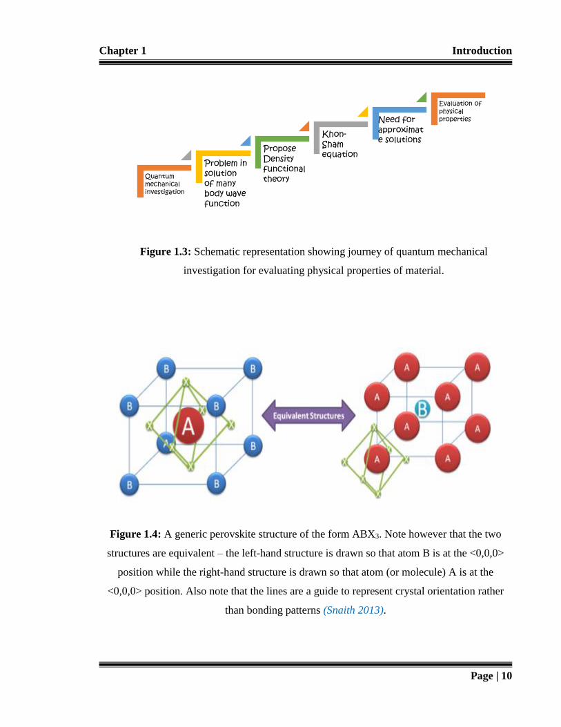
Chapter 1 Introduction
Page | 10
Figure 1.3: Schematic representation showing journey of quantum mechanical
investigation for evaluating physical properties of material.
Figure 1.4: A generic perovskite structure of the form ABX3. Note however that the two
structures are equivalent – the left-hand structure is drawn so that atom B is at the <0,0,0>
position while the right-hand structure is drawn so that atom (or molecule) A is at the
<0,0,0> position. Also note that the lines are a guide to represent crystal orientation rather
than bonding patterns (Snaith 2013).
Quantum mechanical investigation
Problem in solution of many body wave function
Propose Density functional theory
Khon-Sham equation
Need for approximate solutions
Evaluation of physical properties

Chapter 1 Introduction
Page | 11
unit cell. The larger A cation (usually a lanthanoid, alkaline earth, or alkaline earth element)
is coordinated by 12 X ions. The smaller B cation (usually a transition metal, or s/p-block
element) is positioned in the octahedral interstices formed by the X-ions (Snaith 2013 &
Navrotsky 1998).
The large flexibility of the perovskite structure makes it ideal for systematic substitutions of
the different ions in the structure. The most common substitutions are those of the A- and/or
B-site cations by other cations of different charge, size and electronic structure. The ideal
cubic perovskite structure (Pm3m) can therefore be tuned relatively easy if the difference in
the ionic radius between the ions on the same site are kept below ~10-15% (Zhang et al.,
2007). Structural changes upon substitution on the A-site, assuming rigid BO6 octahedra, can
be illustrated by the substitution of Sr2+ ions in SrTiO3 with the smaller Ca2+ ions as shown in
Figure 1.6 respectively. The example illustrates how the perovskite structure adapts changes
in the ratio between the ionic radii of the A and B cations. The resulting tilt of the BO6
octahedra is mainly the result of a minimization of electrostatic ion-ion interactions. By
treating the A and B site ions as hard spheres with different ionic radii, it is possible to
estimate the distortion of the perovskite structure from the ideal cubic Pm-3m symmetry
(Tilley 2016).
1.5.1 Tolerance factor criteria for perovskites
Tolerance factor or Goldschmidt's tolerance factor is an indicator to determine the stability
and distortion of crystal structures. Goldschmidt recognized that if the B-O distance is twice
the unit cell edge, and if twice the A-O distance equals the face diagonal of the unit cell,
perfect cubic close packing would be obtained. The relationship was quantified in the form of
(Goldschmidt 1926):

Chapter 1 Introduction
Page | 12
𝑡 =0.707<𝐴−𝑋>
<𝐵−𝑋> (1.1)
where t is now commonly known as the Goldschmidt tolerance factor. For more complex
compositions with several different A/B cations on each site, the weighted cationic radii are
used. It has been found that the perovskite structure is formed for compounds with 0.78 < t <
1.05 (Woodward 1997). The tolerance factor can therefore be used to estimate the expected
amount of octahedral tilt. For an ideal cubic perovskite, the tolerance factor should be equal
to 1. However, the cubic symmetry is also found for perovskites with t-values slightly
deviating from the ideal one. Nevertheless, larger deviations of t from 1 are followed by
changes in symmetry (Travis et al., 2016; Bhalla et al., 2000 & Mitzi 1999). The details of
some perovskites and their tolerance factors are mentioned in Table 1.1.
1.5.2 Types of perovskites
The structures of perovskites are determined by short range attractive forces and repulsive
forces between nearby ions, along with long range electrostatic interactions between unit
cells. Crystallography determines the balance of these forces, and therefore the structure.
Which, in turn, contributes to the properties and performance of the material. Depending on
composition and chemistry of the constituent elements, perovskites have five different types
like simple perovskites, inverse perovskites, double perovskites, antiperovskites, and double
antiperovskites. From the available literature it is evident that above types can be found in
five different structures, including cubic, tetragonal, orthorhombic, hexagonal, and
rhombohedral (Smith 2015). The recent advancements in identifying crystallographic
technology have made it feasible to accurately determine structure of many perovskite
compounds for subsequent modeling.

Chapter 1 Introduction
Page | 13
Figure 1.5: The ideal ABX3 perovskite structure showing the octahedral and icosahedral (12-
fold) coordination of the B and A-site cations, respectively (Navrotsky 1998).

Chapter 1 Introduction
Page | 14
Figure 1.6: Illustration of the simple cubic perovskite unit along one of the main unit cell
axes in (a) an ideal cubic perovskite with a larger A-site cation and (b) a smaller A site
cation (Zhang et al., 2007).
Table 1.1: Some perovskite, their tolerance factor and structures.
a) (Travis et al., 2016), b) (Mitzi 1999), c) (Bhalla et al., 2000)
Tolerance
factor Structure Explanation Example
>1 Hexagonal A ion too big or B
ion too small BaNiO3
a
0.93-1.02 Cubic A and B ions have
ideal size SrTiO3
b, BaTiO3a
0.71-0.9 Orthorhombic/Rhombohedral
A ions too small
to fit into B ion
interstices
GdFeO3c,
CaTiO3a
<0.71 Different structures A ions and B have
similar ionic radii FeTiO3
a
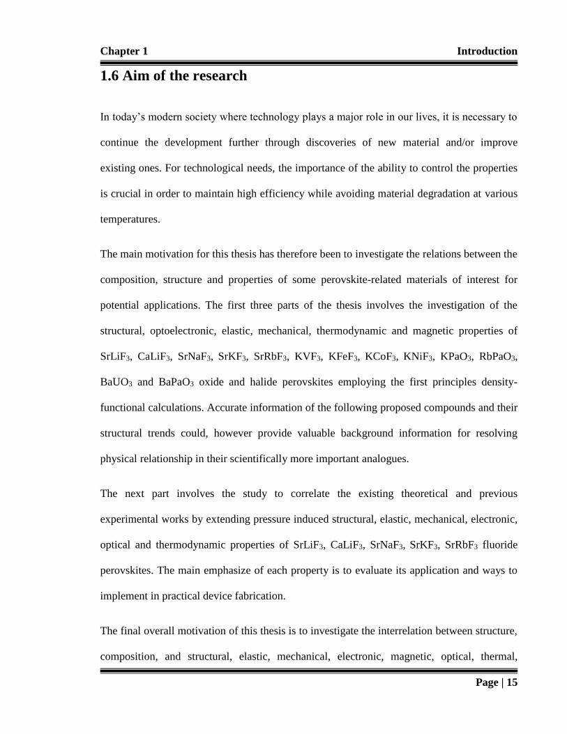
Chapter 1 Introduction
Page | 15
1.6 Aim of the research
In today’s modern society where technology plays a major role in our lives, it is necessary to
continue the development further through discoveries of new material and/or improve
existing ones. For technological needs, the importance of the ability to control the properties
is crucial in order to maintain high efficiency while avoiding material degradation at various
temperatures.
The main motivation for this thesis has therefore been to investigate the relations between the
composition, structure and properties of some perovskite-related materials of interest for
potential applications. The first three parts of the thesis involves the investigation of the
structural, optoelectronic, elastic, mechanical, thermodynamic and magnetic properties of
SrLiF3, CaLiF3, SrNaF3, SrKF3, SrRbF3, KVF3, KFeF3, KCoF3, KNiF3, KPaO3, RbPaO3,
BaUO3 and BaPaO3 oxide and halide perovskites employing the first principles density-
functional calculations. Accurate information of the following proposed compounds and their
structural trends could, however provide valuable background information for resolving
physical relationship in their scientifically more important analogues.
The next part involves the study to correlate the existing theoretical and previous
experimental works by extending pressure induced structural, elastic, mechanical, electronic,
optical and thermodynamic properties of SrLiF3, CaLiF3, SrNaF3, SrKF3, SrRbF3 fluoride
perovskites. The main emphasize of each property is to evaluate its application and ways to
implement in practical device fabrication.
The final overall motivation of this thesis is to investigate the interrelation between structure,
composition, and structural, elastic, mechanical, electronic, magnetic, optical, thermal,

Chapter 1 Introduction
Page | 16
thermodynamic properties of some selected perovskite materials for improving lens
fabrication technology, opto-electronic, spintronic and piezoelectric devices. Systematic
studies on this kind of perovskite-related materials are especially important in these strongly
correlated systems where the collective behavior of individual contributions can lead to
unexpected properties. Hopefully this study is an attempt to compensate lack of information
on theoretical and experimental data of aforementioned properties of these materials and to
add some new converged physics and innovative investigation in them. As far as, for a one-
man project, it would be too ambitious to solve all the current challenges but hopefully the
present work, does add some valuable advances in the field of ab-initio quantum mechanical
investigation.
1.7 Outline of thesis
The thesis is presented in nine chapters followed by the references. Following the
introductory chapter, chapter one, the second chapter serves to explain perovskite materials:
from synthesis to applications. The aim of Chapter 3, is to gather the general overview of
available literature on oxide and halide perovskites. Chapter 4, is reserved for the detailed
description of theory and computational details of underlying methodology, followed by brief
introduction of Density Functional Theory (DFT) and to acknowledge various simulation
techniques.
The results and discussion are discussed in four chapters (Part of the text from the published
papers is included in the respective discussion sections). Chapter 5, is devoted to investigate
elastic, and optoelectronic properties of alkali and alkaline earth fluoroperovskites
(Publication 1 to 3). Chapter 6, outlines mechanical and optoelectronic behavior of actinoid

Chapter 1 Introduction
Page | 17
based oxide perovskites (publication 4 and 5). The comparison of electronic band profiles
and magneto-optic properties of transition metal based fluoroperovskites are presented in
chapter 7 (publication 6) and chapter 8 (publication 7 to 11), distinguishes effect of pressure
variation on strontium and calcium based fluoroperovskites. The general conclusions, an
outlook and suggestions for further work are covered in chapter 9.

Chapter 2 Perovskite materials
Page | 18
Chapter 2
Perovskite materials: From synthesis to applications
“I am neither clever
nor especially gifted. I am only
very, very curious”
Albert Einstein
2.1 Overview
Perovskites obtain their name from calcium titanium oxide (CaTiO3) structure. The term
“perovskite” was initially reserved for CaTiO3, but it was later applied to synthetic
compounds with a similar stoichiometry and crystal structure to CaTiO3 (Marc and McHenry
2007). Figure 2.1 shows naturally occurring compound CaTiO3 species. Goldschmidt
(Goldschmidt 1926) extensively studied the first synthetic perovskite and pioneered many
principles that are even today, remains applicable to the structure. Recently, perovskite
structured ceramics have become one of the worldwide materials due to their peculiar
properties via ferroelectric (Choi et al., 2004), thermo-electric (Obara et al., 2004),
pyroelectric (Chan et al., 2005), dielectric (Arlt and Hennings 1985) and optical properties
(erum and Iqbal, November 2017). Depending on these peculiar properties perovskite
ceramics have several extraordinary applications such as in, random-access memories
(Kingon et al., 1996), tunable microwave devices (Nenasheva et al., 2004), capacitors
(Dimos and Mueller 1998), displays (Protesescu et al., 2015), piezoelectric devices (Uchino
et al., 1998), actuators (Muralt et al., 2009), sensors (Obayashi et al.,1976), and wireless
communications (Sebastian 2010 & Uchino et al., 1998). Perovskites can be prepared in
various forms like nanocrystalline, bulk, thin films and rods, depending on their applications.

Chapter 2 Perovskite materials
Page | 19
This chapter provides a brief overview on synthesis methods for perovskite materials,
physical characteristics, band chemistry, significant properties and at the end the chapter
highlights the eventual technological applications.
Figure 2.1: Perovskite mineral species (CaTiO3) along with Lev Aleksevich von Perovski
(Jana 2008).
2.2 Synthesis methods for perovskite materials
Historically, inorganic solid-state physics has been a very central branch of physics
industrially. Especially for the development of different technologically important materials
such as functional glasses, photocatalysts, batteries, lasers, magnetic materials, metals and
alloys, it has been and will continue to be important. The conventional “shake and bake”
solid state synthesis method (Anthony 2014) is usually enough for standard characterization
methods such as electron microscopy, although it is sometimes more beneficial to use other
routes to produce the same material, but with different morphological characteristics to

Chapter 2 Perovskite materials
Page | 20
change the size/shape dependent properties. These can be, for example, electronic and
magnetic properties in low dimensional materials or conductivity/catalytic properties from
particle size or surface mediated effects.
The following sections will briefly describe the commonly used synthesis procedures for the
unconversant reader in this field.
2.2.1 Conventional inorganic solid-state synthesis
The traditional synthesis route in inorganic solid-state chemistry has been through grinding
of the reactants, usually the oxides, carbonates or nitrates of the desired elements in
stoichiometrically right proportions in a mortar with a pestle. The corresponding mixture is
then pressed with a hydraulic press into a pellet in a dye. The pellet is then placed in a
furnace with the desired temperature programmed, in order to form the desired product (Rao
and Gopalakrishnan 1997). Due to the long diffusion lengths in the particles of the starting
materials (if oxides are used) >1μm, it is usually necessary to regrind and press a new pellet
with subsequent heating until a single-phase material is observed by powder x-ray diffraction
(Cullity 1977).
2.2.2 Solution-based synthesis methods
In some cases, it is more desirable to use a solution-based route to produce the products, for
example, when there are difficulties in obtaining single-phase materials due to unreactive
starting materials, large diffusion distances with slow diffusion rates at the desired annealing
temperature, and the need to have a high surface area and nano-sized particles of the material
for applications. Typically, the salts, e.g., nitrates, oxalates, carbonates or oxides are
dissolved in a water solution together with acid citric acid in the desired ratio to the cation
content at 70-90°C. If necessary, for example, when alkaline oxides are used, nitric acid

Chapter 2 Perovskite materials
Page | 21
needs to be used in order to dissolve the starting materials. The next step is to raise the
Potential of Hydrogen (pH) of the solution with ammonia in order to deprotonate the citrate
molecules in order to chelate - bind to the metal-ions in the solution. If any acidic oxides are
used, these will dissolve at this step.
In the next step the solution is kept at a higher temperature ~300°C to increase the solubility,
while most of the water and ammonia is boiled off. This step will also speed up the gelation
process while avoiding precipitation of any metal salts as the pH decreases when the
ammonia evaporates. The final step is to combust the citrate at a temperature above ~350°C
in order to form a nano-powder of the product. The resulting voluminous powder can then be
again grinded, pressed and annealed at higher temperatures (McHale 1995).
2.3 Prediction methods for structural properties of perovskites
To find electronic structure of any material first ingredient is its structural properties. The
electronic structure of any material is important because the properties concerned to the
electrical, magnetic, optical and thermoelectric behaviors are dependent on it (Erum and
Iqbal 2016 & Wang and Kang 1998). Structural properties of perovskites can be evaluated by
experimental as well as theoretical methods. Experimentally basic structural parameters can
be calculated by different diffraction methods such as X-ray and neutron powder diffraction
methods, powder diffraction and structure refinement methods (Cullity 1977). However
according to scope of this thesis focus is paid to theoretical methods in detail. In theoretical
fields there are several ways to determine structural properties ranging from analytical
models to computational methodology. In this lieu, the first attempt was made by Mooser and
Perason, (Mooser and Pearson 1959) they introduced structural map technology to study the
average principle quantum number by evaluating difference between anion as well as cation.

Chapter 2 Perovskite materials
Page | 22
This well-known method is called as structural map method. Kumar and their fellows
(Kumar 2008) suggested to plot “structural map” for cubic perovskites. The same method
was followed by Muller and Roy (Muller and Roy 1974).
An important feature to identify crystalline materials and their structural properties is the
lattice constant. To reduce experimental temporal cost and time, recently researchers are
aiming to develop lattice constant prediction models to accurately investigate concerned
lattice parameters. This includes seminal work based on linear regression techniques by Jiang
and their fellows (Jiang et al., 2006), Moreira and Dias (Moreira and Dias 2007), as well as
Ubic (Ubic 2007) but due to linear regression these models are incapable to attain
nonlinearity involved in correlating lattice constant with atomic parameters. As a result,
appreciably, error cannot be able to minimize. In another work Lufaso with his fellows
(Lufaso and Woodward 2001) had established mathematical model for material scientists
built on SPuDS program, that delivers structural aspects for synthesized perovskites. In 2008
another model based on number of valence electrons and average ionic radii (rav) have been
proposed by Verma and their co-fellows (Verma et al., 2008) for cubic perovskites. All these
analytical models are contributing to explore structural trends of perovskites and delivers
many useful data to academia community but there are some known limitations in these
models with comparison to computational and experimental work due to contributing factors
of equations involved in these models (Erum and Iqbal, February 2017).
In theoretical framework another way is computational methodology which includes ab-initio
or first principles investigations (Lany and Zunger 2009). In this method of calculation, the
structural parameters are predicted by volume optimization process, through reducing the

Chapter 2 Perovskite materials
Page | 23
total energy of the unit cell using Murnaghan’s equation of state (Murnaghan 1944). The
resultant ground state structural properties include various lattice parameters.
2.4 Physical characteristics of perovskites
To distinguish perovskites from other class of compounds it is necessary to have information
about its appearance and physical characteristics governing them. These compounds exhibit
variable color from gray, brown, black, and orange to yellow. On surface white to gray
streaks are observed as shown in Figure 2.2. In lustrous form it is submetallic to adamantine,
waxy or greasy. In crystalline form they are transparent and their crystals are opaque with
orthorhombic or pseudo cubic crystal symmetry. General values for hardness and specific
gravity is 5.5 and 4.0 respectively (Tilley 2016). Their associated minerals include andradite,
chlorite, leucite, melilite, serpentine, talc, nepheline, and sphene (Wenk and Bulakh 2004 &
Chakhmouradian and Mitchell 1998).
Figure 2.2: Structure and morphology of perovskite mineral (Wenk and Bulakh 2004).
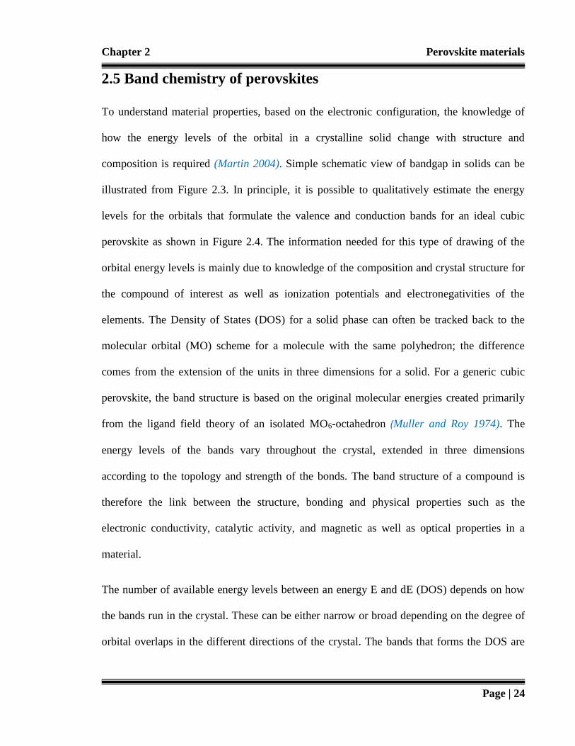
Chapter 2 Perovskite materials
Page | 24
2.5 Band chemistry of perovskites
To understand material properties, based on the electronic configuration, the knowledge of
how the energy levels of the orbital in a crystalline solid change with structure and
composition is required (Martin 2004). Simple schematic view of bandgap in solids can be
illustrated from Figure 2.3. In principle, it is possible to qualitatively estimate the energy
levels for the orbitals that formulate the valence and conduction bands for an ideal cubic
perovskite as shown in Figure 2.4. The information needed for this type of drawing of the
orbital energy levels is mainly due to knowledge of the composition and crystal structure for
the compound of interest as well as ionization potentials and electronegativities of the
elements. The Density of States (DOS) for a solid phase can often be tracked back to the
molecular orbital (MO) scheme for a molecule with the same polyhedron; the difference
comes from the extension of the units in three dimensions for a solid. For a generic cubic
perovskite, the band structure is based on the original molecular energies created primarily
from the ligand field theory of an isolated MO6-octahedron (Muller and Roy 1974). The
energy levels of the bands vary throughout the crystal, extended in three dimensions
according to the topology and strength of the bonds. The band structure of a compound is
therefore the link between the structure, bonding and physical properties such as the
electronic conductivity, catalytic activity, and magnetic as well as optical properties in a
material.
The number of available energy levels between an energy E and dE (DOS) depends on how
the bands run in the crystal. These can be either narrow or broad depending on the degree of
orbital overlaps in the different directions of the crystal. The bands that forms the DOS are

Chapter 2 Perovskite materials
Page | 25
thus affected by chemical and structural changes. In general, some simple ways to
manipulate the bands in the perovskite structure can be used and include (Hoffmann 1987):
• Isovalent or aliovalent A/B-site substitution for ions of different size and charge →
tilting of the octahedras → decrease/increase of the M-O-M orbital overlap →
narrowing/broadening of the corresponding bands.
• Substitution for more/less polarizing (electronegative) ions → more/less orbital
overlap → broader/narrower bands.
To get a more realistic picture of the energy levels of a compound it is necessary to use more
advance modeling, for example, DFT calculations (Knížek et al., 2006). Even then it is very
difficult to estimate the exact electronic structure for more complex systems. The difficulties
arise from the influences of defects, local distortions, impurities, strains, spin-orbit couplings,
mixtures of spin-states and so on.
2.6 From insulating to superconducting perovskites
Based on electronic bandgap configuration, behavior of perovskites can be classified into
insulators, semiconductors, conductors, and superconductors as shown in Figure 2.5. The
absence or abundance of free electrons play a vital role in distinguishing among the various
perovskite materials. Perovskites like SrTiO3 (Obara et al., 2004), SrLiF3, SrNaF3 (Erum and
Iqbal, March 2017), BaLiF3 (Mousa and Mamoud 2013), reveals insulating behavior. Since
they do not have any electrons in conduction band. Other perovskites like LaCuO3, KNbO3,
LaCoO3, SrRbF3, RbPbF3 (Murtaza et al., 2013 & Bringley et al., 1993) shows
semiconducting behavior. Some perovskites like LaNiO3, LaCoO3, LaMnO3, and LaCuO3
(He and Franchini 2012) manifests conductive behavior. The electrical conductivity can be

Chapter 2 Perovskite materials
Page | 26
increased by enhancing the total number of mobile charge carriers. However, the major
source of distinction between properties is electronic configuration of the B-ion. Such as do
Ti+4 is responsible for insulating character in SrTiO3, meanwhile d7 Ni3+ and d8 Cu3+ are
responsible for conductive behavior both in LaNiO3 and LaCuO3 respectively. The
corresponding d6 and d8 configuration results a splitting between the filled t2g and eg orbital
in conduction band which can give rise to insulating ground state in the corresponding
compounds.
In addition to their diverse electrical properties, perovskites have been extensively examined
for superconductivity. BaPb1-xBixO3 (0.05 < x < 0.31) discovered in 1975, is a super
conducting oxide with a critical temperature (Tc) of 13 K (Sleight et al., 1975). Since then, a
number of superconductors with Tc > 77 K including the well-known YBa2Cu3O7-δ have
been discovered (Knizhnik 2003). Now-a-days an interesting property of perovskite material
is superconductivity at high temperature. This is unique property of perovskite however the
critical temperature for superconducting transition to occur is about 130-155 K for
HgBa2Ca2Cu3O8+δ. However, the increase value of Tc is achievable by adding more number
of Cu-O layers (Chu et al., 1993). The complex compounds at a certain critical temperature
Tc includes complex cuprate perovskite oxides and their sub-units. The presence of copper
ion at B-sites is mandatory to achieve superconductivity. However, La2-xBaxCuO4 was the
first perovskite related material. Another example of such compound is BaPb1-xBixO3
(Bednorz and Muller 1986).

Chapter 2 Perovskite materials
Page | 27
Figure 2.3: Schematic illustration of the band gap in solid materials (Holgate 2009).

Chapter 2 Perovskite materials
Page | 28
Figure 2.4: A band gap diagram showing the approximate band energies in ABO3, that form
the density of states (DOS) in a perovskite (Hoffmann 1987).
Figure 2.5: A band gap diagram showing the different sizes of band gaps for conductors,
semiconductors, and insulators (Wikimedia commons 2015).

Chapter 2 Perovskite materials
Page | 29
2.7 Magnetism and electronic correlations in perovskites
When a perovskite material is put in a magnetic field, H, it gains a molar magnetization, M,
that together can be described as the magnetic induction, B, in equation (2.1) using the
centimeter-gram-system with electromagnetic units (c.g.s. e.m.u.):
𝐵 = 𝐻 + 4𝜋𝑀 (2.1)
The magnetic susceptibility can be expressed as:
𝜒𝑚 = (
𝑀
𝐻 (𝑒𝑚𝑢)).𝑀𝑊 (
𝑔𝑟𝑎𝑚
𝑚𝑜𝑙𝑒)
𝑚 (𝑔𝑟𝑎𝑚). 𝑓𝑖𝑒𝑙𝑑 (𝑂𝑒) 𝐶
𝑇 (2.2)
Here χm is the molar magnetic susceptibility in the linear response region, i.e., where the
magnetization changes linearly with the field, m is the mass in grams and Mw the formula
weight per magnetic ion. This type of linear behavior is also referred to as the Curie law,
where C is the Curie constant.
From the Curie constant it is possible to deduce the average magnetic moment per magnetic
ion through the following expression:
µ𝑒𝑓𝑓 = √3𝑘𝐵𝑇𝜒𝑚
𝑁𝐴µ𝐵2 = √8𝜒𝑚𝑇 (2.3)
where kB is Boltzmann’s constant, T the actual temperature, NA Avogadro’s constant, χm the
molar magnetic susceptibility and μB the Bohr magneton. All materials interact with a
magnetic field by responding with a force opposite to the applied field. This is called
diamagnetism and is an inherent additive property caused by the interaction of the magnetic
field with the motion of the electrons in their orbits. The effect is independent of the applied
field and temperature. The diamagnetic susceptibility is approximately in the order 10-6 emu
and negative. The opposite effect with an attractive force from the magnetization of unpaired
electrons is called paramagnetism and is several magnitudes larger, e.g., 10-4-0.1 emu and

Chapter 2 Perovskite materials
Page | 30
overrides the diamagnetic signal. The magnetic susceptibility is therefore mainly based on
two components:
𝜒𝑡𝑜𝑡 = 𝜒𝐷 + 𝜒𝑃 (2.4)
where χD and χP are the diamagnetic and paramagnetic contributions, respectively.
As a consequence of the lower thermal energy, kBT with lower temperature, an increase of
the magnetic susceptibility is observed for a paramagnetic material as more and more
electrons align in the direction of the field. The type of paramagnetism that contains some
type of cooperative orientation of the moments is better described by the Curie-Weiss law:
𝜒𝑚 = 𝑐
(𝑇−𝛳) (2.5)
Here ϴ is the Weiss constant and describes the strength of the magnetic interactions, which is
either negative (anti-parallel interactions) or positive (parallel interactions). In some cases,
the magnetic interactions between the electrons in a material can interact strongly and couple
below a critical temperature. The interactions/couplings between the magnetic centras
(unpaired electrons and orbital angular moments) are mainly classified into two major
groups, those where the majority of the electrons are coupled antiparallel (antiferromagnetic
(AFM) interactions/ordering) and those with the majority of the electrons coupled in parallel
(ferromagnetic (FM) interaction/ coupling). In between these two groups many different
types of magnetic effects/orderings can exist.
In general, the type of interactions between electrons can be described by the exchange
energy, Hex between atoms i and j separated with a distance rij with the total spins Si and Sj:
𝐻𝑒𝑥 = − ∑ 𝐽(𝑟𝑖𝑗)𝑆𝑖𝑆𝑗 (2.6)
In this expression the effective exchange parameter J(rij) describes the type of interaction
between the atoms, as a function of the distance between them. A positive value indicates

Chapter 2 Perovskite materials
Page | 31
that parallel alignment of the moments is favored and a negative value that an antiparallel
alignment is favorable. The exchange coupling can be divided into two different classes. The
direct exchange, where inter-atomic exchanges of electrons occur through atoms that are
close enough for their orbitals to overlap significantly, and indirect exchange, which couples
the magnetic moments over larger distances through intermediate ions such as oxygen ions in
oxides. The latter is commonly referred to as super-exchange. It follows that a material in
which the magnetic moments are spontaneously aligned in the field direction below a defined
temperature, i.e., the Curie temperature, TC, is a FM. In this type of material, the
magnetization increases rapidly and saturates quickly with M as the larger magnetic domains
grows at the expense of the smaller.
As opposed to FMs with one magnetic cell, the magnetic moments of two identical sub-
lattices can align oppositely with identical magnetic moments below a certain temperature,
i.e., the Neel temperature, TN. The material is referred to as an AFM. Hence, it is not possible
to have an AFM ordering in non-crystalline solids. A special case of AFM ordering called
ferrimagnetism occur when the two sublattices are chemically different although
ferromagnetically ordered in each sub-lattice, that results in a residual net magnetic moment.
Hence, ferrimagnetic ordering can exist in amorphous materials as the oppositely aligned
magnetic moments are not required to be of the exact same size.
Due to local variations in a material that cause anisotropical variations in the crystal field
strength, meta-magnetism can occur, which is typically an AFM below the TN but undergoes
a magnetic transition at high field strengths that causes the magnetization to increase. This
can be observed as a change in the slope in the M vs. H curve at fields exceeding the
saturation of the magnetization.

Chapter 2 Perovskite materials
Page | 32
Another type of magnetic behavior of solids is the so-called speromagnetism, which involves
randomly ordered localized magnetic moments with no significant net magnetization or
ordering beyond the nearest neighbors, except for randomly coupled spins locally. These
systems are usually referred to as spin glasses and behave mainly as a paramagnet above the
“freezing” temperature TSG.
Above a certain concentration of magnetic ions, clustering can occur, where the material is
classified as a mictomagnet which essentially is a “cluster glass” (Mattis 2006). Spin glass
behavior can be characterized by using A.C. magnetic measurement instead of D.C. that only
measures the equilibrium value of the magnetization. The A.C. susceptibility measures the
susceptibility as a function of the variation of the field, H and frequency ω that varies
sinusoidally. This will provide a high sensitivity to the change of magnetization at a given
time and frequency. For spin glasses the freezing temperature will show a shift in the
temperature of the “cusp” with changing frequency of the field due to relaxations and
irreversible ordering at non-equilibrium conditions (Stein and Newman 2012).
In transition metal compounds the measured effective magnetic moment, ueff can often
deviate significantly from the calculated value given by the expression (Handley 2000):
µ = [𝐿(𝐿 + 1) + 4𝑆(𝑆 + 1)]1
2 µ𝐵 (2.7)
where L is the maximum value of the orbital quantum number, S the total spin quantum
number, for the electrons outside closed shells and µB bohr magneton. The total angular
momentum J = |L + S| is conserved and the degeneracy of the energy levels for a specific J
value will be either (2S + 1) or (2L + 1), depending on which one has the smallest value.
With a “spin-orbit” coupling new quantum states are created for each J with a degeneracy of
2J + 1. Adjacent energy levels, e.g., J and J + 1 will then be separated by an energy

Chapter 2 Perovskite materials
Page | 33
corresponding to (J + 1) λ, for which λ is the spin-orbit coupling constant with the unit of cm-
1. For strong spin orbit couplings, the energy separation will be relatively large and can thus
be seen clearly by spectroscopic methods, e.g., XANES.
For many of the 3d transition metal compounds, the observed magnetic moment frequently
deviates from the values that includes spin-orbit coupling, and are therefore closer to the
spin-only value of the effective magnetic moment:
µ𝑆.𝑂 = [4𝑆(𝑆 + 1)]1
2 = [𝑛(𝑛 + 2)]
1
2 µ𝐵 (2.8)
where n is the number of unpaired electrons responsible for the magnetic moment. In these
cases, the orbital angular momentum is either very small or negligible; hence the orbital
contribution is “quenched” (Mabbs and Machin 2008).
2.8 Thermodynamic valence stability in transition metal based
perovskites
The properties of the perovskites primarily depend on the electronic structure of the
constituting ions and their interactions through bonds. However, properties such as the
electronic or ionic conductivity can deliberately be changed by taking advantage of the
thermodynamic stability of different transition metal ions in their different oxidation states.
In general, the thermodynamic driving force for a reaction is to minimize the Gibbs free
energy, ΔrG towards zero to reach equilibrium. For a spontaneous reaction the ΔrG is lower
than zero, that is, ΔrG < 0 and ΔrG > 0 for a non-spontaneous reaction via following
equation:
𝛥𝑟𝐺 = 𝛥𝑟𝐻 − 𝑇𝛥𝑟𝑆 (2.9)
Here ΔrG is the Gibbs free energy of reaction, ΔrH the enthalpy of reaction, ΔrS the entropy
change of reaction and T the actual temperature. It is clear that metals with a large negative

Chapter 2 Perovskite materials
Page | 34
ΔrG for the reaction with oxygen to form an oxide; also form the oxide much more easily.
Hence, oxides with the least negative ΔrG, are reduced more easily. In general, the trend
among the 3d transition-metal elements can roughly be approximated to the following order,
where the oxide form of the first element is the easiest to reduce to metal at 1000°C: Ni > Co
> Fe > Mn > V > Cr > Ti (Kawada and Yokokawa 1997). However, although this trend is
true for the binary BxOy-oxides, it is important to emphasize that the same trend is also
observed for the corresponding ABO3 perovskites.
As an additional difference between the perovskite oxides and the simple binary oxides, the
higher valence for transition metal ions of varying oxidation states in perovskites are further
stabilized through the lanthanide ion; therefore, an additional term called the stabilization
energy δ(ABO3) needs to be reduced. However, it is observed that the stabilization of higher
oxidation states in the LaMO3 decreases with a decrease in the Goldschmidt tolerance factor,
t (Goldschmidt 1926). This implies that a higher oxidation state of the transition metal ion is
better stabilized for structures with high symmetry.
2.9 Properties of perovskites
A property is an attribute which describes the features of any system. The properties can be
classified in terms of physical and/or chemical as shown in Figure 2.6. A physical property is
an aspect of matter that can be measurable without changing it and whose value describes
state of the physical system. Some examples of physical properties are molecular weight,
volume and color. Chemical properties are contrasted with physical properties which use to
determine the way a material behaves in a chemical reaction and it can only be observed by
changing the chemical identity of a substance. According to the need of this thesis attention
is only paid to physical properties of perovskites.

Chapter 2 Perovskite materials
Page | 35
Many examples of perovskite compositions with various interesting properties can be found
in the literature. For example, some compounds exhibiting colossal magnetoresistance
(CMR) are the perovskite related La1-xAxMnO3+δ materials where A2+ is Ca, Sr, Ba, or Pb
(Van et al., 1993). Compounds exhibiting CMR have potential uses in data storage
technologies, such as computer hard drives and floppy disks. Different perovskite
compositions also result in a wide variety of electrical behaviors. For example, SrFeO3 is a
metallic conductor at room temperature, BaBiO3 is a semiconductor and stoichiometric
LaMnO3 is an insulator (Muller and Roy 1974). Due to these tunable properties of perovskite
materials, very large variety of applications can be obtained and many more are still to be
found in the future.
Figure 2.6: Block diagram breakdown of chemical and physical properties of matter.

Chapter 2 Perovskite materials
Page | 36
2.9.1 Property based tentative classification of perovskites
Perovskite materials possess various versatile properties. Based on these properties one can
tentatively classify perovskites into the following major groups such as semiconducting,
conducting, and superconducting perovskites, dielectric perovskites, piezoelectric
perovskites, pyroelectric perovskites, ferroelectric perovskites, ferro-magnetic and anti-
ferromagnetic perovskites, colossal magnetoresistive perovskites, photovoltaic perovskites,
and catalytically active perovskites. Based on these properties perovskite materials can
classify accordingly.
2.9.2 Opto-electronic properties
Perovskites have emerged as a revolutionary class of materials having excellent optical and
photoluminescence properties. Several areas where the light interacts with the matter are
obviously of practical interest. Studies of the optical properties of solids have been proven as
a strong tool for electronic and atomic structure of the desired materials. The optoelectronic
properties of a material are important to understand the optical nature over a wide spectral
range to acknowledge the application of that material in photonics and optoelectronic
devices. The major requirements for these devices are wide and direct bandgap
semiconductors (Fox 2001). It helps to identify the internal character of that material
(Wooten 1972). Perovskites have gained huge hype in opto-electronic industry due to direct
wide bandgaps and high thermal stability. SrThO3, SrZrO3, and SrRbF3 have direct wide
bandgap semiconductors, (Shein et al., 2007) which makes these oxide and halide
perovskites very favorable for usage in optoelectronic applications. The optical density of
CaTiO3 was reported by Linz and Herrington (Linz and Herrington 1958). The absorption

Chapter 2 Perovskite materials
Page | 37
characteristics are quite similar to those of SrTiO3 crystals with the exception that the
absorptions are shifted to shorter wavelengths. BaTiO3 and SrTiO3 have been considered for
high temperature infrared windows. The electro-optic properties of KTaO3, K(Ta0.65Nb0.35)
O3, BaTiO3 and SrTiO3 in the paraelectric phase were measured by Geusic and their fellows
(Geusic et al., 1964). The electro-optic coefficients of these perovskites are nearly constant
with temperature and can vary from material to material when the distortions of the optical
indicators are expressed in terms of the induced polarization. Many ab-initio or first
principles investigation have successfully explored the opto-electronic properties of these
materials which are in reasonable agreement with the experimental studies.
Now-a-days, there has been considerable attention in resources to be used for laser
applications. Using of perovskite laser host materials is a great deal. The ion Nd3+ appears to
be the most popular for introduction into relatively large crystallographic sites. However,
except when LaF3 is used as a host, compensating ions are required in these substitutions.
Divalent Tm2+ and Dy2+ can be substituted in CaF2 without compensating ions but these
divalent rare earth ions relatively unstable. For crystallographic sites for the Al3+, Cr3+ proved
to be ideal for substitution.
In photovoltaic industry, originally the perovskites were viewed as a curious replacement to
dye molecules in mesoscopic type of sensitized solar cells, due to their high absorption
coefficient and broad sense of absorption spectrum. However, it was soon realized that
perovskite materials are unique semiconductors, different from dye molecules or other
organic absorbers, and very suitable for the inorganic semiconductors for photovoltaic
applications, for example Si or GaAs. The perovskites materials have long carrier diffusion
length and remarkable performance in planar heterojunction architectures. The conversion

Chapter 2 Perovskite materials
Page | 38
efficiency of perovskite solar cells has reached up to 16% in its current version. The fast-
paced improvement, coupled with inexpensive materials and preparation methods indicates
that perovskite solar cells can break the prevailing paradigm and can be achieved in low cost
and excellent performance. In addition, multi-junction hybrid solar cells based on perovskites
are a very promising route to deliver a higher efficiency, cost-effective solar technology that
will compete favorably with today’s technologies, and we believe this application is likely to
be the first commercial appearance of the perovskite solar cells. Due to hysteresis free, such
cells inherit the advantages of organic photovoltaics. These benefits will lead these
perovskites go beyond the crystalline silicon (Chen et al., 2015).
Bandgap tailoring is another technique to design new materials for application in
optoelectronic industry. There are many theoretical and experimental techniques to vary
bandgap of materials to make them applicable for optoelectronic applications. The perovskite
photovoltaics can be processed on a variety of substrates via either solution or vapor phase
processing and have already delivered very high efficiency on a flexible format. In particular
fun illustration of the future technologies may enable extremely lightweight high-power
perovskite photovoltaics (Holgate 2009).
2.9.3 Dielectric properties
The detailed study on dielectric properties of perovskites have been done in the recent past
because some perovskites have revealed interesting unusual high value of the dielectric
constant, in which BaTiO3, PbTiO3 (Chou and Chen 1998), BaUO3, BaPaO3 (Erum and
Iqbal, February 2017), are worthy to mention. This feature of any compound is highly
desirable in micro as well as nano electronic devices, especially in their capacitive and
thermistive components. In oxide perovskites, such as PbTiO3, BaTiO3, and BaUO3 the

Chapter 2 Perovskite materials
Page | 39
collective polar displacement of metal ion on B site of perovskite, in accordance with oxygen
sub-lattice is responsible for large value of dielectric constant which can be associated with
their ferroelectric behavior (Charmola et al., 2011). The complex form of perovskite solid
solution attains a growing interest in last few decades because of numerous unexpected
properties. Relaxer ferroelectric is a class of perovskite compounds which retains pronounced
frequency dispersion and large value of dielectric constant and variation in the value of
dielectric constant as a function of temperature, which is of potential interest in
manufacturing practical devices. It is a well-known fact that dielectric property, response to
external excitations. The solid solutions of these ferroelectric materials are disordered by
variation in doping concentration and their dielectric behavior can be controlled by
controlling concentration of doping in them. This concerns several groups of materials
termed as mixed metal perovskites “super Q” solid solution such as SrxCa1-xTiO3, BaxSr1-
xTiO3, PbZn1/3Nb2/3O3-xPbTiO3, PbMg1/3Nb2/3O3-xPbTiO3 (Wu and Davies 2006). There are
many other useful techniques to control dielectric response of perovskites such as application
of pressure, temperature and so on. These properties widen the significance of these
materials while provoking future efforts to study such material under different conditions.
According to the value of dielectric constant and associated parameters perovskite
compounds exhibit many intriguing applications. Among them an important application is in
metal-oxide semiconductor field effect transistor (MOSFET). The perovskite oxide
CaCu3Ti4O12 is known to display largest value of dielectric constant between 104-105
(Alonso et al., 2003 & Sinclair et al., 2002). This class of compound is classified as giant
dielectric constant materials (GDM). The reason behind this value is still under investigation
however one possible reason is reported, regarding to barrier layer capacitor model. The

Chapter 2 Perovskite materials
Page | 40
major utilization of dielectric constant lies in the fact that it can eventually determines the
miniaturization capacity of electronic component. Now-a-days material scientist are
struggling hard to explore the ties between structural and dielectric properties, in order to
utilize them in future applications and each of above mentioned factors needs to be a subject
of special investigation (Homes 2001).
2.9.4 Piezoelectricity
The root of piezoelectric properties lies in between two crucial words piezo and electrics.
Hence the combined meaning of the word implied the concept of pressure-electricity. The
materials which retains this phenomenon conversely possesses geometric strain or
deformation in proportion to an applied electric field as shown in Figure 2.7. The
piezoelectric effect was first discovered in 1880 by curie brothers in single crystal quartz
(Katzir 2003). The perovskite material which can well be known as the dawn of piezoelectric
material is the ceramics of Barium titanate (BaTiO3). However original discovery of BaTiO3
was not concerned with piezoelectric properties rather it was related to high capacitance
(Ogawa 1947). Now-a-days the widely commercialized perovskite ceramics are primary
piezoelectric materials (Jaffe and Cook 1971). These piezoelectric type of perovskite
materials are applied to various devices ranging from sensors to actuators. There are five
essential key ingredients in the development of piezo-materials which includes performance
to reliability, macro to nano, hard to soft, homo to hetero, and single to multi-functional.
There are many perovskites including simple to complex one which exhibits piezoelectric
property. For example Ba (Mg1/3Ta2/3)O3, Pb(Mg1/2W1/2)O3, and Ba(Mg1/3Ta2/3)O3. Other
examples of lead free piezoelectric includes three major group of compounds namely (Bi,
Na)TiO3, (Na,K)NbO3, and tungsten bronze based perovskites (Uchino 2014). From

Chapter 2 Perovskite materials
Page | 41
crystallographic point of view depending on B-ion ordered/disordered arrangement some of
these structures show simple/complex perovskite symmetry. The significant difference in
physical properties of these compounds is observed corresponding to ionic ordering because
on increasing the ionic valence difference, tendency of short-range ordering increases. High
K-piezoelectric perovskite are applied to study medical acoustic. Another astonishing
application of piezoelectric Pb(Zr,Ti)O3 perovskite is its ability of passive mechanical
damping. Furthermore, it can also be utilized in piezoelectric microelectromechanical system
(MEMS) (Roberts 1947). However, from technological point of view some emphasize is
required to utilize piezoelectric property of perovskite in new technologies such as ultrasonic
disposal technology, in reduction of gas contamination, in generating new energy-harvesting
systems and in developing economic medical instruments. In disaster prevention application
piezoelectric perovskite can play a vital role. These applications include nuclear power plant
safety systems, earthquake monitoring as well. In actuator materials the primary (linear) and
secondary (quadratic) phenomenon are piezoelectric and electrostatic effects respectively.
Certain perovskite oxides, for example solid solutions of PbZrO3 and PbTiO3, exhibit
piezoelectric properties and are used for numerous applications including microphones,
stereo speaker fuses (for lighters) and ultrasonic cleaners (Jaffe and Cook 1971).

Chapter 2 Perovskite materials
Page | 42
Figure 2.7: Schematic illustration for the phenomenon of piezoelectric effect (Uchino 2010).
2.9.5 Multiferroicity
“Materials should exist, which can be polarized by a magnetic field and magnetized via
an electric field.” (Curie 1894)
Multiferroics symbolize an extraordinary class of materials exhibiting simultaneous
ferromagnetic, ferroelectric and ferroelastic ordering. Figure 2.8-2.10 depicts the multiferroic
materials possessing respective properties. The distinctiveness of these materials lies on the
possibility of simultaneous utilization of both their magnetization and polarization states, a
massive potential which would make them outstanding candidates for new generation
memory devices and sensors (Scott 2007 & Ramesh and Spaldin 2007).
Multiferroic perovskites can be classified into different groups which exhibits in two coupled
ferroic order (vice-versa antiferroic order) distinguishing between two major classes of
multiferroic materials. These two groups are responsible for two major properties, namely
ferroelectricity and ferromagnetism. Some special perovskites retain both ferroelectric and

Chapter 2 Perovskite materials
Page | 43
ferromagnetic behavior at the same time such as BiFeO3, BiCrO3, and BiMnO3, are the
materials which shows multiferroicity even at room temperature (Bordet et al., 2007).
Figure 2.8 depicts perovskite materials with regard to their ferroelectric, ferromagnetic and
multiferroic character. Among the various explored multiferroics, BiFeO3 oxide perovskite,
is receiving nonstop attentions since it possesses both ferroelectric order and anti-
ferromagnetic order for a widespread temperature range which is greatly above room
temperature (Ederer and Spaldin 2005). Another example includes BiMnO3 contain Mn ion
which is associated with mixed perovskite state with d0 and dn ions simultaneously in
dissimilar ionic states. The origin of multiferroic compound starts from the discovery of first
ferromagnetic material which was complex combination of several multiferroic boracite
compounds known as nickel iodine boracite Ni3B7O13I (Ascher et al., 1966). The coupling
factor is very weak and rare in these perovskites.
There are several sources of ferromagnetism and ferroelectricity in multiferroic materials.
However, these two phenomena try to exclude one another. Multiferroic materials are single
phase materials which is combination of two or more forms of ferroic order including
ferromagnetism, ferroelectricity, ferroelasticity, and ferrotoroidicty (Scott 2007). Block
diagram illustration of perovskite multiferroics are presented in Figure 2.9. However, these
materials are rare in nature because the d-transition metal ion (which is essential for
magnetism), generally reduces the capacity of off-centering ferroelectric distortion. In order
to simultaneous co-existence of ferroelectricity and ferromagnetism an additional driving
force must be present. Some multiferroic materials have strong response towards both
electric and magnetic field at room temperature that is why very rare of them are used in

Chapter 2 Perovskite materials
Page | 44
practical applications. A ferroelectric material must be an insulator and most of the
ferromagnetic materials are generally metals (Ascher et al., 1966).
“You may say anything you like but, we all are made up of ferroelectrics”
(Matthias 1949)
Hence, the absence of ferromagnetic insulators limits the concurrent manifestation of
ferromagnetic and ferroelectric ordering. Figure 2.10 reveals crossed interaction between
ferroelectricity and ferromagnetism. However schematic illustration of both phenomenon is
presented in Figure 2.11. Magnetic ordering of any kind takes place due to the presence of
unpaired d electrons, whereas ferroelectric materials such as common perovskite oxides
(ABO3) have a d0 configuration on the small B cation. Magnetoelectric multiferroic materials
should have some distortion in the crystal structure with some unpaired electrons in the d
orbitals. Recently, it has been found that even in the absence of any structural distortion,
magnetic spin ordering can produce ferroelectricity. This greatly expands the number of
potential ferroic materials (Cora and Catlow 1999).
Now-a-days modern research is focused on the materials which have the ability to bear
ferroelectricity with ferro or anti-ferro magnetic state simultaneously. This type of modern
multi multiferroic materials have potential applications in hybrid memory and spintronic
devices because of advantage of no time reversal and spatial symmetry. Advantages of these
multiferroic materials includes highly sensitive magneto-sensors, multistate memory
elements, and sensitive detection of magnetic field. However, there are some challenges that
BiFeO3 type of multiferroic materials have to face such as the value of leakage current is
very large in them, retaining small remnant polarization with commonly high value of
coercive field. However, the current challenges with BiFeO3 type of perovskite compounds

Chapter 2 Perovskite materials
Page | 45
can be overcome by applying electric field by introduction of manganese and titanium in
BiFeO3, in order to reduce the amount of leakage current greatly.
2.9.6 Electronic conductivity
Electronic conduction in perovskite-related materials is one of the main properties that
governs the feasibility of the material for many applications, for example, catalysts (Li et al.,
2009), thermoelectrics (Kobayashi et al., 2001), spintronic devices (Serrate et al., 2007) and
in various electrodes (Molenda et al., 2007) as well. In 3d, 4d or 5d transition metal-based
perovskites, different types of bonding to the oxygens should be expected. In general, the
nuclear charge is more efficiently screened by the closed shells when moving down in the
periodic table. It is therefore expected that the outer electrons are more loosely bonded for 5d
elements relative to 3d elements. Therefore, the hybridization of the d-orbitals with the
oxygen 2p orbitals should be larger for 5d-elements. The orbital overlap of the metal-oxygen
(M-O) or metal-halide (M-H) bond governs a large part of the localization of the electrons.
Using a band picture this can be described with the large overlap of the M-O/M-H orbitals
that lead to broader bands, and hence higher electronic conductivity. The behavior of the
electrons can be generalized into two types, itinerant and localized. The itinerant picture
approximates the electron as a “cloud” and hence electrons that travel through the material
without any major resistance. This type of behavior is typical for metallic oxides such as
CaVO3, SrCoO3 and SrMoO3 (Goodenough 1967). For the localized picture, it is assumed
that the orbital overlap is not large enough for the electrons to move freely, i.e., the inter-
atomic distances are larger than the itinerant electron case. This results in particle-like
electrons “jumping” from one cation to another, and hence the conductivity will be activated

Chapter 2 Perovskite materials
Page | 46
Figure 2.8: Multiferroics combine the properties of ferroelectrics and ferromagnets.
Figure 2.9: Block diagram illustration of perovskites multiferroics

Chapter 2 Perovskite materials
Page | 47
Figure 2.10: The multiferroics totem; illustrating the three main ferroic orders with their
respective fields and crossed interactions (Wang et al., 2015).
Figure 2.11: Conditions required for ferroelectricity (polarization) and ferromagnetism
(unpaired electron spin motion) (Mabbs and Machin 2008)

Chapter 2 Perovskite materials
Page | 48
by thermal energy, which increases the probability for a successful “jump” as the thermal
vibrations increases. These types of materials behave as semiconductors for which the
conductivity increases with increasing temperature. In fact, conductivity does not give any
information about the majority type of carrier, i.e., electrons/holes and will therefore need to
be complemented by measurements of the Seebeck coefficient.
2.9.7 The Seebeck coefficient
When a part of material is exposed to heat, charge carriers, i.e., electrons and holes will start
to diffuse to the cold part. The accumulation of one type of charge carriers at the colder part
will give a difference in chemical potential that corresponds to an electric potential difference
ΔV, i.e., the Seebeck voltage. The created potential difference will depend on the material’s
ability to separate the two different “heat carriers,” mainly the negative electrons, e, and the
positive holes, h. Hence, the build-up of the Seebeck voltage will depend on the mobility of
the two types of carriers and will thus be different from one material to another. This effect
arises from the entropy change induced per charge carrier, e.g., spin, mixing and vibrational
contributions. The calculation of the Seebeck coefficient can be defined in different ways
depending on type of material (Kobayashi et al., 2001).
2.9.8 Polarons
Many of the perovskite materials exhibits the phenomenon of lattice vibrations. When the
lattice phonons (lattice vibrations) are small enough (appropriate wavelength) to match the
local deformations caused by the electron when moving through the lattice, a potential well is
formed. The electron is therefore trapped by the lattice deformation caused by the local
dielectric polarization of the lattice. The electron and its lattice distortion behave as one unit,
Chapter 2 Perovskite materials
Page | 49
which is most often classified as a polaron. When the wave function and the corresponding
lattice distortions cover many lattice sites, a so-called large polaron is formed. The large
polaron moves as a free electron through the lattice and is not entirely trapped, hence the
metallic behavior of transition metal oxides when electronic conduction is dominated by
large polarons (Cox 1992). In cases where the interaction of the electron with the lattice is
large enough, i.e., polaron-binding energy is larger than half the band width of the electron,
the electron will be classified as a small polaron (Goodenough 1971). The conduction
through small polaron-hopping is thermally activated and will often lead to a semi-
conductive behavior of the transition metal oxide and fluorides.
2.9.9 Thermal expansion
All perovskite materials are vibrating at all temperatures, even at absolute zero the atoms still
vibrate inside a material. As the temperature increases, the thermal energy of the system
increases, which in turn gives the atoms more kinetic energy to increase their vibrating
motion anharmonically and thus occupy a larger volume. The thermal energy not only
increases the volume of the atoms but can also induce more drastic changes in the atomic
volume in the crystal. This includes the reduction of the transition metal ion through the
formation of anion or cation vacancies or changes in the electronic structure from thermal
excitation of one spin-state to a higher spin-state as in Co3+ (Shannon 1976). In other cases,
the thermal energy will at some point induce a phase transition that can be either a change in
the state, e.g., solid to liquid to gas phase or a structural change within the same, e.g., solid to
solid state. If such transition occurs, it will, if the change in the unit cell volume is large
enough, be seen in the thermal expansion of the material. For solids, it is common to measure

Chapter 2 Perovskite materials
Page | 50
the average linear expansion of a pressed and sintered powder along one direction by a
dilatometer. Typically, the sintered cylindrical pellet that is to be measured is polished to a
size close to the sapphire reference used for calibrating the instrument. The linear thermal
expansion is measured as a function of temperature in one dimension and can be roughly
calculated over a temperature range.
2.10 Application of perovskites
Perovskite materials exhibit intriguing and extraordinary physical properties that have been
extensively studied for both theoretical modeling and practical applications. These solids are
currently gaining considerable importance in the field of electronics, geophysics,
astrophysics, nuclear, optics, medical, and environment as well (Housecroft and Sharpe
2008). Oxide and halide based perovskites are fascinating nanomaterials for wide
applications due to its structural stability, wide bandgaps, variety of available compounds,
large number of intriguing properties, that eventually lead to many real-world applications.
The ABX3 type halides and oxides with direct band gaps (> 3 eV) have strong stability
against high temperature and strong radiation. Thus, the wide band gap ABX3 type halides
and oxides are potential candidates for next generation UV photodetectors, vacuum
ultraviolet transparent lens martials, vacuum-ultraviolet light emitting Diodes (VUVLEDs)
(Erum and Iqbal, March 2017 & Roth 1961). These materials demonstrate diversified
physical phenomenon such as piezoelectric, pyroelectric, ferroelectric, dielectric,
superconductive, multiferroic, Colossal Magnetoresistance (CMR), and Giant
Magnetoresistance (GMR) etc.
The strontium and barium based perovskites (BaZrO3 and SrZrO3) are currently being
developed as the electrolyte material for Solid Oxide Fuel Cells (SOFCs) (Gemmen and Liu

Chapter 2 Perovskite materials
Page | 51
2010). Perovskites have an unusually high tolerance for oxygen ion vacancies, which makes
it an ideal electrolyte or cathode material for fuel cells. Oxygen vacancies can be created in
the material by doping with rare earth elements such as Y(III) or Yb(III), which replace the B
atom, and create one oxygen vacancy in order to maintain charge neutrality. These randomly
distributed oxygen vacancies can significantly change the conductivity of the material and
make it a very efficient electrolyte (Winter and Brodd 2004). Another current area of
research involving perovskites is high-temperature superconductors (HTSCs). The cuprate-
perovskite type is a specific kind of superconducting material. Cuprate perovskites are
related to CaTiO3 type perovskites but differ in that the B atoms have eight-fold coordination
with oxygen atoms. Starting from the CaTiO3 prototype and going to YBa2Cu3O7, Ba and Y
substitute for Ca, while Cu substitutes for Ti (Smith et al., 2011). Some cuprate-perovskite
ceramic HTSCs currently have an operating temperature of 90 K, which is significantly
higher than most other superconducting materials. Furthermore, various applications of
perovskites such as solar cells, Light Emitting Diodes (LED), Photodetectors, waveguides
and nano lasers at different length scales can be illustrated from Figure 2.12. Table 2.1 gives
some more important applications of different perovskite structured materials along with the
respective properties.
Depending on these distinct properties perovskites are useful for numerous applications for
example (Das 2017; Alvarez 2016; Dogan 2015; Brittman 2015; Benedek and Fennie 2013;
Raveau 2005 & Shaw 2000):
• Thin film capacitors
• Non-volatile memories
• Photo electrochemical cells

Chapter 2 Perovskite materials
Page | 52
• Recording applications
• Read heads in hard disks,
• Spintronics devices
• Laser applications
• For windows to protect from high temperature infrared radiations.
• High temperature heating applications (Thermal barrier coatings)
• Frequency filters for wireless communications
• Non-volatile memories
• Sensors, actuators and transducers,
• Drug delivery
• Catalysts in modern chemical industry
• Ultra-sonic imaging, ultrasonics & underwater devices

Chapter 2 Perovskite materials
Page | 53
Figure 2.12: Various applications of perovskites quantum dot, nanowire and nanosheet
(Wang and Kang 1998).

Chapter 2 Perovskite materials
Page | 54
Table 2.1: Applications of perovskites along with respective properties (Das 2017; Alvarez
2016; Dogan 2015; Brittman 2015; Benedek and Fennie 2013; Raveau 2005 & Shaw 2000)
Reference
compound
Properties Possible/ Actual
applications BaTiO3 Dielectric
Ferroelectric
Multilayer ceramic capacitors
(MLCCs),
sensor, PTCR resistors,
embedded capacitance
PbTiO3 Pyroelectric
piezoelectric
Transducer, pyrodetector, under
water devices
(BaSr)TiO3 Non-linear dielectric
properties,
pyroelectric
Tunable microwave devices,
pyrodetector
Pb(ZrTi)O3 Dielectric,
Pyroelectric,
Piezoelectric,
Electro-optic
Nonvolatile memory,
ferroelectric memories,
Surface wave acoustic devices,
pyrodetector,
substrate wave guide devices
Bi4Ti3O12,
high Tc cuprate
compounds
Ferroelectric with high
Curie temperature
superconductivity
High-temperature actuators,
FeRAMs
BaCeO3, BaZrO3 Proton conduction Electrolyte in protonic solid
oxide fuel cells (PSOFCs)
LaNiO3 chemical catalysts
(La,Sr)MnO3 Colossal Magnetoresistance Spintronics devices
Pb(Mg1/3Nb2/3) O3,
CaCu3Ti4O12,
Pg3MgNb2O9
dielectric Memory, capacitor
Resonators,
K(TaMb)O3 Pyroelectric,
Electro-optic
Waveguide device, frequency
doubler
BiFeO3 Magnetoelectric coupling,
high Curie temperature
Magnetic field detectors,
memories
(La,Sr)BO3
(B = Mn, Fe, Co)
Mixed conduction, catalyst Cathode material, oxygen
separation
membranes, membrane
reactors, controlled
oxidation of hydrocarbons
BaTiO3,
(K0.5Na0.5) NbO3,
Na0.5Bi0.5TiO3
Ferroelectricity,
piezoelectricity
Computer Memory, Lead-free
piezoceramics, Ultrasounds
SeCuO3 multiferroicity Memory Devices
LaAlO3
YAlO3
Host materials for rare-earth
luminescent ions
Lasers Substrates for epitaxial
film deposition
SrTiO3, SrLiF3 Insulators Microelectronics
Ba2MgTa2O9 Highest Melting Point Space Craft

Chapter 3 Literature Review
Page | 55
Chapter 3
Literature Review
“If you have an apple and I have an apple and we exchange apples
then you and I still have one apple.
but if you have an idea and I have an idea and
we exchange ideas,
then each of us will have two ideas”
George Bernard Shaw
3.1 Overview
To understand science, it is necessary to know its history. This section of the work is
contextual area of the research to justify and ensure existing body of knowledge and
illustrates the vision that, in which extent subject has been studied previously while
highlighting the flaws and gaps in the previously studied work. Further it enhances concern
of the work, add understanding and knowledge in the field of study, establish a theoretical
framework between methodology and the material. In this chapter, the previous research
work carried out on oxide and halide perovskites are reviewed briefly. In general, this chapter
provides background on physical properties of perovskites with broad-line of interest.
3.2 Background of materials
In perovskites, metallic and non-metallic elements are combined together to form an ideal
cubic solid structure. They equip properties of ceramic materials and are abundantly found in
earth’s crust. The perovskites are composed of calcium titanium oxide mineral which is
based upon calcium titanate. It contains the chemical formula ABX3 having three

Chapter 3 Literature Review
Page | 56
compositional variables A, B, and X. Here A is usually large cation like Rb, Na, K, Ca, Sr,
and Ba; B is supposed to be smaller cation like Ti, Nb, Mn, Co, Fe, and Zr; and X anion can
be halides, hydrides and oxides such as F, Cl, I, Br, H, O) (Brik 2011). (The detailed
description of perovskite and its structure can be found in Chapter 1 and 2).
Configuration of different ions in perovskite family of compound provide information about
its basic structure however perovskite structure can be deviated from idealized crystal
structure due to several reasons so knowledge about different properties of idealized & non-
idealized compounds are extremely important. The rapid improvement in physical properties
such as structural properties, mechanical properties, opto-electronic properties, magnetic,
electromagnetic and magneto-opto-electronic properties, thermal, thermoplastic,
thermoelectric, thermomechanical, and thermodynamic properties, vibrational and dynamical
properties of perovskites has gained huge interest from academic community. In fact, they
are rising star of the exploration world. These exceptional physical properties exhibit many
exotic applications, revealing many intriguing features like:
Ferroelectricity as in BiFeO3 (Arnold et al., 2009), Paraelectricity as in SrTiO3 (Salehi 2011).
Thermoelectricity as in LaCoO3 (Anzai et al., 2011 & Androulakis et al., 2004), in
CH3NH3AI3 (A = Pb and Sn) (He et al., 2014), in Ni-doped perovskite-type YCo1-xNixO3 (Yi
et al., 2013), in HoMnO3 (Khan et al., 2015), in SrTiO3 (Muta et al., 2004 & Ohta et al.,
2005) and in CaMnO3 (Kobayashi et al., 1991 & Ohtaki et al., 1995). Piezoelectricity as in
PbTiO3 (Duan et al., 2004; Eitel et al., 2001 & Zhang et al., 2003). Superconductivity as in
La0.9Sr0.1CuO3, YBa2Cu3O7, HgBa2Ca2Cu2O8 (Maeno et al., 1994 & Ishihara 2009). Electric
conductivity & catalytic activity as in LaCoO3, and LaMnO3 (Spinicci 2003). Ferrimagnetism
as in Titanium based perovskite Oxides, RTiO3: R = Lanthanoids (Turner et al., 1980).

Chapter 3 Literature Review
Page | 57
Colossal magnetoresistance and half-metallicity as in manganites La1−x SrxMnO3 (LSMO)
(Sawada et al., 2009). These solids have fascinating importance in field of astrophysics,
geophysics, high energy physics, nuclear physics, photon physics, phonon physics and in
various areas of electronics as well (Scullin et al., 2008; Woerner et al., 2009 & Yamada et
al., 2009). Based on versatility they have widespread application in different fields such as
gas sensors (Fergus et al., 2007), random access memory units (Mehonic et al., 2012), lasers
and photoelectrolysis (Luo et al., 2014), high-density capacitors (Lu et al., 2003), ceramic
materials (Moskvin et al., 2010), high performance solar cells (Jeon et al., 2015), efficient
nano generators (Park et al., 2013) and in pyroelectric nanotubes (Zhu et al., 2010). So, the
boundary of their captivating applications not only delivers experimental achievements but
theoretical outcomes as well.
3.3 Structural properties-Previous research
First part of this work is to calculate structural properties of oxide and halide specially
fluoroperovskites at fixed and varying pressure ranges which is very useful in planning &
development of innovative materials. The perovskite structure with cubic symmetry having
space group Pm-3m (No. 221) is attaining huge interest from academia and industry.
Depending on structural chemistry of the constituent compounds perovskites have five
different types like simple perovskites, inverse perovskites, double perovskites,
antiperovskites, and double antiperovskites. The above types can be found in five different
structures including cubic, tetragonal, orthorhombic, hexagonal and rhombohedral (Moskvin
et al., 2010 & Weeks et al., 2010).

Chapter 3 Literature Review
Page | 58
Ionic radius plays a crucial role in finding crystal structure of ionic compounds. In this
succession, a model is constructed for cubic perovskites which is based upon average ionic
radii. The purpose is to investigate correlation between ionic charge and lattice constants.
Findings suggest that tolerance factor play an important part in structural distortion and
analysis of structural distortion is important to design new buffer materials (Verma et al.,
2008). The lattice constants of CsSnCl3, CsSnBr3, and CsSnI3 are also successfully predicted
by using the ionic radii method (Koferstein et al., 2014).
Lattice constant is another significant tool for identifying structural properties of material.
Through this lattice mismatch problem in substrate materials can be resolved. For this
purpose, many structural analytical techniques are used which include linear regression
technique (Jiang et al., 2006; Moreira et al., 2007 & Ubic et al., 2007), common neighbor
analysis (CNA) technique (Stukowski et al., 2012) and Voronoi tessellation analysis are
renowned one (Zhang et al., 2012). However, these models have some drawbacks so it is
difficult to predict precise lattice constants for developmental stage compounds. To
accomplish this need software makers, invent some new software and bring it into the market
of research. These software products are purely based on mathematical modeling among
them famous one is SPuDs program (Lufaso et al., 2013).
In 2015 Slassi (Slassi 2015) use semiclassical Boltzmann equation in Density Functional
Theory (DFT) to find structural distortion in doped Barium Tin Oxide with some elements of
Lanthanoid series. For this purpose, he used 2×2×2 cubic perovskite supercell and observed
that Lanthanum doping initiates donor states at shallow level to enhance the electrical
conductivity and optical transparency which can be useful for their application regarding to
transparent conducting oxide (TCO) based devices.

Chapter 3 Literature Review
Page | 59
3.4 Optoelectronic properties-Previous research
Next part of the work is to calculate optoelectronic properties of oxide and halide perovskites
at fixed and varying pressure ranges while focusing on fluoroperovskites which helps in
understanding internal character as well as electronic and atomic structure of different
materials. Electronic charge distribution is very concerned phenomenon in opto-electronics
which provides information about its chemical bonding, detailed character of density of
states and its opto-magnetic traits. Ultimate need of optically active materials in opto-
electronic devices have motivated researchers to find complex dielectric function, refractive
index, absorption spectrum and many other parameters (Fox 2001). High temperature
perovskites are another field of wide interest. Based on electronic configuration they show
useful conducting, semiconducting and superconducting properties. Some compounds like
LaNiO3, LaCuO3, KNbO3, SrTiO3, LaCoO3 is semi-conductors but with different ionic
distribution they can change their behavior and convert into insulators, conductors or
superconductors (Roy and Vanderbilt 2010).
Strontium series of fluoride as well as oxide perovskites are of huge attention due to their
multidirectional aspects. Shein and their fellows (Shein et al., 2008) studied polycrystalline
SrMO3 (M = Ti, V, Zr, and Nb) in comparison with SrSnO3 compound. They through their
work try to provide a starting picture of these functional material to study further about the
effects of their structural distortion in relation with phase transition. In another study opto-
electronic trend of compounds SrLiF3, SrKF3, SrNaF3 & SrRbF3 are investigated briefly
(Mubarak 2014). In this investigation limited optical properties are discussed in terms of
electronic nature. The calculations reveal that the ratio of dielectric constant is high due to
collective polar displacements while dielectric constant increase with decrease in bandgap

Chapter 3 Literature Review
Page | 60
which is demanding for microelectronic devices. Hence some of these materials can be
utilized in opto-electronic as well as microelectronic devices.
In another study Mousa and its fellows (Mousa et al., 2013) shed light on optoelectronic
parameters of XLiF3 (X= Ca, Sr, Ba) fluoroperovskites and predict direct band gap with
mixed covalent and ionic bonding nature by performing an ab-initio Density functional
theory (DFT) study but their investigation is limited to opto-electronic response of the
corresponding materials. Another comparative experimental study on Lithium based
fluoroperovskite SrLiF3 and BaLiF3 is also done by (Nishimatsu et al., 2002). The authors
explore that SrLiF3 possesses wider and direct bandgap than BaLiF3. However, this
experimental investigation is limited due to complexity in their synthesis and volatile nature.
Lang with his coworkers (Lang et al., 2014) studied the behavior of band structures, density
of states and analyze chemical trends of conduction band as well as valence bands in cubic
ABX3 halide perovskites and concluded that when B cation changes from Pb to Sn and when
X anion changes from Cl to I, the bandgap will decrease. This happening is due to variant
behavior of symmetry distribution. They also estimated influence of spin-orbit coupling
effect on electronic properties of materials and prove that all materials have direct bandgap at
R point. Hence, they can be good materials for opto-electronic industry.
In 2015, another investigation (Ahmad et al., 2015) find correlation between bandgap and
dielectric constant in terms of Penn model that proves dielectric constant is in accordance
with incident photons (Penn 1962). Optoelectronic properties of CsSnM3 (M = Cl, Br, I)
(Hayatullah et al., 2013) and CsMCl3 (M=Zn, Cd) (Hayatullah et al., 2013) are verified by
different researchers. Furthermore, the optoelectronic response of compounds like KCaF3 and
KCaCl3, exists in the cubic phase, have been well studied by Mousa (Mousa 2014). He

Chapter 3 Literature Review
Page | 61
explores in his study that these materials are extremely transparent in infrared, visible as well
as in low frequency ultraviolet section hence possibly utilized in transparent optical coatings
in these regions, still there is no through theoretical or experimental work on their elastic,
mechanical and thermal behavior. In a subsequent experimental study, KCaF3 have been
successfully explored by using single crystal neutron diffraction experiment which
determines the nature of high conductivity in this compound (Demetriou 2005). However, in
another experimental study, temperature dependence of KCaF3 is demonstrated by
phenomenon of Raman scattering and concludes high temperature structural instabilities in
these compounds. While Flocken with his coworkers (Flocken et al., 1986) analyzed the
reason of relative instability in KCaF3 is due to rotation of the CaF6 octahedra. So, with
reference to optoelectronic properties the target of this thesis is to improve previous analysis
and add some more converged physics on oxide as well as fluoride class of composite
perovskites.
Another part of this study is the effect of hydrostatic pressure on opto-electronic response of
strontium and calcium based fluoroperovskites because pressure imparts a significant impact
to tune electronic properies, complex dielectric coefficients, refractive index, reflectivity as
well. For example, the high pressure structural stability of some group Ι-ΙΙ inverse
fluoroperovskites has been investigated so far (Yalcin et al., 2016; Vaitheeswaran et al.,
2010 & Besnalah et al., 2003). In which Korba with his fellows (Korba et al., 2009) have
calculated opto-electronic properties of BaLiF3 under the influence of pressure and found that
the valence bandwidth increases monotonically with the pressure. The chemistry of structural
stability for SrLiF3 is expected to be in similar accordance with BaLiF3. Since these
perovskites are made up of the network of corner linked polyhedral, tilt or distortion of

Chapter 3 Literature Review
Page | 62
polyhedral upon application of temperature or pressure plays a crucial role in their stability.
In fact, the electron transfer from s to p band under pressure, the so-called s-p transition, is
not only the driving force behind many structural and opto-electronic transitions in many
alkali and alkaline earth based fluoroperovskite but it also imparts an important role in the
stability of the crystal structure (Erum and Iqbal, March 2017).
3.5 Elastic and mechanical properties-Previous research
Third main focus of this work is to calculate elastic and mechanical properties at fixed and
varying pressure ranges. Elastic properties of solid can play a significant role in explaining
the valuable information about the structural stability and the binding characteristics (Sadd
2005). Using data of single crystal elastic properties, one can calculate various poly
crystalline elastic properties (Erum and Iqbal 2016). The major importance of elastic
constants is hidden in its response towards an applied macroscopic stress. Generally, the
basic idea that used to calculate elastic coefficient for cubic crystals, (C11, C12, C44) is the
application of homogenous deformations within finite value by using first-principles
investigation (Hill 1952), by using Charpin method (Charpin 2001).
In this rapidly growing era researchers are continuously working for giving ease in handling
problems through formulation of new software. Recently very efficient open source software
is being developed by Jamal and his fellows (Jamal et al., 2014), for solving elastic constants
for the systems of cubic crystals. Before this development these elastic constants have to
calculate manually which was very time consuming.
Nowadays, material scientists are paying attention to fabricating faster, efficient, and flexible
opto-electronic devices. Among the perovskite-type oxides, KPaO3, and RbPaO3 which has
Chapter 3 Literature Review
Page | 63
been reported as an ideal cubic perovskite-type structure, (Keller 1965) have received
considerable attention because of their mechanical flexibility, good optical quality, high
catalytic activity, and high melting point. These XPaO3 (X = K, Rb) compounds can possibly
be used for fabricating flexible perovskite solar cells for optical pathways, (Bayindir 2004) as
high-performance broadband photodetectors for color-sensitive photodiodes, (Campbell
1991) as flexible neural recording devices for medical diagnoses (Kim 2010), as well as light
emitting diodes (LED) for integrated devices (Xiao 2017) but unfortunately neither
experimental nor theoretical effort have been paid to investigate elastic and mechanical
properties of XPaO3 (X = K, Rb) compounds.
Most of the ternary fluoroperovskite compounds such as CsCaF3 and CsCdF3 (Salmankurt
2016), RbZnF3, RbCdF3 and RbHgF3 (Murtaza 2013) are characterized by stimulated effects
of photo and thermo luminescence, tunable laser actions, electron-phonon interactions, and
capability of phase transition. Among them wide-band gap alkali earth based strontium series
of fluoroperovskite, has gained prominent interest because it is a prospective candidate for
vacuum ultraviolet-transparent lens materials in optical lithography and anti-reflective
coatings. It can also use effectively as a dose during radiation therapy (Nishimatsu et al.,
2002).
The effect of pressure variation on elastic and mechanical properties of fluoroperovskites is
another part of this investigation because pressure is an important entity to tune physical
properties, such as lattice parameters, elastic constants, elastic moduli, stiffness coefficients,
Debye temperature, melting temperature, and so on. Generally, fluoroperovskites are made
up of the network of corner linked polyhedral, tilt or distortion of polyhedral upon
application of temperature or pressure plays a crucial role in their stability because change in

Chapter 3 Literature Review
Page | 64
pressure transfer electron from s state to p state imparts an important role in the stability of
crystal structure and eventually on elastic and mechanical parameters. So, pressure induced
investigation of fluoroperovskites on mechanical parameters is highly desirable and needs an
intensive investigation.
3.6 Magnetic properties-Previous research
Virtually every investigation is incomplete without magnetic properties because all materials
interact with a magnetic field by responding with a force opposite to the applied field. This is
called diamagnetism and is an inherent additive property caused by the interaction of the
magnetic field with the motion of the electrons in their orbits. The effect is independent of
the applied field and temperature. The diamagnetic susceptibility is approximately in the
order 10-6 emu and negative. The opposite effect with an attractive force from the
magnetization of unpaired electrons is called paramagnetism and is several magnitudes
larger, overrides than diamagnetic signal. An important emphasize is to search out
ferroelectricity, and ferromagnetism in different materials.
To define and understand magnetism in perovskites, there are number of proposed models,
such as the concept of itinerant magnetism, is explained by stoner model and the Jahn-Teller
effect is used to explain spin and orbital ordering mechanism (Mabbs and Machin 2008). The
phenomenon of magnetism in oxide, halide and hydride class of perovskites is due to
occurrence of localized spin of corresponding d-state. The perovskite materials are classified
as multifunctional materials due to its wide range of magnetic properties. These magnetic
phenomenon lead to many diversified mechanisms in terms of application (Sagar et al.,

Chapter 3 Literature Review
Page | 65
2011). The different magnetic interactions for the 180° M-O-M perovskite cases, as shown in
Figure 3.1 can be summarized in three main situations.
For the first situation the interactions between two d5 cations e.g. Fe in LaFeO3 with oxygen
in between is considered. In this situation the Fe3+ ion is assumed to be high spin with a half-
filled eg orbital directed towards the oxygen pσ orbital that connects to the adjacent Fe3+. The
virtual transfer of electrons will therefore move electrons from one of the d5 ions to the other
and back. Because of the Pauli exclusion principle, the electrons have to align antiparallel
during the exchange. This will result in a strong AFM interaction between the eg-pσ bonds
and a weak AFM interaction between the t2g and pπ orbitals. However, the t2g orbitals interact
less with the pπ orbitals and are not contributing significantly to the overall result. In total,
these interactions will lead to a strong AFM interaction.
In the second situation a d3 metal ion, e.g., Cr3+ in LaCrO3 with empty eg orbitals interacts
with another adjacent d3 element through the intermediate oxygen. In this case the eg orbitals
are empty and contribute very little. The main contributions to the magnetic interactions
come from half-filled t2g orbitals, where the electrons are interacting weakly with the
electrons in the adjacent t2g orbitals antiferromagnetically. The overall magnetic interaction
from this type of configuration will lead to a relatively weak AFM interaction (Kanamori
1959).
The third situation involves the interactions between an element with half-filled t2g and eg
orbitals, d5, and one with empty eg orbitals, d3, as in Fe3+ and Cr3+ for a hypothetical
compound of LaCr0.5Fe0.5O3. In this case the virtual electron transfer of half-filled eg orbitals
to empty eg orbitals will maintain the parallel alignment of the electrons and will therefore
give a FM interaction which is stronger and overrides the AFM interaction between the half-

Chapter 3 Literature Review
Page | 66
filled t2g orbitals of the d5 and d3 ions. The overall result will be a dominating FM interaction
(Goodenough 1963). A schematic overview of FM/AFM transition in magnetic state at
heterointerfaces of La0.7Sr0.3MnO3/BiFeO3 (Yu et al., 2010) is presented in Figure 3.2.
To meet with the requirements of progressive technological needs, half-metallic compounds
are worthy to mention. These are cheap and efficient compounds which retains only one spin
direction at around Fermi level. Generally, the half-metallic investigation in perovskite
materials are concerned with their possible applications in the field of magnetoresistive
sensors, magnetoresistive memories and in spintronic devices such as spin valve and
magnetic storage systems (Ali et al., 2015; Narayan and Ramaseshan 1978 & Pisarev et al.,
1969).
Abbes and Noura (Abbes and Noura 2015) pay attention on highly correlated d-band
electrons of SrRuO3, BaRuO3 and CaRuO3. In this study it is evaluated that strong coupling
is due to manifestation of magnetic phases which allows understanding of spin effects in this
class of material. In technical field magnetic recording devices are in great demand. Linear
Muffin-Tin Orbitals (LMTO) calculation by Hocine and their fellows (Hocine et al., 2014)
shows that magnetic moment increases with RuFe3N and it decrease with OsFe3N which
imply them in high density magnetic recording devices. For non-magnetic and ferromagnetic
compounds, metallic character retains and magnetic phase stability can be determined from
total energy calculation in both spin states.
The complex perovskites fluorides have general formula ABF3 here A and B are cations
while F is monovalent fluorine anion. Among them KXF3 (X= V,Fe,Co,Ni) perovskite
structures are subject of many unique properties such as half-metallicity, colossal magneto
resistivty, high temperature superconductivity, phase separation, ferroelectricity,

Chapter 3 Literature Review
Page | 67
piezoelectricity, semiconductivity, catalytic activity, thermoelectricity, phenomenon of
metal-insulator transition and photoluminescence (Bhalla et al., 2000). Based on above
mentioned properties these materials have attained great attention in different areas of
spintronics which is highly concerned with spin polarized materials to improve tunneling
magneto resistance (TMR) in magnetic tunnel junctions (MJTs) (Okazaki and Suemune
1961). In general, KXF3 crystals crystallizes in the ideal cubic perovskite structure which
have been confirmed experimentally by Lee and their fellows (Lee et al., 2003) and
Manivannan and their fellows (Manivannan et al., 2008). In another study, Ito and Morimoto
(Ito and Morimoto 1977) observe magnetic phase transition in KFeF3 between 4.2 K and 300
K. Furthermore, they propose spin arrangement below Curie temperature (TC). Shafer with
his coresearchers (Shafer et al., 1967) report the novel ferrimagnetic compositions in
RbMgF3-RbCoF3 system where only Co2+ is the magnetic transition metal ion. Theoretically,
Punkkinen (Punkkinen 1999) investigates d-states correlation phenomenon in the potassium
based perovskites KFeF3 and KCoF3. From the previous studies, it can be expected that
KXF3 compounds have beneficial electronic and magnetic properties. In this dissertation, we
will contribute to search thermal and magneto-opto-electronic parameters of these ternary
fluorides, which are still under cover.

Chapter 3 Literature Review
Page | 68
Figure 3.1: Illustration of the different orbitals that overlap with a) strong eg-pσ and b) t2g-pπ
overlaps between two transition metals with dn configuration and an oxygen, i.e., the M-O-M
bonds (Handley 2000).

Chapter 3 Literature Review
Page | 69
“Figure 3.2: Emergence of the novel interface magnetic state at the heterointerfaces of
LSMO/BFO. (a) Novel interfacial magnetic state in the LSMO/BFO heterostructure (b)
Evolution of the interface magnetism and exchange bias coupling with temperature. The
vertical guiding line indicates the blocking temperature of the exchange bias coupling and the
magnetic transition temperature of the interface magnetic state. Adapted from (Yu et al.,
2010). Copyright 2010, American Physics Society”.

Chapter 3 Literature Review
Page | 70
3.7 Thermodynamic properties-Previous research
Thermodynamic properties of matter encompass wide range of aspects in their calculations,
as shown in Figure 3.3. The most significant parameter to calculate in ab-initio
thermodynamic aspect is Debye temperature. The Debye temperature (θD) or Debye cut-off
frequency is a significant form of temperature, which used to quantify several
thermodynamic properties in the solid. It is basically a measure of the vibrational response of
the crystal. In actual, it is the temperature above which the crystal behaves classically.
Significance of Debye temperature (θD) lies in the fact that it can use to quantify several
thermodynamic properties. There are two main methods to calculate Debye temperature (θD)
including elastic constant method and specific heat measurement method (Anderson 1963).
Effect of pressure variation on thermodynamic aspects of material is another phenomenon of
interest because both temperature and pressure have inverse relation with lattice parameters
and bulk modulus because at a given pressure with increasing temperature, lattice parameters
such as lattice constants and volume expansion increase and bulk modulus decreases. So,
effect of pressure and temperature are inversely proportional to each other. In this lieu, Gu
and his fellows (Gu et al. 2014) reveals under pressure investigation of Alkaline-Earth
Barium Hafnates due to its good thermodynamic stability, chemical resistance, fine optical
quality, high melting point and good temperature specifications. The special part of this work
is to use Quasi-harmonic Debye model to analyze elastic and thermodynamic effects above
zero kelvins which overcome limitation of the program WIEN2k. By varying temperature
and pressure, it came to know that temperature and pressure are inversely proportional which
lead to mechanical stability of BaHfO3 compounds.
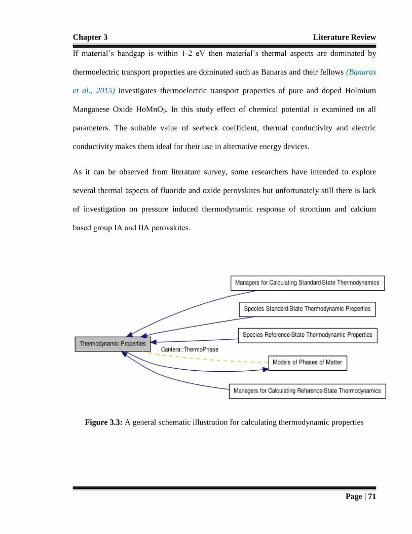
Chapter 3 Literature Review
Page | 71
If material’s bandgap is within 1-2 eV then material’s thermal aspects are dominated by
thermoelectric transport properties are dominated such as Banaras and their fellows (Banaras
et al., 2015) investigates thermoelectric transport properties of pure and doped Holmium
Manganese Oxide HoMnO3. In this study effect of chemical potential is examined on all
parameters. The suitable value of seebeck coefficient, thermal conductivity and electric
conductivity makes them ideal for their use in alternative energy devices.
As it can be observed from literature survey, some researchers have intended to explore
several thermal aspects of fluoride and oxide perovskites but unfortunately still there is lack
of investigation on pressure induced thermodynamic response of strontium and calcium
based group ΙA and ΙΙA perovskites.
Figure 3.3: A general schematic illustration for calculating thermodynamic properties

Chapter 3 Literature Review
Page | 72
3.8 Conclusion
The review of literature revealed that various perovskites have been widely investigated for
their structural, mechanical, opto-electronic and magnetic properties by number of
researchers but in spite of successful cases reported earlier, detailed physical aspects of many
oxide and halide perovskite are still under cover. Therefore, it is considered very important to
explore them for their possible applicability in various applications. This study could be
useful to provide new information regarding to behavior of alkali and alkaline based
fluoroperovskites, under different pressure and temperature conditions. Furthermore, another
purpose of this research is to develop an insight about significant properties of actinoid based
oxide perovskites for their possible technological benefits. The corresponding results are
presented in chapter 5 to 8, while the conclusion of the entire study is drawn in chapter 9.
Hopefully the present investigation will contribute towards scientific information on fluoride
and oxide perovskites for their structural, elastic, mechanical, electronic, optical, magnetic
and thermodynamic aspects under constant and variable temperature as well as pressure
conditions which would explore opportunities for material scientists to implement them in
numerous applications.

Chapter 4 Theory and Computational details
Page | 73
Chapter 4
Theory and Computational details
“All the mathematical sciences founded on relations
between physical laws and laws of numbers, so that the aim
of exact science is to reduce the problems of the nature to the
determination of quantities by operations with numbers”
James Clerk Maxwell
4.1 Introduction
To reinforce the trust of potential investors, technological development should be speed up
by involvement of researchers in competition of higher efficiencies. There are several ways
to investigate solution of a given research problem. Two major routes are theoretical work
and observational or experimental work. In the previous century a novel, third pillar of
research has been emerged which is an ab-initio or first principles investigation. The block
diagram representation of various theoretical methods is shown in Figure 4.1. The
requirement of ab-initio study lies to perform computational simulation because number-
crunching calculational power of computers have reached a critical mass so theoretically, the
only possibility to study the complex crystalline structure containing several atoms is to
perform computer simulations. Computational science and computational resources steadily
grew over the last few decades. Now-a-days simulation techniques are able to undertake
detailed and accurate calculations on an increasingly wide and complex range of materials
because microscopic description of physical and chemical properties is a complex problem.
They involve collection of interacting atoms which may be stimulated by external field.
These particles may be in gas to condensed phase, molecules or clusters, solids, surfaces,

Chapter 4 Theory and Computational details
Page | 74
wires or they can be molecules in solution, and adsorbates on surfaces (but in all cases, we
have to describe a system in terms of number of nuclei and electrons which are interacting
through electrostatic forces (Lejaeghere et al., 2013).
Computer simulations can be performed with variety of ways ranging from classical to
quantum mechanical approaches. The classical mechanical approach is based upon semi-
empirical scheme, which requires extensive input parameters in order to attain nearby
experimental results. While first-principles method based on quantum mechanical theories
allow the treatment of much smaller unit cell and do not require any experimental knowledge
as input to carry out such calculations. For the past 30 years, the quantum mechanical
simulation of the periodic systems has been dominated by density functional theory (Lany
and Zunger 2009).
In this chapter our focus is to describe the theoretical methods and approximate solutions
used in calculating physical properties of fluoride and oxide perovskites. The main purpose
of this chapter is to discuss background theories of computational methods used throughout
in this research work, covers bibliographic details of different exchange and correlation
schemes, which will briefly sketch computational elegance and simple conceptual framework
of ab-initio DFT studies.
4.2 Many body problems and Schrodinger wave equation
The microscopic description of the chemical and physical properties of the particles is a
complex problem. In general, ensemble of particles can be in variety of phases from gas
phase (clusters and molecules) to condensed phase (surface, solids, liquids, and wires) as
shown in Figure 4.2. In general, one of the major problems in condensed matter solid-state
physics is to determine ground state properties with a collection of N interacting atoms,

Chapter 4 Theory and Computational details
Page | 75
Figure 4.1: Block diagram representation of various theoretical methods (Weinberg 2013).
which may also be affected by external local potential provided by the nuclei. In quantum
mechanics, solution of such problems can be found in ground state wave function
|Ѱ(𝑟1, … , 𝑟𝑁)⟩ that holds all of the physical information about a system by solving time
independent Schrodinger equation (Schrodinger 1926) given as:
H|Ѱ⟩ = 𝐸 |Ѱ⟩ (4.1)
The expression for average total energy E is given by expectation value of Hamiltonian Ĥ
that is:
𝐸 = ⟨Ѱ|H|Ѱ⟩ (4.2)

Chapter 4 Theory and Computational details
Page | 76
Here the notation [Ѱ] corresponds that energy is a functional of wavefunction because it
takes function as input and gives number as output.
In equation 4.1 Ĥ represents Hamiltonian operator describing the N electrons of a system,
can be given by applying of well-known Born-Oppenheimer approximation (Born and
Oppenheimer 1927).
The purpose of this approximation is to decouple the entire system between two parts,
electronic part, and the nuclear part because mass of the nuclei is much greater than mass of
the electrons. For this reason, another name of Born-Oppenheimer approximation is
clamped-nuclei approximation. Hence, the complete Hamiltonian of many-body system can
be defined by sum of five terms given as:
H = Te + Tn +Ven +Vee +Vnn (4.3)
Here Te represents sum of kinetic energy operator of the electrons, Tn represents Kinetic
energy of nuclei, Ven represents electron-nuclei attractive interaction, Vee = electron-electron
repulsive interaction, Vnn = nuclei-nuclei repulsive interaction.
Detailed form of equation 4.3 can be written as:
H = =
−eN
em 1
22
2
=
−
nN
k k
k
m1
22
2
= = −
−e nN N
k k
k
Rr
eZ
1 1 0
2
||4 +
= −
e eN N
rr
e
1 0
2
||4 +
= −
n nN
j
N
jk kj
jk
RR
eZZ
1 0
2
||4
(4.4)
While i and j denote the N electrons in the system.
In general, the time independent Schrodinger wave equation 4.1 can be solved to attain
physical properties of a many body systems. However, practically it is not so easier because
within a given system each electron is influenced by potential of all other electrons, which
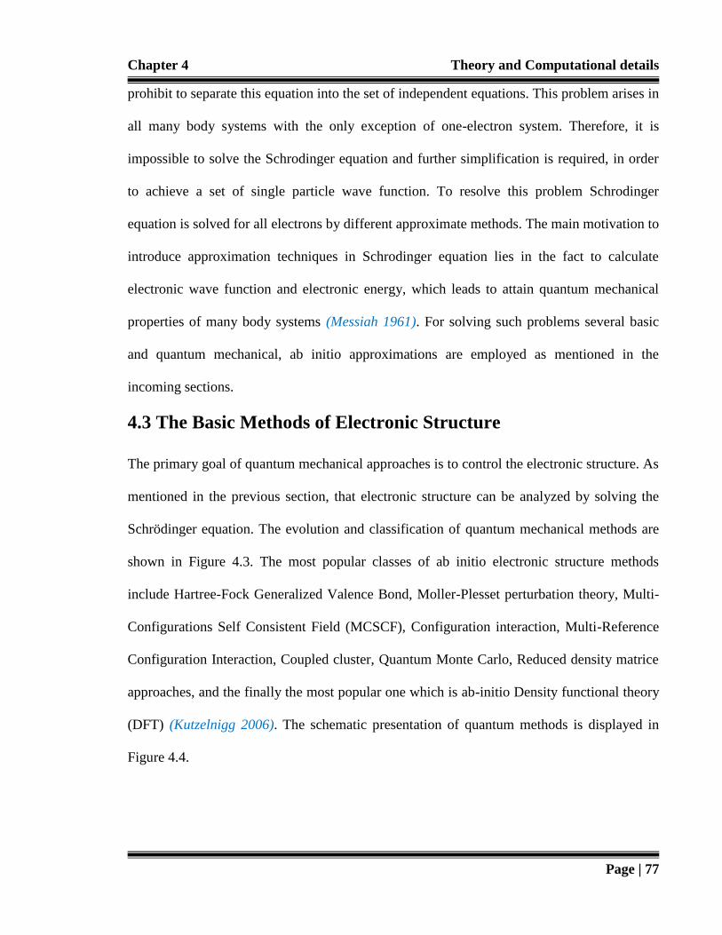
Chapter 4 Theory and Computational details
Page | 77
prohibit to separate this equation into the set of independent equations. This problem arises in
all many body systems with the only exception of one-electron system. Therefore, it is
impossible to solve the Schrodinger equation and further simplification is required, in order
to achieve a set of single particle wave function. To resolve this problem Schrodinger
equation is solved for all electrons by different approximate methods. The main motivation to
introduce approximation techniques in Schrodinger equation lies in the fact to calculate
electronic wave function and electronic energy, which leads to attain quantum mechanical
properties of many body systems (Messiah 1961). For solving such problems several basic
and quantum mechanical, ab initio approximations are employed as mentioned in the
incoming sections.
4.3 The Basic Methods of Electronic Structure
The primary goal of quantum mechanical approaches is to control the electronic structure. As
mentioned in the previous section, that electronic structure can be analyzed by solving the
Schrödinger equation. The evolution and classification of quantum mechanical methods are
shown in Figure 4.3. The most popular classes of ab initio electronic structure methods
include Hartree-Fock Generalized Valence Bond, Moller-Plesset perturbation theory, Multi-
Configurations Self Consistent Field (MCSCF), Configuration interaction, Multi-Reference
Configuration Interaction, Coupled cluster, Quantum Monte Carlo, Reduced density matrice
approaches, and the finally the most popular one which is ab-initio Density functional theory
(DFT) (Kutzelnigg 2006). The schematic presentation of quantum methods is displayed in
Figure 4.4.

Chapter 4 Theory and Computational details
Page | 78
Figure 4.2: Schematic chemistry of atoms and molecules in solids (Mitzi 1999).

Chapter 4 Theory and Computational details
Page | 79
Among them one of the most common type of an ab initio electronic structure approach is
called the Hartree-Fock (HF) method. D. R. Hartree and V. Fock proposed this
approximation scheme in 1930 (Hartree 1928 & Fock 1930). They attempted to solve many
body systems by using self-consistent field (SCF) approximation also known as Hartree-Fock
approximation which postulates that many-electron wave function can be written as a product
of one-electron wave function. The electronic wave function of N electron is approximated
by slater determinant, which fulfill the requirement that electrons satisfy Fermi-Dirac
statistics and Pauli Exclusion Principle. The exact form of approximation can be expressed as
Slater determinant matrix (Slater 1930):
Ѱ(𝑥1, 𝑥2, … 𝑥𝑁 ) = det (Ѱ1(𝑥1) … Ѱ1(𝑥𝑛). . .Ѱ𝑛(𝑥1) … Ѱ𝑛(𝑥𝑛)
) (4.5)
In equation 4.5 variational principle is applied to obtain minimum ground state energy. In
fact, it provides the way of choice to chemists for calculating the accurate atomic shell
structure with good description of inter-atomic bonding.
On a practical point of view, there are some major limitations in this theory because the
Hartree-Fock interaction neglects the electron correlation effect, which result to increase
repulsion energy of electrons, overestimating the ionic character and further influence on
band gap width and positioning of Fermi level especially in metals. It translates discrepancy
in some properties with respect to experimental measurements and for accurate results some
post-Hartree-Fock methods are required but they are computationally cost (Csavinszky 1968).
Many types of calculations such as Moller-Plesset perturbation theory (MP) and Coupled
Cluster (CC) begin with HF calculation and subsequently correct for the missing electronic

Chapter 4 Theory and Computational details
Page | 80
correlation. Another method which avoids making the variational overestimation in its
diffusion, variational, and Green's functions flavors in its first place is Quantum Monte Carlo
(QMC) (Onida et al. 2002). But these calculations can be very time consuming because these
methods work with an explicitly correlated wavefunction and evaluate integrals numerically
using a Monte Carlo integration. In order to overcome limitations in basic methods to
determine electronic structure, an alternative theory well known as Density Functional
Theory (DFT) is introduced which has been applied extensively in this thesis work.
4.4 The Density Functional Theory (DFT)
“Is simplicity best,
Or simply the easiest?
Martin L.Gore
Density Functional Theory (DFT) is a quantum mechanical ground state approach in which
emphasis is on the use of electrons charge density instead of electronic wave function. DFT
has proved to be highly successful tool for the calculation of many physical properties like
structural, elastic, electronic, mechanical, magnetic optical, thermal, thermodynamic, and
thermoelectric properties of metals, semi-metals, half-metals, semiconductors, conductors,
superconductors and insulators covering all types of bulk substances and nanostructures.
DFT is extensively used in various research areas of chemistry and physics because of its
computational simplicity. In fact, DFT is an operationally independent-particle theory
(Kohanoff and Gidopoulos 2003).

Chapter 4 Theory and Computational details
Page | 81
Figure 4.3: The evolution and classification of quantum mechanical methods (Griffiths
2004).

Chapter 4 Theory and Computational details
Page | 82
Figure 4.4: Schematic presentation of Quantum methods.
Figure 4.5: A schematic representation of the relationship between the "real" many body
system (left hand side) and the non-interacting system of Kohn Sham density functional
theory (right hand side) (Lany and Zunger 2009).
QUANTUM METHODS
Wavefunctions
Basic methods
Electron density
Modern DFT

Chapter 4 Theory and Computational details
Page | 83
Although DFT has its theoretical roots in the Thomas-Fermi model but it was put on a solid
hypothetical foundation by Walter Kohn (who worked out the theory) and John Pople (who
implemented the theory) they combinedly proposed the concept of modern DFT. In
recognition to importance of this theory, both scientists were awarded with the chemistry
Noble Prize in 1998. The main idea behind DFT is to describe a fermion interacting system
via its charge density instead of its many body wave function which reduces 3N variables of
N particles to three variables of density, ρ (x, y, z,) (Suryanarayana et al., 2010). This theory
can be best described within framework of Hohenberg-Kohn theorems and Kohn-Sham
equations.
4.5 Hohenberg-Kohn Theorems and Kohn Sham Equations
The basics of DFT lie in two fundamental theorems proposed by Hohenberg and Kohn in
1964 (Hohenberg and Kohn 1964). They gave mathematical proof of the concept that the
energy of a system can only be defined in terms its electron density. This long mathematical
proof was explained in terms of two theorems discussed in this section and schematic
representation is shown in Figure 4.5, in which left hand side represents the relationship
between the real many body system and right-hand side represents the non-interacting system
of Kohn Sham density functional theory.
The Hamiltonian of the system can be best described by following equation:
�� = �� + �� + �� (4.6)
In equation 4.6, the first term is due kinetic energy, the second term represents electron-
electron interaction, and the third term introduces electron interaction with nuclei and
external potential.

Chapter 4 Theory and Computational details
Page | 84
According to the first theorem (Martin 2004) for any system of interacting particles, the
external potential V(ṟ) is uniquely determined, except for a constant, by the electronic density
n(r). Then the Hamiltonian operator uniquely determined corresponding ground state
stationary wave function |Ѱ[𝑛]⟩ and all underlying properties of the many body systems. In
this way electron-electron, interaction energy, and kinetic energy can be expressed by the use
of the density. However, this theorem gives no information how one can calculate the density
of a system, which is proposed in the second theorem.
The second theorem (Kohanoff and Gidopoulos 2003) shows that in case of any particular
external potential V(ṟ), the accurate electron density is global minimum value of the ground
state energy functional, in short density obeys variational principle. The contribution of
expectation value can be expressed as functionals of 𝜌(ṟ). So, we therefore have:
𝐸𝑔[𝜌(ṟ)] = ∫ 𝑉(ṟ)𝜌(ṟ)𝑑ṟ + 𝐹[𝜌(ṟ)] (4.7)
Where 𝐹[𝜌(ṟ)] represents kinetic energy of electrons and mutual interaction between them,
V is the potential and 𝜌 is the density of electrons.
𝐹[𝜌(ṟ)] can be broken down into two parts:
𝐹[𝜌(ṟ)] = 𝑇[𝜌(ṟ)] + 𝑈[𝜌(ṟ)] (4.8)
In equation 4.8 𝑇[𝜌(ṟ)] represents influence of kinetic energy of a non-interacting electronic
system whose distribution is 𝜌(ṟ) and electron-electron interaction energy of a system is
given by 𝑈[𝜌(ṟ)], where𝐹[𝜌(ṟ)], denotes universal functional, for this functional a
variational principle hold, which is valid for any external potential with finite number of
particles. For a known 𝐹[𝜌(ṟ)], within a given potential, the evaluation of ground state

Chapter 4 Theory and Computational details
Page | 85
energy and density will be easy. Therefore, the expression for total energy whose distribution
is 𝜌(ṟ) can written as:
𝐸𝑡𝑜𝑡[𝜌(ṟ)] = ∫ 𝑉(ṟ)𝜌(ṟ)𝑑ṟ + 𝑇[𝜌(ṟ)] + 𝑈[𝜌(ṟ)] (4.9)
As mentioned previously that 𝑇[𝜌(ṟ)] is the kinetic energy, it cannot be minimized with
reference to 𝜌. So Kohn-Sham proposed an indirect method for total energy minimization by
using the Lagrange multiplier to constrain the number of electrons given as:
𝛿𝐸𝑡𝑜𝑡
𝛿𝜌(ṟ)= 𝑉(ṟ) +
𝛿𝑇[𝜌(ṟ)]
𝛿𝜌(ṟ)+
𝛿𝑈[𝜌(ṟ)]
𝛿𝜌(ṟ)= 𝜇 (4.10)
Kohn and Sham demonstrated that how the properties of a homogenous gas can be applied in
the theoretical investigation of inhomogeneous system.
The potentials in equation 4.10 can be collected by introducing an effective potential 𝑣𝑒𝑓𝑓 :
𝑣𝑒𝑓𝑓 = 𝑉(ṟ) +𝛿𝑈[𝜌(ṟ)]
𝛿𝜌(ṟ) (4.11)
By using above equation, the equation 4.10 can be written as:
𝛿𝑇[𝜌(ṟ)]
𝛿𝜌(ṟ)+ 𝑣𝑒𝑓𝑓(ṟ) = 𝜇 (4.12)
Where 𝜇 is a constant, which represents chemical potential. So, for a system of non-
interacting electrons the expression for total energy can be written as:
𝐸𝑡𝑜𝑡[𝜌(ṟ)] = ∫ 𝑉(ṟ)𝜌(ṟ)𝑑ṟ + 𝑇[𝜌(ṟ)] +𝑒2
8лє0∬
𝜌(ṟ)𝜌(ṟ)
|ṟ−ṟ|𝑑ṟ𝑑ṟ + 𝐸𝑋𝐶[𝜌(ṟ)] (4.13)
In equation 4.13 the last term 𝐸𝑋𝐶[𝜌(ṟ)] denotes exchange correlation energy, functionally
depending on the entire density distribution 𝜌(ṟ) which contains all terms whom exact

Chapter 4 Theory and Computational details
Page | 86
solution is unknown. (In next section, it will discuss in detail). The method developed by
Khon-Sham, proposed a practical solution of DFT equation by introducing a one-electron
Hamiltonian like Schrodinger equation, in the following manner:
−ħ2
2𝑚𝛻2Ѱ𝑛(ṟ) + 𝑣𝑒𝑓𝑓(ṟ)Ѱ𝑛(ṟ) = є𝑛Ѱ𝑛(ṟ) (4.14)
Where −ħ2
2𝑚𝛻2 (non-relativistic approximation) denotes Kinetic energy operator and the
resulting total electron density is given by:
𝜌(ṟ) = ∑ |Ѱ𝑛(ṟ)|2𝑛 (4.15)
In summary, 𝑣𝑒𝑓𝑓 can be calculated from an initial guess of density, which can further put
into equation 4.14 to attain є𝑛Ѱ𝑛(ṟ) and used to calculate a new density. The contribution of
DFT is to provide a precise prescription to determine effective potential (𝑣𝑒𝑓𝑓) for
calculating the total ground state energy.
The mathematical framework for finding ground state density is taken from Kohn-Sham
equations, which utilizes standard independent particle methods. As shown schematically in
Figure 4.6 that these equations can be solved self-consistently. It consists of following steps:
1. An initial guess of electron density 𝜌(ṟ), is generated.
2. Then it is used to calculate effective potential𝑣𝑒𝑓𝑓(ṟ).
3. Which can further put into equation 4.14 to attain є𝑛Ѱ𝑛(ṟ) and used to calculate a
new density 𝜌𝑜𝑢𝑡.
4. This process is repeated until self-convergence is achieved, within a chosen numerical
accuracy i.e. 𝜌𝑜𝑢𝑡(ṟ) = 𝜌𝑖𝑛(ṟ) (Dreizler et al., 1990).

Chapter 4 Theory and Computational details
Page | 87
Figure 4.6: Schematic description of the SCF cyclic procedure in solving the Kohn-Sham
equations (Blaha et al., 2008).

Chapter 4 Theory and Computational details
Page | 88
4.6 The Exchange and Correlation approximations
The main challenge of modern DFT is to achieve the balance between accuracy of practical
calculation and computational cost. For this purpose, several approximations have to be
introduced because in Kohn-Sham equations, exchange-correlation energy 𝐸𝑋𝐶[𝜌(ṟ)]
functional is the only unique term. It is the minimum energy for all possible many-body wave
functions within the given density. The phenomenon of exchange-correlation energy 𝐸𝑋𝐶 or
exchange-correlation potential describes the fact of Coulomb potential and Pauli Exclusion
Principle beyond the pure electrostatic interaction because electrons being fermions, require
their wave functions to be anti-symmetric when two electrons are interchanged (Parr and
Yang 1989). The generation of Exchange and Correlation approximations have emerged
novel innovations in the field of DFT research.
4.6.1 The Local Density approximation (LDA)
The first and simplest approximation, has been proposed in the seminal paper, by Kohn and
Sham, is known as Local Density Approximation (LDA). For a long time, the LDA has been
the most widely used approximation for the exchange-correlation energy in density
functional theory (DFT) (Pople et al., 1992). The LDA method uses exchange correlation
energy density calculated from uniform electron gas to measure the exchange energy. This
scheme has been widely used to portray a varied range of exchange-correlation interactions
in covalently bonded systems but these functionals cannot identified accurately and they
must be calculated approximately. LDA the simplest approximation is known to be local in
the sense that at any point in the space corresponding electron exchange and the correlation
energy is a function of electron density at that point only. Within this approximation, the

Chapter 4 Theory and Computational details
Page | 89
expression for total exchange- correlation energy is approximated as integral of all
contributions. Thus:
𝐸𝑋𝐶𝐿𝐷𝐴[𝜌(ṟ)] = ∫ є𝑋𝐶
𝐿𝐷𝐴[𝜌(ṟ)] 𝜌(ṟ)𝑑ṟ (4.16)
Where є𝑋𝐶𝐿𝐷𝐴[𝜌(ṟ)] is the exchange-correlation energy density of the real non-uniform
electron gas.
In case of magnetic systems, where the spin also plays a vital role while involving open
electronic shells in the properties of a material; better approximations to exchange-
correlation functional can be obtained by introducing the effect of up and down spin densities
in LDA approximation and named as Local Spin Density Approximation (LSDA). In LSDA,
the exchange and correlation contribution are separated as (Wu and Cohen 2006):
𝐸𝑋𝐶𝐿𝐷𝐴[𝜌 ↑ (ṟ), 𝜌 ↓ (ṟ) ] 𝜌(ṟ) = ∫ є𝑋𝐶
𝐿𝐷𝐴[𝜌 ↑ (ṟ), 𝜌 ↓ (ṟ) ] 𝜌(ṟ)𝑑ṟ (4.17)
Where є𝑋𝐶𝐿𝐷𝐴[𝜌 ↑ (ṟ), 𝜌 ↓ (ṟ) ] is the exchange-correlation spin-polarized energy density of the
real non-uniform electron gas.
In fact, in the LDA scheme 𝐸𝑋𝐶𝐿𝐷𝐴[𝜌(ṟ)] is function of the local density, which can be easily
separated into exchange and correlation parts such as:
𝐸𝑋𝐶𝐿𝐷𝐴[𝜌(ṟ)] = 𝐸𝑋
𝐿𝐷𝐴[𝜌(ṟ)] + 𝐸𝐶𝐿𝐷𝐴[𝜌(ṟ)] (4.18)
Similarly, for LSDA:
𝐸𝑋𝐶𝐿𝐷𝐴[𝜌 ↑ (ṟ), 𝜌 ↓ (ṟ) ] = 𝐸𝑋
𝐿𝐷𝐴[𝜌 ↑ (ṟ), 𝜌 ↓ (ṟ) ] + 𝐸𝐶𝐿𝐷𝐴[𝜌 ↑ (ṟ), 𝜌 ↓ (ṟ) ] (4.19)
The significant point that proves this system easier to solve is that it reduces the energy
functional to a local function of the density. Hence no more complication added in solving

Chapter 4 Theory and Computational details
Page | 90
Schrodinger’s equation. The properties such as phase stability, vibrational frequencies,
charge moments, and elastic moduli can calculate with accuracy.
Despite of its accuracy LDA as well as LSDA have some shortcomings. Typical error ratio
with respect to experimental value is about 1% on atomic positions and of about 5% for
phonon frequencies. In LDA and LSDA schemes exchange-correlation energy density
depends only on local potential while it should be non-local, which means it should depends
on the system at every point in the space. LDA retains problems for highly localized and
strongly correlated electrons like compound of rare-earth elements and transition metal
oxides. One of the serious limitation of LDA include that it cannot be able to provide
estimation for long-ranged exchange interaction such as Van der Waal’s interaction. This
type of interaction is long ranged (electronic interaction) which mainly add in primary stage
of material development and in reactions such as crystal growth, chemical stability and
physical absorption. LDA have another serious limitation that in atoms bond energy
calculations are not accurate where the electrons are quite localized and the electron densities
are poor. In this way, ground state energies of atoms are underestimated and binding energies
are overestimated. In addition, the local structure of the energy expression does not justify
electronic arrangement in bonds that excludes chemistry from the functional expression
(Ceperley and Alder 1980).
4.6.2 The Generalized Gradient approximation (GGA)
For certain systems LDA works well but it fails for other materials due to several reasons,
one of them is that the distribution of electrons within a molecule is not uniform. The next
generation of functional have aimed for treating inhomogeneous electron system including

Chapter 4 Theory and Computational details
Page | 91
the gradient of density into locally expanded functional. This type of functional has attracted
much attention due to its abstract simplicity and moderate computational workloads. In
general, this relation can be expressed as (Wu and Cohen 2006):
𝐸𝑋𝐶𝐺𝐺𝐴[𝜌(ṟ)] = ∫ є𝑋𝐶
𝐺𝐺𝐴[𝜌(ṟ)] 𝜌(ṟ)𝐹𝑋𝐶[𝜌(ṟ), 𝛻𝜌(ṟ), 𝛻2𝜌(ṟ), … . ]𝑑ṟ (4.20)
Here 𝐹𝑋𝐶 is the factor, which use to modify the LDA functional in order to consider the
variation of 𝜌(ṟ) at the reference point and which is asked to satisfy a number of formal
conditions for the exchange-correlation hole, long range decay, sum rule and so on. The
approximation of this type is known as Generalized Gradient Approximation (GGA).
GGA type of functionals are often referred to as functional zoo because a very large number
of functionals have been proposed. What is needed for the functional is a from that mimics a
re-summation to infinite order, however for GGA there is not unique recipe. A through
comparison of different GGA functionals are done by Filippi and his fellows (Filippi et al.,
1994). These functionals may vary from parameter to parameter. Naturally, not all the formal
properties can be enforced at the same time, and differentiates one functional from other such
as while the functionals that contain second derivative of charge density (to improve
accuracy of kinetic energy functional) are called meta-GGA. Some of the renowned GGA
functionals includes Lee, Yang and Parr’s correlation functional (LYP) (Miehlich et al.,
1989), Becke’s exchange function (B88) (Becke 1988), Perdew, Burke and Ernzerhof’s
exchange-correlation functional (PBE) (Perdew 1996), Perdew and Wang’s (PW91)
correlation functional (Perdew and Wang 1992), Wu and Cohen (WC) density gradient
functional (Wu and Cohen 2006) are worthy to mention.

Chapter 4 Theory and Computational details
Page | 92
In GGA functionals higher order expansion in equation 4.20 have been developed but it will
lead to violate some suitable conditions for exchange and correlation as showed by Perdew
(Perdew 1986) that originally did not yield any notable improvement in the exchange
energies and analytical equation for the potentials become highly complicated. Despite of the
fact, these functionals may not necessarily base on new physical ideas but GGA functionals
yields better results than the LDA because different LDAs modeling the electron gas yield
nearly identical results, different GGAs can yield very different energetic and structural
results because of the freedom in the parameters of the gradient expansion.
In general, GGA methods can improve the computed binding energies, electron affinities,
atomic energies and give better representation for non-uniform densities over the LDA.
According to report of Perdew (Perdew 1986) GGA exhibits an error of 1 % while LDA has
14% error in the calculation of exchange correlation energies. Many calculations assessing
the accuracy of GGA demonstrates that it substantially corrects the LDA error in the
cohesive energies of solids and molecules.
Despite of its accuracy GGA have some shortcomings. The lattice parameters by GGA
always rise in comparison with LDA, however a close agreement with experimental data is
observed for alkali 3d and 4d metals. For molecules thermos-chemistry GGA schemes also
delivers poor results. Similarly, for opto-electronic calculations GGA underestimates these
results, for instance the theoretical bandgap of AlN in zinc blende structure is 4.2 eV
(Litimein et al., 2002) and 5.40 eV (Amin et al., 2011) by LDA and GGA schemes
respectively while the calculated value of experimental bandgap is of 6.2 eV (Martinez et al.,
2001). The same problem arises for almost all kind of compounds. Unlike LDA, GGA
functionals are not unique. These functionals cannot be classified as purely ab-initio

Chapter 4 Theory and Computational details
Page | 93
calculation because some experimental data is required to solve parameters in GGA
functional. However, performance may vary from type of material under investigation. In
comparison with experimental results GGA scheme has some limitations. Hence for attaining
good results researchers in this field are aiming to get their results close to experimental
values so they use different flavors of LDA and GGA for strongly correlated systems like
LDA+U and GGA+U (Anisimov et al., 1997).
4.6.3 The modified Becke–Johnson (mBJ) potential
In majority solid state calculations, determination of electronic structure is done with Kohn-
sham equations by using various approximations such as local density and generalized
gradient approximations for exchange correlation energy as well as for potential. But in many
circumstances these local or semi local approximations cannot be able to interpret accurate or
enough experimental data. The calculated values of bandgap for LDA and GGA schemes
underestimates the bandgap because of the fact that GGA as well as LDA schemes
undervalues bandgaps in semiconductor as well as insulators. The wrong interpretation of the
true unoccupied states with respect to corresponding Khon–Sham DFT states, results this
underestimation (Grabo et al. 1997).
Tran and Blaha in 2009 (Tran and Blaha 2009) tested and verified modified Becke and
Johnson (mBJ) potential for accurate bandgap calculations of sp-semiconductors, wide
bandgap insulators and for strongly correlated 3d transition-metal oxides. This newly
developed scheme minimizes the conflict between the theoretical and experimental
investigations. It is an exchange potential which used to handle exchange and correlation

Chapter 4 Theory and Computational details
Page | 94
energy for strongly correlated electron systems (Koller et al., 2011). It was proposed by
following expression:
𝑈𝑋,𝜎𝑀𝐵𝐽(𝒓) = 𝐶𝑈𝑋,𝜎
𝐵𝑅 (𝒓) + (3𝐶 − 2)1
𝜋√
5
12 √
2𝑡𝜎(𝒓)
𝜌𝜎(𝒓) (4.21)
where 𝑡𝜎 =1
2∑ (𝛻Ѱ𝑖,𝜎
∗ ). (𝛻Ѱ𝑖,𝜎)𝑁𝜎𝑖=1 is the kinetic energy density, 𝜌𝜎 =
1
2∑ |Ѱ𝑖,𝜎|
2𝑁𝜎𝑖=1 is the
density of the electron, while the Becke-Russel potential is given by (Becke and Johnson
2006):
𝑈𝑋,𝜎𝐵𝑅 (𝒓) = −
1
𝑏𝜎(𝒓)(1 − 𝑒−𝑥𝜎(𝒓) −
1
2𝑥𝜎(𝒓)𝑒−𝑥𝜎(𝒓)) (4.22)
and C in equation 1 can be elaborated by:
𝑐 = 𝑎 + 𝑏√1
𝑉𝑐𝑒𝑙𝑙∬
|𝛻𝜌(𝒓)|
(𝜌(𝒓))𝑐𝑒𝑙𝑙𝑑3𝑟 (4.23)
In the above equation Vcell is the unit cell volume where a and b are two independent
parameters, with the values of -0.012 (dimensionless) and 1.023 Bohr1/2, respectively.
In fact, mBj is an exchange correlation, not exchange correlation functional so first one has
to use modern LDA or GGA approximation for structural properties and then to use
mBJLDA or mBJGGA potential for the proper calculations of the corresponding band
structure. In fact, the Becke and Johnson (BJ) potential can either be used in combination
with LDA or GGA (Perdew and Wang 1992), and that can be termed as mBJLDA or
mBJGGA. These potential leads to more sophisticated results with more demanding
computational orders of magnitude. As a result, a very accurate bandgap specially of wide
bandgap semiconductors and insulators can be obtained. This is a type of semi local potential
which can compete in accuracy with other expensive hybrid methods. So, it can be efficiently
applied to large systems which was certainly not possible with other hybrid methods.

Chapter 4 Theory and Computational details
Page | 95
The Tran-Blaha functional have attracted a lot of interest recently due to the accurate
predictions of the band gaps in semiconductors and insulators and the low-computational
cost. However, this functional has also some drawbacks which should be emphasized e.g. the
TB-mBJ functional is not a functional derivative and cannot be used to calculations of forces,
lattice constants, phase stability etc (Koller et al., 2011). For cubic perovskites without
strongly localized f- or d-states the TB-mBJ functional gives similar results to the
computationally more expensive hybrid HSE functional (Kaczkowski and Jezierski 2013).
However, for localized states better agreement with experimental results is obtained within
LDA+U approach. There are some limitations and some benefits in these theoretical schemes
but their selection can be based upon selection of system under consideration.
4.7 Methods for solution of Kohn Sham Equations
There are several techniques to solve DFT Kohn Sham equations, once they are described
into functional terms. Nowadays different codes are available in the simulation market that
can solve these equations with ease but they can differentiate in terms of basis sets. The
different basis sets used are in actual the linear combination of atomic orbitals (abbreviated
as LCAO), Slater type or Gaussian orbitals (abbreviated as STOs, GTOs), plane wave
(abbreviated as PW) with or without augmentations, Linearized Augmented Plane Wave
(abbreviated as LAPW) with or without Local Orbitals, and muffin tin orbitals (abbreviated
as MTOs). The wave functions, which represent these basis sets, can be all-electron wave
functions or pseudo-wave functions (Patterson et al., 2010). However, calculations in this
thesis have been based upon Full-Potential Linearized Augmented Plane Wave Method (FP-
LAPW) which is integrated into Wien2k Package of simulation software (Schwarz et al.,
2010).

Chapter 4 Theory and Computational details
Page | 96
4.8 Full-Potential Linearized Augmented Plane Wave Method
(FP-LAPW)
To solve one-electron Kohn-Sham equation in terms of Khon-Sham orbitals, one of the most
reliable methods is the Full-Potential Linearized Augmented Plane Wave Method (FP-
LAPW) which allows most precise calculation of the electronic structure and other physical
quantities of crystals and surfaces. The use of this technique depends upon binding strength
of electrons in solids which leads to maximize its applicability in atomic forces. The muffin
tin Augmented Plane Wave (APW) and Linearized Augmented Plane Wave (LAPW)
approaches were frequently used in the era of 1970s. In these methods, potential is assumed
constant in the interstitial region and symmetrically spherical in the muffin-tin region. These
approximations are highly useful in order to explain the metallic systems but not very
efficient in the calculation of structure and opto-electronic parameters of open structured as
well as covalently bonded solids. A comprehensive description of three types of schemes
APW, LAPW, APW+lo is explained in detail by Schwarz (Schwarz et al., 2010). To
overcome these limitations and to obtain better predictions for these properties, the non-
muffin tin approximation (no shape approximation) were applied which is named Full-
Potential Linearized Augmented Plane Wave Method (abbreviated as FP-LAPW) but indeed
FP-LAPW computation need considerable higher computational effort in comparison with
the pseudopotential plane wave (PPW) based methods. The FP-LAPW method combines the
basis of LAPW with full potential treatment to solve the Kohn-Sham equations for the
ground state total density, ground state total energy, and eigenvalues of many body electron
system by introducing finite set of basis. In this approach unit cell potential, and charge
density are expanded by linear combinations of lattice harmonics inside the atomic sphere.

Chapter 4 Theory and Computational details
Page | 97
This alteration is achieved by partitioning the unit cell as shown in Figure 4.7 into (Ι) non-
overlapping atomic circles; centered at atomic sites and (ΙΙ) outside the sphere an interstitial
region; region between two spaces (Madsen et al., 2001). Another pictorial representation of
unit cell division is displayed in Fig. (3.7). The FP-LAPW method extends the potential
inside and outside the sphere in the following from:
𝑉( 𝑟) = ∑ 𝑉𝐿𝑀𝐿𝑀 (𝑟)𝑌𝐿𝑀(𝑟) Inside sphere (4.24)
𝑉( 𝑟) = ∑ 𝑉𝐾 𝐿𝑀 𝑒𝑖��.�� Outside sphere (Interstitial region) (4.25)
where the equation 4.24 is for inside the sphere and equation 4.25 is for outside or interstitial
region of the atomic sphere. These non-muffin tin corrections do not affect the choice of
basis functions in the interstitial regions but by using true crystal potential, the radial wave
functions are evaluated. So, the benefit of FP-LAPW method is that it is free in selection of
sphere radii as compared to old APW as well as LAPW methods. The effects for relativistic
valence states can be either incorporated in scalar relativistic handling or with the second
dissimilarity technique including spin-orbit coupling. Furthermore, in FP-LAPW method the
core states are computed self-consistently by using the spherical part of the crystal potential
within Muffin Tin (MT) spheres. Potential is spherically symmetric inside the sphere while it
is constant outside the sphere. However, eigenstates and eigenvalues treatment of core
electrons is fully relativistic and it is semi-relativistic for the valence electrons. The union of
basis set in FP-LAPW method is controlled by a disconnect parameter RMT х Kmax, where
RMT is the smallest atomic sphere radius in the unit cell and Kmax is the magnitude of the
corresponding largest K vector.

Chapter 4 Theory and Computational details
Page | 98
Recently FP-LAPW method has showed important progress. Now-a-days researchers are
working out on several nuclear and magnetic quantities using FP-LAPW method such as
isomer shifts, electric field gradients, hyperfine fields, and core level shifts. The recent
optimization has significantly reduced the CPU time of these calculations. However, FP-
LAPW implementations are fairly suitable for complicated systems, because of its
computational expense and memory requirements. One successful implementation of this
technique is simulation program package of WIEN2K discussed in the coming section.
4.9 Simulation techniques
First principle calculations have been the foremost and modern tool to achieve theoretical
understanding and prediction of physical properties, kinetic and thermally driven
phenomenon which otherwise are beyond the reach of several other computational
techniques. In this field variety of computer codes are available such as VASP (Parlinski and
Kawazoe 2000), CRYSTAL code (Piskunov et al., 2004), SIESTA code (Coulaud et al.,
2013), Quantum Espresso (Giannozzi et al., 2009), ABINIT code package (Roy et al., 2010),
CASTEP code (Segall et al., 2002), FEFF (Rehr et al., 2013), Lmtart computer code
(Savrasov et al., 2004), CP2K (Carignano et al., 2014) but in this thesis attention is paid to
WIEN2k code (Schwarz et al., 2010 & Erum and Iqbal 2016) due to its various features such
as graphical user interface, low convergence time, accuracy, efficiency, user friendliness,
robustness & portability.

Chapter 4 Theory and Computational details
Page | 99
Figure 4.7: Partitioning of the unit cell into atomic spheres (I) and an interstitial region (II)
(Blaha et al., 2002).
Figure 4.8: The unit cell divided into muffin-tin region and interstitial region
(Schwarz et al., 2010).

Chapter 4 Theory and Computational details
Page | 100
4.9.1 The WIEN2k Package
Almost all computational work presented in this thesis on oxide and halide perovskite
compounds has been performed by using WIEN2K code (Blaha et al., 2008). This code is
embedded in the framework of density functional theory. Its development brings computation
of various material properties such as structural, chemical, opto-electronic, mechanical,
thermal, and magnetic by structure generation of periodically arranged unit cells at absolute
zero. The calculation of aforementioned properties can be done by applying different
physical laws within framework of density functional theory.
Over a period of more than twenty years, a full-potential LAPW method has been developed
for crystalline solids but its copyrighted first version was called named as WIEN (Blaha et
al., 1990). In succeeding years significantly, improved UNIX based versions of WIEN were
WIEN93, WIEN95 and WIEN97 but based on alternative basis set newly updated version is
WIEN2k (WIEN2k_16.1) which is LINUX based and written in many independent
FORTRAN 90 programs. The sequences of individual modules are linked together through
C-shell scripts alongwith F90 compiler. The WIEN package contains several sub-programs.
The WIEN developers have the strategy to provide a general code with the help of these sub
programs.
Major steps to evaluate crystalline properties includes generation of structure followed by
space group selection of the chosen material with suitable lattice coordinates. In the next
step, initialization of the code is done through step by step process which ultimately detects
minimum separation energy required to stabilize the unit cell structure. Then finally SCF
calculations are performed. The flow chart of WIEN2k code SCF cycle in single mode and in

Chapter 4 Theory and Computational details
Page | 101
parallel mode is shown in Figure 4.9. The two major parts in program flow of WIEN2K are
initialization and the self-consistent field (SCF) cycle. The purpose of initialization step is to
generate the unit cell and set up the initial density. The construction of the effective potential
is done with the help of LAPW0 program. Then the program LAPW1 solves the Khon-Sham
equation for valence electrons. The construction of new electron density is done with the help
of LAPW2. The LCORE program treats the core electrons. Finally, the input density for the
next iteration is done with LMIXER program. In current platform of WIEN2k core states has
flexibility to describe atomic-like states near the nuclei and electron-like states in the
interstitial.
The all electron nature of WIEN2K means it calculates all electron states including explicitly
the tightly bound, atomic like deep core states (Laskowski et al., 2004). It is an Augmented
Plane Wave Plus Local Orbitals (APW+lo) Program for calculating crystal properties and
allows major upgrading particularly related to speed, universality, and user accessibility
(Blaha et al., 2002).WIEN2k can treat all atoms of periodic table in similar manner such as
from heavy atoms like U to lighter atoms like C in similar manner and this balance is due to
mixed basis set of plane waves and atomic functions while solving radial Dirac equation
numerically for each SCF iteration. This allows them to expand or contract according to their
potential. Besides all these specifications, WIEN2k code is one of the fastest and consistent
simulation codes among to calculate crystalline properties at atomic level. Almost all
computational work presented in this thesis on oxide and halide perovskites are done using
WIEN2k code which is embedded in the framework of Density functional theory. In fact,
there are some limitations in this code and to improve that several bugs are adding on daily

Chapter 4 Theory and Computational details
Page | 102
basis in this code and hope can be generated that future WIEN2K will be much better than
present WIEN2K.
Figure 4.9: Flow chart of WIEN2k code SCF cycle in single mode and in parallel mode
(Schwarz et al., 2010).
4.10 Applications of Density functional theory (DFT)
Density functional theory (DFT) has made an unparalleled impact on the application of
quantum mechanics and challenging problems in condensed matter physics. It is a subtle,
provocative, and seductive business in the field of theoretical research. It can drive one mad
due to its basic premise that all the intricate motions and pair correlations in many electron
systems are contained by total electron density alone. This theory provides an unbiased tool
to compute the ground state energy in relatively realistic models of bulk materials and
surfaces. The reliability of such calculations is based upon accurate approximations to

Chapter 4 Theory and Computational details
Page | 103
exchange-correlation functional. It can be applicable to simple as well as complex systems
such as atoms, molecules, 3d solids, 2d surfaces and interfaces. Density functional theory
(DFT) has been immensely successful in its ability to predict physical properties, and, in
particular, structures of condensed matter systems. It can investigate atomic and molecular
structures, the understanding and design of catalytic, ionization potentials, vibrational
spectra, chemical reactions in biomolecules, nature of active sites in catalysts, phase
transition in solids, bond length, bond strength, liquid metals, and properties of magnetic
materials, processes in enzymes and zeolites, electron transport, solar energy, harvesting and
conversion, drug design in medicine, as well as many other problems in science and
technology. The story behind the success of DFT over Hartree-Fock (H-F) is hidden in its
electron correlation energy, which is generated by the interaction of pair for electrons. The
consideration of correlation energy in HF method is required by Pauli repulsion energy
(Martin 2004).
One of the advantage of DFT lies in the phenomenon of electron correlation which is the
major reason for localization and delocalization of electrons in a system. For example, for
solids LDA approximation turns out to be computationally much more successful than HF
due to true exchange potentials and slightly simpler Slater’s local exchange approximation.
Another significant advantage of DFT is due to its reduced cost over HF method (Zieger
1991) because DFT calculations scales to N3 while HF calculations scales to N6 where N
represents number of electrons in a system. It means that larger simulation cells can be
simulated using DFT for the same computational cost (Gill 1992).
An interesting aspect of DFT is that even the simplest systems can show details and
challenges reflecting those of much larger and complex systems. One example of this is the

Chapter 4 Theory and Computational details
Page | 104
understanding of the extensively used term, “strong correlation.” In literature, strong
correlation is meant to mention the breakdown of the single-particle picture, which is based
on a determinant of single particle Kohn Sham orbitals. The Strongly correlated systems
offer significant and new challenges for the functional. The challenge to demonstrate strong
correlation for density functionals can help to realize the enormous potential of DFT (Lany
and Zunger 2009).
Despite the applications and successes of DFT in many branches of science and engineering,
there are some future challenges and known issues for DFT. DFT detractors complain about
the prerequisite of KS-DFT, that the exchange-correlation functional should be exact, then
quantum mechanical nature of matter can be described correctly by DFT. In fact, it is the
approximate nature of the exchange correlation functional that is the reason both for the
success as well as for the failure of DFT applications because exchange-correlation
functional and its underlying hole will never be expressible in closed analytical form, which
made DFT heaven probably, be unattainable. This leads to major limitation of standard DFT
in describing strongly correlated systems. DFT computations in all known implementations
are found to qualitatively break down into certain strongly correlated electron systems,
sometimes it predicts a compound to be a metal while experimentally it is an insulator. This
problem is known as self-interaction error. In real system, each electron is under influence of
every other electron other than it-self while in DFT all electrons are described by coulomb
interaction with all others and with themselves through Hartree term. Therefore, the term
“self-interaction” referred as Coulomb interaction of one electron with its own electron
density. When electrons interact with it-self, they affect the modeling of charge localization,
magnetic materials, and superconductivity. To remove this limitation, there are several ways
Chapter 4 Theory and Computational details
Page | 105
to correct this error, with the commonly used self-interaction correction (SIC) or through
using DFT+U (Szabo and Ostlund 1982). So new and deeper theoretical insights are needed
to aid the development of new functionals. Another problem in DFT is incorrect description
of cohesive energy of a system. The DFT functionals especially GGA functional
underestimates cohesive energy of the systems, which results in lattice parameters larger than
experimental one. This is due to the fact that atoms are not bonded to each other as strongly
as they are in nature and therefore the separation distance increases between the atoms. On
the other hand, LDA results lattice parameters smaller than the experimental results. This is
because the cohesive energy is over predicted by using this exchange-correlation assumption.
Beyond all these limitations, users are willing to pay the price due to simplicity, efficacy, and
speed of DFT calculations. The crucial development in KS-DFT finds itself under increasing
pressure to deliver higher accuracy to adapt problems that are more challenging. Therefore,
the next fifty years in this research field is as interesting as the first. However, these
calculations will preserve the Kohn-Sham philosophical, theoretical, and computational
framework.

Chapter 5 Results and discussion Ι
Page | 106
Chapter 5: Results and discussion Ι;
Elastic, and optoelectronic investigation of SrMF3 (M = Li,
Na, K, Rb) and RbHgF3 fluoroperovskites
“This problem, too, will look simple
After it is solved.”
Charles Kettering
5.1 Introduction
Now-a-days highly efficient materials can be obtained by involvement of researchers in
competition for achieving highly efficient and resourceful materials. In continuation with
this, fluorine based perovskites are fortified ingredients for manufacturing transparent lenses
in Vacuum Ultra-Violet (VUV) region of electromagnetic (EM) spectrum (Green et al.,
2014). The purpose of this chapter is to investigate detailed information about electronic
structure, mechanical stability and opto-electronic trend of alkali and alkaline earth based
fluoroperovskites. This chapter comprises of three major sections. The first two sections
contain structural, elastic, mechanical, and opto-electronic parameters of SrLiF3, SrNaF3,
SrKF3, and SrRbF3 while third section is built upon electronic structure calculations and
opto-electronic response of RbHgF3 compound.
5.2 Structural, elastic and mechanical properties of SrMF3
(M = Li, Na, K, Rb)
In a previous experimental research Düvel and their fellows (Düvel et al., 2011) employed
Nuclear Magnetic Resonance (NMR) spectroscopy to examine bond chemistry in BaLiF3 and
SrLiF3 fluoroperovskites. In a subsequent theoretical study Mousa and their fellows (Mousa
et al., 2013) explored direct bandgap XLiF3 (X= Ca, Sr, Ba) fluoroperovskites by opto-
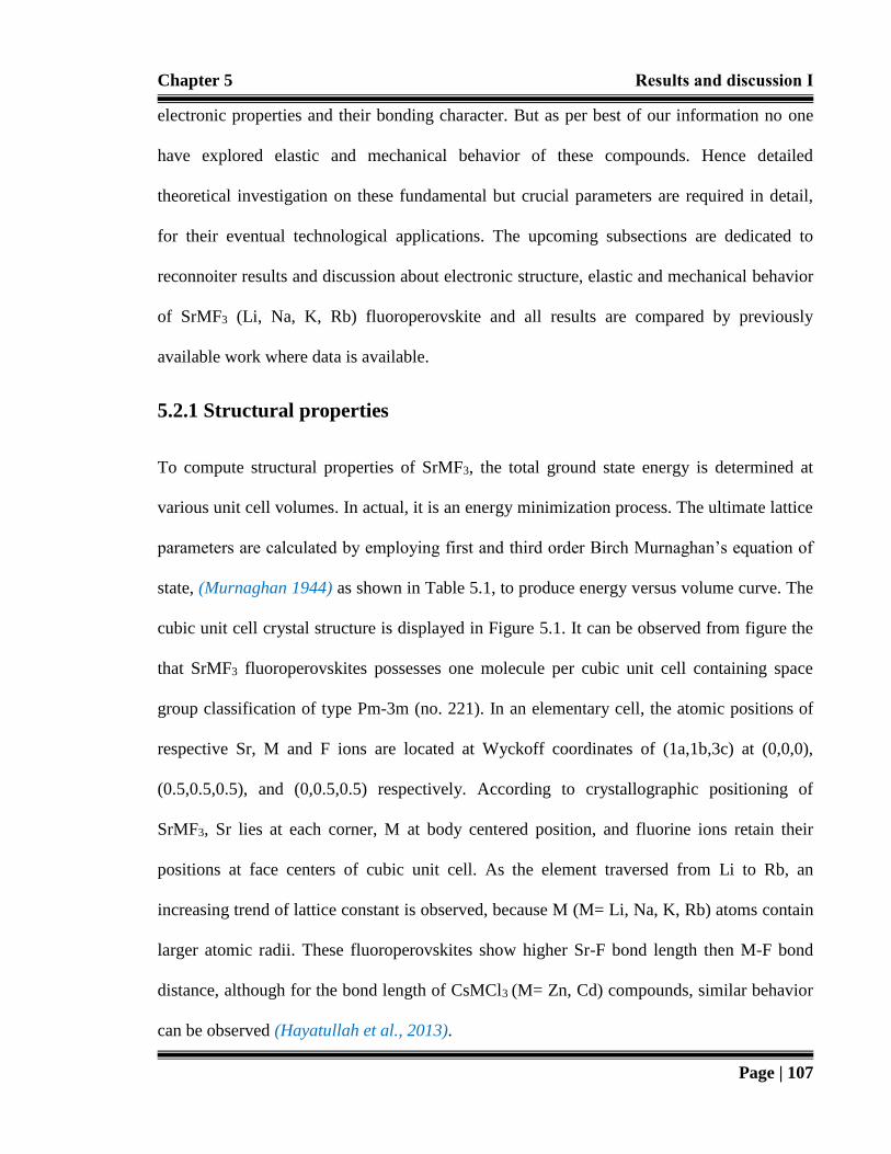
Chapter 5 Results and discussion Ι
Page | 107
electronic properties and their bonding character. But as per best of our information no one
have explored elastic and mechanical behavior of these compounds. Hence detailed
theoretical investigation on these fundamental but crucial parameters are required in detail,
for their eventual technological applications. The upcoming subsections are dedicated to
reconnoiter results and discussion about electronic structure, elastic and mechanical behavior
of SrMF3 (Li, Na, K, Rb) fluoroperovskite and all results are compared by previously
available work where data is available.
5.2.1 Structural properties
To compute structural properties of SrMF3, the total ground state energy is determined at
various unit cell volumes. In actual, it is an energy minimization process. The ultimate lattice
parameters are calculated by employing first and third order Birch Murnaghan’s equation of
state, (Murnaghan 1944) as shown in Table 5.1, to produce energy versus volume curve. The
cubic unit cell crystal structure is displayed in Figure 5.1. It can be observed from figure the
that SrMF3 fluoroperovskites possesses one molecule per cubic unit cell containing space
group classification of type Pm-3m (no. 221). In an elementary cell, the atomic positions of
respective Sr, M and F ions are located at Wyckoff coordinates of (1a,1b,3c) at (0,0,0),
(0.5,0.5,0.5), and (0,0.5,0.5) respectively. According to crystallographic positioning of
SrMF3, Sr lies at each corner, M at body centered position, and fluorine ions retain their
positions at face centers of cubic unit cell. As the element traversed from Li to Rb, an
increasing trend of lattice constant is observed, because M (M= Li, Na, K, Rb) atoms contain
larger atomic radii. These fluoroperovskites show higher Sr-F bond length then M-F bond
distance, although for the bond length of CsMCl3 (M= Zn, Cd) compounds, similar behavior
can be observed (Hayatullah et al., 2013).

Chapter 5 Results and discussion Ι
Page | 108
The analytical calculations of lattice constants are also performed in this work by using two
famous methods. The first method employed ionic radii of the constituent atoms to calculate
lattice constant values. This ionic radius method uses following formula (Clementi et al.,
1963):
𝑎0 = 𝛼 + 𝛽 (𝑟𝑆𝑟 + 𝑟𝐹) + Ɣ(𝑟𝑀 + 𝑟𝐹) (5.1)
The α, β and γ constants in above equation have values of 0.0674, 0.4905 and 1.2921
respectively. And the values for ionic radii are rSr = 1.44 Å, rLi = 1.61 Å, rNa = 1.39 Å, rK =
1.64 Å, rRb = 1.72 Å, rF = 1.285 Å respectively (Erum and Iqbal 2016). The second method
proposed by Verma and Jindal depends on average ionic radii rav, valence electrons number
in Sr, M, and F and some cubic constants, like K (2.45) and S (0.09). The subsequent relation
is as follows (Verma et al., 2008):
𝑎0 = 𝐾(𝑉𝑆𝑟𝑉𝑀𝑉𝐹)𝑠𝑟𝑎𝑣 (5.2)
It can be noticed from Table 5.1 that DFT and analytical calculation of lattice constants
reveal some deviation within 3-4%. This deviation is due to several reasons: Firstly, the
empirical relation for calculating lattice constant by V.J method depends on average ionic
radii. Secondly, the empirical relation for calculating lattice constant by V.J method depends
on number of valence electrons of each atom and thirdly, the error might be due to constants
K (2.45) and S (0.09) which are involved in this empirical relation. Therefore, it can be
concluded that empirical relation given by V.J method needs a lot of improvement to attain
lattice constant values near to experimental one.
To evaluate bonding nature, an important parameter is bond length which depicts an average
distance in between the center point of two bonded atoms because chemical bonding helps to


Chapter 5 Results and discussion Ι
Page | 110
traditional mechanical and cubic stability condition at P = 0 GPa, which can be mentioned by
the following relation C11- C12 > 0, C11 > 0, C44 > 0, C11 + 2C12 > 0 (mechanical stability
condition), and C12 < B < C11 (cubic stability condition). In general, these relations indicate
mechanical stability criteria and cubic stability criteria respectively. Table 5.3 reveals
proportion for elasticity in length C11 is highest for lithium based fluoroperovskite SrLiF3
while it is lowest for rubidium based fluoroperovskite SrRbF3. Meziani and Belkhir (Meziani
and Belkhir 2012) observed the similar results for unidirectional compression along the
principle crystallographic direction. The elasticity in shape can be well explored by elastic
constant of C44. Hence the present calculations reveal that SrMF3 retains more resistance for
shear deformation C44 in comparison with unidirectional compression C11 because the value
of C11 is 605.98%, 486.13%, 649.22%, 306.87%, than C44 for SrRbF3, SrKF3, SrNaF3, SrLiF3
correspondingly.
5.2.3 Mechanical behavior
Many real world versatile mechanical parameters can be evaluated by using elastic constants.
The thermo-elastic stress and strain (internal) are renowned industrial applications of
mechanical properties. The mechanical properties are calculated by GGA approximations as
shown in Table 5.4 and 5.5 respectively.
5.2.3.1 Elastic moduli calculations
The standard description of bulk and shear modulus can be best described by Voigt-Reuss-
Hill (VRH) method (Reuss and Angew 1929). The measure of resistance to reversible
deformation can be best explained by shear modulus G, from following relation (Shafiq et
al., 2011):

Chapter 5 Results and discussion Ι
Page | 111
𝑮𝑽 = 𝟏
𝟓(𝑪𝟏𝟏 − 𝑪𝟏𝟐 + 𝟑𝑪𝟒𝟒) (5.3)
𝑮𝑹 =𝟓𝑪𝟒𝟒(𝑪𝟏𝟏−𝑪𝟏𝟐)
𝟒𝑪𝟒𝟒+𝟑(𝑪𝟏𝟏−𝑪𝟏𝟐) (5.4)
𝑮 =𝑮𝑽+𝑮𝑹
𝟐 (5.5)
However, expression of bulk modulus B are mention from following equation (Kittel 2005):
𝑩 =𝟏
𝟑 (𝑪𝟏𝟏 + 𝟐𝑪𝟏𝟐) (5.6)
It can be observed from Table 5.4 that SrLiF3 has largest value (74.48 GPa, 52.41GPa),
SrRbF3 contains lowest value (33.05GPa, 21.55GPa), of the bulk as well as shear modulus
respectively. In conclusion, SrLiF3 is the hardest material and rest of the compounds are less
harder as compared to SrLiF3 fluoroperovsktie. The response of a material towards linear
strain can be well defined by young’s modulus Y via following relation (Jenkins & Khanna
2005):
𝒚 =𝟗𝑩𝑮
(𝟑𝑩+𝑮) (5.7)
The highest value of B, Y, and G for SrLiF3, implies that there is more tendency of charge
transfer in SrLiF3, rather than SrRbF3, SrKF3 and SrNaF3 respectively. Another significant
ratio which is related to resistance for plastic deformation namely Pugh’s index of ductility or
B/G ratio. For B/G < 1.75 and B/G >1.75 distinguishes compound as brittle or ductile
respectively (Pugh 1954). The SrMF3 series of compounds reveals slightly brittle character
because they satisfied former criteria of Pugh’s index of ductility.
5.2.3.2 Cauchy’s pressure and shear constant calculations
Another important parameter which used to describe angular character in atomic bonding is
Cauchy’s pressure. It can be well defined as follows (Brik 2011):

Chapter 5 Results and discussion Ι
Page | 112
𝑪′′ = 𝑪𝟏𝟐 − 𝑪𝟒𝟒 (5.8)
Negative values of Cauchy’s pressure (𝐶′′) indicate high angular characteristics in bonding
while compound with positive Cauchy’s pressure tend to form metallic bond in nature. For
B/G less than 1.75 and Cauchy’s pressure less than zero implies that SrMF3 compounds are
not ductile in nature and retain less tendency of covalent bonding. As a result, compounds
have dominant ionic behavior. To further distinguish between, ionic or covalent behavior the
present analysis is extended to evaluate shear constant. However low values of shear
constants depict ionic behavior and vice versa. It can be expressed as:
𝑪′ =𝟏
𝟐(𝑪𝟏𝟏 − 𝑪𝟏𝟐) (5.9)
From Table 5.5 it is evident that SrMF3 have low values of shear constant so tend towards
ionic in behavior.
5.2.3.3 Poisson’s ratio and elastic anisotropy calculations
Next, ratio of compression to relative expansion can be expressed in terms of Poisson’s ratio,
as follows (Pettifor 1992):
ѵ =(𝟑𝑩−𝟐𝑮)
𝟐(𝟑𝑩+𝑮) (5.10)
As per Gu and his fellows (Gu et al., 2014) for central force solids respective upper and
lower limits are 0.25 and 0.5. In another investigation Haines with his co-researchers (Haines
et al., 2001) suggested that for ionic material it is less than 0.1. Hence it can be clearly
demonstrated from Table 5.5 that SrMF3 compounds resist more for ionic character and least
partial covalent character and from several mechanical parameters it can be well concluded
that SrLiF3 show more brittle behavior than rest of the compound.
In manufacturing disciplines, elastic anisotropy parameter (A) plays an imperative character.
The relation can be well defined as follows (Jamal et al., 2016):

Chapter 5 Results and discussion Ι
Page | 113
𝑨 =𝟐𝑪𝟒𝟒
(𝑪𝟏𝟏−𝑪𝟏𝟐) (5.11)
If A is equal to unity, then the crystal can be completely characterized as isotropic. However,
when micro-cracks are introduced within the material than the value of A, deviates from
unity and the degree of deviation measures amount of elastic anisotropy. However, value of
A of SrMF3 is less than unity that clearly shows anisotropic behavior of corresponding
materials. In fact, anisotropy decreases on addition of the cation with less atomic size and
vice versa.
5.2.3.4 Melting temperature Tm and Kleinman’s parameter calculations
To calculate melting tendency of SrMF3 compounds, the next task is to explore melting
temperature, above which material changes from its solid phase to its liquid phase (Fine et
al., 1984):
Tm = 607 + 9.3B + 555 (5.12)
The GGA calculation of melting temperature are basically consistent with aforementioned
behavior of the compounds. The pictorial representation of melting temperature from Figure
5.3 shows that melting temperature increases as compounds traverses from SrRbF3 to SrLiF3
respectively. Another significant parameter which was introduced by Kleinman, used to
quantify material’s behavior towards bond stretching or bond bending; if minimum bond
stretching then Kleinman parameter (ξ), ξ=1 but If compound possess minutest value for
bond bending then ξ=0 (Kleinman 1962), as:
𝝃 =𝑪𝟏𝟏+𝟖𝑪𝟏𝟐
𝟕𝑪𝟏𝟏−𝟐𝑪𝟏𝟐 (5.13)
The range of value lie between 0.22-0.42 as compound changes from SrRbF3 to SrLiF3 which
shows that in SrRbF3 bond bending is prevalent while bond stretching is dominant in SrLiF3
fluoroperovskite.

Chapter 5 Results and discussion Ι
Page | 114
5.2.3.5 Lame’s constant calculations
At the end, the study is related with stress to strain by acknowledging two important
constants namely first λ and second μ Lame’s constant. The expression for these constants
can be derived from various mechanical parameters in the following form (Alouani 1991):
𝝀 = 𝒀ѵ
(𝟏+ѵ)(𝟏−𝟐ѵ) (5.14)
𝝁 =𝒀
𝟐(𝟏+ѵ) (5.15)
Above equations reveals that these constants are in direct relation with the value of Y. Our
calculated values not fulfill the specific criteria 𝜆 = 𝐶12 𝑎𝑛𝑑 𝜇 = 𝐶′ for isotropic material.
So SrMF3 is a class of anisotropic compounds which is in accordance with the calculated
value of anisotropy parameters. In conclusion, an increase in anisotropy is observed in the
following fashion SrLiF3→ SrNaF3→ SrKF3→ SrRbF3. Hence these compounds can be used
in manufacturing low birefringence lens materials. As a result, through this study various
quantum mechanical effects have benchmarked which are very beneficial to utilize and
understand in manufacturing practical devices.
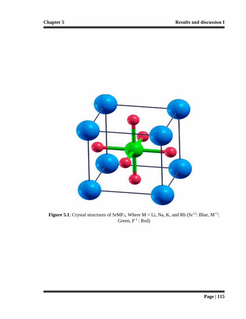
Chapter 5 Results and discussion Ι
Page | 115
Figure 5.1: Crystal structures of SrMF3, Where M = Li, Na, K, and Rb (Sr+2: Blue, M+1:
Green, F-1 : Red)

Chapter 5 Results and discussion Ι
Page | 116
Figure 5.2: Lattice constants versus change in bond lengths between M and F of SrMF3
(M = Li, Na, K, Rb).
Figure 5.3: Melting temperature Tm (K) Vs Klienmann parameter ξ (GPa).
SrLiF3
SrNaF3
SrKF3
SrRbF3
3.13
3.14
3.15
3.16
3.17
3.18
3.19
3.2
3.21
3.22
4 4.2 4.4 4.6 4.8 5
Bo
nd
-len
gth
s M
-F (
Å)
Lattice constant (Å)
SrLiF3SrNaF3
SrKF3 SrRbF3
0
500
1,000
1,500
2,000
2,500
3,000
0.42 0.23 0.24 0.22
Tm
(K)
ξ(GPa)

Chapter 5 Results and discussion Ι
Page | 117
Table 5.1: Comparison of calculated equilibrium lattice constants (ao), ground state energies
(Eo) and bulk modulus (Bo) with experimental and other theoretical values of SrMF3 (X = Li,
Na, K and Rb) compounds.
a (Mousa et al., 2013), b (Mubarak 2014), c (Düvel et al., 2011), d (Yamanoi et al., 2014), e (Ouenzerfi
2004) (Other theoretical work) f (Castro 2002), g (Mishra 2011) (Experimental Work)
Table 5.2: Bond-lengths of SrMF3 (X= Li, Na, K, Rb) compounds.
Compound Present
─────────
GGA
Work
─────────
LDA
─────────
I.R method
─────────
V.J method
Theoretical
work
Experimental
work
SrLiF3
ao (Å)
Eo (Ry)
Bo (GPa)
4.11
-6974.884
73.482
4.08
-6974.901
4.81
4.79
3.88a, b,
3.87c
3.76d, 3.75e
72.87a,71.5b
4.45f
72.07g
SrNaF3
ao (Å)
Eo (Ry)
Bo (GPa
4.23
-7284.587
56.59
4.16
-7284.601
4.71
4.45
4.18a
55.81a
4.44f
SrKF3
ao (Å)
Eo (Ry)
Bo (GPa)
4.43
-8163.855
37.62, 47.52
4.41
-8163.728
4.88
4.71
4.38a
37.69a
4.49f
29.64f
SrRbF3
ao (Å)
Eo (Ry)
Bo (GPa)
4.49
-12922.447
32.24
4.46
-12922.386
4.98
5.01
4.55a
31.62a
4.47f
30.6f
SrLiF3
Bond
length
(Å)
SrNaF3
Bond
length
(Å)
SrKF3
Bond
length
(Å)
SrRbF3
Bond
length
(Å)
Sr-F (Å) 2.52 Sr-F (Å) 2.55 Sr-F (Å) 2.58 Sr-F (Å) 2.60
Li-F (Å) 1.85 Na-F (Å) 2.23 K-F (Å) 2.60 Rb-F (Å) 2.74
Sr-Li (Å) 3.23 Sr-Na (Å) 3.61 Sr-K (Å) 3.98 Sr-Rb (Å) 4.15

Chapter 5 Results and discussion Ι
Page | 118
Table 5.3: Calculated values of elastic constants C11, C12, C44, for SrMF3 (X = Li, Na, K and
Rb) compounds.
Table 5.4: Calculated values of Bulk modulus B0, Voigt’s shear modulus GV, Reuss’s shear
modulus GR, Hill’s shear modulus GH, Young’s modulus Y, and Pugh’s index of ductility
Bo/GH.
Sr.No. Parameters SrLiF3 SrNaF3 SrKF3 SrRbF3
1 C11 (GPa) 151.741 145.490 98.101 85.390
2 C12 (GPa) 37.353 12.140 9.021 6.881
3 C44 (GPa) 49.447 22.410 20.180 14.091
Sr.No. Parameters SrLiF3 SrNaF3 SrKF3 SrRbF3
1 Bo(GPa) 74.481 56.590 38.710 33.051
2 Gv(GPa) 52.541 40.122 29.924 24.156
3 GR(GPa) 52.279 30.511 25.833 18.954
4 GH(GPa) 52.414 35.315 27.872 21.551
5 Y (GPa) 127.361 87.703 67.427 53.107
6 Bo/GH (GPa) 1.421 1.605 1.385 1.532

Chapter 5 Results and discussion Ι
Page | 119
Table 5.5: Calculated values of Shear constant (𝐶′), Cauchy pressure (𝐶′′), Poisson’s ratio
(ѵ), Anisotropy constant (A), Kleinman parameter (ξ), Lame’s coefficients (λ and μ), and
Melting temperature (Tm).
Sr.No. Parameters SrLiF3 SrNaF3 SrKF3 SrRbF3
1 𝐶′ 57.19 66.67 44.54 39.25
2 𝐶′′ -12.09 -10.27 -11.16 -7.21
3 Ѵ (GPa) 0.21 0.24 0.22 0.23
4 A (GPa) 0.86 0.34 0.45 0.36
5 ξ(GPa) 0.42 0.23 0.24 0.22
6 λ 39.53 32.64 20.17 18.56
7 μ 52.40 35.36 27.86 21.58
8 Tm(K) 1854 1688 1522 1469

Chapter 5 Results and discussion Ι
Page | 120
5.3 Opto-electronic investigation of SrMF3 (M = Li, Na, K, Rb)
5.3.1 Electronic properties
The electronic properties of SrLiF3, SrNaF3 SrKF3 SrRbF3 fluoroperovskites are analyzed by
electronic band dispersion curves, detailed states for density while chemical nature of
bonding is interpreted by electron density contour maps.
5.3.1.1 Band structure calculations
Dispersion curves of computed bandgap are displayed in Figure 5.4 - 5.7 respectively. The
bandgap results are taken in first brillouin zone. Here to get reliable results, DFT bandgap is
treated with five distinct exchange and correlation schemes. Detailed theoretical chemistry
for band structure are itemized in Table 5.6. The current calculations from LDA as well as
PBE-GGA approximations are in good agreement with previously available work. Though,
these approximations underestimate the bandgap in semiconductors as well as in insulators
due to wrong interpretation of the true unoccupied states with respect to consistent Khon–
Sham DFT states (Wu and cohen 2006). To acquire nearby experimental values and to
overcome band gap underestimation, we graphically only present results by modified Becke-
Johnson potential (mBJ).
Calculated outcomes depict SrMF3 contains both maxima as well as minima of valence and
conduction bands at (Γ- Γ) symmetry points as a result provides minimum direct band gap
and it can be analyzed from Table 5.6 that bandgap is going to decrease from SrLiF3 to
SrRbF3 and vice versa because minima of conduction band move closer to Fermi level (EF).
The similar results for direct (Γ-Γ) gap are also observed for BaLiF3, CaLiF3 and CsSrF3
(Mousa et al., 2013 & babu et al., 2012) however different behavior is observed for RbCdF3,

Chapter 5 Results and discussion Ι
Page | 121
RbZnF3, as well as RbHgF3 (Murtaza et al., 2013) having indirect bandgap at (M-Γ) which
depicts that nature of electronic properties for fluoroperovskites varies as of compound to
compound. Additionally, through mBJ potential a bandgap near to experimental values is
obtained like Yalcin and their fellows (Yalcin et al., 2016), calculated 8.2 eV bandgap for
mBJ potential, alike to BaLiF3 experimental bandgap of 8.41 eV. Consequently, just 1.78%
deviation has been observed. Analogous findings are observed for SrMF3 compounds.
5.3.1.2 Density of States (DOS) calculations
The investigated outcomes of density of states (DOS) indicate wide dispersion of electronic
bands as shown in Figure 5.8 (DOS for SrLiF3), Figure 5.9 (DOS for SrNaF3), Figure 5.10
(DOS for SrKF3), and Figure 5.11 (DOS for SrRbF3) respectively. In conduction band Sr-3d
peaks appears nearby 5.9, 6.6, 8.8, 9.2 eV for SrRbF3, SrKF3, SrNaF3, SrLiF3 correspondingly.
Though, SrRbF3 and SrKF3 shows crossed crests of Rb-3d and K-3d within range of 5-10 eV.
The valence band resides within energy range as of 0 to -30 eV. The evolution of fluorine 2p
governs valence band region till -2.5 eV, together with little influence of Sr and M states.
Likewise, hybridized crests are observed in -20 to -23 eV for F-2s as well as M states
respectively. Furthermore, triplet degenerate energy levels at Γ symmetry point are observed
for lower conduction and upper valence gap regions. At -13.8 and -15.1 eV, peaks in SrLiF3
and SrNaF3 are due to Sr-4p states individually. In valence band region, for SrKF3 and
SrRbF3, K-3p and Rb-4p states are observed at -8.5 eV and -6.5 eV. In SrMF3 different peaks
at different energy levels are appeared for example, Na-2p state at -17.2 eV, K-4s states at -
25.8 eV, Rb-5s state at -22.6 eV for SrNaF3, SrKF3, SrRbF3 respectively.

Chapter 5 Results and discussion Ι
Page | 122
5.3.1.3 Electron density contour calculations
In crystalline solids nature of chemical bonding, can be determined via electron density,
contour maps (Hoffman 1988). Electron density distribution curves are presented in 2D and
3D, along (100) and (110) planes. It can be observed from Figure 5.12 (a-d) that, in (100)
plane dispersal of charge for SrLiF3 is not clearly spherical within Sr and F cation as well as
anion respectively. However, it is perfectly spherical for SrRbF3, SrNaF3, and SrKF3 that is
due to predominant ionic bonding nature. Whereas as of view from (110) plane, as shown in
Figure 5.13 (a-d) and 5.14, it can be analyzed that, charge is transferred between M cation as
well as F anion because of huge electronegativity variance where transference of charge in
octahedral differs as per subsequent relation: LiF6 > NaF6 > KF6 > RbF6 in addition to it,
nature of covalent bonding corresponds accordingly: SrRbF3 > SrKF3 > SrNaF3 > SrLiF3. In
fact, atomic magnitude becomes larger when moving down in a group and corresponding
electrons in bigger atoms are not capable to stay strongly in comparison with smaller ones
which reduces extent of electronegativity. Hence increase in ionic behavior can be observed
as compound moves from SrLiF3 to SrRbF3 While this investigation matches well by
consequences of DOS where maximum p-d hybridization is obtained in SrLiF3. Furthermore,
parallel trend of outcomes was also observed in the work done by Harmel and their co-
fellows (Harmel et al., 2015 & Harmel et al., 2012).
5.3.2 Optical parameters
In order to calculate fundamental and derived optical responses of SrMF3, exchange
correlation potential of modified Becke–Johnson (mBJ) with GGA is applied. The details of
evaluated parameters are mentioned in few upcoming headings.
Chapter 5 Results and discussion Ι
Page | 123
5.3.2.1 Complex dielectric constant calculations
The Ԑ(ω) can be defined as follows (Fox 2001):
Ԑ(𝜔) = Ԑ1(𝜔) + 𝑖Ԑ2(𝜔) (5.16)
In equation 5.16 Ԑ(ω), Ԑ1(ω) and Ԑ2(ω) represents complex, real as well as imaginary
dielectric function respectively. Generally, Ԑ1(ω) can influences in two ways such as
intraband as well as interband transitions. For metals, the contribution of intraband transition
is exclusively significant. While further classification of interband transitions can be done in
terms of indirect and direct transitions (Dressel 2001). However, the present calculations are
performed by considering results of direct (interband) transitions. Ԑ2(ω) can be given as:
Ԑ2(𝜔) = (4𝜋2𝑒2
𝑚2𝜔2) ∑ ∫ ⟨𝑖|𝑀|𝑗⟩2𝑓𝑖(1 − 𝑓𝑖)𝛿(𝐸ј,𝑘 − 𝐸𝑖,𝑘 − 𝜔)𝑘𝑖,𝑗 𝑑3𝑘 (5.17)
In equation 5.17 initial and final states are denoted by ὶ and ј respectively, the dipole matrix
is represented by M, ω is the resonance frequency. In spectra of Ԑ2(ω), as shown in Figure
5.15 (a) wide-ranging characteristic peaks are observed which can be directly linked to DOS
of the respective compounds for further clarification. First critical point or threshold energy
for SrLiF3, SrNaF3, SrKF3 and SrRbF3 are occurred approximately at 9.3 eV, 8.9 eV, 7.2 eV
and 5.8 eV respectively. For direct optical transitions, this threshold energy gives
corresponding fundamental gap at equilibrium, which is also recognized as fundamental
absorption edge. It ensues due to splitting between highest states of valence band at (Γv) to
lowest state of conduction band at (Γc). In fact, the materials with band gaps greater than 3.1
eV can work well in the Ultra-Violet region so all compounds can work well in ultraviolet
region of electromagnetic spectrum (Wooten 1972). It can be observed that fundamental

Chapter 5 Results and discussion Ι
Page | 124
absorption edge shift towards lower energy as we move towards Li to Rb. After the incent of
critical point, Ԑ2(ω) dispersion curves increases abruptly due to rapid contribution of
electronic states. As a result, the principle peak is situated at 12.2 eV for SrLiF3, 10.9 eV for
SrNaF3, 8.3 eV for SrKF3 and 6.9 eV SrRbF3, correspondingly which is in accordance with
the trends of DOS and band-structure. These peaks are attributed to transitions of F-2p state
alongwith minor influences of Sr-3d and M-states positioned just below zero energy Fermi
level (EF). However, using the knowledge of optical matrix element SrKF3 and SrRbF3
compounds reveals hybridized peaks around 5 to 10 eV of K-3d and Rb-3d respectively. The
real part of dielectric function Ԑ1(ω) is given by the well-known Kramers-Kronig relation via
corresponding equation (Erum and Iqbal, November 2017):
Ԑ1(𝜔) = 1 +2
𝜋𝑃 ∫
ὠԐ2(ὠ)𝑑ὠ
ὠ2−ὠ2
ⱷ
0 (5.18)
It describes Ԑ1(ω) defines electric polarizability and absorptive behavior of the material. The
dielectric function (static part), as shown in Figure 5.15 (b), Ԑ1(0) at zero frequency limit is
calculated at about 1.61 eV to 1.71 eV for SrMF3 compounds, correspondingly. Similar trend
of static refractive index is observed. The curves of Ԑ1(ω) starts increasing from the (zero)
limit of frequency and attains maxima value to expose the principle peak which is at about
6.6 eV, 7.9 eV, 9.5 eV and 10.3 eV for SrRbF3, SrKF3, SrNaF3 and SrLiF3, exclusively.
5.3.2.2 Optical conductivity and energy loss calculations
The calculated values of complex dielectric function Ԑ(ω) can allow to determine key optical
function for the electromagnetic spectrum such as optical conductivity σ(ω), and electron
energy loss spectrum L(ω) which can be determined by following expressions (Fox 2001):

Chapter 5 Results and discussion Ι
Page | 125
𝐿(𝜔) = 𝐼𝑚 (−1
Ԑ(𝜔)) (5.19)
𝜎(𝜔) = 2𝑊𝐶𝑉ℏ𝜔
𝐸02 (5.20)
In equation 5.20 WCV is the transition probability between conduction and valence band. The
calculated spectrum of L(ω) is figured in Figure 5.15(c). It relates microscopic as well as
macroscopic responses of material and elucidates characteristic contribution associated with
plasma resonance frequency (ωp) (Waghmare 2001). The peaks in L (w) spectra narrate
energy loss of electron that is traversing rapidly within the material. The region of distinct
sharp peak covers range within 7 eV to 14 eV for M compounds respectively. The calculated
optical conductivity σ(ω) for SrMF3 fluoroperovskites are shown in Figure 5.15(d). The drift
of figure reveals that the phenomenon of σ(ω) optical conductivity begins at approximately 4
eV. The journey of optical conductivity traverses from small and large peaks and finally
reveals steady behavior in high-energy ranges. It is evident from above analysis that from
cation Rb to Li, the spectrum of σ(ω) shift towards low energy ranges.
5.3.2.3 Sum rules calculation via neff
In the end, the sum rule is evaluated to consider the number of effective valence electrons via
corresponding formula (Abelès 1972):
𝑛𝑒𝑓𝑓(𝜔) = ∫ 𝜎(ὠ)𝜔
0ὠ 𝑑ὠ (5.21)
From Figure 5.15 (e) trends of sum rule can be analyzed, which originates the inter-band
transition of electrons at about 5.5 eV. Then there is slow increase in trendline, however
advent of (sharp) peak reveals abrupt increment of electron which saturates in the range at

Chapter 5 Results and discussion Ι
Page | 126
about 14-16 eV and onwards. The results of neff are in similar accordance with the above
calculated optical parameters.
Figure 5.4: The mBJ-electronic band dispersion curves for SrLiF3
En
ergy
(eV
)

Chapter 5 Results and discussion Ι
Page | 127
En
erg
y (
eV)
Figure 5.5: The mBJ-electronic band dispersion curves for SrNaF3

Chapter 5 Results and discussion Ι
Page | 128
En
ergy
(eV
)
Figure 5.6: The mBJ-electronic band dispersion curves for SrKF3

Chapter 5 Results and discussion Ι
Page | 129
Figure 5.7: The mBJ-electronic band dispersion curves for SrRbF3
En
ergy
(eV
)

Chapter 5 Results and discussion Ι
Page | 130
Figure 5.8: The Density of States for SrLiF3 by mBJ potential
Energy (eV)
DO
S (
Sta
tes/e
V)

Chapter 5 Results and discussion Ι
Page | 131
Energy (eV)
DO
S (
Sta
tes/e
V)
Figure 5.9: The Density of States for SrNaF3 by mBJ potential

Chapter 5 Results and discussion Ι
Page | 132
Energy (eV)
DO
S (
Sta
tes/e
V)
Figure 5.10: The Density of States for SrKF3 by mBJ potential

Chapter 5 Results and discussion Ι
Page | 133
DO
S (
Sta
tes/e
V)
Energy (eV)
Figure 5.11: The Density of States for SrRbF3 by mBJ potential

Chapter 5 Results and discussion Ι
Page | 134
Figure 5.12 (a): Calculated mBJ total two and three-dimensional electronic charge densities
for SrLiF3 in (100) plane.

Chapter 5 Results and discussion Ι
Page | 135
Figure 5.12 (b): Calculated mBJ total two and three-dimensional electronic charge densities
for SrNaF3 in (100) plane.

Chapter 5 Results and discussion Ι
Page | 136
Figure 5.12 (c): Calculated mBJ total two and three-dimensional electronic charge densities
for SrKF3 in (100) plane.

Chapter 5 Results and discussion Ι
Page | 137
Figure 5.12 (d): Calculated mBJ total two and three-dimensional electronic charge densities
for SrRbF3 in (100) plane.

Chapter 5 Results and discussion Ι
Page | 138
Figure 5.13 (a): Calculated mBJ total two and three-dimensional electronic charge densities
for SrLiF3 in (110) plane.

Chapter 5 Results and discussion Ι
Page | 139
Figure 5.13 (b): Calculated mBJ total two and three-dimensional electronic charge densities
for SrNaF3 in (110) plane.

Chapter 5 Results and discussion Ι
Page | 140
Figure 5.13 (c): Calculated mBJ total two and three-dimensional electronic charge densities
for SrKF3 in (110) plane.

Chapter 5 Results and discussion Ι
Page | 141
Figure 5.13 (d): Calculated mBJ total two and three-dimensional electronic charge densities
for SrRbF3 in (110) plane.

Chapter 5 Results and discussion Ι
Page | 142
Figure 5.14: Total two-dimensional electron density plots in (110) plane for (a) SrLiF3, (b)
SrNaF3, (c) SrKF3, (d) SrRbF3.

Chapter 5 Results and discussion Ι
Page | 143
Figure 5.15 (a): Calculated imaginary part Ԑ2 (ω) of the dielectric function for the SrMF3
(M=Li, Na, K, Rb) compounds.

Chapter 5 Results and discussion Ι
Page | 144
Figure 5.15 (b): Calculated real part Ԑ1(ω) of the dielectric function for the SrMF3
(M=Li, Na, K, Rb) compounds.
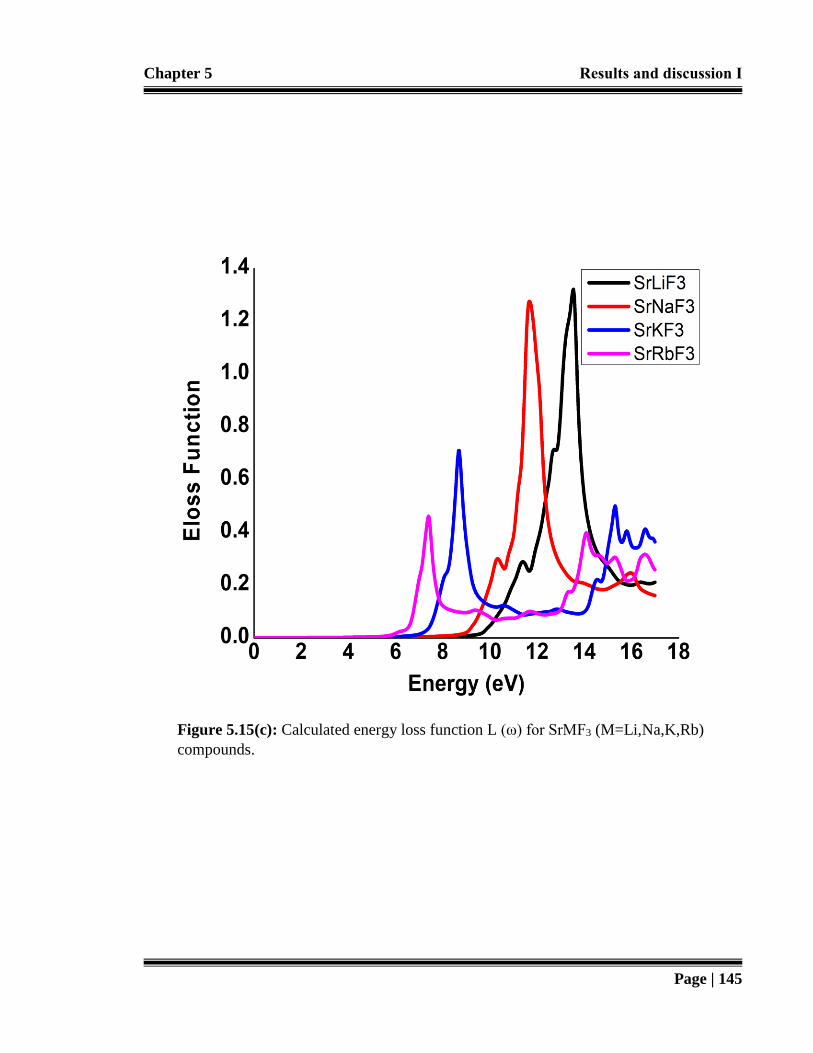
Chapter 5 Results and discussion Ι
Page | 145
Figure 5.15(c): Calculated energy loss function L (ω) for SrMF3 (M=Li,Na,K,Rb)
compounds.

Chapter 5 Results and discussion Ι
Page | 146
Figure 5.15(d): Calculated conductivity σ(ω) for SrMF3 (M= Li, Na, K, Rb) compounds.

Chapter 5 Results and discussion Ι
Page | 147
4.3. Opto-electronic investigation of Rubidium based Fluoro-Perovskite for
. Figure 5.15(e): Calculated sum rule for SrMF3 (Li,Na,K,Rb) compounds.
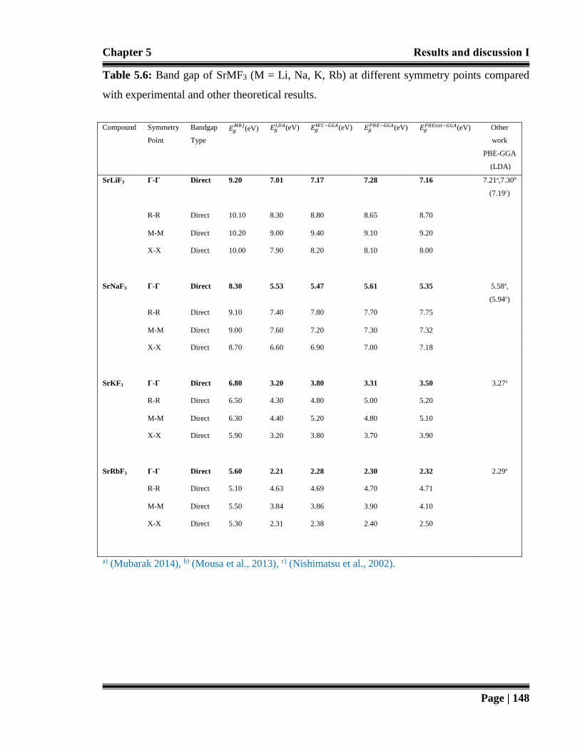
Chapter 5 Results and discussion Ι
Page | 148
Table 5.6: Band gap of SrMF3 (M = Li, Na, K, Rb) at different symmetry points compared
with experimental and other theoretical results.
Compound Symmetry
Point
Bandgap
Type
𝐸𝑔𝑀𝐵𝐽
(eV) 𝐸𝑔𝐿𝐷𝐴(eV) 𝐸𝑔
𝑊𝐶−𝐺𝐺𝐴(eV) 𝐸𝑔𝑃𝐵𝐸−𝐺𝐺𝐴(eV) 𝐸𝑔
𝑃𝐵𝐸𝑠𝑜𝑙−𝐺𝐺𝐴(eV) Other
work
PBE-GGA
(LDA)
SrLiF3 Γ-Γ Direct 9.20 7.01 7.17 7.28 7.16 7.21a,7.30b
(7.19c)
R-R Direct 10.10 8.30 8.80 8.65 8.70
M-M Direct 10.20 9.00 9.40 9.10 9.20
X-X Direct 10.00 7.90 8.20 8.10 8.00
SrNaF3 Γ-Γ Direct 8.30 5.53 5.47 5.61 5.35 5.58a,
(5.94c)
R-R Direct 9.10 7.40 7.80 7.70 7.75
M-M Direct 9.00 7.60 7.20 7.30 7.32
X-X Direct 8.70 6.60 6.90 7.00 7.18
SrKF3 Γ-Γ Direct 6.80 3.20 3.80 3.31 3.50 3.27a
R-R Direct 6.50 4.30 4.80 5.00 5.20
M-M Direct 6.30 4.40 5.20 4.80 5.10
X-X Direct 5.90 3.20 3.80 3.70 3.90
SrRbF3 Γ-Γ Direct 5.60 2.21 2.28 2.30 2.32 2.29a
R-R Direct 5.10 4.63 4.69 4.70 4.71
M-M Direct 5.50 3.84 3.86 3.90 4.10
X-X Direct 5.30 2.31 2.38 2.40 2.50
a) (Mubarak 2014), b) (Mousa et al., 2013), c) (Nishimatsu et al., 2002).

Chapter 5 Results and discussion Ι
Page | 149
5.4 Opto-electronic investigation of RbHgF3 for low birefringent
lens materials
Physical properties of material have played principle role in implementation of them in
specific area of device fabrication. To fulfill this curiosity material scientists are vigilant to
inquire opto-electronic response of different perovskite compounds. Now-a-days rubidium
series of mercury fluoroperovskite is renowned to own several technological benefits. One of
the important application of RbHgF3 is in fabricating lens materials with low birefringence
because high birefringence can make design of lenses difficult. Further it conceives wide
range of opto-electronic and photonic applications such as in optical pathways, UV detectors,
transparent optical coatings and Light Emitting diodes (LED) (Lang et al., 2014 &
Vaitheeswaran et al., 2007).
5.4.1 Structural properties
In order to investigate ground state structural aspects of RbHgF3, the total energy is
determined at various volumes. The structural properties are calculated by using energy
minimization process as described in section 5.1.1 in detail. It can be observed from Figure
5.16 that RbHgF3 fluoroperovskite compound crystallized it-self in cubic structure while sites
of Wyckoff coordinates are situated at 1a, 1b, and 3c for respective cations and anions of Rb,
Hg and F. These structural findings are in similar accordance with comprehensive
experimental investigation done by Dotzler and their fellows (Dotzler et al., 2008).
The variation of total energy as a function of unit cell volume is displayed in Figure 5.17 and
calculated lattice parameters such as ground state energy (Eo), equilibrium lattice constant
(ao), bulk modulus (Bo) and its pressure derivative (Bp) are tabulated in Table 5.5 with four

Chapter 5 Results and discussion Ι
Page | 150
different schemes (LDA, PbE-GGA, WC-GGA and PBEsol-GGA). The slightly overvalued
DFT calculated lattice constant as compared to experimental one can be attributed to the use
of traditional DFT approximations. Furthermore, good crystal rigidity is evident from the
value of bulk modulus but on the other hand, a contrary relation between value of bulk
modulus and lattice constant can be observed from Table 5.5, in similar accordance with the
pattern of another halide perovskite (Ghebouli et al., 2012; Brik 2011& Rose et al., 1993).
5.4.2 Electronic Properties
In this section, calculations of electronic behavior of RbHgF3 have been done in terms of
band structure, Density of states (DOS), (Total as well as Partial) and nature of bonding is
explained in terms of electron density plots.
5.4.2.1 Band structure calculations
In this study the computation of bandgap is done with the help of GGA plus Tran-Blaha
modified Becke–Johnson (TB-mBJ) potential (Tran and Blaha 2009). The comparison of
energy band structures at high symmetry direction from PBE-GGA and mBJ schemes are
shown in Figure 5.18, which proves bandgap underestimation by PBE-GGA approximation.
It can be noted that trend of overall dispersion in a band structure curves are almost same and
lower edge of conduction and higher edge of valence band lies at M and Γ symmetry points
along the Brillouin Zone (BZ), resulting an indirect (M-Γ) bandgap of about 0.7 eV from
PBE-GGA and 3.1 eV from mBJ schemes respectively. However, in order to make a
reasonable comparison, there is lack of experimental data of bandgap. An important
application of this material is in Ultra-Violet region of electromagnetic spectrum because it

Chapter 5 Results and discussion Ι
Page | 151
has bandgap larger than 3.1 eV so work efficiently for UV-based practical devices (Lang
2014).
5.4.2.2 Density of States (DOS) calculations
The detailed analysis of partial and total density of states are done by analyzing various states
of corresponding energy density distribution, as shown in Figure 5.19. The significant peaks
of DOS are found within -10 to15 eV. At -10 eV, a fine peak can be notified because of Rb-
4p states. Next, in valence band region from fermi-level to -6.1 eV an overlapping is
observed between F-2p and Hg-3d states and above the fermi level, the upper and lower part
of conduction band is filled by Hg-4s as well as Rb-4d states respectively.
5.4.2.3 Electron density contour calculations
In crystalline materials, nature of chemical bonding can be communicated via map of
electron density plots (Gelatt 1983). The 2D and 3D contour maps along (100) and (110)
planes are shown in Figure 5.20 (a, b) and 5.21 (a, b) respectively. In contour maps of Rb
cation and F- anion due to large electronegativity difference, transfer of charge occurred.
However, the perfectly spherical charge distribution confirms strong ionic character in Rb-F
bond. Furthermore, uniform distribution of charge between Hg cation and F anion validates
covalent character of HgF3 type octahedra. The bonding nature by these plots are in exact
accordance with the plots of Density of states as shown in Figure 5.19, where in between Hg-
3d and F-2p states, the p-d hybridization is maximum. Hence confirms mixed covalent and
ionic bonding character in rubidium based fluoroperovskite. In a similar study, Harmel and
their fellows (Harmel et al., 2015) observed the same results for cesium based
fluoroperovskites.

Chapter 5 Results and discussion Ι
Page | 152
5.4.3 Optical properties
The tool of optical analysis is employed to expose internal behavior of RbHgF3 compound.
Imaginary and real part of dielectric function are two fundamental optical responses.
However, in concern with, practical device applications analysis is extended to plot spectra
of reflectivity and optical absorption.
5.4.3.1 Complex dielectric constant calculations
The complex dielectric function consists of two parts, namely imaginary and real part (Fox
2001):
Ԑ(𝜔) = Ԑ1(𝜔) + 𝑖Ԑ2(𝜔) (5.22)
Imaginary part of dielectric function can be denoted in terms of Ԑ2(ω) while Ԑ1(ω) depicts
about real part of dielectric function. The comprehensive response of a material due to
applied electromagnetic radiation in terms of Ԑ2(ω) are shown in Figure 5.22(a). In this
optical study focus is paid to direct interband transition while taking into account appropriate
element of transition dipole matrix (Brik 2011). The band structure and DOS of the
investigated compound follow the pattern of widespread peaks of Ԑ2(ω). The major peak in
Ԑ2(ω) are located at approximately 22.1 eV and threshold energy point occurs at 4.4 eV
approximately. The occurrence of these diversified peaks are observed due to hybridized
states of Rb-4d with some p states of mercury and fluorine. The real part of dielectric
function Ԑ1(ω) depicts the absorptive behavior as figured out in Figure 5.22(b). The dielectric
function, static part is notified at 1.88 eV. The ascending peaks in Ԑ1(ω) attains maximum

Chapter 5 Results and discussion Ι
Page | 153
position around 6 eV, which confirms an overall narrow bandgap semi-conductive nature,
while minimum attains at 20 eV.
5.4.3.2 Absorption coefficient calculations
The absorption of electromagnetic radiation in optical absorption spectra of RbHgF3 starts at
about 5.05 eV as shown in Figure 5.22 (c). This particular energy point is in exact
accordance with the trend of bandgap. After some ascending peaks, RbHgF3 starts absorbing
effectively, delivers prominent peaks at around 21.5 eV. After trivial variations, the peaks
again going to decrease. The absorption spectra analysis concludes application of RbHgF3 for
wide absorption purposes at about 21.5 eV in Ultra-Violet region of electromagnetic
spectrum.
5.4.3.3 Optical reflectivity calculations
Figure 5.22 (d), depicts phenomenon of reflectivity as a function of energy. It can be
observed that up to 19 eV the phenomenon of reflectivity stays below 9-10%. However, at 22
eV material attains high value of reflectivity in high energy region. As a result, it can be
concluded that RbHgF3 is one of the prospective material for efficient lenses as well as
transparent coating devices because in infrared (IR) as well as visible regions these materials
remain highly transparent.

Chapter 5 Results and discussion Ι
Page | 154
Figure 5.16: Cubic crystal structure of RbHgF3

Chapter 5 Results and discussion Ι
Page | 155
Figure 5.17: Variation of total energy as a function of unit cell volume for RbHgF3

Chapter 5 Results and discussion Ι
Page | 156
Figure 5.18: Comparison of band structures in high symmetry directions with mBJ and
PBE-GGA schemes for RbHgF3
En
erg
y (
eV
)

Chapter 5 Results and discussion Ι
Page | 157
Energy (eV)
DO
S (
Sta
tes/e
V)
Figure 5.19: The Density of States for RbHgF3 by mBJ potential

Chapter 5 Results and discussion Ι
Page | 158
Figure 5.20 (a): Calculated mBJ total two and three-dimensional electronic charge densities
in (100) plane for RbHgF3
.

Chapter 5 Results and discussion Ι
Page | 159
Figure 5.20 (b): Calculated mBJ total two and three-dimensional electronic charge densities
in (110) plane for RbHgF3.
.

Chapter 5 Results and discussion Ι
Page | 160
Figure 5.21 (a): Total two-dimensional electron density plots in the (100) plane for RbHgF3.
Figure 5.21 (b): Total two-dimensional electron density plots in the (110) plane for RbHgF3.
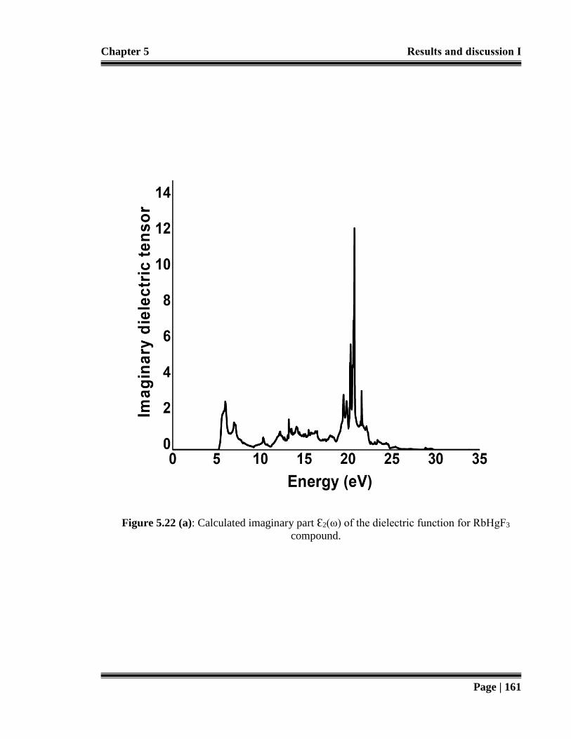
Chapter 5 Results and discussion Ι
Page | 161
Figure 5.22 (a): Calculated imaginary part Ԑ2(ω) of the dielectric function for RbHgF3
compound.

Chapter 5 Results and discussion Ι
Page | 162
Figure 5.22 (b): Calculated real part Ԑ1(ω) of the dielectric function for RbHgF3 compound.

Chapter 5 Results and discussion Ι
Page | 163
Figure 5.22 (c): Calculated absorption coefficient α (ω) of dielectric function for
RbHgF3 compound.

Chapter 5 Results and discussion Ι
Page | 164
Figure 5.22(d): Reflectivity R(ω) as a function of energy for RbHgF3 compound.

Chapter 5 Results and discussion Ι
Page | 165
Table 5.5: Comparison of Present calculation with previous experimental and theoretical
values for lattice constants (ao), ground state energies (Eo), bulk modulus (Bo) and its
pressure derivative (Bp) of RbHgF3 compound.
a) (Muller & Roy 1974), b) (Moreira & Dias 2007)
Compound
RbHgF3
Present
work
————
PBE-GGA
Present
work
————
WC-GGA
Present
work
————
PBEsol-
GGA
Present
work
————
LDA
Experimental
work
Other
theoretical
work
ao (Å)
4.60 4.57 4.53 4.49 4.47a 4.46b
Eo (Ry) -45854.51 -45854.43 -45854.40 -45854.39
Bo (GPa) 48.84 49.01 49.39 49.81 48.32a
BP(GPa) 5.61 5.58 5.53 5.51

Chapter 5 Results and discussion Ι
Page | 166
5.5 Conclusion
In this chapter, systematic first principles calculation of five fluoroperovskites (SrLiF3,
SrNaF3, SrKF3, SrRbF3 and RbHgF3) have been carried out successfully.
Comprehensive results of structural, elastic and mechanical properties of strontium based
group 1A compounds, (section 5.2), reveals that value of lattice constants increases, as cation
shift from Lithium to Rubidium, while value of bulk modulus decreases, that can be
attributed to higher extent of atomic radii of Rubidium. Furthermore, these elastically and
mechanically stable compounds have dominant brittle and ionic behavior.
Section 5.3 delivers unique theoretical strategy to calculate detailed opto-electronic trends of
strontium based group 1A fluoroperovskites, via various exchange and correlation schemes,
provides accurate description of band profiles, which permits to investigate reliable
predictions of electronic charge density and density of states. These calculations argue
against the existence of low bandgap values that have been studied previously with less
reliable Local Density Approximation (LDA) and Generalized Gradient Approximation
(GGA) schemes but there is lack of experimental data so in description we compare Tran-
Blaha modified Becke–Johnson (TB-mBJ) band gap results that are generally similar to
experimental band profile of BaLiF3 compounds. On the basis of above exploration, it can be
concluded that SrMF3 (M= Li, Na, K, Rb) are ionic, wide, and direct bandgap
fluoroperovskites and need an extensive experimental research for their possible utilization in
Ultra-Violet (UV) transparent lens material and in advanced lithographic technology.
In section 5.4, structural, and opto-electronic properties of RbHgF3 have been discussed, with
four different exchange-correlation approximations. The analysis of energy band profiles

Chapter 5 Results and discussion Ι
Page | 167
authenticates indirect narrow energy bandgap (M–Γ) semi-conductive nature. While
contribution of different bands ensures mixed covalent, and ionic behavior. The
advantageous optical responses explore wide range of absorption and reflection in high
frequency regions. Hence RbHgF3 can be efficiently applied for manufacturing high class
lens material with low birefringence and by suitable doping can be utilized in photovoltaic
applications as well.

Chapter 6 Results and discussion ΙΙ
Page | 168
Chapter 6: Results and discussion ΙΙ;
Investigation of mechanical and optoelectronic behavior of
actinoid based oxide perovskites
“Prediction is very difficult,
Especially about the future.”
Niels Bohr
6.1 Introduction
Now-a-days faster, flexible and efficient devices are attaining huge attention. In this regard,
material scientists are struggling hard for reconnoitering new materials. In the last few
decades, much interest has been given to perovskite oxides which have large value of static
dielectric constants. Materials possessing greater value than that of silicon, (for silicon Ԑ0 = 7)
can be classified in terms of high dielectric constant materials. In fact, Ԑ0 have the ability to
decide about miniaturization extent of any material and this idea can be ultimately utilized in
integrated device synthesis.
In section 6.2 potassium and rubidium based protactinium oxide perovskites are investigated
to explore their possible aspects. Technically XPaO3 (X = K, Rb) compounds are sound but
due to radio-active nature and high cost of protactinium, little systematic investigation has
been stated on them. So, this theoretical work motivated us to inquire XPaO3 in detail. In the
present work, to address significant aspects various physical properties of XPaO3 are
explored for their possible technological applications.
The section 6.3 of this chapter is dedicated to inquire Ba based oxide perovskites BaPaO3 and
BaUO3 that fall in the class of high dielectric constant materials (Erum and Iqbal, Februrary
2017) but experimental as well as theoretical information are unavailable due to radioactive
Chapter 6 Results and discussion ΙΙ
Page | 169
nature of these compounds. So, in this study aim is to contribute on scientific information of
these compounds which are equally important to investigate about possible properties such as
electronic structure, elastic behavior, mechanical stability, opto-electronic and dielectric
properties on them.
6.2 Mechanical and optoelectronic study of XPaO3 (X= K, Rb)
The crystal structure of both KPaO3 and RbPaO3 have been reported as an ideal cubic
perovskites-type structure. The first experimental report about these compounds was the
work of Keller (Keller 1965). He reported that these systems have cubic perovskite structure
with the lattice constants 4.341 Å and 4.368 Å for KPaO3 and RbPaO3, respectively. Next
was the work of Iyer and Smith (Iyer and Smith 1971). However, they probably do not obtain
KPaO3, but product which was richer in Pa2O5 rather than KPaO3. It seems that, the work of
Keller (Keller 1965) is the only experimental report so far in which cubic KPaO3 and
RbPaO3 have been obtained.
6.2.1 Structural properties
As mentioned in literature survey that ternary oxide perovskites KPaO3 and RbPaO3, have
space group Pm-3m (no. 221) crystallizes in simple cubic structure. The cubic unit cell
crystal structure is displayed in Figure 6.1 (a) and 6.1 (b) for KPaO3 and RbPaO3,
respectively. The total energy is determined at various volumes as illustrated by Figure 6.2
(a) and 6.2 (b) for KPaO3 and RbPaO3, correspondingly. The XPaO3 structural aspects are
calculated by same energy minimizing process as mentioned in section 5.2 of chapter 5
(Murnaghan 1944). In which corresponding equilibrium unit cell volume and total energy are
evaluated by corresponding set of various lattice parameters. The details of resultant lattice

Chapter 6 Results and discussion ΙΙ
Page | 170
parameters calculated from GGA and LDA approximations are shown in Table 6.1. That
reveals value of lattice constant for RbPaO3 is larger than KPaO3 and vice versa, and it can
be clarified in terms of following relation R(K) = 2.43 Å is smaller than that of R(Rb) =
2.65 Å.
Furthermore, to clarify this chemistry two analytical methods are also employed to calculate
lattice constants. Both ionic radii and Verma Jindal calculation of lattice constants are based
on equations 6.1 and 6.2 respectively,
a0 = α + β (rX + rO) + Ɣ(rPa + rO) (6.1)
a0 = K(VXVPaVO)srav (6.2)
using ionic radii of rK = 1.64 Å, rRb = 1.72 Å, rPa = 0.90 Å, and ro = 1.35 Å, for K, Rb, Pa, and
O correspondingly, with valence electrons of 1, 2 and 6 for X, Pa, and O. Due to the
dependence of equations 6.2 on the number of valence electrons, the calculated lattice
constants via V.J method illustrates deviation within 7-8 % while for I.R methods this
deviation is within 2-3% with respect to DFT method but experimental versus DFT
calculated outcomes are in reasonable similarity by each other. Crystal rigidity of XPaO3 are
estimated with the help of bulk modulus value. It can be manipulated from Table 6.1 that
RbPaO3 have smaller value of bulk modulus than KPaO3 in contrary relation with value of
lattice constant. The same contrary relation between bulk modulus and lattice constant have
been found for another perovskite reported previously by Gheloubi with his fellows
(Gheloubi et al., 2012), as well as by Erum and Iqbal (Erum and Iqbal, March 2017).

Chapter 6 Results and discussion ΙΙ
Page | 171
The interpretation of chemical bonding is performed with chemical trends. Further this
structural chemistry is used to estimate tolerance factor, where the length or distance between
the two bonded atoms is well known as bond length. It can be noticed from Table 6.1 as
KPaO3 approaches to RbPaO3, there is increment between bond lengths of X and O atoms.
Furthermore, for X, Pa, and O, similar trend is observed. Next, we evaluate the criteria of
tolerance factor by using bond length for XPaO3 compounds (Goldschmidt 1926).
𝑡 =0.707<𝑋−0>
<𝑃𝑎−𝑂> (6.3)
In above equation <Pa-O> and <X-O> depicts X, O and Pa respectively, which satisfies good
tolerance factor criteria within 0.93-1.02 as presented in Table 6.2.
6.2.2 Elastic constant calculations
Elastic properties give reliable information regarding to stability of structure and binary
chemistry (Sadd 2005). In Table 6.3, three major elastic constants are summarized which are
C11, C12 and C44 respectively. All these calculations are carried out by using Charpin’s
method (Charpin 2001). As this is first theoretical approach for calculating elastic constants
of XPaO3 compounds, so this work can be a comparative approach for other scientists
working on the same direction. To ensure cubic as well as mechanical stability, it is a good
finding that all elastic constants satisfy condition of traditional mechanical stability at
pressure of 0 GPa. The details of traditional mechanical stability condition can be found in
our recent paper authored by Erum and Iqbal (Erum and Iqbal 2016). For KPaO3 the
resistance for unidirectional compression is high (432.182 GPa) along the (principle)
crystallographic direction while it possesses a lower value (311.413 GPa) for RbPaO3, which
validates the weak unidirectional resistance for KPaO3 compound. Meziani and Belkhir
(Meziani and Belkhir 2012) observed the similar results for C11 elastic constant. The results

Chapter 6 Results and discussion ΙΙ
Page | 172
of C44 which is shear or volumetric deformation reveals that both compounds retains greater
resistance for compression rather than shear deformation.
6.2.3 Mechanical parameters
The purpose of this section is to compute polycrystalline mechanical aspects by utilizing data
information from elastic constants. The evaluated parameters include detailed elastic moduli,
Poisson’s ratio, coefficients for elastic stiffness, and melting temperature.
6.2.3.1 Elastic moduli calculations
The hardness of material is an important entity which can use to estimate rigidity of any
crystalline structure. For this purpose, shear and bulk modulus are equally employed which
can conveniently be explored by Voigt Reuss-Hill (VRH) approximation (Reuss and Angew
1929; Shafiq et al., 2015):
𝑮𝑽 = 𝟏
𝟓(𝑪𝟏𝟏 − 𝑪𝟏𝟐 + 𝟑𝑪𝟒𝟒), (6.4)
𝑮𝑹 =𝟓𝑪𝟒𝟒(𝑪𝟏𝟏−𝑪𝟏𝟐)
𝟒𝑪𝟒𝟒+𝟑(𝑪𝟏𝟏−𝑪𝟏𝟐) , (6.5)
𝑮 =𝑮𝑽+𝑮𝑹
𝟐 , (6.6)
𝑩 =𝟏
𝟑 (𝑪𝟏𝟏 + 𝟐𝑪𝟏𝟐) (6.7)
For shear and bulk modulus, it can be noticed from Table 6.4 that KPaO3 (70.25 GPa, 203.78
GPa) have larger value than that RbPaO3 (69.48GPa, 146.98GPa) respectively. The
contribution of material for linear strain is estimated through Young’s modulus by (Kittel
2005):
𝒚 =𝟗𝑩𝑮
(𝟑𝑩+𝑮). (6.8)

Chapter 6 Results and discussion ΙΙ
Page | 173
RbPaO3 has lower values for shear, bulk and Young’s modulus rather than KPaO3 which
depicts lower tendency of charge transfer among cation and anion respectively. Next to
identify the correct information regarding to brittle/ flexible or ductile character of XPaO3,
the criteria for B/G ratio is evaluated. Typical values of B/G less than 1.75 and greater than
1.75 refers material to be brittle or ductile/flexible (Pugh 1954). The calculated B/G values
(2.901 GPa, 2.120 GPa) for KPaO3, and RbPaO3 confirms strong flexibility of respective
compounds.
6.2.3.2 Cauchy’s pressure and Poisson’s ratio calculations
Next, the Cauchy’s pressure is utilized to confirm flexible nature by taking difference
between C12 and C44 elastic constant respectively. If the value of this particular pressure is
negative/ positive, then material tend towards brittle/flexible in nature (Brik 2011), as shown
in Table 6.5:
𝑪′′ = 𝑪𝟏𝟐 − 𝑪𝟒𝟒 . (6.9)
Meanwhile according to Frantsevich and his fellows (Frantsevich et al., 1983), if material
retains Poisson’s ratio v > 0.26 than material will dominate with flexible characteristics, as
shown in Table 6.5:
ѵ =(𝟑𝑩−𝟐𝑮)
𝟐(𝟑𝑩+𝑮) (6.10)
At this point, it can be observed that for both compounds 𝐶′′ > 0, v > 0.26 and B/G > 1.75
indicates that XPaO3 contains high directional bonding and is flexible in nature.
6.2.3.3 Shear constant and elastic anisotropy calculations
Next the shear constant is calculated to differentiate bonding characteristic (Nakamura 1995),
as shown in Table 6.5:
𝑪′ =𝟏
𝟐(𝑪𝟏𝟏 − 𝑪𝟏𝟐) (6.11)
Chapter 6 Results and discussion ΙΙ
Page | 174
High value of shear constant reveal that XPaO3 contains dominant covalent behavior. The
isotropic behavior of any crystal in manufacturing disciplines can be estimated through
elastic anisotropy parameter “A” (Jamal et al., 2016), as shown in Table 6.5:
𝑨 =𝟐𝑪𝟒𝟒
(𝑪𝟏𝟏−𝑪𝟏𝟐). (6.12)
Cubic crystals can be completely categorized by means of anisotropic factor (A), if A is
equivalent to unity, then material is isotropic but present calculations notified that it deviates
from 1 so XPaO3 can be completely characterized as anisotropic class of compounds because
of deviation of its value from unity.
6.2.3.4 Lame’s constant calculations
Next, the study is related with stress to strain by acknowledging two important constants
namely first λ and second μ Lame’s constant. The expression for these constants can be
derived from various mechanical parameters in the following form (Alouani 1991):
𝝀 = 𝒀ѵ
(𝟏+ѵ)(𝟏−𝟐ѵ) (6.13)
𝝁 =𝒀
𝟐(𝟏+ѵ) (6.14)
Above equations reveals that these constants are in direct relation with the value of Y. Our
calculated values not fulfill the specific criteria λ = C12 and μ = C′ for isotropic material.
So XPaO3 is a class of anisotropic compounds which is in accordance with the calculated
value of anisotropy parameters as well.
6.2.3.5 Melting temperature calculations
Another important factor is melting temperature (Tm) that elaborates the extent of melting for
a specified material via following relation (Fine et al., 1984):
Tm = 607 + 9.3B + 555 (6.15)

Chapter 6 Results and discussion ΙΙ
Page | 175
Table 6.5 shows that RbPaO3 have lower tendency of melting rather than KPaO3.
6.2.4 Electronic behavior
In this section electronic behavior of XPaO3 are evaluated by electronic band structure, by
evaluating density of states (DOS) as well as bonding nature is calculated via contour maps
of electron density from Tran-Blaha modified Becke–Johnson (TB-mBJ) potential (Tran and
Blaha 2009).
6.2.4.1 Band structure calculations
At this point of investigation, band structure comparison of XPaO3 at different symmetry
points with various approximations are presented in Table 6.6. It can be observed that at all
symmetry points except (Γ-Γ), gap value is high. Though pictorial demonstration of band
structure with (TB-mBJ) at Brillouin Zone are displayed in Figure 6.3. The XPaO3
compounds without any external pressure reveals (Γ-Γ) symmetry direct bandgap of about
3.60 eV and 3.14 eV for KPaO3 as well as RbPaO3 correspondingly. These materials have
larger bandgap than 3.1 eV, so work well for ultraviolet region of (electromagnetic) spectrum
(Lang 2014).
6.2.4.2 Density of States (DOS) calculations
The computation of partial and total density of states is complementary to calculate
accessible number of positions to occupy. From Figure 6.4 (a) and 6.4 (b), it can be observed
that total interval of energy encompasses region of fermi level EF from (EF – 20eV) up to (EF
+ 15eV). However, appearance of sharp peak due to O 2s state is observed at (EF – 20eV).
Then 5p states of Pa, dominate the energy interval at (EF - 15eV). After fermi level to -4.6 eV
(the upper valence band region) dominates via O-2p states whereas Pa-4f states occupies

Chapter 6 Results and discussion ΙΙ
Page | 176
conduction band till 6 eV approximately. As a result, formation of conduction band is
because of mixed of X: 3d and Pa: d states.
6.2.4.3 Electron density contour calculations
In crystalline solids, the nature of bonding can be analyzed by contour maps of electron
density (Gelatt 1983). From (110) plane charge densities between X, Pa, O atoms can be
observed as shown in Figure 6.6 and 6.7, for two as well as three dimensions respectively.
However, from view of (100) plane contour plots of just corresponding X and O ions can be
seen as displayed in Figure 6.5 and 6.8, for two as well as three dimensions respectively. It
can be observed that between X and O ions the nature of bonding is ionic, since of the fact
that very low hybridization occurs between X-O ions. However, there is large sharing
between Pa and O ion, which depicts strong covalent character and it is well known reality
that hybridization between cations and anions causes covalent nature of respective
compounds (Erum and Iqbal, February 2017).
6.2.5 Optical characteristics
This part of the chapter is dedicated to compute, the optical properties of XPaO3 compounds
by means of Trans-Blaha modified Becke–Johnson (TB-mBJ) potential. The basic optical
parameter covers imaginary part of dielectric function Ԑ2(ω), real part of dielectric function
Ԑ1(ω), extinction coefficient k(w), absorption coefficient α(ω), reflectivity R (ω), optical
conductivity σ(ω), energy loss function L(ω), and effective number of electrons neff via sum
rules.
6.2.5.1 Complex dielectric constant calculations
Here complex part of dielectric function can be written as (Fox 2001):

Chapter 6 Results and discussion ΙΙ
Page | 177
Ԑ(𝜔) = Ԑ1(𝜔) + 𝑖Ԑ2(𝜔) (6.16)
First part of equation denotes real part Ԑ1(ω) while second part of above equation represents
imaginary part Ԑ2(ω). The Ԑ1(ω) can be used to express comprehensive response of a
compound via following equation (Wooten 1972):
Ԑ2(𝜔) = (4𝜋2𝑒2
𝑚2𝜔2) ∑ ∫ ⟨𝑖|𝑀|𝑗⟩2𝑓𝑖(1 − 𝑓𝑖)𝛿(𝐸ј,𝑘 − 𝐸𝑖,𝑘 − 𝜔)
𝑘𝑖,𝑗 𝑑3𝑘. (6.17)
In above equation M, 𝑓𝑖, 𝐸𝑖,𝑘 and 𝐸ј,𝑘 are diploe matrix, i-th state fermi distribution function,
and i-th as well as j-th state energy of electron correspondingly. Ԑ2(ω) peaks represents
perfect outline of band structure and DOS respectively. As shown in Figure 6.9 (a) critical
point of threshold occurs at about 3.99 eV and 3.81 eV for RbPaO3 and KPaO3 accordingly.
However, occurrence of principle peak occurs due to Pa-4f at about 6 eV for XPaO3, which
refers towards transition between states of valence band (occupied) to conduction band
(unoccupied). After that till 15 eV diversified peaks are observed due to overlapping of states
between X-3d and few d plus p states of Pa and O respectively.
The polarization phenomenon can be observed by Ԑ1(ω) through subsequent relation (Brik
2011):
Ԑ1(𝜔) = 1 +2
𝜋𝑃 ∫
ὠԐ2(ὠ)𝑑ὠ
ὠ2−ὠ2
ⱷ
0 , (6.18)
Here principle value of corresponding integral is denoted by P. It can be observed from
Figure 6.9 (b) that the dielectric function Ԑ1(0), the static part, noticed at about 4.5 eV for
both compounds. The Ԑ1(ω) curves starts increasing and achieves their extreme rate nearby
3.7 eV for XPaO3.

Chapter 6 Results and discussion ΙΙ
Page | 178
6.2.5.2 Optical conductivity and energy loss calculations
The calculated values of complex dielectric function Ԑ(ω) can allow to determine key optical
function for the electromagnetic spectrum such as optical conductivity σ(ω), and electron
energy loss spectrum L(ω) which can be determined by following expressions (Fox 2001):
𝜎(𝜔) = 2𝑊𝐶𝑉ℏ𝜔
𝐸02 (6.19)
𝐿(𝜔) = 𝐼𝑚 (−1
Ԑ(𝜔)) (6.20)
The journey of optical conductivity σ(ω) reveals that it starts at approximately 2 eV with
minor mounting peaks, then ultimately attain highest peak at about 6 eV for XPaO3 as
displayed in Figure 6.9 (c). A prominent fact can be observed from σ(ω) that it shifts towards
high energy region as compound traversed from K to Rb due to increase in band width of the
corresponding compound. The characteristic contribution of plasma resonance frequency ωp
can be depicted with the help of energy loss function L(ω) (Murtaza and Ahmad 2012).
Figure 6.9 (d) reveals for both compounds a prominent crest is detected at about 10 eV.
6.2.5.3 Refractive index and reflectivity calculations
The key optical parameters such as refractive index n(ω), and reflectivity R can be
determined by following expressions (Wooten 1972):
𝑛(𝜔) = 1
√2[√Є1(𝜔)2 + Є2(𝜔)2 + Є1(𝜔) ]
1
2 (6.21)
𝑅 = |𝑛−1
𝑛+1|
2
(6.22)

Chapter 6 Results and discussion ΙΙ
Page | 179
In Figure 6.9 (e) and 6.9 (f), the calculated spectrum of refractive index as well as reflectivity
are shown. The refractive index (static parts) n (0) for KPaO3 and RbPaO3 are at value of
2.07 and 2.09 respectively. The maxima in values of refractive index attains at 4 eV (2.81)
and 4.1eV (2.82) for KPaO3 and RbPaO3 respectively. However, Figure 6.9 (f) depicts that
XPaO3 initiates high reflection and acquires maxima in 23-27 eV range. So, in this specific
range, materials show high transparency.
6.2.5.4 Absorption coefficient calculations
The absorption coefficient α (ω) can be calculated via following relations (Harmel et al.,
2015):
𝛼(𝜔) =4𝜋ƙ(𝜔)
𝜆 (6.23)
From the plot of Figure 6.9 (g) (plot of absorption coefficient α (ω)), it can be observed that
XPaO3 starts absorption phenomenon at about 4.25 eV. The particular point of threshold is in
similar resemblance with the behavior of bandgap trends, along with effective absorption
occurs in 21-25 eV range. After the incent of highest peak diversified small and large peaks
are observed till 30 eV. The wide range of absorption suggests use of XPaO3 in absorption
purpose applications, characteristically nearby 23 eV.
6.2.5.5 Sum rules calculation via neff
In the end, the sum rule is evaluated to consider the number of effective valence electrons via
corresponding formula (Abelès 1972):
𝑛𝑒𝑓𝑓(𝜔) = ∫ 𝜎(ὠ)𝜔
0ὠ 𝑑ὠ (6.24)

Chapter 6 Results and discussion ΙΙ
Page | 180
Finally, sum rule is evaluated to estimate effective valence electron, which are available to
utilize inter and intra band transitions, appear at about 3.5 eV as figured in Figure 6.9 (h).
The trend-line follow slow, then linear rise in effective number of electrons. Then there
occurs a sharp peak in a region of 12-14 eV, showing saturation of electrons.

Chapter 6 Results and discussion ΙΙ
Page | 181
Figure 6.1(a): Cubic crystal structure of KPaO3

Chapter 6 Results and discussion ΙΙ
Page | 182
Figure 6.1(b): Cubic crystal structure of RbPaO3

Chapter 6 Results and discussion ΙΙ
Page | 183
Figure 6.2 (a): Variations of total energy (E, in Ry) with unit cell volume (V, in (a.u)3)
For KPaO3.
Volume (a.u)3
To
tal
ener
gy
(R
y)

Chapter 6 Results and discussion ΙΙ
Page | 184
Figure 6.2 (b): Variations of total energy (E, in Ry) with unit cell volume (V, in (a.u)3)
for RbPaO3.
Volume (a.u)3
To
tal
ener
gy
(R
y)

Chapter 6 Results and discussion ΙΙ
Page | 185
Figure 6.3: Electronic energy dispersion curves for (a) KPaO3 and (b) RbPaO3 along some
high symmetry directions in the Brillouin zone (BZ) within modified Becke-Johnson (mBJ)
Potential.
En
ergy
(eV
)
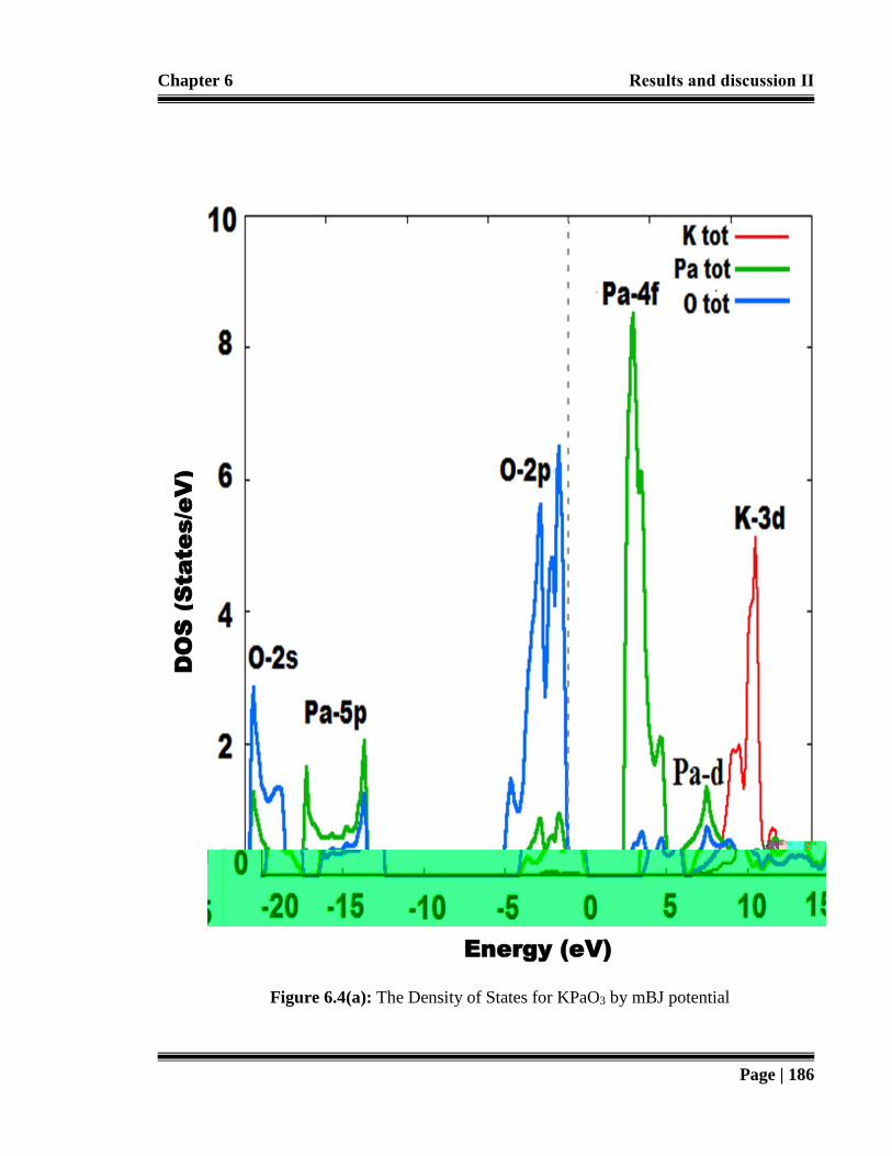
Chapter 6 Results and discussion ΙΙ
Page | 186
Figure 6.4(a): The Density of States for KPaO3 by mBJ potential
Energy (eV)
DO
S (
Sta
tes/e
V)

Chapter 6 Results and discussion ΙΙ
Page | 187
Figure 6.4(b): The Density of States for RbPaO3 by mBJ potential
Energy (eV)
DO
S (
Sta
tes/e
V)

Chapter 6 Results and discussion ΙΙ
Page | 188
Figure 6.5 (a): Calculated mBJ total two and three-dimensional electronic charge densities
for KPaO3 in (100) plane.
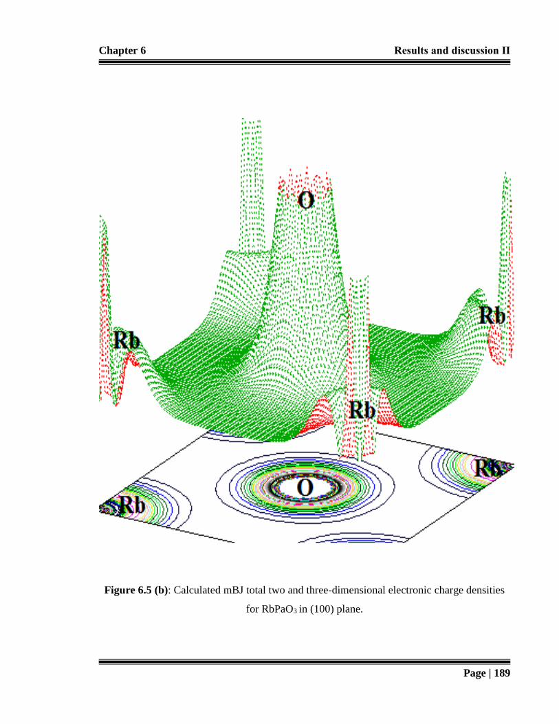
Chapter 6 Results and discussion ΙΙ
Page | 189
Figure 6.5 (b): Calculated mBJ total two and three-dimensional electronic charge densities
for RbPaO3 in (100) plane.

Chapter 6 Results and discussion ΙΙ
Page | 190
Figure 6.6 (a): Calculated mBJ total two and three-dimensional electronic charge densities
for KPaO3 in (110) plane.

Chapter 6 Results and discussion ΙΙ
Page | 191
Figure 6.6 (b): Calculated mBJ total two and three-dimensional electronic charge densities
for RbPaO3 in (110) plane.

Chapter 6 Results and discussion ΙΙ
Page | 192
Figure 6.7: Total two-dimensional electron density plots in (110) plane for (a) KPaO3,
(b) RbPaO3.
Figure 6.8: Total two-dimensional electron density plots in (100) plane for (a) KPaO3,
(b) RbPaO3.

Chapter 6 Results and discussion ΙΙ
Page | 193
Figure 6.9(a): Calculated imaginary part Ԑ2(ω) of the dielectric function for
XPaO3 (K, Rb) compounds.

Chapter 6 Results and discussion ΙΙ
Page | 194
Figure 6.9 (b): Calculated real part Ԑ1(ω) of the dielectric function for
XPaO3 (K, Rb) compounds.

Chapter 6 Results and discussion ΙΙ
Page | 195
Figure 6.9 (c): Calculated conductivity σ(ω) for XPaO3 (K, Rb) compounds.

Chapter 6 Results and discussion ΙΙ
Page | 196
Figure 6.9 (d): Calculated energy loss function L (ω) for XPaO3 (K,Rb) compounds.

Chapter 6 Results and discussion ΙΙ
Page | 197
Figure 6.9 (e): Refractive index n (ω) as a function of energy for XPaO3 (X=K, Rb)
compounds.

Chapter 6 Results and discussion ΙΙ
Page | 198
Figure 6.9 (f): Reflectivity R (ω) as a function of energy for XPaO3 (X=K, Rb)
compounds.

Chapter 6 Results and discussion ΙΙ
Page | 199
Figure 6.9 (g): Absorption coefficient α (ω) as a function of energy for XPaO3 (X=K, Rb)
compounds

Chapter 6 Results and discussion ΙΙ
Page | 200
Figure 6.9 (h): Calculated sum rule (Neff) for XPaO3 (K, Rb) compounds.

Chapter 6 Results and discussion ΙΙ
Page | 201
Table 6.1: Comparisons of calculated values of bond length, equilibrium lattice constant (ao
in Ǻ), ground state energy (Eo in RY), bulk modulus (Boin GPa) and its pressure derivative
(BP) with experimental and other theoretical results for XPaO3 (X = K, Rb) compounds.
a) (Muller & Roy 1974) b) (Morss et al., 2010) c) (Jain et al., 2013) (Experimental Work), d) (Majid and Lee
2010), e) (Verma et al.,2008), f) (Jiang 2006), g) (Moreira and Dias 2006) (Other theoretical work)
Compound Present work
——————— GGA
Present work
—————
——
LDA
Present Analytical
work
———————
I.R method
Present Analytical
work
———————
V.J method
Experimental
work
Other
theoretical
work
KPaO3
ao (Å)
4.37 4.32 4.29 3.99 4.34a,4.36b,
4.38c 4.34d,4.32d, 4.18e,4.24f,
4.23g
Eo (Ry) -56260.653 -56260.713
Bo (GPa) 203.51 203.63
BP(GPa) 3.99 3.98
Bond-
lengths
K-O(Å) 2.51
K-Pa(Å) 3.23
Pa-O(Å) 1.81
RbPaO3
ao (Å)
4.42 4.35 4.32 4.05 4.37a,4.40b,
4.39c
4.36d,4.37d,
4.27e,4.26f,
4.26g
Eo (Ry) -60982.210 -60982.279
Bo (GPa) 146.58 146.65
BP(GPa) 4.122 4.291
Bond-
lengths
Rb-O(Å) 2.61
Rb-Pa(Å) 3.81
Pa-O(Å) 1.82
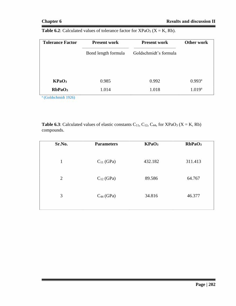
Chapter 6 Results and discussion ΙΙ
Page | 202
Table 6.2: Calculated values of tolerance factor for XPaO3 (X = K, Rb).
a (Goldschmidt 1926)
Table 6.3: Calculated values of elastic constants C11, C12, C44, for XPaO3 (X = K, Rb)
compounds.
Tolerance Factor Present work
——————————
Bond length formula
Present work
—————————
Goldschmidt’s formula
Other work
KPaO3 0.985 0.992 0.993a
RbPaO3 1.014 1.018 1.019a
Sr.No. Parameters KPaO3 RbPaO3
1 C11 (GPa) 432.182 311.413
2 C12 (GPa) 89.586 64.767
3 C44 (GPa) 34.816 46.377

Chapter 6 Results and discussion ΙΙ
Page | 203
Table 6.4: Calculated values of Bulk modulus B0, Reuss’s shear modulus GR, Voigt’s shear
modulus GV, Hill’s shear modulus GH, Young’s modulus Y and Pugh’s index of ductility
Bo/GH.
Sr.No. Parameters KPaO3 RbPaO3
1 Bo(GPa) 203.785 146.982
2 GR(GPa) 51.101 61.802
3 Gv(GPa) 89.408 77.155
4 GH(GPa) 70.254 69.478
5 Y (GPa) 189.038 180.06
6 Bo/GH (GPa) 2.901 2.120

Chapter 6 Results and discussion ΙΙ
Page | 204
Table 6.5: Calculated values of Shear constant (C′), Cauchy pressure (C′′), Lame’s
coefficients (λ and μ), Anisotropy constant (A in GPa) and Poisson’s ratio (ѵ in GPa) and the
melting temperature (Tm in K) for XPaO3 (X= K, Rb) compounds.
Sr.No. Parameters KPaO3 RbPaO3
1 C′ 171.29 123.32
2 C′′ 54.77 18.39
3 Ѵ (GPa) 0.35 0.30
4 A (GPa) 0.20 0.38
5 λ 156.77 100.04
6 μ 70.27 69.52
7 Tm(K) 3057 2529

Chapter 6 Results and discussion ΙΙ
Page | 205
Table 6.6: Band gap comparison of XPaO3 (X = K, Rb) at different symmetry points.
Compound Symmetry
Point
Bandgap
Type 𝐄𝐠
𝐌𝐁𝐉(eV) 𝐄𝐠
𝐋𝐃𝐀(eV) 𝐄𝐠𝐖𝐂−𝐆𝐆𝐀(eV) 𝐄𝐠
𝐏𝐁𝐄−𝐆𝐆𝐀(eV) 𝐄𝐠𝐏𝐁𝐄𝐬𝐨𝐥−𝐆𝐆𝐀(eV)
KPaO3 Γ-Γ Direct 3.60 3.41 3.51 3.49 3.45
R-R Direct 4.41 4.22 4.33 4.31 4.27
M-M Direct 4.45 4.32 4.42 4.39 4.36
X-X Direct 4.39 4.21 4.31 4.29 4.26
RbPaO3 Γ-Γ Direct 3.14 2.93 3.04 3.01 2.97
R-R Direct 3.38 3.27 3.34 3.31 3.29
M-M Direct 3.42 3.21 3.39 3.37 3.23
X-X Direct 3.21 2.98 3.18 3.12 3.10

Chapter 6 Results and discussion ΙΙ
Page | 206
6.3 Ab initio study of high dielectric constant BaMO3 (M=Pa, U)
oxide perovskite
In some earlier experimental studies BaUO3 has been quite successfully explored, in which
enthalpies of formation and calculation of molar Gibbs energy by solution calorimetric
analysis are evaluated (Williams et al. 1984 & Deacon-Smith 2015). In another, study
thermochemical and thermoelectric properties have been investigated successfully (Chen et
al., 1999 & Kurosaki 2001).
6.3.1 Structural parameters
The crystals of BaMO3 (M=Pa, U) perovskite oxides crystallizes in Pm-3m (no. 221) space
group having ideal cubic structure as shown in Figure 6.10 (a)-6.10 (b) for BaPaO3 and
BaUO3 respectively. The sites of Wyckoff coordinates are positioned at (0 0 0), (1/2,
1/2,1/2), (1/2, 1/2, 0) for Ba, X= (Pa, U) and O atoms respectively. In order to achieve,
optimum volume for BaMO3, total energy is determined at various volumes by utilizing
equation of state proposed by Murnaghan (Murnaghan 1944). The optimization plots of each
compound are displayed Figure 6.11 (a) and 6.11 (b) respectively. The calculated optimized
ground state structural parameters lattice constants (ao), bulk moduli (Bo), and ground state
energies (Eo) are tabulated in Table 6.7. The optimized lattice parameters are also compared
with experimental and previous theoretical results.
In this section, lattice constants are also evaluated by two well-known analytical methods
namely ionic radii and Verma Jindal method. The formula for ionic radii method can be
interpreted as (Clementi et al., 1963):
𝑎0 = 𝛼 + 𝛽 (𝑟𝐵𝑎 + 𝑟𝑂) + Ɣ(𝑟𝑋 + 𝑟𝑂) (6.25)

Chapter 6 Results and discussion ΙΙ
Page | 207
Where rBa, rX (x= Pa,U) and rO are ionic radii for Ba (1.61 A0), Pa (0.90 A0), U (0.89 A0) and O
(1.35 A0) respectively. Verma and Jindal model depends upon the average ionic radii and
number of valence electrons as follows (Verma et al., 2008):
𝑎0 = 𝐾(𝑉𝑋𝑉𝑃𝑎𝑉𝑂)𝑠𝑟𝑎𝑣 (6.26)
Where average ionic radii are denoted by rav and 2, 2, while 6 are number of valence
electrons for Ba (VBa), X (VX) as well as O (VO) correspondingly. While S (0.09) and K
(2.45) are constants for equation. It can be noticed from Table 6.7 that Density Functional
Theory (DFT) and analytical (ionic radii as well as Verma and Jindal method) calculation of
lattice constant reveals some deviation within 2-3 % as compared to experimental results.
Next, the rigidity of crystal structure can be determined in terms of bulk modulus which
depicts, BaPaO3 possesses lower bulk modulus than BaUO3. In addition to it, inverse relation
between bulk modulus as well as lattice constant can be observed which is in similar
accordance with KPaO3 and RbPaO3 perovskite compounds respectively (Erum and Iqbal,
February 2017).
Next part of this section is to determine extent of activation energy for oxygen migration
which can be clearly illustrated by calculating critical radius. In doping selection procedure
critical radius illustrates an imperative part by using following formula (Marezio et al., 1970
& Blundell 2001):
𝑟𝑐 =1.4141𝑟𝑀 −𝑟𝑜 −3.414𝑟𝐵𝑎+5.828(𝑟𝐵𝑎− 𝑟𝑜)2
2𝑟𝐵𝑎+0.828 𝑟𝑀+2.828𝑟𝑜 (6.27)
Table 6.7 explores that BaPaO3 have larger value of critical radius than BaPaO3. So, it can be
concluded that BaUO3 have larger migration energy. The information of important chemical
trends can be estimated by acknowledging bond lengths which are shown in Table 6.7.

Chapter 6 Results and discussion ΙΙ
Page | 208
Further tolerance factor is calculated to interpret structural symmetry in BaMO3 compounds
as follows (Goldschmidt 1926):
𝑡 =0.707<𝐵𝑎−𝑂>
<𝑋−𝑂> (6.28)
Where X, Ba, and O are average lengths of corresponding bonds as shown in Table 6.8.
Both BaPaO3 and BaUO3 satisfy good criteria of tolerance factor for cubic crystal which lies
within 0.93-1.02 range.
6.3.2 Electronic behavior
In this sub-section electronic properties of BaMO3 are investigated with the aid of electronic
band structure, Density of states (DOS) total as well as partial, and electronic charge density
distribution.
6.3.2.1 Band structure calculations
The bandgap results can be observed from Table 6.9 that are computed with four various
types of exchange and correlation schemes of ab-initio study. However, for this thesis
graphical attention is only paid to bandgap by WC-GGA approximation, keeping in mind its
accuracy for metals and semiconductors, as shown in Figure 6.12. It can be observed that
minima of conduction band minima (CBM) and maxima of valence band (VBM) occupies
(Γ-Γ) symmetry point revealing direct bandwidth of 4.05 eV for BaPaO3 and 3.98 eV for
BaUO3, however the trend of overall dispersion curves for bands remains identical. It can be
closely examined, that for both compounds conduction band traverses from fermi level while
valence band are well below the fermi level, which verifies metallic nature in BaXO3.
Furthermore, these materials have larger bandgap than 3.1 eV, so work well for ultraviolet
region of (electromagnetic) spectrum (Lang 2014).

Chapter 6 Results and discussion ΙΙ
Page | 209
6.3.2.2 Density of States (DOS) calculations
The states of density distribution comprises on four different regions from (EF – 20 eV) to
(EF + 15 eV) as shown in Figure 6.13 (a) and 6.13 (b) for BaXO3. The core states are
dominated by X-6p states which occupies a region between -20 to -14.4 eV. After that a
distinct peak is observed at -15 eV due to Ba-4p state, however maxima of valence band due
to O-2p state occurs within the interval of -7 to 4.2 eV respectively. Then 5f states of X plays
a dominant role in overall physical properties of conduction band, which is further hybridized
with some of Ba (F and d states) respectively.
6.3.2.3 Electron density Calculations
A very impact full tool for explaining bonding nature of various atoms in crystalline solid is
through contour maps of charge density (Gelatt 1983). From view of (100) plane contour
plots of just corresponding Ba and O ions can be seen as displayed in Figure 6.14 (a-b) and
6.16, for two as well as three dimensions correspondingly. However, from (110) plane charge
densities between Ba, X, O atoms can be observed as shown in Figure 6.15 (a-b) and 6.17,
for two as well as three dimensions respectively. The spherical charge distribution is
observed for Ba and O atoms, without any overlapping, which helps to justify ionic nature
bonding in BaXO3. Similar ionic nature is observed for Ba and O ions due to low extent of
hybridization between Ba as well as O ions is observed. This similar bonding nature for other
perovskites are also observed by Murtaza and his fellows (Murtaza et al., 2011).
6.3.3 Optical characteristics
In this subsection, fundamental and derived optical responses for BaMO3 (X= Pa, U) are
calculated by WC-GGA approximation.

Chapter 6 Results and discussion ΙΙ
Page | 210
6.3.3.1 Complex dielectric constant calculations
The complex part of dielectric function Ԑ (ω), provides basis for the calculation of all
fundamental optical responses. It can be depicted from Figure 6.18 (a) of Ԑ2(ω) that threshold
point occurs at about origin. Next the transition from unoccupied conduction band states to
occupied valence band states causes a major peak for both compounds which is located
approximately at 0.3-0.4 eV. The existence of these peaks is due to 5f states of X (X= Pa, U)
and these peaks imparts a crucial role in overall internal response of BaMO3. Then till 14 eV,
the steady peaks are observed. From Ԑ2(ω), another important phenomenon of strong
absorption (within 0 to 2 eV) can be observed, which might be due to induced electric field,
that results in large collective excitation of effective mass in the interfaces.
The real part of dielectric function Ԑ1(ω) helps to analyze polarizability of a given material
(Brik 2011). It can be analyzed from Figure 5.18 (b) that the peak for Ԑ1(0) (static dielectric
constant) is 40 and 72 for BaPaO3 and BaUO3 respectively.
The corresponding high value of static dielectric constant in both compounds classifies their
high degree of miniaturization in them. After that a sharp decrease in Ԑ1(ω) curve of BaXO3
is observed, which eventually attains a lowest value approximately at 0.3 - 0.4 eV. As a
whole, till 14 eV a narrow bandgap semi-conductive nature is observed.
6.3.3.2 Optical conductivity calculations
The conduction phenomenon can be interpreted from the plot of optical conductivity σ(ω) as
shown in Figure 6.18 (c) that the phenomenon of optical conduction initiates from origin and
attains maximum position approximately at 0.3-0.4 eV, followed by certain decrease in
oscillations.

Chapter 6 Results and discussion ΙΙ
Page | 211
6.3.3.3 Refractive index and reflectivity calculations
Next the plot of refractive index n(ω) and reflectivity R are calculated. Further, it can also be
revealed from the curve of refractive index n (ω) that it possesses a close relationship with
the trend of Ԑ1(ω). It can be observed from Figure 6.18 (d), n (0) lies at 6.3 for BaPaO3 and
9.0 for BaUO3 respectively. In high energy region curve of n (ω) starts vanishing which
ultimately reflects that studied materials loss transparency beyond certain energy limit and
absorbs photon in high energy region. The reflectivity spectrum, R(ω) demonstrates that in
accordance with Ԑ2(ω), BaXO3 starts reflecting highly from the origin which is less for
BaPaO3 than BaUO3 as displayed in Figure 6.18 (e). The R(ω) spectrum curve suffers trivial
variations followed by optimum reflectivity peaks within region of 7.5 to 8.0 eV respectively.
As per particular reflecting properties of both materials they can be classified as highly
transparent materials in infrared region of electromagnetic spectrum.
6.3.3.4 Sum rules calculation via neff
At the end, sum rule is assessed in terms of effective number of valence electrons per unit
cell (Fox 2001). The curves of sum rules deliver distinguished peak at about 2.0 eV as shown
in Figure 6.18 (f). Then the interband transition of electrons increases slowly that ultimately
saturates at approximately 12-14 eV range respectively.

Chapter 6 Results and discussion ΙΙ
Page | 212
Figure 6.10 (a): Cubic crystal structure of BaPaO3
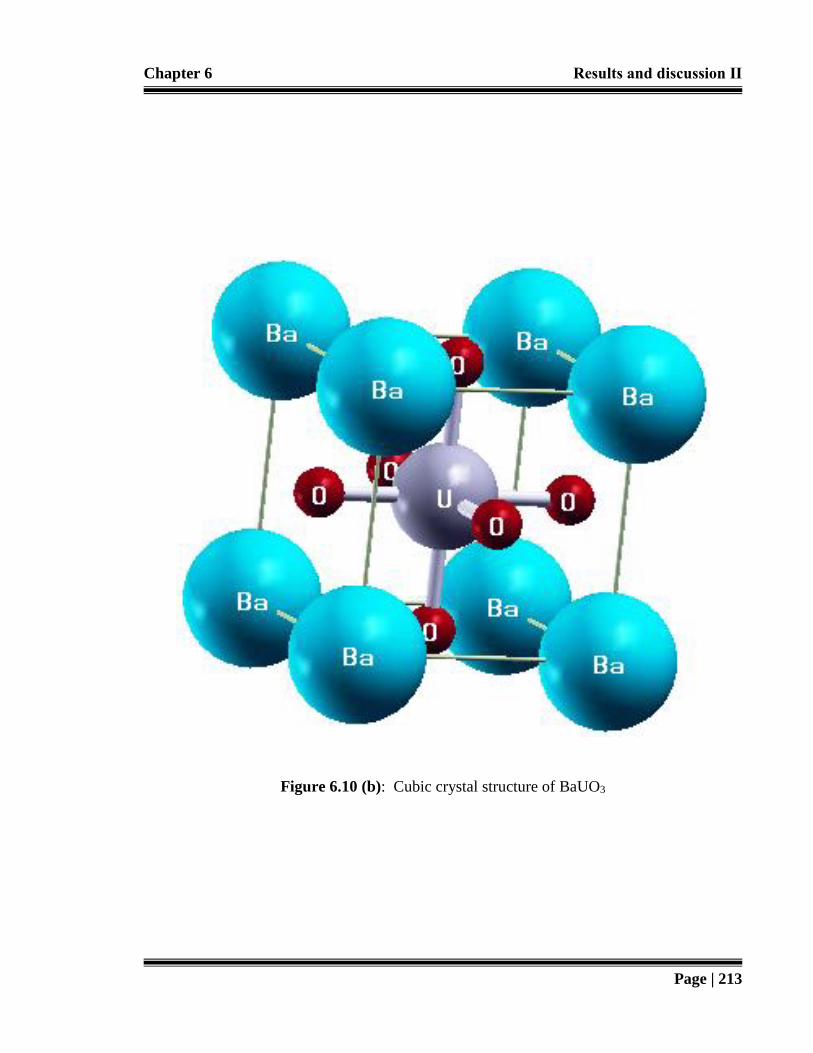
Chapter 6 Results and discussion ΙΙ
Page | 213
Figure 6.10 (b): Cubic crystal structure of BaUO3

Chapter 6 Results and discussion ΙΙ
Page | 214
Figure 5.3: Variations of total energy (E, in Ry) with unit cell volume (V, in (a.u)3) for
KPaO3.
Volume (a.u.)3
En
ergy
(R
y)
Figure 6.11(a): Variations of total energy (E, in Ry) with unit cell volume (V, in
(a.u)3) for BaPaO3.

Chapter 6 Results and discussion ΙΙ
Page | 215
Volume (a.u.)3
En
ergy
(R
y)
Figure 6.11(b): Variations of total energy (E, in Ry) with unit cell volume (V, in
(a.u)3) for BaUO3

Chapter 6 Results and discussion ΙΙ
Page | 216
En
ergy
(eV
)
Figure 6.12: Electronic energy dispersion curves for (a) BaPaO3 and (b) BaUO3 along
some high symmetry directions in the Brillouin zone (BZ) within WC-GGA
approximation.

Chapter 6 Results and discussion ΙΙ
Page | 217
Figure 6.13 (a): The Density of States for BaPaO3 by WC-GGA approximation.
Energy (eV)
DO
S (
Sta
tes/e
V)

Chapter 6 Results and discussion ΙΙ
Page | 218
Figure 6.13 (b): The Density of States for BaUO3 by WC-GGA approximation.
Energy (eV)
DO
S (
Sta
tes/e
V)

Chapter 6 Results and discussion ΙΙ
Page | 219
Figure 6.14 (a): Calculated total two and three-dimensional electronic charge densities for
BaPaO3 in (100) plane.

Chapter 6 Results and discussion ΙΙ
Page | 220
Figure 6.14 (b): Calculated total two and three-dimensional electronic charge densities for
BaUO3 in (100) plane.

Chapter 6 Results and discussion ΙΙ
Page | 221
Figure 6.15 (a): Calculated total two and three-dimensional electronic charge densities for
BaPaO3 in (110) plane.

Chapter 6 Results and discussion ΙΙ
Page | 222
Figure 6.15 (b): Calculated total two and three-dimensional electronic charge densities for
BaUO3 in (110) plane.

Chapter 6 Results and discussion ΙΙ
Page | 223
Figure 6.16: Total two-dimensional electron density plots in (100) plane for (a) BaPaO3,
(b) BaUO3.
Figure 6.17: Total two-dimensional electron density plots in (110) plane for (a) BaPaO3,
(b) BaUO3.

Chapter 6 Results and discussion ΙΙ
Page | 224
Figure 6.18 (a): Calculated imaginary part Ԑ2 (ω) of the dielectric function for
BaXO3 (Pa, U) compounds.

Chapter 6 Results and discussion ΙΙ
Page | 225
Figure 6.18 (b): Calculated real part Ԑ1 (ω) of the dielectric function for
BaXO3 (Pa, U) compounds.

Chapter 6 Results and discussion ΙΙ
Page | 226
Figure 6.18 (c): Calculated conductivity σ (ω) for BaXO3 (X=Pa, U) compounds.
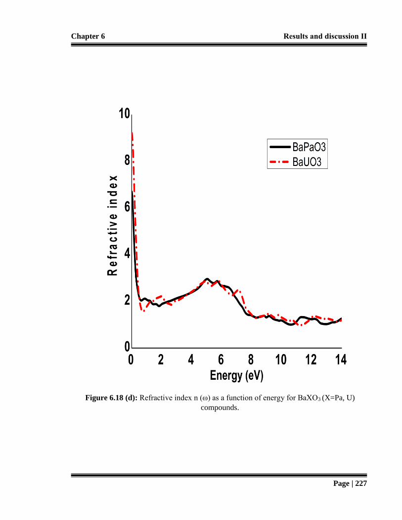
Chapter 6 Results and discussion ΙΙ
Page | 227
Figure 6.18 (d): Refractive index n (ω) as a function of energy for BaXO3 (X=Pa, U)
compounds.

Chapter 6 Results and discussion ΙΙ
Page | 228
Figure 6.18 (e): Reflectivity R (ω) as a function of energy for BaXO3 (Pa,U) compounds.

Chapter 6 Results and discussion ΙΙ
Page | 229
Figure 6.18 (f): Calculated sum rule (Neff) for BaXO3 (Pa,U) compounds.
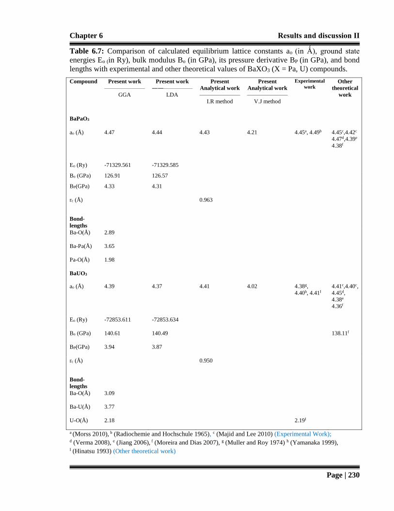
Chapter 6 Results and discussion ΙΙ
Page | 230
Table 6.7: Comparison of calculated equilibrium lattice constants ao (in Ǻ), ground state
energies Eo (in Ry), bulk modulus Bo (in GPa), its pressure derivative BP (in GPa), and bond
lengths with experimental and other theoretical values of BaXO3 (X = Pa, U) compounds.
a (Morss 2010), b (Radiochemie and Hochschule 1965), c (Majid and Lee 2010) (Experimental Work); d (Verma 2008), e (Jiang 2006), f (Moreira and Dias 2007), g (Muller and Roy 1974) h (Yamanaka 1999),
I (Hinatsu 1993) (Other theoretical work)
Compound Present work
———————
GGA
Present work
――—————
LDA
Present
Analytical work
———————
I.R method
Present
Analytical work
———————
V.J method
Experimental
work Other
theoretical
work
BaPaO3
ao (Å)
4.47 4.44 4.43 4.21 4.45a, 4.49b 4.45c,4.42c
4.47d,4.39e
4.38f
Eo (Ry) -71329.561 -71329.585
Bo (GPa) 126.91 126.57
BP(GPa) 4.33 4.31
rc (Å)
0.963
Bond-
lengths
Ba-O(Å) 2.89
Ba-Pa(Å) 3.65
Pa-O(Å) 1.98
BaUO3
ao (Å)
4.39 4.37 4.41 4.02 4.38g,
4.40h, 4.41I
4.41c,4.40c,
4.45d,
4.38e
4.36f
Eo (Ry) -72853.611 -72853.634
Bo (GPa) 140.61 140.49 138.11f
BP(GPa) 3.94 3.87
rc (Å)
0.950
Bond-
lengths
Ba-O(Å) 3.09
Ba-U(Å) 3.77
U-O(Å) 2.18 2.19I

Chapter 6 Results and discussion ΙΙ
Page | 231
Table 6.8: Calculated tolerance factor for BaXO3 (X = Pa, U).
Tolerance
Factor Present work
—————————— Bond length formula
Present work
—————————— Goldschmidt’s formula
Other work
BaPaO3 0.932 0.928 0.930a
BaUO3 0.951 0.962 0.934a
a) (Goldschmidt 1926)
Table 6.9: Band gap comparison of BaXO3 (X = Pa, U) at different symmetry points.
Compound Symmetry
Point
Bandgap
Type 𝐄𝐠
𝐖𝐂−𝐆𝐆𝐀(eV) 𝐄𝐠𝐋𝐃𝐀(eV) 𝐄𝐠
𝐏𝐁𝐄−𝐆𝐆𝐀(eV) 𝐄𝐠𝐏𝐛𝐄𝐬𝐨𝐥−𝐆𝐆𝐀(eV)
BaPaO3 Γ-Γ Direct 4.20 4.15 4.18 4.17
R-R Direct 4.40 4.31 4.37 4.34
M-M Direct 4.51 4.42 4.48 4.46
X-X Direct 4.37 4.26 4.33 4.31
BaUO3 Γ-Γ Direct 4.01 3.91 3.97 3.94
R-R Direct 4.38 4.29 4.33 4.31
M-M Direct 4.49 4.41 4.46 4.44
X-X Direct 4.35 4.26 4.30 4.29

Chapter 6 Results and discussion ΙΙ
Page | 232
6.4 Conclusion
In this chapter, systematic first principles calculation of four actinoid based oxide perovskites
(KPaO3, RbPaO3, BaPaO3 and BaUO3) have been carried out successfully.
Comprehensive results of structural, elastic, mechanical and opto-electronic properties of
protactinium based group 1A compounds (section 6.2), reveals that value of lattice constants
increases, as cation shift from potassium to Rubidium, while value of bulk modulus
decreases, that can be attributed to higher extent of atomic radii of Rubidium. These
elastically and mechanically stable compounds own less resistance for shear distortion in
comparison with resistance to unidirectional compression, whereas flexible and covalent
behaviors are dominated. Furthermore, explicit influence of electronic states and band
dispersion curves reveals that both compounds are direct bandgap (Γ-Γ) semiconductors. The
fundamental optical aspects in high frequency regions, reveals extensive extent of absorption
and reflection. So, by shielding radioactivity, these beneficial features can make these
compounds suitable for implementing them in flexible opto-electronic applications.
Section 6.3 delivers unique theoretical strategy to calculate detailed opto-electronic trends of
Barium based actinoid perovskite oxides (BaPaO3 and BaUO3), via various exchange and
correlation schemes. Electronic aspects authenticate metallic nature with mixed ionic and
covalent bonding. However optical particulars such as prominent value of static dielectric
constant, recommends significant role of these materials in implementing them in micro as
well as nano-scale devices.
In summary, these actinoid based oxide perovskites, have valuable features in one aspect or
another so by extensive experimental research via properly handling their radioactive nature,

Chapter 6 Results and discussion ΙΙ
Page | 233
versatile outcomes can be achieved for their possible technological benefits. Furthermore,
this investigation can be upgraded if the two materials can be doped with another magnetic
semiconductor element to make BaPaO3 and BaUO3 semiconductor compounds.

Chapter 7 Results and discussion ΙΙΙ
Page | 234
Chapter 7: Results and discussion ΙΙΙ;
Band profiles and magneto-optic properties of KXF3 (X=
V,Fe,Co,Ni)
“In physics you don’t have to go
around making trouble for yourself
nature does it for you”
Frank Wilczek
7.1 Introduction
Half metallic compounds are equally important to meet with the needs of modern technology.
They are cheap and efficient alternatives which at fermi level retain their one spin direction.
The general interest area of investigation is concerned with their utilization in the field of
magnetoresistive sensors, and magnetoresistive memory devices (Ali et al., 2015; Narayan
and Ramaseshan 1978 & Pisarev et al., 1969). The dependence of spintronic mechanism
entirely based on charge of an electron and its spin, as a result they have tendency to deliver
gigabit memory devices (Ohno et al., 1996 & Rao and Raveau 1995) The perovskite
symmetry composed of KXF3 where X = V, Fe, Co, Ni are in focus for versatile aspects like
colossal magneto resistivity, half-metallicity, high temperature superconductivity,
ferroelectricity, semi-conductivity, piezoelectricity, thermoelectricity, phase separation,
catalytic activity, photoluminescence, and phenomenon of metal-insulator transition.
Experimental studies (Manivannan et al., 2008 & Lee et al., 2003) confirm the ideal cubic
crystal structure of KXF3. However experimental investigation on KFeF3 by Ito and
Morimoto (Ito and Morimoto 1977) confirms the magnet phase transitions between 4.2 and
300 K while suggesting spin alignment lower than the Curie temperature. In another

Chapter 7 Results and discussion ΙΙΙ
Page | 235
experimental investigation Shafer and their fellows (Shafer et al., 1967) confirms that Co 2+
is the only magnetic ion of transition metal for rubidium based ferrimagnetic system
RbMgF3- RbCoF3. In a subsequent theoretical investigation on KFeF3 and KCoF3 (Punkkinen
1999), explores d-states correlation phenomenon but still there is lack of detailed theoretical
investigation on these fluoroperovskites.
Hence to attain eventual technological application, this section of the thesis is dedicated to
cover lack of previous studies on structural analysis, thermal stability, and magneto-opto-
electronic properties of KXF3. The significant findings of study at ambient pressure are
summarized in terms of electronic structure, magnetic, mechanical, thermal, and optical
properties of KXF3.
7.2 Structural stability
The crystallization of KXF3 occurs in cubic structure. The position of K, X, and F ions are
located at Wyckoff coordinates of (1a,1b,3c) at (0,0,0), (0.5,0.5,0.5), and (0,0.5,0.5)
respectively. To compute structural properties, the total ground state energy is determined at
various unit cell volumes. The ultimate lattice parameters are calculated by employing first
and third order equation of state (Murnaghan 1944), to produce energy versus volume curve
as shown in Figure 7.1 (a-d). As a result, spin polarized structural parameters (ground state)
for example corresponding lattice parameters with their derivatives are tabulated in Table
7.1, with exchange correlation LSDA and GGA approximation. All above mentioned
parameters agreed well with previous theoretical and available experimental results.
Furthermore, decrease in lattice constant is observed as transition metal in KXF3 changes
from V to Ni, in accordance with the decrease in atomic size.

Chapter 7 Results and discussion ΙΙΙ
Page | 236
7.2.1 Analytical calculations of lattice constants
To validate the results calculated by ab-initio study, two analytical methods are also
employed namely ionic radii, Verma and Jindal (V.J) method. Ionic radii method is given by
(Clementi et al., 1963):
a0 = α + β (rK + rF) + Ɣ(rX + rF) (7.1)
Where α, β, and Ɣ are the equation constants having values 0.06741, 0.4905, and 1.2921
respectively while ionic radii of K, X (X= V,Fe,Co,Ni) and F are (1.38 Ǻ), (0.59 Ǻ, 0.66 Ǻ,
0.75 Ǻ, 0.69 Ǻ) and (1.33 Ǻ) respectively (Ubic 2007). The subsequent relation for Verma
and Jindal model entirely based upon ionic radii and number of valence electrons (Verma et
al., 2008):
𝑎0 = 𝐾(𝑉𝐾𝑉𝑋𝑉𝐹)𝑠𝑟𝑎𝑣 (7.2)
Here K and S are equation constants for cubic system with values of 2.45 and 0.09
respectively and average ionic radii is denoted by rav. The lattice constants calculated by
equation 6.1 and 6.2 possesses reasonable discrepancy as compared to ab-initio calculation of
lattice constants. This deviation is due to several reasons: Firstly, these empirical relations
depend upon average ionic radii. Secondly, the empirical relation for calculating lattice
constant by V.J method depends on number of valence electrons of each atom and thirdly,
the error might be due to constants α, β, Ɣ, K (2.45) and S (0.09) which are involved in these
empirical relations. Therefore, it can be concluded that in these empirical relations a lot of
improvement is required, to attain lattice constant values near to experimental one. However,
for this study, DFT versus experimental results are in reasonable agreement with each other.
Chapter 7 Results and discussion ΙΙΙ
Page | 237
7.2.2 Tolerance factor calculations
The nature of chemical bonding can be explored by means of bond lengths. It can be
observed from Table 7.1, between cation-anion bond lengths K versus X decreases from
Vanadium, V to Nickel, Ni because of reduced atomic size of Ni. Similar behavior is also
observed for X and F accordingly. Next, we evaluate the criteria of tolerance factor by using
bond length for KXF3 compounds (Goldschmidt 1926).
𝑡 =0.707<𝐾−𝐹>
<𝑋−𝐹> (7.3)
Here average bond length between K, X and F is denoted by <K-F> and <X-F> respectively.
All compounds fulfill good tolerance factor criteria between 0.95 and 1.04 for cubic
perovskites.
7.3 Elastic properties
Elastic properties give reliable information regarding to mechanical behavior of crystalline
solids. In solids, the valuable parameters concerning stability of structure as well as binding
characteristics can be obtained with the help of elastic constants. Another important
contribution of these parameter is to differentiate phenomenon of elasticity from the
mechanism of plasticity.
7.3.1 Calculation of elastic constants
There are three independents elastic constants for cubic systems, denoted by C11, C12, and
C44. Several mechanical parameters can be evaluated from these elastic constants which
includes reuss’s modulus, hill’s modulus, young’s modulus, bulk modulus, voigt’s modulus,
shear modulus, poisson’s ratio, melting temperature and elastic stiffness coefficients. The
details of calculated elastic constants are tabulated in Table 7.3. All these calculations are

Chapter 7 Results and discussion ΙΙΙ
Page | 238
carried out by using Charpin’s method (Charpin 2001). In continuation with this, the
calculated elastic constant of KMF3 obey traditional mechanical and cubic stability condition
at P = 0 GPa, which can be mentioned by the following relation C11- C12 > 0, C11 > 0, C44 >
0, C11 + 2C12 > 0 (mechanical stability condition), and C12 < B < C11 (cubic stability
condition) respectively (Erum and Iqbal 2016). The detailed explanation of C11 elastic
constant can be found in chapter 5, section 5.2, that is lowest for KNiF3 and it is highest for
KVF3, which validates strong resistance of KNiF3 towards unidirectional compression. The
elasticity in shape can be well explored by elastic constant of C44.The present calculations
reveal that KMF3 retains more resistance for shear deformation C44 in comparison with
unidirectional compression of C11 because the value of C11 is approximately 65.04%,
66.29%, 69.32%, and 88.93% than C44 for KNiF3, KCoF3, KFeF3, and KVF3 respectively.
Meziani and Belkhir (Meziani and Belkhir 2012) receive similar trends for elastic constants
C11 and C44. Likewise, these values are also compared with existing experiment results
(Dovesi et al., 1997 & Aleksiejuk et al., 1975). In general, thermal expansion have a tendency
to lessen values of elastic constants at finite temperature, as confirmed by experimental as
well as theoretical investigation of some perovskites for example KMgF3, KZnF3, and
CsCdF3 (Patel et al., 1976 & Sugano 1970).
7.4 Mechanical properties
The purpose of this section is to compute polycrystalline mechanical aspects by utilizing data
information from elastic constants. The evaluated parameters include detailed elastic moduli,
Poisson’s ratio, coefficients for elastic stiffness, as well as extent of melting are calculated in
accordance with some proposed formulas as stated earlier in section 5.2 of chapter 5
respectively.

Chapter 7 Results and discussion ΙΙΙ
Page | 239
7.4.1 Calculation of elastic moduli
Hardness of material can be determined through value of both bulk and shear modulus. The
expression of bulk modulus B are mention from following equation (Kittel 2005):
𝑩 =𝟏
𝟑 (𝑪𝟏𝟏 + 𝟐𝑪𝟏𝟐) (7.4)
Another important mechanical aspect which is shear modulus G, can be calculated by using
following expressions (Shafiq et al., 2015):
𝑮𝑽 = 𝟏
𝟓(𝑪𝟏𝟏 − 𝑪𝟏𝟐 + 𝟑𝑪𝟒𝟒) (7.5)
𝑮𝑹 =𝟓𝑪𝟒𝟒(𝑪𝟏𝟏−𝑪𝟏𝟐)
𝟒𝑪𝟒𝟒+𝟑(𝑪𝟏𝟏−𝑪𝟏𝟐) (7.6)
𝑮 =𝑮𝑽+𝑮𝑹
𝟐 (7.7)
And the response of a material towards linear strain can be well defined by Young’s modulus
via following relation (Jenkins & Khanna 2005):
𝒚 =𝟗𝑩𝑮
(𝟑𝑩+𝑮) (7.8)
In this study bulk modulus is calculated by two methods one is from elastic constant and
another by Equation of State by Murnaghan (Murnaghan 1944). These values are in
reasonable agreement with each other, which depicts validity of both methods. From the
trend of Young’s modulus (Y), Bulk modulus (B0), Reuss’s shear modulus (GR), Voigt’s
shear modulus (GV), and Hill’s shear modulus (GH), it can be inferred that KCoF3 is stiffer
and have more tendency of charge transfer as compared to KVF3, KFeF3, and KNiF3 hence
stiffer as compared to rest of the compounds which is tabulated in Table 7.4.

Chapter 7 Results and discussion ΙΙΙ
Page | 240
7.4.2 Calculation of Cauchy’s pressure, B/G and Poisson’s ratio
Another important parameter which used to describe angular characteristics in atomic
bonding is Cauchy’s pressure. It can be well defined as follows (Brik 2011):
𝑪′′ = 𝑪𝟏𝟐 − 𝑪𝟒𝟒 (7.9)
Negative values of Cauchy’s pressure indicate high angular characteristics in bonding
whereas compound with positive Cauchy’s pressure tend to form metallic bond in nature. In
addition to it, the ratio of compression to relative expansion can be expressed in terms of
Poisson’s ratio as follows (Pettifor 1992):
ѵ =(𝟑𝑩−𝟐𝑮)
𝟐(𝟑𝑩+𝑮) (7.10)
Haines and their fellows (Haines et al., 2001) suggested that for ionic material it is less than
0.1. Hence it can be inferred from Table 7.5 that 𝐶′′ > 0, B/G > 1.75, and ѵ > 0.26 implies
that except KFeF3, the rest of the compound, contains high directional bonding and are
ductile.
7.4.3 Calculation of shear constant and elastic anisotropy
To further distinguish between, ionic or covalent behavior the present analysis is extended to
evaluate shear constant (Nakamura 1995), as shown in Table 7.5. It can be expressed as:
𝑪′ =𝟏
𝟐(𝑪𝟏𝟏 − 𝑪𝟏𝟐) (7.11)
High value of shear constant reveals that KXF3 contains dominant covalent behavior. The
isotropic behavior of any crystal in manufacturing disciplines can be estimated through
elastic anisotropy parameter A. The relation can be well defined as follows (Jamal et al.,
2016):

Chapter 7 Results and discussion ΙΙΙ
Page | 241
𝑨 =𝟐𝑪𝟒𝟒
(𝑪𝟏𝟏−𝑪𝟏𝟐) (7.12)
The crystals can be completely categorized as isotropic if the value of elastic anisotropic
parameter A, equals to unity and any deviation from this value reveals extent of elastic
anisotropy in the given material (Jenkins & Khanna 2005). It can be observed from Table
7.5, that the values of A for KMF3 is less than or greater than unity, which clearly indicates
anisotropic behavior of these compounds.
7.4.4 Calculation of Kleinman’s parameter and Lame’s constant
Another significant parameter which was introduced by Kleinman, used to quantify
material’s behavior towards bond stretching or bond bending; if minimum bond stretching
then Kleinman parameter ξ=1 but If compound possess minutest value for bond bending then
ξ=0 as (Kleinman 1962):
𝝃 =𝑪𝟏𝟏+𝟖𝑪𝟏𝟐
𝟕𝑪𝟏𝟏−𝟐𝑪𝟏𝟐 (7.13)
The range of value lie between 0.37-0.64 as compound changes from KVF3 to KNiF3 which
shows that in KVF3 bond bending is prevalent while bond stretching is dominant in KNiF3
fluoroperovskite.
Next, the study is related with stress to strain by acknowledging two important constants
namely first λ and second μ Lame’s constant. The expression for these constants can be
derived from various mechanical parameters in the following form (Alouani 1991):
𝝀 = 𝒀ѵ
(𝟏+ѵ)(𝟏−𝟐ѵ) (7.14)
𝝁 =𝒀
𝟐(𝟏+ѵ) (7.15)
These constants are in direct relation with the value of Y. The calculated values not fulfill the
specific criteria 𝜆 = 𝐶12 𝑎𝑛𝑑 𝜇 = 𝐶′ for isotropic material. So KMF3 is a class of anisotropic

Chapter 7 Results and discussion ΙΙΙ
Page | 242
compounds which is in reasonable agreement with the calculated value of anisotropy
parameters. Furthermore, both of these constants confirm the extent of shear stiffness that is
in accordance with previous work of RbNiF3 (Mubarak and Saleh 2015).
7.5 Thermal properties (Calculation of the Debye temperature)
Several thermodynamic parameters like heat capacities, thermal conductivity, as well as
melting temperature can be quantified with the help of an important quantity well known as
Debye temperature (θD) or Debye cut-off frequency. In general, θD can be calculated by two
easy to access methods namely specific heat measurement method and elastic constant
method. In this study, elastic constant method is employed to extract θD and their related
quantities. The standard method for calculating Debye temperature (θD) and associated
parameters from the elastic constants is derived by Anderson (Anderson 1963), which
expresses the link between θD and the mean elastic wave velocity (Wachter et al., 2001) as:
𝛳𝐷 = ℎ
𝑘𝐵[
3𝑛
4𝜋𝑉𝑎]
1
3ѵ𝑚 (7.16)
where h is Planck’s constant, kB is Boltzmann’s constant, Va is the atomic volume, and n is
the number of atoms per unit volume while the average propagation velocity of the acoustic
wave is given by (Anderson 1963):
ѵ𝑚 = [1
3(
2
ѵ𝑡3 +
1
ѵ𝑙3)]
−1
3 (7.17)
Furthermore, the propagation velocities of the transverse and longitudinal acoustic waves of
a polycrystalline material can be obtained by the following relations (Schreiber and Anderson
1973):

Chapter 7 Results and discussion ΙΙΙ
Page | 243
ѵ𝑙 = (3𝐵+4𝐺
3𝜌)
1
2 (7.18)
ѵ𝑡 = (𝐺
𝜌)
1
2 (7.19)
Where B is the bulk modulus, G is the shear modulus and ρ is the density of the material. It
can be observed from Table 7.6 that resultant calculated quantities are in reasonable
agreement with previously available theoretical results on RbFeF3 and RbNiF3 respectively
but there is some deviation within present and experimentally calculated previous results, due
to the fact that these calculations are done at 0 K while experimental investigation are carried
out at finite temperature. Furthermore, according to Sakho and their fellows (Sakho et al.,
2006), at 0 K density of compound is low and possesses inverse relation with regard to θD. As
far as, the difference in melting temperature (± 300 K) is concerned, it endorses due to
various schemes of exchange-correlation potential, it will eventually lead to miscalculations
between total energies of atoms. The calculations regarding to longitudinal and transverse
sound (υt and υl) velocities reveals that with respect to rest of compound (KFeF3, KCoF3, and
KNiF3) the fluoroperovskite KVF3 possesses higher values for sound velocity. In
continuation with this, KVF3 have highest value of θD, because θD have direct relation with
average sound velocities. The results of melting temperature are in similar accordance with
above conclusions.
7.6 Electronic and magnetic properties
In this subsection, detailed magneto-electronic aspects have been explored for KXF3. The
electronic properties of KVF3, KFeF3, KCoF3, and KNiF3 fluoroperovskites are analyzed by
electronic band dispersion curves, detailed states for density while chemical nature of

Chapter 7 Results and discussion ΙΙΙ
Page | 244
bonding is interpreted by electron density contour maps. Furthermore, the magnetic
properties of KVF3, KFeF3, KCoF3, and KNiF3 are calculated by calculating various
magnetic moments.
7.6.1 Spin-dependent band structure calculations
The various form of LSDA, GGA approximations with mBJ (Tran and Blaha 2009),
potential is employed to calculate spin dependent electronic band structures. It can be
observed from Figure 7.2 (a-f), that by different exchange and correlation schemes, structures
of energy band profiles are almost similar with minor difference in gap details. It is evident
from plots that KVF3 as well as KCoF3 both fluoroperovskites behaves as narrow gap
semiconductor and narrow bandgap insulator for corresponding up and down spin channels
respectively. While KFeF3 as well as KNiF3 reveals full spin polarization, with half metallic
nature about fermi level, that is in similar accordance thru earlier work done by Naraya,
Manivannan and their fellows (Manivannan et al., 2008 & Narayan and Ramaseshan 1978).
Additionally, when cation traversed from V to Ni, decrease in hybridization is observed
between X and 2p states of F, which ultimately increase bandgap of the corresponding
compounds.
7.6.2 Spin-dependent Density of States (DOS) calculations
During this study we testify entire network of densities through various schemes such as
LSDA, GGA, and mBJ but there is small difference in detail so for the sake of precision and
to avoid repetition, only the pictorial outcomes with GGA are presented in Figure 7.3 (a-d).
The calculated DOS are determined within energy interval (EF – 10eV) to (EF + 10eV). The
principle contributing states in DOS includes K: 3s, 3p, 3d, F: 2s, 2p and X: 3s, 3p, 3d. The

Chapter 7 Results and discussion ΙΙΙ
Page | 245
fluorine F-2p states, induces some narrow peaks within -5 to -10 eV in valence band region.
The 3d states of transition metals occupies energy interval from (EF - 5eV) to (EF + 5eV).
However, in region above fermi level, the hybridized states K: 3d, 3p and 3s states are
responsible for the formation of conduction band. In general, as a whole, coulomb’s
repulsion between states X-3d as well as F-2p states is responsible to generate crystal fields,
as a result splitting will occur in terms of 3d as t2g and eg non-degenerate states (Zener 1951).
7.6.3 Spin-dependent electron density calculations
The contours of electronic charge density help to explore nature of bonding in solids with
crystalline characteristics (Hoffman 1988). The plots for (110) direction are displayed in
Figure 7.4 (a-d), for corresponding channels of up and down spin symmetries. For majority
spin channel, the X states are almost spherical and it can be associated with partially filled 3d
states of transition metal. Furthermore, ionic nature is observed for ions of K and F due to
reduced hybridization in between them. While in down spin channel modifications for X
states, alters its shape from spherical to dumbly, that can validate ionic illustration for 2p
states of F. In summary, it can be evaluated that covalent bonding is dominant between X-F
ions because of large charge sharing between them and this covalent nature depends upon pd-
hybridization among cation and anions.
7.6.4 Calculation of magnetic properties
The origin of magnetism can be attributed to existence of partly occupied shells of electrons
(Blundell 2001). In this section, the concept of magnetism is calculated in terms of total,
local, and interstitial magnetic moment. It can be observed from Table 7.7 that DFT
calculated results remains good accordance with available experimental as well as earlier

Chapter 7 Results and discussion ΙΙΙ
Page | 246
theoretical findings. For Potassium, values of mK are 0.00259 for KVF3, -0.0017 for KFeF3, -
0.0016 for KCoF3 and -0.0089 for KNiF3 correspondingly. In general, total extended orbital
polarization is responsible for the origin of magnetic moment. In fact, negative sign in mK
for KFeF3, KCoF3, as well as KNiF3, reveals anti-parallel K-atoms corresponding X atoms,
as a result net magnitude of magnetic moments reduces. However, at interstitial sites and F
atoms, the positive value of magnetic moment reveals that KXF3 possesses parallel magnetic
moments. Finally, for transition metal, the total value of magnetic moment becomes 3, 4, 3,
and 2 for KXF3 respectively. These prominent variations in value of magnetic moments can
be attributed to transfer of electrons from partially filled X atoms to F atoms accordingly.
However lowest magnetic behavior is accessed for KVF3 because of low overlapping in F-2p
as well as X-3d states while strongest magnetization is determined in KFeF3 because in Fe
atom value of mF is highest. The overall integer characteristic in KXF3 magnetic moments
follows Slater-Pauling rule (Slater 1936).
7.7 Optical properties
To quantify the internal behavior of any material optical properties are employed. This part
of the chapter is dedicated to compute fundamental and derived optical responses by mBJ
potential. The details of evaluated parameters with their mathematical formulas are
mentioned in few upcoming headings.
7.7.1 Calculation of complex dielectric function
The root of optical properties lies in complex dielectric function, well represented as Ԑ (ω)
via subsequent relation (Fox 2001):

Chapter 7 Results and discussion ΙΙΙ
Page | 247
Ԑ(𝜔) = Ԑ1(𝜔) + 𝑖Ԑ2(𝜔) (7.20)
In equation (7.20) Ԑ1(ω) and Ԑ2(ω) represents real and imaginary part of dielectric function
respectively. The imaginary part of dielectric function Ԑ2(ω) can be given as:
Ԑ2(𝜔) = (4𝜋2𝑒2
𝑚2𝜔2) ∑ ∫ ⟨𝑖|𝑀|𝑗⟩2𝑓𝑖(1 − 𝑓𝑖)𝛿(𝐸ј,𝑘 − 𝐸𝑖,𝑘 − 𝜔)𝑘𝑖,𝑗 𝑑3𝑘 (7.21)
It can be noticed from Figure 7.5 that peaks in Ԑ2 (ω) are in similar accordance with the
(DOS) of KXF3. Major peaks in Ԑ2(ω) occurs at about 23 eV for KXF3 compounds, that is
due to shift from unoccupied (X-d, K-d) states of conduction band to (X-d, F-p) states of
valence band. However, critical or threshold point occurs at about in the range of 0-5 eV for
respective KXF3 fluoroperovskites and then diversified peaks can be examined till 20 eV.
Next, the real part of dielectric function Ԑ1(ω) is given by the well-known Kramers-Kronig
relation via corresponding equation (Abelès 1972):
Ԑ1(𝜔) = 1 +2
𝜋𝑃 ∫
ὠԐ2(ὠ)𝑑ὠ
ὠ2−ὠ2
ⱷ
0 (7.22)
It can be analyzed from Figure 7.6 that values of Ԑ1 (ω) achieves maxima at about 8.12 eV
for KVF3, 7.89 eV for KFeF3, 7.81 eV for KCoF3 and 6.78 eV for KNiF3 respectively.
However static part of dielectric function, provides zero frequency limit Ԑ1(0), positioned at
2.12 eV for KVF3, 2.19 eV for KFeF3, 2.22 eV for KCoF3 and 2.32 eV for KNiF3
respectively. The corresponding curves receives trivial fluctuations till 23.87 eV, while peak
minimums are occurred in range at about 21-23 eV for KXF3. In this optical limit
propagation of photons are entirely attenuated.

Chapter 7 Results and discussion ΙΙΙ
Page | 248
7.7.2 Calculation of energy loss function
The calculated values of complex dielectric function Ԑ(ω) can allow to determine key optical
function for the electromagnetic spectrum such as distinctive plasmon oscillations via
spectrum of electron energy loss spectrum L (ω), which can be determined by following
expressions (Murtaza and Ahmad 2012):
𝐿(𝜔) = 𝐼𝑚 (−1
Ԑ(𝜔)) (7.23)
Figure 7.7 illustrates that at 27 eV, a sharp plasmon peak can be observed. The trailing edge
of R (ω) can be associated with these peaks, as figured out clearly in Figure 7.10.
7.7.3 Calculation optical conductivity
The phenomenon of electronic conductivity due to electromagnetic radiation can be
described in terms of optical conductivity σ(ω) via following relation (Babu et al., 2014).
𝜎(𝜔) = 2𝑊𝐶𝑉ℏ𝜔
𝐸02 (7.24)
In equation 7.24 WCV is the transition probability between conduction and valence band. It
can be observed from Figure 7.8, that conduction starts at approximately 5 eV via small
rising peaks which eventually attains its maxima approximately at 23 eV.
7.7.4 Calculation of absorption coefficient
In this section, the plot of absorption coefficient is computed. The absorption coefficient α
(ω) can be calculated via following relations (Harmel et al., 2015):
𝛼(𝜔) =4𝜋ƙ(𝜔)
𝜆 (7.25)

Chapter 7 Results and discussion ΙΙΙ
Page | 249
It can be analyzed from Figure 7.9 that compounds initiates phenomenon of absorption at
about 4.25 eV. The value of threshold point agrees well with the behavior of conductivity
plots and with the trend of bandgaps. The prominent peaks in absorption spectrum are
detected approximately at 23.5 eV, while the process of absorption attains maxima within 23-
26 eV for KXF3. Then the spectrum again going to decrease, while suffering trivial
variations. So, it can be concluded from absorption spectra that these compounds exhibit
wide capacity of absorption near Ultra-violet region, especially at 23.5 eV. Furthermore,
previously reported works are in similar accordance with above mentioned results (Mavin
2003).
7.7.5 Calculation of reflectivity
The key optical parameters such as reflectivity R can be determined by following expressions
(Wooten 1972):
𝑅 = |𝑛−1
𝑛+1|
2
(7.26)
The spectrum of reflectivity as shown in Figure 7.10, interprets about optical transition of
any material. These spectrum initiates high reflection, then achieves maximum value in the
range of 23-26 eV. So, in this particular energy range, material show transparency. In fact,
due to these reflective properties, KXF3 class of fluoroperovskite can be employed as
protective agents in ultra-violet region.
7.7.6 Calculation of refractive index
The key optical parameters such as refractive index n(ω), and reflectivity R can be
determined by following expressions (Wooten 1972):

Chapter 7 Results and discussion ΙΙΙ
Page | 250
𝑛(𝜔) = 1
√2[√Є1(𝜔)2 + Є2(𝜔)2 + Є1(𝜔) ]
1
2 (7.27)
The material’s transparency versus spectral radiation can be illustrates via Figure 6.11 in
terms of calculated refractive index n (ω). In many useful applications, knowledge of
refractive index plays a crucial role in several optoelectronic devices like solar cell, photonic
crystals, and detectors. For KXF3 the value of static refractive index can be found at about
1.5. However, maxima of refractive index achieve, within UV-spectrum energy range and
high value of refractive index is attained at low energy region.
7.7.7 Calculation of sum rule via neff
In the end, the sum rule is evaluated to consider the number of effective valence electrons via
corresponding formula (Abelès 1972):
𝑛𝑒𝑓𝑓(𝜔) = ∫ 𝜎(ὠ)𝜔
0ὠ 𝑑ὠ (7.28)
The extent of inter-band transition, via oscillator strength sum rule is shown in Figure 6.12.
The value of effective number of valence electron via sum rule is zero till 5 eV. Then there is
slow increase in trend-line, following advent of sharp peak, which saturates at approximately
25-27 eV.

Chapter 7 Results and discussion ΙΙΙ
Page | 251
Figure 7.1 (a): Variations of total energy (E, in Ry) with unit cell volume (V, in (a.u)3) for
KVF3.

Chapter 7 Results and discussion ΙΙΙ
Page | 252
Figure 7.1 (b): Variations of total energy (E, in Ry) with unit cell volume (V, in (a.u)3) for
KFeF3.

Chapter 7 Results and discussion ΙΙΙ
Page | 253
Figure 7.1 (c): Variations of total energy (E, in Ry) with unit cell volume (V, in (a.u)3) for
KCoF3.

Chapter 7 Results and discussion ΙΙΙ
Page | 254
Figure 7.1 (d): Variations of total energy (E, in Ry) with unit cell volume (V, in (a.u) 3) for
KNiF3.

Chapter 7 Results and discussion ΙΙΙ
Page | 255
Figure 7.2 (a): The LSDA (Spin up)-electronic band dispersion curves for KXF3
(X= V,Fe,Co,Ni).
En
ergy
(eV
)

Chapter 7 Results and discussion ΙΙΙ
Page | 256
Figure 7.2 (b): The GGA (Spin up)-electronic band dispersion curves for KXF3
(X= V,Fe,Co,Ni).
En
ergy
(eV
)
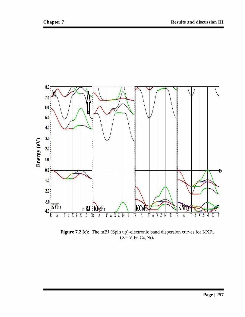
Chapter 7 Results and discussion ΙΙΙ
Page | 257
Figure 7.2 (c): The mBJ (Spin up)-electronic band dispersion curves for KXF3
(X= V,Fe,Co,Ni).
En
ergy
(eV
)
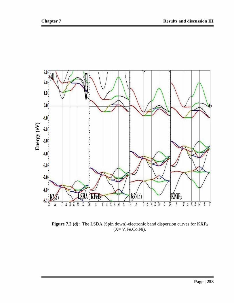
Chapter 7 Results and discussion ΙΙΙ
Page | 258
Figure 7.2 (d): The LSDA (Spin down)-electronic band dispersion curves for KXF3
(X= V,Fe,Co,Ni).
En
ergy
(eV
)

Chapter 7 Results and discussion ΙΙΙ
Page | 259
Figure 7.2 (e): The GGA (Spin down)-electronic band dispersion curves for KXF3
(X= V,Fe,Co,Ni).
En
ergy
(eV
)

Chapter 7 Results and discussion ΙΙΙ
Page | 260
Figure 7.2 (f): The mBj (Spin down)-electronic band dispersion curves for KXF3
(X= V,Fe,Co,Ni).
En
ergy
(eV
)

Chapter 7 Results and discussion ΙΙΙ
Page | 261
Energy (eV)
DO
S (
Sta
tes/
eV)
Figure 7.3: Spin-dependent total and partial density of states for (a) KVF3, (b) KFeF3,
(c) KCoF3 and (d) KNiF3.
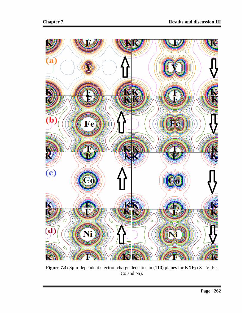
Chapter 7 Results and discussion ΙΙΙ
Page | 262
Figure 7.4: Spin-dependent electron charge densities in (110) planes for KXF3 (X= V, Fe,
Co and Ni).

Chapter 7 Results and discussion ΙΙΙ
Page | 263
Figure 7.5: The calculated imaginary part Ԑ2 (ω) of the dielectric function for KXF3
(X= V,Fe,Co,Ni) compounds.

Chapter 7 Results and discussion ΙΙΙ
Page | 264
Figure 7.6: The Calculated real part Ԑ1(ω) of the dielectric function for KXF3
(X= V,Fe,Co,Ni) compounds.

Chapter 7 Results and discussion ΙΙΙ
Page | 265
Figure 7.7: Calculated energy loss function L (ω) of the dielectric function for KXF3
(X= V,Fe,Co,Ni) compounds.
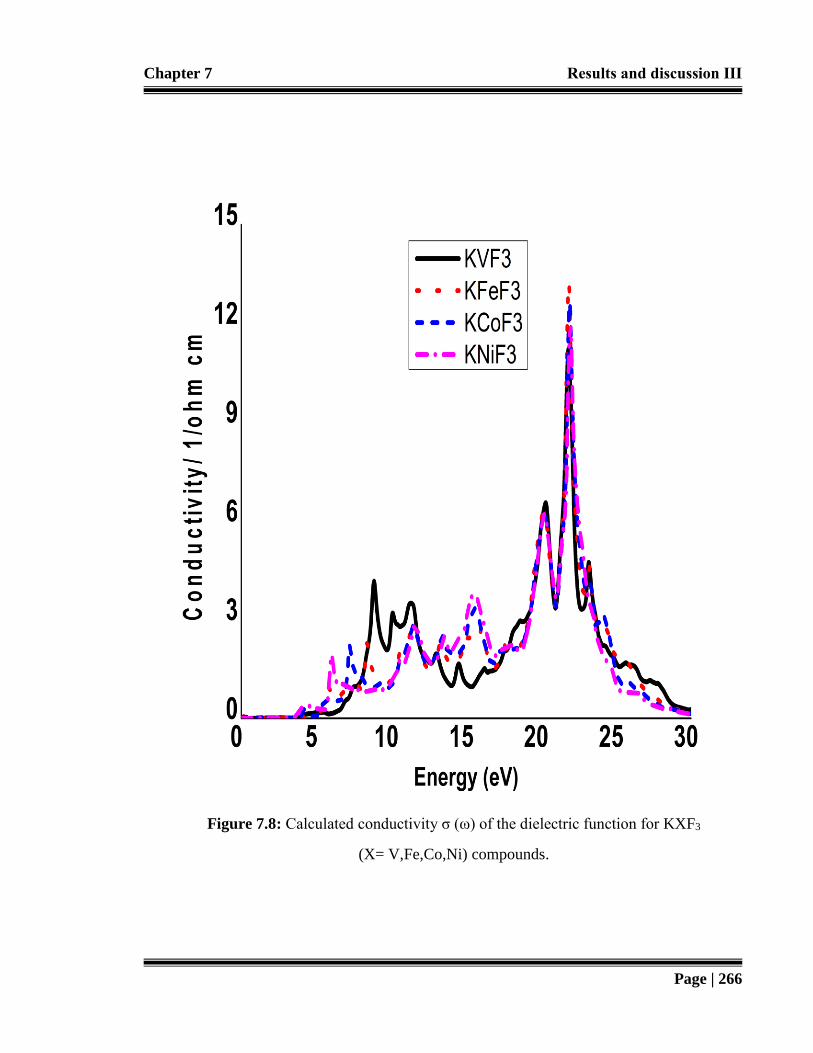
Chapter 7 Results and discussion ΙΙΙ
Page | 266
Figure 7.8: Calculated conductivity σ (ω) of the dielectric function for KXF3
(X= V,Fe,Co,Ni) compounds.

Chapter 7 Results and discussion ΙΙΙ
Page | 267
Figure 7.9: Calculated absorption coefficient α (ω) of the dielectric function for KXF3
(X= V,Fe,Co,Ni) compounds.

Chapter 7 Results and discussion ΙΙΙ
Page | 268
Figure 7.10: Calculated reflectivity R (ω) of the dielectric function for KXF3
(X= V,Fe,Co,Ni) compounds.
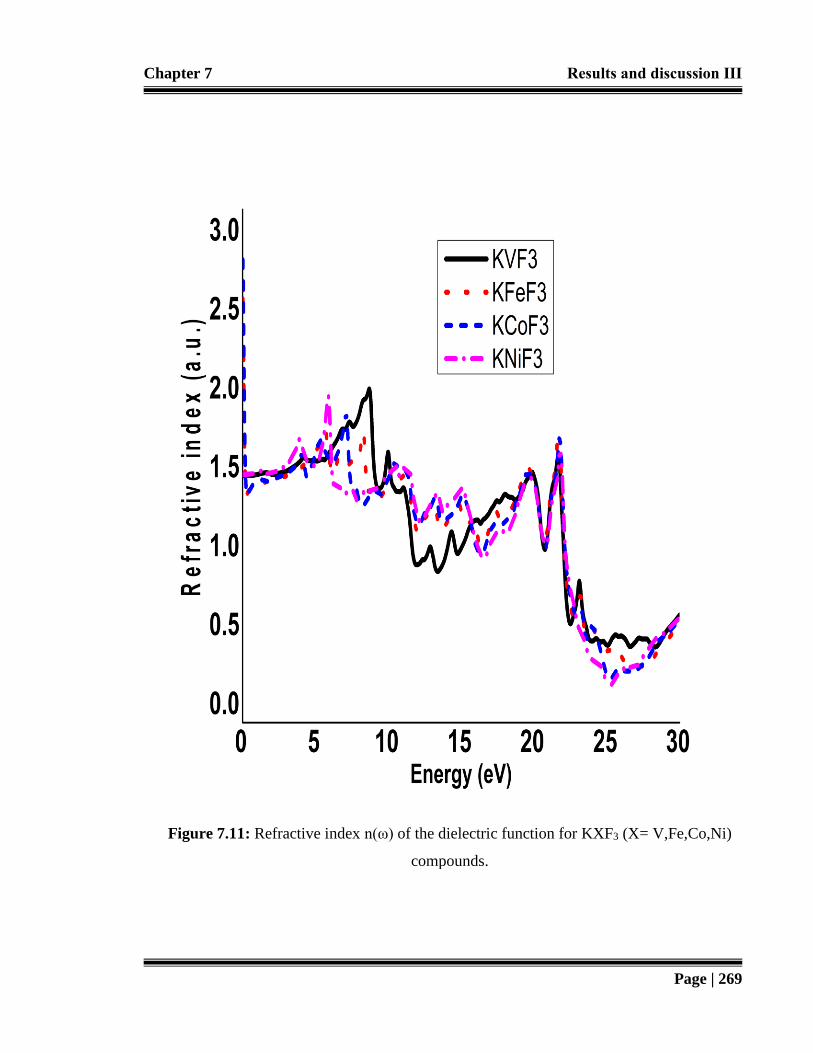
Chapter 7 Results and discussion ΙΙΙ
Page | 269
Figure 7.11: Refractive index n(ω) of the dielectric function for KXF3 (X= V,Fe,Co,Ni)
compounds.

Chapter 7 Results and discussion ΙΙΙ
Page | 270
Figure 7.12: Calculated sum rule (Neff) of the dielectric function for KXF3
(X= V,Fe,Co,Ni) compounds.

Chapter 7 Results and discussion ΙΙΙ
Page | 271
Table 7.1: Comparison of experimental and calculated values of equilibrium lattice constants
(ao in Ǻ), ground state energies (Eo in Ry), bulk modulus (Bo in GPa) and its pressure
derivative (BP), and bond lengths of KXF3 (X = V, Fe, Co,Ni) compounds.
a)(Moreira and Dias 2007), f)(Travis et al., 2016), g)(Lee et al., 2003), i)(Verma and Kumar 2012), k)(Shafer 1967)
(Experimental Work); b)(Jiang 2007), c)(Majeed 2010), d)(Verma et al., 2008),e) (Pari 1994),h) (Dovesi et al., 1997) (Other
theoretical work).
Compound Present work
——————— GGA
Present work
――—————
LDA
Present
Analytical work
——————— I.R method
Present
Analytical work
——————— V.J method
Experimental
work Other
theoretical
work
KVF3 ao (Å)
4.137 4.134 4.198 4.180 4.201a 4.134b,4.138c,
4.102c,3.847d Bo (GPa) 78.01 77.94 74.88e
BP(GPa) 4.95 Bond-lengths K-F(Å) 2.85 K-V(Å) 3.61 V-F(Å) 2.08 2.06f KFeF3 ao (Å)
4.064 4.059 4.089 4.042 4.130a,
4.129g
4.121c,4.124c,
4.120h,4.221i
Bo (GPa) 70.11 70.03 72.59e
BP(GPa) 3.68
Bond-lengths K-F(Å) 2.90 K-Fe(Å)
Fe-F(Å)
3.57
2.07 2.08f
KCoF3 ao (Å)
4.055 4.051 4.059 4.012 4.090i, 4.091a
4.092g
4.072b,4.076c
4.077d ,3.801d
Bo (GPa) 82.24 82.31 75.82e
BP(GPa) 4.89 5.06 Bond-lengths K-F(Å) 2.82 K-Co(Å) 3.47 Co-F(Å) 2.01 2.03k KNiF3 ao (Å)
4.018 4.013 4.117 4.110 4.020a,4.034g,
4.012f
4.015c,4.011c
Bo (GPa) 80.13 79.99 79.65e
BP(GPa) 5.05 Bond-lengths K-F(Å) 2.31 K-Ni(Å) 3.44 Ni-F(Å) 1.96 1.99f

Chapter 7 Results and discussion ΙΙΙ
Page | 272
Table 7.2: Calculated tolerance factor for KXF3 (X = V, Fe,Co,Ni) compounds.
a) (Travis et al., 2016), b) (Kocsis et al., 1999), c) (Moreira and Dias 2007)
Table 7.3: Calculated values of elastic constants (C11, C12 and C44 in GPa), for KXF3 (X =
V,Fe,Co,Ni) compounds.
a) (Aleksiejuk et al., 1975) (Experimental Work)
Tolerance
Factor Present work
——————————
Bond length formula
Present work
——————————
Goldschmidt’s formula
Experimental
work
Theoretical
work
KVF3 0.891 0.992 0.991a 0.997c
KFeF3 0.999 1.001 1.003b 1.002c
KCoF3 0.998 1.018 1.060b 1.019c
KNiF3 0.921 1.013 1.042a 1.047c
Sr.No. Parameters KVF3 KFeF3 KCoF3 KNiF3
1 C11 (GPa) 162.448 131.112 122.281
127.870a
121.231
2 C12 (GPa) 35.471 36.412 62.425
52.919a
58.989
3 C44 (GPa) 32.219 39.837 32.199
34.211a
46.639

Chapter 7 Results and discussion ΙΙΙ
Page | 273
Table 7.4: Calculated values of Bulk modulus (B0 in GPa), Young’s modulus (Y in GPa),
Voigt’s shear modulus (GV in GPa), Reuss’s shear modulus (GR in GPa), and Hill’s shear
modulus (GH in GPa) for KXF3 (X = V,Fe,Co,Ni) compounds.
a) (Verma and Kumar 2012) (Other theoretical work), b) (Dovesi et al., 1997) (Experimental Work)
Sr.No. Parameters KVF3 KFeF3 KCoF3 KNiF3
1 Bo(GPa) 77.798
74.889a
68.211
69.110b
82.377
75.828a
80.217
79.651b
2 Gv(GPa) 43.212 42.012 31.291 40.886
3 GR(GPa) 41.299 42.532 31.256 39.067
4 GH(GPa) 42.213 42.277 31.273 39.971
5 Y (GPa) 107.231 105.661 183.274 102.824

Chapter 7 Results and discussion ΙΙΙ
Page | 274
Table 7.5: Calculated values of B/G ratio, Shear constant (C’), Cauchy pressure (C’’),
Lame’s coefficients (λ and μ), Kleinman parameter (ξ in GPa), Anisotropy constant (A in
GPa) and Poisson’s ratio (ѵ in GPa) for KXF3 (X = V,Fe,Co,Ni) compounds.
Sr.No. Parameters KVF3 KFeF3 KCoF3 KNiF3
1 Bo/GH (GPa) 1.84 1.61 2.63 2.01
2 C′ 63.49 47.35 29.93 31.12
3 C′′ 3.26 -3.42 30.23 12.06
4 Ѵ (GPa) 0.27 0.24 0.31 0.29
5 A (GPa) 0.50 0.84 0.94 1.55
6 ξ(GPa) 0.37 0.43 0.63 0.64
7 λ 49.55 27.12 51.85 53.42
8 μ 42.22 42.23 31.78 39.97

Chapter 7 Results and discussion ΙΙΙ
Page | 275
Table 7.6: Comparison of experimental and calculated values of longitudinal (υl in Km/s),
transverse (υt in Km/s), average sound velocity (υm in Km/s), Debye temperature (θD in K)
and the melting temperature (TMelt in K) for KXF3 (X = V,Fe,Co,Ni) compounds.
Compound υl υt υm θD TMelt
KVF3
Present work
5.57 3.17 4.37 340 1500 ± 300
Experimental
work
1559a
KFeF3
Present work
5.37 3.13 4.25 325 1330 ± 300
Experimental
work
Other work
RbFeF3]1
4.95
2.59
340
1435b
1240 ± 300
KCoF3
Present work
5.49 2.75 4.12 312 1300 ± 300
Experimental
work
3.38c 247a 1305d
KNiF3
Present work
5.44 2.98 4.21 320 1225 ± 300
Experimental
work
Other work
RbNiF3]1
4.90
2.30
3.31c 262e
315
1400f
1173 ± 300
a) (Poirier 2000), b)(Hautier 2011), c) (Jong et al., 2015), d) (Holden 1971), e) Oleaga 2015, f)(Shafer et al., 1967)
(Experimental Work); 1) (Mubarak and Saleh 2015) (Other theoretical work)
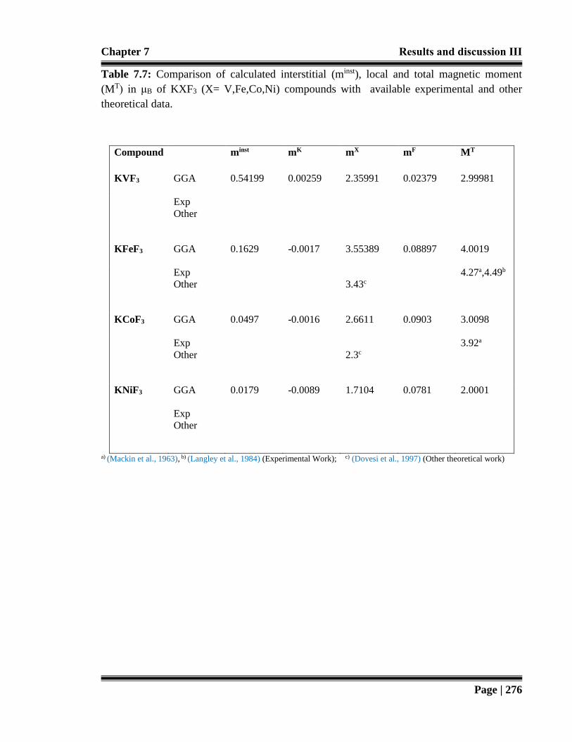
Chapter 7 Results and discussion ΙΙΙ
Page | 276
Table 7.7: Comparison of calculated interstitial (minst), local and total magnetic moment
(MT) in μB of KXF3 (X= V,Fe,Co,Ni) compounds with available experimental and other
theoretical data.
Compound minst mK mX mF MT
KVF3 GGA 0.54199 0.00259 2.35991 0.02379 2.99981
Exp
Other
KFeF3 GGA 0.1629 -0.0017 3.55389 0.08897 4.0019
Exp
Other
3.43c
4.27a,4.49b
KCoF3 GGA 0.0497 -0.0016 2.6611 0.0903 3.0098
Exp
Other
2.3c
3.92a
KNiF3 GGA 0.0179 -0.0089 1.7104 0.0781 2.0001
Exp
Other
a) (Mackin et al., 1963), b) (Langley et al., 1984) (Experimental Work); c) (Dovesi et al., 1997) (Other theoretical work)

Chapter 7 Results and discussion ΙΙΙ
Page | 277
7.8 Conclusion
In this chapter detailed theoretical investigation of four transition metal based
fluoroperovskites KXF3 (X= V,Fe,Co,Ni) have been done successfully. The electronic
structure calculations demonstrate prominent decrease in lattice constant as transition metal
in KXF3 changes from V to Ni, in accordance with the decrease in atomic size of the
corresponding compounds. These elastically and mechanically stable compounds reveal
dominant ductile behavior with high directional bonding. The calculations of Debye
temperature θD helps to explore significant thermal parameters for KXF3. The spin based
magneto-electronic characteristics clarifies the phenomenon of exchange splitting, is due to
3d states of transition metals. However, the optimized magnetic phase calculations validate
the experimental findings at low temperature. Furthermore, the linear optical response
confers wide extent of reflection as well as absorption within region of high frequency.
Hopefully this investigation, as per best of concerned knowledge, is benchmarked
investigation on KXF3 and this contribution helps to stimulate an outlook on these
fluoroperovskites in specified areas of interest. In light of effective magneto-opto-electronic
implications, KXF3 class of fluoroperovskites can be applicable in spin based switching
devices.

Chapter 8 Results and discussion ΙV
Page | 278
Chapter 8: Results and discussion ΙV;
Effect of pressure variation on strontium and calcium
based fluoroperovskites
“Never say, I tried it once
and it did not work.”
Ernest Rutherford
8.1 Introduction
The purpose of this chapter is to investigate detailed information about effect of pressure
variation on electronic structure, mechanical stability, opto-electronic trend and
thermodynamic aspects of strontium and calcium based alkali earth fluoroperovskites. This
chapter comprises of six major sections. Following the introduction section, the second
section comprises on back ground of materials, including significance for the effect of
hydrostatic pressure on physical properties. In section 8.3, effect of pressure variation on
detailed physical properties of SrLiF3 have been investigated. Section 8.4, is dedicated to
explore influence of pressure variation on structural, elastic, mechanical, opto-electronic and
thermodynamic parameters. In section 8.5, the effect of pressure variation on stability,
structural parameters, elastic constants, mechanical, electronic and thermodynamic properties
of cubic SrKF3 fluoroperovskite have been investigated by using the Full-Potential
Linearized Augmented Plane Wave (FP-LAPW) method combined with Quasi-harmonic
Debye model in which the phonon effects are considered. In section 8.6, Density functional
theory (DFT) is employed to calculate the effect of pressure variation on electronic structure,
elastic parameters, mechanical durability, and thermodynamic aspects of SrRbF3. The next

Chapter 8 Results and discussion ΙV
Page | 279
section 8.7, is used to calculate the effect of pressure variation (0-50 GPa) on electronic
structure, elastic parameters, mechanical durability, and thermodynamic aspects of calcium
based CaLiF3. At the end, the last section is dedicated to draw conclusion from the present
investigation.
8.2 Background of investigation
Perovskite fluorides with general stoichiometry ABF3, where A and B cations stands for
alkali and alkaline earth metals and F is a fluoride anion, gains considerable attention in the
last few decades due to their technological benefits. Generally, this diverse group of
fluoroperovskites are gaining potential utilization in the field of electric ceramics, optical
parametric oscillators, astrophysics, geophysics, heterogenous catalysis, refractories and so
on (Wang and Kang 1998). The importance of these fluoroperovskites are also hidden is their
technical applications such as solar energy convertors, low birefringent lenses, optical wave
guides, light emitting and spintronics devices (Tilley 2016). Therefore, the search of new
wide bandgap fluoroperovskite compounds for thermodynamic and opto-electronic
applications becomes necessary. Among them wide bandgap strontium and calcium based
fluoroperovskites such as “SrLiF3, SrNaF3, SrKF3, SrRbF3 and CaLiF3” has gained
prominent attention because some of them are prospective candidate for vacuum ultraviolet-
transparent lens materials in optical lithography and anti-reflective coatings (Mousa et al.,
2013).
Early experimental studies on SrLiF3 have mainly focused on its crystal structure such as
Düvel and its fellows (Düvel et al., 2011) analyzed BaLiF3 and SrLiF3 by Magic Angle
Spinning (MAS) Nuclear Magnetic Resonance (NMR) spectroscopy. They investigated that
SrLiF3 compound is a highly metastable quaternary fluoride crystallizes in inverse perovskite

Chapter 8 Results and discussion ΙV
Page | 280
structure. A comparative experimental study between SrLiF3 and BaLiF3 is also done by
Nishimatsu with his coresearchers (Nishimatsu et al., 2002). The authors found that SrLiF3
may have a wider and direct bandgap than BaLiF3. In another pressure induced study, Korba
with his fellows (Korba et al., 2009), have calculated opto-electronic properties of BaLiF3
under the influence of pressure and found that the valence bandwidth increases
monotonically with the pressure. Theoretically, there are few computational studies based on
common density functional theory approximations such as Local Density Approximation
(LDA) and Generalized Gradient Approximation (GGA) within first principles technique
(Yalcin et al., 2016; Mubarak 2014 & Mousa et al., 2013). Mubarak and Mousa (Mubarak
and Mousa 2012) performed first principles calculations of BaXF3 (X= Li,Na,K,Rb) fluoride
perovskites and found wide and direct (Γ-Γ) band gap in these compounds. While from
different optical spectra these compounds can be utilized in high frequency opto-electronic
application including transparent optical coatings. In chapter 5, section 5.2 and 5.3 (Erum
and Iqbal 2016 & Erum and Iqbal, March 2017), on SrMF3 (M= Li,Na,K,Rb), we explore
structural, elastic and optoelectronic response of these compounds under constant (zero)
pressure by using different exchange and correlation schemes. Our elastic and mechanical
properties prove mechanical stability, brittle, ionic nature in these compounds which can
utilize them in lens material manufacturing discipline because they would not tolerate major
birefringence which can make design of lenses difficult. While our results of optoelectronic
properties suggest implementation of these materials in UV based devices.
From previous studies, it can be evaluated that there are few theoretical and some
experimental investigation is devoted to study “SrLiF3, SrNaF3, SrKF3, SrRbF3 and CaLiF3”
compounds. Especially experimental work on them is scarce due to their reactive and volatile

Chapter 8 Results and discussion ΙV
Page | 281
nature and as per best of our knowledge neither experimental nor theoretical effort have been
made to investigate pressure dependent physical properties. Though pressure imposes
significant variation on important physical properties such as lattice parameters, electronic
density of states (DOS), band structure curves, elastic moduli, cubic stability conditions,
complex dielectric coefficients, refractive index, reflectivity and so on. Generally,
fluoroperovskites are made up of the network of corner linked polyhedral, tilt or distortion in
polyhedral upon application of temperature or pressure plays a crucial role in their stability
because change in pressure transfer electron from s state to p state imparts an important role
in the stability of crystal structure in cubic phase (Flocken et al., 1986). Motivation of this
study is to enhance the rare experimental and existing theoretical literature by investigating
effect of pressure variation on structural, elastic, mechanical, electronic, optical and
thermodynamic properties of above mentioned compounds. We are in hope that such
pressure induced investigation allows future researchers to improve stable utilization of
“SrLiF3, SrNaF3, SrKF3, SrRbF3 and CaLiF3” compounds in manufacturing practical devices.
In addition to it, especially thermodynamic properties are reported for the first time.
8.3 Pressure variation on physical properties of SrLiF3
In this section, the structural, electronic, elastic, optical and thermodynamic properties of
cubic fluoroperovskite SrLiF3 at ambient and high-pressure are investigated by using first-
principles total energy calculations (Murnaghan 1944) within the framework of Generalized
Gradient Approximation (GGA) (Wu and Cohen 2006), combined with Quasi-harmonic
Debye model (Schwarz et al., 2010), in which the phonon effects are considered. The
pressure effects are determined in the range of 0-50 GPa.

Chapter 8 Results and discussion ΙV
Page | 282
8.3.1 Pressure variation on structural properties
The structural properties are determined via different volumes over a range ± 10% which are
selected to calculate minimum ground state energy (Eo) at zero pressure. Here Birch
Murnaghan’s equation of state (EOS) (Murnaghan 1944) is used to fit the minimum energy
(Eo) versus minimum volume (VO). It can be noticed from Table 8.1 that calculated ground
state lattice parameters (at zero pressure) such as lattice constant of the present work is 3.871
Å, which is in good agreement with previously reported work in chapter 5 (Erum and Iqbal,
March 2017 & Erum and Iqbal 2016). However, between experimental (Castro 2002 &
Mishra et al., 2011) and present lattice parameter (ao) there is some deviation because the
present work is done at the ground state while the experimental work was done at ambient
conditions.
In order to examine the crystal structure of SrLiF3 on different hydrostatic pressure (0 to 50
GPa), we attempt to study the effect of different pressure, with a step size of 10 GPa, on
lattice parameters. Figure 8.1 depicts calculated change in the value of lattice constant by
LDA and GGA approximations. It can be interpreted that lattice constant is going to decrease
both by LDA and GGA approximations. The variation of bond lengths Sr-F and Li-F with
pressure is also presented in Figure 8.2. However, with comparison of data at constant
pressure of the same series as shown in Table 8.2 (Erum and Iqbal 2016), it can be analyzed
that Li-F and Sr-F bond lengths compress to a reasonable extent within the limit that
constituent polyhedral of SrLiF3 do not become distorted with the change in pressure. The
reduction in values of bond lengths and lattice constant can be associated via difference of
bandgap and hybridization strength which will be discussed in association with electronic
properties in upcoming section.

Chapter 8 Results and discussion ΙV
Page | 283
8.3.2 Pressure variation on electronic properties
The electronic properties at constant pressure (Zero pressure) are explored in terms of band
dispersion curves as well as electronic density of available states to occupy. Figure 8.3 and
Figure 8.4 illustrates that at constant compression SrLiF3 has both conduction band minima
(CBM) and valence band maxima (VBM) lies at direct (Γ- Γ) symmetry points resulting
7.306 eV bandgap from GGA approximation which as compared to previously reported
work, are in reasonable agreement as shown in Table 8.2.
The electronic nature of the herein investigated compound at constant pressure is also
confirmed by Density of States (Partial as well as Total) as shown in Figure 8.5. The
difference between F-2p states within 0 to -3 eV and Sr-4p states within -13 to -15 eV range
explores the transition of states at zero pressure. It can be interpreted that as a whole Sr-3d
peaks are dominant in conduction band energy region.
Next, we have discussed the effect of pressure applications of electronic properties of SrLiF3
fluoroperovskite. The key issue in SrLiF3 compound is formation and widening of bandgap
with the increase in pressure. It can be analyzed from Figure 8.3-8.5 that as compression
increases from 0 to 50 GPa, calculated bandgap increases from 7.306 eV to 7.782 eV from
GGA. It is worthy to mention here that in this pressure range the cubic structure remains
intact. The bandgap does not change its nature under application of pressure, although the
increase in bandgap of SrLiF3 at high pressure shifts towards wider gap nature and the rate of
increase of bandgap with pressure shows a plateau like behavior up to 50 GPa. In general, the
opening of wide band gap in the fluoroperovskites is because of electro-negativity of fluoride
ion (Harmel et al., 2015; Babu et al., 2014 & Mishra et al., 2011).

Chapter 8 Results and discussion ΙV
Page | 284
In this section, we try to summarize broadening of bandgap and reduction in lattice
parameters from several points of view. From DOS point of view, it can be observed that
upon compression an increase in the ratio of splitting between Sr-5d, Sr-4d, Sr-3d, F-2s and
F-2p states because the bands broadened the energy of Sr-4d and Sr-5d states, thereby
resulting an ultimate rise in the bandgap and this increase in bandgap continues up to 50 GPa.
Since Mishra with his coresearchers (Mishra et al., 2011) and Korba with his coresearchers
(Korba et al., 2009) have experimentally and theoretically confirmed the high-pressure
structural stability of BaLiF3 class of fluoroperovskites which is in accordance with our
results. As pressure is increased from 0 to 50 GPa, from lattice parameter point of view, the
cubic lattice nature of SrLiF3 compound remains stable, with reduced lattice constant (ao),
reduced bonds length and increased band gap. The similar nature of compression is also
observed by Lee and their fellows (Lee et al., 2004) as lessening in bonds length increases
the bond energy, which increases bandgap consequently, reduces the strength of covalent
bond. In some valuable theoretical (Murtaza and Iftikhar 2012) and experimental (Kuo et al.,
2004), studies, the similar inverse relation between lattice constant and bandgap is reported.
On the other hand, we also shed light to a prominent fact that LDA and GGA
approximations, undervalues bandgaps in wide bandgap insulators and semiconductors. The
reason of this underestimation lies in falsified clarification of factual unoccupied states as
compared to Khon–Sham states of the system (Wu and Cohen 2006). Here we highlight
modified Becke-Johnson potential (mBJ), to attain expected accurate results near to
experimental value, which is usually formed by well-known GGA and LDA calculations.
Furthermore, through mBJ scheme a bandgap near to experimental values is obtained like
Yalcin and his fellows (Yalcin et al., 2016) for BaLiF3, which predicts 8.2 eV bandgap by

Chapter 8 Results and discussion ΙV
Page | 285
mBJ potential (Tran and Blaha 2009), in similar accordance with experimental bandgap of
8.41 eV with just divergence of 1.78%. Similar trend is also observed for SrLiF3. As a result,
the cubic SrLiF3 is by virtue, an insulator and with the increase in the pressure the strength of
hybridization increases with reduced bond lengths which give rise to antibonding
phenomenon among bonds. This antibonding creates high energy, which pushed up energy
level away from Ef, consequently widening of bandgap occurs which is previously reported
in Pseudo potential theory (Imada et al., 1998 & Harrison 1984) as well.
8.3.3 Pressure variation on elastic properties
To verify structural constancy of SrLiF3 with compression 0-50 GPa, we reconnoiter
significant elastic and mechanical parameters. The variation of elastic responses under
compression can provide reliable information about change in stiffness, stability and
hardness of any compound. The complete pressure dependent mechanical behavior of any
crystals can be easily interpreted by its pressure dependent elastic properties. The major
importance of elastic constants is hidden in its response towards an applied macroscopic
stress (Meziani and Belkhir 2012). In this subsection, our main aim is to calculate elastic and
mechanical properties such as elastic constants, elastic modulus, elastic stiffness coefficients,
Poisson’s ratio (ѵ), Cauchy pressure (C''), Anisotropy constant (A), Kleinman parameter (ξ)
and Melting temperature (Tm) according to some detailed mathematical relationships as
mentioned in the following reference (Sadd 2005).
The basic idea used to calculate elastic coefficient for cubic crystals, (C11, C12, C44) is the
application of homogenous deformations with a finite value using first-principles
investigation (Jamal et al., 2014). The computation of stress tensor (ϭ) is done by using
Charpin method (Charpin 2001). By applying cubic symmetry, 21 independent components

Chapter 8 Results and discussion ΙV
Page | 286
of elastic constants are condensed to C11, C12, and C44 elastic constants. In the present work,
our results regarding to elastic and mechanical parameters are tabulated in Table 8.3-8.6.
Unfortunately, for comparison there is unavailability of data at higher pressure ranges but our
investigated results are in reasonable accordance with previous work on same series
compound such as on BaLiF3 (Mishra et al., 2011). The condition for mechanical stability
for cubic crystals (Wang et al., 1993) are found to be satisfied. Table 8.4 shows that the
calculated elastic constants, for cubic crystals under finite strain, obey the modified stability
criteria (erum and Iqbal, November 2017) according to corresponding pressure of 50 GPa.
i.e.
𝑀1 =(𝐶11+2𝐶12)
3+
𝑃
3> 0 (8.1)
𝑀2 = 𝐶44 − 𝑃 > 0 (8.2)
𝑀3 =(𝐶11− 𝐶12)
2− 𝑃 > 0 (8.3)
However, it can be noticed that at 50 GPa pressure the stability condition from equation 8.2
is not fully satisfied (At this pressure M2 stability criteria is lower than zero i.e. -0.53) as
shown in Figure 8.6. Therefore, the cubic fluoroperovskite SrLiF3 is mechanically stable
against elastic deformation by the compression up to 40 GPa. A monotonic linear
dependence is found for all pressure ranges, as shown in Figure 8.7-8.9. The elasticity in
length, C11, expand with pressure which means that pressure enhance tensile strength of
SrLiF3 compound. Similar trend for elasticity in shape is perceived for C44 elastic constant.
So, C11 and C44 increases, as a result of bond length enhancement (Sr-F, Li-F) which predicts
bonds length reduction.

Chapter 8 Results and discussion ΙV
Page | 287
8.3.4 Pressure variation on mechanical properties
The important mechanical aspects, as shown in Table 8.5, such as different form of shear
modulus G, can be calculated by using following expressions (Shafiq et al., 2015):
𝑮𝑽 = 𝟏
𝟓(𝑪𝟏𝟏 − 𝑪𝟏𝟐 + 𝟑𝑪𝟒𝟒) (8.4)
𝑮𝑹 =𝟓𝑪𝟒𝟒(𝑪𝟏𝟏−𝑪𝟏𝟐)
𝟒𝑪𝟒𝟒+𝟑(𝑪𝟏𝟏−𝑪𝟏𝟐) (8.5)
𝑮 =𝑮𝑽+𝑮𝑹
𝟐 (8.6)
However, expression of bulk modulus B are mention from following equation (Kittel 2005):
𝑩 =𝟏
𝟑 (𝑪𝟏𝟏 + 𝟐𝑪𝟏𝟐) (8.7)
The response of a material towards linear strain can be well defined by Young’s modulus via
following relation (Jenkins & Khanna 2005):
𝒚 =𝟗𝑩𝑮
(𝟑𝑩+𝑮) (8.8)
From the trend of Young’s modulus (Y), Bulk modulus (B0), Reuss’s shear modulus (GR),
Voigt’s shear modulus (GV), and Hill’s shear modulus (GH), it can be observed that SrLiF3
has highest value of stiffness and rigidity at pressure of 50 GPa and lowest value of stiffness
and rigidity at 0 GPa pressure which means that material becomes stiffer and less
compressible when applied pressure is increased. While the value of shear constant reveals
that ionicity in SrLiF3 increases as pressure varies from 0 to 50 GPa because ionic materials
have low values of shear constant as shown in Table 8.6. These results are in reasonable
accordance with the previous work related to perovskite compounds under the influence of
varying pressure by Rai and his fellows (Rai et al., 2014).
Next, by using Cauchy’s law or Cauchy pressure, the angular characteristics of atomic
bonding is elucidated. It can be well defined as follows (Brik 2011):

Chapter 8 Results and discussion ΙV
Page | 288
𝑪′′ = 𝑪𝟏𝟐 − 𝑪𝟒𝟒 (8.9)
If the value of this pressure is negative, then the material tends towards, directional bonding
and if the value is positive then the material is expected to be metallic in nature. The
investigated perovskite SrLiF3 have negative value of Cauchy pressure at 0 GPa pressure
which is going to shift towards positive value upon increasing pressure, but insulating nature
of SrLiF3 as BaLiF3 (Nishimatsu et al., 2002) at high pressure shows, changed sign of
Cauchy pressure is unbiased pointer of reduced angular characteristics of the atomic bonding
as shown in Table 8.6.
The ratio of compression to relative expansion can be expressed in terms of Poisson’s ratio,
as follows (Pettifor 1992):
ѵ =(𝟑𝑩−𝟐𝑮)
𝟐(𝟑𝑩+𝑮) (8.10)
The poisson’s ratio also agrees well with behavior of Cauchy pressure, indicating that
application of pressure reduces brittleness and angular bonding nature of SrLiF3 compound.
In manufacturing disciplines, elastic anisotropy parameter A plays an imperative character.
The relation can be well defined as follows (Jamal et al., 2016):
𝑨 =𝟐𝑪𝟒𝟒
(𝑪𝟏𝟏−𝑪𝟏𝟐) (8.11)
From the calculated value of elastic anisotropy factor, the degree of deviation of anisotropic
behavior can be determined. Another significant parameter which was introduced by
Kleinman, used to quantify material’s behavior towards bond stretching or bond bending; if
minimum bond stretching then Kleinman parameter ξ=1 but If compound possess minutest
value for bond bending then ξ=0 as (Kleinman 1962):
𝝃 =𝑪𝟏𝟏+𝟖𝑪𝟏𝟐
𝟕𝑪𝟏𝟏−𝟐𝑪𝟏𝟐 (8.12)
Chapter 8 Results and discussion ΙV
Page | 289
As pressure increases the value of Kleinman parameter shift towards higher values which
implies that compression induces low resistance against bond bending or bond angle
distortion, from the value of 0.4563 (0 GPa) to 0.4567 (50 GPa) respectively. To calculate
melting tendency of SrLiF3 compounds, the next task is to explore melting temperature,
above which material changes from its solid phase to its liquid phase (Fine et al., 1984):
Tm = 607 + 9.3B + 555 (8.13)
From the calculation of melting temperature, it can be assessed, that an increase in pressure
induces less tendency of melting extent of SrLiF3 and eventually increases its melting
temperature as shown in Figure 8.9 and Table 8.6 respectively.
8.3.5 Thermodynamic properties
In this section, thermodynamic properties are investigated for SrLiF3, within 0 to 600 K
temperature and 0 – 50 GPa pressure ranges, by means of the Quasi-harmonic Debye model
as implemented in the Gibbs program (Blanco et al., 2004 & Francisco et al., 1998). In this
model the vibrations of the crystal are treated as a continuum isotopic, obtained from the
derivatives of the total electronic energy volume.
8.3.5.1 The Quasi-harmonic Debye model
To study the thermodynamic properties of the SrLiF3 compound quasi-harmonic Debye
model is applied, in which the non-equilibrium Gibbs function can be written as (Rached et
al., 2009):
𝐺∗(𝑉; 𝑃; 𝑇) = 𝐸(𝑉) + 𝑃𝑉 + 𝐴𝑣𝑖𝑏[𝛳𝐷(𝑉); 𝑇] (8.14)
Where E (V) is the total energy per unit cell, PV corresponds to the constant hydrostatic
pressure condition, θD (V) is the Debye temperature, T is the absolute temperature and AVib is

Chapter 8 Results and discussion ΙV
Page | 290
the contribution of vibratory term, which can be written using the Debye model by the
density of state of the phonons as follows (Greiner et al., 1995):
𝐴𝑣𝑖𝑏(𝛳𝐷; 𝑇) = 𝑛𝑘𝑇 [9𝛳𝐷
8𝑇+ 3𝑙𝑛 (1 − 𝑒−
𝛳𝐷𝑇 ) − 𝐷 (
𝛳𝐷
𝑇)] (8.15)
Where n is the number of atoms per chemical formula, D (ϴD / T) is the Debye integral. For
an isotropic solid, θD can be expressed as (Anderson 1963 & Gibbs 1873):
𝛳𝐷 =ħ
𝑘[6𝜋2𝑉
1
2𝑛]
1
3√
𝐵𝑆
𝑀𝑓(𝜎) (8.16)
Where M is the molecular weight per unit cell; BS is the adiabatic bulk modulus, which in
Debye model, is generally equal isothermal bulk modulus BT in the Debye model, leading to
the following equation (Francisco et al., 2001):
𝐵𝑆 ≅ 𝐵𝑇 = 𝑉𝑑2 𝐸(𝑉)
𝑑𝑉2 (8.17)
where E is the total energy of the crystal at 0 K.
f (σ) is given in references (Bouhemadou et al., 2009) as:
𝑓(𝜎) = {3 [2 (21+ 𝜎
31−2𝜎)
3
2+ (
11+ 𝜎
31− 𝜎)
3
2]
−1
}
1
3
(8.18)
The Poisson coefficient is taken to be equal to 0.25 (Francisco et al., 1998).
A minimization of Gibbs function G* makes it possible to obtain the thermal equation of
state, the volume V (P, T) and the corresponding chemical potential G (P, T) as (Blanco et
al., 2004):
[𝜕𝐺∗(𝑉;𝑃;𝑇)
𝜕𝑉]
𝑃,𝑇= 0 (8.19)

Chapter 8 Results and discussion ΙV
Page | 291
By solving the equation (8.19) with respect to V, a thermal equation of state can be achieved
which can be used to deduce the macroscopic properties: the heat capacity at constant
volume CV, the entropy, and the coefficient of thermal expansion are given as follows
(Rached et al., 2009):
𝐶𝑉 = 3𝑛𝑘 [4𝐷 (𝛳
𝑇) −
3𝛳
𝑇
𝑒𝛳𝑇−1
] (8.20)
𝑆 = 𝑛𝑘 [4𝐷 (𝛳
𝑇) − 3𝑙𝑛 (1 − 𝑒−
𝛳
𝑇)] (8.21)
α = 𝛾𝐶𝑉
𝐵𝑇𝑉 (8.22)
Anharmonic effect of the vibrating lattice is usually described in terms of Gruneisen
parameter, γ defined by (Greiner et al., 1995):
𝛾 = − 𝑑𝑙𝑛𝛳(𝑉)
𝑑𝑙𝑛𝑉 (8.23)
The heat capacity at constant pressure, CP can be expressed as (Roza 2011):
𝐶𝑃 = 𝐶𝑉(1 + 𝛼𝛾𝑇) (8.24)
8.3.5.2 Pressure and temperature variation on thermodynamic properties
The thermodynamic properties of SrLiF3 within 0 to 600 K temperature and 0 – 50 GPa
pressure ranges, has been determined using the Quasi-harmonic Debye model in which the
Debye temperature depends only on the volume of the crystal. This method has been
implemented in the Gibbs code and uses Only a set of points {V, E (V)} calculated in the
equilibrium state for T = 0 and P = 0 (Blanco et al., 2004).

Chapter 8 Results and discussion ΙV
Page | 292
It can be noticed from Figure 8.10 (a-b) that at low temperatures heat capacities CV and CP
are proportional to T3, while at (T > 400K), CV tends to the Dulong-Petit limit (123.7 J mol-
1K-1), that is communal phenomenon in all solids at elevated temperatures, whereas CP
follows a linear increase (Ghebouli et al., 2012). The variation of the volume expansion
coefficient α(T) for the SrLiF3, is presented in Figure 8.10 (c). It can be observed that α
exhibits enhanced growth for low temperatures and then progressively inclines to rise
linearly at elevated temperatures. It should be distinguished that as the pressure increases, the
growth of α with the temperature becomes reduced. However, α decreases sharply with the
increase in pressure, for a given temperature.
The Debye cut-off frequency or Debye temperature (θD) is a significant form of temperature,
have used to quantify several thermodynamic properties in the solid. It is important due to
extraction of some useful physical quantities for example specific heat capacities and melting
point. (Anderson 1963). It can be perceived from Figure 8.10 (d) that θD is almost continual
since 0 to 100 K, then declines smoothly with the temperature for T > 200K. While the
Debye temperature increases linearly with pressure, for a constant temperature. At zero
pressure and ambient temperature, the calculated θD is 511.62 K.
8.3.6 Pressure variation on optical properties
One of the most significant property to discuss internal structure of any material is optical
property. These properties suggest material’s suitability and reliability in industrial
applications, specifically for opto-electronics (Erum and Iqbal, December 2017). The set of
complete optical properties such as complex dielectric function Ԑ(ω), absorption coefficient
α(w), refractive index n (ω) and reflectivity R (ω), optical conductivity σ(ω), energy loss
function L(ω), and effective number of electrons neff via sum rules are calculated within

Chapter 8 Results and discussion ΙV
Page | 293
pressure 0-50 GPa. All optical parameters which are calculated here, are based on some
proposed numerical relations. The real and imaginary part of dielectric function Ԑ(ω) can be
defined as follows (Wooten 1972):
Ԑ(𝜔) = Ԑ1(𝜔) + 𝑖Ԑ2(𝜔) (8.25)
In equation (8.25) Ԑ1(ω) and Ԑ2(ω) represents real and imaginary part of dielectric function
respectively. The imaginary part of dielectric function Ԑ2(ω) can be given as:
Ԑ2(𝜔) = (4𝜋2𝑒2
𝑚2𝜔2) ∑ ∫ ⟨𝑖|𝑀|𝑗⟩2𝑓𝑖(1 − 𝑓𝑖)𝛿(𝐸ј,𝑘 − 𝐸𝑖,𝑘 − 𝜔)
𝑘𝑖,𝑗 𝑑3𝑘 (8.26)
As shown in Figure 8.11 (a), the interpretation of imaginary part of dielectric function plot,
describes complete response of material due to applied electromagnetic field which is
influenced by intraband as well as interband transitions (Monkhorst and Pack 1976). It can
be noticed that at zero pressure the threshold point is at about 7.306 eV which is critical point
in band gap edge of the SrLiF3 compound also known as fundamental absorption edge.
However, by increasing pressure from 0 to 50 GPa, the fundamental absorption edge shift
towards higher energy. This shift of threshold point is due to increase in bandgap (as detailed
explanation is mentioned in electronic property section). The main cause of this shift is
transition of electrons from valence band maxima to conduction band minima in SrLiF3
compound. These peaks positioned just below the zero energy Fermi level (EF), are ascribed
to transitions of F-2p state along with minor contribution of Sr-3d and Li-states. However,
within pressure range 0-50 GPa, this compound work well in ultraviolet region of
electromagnetic spectrum because of larger value of band gap than 3.1 eV (Murtaza and
Iftikhar 2012). Next, the real part of dielectric function Ԑ1(ω) is given by the well-known
Kramers-Kronig relation via corresponding equation (Abelès 1972):
Chapter 8 Results and discussion ΙV
Page | 294
Ԑ1(𝜔) = 1 +2
𝜋𝑃 ∫
ὠԐ2(ὠ)𝑑ὠ
ὠ2−ὠ2
ⱷ
0 (8.27)
It describes Ԑ1(ω) defines electric polarizability and absorptive behavior of the material. The
calculated plot of real dielectric function Ԑ1(ω) is displayed in Figure 8.11 (b). Ԑ1(0) has value
of about 2.12 for 0.00 GPa pressure and is found to be increased with increasing pressure
while at 50 GPa, the value of Ԑ1(0) reaches up to 2.38. This trend in pressure variation study
reveal the inverse behavior of Ԑ1(0) with electronic band gap, which has also been observed
for other fluoroperovskites (Harmel et al., 2015 & Babu et al., 2014).
The calculated values of complex dielectric function Ԑ(ω) can allow to determine key optical
function for the electromagnetic spectrum such as refractive index n(ω), reflectivity R,
optical conductivity σ(ω), and electron energy loss spectrum L(ω) which can be determined
by following expressions (Fox 2001):
𝑛(𝜔) = 1
√2[√Є1(𝜔)2 + Є2(𝜔)2 + Є1(𝜔) ]
1
2 (8.28)
𝑅 = |𝑛−1
𝑛+1|
2
(8.29)
𝜎(𝜔) = 2𝑊𝐶𝑉ℏ𝜔
𝐸02 (8.30)
𝐿(𝜔) = 𝐼𝑚 (−1
Ԑ(𝜔)) (8.31)
The calculated n(ω) plot from Figure 8.11(c) have similar shape as of Ԑ1(ω) curve. While
peaks shift towards higher energies which suggests higher values of refractive index which is
beneficial for successful utilization of this material in photonic applications. The computed
value of zero frequency reflectivity is 0.035, which can be clearly observed from Figure
8.11(d) that pressure encounter broadening of the maximum reflectivity range, in accordance

Chapter 8 Results and discussion ΙV
Page | 295
with the trend of Ԑ1(0). Our calculated value of optical conductivity σ(ω) for SrLiF3
compound is shown in Figure 8.11(e) The figure reveals that optical conduction at zero
pressure starts at approximately, 5eV originating after minor rising crests then finally shifts
towards higher energy ranges as pressure is increased and gains maximum peaks within
energy range of 12-14 eV. It is obvious as of this investigation that optical conductivity
spectrum swings near to increased energy ranges from 0 to 50 GPa due to increased bandgap
with pressure and this abrupt increase in conduction is due to trailing edge of Ԑ1(ω) curve. A
similar trend of behavior like optical conductivity is detected for coefficient of absorption
α(w), as portrayed in Figure 8.11(f). The energy loss function per moving electron is shown
in Figure 8.11(g) via energy loss function L(w). These peaks give us brief characteristics
related to phenomenon of plasma resonance. It can be observed that no energy loss occurs for
photon energy less than at about 7 eV for 0-50 GPa pressure but as soon as the photons
exceeds from this limit, the energy loss will start increasing and get maximum peaks.
However, it can be clearly seen from Figure 8.11(g) that pressure shifts energy loss function
towards higher energy region.
In the end, the sum rule is evaluated to consider the number of effective valence electrons via
corresponding formula (Abelès 1972):
𝑛𝑒𝑓𝑓(𝜔) = ∫ 𝜎(ὠ)𝜔
0ὠ 𝑑ὠ (8.32)
As shown in Figure 8.11(h), for SrLiF3 compound explored that electrons at zero pressure
initiates interband transitions about 5.5 eV. These peaks intensify gradually but at about 14-
16 eV range, rapid increase in saturation ratio of electrons can be observed. So, it can be
concluded that with the increase in pressure, the peaks move towards higher energies so the
number of effective electrons taking part in intraband as well as interband transitions

Chapter 8 Results and discussion ΙV
Page | 296
decrease. To best of our information there is lack of investigated information on pressure
dependent optical behavior of SrLiF3 in cubic phases we therefore hope that our work
provides better beneficial understanding about pressure dependent behavior of this material.
So, it can be concluded that with the increase in pressure, the peaks move towards higher
energies so the number of effective electrons taking part in intraband as well as interband
transitions decrease.
To best of our information there is lack of investigated information on pressure dependent
physical behavior of SrLiF3 in cubic phases so hopefully this work will motivate research
scholars to done theoretical as well as experimental studies in this direction, so they can
compare their results with our work to get better beneficial understanding about pressure
dependent behavior of this material.

Chapter 8 Results and discussion ΙV
Page | 297
Figure 8.1: The Pressure variation of Lattice Constant (a) GGA (b) LDA
Figure 8.2: The Pressure variation of Bonds length (a) Sr-F (b) Li-F

Chapter 8 Results and discussion ΙV
Page | 298
Figure 8.3: The Pressure dependence of Band Gap (a) GGA (b) mBj

Chapter 8 Results and discussion ΙV
Page | 299
Figure 8.4: The electronic band structures of SrLiF3 under the application of pressure
(0, 10, 20, 30, 40 and 50 GPa) calculated using GGA Approximation.
En
ergy
(eV
)

Chapter 8 Results and discussion ΙV
Page | 300
Figure 8.5: The Total and Partial Density of states (TDOS & PDOS) of SrLiF3 at 0 GPa
using GGA Approximation.
Energy (eV)
DO
S (
Sta
tes/e
V)

Chapter 8 Results and discussion ΙV
Page | 301
Figure 8.6: Stability criteria for cubic SrLiF3 compound as a function of
pressure.
Figure 8.7: Calculated pressure dependence of elastic constant/moduli
(a) C11 (b) C12 for SrLiF3 compound.

Chapter 8 Results and discussion ΙV
Page | 302
Figure 8.8: Calculated pressure dependence of (a) Elastic constant/moduli (C44)
(b) Bulk modulus (B) for SrLiF3 compound.
Figure 8.9: Calculated pressure dependence of Kleinman parameter (ξ), and
Melting temperature (Tm) for SrLiF3 compound.

Chapter 8 Results and discussion ΙV
Page | 303
Figure 8.10 (a): Variation of the specific heat capacities (Cp) versus temperature at
different pressures for SrLiF3 compound.
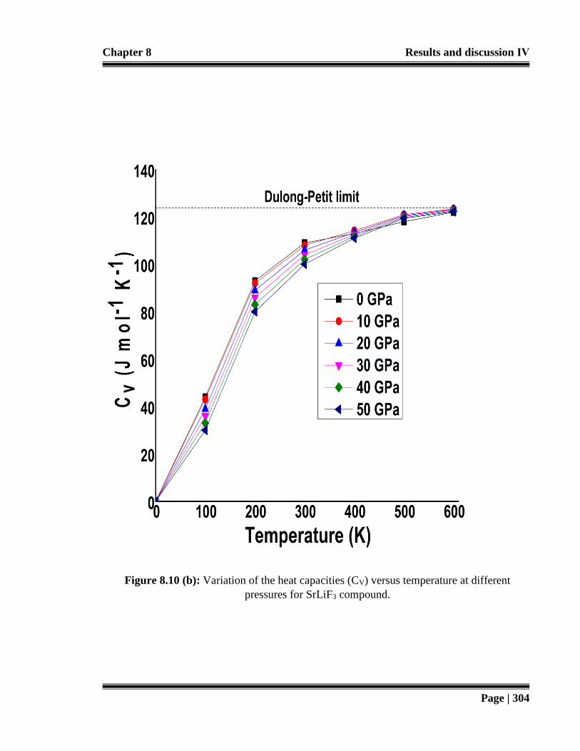
Chapter 8 Results and discussion ΙV
Page | 304
Figure 8.10 (b): Variation of the heat capacities (CV) versus temperature at different
pressures for SrLiF3 compound.

Chapter 8 Results and discussion ΙV
Page | 305
Figure 8.10 (c): Temperature dependence of the volume expansion coefficient α(T) at
different pressures for SrLiF3 compound.

Chapter 8 Results and discussion ΙV
Page | 306
Figure 8.10 (d): Variation of the Debye temperature (θD) as a function of temperature at
different pressures for SrLiF3 compound.

Chapter 8 Results and discussion ΙV
Page | 307
Figure 8.11 (a): Calculated Imaginary part Ԑ2 (ω) of the dielectric function as a function of
pressure for SrLiF3 compound.

Chapter 8 Results and discussion ΙV
Page | 308
Figure 8.11 (b): Calculated Real part Ԑ1 (ω) of the dielectric function as a function of
pressure for SrLiF3 compound.

Chapter 8 Results and discussion ΙV
Page | 309
Figure 8.11 (c): Calculated Refractive index n (ω) as a function of pressure for SrLiF3
compound.

Chapter 8 Results and discussion ΙV
Page | 310
Figure 8.11 (d): Calculated Reflectivity R(ω) as a function of pressure for SrLiF3 compound.

Chapter 8 Results and discussion ΙV
Page | 311
Figure 8.11 (e): Calculated Conductivity σ (ω) as a function of pressure for SrLiF3
compound.

Chapter 8 Results and discussion ΙV
Page | 312
Figure 8.11 (f): Calculated Absorption coefficient α (w) as a function of pressure for SrLiF3
compound.
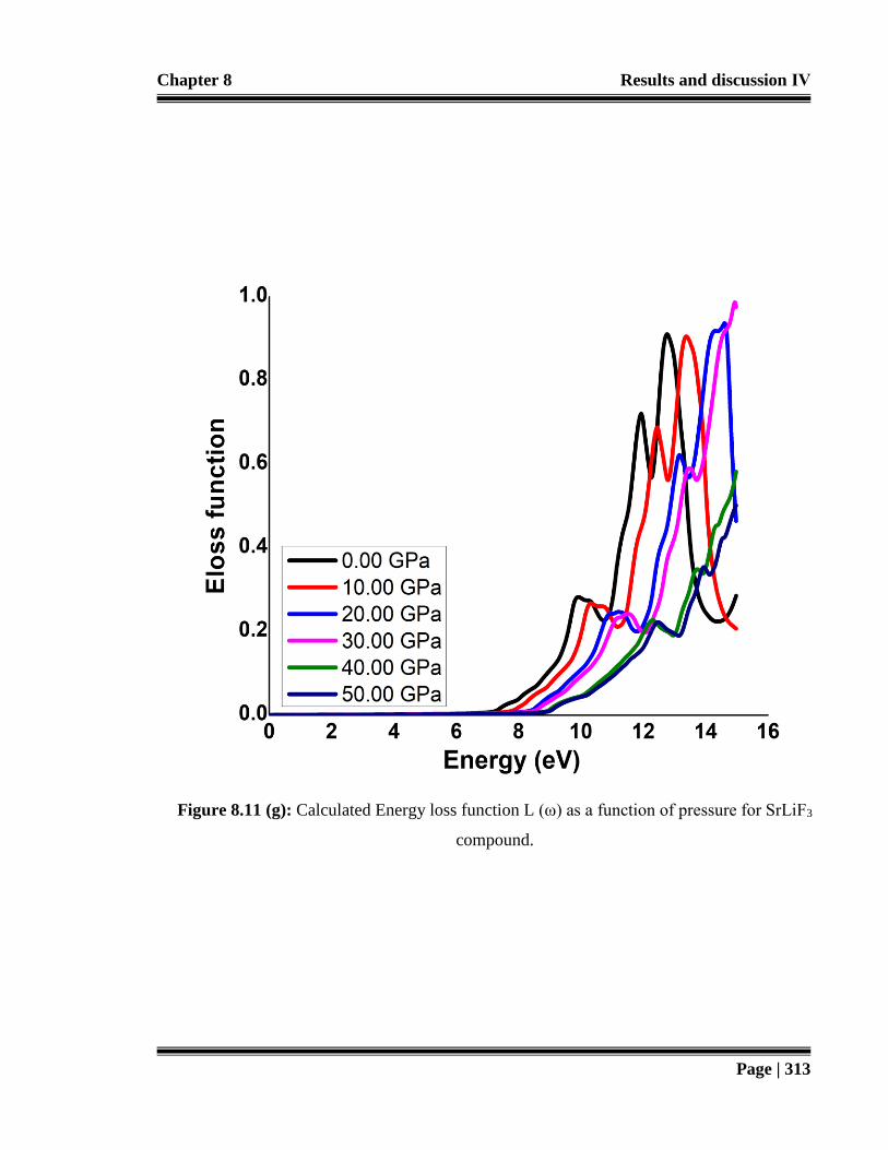
Chapter 8 Results and discussion ΙV
Page | 313
Figure 8.11 (g): Calculated Energy loss function L (ω) as a function of pressure for SrLiF3
compound.

Chapter 8 Results and discussion ΙV
Page | 314
.
Figure 8.11 (h): Calculated Sum rule as a function of pressure for SrLiF3 compound.

Chapter 8 Results and discussion ΙV
Page | 315
Table 8.1: Comparison of the present calculation with the previous experimental and
theoretical values for the lattice constants (ao), ground state energies (Eo), bulk modulus (Bo)
and its pressure derivative (B′) at ambient pressure of SrLiF3 compound.
Compound: SrLiF3 Present work
Experimental work/ Other work
ao (Å) 3.871 4.449a/ 3.879c, 3.871d, 3.762e, 3.754 f
Bo (GPa) 72.055 72.071 b/72.861c, 71.350 d
B′ (GPa) 4.353 4.356e
a) (Castro 2002), b) (Mishra et al., 2011) (Experimental Work) c) (Mousa et al., 2013), d) (Mubarak and Mousa
2012),e) (Erum and Iqbal 2016 & Erum and Iqbal, March 2017) (Other theoretical work)
Table 8.2: Comparison of previous and calculated values of Pressure (P in GPa), Energies (E
in Ry), Volume of unit cell (V in (a.u.)3), Energy Gap (eV), and Bond length (dSr-F, dLi-F).
a) (Mubarak and Mousa 2012) b) (Sarukura et al., 2007), c) (Nishimatsu et al., 2002), d) (Erum and Iqbal 2016),
e) (Erum and Iqbal, March 2017)
Pressure
(GPa)
Energies
(Ry)
Volume
(a.u.)3
Energy Gap (eV) dSr-F
(Ǻ)
dLi-F
(Ǻ)
dX-F (Ǻ) (X=
Li,Na,K,Rb)d Present (GGA)
Present (mBJ)
Previous (0.00 GPa)
0 -6974.891 394.1935664 7.306 9.201 7.21a(GGA)
2.521 1.849 dSr-F = 2.52
(0.00 GPa)
10 -6974.863 353.0442656 7.455 9.337 7.30b(GGA) 2.517 1.843 dLi-F = 1.85
(0.00 GPa)
20 -6974.855 328.1655202 7.591 9.411 7.19c(GGA) 2.511 1.838 dNa-F = 2.23
(0.00 GPa)
30 -6974.839 367.3939371 7.646 9.463 7.28d(GGA) 2.508 1.833 dK-F = 2.60
(0.00 GPa)
40 -6974.812 409.6302366 7.768 9.524 9.20e(mBj) 2.501 1.828 dRb-F = 2.74
(0.00 GPa)
50 -6974.798 454.9855278 7.782 9.501 2.503 1.830

Chapter 8 Results and discussion ΙV
Page | 316
Table 8.3: Calculated values of elastic constants (C11, C12, C44) of SrLiF3 at pressure from 0-
50 GPa.
a) (Erum and Iqbal 2016), b) (Mishra et al., 2011)
Table 8.4: Derived elastic constants characterizing mechanical stability (Equations 8.1-8.3)
of SrLiF3 at pressure from 0-50 GPa.
Pressure (GPa) M1 M2 M3
0
BaLiF3] a
75.48
73.90
49.45
47.13
57.19
46.79
10 78.82 39.45 47.19
20 82.16 29.45 37.19
30 85.49 19.46 27.19
40 88.83 9.46 17.20
50 92.16 -0.53 7.20
a) (Mishra et al., 2011)
Pressure
(GPa)
0 10 20 30 40 50 Previous
Work
(0.00 GPa)
C11 (GPa) 151.741 151.750 151.758 151.765 151.771 151.780 151.7a, 154.2b
C12 (GPa) 37.353 37.365 37.372 37.386 37.395 37.404 37.3a, 38.5b
C44 (GPa) 49.447 49.455 49.466 49.478 49.489 49.496 49.4a, 48.1b

Chapter 8 Results and discussion ΙV
Page | 317
Table 8.5: Calculated values of elastic moduli Bulk modulus (B0), Voigt’s shear modulus
(GV), Reuss’s shear modulus (GR) and Hill’s shear modulus (GH), and Young’s modulus (Y)
of SrLiF3 at pressure from 0-50 GPa.
a) (Erum and Iqbal 2016), b) (Mubarak and Mousa 2012), c) (Mishra et al., 2011)
Table 8.6: Calculated values of Shear constant (C’), Cauchy pressure (C’’), Poisson’s ratio
(ѵ) Anisotropy constant (A), Kleinman parameter (ξ), and melting temperature (Tm) of
SrLiF3 at pressure from 0-50 GPa.
a) (Erum and Iqbal 2016), b) (Mishra et al., 2011)
Pressure
(GPa)
0 10 20 30 40 50 Previous
Work (0.00
GPa)
Bo(GPa) 74.481 74.489 74.495 74.504 74.513 74.524 74.4a 72.2b
Gv(GPa) 52.546 52.550 52.557 52.563 52.569 52.573 52.5a,
GR(GPa) 52.280 52.284 52.292 52.299 52.306 52.310 52.281
GH(GPa) 52.413 52.417 52.424 52.431 52.437 52.442 52.4a, 52.2c
Y(GPa) 127.363 127.374 127.390 127.406 127.421 127.434 127.362 a
Pressure (GPa) 0 10 20 30 40 50 Previous
Work (0.00
GPa)
C' 57.194 57.193 57.193 57.190 57.188 57.188 57.194a
C'' -12.094 -12.090 -12.088 -12.085 -12.081 -12.079 -12.094a
Ѵ (GPa) 0.2151 0.2163 0.2174 0.2172 0.2184 0.2187 0.2150a
A (GPa) 0.8645 0.8647 0.8649 0.8652 0.8654 0.8655 0.86a, 0.83b
ξ(GPa) 0.4563 0.4564 0.4564 0.4565 0.4566 0.4567 0.4563a
Tm(K) 1854.67 1854.75 1854.80 1854.89 1854.97 1855.07 1854.65a

Chapter 8 Results and discussion ΙV
Page | 318
8.4 Effect of pressure variation on physical properties of SrNaF3
In this section, the effect of pressure variation on structural, electronic, elastic, mechanical,
optical and thermodynamic characteristics of cubic SrNaF3 fluoroperovskite have been
investigated by employing first-principles method. For the total energy calculations, the Full-
Potential Linearized Augmented Plane Wave (FP-LAPW) method (Schwarz et al., 2010) is
employed. Thermodynamic properties are computed in terms of Quasi-harmonic Debye
model (Blanco et al., 2004), within 0-25 GPa pressure and 0-600 K temperature.
8.4.1 Pressure variation on structural properties
The herein investigated compound SrNaF3 crystallize itself in ideal cubic perovskite structure
with space group Pm-3m (no. 221). The details of various lattice parameters, tolerance factor,
bond lengths, bulk modulus, and its pressure derivative at zero pressure are previously
reported in chapter 5 (Erum and Iqbal, March 2017 & Erum and Iqbal 2016). However, for
the continuation of thesis, brief form of previously calculated lattice parameters is mentioned
in Table 8.7, at constant (zero) pressure. The main aim of this section is to explore the
influence of external pressure on the electronic structure of SrNaF3 fluoroperovskite. Here
we examine effect of pressure variation in the range of 0-25 GPa with a step size of 5 GPa. It
can be observed from Figure 8.12 that calculated lattice constants by LDA and GGA
approximations are going to decrease under the influence of increase in pressure while the
calculated change in bond lengths Sr-F and Na-F under the effect of increasing pressure is
shown in Figure 8.13. It can be noticed from Table 8.8, that bond lengths are also going to
decrease as pressure is increased. As compared to our previous work / other work (Erum and
Iqbal, March 2017 & Erum and Iqbal 2016; Düvel et al., 2011 & Korba et al., 2009) (at
Chapter 8 Results and discussion ΙV
Page | 319
fixed pressure), it can be evaluated, that lattice constants, bond lengths and volume of unit
cell compress to a reasonable extent. As a result, the constituent polyhedral of SrNaF3 do not
become distorted by the change in pressure from 0-25 GPa. However, in the next section we
discuss the reason of this decrease via lattice associated parameters in conjunction with
electronic band structure and density of states (DOS).
8.4.2 Pressure variation on electronic properties
The concept of electronic nature of SrNaF3 are discussed in terms of Density of States, Total
as well as Partial (TDOS & PDOS) and electronic band structure calculations are figured out
in Figure 8.14-8.16. At zero pressure, SrNaF3 has a direct energy bandgap with the valence
band maxima (VBM) and conduction band minima (CBM) both located at the Γ symmetry
point resulting wide and direct (Γ- Γ) bandgap of 5.551 eV from GGA approximation while
from TB-mBj functional larger bandgaps of 8.298 eV is observed as shown in Table 8.8 and
in Figure 8.14-8.15. This change in the value of bandgap is in continuation with previous
study (Erum and Iqbal, March 2017 & Yalcin et al., 2016), that GGA and LDA schemes
undervalues energy bandgap of wide bandgap semiconductors and insulators. The cause of
this underestimation is discussed in detail by Tran and Blaha (Tran and Blaha 2009 & Grabo
et al., 1997). The Total and Partial Density of States (TDOS & PDOS) occupies energy
interval from (EF - 25 eV) up to (EF + 15 eV) at 0 GPa and 25 GPa pressure ranges as shown
in Figure 8.16. It can be observed that above fermi level slightly wide peak is dominated by
Sr-3d state at about (EF + 8 eV). Next energy interval (EF - 3 eV) is governed by F-2p state.
The upper valence band situated in a range from (EF - 12 eV) to (EF - 25 eV) is due to
hybridized state between Sr-4p, Na-2p and F-2s states respectively. Next, we have discussed
influence of increase in pressure from (0-25 GPa) range, (below which compound remains

Chapter 8 Results and discussion ΙV
Page | 320
stable in cubic phase) in terms of electronic band structure. The motivating fact of SrNaF3
compound is formation and widening of bandgap by the increase in pressure, illustrating
potential application of this compound in modern opto-electronic devices. The variation of
energy gap as a function of pressure are shown in Figure 8.14 and Figure 8.15. It can be
clearly observed that as the value of compression increases from 0 to 25 GPa, calculated
bandgap energy increase from 5.551 eV to 7.063 eV. It is worthy to mention here that
bandgap does not change its nature under pressure, although conduction band at Γ symmetry
point of Brillouin Zone shift towards higher energy ranges. However, the rate of widening of
bandgap with the increase in pressure shows a plateau like behavior up to 25 GPa. In general,
the widening of bandgap in fluorine based perovskites are due to the dominant
electronegative influence of fluoride ion (Harmel et al., 2015; Babu et al., 2014 & Mishra et
al., 2011).
The important issue to discuss here is that, what is the reason behind broadening of bandgap
and reduction in lattice parameters. In view of lattice parameter with the increase in pressure
from 0 to 25 GPa, there is attributed decrease in nearest neighbor distance, and in bond
lengths as well. The inverse relation between above mentioned parameters and bandgap is
already reported experimentally (Mishra et al., 2011) and theoretically (Korba et al., 2009).
Another similar behavior of compression is also observed by Lee and their fellows (Lee et
al., 2004) as decrease in bond lengths increases the bond energy, which reduces the strength
of covalent bond, consequently a wider bandgap. In fact, broadening of band energy upon
compression is due to broadened energy of Sr (4d & 5d) states which increases the ratio of
splitting between Sr-3d, Sr-4d, Sr-5d, F-2s and F-2p states respectively. This shift ultimately
moves bandgap towards higher energies and this increase in bandgap continues up to 25 GPa.

Chapter 8 Results and discussion ΙV
Page | 321
Since Mishra with his coresearchers (Mishra et al., 2011) and Korba with his coresearchers
(Korba et al., 2009) have experimentally and theoretically confirmed the high-pressure
structural stability which is in suitable accordance with band structures and DOS results. As a
result, with the increase in pressure of SrNaF3 the strength of hybridization increases with
reduced bond length which give rise to antibonding phenomenon among bonds. This
antibonding creates high energy, which pushed up energy level away from EF, consequently
widening of bandgap occurs which is previously reported in Pseudo potential theory (Imada
et al., 1998 & Harrison 1984) as well.
8.4.3 Pressure variation on elastic and mechanical properties
In order to verify structural, mechanical and cubic stability of SrNaF3 fluoroperovskite, we
shed light on the pressure dependence within range 0-25 GPa of the significant elastic and
mechanical parameters. To study the change in behavior of elastic properties, we performed
calculations at several values of reduced volumes, each of which corresponds to the system at
fixed hydrostatic pressure up to 25 GPa with the step size of 5 GPa. This is done by
performing complete optimization against each pressure value. Furthermore, the
computation of stress tensor (ϭ) is done with the help of Charpin method (Charpin 2001), by
applying cubic symmetry to 21 independent components of elastic constants which are
condensed to C11, C12, and C44 elastic constants respectively. The variation of elastic
constants under pressure gives reliable information regarding to change in stability, stiffness
and hardness of SrNaF3 compound. Here we calculate elastic and mechanical properties such
as elastic constants, elastic modulus, elastic stiffness coefficients, according to some
proposed mathematical relationships as mentioned in section 8.3.3-8.3.4. The complete list of
calculated elastic and mechanical parameters under compression are tabulated in Table 8.9-
Chapter 8 Results and discussion ΙV
Page | 322
8.11. Unluckily for SrNaF3, there is lack of availability for data to compare at high pressure
ranges so we only compare data of relevant compounds at zero pressure, which are found to
be in good agreement (Erum and Iqbal, March 2017 & Erum and Iqbal 2016; Düvel et al.,
2011 & Korba et al., 2009). Hence these results can serve as a reference for future
investigations.
A monotonic linear dependence of all curves of elastic constant/moduli can be observed from
Figure 8.17 and Table 8.9-8.10. The elastic constant, C11 which is related to longitudinal
distortion, linearly increases as with the change in pressure from 145.490 GPa to 429.043
GPa from 0 to 25 GPa. This is due to the fact that C11 increases as a result of bond strength
enhancement between Sr-F and Na-F which in actual decrease bond lengths and increase
charge density of the bonds. On the other hand, as compared to C11, the value of C12 and C44
elastic constants are less sensitive by the variation of pressure. In fact, the elastic constant,
C44 which is in actual related to transverse distortion are observed to be almost flat as shown
in Figure 8.17 which reveals that the enhancement of the bond strength has a very little
influence on C44. Our results indicate that at higher pressure ranges SrNaF3 compound have
more resistance to compression rather than shear deformation. Similar behavior is observed
for C12 elastic constant. Furthermore, the value of bulk modulus (B) which describes
hardness of a material, is going to increase from 55.482 GPa (at 0 GPa pressure) to 151.839
GPa (at 25 GPa pressure), suggests that SrNaF3 fluoroperovskite becomes harder and less
compressible upon application f hydrostatic pressure.
To verify the stability of cubic SrNaF3, we calculate mechanical stability conditions for
strontium based fluoroperovskite as shown in Table 8.12 within pressure range from 0-25
Chapter 8 Results and discussion ΙV
Page | 323
GPa. It is found that SrNaF3 compound obey the modified stability criteria (Wang et al.,
1993) for cubic crystals under finite strain till 20 GPa i.e.
𝑀1 =(𝐶11+2𝐶12)
3+
𝑃
3> 0 (8.33)
𝑀2 = 𝐶44 − 𝑃 > 0 (8.34)
𝑀3 =(𝐶11− 𝐶12)
2− 𝑃 > 0 (8.35)
It can be noticed from Figure 8.18 that calculated elastic constants do not satisfy stability
condition from equation 8.34 because at 25 GPa pressure stability criteria M2 value is lower
than zero (-2.57), which implies that calculated elastic constants cannot satisfy all mechanical
stability conditions, hence the compound is not mechanically stable above 20 GPa which is
in agreement with our electronic structure calculations that the compound is mechanically
stable against pressure less than 25 GPa.
From the trend of Voigt’s shear modulus (GV), Reuss’s shear modulus (GR), Hill’s shear
modulus (GH), and Young’s modulus (Y), as shown in Table 8.10, it can be observed that
SrNaF3 compound act as a stiffest material at 25 GPa, which implies more sharing of charge
transfer among cation and anion and material becomes less compressible at elevated
pressure. In order to examine ductile/brittle behavior of SrNaF3 at different pressure, we
calculate B/G ratio. It can be evaluated from Table 8.10, that the ratio is going towards
higher values from 1.571 to 2.359 as pressure is going to shift from 0 to 25 GPa. As reported
earlier in our recent work (Erum and Iqbal, Feburary 2017), the B/G >1.75 classify material
as ductile, while B/G < 1.75 classify material as brittle. So, with the increase in pressure the
behavior of this compound tends towards ductile in nature. Similar trend is also observed for
pressure induced behavior of Poisson’s ratio (ѵ), as shown in Table 8.11. The angular

Chapter 8 Results and discussion ΙV
Page | 324
characteristics of atomic bonding is explained by the Cauchy’s law or Cauchy pressure
(Jenkins & Khanna 2005). If the value of this pressure is negative, then the material tend
towards, directional bonding and if the value is positive then the material is expected to be
metallic in nature (Brik 2011). The investigated perovskite SrNaF3 have negative value of
Cauchy pressure at 0 GPa pressure which is going to shift towards positive value upon
increasing pressure, as shown in Table 8.11 but wide bandgap nature of SrNaF3 as SrLiF3,
and BaLiF3 (Erum and Iqbal, March 2017 & Mishra et al., 2011) at high pressure shows that
this change in sigh of Cauchy pressure is just an indicator of reduction in its angular
characteristics of the atomic bonding. Furthermore, from the calculated value of elastic
anisotropy factor (A), it can be noticed from Table 8.11, that the degree of deviation of
anisotropic behavior is increased with the increase in pressure. Next, we explore Kleinman
parameters which can be used to fix the relative positions of cation and anion under volume-
conserving distortions in the strain. As pressure increases the value of Kleinman parameter
shift towards higher values which implies that compression induces low resistance against
bond bending or bond angle distortion, (Kleinman 1962) from the value of 0.244 (0 GPa) to
0.319 (25 GPa) respectively. At the end, we acknowledge the material’s property above
which a compound or a substance changes from its solid phase to its liquid phase. From the
calculation of melting temperature, it can be assessed that an increase in pressure induces less
tendency of melting extent of SrNaF3 and eventually increases its melting temperature as
shown in Table 8.11.
8.4.4 Pressure and temperature variation on thermodynamic properties
In order to investigate significant thermodynamic properties of cubic SrNaF3 fluoro-
perovskite, we employ Quasi-harmonic Debye model as implemented in the Gibbs program

Chapter 8 Results and discussion ΙV
Page | 325
(Rached et al., 2009; Blanco et al., 2004 & Francisco et al., 1998). Details of calculations
can be found in section 8.3.5. The thermal properties are studied in the temperature range
from 0 to 600 K, and the pressure effects are determined in the range of 0-25 GPa, in which
cubic stability of SrNaF3 fluoroperovskite remains valid.
Initially, we study the evolution of lattice parameters such as lattice constant, bulk modulus
and volume expansion under the effect of temperature for different values of pressure as
shown in Figure 8.19 (a-c) respectively. It can be observed that the effects of pressure and
temperature are inversely proportional to each other. The lattice parameters such as lattice
constants and volume increase with increasing temperature at a given pressure. On the other
side, at a given temperature, pressure has a tendency to decrease lattice constant. In fact, the
thermal effect on lattice parameters becomes weaker at high pressure. Figure 8.19 (c) depicts,
the variation of bulk modulus versus temperature at different levels of pressure. The increase
in bulk modulus follows the increase in pressure from (0 to 25 GPa) at a given temperature.
This is attributed to the fact that an increase in temperature of material causes a significant
reduction in its hardness.
In Figure 8.19 (d) we present the evolution of the Debye temperature θD, at several values of
pressures. It can be noticed from the figure that, for a fixed pressure, θD decreases with
increase in temperature and for a fixed temperature, θD increases with the increasing
pressure. As a result, both the increase in pressure and decrease in temperature lead to an
increase in θD which is in exact accordance with effect of bulk modulus on various levels of
temperature and pressure. Hence, it is authenticated that hard materials exhibits high θD
because as bulk modulus increases with pressure, a phonon softening takes place and the
Debye temperature will increase.

Chapter 8 Results and discussion ΙV
Page | 326
Next, we fix the behavior of heat capacity, which depicts the measure of how well the
material stores heat. The variation of heat capacities CV and CP with temperature at 0, 5, 10,
15, 20, and 25 GPa pressures are shown in Figure 8.19 (e) and Figure 8.19 (f) respectively. It
can be observed that as temperature increases the variation of heat capacity at constant
volume CV and constant pressure CP are similar to each other. The trend of CV increases
slowly and tends to shift towards Dulong-Petit limit (123.7 J mol-1K-1), which is common
phenomenon to all solids at high temperature (Ghebouli et al., 2012). Moreover, the
anharmonic effects are suppressed at high temperate. However, CP decreases as increase in
pressure from (0-25GPa) and deviation is observed from a constant value. So, at ambient
pressure, the values of CP increase rapidly at higher temperature.
8.4.5 Effect of pressure variation on optical properties
To quantify the internal behavior of any material optical properties are employed. In this
regard, the computation of complex dielectric function Ԑ (ω) can be best described by
Ԑ(𝜔) = Ԑ1(𝜔) + 𝑖Ԑ2(𝜔), provides useful information concerning the optical response of a
material. These responses suggest material’s suitability and durability, and reliability in
industrial opto-electronics applications (Wooten 1972). We already report SrMF3
(M=Li,Na,K,Rb) optoelectronic response at zero pressure in chapter 5 but in this section of
thesis, keeping in mind the significant possible applications of SrNaF3 compound, our main
aim is to investigate the set of pressure induced (0-25 GPa) complete optical properties such
as complex dielectric function Ԑ(ω), absorption coefficient α(w), refractive index n (ω) and
reflectivity R (ω), Optical conductivity σ(ω), energy loss function L(ω), and effective number
of electrons neff via sum rules. All optical parameters which are calculated here, are based on
some proposed numerical relations as mentioned section 8.3.6.

Chapter 8 Results and discussion ΙV
Page | 327
The calculated values of imaginary and real parts of complex dielectric tensor are plotted in
Figure 8.20 (a) and Figure 8.20 (b), for various value of applied hydrostatic pressure with 0-
25 GPa with a step size of 5 GPa. The Ԑ2(ω) spectra reveals that threshold energy point
occurs at 5.563 eV at 0 GPa and it move towards higher energy ranges and at 25 GPa it
becomes 7.064 which is exactly in accordance with fundamental bandgap of the material at
constant and elevated pressure ranges. The occurrence of main peak is also in the same
manner. The main cause of this shift is transition of electrons from valence band maxima to
conduction band minima in SrNaF3 compound. These peaks are ascribed to transitions of F-
2p state along with minor contribution of Sr-3d and Na-states positioned just below zero
energy Fermi level (EF). The calculated static dielectric constant Ԑ1(0) without any
contribution to lattice vibration corresponds to low energy limit in Ԑ1(ω) as shown from
Figure 8.20 (b). The main peak of Ԑ1(ω) are shifted to higher energy values with increasing
compression, therefore the transparency of SrNaF3 fluoroperovskite for incident
electromagnetic radiation of lower energies increases as with the application of compression.
Furthermore, an increase in incident energy of photon decrease Ԑ1 (ω) peaks which finds a
minimum value beyond 10 eV. The negative values of Ԑ1 (ω) finds between 10-13.5 eV that
attenuates incident electromagnetic waves. However, the onset of this attenuation is
remarkably shifted towards higher energy values upon increasing pressure from 0 to 25 GPa
which retains again its positive behavior between 14-18 eV. This systematic shift of the Ԑ1(ω)
values against incident photon’s energy suggests that pressure variation phenomenon can be
utilized for tuning the optical parametric responses of SrNaF3 fluoroperovskite compound.
It can be noticed from Figure 8.20 (c) that calculated plot of refractive index n(ω) curve
(which dictates the capability to allow electromagnetic radiation to pass through it) have

Chapter 8 Results and discussion ΙV
Page | 328
similar shape as of Ԑ1(ω) curve, as shown in Figure 8.20 (b) and with the application of
pressure n(ω) peaks shift towards higher energies which suggests higher values of refractive
index which is beneficial for successful utilization of this material in photonic applications
(Murtaza and Iftikhar 2012 & Monkhorst and Pack 1976). It is clear from calculated
variation of reflectivity, as shown in Figure 8.20 (d) that as pressure changes reflectivity
possesses maximum value where Ԑ1(ω) adopts minimum or negative value. The shift of
reflectivity towards higher energy values suggests that SrNaF3 reflectivity can be tuned with
the application of hydrostatic pressure.
The pressure induced variation of conductivity σ (ω) and absorption coefficient α (w) as
shown in Figure 8.20 (e) and Figure 8.20 (f) respectively. As optical conductivity appears as
a result of optical absorption, so these two phenomena can be closely related with the
application of pressure. On increasing external pressure, the absorption edge shift towards
ultraviolet part of electromagnetic spectrum. Interestingly from 0-25 GPa an approximate
linear absorption/ conduction is observed with incident energy confirming the direct bandgap
nature of SrNaF3 compound. In actual, the peak in Figure 8.20 (e) and Figure 8.20 (f)
represent pressure induced optical transition between different states of occupied valence
band and unoccupied conduction band. The characteristics of energy loss function L(w) is
related to plasma resonance phenomenon as shown in Figure 8.20 (g). It can be observed that
effect of increase in pressure shifts energy loss function towards higher energy region. The
oscillator strength sum rule is shown in Figure 8.20 (h) reveals that electron starts taking part
in interband transition at about 5.2 eV and with the increase in pressure, the peaks move
towards higher energies so the number of effective electrons taking part in intraband as well
as interband transitions decrease.
Chapter 8 Results and discussion ΙV
Page | 329
To best of our information there is lack of investigated information on pressure dependent
physical behavior of SrNaF3 in cubic phase so hopefully this work will motivate research
scholars to done theoretical as well as experimental studies in this direction, so they can
compare their results with our work to get better beneficial understanding about pressure
dependent behavior of this material.

Chapter 8 Results and discussion ΙV
Page | 330
Figure 8.13: The Pressure variation of Bond lengths (a) Sr-F (b) Na-F
Figure 8.12: The Pressure variation of Lattice Constant (a) GGA (b) LDA

Chapter 8 Results and discussion ΙV
Page | 331
Figure 8.14: The Pressure dependence of Band Gap (a) GGA (b) mBj

Chapter 8 Results and discussion ΙV
Page | 332
Figure 8.15: The electronic band structures of SrNaF3 under the application of pressure
(0, 5, 10, 15, 20 and 25 GPa) calculated using GGA Approximation.
En
ergy
(eV
)

Chapter 8 Results and discussion ΙV
Page | 333
Figure 8.16: The Total and Partial Density of states (TDOS & PDOS) of SrNaF3 at 0 and
25 GPa using GGA Approximation.
Energy (eV)
DO
S (
Sta
tes/e
V)

Chapter 8 Results and discussion ΙV
Page | 334
Figure 8.17: Calculated pressure dependence of elastic constants/moduli (a) C11
(b) C12 (c) C44 (d) Bulk modulus, B for SrNaF3 compound.
Figure 8.18: Stability criteria for cubic SrNaF3 compound as a function of
pressure.

Chapter 8 Results and discussion ΙV
Page | 335
Figure 8.19 (a): Variation of the Lattice constant as a function of temperature at different
pressures for SrNaF3 compound.

Chapter 8 Results and discussion ΙV
Page | 336
Figure 8.19 (b): Variation of the unit cell volume as a function of temperature at
different pressures for SrNaF3 compound.

Chapter 8 Results and discussion ΙV
Page | 337
Figure 8.19 (c): Variation of the Bulk modulus as a function of temperature at
different pressures for SrNaF3 compound.

Chapter 8 Results and discussion ΙV
Page | 338
Figure 8.19 (d): Variation of the Debye temperature (θD) as a function of temperature
at different pressures for SrNaF3 compound.

Chapter 8 Results and discussion ΙV
Page | 339
Figure 8.19 (e): Variation of the specific heat capacities of Cv as a function of
temperature at different pressures for SrNaF3 compound.

Chapter 8 Results and discussion ΙV
Page | 340
Figure 8.19 (f): Variation of the specific heat capacities of Cp as a function of
temperature at different pressures for SrNaF3 compound.

Chapter 8 Results and discussion ΙV
Page | 341
Figure 8.20 (a): Calculated Imaginary part Ԑ2(ω) of the dielectric function as a
function of pressure for SrNaF3 compound.

Chapter 8 Results and discussion ΙV
Page | 342
Figure 8.20 (b): Calculated Real part Ԑ1(ω) of the dielectric function as a function of
pressure for SrNaF3 compound.

Chapter 8 Results and discussion ΙV
Page | 343
Figure 8.20 (c): Calculated Refractive index n (ω) as a function of pressure for
SrNaF3 compound.

Chapter 8 Results and discussion ΙV
Page | 344
Figure 8.20 (d): Calculated Reflectivity R(ω) as a function of pressure for SrNaF3
compound.

Chapter 8 Results and discussion ΙV
Page | 345
Figure 8.20 (e): Calculated Conductivity σ(ω) as a function of pressure for SrNaF3
compound.

Chapter 8 Results and discussion ΙV
Page | 346
Figure 8.20 (f): Calculated Absorption coefficient α(w) as a function of pressure for
SrNaF3 compound.

Chapter 8 Results and discussion ΙV
Page | 347
Figure 8.20 (g): Calculated Energy loss function L(ω) as a function of pressure for
SrNaF3 compound.

Chapter 8 Results and discussion ΙV
Page | 348
Figure 8.20 (h): Calculated Sum rule as a function of pressure for SrNaF3
compound.

Chapter 8 Results and discussion ΙV
Page | 349
Table 8.7: Comparison of the present calculation with the previous experimental and
theoretical values for the lattice constants (ao), ground state energies (Eo), bulk modulus (Bo)
and its pressure derivative (B′) at ambient pressure of SrNaF3 compound.
Compound: SrNaF3 Present work Experimental work/
Theoretical work
ao (Å) 4.178 4.440a/ 4.181b, 4.179c
Bo (GPa) 55.482 55.811 b/55.481c
B′ (GPa) 4.661 4.642c
a) (Castro 2002) (Experimental Work) b) (Duvel et al., 2011), c) (Erum and Iqbal 2016 & Erum and Iqbal, March
2017) (Other theoretical work)
Table 8.8: Comparison of previous and calculated values of Pressure (P in GPa), Energies (E
in Ry), Volume of unit cell (V in (a.u.)3), Energy Gap (eV), and Bond length (dSr-F, dNa-F).
a) (Duvel et al., 2011), b) (Korba et al., 2009), c) (Erum and Iqbal, March 2017), d) (Erum and Iqbal 2016)
Pressure
(GPa)
Energies
(Ry)
Volume
(a.u.)3
Energy Gap (eV)
Present Present Previous (GGA) (mBJ) (0.00 GPa)
dSr-F
(Ǻ)
dNa-F
(Ǻ)
dX-F (Ǻ) (X= Li,Na,K,Rb)d
0 -7284.547 492.8822751 5.551 8.298 5.58a(GGA)
2.552 2.233 dSr-F = 2.52
(0.00 GPa)
5 -7284.544 458.3474763 5.986 8.732 5.94b(LDA) 2.550 2.230 dLi-F = 1.85
(0.00 GPa)
10 -7284.542 425.4647373 6.476 9.035 5.61c(GGA) 2.547 2.228 dNa-F = 2.23
(0.00 GPa)
15 -7284.538 394.1935664 6.912 9.551 8.30c(mBj) 2.544 2.225 dK-F = 2.60
(0.00 GPa)
20 -7284.535 364.4934721 7.007 10.031 2.541 2.222 dRb-F = 2.74
(0.00 GPa)
25 -7284.533 336.3239625 7.063 10.095 2.537 2.219

Chapter 8 Results and discussion ΙV
Page | 350
Table 8.9: Calculated values of elastic constants (C11, C12, C44), of SrNaF3 at pressure from
0-25 GPa.
a) (Erum and Iqbal 2016)
Table 8.10: Calculated values of Bulk modulus (B0), Voigt’s shear modulus (GV), Reuss’s
shear modulus (GR) and Hill’s shear modulus (GH), Young’s modulus (Y), and B/G ratio, of
SrNaF3 at pressure from 0-25 GPa.
a) (Erum and Iqbal 2016), b) (Duvel et al., 2011), c) (Erum and Iqbal, March 2017)
Pressure (GPa) 0 5 10 15 20 25 Previous
Work (0.00 GPa)
C11 (GPa) 145.490 188.086 242.725 303.584 361.798 429.043 145.490a
C12 (GPa) 12.140 21.987 30.398 42.125 54.302 61.098 12.139a
C44 (GPa) 22.411 23.413 23.817 24.428 25.789 25.98 22.410a
Pressure
(GPa)
0 5 10 15 20 25 Previous
Work
(0.00 GPa)
Bo(GPa) 55.482 73.509 89.875 110.208 129.777 151.839 55.81a, 55.98b,
56.59c
Gv(GPa) 40.116 47.268 56.756 66.949 76.973 89.177 40.114a,
GR(GPa) 30.513 32.848 34.531 36.203 38.659 39.574 30.514a
GH(GPa) 35.314 40.058 45.643 51.576 57.816 64.376 35.314a
Y(GPa) 87.400 101.700 117.105 133.848 151.020 169.213 87.397a
B/G (GPa) 1.571 1.835 1.969 2.137 2.245 2.359 1.575a

Chapter 8 Results and discussion ΙV
Page | 351
Table 8.11: Calculated values of Poisson’s ratio (ѵ), Cauchy pressure (C’’), Anisotropy
constant (A), Kleinman parameter (ξ), and melting temperature (Tm) of SrNaF3 at pressure
from 0-25 GPa.
a) (Erum and Iqbal 2016)
Table 8.12: Derived elastic constants characterizing mechanical stability (Equations 8.33-
8.35) of SrNaF3 at pressure from 0-25 GPa.
Pressure (GPa) M1 M2 M3
0 56.59 22.41 66.68
5 58.26 17.41 61.68
10 59.93 12.42 56.68
15 61.60 7.42 51.68
20 63.27 2.42 46.68
25 64.94 -2.57 41.68
Pressure (GPa) 0 5 10 15 20 25 Previous
Work
(0.00 GPa)
Ѵ (GPa) 0.237 0.269 0.283 0.298 0.306 0.314 0.2373a
C'' -10.270 -1.426 6.581 17.697 28.513 35.118 -10.267a
A (GPa) 0.336 0.282 0.224 0.187 0.168 0.141 0.3361a
ξ(GPa) 0.244 0.286 0.297 0.314 0.328 0.319 0.2443a
Tm(K) 1677.98 1845.63 1997.84 2186.93 2368.93 2574.10 1677.96a

Chapter 8 Results and discussion ΙV
Page | 352
8.5 Pressure variation on physical properties of SrKF3
In this section, the effect of pressure variation (0-25 GPa) on electronic structure, elastic
constants, mechanical stability, and thermodynamic aspects of cubic SrKF3 fluoroperovskite
have been investigated, by using the Full-Potential Linearized Augmented Plane Wave (FP-
LAPW) method (Schwarz et al., 2010) combined with Quasi-harmonic Debye model (Blanco
et al., 2004), in which the phonon effects are considered. We have successfully computed
variation of lattice constant, volume expansion, bulk modulus, Debye temperature and
specific heat capacities at pressure and temperature in the range of 0-25 GPa and 0-600 K.
8.5.1 Pressure variation on structural properties
The ideal cubic structure of SrKF3 fluoroperovskite retains with space group Pm-3m (no.
221). In chapter 5, calculated details of optimized structural parameters are given in detail at
fixed pressure. Yet for convenience, precise form of specific structural parameters are
presented in Table 8.13. For the lattice constant (ao) about 4% deviation is observed between
experimental and present calculation that is obvious, because the experimental work was
done at ambient conditions while the present work is done at zero kelvin and Castro (Castro
2002), uses large volume of unit cell as compared to the present first principle investigation.
In fact, the actual target, of the current section is to explore consequences of hydrostatic
pressure, with a step size of 5 GPa on electronic structure of SrKF3, within 0-25 GPa range.
The hydrostatic pressure of 0.00 GPa is considered as a base for ground state stable structure
and increase in pressure further decreases the volume of the crystal structure as shown in
Table 8.14. The calculated lattice constants by LDA and GGA approximation schemes and
bond lengths are plotted in Figure 8.21 and Figure 8.22 respectively. It can be analyzed from
the figures that both lattice constants and bond lengths are going to decrease as pressure

Chapter 8 Results and discussion ΙV
Page | 353
increases in accordance with our previous work / Other work (Erum and Iqbal, March 2017
& Erum and Iqbal 2016; Mubarak and Mousa 2012 & Nishimatsu et al., 2002) (at ambient
pressure). The calculated lattice constants, bond lengths and volume of unit cell compress to
a reasonable extent that the constituent polyhedral of SrKF3 do not become distorted by the
change in pressure from 0-25 GPa. In general, the opening of wide bandgap in
fluoroperovskites are due to electro-negativity of fluorine ion. Similar to oxide perovskites,
fluorine based perovskites also form the weak covalent bond (Harmel et al., 2015; Babu et
al., 2014 & Mishra et al., 2011). In this regard, the pressure induced behavior of SrKF3 is in
good agreement with previously reported work by Lee and their fellows (Lee et al., 2004),
that decrease in bond length increases the bonding energy as strength of covalent bond
decreases, consequently wider bandgap. In this work, we have examined that as compression
increases there is decrease in bond lengths both for Sr-F and K-F as shown in Figure 8.22
respectively. While according to Table 8.14, the calculated bond lengths are in reasonable
agreement with the previously published work at 0 GPa.
8.5.2 Pressure variation on electronic properties
The concept of electronic nature of SrKF3 are discussed in terms of Density of States, Total
as well as Partial (TDOS & PDOS) and electronic band structure calculations. The key issue
to discuss the electronic structure of SrKF3 is the formation and widening of bandgap with
the increase in pressure. As it can be observed from Table 8.14 that compression on the
system (0 GPa to 25 GPa) increases the bandgap from 3.307 eV to 3.823 eV from GGA
scheme and 6.799 eV to 7.302 eV from mBj potential as shown in Figure 8.23. This change
in the value of bandgap is in continuation with our previous study as mentioned in section 8.3
and 8.4 (Erum and Iqbal, November 2017 & Erum and Iqbal, December 2017), that GGA
Chapter 8 Results and discussion ΙV
Page | 354
and LDA schemes undervalues energy bandgap of wide bandgap semiconductors and
insulators. The cause of this underestimation is discussed in detail by Tran and Blaha (Tran
and Blaha 2009 & Grabo et al., 1997). The density of states (DOS) and energy band
structures at different pressure ranges from 0- 25 GPa are shown in Figure 8.23-8.25. It can
be observed that throughout the calculations the position of maxima of valence band F-2p
states remains almost same. The Total and Partial Density of States (TDOS & PDOS)
occupies energy interval from (EF - 30 eV) up to (EF + 15 eV) at ambient pressure as shown
in Figure 8.25. It can be observed that above fermi level slightly wide peak is dominated by
Sr-3d state at about (EF + 8 eV). Next energy interval (EF - 3 eV) is governed by F-2p state.
The upper valence band situated in a range from (EF - 12 eV) to (EF - 20 eV) is due to
hybridized state of K-2p, F-2s and some 4p states of Sr respectively. So, in cubic SrKF3, with
the increase in the pressure the strength of hybridization increases with reduced bond lengths
which give rise to antibonding phenomenon among bonds. This antibonding creates high
energy, which pushed up energy level away from Ef, consequently widening of bandgap
occurs which is previously reported in Pseudo potential theory (Imada et al., 1998 &
Harrison 1984) as well.
8.5.3 Pressure variation on elastic properties
The mechanical stability of cubic crystals under pressure can be determined by elastic
constants (Sadd 2005). In order to verify the change in behavior of mechanical parameters
under pressure of (0-25GPa), we used to perform calculations at different values of reduced
volumes, each of them corresponds to specific value of hydrostatic pressure. The complete
optimization against each value of pressure is done with the step size of 5 GPa pressure.
Furthermore, for computing stress tensor, we employ Charpin method (Charpin 2001). For

Chapter 8 Results and discussion ΙV
Page | 355
cubic system, there are three independent elastic constants namely C11, C12, and C44
respectively. Here we calculate elastic and mechanical properties such as elastic constants,
elastic modulus, elastic stiffness coefficients, according to some proposed mathematical
relationships as mentioned in section 8.3.3-8.3.4 as tabulated in Table 8.15-8.18. Figure 8.26
presents the variation of elastic constants/moduli such as C11, C12, and C44 and B with regard
to different values of pressure. From Figure 8.26 and Table 8.15 it can be observed that
elastic constants increase with the rise in compression. However, a prominent increase is
observed in C11 elastic constant, which is concerned with elasticity in length, in accordance
with bulk modulus, which is measure of hardness for the solid. The change in the value of
C11 is from 98.101 GPa to 238.746 GPa and the change in bulk modulus value is from 38.71
GPa to 119.74 GPa respectively. The increase in C11 can be best explained in relation with
bond strength enhancement (Sr-F, and K-F) because at elevated pressures there is decrease in
the bond length and increase of charge density as mentioned in the previous sections. The
elastic moduli of shape deformation explore less effect against variation in pressure, which
indicates that enhancement of bond strength is less effected by shear deformation. To verify
the stability of cubic SrKF3, we calculate modified stability criteria of elastic constants, as
shown in Table 8.18, within pressure range from 0-25 GPa. It is found that SrKF3 compound
obey the modified stability criteria (Wang et al., 1993) for cubic crystals under finite strain
till 20 GPa i.e.
𝑀1 =(𝐶11+2𝐶12)
3+
𝑃
3> 0 (8.36)
𝑀2 = 𝐶44 − 𝑃 > 0 (8.37)
𝑀3 =(𝐶11− 𝐶12)
2− 𝑃 > 0 (8.38)

Chapter 8 Results and discussion ΙV
Page | 356
It can be noticed from Figure 8.27 and Table 8.18 that calculated elastic constants do not
satisfy stability condition from equation 8.37 because at 25 GPa pressure stability criteria M2
(from equation 8.37) value is lower than zero (-0.49), which implies that calculated elastic
constants cannot satisfy all mechanical stability conditions, hence the compound is not
mechanically stable above 20 GPa which is in agreement with our electronic structure
calculations that the compound is mechanically stable against pressure less than 25 GPa.
8.5.4 Pressure variation on mechanical properties
In this section, our main aim is to analyze effect of pressure variation on tensile strength,
shear strength, rigidity, brittle/ductile behavior, and trends of directional/ non-directional
bonding, average sound velocities, and Debye temperature of cubic SrKF3 fluoroperovskite.
The details of all calculated mechanical parameters can be found in section 8.3.3-8.3.4 as
tabulated in Table 8.16-8.17. The Shear modulus (GH), and Young’s modulus (Y) also
increase with the elevated pressure in similar trend with the value of Bulk modulus (B). For
example, the value of GV, GR, GH, and Y at 25 GPa is 51.579 GPa, 34.702 GPa, 43.140
GPa, and 115.545 GPa are several times greater than at 0 GPa respectively, indicating that
SrKF3 compound becomes less compressible at higher pressures ranges as shown in Table
8.16. In addition, we observed that with the change in pressure from 0 to 25 GPa the
transition is observed from brittle to ductile behavior because B/G value shift from 1.39 to
2.78 and it is previously reported in our own work (Erum and Iqbal, Feburary 2017) that, the
B/G >1.75 classify material as ductile, while B/G <1.75 classify material as brittle. Similar
effect of pressure variation is observed for poisson’s ratio (ѵ). The angular characteristics of
atomic bonding via Cauchy’s law or Cauchy pressure (Jenkins & Khanna 2005)
demonstrates comparable transition from negative value of -11.68 to the positive value of

Chapter 8 Results and discussion ΙV
Page | 357
29.87 respectively as with the increase in pressure. But according to widening trend of
bandgap this change in sign is just an indicator in reduction of its angular characteristics
(Brik 2011), as shown in Table 8.17. The similar kind of pressure induced behavior is
observed for other fluoroperovskite of the same series such as SrLiF3 and BaLiF3 (Erum and
Iqbal, November 2017 & Mishra et al., 2011). Next, we interpret value of elastic anisotropy
factor (A), it can be noticed that the degree of deviation of anisotropic behavior is increased
with the increase in pressure. The effect of varying pressure on bond bending trend, as given
by Kleinman parameter (Kleinman 1962), agrees well with the above-mentioned responses.
The trend of melting temperature depicts that an increase in pressure induces less tendency of
melting extent of SrKF3 compound, which eventually increases its melting temperature, as
shown in Table 8.17.
8.5.5 Pressure variation on Debye temperature (θD)
The Debye temperature (θD) or Debye cut-off frequency is a significant form of temperature,
which used to quantify several thermodynamic properties in the solid. It is basically a
measure of the vibrational response of the crystal. In actual, it is the temperature above which
the crystal behaves classically. There are two main methods to calculate Debye temperature
(θD) including elastic constant method and specific heat measurement method (Rached et al.,
2009). At low temperature, the vibrational excitations result only from acoustic vibrations.
Thus, the Debye temperature calculated from the elastic constants is the same as that
determined from specific measurements. The standard method for calculating Debye
temperature (θD) and associated parameters from the elastic constants is derived by Anderson
(Anderson 1963), which expresses the link between θD and the mean elastic wave velocity
(Wachter et al., 2001) as:
Chapter 8 Results and discussion ΙV
Page | 358
𝛳𝐷 = ℎ
𝑘𝐵[
3𝑛
4𝜋𝑉𝑎]
1
3ѵ𝑚 (8.39)
where h is Planck’s constant, kB is Boltzmann’s constant, Va is the atomic volume, and n is
the number of atoms per unit volume while the average propagation velocity of the acoustic
wave is given by (Anderson 1963):
ѵ𝑚 = [1
3(
2
ѵ𝑡3 +
1
ѵ𝑙3)]
−1
3 (8.40)
Furthermore, the propagation velocities of the transverse and longitudinal acoustic waves of
a polycrystalline material can be obtained by the following relations (Schreiber and Anderson
1973):
ѵ𝑙 = (3𝐵+4𝐺
3𝜌)
1
2 (8.41)
ѵ𝑡 = (𝐺
𝜌)
1
2 (8.42)
Where B is the bulk modulus, G is the shear modulus and ρ is the density of the material. The
calculated sound velocities and Debye temperature for SrKF3 are given in Table 8.17. It can
be observed that wave velocities show a quadratic variation which increases monotonically
with rising pressure. However, they can be divided into two groups because longitudinal
wave velocity increases rapidly with pressure and is greater than the shear wave velocity. As
Debye temperature is directly derived from the elastic wave velocity (Wachter et al., 2001),
so the similar trend of rise is also observed for Debye temperature (θD). This monotonic
increase can be attributed to the increase in the bulk modulus under elevated pressure ranges
because it is well known that the Debye temperature is proportional to the bulk modulus and
Chapter 8 Results and discussion ΙV
Page | 359
increase in bulk modulus induces a phenomenon of phonon softening under pressure (Rached
et al., 2009). As per best of our knowledge, there is lack of available experimental data to
compare elastic wave velocity and Debye temperature under pressure, and we hope our study
can provide useful guidance for future investigations.
8.5.6 Pressure and temperature variations on thermodynamic properties
In this section, thermodynamic properties are investigated for SrKF3, within 0 to 600 K
temperature and 0 – 25 GPa pressure ranges, by means of the Quasi-harmonic Debye model
as implemented in the Gibbs program (Blanco et al., 2004 & Francisco et al., 1998). In this
model the vibrations of the crystal are treated as a continuum isotopic, obtained from the
derivatives of the total electronic energy volume. Details of calculations can be found in
section 8.3.5 and in the previously published work (Erum and Iqbal, September 2017 &
Francisco et al., 2001). Figure 8.28 (a) and Figure 8.28 (b) presents the relation between
lattice parameters (lattice constant and unit cell volume) and Figure 8.28 (c) presents
isothermal bulk modulus with temperature T up to 600 K at P = 0 GPa, 5 GPa, 10 GPa, 15
GPa, 20 GPa, and 25 GPa respectively. It can be noticed that both temperature and pressure
have inverse relation with lattice parameters and bulk modulus because at a given pressure
lattice parameters such as lattice constants and volume expansion increase with the
increasing temperature and bulk modulus decreases with increasing temperature at a given
pressure and vice-versa. In fact, at higher pressure thermal effects becomes weaker and
stronger for lattice parameters and bulk modulus respectively, which reveals that effect of
pressure and temperature are inversely proportional to each other. So, increase in temperature
causes a significant reduction in the hardness of SrKF3.
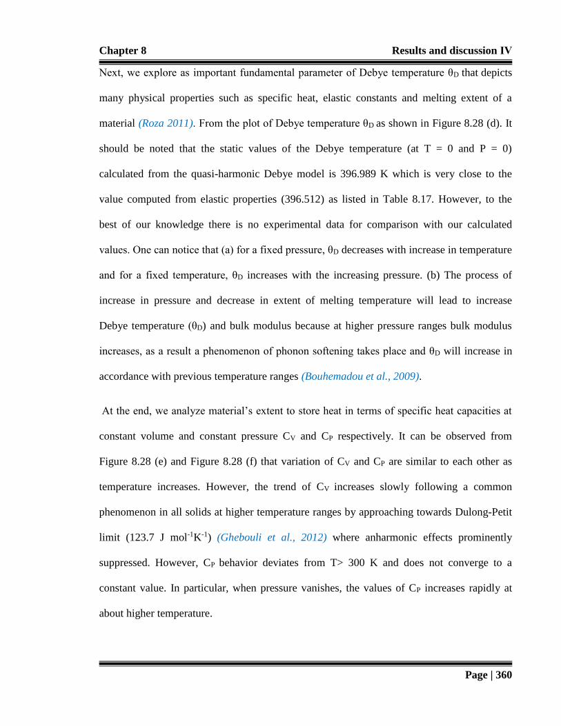
Chapter 8 Results and discussion ΙV
Page | 360
Next, we explore as important fundamental parameter of Debye temperature θD that depicts
many physical properties such as specific heat, elastic constants and melting extent of a
material (Roza 2011). From the plot of Debye temperature θD as shown in Figure 8.28 (d). It
should be noted that the static values of the Debye temperature (at T = 0 and P = 0)
calculated from the quasi-harmonic Debye model is 396.989 K which is very close to the
value computed from elastic properties (396.512) as listed in Table 8.17. However, to the
best of our knowledge there is no experimental data for comparison with our calculated
values. One can notice that (a) for a fixed pressure, θD decreases with increase in temperature
and for a fixed temperature, θD increases with the increasing pressure. (b) The process of
increase in pressure and decrease in extent of melting temperature will lead to increase
Debye temperature (θD) and bulk modulus because at higher pressure ranges bulk modulus
increases, as a result a phenomenon of phonon softening takes place and θD will increase in
accordance with previous temperature ranges (Bouhemadou et al., 2009).
At the end, we analyze material’s extent to store heat in terms of specific heat capacities at
constant volume and constant pressure CV and CP respectively. It can be observed from
Figure 8.28 (e) and Figure 8.28 (f) that variation of CV and CP are similar to each other as
temperature increases. However, the trend of CV increases slowly following a common
phenomenon in all solids at higher temperature ranges by approaching towards Dulong-Petit
limit (123.7 J mol-1K-1) (Ghebouli et al., 2012) where anharmonic effects prominently
suppressed. However, CP behavior deviates from T> 300 K and does not converge to a
constant value. In particular, when pressure vanishes, the values of CP increases rapidly at
about higher temperature.

Chapter 8 Results and discussion ΙV
Page | 361
To best of our information there is lack of investigated information on pressure dependent
physical behavior of SrKF3 in cubic phases so hopefully this work will motivate research
scholars to done theoretical as well as experimental studies in this direction, so they can
compare their results with our work to get better beneficial understanding about pressure
dependent behavior of this material.
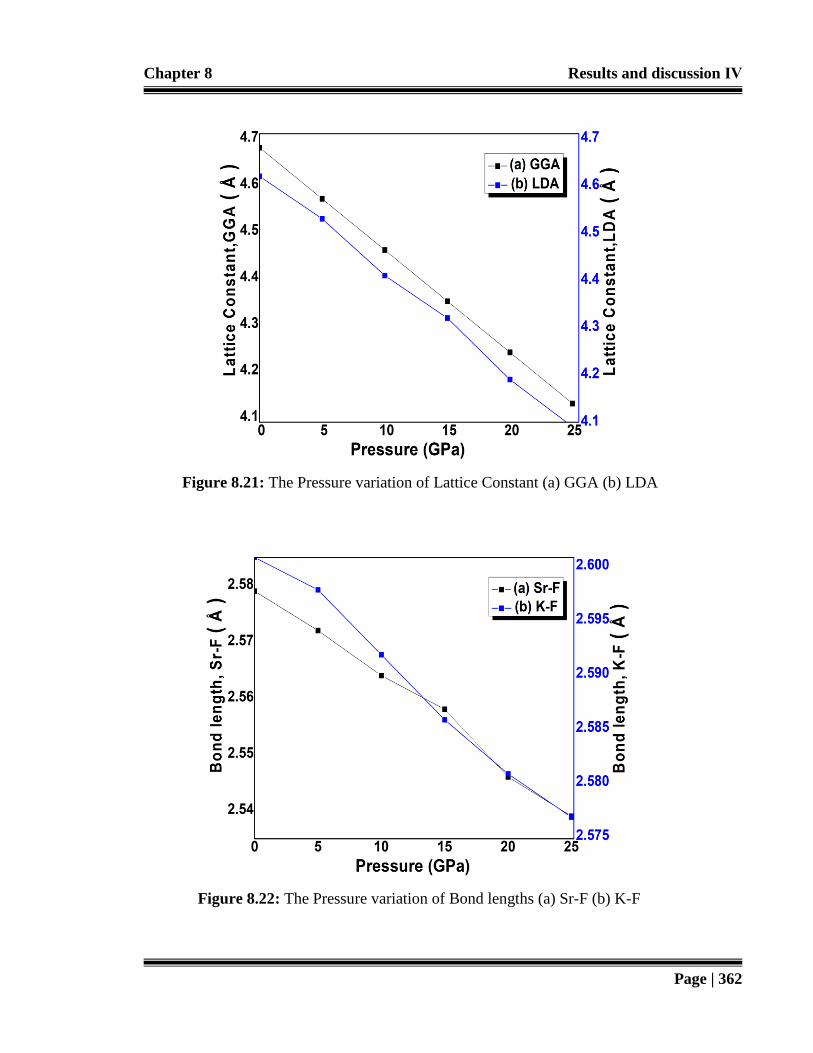
Chapter 8 Results and discussion ΙV
Page | 362
Figure 8.21: The Pressure variation of Lattice Constant (a) GGA (b) LDA
Figure 8.22: The Pressure variation of Bond lengths (a) Sr-F (b) K-F

Chapter 8 Results and discussion ΙV
Page | 363
Figure 8.23: The Pressure dependence of Band Gap (a) GGA (b) mBj
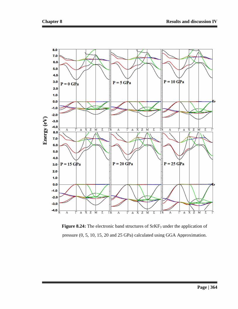
Chapter 8 Results and discussion ΙV
Page | 364
Figure 8.24: The electronic band structures of SrKF3 under the application of
pressure (0, 5, 10, 15, 20 and 25 GPa) calculated using GGA Approximation.
En
ergy
(eV
)

Chapter 8 Results and discussion ΙV
Page | 365
Figure 8.25: The Total and Partial Density of states (TDOS & PDOS) of SrKF3 at
0 and 25 GPa using GGA Approximation.
Energy (eV)
DO
S (
Sta
tes/e
V)

Chapter 8 Results and discussion ΙV
Page | 366
Figure 8.26: Calculated pressure dependence of elastic constants/moduli
(a) C11 (b) C12 (c) C44 (d) Bulk modulus, B for SrKF3 compound.
Figure 8.27: Stability criteria for cubic SrKF3 compound as a
function of pressure.

Chapter 8 Results and discussion ΙV
Page | 367
Figure 8.28 (a): Variation of the Lattice constant as a function of temperature at
different pressures for SrKF3 compound.

Chapter 8 Results and discussion ΙV
Page | 368
Figure 8.28 (b): Variation of the unit cell volume as a function of temperature at
different pressures for SrKF3 compound.

Chapter 8 Results and discussion ΙV
Page | 369
Figure 8.28 (c): Variation of the Bulk modulus as a function of temperature at
different pressures for SrKF3 compound.
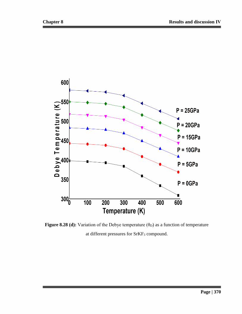
Chapter 8 Results and discussion ΙV
Page | 370
Figure 8.28 (d): Variation of the Debye temperature (θD) as a function of temperature
at different pressures for SrKF3 compound.

Chapter 8 Results and discussion ΙV
Page | 371
Figure 8.28 (e): Variation of the specific heat capacities of Cv as a function of temperature
at different pressures for SrKF3 compound.
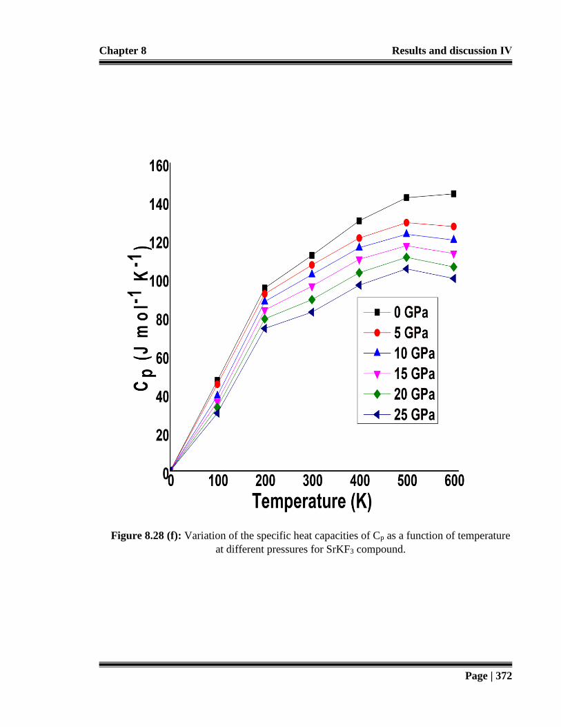
Chapter 8 Results and discussion ΙV
Page | 372
Figure 8.28 (f): Variation of the specific heat capacities of Cp as a function of temperature
at different pressures for SrKF3 compound.

Chapter 8 Results and discussion ΙV
Page | 373
Table 8.13: Comparison of the present calculation with the previous experimental and
theoretical values for the lattice constants (ao), ground state energies (Eo), bulk modulus (Bo)
and its pressure derivative (B′) at ambient pressure of SrKF3 compound.
Compound: SrKF3 Present work Previous work
ao (Å) 4.678 4.680a, 4.656b, 4.629c, 4.49d
Bo (GPa) 38.698 38.692a, 38.121b, 37.125c
B′ (GPa) 2.961 2.991a, b
a) (Mubarak and Mousa 2012), b) (Erum and Iqbal 2016), c) (Erum and Iqbal, March 2017) (Other theoretical
work), d) (Castro 2002) (Experimental Work)
Table 8.14: Comparison of previous and calculated values of Pressure (P in GPa), Energies
(E in Ry), Volume of unit cell (V in (a.u.)3), Energy Gap (eV), and Bond length (dSr-F, dK-F).
a) (Mubarak and Mousa 2012), b) (Erum and Iqbal, March 2017), c) (Erum and Iqbal 2016)
Pressure
(GPa)
Energies
(Ry)
Volume
(a.u.)3
Energy Gap (eV)
Present Present Previous (GGA) (mBJ) (0.00 GPa)
dSr-F
(Ǻ)
dK-F (Ǻ) dX-F (Ǻ) (X= Li,Na,K,Rb)c
0 -8163.848 691.75437 3.307 6.799 3.31a(GGA)
2.579 2.601 dSr-F = 2.57
(0.00 GPa)
5 -8163.820 644.11432 3.537 6.982 3.23b(LDA) 2.572 2.598 dLi-F = 1.85
(0.00 GPa)
10 -8163.804 598.71334 3.633 7.120 3.30b(GGA) 2.564 2.592 dNa-F = 2.23
(0.00 GPa)
15 -8163.795 555.49752 3.727 7.198 6.79b(mBj) 2.558 2.586 dK-F = 2.60
(0.00 GPa)
20 -8163.782 514.41299 3.755 7.235 2.546 2.581 dRb-F = 2.74
(0.00 GPa)
25 -8163.771 475.40584 3.823 7.302 2.539 2.577

Chapter 8 Results and discussion ΙV
Page | 374
Table 8.15: Calculated values of elastic constants (C11, C12, C44) of SrKF3 at pressure from
0-25 GPa.
a) (Erum and Iqbal 2016)
Table 8.16: Calculated values of Bulk modulus (B0), Voigt’s shear modulus (GV), Reuss’s
shear modulus (GR) and Hill’s shear modulus (GH), Young’s modulus (Y), and B/G ratio of
SrKF3 at pressure from 0-25 GPa.
a) (Erum and Iqbal 2016), b) (Mubarak and Mousa 2012), c) (Erum and Iqbal, March 2017)
Pressure (GPa) 0 5 10 15 20 25 Previous
Work
(0.00 GPa)
C11 (GPa) 98.101 123.268 152.542 179.842 207.197 238.746 98.230a
C12 (GPa) 9.021 17.289 26.598 37.128 44.895 54.385 9.019a
C44 (GPa) 20.189 21.221 22.985 23.682 23.998 24.512 20.170a
Pressure
(GPa)
0 5 10 15 20 25 Previous
Work
(0.00 GPa)
Bo(GPa) 38.71 53.71 71.12 85.26 104.07 119.74 38.423a, 37.691b,
37.925c
Gv(GPa) 29.929 33.928 38.980 42.752 46.859 51.579 29.854a,
GR(GPa) 25.840 27.915 30.811 32.319 33.410 34.702 25.794a
GH(GPa) 27.885 30.922 34.895 37.536 40.135 43.140 27.884a
Y(GPa) 67.457 77.830 89.971 98.197 106.689 115.545 67.397a
B/G (GPa) 1.388 1.737 2.038 2.271 2.593 2.776 1.375a

Chapter 8 Results and discussion ΙV
Page | 375
Table 8.17: Calculated values of Poisson’s ratio (ѵ), Cauchy pressure (C’’), Anisotropy
constant (A), Kleinman parameter (ξ), melting temperature (Tm), longitudinal (υl in m/s),
transverse (υt in m/s), average sound velocity (υm in m/s), and Debye temperature (θD in K)
of SrKF3 at pressure from 0-25 GPa.
a) (Erum and Iqbal 2016)
Pressure
(GPa)
0 5 10 15 20 25 Previous
Work
(0.00 GPa)
Ѵ (GPa) 0.210 0.258 0.289 0.308 0.329 0.339 0.210a
C'' -11.168 -3.932 3.613 13.446 20.897 29.873 -11.167a
A (GPa) 0.453 0.400 0.365 0.332 0.296 0.266 0.451a
ξ(GPa) 0.255 0.316 0.360 0.403 0.416 0.431 0.256a
Tm(K) 1522.00 1661.50 1823.42 1954.92 2129.85 2275.58 1522.26a
υl (m/s) 2597.780 2733.618 2902.544 3007.808 3106.828 3217.591 ----
υt (m/s) 4285.592 4789.912 5329.490 5710.698 6156.192 6522.205 ----
υm (m/s) 3288.003 3520.575 3783.154 3951.142 4118.743 4284.748 ----
θD(K) 396.592 442.814 481.950 518.056 549.218 578.968 ----

Chapter 8 Results and discussion ΙV
Page | 376
Table 8.18: Derived elastic constants characterizing mechanical stability (equation 8.36-
8.38) of SrKF3 at pressure from 0-25 GPa.
Pressure (GPa) M1 M2 M3
0 38.71 20.19 44.54
5 54.28 16.22 47.99
10 71.91 12.99 52.97
15 89.70 8.68 56.36
20 105.66 4.00 61.15
25 124.17 -0.49 67.18
Chapter 8 Results and discussion ΙV
Page | 377
8.6 Pressure variation on physical properties of SrRbF3
In this section, Density functional theory (DFT) is employed to calculate the effect of
pressure variation on electronic structure, elastic parameters, mechanical durability, and
thermodynamic aspects of SrRbF3. For the total energy calculations, the Full-Potential
Linearized Augmented Plane Wave (FP-LAPW) method (Schwarz et al., 2010) is employed.
Thermodynamic properties are computed in terms of Quasi-harmonic Debye model (Blanco
et al., 2004), within 0-25 GPa pressure and 0-600 K temperature.
8.6.1 Pressure variation on structural properties
The fluoroperovskite SrRbF3 compound has an ideal cubic structure with space group Pm-3m
(no. 221) at ambient conditions. To determine the structural properties the total energy is
calculated at different volumes (Murnaghan 1944). The details of various lattice parameters,
tolerance factor, bond lengths, bulk modulus, and its pressure derivative at zero pressure are
previously reported in chapter 5 (Erum and Iqbal, March 2017 & Erum and Iqbal 2016).
However, for the continuation of thesis, brief form of previously calculated lattice parameters
is mentioned in Table 8.19, at constant (zero) pressure. The main aim of this section is to
investigate pressure variation consequences on structural properties and mechanic aspects of
SrRbF3 within 0-25 GPa, with step size of 5 GPa as revealed in Table 8.20. Plot of lattice
constant by GGA and LDA schemes are shown in Figure 8.29. Here, compression results
decrease in lattice constants and bond lengths both for Sr-F and Rb-F as displayed in Figure
8.30 respectively, in similar accordance with our/others published work (Erum and Iqbal,
December 2017 , Erum and Iqbal, November 2017, Erum and Iqbal, September 2017, Erum
and Iqbal, March 2017, Erum and Iqbal 2016; Düvel et al., 2011 & Korba et al., 2009).

Chapter 8 Results and discussion ΙV
Page | 378
8.6.2 Pressure variation on elastic properties
The elastic properties have been investigated by using Charpin method. Furthermore, within
the Charpin method the elastic properties of cubic crystals are elucidated by the elastic
constants namely C11, C12, and C44 respectively (Charpin 2001). The computed values of the
C11, C12, and C44 are presented in Table 8.21, which shows reasonable agreement with
previous work (Erum and Iqbal 2016) at fixed (zero) pressure. The focus of this section is to
examine the effect of pressure variation on shear strength, tensile strength, rigidity of the
investigated compound whom calculational details can be found in previous section 8.3.3-
8.3.4 and in the following references (Shafiq et al., 2015; Brik 2011 & Kleinman 1962).
The deformation of material under any small stresses can characterized by elastic constants
(Pettifor 1992). Figure 8.31 presents effect of pressure variation on elastic moduli such as
C11, C12, and C44 respectively. From Figure 8.31 and Table 8.21, it can be observed that with
the rise in compression the value of all elastic constants increases. The C11, which is related
to elasticity in length improve with pressure which means that pressure enhance tensile
strength of SrRbF3 compound. The increase in C11, can be described in terms of enhancement
in bond strength (Sr-F, and Rb-F) because there is decrease in the bonds length and increase
in charge density at elevated pressure ranges. The C44 elastic constant, which is related to
shape deformation, becomes less effected against elevated pressure that indicates less bond
strength enhancement. To check cubic phase stability of SrRbF3, the derived elastic stability
conditions are shown in Table 8.22 within pressure range from 0-25 GPa. It is evident that
compound obey the cubic stability conditions (Wang et al., 1993) and modified stability
criteria (Sadd 2005) for cubic crystals under finite strain till 20 GPa. It can be perceived from
Figure 8.32 that considered elastic constants do not obey stability condition, M2 as mentioned

Chapter 8 Results and discussion ΙV
Page | 379
in section 8.3.3, 8.4.3, and 8.5.3 because at 25 GPa pressure stability criteria of M2 value is
lower than zero (-2.84), which implies that calculated elastic constants cannot satisfy all
mechanical stability conditions, hence the compound is not mechanically stable above 20
GPa. As a result, it can be ensured that SrRbF3 undergo no structural phase transition for
pressure up to 20 GPa.
8.6.3 Pressure variation on mechanical properties
This section is dedicated to calculate effect of hydrostatic pressure on mechanical properties
of SrRbF3 compound according to some proposed mathematical relationships as cited in the
following reference (Shafiq et al., 2015; Brik 2011 & Kleinman 1962) and whom
calculational details can be found in previous section 8.3.3-8.3.4 as well. From the trend of
elastic moduli, as shown in Figure 8.33 and Table 8.23-8.24, such as Young’s modulus (Y),
Bulk modulus (B0), Reuss’s shear modulus (GR), Voigt’s shear modulus (GV), and Hill’s
shear modulus (GH), it can be observed that SrRbF3 has highest value of stiffness and rigidity
at pressure of 25 GPa and lowest value of stiffness and rigidity at 0 GPa pressure. It depicts
material becomes stiffer and less compressible when applied pressure is increased. These
results are in reasonable accordance with the previous work related to perovskite compounds
under the influence of varying pressure by Rai and his fellows (Rai et al., 2014).
Furthermore, SrRbF3 changes its behavior from brittle to ductile character, one as pressure
changes from 0 to 25 GPa. In accordance with our previous work (Jenkins & Khanna 2005)
B/G less than 1.75 confirms, compound is brittle in character, on the other hand, its value
greater than 1.75 classifies compound as ductile. Poisson’s ratio (ѵ) reveals similar trend of
behavior with the change in pressure. The anisotropy elastic factor (A), interprets an increase
in degree of deviation with the increased pressure. The Kleinman parameter can be used to

Chapter 8 Results and discussion ΙV
Page | 380
analyze bond bending (Kleinman 1962), that is basically consistent with above mentioned
results. The trend of melting temperature depicts that an increase in pressure induces less
tendency of melting extent for SrRbF3 compound, which eventually increases its melting
temperature.
8.6.4 Pressure variation on Debye temperature (θD)
The Debye temperature (θD) explores the crystal’s response towards vibration. Above this
temperature crystal behaves classically. In this investigation we use elastic constant method
to perform these calculations as show in Table 8.24. The details of this method and about
their related formulas can be found in section 8.5.5 and in following references (Rached et
al., 2009; Schreiber and Anderson 1973 & Anderson 1963) as well. Figure 8.34 (a) depicts
effect of pressure variation within (0-25 GPa) on average, longitudinal, and transverse wave
velocities as a function of pressure (0- 25 GPa). A prominent quadratic variation in wave
velocities can be observed which monotonically increases with the increase in pressure. In
fact, longitudinal wave velocity increases rapidly as compared to shear wave velocity. The
increasing trend of θD, as shown in Figure 8.34 (b) and Table 8.24, is in similar accordance
with elastic wave velocity. Furthermore, increase in θD is in direct relation with bulk modulus
because of the fact that its high value persuades phonon softening within the applied
pressure.
8.6.5 Pressure and temperature variations on thermodynamic properties
The thermodynamic properties of SrRbF3 are determined using Quasi-harmonic Debye
model as implemented in the Gibbs program (Blanco et al., 2004). Through this model, we
can get all thermodynamic quantities from the calculated energy-volume data. The calculated
details can be seen in the previously published work (Francisco et al., 2001; Francisco et al.,

Chapter 8 Results and discussion ΙV
Page | 381
1998 & Greiner et al., 1995) and in section 8.3.5 as well. The pressure effects are determined
in the range of 0-25 GPa, in which cubic stability of SrRbF3 fluoroperovskite remains valid
and thermal properties are studied in temperature range from 0 to 600 K.
Figure 8.35 (a) and Figure 8.35 (b) presents the relation between lattice parameters (lattice
constant and unit cell volume) and Figure 8.35 (c) presents isothermal bulk modulus with
temperature T up to 600 K at P = 0 GPa, 5 GPa, 10 GPa, 15 GPa, 20 GPa, and 25 GPa
respectively. It can be noticed that both temperature and pressure have inverse relation with
lattice parameters and bulk modulus because at a given pressure lattice parameters such as
lattice constants and volume expansion increase with the increasing temperature and bulk
modulus decreases with increasing temperature at a given pressure and vice-versa. In fact, at
higher pressure thermal effects becomes weaker as well as stronger for lattice parameters and
bulk modulus respectively (Ghebouli et al., 2012), which reveals that effect of pressure and
temperature are inversely proportional to each other. So, increase in temperature causes a
significant reduction in the hardness of SrRbF3.
The Debye cut-off frequency or Debye temperature (θD) is important due to extraction of
some useful physical quantities for example specific heat capacities and melting point
(Bouhemadou et al., 2009). Figure 8.35 (d) reveals that value of θD remains smooth till 100 K
and for temperature greater than 200 K it decreases monotonically. While for a constant
temperature, θD rises linearly with pressure.
However, at zero pressure and ambient temperature, our calculated θD from elastic constant
method is 362.019 K, as shown in Table 8.24, which are closer from calculated values to the
quasi-harmonic model as shown in Figure 8.35 (d). The specific constant volume heat

Chapter 8 Results and discussion ΙV
Page | 382
capacity CV and constant pressure heat capacity CP are shown in Figure 8.35 (e) and Figure
8.35 (f). It can be observed from figures that variation of CV and CP with the increase in
temperature are similar to each other. Further, the trend of CV rises gradually and inclines to
move in the direction of Dulong-Petit limit which is 123.7 J mol-1K-1, a common
phenomenon in all solids at high temperature ranges (Rached et al., 2009). Moreover, the
anharmonic effects are also suppressed at high temperature. However, CP decreases as
increase in pressure from (0- 25 GPa) and deviation is observed with a constant value. So, at
ambient pressure, the values of CP increase quickly at elevated temperature ranges.
To best of our information there is lack of investigated information on pressure dependent
physical behavior of SrRbF3 in cubic phases so hopefully this work will motivate research
scholars to done theoretical as well as experimental studies in this direction, so they can
compare their results with our work to get better beneficial understanding about pressure
dependent behavior of this material.

Chapter 8 Results and discussion ΙV
Page | 383
Figure 8.29: The Pressure variation of Lattice Constant (a) GGA (b) LDA
Figure 8.30: The Pressure variation of Bond lengths (a) Sr-F (b) Rb-F

Chapter 8 Results and discussion ΙV
Page | 384
Figure 8.32: Stability criteria for cubic SrRbF3 compound
as a function of pressure.
Figure 8.31: Calculated pressure dependence of elastic constants
(a) C11 (b) C12 (c) C44 for SrRbF3 compound.

Chapter 8 Results and discussion ΙV
Page | 385
Figure 8.33: Calculated pressure dependence of elastic parameters (a) Bulk
modulus (B) (b) Shear modulus (G) (c) Young’s modulus (Y) (d) B/G Ratio
for SrRbF3 compound.
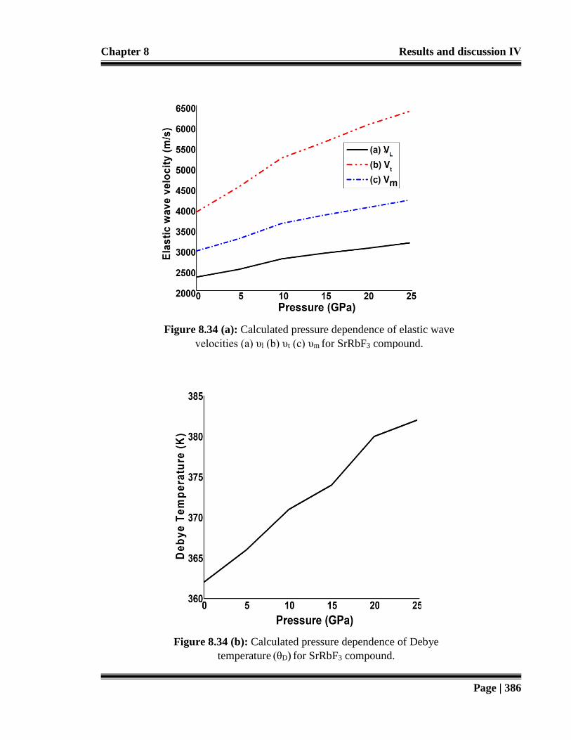
Chapter 8 Results and discussion ΙV
Page | 386
Figure 8.34 (a): Calculated pressure dependence of elastic wave
velocities (a) υl (b) υt (c) υm for SrRbF3 compound.
Figure 8.34 (b): Calculated pressure dependence of Debye
temperature (θD) for SrRbF3 compound.
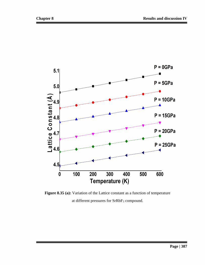
Chapter 8 Results and discussion ΙV
Page | 387
Figure 8.35 (a): Variation of the Lattice constant as a function of temperature
at different pressures for SrRbF3 compound.

Chapter 8 Results and discussion ΙV
Page | 388
Figure 8.35 (b): Variation of the unit cell volume as a function of temperature
at different pressures for SrRbF3 compound.

Chapter 8 Results and discussion ΙV
Page | 389
Figure 8.35 (c): Variation of the Bulk modulus as a function of temperature
at different pressures for SrRbF3 compound.

Chapter 8 Results and discussion ΙV
Page | 390
Figure 8.35 (d): Variation of the Debye temperature (θD) as a function of temperature
at different pressures for SrRbF3 compound.

Chapter 8 Results and discussion ΙV
Page | 391
Figure 8.35 (e): Variation of the specific heat capacities of Cv as a function of temperature
at different pressures for SrRbF3 compound.

Chapter 8 Results and discussion ΙV
Page | 392
Figure 8.35 (f): Variation of the specific heat capacities of Cp as a function of temperature
at different pressures for SrRbF3 compound.

Chapter 8 Results and discussion ΙV
Page | 393
Table 8.19: Comparison of the present calculation with the previous experimental and
theoretical values for the lattice constants (ao), ground state energies (Eo), bulk modulus (Bo)
and its pressure derivative (B′) at ambient pressure for SrRbF3 compound.
a) (Mubarak and Mousa 2012), b) (Erum and Iqbal 2016), c) (Erum and Iqbal, March 2017) (Other theoretical
work), d) (Castro 2002) (Experimental Work)
Table 8.20: Comparison of previous and calculated values of Pressure (P in GPa), Energies
(E in Ry), Volume of unit cell (V in (a.u.)3) and Bond length (dSr-F, dRb-F) of SrRbF3
compound.
a) (Erum and Iqbal, September 2017), b) (Erum and Iqbal 2016)
Compound: SrRbF3 Present work Previous work
ao (Å) 4.947 4.952a, 4.938b, 4.940c, 4.479d
Bo (GPa) 33.098 32.902a, 33.121b, 33.105c
B′ (GPa) 4.009 4.010a, b
Pressure
(GPa)
Energies
(Ry)
Volume
(a.u.)3
dSr-F (Ǻ) dSr-F (Ǻ)
(SrKF3) a
dRb-F
(Ǻ)
dK-F (Ǻ)
(SrKF3) a dX-F (Ǻ)
(0.00 GPa) (X= Li,Na,K,Rb)b
0 -12922.44 818.52124 2.601 2.579 2.742 2.601 dSr-F = 2.57
5 -12922.41 769.90931 2.598 2.572 2.738 2.598 dLi-F = 1.85
10 -12922.37 727.83882 2.586 2.564 2.732 2.592 dNa-F = 2.23
15 -12922.34 678.53650 2.581 2.558 2.729 2.586 dK-F = 2.60
20 -12922.29 644.11432 2.575 2.546 2.724 2.581 dRb-F = 2.74
25 -12922.25 606.80395 2.569 2.539 2.718 2.577

Chapter 8 Results and discussion ΙV
Page | 394
Table 8.21: Calculated values of elastic constants (C11, C12, C44) of SrRbF3 at pressure from
0-25 GPa.
a) (Erum and Iqbal 2016), b) (Erum and Iqbal, September 2017), c) (Erum and Iqbal, December 2017)
Table 8.22: Calculated values of derived elastic constants characterizing mechanical stability
of SrRbF3 at pressure from 0-25 GPa.
a) (Erum and Iqbal, September 2017), b) (Erum and Iqbal, December 2017)
Pressure
(GPa)
0 5 10 15 20 25 Previous
Work (0.00 GPa)
(SrRbF3) a
Previous
Work (25.00 GPa)
(SrKF3) b
Previous
Work (25.00 GPa)
(SrNaF3) c
C11
(GPa)
85.251 112.525 150.256 175.021 205.895 225.284 85.230 238.746 429.043
C12
(GPa)
6.881 12.102 16.258 21.121 26.598 32.427 6.819 54.385 61.098
C44
(GPa)
14.091 15.289 17.021 18.992 20.021 22.158 14.170 24.512 25.98
Pressure (GPa) 0 5 10 15 20 25 Previous
Work (25.00 GPa)
(SrKF3) a
Previous
Work (25.00 GPa)
(SrNaF3) b
M1 33.05 47.24 64.26 77.42 93.03 105.05 124.17 64.94
M2 14.09 10.29 7.02 3.99 0.02 -2.84 -0.49 -2.57
M3 39.26 45.21 57.00 61.95 69.65 71.43 67.18 41.68

Chapter 8 Results and discussion ΙV
Page | 395
Table 8.23: Calculated values of Bulk modulus (B0), Voigt’s shear modulus (GV), Reuss’s
shear modulus (GR) Hill’s shear modulus (GH), Young’s modulus (Y), and B/G ratio of
rRbF3 at pressure from 0-25 GPa.
a)(Erum and Iqbal 2016), b)(Mubarak 2014), c)(Erum and Iqbal, March 2017), d)(Erum and Iqbal, September
2017)
Table 8.24: Calculated values of Poisson’s ratio (ѵ), Cauchy pressure (C’’), Anisotropy
constant (A), Kleinman parameter (ξ), melting temperature (Tm), longitudinal (υl in m/s),
transverse (υt in m/s), average sound velocity (υm in m/s), and Debye temperature (θD in K)
of SrRbF3 at pressure from 0-25 GPa.
a) (Erum and Iqbal 2016), b)(Mubarak 2014), c)(Erum and Iqbal, March 2017), d)(Erum and Iqbal, September
2017)
Pressure
(GPa)
0 5 10 15 20 25 Previous
Work
(0.00 GPa)
Previous
Work (25.00 GPa)
(SrKF3) d
Bo(GPa) 32.129 48.125 68.254 82.84 101.245 114.256 32.123a,
33.691b,
32.125c
119.74
Gv(GPa) 24.158 29.258 37.012 42.175 47.872 51.866 24.154a, 51.579
GR(GPa) 18.750 21.182 24.260 27.181 29.044 32.024 18.794a 34.702
GH(GPa) 21.554 25.220 30.636 34.678 38.458 41.945 21.884a 43.140
Y(GPa) 52.845 64.409 79.946 91.295 102.408 112.116 52.897a 115.545
B/G (GPa) 1.491 1.908 2.228 2.389 2.633 2.724 1.495a 2.776
Pressure
(GPa)
0 5 10 15 20 25 Previous
Work (0.00 GPa)
(SrRbF3) a
Previous
Work (25.00 GPa)
(SrKF3) d
Ѵ (GPa) 0.226 0.277 0.305 0.316 0.331 0.336 0.225 0.339
C'' -7.210 -3.187 -0.763 2.129 6.577 10.269 -7.167 29.873
A (GPa) 0.359 0.304 0.254 0.247 0.223 0.230 0.358 0.266
ξ(GPa) 0.240 0.274 0.275 0.291 0.302 0.321 0.242 0.431
Tm(K) 1460.80 1609.56 1796.76 1932.41 2103.58 2224.58 1461.11 2275.58
υl (m/s) 2326.274 2513.802 2767.831 2907.567 3024.201 3156.458 ---- 3217.591
υt (m/s) 3909.211 4525.923 5223.247 5609.545 6022.603 6357.950 ---- 6522.205
υm (m/s) 2961.153 3260.925 3631.182 3833.188 4013.397 4198.241 ---- 4284.748
θD(K) 362 366 371 374 380 382 ---- 578.968

Chapter 8 Results and discussion ΙV
Page | 396
8.7 Pressure variation on physical properties of CaLiF3
In this section, the effect of pressure variation on electronic structure, elastic constants,
mechanical stability, and thermodynamic characteristics of cubic CaLiF3 fluoroperovskite
have been investigated by employing first-principles method. For the total energy
calculations, the Full-Potential Linearized Augmented Plane Wave (FP-LAPW) method
(Schwarz et al., 2010) is employed. Thermodynamic properties are computed in terms of
Quasi-harmonic Debye model (Blanco et al., 2004), within 0-50 GPa pressure and 0-600 K
temperature.
8.7.1 Pressure variation on structural properties
The structural properties are determined via different volumes over a range ± 10% which are
selected to calculate minimum ground state energy (EO) at zero pressure. Here Birch
Murnaghan’s equation of state (EOS) (Murnaghan 1944) is used to fit the minimum energy
(EO) versus minimum volume (VO). The calculated ground state lattice parameters (at zero
pressure) such as lattice constant of the present work is 3.687 Å, as shown in Table 8.25, is in
good agreement with previously reported theoretical/ experimental work (Mousa et al., 2013;
Mishra et al., 2011; Ouenzerfi 2004 & Castro 2002).
In order to examine the crystal structure of CaLiF3 on different hydrostatic pressure (0 to 50
GPa), we attempt to study the effect of different pressure, with a step size of 10 GPa, on
lattice parameters. Figure 8.36 depicts calculated change in the value of lattice constant by
LDA and GGA approximations. It can be interpreted that lattice constant is going to decrease
both by LDA and GGA approximations. The variation of bond lengths Ca-F and Li-F with
pressure is also presented in Figure 8.37. However, with comparison of data at constant
pressure of the same series as shown in Table 8.26 (Erum and Iqbal 2016), it can be analyzed

Chapter 8 Results and discussion ΙV
Page | 397
that Li-F and Ca-F bond lengths compress to a reasonable extent within the limit that
constituent polyhedral of CaLiF3 do not become distorted with the change in the pressure.
The reduction in values of bond lengths and lattice constant can be associated via difference
of bandgap and hybridization strength which is previously discussed in section 8.3.
8.7.2 Pressure variation on elastic properties
The elastic properties have been investigated by using Charpin method. Furthermore, within
the Charpin method the elastic properties of cubic crystals are elucidated by the elastic
constants namely C11, C12, and C44 respectively (Charpin 2001). The computed values of the
C11, C12, and C44 are presented in Table 8.27, which shows reasonable agreement with
previous work (Erum and Iqbal 2016) at fixed (zero) pressure. The focus of this section is to
examine the effect of pressure variation on shear strength, tensile strength, rigidity of the
investigated compound whom calculational details can be found in previous section 8.3.3-
8.3.4 and in the following references (Shafiq et al., 2015; Brik 2011 & Kleinman 1962).
The deformation of material under any small stresses can characterized by elastic constants
(Pettifor 1992). Figure 8.38 presents effect of pressure variation on elastic moduli such as
C11, C12, and C44 respectively. From Figure 8.38 and Table 8.27 it can be observed that with
the rise in compression all elastic constants increase. Elasticity in length C11, is observed with
increase in pressure. The growth in C11 can be described in terms with enhancement in bond
strength (Ca-F, and Li-F) because there is decrease in the bond lengths and increase of charge
density at elevated pressure ranges. The shape deformation elastic moduli become less
effected against elevated pressure that indicates less bond strength enhancement. It is evident
that compound obey the cubic stability conditions (Wang et al., 1993) and modified stability
criteria (Sadd 2005) for cubic crystals under finite strain till 40 GPa. It can be perceived from

Chapter 8 Results and discussion ΙV
Page | 398
Figure 8.39 that considered elastic constants do not obey stability condition, M2 as mentioned
in section 8.3.3, 8.4.3, and 8.5.3 because at 50 GPa pressure stability criteria of M2 value is
lower than zero (-4.55), which implies that calculated elastic constants cannot satisfy all
mechanical stability conditions, hence the compound is not mechanically stable above 40
GPa. As a result, it can be ensured that CaLiF3 undergo no structural phase transition for
pressure up to 40 GPa.
8.7.3 Pressure variation on mechanical properties
The elastic parameters (calculated in previous section) relates thermal and mechanical
behavior of compound (Shafiq et al., 2015). This section is dedicated to calculate effect of
hydrostatic pressure on mechanical properties of CaLiF3 compound according to some
proposed mathematical relationships as cited in the following reference (Brik 2011 &
Kleinman 1962) and whom calculational details can be found in previous section 8.3.3-8.3.4
as well. From the trend of Young’s modulus (Y), Bulk modulus (B0), Reuss’s shear modulus
(GR), Voigt’s shear modulus (GV), and Hill’s shear modulus (GH), it can be observed that
CaLiF3 has highest value of stiffness and rigidity at pressure of 50 GPa and lowest value of
stiffness and rigidity at 0 GPa pressure which means that material becomes stiffer and less
compressible when applied pressure is increased, as shown in Figure 8.40. These results are
in reasonable accordance with the previous work related to perovskite compounds under the
influence of varying pressure by Rai and his fellows (Rai et al., 2014).
Furthermore, CaLiF3 changes its behavior from brittle character into ductile one as pressure
changes from 0 to 50 GPa in accordance with work done by Jenkins and Khanna (Jenkins &
Khanna 2005) that, the B/G less than 1.75 conforms material’s brittle character, on the other
hand, its value greater than 1.75 makes compound as ductile. Poisson’s ratio (ѵ) reveals the

Chapter 8 Results and discussion ΙV
Page | 399
alike trend with pressure change. The anisotropy elastic factor (A), interprets an increase in
the degree of deviation with increased pressure. The Kleinman parameter can be used to
analyze bond bending (Kleinman 1962), that is basically consistent with above mentioned
results. Next, we found that an application of hydrostatic compression induces less tendency
of melting extent for calcium based fluoroperovskite.
8.7.4 Pressure variation on Debye temperature (θD)
The Debye temperature (θD) explores the crystal’s response towards vibration. In this
investigation we use elastic constant method to perform these calculations. Above θD crystal
behaves classically. Here, method based on elastic constant is employed to calculate θD. The
details of this method and about their related formulas can be found in section 8.5.5 and in
following references (Rached et al., 2009; Schreiber and Anderson 1973 & Anderson 1963)
as well. Figure 8.41 (a) depicts effect of pressure variation within (0-50 GPa) on average,
longitudinal, and transverse wave velocities as a function of pressure (0- 50 GPa). A
prominent quadratic variation in wave velocities can be observed which monotonically
increases with the every 10 GPa increase in pressure. In fact, longitudinal wave velocity
increases rapidly as compared to shear wave velocity. The increasing trend of θD is also in
similar accordance with elastic wave velocity as shown in Figure 8.41 (b). Furthermore,
increase in θD is in direct relation with bulk modulus because of the fact that its high value
persuades phonon softening within the applied pressure.
8.7.5 Pressure and temperature variations on thermodynamic properties
These parameters of a material provide a way that gives contributing factors in development
of thermodynamic chemistry and solid-state physics. These aspects of CaLiF3 are determined

Chapter 8 Results and discussion ΙV
Page | 400
using Quasi-harmonic Debye model as implemented in the Gibbs program (Blanco et al.,
2004 & Francisco et al., 1998). In this model, from the calculated energy-volume data all
thermodynamic quantities can be evaluated. The details of this method and about their related
formulas can be found in section 8.5.5 and in following references (Rached et al., 2009;
Schreiber and Anderson 1973 & Anderson 1963) as well. In this study thermal properties are
analyzed within 0 to 600 K range with pressure variation within 0-50 GPa range. The specific
constant volume heat capacity CV and constant pressure heat capacity CP are shown in Figure
8.42 (a) and Figure 8.42 (b). It can be observed from figures that variation of CV and CP with
the increase in temperature are similar to each other. Further, the trend of CV rises gradually
and inclines to move in the direction of Dulong-Petit limit which is 123.7 J mol-1K-1, as is
common phenomenon in all solids at high temperature (Bouhemadou et al., 2009). Moreover,
the anharmonic effects are suppressed at high temperature. However, CP decreases as
increase in pressure from (0- 50 GPa) and deviation is observed from a constant value. So, at
ambient pressure, the values of CP increase quickly at elevated temperature. The discrepancy
of the volume (expansion) coefficient α(T) for CaLiF3, is given by the Figure 8.42 (c). It can
be clearly seen that α exhibits enhanced growth for low temperature values and then
progressively tends to rise linearly at elevated temperature ranges. It should be noted that the
progress of α with the temperature becomes smaller as the pressure rises. However, for a
given temperature, α decreases sharply with increasing pressure. The Debye cut-off
frequency or Debye temperature (θD) is important due to extraction of some useful physical
quantities for example specific heat capacities and melting point (Anderson 1963). Figure
8.42 (d) reveals that value of θD remains smooth till 100 K and for temperature greater than
200 K it decreases monotonically. While for a constant temperature, θD rises linearly with

Chapter 8 Results and discussion ΙV
Page | 401
pressure. However, at zero pressure and ambient temperature, our calculated θD from elastic
constant method is 649.019 K which are closer to calculated values from the quasi-harmonic
model.
To best of our information there is lack of investigated information on pressure dependent
physical behavior of CaLiF3 in cubic phases so hopefully this work will motivate research
scholars to done theoretical as well as experimental studies in this direction, so they can
compare their results with our work to get better beneficial understanding about pressure
dependent behavior of this material.

Chapter 8 Results and discussion ΙV
Page | 402
Figure 8.36: The Pressure variation of Lattice Constant (a) LDA (b) GGA
Figure 8.37: The Pressure variation of Bond lengths (a) Ca-F (b) Li-F

Chapter 8 Results and discussion ΙV
Page | 403
Figure 8.39: Stability criteria for cubic CaLiF3 compound as a function of pressure.
Figure 8.38: Calculated pressure dependence of elastic constants (a) C11 (b) C12 (c) C44
for CaLiF3 compound.

Chapter 8 Results and discussion ΙV
Page | 404
Figure 8.40: Calculated pressure dependence of isotropic elastic parameters (a) Bulk
modulus (B) (b) Shear modulus (G) (c) Young’s modulus (Y) (d) B/G ratio for CaLiF3
compound.

Chapter 8 Results and discussion ΙV
Page | 405
Figure 8.41 (b): Calculated pressure dependence of Debye temperature (θD)
for CaLiF3 compound.
Figure 8.41 (a): Calculated pressure dependence of elastic wave velocities
(a) υl (b) υt (c) υm for CaLiF3 compound.
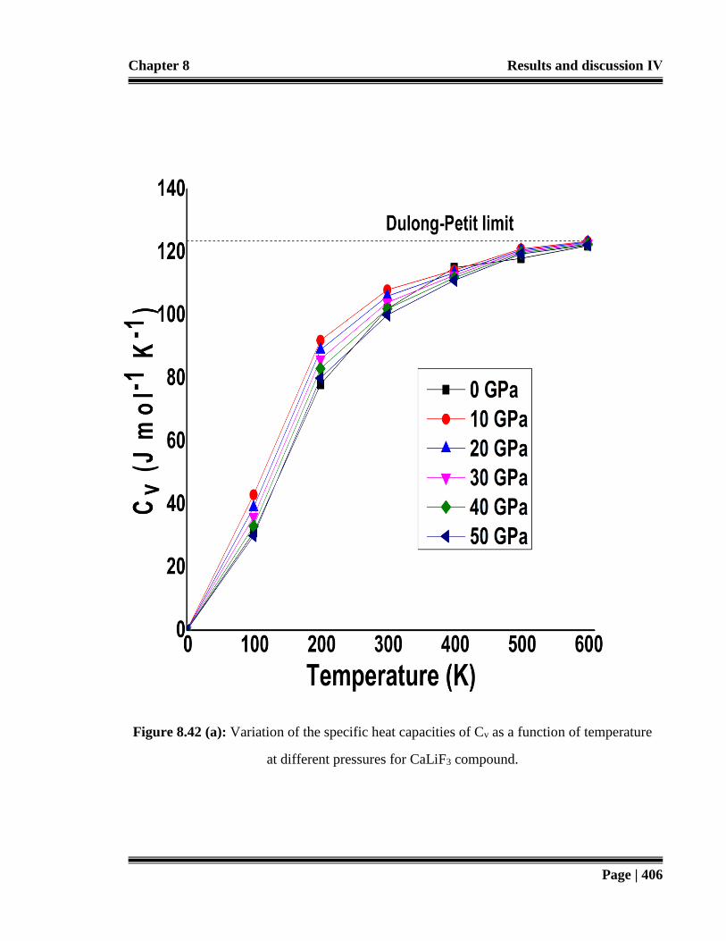
Chapter 8 Results and discussion ΙV
Page | 406
Figure 8.42 (a): Variation of the specific heat capacities of Cv as a function of temperature
at different pressures for CaLiF3 compound.

Chapter 8 Results and discussion ΙV
Page | 407
Figure 8.42 (b): Variation of the specific heat capacities of Cp as a function of temperature
at different pressures for CaLiF3 compound.

Chapter 8 Results and discussion ΙV
Page | 408
Figure 8.42 (c): Temperature dependence of the volume expansion coefficient α(T)
at different pressures for CaLiF3 compound.

Chapter 8 Results and discussion ΙV
Page | 409
Figure 8.42 (d): Variation of the Debye temperature (θD) as a function of temperature
at different pressures for CaLiF3 compound.

Chapter 8 Results and discussion ΙV
Page | 410
Table 8.25: Comparison of the present calculation with the previous experimental and
theoretical values for the lattice constants (ao), ground state energies (Eo), bulk modulus (Bo)
and its pressure derivative (B′) at ambient pressure of CaLiF3 compound.
Compound: CaLiF3 Present
work (LDA)
Present
work (GGA)
Previous work
ao (Å) 3.687 3.772 3.672a, 3.606b, 3.760c
Bo (GPa) 98.87 81.28 98.78b
B′ (GPa) 4.51 4.25 4.43c
a)( Ouenzerfi 2004), b)( Castro 2002) (Experimental Work) c)( Mousa et al., 2013) (Other theoretical work)
Table 8.26: Comparison of previous and calculated values of Pressure (P in GPa), Energies
(E in Ry), Volume of unit cell (V in (a.u.)3) and Bond length (dCa-F, dLi-F) of CaLiF3
compound.
a) (Erum and Iqbal 2016)
Pressure (GPa) Energies (Ry) Volume (a.u.)3 dCa-F (Ǻ) dLi-F (Ǻ) dX-F (Ǻ)
(X=Li,Na,K,Rb)a
0 -6774.891 362.18412 2.531 1.851 dSr-F = 2.57
(0.00 GPa)
10 -6774.863 359.02472 2.527 1.845 dLi-F = 1.85
(0.00 GPa)
20 -6774.855 357.02379 2.521 1.841 dNa-F = 2.23
(0.00 GPa)
30 -6774.839 354.17824 2.518 1.838 dK-F = 2.60
(0.00 GPa)
40 -6774.812 350.50168 2.511 1.832 dRb-F = 2.74
(0.00 GPa)
50 -6774.798 347.41069 2.509 1.828

Chapter 8 Results and discussion ΙV
Page | 411
Table 8.27: Calculated values of elastic constants (C11, C12, C44) of CaLiF3 at pressure from
0-50 GPa.
a) (Erum and Iqbal, November 2017)
Table 8.28: Calculated values of derived elastic constants characterizing mechanical stability
of CaLiF3 at pressure from 0-50 GPa.
a) (Mishra et al., 2011)
Pressure (GPa) 0 10 20 30 40 50 Previous
Work (0.00 GPa)
(SrLiF3) a
C11 (GPa) 156.11 157.254 158.251 160.001 161.017 162.548 157.741
C12 (GPa) 34.351 34.38 34.998 35.105 35.35 36.12 37.353
C44 (GPa) 43.31 43.851 44.014 44.12 45.125 45.452 49.447
Pressure (GPa) 0 10 20 30 40 50 Previous
Work (0.00 GPa)
(BaLiF3) a
M1 74.94 78.67 82.75 86.74 90.57 94.93 73.90
M2 43.31 33.85 24.01 14.12 5.13 -4.55 44.13
M3 60.88 51.44 41.63 32.45 22.83 13.21

Chapter 8 Results and discussion ΙV
Page | 412
Table 8.29: Calculated values of Bulk modulus (B0), Voigt’s shear modulus (GV), Reuss’s
shear modulus (GR), Hill’s shear modulus (GH), Young’s modulus (Y), and B/G ratio, of
CaLiF3 at pressure from 0-50 GPa.
a) (Mousa et al., 2013), b) (Erum and Iqbal, 2016), c) (Mishra et al., 2011)
Table 8.30: Calculated values of Poisson’s ratio (ѵ), Anisotropy constant (A), Kleinman
parameter (ξ), melting temperature (Tm) longitudinal (υl in m/s), transverse (υt in m/s),
average sound velocity (υm in m/s), and Debye temperature (θD in K) of CaLiF3 at pressure
from 0-50 GPa.
a) (Erum and Iqbal, 2016), b) (Mishra et al., 2011)
Pressure (GPa) 0 10 20 30 40 50 Previous
Work
(0.00 GPa)
Bo(GPa) 76.252 77.512 79.285 82.159 86.214 89.128 77.510a
Gv(GPa) 50.338 50.885 51.059 51.451 52.208 52.557 52.515 (SrLiF3) b
GR(GPa) 48.962 49.521 49.695 49.988 50.858 51.207 52.281(SrLiF3) b
GH(GPa) 49.650 50.203 50.377 50.720 51.533 51.882 52.401 (SrLiF3) b,
52.202c
Y(GPa) 122.387 123.867 124.716 126.192 128.915 130.353 127.362 (SrLiF3) b
B/G (GPa) 1.536 1.544 1.574 1.620 1.673 1.718 1.49 (SrLiF3) b
Pressure
(GPa)
0 10 20 30 40 50 Previous
Work (0.00 GPa)
(SrLiF3) a,
b
Ѵ (GPa) 0.232 0.234 0.238 0.244 0.251 0.256 0.215a
A (GPa) 0.711 0.714 0.714 0.707 0.718 0.719 0.81a
0.83b
ξ(GPa) 0.421 0.419 0.422 0.422 0.423 0.424 0.456a
Tm(K) 1871.14 1882.86 1899.35 1926.08 1963.79 1990.89 1854.65a
υl (m/s) 3935.274 4011.802 4142.831 4344.567 4544.201 4656.458 ----
υt (m/s) 6639.011 6798.923 6923.247 7029.545 7122.603 7357.950 ----
υm (m/s) 5054.102 5211.925 5351.182 5533.188 5813.397 5918.241 ----
θD(K) 649 652 657 661 664 667 ----

Chapter 8 Results and discussion ΙV
Page | 413
8.8 Conclusion
In this chapter, effect of hydrostatic pressure on physical properties of five fluoroperovskites
(SrLiF3, SrNaF3, SrKF3, SrRbF3 and CaLiF3) have been carried out successfully.
In Section 8.3, detailed physical properties of SrLiF3 are studied under ambient and high-
pressure ranges. The calculated equilibrium lattice parameters at 0 GPa are in good
agreement with earlier reports. The calculation of elastic properties under various pressure
ranges confirms that the compound is mechanically stable in cubic structure up to 40 GPa.
All elastic and mechanical parameters are linearly dependent on applied pressure. Moreover,
an increase in pressure improves tensile strength and stiffness, on the other hand, reduces
brittleness and compressibility of cubic fluoroperovskite SrLiF3. It is observed that an
increase in pressure considerably improves the wide and direct (Γ-Γ) electronic bandgap
because upon compression bands broadened the energy of Sr-4d and Sr-5d states thereby
resulting an increase in the ratio of splitting between Sr-5d, Sr-4d, Sr-3d, F-2s and F-2p states
which ultimately increase in the bandgap and this increase in bandgap continues upto 50
GPa. All optical responses shift towards higher energy ranges which reveals that SrLiF3 is
more suitable for optoelectronic devices at higher pressure ranges. Finally, thermodynamic
effects on macroscopic properties are predicted to verify application of this compound in
thermodynamic devices in the range 0-50 GPa and 0-600 K. Since SrLiF3 fluoroperovskite
do not undergo any structural phase transition at high pressure so it can be used as an
alternative pressure marker for other materials.
In Section 8.4, we have reported for the first time, detailed theoretical results on effect of
pressure dependence on structural, electronic elastic, mechanical, optical and thermodynamic
Chapter 8 Results and discussion ΙV
Page | 414
properties of cubic SrNaF3 compound based on Density functional theory (DFT). The
calculated lattice parameters at fixed (zero) pressure and temperature are in good agreement
with previous experimental work. The pressure dependence of elastic constants and
significant mechanical parameters confirm compound’s mechanically stability in cubic
structure till 20 GPa. Moreover, an increase in pressure improves tensile strength and
stiffness, on the other hand, reduces brittleness and compressibility of SrNaF3 compound. It
is observed that an increase in pressure considerably improves the wide and direct (Γ-Γ)
electronic bandgap because upon compression bands broadened the energy of Sr-4d and Sr-
5d states thereby resulting in an increase in the ratio of splitting between Sr-5d, Sr-4d, Sr-3d,
F-2s and F-2p states which ultimately increase in the bandgap. All the calculated optical
properties such as the complex dielectric function ε(ω), optical conductivity σ(ω), energy
loss function L(ω), absorption coefficient α(w), refractive index n(ω), reflectivity R(ω), and
effective number of electrons neff, via sum rules shift towards the higher energies under the
application of pressure. Finally, thermodynamic effects on macroscopic properties are
predicted to verify application of this compound in thermodynamic devices using Quasi-
harmonic Debye model in the range 0-25 GPa and 0-600 K. Since increase in pressure
improves elastic and mechanical behavior of SrNaF3 compound, so it can effectively be used
in lens materials. Consequently, we believe that our theoretical results have benchmarked
various quantum mechanical effects at different pressures, which must be taken into account
to understand and utilize in fabricating practical devices.
In Section 8.5, effect of pressure variation on detailed physical properties have investigated
for the first time by ab-inito Density Functional Theory (DFT) method for cubic phase of
SrKF3 fluoroperovskite compound. The calculated equilibrium lattice parameters are in good
Chapter 8 Results and discussion ΙV
Page | 415
agreement with previous theoretical and experimental reports at 0 GPa. It is observed that an
increase in pressure considerably improves the wide and direct (Γ-Γ) electronic nature of
bandgap because at elevated pressure ranges bands broadened the energy of Sr-3d and Sr-4d
states thereby resulting in an increase in the ratio of splitting between Sr-4d, Sr-3d, K-2p, F-
2s and F-2p states which ultimately results an increase in the bandgap of the material. The
pressure dependence of elastic constants and significant mechanical parameters confirm
compound’s mechanically stability in cubic structure till 20 GPa. Moreover, an increase in
pressure improves tensile strength and stiffness, on the other hand, reduces brittleness and
compressibility of the SrKF3 compound. The effect of thermodynamic parameters on
macroscopic properties are predicted to utilize this material in temperature dependent
applications implementing Quasi-harmonic Debye model within the range 0-25 GPa and 0-
600 K with the step size of 5 GPa and 100 K respectively. Consequently, we believe that our
work will motivate research scholars to done theoretical as well as experimental studies in
this direction, which must be taken into account to understand and utilize this material in
fabricating practical devices.
In Section 8.6, physical properties of SrRbF3 under varying pressure are investigated by
using ab-initio study. The calculation of elastic properties under pressure confirms that the
compound is mechanically stable in cubic structure and compound undergo no structural
phase transition, till 20 GPa. All elastic and mechanical parameters are linearly dependent on
applied pressure. Moreover, an increase in pressure reduces brittleness and compressibility
while improves tensile strength and stiffness. Furthermore, macroscopic thermodynamic
properties are successfully evaluated to apply this material in pressure and temperature
dependent applications, within 0-25 GPa and 0-600 K ranges. The static value of Debye

Chapter 8 Results and discussion ΙV
Page | 416
temperature using Quasi-harmonic Debye model are in good agreement with that one
calculated from the elastic constant method. So, we hope that our work will motivate
research scholars to produce valuable studies in this direction for exploring various device
applications.
In Section 8.7, the effect of pressure variation on physical properties of CaLiF3 are
investigated. The calculation of elastic properties under pressure confirms that the compound
is mechanically stable in cubic structure till 40 GPa. All elastic and mechanical parameters
are linearly dependent on applied pressure. Moreover, an increase in pressure reduces
brittleness, compressibility and improves tensile strength as well as stiffness. Furthermore,
macroscopic thermodynamic properties are successfully evaluated to apply this material in
temperature dependent applications within the range 0-50 GPa and 0-600 K with the step size
of 10 GPa and 100 K respectively. The static value of Debye temperature using Quasi-
harmonic Debye model are in reasonable accordance with that one calculated from the elastic
constant method. So, we hope that our work will motivate research scholars to produce
theoretical as well as experimental studies in this direction, which must be taken into account
to understand and utilize this material in low birefringence lens fabrication technology.

Chapter 9 Conclusions and future work
Page | 417
Chapter 9
Conclusions and future work
“Now this is not the end
It is not even the beginning of the end
but it is, perhaps, the end of the
Beginning”
Sir Winston Churchill (1942)
9.1 Conclusions
Materials with varied types of bonding interactions and therefore some computational
approximations are better suited for theoretical simulations, before expensive
experimentations. The work in this thesis has focused on understanding pressure and
temperature dependent computational and quantum mechanical interrelations between
composition, structure and physical properties in new fluoride and oxide related perovskite
materials, such as SrLiF3, CaLiF3, SrNaF3, SrKF3, SrRbF3, KVF3, KFeF3, KCoF3, KNiF3,
KPaO3, RbPaO3, BaPaO3 and BaUO3 compounds. All these calculations are carried out using
first principles density-functional theory, using WIEN2K code. The main emphasize of each
property is to evaluate its application because for technological needs, the importance of the
ability to control the properties is crucial in order to maintain high efficiency while avoiding
material degradation at various temperatures and pressures.
During this research project 11-12 research articles (as first author and corresponding author)
have already been published in well reputed international journals such as Solid State
Communications, Physica B, Materials Research Express, Chinese Physics B,
Communications in Theoretical Physics, and Chinese Journal of Physics are worthy to

Chapter 9 Conclusions and future work
Page | 418
mention. The purpose of this chapter is to summarize significant conclusion and our
contributions to new knowledge about “Perovskite family” via theoretical simulations. In the
end, future recommendations are briefly stated.
9.2 Mechanical and opto-electronic properties of Perovskites
This section is devoted to express our contributions to novel knowledge on “Perovskite
family” specially on fluoride and oxide perovskite family of compounds.
Comprehensive results of structural, elastic, mechanical and opto-electronic properties of
SrMF3 (M= Li, Na, K, Rb), reveals increase in value of lattice constants, in accordance with
the experimental studies, as cation shift from Lithium to Rubidium, while value of bulk
modulus decreases, that can be attributed to higher extent of atomic radii of Rubidium. These
elastically and mechanically stable compounds have dominant brittle and ionic behavior.
Furthermore opto-electronic trends, via various exchange and correlation schemes, provides
accurate description of band profiles, which permits to investigate reliable predictions of
electronic charge density and density of states. These calculations argue against the existence
of low bandgap values that have been studied previously with less reliable LDA and GGA
schemes. but there is lack of experimental data so in description we compare (TB-mBJ) band
gap results that are generally similar to experimental band profile of BaLiF3 compounds. As a
whole, strontium based alkali earth fluoroperovskites need an extensive experimental
research for their possible utilization in Ultra-Violet (UV) transparent lens material and in
advanced lithographic technology (Publication 1 and 2).
Structural, and opto-electronic studies of RbHgF3 verifies indirect narrow energy bandgap
(M–Γ) semi-conductive nature, following mixed covalent and ionic behavior. The valuable

Chapter 9 Conclusions and future work
Page | 419
optical responses in high frequency region authenticates that compound can be efficiently
utilized in manufacturing high class lens material with low birefringence (Publication 3).
In this work, all electron self-consistent full potential-linearized augmented plane wave (FP-
LAPW) method is used to explore structural, electronic, mechanical and optical properties of
XPaO3 (X= K, Rb) within Generalized Gradient Approximation (GGA), Local Density
Approximation (LDA) and Tran-Blaha modified Becke–Johnson (TB-mBJ) potential. The
estimated structural parameters are found to be comparable with available data. Energy band
profile confirms that the investigated materials are (Γ– Γ) direct bandgap semiconductors.
The curves of total and partial density of states are used to determine the contribution of
different bands. The detailed studies of elastic and mechanical parameters prove flexible,
anisotropic and covalent nature of the herein compounds. These results are in favorable
agreement with previous theoretical and existing experimental data. The optical properties
are discussed in terms of complex dielectric function Ԑ(ω) and the analysis is carried out by
interband contribution that shows the XPaO3 (X= K, Rb) compounds possess wide ranges of
absorption and reflection in high frequency regions and these characteristics make them
useful for flexible opto-electronic applications. Hence, these perovskites are efficiently
employed in scientific investigation and need an extensive experimental research for their
possible technological benefit (Publication 4).
The structural parameters of BaXO3 (X= Pa, U) oxide perovskites has shown to be in good
agreement with previous experimental reports. Type of chemical bonding is analyzed with
the help of variations in electron density difference distribution that is induced due to
changes of second cation. Detailed analysis of opto-electronic responses by LDA, GGA
approximations and TB-mBJ potential reveals (Γ-Γ) direct bandgap semi-conductive nature

Chapter 9 Conclusions and future work
Page | 420
in both compounds. Finally, prominent variation of optical responses suggests that BaPaO3
and BaUO3 are applicant materials for micro as well as nano-electronic devices.
In summary, these actinoid based oxide perovskites, have valuable features in one aspect or
another, so by extensive experimental research and via properly handling their radioactive
nature, versatile outcomes can be achieved for their possible technological benefits.
Furthermore, this investigation can be upgraded if the two materials can be doped with
another magnetic semiconductor element to make BaPaO3 and BaUO3 semiconductor
compounds. (Publication 5).
9.3 Magneto-opto-electronic properites of fluoroperovskites
In this thesis the unique theoretical strategy is used to investigate KVF3, KFeF3, KCoF3, and
KNiF3 fluoroperovskites by LSDA, GGA approximation and TB-mBJ potential based on
DFT. Structural properties are calculated by DFT as well as by analytical methods and are
found in close agreement with each other. A complete description of elastic, mechanical, and
some of thermal parameters confirms anisotropic and mixed covalent-ionic nature. From the
findings of elastic and mechanical properties, it can be inferred that these compounds are
elastically stable and anisotropic while KCoF3 is harder than rest of the compounds. Our
calculations show that the bandgap results of TB-mBJ potential are much consistent with the
available experimental data. The stable magnetic phase optimizations verify the experimental
observations at low temperature. Furthermore, the calculated spin dependent magneto-
electronic properties in these compounds reveal that exchange splitting is dominated by N-3d
orbital. Optical properties, show that these compounds have wide range of absorption and
reflection in high frequency regions. Consequently, the present methodology represents

Chapter 9 Conclusions and future work
Page | 421
detailed set of structural and magneto-opto-electronic parameters, which will explore an
opportunity to understand numerous physical phenomena and permit material scientists for
implementing these materials in spintronic applications, for their possible technological
benefits (Publication 6).
9.4 Pressure and temperature dependent physical aspects of
fluoroperovskites
The structural, electronic, elastic, optical and thermodynamic properties of cubic
fluoroperovskite SrLiF3 and SrNaF3 at ambient and high-pressure are investigated by using
first-principles total energy calculations within the framework of Generalized Gradient
Approximation (GGA), combined with Quasi-harmonic Debye model in which the phonon
effects are considered. The pressure effects are determined in the range of 0-50 GPa, and 0-
25 GPa, in which cubic stability of SrLiF3 and SrNaF3 fluoroperovskite remains respectively
valid. The computed lattice parameters agree well with experimental and previous theoretical
results. Decrease in lattice constant and bonds length is observed with the increase in
pressure. The effect of increase in pressure on electronic band structure calculations with
GGA and GGA plus Tran-Blaha modified Becke–Johnson (TB-mBJ) potential reveals a
predominant characteristic associated with widening of bandgap. It is observed that an
increase in pressure considerably improves the wide and direct (Γ-Γ) electronic bandgap
because upon compression bands broadened the energy of Sr-4d and Sr-5d states thereby
resulting in an increase in the ratio of splitting between Sr-5d, Sr-4d, Sr-3d, F-2s and F-2p
states which ultimately increase in the bandgap. Moreover, an increase in pressure improves
tensile strength and stiffness, on the other hand, reduces brittleness and compressibility of
both fluoroperovskites. All optical responses shift towards higher energy ranges which

Chapter 9 Conclusions and future work
Page | 422
reveals that SrLiF3 and SrNaF3 are more suitable for optoelectronic devices at higher
pressure ranges. Finally, thermodynamic effects on macroscopic properties are predicted to
verify application of these compounds in thermodynamic devices using Quasi-harmonic
Debye model within wide temperature and pressure ranges. Since these fluoroperovskites do
not undergo any structural phase transition at high pressure so it can be used as an alternative
pressure marker for other materials (Publication 7 and 8).
The effect of pressure variation on stability, structural parameters, elastic constants,
mechanical, electronic and thermodynamic properties of cubic SrKF3, and SrRbF3
fluoroperovskites are investigated by ab-initio Density functional theory (DFT) method. The
calculated equilibrium lattice parameters are in good agreement with previous theoretical and
experimental reports at 0 GPa. It is observed that an increase in pressure considerably
improves the wide and direct (Γ-Γ) electronic nature of bandgap because at elevated pressure
ranges bands broadened the energy of Sr-3d and Sr-4d states thereby resulting in an increase
in the ratio of splitting between Sr-4d, Sr-3d, K/Rb-2p, F-2s and F-2p states which ultimately
results an increase in the bandgap of the material. The pressure dependence of elastic
constants and significant mechanical parameters confirm compound’s mechanically stability
in cubic structure till 20 GPa. Moreover, an increase in pressure improves tensile strength
and stiffness, on the other hand, reduces brittleness and compressibility of both compounds.
Significant influence of compression on wide range of elastic parameters and related
mechanical properties have been discussed, to utilize this material in low birefringence lens
fabrication technology. The effect of thermodynamic parameters on macroscopic properties
are predicted to utilize this material in temperature dependent applications implementing
Quasi-harmonic Debye model within the range 0-25 GPa and 0-600 K with the step size of 5

Chapter 9 Conclusions and future work
Page | 423
GPa and 100 K respectively. The static value of Debye temperature using Quasi-harmonic
Debye model are in good agreement with that one calculated from the elastic constant
method. Consequently, we believe that our work will motivate research scholars to produce
theoretical as well as experimental studies in this direction which must be considered to
understand and utilize this material in fabricating practical devices (Publication 9 and 10).
The effect of pressure variation (0-50 GPa) on electronic structure, elastic parameters,
mechanical durability, and thermodynamic aspects of calcium based CaLiF3 in combination
with Quasi-harmonic Debye model are studied. A prominent decrease in the value of lattice
constant and bonds length is observed with the increase in pressure. The presently calculated
lattice parameters are in good agreement with the previous experimental reports. The
calculation of elastic properties under pressure confirms that the compound is mechanically
stable in cubic structure till 40 GPa. All elastic and mechanical parameters are linearly
dependent on applied pressure. The transition from brittle to ductile behavior is also observed
with the intent of increase in pressure. Furthermore, macroscopic thermodynamic properties
are successfully evaluated to apply this material in temperature dependent applications within
the range 0-50 GPa and 0-600 K with the step size of 10 GPa and 100 K respectively.
Consequently, we believe that our theoretical results have benchmarked various quantum
mechanical effects at different pressures, which must be considered to understand and utilize
in fabricating practical devices (Publication 11).
To conclude in brief, the work in this thesis hopefully emphasizes the need for more
systematic studies of fundamental properties in complex fluoride and oxide perovskites.
These types of investigations are essential in developing today’s technology based on
material science. More detailed investigations, in particular of local structures and their

Chapter 9 Conclusions and future work
Page | 424
relations to the average structures and properties, are therefore necessary for quantum
mechanical investigations in order to understand how computational simulations, structure
and properties are interrelated and how they can be effectively controlled for specific
applications.
Our detailed theoretical studies on several series of perovskites, with various computational
tools showed that several theoretical methods are needed in order to characterize the physical
properties correctly, otherwise one will end up with wrong conclusions. Drawbacks involved
in our calculational procedure includes that, in electronic and magnetic properties we give
more emphasize on LDA, GGA and mBj exchange correlation schemes on transition metal
based fluoroperovskites. However, the work can be crosschecked from LDA/GGA+U
method for proper exploration of strongly correlated systems (Anisimov et al., 1997).
Furthermore, the possibility of band gap engineering by the addition of suitable dopant
element can enhance material’s properties. Very few experimental results are available to
compare with our calculations because most of the compounds are explored for the first time.
So, hopefully this work will motivate research scholars to done theoretical as well as
experimental studies in this direction, so they can compare their results with our work to get
better beneficial understanding about specific application on these materials.
9.5 Future work plan
In future, our work plan is to elaborate current investigation from cubic oxide and
fluoride perovskites to explore physical aspects of non-cubic oxide and halide
perovskites, anti-perovskites, inverse perovskites and double perovskites.

Chapter 9 Conclusions and future work
Page | 425
To explore thermoelectric properties, vibrational properties and various properties
based on spectroscopic analysis.
Effect of doping on perovskites.
Surface and bulk studies of nanoparticle perovskites.
Study of phase transitions occurred in perovskites.
To explore magnetic properties of strongly correlated systems by adapting different
(DFT+U) schemes.
Multiferric properties and electric polarization may also be studies in future.
Particle size variation study of perovskite family for technological benefits.
From application point of view, our future effort is to search for new, cheaper and
multipurpose materials with higher saturation magnetization and controllable via
carrier induced ordering process for set of complete halide series.

References
Page | 426
REFERENCES
Abbes, L. and Noura, H., “Perovskite oxides MRuO3 (M = Sr, Ca and Ba): Structural
distortion, electronic and magnetic properties with GGA and GGA-modified Becke
Johnson approaches”. Results in Physics, 5 (2015) 38-52.
Abelès, F., “Optical Properties of Solids”. North Holland Publishing Company, (1972).
Ahmad, A. M., “First-principles study of structural, electronic and optical properties of the
KCaX3 (X = F and Cl) compounds”. International Journal of Modern Physics B,
28(21) (2014) 1450139.
Ahmad, M., Naeemullah, Murtaza, G., Khenata, R., Omran, S. B. and Bouhemadou, A.,
“Structural, elastic, electronic, magnetic and optical properties of RbSrX (C, SI, Ge)
half-Heusler compounds”. Journal of Magnetism and Magnetic Materials, 377 (2015)
204-210.
Alder, B. J. and Wainwright, T. E., "Studies in Molecular Dynamics. I. General Method".
Journal of Chemical Physics, 31(2) (1959) 459.
Aleksiejuk, M. and Kraska, D., “Elastic properties of potassium cobalt (II) trifluoride
(KCoF3)”. Physica status solidi (a), 31(1) (1975) K65–K68.
Ali, Z., Sattar, A., Asadabadi, S. J. and Ahmad, I., “Theoretical studies of the osmium based
perovskites AOsO3 (A=Ca, Sr and Ba)”. Journal of Physics and Chemistry of Solids,
86 (2015) 114–121.
Alonso, J. A., Benitez, J. S., Andres, A. D., Lope, M. J. M., Casais, M. T. and Martinez, J. L.,
“Enhanced magnetoresistance in the complex perovskite LaCu3Mn4O12.” Applied
Physics Letters, 83(13) (2003) 2623.
Alouani M., Albers C. and Methfessel M., “Calculated elastic constants and structural
properties of Mo and MoSiZ”. Physical Reviews B, 43 (1991) 6500- 6509.

References
Page | 427
Alvarez, G., Conde-Gallardo, A., Montiel, H. and Zamorano, R., “About room temperature
ferromagnetic behavior in BaTiO3 perovskite”. Journal of Magnetism and Magnetic
Materials, 401 (2016)196–199.
Amin, B., Ahmad, I., Maqbool, M., Goumri-Said, S. and Ahmad, R., “Ab-initio study of the
bandgap engineering of AlxGa1-xN for optoelectronic applications". Journal of
Applied Physics, 109 (2011) 024509.
Anderson, O. L., “A simplified method for calculating the debye temperature from elastic
constants”. J. Phys. Chem. Solids, 24(7) (1963) 909-917.
Androulakis, J., Migiakis, P. and Giapintzakis, J., “La0.95Sr0.05CoO3: An efficient room-
temperature thermoelectric oxide”. Applied physics letters, 84(7) (2004) 1099-1101.
Anisimov, V. I., Aryasetiawan, F. and Lichtenstein, A. I., “First- principles calculations of
the electronic structure and spectra of strongly correlated systems: the LDA+U
method”. Journal of Physics: Condensed Matter, 9 (1997) 767-808.
Anisimov, V. I., Aryasetiawan, F. and Lichtenstein, A. I., “First-principles calculations of the
electronic structure and spectra of strongly correlated systems: the LDA + U
method”. Journal of Physics: Condensed matter, 9 (1997) 767-808.
Anthony, R. W., “Solid State Chemistry and its Applications”. John Wiley & Sons 2 (2003).
Anzai, M., Kawakami, H., Saito, M., and Yamamura, H., “Thermoelectric properties of p-
type perovskite compounds LaCoO3 systems containing the A-site vacancy”.
Materials Science and Engineering, 18 (2011) 142005.
Arlt, G. and Hennings, D., “Dielectric properties of fine‐grained barium titanate ceramics”.
Journal of applied physics, 58(4) (1985) 1619-1625.
Ascher, E., Rieder, H., Schmid, H. et al., “Some properties of ferromagnetoelectric Nickle-
Iodine Boracite Ni3B7O13I”. Journal of Applied Physics, 37(3) (1966) 1404-1405.
Babu, K. E., Murali, N., Babu, K. V., Shibeshi, P. T. and Veeraiah, V., “Structural, Elastic,
Electronic, and Optical Properties of Cubic Perovskite CsCaCl3 Compound: An ab
initio Study”. Acta Physica Polonica A, 125(5) (2014) 1179-1185.

References
Page | 428
Babu, K. E., Veeraiah, A., Swamy, D. T. and Veeraiah, V., “First-principles study of
electronic and optical properties of cubic perovskite CsSrF3”. Materials science
Poland, 30(4) 2012 359-367.
Bayindir, M., Sorin, F., Abouraddy, A. F., Viens, J., Hart, S.D., Joannopoulos, J.D. and Fink,
Y., “Metal-Insulator-Semiconductor optoelectronic fibres”. Nature, 431(7010)
(2004) 826-829.
Becke, A. D. and Johnson, E. R. A., “Simple effective potential for exchange”. The Journal
of Chemical Physics, 124(22) (2006) 221101.
Becke, A. D., “Density-functional exchange-energy approximation with correct asymptotic
behavior”. Physical Review A., 38(6) (1988) 3098-3100.
Bednorz, J. G. and Muller, K. A., “Possible high Tc Superconductivity in the
Ba-La-Cu-O system,” Physik B Condensed Matter, 64 (1986) 189-193.
Bellis, M., “Teflon ® - Roy Plunkett”. About.com (2013).at
<http://inventors.about.com/library/inventors/blteflon.htm>
Bellis, M., “Vulcanized Rubber Charles Goodyear received two patents for methods of
making rubber better”. About.com (2013).at
<http://inventors.about.com/od/gstartinventors/a/CharlesGoodyear.htm>
Benedek, N.A. and Fennie, C. J., “Why are there so few perovskite ferroelectrics?” Journal
of Physical Chemistry C, 117(26) (2013) 13339–13349.
Besnalah, A., Shimamura, K., Fujita, T., Sato, H., Nikl, M. and Fukuda, T., “Growth and
characterization of BaLiF3 single crystal as a new optical material in the VUV
region”. Journal of Alloys and compounds, 348(1-2) (2003) 258.
Bhalla, A. S., Guo R. and Roy, R., “The perovskite structure – a review of its role in ceramic
science and technology”. Materials Research Innovations, 4 (2000) 3-26.
Bhalla, A. S., Guo R. Y. and Roy, R., “The perovskite structure, a review of its role in
ceramic science and technology,” Materials Research Innovations, 4(1) (2000) 3-26.

References
Page | 429
Blaha, P., Schwarz, K. and Madsen, G. K. H., “Electronic structure calculations of solids
using the WIEN2k package for material sciences”. Computer Physics
Communications, 147(1-2) (2002) 71–76.
Blaha, P., Schwarz, K., Sorantin, P., and Trickey, S. B. “Full-potential, linearized augmented
plane wave programs for crystalline systems”. Computer Physics Communications,
59(2) (1990) 399.
Blaha., P, Schwarz, K., Madsen, G. K. H., Kvasnicka, D., Luitz, J. and Schwarz, K., “An
Augmented Plane Wave Plus Local Orbitals Program for Calculating Crystal
Properties”. WIEN2K User’s Guide, (2008) Techn. Universitat Wien, Wien.
Blanco, M. A., Francisco, E. and Luaña, V., “GIBBS: isothermal-isobaric thermodynamics of
solids from energy curves using a quasi-harmonic Debye model”. Computer Physics
Communication, 158(1) (2004) 57.
Blundell, S., “Magnetism in Condensed Matter”. New York: Oxford University Press,
(2001).
Bordet, P., Darie, C., Goujon, C., Bacia, M., Klein H. and Suard, E., “Magnetic and crystal
structure of the BiCrO3 multiferroic compound”. Acta Crystallographica, A63 (2007)
s45.
Born, M. and Oppenheimer, R., “Zur Quantentheorie derMolekeln”. Annalen der Physik,
(Leipzig) 389(20), 457-484 (1927).
Born, M., "Physical aspects of quantum mechanics". Nature, 119 (1927) 354–357.
Bouhemadou, A., Khenata, R. and Amrani, B., “Structural and thermodynamic properties of
the cubic perovskite BiAlO3”. Physica B, 404(20) (2009) 3534-3538.
Brik, M. G., “Comparative first-principles calculations of electronic, optical and elastic
anisotropy properties of CsXBr3 (X=Ca,Ge,Sn ) crystals”. Solid State
Communications, 151(23) (2011) 1733-1738.

References
Page | 430
Bringley, J. F., Scott, B. A., Placa, S. J. L., McGuire, T. R., Mehran, F., McElfresh, M. W.
and Cox D. E., “Structure and properties of the LaCuO3−δ perovskites”. Physical
review, 47 (1993) 15269.
Brittman, S., Adhyaksa, G. W. P. and Garnett, E. C., “The expanding world of hybrid
perovskites: materials properties and emerging applications”. MRS Communications
5 (2015) 7–26.
Campbell, P. K., Jones, K. E., Huber, R. J., Horch, K. W. and Normann, R. A., “A silicon-
based, three-dimensional neural interface: manufacturing processes for an
intracortical electrode array”. IEEE Transactions in Biomedical Engineering, 38(8)
(1991) 758-768.
Carignano, M. A., Kachmar, A. and Hutter, J., “Thermal effects on CH3NH3PbI3 perovskite
from ab-initio molecular dynamics simulations”. Journal of chemical physics (2014)
arXiv. org., arXiv: 1409.6842v2.
Castro, M.A.C., “Estabilidad Estructural y Quimica de Halurocompuestos Binaries y
Ternaries”. PhD. Thesis, University of Oviedo, Asturias (2002).
Catherine, E. H. and Sharpe, A. G., “Inorganic Chemistry” Pearson Education Limited, 3
(2008).
Ceperley, D. M. and Alder, B. J., “Ground State of the Electron Gas by a Stochastic
Method". Physical Review Letters, 45(7) (1980) 566.
Chakhmouradian, A. R. and Mitchell, R. H., "Compositional variation of perovskite-group
minerals from the Khibina Complex, Kola Peninsula, Russia". The Canadian
Mineralogist, 36 (1998) 953–969.
Chan, W. H., Xu, Z., Zhai, J. and Chen, H., “Uncooled tunable pyroelectric response of
antiferroelectric Pb0.97La0.02 (Zr0.65Sn0.22Ti0.13)O3 perovskite”. Applied Physics Letters, 87
(2005).

References
Page | 431
Charmola, A., Singh, H. and Naithani, U. C., “Study of Pb(Zr0.65Ti0.35) O3(PZT (65/35) doping
on structural, dielectric and conductivity properties of BaTiO3 (BT) ceramics,”
Advanced Materials Letters, 2(2) (2011) 148-152.
Charpin, T., “A Package for Calculating Elastic Tensors of Cubic Phases Using WIEN”.
(Paris: Laboratry of Matrix) (2001)
Chen, B. A., Liu, G., Wang, R. H., Zhang, J. Y., Jiang, L., Song. J. J. and Sun, J., “Effect of
interfacial solute segregation on ductile fracture of Al–Cu–Sc alloys”.Acta Materialia,
61(5) (2013) 1676-1690.
Chen, F., Ewing, R. C. and Clark, S. B. “The Gibbs free energies and enthalpies of formation
of U6+ phases: an empirical method of prediction”. Amer Miner, 84 (1999) 650-684.
Chen, Q., De Marco, N., Yang, Y., Song, T. B., Chen, C. C., Zhao, H., Hong, Z., Zhou, H.
and Yang, Y., “Under the spotlight: the organic–inorganic hybrid halide perovskite
for optoelectronic applications”. Nano Today 10(3) (2015) 355–396.
Choi, K. J., Biegalski, M., Li, Y., Sharan, A. et al., “Enhancement of ferroelectricity in
strained BaTiO3 thin films”. Science, 306 (2004) 1005-1009.
Chou, C. C. and Chen, C. S., “Banded Structure and Domain Arrangements in PbTiO3 Single
Crystals”. Japanese Journal of Applied Physics, 37 (1998) 5394-5396.
Chu, C. W., Gao, L., Chen, F., Huang, Z. J., Meng, R. L. and Xue, Y. Y.,
“Superconductivity above 150 K in HgBa2Ca2Cu3O8+δ at high pressures” Nature,
365 (1993) 323–325.
Clementi, E., Raimondi, D. L. and Reinhardt, W. P., “Atomic Screening Constants from SCF
Functions”. The Journal of Chemical Physics, 38(11) (1963) 2686.
Cora, F. and Catlow, C. R. A., “QM investigations on perovskite-structured transition metal
oxides: bulk, surfaces and interfaces”. Faraday Discussions, 114 (1999) 421-442.
Coulaud, O., Bordat, P., Fayon, P., LeBris, V., Baraille, I. and Brown, R., “Extensions of the
siesta DFT code for simulation of molecules”. Computational physics, (2013) arXiv.
org., arXiv: 1302.4617v1.
References
Page | 432
Cox, P. A., “Transition metal oxides; An introduction to their electronic structure and
properties”. International Series of Monographs on Chemistry, Oxford University
Press, Incorporated, 27 (1992).
Csavinszky, P., “Approximate Variational Solution of the Thomas-Fermi Equation for
Atom”. Physical Review, 166 (1968) 53.
Cullity, B. D., “Elements of X-ray diffraction”. Addison-Wesley, 2 (1977).
Curie, P., “Sur la symétrie dans les phénomènes physiques, symétrie d'un champ électrique
d'un champ magnétique”. Journal de Physique, 3(1) (1894) 393.
Das, N., “Application of perovskites towards remediation of environmental pollutants: An
overview”. International Journal of Environmental Science and Technology, 14(7)
(2017) 1559–1572.
Deacon-Smith, D., “Structure prediction of perovskite surfaces and nanoclusters”. Ph.D.
dissertation University College, London (2015).
Demetriou, D. Z., Catlow, C. R. A., Chadwick, A. V., Mclntyre G. J. and I. Abrahams, “The
Anion Disorder in the Perovskite Fluoride KCaF3”. Solid State Ionics, 176(17)
(2005)1571-1575.
Dimos, D. and Mueller, C., “Perovskite Thin Films for High-Frequency Capacitor
Applications 1”. Annual Review of Materials Science, 28 (1998) 397-419.
Dogan, F., Lin, H., Guilloux-Viry M. and Pena, O., 2015 “Focus on properties and
applications of perovskites”. Science and Technology of Advanced Materials, 16(2)
(2015) 020301.
Dotzler C., Williams G. V. M., Edgar A., “Radiation-induced optically and thermally
stimulated luminescence in RbCdF3 and RbMgF3”. Current Applied Physics 8(3-4)
(2008) 447-450.
Dovesi, R., Fava, F. F., Roetti C. and Saunders, V. R., “Structural, Electronic and Magnetic
Properties of KMF3 (M = Mn, Fe, Co, Ni)”. Faraday Discussions - Royal Society of
Chemistry, 106 (1997) 173.

References
Page | 433
Dreizler, Reiner R. G. and Eberhard, K. U., “Density Functional Theory”. Springer-Verlag
Berlin, (1990).
Dressel, M. and Gruner, G., “Electrodynamics of Solids: Optical Properties of Electrons in
Matter”. Cambridge University Press, UK, (2002).
Duan, R. R., Speyer, R. F., Alberta, E. and Shrout, T. R., “High curie temperature perovskite
BiInO3 PbTiO3 ceramics”. Journal of Materials Research, 19 (2004) 2185-93.
Düvel, A., Efimov, K., Feldhoff, A., Šepelák, V., Heitjans, P. and Wilkening, M., “Access to
metastable ion conductors via mechanosynthesis: Preparation, structure and ionic
conductivity of mixed (Ba,Sr)LiF3 with inverse perovskite structure”. Journal of
Materials Chemistry, 21(17) (2011) 6238-6250.
Duvel, A., Wegner, S., Efimov, K., Feldhoff, A., Heitjans, P. and Wilkening, M., “Access to
metastable complex ion conductors viamechanosynthesis: preparation,
microstructure and conductivity of (Ba,Sr)LiF3 with inverse perovskite structure”.
Journal of Materials Chemistry, 21(17) (2011) 6238.
Düvel, M., Wegner, W. S., Feldhoff, A., Šepelák, V. and Heitjans, P., “Ion conduction and
dynamics in mechanosynthesized nanocrystalline BaLiF3”. Solid State Ionics, 184
(2011) 65.
Ebbing, D. D. and Wrighton, M. S., “General Chemistry”. Houghton Mifflin, Boston (1984).
Ederer, C. and Spaldin, N. A., “Influence of strain and oxygen vacancies on the
magnetoelectric properties of multiferroic bismuth ferrite”. Physical Review B,
71(22) (2005) 224103.
Eitel, R.E., Randall, C.A., Shrout, T.R., Rehrig, P. W., Hackenberger, W. and Park, S. E.,
“New high temperature morphotropic phase boundary piezoelectrics based on Bi
(Me) O3-PbTiO3 ceramics”. Japanese Journal of Applied Physics, 40 (2001) 5999-
6002.

References
Page | 434
Erum, N. and Iqbal, M. A., “A novel pressure variation study on electronic structure,
mechanical stability and thermodynamic properties of potassium based
fluoroperovskite”. Materials Research Express, 4 (2017) 096302.
Erum, N. and Iqbal, M. A., “Ab initio study of high dielectric constant oxide-perovskites:
Perspective for miniaturization technology”. Materials Research Express, 4(2) (2017)
025904.
Erum, N. and Iqbal, M. A., “Effect of hydrostatic pressure on physical properties of
strontium based fluoroperovskites for novel applications”. Materials Research
Express, 5 (2018) 025904.
Erum, N. and Iqbal, M. A., “Effect of pressure variation on structural, elastic, mechanical,
optoelectronic and thermodynamic properties of SrNaF3 fluoroperovskite”. Materials
Research Express, 4 (2017) 126311.
Erum, N. and Iqbal, M. A., “Effect of pressure variation on structural, elastic, mechanical,
optoelectronic and thermodynamic properties of SrNaF3 fluoroperovskite”. Materials
Research Express, 4 (2017) 126311.
Erum, N. and Iqbal, M. A., “First Principles Investigation of Fluorine Based Strontium Series
of Perovskites”. Communications in Theoretical Physics, 66(5) (2016) 571.
Erum, N. and Iqbal, M. A., “First principles investigation of protactinium-based oxide-
perovskites for flexible opto electronic devices”. Chinese Physics B, 26(4) (2017)
047102.
Erum, N. and Iqbal, M. A., “Mechanical and magneto-opto-electronic investigation of
transition metal based fluoro-perovskites: An ab-initio DFT study”. Solid State
Communications, 264 (2017) 39–48.
Erum, N. and Iqbal, M. A., “Opto-electronic investigation of Rubidium based Fluoro-
Perovskite for low birefringent lens materials”. Scientific Inquiry Review, 1(1) (2016)
1- 4.

References
Page | 435
Erum, N. and Iqbal, M. A., “Physical properties of fluorine based perovskites for vacuum-
ultraviolet-transparent lens materials”. Chinese Journal of Physics, 55(3) (2017) 893–
903.
Erum, N. and Iqbal, M. A., “Physical properties of fluorine based perovskites for vacuum-
ultraviolet-transparent lens materials”. Chinese Journal of Physics, 56(4) (2018)
1353-1361.
Erum, N. and Iqbal, M. A., “Study of pressure variation effect on structural, opto-electronic,
elastic, mechanical, and thermodynamic properties of SrLiF3”. Physica B, 525 (2017)
60–69.
Fergus, J. W., “Perovskite oxides for semiconductor-based gas sensors”. Sensors and
Actuators B: Chemical, 123(2) (2007) 1169–1179.
Filippi, C., Umrigar, C. J. and Taut, M., “Comparison of exact and approximate density
functionals for an exactly soluble model”. Journal of Chemical Physics, 100 (1994)
1295-7.
Fine, M. E., Brown, L. D. and Marcus, H. L., “Elastic constants versus melting temperature
in metals”. Scripta Metallurgica, 18(9) (1984) 951-956.
Flocken, J. W., Guenther, R. A., Hardy, J. R. and Boyer, L. L., “A Priori Predictions of Phase
Transitions in KCaF3 and RbCaF3: Existence of a New Ground State”. Physical
Review Letters, 56 (1986) 1738-1741.
Fock, V., “Näherungsmethode zur Lösung des quantenmechanischen Mehrkörperproblems”.
Zeitschrift für Physik, 61(1-2) (1930) 126-128.
Fox, M Optical Properties of Solids, Oxford University Press, New York, 2001 (Second
edition).
Francisco, E., Recio, J. M., Blonco, M. A. and Pendas, A. M., “Quantum-Mechanical Study
of Thermodynamic and Bonding Properties of MgF2”. Journal of Physical
Chemistry, 102(9) (1998) 1595-1601.

References
Page | 436
Francisco, M. A. and Blonco, G. S., “Atomistic simulation of SrF2 polymorphs”. Physical
review B, 63 (2001) 094107.
Frantsevich, I. N., Voronov, F. F. and Bokuta, S. A., “Elastic constants and elastic moduli of
metals and insulators handbook”.Naukova Dumka, Kiev, (1983) 60–180.
Gelatt, Jr. C. D., Williams, A. R. and Moruzzi V. L., “Theory of bonding of transition metals
to nontransition metals”. Physical Reviews B, 27 (1983) 2005-2013.
Geusic, J., Marcos, H. and Uitert, L.V., “Laser oscillations in Nd‐doped yttrium
aluminum, yttrium gallium and gadolinium garnets”. Applied Physics Letters, 4
(1964)182-184.
Ghebouli B., Ghebouli M. A., Bouhemadou A., Fatmi M., Khenata R., Rached D., Ouahrani
T. and Bin-Omran S., “First principles study of the structural, elastic, electronic,
optical and thermodynamic properties of the cubic perovskite CsCdCl3 under high
pressure”. Solid State Science, 14 (2012) 903.
Giannozzi, P et al., “Quantum ESPRESSO: A modular and open-source software project for
quantum simulations of materials”. Journal of physics: Condensed Matter, 21 (2009)
395502.
Gibbs, J. W., “A Method of Geometrical Representation of the Thermodynamic Properties of
Substances by Means of Surfaces”. Transactions of the Connecticut Academy of Arts
and Sciences, 2 (1873) 382-404.
Gill, P. M. W., Johnson, B. G., Pole, J. A. and Frisch, M. J., “An investigation of the
performance of a hybrid of Hartree-Fock and density functional theory”.
International Journal of Quantum Chemistry, 44(S26) (1992) 319-331.
Goldschmidt, V. M., “Die gesetze der krystallochemie”. Die Naturwissenschaften, 14(21)
(1926) 477–485.
Goodenough, J. B., “Magnetism and the chemical bond”. Interscience monograph on
chemistry, 1 (1963) 393.

References
Page | 437
Goodenough, J. B., “Metallic oxides”. Progress in Solid State Chemistry, 5(C) (1971)145–
399.
Goodenough, J., “Narrow-band electrons in transition-metal oxides”. Czechoslovak
Journal of Physics, 17 (1967) 304–336.
Grabo, T., Kreibich, T. and Gross, E. K. U., “Optimized Effective Potential for Atoms and
Molecules”. Molecular Engineering, 7(1-2) (1997) 27–50.
Green, M. A., Ho-Baille, A. and Snaith, H. J., “The emergence of perovskite solar cells”.
Nature Photon, 8(7) (2014) 506–514.
Greiner, W., Ludwig N. and Horst, S., “Thermodynamics and statistical mechanics”.
Springer-Verlag, (1995) 101.
Griffiths, D. J., “Introduction to Quantum Mechanics”. Prentice Hall, (2nd ed.) (2004).
Gu, F., Chen, Y. Y., Zhang, X. L., Zhang, J. and Liu, Q., “First-principles calculations for the
structural, elastic, and thermodynamic properties of cubic perovskite BaHfO3 under
pressure”. Physica Scripta, 89 (2014)105703-12.
Haines, J., Lger, J. M. and Bocquillon, G., “Synthesis and Design of Superhard Materials”.
Annual Review of Materials Research, 31(1) (2001) 1-23.
Handley, R.C.O., “Modern magnetic materials: principles and applications”. John Wiley &
Sons. (2000) 83.
Harmel, M., Khachai, H., Ameri, M., Khenata, R., Baki, N., et al., “Dft-based ab initio study
of the electronic and optical properties of cesium based fluoro-perovskite CsMF3 (M
= Ca and Sr)”. International Journal of Modern Physics B, 26(32) (2012) 1250199
(13 pages).
Harmel, M., Khachai, H., Haddou, A., Khenata,R., Murtaza, G., Abbar, B., Omran, S. B. and
Khalfa, M., “Ab Initio Study of the Mechanical, Thermal and Optoelectronic
Properties of the Cubic CsBaF3”. Acta Physica Polonica A, 128(1) (2015).

References
Page | 438
Harrison, W. A., “Electronic structure and the properties of interfaces”. Ultramicroscopy, 14
(1-2) (1984) 85-87.
Hartree, D., “The Wave Mechanics of an Atom with a Non-Coulomb Central Field”. Part I.
Theory and Methods. Mathematical Proceedings of the Cambridge Philosophical
Society, 24(1), (1928) 89-110.
Hastings, W. K., "Monte Carlo sampling methods using Markov chains and their
applications". Biometrika, 57(1) (1970) 97–109.
Hautier, G., Fischer, C., Ehrlacher, V., Jain, A. and Ceder, G., “Data Mined Ionic
Substitutions for the Discovery of New Compounds”. Inorganic chemistry;
American Chemical Society, 50(2) (2011) 656–663.
Hayatullah, Murtaza, G., Khenata, R., Mohammad S., Naeem, S., Khalid, M. N. and Manzar,
A., “Structural, elastic, electronic and optical properties of CsMCl3 (M= Zn, Cd)”.
Physica B, 420 (2013) 15–23.
Hayatullah, Murtaza, G., Muhammad, S., Naeem, S., Khalid, M. N. and Manzar, M.,
“Physical properties of CsSnM3 (M = Cl, Br, I): A First Principle Study”. Acta
Physica Polonica A, 124 (2013) 1113-1118.
He, J. and Franchini, C., “Screened hybrid functional applied to 3d0→3d8 transition-metal
perovskites LaMO3 (M = Sc–Cu): Influence of the exchange mixing parameter on the
structural, electronic, and magnetic properties”. Physical review, B 86 (2012)
235117.
He, Y. and Galli, G., “Perovskites for solar thermoelectric applications: A First Principle
study of CH3NH3AI3 (A=Pb and Sn)”. Chemistry of Materials, 26(18) (2014)
5394−5400.
Hill, R., “The Elastic Behavior of a Crystalline Aggregate”. Proceedings of the Physical
Society, Section A 65(5) 1952 349.
Hinatsu, Y., “The Magnetic Susceptibility and Structure of BaUO3”. Journal of Solid State
Chemistry, 102(2) (1993) 566.
References
Page | 439
Hoffmann, R., “How chemistry and physics meet in the solid state”. Angewandte Chemie
International Edition, 26(9) (1987) 846–878.
Hohenberg, P. C. and Kohn, W., “Inhomogenous electron gas”. Physical Review, 136(3B)
(1964) 864–871.
Holden, T. M., Buyers, W. J. L., Svensson, E. C., Cowley, R. A., Hutchings, M. T., Hukin,
D. and Stevenson, R. W. H., “Excitations in KCoF3-I. Experimental”. Journal of
Physics C: Solid State Physics, 4(14) (1971) 2127.
Holgate, S., “Understanding Solid State Physics”. CRC Press, (2009) 177-178.
Homes, C. C., Vogt, T., Shapiro, S. M., Wakemoto S. and Ramirez A. P., “Optical Response
of High-Dielectric-Constant Perovskite-Related Oxide,” Science 293(5530) (2001)
673-676.
Imada, M., Fujimori, A. and Tokura, Y., “Metal-insulator transitions”. Reviews of Modern
Physics, 70(4) (1998) 1039.
Irwin, T. H., “Aristotle's First Principles”. Oxford University Press, Oxford, (1988).
Ishihara, T., “Perovskite Oxide for Solid Oxide Fuel Cells”. Springer, (2009).
Ito, A. and Morimoto, S., “Mössbauer Study of Strain Sensitive Properties of KCoF3 and
KFeF3”. Journal of the physical society of Japan, 16(1) 1977.
Iyer, P. N. and Smith, A. J., “Double oxides containing niobium, tantalum or protactinium.
IV. Further systems involving alkali metals”. Acta Crystallographica, B27 (1971)
731-734.
Jaffe, B., Cook, W. R. and Jaffe, H., “Piezoelectric Ceramics”. Academic Press
Incorporation, London, 1 (1971).
Jaffe, B.; Cook, W. R. & Jaffe, H. (1971). Piezoelectric Ceramics, Academic Press Inc
Jain, A., Ong, S. P., Hautier, G., Chen, W., Richards, W. D., Dacek, S., Cholia, S., Gunter,
D., Skinner, D., Ceder, G., Persson, K. A., "The Materials Project: A materials
genome approach to accelerating materials innovation”. APL Materials, (2013) 1(1).

References
Page | 440
Jamal, M., Abu-Jafar, M. S. and Reshak, A. H., “Revealing the structural, elastic and
thermodynamic properties of CdSexTe1−x (x = 0, 0.25, 0.5, 0.75, 1)”. Journal of
Alloys and Compounds, 667 (2016) 151-157.
Jamal, M., Asadabadi, S. J., Ahmad, I. and Rahnamaye, H. A. A., “Elastic constants of cubic
crystals”. Computational Materials Science, 95 (2004) 592–599.
Jana, L., Petra, S. and Trojan, M., "Study of Perovskite”. Journal of Thermal Analysis and
Calorimetry, 93 (3) (2008) 823–827.
Jenkins, C. and Khanna, S., “A Modern Integration of Mechanics and Materials in Structural
Design”. Elsevier Academic Press, USA (2005).
Jeon, N. J., Noh, J. H., Yang, W. S., Kim, Y. C., Ryu, S., Seo, J. and Seok, S.,
“Compositional engineering of perovskite materials for high-performance solar
cells”. Nature,517(7535) (2015) 476–480.
Jiang, L. Q., Guo, J. K., Liu, H. B., Zhu M., Zhou, X., Wu, P. and Li, C. H., “Prediction of
lattice constant in cubic perovskites,” Journal of Physics and Chemistry of Solids, 67
(7) (2006) 1531-1536.
Jong, M. D., Chen, W., Angsten, T., Jain, A., Notestine, R., Gamst, A., Sluiter, M., Ande, C.
K., Zwaag, S. V. D., Plata, J. J. et al., “Charting the complete elastic properties of
inorganic crystalline compounds”. Scientific Data, 2(2015)150009.
Kaczkowski, J. and Jezierski, A., “Electronic Structure of the Cubic Perovskites BiMO3 (M =
Al, Ga, In, Sc)”. Acta Physica Polonica A, 124 (5) (2013) 852-854.
Kanamori, J., “Superexchange interaction and symmetry properties of electron orbitals”.
Journal of Physics and Chemistry of Solids, 10(2) (1959) 87–98.
Katzir, S., “The discovery of the piezoelectric effect”. Archive for history of exact sciences,
57 (2003) 61-91.
Kawada, T. and Yokokawa, H., “Materials and characterization of solid oxide fuel cell”. Key
Engineering Materials, 125-126 (1997) 187–248.

References
Page | 441
Kay, H. and Bailey, P., “Structure and properties of CaTiO3”. Acta Crystallographica, 10 (3)
(1957) 219-226.
Keller, C., “Die reaktion der dioxide der elemente thorium bis americium mit niob- und
tantalpentoxid”. Journal of Inorganic and Nuclear Chemistry, 27(6) (1965) 1233-
1246.
Khan, B., Rahnamaye Aliabad H. A., Razghandi, N., Maqbool, M., Asadabadi, S. J. and
Iftikhar, Ahmad., “Structural and thermoelectric properties of pure and La, Y doped
HoMnO3 for their use as alternative energy materials”. Computer Physics
Communications, 187 (2015) 1-7.
Khan, B., Rahnamaye, H. A., Razghandi, N., Maqbool, M., Jalali, S. A. and Ahmad, I.,
“Structural and thermoelectric properties of pure and La, Y doped HoMnO3 for their
use as alternative energy materials”. Computer Physics Communications, 187 (2015)
1–7.
Kim, D. H., Wiler, J. A., Anderson, D. J., Kipke, D. R. and Martin, D. C., “Conducting
polymers on hydrogel-coated neural electrode provide sensitive neural recordings in
auditory cortex”. Acta Biomaterialia, 6(1) (2010) 57-62.
Kim, Y. I. and Woodward, P. M., “Crystal structures and dielectric properties of ordered
double perovskites containing Mg2+ and Ta5+”. Journal of Solid State Chemistry, 180 (2007)
2798–2807.
Kingon, A., Streiffer, S., Basceri, C. and Summerfelt, S., “High-permittivity perovskite
thin films for dynamic random-access memories”. Mrs Bulletin, 21(7) (1996) 46-52.
Kittel, C., “Introduction to Solid State Physics.”, eighth ed.,John Wiley & Sons Inc., USA
(2005).
Kleinman, L., “Deformation Potentials in Silicon. I. Uniaxial Strain.” Physical Reviews B,
128 (1962) 2614.
Knížek, K., Jirák, Z., Hejtmánek, J. and Novák, P., “Character of the excited state of the Co3+
ion in LaCoO3”. Journal of Physics: Condensed Matter, 18 (2006) 3285–3297.
References
Page | 442
Knizhnik, A., "Interrelation of preparation conditions, morphology, chemical reactivity and
homogeneity of ceramic YBCO". Physica C: Superconductivity. 400(1-2) (2003) 25-
35.
Kobayashi, K., Yamaguchi, S., Mukaida, M. and Tsunoda, T., “Thermoelectric power of
titanate and ferrite with the cubic perovskite structure”. Solid State Ionics,
144(3-4) (2001) 315– 320.
Kobayashi, T., Takizawa, H., Endo, T., Sato, T., Shimada, M., Taguchi, H. and Nagao, M. J.,
“Metal-insulator transition and thermoelectric properties in the system ( R1-
xCax)MnO3- δ ( R: Tb, Ho, Y)”. Journal of Solid State Chemistry, 92 (1991) 116-129.
Kocsis, M., “Ieee and Ieee, in 1999 Ieee Nuclear Science Symposium “. Conference Record,
1-3 Ieee, New York (1999) 741-743.
Koferstein, R., “Synthesis, phase evolution and properties of phase-pure nanocrystalline
BiFeO3 prepared by a starch-based combustion method”. Journal of Alloys and
Compounds, 590 (2014) 324-330.
Kohanoff, J. and Gidopoulos, N. I., “Density Functional Theory: Basics, New Trends and
Applications”. John Wiley & Sons, Ltd, Chichester, 2(5) (2003) 532–568.
Kohn, W. and Sham, L. S., “Self-consistent equations including exchange and correlation
effects”. Physical Review, 140 (1965) A1133.
Koller, D., Tran, F. and Blaha, P., “Merits and limits of the modified Becke-Johnson
exchange potential’. Physical Review B, 83 195 (2011) 134-10.
Korba S. A., Meradji, H., Ghemid, S. and Bouhafs, B., “First principles calculations of
structural, electronic and optical properties of BaLiF3” Computational Materials
Science, 44(4) (2009) 1265–1271.
Kumar, A., Verma A. S. and Bhardwaj, S. R., “Prediction of Formability in Perovskite-Type
Oxides” The Open Applied Physics Journal 1(1) (2008) 11-19.
References
Page | 443
Kuo, Y. K., Liou, B. T., Yen, S. H. and Chu, H. Y., “Vegard's law deviation in lattice
constant and band gap bowing parameter of zincblende InxGa1− xN”. Optics
Communications, 237(4-6) (2004) 363.
Kurosaki, K., Matsuda, T., Uno, M., Kobayashi, S. and Yamanaka, S., “Thermoelectric
properties of BaUO3”. Journal of Alloys and Compounds, 319(1-2) (2001) 271.
Kutzelnigg, W., “Density Functional Theory in Terms of a Legendre Transformation for
Beginners”. Journal of Molecular Structure: THEOCHEM, 768(1-3) (2006)163-173.
Lang, L., Yang, J., Liu, H., Xiang, H. J. and Gong, X. G. “First-principles study on the
electronic and optical properties of cubic ABX3 halide perovskites”. Physics Letters
A, 378(3) (2014) 290–293.
Langley, R. H., Schmitz, C. K., Langley, M. B., “The synthesis and characterization of some
fluoride perovskites, an undergraduate experiment in solid state chemistry”. Journal
of Chemical Education, 61(7) (1984) 643–645.
Lany, S. and Zunger, A., “Accurate prediction of defect properties in density functional
supercell calculations”. Modelling and Simulation in Materials Science and
Engineering, 17(8) (2009) 084002.
Laskowski, R., Madsen, G. K. H., Blaha, P. and Schwarz, K., “Magnetic structure of
electric-field gradients of uranium dioxide: An ab initio study”. Physical Review B,
69 (2004) 140408.
Lee, J. S., Lee, Y. S. and Noh, T. W., “Bond-length dependence of charge-transfer
excitations and stretch phonon modes in perovskite ruthenates: Evidence of strong of
p-d hybridization effects”. Physical Review B, 70(8) (2004) 085103.
Lee, J., Shin, H., Chung, H., Zhang, Q., Saito, F., “Mechanochemical Syntheses of
Perovskite KMIIF3 with Cubic Structure (MII = Mg, Ca, Mn, Fe, Co, Ni, and Zn)”.
Materials Transactions. 44(7) (2003) 1457-1460.
Lejaeghere, K., Speaybroeck, V. V., Oost, G, V. and Cottentier, S., “Error estimates for
solid-state density-functional theory predictions: An overview of the ground-state

References
Page | 444
elemental crystals”. Critical Reviews in Solid State and Materials Science, 39(1)
(2013) 1-24.
Li, C., Lu, X., Ding, W., Feng, L., Gao, Y. and Guo, Z., “Formability of ABX3 (X = F, Cl,
Br, I) halide perovskites”. Acta Crystallographica B, 64(Pt 6) (2008) 702–707.
Li, X., Zhao, H., Xu, N., Zhou, X., Zhang, C. and Chen N., “Electrical conduction behavior
of La, Co co-doped SrTiO3 perovskite as anode material for solid oxide fuel cells”.
International journal of hydrogen energy, 34(15) (2009) 6407–6414.
Li, Y., Gemmen, R. and Liu, X., “Oxygen reduction and transportation mechanisms in solid
oxide fuel cell cathodes”. Journal of Power Sources 195(11) 3345–3358 (2010).
Linz Jr, A. and Herrington, K., “Electrical and optical properties of synthetic calcium
titanate crystal”. The Journal of Chemical Physics, 28(5) (1958) 824-825.
Litimein, F., Bouahafs, B., Dridi, Z. and Ruterana, P., “The electronic structure of wurtzite
and zincblende AlN: ab initio comparative study". New Journal of Physics, 4 (2002)
64.1.
Lombardo, E. A. and Ulla, M. A., “Perovskite oxides in catalysis: past, present and future”.
Research on Chemical Intermediates, 24(5) (1998) 581–592.
Lu, Y., Li, Q. A., Di, N. L. and Cheng, Z. H., “Magnetic properties of Nd0.5Pb0.5-xSrxMnO3
materials”. Chinese Physics, 12 (2003) 789-791.
Luana, V., Costales, A., Pendas, A. M., Florez M. and Fernandez, V. M. G., “Structural and
chemical stability of halide perovskites”. Solid State Communication, 104(1) (1997)
47-50.
Lufaso, M. W. and Woodward, P. M., “Prediction of the crystal structures of perovskites
using the software program SPuDS,” Acta Crystallogr B, 57(Pt 6) (2001) 725–738.
Luo, J., Im J. H., Mayer, M. T., Schreier, M. et al., “Water photolysis at 12.3% efficiency via
perovskite photovoltaics and Earth-abundant catalysts”. Science, 345(6204) (2014)
1593–1596.

References
Page | 445
Mabbs, F. E. and Machin, D. J., “Magnetism and Transition Metal Complexes”. Dover
Publications Incorporation, (2008).
Machin, D. J., Martin, R. L. and Nyholm, R. S., “The preparation and magnetic properties of
some complex fluorides having the perovskite structure”. Journal of the chemical
Society, 0 (1963) 1490-1500.
Madsen, G. K. H., Blaha, P., Schwarz, K., Sjostedt, E. and Nordstrom, L., “Efficient
linearization of the augmented plane-wave method”. Physical Review B, 64
(2001) 195134.
Maeno, Y., Hashimoto, H., Yoshida, K., Nishizaki, S., Fujita, T., Bednorz, J. G., &
Lichtenberg, F. (1994). “Superconductivity in a layered perovskite without copper”.
Nature, 372, 532-534.
Majid, A. and Lee, Y. S., “Correlating lattice constant of cubic perovskites to atomic
parameters using support vector regression”. International journal of Advances in
Information Sciences and Service Sciences, 2(3) (2010) 118-127.
Manivannan, V., Parhi, P. and Kramer, J. W., “Metathesis synthesis and characterization of
complex metal fluoride, KMF3 (M = Mg, Zn, Mn, Ni, Cu and Co) using
mechanochemical activation”. Bulletin of Materials Science, 31(7) (2008) 987–993.
Marc, D. G. and McHenry, M. E., “Structure of materials: an introduction to crystallography,
diffraction and symmetry”. Cambridge University Press, Cambridge, England,
(2007) p.671.
Marezio, M., Remeika, J. P. and Dernier, P. D., “The crystal chemistry of the rare earth
orthoferrites”. Acta Cryst. B, 26 (2008).
Martin, R. M., “Electronic Structure”, Cambridge University Press, (2004).
Martinez-Guerrero, E., Enjalbert, F., Barjon, J., Amalric, E. B., Daudin, B., Ferro, G.,
Jalabert, D., Dang, L. S., Mariette, H., Monteil, Y. and Mula, G., “Optical
Characterization of MBE Grown Zinc Blende AlGaN". physica status solidi (a), 188
(2001) 695-698.

References
Page | 446
Matsuda, T. and others, "Heat capacity measurement of BaUO3". Journal of Alloys and
Compounds, 322(1-2) (2001) 77-81.
Matthias, B. T., “New Ferroelectric Crystals”. Physical Review, 75(11) (1949) 1771.
Mattis, D. C., “The Theory of Magnetism Made Simple”. World Scientific Publishing, 580
(2006).
Mavin, J. Weber, “Handbook of Optical Materials”. CRC Press LLC, (2003).
McHale, J. M. J., “Solution based synthesis of perovskite-type oxide films and powders”.
Los Alamos National Lab., NM (LA-UR--95-440). (United States). Funding
organization: USDOE, Washington, DC (United States) (1995).
Mehonic, A., Cueff, S. B., Wojdak, M., Hudziak, S., Jambois, O., Labbé, C., Garrido, B.,
Rizk, R. and Kenyon, A. J., “Resistive switching in silicon suboxide films”. Journal
of Applied Physics, 111(7) (2012) 074507.
Messiah, A., “Quantum Mechanics”. 1 North-Holland, Amsterdam (1961).
Meziani, A. and Belkhir, H., “First-principles calculations of structural, elastic and electronic
properties of CsCaF3 compound”. Computational Materials Science, 61 (2012) 67-
70.
Miehlich, B., Savin, A., Stoll, H. and Preuss, H., “Results obtained with the correlation
energy density functionals of becke and Lee, Yang and Parr”. Chemical Physics
Letters, 157(3) (1989) 200-208.
Mishra, A. K., Garg, N., Shanavas, K. V., Achary, S. N. and Tyagi, A. K., “High pressure
structural stability of BaLiF3”. Journal of Applied Physics, 110(12) (2011) 123505.
Mitzi, D. B., “In Progress in Inorganic Chemistry”. Ed. by K. D. Karlin, John Wiley & Sons
Inc, New York, 48 (1999) 1–121.
Molenda, J., Świerczek, K. and Zając, W., “Functional materials for the IT-SOFC”.
Journal of Power Sources, 173(2) (2007) 657–670.

References
Page | 447
Monkhorst, H.J. and Pack, J. D., “Special points for Brillouin-zone integrations”. Physical
Review B, 13 (1976) 5188.
Mooser, E. and Pearson, W. B., “On the crystal chemistry of normal valence compounds,”
Acta Cryst. 12 (1959) 015-22.
Moreira, R. L. and A, Dias., “Comment on `Prediction of lattice constant in cubic
perovskites”. Journal of Physics and Chemistry of Solids, 68 (2007) 1617.
Morss, L. R., Edelstein, N. and Fuger, J., “The Chemistry of the Actinide and Transactinide
Elements”. Springer 4 (2010) 185-200.
Moskvin, S., Makhnev, A. A., Nomerovannaya, L. V., Loshkareva, N. N. and Balbashov, A.
M., “Interplay of p-d and d-d charge transfer transitions in rare-earth perovskite
manganites”. Physical Review B: Condense Matter Materials Physics, 82(3) (2010)
035106.
Mousa, A. A., Mamoud, N. T. and Khalifeh, J. M., “The electronic and optical properties of
the fluoroperovskite XLiF3 (X= Ca, Sr, and Ba) compounds”. Computational
Materials Science, 79 (2013) 201–205.
Mubarak, A. A. and Al-Omari, S., “First-principles calculations of two cubic fluoropervskite
compounds: RbFeF3 and RbNiF3”. Journal of Magnetism and Magnetic Materials,
382 (2015) 211–218
Mubarak, A. A. and Mousa, A. A., “The electronic and optical properties of the
fluoroperovskite BaXF3 (X= Li, Na, K, and Rb) compounds”. Computational
Materials Science, 59 (2014) 6-13.
Mubarak, A. A., “Ab initio study of the structural, electronic and optical properties of the
fluoropervskite SrXF3 (X = Li, Na, K and Rb) compounds”. Computational Materials
Science, 81 (2014) 478–482.
Muller, O. and Roy, R., “The Major Ternary Structural Families”. Springer Verlag, New
York, 4 (1974).

References
Page | 448
Muralt, P., Polcawich, R. and Trolier-McKinstry, S., “Piezoelectric thin films for sensors,
actuators, and energy harvesting”. MRS bulletin, 34(9) (2009) 658-664.
Murnaghan, F. D., “The Compressibility of Media under Extreme Pressures”. Proceedings of
the National Academy of Sciences of the United States of America, 30(9) (1944)
244-247.
Murtaza, G. and Ahmad, I., “Shift of indirect to direct bandgap and optical response of
LaAlO3 under pressure”. Journal of Applied Physics, 111(12) (2012) 123116.
Murtaza, G., Ahmad, I., Maqbool, M., Aliabad, H. A. R. and Afaq, A., “Structural and
Optoelectronic Properties of Cubic CsPbF3 for Novel Applications”. Chinese Physics
Letters, 28(11) (2011) 117803.
Murtaza, G., Hayatullah., Khenata, R., Khalid, M. N. and Naeem, S., “Elastic and
optoelectronic properties of RbMF3 (M=Zn, Cd, Hg): A mBJ density functional
calculation”. Physica B, 410 (2013)131-36.
Muta, H., Kurosaki, K. and Yamanaka, S., “Thermoelectric Properties of Lanthanum Doped
Europium Titanate”. Journals of Alloys and Compounds, 368(1-2) (2004) 22-24.
Nakamura, M., “Elastic Properties”, Intermetallic Compounds: Principles”. (1995) Edited by
Westbrook J. H. and Fleischer R. L., John Wiley & Sons Ltd, Chichester, England
873-894.
Narayan, R. and Ramaseshan, S., “Repulsion parameters of ions and radicals—Application to
perovskite structures”. Journal of Physics and Chemistry of Solids, 39(12) (1978)
1287- 1294.
Navrotsky, A., "Energetics and Crystal Chemical Systematics among Ilmenite, Lithium
Niobate, and Perovskite Structures". Chemistry of Materials, 10(10) (1998) 2787.
Nenasheva, E., Kanareykin, A., Kartenko, N., Dedyk, A. and Karmanenko, S., “Ceramics
materials based on (Ba, Sr) TiO3 solid solutions for tunable microwave devices”.
Journal of Electroceramics, 13 (2004) 235-238.

References
Page | 449
Nishimatsu, T., Terakubo, N., Mizuseki, H., Kawazoe, Y., Pawlak, D. A., Shimamuri, K. and
Fukuda, T., “Band structures of perovskite-like fluorides for vacuum-ultraviolet-
transparent lens materials”. Japanese Journal of Applied Physics, 41(4A) (2002) 365.
Obara, H., Yamamoto, A., Lee, C. H., Kobayashi, K., Matsumoto, A. and Funahashi, R.,
“Thermoelectric properties of Y-doped polycrystalline SrTiO3”. Japanese journal of
applied physics, 43(4B) (2004) L540.
Obayashi, H., Sakurai, Y. and Gejo, T., “Perovskite-type oxides as ethanol sensors”.
Journal of Solid State Chemistry, 17(3) (1976) 299-303.
Ogawa, T., “On barium titanate ceramics”. Busseiron Kenkyu, 6 (1947) 1–27 (in Japanese).
Ohno, H., Sher, A., Matsuka, F., Oiwa, A., Eudo, A., “(Ga,Mn)As: A new diluted magnetic
semiconductor based on GaAs”. Applied Physics Letters, 69(3) (1996) 363.
Ohta, S., Nomura, T., Ohta, H. and Koumoto, K. “High-temperature carrier transport and
thermoelectric properties of heavily La- or Nb-doped SrTiO3 single crystals”. Journal
of Applied Physics, 97(3) (2005) 034106.
Ohtaki, M., Koga, H., Tokunaga, T., Eguchi, K. and Arai, H. J., “Metal-Insulator Phase
transition and structural stability in ‘Sb’ Doped CaMnO3 Perovskite”. Journal of
Solid State Chemistry, 120(1) (1995) 105-111.
Okazaki, A. and Suemune, Y., “The Crystal Structures of KMnF3, KFeF3, KCoF3, KNiF3 and
KCuF3 above and below their Néel Temperatures”. Journal of the Physical Society of
Japan, 16 (1961) 671-675.
Oleaga, A., Salazar, A., Skrzypek, D., “Critical behaviour of magnetic transitions in KCoF3
and KNiF3 perovskites”. Journal of Alloys and Compounds, 629 (2015) 178–183.
Onida, G., Reining, L. and Rubio, A., “Electronic Excitations: Density-functional versus
Many- body Green’s-function Approaches”. Review of Modern Physics, 74(2) (2002)
601.

References
Page | 450
Ouenzerfi, R. El., Ono, S., Quema, S. A., Goto, M., Sakai, M. and Sarukura, N., “Design of
wide-gap fluoride heterostructures for deep ultraviolet optical devices”. Japanese
Journal of Applied Physics, 439(12) (2004) L1140.
Pari, G., Mathi, J. S. and Asokamani, R., “Electronic structure and magnetism of KMF3
(M=Mn,Fe,Co,Ni)”. Physical Review B, 50(12) (1994) 8166.
Park, K., Jeong, C. K., Ryu, J., Hwang, G. T. and Lee, K. J., “Flexible and Large-Area
Nanocomposite Generators Based on Lead Zirconate Titanate Particles and Carbon
Nanotubes”. Advanced Energy Materials, 3(12) (2013) 1539–1544.
Parlinski, K. and Kawazoe, Y., “Ab initio study of phonons and structural stabilities of the
perovskite-type MgSiO3”. The European Physical Journal, B 16 (2000) 49-58.
Parr, R. G. and Yang, W., “Density Functional Theory of Atoms and Molecules”. Oxford
University Press, New York, Oxford, (1989).
Patel, J. L., Davies, J. J., Cavenett, B. C., Takeuchi, H. and Horai, K., “Electron spin
resonance of axially symmetric Cr3+ centres in KMgF3 and KZnF3”. Journal of
Physics C: Solid State Physics, 9 (1976) 110.
Patterson, J. and Bailey, B., “Solid-State Physics: Introduction to the theory”. Springer,
(2010).
Penn, D., “Wave-Number-Dependent Dielectric Function of Semiconductors”. Physical
Review, 128(5) (1962) 2093-2097.
Perdew J. P. and Wang, Y., “Accurate and simple analytic representation of the electron-gas
correlation energy”. Physical Review B, 45 (1992) 13244.
Perdew, J. P., “Density-functional approximation for the correlation energy of the
inhomogeneous electron gas”. Physical Review Letters, 33 (1986) 8822.
Perdew, J. P., Burke, K. and Ernzerhof, M., “Generalized Gradient Approximation Made
Simple”. Physical Review Letters, 77(18) (1996) 3865-3868.

References
Page | 451
Pettifor, D. G., “Theoretical predictions of structure and related properties of intermetallics.”
Mater. Sci. Technol. 8(4) (1992) 345-349.
Pisarev, R. V., Siny, I. G. and Smolensky, G. A., “The origin and the magnitude of magneto-
optical effects in ferri- and antiferromagnets”. Solid State Communication, 7(1)
(1969) 23-25.
Piskunov, S., Heifets, E., Eglitis, R. I. and Borstel, G., “Bulk properties and electronic
structure of SrTiO3, BaTiO3, PbTiO3 perovskites: An ab initio HF/DFT study”.
Computational Materials Science, 29(2) (2004) 165–178.
Poirier, J. P., “Introduction to the Physics of the Earth's Interior”. Second edition, Cambridge
university press, United Kingdom, 31 (2000).
Pople, J. A., Gill, P. M. W. and Johnson, B. G., “Kohn-sham density functional theory with a
finite basis set”. Chemical Physics Letters, 199 (1992) 557-560.
Protesescu, L., Yakunin, S., Bodnarchuk, M. I., Krieg, F., Caputo, R., Hendon, C. H., Yang,
R. X., Walsh, A. and Kovalenko, M. V., “Nanocrystals of cesium lead halide
perovskites (CsPbX3, X= Cl, Br, and I): novel optoelectronic materials showing
bright emission with wide color gamut”. Nano letters, 15 (2015) 3692-3696.
Pugh S. F., “Relations between the elastic moduli and plastic properties of polycrystalline
pure metals”. Philosophical Magazine, 45 (1954) 823-843
Punkkinen, M. P. J., “Correlated d-states in the perovskites KFeF3 and KCoF3”. Solid State
Communications, 111(9) (1999) 477–481.
R. Ubic, “Revised Method for the Prediction of Lattice Constants in Cubic and Pseudocubic
Perovskites,” Journal of the American Ceramic Society, 90 (10) (2007) 3326–3330.
Rached, H., Rached, D., Khenata, R., Reshak, A. H. and Rabah, M., “First-principles
calculations of structural, elastic and electronic properties of Ni2MnZ (Z = Al, Ga
and In) Heusler alloy”. Physica Status Solidi B, 246(7) (2009) 1580–1586.
Radiochemie, L. F. and Hochschule, T., “Ternäre und polynäre oxide des protactiniums mit
perowskitstruktur”. Journal of Inorganic and Nuclear Chemistry, 27 (1965) 321-327.

References
Page | 452
Rai, D. P., Ghimire, M. P. and Thapa, R. K., “A DFT study of BeX (X= S, Se, Te),
semiconductor: modified Becke Johnson (mBJ) potential”. Semiconductors, 48(11)
(2014) 1447-1457.
Raja, A., Annadurai, G., Daniel, D. G. and Ramasamy, P., “Synthesis, optical and thermal
properties of novel Tb3+ doped RbCaF3 fluoroperovskite phosphors.” Journal of
Alloys and Compounds, 683 (2016) 654-660.
Ramesh, R. and Spaldin, N. A., Multiferroics: progress and prospects in thin films, Nature
materials, 6(1) (2007) 21-29.
Rao, C. N. R. and Gopalakrishnan, J., “New directions in Solid State Chemistry”. Cambridge
University Press (1997).
Rao, C. N. R. and Raveau, B., (Eds.), “Transition Metal Oxides”. VCH Publishers, New
York, (1995).
Raveau, B., “Transition metal oxides: Promising functional materials”. Journal of the
European Ceramic Society, 25(12) (2005)1965–1969.
Raveau, B., Martin, C. and Maignan, A., “What about the role of B elements in the CMR
properties of ABO3 perovskites?” Journal of Alloys and Compounds, 277 (1998)
461– 467.
Rehr, J. J., Jorissen, K., Ankudinov, A. and Ravel, B., “User's Guide, FEFF version 9.6.4”.
(2013) 213-215.
Reuss A. and Angew, Z., “Berechnung der Fließgrenze von Mischkristallen auf Grund der
Plastizitätsbedingung für Einkristalle”. Journal of Applied Mathematics and
Mechanics, 9(1) (1929) 49-58.
Richard, J. D. T., “Perovskites: Structure-Property Relationships”. John Wiley & Sons
(2013).
Robert, R., Bocher, L., Sipos, B., Döbeli, M. and Weidenkaff, A., “Ni-doped cobaltates as
potential materials for high temperature solar thermoelectric converters”. Progress in
solid state chemistry, 35 (2007) 447–455.

References
Page | 453
Roberts, S., “Dielectric and piezoelectric properties of barium titanate”. Physical Reviews,
71(12) (1947) 890–5.
Rose, S. K., Satpathy, S. and Jepsen, O., “Semiconducting CsSnBr3”. Physical Reviews B, 47
(1993) 4276-4280.
Roth, R. S., “Classification of perovskite and other ABC3 -type compounds”. Series of
selected papers in physics—ferroelectrics, Physical Society of Japan (1961) 11-24.
Roy, A. and Vanderbilt, D., “Theory of prospective tetrahedral perovskite ferroelectrics.
Condensed matter material science”., (2010) arXiv. org., arXiv: 1012.5070v1.
Roza, A. O., Abbasi-Pérez, D. and Luaña, V., “Gibbs2: A new version of the quasiharmonic
model code. II. Models for solid-state thermodynamics, features and
implementation”. Computer Physics Communications, 182(10) (2011) 2232-2248.
Sadd, M. H., “Elasticity Theory, Applications, and Numerics”. Elsevier Academic Press
(2005).
Sagar, R. P., Laguna, H. G. & Guevara, N. L., “Statistical correlation between atomic
electron pairs”. Chemical Physics Letters, 514(4-6) (2011) 352–356.
Sakho, I., Ndao, A. S., Biaye, M. and Wague, A., “Calculation of the ground-state energy,
the first ionization energy and the radial correlation expectation value for He-like
atoms”. Physica Scripta, 74(2) (2006) 180–186.
Salehi, H., “First Principles Studies on the Electronic Structure and Band Structure of
Paraelectric SrTiO3 by different Approximations”. Journal of Modern Physics, 2(9)
(2011) 934-943.
Salmankurt, B. and Duman S., “Investigation of the structural, mechanical, dynamical and
thermal properties of CsCaF3 and CsCdF3”. Materials Research Express 3(4) (2016)
045903.
Sarukura, N., Murakami, H., Estacio, E., Ono, S., Ouenzerfi, R. E., Cadatal, M., Nishimatsu,
T., Terakubo, N., Mizuseki, H., Kawazoe, Y., Yoshikawa, A. and Fukuda, T.,

References
Page | 454
“Proposed design principle of fluoride-based materials for deep ultraviolet light emitting
devices”. Optical Materials, 30(1) (2007) 15-17.
Savrasov, S. Y. “Program LMTART for Electronic Structure Calculations”. Condensed
matter material science, (2004) arXiv. org., arXiv:cond-mat/0409705v1.
Sawada, K. and Ishii, F., “Carrier-induced noncollinear magnetism in perovskite manganites
by first-principles calculations”. Journal of Physics: Condensed Matter, 21(6) (2009)
064246-9.
Schreiber, E., Anderson, O. L. and N. Soga, “Elastic Constants and Their Measurements”.
McGraw-Hill, New York, (1973).
Schrodinger, E., “Uber das Verhaltnis der Heisenberg-Born-Jordanschen Quantenmechanik
zu der meinem”. Annalen der Physik 384(8), 734-756 (1926).
Schwarz, K., Blaha, P. and Trickey, S. B., “Electronic structure of solids with WIEN2k”.
Molecular Physics, 108 (2010) 3147-3166.
Scott, J., “Data storage: Multiferroic memories”. Nature materials, 6(4) (2007) 256-257.
Scullin, M. L., Yu, C., Huijben, M., Mukerjee, S., Seidel, J., Zhan, Q., Moore, J., Majumdar,
A. and Ramesh, R., “Anomalously large measured thermoelectric power factor in
Sr1-xLaxTiO3 thin films due to SrTiO3 substrate reduction”. Applied Physics Letters,
92(20) (2008) 202113-3.
Sebastian, M.T., “Dielectric materials for wireless communication”. Elsevier, 1 (2010).
Segall, M. D., Lindan, P. L. D., Probert, M. J., Pickard, C. J., Hasnip, P. J., Clark, S. J. and
Payne, M. C., “First-principles simulation: ideas, illustrations and the CASTEP
code”. Journal of Physics Condensed Matter, 14 (2002) 2717.
Serrate, D., Teresa, J. M. De. and Ibarra, M. R., “Double perovskites with ferromagnetism
above room temperature”. Journal of physics condensed matter, 19 (2007) 023201.
Shafer, M. W., Mcguire, T. R., Argyle, B. E. and Fan, G., “Magnetic and optical properties
of transparent RbNiF3”. Applied Physics Letters, 10 (1967) 202.

References
Page | 455
Shafiq, M., Arif, S., Ahmad, I., Asadabadi, S. J., Maqbool, M. and Rahnamaye, H. A. A.,
“Elastic and mechanical properties of lanthanide monoxides”. Journal of Alloys and
Compounds, 618 (2015) 292–298.
Shannon, R. D., “Revised effective ionic radii and systematic studies of interatomie
distances in halides and chaleogenides”. Acta Crystallographica, A32 (1976) 751–
767.
Shaw, T. M., Trolier-McKinstry, S. and McIntyre, P.C., “The properties of ferroelectric films
at small dimensions”. Annual Review of Materials Science, 30 (2000) 263.
Shein, I. R., Kozhevnikov, V. L. and Ivanovskii A. L., “First-principles calculations of the
elastic and electronic properties of the cubic perovskites SrMO3 (M= Ti, V, Zr and
Nb) in comparison with SrSnO3”. Solid State Sciences, 10(2) 2008 217-225.
Shein, I. R., Shein, K. I. and Ivanovskii, A. L., “Elastic and electronic properties and
stability of SrThO3, SrZrO3 and ThO2 from first principles”. Journal of Nuclear
Materials, 361(1) (2007) 69-77.
Sinclair, D. C., Adams, T. B., Morrison, F. B. and West, A. R., “CaCu3Ti4O12:
One-step internal barrier layer capacitor.” Applied Physics Letters, 80(12) (2002)
2153-2155.
Slassi, A., “Ab initio study of a cubic perovskite: Structural, electronic, optical and electrical
properties of native, lanthanum and antimony-doped barium tin oxide”. Materials
Science in Semiconductor Processing, 32 (2015) 100–106.
Slater, J. C., “Note on Hartree's Method”. Physical Review, 35(2) (1930) 210.
Slater, J. C., “The Ferromagnetism of Nickel”. Physical Reviews, 49 (1936) 537.
Sleight A.W., Gillson J. L. and Bierstedt P. E., “High-temperature superconductivity in the
BaPb1-xBixO3 systems”. Solid State Communications, 17(1) (1975) 27-28.
Sleight, A. W., “Chemistry of high-temperature superconductors”. Science, 242 (1988)
1519–27.

References
Page | 456
Smith, A. E., Mizoguchi, H., Delaney, K., Spaldin, N., Sleight, A. W. and Subramanian, M.
A., “Mn3+ in trigonal bipyramidal coordination: a new blue chromophore”. Journal of
the American Chemical Society, 131 (2009) 17084–6.
Smith, A. E., Sleight, A. W. and Subramanian, M., “Synthesis and properties of solid
solutions of hexagonal YCu0.5Ti0.5O3 with YMO3 (M=Mn, Cr, Fe, Al, Ga, and In)”.
Materials Research Bulletin, 46(1) (2011) 1–5.
Smith, A. E., Sleight, A. W. and Subramanian, M., “Synthesis and properties of solid
solutions of hexagonal YCu0.5Ti0.5O3 with YMO3 (M=Mn, Cr, Fe, Al, Ga, and In)”.
Materials Research Bulletin, 46(1) (2011) 1–5.
Snaith, H. J., “Perovskites: The emergence of a new era for low-cost, high-efficiency solar
cells”. The Journal of Physical Chemistry Letters, 4(21) (2013) 3623-3630.
Spinicci, R., Faticanti, M., Marini, P., Rossi, S. D. and Porta, P., “Catalytic activity of
LaMnO3 and LaCoO3 perovskites toward VOCs combustion”. Journal of Molecular
Catalysis A: Chemical, 197(1/2) (2003) 147–155.
Stein, D. L. and Newman, C. M., “Spin Glasses: Old and New Complexity”. arXiv preprint
arXiv:1205.3432 11 (2012).at http://arxiv.org/abs/1205.3432.
Stukowski, A., “Structure identification methods for atomistic simulations of crystalline
materials”. Modelling and Simulation in Materials Science and Engineering, 20
(2012) 045021.
Sugano, S., Tanabe, Y. and Kamimura, H., “Multiplets of Transition-Metal Ions in Crystals”.
first ed., Academic Press, New York, London, 70 (1970).
Suryanarayana, P., Gavini, V., Blesgen, T., Bhattacharya, K. and Ortiz, M., “Non-periodic
finite- element formulation of Kohn-Sham density functional theory”. Journal of the
Mechanics and Physics of Solids, 58(2) (2010) 256–280.
Szabo, A. and Ostlund, N. S., “Modern Quantum Chemistry”. Macmillan, New York (1982).

References
Page | 457
Terakubo, N., Mizuseki, H., Kawazoe, Y., Yoshikawa, A. and Fukuda, T., “Proposed design
principle of fluoride-based materials for deep ultraviolet light emitting devices”.
Optical Materials, 30(1) (2007) 15-17.
Torardi, C. C., Subramanian, M. A., Calabrese, J. C. et al., "Crystal structure of
Ti2Ba2Ca2Cu3O10, 125 K superconductor" Science, 240(4852) (1988) 631-4.
Tran, F. and Blaha, P., “Accurate Band Gaps of Semiconductors and Insulators with a
Semilocal Exchange-Correlation Potential”. Physical Review Letters, 102 (2009)
226401.
Tran, F. and Blaha, P., “Accurate Band Gaps of Semiconductors and Insulators with a
Semilocal Exchange-Correlation Potential”. Physical Review Letters, 102(22) (2009)
226401.
Travis, W., Glover E. N. K., Bronstein, H., Scanlon D. O. and Palgrave, R. G., “On the
application of the tolerance factor to inorganic and hybrid halide perovskites: a
revised system” Chemical Science, 7 (2016) 4548.
Travis, W., Glover, E. N. K., Bronstein, H., Scanlon, D. O. and Palgrave R. G., “Electronic
Supplementary Material (ESI) for Chemical Science”. The Royal Society of
Chemistry, (2016).
Turner, C. W. and Greedan, J. E., “Ferrimagnetism in the rare earth titanium (III) oxides,
RTiO3; R= Gd, Tb, Dy, Ho, Er, Tm”. Journal of Solid State Chemistry, 34(2) (1980)
207-213.
Uchino, K., “Piezoelectric actuator renaissance”. Energy Harvesting and Systems. 1(1-2)
(2014) 45–56.
Uchino, K., “The development of piezoelectric materials and the new perspective Advanced
Piezoelectric Materials”. Cambridge: Woodhead, 1 (2010).
Uchino, K., Nomura, S., Cross, L. E., Newnham, R. E. and Jang, S. J., “Electrostrictive
effect in perovskites and its transducer applications”. Journal of Materials Science,
16(3) (1981) 569-578.
References
Page | 458
Vaitheeswaran G., Kanchana V., Svane A. and Delin A., “High-pressure structural study of
fluoro perovskite CsCdF3 up to 60 GPa: A combined experimental and theoretical
study”. Journal of Physics Condensed Matter, 19 (2007) 326214.
Vaitheeswaran, G., Kanchana, V., Ravhi, S., Kumar, A. L., Cornelius, Nicol, M. F., Svane,
A., Christensen, N. E. and Eriksson, O., “High-pressure structural study of
fluoroperovskite CsCdF3 up to 60 GPa: A combined experimental and theoretical
study”. Physical Reviews B, 81 (2010) 075105.
Van, H. R., Wecker, J., Holzapfel, B., Schultz, L. and Samwer, K., “Giant negative
magnetoresistance in perovskite like La2/3Ba1/3MnOx ferromagnetic films”. Physical
review letters, 71 (1993) 2331-2333.
Verma, A. S., Kumar, A. and Bhardwaj, S.R., “Correlation between ionic charge and the
lattice constant of cubic perovskite solids”. Physica status solidi (b), 245(8) (2008)
1520.
Voigt, W., “Ueber die Beziehung zwischen den beiden Elasticitätsconstanten isotroper
Körper”. Annalen der Physik, 38(12) (1889) 573-587.
Wachter, P., Filzmoser, M. and Rebizant, J., “Electronic and elastic properties of the light
actinide tellurides”. Physica B, 293(3-4) (2001) 199-223.
Waghmare, U. V., Rabe, K. M., Demkov, A. A., Navrotsky, A., (Eds.) Materials
Fundamentals of Gate Dielectrics, Springer, (2005) 215.
Wang, J., Yip, S., Phillpot, S. R. and Wolf, D., “Crystal instabilities at finite strain”. Physical
Review Letters, 71(25) (1993) 4182.
Wang, X., Chai, Y., Zhou, L. et al., “Observation of magnetoelectric multiferroicity in a
cubic Perovskite System: LaMn3Cr4O12”. Physical Review Letters, 115 (2015)
087601.
Wang, Z. L. and Kang, Z. C., “Functional and Smart Materials”, Plenum Press, New York, 1
(1998).

References
Page | 459
Weeks, C. and Franz, M. “Topological insulators on the Lieb and perovskite lattices”.
Physical Review B, 82 (2010) 085310.
Weinberg, S., “Lectures in Quantum Mechanics”. Cambridge University Press, Cambridge,
England, 1 (2013).
Wenk, H. R. and Bulakh, A., “Minerals: Their Constitution and Origin. New York, NY:
Cambridge University Press, (2004) p. 413.
Wikimedia Commons., “Band Gap Comparison (Online)”. (2015) Available:
https://upload.wikimedia.org/wikipedia/commons/thumb/0/0b/Band_gap_comparis
on.svg/2000px-Band_gap_comparison.svg.png.
Williams, C. W., Morss, L. R. and Choi, I. K., “Stability of tetravalent actinides in
perovskites”. ACS Symposium Series, 17(20) (1984) 323.
Winter, M. and Brodd, R. J., “What are batteries, fuel cells, and supercapacitors?” Chemical
Reviews, 104(10) (2004) 4245–4270.
Woerner, M., Schmising, C. K., Bargheer, M., Zhavoronkov, N., Vrejoiu, I., Hesse, D.,
Alexe, M. and Elsaesser, T., “Ultrafast structural dynamics of perovskite
superlattices”. Applied Physics A, 96 (2009) 83-90.
Woodward, P. M., “Octahedral tilting in perovskites. I. Geometrical considerations”. Acta
Crystallographica Section B structural science, crystal engineering and materials, 53
(1997) 32–43.
Wooten, F., “Optical Properties of Solids”. Academic Press, New York (1972).
Wu, H., and Davies, P. K., “Influence of Non-Stoichiometry on the structure and properties
of Ba(Zn1/3Nb2/3) O3 Microwave Dielectrics: I. Substitution of Ba3W2O9”. Journal of
the American Ceramic Society, 89(7) (2006) 2239-2249.
Wu, Z. and Cohen, R. E., “More accurate generalized gradient approximation for solids”.
Physical Review B, 73 (2006) 235116.

References
Page | 460
Xiao, Z., “Efficient perovskite light-emitting diodes featuring nanometre-sized crystallites”.
Nature Photonics, 11 (2017) 108–115.
Yalcin, G., Salmankurt, B. and Duman, S., “Investigation of structural, mechanical,
electronic, optical, and dynamical properties of cubic BaLiF3, BaLiH3, and SrLiH3”
Material Research Express, 3(3) (2016) 036301.
Yamada, T., Sandu, C. S., Gureev, M., Sherman, V. O., Noeth, A., Muralt, P., Tagantsev, A.
K. and Setter, N., “Self-Assembled Perovskite-Fluorite Oblique Nanostructures for
Adaptive (Tunable) Electronics”. Advanced materials, 21(13) (2009) 1316-1367.
Yamanaka, S., “Thermal and mechanical properties of zirconium hydride”. Journal of Alloys
and Compounds, 293 (1999) 23–29
Yamanoi, K., Nishi, R., Takeda, K., et al., “Perovskite fluoride crystals as light emitting
materials in vacuum ultra violet region”. Optical materials, 36(4) (2014) 769-772.
Yang, W., Salim, J., Li, S., Sun, C., Chen L., Goodenough J.B. and Kim Y., “Perovskite
Sr0.95Ce0.05CoO3−δ loaded with copper nanoparticles as a bifunctional catalyst for
lithium-air batteries”. Journal of Materials Chemistry, 22 (2012) 18902.
Yi, L., Hai-Jin, L., Qing, Z., Yong, L. and Hou-Tong, L., “Electrical transport and
thermoelectric properties of Ni-doped perovskite-type YCo1-xNixO3 prepared by sol-
gel process”. Chinese Physics B, 22(5) (2013) 057201.
Yu, P., Lee, J. S., Okamoto, S., Rossell, M. D. and Huijben, M. et al., “Interface
ferromagnetism and orbital reconstruction in BiFeO3-La0.7Sr0.3MnO3
heterostructures”. Physical review Letters, 105(2) (2010) 027201.
Zener, C., “Interaction between the d-Shells in the Transition Metals. II. Ferromagnetic
Compounds of Manganese with Perovskite Structure”. Physical Reviews, 82 (1951)
403.
Zhang, H., Li, N., Li, K. and Xue, D., “Structural stability and formability of ABO3-type
perovskite compounds”. Acta Crystallographica Section B structural science, crystal
engineering and materials, 63 (2007) 812–8.

References
Page | 461
Zhang, J., Emelianenko, M. and Du, Q. “Periodic centroidal voronoi tessellations.
International journal of numerical analysis and modeling”, 9(4) (2012) 950-969.
Zhu, X., Liu, Z. and Ming, N. “Perovskite oxide nanotubes: synthesis, structural,
characterization, properties and applications”. Journal of Materials Chemistry, 20
(2010) 4015-4030.
Zieger, T., “Approximate density functional theory as a practical tool in molecular energetics
and dynamics”. Chemical Reviews, 91(5) (1991) 651-667.

List of Publications
Page | 462
LIST OF PUBLICATIONS
This thesis consist of the following Published papers.
1. Erum, N. and Iqbal, M. A., “Effect of hydrostatic pressure on physical properties of
strontium based fluoroperovskites for novel applications”. Materials Research
Express, 5 (2018) 025904.
2. Erum, N. and Iqbal, M. A., “Physical properties of fluorine based perovskites for vacuum-
ultraviolet-transparent lens materials”. Chinese Journal of Physics, 56(4) (2018)
1353-1361.
3. Erum, N. and Iqbal, M. A., “Study of pressure variation effect on structural, opto-
electronic, elastic, mechanical, and thermodynamic properties of SrLiF3”. Physica B,
525 (2017) 60–69.
4. Erum, N. and Iqbal, M. A., “A novel pressure variation study on electronic structure,
mechanical stability and thermodynamic properties of potassium based
fluoroperovskite”. Materials Research Express, 4 (2017) 096302.
5. Erum, N. and Iqbal, M. A., “Mechanical and magneto-opto-electronic investigation of
transition metal based fluoro-perovskites: An ab-initio DFT study”. Solid State
Communications, 264 (2017) 39–48.
6. Erum, N. and Iqbal, M. A., “Ab initio study of high dielectric constant oxide-perovskites:
Perspective for miniaturization technology”. Materials Research Express, 4(2) (2017)
025904.
7. Erum, N. and Iqbal, M. A., “First principles investigation of protactinium-based oxide-
perovskites for flexible opto electronic devices”. Chinese Physics B, 26(4) (2017)
047102.
8. Erum, N. and Iqbal, M. A., “Effect of pressure variation on structural, elastic, mechanical,
optoelectronic and thermodynamic properties of SrNaF3 fluoroperovskite”. Materials
Research Express, 4 (2017) 126311.
List of Publications
Page | 463
9. Erum, N. and Iqbal, M. A., “Physical properties of fluorine based perovskites for
vacuum-ultraviolet-transparent lens materials”. Chinese Journal of Physics, 55(3)
(2017) 893–903.
10. Erum, N. and Iqbal, M. A., “First Principles Investigation of Fluorine Based Strontium
Series of Perovskites”. Communications in Theoretical Physics, 66(5) (2016) 571.
11. Erum, N. and Iqbal, M. A., “Opto-electronic investigation of Rubidium based Fluoro
Perovskite for low birefringent lens materials”. Scientific Inquiry Review,
1(1) (2016) 1- 4.
Related Documents


