Introduction to Computable General Equilibrium Analysis: Input-Output Analysis Foundation by Adam Rose CREATE and SPPD University of Southern California.

Introduction to Computable General Equilibrium Analysis:

Input-Output Analysis Foundation

by

Adam Rose

CREATE and SPPD

University of Southern California

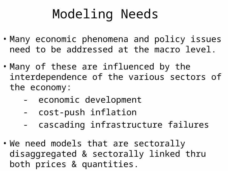
Modeling Needs

• Many economic phenomena and policy issues need to be addressed at the macro level.

• Many of these are influenced by the interdependence of the various sectors of the economy:

- economic development

- cost-push inflation

- cascading infrastructure failures

• We need models that are sectorally disaggregated & sectorally linked thru both prices & quantities.

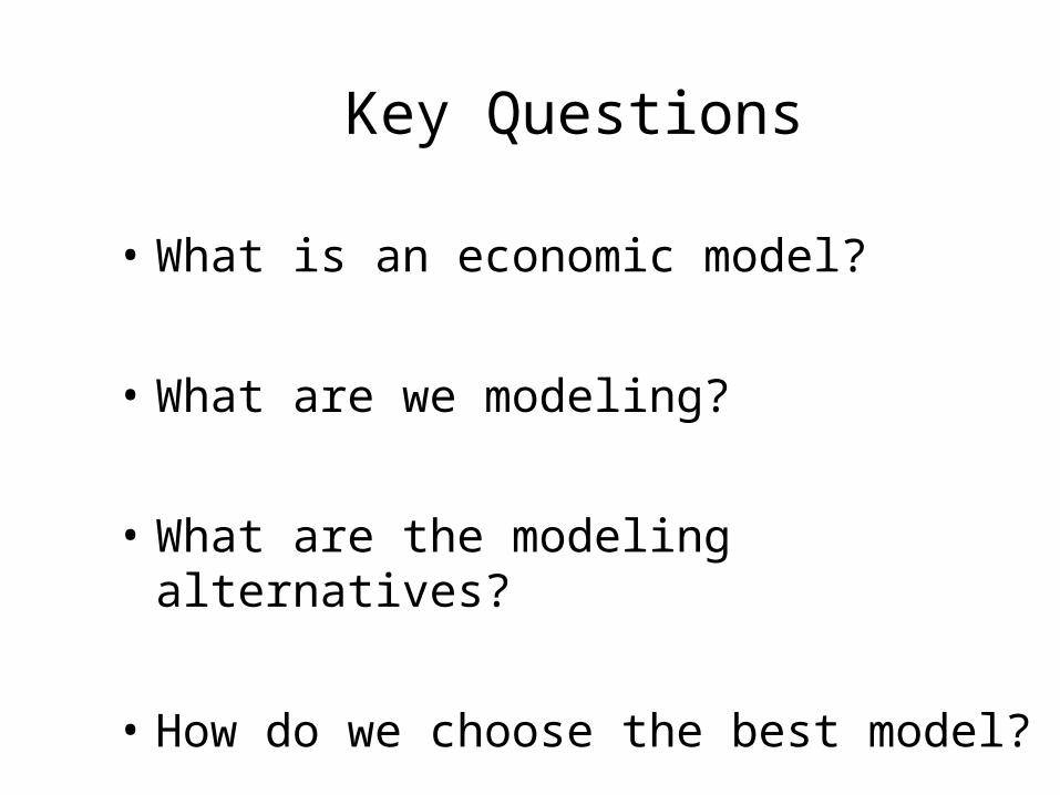
Key Questions

• What is an economic model?

• What are we modeling?

• What are the modeling alternatives?

• How do we choose the best model?

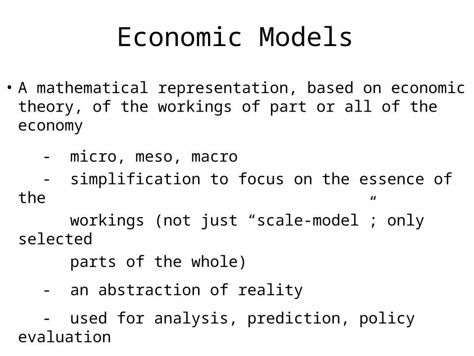
Economic Models

• A mathematical representation, based on economic theory, of the workings of part or all of the economy

- micro, meso, macro

- simplification to focus on the essence of the

workings (not just “scale-model”; only selected

parts of the whole)

- an abstraction of reality

- used for analysis, prediction, policy evaluation

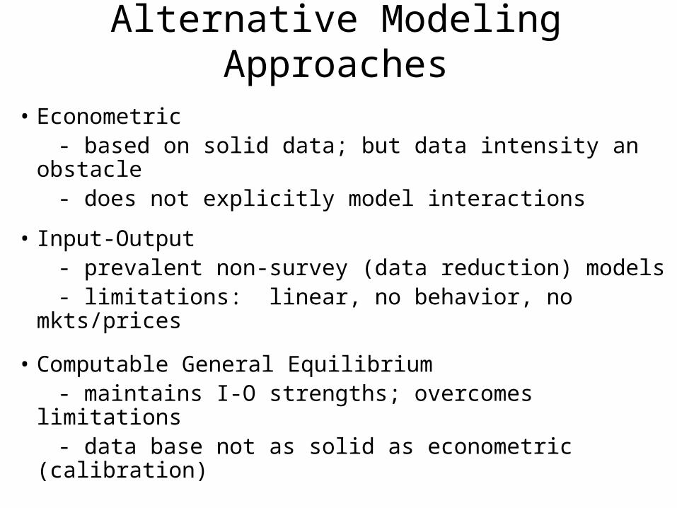
Alternative Modeling Approaches

• Econometric - based on solid data; but data intensity an obstacle - does not explicitly model interactions

• Input-Output - prevalent non-survey (data reduction) models - limitations: linear, no behavior, no mkts/prices

• Computable General Equilibrium - maintains I-O strengths; overcomes limitations - data base not as solid as econometric (calibration)

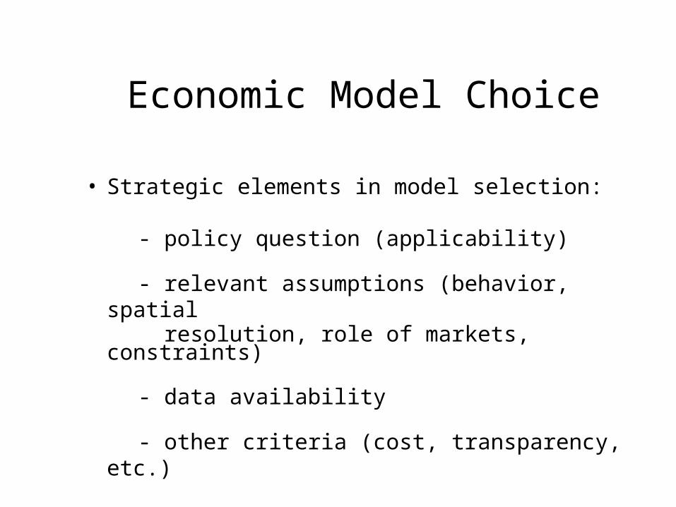
Economic Model Choice

• Strategic elements in model selection:

- policy question (applicability)

- relevant assumptions (behavior, spatial resolution, role of markets, constraints)

- data availability

- other criteria (cost, transparency, etc.)

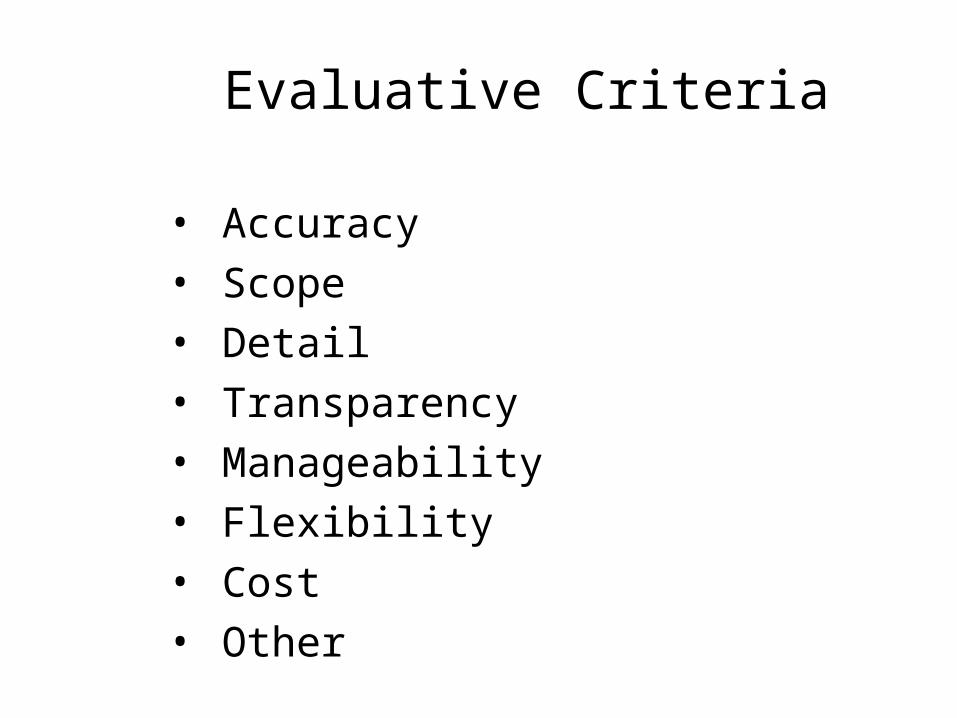
Evaluative Criteria

• Accuracy

• Scope

• Detail

• Transparency

• Manageability

• Flexibility

• Cost

• Other

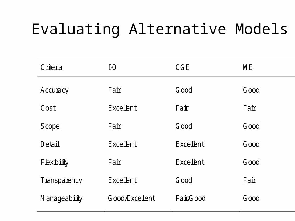
Evaluating Alternative Models

Criteria I-O CGE ME Accuracy Fair Good Good Cost Excellent Fair Fair Scope Fair Good Good Detail Excellent Excellent Good Flexibility Fair Excellent Good Transparency Excellent Good Fair Manageability Good/Excellent Fair/Good Good

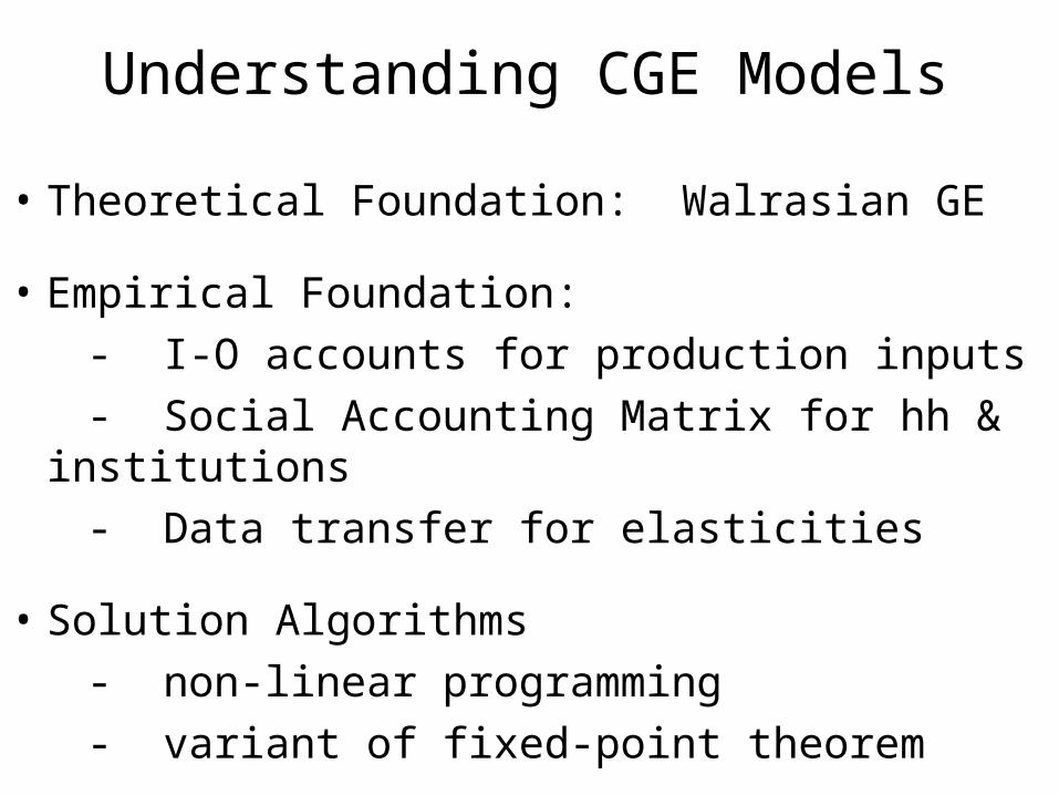
Understanding CGE Models

• Theoretical Foundation: Walrasian GE

• Empirical Foundation:

- I-O accounts for production inputs

- Social Accounting Matrix for hh & institutions

- Data transfer for elasticities

• Solution Algorithms

- non-linear programming

- variant of fixed-point theorem

Overview of CGE

• State-of-the-art impact analysis method

• Relative advantages

- workings of markets & prices

- behavior of individual decision-makers

- substitution & other non-linearities

- ability to accommodate engineering data

• Some disadvantages being overcome

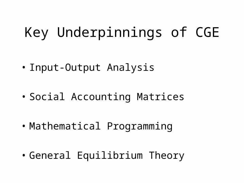
Key Underpinnings of CGE

• Input-Output Analysis

• Social Accounting Matrices

• Mathematical Programming

• General Equilibrium Theory

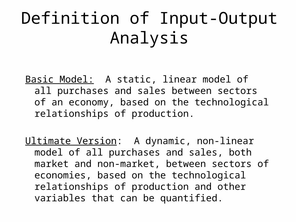
Definition of Input-Output Analysis

Basic Model: A static, linear model of all purchases and sales between sectors of an economy, based on the technological relationships of production.

Ultimate Version: A dynamic, non-linear model of all purchases and sales, both market and non-market, between sectors of economies, based on the technological relationships of production and other variables that can be quantified.

Input-Output Analysis--Rich History

• Worthy of Nobel Prize to Wassily Leontief

• Wealth of empirical data

• Still major tool of impact analysis

• Many superior applications

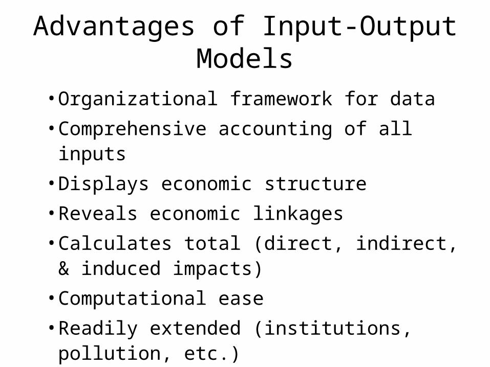
Advantages of Input-Output Models

• Organizational framework for data

• Comprehensive accounting of all inputs

• Displays economic structure

• Reveals economic linkages

• Calculates total (direct, indirect, & induced impacts)

• Computational ease

• Readily extended (institutions, pollution, etc.)

• Can accommodate engineering data

• Empirical models readily available

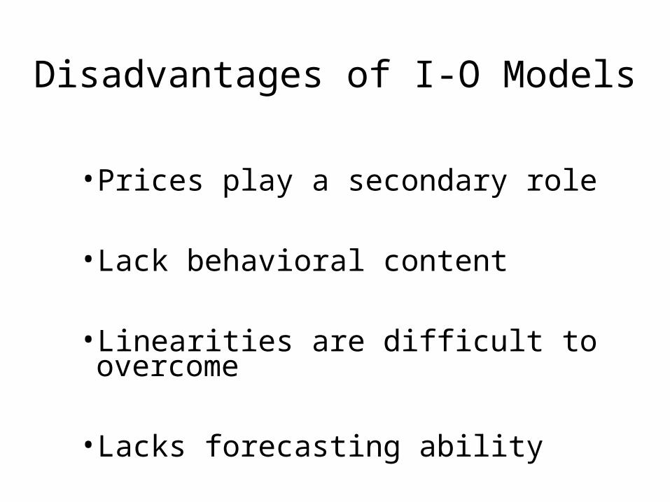
Disadvantages of I-O Models

• Prices play a secondary role

• Lack behavioral content

• Linearities are difficult to overcome

• Lacks forecasting ability

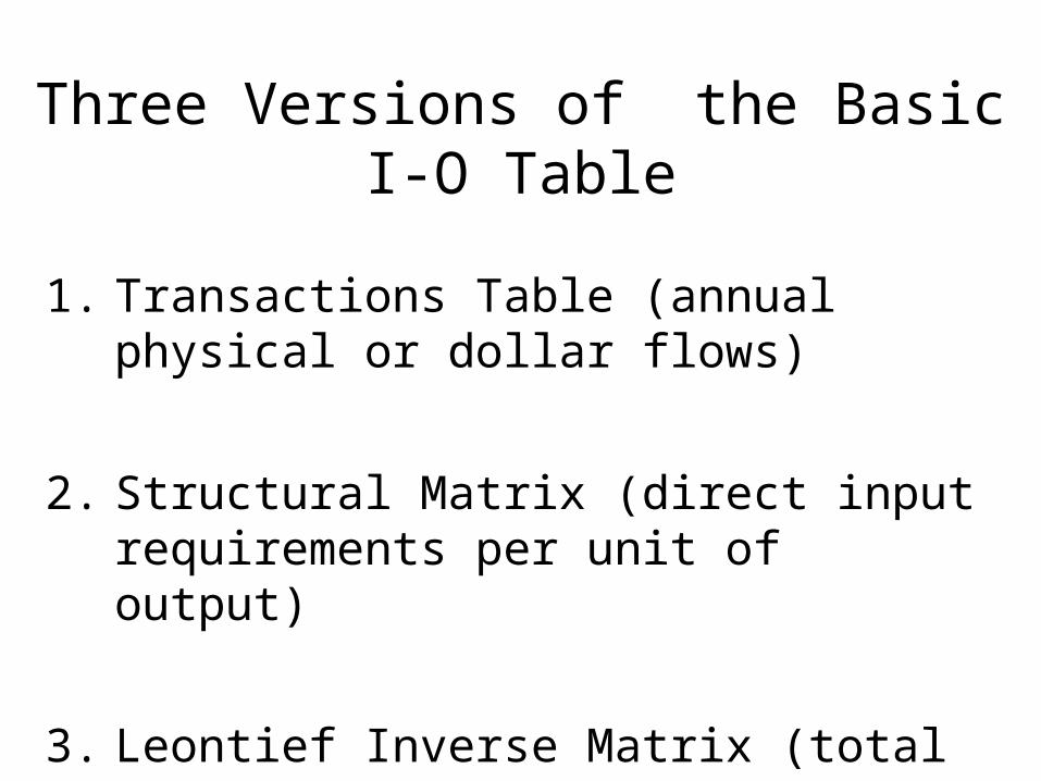
Three Versions of the Basic I-O Table

1. Transactions Table (annual physical or dollar flows)

2. Structural Matrix (direct input requirements per unit of output)

3. Leontief Inverse Matrix (total input requirements per unit of output)

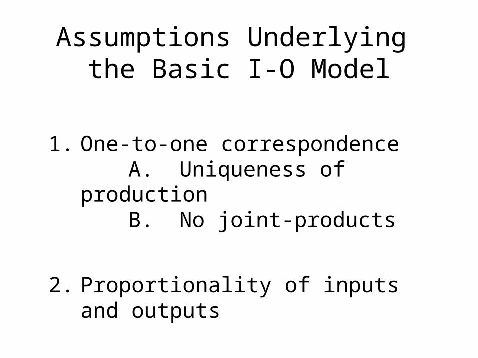
Assumptions Underlying the Basic I-O Model

1. One-to-one correspondenceA. Uniqueness of productionB. No joint-products

2. Proportionality of inputs and outputs

3. No externalities

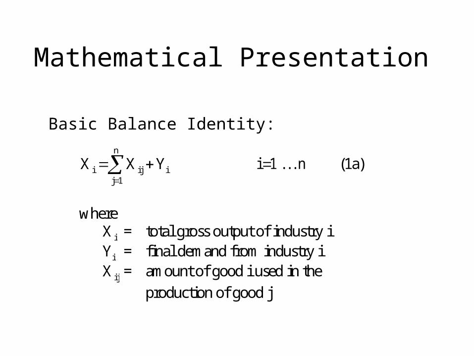
Mathematical Presentation

Basic Balance Identity:

n

i ij ij 1

X X Y

i 1 . . . n (1a)

where

iX = total gross output of industry i

iY = final demand from industry i

ijX = amount of good i used in the

production of good j

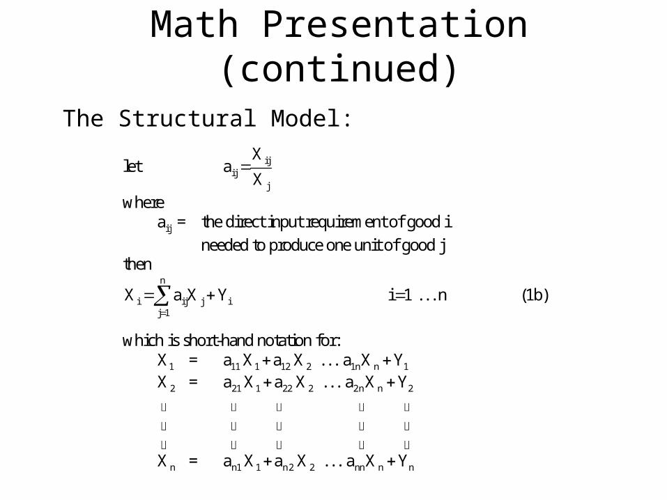
Math Presentation (continued)

The Structural Model:

let ijij

j

Xa

X

where ija = the direct input requirement of good i

needed to produce one unit of good j then

n

i ij j ij 1

X a X Y

i 1 . . . n (1b)

which is short-hand notation for:

1X = 11 1 12 2 1n n 1a X a X . . . a X Y

2X = 21 1 22 2 2n n 2a X a X . . . a X Y

nX = n1 1 n2 2 nn n na X a X . . . a X Y

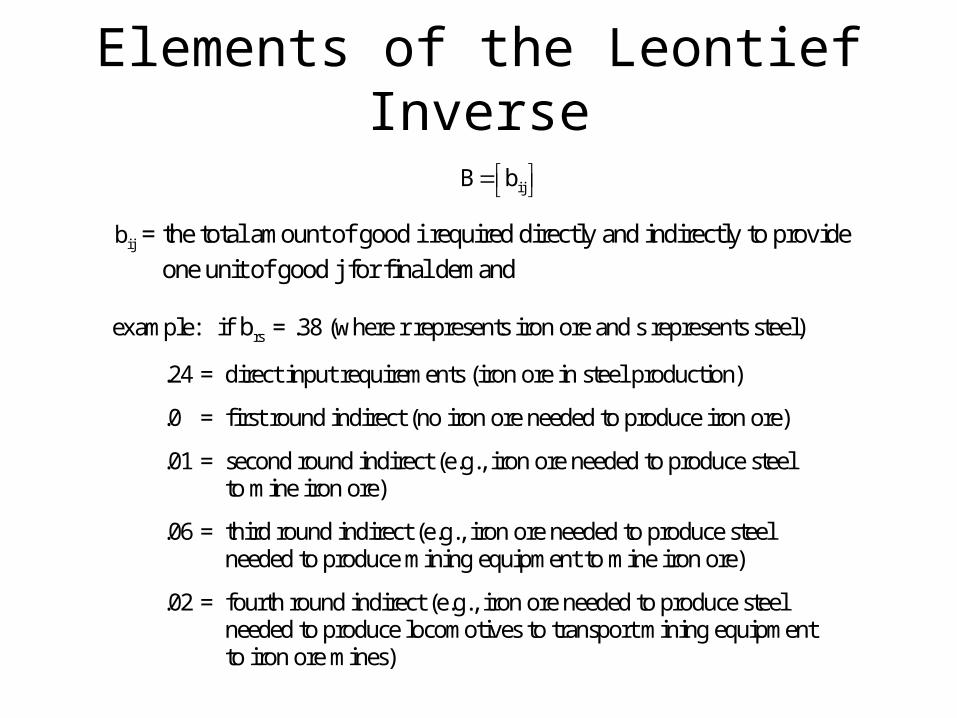
Elements of the Leontief Inverse

ijB b

ijb = the total amount of good i required directly and indirectly to provide

one unit of good j for final demand example: if rsb = .38 (where r represents iron ore and s represents steel)

.24 = direct input requirements (iron ore in steel production)

.0 = first round indirect (no iron ore needed to produce iron ore)

.01 = second round indirect (e.g., iron ore needed to produce steel to mine iron ore)

.06 = third round indirect (e.g., iron ore needed to produce steel needed to produce mining equipment to mine iron ore)

.02 = fourth round indirect (e.g., iron ore needed to produce steel needed to produce locomotives to transport mining equipment to iron ore mines)

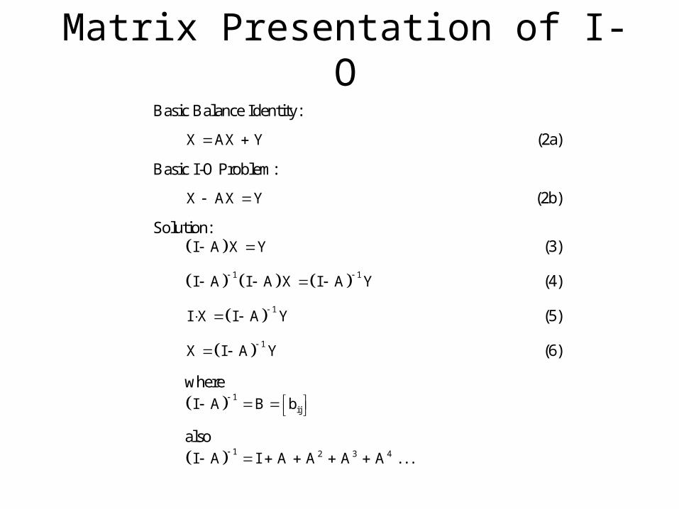
Matrix Presentation of I-O

Basic Balance Identity:

X AX Y (2a)

Basic I-O Problem:

X AX Y (2b)

Solution: I A X Y (3)

1 1I A I A X I A Y

(4)

1I X I A Y

(5)

1X I A Y

(6)

where 1

ijI A B b

also 1 2 3 4I A I A A A A . . .

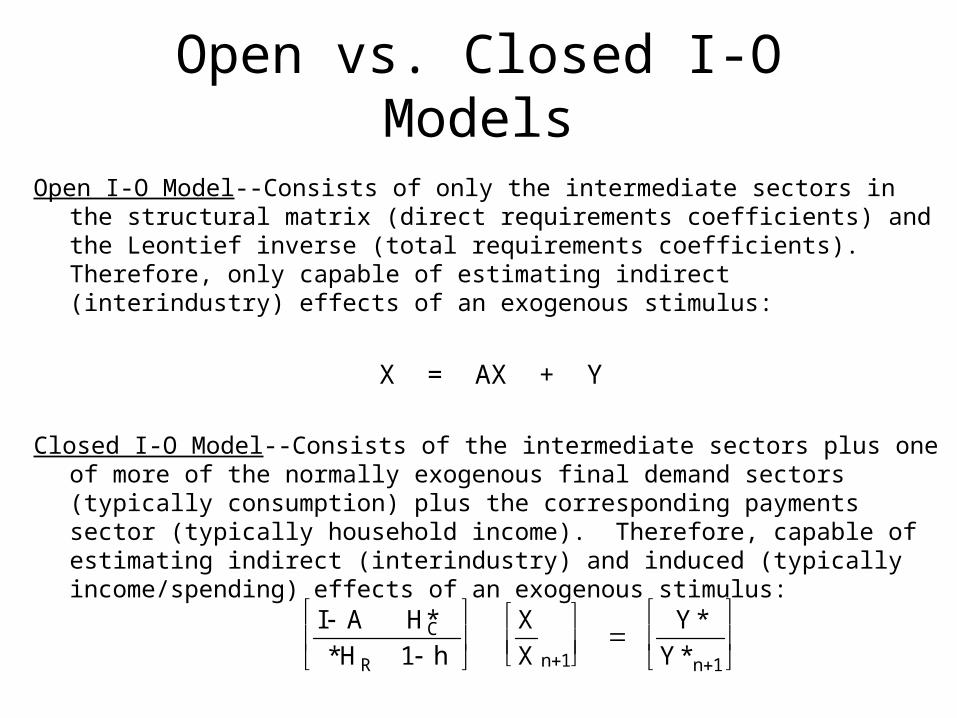
Open vs. Closed I-O Models

Open I-O Model--Consists of only the intermediate sectors in the structural matrix (direct requirements coefficients) and the Leontief inverse (total requirements coefficients). Therefore, only capable of estimating indirect (interindustry) effects of an exogenous stimulus:

X = AX + Y

Closed I-O Model--Consists of the intermediate sectors plus one of more of the normally exogenous final demand sectors (typically consumption) plus the corresponding payments sector (typically household income). Therefore, capable of estimating indirect (interindustry) and induced (typically income/spending) effects of an exogenous stimulus:

I A * HC

*HR 1 h

X

X n1

Y*

Y*n1

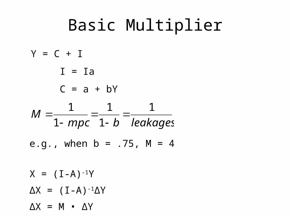
Basic Multiplier

Y = C + I

I = Ia

C = a + bY

leakagesbmpcM

1

1

1

1

1

e.g., when b = .75, M = 4

X = (I-A)-1Y

∆X = (I-A)-1∆Y

∆X = M • ∆Y

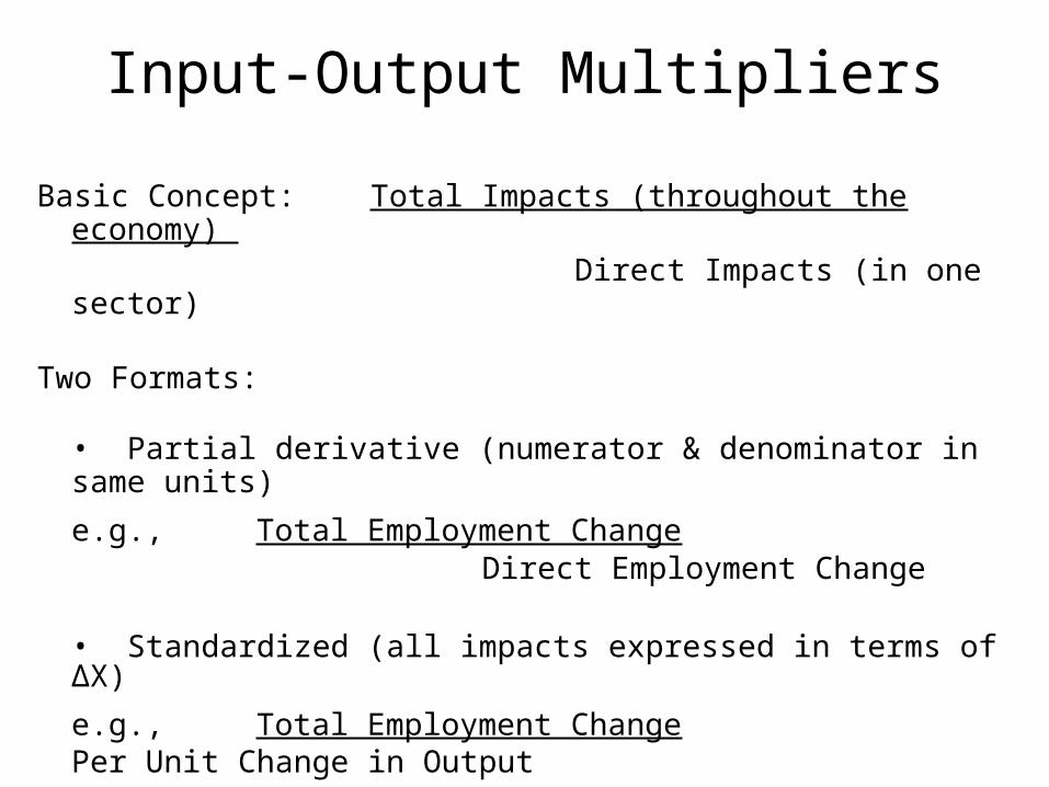
Input-Output Multipliers

Basic Concept: Total Impacts (throughout the economy) Direct Impacts (in one sector)

Two Formats:

• Partial derivative (numerator & denominator in same units)

e.g., Total Employment Change Direct Employment Change

• Standardized (all impacts expressed in terms of ∆X)

e.g., Total Employment ChangePer Unit Change in Output

Multiplier Types

Type I: Total impacts include direct & indirect effects (computed with the open I-O Table)

Type II: Total impacts include direct, indirect & induced (computed with the closed I-O Table)

Type III: Total impacts include direct, indirect & induced (computed with closed Table & marginal consumption

coefficients rather than average coefficients)

Type X: Closed to other elements of Final Demand (e.g., closed w/ respect to investment: dynamic multiplier)

Type SAM: Total impacts with interaction among institutions (computed with Social Accounting Matrix)

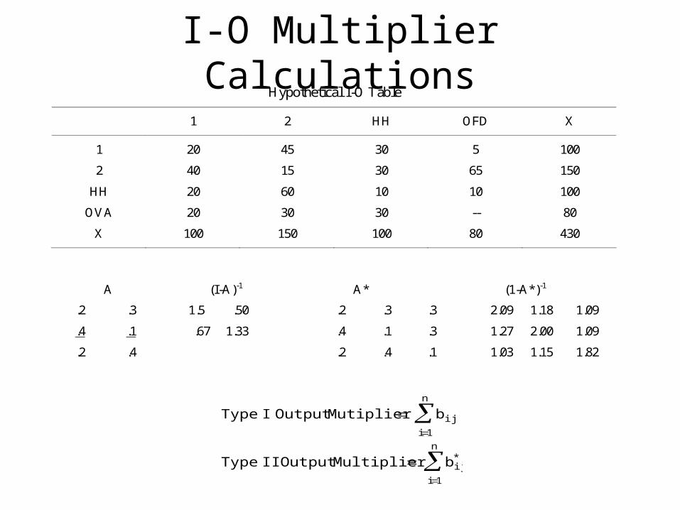
I-O Multiplier Calculations

Type I Output Mutiplier b ij

i1

n

Type II Output Multiplier b ij*

i1

n

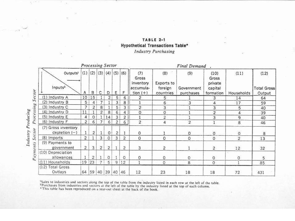
Hypothetical I-O Table

1 2 HH OFD X 1 20 45 30 5 100

2 40 15 30 65 150

HH 20 60 10 10 100

OVA 20 30 30 -- 80

X 100 150 100 80 430

A (I-A)-1 A* (1-A*)-1

.2 .3 1.5 .50 .2 .3 .3 2.09 1.18 1.09

.4 .1 .67 1.33 .4 .1 .3 1.27 2.00 1.09

.2 .4 .2 .4 .1 1.03 1.15 1.82

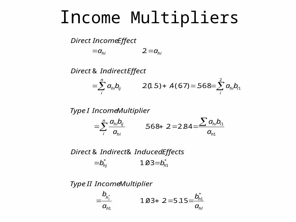
Income Multipliers

hl

h

h

h

hhj

h

ihin

i hi

ijhi

n

i iihiijhi

hihi

a

b

a

b

MultiplierIncomeIIType

bb

EffectsInducedIndirectDirect

a

ba

a

ba

MultiplierIncomeIType

baba

EffectIndirectDirect

aa

EffectIncomeDirect

j

*1

1

*1

*

1

1

2

1

15.5 2. 03.1

03.1

& &

84.2 2. 568.

568. )67(.4. )5.1(2.

&

2.

*

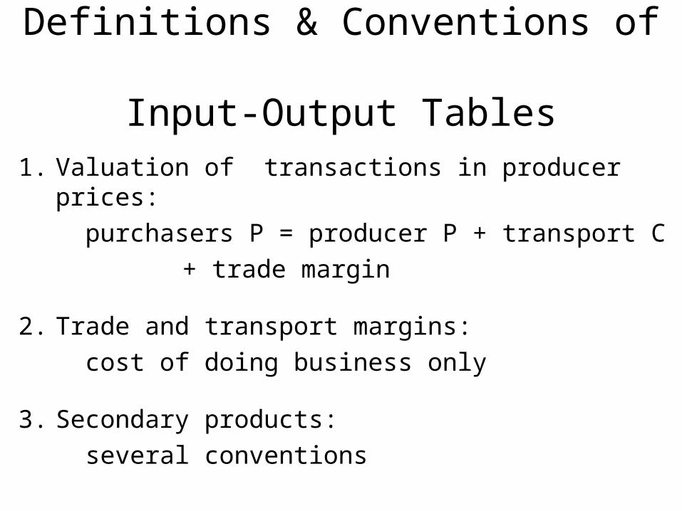
Definitions & Conventions of Input-Output Tables

1. Valuation of transactions in producer prices:

purchasers P = producer P + transport C

+ trade margin

2. Trade and transport margins:

cost of doing business only

3. Secondary products:

several conventions

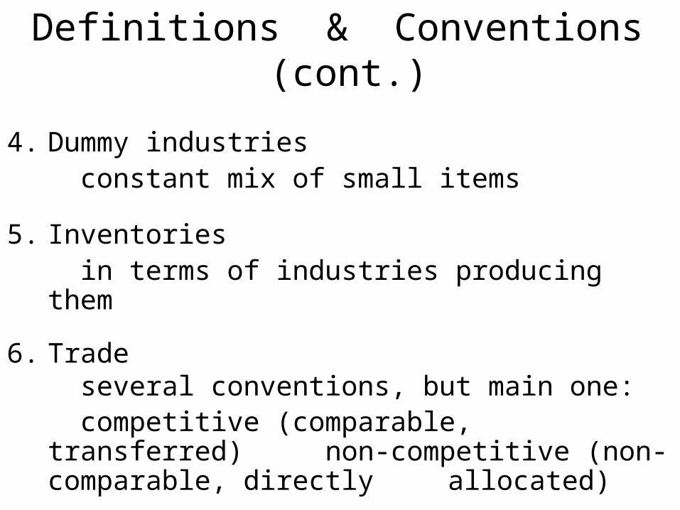
Definitions & Conventions (cont.)

4. Dummy industries constant mix of small items

5. Inventories in terms of industries producing them

6. Trade several conventions, but main one: competitive (comparable, transferred) non-competitive (non-comparable, directly

allocated)

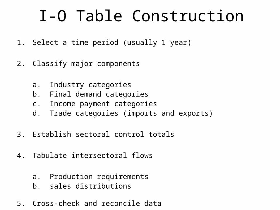
I-O Table Construction

1. Select a time period (usually 1 year)

2. Classify major components

a. Industry categoriesb. Final demand categoriesc. Income payment categoriesd. Trade categories (imports and exports)

3. Establish sectoral control totals

4. Tabulate intersectoral flows

a. Production requirementsb. sales distributions

5. Cross-check and reconcile data

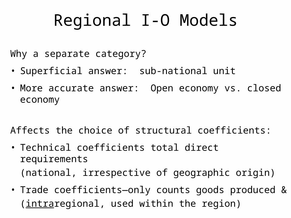
Regional I-O Models

Why a separate category?

• Superficial answer: sub-national unit

• More accurate answer: Open economy vs. closed economy

Affects the choice of structural coefficients:

• Technical coefficients total direct requirements

(national, irrespective of geographic origin)

• Trade coefficients—only counts goods produced &

(intraregional, used within the region)

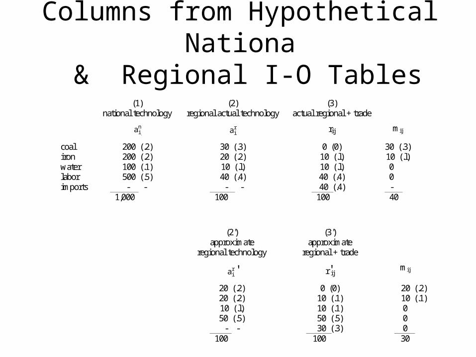
Columns from Hypothetical Nationa & Regional I-O Tables

(1) national technology

(2) regional actual technology

(3) actual regional + trade

a ijn

aijr rij mij

coal 200 (.2) 30 (.3) 0 (0) 30 (.3) iron 200 (.2) 20 (.2) 10 (.l) 10 (.l) water 100 (.1) 10 (.l) 10 (.l) 0 labor 500 (.5) 40 (.4) 40 (.4) 0 imports - - - - 40 (.4) - 1,000 100 100 40

(2')

approximate regional technology

(3') approximate

regional + trade

aijr ' r'ij mij

20 (.2) 0 (0) 20 (.2) 20 (.2) 10 (.1) 10 (.1) 10 (.l) 10 (.1) 0 50 (.5) 50 (.5) 0

- - 30 (.3) 0 100 100 30

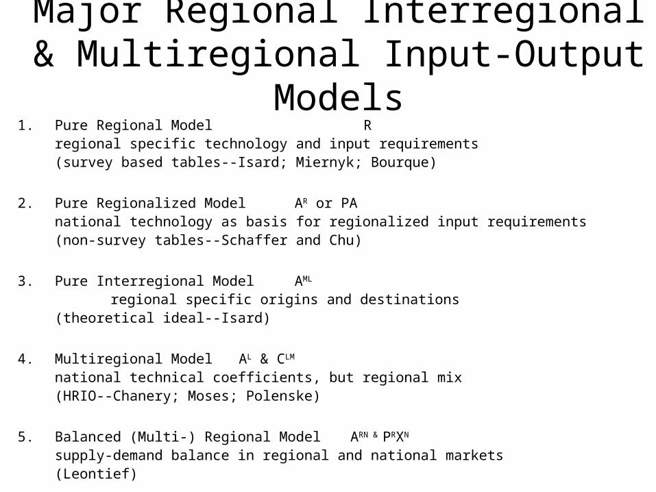
Major Regional Interregional & Multiregional Input-Output Models

1. Pure Regional Model Rregional specific technology and input requirements(survey based tables--Isard; Miernyk; Bourque)

2. Pure Regionalized Model AR or PAnational technology as basis for regionalized input requirements(non-survey tables--Schaffer and Chu)

3. Pure Interregional Model AML

regional specific origins and destinations(theoretical ideal--Isard)

4. Multiregional Model AL & CLM

national technical coefficients, but regional mix(HRIO--Chanery; Moses; Polenske)

5. Balanced (Multi-) Regional Model ARN & PRXN

supply-demand balance in regional and national markets(Leontief)

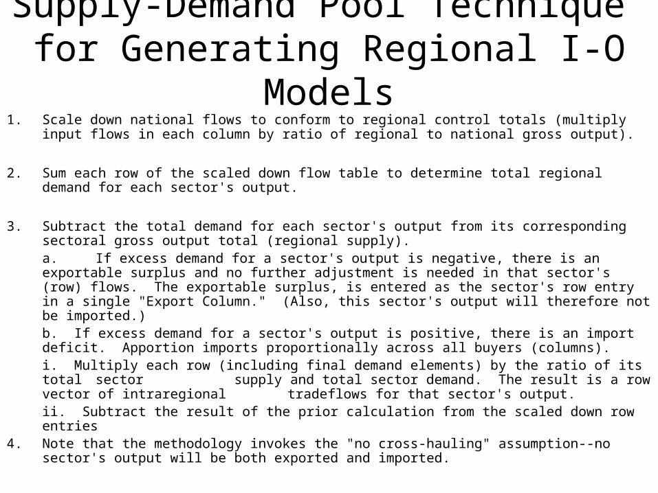
Supply-Demand Pool Technique for Generating Regional I-O Models

1. Scale down national flows to conform to regional control totals (multiply input flows in each column by ratio of regional to national gross output).

2. Sum each row of the scaled down flow table to determine total regional demand for each sector's output.

3. Subtract the total demand for each sector's output from its corresponding sectoral gross output total (regional supply). a. If excess demand for a sector's output is negative, there is an exportable surplus and no further adjustment is needed in that sector's (row) flows. The exportable surplus, is entered as the sector's row entry in a single "Export Column." (Also, this sector's output will therefore not be imported.)b. If excess demand for a sector's output is positive, there is an import deficit. Apportion imports proportionally across all buyers (columns).

i. Multiply each row (including final demand elements) by the ratio of its total sector supply and total sector demand. The result is a row vector of intraregional tradeflows for that sector's output. ii. Subtract the result of the prior calculation from the scaled down row entries

4. Note that the methodology invokes the "no cross-hauling" assumption--no sector's output will be both exported and imported.