A characterization of computable analysis on unbounded ...

A characterization of computable analysis onunbounded domains using differential equations

Manuel L. Campagnoloa,1, Kerry Ojakian∗,b,2

aGrupo de MatematicaDepartamento de Ciencias e Engenharia de Biossistemas

Instituto Superior de AgronomiaTapada da Ajuda, 1349-017 Lisboa, Portugal

bDepartment of Mathematics and Computer ScienceSaint Joseph’s College

155 West Roe BoulevardPatchogue, NY 11772Phone: 631-687-2616

Fax: 631-758-5997

Abstract

The functions of computable analysis are defined by enhancing normal Tur-ing machines to deal with real number inputs. We consider characterizationsof these functions using function algebras, known as real recursive functions.Since there are numerous incompatible models of computation over the reals,it is interesting to find that the two very different models we consider can beset up to yield exactly the same functions. Bournez and Hainry [6] used afunction algebra to characterize computable analysis, restricted to the twicecontinuously differentiable functions with compact domains. In our paper [11],we found a different (and apparently more natural) function algebra that alsoyields computable analysis, with the same restriction. In this paper we improveour result in [11], finding three function algebras characterizing computableanalysis, removing the restriction to twice continuously differentiable functionsand allowing unbounded domains. One of these function algebras is built uponthe widely studied real primitive recursive functions. Furthermore, the proof ofthis paper uses our method of approximation from [12], whose applicability isfurther evidenced by this paper.

Key words: computable analysis, real recursive functions, function algebras,analog computation, differential equations

∗Corresponding authorEmail addresses: [email protected] (Manuel L. Campagnolo),

[email protected] (Kerry Ojakian)1Forest Research Center, ISA, Technical University of Lisbon, and SQIG, Instituto de

Telecomunicacoes, Lisboa2Department of Mathematics and Computer Science, Saint Joseph’s College

Preprint submitted to Elsevier March 29, 2011

1. Introduction

When is a function over the reals computable? The answer to this ques-tion when working over the naturals has a generally agreed upon answer (e.g.Turing-computability, recursive, etc.), but over the reals, there are a number ofincompatible computational models. We can make an informal categorization ofthese models: 1) Models that evolve in discrete time steps, and 2) Models thatevolve in continuous-time. In the first category we have models like computableanalysis [23] [29], Grzegorczyk’s algebras of functionals [20], BSS-machines [2][1], real random access machines [27] [8], and a recursive characterization ofcomputable real functions [7]. In the second category, we have models likeShannon’s circuit model (the General Purpose Analog Computer) [28] [18], con-tinuous neural networks [24], and Moore’s real recursive functions [25] (for anup-to-date review of continuous-time models see [3]). Discrete-time models typ-ically use some abstract machine, like a Turing machine, where there is a clearnotion of the “next state” within a computation. Continuous-time models typ-ically use differential equations to describe a computation which can be viewedas proceeding continuously in real time, with no clear notion of “next state.”The dissimilarity of the models makes it interesting to investigate connectionsbetween them, as a number of recent papers have done. It is known that sev-eral approaches to computability over the real numbers coincide: In particular,computable analysis, computable functionals [20], and continuous domains [17]all yield the same class of functions. Here, we are most interested in comparingcomputable analysis with continuous-time models. Bournez et. al. [4] charac-terize computable analysis with General Purpose Analog Computers. Bournezand Hainry [5] [6] partially characterize computable analysis with real recursivefunctions. We continue in this direction, providing various characterizations ofcomputable analysis with real recursive functions. Finding different models forthe same set of functions could be useful from a technical point of view, allowingone to prove facts about one model by using one of its characterizations. Fur-thermore, understanding when models of computation over the reals agree anddisagree should be vital for a deeper perspective on what we mean by computingover the reals.

Computable analysis seeks to give a realistic account of how a digital com-puter calculates with real numbers: A function is computable if from approxi-mations to the input, we can approximate the output (using a standard discrete-time Turing machine). Moore’s real recursive functions is a generic name weuse for models based on function algebras over the reals, i.e. a specific set ofbasic functions are closed under a specific set of operations, some involving dif-ferential equations (for background see Moore’s original paper [25], along withthe clarifying papers [15] and [22]). Moore’s motivation was to develop an ana-log version of the normal recursive functions over the naturals, replacing therecursion operation with a differential equation operation. The main result ofthis paper (theorem 2.17) characterizes the functions of computable analysis viareal recursive functions, using three different function algebras.

Bournez and Hainry [6] proposed a class of real recursive functions that

2

partially captured computable analysis. In particular, their function algebracharacterizes the twice continuously differentiable (C2) functions with compactdomain. Our function algebras remove the restriction to C2 and compact do-mains. Their function algebra contains a set of basic functions and is closedunder the following operations: Composition, linear integration, a limit opera-tion and a root-finding operation. One of our characterizations will be similar,and another one will replace the root-finding operation with an operation thatfinds the inverse of a function. The third, and most interesting function al-gebra, does not have a root-finding operation or inverse operation, but insteadstrengthens the operation of integration, removing the linearity restriction. Thisthird characterization (called ODE?

k(LIM)) of computable analysis appears tobe about as natural as one could hope for (using real recursive functions); itsunderlying functions (before a kind of limit operation is applied) are merely afew basic functions, along with functions that can be built from these, usingdifferential equations. In fact, this function algebra is very similar to the realprimitive recursive functions, which have been studied by a number of authors(e.g. [15], [22], [6]; note that there are slight differences between their definitionsand only [22] actually uses the name “real primitive recursive functions”).

In addition to providing new characterizations which apply to all of the func-tions of computable analysis, our proofs use our method of approximation (de-veloped in [12]). To capture computable analysis with an analog model, earlierapproaches have proceeded by fixing a particular characterization of computableanalysis, and then exploiting its particular properties in order to simulate itsoperation in the analog model (e.g. Turing machines are used in [4], and com-putable functionals are used by Bournez and Hainry [6]). While we of coursebegin with some model of computable analysis (we choose oracle Turing ma-chines), we convert the problem into a question about function algebras, andare no longer explicitly concerned with computable analysis. In particular, weintroduce the notion of one class of functions approximating another one, andreduce the work to proving a series of approximations. Our approach offers anumber of advantages. Due to the transitivity of the approximation relation,we can break up the proof into a number of natural steps. The approximationcontext works naturally with the inductive structure of the function algebras.And finally, our approach seems to be more general, facilitating reasoning aboutour problem and other problems of this kind. The significance of the method ofapproximation is discussed in more detail in the conclusion (section 5).

Section 2 introduces the terminology and discusses the main result. Section 3outlines our proof, breaking it up into a minor step and a major step. The minorstep follows directly from our work in [11], and thus we simply summarize theideas for this step. The major step is set up in section 3 (page 10), leavingthe technical details of this step for section 4 (page 20). In section 5 (page 41)we reflect on the significance of our approach to this problem, comparing it toother approaches, and also consider strengthening our result by simplifying ourfunction algebra. There is an index at the end of the paper.

3

2. Formulating the Main Result

We now provide the basic definitions and state the result, leaving the prooffor the next section.

Definition 2.1. For us, unless stated otherwise, a function will always havedomain D ⊆ Rk and codomain R. To indicate that a function f is defined on allof D, with codomain E, we write f : D → E. By “domf” we mean the domainof f . If f : Dk → E and X ⊆ D, we write f|X for the restriction of f to the

domain Xk.

Typical domains in this paper are: The naturals N = {0, 1, 2, . . .}, the integersZ = {. . . ,−1, 0, 1, . . .}, the rationals Q, and the reals R.

Definition 2.2. For x = (x1, . . . , xk), and X ⊆ R, we write x ∈ X to meanthat each xi is in X; for a unary function f , the vector (f(x1), . . . , f(xk)) isabbreviated by f(x).

One of the models we will consider is computable analysis, also known astype-2 computability (see [23] or [29] for details). A function f : R → R iscomputable in the sense of computable analysis if there is an oracle Turingmachine, which on input n (which we call the accuracy input), using an oraclefor x ∈ R, outputs a rational within 1/n of f(x). The oracle is used as follows: Ifthe machine writes a number m on the oracle tape, it receives a rational within1/m of x. The following definition generalizes this discussion to functions withdomain Rk.

Definition 2.3. We say a function f : Rk → R is in CR iff it is computable inthe sense of computable analysis.

It is common in computable analysis to restrict the domain to bounded intervals;however the functions of CR are defined on unbounded domains.

We now turn our attention to function algebras. We use the term operationto refer to an operator that maps a finite number of functions to a single function.Some operations are partial, meaning that they are undefined given certainfunctions as arguments. The next few pages of technical definitions will befollowed by some (hopefully) helpful examples.

Definition 2.4. Suppose B is a set of functions (called basic functions), andO is a set of operations. Then FA[B;O] is called a function algebra, and itdenotes the smallest set of functions containing B and closed under the oper-ations in O. For ease of readability, we display the elements of B and O ascomma separated lists.

Some of the most important operations will be defined using differentialequations. From a vector valued function g = (g1, . . . , gk) we can form aninitial value problem (IVP) in parameters a = (a1, . . . , ak), given by thefollowing system of equations:

(h)′ = g(a, h) , h(0, a) = a.

4

We can also write the same system of equations more explicitly as follows:

∂∂xh1(x, a) = g1(a, h1, . . . , hk)

...∂∂xhk(x, a) = gk(a, h1, . . . , hk)

,

h1(0, a) = a1

...hk(0, a) = ak

(1)

We understand the vector a to be parameter variables, as opposed to just fixedreals; thus we write the solution h = (h1, . . . , hk) with the parameter variablesa as arguments (i.e. exactly the situation described in [21], p. 93).

In general, one IVP can have many distinct solutions; when we use an IVPto define an operation below, we want to avoid this case. Roughly, we will sayan IVP is well-posed if it has a unique solution, though more precisely, we meanthe following.

Definition 2.5. Consider the IVP (1).

• h(x, a) is a maximal solution with domain D if h is a solution on someopen set D ⊆ Rk+1, and for any open set E (such that D ( E), there isno solution to the IVP on E.

• The IVP is well-posed if there is a unique maximal solution.

We can now define the operations we will be using (note that in the opera-tions there is an implicit choice of which arguments of the function we chooseto use; any choice is allowed). Strictly speaking, all the following operations arepartial. In the operations, conditions are described that need to be satisfied inorder for the operation to output a function. If any condition is not satisfied bythe input functions, then the operation is undefined for that input.

Definition 2.6. (Operations for real functions)

1. The operation ODE takes as input, functions g1, . . . , gk. It is defined if theIVP given by the gi is well-posed. Otherwise the operation is undefined.If the operation is defined, the IVP has a solution h = (h1, . . . , hk) withdomain D as described in definition 2.5. The operation outputs h1 anddom h1 = D.

2. LI is the same as ODE, with the additional condition that the g are linearin the h.

3. Let comp be the composition operation. The operation comp takes as in-put, functions f, g1, . . . , gk. It is defined if the functions f and gi haveappropriate arities; otherwise it is undefined. When defined, it is as fol-lows. Given

f(y1, . . . , yk), g1(x1, . . . , xm), . . . , gk(x1, . . . , xm),

it returns the simultaneous composition:

h(x1, . . . , xm) = f(g1(x1, . . . , xm), . . . , gk(x1, . . . , xm)),

which is defined on the maximal well-defined domain, i.e.

dom h = {x ∈ Rm : x ∈ dom g and g(x) ∈ domf}.

5

4. The operation Inverse receives a function f(x, a) : R × Rk → R as input.The operation Inverse is defined on f if:

(a) For all real a, f(x, a) is a bijection (of R) in x, and(b) For all real a and x, ∂

∂xf(x, a) exists and is positive.

Otherwise it is undefined. If Inverse is defined on f then it returns f−1 :R × Rk → R, the inverse in x, i.e. f(f−1(x, a), a) = x = f−1(f(x, a), a)(f−1 may be referred to as Inverse(f, x); the “x” indicates the variable off to which Inverse is applied).

5. The root-finding operation UMU (“ unique µ”) receives a function f(x, a) :R× Rk → R as input. The operation UMU is defined on f if:

(a) For all real a, f(x, a) is increasing in x (not necessarily strictly), and(b) For all real a, there is a unique x such that f(x, a) = 0 (and at that

x, ∂∂xf exists and is positive).

Otherwise it is undefined. If UMU is defined on f , it returns the functiong : Rk → R such that for a ∈ Rk, g(a) is the unique x such that f(x, a) = 0(g may be referred to as UMU(f, x); the “x” indicates the variable of f towhich UMU is applied).

Our most important operation, ODE (also called differential recursion byother authors) is defined without analysis style conditions such as requiring thegi be continuous, Lipschitz, etc. In doing so, our definition is similar to [22,Def. 3.5], rather than to that of [15]. However, as we shall see in lemma 2.15,whenever we actually use the ODE operation, all the functions involved willbe smooth (i.e. Cn for some n ≥ 1, as defined below). Thus, whether ourODE operation is defined as in [22] or with the requirement of being locallyLipschitz as in [15], our results remain the same. Furthermore, the two classes offunctions we define with ODE (ODEk and ODE?

k; see definition 2.10) are bothclosed under composition, so we can use standard manipulations on differentialequations to derive the following more flexible looking operation:

On input f and g, the derived operation operates just like ODE,except that the IVP it solves is the following:

(h)′ = g(x, a, h) , h(0, a) = f(a)

(i.e. in the earlier system (1), we can replace each initial condition“hi(0, a) = ai” by “hi(0, a) = fi(a)” and allow the system to benon-autonomous, i.e. allow x as an input to g).

Definition 2.7. We say that f is Cn if f has continuous partial derivatives ofall order k ≤ n, on its domain.

The following well known result (see [21], chapter V, theorem 3.1 and corollary4.1, and chapter II, theorem 3.1) will be central to prove lemma 2.15. In par-ticular, this proposition shows that if the gi are Cn then the corresponding IVPis well-posed.

6

Proposition 2.8. Consider the IVP

(h)′ = g(a, h) , h(0) = a,

and suppose n ≥ 1. If g is Cn and has an open domain, then its unique maximalsolution h(x, a) has an open domain and is Cn.

Among our basic functions, one of the most significant will be a functionwhich indicates if a number is to the left or right of zero. Such a function isthe Heaviside step function: θ(x) = 0 if x < 0 and θ(x) = 1 if x ≥ 0. However,instead we will use a function of this sort, with some smoothness constraint.For integer k ≥ 1, we let

θk(x) =

{0, if x < 0;xk, if x ≥ 0.

Thus, we think of the function θk as a Ck−1 substitute for the Heaviside function.Besides θk we will also have basic functions like the constant function “0” andthe projection functions P (e.g. P contains P(2,1)(x, y) = x, P(3,2)(x, y, z) = y,etc.). We will use the same names for these functions in the context of variousdomains (N, Q, and R).

The rank of a function with respect to an operation counts the number ofnested applications of the operation in the construction of the function.

Definition 2.9. Given a function algebra F = FA[B; op1, . . . , opn,OP], we de-fine the rank of the construction of the a function f in F with respect to theoperation OP:

1. If f is in B (i.e. f is a basic function) then rank(f) = 0.

2. If f is opi(g1, g2, . . .), then rank(f) = max{rank(g1), rank(g2), . . .}.3. If f is OP(g1, g2, . . .) then

rank(f) = 1 + max{rank(g1), rank(g2), . . .}.

We say that f is of rank c if it has a construction of rank less than or equal toc.

Note that by definition, a function of rank c is also of rank n for n ≥ c. We nowdefine the relevant function algebras over the reals.

Definition 2.10. (Function algebras over the reals) Let k ≥ 1 be an inte-ger.

• Let RMUk be FA[0, 1, θk,P; comp, LI,UMU].

• Let RMU(c)k be the functions of RMUk that have rank c with respect to

the operation UMU.

• Let πRMU(c)k be the function algebra RMU

(c)k , with the constant func-

tions −1 and π added as basic functions.

7

• Let INVk be FA[0, 1,−1, θk,P; comp, LI, Inverse].

• Let INV(c)k be the functions of INVk that have rank c with respect to the

operation Inverse.

• Let ODEk be FA[0, 1,−1, θk,P; comp,ODE].

• We define ODE?k as follows: A function f is in ODE?

k iff f is in ODEk

and f has domain Rn for some n.

We now discuss some examples.

Example 2.11. Consider the initial value problem:

∂

∂xh(x, y) = 1 , h(0, y) = y

The unique function satisfying this differential equation is h(x, y) = x+y. Sincethe above function algebras all contain the constant function 1, and are closedunder linear differential equations, they all contain the addition function. (Asan exercise, do multiplication).

The following example shows us a function in ODEk that is not in the otherfunction algebras.

Example 2.12. The non-linear initial value problem

h′ = h2 , h(0) = 1,

defines the function h(y) = 11−y and so 1

x = h(1 − x) is in ODEk, for any

k ≥ 1 (following our conventions, the domain of 1x is (0,+∞), not containing

any non-positive numbers). Note that the linear differential equations of LI donot suffice to define this function.

Since the function 1x is not total (over R), it is not in ODE?

k; for this reasonwe often work with ODEk in the proofs, even though in the end we care aboutODE?

k. The next example uses the power of the basic function θk.

Example 2.13. Campagnolo et. al. [9, lemma 4.7] defined a kind of step func-tion, step : R → R, which is increasing, continuous, and satisfies the followingproperty:

For any u ∈ Z, step(x) = u for x ∈ [u, u+ 1/2].

This construction can be carried out in RMU(c)k , for k ≥ 1, c ≥ 0.

Example 2.14. The constant functions −1 and π can each be constructed in

RMU(1)k . To get −1 we just find the root of x + 1. For π, see the proof of

lemma 5.1 in [6] (in case the reader checks the reference, note that despiteinitial appearances, a single application of UMU suffices to define π).

8

Other examples of functions in all the function algebras are sinx, ex, and theconstant functions q (for any rational q).

We list some basic properties of these function algebras in the next lemma.

Lemma 2.15. (Properties of Function Algebras)

1. πRMU(c)k ⊆ RMU

(c+1)k .

2. Fk ⊆ Fk−1, where Fk is any of the function algebras in definition 2.10containing θk as a basic function, and Fk−1 is the same function algebrawith the basic function θk−1 instead.

3. For every function algebra of definition 2.10, with the exclusion of thefunction algebra ODEk, if f is one of its functions, then the domain of fis Rn for some n.

4. Every function in ODEk has an open domain and is Ck−1, for k ≥ 2.

Proof

Point 1: Follows from example 2.14

Point 2: Follows, since θk(x) = x · θk−1(x), and all the algebras areclosed under multiplication.

Point 3: By R× we mean Rn for some n ≥ 1. The conditions on theinput to Inverse and UMU in fact require the input function to havedomain R×; the output function also has domain R×. Since the basicfunctions have domain R×, and the operations (comp, Inverse, UMU,and LI) all preserve that property whenever they are defined, all the

functions in RMUk, RMU(c)k , πRMU

(c)k , INVk, and INV

(c)k have

domain R×; by definition, the functions of ODE?k have domain R×.

Point 4: The basic functions, and in particular θk, are all Ck−1

and have open domains. To conclude with this point, we just needto check that all the operations preserve these properties. Supposethe function f and the vector-valued function g = (g1, . . . , gn) areCk−1 and have open domains. It is known that the compositionf(g1, . . . , gn) is Ck−1. Suppose the domains of f and g are the opensets F and G, respectively. Then the domain of f(g1, . . . , gn) isG∩g−1(F ), which is open, since the continuity of g implies g−1(F )is open. For the ODE operation, suppose that g1, . . . , gk are in thealgebra. By inductive hypothesis they are Ck−1 and have open do-mains. Therefore, by lemma 2.8 (using the fact that k− 1 ≥ 1), theunique solution output by ODE is Ck−1 and has an open domain.

�

To make the connection to computable analysis, we consider a limit operationwhich allows us to take the limit of a function as some argument goes to infinity,provided the function converges rapidly to its limit, i.e. this is exactly the kindof limit that is implicit in the definitions of computable analysis.

9

Definition 2.16. (Limits)

• The operation LIM takes as input a function f∗(x, t) : Rk × R → R. It isdefined on f∗ if:

1. For all real x, the limit f(x) = limt→∞

f∗(x, t) exists, and

2. For all real t > 0 and all real x, |f(x)− f∗(x, t)| ≤ 1/t.

Otherwise it is undefined. If LIM is defined on f∗ then it returns f(x) :Rk → R (the function f may be referred to as LIM(f∗)).

We will see in definition 3.7, that f∗ is an “approximation” of f .

• Given a class of functions F, we let F(LIM) denote the closure of F underthe operation LIM.

It is easy to check that CR is closed under LIM, i.e. CR = CR(LIM). For all theclasses F considered in this paper, we in fact only need to apply LIM once toany function, i.e. {LIM(h) | h is in F} = F(LIM).

We now state the main theorem, obtaining three characterizations of thetotal computable functions via three function algebras.

Theorem 2.17. For k ≥ 2, CR = ODE?k(LIM) = RMUk(LIM) = INVk(LIM).

We consider the characterization by ODE?k(LIM) the most natural and interest-

ing. In characterizing CR by ODE?k(LIM), we have characterized computable

analysis by a function algebra which differs from the real primitive recursivefunctions in two essential ways: The presence of the limit operation and the pres-ence of the extra basic function θk. The theorem improves the previous resultsof this kind. In our paper [11] we partially characterized CR by ODE?

k(LIM);namely, we only characterized those function of CR which are C2 and have acompact domain. With the same restriction on CR, Bournez and Hainry [6]partially characterized CR by RMUk(LIM), where the operation LI is replacedby a slightly unnatural variant; however, we should note that their result allowsthe limit operation to be interleaved with the other operations of the functionalgebra. In addition to providing a full characterization, we introduce the newcharacterization by INVk(LIM), and our proof uses our method of approxima-tion.

3. The Proof

Since our proof boils down to proving a number of inclusions, we summarizethese inclusions below, making reference to the lemmas which immediately implythem. The first step (the main step) will be discussed in part 3.2. The secondstep (the minor step), discussed in part 3.1, summarizes a series of inclusionsthat follow immediately from the referenced lemmas. The third step simplyputs together the first two steps in order to prove theorem 2.17.

10

1. (The Main Step) Lemma 3.6 will show that for any k ≥ 1, we have:

CR ⊆ πRMU(1)k (LIM).

2. (The Minor Step) The lemmas 2.15, 3.1, 3.2, 3.4, and 3.5 imply thefollowing two chains of inclusions:

• For k ≥ 5 :

πRMU(1)k ⊆ RMU

(2)k ⊆ INV

(2)k ⊆ ODE?

k−2 ⊆ ODE?k−3 ⊆ CR

• For k ≥ 2 :

πRMU(1)k ⊆ RMU

(2)k ⊆ RMUk ⊆ INVk ⊆ CR

3. The theorem 2.17 follows immediately: We arrive at a cycle of inclusions byclosing the classes of step 2 under limits, combining the resulting inclusionswith the inclusion of step 1, and using the fact that CR is closed underlimits.

Our proof in fact also characterizes CR by πRMU(1)k (LIM), RMU

(2)k (LIM) and

INV(2)k (LIM) (all for k ≥ 2), though we only included the cleaner characteriza-

tions in theorem 2.17.

3.1. The Minor Step

The inclusions for the minor step are discussed in this section. The lemmasof this part are taken right from our previous paper [11], though we have (hope-fully) improved the notation in this paper. We use RMU for BH, INV for L,and ODE for G (in the case of BH, it had the extra basic function “−1”, whichwe can remove as per example 2.14). We will discuss the intuitions behind someof the proofs (for the detailed proofs, see the indicated citations of [11]).

The next easy lemma shows that the operation Inverse can simulate the root-finding operation UMU. From a function f(x, a), to use Inverse to find the x0

such that f(x0, a) = 0, we simply invert f (or rather, a function with the sameroot as f) in the argument x, to obtain some f(x, a), and then we output f(0, a)(which equals x0).

Lemma 3.1. [11, Lemma 3.2] For k ≥ 2 and c ≥ 0, RMU(c)k ⊆ INV

(c)k .

An immediate consequence of the lemma is that RMUk ⊆ INVk, for k ≥ 2.The next lemma shows that the operation Inverse can be simulated by the

function algebra ODEk. While the actual proof gets somewhat involved (see[11] for the detailed proof), the intuition is quite simple. Supposing we want toinvert the function f(x) in ODEk, we recall that the Inverse Function Theoremtells us that

∂

∂xf−1(x) =

1∂∂xf(f−1(x))

.

Since the function1

xin ODEk, we can use ∂

∂xf to set up the previous differential

equation, and thus f−1 is in ODEk. However, having f in ODEk does not imply∂∂xf is in ODEk; yet it suffices to work in the larger class ODEk−c (for somec).

11

Lemma 3.2. [11, Lemma 3.5] INV(c)k ⊆ ODE?

k−c, for c ≥ 0 and k ≥ c+ 3.

For our result, it will be fundamental to know when the solution to a differ-ential equation is computable (in the sense of computable analysis). By a classicresult of Pour-El and Richards [26], the solution may not be computable, even ifthe differential equation is defined using computable functions and initial condi-tions. However, under a uniqueness condition, Collins and Graca [13] [14] showthat the solution is computable.

Proposition 3.3. [14, Theorem 21] Consider the initial value problem

(h)′ = g(h) , h(0) = a,

where g is continuous on an open subset of Rn, and such that for each fixedinitial condition a, there is a unique solution on a maximum interval. Then theoperator that takes g and a to its unique solution, is computable.

Or, in our terminology, if g is computable, the solution h (as a function ofits main variable and its parameter variables) is computable.

Note that in our statement of proposition 3.3, we slightly modified the statementappearing in [14]; they had a slight ambiguity which we clarify by writing that“for each fixed initial condition a, there is a unique solution on a maximuminterval.” By reading the proof of their theorem (and communicating with anauthor of [14]), we see that this is their intended meaning, and what they infact prove. Using the last proposition, we reprove (a slightly strengthened formof) lemma 3.11 of [11] in a much simpler manner; in [11], we used the weakerresult of Graca et. al. [19], while now we use proposition 3.3.

Lemma 3.4. (Almost lemma 3.11 from [11]) For k ≥ 2, ODE?k ⊆ CR.

Proof

We proceed by induction on the structure of ODEk (k is fixed),showing that these functions are computable on their domain; theresult then holds since ODE?

k is a subset of ODEk. The basicfunctions of ODEk are all computable. It is well-known that thecomposition of two (real) computable functions is computable [29].For the operation ODE, suppose g1, . . . , gk are in ODEk, and areused to set up the differential equation (1). Since k ≥ 2, each giis C1 and has an open domain, by lemma 2.15 (part 4), and thusthe IVP has a unique solution. By inductive hypothesis, the gi arecomputable, thus all the requirements of proposition 3.3 are satisfied,so the result of the operation ODE is computable on its domain.

�

To show that the functions of INVk are computable (in the sense of com-putable analysis) we proceed by induction. The basic functions are computable.

12

The composition operation preserves computability. The operation LI also pre-serves computability, using proposition 3.3 in the same say we did in the proofof lemma 3.4 (note that the related function algebra of Bournez and Hainry [6]used a slightly unnatural variant of LI because proposition 3.3 was proved aftertheir work). The inverse operation is known to preserve computability: See[29] (p.180) for the case of a function with a bounded domain; our situationwith an unbounded domain is similar (in both cases we can use a binary searchalgorithm). Thus we have proved the following lemma.

Lemma 3.5. INVk ⊆ CR, for k ≥ 2.

3.2. The Main Step: The Setup

Now we discuss the main step, whose goal is to prove the following lemma.

Lemma 3.6. (Main Lemma) CR ⊆ πRMU(1)k (LIM), for k ≥ 1.

This lemma will follow from a series of lemmas, in which we will use thenotion of one class of functions approximating another class of functions. Wediscuss the notion of approximation (a simplified version of what we developedin [12]) and then introduce a number of intermediary classes of functions whichare used to facilitate the proof. At the end of this section we outline the proof,leaving the technical lemmas for section 4.

Definition 3.7. (Approximation)

• Consider functions f and f∗. We write f(x) � f∗(x, t), if

|f(x)− f∗(x, t)| < 1

t,

for all x in the domain of f , and all t > 0 (the variable “t” is calledthe approximation parameter); we emphasize that if some x is in thedomain of f , then (x, t) is in the domain of f∗ for all t > 0.

• For classes of functions A and B, we write A � B if for any f in A thereis some f∗ in B such that f � f∗.

We reserve the variable t, and sometimes t1 and t2, for the approximation pa-rameters.

Remark From the definition of LIM we have the following relations:

1. If f � f∗ then f = LIM(f∗);

2. If A � B then A ⊆ B(LIM).

The approximation relation is transitive, assuming a niceness condition.

Definition 3.8. (Nice classes) A class of functions F is called nice if itsatisfies the following properties:

13

1. It contains the addition function, i.e. for f(x, y) = x+ y, f is in F.

2. It contains the unary identity function, i.e. for f(x) = x, f is in F.

3. It is closed under composition.

Lemma 3.9. (Transitivity) Suppose A, B, and C are classes of functionsand suppose C is nice. Then A � B and B � C implies A � C.

Proof

Let f(x) be in A. Thus we have g(x, t1) in B such that |f(x) −g(x, t1)| < 1/t1, and h(x, t1, t2) in C such that |g(x, t1)−h(x, t1, t2)| <1/t2. Thus h(x, t) = h(x, 2t, 2t) is in C since C is nice; furthermore,f � h, by the triangle inequality.

�

To obtain our result over the reals we will make significant use of the classicalcomputable functions over the naturals.

Definition 3.10. Let CN be the functions f : Nk → N, such that f is com-putable.

There are numerous characterizations of CN with function algebras; we pick onethat will be useful to us, defined using the following operations.

Definition 3.11. (Bounded sums and products) Let f : N × Nk → N be afunction.

• The bounded summation operation (∑

) takes f as input and returns

g : N× Nk → N, where g(y, a) =

y∑x=0

f(x, a).

• The bounded product operation (∏

) takes f as input and returns g :

N× Nk → N, where g(y, a) =

y∏x=0

f(x, a).

We define a search operation similar to the classic µ operation (i.e. given afunction f(x, a), µ(f) is the function g(a) = the first x0 such that f(x0, a) = 0).Our operation will be limited, but in the end it will be just as powerful as thefull µ operation (note, that it searches for a one instead of a zero).

Definition 3.12. The operation MU receives a function f : N × Nk → N asinput. MU is defined on f if the following two conditions are satisfied:

1. For each a, there is a unique xa ≥ 1 (called the one of f) such that

f(x, a) =

0, if x < xa;1, if x = xa;2, if x > xa.

14

a = 4 0 0 0 0 0 0 0a = 3 0 0 0 0 0 0 1a = 2 0 0 0 0 0 1 2a = 1 0 0 1 2 2 2 2a = 0 0 0 1 2 2 2 2

x = 0 x = 1 x = 2 x = 3 x = 4 x = 5 x = 6

Figure 1: Example of f(x, a) that satisfies the requirements of definition 3.12

2. The function g(a) = xa is increasing in all arguments.

Otherwise MU is undefined on f . If MU is defined, then its output is g.

Figure 1 is an example of a function f(x, a) on which MU is defined (i.e. wehave just indicated some values of f(x, a), but we could extend f). For anyfixed a, f(x, a) satisfies the first requirement of MU. For any fixed x, f(x, a)is decreasing in a, which is exactly what is needed to guarantee the secondrequirement of MU.

We now use the preceding operations to define a modification of the standardfunction algebra for the computable functions over N.

Definition 3.13. (The function algebra NMU)

• Let x . y =

{x− y, if x ≥ y;0, otherwise.

(called cut-off subtraction)

• Let NMU be FA[0, 1,+, . ,P; comp,∑,∏,MU].

• Let NMU(c) be the functions of NMU that have rank c with respect tothe operation MU.

We chose the basic functions of NMU so that without MU, we get the ele-mentary computable functions, i.e. FA[0, 1,+, . ,P; comp,

∑,∏

] is exactly theelementary computable functions. The next lemma follows from standard char-acterizations of the computable functions, since we can simulate the standardµ−operation with our restricted MU by pre-processing a given function withelementary computable functions (similar to [6, proposition 2.2]). The standardnormal form theorem (where Kleene’s predicate can be taken as elementary, [16,corollary 12-4.5]) allows to get away with a single application of µ or MU.

Lemma 3.14. CN = NMU(1)

We will define various classes of functions over Q, used as a bridge betweenthe classes on the naturals and the reals. In the end we will not care about theseclasses; they are simply intermediary classes defined not with the intention oflooking pretty, but with the goal of making the proofs run smoothly.

Definition 3.15. Let CQ be {f|Q | f is in CR}.

15

Thus, CQ is just the functions of CR with their domains (but not their ranges)restricted to Q. For other classes over Q, the following definitions of a kind ofdenominator, numerator, and sign function will be convenient.

Definition 3.16. We define three functions from Q to Z. For a rational (-1)s pqpresented in lowest terms, where p and q are positive integers, let:

D

((-1)s

p

q

)= (-1)sq (D(0) = 0)

N

((-1)s

p

q

)= (-1)sp (N(0) = 0)

sign(x) =

{0, if x ≤ 0;1, if x > 0.

Note that both D and N implicitly reduce their argument to lowest terms andcarry the sign (the latter property is simply to facilitate some technical devel-opment); e.g. D(− 2

6 ) = −3. We define another notion of computability overQ using Turing machines, but unlike CQ the machine gets the rational inputexactly, coded using naturals.

Definition 3.17. A function f : Q→ Q is in dCQ if there is a Turing machineover N that computes it in the following sense:

On input x ∈ Q the machine is given the triple 〈 |N(x)|, |D(x)|, sign(x) 〉,and it computes the triple 〈 |N(f(x))|, |D(f(x))|, sign(f(x)) 〉.

For a function f : Qk → Q, the definition is similar (on input x1, . . . , xk ∈ Qthe machine is given a corresponding triple for each xi).

Note that CQ contains only continuous functions, while dCQ contains discon-tinuous functions (where we say a function with domain Qk is continuous ifit can be extended to a continuous function with domain Rk); e.g. given theexact rational as a code we can easily decide if it is larger than 0 or not, thusthe discontinuous function sign is in dCQ. In general, if a class of functions(over R or Q) contains only continuous functions we call it a continuous classand otherwise we call it a discontinuous class; we will put the symbol “d” infront of discontinuous classes, as was done with dCQ. In fact it will typically beimportant for us that a class of functions is not just continuous, but that it hasmodulus functions, i.e. its continuity is exhibited by a function (definition 3.19differs from our definition in [12]; to simplify the discussion, this paper uses thereciprocal of what we used earlier).

16

Definition 3.18. (Norm-increasing) A function f(x, a) is norm-increasingin x if f is positive everywhere and for any fixed a, f(x, a) increases as |x| in-creases. The function f is simply called norm-increasing if it is norm-increasingin all its arguments.

It is easy to check that if f and g are norm-increasing then so are f + g, f · g,and f ◦g. We let |x1, . . . , xk| abbreviate |x1|+ . . .+ |xk|; thus |b− a| abbreviates|b1 − a1|+ . . .+ |bn − an|.

Definition 3.19. (Modulus) Suppose f(x) : Dk → D and m(x, z) : Dk+1 →D are functions, where D is either Q or R. We say m is a modulus for f ifm is norm-increasing and for all x, y, z ∈ D, z > 0,

|x− y| ≤ 1

m(x, z)implies |f(x)− f(y)| ≤ 1

z.

Note that a function (over Q or R) that has a modulus is continuous. Also, ifm is a modulus for f , then so is a larger norm-increasing function.

Throughout the paper, we will use the important technical idea of lineariz-ing a function. Suppose f(x, a) is a function, and for a fixed a, as x varies,f(x, a) is shown in figure 3(a) (see page 32) as the function whose graph is thedashed line. If we just consider the values of f(x, a) when x is an integer, con-necting these values by straight lines yields what we call Lin(f, x), linearizing f

with respect to the argument x, shown as the function f of figure 3(a), whosegraph is a solid line. By bxc we mean the greatest integer less than or equal tox, and by dxe we mean the smallest integer greater than or equal to x.

Definition 3.20. (Linearization) Suppose f(x1, . . . , xk) : D×E → R, whereZ ⊆ D ⊆ R, and E ⊆ Rk−1. The linearization to Q (respectively, to R)of f(x1, . . . , xk) with respect to x1, denoted Lin(f, x1), is the function h withdomain Q× E (respectively, R× E), defined by

h(x1, . . . , xk) = f(bx1c, x2, . . . , xk) · (bx1c+ 1− x1)

+ f(dx1e, x2, . . . , xk) · (x1 − bx1c).

We define Lin(f, xi) similarly, but with respect to the variable xi. By Lin(f) wemean the full linearization Lin(. . . Lin(Lin(f, x1), x2) . . . xk).

Whether we are linearizing to Q or to R will generally be clear from context,and so go unmentioned. Also note that while we defined Lin(f) by linearizing fwith respect to x1, then x2, and so on, in fact the order does not matter. Thenext lemma holds because the full linearization operation ignores the values ofthe function off of the integers, and is well-behaved in-between.

Lemma 3.21. Suppose f(x) is a function, and f(x) = Lin(f), the linearizationto Q or to R. The following holds.

1. For x ∈ Z, f(x) = f(x).

17

2. f is continuous.

3. For any x (in Q or R), let

X = {f(bx1c, . . . , bxkc), . . . , f(dx1e, . . . , dxke)},where we range over all 2k combinations of b·c and d·e. The followingholds:

min(X ) ≤ f(x) ≤ max(X )

We will want to linearize operations, converting operations over N to operationsover Q.

Definition 3.22. Suppose OP is an operation which takes a function f : Nk →N and returns a function g : Nm → N. By OPQ, we mean the following opera-tion:

1. OPQ takes as input f : Qk → Q such that f|N : Nk → N.

2. OPQ then applies OP to f|N to get some g : Nm → N.

3. Let g extend g to the integers so that g is zero if any argument is negative.

4. OPQ outputs Lin(g).

We illustrate the previous definition by considering an example with MU (re-call definition 3.12) and the derived operation MUQ. Consider some functionf : Q2 → Q which is an extension of the function over the naturals illus-trated in figure 1 (see page 15); thus f satisfies the condition of step 1 of theabove definition. We apply MUQ to f and argument x. Step 2 defines a func-tion g over the naturals such that g(0) = 2, g(1) = 2, g(2) = 5, g(3) = 6,and so on. Step 3 extends g to g, a function with domain Z, whose valueis zero on negative integers. Finally step 4 connects the following points bystraight line segments: {. . . , (−1, g(−1)), (0, g(0)), (1, g(1)), (2, g(2)), . . .} ={. . . , (−1, 0), (0, 2), (1, 2), (2, 5), . . .}. The operation

∑Q is more intuitive: To

sum up to a rational y, we compute two sums, the sum up to byc and the sumup to dye, and we return the weighted average of the two sums according towhere y is between byc and dye.

We will now define two function algebras over Q, one continuous and theother discontinuous.

Definition 3.23. (The continuous function algebra QMU)

• Let div : Q→ Q such that div(x) = Lin(f), where f(x) =

{1/x, if x ≥ 1;1, otherwise.

• Let QMU be FA[0, 1,−1,+, ∗, div, θ1,P; comp,∑

Q,∏

Q,MUQ, Lin].

• Let QMU(c) be the functions of QMU that have rank c with respect tothe operation MUQ.

18

The function div allows us to construct rationals within the function algebra.While other functions could do the job, div will have some technical advantages.

The next function algebra is our discontinuous function algebra over Q,differing from QMU in two ways: It does not have the operation Lin and itdoes have the extra basic function D, though we restrict how D can be used incomposition (this restriction is used in the proof of lemma 4.3).

Definition 3.24. (The discontinuous function algebra dQMU)

• Let dQMUbe FA[0, 1,−1,+, ∗, div, θ1,D,P; comp,∑

Q,∏

Q,MUQ], exceptthat in dQMU we restrict the comp operation as follows:

On input f(y1, . . . , yk), g1(x1, . . . , xm), . . . , gk(x1, . . . , xm), we canonly form the composition f(g1(x1, . . . , xm), . . . , gk(x1, . . . , xm))if f is D−free, meaning that the function D never appears inits construction.

• Let dQMU(c) be the functions of dQMU that have rank c with respect tothe operation MUQ.

The main difference between dQMU and QMU is that dQMU can breakup rational inputs into their integer components (using the function D) whileQMU cannot. To make up for this weakness, QMU has the extra operationLin, which is important for proving that QMU can approximate the functionsof dQMU which have an appropriate modulus (lemma 4.5).

We have now defined all the classes of functions that we will need, modulo therestricting of the two discontinuous classes to certain subsets of their continuousfunctions. We will restrict dCQ and dQMU(1) to their functions that happen

to have a modulus in QMU(1) (other classes, such as CN, which have the same

“growth rate” as QMU(1) could have been used in its place, though our choiceseems most convenient).

Definition 3.25. (Continuous restrictions of dCQ and dQMU)

• Let dCQ be the functions in dCQ that have a modulus function in QMU(1).

• Let ˜dQMU(1)

be the functions in dQMU(1) that have a modulus functionin QMU(1).

Outline of the proof of the main lemma 3.6.

We wish to prove that CR ⊆ πRMU(1)k (LIM) for k ≥ 1. Consider

the sequence of approximations in figure 2 (note that containment isan approximation with zero error). Once we have proved these fourapproximations, we apply transitivity (lemma 3.9) to obtain:

CQ � πRMU(1)k .

19

Lem. 4.6 Lem. 4.2 Lem. 4.5 Lem. 4.12

CQ � dCQ ⊆ ˜dQMU(1)

� QMU(1) � πRMU(1)k

Figure 2: Approximations to prove CQ � πRMU(1)k .

To apply transitivity we have a niceness condition, which is obvious

in all the required cases, namely QMU(1) and πRMU(1)k . Note

that we need not worry about the niceness of ˜dQMU(1)

since the

inclusion in figure 2 allows us to conclude CQ � ˜dQMU(1)

withoutrelying on lemma 3.9. Now consider some fR : Rn → R in CR. Bydefinition of CQ, fR is the extension of some function fQ : Qn → Rin CQ. We have shown that fQ is approximated by some continuous

function, say f∗, with domain Rn+1, in πRMU(1)k . Since all the

functions in CR are continuous, we can easily verify that fR is also

approximated by f∗, which means that CR � πRMU(1)k . Recalling

the remark after definition 3.7, we see that the main lemma 3.6

follows by closing πRMU(1)k under LIM.

�

The next section is devoted to proving the four approximations in figure 2.

4. The Main Step: Technical Aspects

We prove the sequence of approximations in figure 2. The final approxima-

tion, QMU(1) � πRMU(1)k , is the technical heart of the argument. The other

three approximations are similar to approximations appearing in our paper [12];where the proofs are similar we will make reference to the appropriate parts of[12]. First we discuss the three easier approximations, and then we discuss thefinal one.

4.1. The First Three Approximations

The next lemma holds because the classes QMU and dQMU contain ex-tensions of the basic functions of NMU (note that x . y = θ1(x− y)) and theiroperations extend appropriately those of NMU.

Lemma 4.1. Every function of NMU(1) can be extended to a function inQMU(1) and to a D−free function in dQMU(1).

A typical use of the last lemma will be to start with a function which is clearly inCN (and thus in NMU(1), by lemma 3.14), extend it to a function in one of therational classes, and then perform some basic manipulations to this extensionso that it works properly for negative integers and rationals (we will typically

20

just refer to the last lemma without discussing the basic manipulations donein the rational classes). We note some useful functions in dQMU(1) (recalldefinition 3.16):

• sign is in dQMU(1) (because sign(x) = sign|Z(D(x)), and using lemma 4.1,

sign|Z has an extension in dQMU(1)).

• |N(x)| is in dQMU(1) (because |N(x)| = x ∗ D(x)).

The following lemma proves the inclusion from figure 2.

Lemma 4.2. dCQ ⊆ ˜dQMU(1)

Proof

We show that dCQ ⊆ dQMU(1) and the lemma follows immediately.Suppose f(x) is in dCQ, so there are f1, f2, f3 in CN, (and so in

NMU(1) by lemma 3.14) such that

f(x) =f1(|N(x)|, |D(x)|, sign(x))

f2(|N(x)|, |D(x)|, sign(x))(−1)f3(|N(x)|,|D(x)|,sign(x))

By lemma 4.1, f1, f2, and f3 have extensions in dQMU(1), say g1, g2,and g3 respectively, which are D-free. The class dQMU(1) also con-tains a function S(x) such that S(0) = 1 and S(1) = −1. Thus f(x)

is in dQMU(1) because we can write it as a composition meetingthe requirements of dQMU(1):

g1(|N(x)|, |D(x)|, sign(x))

∗ div(g2(|N(x)|, |D(x)|, sign(x)))

∗ S(g3(|N(x)|, |D(x)|, sign(x)))

�

The next lemma (a simplification of [12, lemma 17]) essentially shows that we

can assume that any function in dQMU(1) only applies D directly to arguments,and not to more complicated constructions.

Lemma 4.3. For any function h(x) in dQMU(1), there is a function h(x, y)

in QMU(1) such that h(x) = h(x,D(x)).

Proof

We proceed by induction on dQMU(1). The basic functions indQMU(1) trivially satisfy the claim since all of them except D arein QMU(1) and D itself fits the desired form.

For composition, suppose h(x) = f(g(x)) (composition with more

functions works similarly), where f is D−free. Thus f is in QMU(1),

21

and by inductive hypothesis, we have g(x, y) in QMU(1) such that

g(x) = g(x,D(x)). Let h(x, y) = f(g(x, y)), a function in QMU(1)

such that h(x) = h(x,D(x)) as claimed.

For the three other operations, the inductive steps are easy, due totheir definition via linearization. For example, consider boundedsums. Consider the function

∑Q(f(x, a)), where inductively we can

write f(x, a) = f(x, a,D(x), D(a)), for some f in QMU(1). In

QMU(1), we can easily define (using lemma 4.1) a function s(u),

such that for u ∈ N, s(u) =

{0, if u = 0;1, if u ≥ 1

(we do not care what

s does off of the naturals); i.e. on the naturals s(u) = D(u). Sof(x, a) = f(x, a, s(x), s(a)) for x, a ∈ N. Recall that by definition(recall definition 3.22)

∑Q ignores the values of the input function

off of the naturals, thus∑

Q(f(x, a)) =∑

Q(f(x, a, s(x), s(a))) is

in QMU(1). The other operations follow similarly, since they alsoignore values off of the naturals.

�

We write duc in a statement to indicate that the statement holds if eachoccurrence of duc is replaced by either buc or due; we allow one occurrence ofduc to be replaced by buc and another occurrence in the same statement tobe replaced by due (this notation will be used only in lemmas 4.4, 4.5, and

4.6). Notice that given x, for large M , dMxcdMc is approximately x, thus a small

calculation proves the next lemma.

Lemma 4.4. Given r(x, a) in QMU(1) (respectively, in CQ) there is r(x, a) in

QMU(1) (respectively, in CQ) such that∣∣∣∣x− dr(x, a) · xcdr(x, a)c

∣∣∣∣ ≤ 1

r(x, a), for all x, a ∈ Q.

We now prove an approximation from figure 2, showing that the class of con-tinuous functions QMU(1) can approximate functions from the discontinuousclass dQMU(1) which have a QMU(1) modulus. The core of the proof dependson the fact that QMU(1) has Lin as one of its operations (in fact, this proof is

the reason for including the operation in the definition of QMU(1)); the proofis similar to part of the proof of lemma 18 of [12].

Lemma 4.5. ˜dQMU(1)

� QMU(1)

Proof

Let f(x) be in dQMU(1), assuming just one variable for ease of

readability, and suppose m(x, t) is a QMU(1) modulus function for

f . Our goal is now to find some f∗(x, t) in QMU(1), such thatf � f∗.

22

It will be more convenient to write the rational x as a/b, wherea, b ∈ Z. By lemma 4.3, f(a/b) can be written as g(a/b,D(a/b)),

where g is in QMU(1). We define a function F : Z2 → Q byF (a, b) = g(a/b,D(a/b)). The functions a/b and D(a/b) (as func-

tions of type Z2 → Q) have extensions in QMU(1), using lemma 4.1

and functions (like div) in QMU(1) (for one concrete approach seethe functions dv and bottom in the proof of lemma 18 of [12]). Thus

F has an extension in QMU(1) (which we will also call F ), and

F = Lin(F ) is in QMU(1). To relate F and f , consider the ra-tional grid Q × Q, where F and f have been evaluated at all thepoints, i.e. for all (u, v) ∈ Q × Q we consider F (u, v) and f(u/v).Note that on the integer sub-grid Z × Z, F and f agree, i.e. for(u, v) ∈ Z × Z, F (u, v) = f(u/v). The idea of the proof is as fol-lows. Given a rational x, we find large u, v ∈ Q such that x = u/v.Since u and v are large, the fraction u/v is approximately the sameas any of the four fractions buc/bvc, due/bvc, buc/dve, due/dve. Con-sequently F (u, v) and f(u/v) will both be close to the four valuesF (buc, bvc), F (due, bvc), F (buc, dve), F (due, dve) and so as desired,F (u, v) will be approximately equal to f(x). We now carry out thedetails of the proof.

Applying lemma 4.4 to m, we get some m(x, t) in QMU(1) suchthat:

(F)

∣∣∣∣x− dx · m(x, t)cdm(x, t)c

∣∣∣∣ ≤ 1

m(x, t).

We define f∗(x, t) = F (x · m(x, t), m(x, t)) in QMU(1). We justneed to show that |f(x) − f∗(x, t)| ≤ 1/t. For any x, t ∈ Q, let Xbe the following set of 4 numbers:

{ F (bx · m(x, t)c, bm(x, t)c),F (bx · m(x, t)c, dm(x, t)e),F (dx · m(x, t)e, bm(x, t)c),F (dx · m(x, t)e, dm(x, t)e) }.

By lemma 3.21, we know that for any x, t ∈ Q: min(X) ≤ f∗(x, t) ≤max(X). Thus it suffices to show that |f(x)−F (dx · m(x, t)c , dm(x, t)c)| ≤1/t (for example, if f(x) ≤ min(X), we would then have |max(X)−f(x)| ≤ 1/t, and f∗(x, t) is even closer to f(x) than max(X)). Bydefinition,

F (dx · m(x, t)c , dm(x, t)c) = g

(dx · m(x, t)cdm(x, t)c

,D

(dx · m(x, t)cdm(x, t)c

))= f

(dx · m(x, t)cdm(x, t)c

).

23

By propertyF and the definition of a modulus, |f(x)− f(dx · m(x, t)cdm(x, t)c

)| ≤ 1/t,

as desired.

�

In the next lemma, we want to show that the continuous class CQ can beapproximated by the functions of the discontinuous class dCQ which happen

to have a QMU(1) modulus; the proof is very similar to part of the proof oflemma 16 of [12].

Lemma 4.6. CQ � dCQ

Proof

Let f(x) be in CQ (assume one argument for ease of exposition),and we need some f∗(x, t) in dCQ such that f � f∗, and f∗ has a

QMU(1) modulus. Let M be the Turing machine that computes f inthe sense of computable analysis. Thus M has an oracle tape whichgives approximations of x, and an input tape for the accuracy input(recall definition 2.3 and the immediately preceding discussion). Thefunction f∗(x, t) will be defined by a Turing machine which takesx, t ∈ Q as input, where each rational is given exactly as a tripleof natural numbers, though to keep it simple, we ignore the signand consider rationals as pairs, i.e. the positive rational p/q is givenby the pair (p, q). To obtain the condition f � f∗ alone would bestraightforward. We could define f∗ in terms of M, by inputtingthe desired accuracy, dte, to the machine M, and use the exact xas the oracle to M. This is roughly how f∗ will be defined, howeverwith such a definition, for fixed t, f∗(x, t) could fluctuate arbitrarilybetween f(x) − 1

t and f(x) + 1t , and thus not even be continuous;

i.e. though the final function f defined from M is continuous, the“approximations” defined from M may not be. Guaranteeing themodulus condition will then require some care and is the reason wewill use (2) to define f∗.

Since f is computable in the sense of computable analysis, it has acomputable modulus, e.g. a modulus function m(x, z) in CQ. By

lemma 4.4, there is some m(x, z) in CQ such that

∣∣∣∣x− dx · m(x, z)cdm(x, z)c

∣∣∣∣ ≤ 1

m(x, z).

Now we will define a function h(n, p, q) : Z3 → Q:

Run M with accuracy input n, using p/q as its oracle.When we say to use p/q as the oracle, we mean that when-ever some oracle query is made, enough bits of the binaryexpansion of p/q are given. Define h(n, p, q) to be theoutput of this run of M.

24

We can define h to be zero for non-integer rationals so that thelinearization h = Lin(h) is a function h : Q3 → Q. We define

f∗(x, t) = h(2t+ 1, x · m(x, 2t+ 1), m(x, 2t+ 1)), (2)

which is contained in both CQ and dCQ. Since f∗ is in CQ it has amodulus in CQ. By lemmas 3.14 and 4.1, we can conclude that the

modulus is in QMU(1) (since the growth rate of CN is the same asCQ, and for modulus functions, growth rate is all that matters). Itis left to check that |f(x) − f∗(x, t)| ≤ 1/t. By lemma 3.21 (as inthe proof of lemma 4.5), it suffices to show

|f(x)− h(d2t+ 1c , dx · m(x, 2t+ 1)c , dm(x, 2t+ 1)c)| ≤ 1/t. By thedefinition of M, the result of a run with accuracy input d2t+ 1c ≥ 2t

and oracledx · m(x, 2t+ 1)cdm(x, 2t+ 1)c

must be within 1/(2t) of f

(dx · m(x, 2t+ 1)cdm(x, 2t+ 1)c

),

and so∣∣∣∣f (dx · m(x, 2t+ 1)cdm(x, 2t+ 1)c

)− h(d2t+ 1c , dx · m(x, 2t+ 1)c , dm(x, 2t+ 1)c)

∣∣∣∣ ≤ 1

2t.

Because

∣∣∣∣x− dx · m(x, 2t+ 1)cdm(x, 2t+ 1)c

∣∣∣∣ ≤ 1

m(x, 2t+ 1), the definition of the

modulus yields∣∣∣∣f(x)− f(dx · m(x, 2t+ 1)cdm(x, 2t+ 1)c

)∣∣∣∣ ≤ 1

2t.

By the triangle inequality we are done.

�

4.2. The Final Approximation: QMU(1) � πRMU(1)k

We now begin the core technical work needed to prove the final approxima-

tion of figure 2, QMU(1) � πRMU(1)k . For the technical development we will

use a restriction of πRMU(c)k to those functions that we can bound appropri-

ately.

Definition 4.7. Let−−−−−→πRMU

(c)k be the functions f(x) in πRMU

(c)k such that

there is a norm-increasing function b(x) in πRMU(c)k such that |f(x)| ≤ b(x).

By definition,−−−−−→πRMU

(c)k ⊆ πRMU

(c)k . Our approach and the proofs to come,

make essential use of the class−−−−−→πRMU

(c)k , however, we claim (but do not prove

here) that for all but possibly a few integers c and k, the classes−−−−−→πRMU

(c)k and

πRMU(c)k are the same.

Note that−−−−−→πRMU

(c)k contains the functions 0,1, −1, π, θk, and P. The

property of being norm-increasing is preserved by composition. From norm-increasing bounds on f and g we can get a norm increasing bound on h =

25

LI(f, g). Thus by induction on the structure of−−−−−→πRMU

(c)k we can prove the

following lemma.

Lemma 4.8.−−−−−→πRMU

(c)k contains the basic functions 0,1, −1, π, θk, and P,

and is closed under comp and LI.

Thus we can work with−−−−−→πRMU

(c)k as if it were πRMU

(c)k , except when we

want to use the UMU operation (in which case we need to make sure we canappropriately bound the output of UMU).

We now begin a somewhat involved technical discussion in the next twolemmas (4.9 and 4.11) and corollary 4.10. The reader who would rather avoidthis technical part enjoys our sympathy, however natural alternatives to usinglinearization seem to further complicate matters. We will show how to deal with

linearization (approximately) in−−−−−→πRMU

(c)k . It may be helpful to keep in mind

that we will use linearization for two distinct purposes. On the one hand, wewill need to be able to “approximate” the operation Lin, which is an operation ofthe function algebra QMU(1) (the point of lemma 4.9 and corollary 4.10). Onthe other hand, the approximating function we construct has a number of niceproperties that we make explicit (in lemma 4.11), and use in conjunction withthe UMU operation in the final step of lemma 4.12. The next lemma says that−−−−−→πRMU

(c)k can approximately do linearization in one variable, and constructs a

kind of “partial modulus.”

Lemma 4.9. Suppose f(x, a) is in−−−−−→πRMU

(c)k . There are L(x, a, t) and m(x, a, z)

in−−−−−→πRMU

(c)k , such that (for f(x, a) denoting Lin(f, x)):

1. f(x, a) � L(x, a, t) and L(0, a, t) = f(0, a),

2. |x− x′| ≤ 1

m(x, a, z)implies |f(x, a)− f(x′, a)| ≤ 1

z,

Proof

The notation is a little involved: We initially use the notation L whendealing with x ≥ 0; we then define L which extends the constructionto all real x. We will define and discuss the function L and thencarry out the error analysis and the construction of L to prove part1. The proof of part 2 will follow from the constructions in part 1.Figure 3 (on page 32) summarizes the proof.

Part 1

Proof setup.

To define the function L(x, a, t) in−−−−−→πRMU

(c)k , we will first define

L(x, a, u), and then show that there is a function α(x, a, t) in−−−−−→πRMU

(c)k

such that for the definition

L(x, a, t) = L(x, a, α(x, a, t)),

26

we have |f(x, a)−L(x, a, t)| ≤ 1

tfor all t > 0 and all x ≥ 0. We will

define other functions with arguments x, a and u; throughout, wewill assume u > 0, and when we draw such functions we will assumea and u are fixed, while x varies.

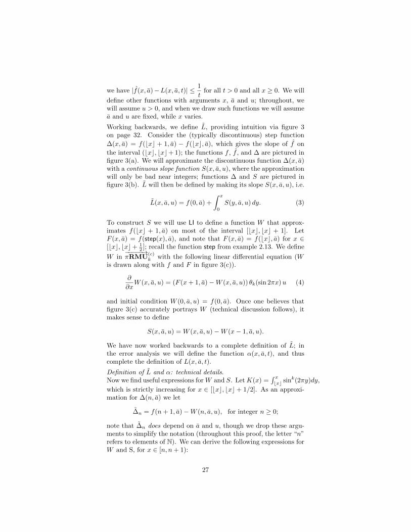
Working backwards, we define L, providing intuition via figure 3on page 32. Consider the (typically discontinuous) step function

∆(x, a) = f(bxc + 1, a) − f(bxc, a), which gives the slope of f on

the interval (bxc, bxc+ 1); the functions f , f , and ∆ are pictured infigure 3(a). We will approximate the discontinuous function ∆(x, a)with a continuous slope function S(x, a, u), where the approximationwill only be bad near integers; functions ∆ and S are pictured infigure 3(b). L will then be defined by making its slope S(x, a, u), i.e.

L(x, a, u) = f(0, a) +

∫ x

0

S(y, a, u) dy. (3)

To construct S we will use LI to define a function W that approx-imates f(bxc + 1, a) on most of the interval [bxc, bxc + 1]. LetF (x, a) = f(step(x), a), and note that F (x, a) = f(bxc, a) for x ∈[bxc, bxc+ 1

2 ]; recall the function step from example 2.13. We define

W in−−−−−→πRMU

(c)k with the following linear differential equation (W

is drawn along with f and F in figure 3(c)).

∂

∂xW (x, a, u) = (F (x+ 1, a)−W (x, a, u)) θk(sin 2πx)u (4)

and initial condition W (0, a, u) = f(0, a). Once one believes thatfigure 3(c) accurately portrays W (technical discussion follows), itmakes sense to define

S(x, a, u) = W (x, a, u)−W (x− 1, a, u).

We have now worked backwards to a complete definition of L; inthe error analysis we will define the function α(x, a, t), and thuscomplete the definition of L(x, a, t).

Definition of L and α: technical details.Now we find useful expressions forW and S. LetK(x) =

∫ xbxc sink(2πy)dy,

which is strictly increasing for x ∈ [bxc, bxc + 1/2]. As an approxi-mation for ∆(n, a) we let

∆n = f(n+ 1, a)−W (n, a, u), for integer n ≥ 0;

note that ∆n does depend on a and u, though we drop these argu-ments to simplify the notation (throughout this proof, the letter “n”refers to elements of N). We can derive the following expressions forW and S, for x ∈ [n, n+ 1):

27

W (x, a, u) = f(n+ 1, a)− ∆n Θ(x, u) (5)

S(x, a, u) = f(n+ 1, a)− f(n, a) + (∆n−1 − ∆n) Θ(x, u) (6)

where

Θ(u) = exp{−uK( 12 )}, and

Θ(x, u) =

{exp{−uK(x)}, for n ≤ x ≤ n+ 1

2 ;Θ(u), for n+ 1

2 < x < n+ 1.

The expression for S follows immediately from the expression for W ,so we now discuss the expression for W . For x ≥ 0, either ∆n = 0and W (x, a, u) = f(n + 1, a) for x ∈ [n, n + 1

2 ], or ∆n 6= 0 andthe differential equation (4) can be explicitly solved by separatingvariables. In either case, its solution for x ∈ [n, n+ 1/2] is the aboveexpression. For x ∈ [n+ 1

2 , n+ 1], ∂∂xW = 0 and thus W (x, a, u) =

W (n+ 12 , a, u).

Now we carry out the error analysis. By definition of L, the (signed)

error of approximation of f(x, a) by L is

E(x, a, u) = L(x, a, u)− f(x, a) =

∫ x

0

S(y, a, u)−∆(y, a) dy. (7)

If we let ε(u) =

∫ 12

0

exp {−uK(x)} dx+ 12 exp{−uK( 1

2 )},

∫ n+1

n

S(x, a, u)−∆(x, a) dx = (∆n−1 − ∆n) ε(u),

and the total approximation error at x = n is (using a telescopingsum):

E(n, a, u) =∑n−1i=0

∫ i+1

iS(x, a, u)−∆(x, a) dx

= (∆−1 − ∆n−1) ε(u) = −∆n−1 ε(u).(8)

For non-integer x ∈ (n, n + 1), (6) shows that S(x, a, u) is alwaysabove or below ∆(x, a), therefore E(x, a, u) is between E(n, a, u) andE(n+ 1, a, u), and so

|E(x, a, u)| ≤ max{|E(bxc, a, u)|, |E(bxc+1, a, u)|} = max{|∆bxc−1|, |∆bxc|} ε(u).

To proceed, we need to find a norm-increasing bound on ∆n thatis not dependent on u. Recall that ∆n = f(n + 1, a) −W (n, a, u).

28

By assumption f (and therefore F ) has a norm-increasing bound in−−−−−→πRMU

(c)k , so we only need to consider W . Note that W (bxc, a, u)

is in between the largest and smallest of the following three val-ues: F (bxc − 1, a), F (bxc, a) and F (bxc + 1, a); this follows fromequation 4, as illustrated in figure 3(c). Therefore, F (bxc, a) is be-tween F (x, a) and F (x − 1

2 , a) for all x. All those bounds only in-volve the function F and can be assumed norm-increasing. Theycan be combined with the bound on f to find some function β

in−−−−−→πRMU

(c)k such that max{|∆bxc−1|, |∆bxc|} ≤ β(x, a). Hence,

|E(x, a, u)| ≤ β(x, a) ε(u).

Finally, we check how ε(u) decreases with u and we use this to define

α(x, a, t) in−−−−−→πRMU

(c)k (recall that α is the missing function we use

to define L from L) such that

|E(x, a, α(x, a, t))| ≤ β(x, a) ε(α(x, a, t)) ≤ 1

t.

To do this, we need to bound ε(u). There is some κ that dependson k such that K(x) ≥ (x − bxc)κ for bxc ≤ x ≤ bxc + 1

2 . Thus, if0 ≤ x ≤ 1

2 we bound the first term of ε(u) as follows:∫ 12

0

exp {−uK(x)} dx ≤∫ 1

2

0

exp {−uxκ} dx

≤ u−1/κ

∫ +∞

0

exp{−xk}dx

≤ u−1/κ(1 +

∫ +∞

1

exp {−x} dx)

≤ 2u−1/κ.

The second term of ε(u) is 12 exp{−uK( 1

2 )} and is bounded by u−1κ

for u large enough. Therefore, β(x, a) ε(α(x, a, t)) ≤ 3β(x, a) (α(x, a, t))−1κ .

Thus, choosing a large enough α(x, a, t) ≥ (3 t β(x, a))κ we obtainthe desired 1

t bound, on |E(x, a, α(x, a, t))|.Definition of L.To conclude this part of the proof we address the case of x < 0. Wedenote by L−(x, a, t) the function that is defined from f(−x, a) in-stead of f(x, a) as in the construction above; e.g. L−(1, a, t) gives anapproximate value of f(−1, a). Notice that L(0, a, t) = L−(0, a, t) =

f(0, a) for any t. To obtain an approximation for f over R we justhave to define an appropriate convex combination of L and L−. Wewill define

L(x, a, t) = (1− λ(x, a, t))L−(−x, a, 3t) + λ(x, a, t)L(x, a, 3t), (9)

for a function λ (defined below) which resembles the Heaviside func-tion θ, but continuously and quickly switches from 0 to 1 on the

29

interval [0, δ], for a function δ = δ(a, t) which will be discussed.Therefore, L will be precisely L, for x ≥ δ, and L−, for x ≤ 0; hencethe previous error analysis still holds off of [0, δ]. Next, we consider

the error |f(x, a)− L(x, a, t)| on [0, δ].

First, we will want a function B in−−−−−→πRMU

(c)k such that |∆(x, a)| ≤

B(x, a). From the constructions above it is clear that u can bechosen large enough (depending on F and k) so that S(n, a, u)−1 ≤∆(n, a) ≤ S(n, a, u)+1 (see Figure 3(b)). Given that S is monotonicon [n, n+ 1

2 ] and constant on [n+ 12 , n+ 1], ∆(x, a) can be bounded

as follows:

min{S(x, a, u), S(x+1

2, a, u)}−1 ≤ ∆(x, a) ≤ max{S(x, a, u), S(x+

1

2, a, u)}+1,

and thus we can find such a B. To conclude part 1 of the proof weonly need B(0, a); however, we will need B(x, a) in part 2 of the

proof. Let δ(a, t) =1

B(0, a)(3t+ 1), and define

λ(x, a, t) =

{0, x ≤ 0;1, x ≥ δ(a, t), (10)

and for 0 ≤ x ≤ δ(a, t), λ(x, a, t) is increasing in x (but we donot care about its exact definition). Note that such a function λ

is in−−−−−→πRMU

(c)k (even though we do not have the exact division

operation needed for δ, we can define a non-zero decreasing functionthat converges to zero faster than 1/x, such as e−x). The error,

|f(x, a) − L(x, a, t)|, for x ≤ 0 or x ≥ δ(a, t) has been done, sowe consider the case of 0 < x < δ(a, t) (some technical discussionfollows to justify the second equality):

|f(x, a)− L(x, a, t)| = |f(x, a)− {(1− λ(x, a, t))L−(−x, a, 3t) + λ(x, a, t)L(x, a, 3t)}|= |f(x, a)− (1− λ(x, a, t))f(0, a)− λ(x, a, t)L(x, a, 3t)|≤ |f(x, a)− f(0, a)|+ λ(x, a, t)|L(x, a, 3t)− f(0, a)|≤ |f(x, a)− f(0, a)|+ λ(x, a, t){|L(x, a, 3t)− f(x, a)|+ |f(x, a)− f(0, a)|}≤ ∆(0, a)δ(a, t) + 1 · (|L(x, a, 3t)− f(x, a)|+ ∆(0, a)δ(a, t))

≤ 1

3t+

1

3t+

1

3t

≤ 1

t

To justify the second equality we point out why L−(−x, a, 3t) =f(0, a), for 0 < x < δ(a, t). Assume that δ(a, t) ≤ 1

2 , which isguaranteed if B(0, a) ≥ 2. We make the following claim:

For any f , any u and x ∈ [− 12 , 0], L(x, a, u) = f(0, a).

30

We apply this to f(−x, a) and u = 3t to conclude that L−(x, a, 3t) =f(0, a), and thus L−(−x, a, 3t) = f(0, a) for x ∈ [0, 1

2 ]. To prove the

claim, it suffices (by the definition of L) to show that S(x, a, u) = 0for x ∈ [− 1

2 , 0], and thus (by definition of S) it suffices to show thatW (x, a, u) = f(0, a) for x ∈ [− 3

2 , 0]. To prove the last point, we recall

that W (0, a, u) = f(0, a) and show that ∂∂xW = 0 for x ∈ [− 3

2 , 0].To get the derivative to be zero, we consider the definition of Win equation (4), and it suffices to note that: For x ∈ [− 3

2 ,−1] orx ∈ [− 1

2 , 0], θk(sin 2πx) = 0 and for x ∈ [−1,− 12 ], by definition,

F (x+ 1, a) = f(0, a).

Part 2.

For |x− x′| ≤ 1 we have

|f(x, a)− f(x′, a)| ≤ |x− x′| max{|∆(x, a)|, |∆(x′, a)|},

since ∆ gives the slope of f . In part 1, we saw that there is a function

B in−−−−−→πRMU

(c)k such that |∆(x, a)| ≤ B(x, a). We use it to bound

max{|∆(x, a)|, |∆(x′, a)|} by some M(x, a) in−−−−−→πRMU

(c)k ; then we

can simply take m(x, a, z) = M(x, a)z.

�

The basic point of the next corollary is that from an approximation to afunction, we can construct an approximation to its full linearization, and geta genuine modulus for the linearization. Basically, repeated application of thelast lemma yields the corollary.

Corollary 4.10. If f(x) � f∗(x, t) and f∗ is in−−−−−→πRMU

(c)k , then there are

functions L and m in−−−−−→πRMU

(c)k such that Lin(f) � L and m is a modulus for

Lin(f).

Proof

Suppose f(x1, . . . , xn) � f∗(x1, . . . , xn, t), where f∗ is in−−−−−→πRMU

(c)k .

Let f0 = f , and let fk+1 = Lin(fk, xk+1).

We proceed by induction on k from 0 up to n, showing:

There are Lk and norm-increasing mk in−−−−−→πRMU

(c)k such

that for x1, . . . , xk ∈ R, and xk+1, . . . , xn ∈ Z:

1. |fk(x1, . . . , xn)− Lk(x1, . . . , xn, t)| ≤1

t, and

2. |x1−x′1|+ . . .+ |xk−x′k| ≤1

mk(x1, . . . , xn, z)implies

|fk(x1, . . . , xn)− fk(x′1, . . . , x′k, xk+1, . . . , xn)| ≤ 1

z.

31

1.0 1.5 2.0 2.5 3.0 3.5 4.0 4.5 5.0

−4

−3

−2

−1

01

23

4

(a)

1.0 1.5 2.0 2.5 3.0 3.5 4.0 4.5 5.0

−4

−3

−2

−1

01

23

4

1.0 1.5 2.0 2.5 3.0 3.5 4.0 4.5 5.0

−4

−3

−2

−1

01

23

4

●

●

●

● ●

f

f ..

1.0 1.5 2.0 2.5 3.0 3.5 4.0 4.5 5.0

−4

−3

−2

−1

01

23

4

(b)

1.0 1.5 2.0 2.5 3.0 3.5 4.0 4.5 5.0

−4

−3

−2

−1

01

23

4

(b)

●

●

●

● ●

S

1.0 1.5 2.0 2.5 3.0 3.5 4.0 4.5 5.0

−1

01

23

4

(c)

1.0 1.5 2.0 2.5 3.0 3.5 4.0 4.5 5.0

−1

01

23

4

1.0 1.5 2.0 2.5 3.0 3.5 4.0 4.5 5.0

−1

01

23

4

W

F

f

Figure 3: Constructions in lemma 4.9 for fixed a and u:(a) The dotted line represents f(x) and the thin solid line represents f(x) = Lin(f, x), which

we aim to approximate; the slope of f(x) is given by ∆(x), which is represented by the thick,discontinuous solid line.(b) We approximate ∆(x) by S(x, u), represented by the continuous line, where S(x, u) =W (x, u)−W (x− 1, u).(c) This figure illustrates the construction of W from f : The dotted line represents f(x) asbefore, the thin solid line represents F (x), which is constant on the intervals [n, n+ 1/2], andthe thick solid line represents W (x, u) as defined from F with the linear differential equation(4); the figure shows that W (x, u) is close to F (n), and thus to f(n), for most of x ∈ [n−1, n].Note that the graph of W was in fact obtained by numerically integrating (4) with u = 10.

32

When k = n, we have proved the corollary. For k = 0, we takeL0 = f∗, and we need no m0 (we may take it to be identicallyzero so the inductive step works). We now complete the proof bydiscussing the inductive step from k to k + 1. Inductively, we haveappropriate Lk and mk. Let Lk = Lin(Lk, xk+1) and note that fromthe inductive hypothesis and the definition of Lin, we have:

(�) For x1, . . . , xk+1 ∈ R, xk+2, . . . , xn ∈ Z, |fk+1(x1, . . . , xn)−Lk(x1, . . . , xn, t)| ≤ 1/t.

From lemma 4.9 we have L and m in−−−−−→πRMU

(c)k such that:

• Lk � L

• |xk+1 − x′k+1| ≤1

m(x1, . . . , xn, t, z)implies

|Lk(x1, . . . , xn, t)− Lk(x1, . . . , xk, x′k+1, xk+2, . . . , xn, t)| ≤

1

z

Let Lk+1(x1, . . . , xn, t) = L(x1, . . . , xn, 2t, 2t). For x1, . . . , xk+1 ∈R, and xk+2, . . . , xn ∈ Z: |fk+1(x1, . . . , xn) − Lk(x1, . . . , xn, 2t)| ≤1

2tby �, and |Lk(x1, . . . , xn, 2t) − Lk+1(x1, . . . , xn, t)| ≤

1

2tby the

definition of L, thus by the triangle inequality, Lk+1 appropriatelyapproximates fk+1.

Now we consider the modulus claim. By definition,−−−−−→πRMU

(c)k con-

tains a norm-increasing bound on |m|; we use the same name “m”

for this bound. Let b be some norm-increasing function in−−−−−→πRMU

(c)k

such that |x|+ 1 ≤ b(x). Let mk+1(x1, . . . , xn, z) =

1+mk(x1, . . . , xk, b(xk+1), xk+2, . . . , xn, 5z)+m(b(x1), . . . , b(xk), xk+1, . . . , xn, 5z, 5z).

It is a norm-increasing function in−−−−−→πRMU

(c)k . Now we check the

main property for modulus functions. Suppose we have some

x1, . . . , xk+1, x′1, . . . , x

′k+1 ∈ R, xk+2, . . . , xn ∈ Z satisfying:

|x1 − x′1|+ . . .+ |xk+1 − x′k+1| ≤1

mk+1(x1, . . . , xn, z).

Consider:

(F) |fk+1(x1, . . . , xn)− fk+1(x′1, . . . , x′k, xk+1, . . . , xn)|.

Letting r = bxk+1c, by definition of Lin, (F) equals:

|(r+1−xk+1)(fk(x1, . . . , xk, r, xk+2, . . . , xn)−fk(x′1, . . . , x′k, r, xk+2, . . . , xn))

+(xk+1−r)(fk(x1, . . . , xk, r+1, xk+2, . . . , xn)−fk(x′1, . . . , x′k, r+

1, xk+2, . . . , xn))|.

33

Since |r|, |r + 1| ≤ b(xk+1) and

mk+1(x1, . . . , xn, z) ≥ mk(x1, . . . xk, b(xk+1), xk+2, . . . , xn, 5z), weuse the inductive hypothesis and the fact that mk is norm-increasing,

to bound (F) by2

5z. Now consider

|fk+1(x1, . . . , xn)− fk+1(x′1, . . . , x′k+1, xk+2, . . . , xn)| ≤

|fk+1(x1, . . . , xn)− fk+1(x′1, . . . , x′k, xk+1, . . . , xn)|

+ |fk+1(x′1, . . . , x′k, xk+1, . . . , xn)−Lk(x′1, . . . , x

′k, xk+1, . . . , xn, 5z)|

+ |Lk(x′1, . . . , x′k, xk+1, . . . , xn, 5z)−Lk(x′1, . . . , x

′k, x′k+1, xk+2, . . . , xn, 5z)|

+ |Lk(x′1, . . . , x′k, x′k+1, xk+2, . . . , xn, 5z)−fk+1(x′1, . . . , x

′k, x′k+1, xk+2, . . . , xn)|.

In the above sum of four terms, the first is bounded by2

5z, since

it is (F); we observe that the other three terms are each bounded

by1

5z, thus providing the desired

1

zbound. The second and fourth

terms are bounded by1

5zbecause of �. For the third term, we note

that |x′i| ≤ b(xi) since mk+1(x1, . . . , xn, z) ≥ 1, thus using the factthat m is norm-increasing we get:

m(x′1, . . . , x′k, xk+1, . . . , xn, 5z, 5z) ≤ m(b(x1), . . . , b(xk), xk+1, . . . , xn, 5z, 5z)

= mk+1(x1, . . . , xn, z)

By the properties of m we bound the third term by1

5z.

�

The next lemma shows that if a function has the right shape for the MUoperation (definition 3.12) over the naturals, then the approximate linearizationhas the analogous behavior over the reals.

Lemma 4.11. Suppose f(y, z) is in−−−−−→πRMU

(c)k , and f|Z(y, z) satisfies: a) the

conditions of MU when y, z ≥ 0, b) f|Z(y, z) = 0 when y < 0, and c) f|Z(y, z) =f|Z(y, 0) when z < 0.

Then there is a function L(y, z, t) in−−−−−→πRMU

(c)k such that:

1. Lin(f) � L,

2. For any z and t, L(y, z, t) increases with y,

3. For any z and t, there is exactly one y∗ such that L(y∗, z, t) = 1, and forthis unique y∗, ∂

∂yL(y∗, z, t) > 0,

4. For any y and t, L(y, z, t) decreases with z.

Proof

34

The basic approach of the proof is to use the proof of lemma 4.9,first with respect to y (i.e. y plays the role of x), applied to thefunction f(y, z), to arrive at the function L1(y, z, t1). Then we usethe proof of lemma 4.9 again, but now with respect to z (i.e. z playsthe role of x), and applied to the function L1(y, z, t1), to arriveat the function L2(y, z, t1, t2), so that our desired function will beL(y, z, t) = L2(y, z, 2t, 2t).

When we use the proof of lemma 4.9 to get L1 we write L1 in placeof L, and W1 in place of W ; likewise we write L2 in place of L, andW2 in place of W , when getting L2. By assumption, for a integer z,there is a natural yz such that f(yz, z) = 1; note that yz = y0 fornegative integer z.

Parts 1, 2 and 3. Recall that in lemma 4.9, the constructionworked by first constructing the function L(y, z, u), then lettingL(y, z, t) = L(y, z, α(y, z, t)), for a certain function α that dependson y, z, and t. In this proof, we make a key modification at thispoint (both for L1 and L2), choosing an α which depends only ont. Recall that we chose α(y, z, t) such that β(y, z)ε(α(y, z, t)) ≤ 1/t.In the current situation, due to the particular shape of f , we canbound β(y, z) by 3 (independent of y, z): Recall that β was definedon page 29 to be a bound on max{|∆n−1|, |∆n|}, approximations tothe slope of f (with respect to y or z), which for the exact slopewould be at most 2, and for sufficiently large u is less than 3 (sincewe substitute α(t) for u, we just assume that we have taken α(t) tobe sufficiently large). Thus in the construction of L1, based on f ,and L2, based on L1 (where L1 inherits the rough shape of f), wecan take α to be a function just of t. The same argument appliesto the definition of λ and δ in (10) to conclude we can take δ as afunction of just t, λ (in the construction of L1) as a function of justy and t, and λ (in L2) as a function of just z and t.

Construction for L1.

We begin by considering L1, showing that for z restricted to beingan integer, ∂

∂yL1(y, z, t1) ≥ 0, and for y > yz − 1, ∂∂yL1(y, z, t1) > 0

(note that since L1 approximates f , the positive derivative afteryz − 1 is enough to guarantee that L1 has a unique one, at whichit has a positive derivative, i.e. part 3 of the lemma). Since L1 isdefined as in (9), we will first prove the claim for L1 on y ≥ 0; theargument extends to L−1 on y ≤ 0. Finally, we will consider theinterval [0, δ], where L1 is a combination of L1 and L−1 .

Since L1(y, z, t1) = L1(y, z, α(t1)), we analyze L1(y, z, u). We rewrite(6) to get

∂

∂yL1(y, z, u) = [f(n+1, z)−f(n, z)] (1−Θ(y, u))+[W1(n, z, u)−W1(n−1, z, u)] Θ(y, u),

(11)

35

for y ∈ [n, n+1). Note that 0 < Θ(u) ≤ Θ(y, u) ≤ 1; hence the aboveexpression is a convex combination of f(n+ 1, z)− f(n, z), which isnon-negative by hypothesis, and W1(n, z, u)−W1(n−1, z, u), whichwe claim is also non-negative. To show this, consider integer k ≥ 0and y ∈ [k, k + 1), letting y → k + 1 in (5) to derive the followingrecurrence:

W1(k + 1, z, u) = [1−Θ(u)] f(k + 1, z) + Θ(u)W1(k, z, u). (12)

This is now a convex combination of f(k + 1, z) and W1(k, z, u).

We now proceed by induction on k, up to n, showingW1(k+1, z, u) ≥W1(k, z, u). For k = 0, this is true, since W1(0, z, u) = f(0, z), andwe can use (12) to conclude that W1(1, z, u) ≥ f(0, z) = W1(0, z, u).Furthermore, if W1(k, z, u) ≥W1(k−1, z, u) then by (12) and the as-sumption that f(k+1, z) ≥ f(k, z) we conclude thatW1(k+1, z, u) ≥[1 − Θ(u)] f(k, z) + Θ(u)W1(k − 1, z, u) = W1(k, z, u). Therefore,W1(n, z, u) ≥W1(n− 1, z, u), so the difference W1(n, z, u)−W1(n−1, z, u) ≥ 0, as desired. Thus ∂

∂y L1(y, z, u) ≥ 0 for all y ≥ 0.

To show ∂∂y L1 > 0 for y > yz − 1, we consider two cases: yz −

1 < y < yz and y ≥ yz. We use equation (11) in both cases,showing that either its first term or its second term is positive (wejust showed that both terms of (11) are non-negative). In the caseyz − 1 < y < yz, Θ(y, u) < 1, and f(yz, z)− f(yz − 1, z) = 1, so thefirst term is positive. In the case y ≥ yz, Θ(y, u) > 0 (it always is)and by induction on integer n ≥ yz, W1(n, z, u) > W1(n−1, z, u), sothe second term is positive (the induction is similar to the previousinduction, again using (12)).

To conclude, we consider L1 over R. Recalling (9), for y ≥ δ(t1), L1

is L1, and for y ≤ 0, L1(y, z, t1) = L−1 (−y, z, t1); the former case wasjust analyzed, and the latter case can be handled similarly (in fact,the shape of f makes L−1 (−y, z, t1) = 0 for all y ≤ 0). We just needto show that L1(y, z, t1) is also increasing for 0 ≤ y ≤ δ(t1). Withoutloss of generality we suppose that δ(t) ≤ 1

2 , so the expression of L1

simplifies to

L1(y, z, t1) = (1− λ(y, t1))f(0, z) + λ(y, t1)L1(y, z, 3t1), (13)

as seen at the end of part 1 of lemma 4.9. Since f(0, z) = L1(0, z, 3t1)and L1(y, z, 3t1) is increasing in y, L1 is increasing on [0, δ].

Construction for L2.

Now we consider L2(y, z, t1, t2), the construction of lemma 4.9 ap-plied to L1, linearizing with respect to z; so now z plays the role ofx, and a is y together with t1. Let L1 = Lin(L1, z); the construction

we are now carrying out will approximate L1. We show that theearlier properties of L1 that held for integer z, also hold for all real

36

z; in particular, for all z, ∂∂yL2 ≥ 0, and there is some yz such that

the one of L2 occurs after yz − 1 and ∂∂yL2 > 0 for y > yz − 1.

We start by considering the function L2(y, z, t1, t2), for z ≥ 0; atthe end we briefly discuss L2. Consider z ∈ [n, n + 1) for someinteger n ≥ 0, and focus on L2(y, z, t1, u), where L2(y, z, t1, t2) =L2(y, z, t1, α(t2)). We derive from (7) and (8) two convenient ex-pressions when z ∈ [n, n+ 1):

L2(y, z, t1, u) = L1(y, z, t1)− [ε(u)− σ(z, u)] ∆n−1 − σ(z, u) ∆n

= A1(z, u) L1(y, n, t1) +A2(z, u) L1(y, n+ 1, t1)++ [ε(u)− σ(z, u)]W2(y, n− 1, t1, u) + σ(z, u)W2(y, n, t1, u)

(14)where σ(z, u) =

∫ zn

Θ(r, u)dr, A1(z, u) = n+ 1− z − ε(u) + σ(z, u),and A2(z, u) = z − n− σ(z, u).

Now we differentiate (14) with respect to y to write

∂∂y L2(y, z, t1, u) = A1(z, u) ∂

∂yL1(y, n, t1) +A2(z, u) ∂∂yL1(y, n+ 1, t1)+

+ [ε(u)− σ(z, u)] ∂∂yW2(y, n− 1, t1, u) + σ(z, u) ∂

∂yW2(y, n, t1, u).

(15)Is is easy to check the following facts (for z ∈ [n, n + 1]): σ(z, u)is strictly increasing; σ(n, u) = 0; σ(n + 1, u) = ε(u); z − n ≥σ(z, u); and n + 1 − z ≥ ε(u) − σ(z, u). Hence A1, A2, ε(u) −σ(z, u), σ(z, u) ≥ 0 for z ∈ [n, n+1]. We have shown that ∂

∂yL1(y, n+

1, t1), ∂∂yL1(y, n, t1) ≥ 0, so to prove that L2 has the desired proper-

ties, it suffices to show that for integer k = 0, . . . , n, ∂∂yW2(y, k, t1, u) ≥

0 and furthermore, if y > yk−1 then ∂∂yW2(y, k, t1, u) > 0. We prove

these facts by induction on k up to n, similar to the inductive proofsused in the construction of L1. The induction proceeds like before,using the following recurrence (which can be derived from equation(12)):

∂

∂yW2(y, k, t1, u) = [1−Θ(u)]

∂

∂yL1(y, k, t1)+Θ(u)

∂

∂yW2(y, k−1, t1, u).

Recalling once again (9), for z ≥ δ(t2), L2(y, z, t1, t2) = L2(y, z, t1, t2),and for z ≤ 0, L2(y, z, t1, t2) = L−2 (y,−z, t1, t2). Using the same ar-guments as above, it is clear that L2(y, z, t1, t2), satisfies ∂

∂yL2 ≥ 0

and ∂∂yL2 > 0 for y > yz − 1. To show that this property holds for

L2 when 0 < z < δ(t2), as before we write

L2(y, z, t1, t2) = [1−λ(z, t2)] L1(y, 0, t1)+λ(z, t2)L2(y, δ(t2), t1, 3t2).

Differentiating with respect to y yields the result, since λ does notdepend on y, and both ∂

∂yL1 and ∂∂yL2 have the right properties.

37

In the end we take L(y, z, t) = L2(y, z, 2t, 2t), which has the desiredproperties.

Part 4. Analogous to (11), for z ∈ [n, n+ 1),

∂

∂zL2(y, z, t1, u) = [L1(y, n+ 1, t1)− L1(y, n, t1)] (1−Θ(z, u))+

[W2(y, n, t1, u)−W2(y, n− 1, t1, u)] Θ(z, u),(16)

which we now claim is less than or equal to 0. The argument issimilar to the one after (11), except that this time the relevant termsin (16) are non-positive. First, L1(y, n + 1, t1) − L1(y, n, t1) ≤ 0because of the shape of f (recall figure 1), i.e. since for all n ∈ N,L1(y, n+ 1, t1) is just L1(y, n, t1) shifted to the right (or not shiftedat all) in the y direction. To prove that W2(y, n, t1, u) −W2(y, n −1, t1, u) ≤ 0 we use the fact that L1(y, n + 1, t1) − L1(y, n, t1) ≤ 0and we proceed inductively along the same lines of the argumentthat follows (12). Note that for integer n < 0, the constructionreveals that W2(y, n, t, u) = W2(y, n − 1, t, u) so the difference is 0.Finally, we adjust the argument surrounding (13) to L2, to concludethat L2 is decreasing with respect to z ∈ R (in equation (12), andthe discussion following it, W2 is used in place of W1 and L1 in placeof f).

�

Remark In the last lemma, we can replace the single parameter z by a tuple,since we can repeat the construction of L2 of lemma 4.11 for each member ofthe tuple (similar to corollary 4.10).

Now we prove the final and most important approximation of figure 2, mak-ing significant use of the last corollary and lemma. Proceeding in a straight-forward way we ran into difficulties, and thus we generalize the inductive hy-pothesis, so that we simultaneously build approximating functions and modulusfunctions.

Lemma 4.12. QMU(1) � πRMU(1)k for any k ≥ 1.

Proof

Since−−−−−→πRMU

(1)k ⊆ πRMU

(1)k , it suffices to show QMU(1) �

−−−−−→πRMU

(1)k .

We proceed inductively on the construction of the function algebraQMU(c), showing the following stronger claim (for both c = 0 andc = 1):

For any f(x) in QMU(c) the following two properties hold,

1. (Approximation property) There is f∗(x, t) in−−−−−→πRMU

(c)k such

that f � f∗, and

38

2. (Modulus property) There is m(x, z) in−−−−−→πRMU

(c)k which is a

modulus for f .

We will use a few functions in the proof which are similar to thefunction step (recall example 2.13), and can be defined using it,

or defined in a similar manner, all in−−−−−→πRMU

(0)k . We can define

a continuous integer rounding function rd : R → R which has thefollowing property: For any n ∈ N, rd(x) = n for all x ∈ [n −1/4, n+ 1/4], and for x ≤ 0, rd(x) = 0. We can define a continuoussign function sg : R → R such that sg(x) = 0 for x ≤ 0, andsg(x) = 1 for x ≥ 1; its values for 0 < x < 1 do not matter.

Now we discuss the steps of the induction, showing the approxima-tion and modulus property in each case; technically we also proceedinductively on the rank c, though in our case we just do it for c = 0and then for c = 1.

• Basic Functions.

The modulus of all the basic functions are simple to deal with,so we just consider the approximation property. Except for

θ1 and div,−−−−−→πRMU

(0)k contains expansions to R of the basic

functions of QMU(c), and so approximates them exactly. For

θ1 and div, we find functions in−−−−−→πRMU

(0)k which approximate

these functions on Z, and then we linearize to approximatethe functions everywhere. For θ1, for x ∈ Z, θ1(x) = rd(x),an exact approximation on Z, and thus by corollary 4.10 wecan approximate θ1 on all of Q. For div, we use the function

E(x, t) =

1− e−tx

x, if x 6= 0;

t, if x = 0., a function in

−−−−−→πRMU

(0)k

such that for x ∈ [1,+∞), we have |1/x−E(x, t)| ≤ 1/t (E wasdefined by Bournez and Hainry [5], directly before proposition11). Let f(x, t) = E(x, t) · sg(x) + sg(−x+ 1), so div|Z � f , andthus by corollary 4.10 we can approximate div on all of Q.

• Composition.

Consider f(g(x)) in QMU(c) (for composition with more func-tions, the argument is similar), where inductively we have f∗(y, t1), g∗(x, t2)

in−−−−−→πRMU

(c)k such that f � f∗ and g � g∗, andmf (y, z),mg(x, z)

in−−−−−→πRMU

(c)k , which are modulus functions for f and g, respec-

tively. Note that g(x) ≤ g∗(x, 1) + 1, and since the latter func-

tion is in−−−−−→πRMU

(c)k we can find a function b in πRMU

(c)k such

that |g(x)| ≤ b(x) and b is norm-increasing. Thus, mg(x,mf (b(x), z))

is in−−−−−→πRMU

(c)k and it is a modulus for f ◦ g. For the approxi-

mation we note that:

f(g(x)) � f∗(g∗(x,mf (b(x), 2t)), 2t),

39

where the latter function is in−−−−−→πRMU

(c)k .

• Sums and Products.

We will use the following claim (follows from [9, lemma 4.7]):

If F (x, a) is in−−−−−→πRMU

(c)k and takes natural values on

natural inputs, then there is a G(y, a) in−−−−−→πRMU

(c)k

such that for y, a ∈ N, G(y, a) =

y∑x=0

F (x, a); the claim

also holds for products replacing sums.

Consider f(x, a) in QMU(c) and let g(y, a) be∑

Q applied tof and the argument x; note that since

∑Q can be applied, f

must be natural valued on natural inputs. Inductively we have

some f∗(x, a, t) in−−−−−→πRMU

(c)k such that f � f∗; thus F (x, a) =

rd(f∗(x, a, 4)) is in−−−−−→πRMU

(c)k . Notice that f(x, a) = F (x, a)

for x, a ∈ N. We apply the above claim to obtain some G(y, a)

in−−−−−→πRMU

(c)k such that g(y, a) = G(y, a), for y, a ∈ N. Using

the function sg from above we can ensure that G(y, a) = 0 forinteger arguments y, a when at least one argument is negative;thus g(y, a) = G(y, a) for all y, a ∈ Z. By definition 3.22,

∑Q

returns a linearization, therefore g = Lin(g). Thus

corollary 4.10 applied to G gives us an approximation functionand modulus function for g. The argument for

∏Q is basically

the same.

• Linearization (Lin). This step follows immediately from corol-lary 4.10.

• Search Operation (MUQ).

For simplicity, we only consider a function of two variables (see

the remark following lemma 4.11). Consider f(y, z) in QMU(0)

satisfying the requirements of MUQ, and we let g(z) = MUQ(f),

so g is in QMU(1). It will be useful to recall the example afterdefinition 3.22.

We let yz ∈ N denote the unique one of f for z ∈ N, i.e. thevalue yz such that f(yz, z) = 1 (recall that by definition 3.22,for z ∈ N, we have yz ∈ N). Thus f(y, z) = 0 for naturaly ≤ yz − 1, f(yz, z) = 1, and f(y, z) = 2 for natural y ≥yz + 1 (note that yz ≥ 1 by definition 3.12 so f(0, z) = 0).

Inductively, we have some f∗(y, z, t) in−−−−−→πRMU

(0)k such that f �

f∗. As we did in the case of sums and products, we consider thefunction rd(f∗(y, z, 4)), which is exactly equal to f(y, z) overthe naturals. Using that function together with sg, we obtain afunction F (y, z) such that for natural y, z, F (y, z) = f(y, z), fornegative integers z, F (y, z) = f(y, 0), and for negative integersy, F (y, z) = 0.

40

Since we have no control over how f (and thus F ) behavesoff of the integers, we apply lemma 4.11 to F (y, z) to ob-tain L(y, z, t), an approximation of Lin(f). By conditions 2and 3, the requirements of UMU are met, thus we can de-fine G(z, t) = UMU(L(y, z, t) − 1, y) which finds the root ofL(y, z, t) − 1, with respect to y. Since Lin(f) � L (by condi-tion 1 of lemma 4.11), yz, the one of f (with respect to y) iswithin 1

t of the zero of L(y, z, t) − 1. This key point is guar-anteed since the slope of Lin(f) with respect to y is 1 near yz;if the slope near yz were very small, the zero of L(y, z, t) − 1could be far from yz. By condition 4, G is norm-increasing and

so in−−−−−→πRMU

(1)k . By definition 3.22, MUQ returns a lineariza-

tion, therefore g = Lin(g); thus corollary 4.10 supplies us with

a modulus in−−−−−→πRMU

(1)k .

�

5. Conclusion

A major advance of the three characterizations of theorem 2.17 is that theyuse notions from analysis instead of notions from classic computability. In termsof the proof techniques, the advance is in the use of our method of approxima-tion. At the end of the conclusion we present an open question that we hopecan be solved using the method of approximation.

The characterizations of CR in the style of Ko [23], which have some similar-ity to our work, in fact rely heavily on classic computability. We can view ourtheorem 2.17 as exhibiting a dense subset of CR, together with an appropriateway to “complete” the class. For example, given a function f(x) in CR, by ourtheorem we must have a function f∗(x, t) in ODE?

k such that f = limt→∞

f∗. If

we just consider t ∈ N, we can view f∗(x, t) as a sequence of functions con-verging uniformly to f . Ko also characterizes CR by exhibiting functions whichconverge uniformly to the functions of CR (see [23, theorem 2.15]). However inKo’s characterization, the uniform convergence is controlled by requiring thatthe convergence proceed computably; thus Ko’s approach (and similarly envi-sioned modifications) use classical notions of computability in the characteriza-tion itself. In our approach we avoid the drawback of using computability in ourdefinition of limits or elsewhere, thus ODE?

k(LIM) provides a more genuinelydistinct characterization of CR.

To highlight the significance of the proof technique of approximation, wecompare our proof to the approach of Bournez and Hainry [6]. Most of thework, for us and them (though, they show something slightly different) goesinto showing the main lemma 3.6, CR ⊆ RMUk(LIM). Starting with a functionf in CR, they proceed directly to an approximation F (x, t) in RMUk, withoutpassing through intermediary classes as we do (the notion of approximation isnot stated explicitly in their work). Like us, they, apply LIM with respect to the

41

argument t to obtain the result. Deviating from us, they use the fact that thereis an elementary computable map which takes a modulus for f and a pair ofintegers (at, bt) which code an approximation of x, and returns a pair of integers(pt, qt) which code an approximation of f(x) (t is the approximation parameter).They show how that integer map can be embedded in RMUk, and they showhow to regularize (similar to linearizing) the embedding to build F (x, t) inRMUk, a uniform approximation for all x in the compact domain of f . Themodulus of f is a crucial ingredient in the construction. Since the techniquesapplied in [6] do not exhibit a modulus for f (see [6, Remark 7.1]) they rely onthe fact that C2 functions on compact intervals have a (non constructive) trivialuniform modulus, which they use in the construction of F . Instead, we carrythe modulus throughout our proof. Using the notion of one class of functions

approximating another class of functions, we are able to show CR � πRMU(1)k ,

with no additional restrictions, which implies the desired inclusion.Since our approximation notion is transitive, we have broken up this approx-

imation into a series of approximations, using some well-chosen intermediaryclasses of functions. The technique also allows us to work with function alge-bras rather than notions from classical computability (i.e. we avoid extensivework with the Turing machine definition of computable analysis). With func-tion algebras, it is convenient to work with their inductive structure, a prooftechnique which works well with the method of approximation. The methodappears amenable to generalization. As evidence of this, we see that in ourproof, of the four approximations (recall figure 2), three are virtually the sameas ones proved in our earlier paper [12]. In the context of a more general theoryof approximation (future work), a number of approximations should follow fromgeneral facts, concentrating the work on the approximations that are importantfor the problem at hand. Thus we see this work as another step towards a moregeneral theory that could have broad application to other problems of this sort.

We now discuss a possible improvement of our result. In our paper [10], wewere able to remove the function θk from the basic functions, while maintain-ing the characterization of the elementary computable functions. This is nicebecause it makes the characterization even more simple, and furthermore theunderlying function algebra (before the limit operation is applied) is then a col-lection of analytic functions. In our earlier work [10], we were able to dispensewith the function θk, using our method of approximation, essentially showingthat it suffices to work with an approximation of θk that can be built with otherfunctions in the function algebra. This approach has difficulties in the contextof this paper, and so we are led to the following interesting question (supposingFk is one of the real function algebras we have considered in this paper, let Fbe the same function algebra, but without the basic function θk):

Question Does CR = RMU(LIM) = INV(LIM) = ODE?(LIM)?

The last characterization by ODE?(LIM) would be especially interesting,since ODE? is essentially the widely studied class of real primitive recursivefunctions.

42

6. Acknowledgements

This work was partially supported by Fundacao para a Ciencia e a Tec-nologia and EU FEDER POCTI/POCI, and grant SFRH / BPD / 16936 /2004.

References

[1] L. Blum, F. Cucker, M. Shub, and S. Smale. Complexity and Real Compu-tation. Springer-Verlag, New York, NY, 1998.

[2] L. Blum, M. Shub, and S. Smale. On a theory of computation and complex-ity over the real numbers: NP-completeness, recursive functions and univer-sal machines. Bulletin of the American Mathematical Society, 21(1):1–46,July 1989.

[3] O. Bournez and M. L. Campagnolo. A survey on continuous time computa-tions. In S.B. Cooper, B. Lowe, and A. Sorbi, editors, New ComputationalParadigms. Changing Conceptions of What is Computable, pages 383–423.Springer-Verlag, New York, 2008.

[4] O. Bournez, M. L. Campagnolo, D. S. Graca, and E. Hainry. Polynomialdifferential equations compute all real computable functions on computablecompact intervals. Journal of Complexity, 23(3):317–335, 2007.

[5] O. Bournez and E. Hainry. Elementarily computable functions over thereal numbers and R-sub-recursive functions. Theoretical Computer Science,348(2–3):130–147, 2005.

[6] O. Bournez and E. Hainry. Recursive analysis characterized as a class ofreal recursive functions. Fundamenta Informaticae, 74(4):409–433, 2006.

[7] V. Brattka. Recursive characterization of computable real-valued functionsand relations. Theoretical Computer Science, 162(1):45–77, 1996.

[8] V. Brattka and P. Hertling. Feasible real random access machines. Journalof Complexity, 14(4):490–526, 1998.

[9] M. L Campagnolo, C. Moore, and J. F. Costa. An analog characterizationof the Grzegorczyk hierarchy. Journal of Complexity, 18:977–1000, 2002.

[10] M. L. Campagnolo and K. Ojakian. Using approximation to relate com-putational classes over the reals. In J. Durand-Lose and M. Margenstern,editors, MCU 2007, volume 4664 of Lecture Notes in Computer Science,pages 39–61. Springer-Verlag, 2007.

[11] M. L. Campagnolo and K. Ojakian. Characterizing computable analy-sis with differential equations. In V. Brattka, R. Dillhage, T. Grubba,and A. Klutsch, editors, Fifth International Conference on Computabilityand Complexity in Analysis, volume 221 of Electronic Notes in TheoreticalComputer Science, pages 23–35, 2008.

43

[12] M. L. Campagnolo and K. Ojakian. The elementary computable functionsover the real numbers: applying two new techniques. Archive for Mathe-matical Logic, 46(7-8):593–627, 2008.

[13] P. Collins and D. S. Graca. Effective computability of solutions of ordi-nary differential equations - the thousand monkeys approach. In ElectronicNotes in Theoretical Computer Science – Proceedings of the Fifth Inter-national Conference on Computability and Complexity in Analysis (CCA2008), volume 221, pages 103–114, 2008.

[14] P. Collins and D. S. Graca. Effective computability of solutions of differen-tial inclusions — the ten thousand monkeys approach. Journal of UniversalComputer Science, 15(6):1162–1185, 2009.

[15] J.F. Costa, B. Loff, and J. Mycka. A foundation for real recursive functiontheory. Annals of Pure and Applied Logic, 160(3):255 – 288, 2009.

[16] N. Cutland. Computability: An introduction to recursive function theory.Cambridge University Press, 1980.

[17] A. Edalat and P. Sunderhauf. A domain-theoretic approach to computabil-ity on the real line. Theoretical Compututer Science, 210(1):73–98, 1999.

[18] D. S. Graca and J. F. Costa. Analog computers and recursive functionsover the reals. Journal of Complexity, 19(5):644–664, 2003.

[19] D. S. Graca, N. Zhong, and J. Buescu. Computability, noncomputabil-ity and undecidability of maximal intervals of IVPs. Transactions of theAmerican Mathematical Society, 361(6):2913–2927, 2009.

[20] A. Grzegorczyk. Computable functionals. Fund. Math., 42:168–202, 1955.

[21] P. Hartman. Ordinary Differential Equations. Birkhauser, 2nd edition,1982.

[22] A. Kawamura. Differential recursion. ACM Transactions on ComputationalLogic, 10(3), 2009.

[23] K.-I. Ko. Complexity Theory of Real Functions. Birkhauser, 1991.

[24] W. Maass. Networks of spiking neurons: the third generation of neuralnetwork models. Neural Networks, 10:1659–1671, 1997.

[25] C. Moore. Recursion theory on the reals and continuous-time computation.Theoretical Computer Science, 162:23–44, 1996.

[26] M. B. Pour-El and J. I. Richards. Computability in analysis and physics.Perspectives in mathematical logic. Springer-Verlag, 1989.

[27] F.P. Preparata and M.I. Shamos. Computational geometry: an introduc-tion. Springer-Verlag New York, Inc., New York, NY, USA, 1985.

44

[28] C. Shannon. Mathematical theory of the differential analyzer. Journal ofMathematical Physics, 20:337–354, 1941.

[29] K. Weihrauch. Computable Analysis: An Introduction. Springer-Verlag,2000.

45

Index

Classes of functionsINVk, 8

INV(c)k , 8

πRMU(c)k , 7

RMUk, 7

RMU(c)k , 7

QMU(c), 18

˜dQMU(1)

, 19dQMU(c), 19NMU, 15NMU(c), 15ODEk, 8ODE?

k, 8−−−−−→πRMU

(c)k , 25

L, 11CN, 14dCQ, 16CR, 4CQ, 15QMU, 18

dCQ, 19BH, 11FA, 4G, 11

Functionssg, 39rd, 39θ, 7θk, 7D, 16. , 15b·c, 17div, 18sign, 16step, 8|·|, 17N, 16d·c, 22d·e, 17

OperationsMUQ, 18

∑Q, 18

µ, 14MU, 14LIM, 10∏

, 14∑, 14

UMU, 6LI, 5Lin, 17comp, 5Inverse, 6ODE, 5

PropertiesD−free, 19Nice, 13Norm-increasing, 17well-posed, 5

Approximation, 13�, see approximation

Linearization, 17

Modulus, 17

Rank, 7

Transitivity, 14

46