This is the author manuscript accepted for publication and has undergone full peer review but has not been through the copyediting, typesetting, pagination and proofreading process, which may lead to differences between this version and the Version of Record . Please cite this article as doi: 10.1111/caje.12263 This article is protected by copyright. All rights reserved Author Manuscript

Welcome message from author
This document is posted to help you gain knowledge. Please leave a comment to let me know what you think about it! Share it to your friends and learn new things together.
Transcript

This is the author manuscript accepted for publication and has undergone full peer review but has
not been through the copyediting, typesetting, pagination and proofreading process, which may
lead to differences between this version and the Version of Record. Please cite this article as doi:
10.1111/caje.12263
This article is protected by copyright. All rights reserved
Auth
or
Manuscript

International trade and unionization: evidence
from India
Reshad N. Ahsan University of Melbourne
Arghya Ghosh University of New South Wales
Devashish Mitra Syracuse University
Abstract. We exploit exogenous variation in tariffs to examine the impact of import competition on union-
ization and union wages in a developing country. Using a combination of nationally representative house-
hold data (National Sample Survey Organization) and nationally representative industry-level data (Annual
Survey of Industries) from India, we find that net-import industries that experienced larger cuts in tariffs
also experienced larger declines in unionization. In addition, we find that these industries also experienced
larger increases in union wages. These results are consistent with the predictions of an efficient bargaining
framework that we extend to endogenize the union formation decision by allowing for a fixed cost of union
formation. We also conduct a back-of-the-envelope calculation to show that the total wage gains to union-
ized workers marginally exceed the total wage losses to deunionized workers.
JEL Classification: F16, J50, O53
Corresponding author: Devashish Mitra, [email protected]
We thank the editor, John Ries, and an anonymous referee for helpful comments and suggestions. We also thank
seminar and conference participants at Brandeis University, Louisiana State University, Southern Methodist Uni-
versity, the University of Oregon, the Asian Meeting of the Econometric Society (AMES), and the Econometric
Society Australasian Meetings (ESAM) for useful comments. The standard disclaimer applies.
Thisarticleisprotectedbycopyright.Allrightsreserved
Auth
or
Manuscript

1 Introduction
Due to a dramatic expansion of international trade, the past few decades have been heralded as
a new wave of globalization.1 A distinguishing feature of this new wave is the unprecedented
participation of developing countries. For example, during the period 1993 to 2004, the total
exports of goods and services from low-income countries grew at an annual rate of 8.27% while the
growth rate for the rest of the world was 6.94%.2 Similarly, Goldberg and Pavcnik (2007) identify a
long list of developing countries that undertook significant trade reforms during this period. While
this unprecedented participation in international trade has undoubtedly brought many benefits, it
has also raised concerns about the income of low-skilled workers in these countries.
One of the channels through which trade can lower the income of low-skilled workers is by
lowering union density as well as union wages. There are two main ways in which this can occur.
First, trade can lower union density and wages by decreasing the rents available for bargaining
between the firm and the union. Second, as Rodrik (1997) has pointed out, trade can also lower
the bargaining power of workers by making them more replaceable.3 Both of these factors will
undermine the bargaining power of unions and thereby diminish a union’s ability to compress
dispersion in wages. This is a particularly important issue for developing countries as they tend
to have relatively lower union density to begin with (Freeman 2009). Despite this, very little is
known about how international trade affects unionization or union wages in a developing country.
We address this gap in the literature by examining the impact of import tariff liberalization
(tariff liberalization from hereon) on unionization and union wages in India. India provides an ideal
setting in which to examine this question for two reasons. First, faced with an acute fiscal crisis in
1991, the newly elected government in India enacted dramatic trade reforms at the urging of the
International Monetary Fund (IMF). By our estimates, tariffs fell from an average of 147.2% in
1988 to 106.1% in 1992 and 23.8% in 2003. Thus, while there was a large drop in average tariffs
by 1992, there continued to be significant cuts in tariffs thereafter. Importantly, given that the
decision to lower tariffs was done under external pressure, the post-1991 changes provide us with
exogenous variation in tariffs that can be exploited to examine its causal effects on unionization
and union wages. Second, this was also a period of rapid changes in unionization and union wages
in India. Our data suggest that the percentage of individuals that are members of a union fell from
28.3% in 1993 to 21.9% in 2004. Similarly, we observe a seven-fold increase in average daily
union wages between 1993 and 2004. Surprisingly, we observe that the increase in union wages
was relatively higher in net-import industries.
To what extent are these changes in unionization and union wages related to tariff liberaliza-
1World Bank (2002) distinguishes between three waves of globalization: the first wave (1870 to 1914), the second
wave (1945 to 1980), and the new wave (1980 onwards).2The growth rates are based on our calculations using data from the World Development Indicators (WDI). We
chose 1993 because it is the earliest year for which the WDI reports the total exports of goods and services for low-
income countries. We use the WDI’s own classification to categorize countries as low income.3In particular, the import of final goods can make the products produced by domestic workers more substitutable.
In turn, this will lead to domestic workers becoming more substitutable. In addition, the import of intermediate inputs
can directly make domestic workers more substitutable.
2
Thisarticleisprotectedbycopyright.Allrightsreserved
Auth
or
Manuscript

tion? We use two sources of data to explore these relationships further. First, we use nationally
representative household surveys spanning the period 1993 to 2004 to construct measures of union-
ization. These data are from the National Sample Survey Organization (NSSO). These surveys ask
respondents whether there was any union in their activity and whether they were a member of
a union. As these surveys are repeated cross-sections, we aggregate the responses to create an
industry-state-year panel. We then use these data to examine the impact of lower industry tariffs
on unionization. Our results suggest that a decrease in industry tariffs led to a decrease in unioniza-
tion and union membership in net-import industries. This effect was smaller in states with flexible
labor markets. In addition, we also use our data to calculate the average daily union wage at the
industry-state-year level. Using these data, we find that a decline in tariffs led to an increase in
union wages in net-import industries.
To rationalize these results, we extend the efficient bargaining framework used in McDonald
and Solow (1981) and Brock and Dobbelaere (2006) by allowing for a fixed cost of union formation
that enables us to endogenize the union formation decision. Using this model we show that the
deunionization caused by tariff liberalization can be explained by a reduction in rents that such
liberalization brings about. The decreased rents acts as a disincentive against the maintenance
and formation of unions as well as their membership. We expect this effect to be stronger in net-
import industries where the reduction in rents are likely to be disproportionately greater. In our
model, we also show that by lowering the price that domestic import-competing firms can charge,
tariff liberalization also lowers the employment and output of domestic firms. With diminishing
marginal product of labor and the presence of some fixed factors of production, it follows that the
average and marginal product of labor will increase as a result of tariff liberalization. In turn, the
real union wage (measured in units of the industry’s final output) will also increase as a result of
tariff liberalization in net-import industries. In addition to explaining our empirical results, our
model highlights the underlying mechanisms driving these results. Using industry-level Annual
Survey of Industries data spanning the period 1993 to 2004 we find empirical support for these
proposed mechanisms.
Our results suggest that the impact of tariff liberalization on union wages is not uniform across
all unionized workers. On the one hand, we find that a fraction of the initially unionized workers
transition into nonunion employment due to tariff liberalization. As a result, these workers earn the
lower nonunion wage. On the other hand, we find that workers that remained unionized after tariff
liberalization experienced an increase in their wages. To gauge the net effect, we conduct a back-
of-the-envelope calculation to compare the wage losses to deunionized workers with the wage
gains to unionized workers. Our calculations indicate that the total gains to unionized workers
marginally exceed the total losses to deunionized workers. Thus, it suggests that even if tariff
liberalization causes deunionization in net-import industries, it need not decrease the total wage
income of the pool of initially unionized workers in these industries.
Our paper is related to an extensive literature on trade and unionization, with the empirical
side focused primarily on developed countries. On the theoretical side, Grossman (1984) examines
the impact of trade on union membership and wages, while Mezzetti and Dinopoulos (1991) and
Bastos and Kreickemeier (2009) examine the impact of trade on union wage bargaining and there-
3
Thisarticleisprotectedbycopyright.Allrightsreserved
Auth
or
Manuscript
fore on union wages. In addition, Gaston and Trefler (1995), Bastos, Kreickemeier and Wright
(2010) examine, both theoretically and empirically, the impact of trade/product market compe-
tition on union wages using U.S. and U.K. data respectively. Interestingly, Gaston and Trefler
(1995) find that lower tariffs in the U.S. are associated with higher union wages. However, they
also find that other measures of trade (i.e. imports and exports) do not support this conclusion. In
addition, Bastos, Kreickemeier and Wright (2010) find that, for low levels of unionization, greater
product market competition increases union wages in the U.K. However, this effect is reversed for
unionization levels above a certain threshold.
A key contribution to the empirical literature on the impact of trade on unionization is the
monograph by Baldwin (2003). He finds that trade had a modest effect, if any, on union patterns
and the union-nonunion wage differential in the U.S. Similarly, Magnani and Prentice (2003) also
find that increased imports did not have an effect on unionization. Dreher and Gaston (2007) find
that social integration (“spread of ideas, information, images and people” leading to the “Ameri-
canization of institutions”) rather than economic integration has led to deunionization in the OECD
countries in their sample. Thus, empirical studies in the trade and unionization literature either fo-
cus on how trade affects unionization or how trade affects wages in a unionized setting. In fact,
the literature has mainly focused on the latter issue with the former being relatively under-studied.
Further, the main focus of this literature has been on developed countries.4 In contrast, our empir-
ical study of trade and unionization in India (a large developing country) examines the impact of
trade on both unionization and union wages.
The remainder of this paper is structured as follows. In section 2 we discuss the institutional
background of collective bargaining in India as well as our main hypotheses. In section 3 we
discuss the data used to construct our measures of unionization and union wages. Next, in sec-
tion 4 we describe our econometric method. In section 5 we discuss our results. In section 6 we
discuss a model that rationalizes our empirical results and allows us to investigate the underlying
mechanisms driving our results. Finally, in section 7 we provide a conclusion.
2 Background and Main Hypotheses
2.1 Unions in India
Article 19(c) of the Indian Constitution guarantees the right to association to all citizens of India.
Further, the Trade Union Act 1926 allows any seven workers within a firm to form a union (Bhag-
wati and Panagariya 2013). The relative ease of registering unions in India has meant that they are
quite common at the firm or plant level. Venkata Ratnam and Verma (2011), while acknowledg-
ing the difficulty of obtaining accurate figures, believe that the number of unions in India exceeds
100,000. This is likely to be an underestimate given that there are unregistered or unofficial unions
that are not included in these official statistics. As discussed below, an advantage of our data is
that it reports the union status of workers in both registered and unregistered unions. As a result,
4The only developing country study on this issue we are aware of is Shendy (2010), who finds that trade liberal-
ization in South Africa lowered wages in industries with high levels of unionization.
4
Thisarticleisprotectedbycopyright.Allrightsreserved
Auth
or
Manuscript
our data represent a more representative sample of unionized workers.5
According to Venkata Ratnam (2009), collective bargaining in India takes place at different
levels depending on the industry. In industries where government enterprises are dominant, such as
banking, coal, steel etc., bargaining typically takes place at the national level. In contrast, bargain-
ing takes place at the industry-region level in some of the private-sector dominated industries such
as cotton, jute, textiles, engineering, and tea. However, even in these industries, the industry-region
level agreements are only binding for employers that have authorized their regional employer as-
sociations in writing to negotiate on their behalf. Otherwise, collective bargaining takes place at
the firm level. In the rest of the private sector, bargaining takes place at the firm level or some-
times even at the plant level. This is especially the case in more recent years where most collective
bargaining takes place at a fairly decentralized level (Hiers and Kuruvilla 2000).
Since independence, excessive state involvement in industrial relations has meant that most
key Indian unions have been closely aligned with major political parties. It is widely believed that
such alignments have weakened unions and have prevented them from responding dynamically
to changing economic conditions (Hill 2009). Partly in response to the poor performance of these
centralized and unrepresentative unions, there has been a proliferation of independent or politically
unaffiliated unions since the late 1970s. These unions, which were not guided by political concerns,
were able to negotiate higher wages and fringe benefit packages for its workers (Bhattacharjee
1999) and have become increasingly common in India. Thus, to summarize, private-sector unions
in India are increasingly politically unaffiliated and increasingly negotiate directly with firms. Our
model in section 6.1 will capture these features of the private-sector industrial relations system in
India.
One final aspect of industrial relations that matters in our context is how Indian unions treat
non-members. The most prevalent system in India is a union shop where an employee of a firm
must become a member of a union associated with that firm after being hired (Venkata Ratnam and
Verma 2011). It is important to note that the union shop setup is in between a closed shop and an
open shop. In the closed-shop case, only union members can be hired by a firm. In contrast, in the
open-shop case, union membership is not a condition for being hired or for continued employment.
Our model in section 6.1 has a closed-shop union although we also survey some open-shop models.
However, this is not a very consequential assumption. Indeed, if we extend our model to a union-
shop system, our results will not change.6
5Registered unions in India are most active in the public sector and among relatively large firms, and are relatively
less prevalent in the informal sector. However, our data are based on answers to survey questions and include both
formal and informal sector workers, thereby also allowing us to observe the union status of the latter (who, if unionized,
are mostly likely to be members of unregistered unions).6For example, we could have political entrepreneurs or union leaders penetrating firms and opening unions without
any membership to begin with. The wage and employment could then be determined through union-firm bargaining.
Such a union would care about the welfare of its expected membership, which will figure in its objective function
during the bargaining process. Once employed by a unionized firm, employees will have to join the union. With such
a change in our framework, all our results will remain unchanged.
5
Thisarticleisprotectedbycopyright.Allrightsreserved
Auth
or
Manuscript

2.2 Hypotheses About Tariff Liberalization, Unionization, and Wages
The Indian trade reforms of 1991 mainly consisted of reductions in tariff and non-tariff barriers to
imports. Thus, this liberalization led to greater import competition. Such competition is expected
to lead to the destruction of monopoly power of domestic import-competing firms and the rents
that come with such power. Alternatively, even in the presence of perfect competition, lower
barriers to imports will reduce the rents earned by fixed and specific factors. These rents (as well
as any reductions or increases in them) are often shared with unions and, therefore, with unionized
workers. As these rents go down with import competition, one would expect that the net rents
extracted by a union (net of the costs of running the union) will also decrease. It follows that
unions that are sufficiently costly to run will drop out as a result of the tariff reductions. Moreover,
fewer workers will want to join unions since their benefits from such membership over and above
their union dues will shrink. Thus, both the number of unions and union membership will decrease
as a result of tariff reductions. Since comparative disadvantage industries (or net-import industries)
will experience the greatest reduction in prices as a result of tariff liberalization, we expect these
industries to suffer relatively larger, adverse effects on unionization and union membership.7 These
effects are summarized by the following hypothesis:
HYPOTHESIS 1. Greater import competition through tariff liberalization will lead
to deunionization. That is, a smaller proportion of workers employed in an industry
facing greater import competition will be unionized. This is especially the case in
net-import industries.
By lowering the price that domestic import-competing firms can charge, tariff liberalization
is also expected to lower the employment and output of domestic firms. With constant returns to
scale technology and the presence of some fixed factors, the lower employment will increase the
average and marginal product of labor. In turn, this will increase the real wage rates (measured in
units of the industry’s final output) of both unionized and nonunionized labor.8 Thus, we have the
following second hypothesis.
HYPOTHESIS 2. Greater import competition through tariff liberalization will lead to
an increase in the real union wage (measured in units of the firm’s actual output).
7In practice, in almost every industry there are both imports and exports (i.e. there is intra-industry trade), and a
reduction in the tariff on imports directly competing with the domestic output of an industry (whether a net-export
or net-import industry) will result in a decline in the domestic price charged by firms in that industry. However, the
relative importance of tariff reductions is expected to be higher in net-import industries and, therefore, the domestic
price decline from a given reduction in its own tariff is also expected to be greater.8Under perfect competition, the real wage rate of a nonunionized worker will equal her marginal product. In the
case of a unionized worker, one part of her real wage will be due to her marginal product, while the other part will
be her share of the rents extracted by her union. Note that in real terms (in terms of units of the final output of the
firm), the rent per worker will be the output per worker minus the outside or alternative real wage. In our theoretical
framework, which is presented later in this paper, we show that this alternative wage is equal to the marginal product
of labor. This result comes from the first-order conditions associated with the Nash bargaining problem between the
firm and the union. Thus, the union wage rate will be a function of the marginal and average product of labor and will
be increasing in both.
6
Thisarticleisprotectedbycopyright.Allrightsreserved
Auth
or
Manuscript
3 Data
The unionization measures used in our empirical work were constructed using data from the
“employment-unemployment” household surveys conducted by India’s National Sample Survey
Organisation (NSSO). We use three rounds of these nationally-representative surveys: round 50
(1993–1994), round 55 (1999–2000), and round 61 (2004–2005).9 Unfortunately data on union-
ization were not collected in previous rounds. As a result, we are unable to examine unionization
patterns using these data for the pre-1993 period.
The “employment-unemployment” household surveys collect demographic and employment
information on all household members. Apart from standard employment information, these sur-
veys also ask respondents about unions in their activity. In particular, individuals were asked
whether there was any union/association in their activity (union presence). In addition, individuals
were asked, conditional on there being a union/association in their activity, whether they were a
member (union membership). As these surveys are repeated cross-sections, we aggregated indi-
vidual responses to both questions to the 3-digit industry and state level.10 The union presence
aggregate captures the fraction of individuals in a given industry and state that work in unionized
activities. Similarly, the union membership aggregate captures the fraction of individuals in a given
industry and state that are members of a union. When calculating these aggregates, we weighted
each observation using an individual’s sample weight. In addition, we restricted the sample to
individuals that were in the labor force, worked in manufacturing industries, and were between the
ages of 14 and 65. We also restricted the sample to the fifteen major states in India. Both measures
of unionization vary by 3-digit industry, state, and year. The correlation coefficient between them
is 0.88.
Table 1 lists the trends in unionization by year and various individual characteristics. Panel
A lists the trends in the union presence data. The second column suggests that union presence
declined by 19% from 34.9% in 1993 to 28.2% in 2004. This percentage decline was lower for
workers with at least a secondary education (high-skilled) as compared to workers without a sec-
ondary education (low-skilled). In addition, columns (5) to (8) suggest that the percentage decline
in union presence was also greater for younger and female workers. Panel B lists the trends in
the union membership data. Overall, union membership declined by 22.6% from 28.3% in 1993
to 21.9% in 2004. Once again we observe that the percentage decline in union membership was
relatively greater for low-skilled, younger, and female workers.
The “employment-unemployment” household surveys also collected wage data for both union-
ized and nonunionized workers. These wages represent each respondent’s earnings during the week
prior to the survey date. A limitation of the wage data is that it was not consistently defined across
the three survey rounds. In particular, in rounds 50 (1993) and 61 (2004), the NSSO’s definition
of wages excluded ‘overtime’ payments for additional work done beyond normal working hours.
9In the remainder of this paper, we refer to each of the three survey years using the first year of the survey. In other
words, we refer to 1993–1994 as 1993.10Throughout this paper, industries are classified according to the 1987 National Industrial Classification (NIC).
There are 104 such industries in our sample.
7
Thisarticleisprotectedbycopyright.Allrightsreserved
Auth
or
Manuscript

050
10
015
020
0A
vera
ge
Daily
Un
ion W
ag
e (
Rs.)
1993 2004
Net Importer Net Exporter
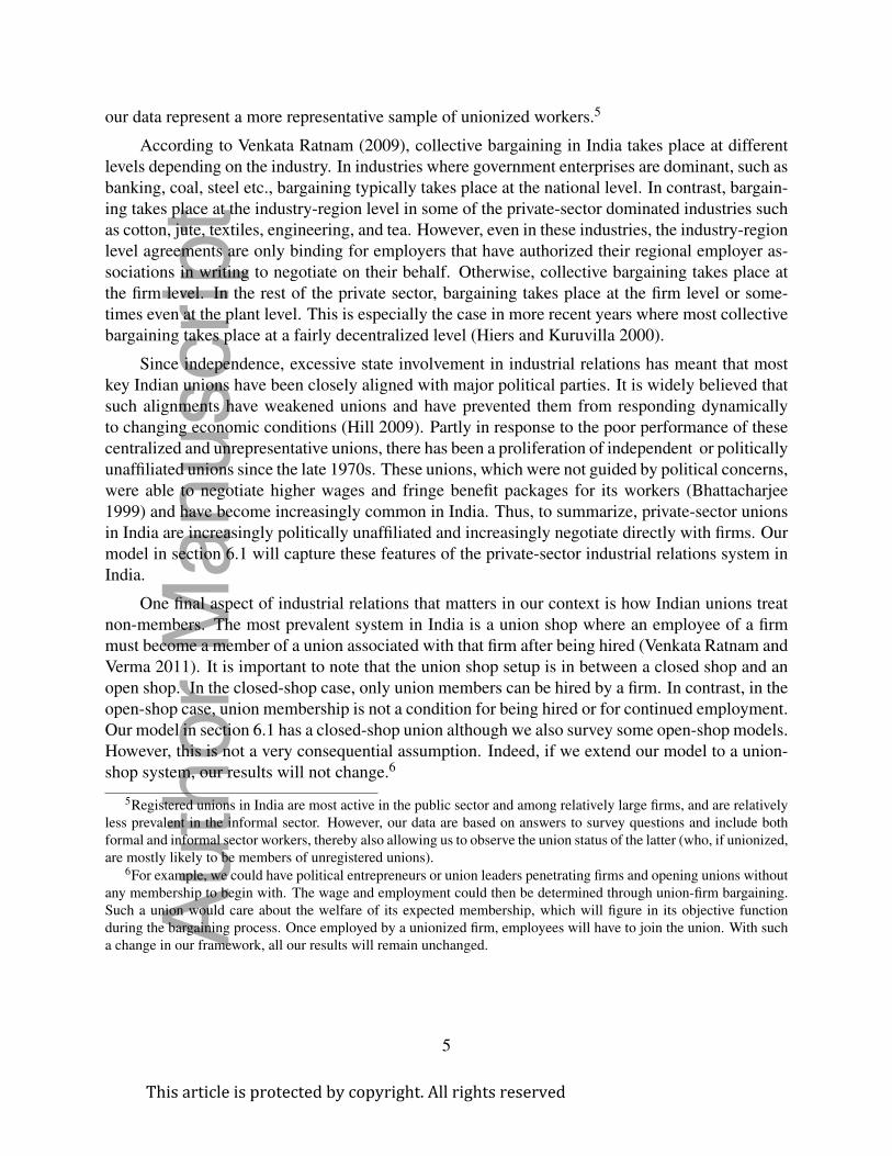
Figure 1: Trends in average daily union wage by industry type. The wage data are from the
National Sample Survey Organization’s (NSSO) “employment-unemployment” surveys.
However, in round 55 (1999), the wage data included these ‘overtime’ payments. Given that there
was no information provided on ‘overtime’ hours worked, we were unable to adjust the round 55
wage data to make it comparable to the other rounds. Instead, we omitted round 55 from our
NSSO-based wage analysis.11
Next, we construct our net import indicator using data from the NBER-United Nations Trade
Data (Feenstra, Lipsey, Deng, Ma and Mo 2005). This dataset provides bilateral trade flows be-
tween countries at the 4-digit Standard International Trade Classification (SITC) revision 2 level.
We converted India’s trade data to the 3-digit National Industrial Classification (NIC) 1987 level.12
After this conversion, we have access to the total imports and exports for each 3-digit Indian in-
dustry in our sample.
Figure 1 depicts the trends in average daily union wages for both net-import and net-export
industries. To the extent that tariff liberalization disproportionately lowers union rents in net-
import industries, we would expect union wages in these industries to grow at a slower rate. The
trends in Figure 1 indicate that the opposite is true. Average daily union wages in net-import
industries have increased at a faster rate relative to union wages in net exporter industries.
11We use all three rounds of data for our unionization analysis.12This conversion involved several steps. First, we used a crosswalk available at Marc-Andreas Muendler’s webpage
to convert the SITC classification to International Standard Trade Classification (ISIC), revision 2. We then used a
crosswalk made available by the United Nations Statistics Division to convert the data from ISIC revision 2 to ISIC
revision 3. The latter is identical to the Indian NIC 1998 classification. Lastly, we used our own crosswalk to convert
the data from ISIC, revision 3/NIC 1998 to NIC 1987.
8
Thisarticleisprotectedbycopyright.Allrightsreserved
Auth
or
Manuscript
050
010
00
15
00
20
00
Ou
tput p
er
Wo
rker
(Rs. T
hou
san
ds)
1990 1995 2000 2005Year
Net Importer Net Exporter
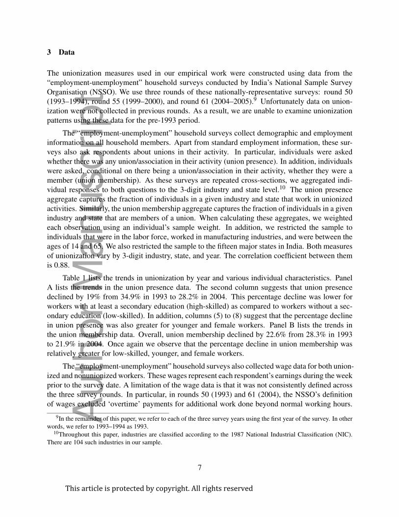
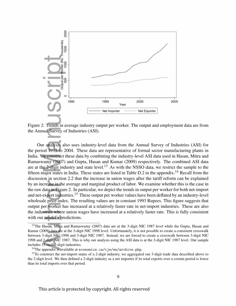
Figure 2: Trends in average industry output per worker. The output and employment data are from
the Annual Survey of Industries (ASI).
Our analysis also uses industry-level data from the Annual Survey of Industries (ASI) for
the period 1993 to 2004. These data are representative of formal sector manufacturing plants in
India. We construct these data by combining the industry-level ASI data used in Hasan, Mitra and
Ramaswamy (2007) and Gupta, Hasan and Kumar (2009) respectively. The combined ASI data
are at the 2-digit industry and state level.13 As with the NSSO data, we restrict the sample to the
fifteen major states in India. These states are listed in Table D.2 in the appendix.14 Recall from the
discussion in section 2.2 that the increase in union wages after the tariff reform can be explained
by an increase in the average and marginal product of labor. We examine whether this is the case in
the raw data in Figure 2. In particular, we depict the trends in output per worker for both net-import
and net-export industries.15 These output per worker values have been deflated by an industry-level
wholesale price index. The resulting values are in constant 1993 Rupees. This figure suggests that
output per worker has increased at a relatively faster rate in net-import industries. These are also
the industries where union wages have increased at a relatively faster rate. This is fully consistent
with our model’s predictions.
13The Hasan, Mitra and Ramaswamy (2007) data are at the 3-digit NIC 1987 level while the Gupta, Hasan and
Kumar (2009) data are at the 3-digit NIC 1998 level. Unfortunately, it is not possible to create a consistent crosswalk
between 3-digit NIC 1998 and 3-digit NIC 1987. Instead, we are forced to create a crosswalk between 3-digit NIC
1998 and 2-digit NIC 1987. This is why our analysis using the ASI data is at the 2-digit NIC 1987 level. Our sample
includes 15 such 2-digit industries.14The appendix is available at economics.ca/cje/en/archive.php.15To construct the net-import status of a 2-digit industry, we aggregated our 3-digit trade data described above to
the 2-digit level. We then defined a 2-digit industry as a net importer if its total exports over a certain period is lower
than its total imports over that period.
9
Thisarticleisprotectedbycopyright.Allrightsreserved
Auth
or
Manuscript
Next, the data on output tariffs are from the Asian Development Bank (ADB) and are an
extension of the series used by Hasan, Mitra and Ramaswamy (2007). These data cover the period
between 1988 and 2003. The original data are at the sector level and were converted to 1987
National Industrial Classification (NIC) industries.16,17 These data suggest that tariffs fell from
an average of 147.2% in 1988 to 106.1% in 1992 and 23.8% in 2003. Thus, while there was an
immediate drop in average tariffs after 1991, there continued to be significant cuts in tariffs during
our sample period of 1992 to 2003.18 Note that these tariffs vary by industry and year, but not by
state. Summary statistics for all variables reported in the regression tables are listed in Table 2. All
monetary values reported in this paper are in constant 1993 Rupees.19
4 Econometric Method
4.1 Trade and Unionization
Our hypotheses in section 2.2 were that (a) tariff liberalization will lead to deunionization and (b)
that tariff liberalization will increase real union wages. In addition, we argued that these effects will
be stronger for net-import industries. We now describe the econometric strategy we use to test these
predictions. First, we examine the relationship between tariff liberalization and deunionization
using the following econometric specification:
Uist = αu +β1Tari f fit−1 +β2NMi ×Tari f fit−1 +β3Zit−1 +β4Xist +θi +θs +θt + εist (1)
where Uist is the degree of unionization in a 3-digit industry i, state s, and year t. We use two
alternative measures of unionization. Our first measure is the fraction of individuals in a given
industry and state that work in unionized activities. We refer to this as union presence. Our second
measure is the fraction of individuals in a given industry and state that are members of a union. We
refer to this as union membership.
Tari f fit−1 is the one-year lagged import tariff in 3-digit industry i. To test whether the impact
of tariffs depends on the trade orientation of an industry, we add an interaction between Tari f fit−1
and NMi. The latter is a time-invariant dummy variable that is one for industries with positive
net imports.20 The inclusion of NMi into this specification raises endogeneity concerns if it is the
case that the trade orientation of an industry is correlated with factors that also affect the extent
of unionization and union wages in an industry. To address these concerns, we construct NMi
using pre-1993 data. The use of such lagged data minimizes the possibility of endogeneity in this
16We thank Rana Hasan at the ADB for providing us the tariff data.17These sectors do not map to all of the three-digit industries in our sample. In the event that a three-digit industry
does not have tariff data, we substitute the appropriate two-digit average tariff.18Recall that our unionization data are for the years 1993, 1999, and 2004. However, because we are using lagged
tariffs in our econometric specification (see below), the relevant time span for tariffs in our application is 1992 to 2003.191 US dollar in 1993 was approximately equal to Rs. 31.20Thus, our identification of β2 comes from (a) variation in tariffs over time, (b) cross-industry variation in tariffs
and (c) cross-industry variation in NMi.
10
Thisarticleisprotectedbycopyright.Allrightsreserved
Auth
or
Manuscript

context. To construct this indicator, we define an industry as a net importer if its average exports
over the period 1988 to 1992 was lower than its average imports during this period. We use these
five-year averages to ensure that our net-import indicator is not contaminated by transitory changes
in imports and exports in an industry.
Zit−1 includes controls for the skill intensity and the degree of competition in an industry.
Both of these are likely to affect the degree of unionization. We proxy skill intensity using the one-
year lagged ratio of non-production to production workers in an industry. We proxy the degree of
competition using the natural logarithm of one-year lagged output per plant in an industry. Both of
these industry-level measures are constructed using the ASI data. In equation (1) we also include
a vector of control variables, Xist , that includes the fraction of casual workers in total employment,
the fraction of household employees in total employment, the fraction of workers employed in rural
areas, the fraction of old (age > 40) and young (age < 30) workers in total employment, and the
fraction of educated workers (secondary education and above) in total employment. All variables
included in Xist are aggregated from the NSSO data and vary by industry, state, and year. Lastly, θi,
θs, and θt are industry, state, and year fixed effects respectively while εist is an error term. Based
on Hypothesis 1, we expect β1 and especially β1 +β2 to be positive.
4.2 Trade and Union Wages
Our second hypothesis in section 2.2 was that tariff liberalization will increase real union wages.
We explore this relationship using a two-stage approach. In the first stage, we estimate the follow-
ing econometric specification:
ln(Wh) = γ t0 + γ t
1Xh +ωh (2)
where Wh is the daily wage earned by worker h, Xh is a series of worker-level controls that includes
a worker’s age, age squared, as well as indicators for male, rural, household head, Hindu, scheduled
caste/tribe, and educational attainment, and ωh is a classical error term.21 We estimate equation
(2) separately for each round of NSSO data that we use. As a result, the coefficients γ t0 and γ t
1 are
NSSO-round specific. Further, when estimating these regressions we weight each observation with
the corresponding individual’s survey weight. The estimated residuals from (2), ωh, represent the
part of a worker’s wage that is not explained by her observable characteristics.
We aggregate these residuals to the industry-state-year level by calculating a weighted aver-
age, where the weights are each individual’s sample weights provided by the NSSO. In particular,
to generate the union wage for each industry-state-year cell, we calculate the average residual wage
21The NSSO data categorizes a respondents’ educational level into various categories. We place each respondent
into one of the following five categories: (a) not literate, (b) below primary, (c) primary, (d) middle school, (e)
secondary school, and (f) graduate and above. We then include indicators for educational attainment levels (b) to (f)
with (a) being the omitted category.
11
Thisarticleisprotectedbycopyright.Allrightsreserved
Auth
or
Manuscript

for all union workers in that cell as follows:
WUist =
nUist
∑hU
ist=1
σhUist
∑nU
ist
hUist=1
σhUist
× ωhU
ist
where i indexes industries, s indexes states, t indexes years. hUist indexes unionized workers in a
particular industry, state, and year, nUist is the total number of unionized workers in that industry-
state-year cell while σhUist
denotes the sampling weights provided by the NSSO. We use an equiv-
alent method to calculate the average nonunion wage in each industry-state-year cell. We refer to
the W ’s as adjusted union/nonunion wages from hereon. The advantage of using adjusted wages is
that it will be independent of observable compositional and demographic factors. This will not be
the case if we were to calculate average industry-state-year wages using the raw wage, Wh.22
Next, we estimate the following econometric specification in the second stage:
WUist = δ0 +δ1Tari f fit−1 +δ2NMi ×Tari f fit−1 +δ3Zit−1 +θi +θs +θt + εist (3)
where εist is an error term. All other control variables in equation (3) are as defined earlier. Note
that having controlled for demographic and other controls in the first stage, we no longer include
the vector of controls, Xist , in equation (3).
A general concern with our econometric approach is the potential endogeneity of output tar-
iffs. Endogeneity may arise if both unionization/union wages and output tariffs are correlated
with political economy factors such as industry size, lobbying power and so forth. Such concerns
are less relevant in our context due to the exogenous nature of the Indian trade reforms of 1991.
As mentioned earlier in the paper, the reforms were undertaken as a precondition for obtaining
emergency loans from the IMF. Given earlier attempts to avoid IMF loans and the associated con-
ditionalities, the adoption of these reforms came as a surprise (Hasan, Mitra and Ramaswamy
2007). Thus, not only were these reforms due to external pressure, their timing was such that In-
dian industries were likely unable to anticipate it. Thus, the post-1991 changes in tariffs associated
with these reforms are likely to be exogenous to political economy factors. In addition, all regres-
sions in this paper include industry fixed effects, which will capture the effect of any time-invariant
political economy factors.
A related concern with our econometric strategy is the presence of reverse causality. In partic-
ular, it could be the case that unions in India exerted influence over the central government’s trade
policies. This would imply that post-reform changes in tariffs in India were a function of initial
level of unionization and union wages. To examine whether this is the case, we use the following
strategy. We first aggregate our unionization and union wages measures by 3-digit industry and
year. We then regress current tariffs on one-period lagged unionization and union wages. Here
period refers to the various survey years. For example, we regress 1998 tariffs on 1993 unioniza-
22We also conduct our wage-based analysis using weighted averages of the raw wage data. As we show below, our
primary results are robust to using this alternate measure.
12
Thisarticleisprotectedbycopyright.Allrightsreserved
Auth
or
Manuscript

tion levels. These regressions include year and industry fixed effects and are weighted by the total
number of workers in an industry. The aim of these regressions is to examine whether levels of
unionization and union wages are related to subsequent changes in trade policy.
5 Results
5.1 Unionization
Table 3 lists the results from estimating equation (1). The dependent variable in columns (1) to
(3) is the fraction of workers in a given 3-digit industry, state, and year that work in unionized
activities (union presence). Note that all regressions reported in Tables 3 to 5 include 3-digit
industry, state, and year fixed effects. In addition, the standard errors are robust and clustered
at the 3-digit industry level. We begin in column (1) by estimating the average effect of tariff
liberalization on union presence. The coefficient of interest suggests that lower output tariffs, on
average, did not have a statistically significant effect on union presence. Next, we describe the
coefficient estimates of the control variables included in this regression but not reported in Table
3. The coefficient of skill intensity suggests that union presence was higher in industries with
higher ratio of non-production to production workers. On the other hand, we find that industrial
concentration did not have a statistically significant effect on union presence.23 Lastly, we also find
that union presence was lower in industry-state pairs where there were more low-skilled workers,
younger workers (age < 30), casual workers, household employees, and rural workers.
In column (2) we examine whether the impact of tariff liberalization on unionization depends
on the trade orientation of an industry. To do so, we interact an indicator for whether an industry
is a net importer with output tariffs and add it to our specification. The estimates in column (2)
suggest that lower output tariffs led to an overall decline in union presence in net-import industries.
This is indicated by the positive and significant coefficient of the interaction term that is larger
in magnitude than the negative coefficient of the tariff level term. In fact, these results suggest
that, given a 10 percentage point decline in output tariffs, union presence in net-import industries
declined by an additional 0.8 percentage points relative to net exporter industries.
In column (3) we examine whether labor market flexibility affects the relationship between
tariff liberalization and unionization. In particular, we interact Tari f fit−1 and NMi ×Tari f fit−1
with a time-invariant categorical variable that classifies states according to the rigidity of its labor
laws. Given that greater labor market flexibility is associated with lower levels of unionization
throughout the sample period, there is less scope for deunionization in these states.24 This implies
23It is possible that our proxy for concentration, the natural logarithm of output per plant, is capturing the effects
of plant productivity. As a result, we use an alternate proxy that is the inverse of the number of plants in an industry,
state, and year cell. The results using this alternate proxy are reported in Table D.3 in the appendix. As these estimates
demonstrate, the primary results of the paper remain robust. In constructing a proxy for the degree of competition
we are restricted by the aggregate nature of our ASI data. In particular, as our ASI data are at the industry level, we
cannot use other proxies for concentration such as a Herfindahl index. Instead, we use the inverse of the total number
of plants in an industry and state pair.24Over the entire sample period, 29% of workers in flexible labor market states work in unionized activities. In rigid
13
Thisarticleisprotectedbycopyright.Allrightsreserved
Auth
or
Manuscript

that the effect of tariff liberalization on deunionization will be weaker in states with greater labor
market flexibility. We measure the labor market flexibility of a state by using the classification
constructed by Gupta, Hasan and Kumar (2009). This time-invariant measure classifies states into
either flexible, neutral, or rigid labor law categories. The estimates in column (3) indicate that the
coefficient of the triple interaction term is negative and significant. This implies that the impact of
tariff liberalization on deunionization in net-import industries was attenuated in states with flexible
labor markets.
Next, in columns (4) to (6) we use union membership as the dependent variable. Union
membership is defined as the fraction of workers in a given 3-digit industry, state, and year that
are members of a union. The results from using this alternate dependent variable are similar to the
earlier findings. In particular, we find that lower import tariffs led to lower union membership in
net-import industries. The coefficient estimates in column (5) suggest that a 10 percentage point
decline in output tariffs lowered union membership by an additional 0.8 percentage points in net-
import industries relative to net exporters ones. In addition, the labor market flexibility results in
column (6) are similar to the earlier results in column (3).25
5.2 Union Wages
Next, we turn to the relationship between tariff liberalization and union wages. In Table 4 we
report the results from estimating equation (3). These regressions use NSSO-based wage data to
examine the effect of tariff liberalization on union wages. The dependent variable in columns (1)
to (3) is the natural logarithm of the weighted average daily wage among all unionized workers in a
particular 3-digit industry, state, and year cell. The weights are each individual’s sampling weight,
as provided by the NSSO. Recall that a unionized worker in this instance is a worker that is a
member of a union.26 In column (1) we estimate the average effect of tariff liberalization on union
wages. As before, the coefficient of output tariffs is not statistically significant. In column (2)
we add the interaction between output tariffs and the net-import indicator. The point estimate for
the interaction term is negative and statistically significant. It suggests that, given a 10 percentage
point decline in output tariffs, union wages in net-import industries increased by an additional
7.3% relative to net export industries. In column (3) we examine whether the relationship between
tariff liberalization and union wages depends on the flexibility of the labor market in a state. The
coefficient of the triple interaction term (NMi × Tari f fit−1 × LMFs) suggests that labor market
flexibility does not play an important role in this case.
states, this number is 36.1%. Similarly, over the entire sample period, 21.5% of workers in flexible labor market states
are members of a union while 30.5% of workers in rigid labor market states are members of a union.25We also estimate equation (1) separately for various sub-samples. These sub-samples are: (a) workers with at least
a secondary education (high-skilled), (b) workers with below secondary education (low-skilled), (c) older workers (age
> 40), (d) younger workers (age < 30), (e) male workers, and (f) female workers. These results are reported in Table
D.4 in the appendix and suggest that the deunionization effects of trade are stronger for less-skilled, younger, and
female workers.26As a robustness check, we also define a unionized worker as one who is working in an activity where unions are
present. All of our key results are robust to this change in definition.
14
Thisarticleisprotectedbycopyright.Allrightsreserved
Auth
or
Manuscript

We now turn to the relationship between tariff liberalization and the composition-adjusted
union wages. The results from estimating the first-stage wage regressions, equation (2), are listed
in Table D.5 in the appendix. Recall that these regressions were estimated separately for the two
NSSO rounds that we use in our wage regressions. The results support earlier findings regarding
the determinants of wages. In particular, we find that there is an inverse U-shaped relationship
between wages and age. Further, we find that workers that are male, live in urban areas, are house-
hold heads, and are better educated have higher wages. In contrast, there isn’t a clear relationship
between being Hindu or a member of a scheduled caste/tribe and wages.
In columns (4) to (6) of Table 4 we report the results from estimating equation (3). The depen-
dent variable here is the natural logarithm of the average daily adjusted wage among all unionized
workers in a particular 3-digit industry, state, and year cell. The advantage of using the adjusted
wages is that they are independent of compositional and demographic changes. The results from
using these adjusted wages broadly support the earlier union wage findings. In particular, in col-
umn (4), we find that tariff liberalization, on average, led to an increase in adjusted union wages.
This result is also statistically significant. In column (5), we once again find that the coefficient of
the interaction term of interest is negative and statistically significant. It suggests that given a 10
percentage point decline in output tariffs, real union wages in net-import industries increased by
an additional 3.5% relative to net exporter industries. Finally, in column (6) we once again find
that labor market flexibility does not influence the effect of tariff liberalization on union wages.27
While the results in Table 4 may be somewhat counterintuitive, they support some of the
findings from the previous literature. For example, Gaston and Trefler (1995) examine the impact
of trade on union wages using U.S. data. They find that lower tariffs in the U.S. are associated with
higher union wages. However, they also find that other measures of trade (i.e. import and export
volumes) do not support this conclusion. In addition, Bastos, Kreickemeier and Wright (2010)
use U.K. data to examine the relationship between product market competition and union wages.
They find that, for low levels of unionization, greater product market competition increases union
wages. However, this effect is reversed for unionization levels above a certain threshold.
Our results suggest that the impact of tariff liberalization on union wages is not uniform across
all unionized workers. On the one hand, we find that a fraction of the initially unionized workers
transition into nonunion employment due to tariff liberalization. As a result, these workers earn
the lower nonunion wage. On the other hand, we find that workers that remained unionized after
tariff liberalization experienced an increase in their wages. To see what our results indicate about
the relative sizes of these two effects, we conduct the following back-of-the-envelope calculation
for workers in net-import industries.
The results in column (5) of Table 3 suggest that a 10 percentage point decline in output
tariffs lowered union membership by 0.79 percentage points in net-import industries.28 Thus,
27We have also conducted a series of robustness checks where we control for the effect of industrial delicensing,
which occurred contemporaneously with the tariff reform. We also used alternative measures of trade protection such
as non-tariff barriers, input tariffs, and the effective rate of protection. These results are reported in Table D.6 in the
appendix. We conducted these robustness checks for both our unionization and union wages regressions. As the table
demonstrates, our key results remain robust in all of these cases.28This number is calculated by adding the coefficient of the level effect of output tariffs in column (5) of Table 3
15
Thisarticleisprotectedbycopyright.Allrightsreserved
Auth
or
Manuscript

given the 79.83 percentage point decline in average output tariffs between 1993 and 2004, our
results suggest that tariff liberalization lowered union membership in net-import industries by 6.31
percentage points. We know that the fraction of unionized workers in the net-import industries in
2004 was 0.259. Our results suggest that union membership would have been 0.322 in the absence
of tariff liberalization.
Next, our results in column (5) of Table 4 suggest that a 10 percentage point decline in output
tariffs raised union wages by 9% in net-import industries.29 Thus, given the 79.83 percentage point
decline in average output tariffs between 1993 and 2004, our results suggest that tariff liberalization
raised union wages in net-import industries by 71.85%. We know that the average daily union wage
in net-import industries in 2004 was Rs. 177.11. Our results suggest that the average daily union
wage would have been Rs. 158.54 in the absence of tariff liberalization.
Thus, the 6.31% of total workers in net-import industries who were deunionized as a result of
tariff liberalization suffered a Rs. 74.67 daily wage loss. This number is the difference between the
average daily nonunion wage in 2004 (Rs. 83.87) and the predicted average daily union wage in
2004 in the absence of tariff liberalization (Rs. 158.54). Thus, the total wage loss for these workers
is −0.0631×LF ×74.67 = −4.71LF , where LF refers to the labor force in net-import industries
in 2004. On the other hand, the 25.87% of all workers in the net-import industries who remained
unionized experienced an increase in their daily wage of Rs. 18.57 due to tariff liberalization. This
number is the difference between the predicted average daily union wage in the absence of tariff
liberalization in 2004 (Rs. 158.54) and the actual average daily union wage in 2004 (Rs. 177.11).
This implies that the total wage gain for these workers is 0.259 × LF × 18.57 = 4.80LF . By
comparing these two estimates, we can conclude that the total wage gains for unionized workers
marginally exceed the total wage losses for deunionized workers.
Thus far we have assumed that unionization and union wages are separate variables. However,
in reality, one would expect these variables to be interdependent. For instance, it could be the case
that industries that experienced minimal deunionization were the ones that were able to extract
relatively more rents for its workers. As a result, in such industries, union wages would have
increased relatively more as a result of tariff liberalization. We explore this interdependence in
Table 5. In columns (1) to (2), we estimate a version of equation (1) where we interact Tari f fit−1
and NMi × Tari f fit−1 with the average adjusted union wage in 1993. We use a time-invariant
version of union wages to minimize the possibility that this variable is contaminated by tariff
changes during our sample period.30 In both columns, the coefficient of the triple interaction term
is statistically insignificant and small in magnitude.
In columns (3) to (4), we estimate a version of equation (3) where we interact Tari f fit−1 and
NMi×Tari f fit−1 with the union presence and union membership in a particular industry and state
in 1993. As before, we use time-invariant versions of unionization to minimize the possibility that
(−0.001) with the coefficient of the interaction term in the same column (0.08).29This number is calculated by adding the coefficient of the level effect of output tariffs in column (5) of Table 4
(−0.55) with the coefficient of the interaction term in the same column (−0.35).30Note that the interaction between NMi and the average adjusted union wage in 1993 is time-invariant and is
captured by the industry fixed effects.
16
Thisarticleisprotectedbycopyright.Allrightsreserved
Auth
or
Manuscript

these variables are contaminated by tariff changes during our sample period. In both columns, the
coefficient of the triple interaction term is negative and large in magnitude, although the coefficient
is imprecisely estimated in column (4). These coefficients suggest that the union wage increasing
effects of tariff liberalization are stronger in industries and states where unionization was initially
greater. This is consistent with the idea that unions that were initially more “powerful” were able
to extract relatively higher rents for its members in the post-liberalization period.
5.3 Endogeneity of Tariffs
As mentioned previously in section 4, a concern with our econometric approach is the potential
endogeneity of output tariffs. This may arise if both unionization and output tariffs are corre-
lated with political economy factors such as industry size, lobbying power etc. Such concerns are
mitigated in our context due to the exogenous nature of the Indian trade reforms of 1991. As men-
tioned earlier in the paper, the reforms were undertaken as a precondition for obtaining emergency
loans from the IMF. In addition, there was significant uncertainty regarding the implementation
of the IMF directives. As a result, the post-1991 changes in tariffs associated with these reforms
are likely to be exogenous to political economy factors. In addition, all regressions reported thus
far included industry fixed effects, which will capture the effect of any time-invariant political
economy factors.31
A related concern is the presence of reverse causality. In other words, it could be the case that
tariffs are a function of past unionization and union wages. To examine whether this is the case, we
aggregate our data to the industry and year level and then regress current tariffs on past industry-
level unionization and union wages. In other words, these regressions are at the industry level
rather than the industry-state level. We include industry and time fixed effects in these regressions
and weight them by the total number of workers in each industry. The results are reported in Table
6. In column (1) we test whether current output tariffs are related to one-period lagged union
presence. Here period refers to the various survey years. Thus, as an example, we are regressing
tariffs in 1998 on union presence in 1993. The coefficient of interest in column (1) is statistically
insignificant. This is also the case when we replace union presence with union membership, union
wage, and the adjusted union wage in columns (2), (3), and (4) respectively. The results in this
table support the view that post-reform changes in Indian tariffs are not related to past unionization
and union wages.32
31We also used an instrumental variable (IV) strategy where we used long-lagged tariffs to instrument current
changes in tariffs. This method was adapted from Goldberg and Pavcnik (2005). This IV strategy, which is described
in detail in the appendix, yields results that are qualitatively similar to our OLS results.32We have also estimated an alternate version where we regressed industry tariffs in a particular year on one-year
lagged industry-level unionization and union wages. In the unionization case, we regressed 1994 tariffs on 1993
unionization and 2000 tariffs on 1999 unionization. For the union wages case, we regressed 1994 tariffs on 1993
union wages and union wage premium. In all of these cases, the coefficient of interest was statistically insignificant.
Recall that our tariff data cover the period between 1988 and 2003. As a result, we were unable to regress 2005 tariffs
on 2004 unionization and union wages.
17
Thisarticleisprotectedbycopyright.Allrightsreserved
Auth
or
Manuscript

6 Mechanisms
6.1 A Model of Firm-Union Bargaining
To provide a theoretical validation of our empirical results, we present here a model of firm-union
bargaining that is an extension of McDonald and Solow (1981) and Brock and Dobbelaere (2006).
We add a fixed cost of union formation, thereby making the union formation decision endogenous.
We consider a setup in which a representative firm in an industry and a labor union engage in
Nash bargaining over both the wage (w) and employment (N).33 We assume that labor is the only
variable input. In addition, we assume that the firm takes the prices of the fixed inputs as well as the
outside or alternate wage as given. The price charged by the firm is P = P∗(1+ τ) where P∗ is the
world price and τ the import tariff. There is also a risk-neutral labor union whose utility depends
on the sum of the wage income of union members working at the firm, wN, and the wage income
of union members not working at the firm, (N −N)wa, where N is the total union membership and
wa is the outside wage.
Next, let us assume that there is a fixed cost, , that the union has to incur before it can be
operational and start negotiating with the firm. In the appendix, we show that the solution to this
Nash bargaining problem yields the following expression for the net payoff of the union, U , which
is its net gain from becoming operational:
U = (w−wa)N −= β (1− εQ,N)PQ− (4)
where β is the bargaining power of workers (or labor union), εQ,N = NFN/Q is the elasticity of
output (Q) with respect to labor (N) and FN is the marginal product of labor. Note that U is the
gain over what these N workers would otherwise get, which would be their outside wage. With a
constant εQ,N (this would be the case with a Cobb-Douglas production function), a decrease in τwill lead to a fall in P = P∗(1+ τ). In turn, this will lead to a fall in Q. Thus total revenue, PQ,
will decrease. From equation (4), the payoff to the union will fall as a result of tariff liberalization.
Next, suppose we have a continuum of firms in the industry that are identical in all respects
but vary continuously in their resistance to unions.34 In particular, let (n) be a union’s fixed cost
of penetrating the nth firm. Arranging firms in increasing order of fixed costs (to solve for the
equilibrium) we have ′(n)> 0. In equilibrium, the number of unionized firms, n∗, will be given
by the solution to the following equation:
U(τ,n∗) = 0 (5)
33Further details on the derivations described below are provided in section A.1 of the appendix.34The interpretation here could be as follows. Suppose there are R regions, each with one firm producing the good
in question and N workers. Without loss of generality, we can label firm in region i as firm i. Firms are price-takers
and all firms sell in the same market. Both firms and workers are immobile (across regions). If a union penetrates a
firm i in a region i, all N workers in that region become members of that firm-specific union, of which N are employed
by the firm. Firms that are not penetrated by any union pay the alternative or outside wage, wa.
18
Thisarticleisprotectedbycopyright.Allrightsreserved
Auth
or
Manuscript
where U(τ,n) = β (1− εQ,N)PQ−(n) is the union’s net payoff from penetrating the nth firm.35
Totally differentiating (5) with respect to τ , we have
dn∗
dτ=
1
′(n∗)
∂U
∂τ> 0
Thus, as τ goes down with tariff liberalization, we will have a smaller proportion of firms
in the industry that are unionized. To the extent that it is greater import competition (fall in the
prices of imports) due to tariff liberalization that leads to deunionization, the deunionization effects
are going to be stronger in net-import industries. It can be shown that a unionized firm will hire
the same number of workers as a nonunionized firm. This is because, based on our first-order
conditions, the outside wage is equated to the value of the marginal product in both cases in our
framework. Thus, as τ goes down with tariff liberalization, we also have a smaller proportion of
workers in the industry that are unionized.
Our framework can also be used to examine the impact of tariff liberalization on real union
wages. Using our first-order conditions of the Nash bargaining problem the real union wage (mea-
sured in units of the firm’s actual output) can be written as
w
P= (1−β )FN +β
(Q
N
)(6)
Equation (6) states that the real wage is a weighted average of the marginal product and the
average product, both of which will increase as a result of tariff liberalization. As a result, w/P will
increase as well.36 One can obtain very similar results regarding the effect of tariff liberalization
on union membership and wages in related models. For instance, in a “seniority-based” model,
Grossman (1984) shows that tariff liberalization will lead to a decline in union membership but
will have an ambiguous effect on the union wage (with the effect depending on the elasticity of
substitution between labor and other inputs).37 Results with a similar flavor are obtained when
the closed-economy, “open-shop” models of Naylor and Cripps (1993) and Booth and Chatterji
(1995) are extended to the open-economy case. We also find that the Kremer and Olken (2009)
model with endogenous union penetration and endogenous firm exit/destruction, when extended to
bring in international trade into its setting, also gives us a deunionizing effect of tariff reforms.38
6.2 Exploring the Mechanisms in the Data
The key insight from the model in section 6.1 is that the effect of tariff liberalization on union-
ization that we’ve documented thus far can be explained by a reduction in post-liberalization rents
35U(τ,n∗) has the following properties: ∂U/∂n =−′(n)< 0 and ∂U/∂τ > 0
36In addition, note that there may be a reduction in bargaining power, β , due to tariff liberalization, as argued first by
Rodrik (1997). Even if the bargaining power effect lowers union wages, it is still possible for union wages to increase
after tariff liberalization.37The impact of tariff liberalization on nominal union wage is ambiguous in our model as well.38Further details on this are available from the authors on request.
19
Thisarticleisprotectedbycopyright.Allrightsreserved
Auth
or
Manuscript

while the effect of tariff liberalization on union wages can be explained by a reduction in employ-
ment and an increase in the average product of labor. We next use our ASI data to explore these
mechanisms. To do so, we estimate the following regression:
ln(QR jst) = φ0 +φ1Tari f f jt−1 +φ2NM j ×Tari f f jt−1 +φ3Z jt−1
+ϕ j +ϕs +ϕt +ϑ jst (7)
where j indexes 2-digit industries, s indexes states and t indexes years. Tari f f jt−1, NM j, and
Z jt−1 are the 2-digit industry equivalents of the variables defined earlier. ϕ j, ϕs, and ϕt are 2-digit
industry, state, and year fixed effects respectively while ϑ jst is an error term. QR jst is the average
quasirents per plant. Our measure of quasirents is based on Abowd and Lemieux (1993) and is
defined as follows
QR jst = T R jst −M jst −FE jst − (N jst ×wa, jst)
where T R is total revenue, M is total material costs, FE is fuel expenses, N is total employment
and wa is the nonunion wage. All of these variables vary by industry, state, and year. T R, M, FE,
and N are constructed using ASI data while wa is constructed using the NSSO data. Because we
only use NSSO wage data for 1993 and 2004, the regression above is restricted to these two years.
Next, to examine whether tariff liberalization has lowered employment, the wage bill (due to a
decline in revenues), and raised average product per worker, we replace ln(QR jst) in equation (7)
above with the natural logarithm of employment, wage bill, and output per worker respectively. We
estimate these regressions using annual data from 1993 to 2004 to ensure that they are comparable
to the quasirent regression.
In Table 7 we report the results from estimating equation (7). In columns (1) and (2) the
dependent variable is the natural logarithm of quasirents per plant. The results suggest that indus-
tries that experienced larger decreases in tariffs also experienced larger decreases in quasirents per
plant.39 Next, we replace the dependent variable in equation (7) with output per worker, workers
per plant, and wage bill per plant respectively. All of these variables are in natural logarithm. If the
mechanism highlighted by our model is correct, then we should observe that tariff liberalization
lowered both employment and the wage bill and raised output per worker. The output per worker
results are reported in columns (3) and (4) of Table 7. The results suggest that tariff liberalization
has raised output per worker in the overall sample as well as for net-import industries. Next, the
results in columns (5) to (8) test whether tariff liberalization has lowered employment per plant and
the wage bill per plant. The coefficient estimates strongly support this view. Thus, the results in
this table support the mechanisms highlighted in our model. In other words, they support the view
that lower employment due to tariff liberalization along with diminishing marginal product of labor
39Note that the quasirent regressions are estimated using data at the 2-digit level and spanning two years (1993 and
2004). This results in a significantly smaller sample and makes it very difficult to identify the interaction effect. Given
the limited number of observations, it is actually reassuring to see that the average impact is in the expected direction.
It is also very reassuring to see that the other interaction terms in Table 7 have the right sign and are statistically
significant.
20
Thisarticleisprotectedbycopyright.Allrightsreserved
Auth
or
Manuscript

can explain our finding that tariff liberalization has raised union wages in net-import industries in
India.
7 Conclusion
In this paper we addressed a gap in the literature by examining the impact of tariff liberaliza-
tion on unionization and union wages in a developing country. We examined these impacts us-
ing a combination of household data from the National Sample Survey Organization (NSSO) and
industry-level data from the Annual Survey of Industries (ASI) in India. As these data are repeated
cross-sections, our analysis was done at the industry, state, and year level. Consistent with our first
hypothesis, we find that unionization does decrease in net-import industries after tariff liberaliza-
tion. We also found that the deunionization effects of tariff liberalization in net-import industries
were generally attenuated in flexible labor market states.
Next, consistent with our second hypothesis, we also found that tariff liberalization raised the
union wage for workers in net-import industries. These results suggest that tariff liberalization
had contrasting effects on the initial pool of unionized workers. On the one had, workers that
remain unionized during our sample period experienced large increases in wages. On the other
hand, workers that were deunionized suffered wage losses. To gauge the net effect of greater
import competition, we conducted a back-of-the-envelope calculation to compare the wage losses
to deunionized workers with the wage gains to unionized workers. Our calculations suggest that
the total gains for unionized workers marginally exceed the total losses to deunionized workers.
This suggests that even if tariff liberalization causes some workers to transition to nonunion jobs in
net-import industries, it need not decrease the total wage income of the pool of initially unionized
workers in these industries.
To theoretically explain our results, we then presented a model that extended the efficient
bargaining framework used in McDonald and Solow (1981) and Brock and Dobbelaere (2006),
by allowing for a fixed cost of union formation to endogenize the union formation decision. Our
model predicted that, in equilibrium, tariff liberalization will lead to a lower likelihood of union
formation and a smaller proportion of firms in an industry penetrated by unions. Our model also
predicted that tariff liberalization will raise real union wages (measured in terms of the units of
the industry’s final output) in net-import industries. This effect is driven by increased average and
marginal product of labor in net-import industries. In the final part of the paper, we used the ASI
data to confirm this mechanism in our model. Importantly, the ASI-based results confirm that there
was a relatively greater increase in the average product of labor in net-import industries.
References
Abowd, J.A., and T. Lemieux (1993). “The Effects of Product Market Competition on Collective Bargain-
ing Agreements: The Case of Foreign Competition in Canada.” Quarterly Journal of Economics 108(4),
983–1014.
21
Thisarticleisprotectedbycopyright.Allrightsreserved
Auth
or
Manuscript

Baldwin, R.E. (2003). The Decline of US Labor Unions and the Role of Trade. Peterson Institute of Inter-
national Economics, Washington DC.
Bastos, P., and U. Kreickemeier (2009). “Unions, Competition and International Trade in General Equilib-
rium.” Journal of International Economics 79(2), 238–247.
Bastos, P., U. Kreickemeier and P.W. Wright (2010). “Open-Shop Unions and Product Market Competi-
tion.” Canadian Journal of Economics 43(2), 640–662.
Bhattacherjee, D. (1999). “Organized Labour and Economic Liberalization in India: Past, Present, and
Future.” International Institute for Labour Studies Discussion Paper DP/105/1999.
Bhagwati, J.N., and A. Panagariya (2013). Why Growth Matters: How Economic Growth in India Reduced
Poverty and the Lessons for Other Developing Countries. Public Affairs, New York.
Booth, A.L., and M. Chatterji (1995). “Membership and Wage Bargaining When Membership is not Com-
pulsory.” Economic Journal 105(429), 345–360.
Brock, E., and S. Dobbelaere (2006). “Has International Trade Affected Workers’ Bargaining Power?”
Review of World Economics 142(2), 233–266.
Dreher, A., and N. Gaston (2007). “Has Globalization Really Had No Effect On Unions?” Kyklos 2, 165–
186.
Feenstra, R.C., R.E. Lipsey, H. Deng, A.C. Ma and H. Mo (2005). “World Trade Flows: 1962-2000.”
National Bureau of Economic Research Working Paper 11040.
Freeman, R.B. (2009). “Labor Regulations, Unions, and Social Protection in Developing Countries: Mar-
ket Distortions or Efficient Institutions?” National Bureau of Economic Research Working Paper 14789.
Gaston, N., and D. Trefler (1995). “Union Wage Sensitivity to Trade and Protection: Theory and Evidence.”
Journal of International Economics 39(1), 1–25.
Goldberg, P., and N. Pavcnik (2005). “Trade, Wages, and the Political Economy of Trade Protection:
Evidence from the Colombian Trade Reforms.” Journal of International Economics 66(1), 75–105.
—— (2007). “Distributional Effects of Globalization in Developing Countries.” Journal of Economic Lit-
erature 45(1), 39–82.
Grossman, G.M. (1984). “International Competition and the Unionized Sector.” Canadian Journal of Eco-
nomics 17(3), 541–556.
Gupta, P., R. Hasan and U. Kumar (2009). “Big Reforms but Small Payoffs: Explaining the Weak Record
of Growth in Indian Manufacturing.” India Policy Forum 5(1), 59–123.
Hasan, R., D. Mitra and K.V. Ramaswamy (2007). “Trade Reforms, Labor Regulations and Labor Demand
Elasticities: Empirical Evidence from India.” The Review of Economics and Statistics 89(3), 466–481.
Hiers, W., and S. Kuruvilla (2000). Globalization and Industrial Relations and Human Resources Change
in India. Bangkok: ILO Regional Office for Asia and the Pacific.
22
Thisarticleisprotectedbycopyright.Allrightsreserved
Auth
or
Manuscript
Hill, E. (2009). “The Indian Industrial Relations System: Struggling to Address the Dynamics of a Glob-
alizing Economy.” Journal of Industrial Relations 51(3): 396–410.
Kremer, M., and B.A. Olken (2009). “A Biological Model of Unions.” American Economic Journal: Ap-
plied Economics 1(2), 150–175.
Magnani, E., and D. Prentice (2003). “Did Globalization Reduce Unionization? Evidence from US Man-
ufacturing.” Labour Economics 10, 705–726.
Mezzetti, C., and E. Dinopoulos (1991). “Domestic unionization and import competition.” Journal of In-
ternational Economics 31(1), 79–100.
Naylor, R., and M. Cripps (1993). “An Economic Theory of the Open-Shop Trade Union.” European
Economic Review 37(8), 1599–1620.
Rodrik, D. (1997). Has Globalization Gone Too Far? Peterson Institute of International Economics, Wash-
ington DC.
Shendy, R. (2010). “Do Unions Matter? Trade Reform and Manufacturing Wages in South Africa.” Journal
of African Economies 19(2), 163–204.
Venkata Ratnam, C.S. (1999). “Collective Bargaining: Workers are Less Committed to any Solidarity
Based on Ideology and Will Readily Shift Their Allegiance if Unions Do Not Deliver Results.” In Col-
lective Bargaining: A Fundamental Principle, A right, A Convention, eds. M. Ozaki and U. Flechsenhar.
International Labor Office (ILO), Geneva.
Venkata Ratnam, C.S. and A. Verma (2011). “Employment Relations in India.” In International & Compar-
ative Employment Relations: Globalization and Change, eds. G.J. Bamber, R.D. Lansbury and N. Wailes.
Sage Publications, Thousand Oaks, CA.
World Bank (2002). Globalization, Growth, And, Poverty: Building and Inclusive World Economy. World
Bank/Oxford University Press, Washington DC.
23
Thisarticleisprotectedbycopyright.Allrightsreserved
Auth
or
Manuscript
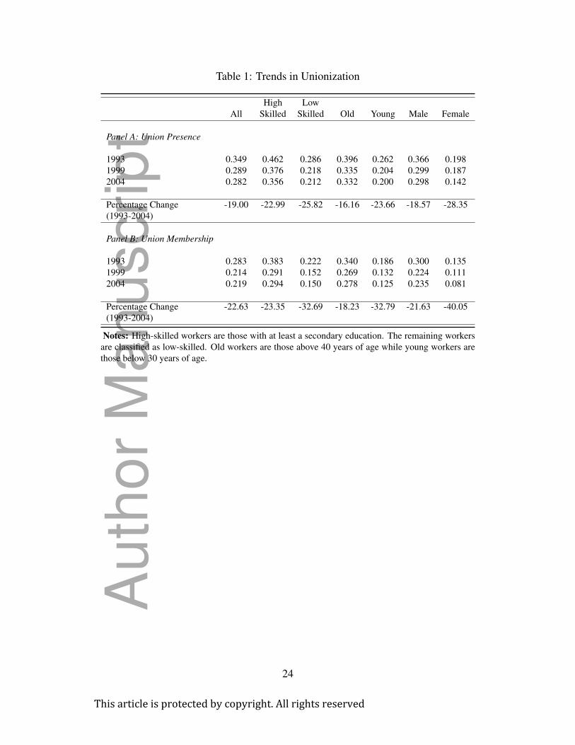
Table 1: Trends in Unionization
High Low
All Skilled Skilled Old Young Male Female
Panel A: Union Presence
1993 0.349 0.462 0.286 0.396 0.262 0.366 0.198
1999 0.289 0.376 0.218 0.335 0.204 0.299 0.187
2004 0.282 0.356 0.212 0.332 0.200 0.298 0.142
Percentage Change -19.00 -22.99 -25.82 -16.16 -23.66 -18.57 -28.35
(1993-2004)
Panel B: Union Membership
1993 0.283 0.383 0.222 0.340 0.186 0.300 0.135
1999 0.214 0.291 0.152 0.269 0.132 0.224 0.111
2004 0.219 0.294 0.150 0.278 0.125 0.235 0.081
Percentage Change -22.63 -23.35 -32.69 -18.23 -32.79 -21.63 -40.05
(1993-2004)
Notes: High-skilled workers are those with at least a secondary education. The remaining workers
are classified as low-skilled. Old workers are those above 40 years of age while young workers are
those below 30 years of age.
24
Thisarticleisprotectedbycopyright.Allrightsreserved
Auth
or
Manuscript

Table 2: Summary Statistics
National Sample Surveys Annual Survey of
(NSSO) Industries (ASI)
Sample Years 1993, 1999, 2004 1993–2004
Level of Industrial Aggregation 3-Digit NIC 1987 2-Digit NIC 1987
Observ- Standard Observ- Standard
ations Mean Deviation ations Mean Deviation
Union Presence 3,361 0.305 0.347 - - -
Union Membership 3,361 0.238 0.321 - - -
Ln(Union Wage) 898 3.980 1.044 - - -
Ln(Adjusted Union Wage) 897 -0.034 0.644 - - -
Output Tariffs 3,361 0.567 0.362 2,625 0.504 0.252
Output NTBs 3,361 0.339 0.307 - - -
Input Tariffs 3,361 0.576 0.360 - - -
Effective Rate of Protection 3,361 0.523 0.452 - - -
Net Importer 3,361 0.445 0.497 2,625 0.602 0.489
Labor Market Flexibility 3,361 0.152 0.747 - - -
Delicensing 3,361 0.804 0.397 - - -
Ln(Quasirents per Plant) - - - 412 8.883 1.317
Ln(Output per Worker) - - - 2,625 6.301 0.806
Ln(Workers per Plant) - - - 2,625 4.066 0.708
Ln(Wage Bill per Plant) - - - 2,625 16.352 2.097
Notes: The union wage, adjusted union wage, and quasirents per plant variables are calculated using
1993 and 2004 data. This is why their sample sizes are smaller. All import protection variables are
lagged by one year. All monetary values above are in 1993 Rupees (Rs.). 1 US dollar in 1993 was
approximately equal to Rs. 31.
25
Thisarticleisprotectedbycopyright.Allrightsreserved
Auth
or
Manuscript

Table 3: Import Tariff Liberalization and Unionization
(1) (2) (3) (4) (5) (6)
Dependent Variable Union Presence Union Membership
Output Tariffs -0.01 -0.05 -0.04 0.04 -0.001 0.01
(0.052) (0.055) (0.055) (0.039) (0.036) (0.037)
Output Tariffs × Net 0.08** 0.09** 0.08** 0.08**
Importer (0.038) (0.039) (0.035) (0.037)
Output Tariffs × Labor -0.004 -0.02
Market Flexibility (LMF) (0.018) (0.015)
Output Tariffs × Net -0.07*** -0.05***
Importer × LMF (0.017) (0.015)
Constant 0.61*** 0.71*** 0.71*** 0.21* 0.30*** 0.30***
(0.170) (0.178) (0.179) (0.109) (0.106) (0.106)
Observations 3,361 3,361 3,361 3,361 3,361 3,361
R-squared 0.564 0.566 0.569 0.562 0.564 0.568
Notes: The dependent variable in columns (1) to (3) is the fraction of individuals in a given
industry, state, and year that work in unionized activities. The dependent variable in columns
(4) to (6) is the fraction of individuals in a given industry, state, and year that are members of
a union. Output tariffs are at the 3-digit industry level and are lagged by one year. The labor
market flexibility measure is from Gupta, Hasan and Kumar (2009). All regressions include
industry-level controls for skill intensity and concentration and industry-state-level controls for
the fraction of casual, household, rural, highly educated, old, and young workers. All regressions
are weighted by the total number of workers in each industry, state, and year cell and include
state, industry, and year fixed effects. Robust standard errors in parentheses are clustered at the
3-digit industry level, *** p<0.01, ** p<0.05, * p<0.1.
26
Thisarticleisprotectedbycopyright.Allrightsreserved
Auth
or
Manuscript

Table 4: Tariff Liberalization and Union Wages
(1) (2) (3) (4) (5) (6)
Dependent Variable Ln(Union Wage) Ln(Adjusted Union Wage)
Output Tariffs -0.34 0.06 0.06 -0.73* -0.55 -0.54
(0.449) (0.434) (0.435) (0.370) (0.381) (0.380)
Output Tariffs × Net -0.73*** -0.72*** -0.35*** -0.37***
Importer (0.143) (0.144) (0.119) (0.124)
Output Tariffs × Labor 0.02 -0.10
Market Flexibility (LMF) (0.068) (0.064)
Output Tariffs × Net 0.02 0.02
Importer × LMF (0.050) (0.056)
Constant 3.54*** 2.28*** 2.28*** 1.11 0.52 0.52
(1.034) (0.702) (0.695) (0.772) (0.666) (0.700)
Observations 898 898 898 897 897 897
R-squared 0.655 0.670 0.670 0.405 0.415 0.419
Notes: The dependent variable in columns (1) to (3) is the average wage earned by union mem-
bers in a particular industry, state, and year. In columns (4) to (6), the dependent variable is the
average wage earned by union members, after adjusting for compositional changes, in a particular
industry, state, and year. Output tariffs are at the 3-digit industry level and are lagged by one year.
All regressions include industry-level controls for skill intensity and concentration and industry-
state-level controls for the fraction of casual, household, rural, highly educated, old, and young
workers. All regressions are weighted by the total number of workers in each industry, state, and
year cell and include state, industry, and year fixed effects. Robust standard errors in parentheses
are clustered at the 3-digit industry level, *** p<0.01, * p<0.1.
27
Thisarticleisprotectedbycopyright.Allrightsreserved
Auth
or
Manuscript

Table 5: The Interdependence of Unionization and Union Wages
(1) (2) (3) (4)
Union Union
Dependent Variable Presence Membership Ln(Adjusted Union Wage)
Output Tariffs -0.15 -0.13 -0.68* -0.64
(0.094) (0.085) (0.394) (0.387)
Output Tariffs × Net Importer 0.12 0.15* -0.18 -0.21
(NM) (0.080) (0.080) (0.164) (0.185)
Output Tariffs × Adjusted 0.05 0.07
Union Wage in 1993 (0.045) (0.041)
Output Tariffs × NM × 0.0004 -0.03
Adjusted Union Wage in 1993 (0.058) (0.049)
Output Tariffs × Union 0.39*
Membership in 1993 (0.230)
Output Tariffs × NM × -0.48**
Union Membership in 1993 (0.233)
Output Tariffs × Union 0.21
Presence in 1993 (0.208)
Output Tariffs × NM × -0.29
Union Presence in 1993 (0.219)
Constant 1.00*** 0.42* 0.73 0.58
(0.239) (0.217) (0.691) (0.643)
Observations 1,084 1,084 830 830
R-squared 0.640 0.676 0.421 0.419
Notes: Adjusted union wage in 1993 is the average composition-adjusted wage in each industry
and state pair in 1993. Similarly, average union membership in 1993 is the fraction of workers in an
industry and state pair in 1993 that were members of a union while average union presence in 1993
is the fraction of workers in an industry and state pair in 1993 that were in a unionized activity. Note
that the interaction between NMi and the average adjusted union wage in 1993 and unionization
in 1993 respectively is time-invariant and is captured by the industry fixed effects. Output tariffs
are at the 3-digit industry level and are lagged by one year. All regressions include industry-level
controls for skill intensity and concentration and industry-state-level controls for the fraction of
casual, household, rural, highly educated, old, and young workers. All regressions include a constant
that is not reported and are weighted by the total number of workers in each industry, state, and year
pair. They also include state, industry, and year fixed effects. Robust standard errors in parentheses
are clustered at the 3-digit industry level, *** p<0.01, ** p<0.05, * p<0.1.
28
Thisarticleisprotectedbycopyright.Allrightsreserved
Auth
or
Manuscript
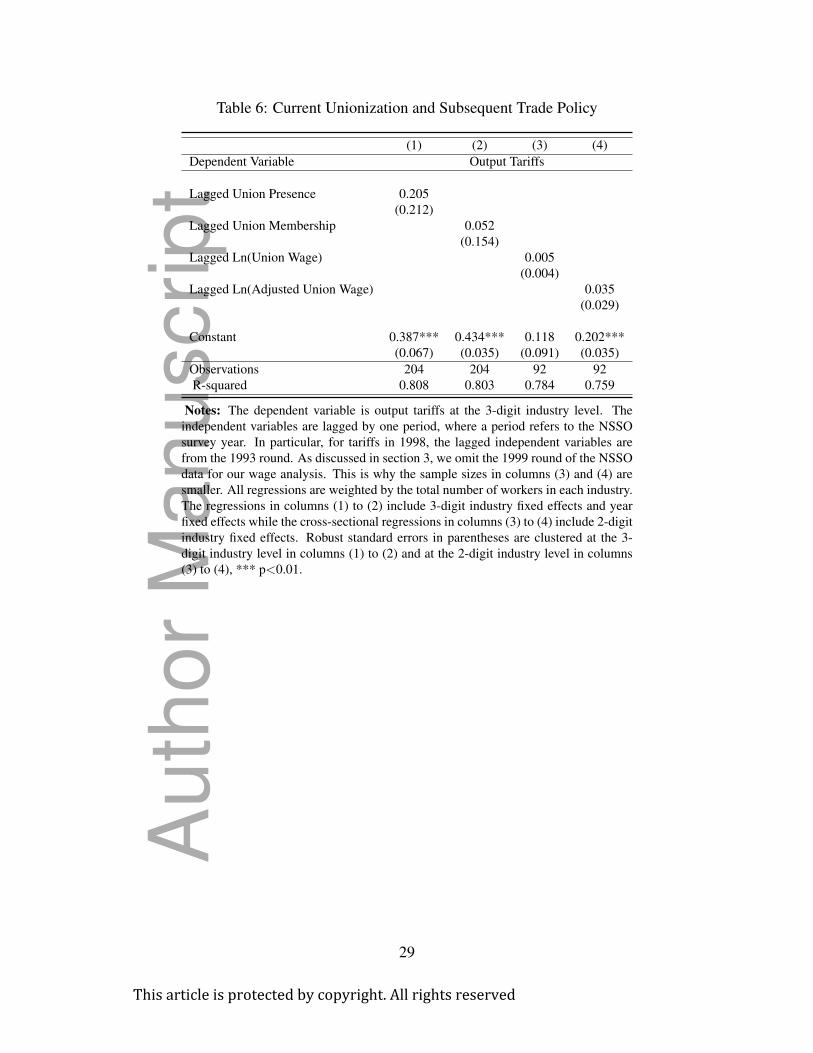
Table 6: Current Unionization and Subsequent Trade Policy
(1) (2) (3) (4)
Dependent Variable Output Tariffs
Lagged Union Presence 0.205
(0.212)
Lagged Union Membership 0.052
(0.154)
Lagged Ln(Union Wage) 0.005
(0.004)
Lagged Ln(Adjusted Union Wage) 0.035
(0.029)
Constant 0.387*** 0.434*** 0.118 0.202***
(0.067) (0.035) (0.091) (0.035)
Observations 204 204 92 92
R-squared 0.808 0.803 0.784 0.759
Notes: The dependent variable is output tariffs at the 3-digit industry level. The
independent variables are lagged by one period, where a period refers to the NSSO
survey year. In particular, for tariffs in 1998, the lagged independent variables are
from the 1993 round. As discussed in section 3, we omit the 1999 round of the NSSO
data for our wage analysis. This is why the sample sizes in columns (3) and (4) are
smaller. All regressions are weighted by the total number of workers in each industry.
The regressions in columns (1) to (2) include 3-digit industry fixed effects and year
fixed effects while the cross-sectional regressions in columns (3) to (4) include 2-digit
industry fixed effects. Robust standard errors in parentheses are clustered at the 3-
digit industry level in columns (1) to (2) and at the 2-digit industry level in columns
(3) to (4), *** p<0.01.
29
Thisarticleisprotectedbycopyright.Allrightsreserved
Auth
or
Manuscript

Table 7: Tariff Liberalization, Unionization, and Union Wages - Mechanisms
(1) (2) (3) (4) (5) (6) (7) (8)
Ln(Quasirents per Ln(Output per Ln(Workers per Ln(Wage Bill
Dependent variable Plant) Worker) Plant) per Plant)
Output Tariffs 0.97*** 1.42** -0.51** -0.05 0.23* -0.16 0.10 -0.27
(0.305) (0.577) (0.232) (0.249) (0.137) (0.141) (0.267) (0.291)
Output Tariffs * Net -0.21 -0.52*** 0.44*** 0.42***
Importer (0.207) (0.104) (0.076) (0.150)
Observations 412 412 2,624 2,624 2,624 2,624 2,624 2,624
R-squared 0.845 0.846 0.848 0.851 0.717 0.723 0.724 0.725
Notes: Output tariffs are at the 2-digit industry level and are lagged by one year. In columns (1) to (2) we use NSSO-
based nonunion wages to construct the dependent variable. Because we only use these data for 1993 and 2004, the
sample sizes in these columns are comparatively smaller. Columns (3) to (8) use annual data between 1993 and 2004.
All regressions include one-year lagged controls for skill intensity and concentration and are weighted by the total
output in each industry, state, and year cell. All regressions also include a constant, industry, state, and year fixed
effects. Robust standard errors in parentheses are clustered at the 2-digit industry-year level, *** p<0.01, ** p<0.05,
* p<0.1.
30
Thisarticleisprotectedbycopyright.Allrightsreserved
Auth
or
Manuscript

Technical Appendix
for
International Trade and Unionization: Evidence
from India
Reshad Ahsan Arghya Ghosh Devashish MitraUniversity of Melbourne University of New South Wales Syracuse [email protected] [email protected] [email protected]
Canadian Journal of Economics
Thisarticleisprotectedbycopyright.Allrightsreserved
Auth
or
Manuscript
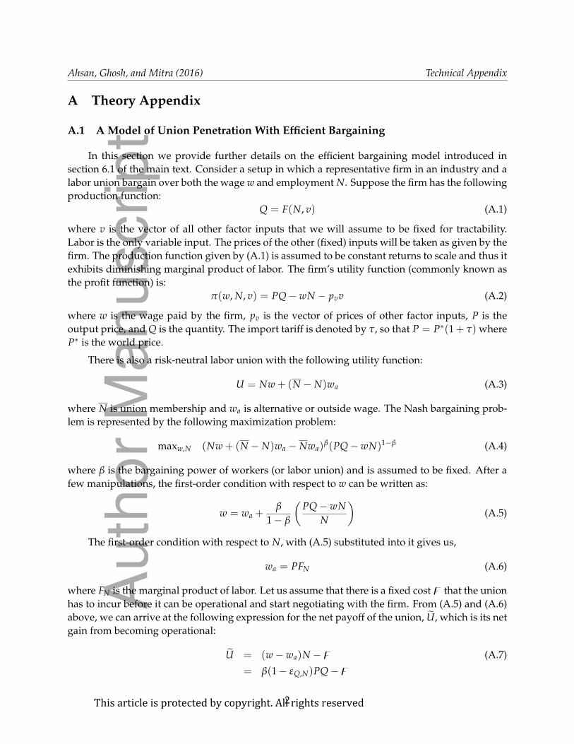
Ahsan, Ghosh, and Mitra (2016) Technical Appendix
A Theory Appendix
A.1 A Model of Union Penetration With Efficient Bargaining
In this section we provide further details on the efficient bargaining model introduced in
section 6.1 of the main text. Consider a setup in which a representative firm in an industry and a
labor union bargain over both the wage w and employment N. Suppose the firm has the following
production function:
Q = F(N, v) (A.1)
where v is the vector of all other factor inputs that we will assume to be fixed for tractability.
Labor is the only variable input. The prices of the other (fixed) inputs will be taken as given by the
firm. The production function given by (A.1) is assumed to be constant returns to scale and thus it
exhibits diminishing marginal product of labor. The firm’s utility function (commonly known as
the profit function) is:
π(w, N, v) = PQ − wN − pvv (A.2)
where w is the wage paid by the firm, pv is the vector of prices of other factor inputs, P is the
output price, and Q is the quantity. The import tariff is denoted by τ, so that P = P∗(1+ τ) where
P∗ is the world price.
There is also a risk-neutral labor union with the following utility function:
U = Nw + (N − N)wa (A.3)
where N is union membership and wa is alternative or outside wage. The Nash bargaining prob-
lem is represented by the following maximization problem:
maxw,N (Nw + (N − N)wa − Nwa)β(PQ − wN)1−β (A.4)
where β is the bargaining power of workers (or labor union) and is assumed to be fixed. After a
few manipulations, the first-order condition with respect to w can be written as:
w = wa +β
1 − β
(PQ − wN
N
)(A.5)
The first-order condition with respect to N, with (A.5) substituted into it gives us,
wa = PFN (A.6)
where FN is the marginal product of labor. Let us assume that there is a fixed cost that the union
has to incur before it can be operational and start negotiating with the firm. From (A.5) and (A.6)
above, we can arrive at the following expression for the net payoff of the union, U, which is its net
gain from becoming operational:
U = (w − wa)N − (A.7)
= β(1 − εQ,N)PQ −
2Thisarticleisprotectedbycopyright.Allrightsreserved
Auth
or
Manuscript

Ahsan, Ghosh, and Mitra (2016) Technical Appendix
where εQ,N = NFN/Q is the elasticity of output with respect to employment of labor. Note that
this is the gain over what these N workers would otherwise get, which is their outside wage. With
a Cobb-Douglas production function, εQ,N is a constant. If, instead, we have a CES production
function of the form,
Q =
[θN N
σ−1σ + ∑
i
θivσ−1
σ
i
] σσ−1
(A.8)
where σ is the elasticity of substitution between any two factor inputs, θN is the weight on labor
and θi is the weight on any other factor input i in the production function, then we have
εQ,N = θN
(N
Y
) σ−1σ
(A.9)
= θσN
(P
wa
)σ−1
The expression above suggests that εQ,N is non-increasing in P when σ ≤ 1 (with σ = 1 being
the Cobb-Douglas case). This condition in turn makes the union payoff from (A.7) unambiguously
increasing in P. Trade liberalization reduces P = P∗(1 + τ) and that in turn reduces the union
payoff.1 Even when σ > 1, we can have U going down with trade liberalization since the effect
of trade liberalization on PQ can counteract the effect on 1 − εQ,N . Note that the union will be in
place only if U > 0. If U is decreasing in P = P∗(1 + τ), then trade liberalization makes union
formation less likely or alternatively, makes deunionization more likely.
To examine the impact of trade on the union wage, we need to substitute (A.6) into (A.5). This
yields
w = wa
[1 + β
(1 − εQ,N
εQ,N
)](A.10)
For a given wa, equation (A.10) suggests that there is an inverse relationship between w and
εQ,N . We know from (A.10) that dεQ,N/dP ≷ 0 if σ ≷ 1. Therefore, trade liberalization will increase
w for given wa when σ > 1 and decrease w for given wa when σ < 1. Another way of stating this is
that w/wa will increase with trade liberalization when σ > 1 and decrease with trade liberalization
when σ < 1. Thus, how trade liberalization will affect the union wage and union-nonunion wage
differential is an empirical question.
1At first, it might seem counterintuitive that in a model with factors other than labor held fixed, the elasticity ofsubstitution has an important role to play. To understand this, suppose we have in the model only two factor inputs,namely labor and capital, and that capital is held fixed. What the elasticity of substitution determines is the responsive-ness of capital intensity (capital-labor ratio) to a change in the wage rate. So for example in the perfect complementscase where the elasticity of substitution is zero, the capital intensity will be fixed (Leontief case). In other words, it isjust the fixed factor that will determine the amount of labor to be used. With σ > 0, as wage goes down the firm willbe willing to use more and more labor and will be less constrained by the amount of the fixed capital it owns (or hasaccess to). If capital and labor are perfect substitutes (σ goes to infinity), the amount of the fixed capital possessed isnot a constraint at all in the firm’s expansion in response to a fall in the wage. In other words, σ tells us how much of aconstraint the fixed factors are for a firm and how easily it can keep adding more labor to expand output as wage keepsfalling.
3Thisarticleisprotectedbycopyright.Allrightsreserved
Auth
or
Manuscript
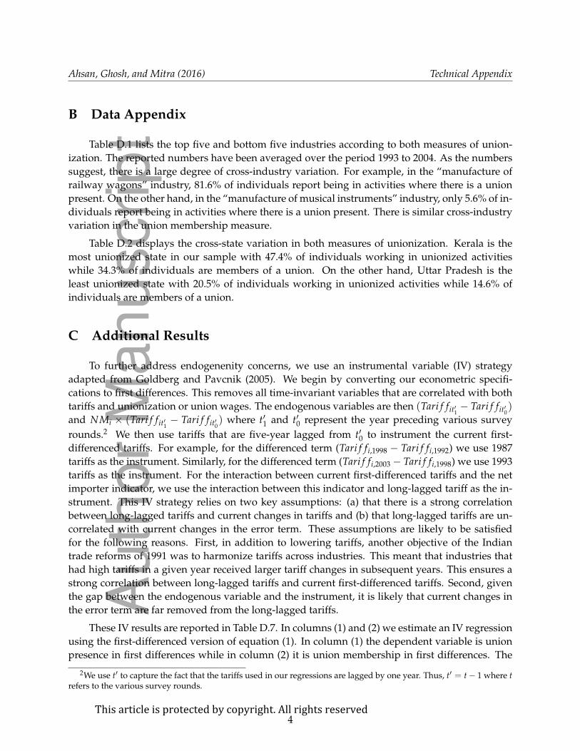
Ahsan, Ghosh, and Mitra (2016) Technical Appendix
B Data Appendix
Table D.1 lists the top five and bottom five industries according to both measures of union-
ization. The reported numbers have been averaged over the period 1993 to 2004. As the numbers
suggest, there is a large degree of cross-industry variation. For example, in the “manufacture of
railway wagons” industry, 81.6% of individuals report being in activities where there is a union
present. On the other hand, in the “manufacture of musical instruments” industry, only 5.6% of in-
dividuals report being in activities where there is a union present. There is similar cross-industry
variation in the union membership measure.
Table D.2 displays the cross-state variation in both measures of unionization. Kerala is the
most unionized state in our sample with 47.4% of individuals working in unionized activities
while 34.3% of individuals are members of a union. On the other hand, Uttar Pradesh is the
least unionized state with 20.5% of individuals working in unionized activities while 14.6% of
individuals are members of a union.
C Additional Results
To further address endogenenity concerns, we use an instrumental variable (IV) strategy
adapted from Goldberg and Pavcnik (2005). We begin by converting our econometric specifi-
cations to first differences. This removes all time-invariant variables that are correlated with both
tariffs and unionization or union wages. The endogenous variables are then (Tari f fit′1− Tari f fit′0
)
and NMi × (Tari f fit′1− Tari f fit′0
) where t′1 and t′0 represent the year preceding various survey
rounds.2 We then use tariffs that are five-year lagged from t′0 to instrument the current first-
differenced tariffs. For example, for the differenced term (Tari f fi,1998 − Tari f fi,1992) we use 1987
tariffs as the instrument. Similarly, for the differenced term (Tari f fi,2003 − Tari f fi,1998) we use 1993
tariffs as the instrument. For the interaction between current first-differenced tariffs and the net
importer indicator, we use the interaction between this indicator and long-lagged tariff as the in-
strument. This IV strategy relies on two key assumptions: (a) that there is a strong correlation
between long-lagged tariffs and current changes in tariffs and (b) that long-lagged tariffs are un-
correlated with current changes in the error term. These assumptions are likely to be satisfied
for the following reasons. First, in addition to lowering tariffs, another objective of the Indian
trade reforms of 1991 was to harmonize tariffs across industries. This meant that industries that
had high tariffs in a given year received larger tariff changes in subsequent years. This ensures a
strong correlation between long-lagged tariffs and current first-differenced tariffs. Second, given
the gap between the endogenous variable and the instrument, it is likely that current changes in
the error term are far removed from the long-lagged tariffs.
These IV results are reported in Table D.7. In columns (1) and (2) we estimate an IV regression
using the first-differenced version of equation (1). In column (1) the dependent variable is union
presence in first differences while in column (2) it is union membership in first differences. The
2We use t′ to capture the fact that the tariffs used in our regressions are lagged by one year. Thus, t′ = t − 1 where trefers to the various survey rounds.
4Thisarticleisprotectedbycopyright.Allrightsreserved
Auth
or
Manuscript

Ahsan, Ghosh, and Mitra (2016) Technical Appendix
coefficients of the interaction term of interest in both columns, while imprecisely estimated, retain
the correct sign. The Shea’s partial R2 in columns (1) and (2) ranges from 0.06 to 0.88. In columns
(3) to (4) we estimate an IV regression using the first-differenced version of equation (3). The
dependent variable in column (3) is the union wage in first differences and in column (4) it is the
adjusted union wage in first differences. Once again, the interaction term of interest retains the
correct sign in both columns. In addition, both interaction coefficient estimates are statistically
significant. The Shea’s partial R2 in columns (3) to (5) ranges from 0.10 to 0.96. Thus, overall, the
IV estimates are qualitatively similar to the OLS results.
Next, in Table D.6 we subject the primary results in this paper to a series of robustness checks.
In columns (1) to (4) the dependent variable is union presence. In column (1) we add a measure of
delicensing to our baseline specification along with its interaction with the net import indicator.
The delicensing measure is an indicator variable that is one for 3-digit industries that have been
delicensed and zero otherwise. This is constructed using data from Aghion, Burgess, Redding
and Zilibotti (2008). Our intention here is to capture the fact that the economic reforms initiated
in 1991 included more than tariff liberalization. Thus, it is possible that these alternate aspects of
the reforms are the primary cause of the subsequent changes in unionization and union wages
in India. However, the results in column (1) suggest that even after controlling for delicensing,
the coefficient of the interaction between output tariffs and the net-import indicator remains pos-
itive and significant. The coefficient of the delicensing variable suggests that industries that were
delicensed experienced a relative increase in union presence.
In column (2) we replace one-year lagged output tariffs with one-year lagged non-tariff bar-
rier (NTB) coverage ratios. The NTB data are from the Asian Development Bank, which is the
same source as the tariff data. As a result, it also covers the period between 1988 and 2003. The
NTB data measures the fraction of products within an industry whose imports were restricted by
non-tariff barriers. As with tariffs, the NTB coverage ratio has also declined dramatically in India
during our sample period. For instance, in the average industry in our sample in 1993, the import
of 66 percent of products within that industry were restricted by NTB’s. In 2004, this number fell
to 6 percent. In fact, the correlation coefficient between industry-level tariffs and NTB’s in our data
is 0.72. As a result of this, our coefficient of interest in column (2) remains highly robust when we
use NTB coverage ratios in place of output tariffs
Next, in column (3) we replace output tariffs with input tariffs in our baseline specification.
The input tariffs were constructed using the output tariff data used in this paper and the 1993–
1994 Indian input-output table in the following way. Consider an industry A that uses inputs from
a number of industries indexed by i. Importantly, A itself may belong in the set indexed by i. This
captures the fact that in most industries in the input-output table, a sizeable portion of inputs are
purchased from within the industry. A’s input tariff is simply the weighted average of the output
tariffs faced by all industries that supply inputs to A. The weights are the share of A’s inputs
that come from each industry indexed by i. The results from using input tariffs in place of output
tariffs are reported in column (3) of Table D.6. As the results show, the interaction between input
tariffs and the net import indicator is positive and statistically significant.
The results in column (3) raises the following question: do output tariffs have an effect on
unionization that is over an above the effect of input tariffs? To examine this, we replace output
5Thisarticleisprotectedbycopyright.Allrightsreserved
Auth
or
Manuscript

Ahsan, Ghosh, and Mitra (2016) Technical Appendix
tariffs in our baseline specification with each industry’s effective rate of protection (ERP). This was
calculated, as in Corden (1969), using the following formula:
ERPit =Tari f fit −
(αjt × InputTari f fit
)
1 − αjt
where InputTari f fit is the input tariff in industry i in year t and αjt is the ratio of the cost of
materials to sales in each two-digit industry.3 Encouragingly, when we use ERP instead of output
tariffs, the interaction between import protection and the net import indicator remains positive
and statistically significant. Further, the results in column (4) suggest that our previous results
cannot be entirely explained by changes in input tariffs. These results indicate that output tariffs
have an impact on unionization that is over and above that of input tariffs.4 We’ve also estimated
an alternate version of columns (1) to (4) with union membership as the dependent variable. These
results are very similar to the ones presented in Table D.6.
In columns (5) to (8) we repeat our robustness checks with the natural logarithm of the ad-
justed union wage as the dependent variable. In column (5) we add our measure of delicensing to
the baseline union wage specification. Once again, the coefficient of the interaction between out-
put tariffs and the net-import indicator remains robust. In column (6) we replace one-year lagged
output tariffs with one-year lagged non-tariff barriers (NTBs). The coefficient of interest again re-
mains highly robust. Finally, in columns (7) and (8) replace output tariffs with input tariffs and the
effective rate of protection respectively. In both cases, the interaction between import protection
and the net import indicator remains negative and statistically significant.
References
[1] Aghion, P., R. Burgess, S. Redding and F. Zilibotti (2008). “The Unequal Effects of Liberaliza-
tion: Evidence from Dismantling the License Raj in India.” American Economic Review 98(4),
1397–1412.
[2] Corden, M. (1969). “Effective Protective Rates in the General Equilibrium Model: A Geomet-
ric Note.” Oxford Economic Papers 21(2), 135–141.
[3] Goldberg, P., and N. Pavcnik (2005). “Trade, Wages, and the Political Economy of Trade Pro-
tection: Evidence from the Colombian Trade Reforms.” Journal of International Economics 66(1),
75–105.
3The α’s were calculated using our industry-level ASI data. Recall that these data are at the 2-digit industry level.As a result, our α’s were also calculated at the 2-digit level.
4Given that industries are classified at a fairly aggregated level in the Indian input-output table, our measure ofinput tariffs is highly correlated with output tariffs. The correlation coefficient between these two variables is 0.97. Asa result of this, we are unable to include both input and output tariffs in the same regression. The advantage of usingERP is that it allows us to account for the changes in both output and input tariffs without facing this multicollinearityproblem.
6Thisarticleisprotectedbycopyright.Allrightsreserved
Auth
or
Manuscript
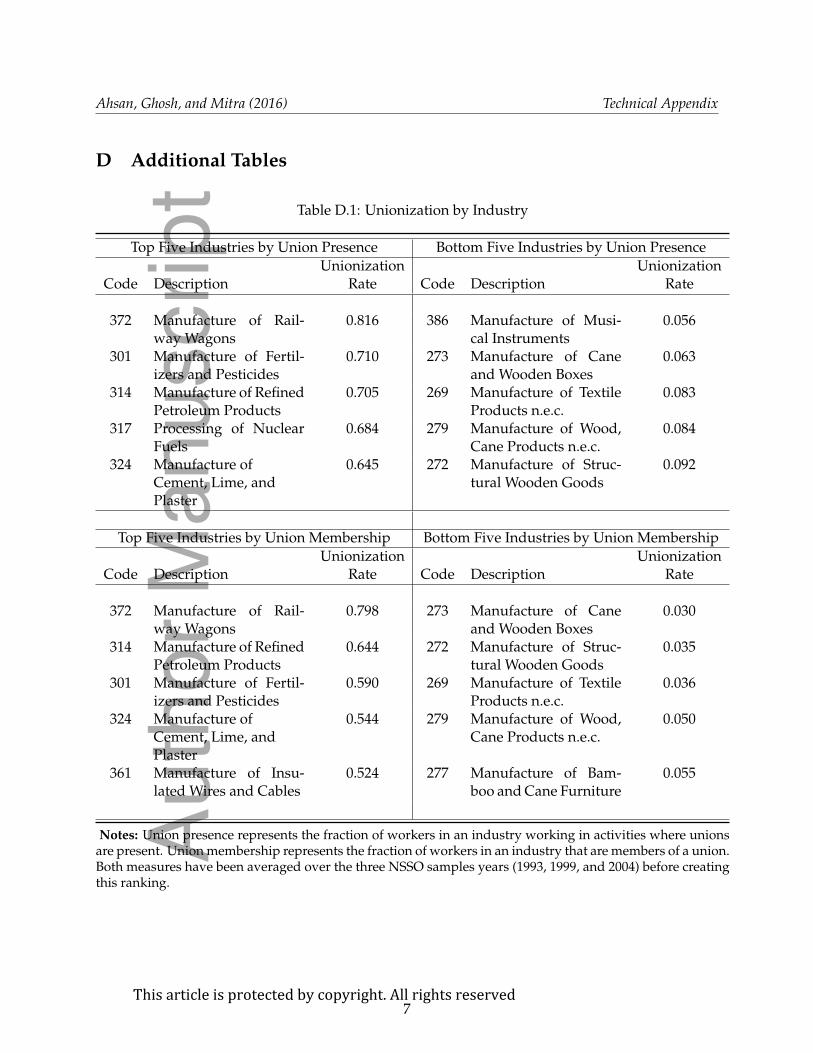
Ahsan, Ghosh, and Mitra (2016) Technical Appendix
D Additional Tables
Table D.1: Unionization by Industry
Top Five Industries by Union Presence Bottom Five Industries by Union Presence
Unionization UnionizationCode Description Rate Code Description Rate
372 Manufacture of Rail-way Wagons
0.816 386 Manufacture of Musi-cal Instruments
0.056
301 Manufacture of Fertil-izers and Pesticides
0.710 273 Manufacture of Caneand Wooden Boxes
0.063
314 Manufacture of RefinedPetroleum Products
0.705 269 Manufacture of TextileProducts n.e.c.
0.083
317 Processing of NuclearFuels
0.684 279 Manufacture of Wood,Cane Products n.e.c.
0.084
324 Manufacture ofCement, Lime, andPlaster
0.645 272 Manufacture of Struc-tural Wooden Goods
0.092
Top Five Industries by Union Membership Bottom Five Industries by Union Membership
Unionization UnionizationCode Description Rate Code Description Rate
372 Manufacture of Rail-way Wagons
0.798 273 Manufacture of Caneand Wooden Boxes
0.030
314 Manufacture of RefinedPetroleum Products
0.644 272 Manufacture of Struc-tural Wooden Goods
0.035
301 Manufacture of Fertil-izers and Pesticides
0.590 269 Manufacture of TextileProducts n.e.c.
0.036
324 Manufacture ofCement, Lime, andPlaster
0.544 279 Manufacture of Wood,Cane Products n.e.c.
0.050
361 Manufacture of Insu-lated Wires and Cables
0.524 277 Manufacture of Bam-boo and Cane Furniture
0.055
Notes: Union presence represents the fraction of workers in an industry working in activities where unionsare present. Union membership represents the fraction of workers in an industry that are members of a union.Both measures have been averaged over the three NSSO samples years (1993, 1999, and 2004) before creatingthis ranking.
7Thisarticleisprotectedbycopyright.Allrightsreserved
Auth
or
Manuscript
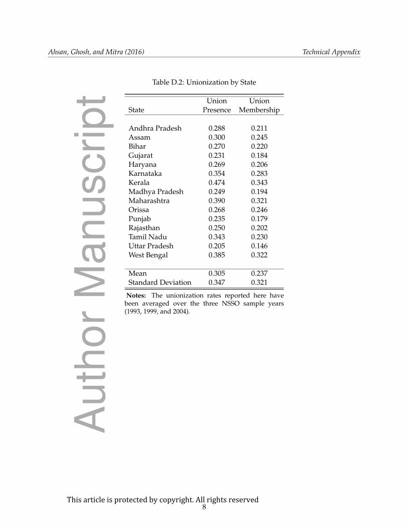
Ahsan, Ghosh, and Mitra (2016) Technical Appendix
Table D.2: Unionization by State
Union UnionState Presence Membership
Andhra Pradesh 0.288 0.211Assam 0.300 0.245Bihar 0.270 0.220Gujarat 0.231 0.184Haryana 0.269 0.206Karnataka 0.354 0.283Kerala 0.474 0.343Madhya Pradesh 0.249 0.194Maharashtra 0.390 0.321Orissa 0.268 0.246Punjab 0.235 0.179Rajasthan 0.250 0.202Tamil Nadu 0.343 0.230Uttar Pradesh 0.205 0.146West Bengal 0.385 0.322
Mean 0.305 0.237Standard Deviation 0.347 0.321
Notes: The unionization rates reported here havebeen averaged over the three NSSO sample years(1993, 1999, and 2004).
8Thisarticleisprotectedbycopyright.Allrightsreserved
Auth
or
Manuscript

Ahsan, Ghosh, and Mitra (2016) Technical Appendix
Table D.3: Alternate Measure of Concentration
(1) (2) (3) (4) (5) (6)
Union Ln(AdjustedDependent Variable Union Presence Membership Union Wage)
Output Tariffs 0.02 -0.01 0.02 -0.01 -0.77* -0.65(0.042) (0.045) (0.036) (0.035) (0.391) (0.408)
Output Tariffs × Net 0.08** 0.08** -0.29**Importer (0.037) (0.035) (0.125)
Constant 0.46*** 0.51*** 0.32*** 0.36*** 1.68*** 1.43***(0.069) (0.076) (0.063) (0.066) (0.486) (0.531)
Observations 3,361 3,361 3,361 3,361 897 897R-squared 0.565 0.567 0.562 0.564 0.407 0.413
Notes: The dependent variable in columns (1) to (2) is the fraction of individuals in agiven industry, state, and year that work in unionized activities. The dependent vari-able in columns (3) to (4) is the fraction of individuals in a given industry, state, andyear that are members of a union. Finally, the dependent variable in columns (5) to (8)is the average adjusted wage earned by union members in a particular industry, state,and year. Output tariffs are at the 3-digit industry level and are lagged by one year.All regressions include industry-level controls for skill intensity and concentrationand industry-state-level controls for the fraction of casual, household, rural, highlyeducated, old, and young workers. Concentration here is defined as the inverse of thenumber of plants in a given industry, state, and year cell. All regressions are weightedby the total number of workers in each industry, state, and year cell. They also in-clude state, industry, and year fixed effects. Robust standard errors in parentheses areclustered at the 3-digit industry level, *** p<0.01, ** p<0.05, * p<0.1.
9Thisarticleisprotectedbycopyright.Allrightsreserved
Auth
or
Manuscript

Ahsan, Ghosh, and Mitra (2016) Technical Appendix
Table D.4: Tariff Liberalization and Unionization: The Role of Individual Charac-teristics
(1) (2) (3) (4) (5) (6)
High LowSkilled Skilled Old Young Male Female
Panel A: Union Presence
Output Tariffs 0.14 -0.07 -0.06 -0.04 -0.05 0.003(0.093) (0.072) (0.075) (0.062) (0.054) (0.183)
Output Tariffs × Net -0.02 0.07* 0.06 0.09* 0.06 0.12Importer (0.062) (0.040) (0.048) (0.045) (0.036) (0.082)
Observations 2,678 2,872 2,485 2,639 3,284 1,549R-squared 0.388 0.483 0.513 0.393 0.563 0.378
Panel B: Union Membership
Output Tariffs 0.19* -0.03 0.08 -0.03 0.01 -0.01(0.099) (0.040) (0.058) (0.039) (0.044) (0.088)
Output Tariffs × Net -0.004 0.07** 0.05 0.13*** 0.06 0.15**Importer (0.069) (0.032) (0.046) (0.040) (0.037) (0.062)
Observations 2,678 2,872 2,485 2,639 3,284 1,549R-squared 0.375 0.467 0.508 0.341 0.533 0.396
Notes: The dependent variable in Panel A is the fraction of individuals in a given indus-try, state, and year that work in unionized activities in various subsamples of the data. Thedependent variable in Panel B is the fraction of individuals in a given industry, state, andyear that are members of a union in various subsamples of the data. High-skilled work-ers are those with at least a secondary education. Old workers are those above 40 yearsof age. Young workers are those below 30 years of age. Output tariffs are at the 3-digitindustry level and are lagged by one year. All regressions include industry-level controlsfor skill intensity and concentration and industry-state-level controls for the fraction of ca-sual, household, rural, highly educated, old, and young workers. All regressions includea constant that is not reported and are weighted by the total number of workers in eachindustry, state, and year cell. They also include state, industry, and year fixed effects. Ro-bust standard errors in parentheses are clustered at the 3-digit industry level, *** p<0.01,** p<0.05, * p<0.1.
10Thisarticleisprotectedbycopyright.Allrightsreserved
Auth
or
Manuscript
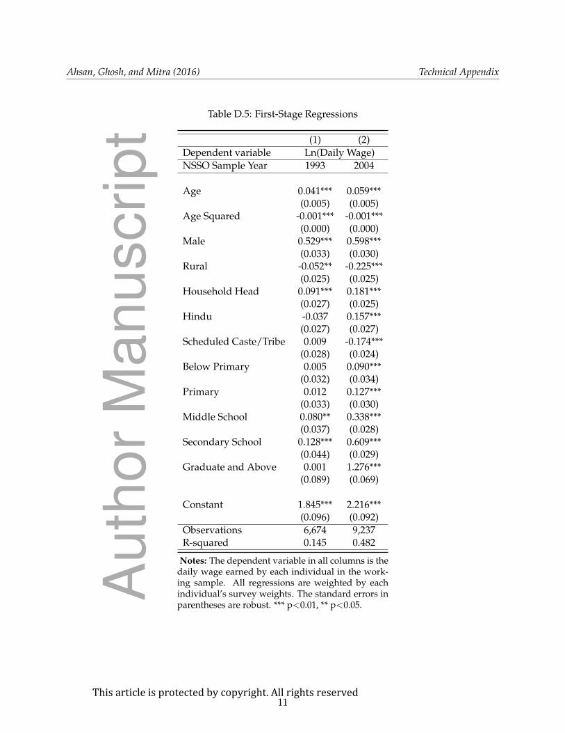
Ahsan, Ghosh, and Mitra (2016) Technical Appendix
Table D.5: First-Stage Regressions
(1) (2)
Dependent variable Ln(Daily Wage)
NSSO Sample Year 1993 2004
Age 0.041*** 0.059***(0.005) (0.005)
Age Squared -0.001*** -0.001***(0.000) (0.000)
Male 0.529*** 0.598***(0.033) (0.030)
Rural -0.052** -0.225***(0.025) (0.025)
Household Head 0.091*** 0.181***(0.027) (0.025)
Hindu -0.037 0.157***(0.027) (0.027)
Scheduled Caste/Tribe 0.009 -0.174***(0.028) (0.024)
Below Primary 0.005 0.090***(0.032) (0.034)
Primary 0.012 0.127***(0.033) (0.030)
Middle School 0.080** 0.338***(0.037) (0.028)
Secondary School 0.128*** 0.609***(0.044) (0.029)
Graduate and Above 0.001 1.276***(0.089) (0.069)
Constant 1.845*** 2.216***(0.096) (0.092)
Observations 6,674 9,237R-squared 0.145 0.482
Notes: The dependent variable in all columns is thedaily wage earned by each individual in the work-ing sample. All regressions are weighted by eachindividual’s survey weights. The standard errors inparentheses are robust. *** p<0.01, ** p<0.05.
11Thisarticleisprotectedbycopyright.Allrightsreserved
Auth
or
Manuscript

Ahsan
,Ghosh,an
dM
itra(2016)
Technical
Appen
dixTable D.6: Robustness Checks
(1) (2) (3) (4) (5) (6) (7) (8)
Dependent Variable Union Presence Ln(Adjusted Union Wage)
Output Tariffs -0.05 -0.54(0.056) (0.382)
Output Tariffs × Net 0.08** -0.35***Importer (0.037) (0.120)Delicensing 0.05*** 0.04
(0.016) (0.263)Output Non-Tariff -0.02 0.38**Barriers (NTB) (0.030) (0.180)Output NTB × Net 0.12** -0.54***Importer (0.050) (0.211)Input Tariffs -0.16 -0.87
(0.133) (1.026)Input Tariffs × Net 0.08** -0.43***Importer (0.038) (0.128)Effective Rate of -0.01 -0.15Protection (ERP) (0.014) (0.107)ERP × Net Importer 0.08** -0.31***
(0.033) (0.107)
Constant 0.71*** 0.62*** 0.80*** 0.67*** 0.51 -0.91* 0.60 0.17(0.170) (0.132) (0.214) (0.149) (0.664) (0.514) (1.061) (0.565)
Observations 3,361 3,361 3,361 3,361 897 897 897 897R-squared 0.567 0.566 0.566 0.566 0.415 0.412 0.411 0.414
Notes: The dependent variable in columns (1) to (4) is the fraction of individuals in a given industry, state, andyear that work in unionized activities. The dependent variable in columns (5) to (8) is the average adjusted wageearned by union members in a particular industry, state, and year. All import protection variables are at the3-digit industry level and are lagged by one year. The delicensing measure is an indicator variable that is onefor 3-digit industries that have been delicensed and zero otherwise. Columns (1) to (4) include all of the controlvariables listed in the body and notes of Table 3. Columns (5) to (8) include all of the control variables listed inthe body and notes of Table 4. All regressions are weighted by the total number of workers in each industry,state, and year cell and include state, industry, and year fixed effects. Robust standard errors in parentheses areclustered at the 3-digit industry level, *** p<0.01, ** p<0.05, * p<0.1.
12Thisarticleisprotectedbycopyright.Allrightsreserved
Auth
or
Manuscript
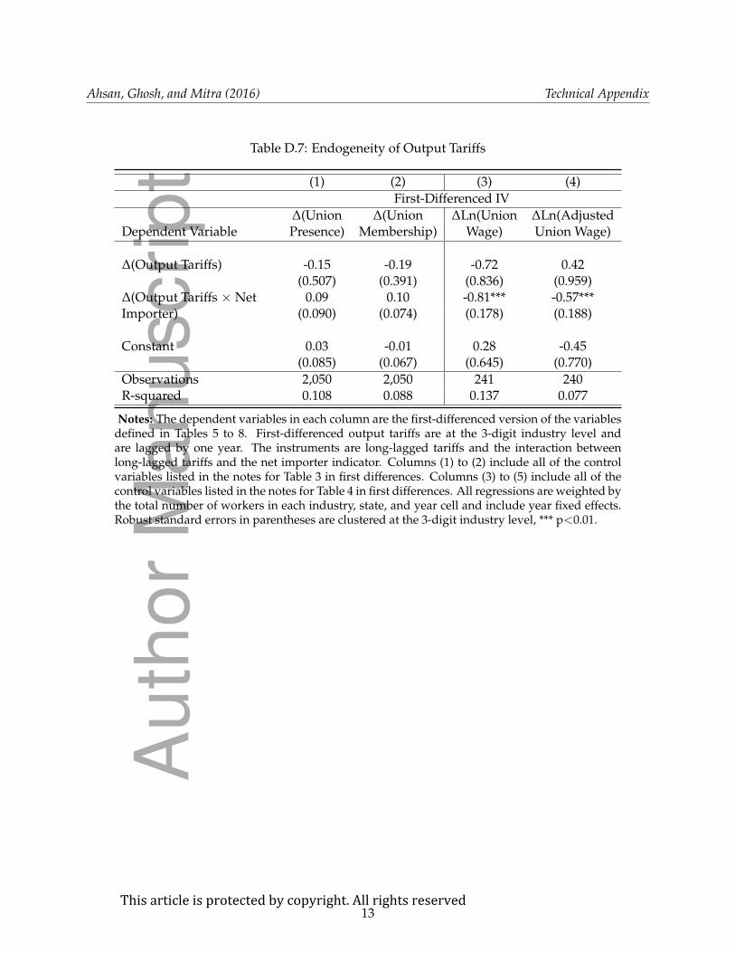
Ahsan, Ghosh, and Mitra (2016) Technical Appendix
Table D.7: Endogeneity of Output Tariffs
(1) (2) (3) (4)
First-Differenced IV
∆(Union ∆(Union ∆Ln(Union ∆Ln(AdjustedDependent Variable Presence) Membership) Wage) Union Wage)
∆(Output Tariffs) -0.15 -0.19 -0.72 0.42(0.507) (0.391) (0.836) (0.959)
∆(Output Tariffs × Net 0.09 0.10 -0.81*** -0.57***Importer) (0.090) (0.074) (0.178) (0.188)
Constant 0.03 -0.01 0.28 -0.45(0.085) (0.067) (0.645) (0.770)
Observations 2,050 2,050 241 240R-squared 0.108 0.088 0.137 0.077
Notes: The dependent variables in each column are the first-differenced version of the variablesdefined in Tables 5 to 8. First-differenced output tariffs are at the 3-digit industry level andare lagged by one year. The instruments are long-lagged tariffs and the interaction betweenlong-lagged tariffs and the net importer indicator. Columns (1) to (2) include all of the controlvariables listed in the notes for Table 3 in first differences. Columns (3) to (5) include all of thecontrol variables listed in the notes for Table 4 in first differences. All regressions are weighted bythe total number of workers in each industry, state, and year cell and include year fixed effects.Robust standard errors in parentheses are clustered at the 3-digit industry level, *** p<0.01.
13Thisarticleisprotectedbycopyright.Allrightsreserved
Auth
or
Manuscript

0 50 100 150 200Average Daily Union Wage (Rs.)
19
93
20
04
Ne
t Impo
rter
Ne
t Exp
orte
r
caje_12263_f1.pdf
Thisarticleisprotectedbycopyright.Allrightsreserved
Au
tho
r M
an
uscrip
t
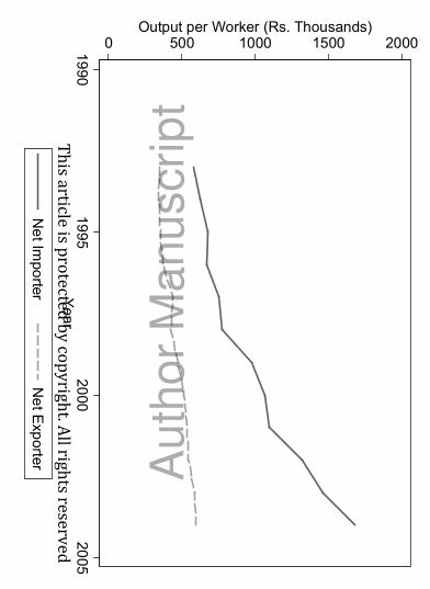
0 500 1000 1500 2000Output per Worker (Rs. Thousands)
19
90
19
95
20
00
20
05
Yea
r
Ne
t Impo
rter
Ne
t Exp
orte
r
caje_12263_f2.pdf
Thisarticleisprotectedbycopyright.Allrightsreserved
Au
tho
r M
an
uscrip
t

Minerva Access is the Institutional Repository of The University of Melbourne
Author/s:Ahsan, RN;Ghosh, A;Mitra, D
Title:International trade and unionization: Evidence from India
Date:2017-05-01
Citation:Ahsan, R. N., Ghosh, A. & Mitra, D. (2017). International trade and unionization:Evidence from India. CANADIAN JOURNAL OF ECONOMICS-REVUE CANADIENNE DECONOMIQUE, 50 (2), pp.398-425. https://doi.org/10.1111/caje.12263.
Persistent Link:http://hdl.handle.net/11343/292832
Related Documents