International - OhioLINK ETD Center

IMwersityMicrofilmsInternational

1.0

l.l

1.25

2.2

“ ■a -“E 1 2.0

1.8

1.4 1.6

'itf

MICROCOPY RESOLUTION TEST CHART NATIONAL BUREAU OF STANDARDS

STANDARD REFERENCE MATERIAL 1010a (ANSI and ISO TEST CHART No. 2)

f.

University Microfilms Inc.300 N. Zeeb Road, Ann Arbor, Ml 48106

INFORMATION TO USERS

This reproduction was made from a copy of a manuscript sent to us for publication and m icrofiim ing. W hile the most advanced technology has been used to pho­tograph and reproduce this manuscript, the quality of the reproduction is heavily dependent upon the quality of the material submitted. Pages in any manuscript may have indistinct print. In all cases the best available copy has been filmed.

The following explanation of techniques is provided to help clarify notations which may appear on this reproduction.

1. Manuscripts may not always be complete. When it is not possible to obtain missing pages, a note appears to indicate this.

2. When copyrighted materials are removed from the manuscript, a note ap­pears to indicate this.

3. Oversize materials (maps, drawings, and charts) are photographed by sec­tioning the original, beginning at the upper left hand corner and continu­ing from left to right in equal sections w ith small overlaps. Each oversize page is also film ed as one exposure and is available, for an additional charge, as a standard 35m m slide or in black and white paper form at.*

4. Most photographs reproduce acceptably on positive microfilm or micro­fiche but lack clarity on xerographic copies made from the microfilm. For an additional charge, all photographs are available in black and w hite standard 35m m slide format.*

*For more information about black and white slides or enlarged paper reproductions, please contact the Dissertations Customer Services Department.

T T-A/F-T Dissertat'°nU ' l v l l Information ServiceUniversity Microfilms InternationalA Bell & Howell Information Company300 N Zeeb Road, Ann Arbor, Michigan 48106

8618767

Couch, Richard Alan

A NEW METHOD TO STUDY TRANSPORT ACROSS MEMBRANES AND INTERFACES USING SPACIALLY RESOLVED SPECTROSCOPY WITH LASER EXCITATION AND DIODE ARRAY DETECTION

The Ohio State University Ph.D. 1986

University Microfilms

International 300 N. Zeeb Road, Ann Arbor, Ml 48106

Copyright 1986

byCouch, Richard Alan

All Rights Reserved

PLEASE NOTE:

In all cases this material has been filmed in the best possible way from the available copy. Problems encountered with this document have been identified here with a check mark V .

1. Glossy photographs or pages ^

2. Colored illustrations, paper or print_______

3. Photographs with dark background ^

4. Illustrations are poor copy_______

5. Pages with black marks, not original copy______

6. Print shows through as there is text on both sides of pag e_______

7. Indistinct, broken or small print on several pages________

8. Print exceeds margin requirements______

9. Tightly bound copy with print lost in spine_______

10. Computer printout pages with indistinct print_______

11. Page(s)____________ lacking when material received, and not available from school orauthor.

12. Page(s)____________ seem to be missing in numbering only as text follows.

13. Two pages numbered . Text follows.

14. Curling and wrinkled pages______

15. Dissertation contains pages with print at a slant, filmed as received__________

16. Other__________________________________ _________________________________________

UniversityMicrofilms

International

A New Method to Study Transport Across Membranes and Interfaces Using Spacially Resolved Spectroscopy

with Laser Excitation and Diode Array Detection

A DissertationPresented in Partial Fulfillment of the Requirements for

the Degree Doctor of Philosophy in the Graduate School of The Ohio State University

by

Richard A. Couch, B.S., R.Ph.

■>V Vr i ’c t'c

The Ohio State University

1986

Dissertation Committee: Approved by

Prof. C.L. Olson Prof. D.D. Miller Prof. R.W. Doskotch Prof. R.W. Brueggemeier

AdviserCollege of Pharmacy

©1986

RICHARD ALAN COUCH

All Rights Reserved

ACKNOWLEDGEMENTS

I wish to express my heartfelt appreciation for the love and encouragement of my parents and family. Without their help this would not have been possible.

My deepest gratitude is extended to Alexa L. Chun for

believing in me and for her help with the hand-drawn fig­

ures .

My sincere appreciation goes to Dr. Carter L. Olson for

his enthusiasm and patience in my work and guidance in my life and career.

I want to thank Salah, Shu-Ling, Hee Kyoung, Paktra,

Anna, Sandy, Sirinart and Jim for all of their help, their

friendship, and for putting up with me in the lab for these past six years.

The technical assistance of, and many helpful discussions with Jack Fowble, Dr. Jagadeesh, and Tom Merrick is grate­fully acknowledged.

Financial support from the College of Pharmacy, The Ohio

State University, the American Foundation for Pharmaceutical Education, and IBM Corporation is especially appreciated.

VITA

January 23, 1957.............. Born: Mason, West VirginiaJan 1978-Aug 1980............. Undergraduate Research

Assistant, College of Pharmacy, The Ohio State University, Columbus, Ohio

June 1980.......................B.S. in Pharmacy, The OhioState University

Sept 1980-Aug 1981........... University Fellow, Collegeof Pharmacy, The Ohio State University

Sept 1981-Aug 1982........... Graduate Teaching Assistant,College of Pharmacy, The Ohio State University

Sept 1982-Aug 1985 ........... Fellow of the Foundation forPharmaceutical Education, The Ohio State University

Sept 1985-Jan 1986........... Research Associate, College ofPharmacy, The Ohio State University

- iii -

CONTENTS

A C K N O W L E D G E M E N T S ............................................... iiV I T A .............................................................iii

Chapter I: Introduction .................................... 1Membrane Transport Measurement History and

Literature Review .................................. 2Spectroelectrochemistry History and Literature

Review ................................................ 6Concentration-Distance-Time Profile Imaging

History and Literature Review ................... 8

Chapter II: Instrumentation: A Laser/Photodiode ArraySpectrophotometer ............................. 11

O v e r v i e w .......................................................11O p t i c s ......................................................... 15

Introduction ........................................... 15A b s o r p t i o n ................................................19D i f f r a c t i o n ............................................... 21Refraction and Reflection ............................. 24Transmittance ........................................... 28

Detection System ........................................... 29Computer Interface and Software ........................ 32

C o m p u t e r .................................................. 32Interface Board ......................................... 33Scan S e q u e n c e r ...........................................34S o f t w a r e ..................................................40

Preliminary Evaluation of Laser/Photodiode ArraySpectrophotometer .................................. 49

Experimental ........................................... 50Results and Discussion ............................... 51S u m m a r y .................................................... 55

Chapter III: Application to an Electrochemical System . 56

T h e o r y ......................................................... 56

- iv -

Chronoamperometry ...................................... 56Concentration as a Function of Position and

T i m e ............................................... 58Spectroelectrochemical Cell Assembly ................... 66

Glass Cell P r e p a r a t i o n : ................................. 71Indicator Electrode Preparation: 74Reference and Auxiliary Electrode Preparation: . . 76Spectroelectrochemical Cell Holder: 77

R e a g e n t s .......................................................83Evaluation of the Electrochemical C e l l .................. 84

Experimental Procedure ............................... 84Results and Discussion ............................... 86S u m m a r y .................................................... 97

Spectroelectrochemical Measurements ................... 97Experimental Procedures ............................... 99Results and Discussion ............................. 101S u m m a r y ................................................... 117

Chapter IV: Application to Studies in MembraneT r a n s p o r t ....................................... 119

T h e o r y ........................................................ 119Nuclepore Membranes .................................... 130Membrane Transport Cell Assembly ...................... 131R e a g e n t s ......................................................140Experimental Procedure .................................. 141

General Procedure .................................... 141Methyl Orange Transport at Different pH Values . 143Methyl Orange Transport Across Nuclepore

Membrane of Various Pore S i z e ................... 144Results and Discussion .................................. 144S u m m a r y ......................................................154

Chapter V: Conclusions .................................... 155

Appendix A: CHRAMP6.BAS .................................. 157

Appendix B: SLAVE.ASM ..................................... 187

Appendix C: LOTFIL.BAS ..................................... 189

- v -

Appendix D: SASFIL.BAS ..................................... 191

Appendix E: CONCPRFL.BAS .................................. 195

Appendix F: C A . B A S .............................................199

Appendix G: MEMTRAN.BAS .................................. 204

Appendix H: THEORMT.BAS .................................. 213

Bibliography ................................................ 217

- vi -

FIGURES

1. A schematic diagram of the laser/photodiodea r r a y .................................................... 12

2. The laser/photodiode array transport measurementsystem.................................................... 13

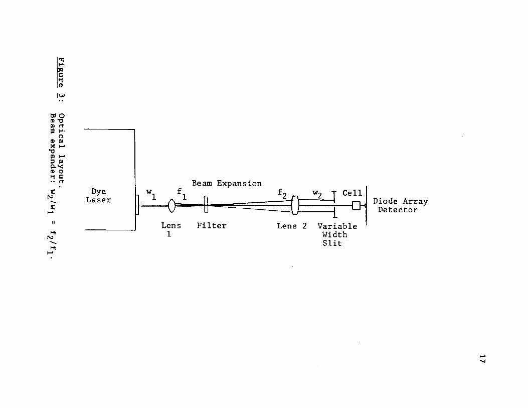
3. Optical layout............................................... 17

4. Effect of distance of a sharp object from thedetector.................................................. 22

5. Wiring diagram for evaluation board connectionto scan sequencer....................................... 35

6. Scan sequencer circuit board design......................377. Wiring diagram for scan sequencer connection to

Tecmar board............................................. 398. Theoretical Concentration Profiles for equal

diffusion coefficients ............................. 639. Theoretical Concentration Profiles for unequal

diffusion coefficients ............................. 6410. Theoretical Concentration Profiles for unequal

diffusion coefficients ............................. 6511. The assembled spectroelectrochemical cell.............. 69

12. The disassembled spectroelectrochemical cell. . . . 81

13. Cyclic Voltammogram of K/^Fe(CN)g........................ 8814. Linear Sweep Voltammograms of KoFe(CN)^ and plot

of i vs. X ............................................. 91

15. (a) Chronoamperogram of K/lFe(CN)g (b) Plot ofApparent Electrode Surface Area as a Function of Time................................................... 95

16. Positional Intensity Measurements of K^Fe(CN)g . 10317. Positional (a) Absorbance and (b) Concentration

K^Fe(CN)g Spectroelectrograms ................... 10418. Spectroelectrograms of K^Fe(CN)g at times 5, 25,

- vii -

108

109

110

112

113

114

115

124

126

127

129

133

136

138

145

147

148

and 65 seconds.Spectroelectrograms of K^Fe(CN)g at times 9, 33,

and 97 seconds....................................Spectroelectrograms of K^Fe(CN)^ at times 17,

65, and 129 seconds..............................

Spectroelectrograms of o-Tolidine at times 1,17, and 65 seconds...............................

Spectroelectrograms of o-Tolidine at times 5,33, and 97 seconds...............................

Spectroelectrograms of o-Tolidine at times 9,49, and 129 seconds..............................

Spectroelectrogram of o-Tolidine at times 257 seconds............................................

Theoretical concentration profiles for transport across a membrane ...............................

Theoretical flux as a function of time fortransport .........................................

(Flux)*( t i m e ) a s a function of time fortransport .........................................

Slope of ( F l u x ) * ( t i m e ) a s a function of time plotted against the square root of diffusion coefficient ......................................

A schematic diagram of the membrane transport cell holder........................................

The membrane transport cell assembly and cell holder..............................................

The disassembled membrane transport cellassembly and cell holder........................

Transport of methyl orange across a Nuclepore membrane .........................................

Flux of methyl orange across a Nucleporemembrane .........................................

Flux * (time)l/^ versus time for the transport of methyl orange ...............................

- viii -

35. Flux of methyl orange at pH 3 .........................15136. Flux * (time)^/^ versus time of methyl orange at

pH 3 ................................................... 152

TABLES

1. Chips Used for the Diode Array Scan SequencerB o a r d .................................................... 36

2. Diode Array Integration Times ........................... 42

3. Comparison of Gilford Spectrometer andLaser/Photodiode Array ............................... 52

4. Absorbance of Fixed Value Neutral Density Filters . . 545. Apparent Electrode Surface Area at Various Scan

Rates Using Linear Sweep Voltammetry .............. 90

6. Correlation Indices of Theoretical andExperimental Concentration Profiles at Various T i m e s ................................................... 107

7. Results of Point by Point Calculation of Dp fromMeasured Concentration ............................. 118

8. Permeation Constants of Methyl Orange at Variousp H s ..................................................... 149

9. Permeations Constants of Methyl Orange forTransport Across Nuclepore Membrane of Various Pore Size.................................................153

- x -

Chapter I INTRODUCTION

The study of species transport across biological and artifi­

cial membranes is important in biopharmaceutics and pharma­

cokinetics. Absorption, distribution and elimination of drugs generally involve movement through one or more mem­branes. This mass transport can take on several forms, but

in general a diffusion layer develops in the solution next

to the interface that separates the phases involved. A dif­fusion layer, or more correctly a boundary layer, is the area in which a concentration gradient forms between two

relatively homogeneous areas. Methods that have been used to study transport have been concerned with measuring the

concentration of the transported species in the bulk solu­

tion away from the interface and the diffusion layer.

The purpose of this research is to develop a new method

to be able to study transport phenomena near interfaces

under hydrodynamically quiet conditions. A new instrument was designed and assembled to accomplish this task. A pro­file of the concentration gradient in the boundary layer itself can be recorded with this instrument.

- 1 -

2The kinds of interfaces of interest include solid/liquid

interfaces, such as an electrode/solution interface, and

liquid/solid/liquid interfaces such as two solutions sepa­rated by a membrane. Because building this instrument

involved a new application of recently developed technology, the first interface studied was to show that the optics and detection system performed properly. The diffusion layer in the solution above a solid electrode provides a theoretical­ly well defined concentration profile that suits this pur­pose well. In another application, transport across a

series of artificial membranes, under a variety of solution

conditions has been characterized. A theoretical model was

developed to aid in the interpretation of these experimental results.

1.1 Membrane Transport Measurement History and Literature

ReviewThe techniques presently employed to study transport across

membranes involve separating two aqueous solutions with the membrane of interest to create donor and receiving compart­ments. The transported species is added to the donor com­partment and one or both solutions are stirred. If the mem­

brane is permeable to the species in question, a boundary layer is established on each side, as molecules of the

species pass into and out of the membrane on both sides of

it. Samples are drawn at pre-determined times from the bulk solution of one or both of the compartments. The concentra­tion of compound in these samples is measured, often spec- trophotometrically, and the change in concentration is

related to the rate of mass transport of that species across the membrane.

These methods developed from experiments first described by Reid in 1901 [1] for the measurement of intestinalabsorption and modified by Wilson and Wiseman [2,3,4]. A

two chamber system [5] and the everted gut sac technique [6]

continue to be used to determine transport across the intes­

tinal wall. Higuchi et al. used a modification of this technique to study permeation of chemical agents through protective skin ointments [7,8]. A similar method has been used to study permeation of drugs and other biologicals through polyethylene and other polymeric membranes [9-14].

With slight variations the same method has been applied to

the measurement of drug permeation through human skin [15,16].

There are disadvantages to these methods. Because of the rather large compartment volume to membrane surface area

ratio used in these techniques, sensitivity is low. A long

time, several hours to more than a day, is required for the concentrations in the two chambers to change enough to pro­vide meaningful and measurable results. For living mem­

branes this may exceed the useful lifetime of the tissue

involved. Also these procedures require manual sampling and

therefore can become quite tedious. To address these prob­

lems, transport measurement cells with a smaller volume to membrane surface area ratio were introduced that use flow

stream methodology for the measurement [17,18,19,20]. These have the added advantage of continuous monitoring of the transport through the membrane. Because of the time

involved in manually taking samples, and the time lag asso­ciated with the flow cell techniques, transient effects on transport can not be measured to the same extent or preci­sion with these methods as with a direct measurement tech­nique. A method that addresses this problem uses an elec­

trochemical detection system with the membrane placed

directly over the electrode surface [21]. This affords both

a small receiving compartment volume and rapid detector

response. However the electrochemical transport measurement

system can not be applied to living membranes because of

their sensitivity to the electrical field produced by the detection system. Also the donor compartment is stirred and the transported species is consumed in the measurement pro-

5In all of the methods discussed, the solution chambers

are stirred to increase the rate of mass transport. This adds another variable to factors affecting transport. The solution hydrodynamics are dependent on the stirring rate,

stirring method, solution volume, and the size and shape of the compartments. These parameters can be difficult to reproduce from one laboratory to another and are not affable to the same rigorous theoretical treatment as a quiet solu­

tion method.

The instrument designed and built as part of this research can measure concentration on one or both sides of an interface in several planes, nearly simultaneously, and

repeatedly without the need for sample extraction or the

resultant sample dilution caused by stirring the sample com­

partments. This direct, non-invasive technique can be used to measure a relatively broad range of transport rates. The

measurement is made very close to the membrane surface (up

to 50 microns) so that quite small compartment volumes can be used (25 microliters or less). Also the system is auto­mated so that there is minimal manual involvement after the initial experimental setup. The solution compartments do not need to be stirred, so that diffusion limited transport can be measured. This makes the experiment easier to repro­duce and theoretically describe. The detector is separated

6from the transport cell in this system, so it can not inter­fere with the transport process.

1.2 Spectroelectrochemistry History and Literature Review As mentioned, the first interface studied was a solid electrode/solution interface. The application of spectro­scopic detection to a species involved in an electrochemical reaction is generally referred to as spectroelectrochemis­

try. The most common application of spectroelectrochemistry involves the use of the optically transparent electrode,

which was introduced by Kuwana in 1964 [22]. This can be

used in the transmission (light perpendicular to the elec­trode surface), internal reflection, or external reflection mode [23,24,25].

In 1974 spectroelectrochemical measurement made parallel to the electrode surface was first reported by Tyson and West [26]. They used a slit to limit the light width and

define the distance from the electrode surface. In subse­quent reports they published crude concentration distance profiles that did not agree well with theory [27,28]. They could measure only up to 250 microns from the electrode sur­

face. Their problems probably resulted from a lack of accu­

racy in measuring the distance from the electrode surface,

diffraction of the light, and most likely solution

7convection in the cell. Another report of the use of a slit in combination with a thin cell and a photomultiplier tube for detection showed somewhat improved results [29,30]. The convection and distance measurement problems were controlled

but diffraction was still a problem. Diffraction due to

both the electrode surface and the slit itself caused sig­nificant deviation from theory.

The first reported use of parallel spectroelectrochemis­try coupled with a diode array detector was in 1983 [31]. The absence of a slit significantly improved the results.

Another report using similar technology appeared in 1985

[32]. The cell used in that study had a 0.15 mm path length. The short path length coupled with the array detec­tor minimizes the effects of diffraction. The work reported

here used at least a 2 mm path length so that the results could be used for comparison to the results in the membrane transport studies. A thin cell is not feasible for membrane

transport measurement because of the edge effects associated

with clamping the membrane between two cell parts. The path

length should be approximately 1 mm or more to minimize this •

edge effect, depending on the membrane thickness. The long­er path length also increases sensitivity. Other attempts to visualize an electrochemical diffusion layer have used

interferometric techniques and have been much more limited in scope [33,34,35,36,37].

81.3 Concentration-Distance-Time Profile Imaging History

and Literature Review Advances in technology have only recently allowed the in- depth study of spatially resolved concentration pattern for­mation in chemical and biological systems. The limiting

factor has been an adequate method of detection. Introduc­tion of solid-state imaging devices and TV-type multichannel detectors have removed this restriction. In a chemical sys­tem where a kinetic process such as a reaction or transfer into another phase is coupled with transport due to convec­

tion or diffusion, both time and spatial resolution of the concentration of the species involved in the process may be

recorded with these detectors.

An early application of this idea has been in the study of flames. Kychakoff et al. reported the time-resolved vis­ualization of reaction zones in laminar flow and turbulent

flames using laser induced fluorescence and a two dimension­

al solid-state photodiode array for detection [38]. The concentration of OH was determined in different reaction zones of the flame under different conditions of combustion.

Muller et al. used a TV camera linked to a computer to study the time-resolved formation of the spiral shaped trav­eling wave of chemical activity of the Belousov-Zhabotinskii

reaction in a thin layer [39]. This is a four step reaction that is catalyzed by ferroin resulting in ferroin/ferriin distribution modulation in the reaction system. Ferroin concentration over a five by five millimeter plane was meas­ured by absorption spectroscopy at three second intervals for two minutes. Color enhanced analysis of this concentra­tion profile revealed Archimedian spirals of chemical reac­

tivity .

Another interesting report used a similar detection sys­

tem to measure intracellular free calcium levels in neutro­

phils during phagocytosis [40]. Fluorescence and a 100X objective lens was used to quantitatively determine the cal­

cium concentration in and immediately surrounding the cell

(approximately 1 mm ). This was used to show that changes in calcium ion concentration are responsible for modulating

certain cell responses.

Two dimensional concentration maps were obtained using a

laser/Vidicon detection system with pulsed and continuous sources for atomic spectroscopy by Steenhoek and Yeung [41].

A laminar flow flame was evaluated for its performance and

the time dependent formation of a laser evaporated plume of

sodium was studied. Two dimensional concentration contours

were reported for these experimental systems.

Because of their non-invasive nature and high information content, research using these sophisticated techniques to determine concentration as a function of position and time in physicochemical and biological systems is expected to

grow in the future.

Chapter IIINSTRUMENTATION: A LASER/PHOTODIODE ARRAY

SPECTROPHOTOMETER

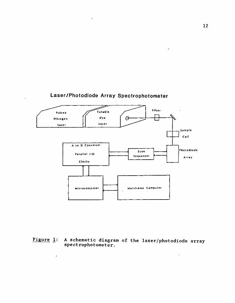
2.1 OverviewThe experimental system used in these studies is depicted schematically in Figure 1 and is pictured in Figure 2. The detection is based on absorption spectroscopy. A tunable

dye laser, pumped by a pulsed nitrogen laser, is used to

provide a source of highly monochromatic, parallel light of

a selected wavelength. The light is filtered to decrease its intensity to the desired level and the diameter of the

beam is expanded with a set of lenses. The beam is directed through a slit and then the sample cell which houses the

system being studied. A photodiode array arranged orthogo­nal to the interface and beam serves as the detecting unit.

All of this sits on a floating optical table to isolate it from room vibrations. A dedicated microcomputer controls

the laser directly and the diode array through a scan sequencer. The microcomputer is linked to a mainframe com­puter through an RS232 asynchronous communication line and a

coaxial cable.

- 11 -

12

Laser/Photod iode Array Spectrophotometer

F i l l e rT u n a b leP u ls e d

D y eN i t r o g e n

L a ie rl a s e r

C e l l

P h o t o d i o d e

A r r a y

Scan

S e q u e n c e r

M i c r o c o m p u t e r

P a r a l l e l I / O

C lo c k s

M a in f r a m e C o m p u t e r

Figure _lt A schematic diagram of the laser/photodiode array spectrophotometer.

13

Figure 2: The laser/photodiode array transport measurementsystem.

I A Q F R

152.2 Optics

2.2.1 IntroductionThe lasers are a Molectron model UV-22 pulsed nitrogen las­

er, which provides light of wavelength 337.1 nm, and a Molectron model DL-II (DL-14) tunable dye laser (Molectron Corporation, Sunnyvale, California; presently Cooper Laser- onics). The dye laser is wavelength selectable from 360 to 950 nm, fundamental and down to 217 nm frequency doubled,

with a linewidth of 0.01 nm. The external trigger of the

nitrogen laser is connected to an output clock of the com­

puter interface system with a coaxial cable. Only the

oscillator cell of the dye laser was used in most of these

studies, as it provided more than enough light power to sat­urate the detector.

The laser beam is filtered with either a combination of

neutral density filters or a solution of a species that absorbs the wavelength being used. The beam diameter is about 2.5 mm and has a gaussian cross-section. In order to maintain the parallel property of the light while increasing the diameter of the beam, two convex lenses are arranged as shown in Figure 3. The beam first passes through the short

focal length lens, causing it to converge. The second lens

recollimates the light. The beam expansion achieved is giv­

en b y :

16w 2 /v?i = ^ 2 ^ 1 etJ* ^ - 1

This arrangement is a simple refractor telescope in reverse [42]. The lenses used have focal lengths of 4.06 cm and

34.54 cm. The beam expansion achieved was from 0.25 cm to 2.15 cm, which is large enough for the sample cell and detector. Even at this diameter the gaussian nature of the beam is evident (see Figure 4a). The expanded beam is then directed through a variable width slit to decrease the pos­sibility of stray light reaching the detector from the

sides. In particular, reflections from the rounded outsides

of the square bore glass tubing used in the various sample

cells must be eliminated. Decreasing the beam width so that it is more narrow than the inside diameter of the square

bore glass tubing accomplishes this. The adjustable width slit also provides another means of controlling the total power input from the incident beam.

The most important property of a laser that makes it ideal for this study is the collimation of the light [43,44,45,46]. For any study involving positional absorp­

tion measurements, control over light collimation is criti­cal . The second lens of the beam expander was fine adjusted

such that the diameter of the beam was exactly the same a few centimeters away and a few meters away, as measured with

H-TOCnnlu>

w o 0) *0 Pi rT3 H- oro pi x i-> TJpi t-* 3 Pi avjrp o h c• • rT

t 'Ni

IIHiN>H i

DyeLaser

Lens1

Beam Expansion

Filter

Cell

Lens 2 VariableWidthSlit

Diode Array Detector

a vernier caliper. This is a difficult measurement to make

since the edges of the beam are not very sharp. The speci­

fication for the dye laser is for a divergence of 1 mRadian

[47]. A beam that had a diameter of 3190.00 microns at a given distance (in this case, the cell) with a divergence of 1 mRadian, would have a diameter of 3200.00 microns at a

distance 1 cm further away (at the detector). Assuming that

the center of the laser beam is perpendicular to the diode in the middle of the array, the light that passed through the cell 800 microns away from the center of the beam would fall on the diodes 802.5 microns away from the center of the array. Similarly the diodes at the very edge of the array (1600.0 microns from the center) would receive light that had passed through the cell at 1595.0 microns from the cen­

ter of the beam. Therefore for a 1 mRadian divergence, the

diodes at the edge of the array are spatially off by 5

microns (out of its 25 micron height) in the vertical direc­

tion only. The divergence is in all directions, but only the vertical divergence is of any importance here. For the sloping curves of a concentration gradient this is a small

error.

The laser beam transverses the sample cell, which houses the interface under investigation. Design and characteris­tics of the individual sample cells are discussed in the

19next two chapters. The optical radiation can interact with the media of the cell in several ways, including absorption, transmission, reflection, refraction, and diffraction

[48,49,50]. The possible effects of each of these must be taken into account to fully interpret the spectral results.

2.2.2 AbsorptionAbsorption results in transferring the energy of electromag­netic radiation to the absorbing media. The absorbing mol­ecules are excited to a higher energy state. Relaxation

back to ground state can occur by several processes, one of

which is a non-radiative loss of energy in small steps by

collisions with other molecules. The energy is converted to kinetic energy, resulting in a minute increase in the temp­erature of the system. Therefore, the possibility of heat­

ing the solution in the sample cell, resulting in thermal convection, must be considered. With a nitrogen laser pulse

width of 10 nanoseconds, the dye laser has a nominal pulsewidth of 6-8 nanoseconds. So for a pulse rate of 10 Hz thelaser beam is actually interacting with the sample solution

Oonly 6-8 x 10 percent of the time. The energy conversion efficiency of the dye laser using only the oscillator cavity is approximately 6 percent (this can be increase to 15 per­

cent when the amplifier cell is added). The pulse energy of

the nitrogen laser is 0.006 joules [47,51]. Therefore the

20pulse energy of the dye laser is 3.6 x 10~^joules. This isthen neutral density filtered with 1.0-2.0 O.D. filters,removing at least 90 percent of the light, resulting in anoutput of 3.6 x 10”^joules per pulse. A slit is also usedwhich selects a small portion of the beam to actually pass

through the sample solution. Generally this removes at

least another 90 percent of the beam, since the expandedbeam is 2.2 cm and the slit is open less than 0.2 cm. This

- 6decreases the incident light to 3.6 x 10 joules per pulse. For an experiment where a large amount of information is

collected over a relatively short time, at most 10 pulses, every other second for up to 200 seconds (1000 pulses total)

could be used. This is the most energy reaching the solu­

tion per time, providing 0.0036 joules or 0.00086 calories over 3.33 minutes. Assuming that every bit of this is absorbed by the solution and the solution heat capacity is 1 cal/gm°C, for a 0.1 ml solution volume, the total tempera­ture increase would be 0.0086°C. For a short experiment

this is not enough temperature difference to cause convec­

tion. For longer experiment, more total pulses may be used

(up to 3000), but these are spread out over much longer time

periods (more than 2 hours), giving more than adequate time

for any temperature differences in the solution to non-

convectively dissipate. The temperature rise is less than

210.000172°C per minute in these longer experiments. It

should be pointed out that a continuous light source would

heat the sample solution many times more.

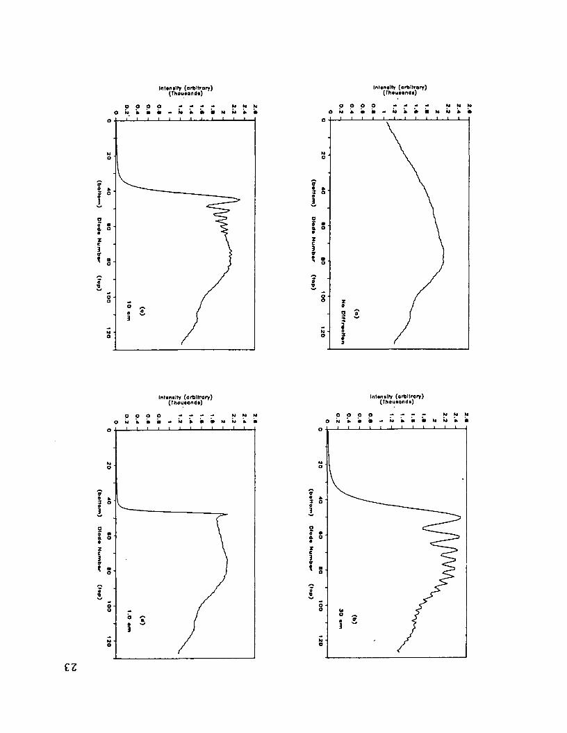
2.2.3 DiffractionThe phenomena of diffraction must also be dealt with in any attempt to make positional intensity measurements. Diffrac­

tion is the bending of waves around the edge of an object as a consequence of interference [49,50]. This is demonstrated in Figure 4. In this experiment the laser beam was directed over a horizontal razor blade with the blade pointing up. The diffraction pattern this creates resembles a decaying sine wave. The intensity maxima are due to constructive

interference and the minima are due to destructive interfer­

ence. As is demonstrated in the figure, both intensity and

vertical distance above the edge of the razor of the waves

decrease as the object is moved closer to the detector.

Therefore, in order to minimize the diffraction effects, the sample cell was moved as close to the detector as possible.

The distance of 1.0 cm in Figure 4(d) represents the dis­tance from the detector to the leading edge of the interface in a typical experiment. At this distance it appears that information is significantly affected in only one or two diodes, representing a distance of 25-50 microns. This is the limit of the measurement system in terms of closeness to

the interface.

22

Figure 4: Effect of distance of a sharp object from thedetector.Lambda = 400 nm.(a)Full scale light, no diffracting body. Diffractive pattern due to a horizontal razor blade edge at (b) 30 cm, (c) 10 cm, (d) 1.0 cm. The diodes have a center to center spacing of 25 microns.

40 00

80 100

120 0

20 40

60 80

10O

12

0

(bo

ttom

) O

todo

Num

bor

(top)

(bo

ttom

) D

lodo

Num

bor

(top

)

In fin a lty (o rb ttro ry )(Thouaanda)

O O O O - - - - M M MO N

o

NO

I n t im ity (o rb itrq ry ) (Thouaond i)

O O O O - - - - M M MO N * i » • - w * 2» • n m W •

o

No

o

o

9o

oo

No

In t im ity (a rb itra ry ) (T h o u ia n d i)

O O O O N U NO N W d i a ~ M b

In t im ity (a rb itra ry ) (Thouaond i)

O O O O - - - - U M MO N fr • 9 - N * • ■ M M * m

o

too

*o

o

■o

oo

Mo

ez

242.2.4 Refraction and ReflectionAnother possible interaction of light with matter that should be addressed is the phenomena of refraction. Refrac­tion is the change in direction of light that is observed

when it passes from one medium to another. This is due to

the difference in the velocity of the radiation in the two media. The refractive index n^ of a substance is the ratio of the velocity of light in a vacuum to the velocity of

light in the substance. The angle of refraction of between

two media is given by Snell's law of refraction:

sin 0^/sin 02 = = v^/v£ eq. 2-2

where 0- is the incident angle of the light away from normal to the media, 0£ is the resultant angle away from normal, and v^ is the velocity of light in the media, 1 and 2. In

these experiments the light beam is directed normal to the cell, meaning incident angle, 0- , is zero and therefore

regardless of the refractive indices of the two media

involved, the resultant angle of refraction between them is also zero.

Another light/matter interaction that occurs when light

passes from a medium of one refractive index to a medium of different refractive index is reflection. For a beam trav­

eling normal to the surface of the media it is transversing,

reflection is in the same plane as the impinging beam and is given by:

where IR is the reflected intensity, Iq is the incident

intensity and n^ are the refractive indices of the two media[49,52]. The fraction reflected can be calculated usingthis. In subsequent calculations assume na^r is 1.0003,

nglass 1*500, and ignore any effect of multiple reflec­tion (difference of less than 0.2 percent [52]). The

refractive index of double distilled water, measured with an Abbe refractometer (Bausch and Lomb, Rochester, N.Y.), was found to be 1.3325 at 589 nm, corrected to 20°C [53]. For the four surfaces the light passes (air to glass, glass to solution, solution to glass, and glass to air), the fraction

reflected is calculated to be 0.086879 . The actual frac­

tion reflected is not important in a relative measurement

however. It is the change in fraction reflected as the

solution composition changes in a given experiment that must

be considered. Fortunately the difference is very small. In the electrochemical experiments the change is exception­ally small, since the change is due to the difference in

refractive index of different oxidation states of the same

(n2 -n i)2eq. 2-3

(n2+n1 )2

26species. For example, for the oxidation of o-tolidine to the quinonediinline, the change in refractive index is less

than 0.0001. The change in fraction reflected for a differ­ence of 0.0001 (n=1.3346 to 1.3347) would be 0.000008(0.086694-0.086686). For an experiment in which the solu­tion composition changes more radically, for example from

distilled water to 0.1 M KCl (n=1.3342) the change in frac­tion reflected is 0.00015 (0.086879-0.086729), which isstill much smaller than the margin of error in these experi­ments .

Refraction can also occur within a media, if the media does not have a homogeneous refractive index. This is the

principle upon which gradient index lenses are based. Where

there is a concentration gradient in a solution there may

also be a refractive index gradient which will tend to bend the light in the direction of the higher refractive index. The steeper the refractive index gradient of the media, the shorter the radius of curvature of the light path [54]. The

vertical curvature of a light beam proceeding perpendicular

to a refractive index gradient is given by:

3y = L in eq 2-4J n 3y

where 3y is the angle of deflection in the y direction, L is the path length of the light and (3n/3y) is the vertical

27refractive index gradient. If a large gradient formed, such

as from 0.1 M KCl (n=1.3342) to distilled water (n=1.3325), a significant bending of the beam would occur. For L=.002 meters, 3n = .0017, 8y = .0032 meters and using and average refractive index for n (1.33335), 3y is 7.969 x 10"®^ Radi­ans or .04566°. In addition, when this light passes to the glass the angle decreases slightly to .04058° and when it

passes back to the air the angle increases to 0.06087° due to refraction. Shifts of this size should not significantly

affect the results. Fortunately the actual refractive index

gradients are not that large. In the electrochemical exper­iments large concentration gradients are formed, however the refractive index gradients are very small. This is because,

as the reacting species diffuses to the electrode surface, the product, which has a nearly identical refractive index,

diffuses away, forming an exactly opposite concentration gradient, if the two diffusion coefficients are the same. The difference between the refractive indices of the two oxidation states of o-tolidine is too small to measure with an Abbe refractometer (less than 0.0001). In the membrane

transport studies, the potential for a significant refrac­

tive index gradient is greater. However, the refractive

index of the solutions of compounds used and the buffers

used for preparing them is also the same to four places

28passed the decimal. For example, borate buffer, pH = 10,ionic strength = 0.1, has a refractive index of 1.3327. A

_ *3solution of 10 molar 4-nitrophenol dissolved in this buff­

er has the same measured refractive index. The buffers used

to prepare the solutions of absorbing species are always

used as the background solutions in the membrane transport study cells. If the refractive index gradient were 0.0001 units the total angle change from the incident beam (includ­ing passing through the glass and air would only be .00358°

or 6.25 xlO"'* Radians, a very small deflection. When making

membrane transport measurements, the refractive indices of the two solutions used (the background solution and the introduced solution) should be measured and the refractive

index difference minimized to account for this effect.

2.2.5 TransmittanceTransmittance is defined as the fraction of the incident

light that passes through the cell. Changes in transmis­

sion, due to absorption, result in the useful analytical

signal. Absorbance, A, is defined as:

A = -log10T = -log10(P/Po ) eq. 2-5

where T is the transmittance, P is the power of the passed

light and PQ is the power of the incident beam, both cor­

rected for dark current.

29Absorbance is related to concentration by the expression:

A = ebC eq. 2-6

which is Beer's Law (or the the Beer-Lambert Law), where c

is the molar extinction coefficient, b is the cell path

length in cm and C is molar concentration. Combining these two equations the concentration of a species whose molar

absorbance is known can be calculated from intensity meas­urements .

2.3 Detection SystemThe detecting unit is a solid state self-scanning linear

photodiode array (RL-128S, Reticon Corporation, Sunnyvale, California) [55,56,57]. The detector chip contains 128 pho­todiode sensor elements in a 3.2 mm height for simultaneous light intensity measurements in 128 planes with a center-to-

center spatial resolution of 25 microns. The sensor ele­

ments are 2.5 mm wide. A photodiode outputs a charge pro­

portional to the exposure of light it receives (intensity times integration time). A photodiode is a silicon wafer

with a p-n junction operated in a reverse bias mode. When the appropriate radiation impinges on the junction, hole- electron pairs are formed causing a current to flow [58,59]. A good review of the use of diode array detectors in spec­

troscopy has recently been published [60,61].

30The photodiode array chip is mounted on an evaluation

board (RC-1024SA, Reticon). The program logic to process

the diode array's immediate signal is provided by this eval­

uation board. This printed circuit board controls the inte­gration time of the array, supplies the clocks, and partial­

ly processes the image signal from the array chip [62]. The diode array and evaluation board are housed in a 3 x 5 x 10 inch aluminum chassis (BUD cat. no. AC-404) fitted to accom­

modate the 44 pin holder. The center of the pin holder is

1.2 cm from the front edge of the housing. A 3 by 8 inch section of the front of the housing was removed to allow maximum access to the diode array. With this design a sam­ple cell holder could be placed nearly against the detecting unit, getting the sample cell itself to within a centimeter of it. The pin holder is wire-wrap connected to an edge pin

connector on the side of the chassis. The back plate of the

box was fitted with a 2.5 inch diameter, 3 inch long flexi­

ble hose attached to a fan. Air is pulled through the box

to cool the evaluation board without introducing vibrations

from the fan into the system being studied. The box was spray painted matte black and the back plate was coated with black felt to decrease the introduction of stray light to

the detector.

31The clock frequency of the evaluation board is adjustable

to operate between 150 KHz and 1.5 MHz. This corresponds to

a data collection rate of 38.5 to 386 KHz, since each diode output cycle requires four clock pulses to sample and reset

each diode's capacitor. Experiment has shown that data col­lection at 100 Khz, an oscillator frequency of 400 KHz, gives much better results than slower data collection (par­ticularly under 50 KHz). The slower rates show a more pro­nounced odd-even disparity over at least half of the video output range, getting worse at higher light intensities. The odd-even disparity can be largely eliminated over a

range of up to 90 percent of the saturated video output at a

data collection frequency of 100 KHz. The evaluation board was modified to allow software selectability of the integra­tion time through a parallel I/O line of the microcomputer.

The integration time can be set from 2.7 to 300 mSec. In order to easily synchronize with the laser pulsing and mini­

mize the dark current, an integration time of 5.0 msec was

found to be most practical.

The evaluation board also partially processes the video signal. The odd and even diode signals are independently pre-amplified and then multiplexed into one signal. There are five outputs from the evaluation board: (1) the multi­plexed video output (0-3 volts), (2) scan start, (3) odd

32end-of-line, (4) even end-of-line, and (5) the oscillator clock. Complete timing diagrams, board layout, and operat­ing instructions for the RC-1024SA evaluation board can be found in reference [62].

2.4 Computer Interface and Software

In order to accomplish the complex timing involved with this system and to handle the large amount of data generated, the

laser and photodiode array are interfaced to a dedicated microcomputer. An IBM PC-XT and PC-AT (IBM Corp., Boca Raton, FI.) have been used with a Tecmar PC-Mate LabMaster

data acquisition subsystem (Tecmar Inc., Cleveland, Ohio).

Initial processing of the diode array video signal is accom­

plished by a separate circuit board called a scan sequencer,

through which the computer controls the diode array and can collect the video data. Software has been developed to set

up and coordinate the tasks necessary to run and evaluate an experiment.

2.4.1 ComputerOriginally an IBM Personal Computer XT equipped with a disk­

ette drive, fixed disk, printer, monochrome and color dis­

plays, asynchronous communications adapter and interface

board was used to collect and process the experimental data.

The spectroelectrochemical results, presented in Chapter

33III, were obtained using this computer. Data could be col­

lected under program control at a maximum 52,000 points per second. This system worked well, but the computer's data collection rate was the limiting factor. The analog to digital converter of the Tecmar board is capable of rates up to 100,000 points per second and the diode array can gener­ate data at over 300,000 points per second. The IBM PC-AT was similarly equipped and could collect data at the limit­

ing rate of the analog to digital converter, 100,000 points

per second, using the same software with minor adjustments.

The membrane transport experiments of Chapter IV were done with this computer. Advantages of faster data collection speed were discussed in section 2.3 .

2.4.2 Interface Board

The Tecmar LabMaster data acquisition subsystem consists of a mother board, which plugs into the PC bus and a daughter board, which is housed separately. The mother board con­tains circuitry for two independent 12 bit resolution digi­tal to analog (D/A) converters, five independently program­mable 16 bit timer/counters and three 8 bit parallel ports.

The daughter board contains a multiplexed 16 channel, 12 bit

resolution analog to digital (A/D) converter. The daughter

board has been modified to contain all of the functions and

controls of the mother board using ribbon cable, edge

34connectors, and BNC connectors. The Tecmar board is set up in the input/output (I/O) mapped mode and + /- 10 volts full scale A/D input. The board is controlled by outputting the proper bit patterns to the assigned port addresses for the various functions [63].

2.4.3 Scan Sequencer

The scan sequencer board contains the power supplies for the diode array's evaluation board, adjusts the video output, and provides a clock signal to be compatible with the Tecmar

LabMaster interface board. The evaluation board has a 22

lead dual in-line edge connector. This communicates with

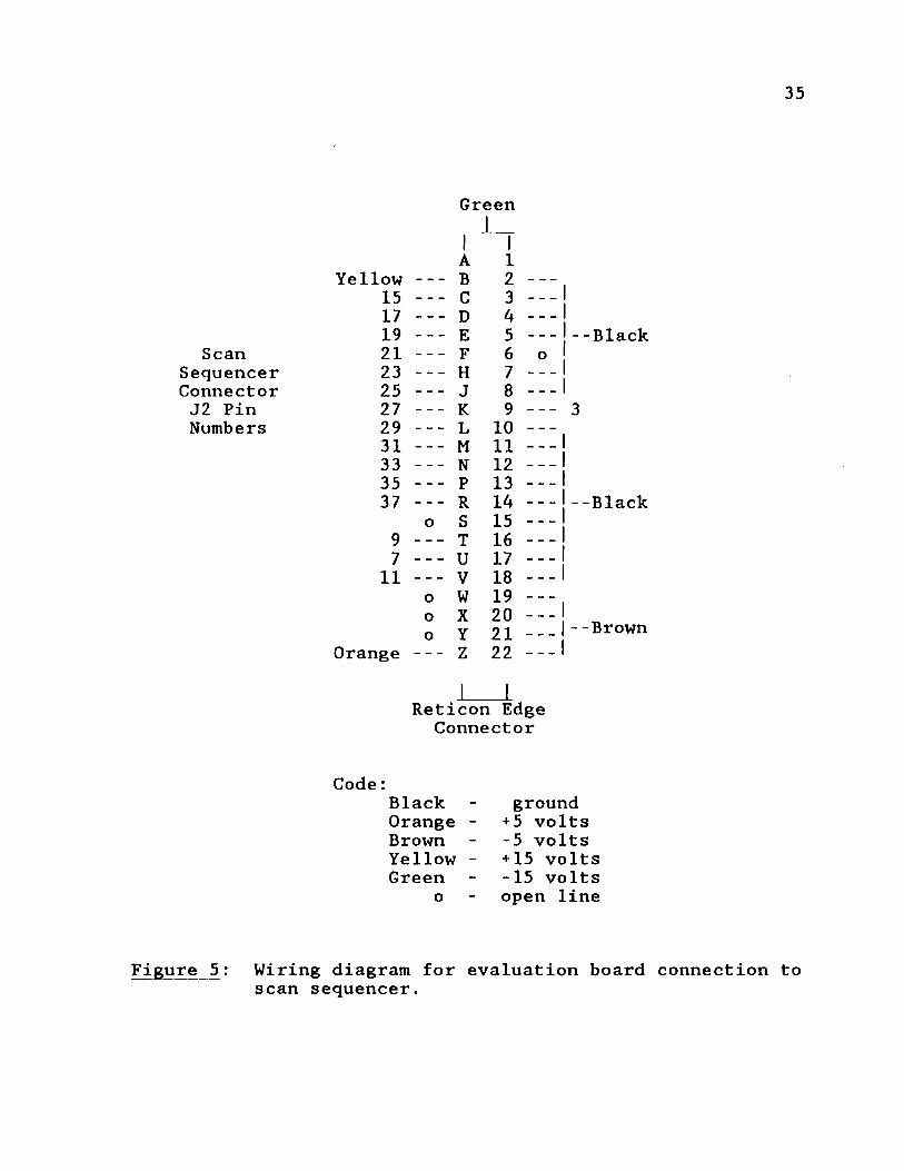
the scan sequencer via a 40 line flat ribbon cable and five power lines ( + /- 5 volts, +/- 15 volts, and ground). Theconnection from the evaluation board output to the edge con­nector is accomplished with wire-wrap. The wiring diagram for this connection is shown in Figure 5. The ribbon cable

connects to pin J2 of the scan sequencer. The circuit dia­

gram of the scan sequencer is shown in Figure 6. In general

this circuit board rectifies timing differences between the

diode array evaluation board's clock and the microcomputer's clock. Table 1 translates the chip designations used.

The scan sequencer is connected to the Tecmar LabMaster board through three coaxial cables and a 16 line flat ribbon

Green

I IA 1

Yellow --- B 2 ---15 --- C 3 ---17 --- D 4 _ _ _

19 --- E 5 ---Scan 21 --- F 6 o

Sequencer 23 --- H 7 ---Connector 25 --- J 8 ---J2 Pin 27 --- K 9 ---Numbers 29 --- L 10 ---

31 --- M 11 ---33 --- N 12 ---35 --- P 13 ---37 --- R 14

o S 15 ---9 --- T 16 ---7 --- U 17 ---

11 --- V 18 ---o W 19 ---o X 20 ---o Y 21 ---

Orange ----- Z 22 ---

- -Black

-Black

Brown

J LReticon Edge Connector

Code:Black Orange - Brown Yellow - Green

o

ground +5 volts -5 volts +15 volts -15 volts open line

Figure 5 : Wiring diagram for evaluation board connescan sequencer.

36

Table 1 : Chips Used for the Diode Array Scan Sequenc­er Board

Designation Chip Type Description

El, E12 Resistors

E2 7404 Hex InvertersE3 7408 Four 2-input positive AND gatesE4 74175 Four D-type flip-flopsa

E5 , E9 74367 Six Bus Drivers, 3-state inputs^E6 7474 Two D-type flip-flopscE7 7402 Four 2-input positive NOR gates

E8, E10 7400 Four 2-input positive NAND gates

Ell 7432 Four 2-input positive OR gates

^Positive edge triggered with double rail inputs. bNon-inverted data outputs, 4- line and 2-line enable inputs.

cPositive edge triggered with preset and clear.

connector. The coaxial lines carry (1) a clock out from the Tecmar, (2) a clock from the scan sequencer to the external start conversion of the Tecmar, and (3) the multiplexed vid­eo signal of the diode array. The video output of the diode array is adjusted to +/-10 volts by the scan sequencer with negative being higher light intensity.

37

£7

£2

to

Ell

ci

• Le

Figure 6: Scan sequencer circuit board design.

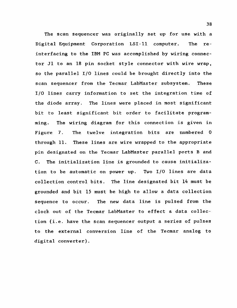
38The scan sequencer was originally set up for use with a

Digital Equipment Corporation LSI-11 computer. The re­

interfacing to the IBM PC was accomplished by wiring connec­tor J1 to an 18 pin socket style connector with wire wrap,

so the parallel I/O lines could be brought directly into the

scan sequencer from the Tecmar LabMaster subsystem. These

I/O lines carry information to set the integration time of the diode array. The lines were placed in most significant bit to least significant bit order to facilitate program­ming. The wiring diagram for this connection is given in Figure 7. The twelve integration bits are numbered 0 through 11. These lines are wire wrapped to the appropriate pin designated on the Tecmar LabMaster parallel ports B and C. The initialization line is grounded to cause initializa­

tion to be automatic on power up. Two I/O lines are data

collection control bits. The line designated bit 14 must be

grounded and bit 15 must be high to allow a data collection

sequence to occur. The new data line is pulsed from the

clock out of the Tecmar LabMaster to effect a data collec­

tion (i.e. have the scan sequencer output a series of pulses to the external conversion line of the Tecmar analog to digital converter).

39Scan Sequencer Connector J1

ground --- A B --- new dataground --- C D --- openground --- E F --- openground --- H J --- 2ground --- K L --- open

14 --- M N --- 15ground --- P R --- openground --- S T --- open

11 --- U V --- openground --- W X --- 10

8 --- Y Z --- 93 --- AA BB --- ground

ground --- CC DD --- 7init --- EE FF --- 6

ground --- HH JJ --- 51 --- KK LL --- 4

open --- MM NN --- groundopen --- PP RR --- open

0 --- SS TT --- openopen --- UU VV --- open

Code:Outer numbers 0-11 are bits to set integration time. Init is the initialization line.Bits 14 and 15 are data collection control bits.Pin B is the new data line.

ground 0i 2i 4i 8i 0i 2i 4i Integration Bits|26 |

11

25124 1

231

22 |1

211

201

19 -| Tecmar Parallel

13 | 121 111 10i 9 1t 81 7i 6 - i Line1

ground11

13

15

17

11 13

15 Integration Bits

Port B | Port C

Figure 7: Wiring diagram for scan sequencer connection toTecmar board.

402.4.4 Software

The program to control the experiment is written in compiled BASIC using assembler subroutines to effect rapid data col­lection. Appendix A is a complete listing of the program CHRAMP6.BAS. This program performs the following functions:

1. Sets the integration time of the diode array.2. Programs the clocks to trigger the laser and scan

sequencer.

3. Initializes the analog to digital converters and calls

the assembler subroutine to collect the data.

4. Retrieves the data from the assembler subroutine and

performs statistical analysis and data reduction.

5. Plots, prints, and/or stores the experimental data.6. In the electrochemical experiments the potential step

is output to the polarograph and the current data is also collected, plotted, and stored in a separate

file.

The program is modularized into subroutines to make it

easier to modify. A new experiment can be run, old experi­mental data can be reviewed, or an old experiment continued

by using different subroutine sequences. The program uses

two screens, one to display the experimental parameters and

another to plot the data as it is collected.

41The integration time of the diode array is set through

the Tecmar LabMaster 8255 parallel port. Digital I/O ports B and C are used. There are 12 bits of control over the integration time. The integration time is dependent on the

scan rate setting of the diode array. Table 2 gives the measured integration times for various settings of the inte­gration switches. To collect this information the integra­tion switches were manually set and the times were read with an oscilloscope. The smallest allowable switch setting is

decimal 34, corresponding to 128 diodes with 4 oscillator clock pulses per sample, plus two additional counts to pro­

vide 8 extra clock cycles to accommodate the settling time

of the DC restoration circuit's switching and charging time

[62]. A setting of 34 at 100 KHz gives an integration time of 1.45 msec. The video signal is 1.3 msec wide for all 128 diodes, regardless of integration time. From the data in

Table 2, a relationship between integration time, switch setting and scan rate can be deduced so the integration time can be selected with software. The decimal switch settings count is the integer value of:

((500-(integration time * scan rate/33333) * 8.19)+1)

where integration time is in mSec and scan rate is in Hz. This gives a number that is the complement of the bit

42pattern that would be set manually. To allow software con­trol the scan sequencer is set with all switches open. A logical NOR is calculated to flip the incoming bits so that the correct switch settings are made. Port B sets bits 0 through 7 and port C sets bits 8 through 11. Bits 12 and 13

of port C are control bits that should be set low for normal

operation. Once the integration time is set, the diode array continually scans at that rate.

Table 2: Diode Array Integration Times

Integration Switch Settingsa Bit Pattern

C : msb B: lsb (decimal)

1111 1111 11 1 (4095)1011 1111 11 1 (3071)0111 1111 11 1 (2047)0011 1111 11 1 (1023)0001 1111 11 1 ( 511)0000 1111 11 1 ( 255)0000 0111 11 1 ( 127)0000 0011 11 1 ( 63)0000 0010 00 0 ( 34)

a0=open, l=closed

Integration Times (msec)

33 KHz 50 KHz 100 KHz

500 333 167375 250 125250 167 83125 83 4262.5 42 2131.2 21 10.515.5 10.4 5.37.8 5.3 2.63.9 2.6 1.45

Timing and event synchronization are very important in an

experiment where several instruments are interfaced together

through the same computer. The Tecmar board has an Am9513

system timing controller that has five 16 bit timer/counters

43[64]. The power and flexibility of these clocks make them very useful in these experiments. Complete clock instruc­tion information can be found in Appendix A, lines 8000-9000. Three of the five clocks are used to control the

experiment. Clock three is the master clock, clock five

controls the pulsing of the laser system, and clock four initiates the scan sequencer.

The diode array is self- scanning, which means that once

the integration time is set, it continually outputs a stream of multiplexed data. This data is only read by the analog-

to-digital converter when the program causes clock four to

pulse, instructing the scan sequencer to output a series of pulses which are channeled to the external start conversion of the Tecmar board. These pulses correspond one-to-one with the positions in time on the multiplexed signal of the diode array's data stream for each diode's output. There are two problems of synchronization. When clock four trig­

gers the scan sequencer, it immediately begins outputting a

series of 128 pulses for the A-to-D converter, corresponding

to the next 128 diode outputs. If the clock four pulse

falls in the middle of the actual scanning of the array (the

1.3 msec window, as opposed to the set integration time) the scan sequencer immediately begins outputting pulses, result­

ing in the 128 data point scan being the end of one read of

the array and the beginning of the next. The laser pulse also must occur during the integration time and not the scan

read time of the diode array. Both of these problems are solved by triggering the scan sequencer to make a dummy reading of 128 diodes, followed by the dual arming of clocks

five and four. Clock five waits 2 mSec to be sure to clear

last array scan, then pulses the laser. Clock four counts a designated time (between 2 msec and the chosen integration

time) then triggers the scan sequencer to cause the array to be read. This sequence is rapidly repeated for a selectable number of times and this series can be averaged.

Clock three is the master clock, which controls the times between the scan series. This can be set up in two ways.

For a repeatable scan series collection rate, the appropri­

ate count down numbers are loaded into the clock and it is

instructed to count repetitively. This series collection

rate should not exceed the time necessary for the software

routines to perform the chosen functions (calculations, printing, plotting, etc.) in between the series. Often in an experiment, the system is changing rapidly at first and

less so with time, so it is desirable to be able to change the series data collection rate as the experiment pro­gresses. To do this clock three is set at the shortest time interval between series collections and a DATA line in the

45program containing a set of numbers is used to instruct the

program which of the series collections are actually to be carried out. For example, if the series read rate is set at 2 seconds and the DATA statement contains 1,2,4,8 the pro­gram will perform a series data collection at times 0 (always), 2, 4, 8 and 16 seconds.

The analog to digital converter is set up by the program to allow repetitive, single channel use with external start

conversions. Channel zero of the Tecmar board is connected to the video output line of the scan sequencer. The BASIC

program calls an assembler subroutine, designated ADC, in

the program SLAVE.ASM to actually perform the data collec­

tions. A listing of this program is given in Appendix B. This subroutine has been stream-lined so that the loop that

does the data collection (LOOP AGAIN) is very efficient. Different command combinations were experimented with and the one that used the least number of clock cycles (i.e. ran the fastest) was chosen [65,66,67],

The subroutine SLAVE.ASM performs the following tasks to effect the rapid data collection:

1. Reserves 130 words of memory for the data.2. Initializes the general registers:

BL with a test pattern for conversion completed (127),

CX with 128, the number of data conversions to per­form ,DX with the port address for the data reading (715H).

3. The data port is then read to reset the done flip flopand interrupts are turned off.

4. AX is used to receive the data value before it ispushed to the stack.

5. The program loop that collects the data performs the

following tasks:a. Checks for conversion done, if not check again.

b. If done read in the data and push it to the

stack for temporary storage.c. Repeat this cycle for a total of 128 data

points.6. The data is then popped off the stack and placed in a

memory location, the first address of which is held in

the variable DATAREA%.7. This variable is passed back to the BASIC program so

that the data can be recovered using memory PEEKS and

is temporarily stored in integer arrays.

There are two problems associated with the use of a

pulsed laser system in these experiments that are handled statistically. There is a pulse to pulse intensity varia­

tion of the laser as well as some spatial fluctuation in the

47cross-sectional shape of the beam. To solve these problems

a series of pulses (usually 10) are collected immediately after one another. The first pulse is generally of signifi­cantly lower intensity than the following ones in a series,

so it is not used. The intensity of the beam is either independently monitored or an area at the far end of the

array (an area not used in the experiment) is used to nor­malize the remaining individual pulses. The normalization is performed by calculating the ratio of the full scale (blank) intensity to the intensity of each experimental pulse. This ratio is multiplied times the intensity reading of each diode in a scan to get the normalized value. Each

of these intensity values is corrected for the dark current

reading before the calculation is made. After normaliza­

tion, a statistical check is run on six diodes of each pulse

(numbers 20, 40, 60, ..., 120) to determine if any of thenine pulses has a significantly different shape than the others. The statistical check consists of calculating the

standard deviation of intensity of the nine pulses at the

six chosen diodes. A user selectable number of standard deviations away from the means of each of the six diodes of the nine pulses constitutes rejecting that pulse. Typically either 2 or 2.5 standard deviations from the mean were used in the experiments, corresponding to 95.5% and 99.7% of the

48observations, respectively [68]. After the series of pulses

are normalized and statistically evaluated, the non-rejected pulses are averaged per diode to arrive at the final value.

This data can then be plotted on the graphics monitor, printed on the screen or hardcopy printer, and/or stored on the computer's hard disk. Information about the experimen­tal set-up is stored in a pseudo-random access file that has

a user input filename and the extension INF. The experimen­

tal data is stored in a separate random access file with the same filename, but with an extension of DAT.

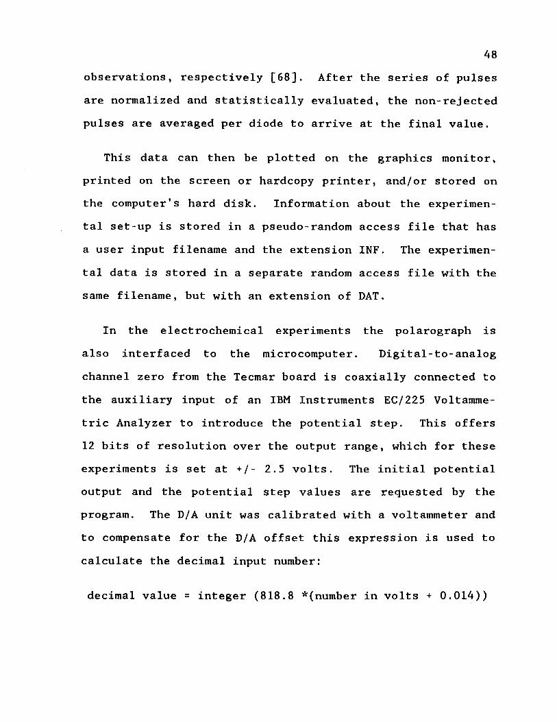
In the electrochemical experiments the polarograph is also interfaced to the microcomputer. Digital-to-analog

channel zero from the Tecmar board is coaxially connected to

the auxiliary input of an IBM Instruments EC/225 Voltamme- tric Analyzer to introduce the potential step. This offers 12 bits of resolution over the output range, which for these experiments is set at +/- 2.5 volts. The initial potential output and the potential step values are requested by the program. The D/A unit was calibrated with a voltammeter and to compensate for the D/A offset this expression is used to

calculate the decimal input number:

decimal value = integer (818.8 *(number in volts + 0.014))

49The current data from the electrochemical cell is also col­lected by the program. Clock three, which counts the maxi­mum spectral data collection rate also causes a software

conversion of channel one of the A/D converter, which is

connected to the recorder output of the polarograph. This data is plotted and stored in a sequential file that is giv­en the extension PRN.

Two other programs are used to further process the spec­troscopic data. The program LOTFIL.BAS, given in Appendix C, can read the data from the compact random access data

file and produce an ASCII file in a format that is compati­

ble with the LOTUS 123 spreadsheet package, for further evaluation of the results. Similarly, the program SASFIL.BAS takes the microcomputer data file and writes an output program that will run under SAS (Statistical Analysis System) on the mainframe computer.

2.5 Preliminary Evaluation of L aser/Photodiode Array

Spectrophotometer

Two simple experiments were carried out to test the lineari­

ty and reproducibility of the laser/photodiode array system. The absorbance of a series of solutions was measured and compared to the absorbance measured with a proprietary spec­

trophotometer. Also the absorbance of a set of four neutral

50density filters (Corion Corp. Holliston, Mass.) of known

optical density were measured. The fixed value, precision neutral density filters have a coating of inconel that attenuates the light by both reflection and absorption.

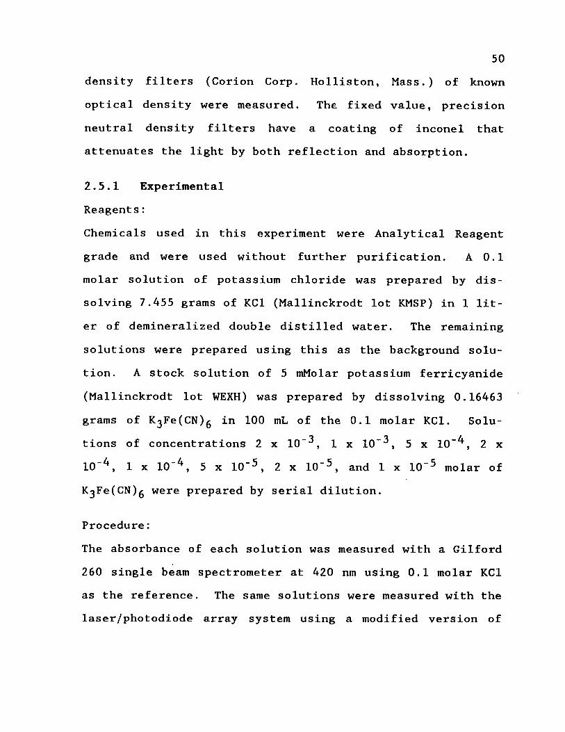
2.5.1 Experimental Reagents:

Chemicals used in this experiment were Analytical Reagent grade and were used without further purification. A 0.1 molar solution of potassium chloride was prepared by dis­solving 7.455 grams of KCl (Mallinckrodt lot KMSP) in 1 lit­

er of demineralized double distilled water. The remaining solutions were prepared using this as the background solu­tion. A stock solution of 5 mMolar potassium ferricyanide

(Mallinckrodt lot WEXH) was prepared by dissolving 0.16463

grams of ^ F e C C N j g in 100 mL of the 0.1 molar KCl. Solu­tions of concentrations 2 x 10"^, 1 x 10"^, 5 x 10~4 , 2 x

10”4 , 1 x 10'4 , 5 x 10"“’, 2 x 10”^, and 1 x 10”^ molar of KgFeCCN)^ were prepared by serial dilution.

Procedure:

The absorbance of each solution was measured with a Gilford 260 single beam spectrometer at 420 nm using 0.1 molar KCl as the reference. The same solutions were measured with the laser/photodiode array system using a modified version of

51the program CHRAMP6.BAS, called LASPEC.BAS. The normaliza­

tion procedure was disabled and the master clock was set so the next series reading could be initiated from the keyboard instead of by software. The laser dye DPS was used to produce light of wavelength 420 nm and a series of twelve pulses were averaged. The full scale measurement was made with 0.1 molar KCl. A standard 1 cm quartz cell was used in all measurements.

The absorbance of the four neutral density filters was

measured using the same program, a wavelength of 400 nm, and an average of nine pulses. The filters were placed before

the beam expander and held at an angle so the reflection would not be back into the dye laser.

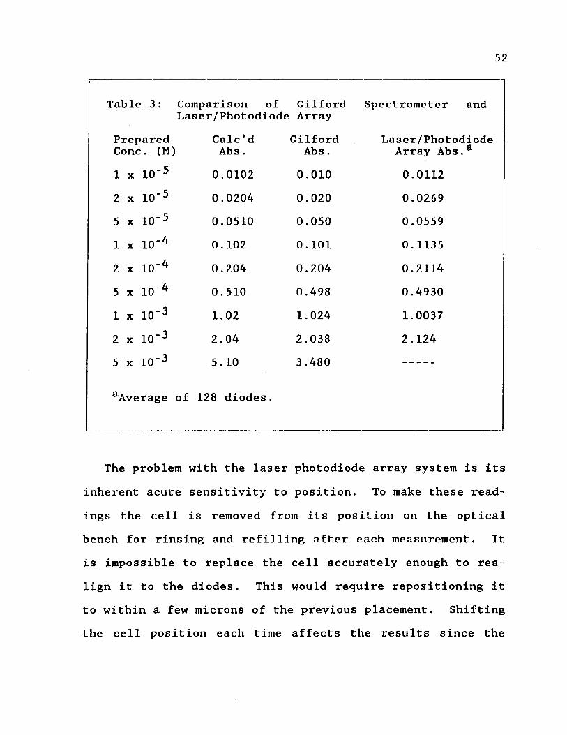
2.5.2 Results and DiscussionTable 3 gives the results of the solution measurements. Plotting concentration vs. absorbance gives a slope of 1019.99 with an intercept of -0.00157 for the data collected with the Gilford spectrometer. Data from the laser/diode

array spectrometer yields a slope of 1051.11 with an inter­

cept of -0.00484. The accepted value for the molar extinc­

tion coefficient of potassium ferricyanide at 420 nm is 1020

(cm-M)"^.

52

Table 3: Comparison of Laser/Photodiode

GilfordArray

Spectrometer and

Prepared Cone. (M)

C alc'd A b s .

Gilford A b s .

Laser/Photodiode Array Abs.a

1 x 10-5 0.0102 0.010 0.01122 x 10-5 0.0204 0.020 0.02695 x 10-5 0.0510 0.050 0.0559

1 x 10'4 0.102 0.101 0.1135

2 x 10-4 0.204 0.204 0.2114

5 x 1(T4 0.510 0.498 0.4930

1 x 10"3 1.02 1.024 1.00372 x 10"3 2.04 2.038 2.1245 x 10"3 5.10 3.480

aAverage of 128 diodes.

The problem with the laser photodiode array system is its

inherent acute sensitivity to position. To make these read­

ings the cell is removed from its position on the optical

bench for rinsing and refilling after each measurement. It

is impossible to replace the cell accurately enough to rea­

lign it to the diodes. This would require repositioning it to within a few microns of the previous placement. Shifting the cell position each time affects the results since the

53calculated absorbance depends on the light path of the full

scale reading, the dark current of the individual diodes, and the new light path for each experimental reading. Con­

sidering this handicap the results are acceptable. This demonstrates the importance of not disturbing the position

of the sample cell in the course of an experiment. Both the spectroelectrochemical and membrane transport experiments

were designed to account for this.

The results for the measurements made with neutral densi­ty filters are given in Table 4. The nature of this meas­

urement differs from the preceding experiment in that there

is nothing comparable to using a blank solution in a cell

for the full scale reading. The full scale reading is just

the intensity of the beam in the absence of the filter of

interest. Therefore positional realignment is not a factor in this measurement. The results show good agreement between the manufacturer's supplied values and the averaged

measured values. The final table entry for the blank is a

measure of the dark current after the experimental readings were made, compared to the dark current before the experi­mental readings were made. This shows the stability of the detector over a period of several minutes while an experi­ment is being conducted. The table entry with two filters was included to demonstrate the additive effect of filters

54used in tandem, since multiple filters were used in most of the following experiments.

From these results a definitive limit of detection is difficult to quantify. Judging from the difference in the diode array measured absorbance and the published absorbance of the neutral density filters, an estimated accuracy of

(+/-) 0.02 absorbance units is a conservative estimate.

Table 4: Absorbance of Fixed Filters

Value Neutral Density

Filter(s) Reported Optical Density

Averaged Measured Optical Density®

QD-10 0.086 0.084

QD-30 0.273 0.250

QD-50 0.456 0.453QD-100 1.00 0.98

QD-100,QD-30 1.27 1.26QD-200 2.00 2.01

Blank --- 0.002

aAverage of 128 diodes.

552.5.3 SummaryBased on these preliminary experiments the laser/photodiode array system should function adequately as a simple spec­

trometer. The next chapter describes experiments to show

that it also can function as a positionally resolved spec­trometer .

Chapter III APPLICATION TO AN ELECTROCHEMICAL SYSTEM

3.1 Theory

The formation of an electrochemical diffusion layer was cho­sen for the first study because it is a well-defined system.

When certain conditions are met, a concentration distance

profile develops in the solution above an electrode as a function of time that is theoretically predictable. The

reliability of the spectroelectrochemical system can be ver­

ified by electrochemical measurements, independent of the optical measurements. Thereby, the performance of the laser/photodiode array spectrophotometer can be tested for accuracy in a known system.

3.1.1 ChronoamperometryThe electrochemical technique used in these experiments is chronoamperometry. This technique involves forcing a simple potential step from the electro-inactive region to the electro-active region of a redox system in an electrochemi­

cal cell and measuring the current that flows between the electrode and solution as a function of time. If three

- 56 -

57conditions are met, this current is given by the Cottrell equation:1. Before the potential is stepped, the solution must be

homogeneous.2. Mass transfer to the electrode is restricted to semi­

infinite linear diffusion which means that there can

be no mechanical or thermal convection, and no migra­tion due to an electrical gradient. In addition the

formation of the diffusion layer cannot be obstructed,

that is, there should always be some position above the electrode where has the solution still has the

original bulk concentration.

3. The potential must be stepped high enough that the surface concentration of the species is essentially zero. This just means that the rate of the reaction is mass transfer controlled. The limiting factor is diffusion to the electrode and not the kinetics of the reaction at the electrode surface.

When these conditions are met the current as a function

of time, i(t), is given by:

1/2 * nFAD0/ CDi(t) = — --- eq.3-1

( t )

58which is the Cottrell equation, where DQ is the diffusion coefficient and CQ is the bulk concentration of the reacting

species 0, t is time, n is the number of electrons trans­ferred per mole of reactant, F is the Faraday constant, and A is the electrode surface area [69,70]. From equation 3-1

it can be seen that at the onset of the potential step the current will be the highest (t --> 0) since the concentra­tion of the reacting species is highest at the electrode surface at this time. The current progressively decays since the surface concentration of the reactant decreases as a function of time.

3.1.2 Concentration as a Function of Position and Time When mass transport is limited to diffusion, concentration

change as a function of time and distance is characterized by Fick's second law, which states:

dC (x,t) _ d2C (x,t) 2--------- “ D0 (-----^-5-----) eq.3-2

dt dx

where CQ (x,t) is concentration of the reacting species, 0, at position x and at time t. This is a second order, linear partial differential equation that can be solved by imposing the boundary conditions of the Cottrell equation for chro­noamperometry at a planar electrode and using the Laplace transform [71]. The result is:

59

C0 (x,t) - c” erf(-------- TT5- ) eq.3-32(D0t)1/2

where erf(z) is the error function integral of z. In this

case, x is the distance from the planar electrode surface and t is the time after the potential is stepped.

To get the concentration profile of the product of the electrode reaction, Cp(x,t), Fick’s second Law is again used:

dC (x,t) _ d2C (x,t)P - D (-----P— -----) e q . 3-2adt P dx2

where Dp is the diffusion coefficient of the product. The following boundary conditions exist in this case:

1. At time zero the concentration of product is zero throughout the cell.

2. After the potential step, there is a position above the electrode surface where the concentration of prod­uct is still zero.

3. The formation of product at the electrode surface, Cp(x=0), is equal to the disappearance of reactant:

dC (x=0) dC (x=0)DP ^ -----) ■ -” o <-----

60Applying these conditions to the product concentration and the previous conditions to the reactant and again using the Laplace transform, the following equation can be derived for

the concentration profile of the product of a chronoampero- metric reaction at a planar electrode:

D 0 i / o >v ^cp (x>t) = (“n- > co I1 - er£(-------- T r T >1 eq-3-5DP 2(Dp t ) /

Complete derivations of the concentration profile equations can be found in reference [70].

An exact solution to the error function integral is not obtainable. It can be closely approximated however, with two different calculations using series. For values of z from zero through two, the Maclaurin expansion that does this is:

2 z3 z5 z7erf(2) = ^ r r (z • 5 n T * w i - w T * •••> e q -3-6

where z is the expression enclosed in parentheses in the

error functions of equations 3-3 and 3-5. For values of z greater than two, the expression:

2rz X 1 e "z /I 1 1*3 1*3*5 . , ,erf(z) = 1 --- — — ( 1 ---- + — -------- — - +...) eq.3-7

tt z 2z2 (2z ) (2z )

better approximates the error function integral [69].

61Equations 3-3 and 3-5 were used in combination with equa­

tions 3-6 and 3-7 to calculate theoretical concentration/

distance/time profiles of the reactant and product respec­tively for comparison to experimentally obtained profiles.

The compiled BASIC program CONCPRFL.BAS uses these expres­sions to calculate, plot, and store the relative concentra­

tion values over a given distance with 25 micron resolution at specified times and diffusion coefficients. A listing of this program is given in Appendix E.

In general the two diffusion coefficients are quite close to one another, so the term (D0 /Dp ) in equation 3-5 is close to one. When they are equal the two concentration profiles

are symmetrical. This case is shown in Figure 8. Relative concentration is the concentration of the reactant or prod­

uct expressed as a fraction of the bulk concentration ofV' tVreactant, (C0 (x,t)/CQ ) and (Cp (x,t )/CQ ), respectively. When

the diffusion coefficient of the product of the electrode reaction is greater than that of the reactant, the relative

concentration at the surface of the electrode is less than 1 and is given by the square root of the ratio of the diffu­

sion coefficient of the reactant to that of the product.This is shown in Figure 9 for a case where the reactant dif-

ft 9fusion coefficient is 5 x 10 cm /sec and the product diffu--ft 9sion coefficient is 6 x 10 cm /sec. Likewise if the

62diffusion coefficient of the product is less than the reac­tant the relative surface concentration is more than 1 as shown in Figure 10.

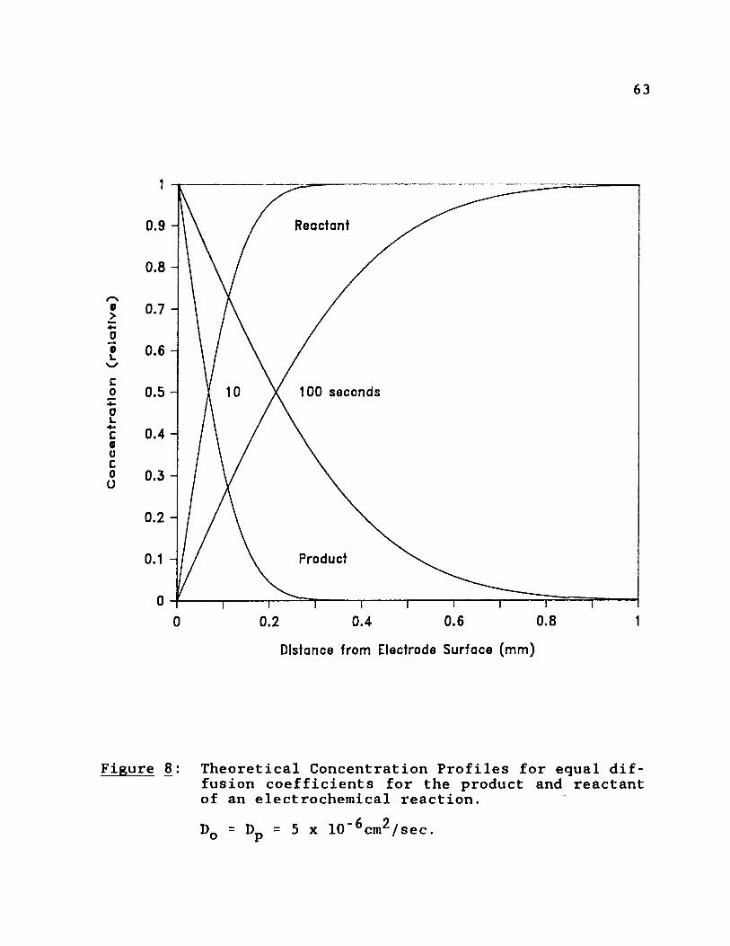
Co

ncen

trati

on

(r

ela

tiv

e)

63

Reactant0.9 -

0.8 -

0.7 -

0.6 -

100 seconds0.5 -

0.4 -

0.3 -

0.2 -

Product

0.6 0.80.40.20Distance from Electrode Surface (m m )

Figure 8: Theoretical Concentration Profiles for equal dif­fusion coefficients for the product and reactant of an electrochemical reaction.

DQ = Dp = 5 x 10”^cm^/sec.

Co

ncen

trati

on

(r

ela

tiv

e)

64

0.9 Reactant

0.8 -

0.7 -

0.6 -

0.5 - 100 seconds

0.4 -

0.3 -

0.2 -

Product

0.80.60 0.2 0.4Distance from Electrode Surface (m m )

Figure 9: Theoretical Concentration Profiles for unequaldiffusion coefficients of the product and reac­tant of an electrochemical reaction.DQ = 5 x 10"^cm^/s; Dp = 6 x 10"^cm^/s.

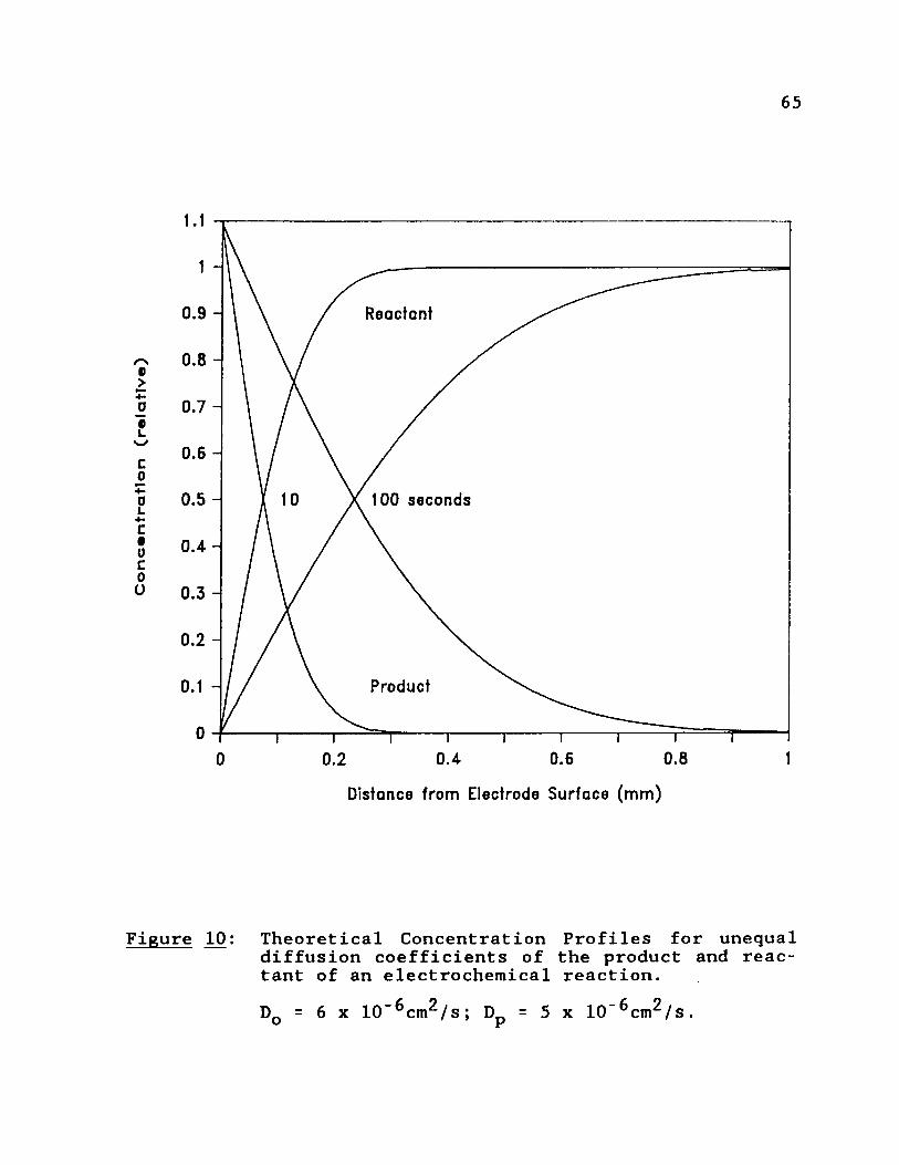
Co

ncen

trati

on

(r

ela

tiv

e)

65

0.9 - Reactant

0.8 -

0.7 -

0.6 -

0.5 - 100 seconds

0.4 -

0.3 -

0.2 -

Product

0.80.4 0.60 0.2Distance from Electrode Surface (m m )

Figure 10: Theoretical Concentration Profiles for unequaldiffusion coefficients of the product and reac­tant of an electrochemical reaction.DQ = 6 x 10”^cm^/s; Dp = 5 x 10“^cm^/s.

663.2 Spectroelectrochemical Cell A ssemblyIn order to meet the boundary conditions set down by the experiment, the spectroelectrochemical cell must fulfill several requirements:

1. The surface of the indicator electrode must be very

flat and smooth in order meet the Cottrell conditions

and to be able to observe events close to its surface.2. The walls of the cell must be perpendicular to the

indicator electrode surface so that diffusion can only be linear.

3. Two opposing walls must be flat and optically trans­parent down to the electrode surface to make a useful spectroscopic reading.

4. The cell must be water tight to maintain quiet solu­tion conditions.

5. Access must be allowed to the solution in the cell for

contact to the reference and auxiliary electrodes.

Designing and constructing a cell that meets these

requirements proved to be a challenge. Several different

electrochemical cell designs were experimented with.

Attempts to build the cell out of two separate glass windows

and the electrode held together with aluminum or plastic mountings, invariably resulted in leaking. The idea of carefully carving the indicator electrode so it would fit

67into a piece of square-bore glass tubing was also tried.

With wax sealant, leaking was not a problem, however the cell was very delicate and susceptible to breakage. Almost any stress against the indicator electrode, which is neces­

sary to maintain electrical contact, caused the glass cell

to crack.

The cell that worked best is shown in Figure 11. In this cell a piece of square-bore glass tubing whose cross-section is polished to a high degree of smoothness serves as the cell walls. This is tension mounted against a similarly polished graphite electrode without a washer or sealant. If

the two pieces are carefully polished to be both smooth and

flatly perpendicular to their lengths, the cell is water tight. The square-bore glass tubing has inside dimensions

of 2 mm by 4 mm ( + /-0.2 mm). This was specifically chosen

so the conversion to a membrane transport study could be done more easily and under comparable optical conditions.

In order to be able to use the spectroelectrochemical

results to validate the membrane transport results, the optical conditions of the two experiments should be as near­ly identical as possible.

Graphite electrodes have been used in voltammetry since their introduction by Gaylor et a l . in 1953 [72,73]. It

68continues to be a popular choice of electrode material for detecting organic compounds [74].

69

Figure 11: The assembled spectroelectrochemical cell

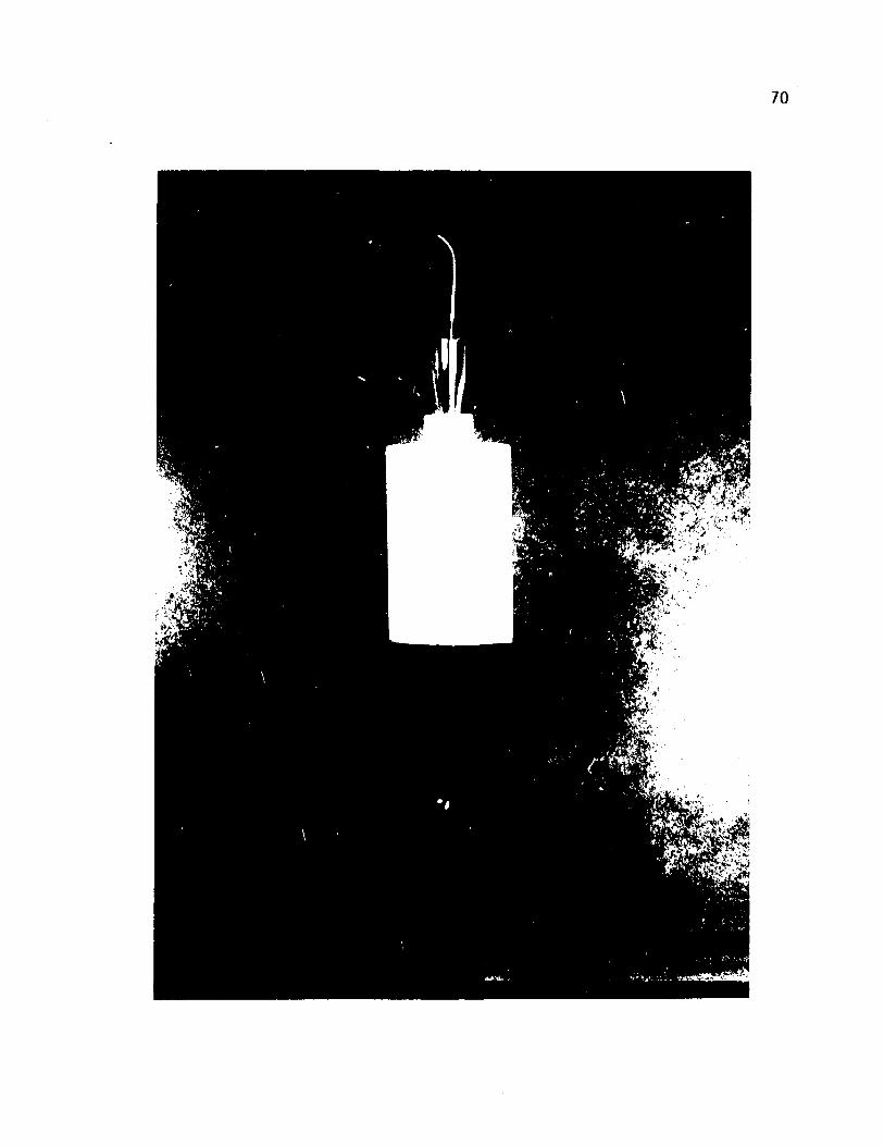
713.2.1 Glass Cell Preparation:

The following procedure was developed to prepare the square- bore glass tubing. All polishing compounds, lubricants, paper disks, and cloths were purchased from Buelher Ltd. (Lake Bluff, 111.). Mechanical polishing was performed on a

Buelher 69-1000 Minimet (R) Polisher/Grinder. High quality rectangular bore tubing, 2 mm by 4 mm inner dimensions, 0.7 mm wall thickness, made of borosilicate glass was obtained

from Wilmad Glass Co. (Buena, N.J., Catalog number WR-0204).The exact inside dimensions of the rectangular bore glasswere measured with a caliper because of variability from

piece to piece. This is important to know for the spectro­scopic calculation.

1. Glass Preparation: A glass cutting wheel was used toget three 2.2 cm pieces of the square bore tubing with

the cut as flat and as perpendicular to the length aspossible and free of chips on the edges. These are secured in Teflon holders which are made by drilling 5 cm sections of half inch diameter Teflon rod about 3

cm deep such that the pieces fit snugly. The first cm of these Teflon holders are threaded 7/16 x 20 to fit

in a one-half inch thick, 3 inch diameter Kel-F disk

that has been tapped symmetrically with three holes

and threaded to accept the Teflon pieces. The Kel-F

disc has a small depression drilled about one- sixteenth of an inch deep in its center for contact with the load arm of the polisher. When mounted in

the holder, the three pieces of glass should protrude about 2 mm below the holder. The Teflon rods can be

screwed into the Kel-F disk so that the glass pieces stick out an even distance from it. This technique securely holds the square-bore glass and evenly

applies pressure to the three pieces so the polishing will be perpendicular to their length and uniform over their surfaces.

Fine Grinding: In the holder the three pieces areground by hand with 240 grit and then 300 grit Carbi- met (R) paper discs for about 2 minutes each. The pieces are then polished on 400 grit Carbimet on the

Minimet Polisher lubricated with a few drops of lap­

ping oil, until the surfaces are no longer opaque, but

still may exhibit visible scratches. The load adjust­

ment should be set manually so the load arm firmly

holds the sample against the abrasive paper. The holder should move smoothly over the paper surface.

If not, more lubricant may be needed or the load ten­sion may be too high.

Rough Polishing: In general finer and finer diamondpolishing compound is used to achieve a very flat, smooth surface. The glass surface will be free of any

visible scratches or grooves. Inspect the glass sur­face after each size of diamond compound is used. If

scratches do not systematically disappear, repeat that phase or go back a size or two until improvement is noted.

Abrasives: 45u, 15u, 6u, lu, l/4u Metadi(R) diamondcompound.

Cloth: Texmet(R) polishing cloth.

Lubricant: Automet(R) lapping oil (3-4 drops).

Procedure: Use speed 2 for about 8 minutes (setting 9

twice) then speed four for about 8 minutes for each of the abrasives.

Fine Polishing: The glass should be very smoothbefore fine polishing is attempted. This step puts a

glossy finish on the glass surface but will not remove

any significant scratches. If scratches still exist repeat some of the rough polishing. When this step is properly completed the glass surface has a flat melted appearance.Abrasives: Alpha 1C alumina A (lu), Alpha 2 alumina C (.3 u ), and Gamma 3 alumina B (.05u) Micropolish (R).

Cloth: Microcloth (R) polishing cloth.

74Lubricant: Double distilled water.

Procedure: Use speed two for 11 minutes (setting 9 times 3), then speed four for 8 minutes for each size of alumina. The load should be snug.

3.2.2 Indicator Electrode Preparation:

Fine grain, low permeability graphite (DFP-1 Grade, POCO Graphite Inc., Garland, Texas) was specially prepared to use

as the indicator electrode. A 5/8 inch graphite rod was machined to 6 mm diameter and cut to 14 mm lengths. This

Ohas an average density of 1.79 gm/cm and an average pore size of 0.4 microns.

1. Graphite Preparation: To avoid solution permeationand "electrode memory" problems, the graphite was

impregnated with Nujol (mineral oil) [73,75]. The machined piece of graphite is washed thoroughly in

hexane and dried in an oven at about 70°C for thirty minutes. While still hot, this is placed in mineral oil (Medi-Kay Laboratories, Brookfield, Mo.) and

placed under vacuum (about 0.1 mm Hg) for about five

hours (or overnight). The carbon piece is rinsed with

distilled water and polished according to the follow­

ing procedure.

2. Fine Grinding: A holder identical to the one

described for the glass preparation was used except

the Teflon holders were drilled to 6 mm inner diameter

and were tapped on the side to allow a brass screw to hold the graphite piece securely in place. Graphite is softer than borosilicate glass, so in general it

requires less harsh treatment. The graphite pieces are ground on a 600 grit Carbimet (R) paper disk with 3-4 drops of lapping oil just until they are uniformly

flat. This will take about one minute, depending on how smooth the pieces were made. The tension is adjusted to get a firm hold. Grinding is relatively fast with graphite, so the pieces should be checked

often.Rough Polishing: Finer and finer diamond compound isused to systematically remove scratches. Significant scratches should be completely gone after this phase.

If not repeat all or part of it. Rinse thoroughly

between abrasives with distilled water and dry by

blotting with a paper tissue.

Abrasives: 15u, 6u, lu, l/4u Metadi(R) diamond com­

pound .

Cloth: Nylon polishing cloth.Lubricant: Automet (R) lapping oil (3-4 drops). Procedure: Use speed 2 for about 4 minutes (setting 9) then speed four for about 4 minutes for each abrasive.

764. Fine Polishing: This phase gives a shiny finish to

the graphite. Because of the graphite particle size, a glassy finish will not be achieved. Instead the

surface begins to sparkle in bright light as a better

finish develops. Repeat this step if necessary, to get this kind of finish.Abrasives: Alpha 1C alumina A (lu), Alpha 2 alumina C (.3u), and Gamma 3 alumina B (.05u) Micropolish (R). Cloth: Microcloth (R) polishing cloth.Lubricant: Double distilled water.Procedure: Use speed two for 8 minutes (setting 9

times 2), then speed four for 4 minutes for each abra­

sive. The load should be snug.

3.2.3 Reference and Auxiliary Electrode Preparation:

A silver wire coated with a layer of silver chloride serves as the reference electrode. This is prepared as follows:

1. Approximately 10 cm of 20 gauge silver wire is washedwith soapy water, rinsed well, and scraped with a razor blade to expose a fresh surface.

2. About half of this is immersed in a 0.1 N HCl solutionand connected to the positive terminal of a 1.5 volt

battery with regular wire.3. A short piece of platinum wire immersed in the solu­

tion completes the circuit. This is held inside a

77section of 8 mm glass tubing with a fritted glass enclosure at the end to direct the hydrogen gas formed at this electrode out of the solution.

4. The silver chloride appears as a mossy gray coating on the immersed portion of the silver wire. This is allowed to develop for about 1.5 hours. The electrode

is allowed to air dry and set overnight before use.

The Ag/AgCl electrode has standard potential of +0.2224 volts at 25°C [76]. It is sturdy and chemically inert to the compounds used in this study and also does not require a

salt bridge. The electrochemical potentials reported are in

reference to the Ag/AgCl electrode. The Ag/AgCl electrode is enclosed in glass capillary tube or a shortened disposa­ble Pasteur pipet. A 31 gauge platinum wire wrapped around the glass encased Ag/AgCl serves as the auxiliary electrode.

3.2.4 Spectroelectrochemical Cell Holder:The assembly that holds the two main parts of the spectroe­

lectrochemical cell together, the graphite electrode and the

rectangular bore glass, should be opaque to decrease stray

light reaching the detector and have an open light path at

and just above the electrode surface. The two pieces must

be held together firmly and perpendicularly without horizon­

tal stress. Three plastic pieces were specially made to fit together to do this.

The graphite electrode is held in a 0.5 inch diameter

polycarbonate cylinder, drilled 0.55 inch deep at one

end with a 0.25 inch drill bit. About the first 0.3inches of the same end is threaded 7/16 x 20 on the

outside. Just beyond that, about 0.4 inches from theend, a hole is made through to the opening on theinside of the cylinder and is threaded to 2-56. A 0.5

inch 2-56 brass screw, filed to a point at the end, is

used to hold the graphite rod in place and to maintain electrical contact with the electrode.A 1 cm diameter Teflon rod, about 5.5 cm long is drilled through its length with a 0.4 cm hole. One end is further drilled to 0.5 cm diameter, 0.7 cm deep. The rectangular bore glass piece fits loosely

in this end and protrudes about 1.4 cm. Teflon is

used here because it will give some when pressure is

applied to it.

A 2.75 inch rod of 1 inch diameter nylon is modified to hold the other two pieces together. It is drilled

through its length 0.4 inches to form a cylinder. One end is tapped on the inside 7/16-20 to receive the polycarbonate electrode holder. At 0.4 inches from the tapped end a 0.3 inch hole is drilled through the center of the cylinder perpendicular to its length to

79serve as the light path. About 1.9 inches from the tapped end of the cylinder a hole is drilled parallel

to the light path hole through to the center opening only and is tapped 6-32. A 1 cm nylon screw is used here to hold the glass cell containing Teflon cylinder in place. In order to be able the get the cell as close to the detector as possible, the back of the nylon cylinder is machined flat. About 0.15 inch was removed over the entire length and another 0.1 inch depression (0.7 by 1 inch) was removed directly behind

the light path opening. The diode array chip (IC)

fits into the concave recession, effective blocking stray light. The bottom 1.5 inches of the nylon piece

is painted matte black inside and out to decrease stray light penetration even more.

The spectroelectrochemical cell is assembled by first mounting the graphite electrode in the polycarbonate rod, securing it in place with the brass screw. The graphite should protrude at least 1 mm above the rod and may require some adjustment to get the surface perpendicular. The poly­carbonate holder with the electrode is then screwed into the

bottom of the nylon holder. This is inverted and the Teflon piece with the rectangular bore glass tube loosely placed in it, is slipped through the nylon holder until the two

80polished surfaces squarely meet. This is held down firmly while the nylon screw is tightened onto the Teflon cylinder to maintain the vertical tension. The glass piece fits loosely in the Teflon cylinder so this can be tightened without putting torque or horizontal pressure on i t . A dis­

posable Pasteur pipette can be used to introduce solution into the cell from the top through the Teflon piece. Also,

the silver/silver chloride reference electrode and platinum auxiliary electrode make contact with the solution through this opening. A picture of the assembled and disassembled

cells can be seen in Figure 11 and Figure 12.

81

F igure 12: The disassembled spectroelectrochemical cell.

8 2

833.3 ReagentsAnalytical Reagent grade chemicals were used in this section without further purification. Background solutions of 0.2 molar KC1 (Mallinckrodt lot KMSP) with 0.02 molar HCl (Fish­er lot 735224), 0.1 molar KCl with 0.01 molar HCl, and 0.1

molar KCl with 0.1 molar HCl were prepared with demineral­ized double distilled water.

Solutions of 1.0 mMolar and 0.1 mMolar K ^ F e ^ N ) ^ were prepared by serial dilution from 10 mMolar ^ F e ^ N ) ^ (Mal­linckrodt lot WEXH) in the 0.1 M KCl/0.01 M HCl background

solution. These solutions were tested spectrometrically for

composition. Solutions of 4.0 mMolar, 1.0 mMolar, and 0.1 mMolar K^Fe(CN)^ were prepared by serial dilution from 10.0 mMolar K^Fe(CN)g (Baker lot 33407) stock solution in 0.2 M KCl/0.02 M HCl. Potassium ferrocyanide is light sensitive and is easily air oxidized. These solutions were purged of dissolved oxygen by bubbling (Zn/vanadyl sulfate scrubbed)

nitrogen gas through them for about 15 minutes [77], The

ferrocyanide solutions were prepared and stored in volumet­

ric flasks painted black to keep the light out. These solu­

tions should remain clear. Fresh solutions were prepared daily from stock solution.

84A solution of 10 mMolar o-tolidine was prepared by dis­

solving 0.32123 grams of o-tolidine.2HCl.2H 2O (Sigma lot

63F-0410) in 0.1M KC1/0.1M HCl. Solutions of 1.0 mM and 0.1 mM o-tolidine were prepared by serial dilution. These solu­tions are assayed spectrophotometrically at 282 nm where o-tolidine has a molar extinction coefficient of 29,000

( c m - M ) F r e s h solutions were prepared daily from stock solution.

3_.4 Evaluation of the Electrochemical CellThree simple experiments were conducted to characterize the spectroelectrochemical cell for voltammetric performance. To test for a tight seal between the glass walls and the

electrode without a thin layer electrochemical effect, cycl­

ic voltammograms were collected. Adherence to Cottrell con­

ditions were checked with chronoamperometric measurements.

A series of linear sweep voltammograms were collected at various sweep rates to ensure mass transport to the elec­

trode surface is limited to linear diffusion.

3.4.1 Experimental Procedure

All electrochemistry was performed with an IBM EC/225 Vol­tammetric Analyzer. This was interfaced to the microcom­puter, as described previously, to perform the potential step and collect the data for the chronoamperometric

85measurements. It was used with an X-Y recorder for the lin­ear sweep and cyclic voltammetry measurements.

The electrode surface is renewed regularly by rinsing

with demineralized double distilled water followed by gentle rubbing on a tissue. Every couple of weeks the surface smoothness was re-established by repeating the final fine polishing procedure (see section 3.2.2). The spectroelec­trochemical cell is assembled and filled with approximately

100 uLiters of the test solution of interest. The

reference/auxiliary electrode assembly is thoroughly rinsed

with demineralized double distilled water followed by rins­

ing with the test solution. It is placed into the cell solution, leaving a 4-5 millimeter gap between the tip of

the reference electrode and the indicator electrode surface. With use, the reference electrode discolors, so the silver

chloride coating is periodically replaced.

Cyclic voltammetry involves applying a triangular wave­form to an electrochemical cell and measuring the current as a function of potential. In this experiment a scan speed setting of 15 millivolts/sec was used. This was calibrated with an oscilloscope and found to be 14.92 mV/sec. The

results were collected on an X-Y plotter. Typically a cyclic voltammogram of the background solution would be

86collected first, the solution of interest would then be measured one or more times, and the background solution would be measured again. The cell was thoroughly rinsed between measurements with demineralized double distilled water followed by rinsing with the solution to be measured.

Linear sweep voltammetry involves applying a potential

ramp to an electrochemical cell and measuring current as a function of potential. Linear sweep voltammograms were col­lected using sweep rates of 5.08, 9.98, 18.85, 39.04, 49.28. and 86.96 mV/sec (calibrated values).

Chronoamperometry has been discussed in section 3.1.1. These chronoamperograms were collected with a program that outputs the chosen potential step and collects the current data from the Y terminal of the X-Y recorder. A listing of the program CA.BAS is provided as Appendix F. The program plots, stores, and/or extracts surface area or diffusion

coefficient information from the current data.

3.4.2 Results and Discussion

A representative cyclic voltammogram is shown in Figure 13.

The theory behind cyclic voltammetry and linear sweep vol­tammetry was developed by Nicholson and Shain [78]. The interest here is limited to the evaluation of the peak cur­

rent, ip. The equation relating peak current to the experi­mental parameters is:

87ip = (2.69 x 105 ) eq.3-8

where v is the potential sweep rate and the other terms are as defined in equation 3-1. This is commonly known as the

Randles-Sevcik equation after the two men who first reported it in 1948 [79]. The requirements for adherence to this

equation are basically the same as the Cottrell conditions.

A thin layer in an electrochemical cell displays a charac­teristic sharp peak on the voltammetric wave that does not follow equation 3-8. The absence of this peak indicates a good seal between the glass walls and graphite electrode without a thin layer effect.

The cyclic voltammogram of Figure 13 yields three inter­esting pieces of information.

1. From equation 3-8 the electrode surface area can be

calculated. The diffusion coefficient for K^Fe(CN)gO

is 6.5 x 10-Dcm^/sec [80]. The calculated electrodeOsurface area is 0.0776 cm . The measured or geometric

surface area, as defined by the inside dimensions ofpthe rectangular bore glass, is 0.0770 cm (0.195 cm by

0.395 cm), which is good agreement. This indicates

that the electrode polishing procedure produced a very smooth surface.

88

.8

.4

<*

0c*>i.•»oU

.4

.8

3 0.4 2.5Volts

Balanced equation of the K^FeCCNjg/K^FeCCN)^ redox reaction:

K 4Fe(CN)6 = K 3Fe(CN)6 + K + + e"

Figure 13: Cyclic Voltammogram of K^Fe(CN)g

892. The ratio of the forward to the reverse peak current

should be 1 for a nernstian system. As can be seen both i_ _ and i_ _ are 6.5 u Amps, so this holds true.r » d r i

3. A good criterion of electrode process reversibility is

the difference in the peak potentials for the anodic, E_ _, and cathodic, E„ waves. For an ideallyP y Cl F i L

reversible redox system:

0-058Epa " Epc = Volts eq.3-9

In this case n is 1 and the measured E_ _ - E_. a is 60P j C P i d

mVolts, indicating a reversible system.

Figure 14-a shows a series of six linear sweep voltammo- grams for the reduction of K^FeCCN)^. From equation 3-8 it can be seen that peak current in these wave should be pro­portional to the square root of the sweep rate, v. This is

a good criterion for linear diffusion to the electrode sur­

face. Figure 14-b is a plot of the square root of the scan

rate vs. ip/((2.69x10^ )Dq /^C*). The number of electrons

transferred per mole of reactant, n, is 1 for KgFeCCN)^. The slope of this plot is the apparent or effective elec-

Otrode surface area, 0.080 cm . Except for the fastest sweep rate the linearity is good, which could be due to a poor

recorder response time. The last value was excluded from

90the slope calculation. Table 5 gives these results plus the calculated electrode surface area for each scan. The peak

current is measured from a baseline that is a continuation of the initial flat part of each scan to account for back­ground and charging current [80]. The apparent electrode

surface area is fairly close to the geometric determinedOvalue of 0.0770 cm for this piece. The linearity of this

plot indicates that mass transfer to the electrode surface is limited to linear diffusion.

Table 5: Apparent Electrode Surface Area at VariousScan Rates Using Linear Sweep Voltammetry

Scan Rate Peak Current Electrode Surface

(V/sec) (uAmps) pArea (cm )0.00508 4.00 0.0755

0.00998 5.75 0.07740.01885 7.50 0.07350.03904 11.5 0.07830.04928 13.0 0.07880.08696 22.5 0.1027a

aExcluded by Q test.

91

Figure 14: Linear Sweep Voltammograms of K 3Fe(CN)6 and plotof i v s . X

where X= ip /((2.69xl05 )d J/2C* ) .

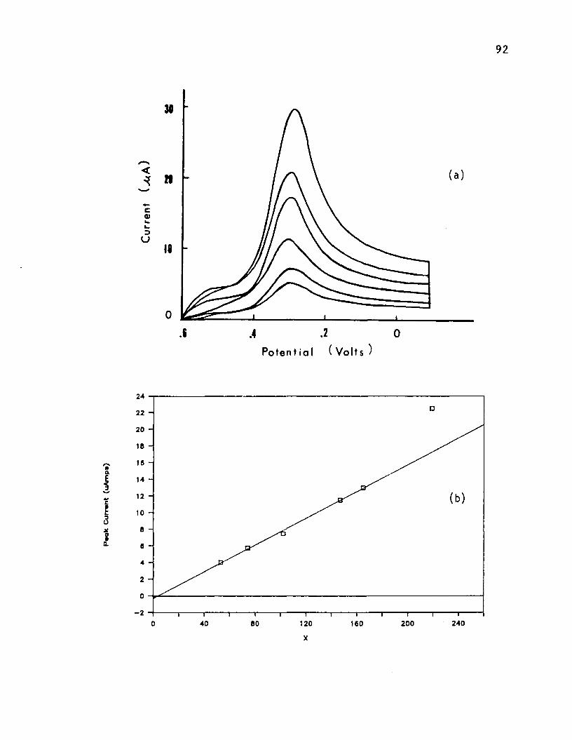
Paok

C

urra

nt

(uA

mp

a)

92

c0)k»k .3u

30

N

10

0.2S .4 0

Potent ia I ( Volts )

24

2220

-224020040 80 120 1600

X

93Probably the best overall gauge of electrode performance

as a function of time is chronoamperometry. Figure 15 shows a chronoamperogram and a plot of apparent electrode surface area as a function of time for 1.0 mM potassium fer-

rocyanide. Electrode surface area is, of course, a con­stant. This second plot is an indicator of cell conditions

as a function of time. The current, and therefore the apparent electrode surface area, will not follow theory if cell conditions are not constant. Most often the discrepan­cy is due to convection within the cell solution. Convec­tion can arise from room vibrations or density gradient for­

mation. Density gradients are a problem if the product of the electrochemical reaction is lighter than the reactant in

a cell set up for downward diffusion, such as this one. The

product, ferricyanide, is lighter than ferrocyanide so it tends to convectively move up from the electrode where it is formed, stirring the solution and resulting in deviation

from Cottrell conditions. This becomes a problem only after several minutes of reaction, however [81,82].

In this case the agreement with theory is quite good. Theoretical current is depicted as crosses in Figure 15. The average electrode surface area from Figure 15 is 0.0718

Ocm . The measured area as defined by the rectangular glass is 0.070 cm^ (0.182 cm by 0.385 cm) for this piece. It

94appears from these graphs that the Cottrell conditions are maintained for at least 120 seconds. This data was actually collected during a spectroelectrochemical experiment at a data point every 2 seconds.

One other electrochemical measurement was made. The dif­fusion coefficient of o-tolidine must be known to make the

theoretical calculation in the spectroelectrochemical meas­

urements. This has been reported to be from 3.8 x10~^cm^/sec [83] to 6.5 x 10~^cm^/sec [84]. Using the elec­

trode surface area value obtained with the K^Fe(CN)g chro-- 5 ?noamperograms, a diffusion coefficient of 5.72 x 10 cm /sec

is calculated from the Cottrell equation using chronoampero- metry with the cell described.

95

Figure 15: (a) Chronoamperogram of K^Fe(CN)g (b) Plot ofApparent Electrode Surface Area as a Function of T i m e .

96

S.?Eujooc»m •UO '—

1(a )

Thaoratloal

4 -

0 40 60 eo 100 12020T im a ( j i o o n d a )

CM:EoaaL.<Oor3VI•TJ£O

c2oaa.<

0.15

(b)0.14 -

0.13 -

0.12 -

0.1

0.09 -

0.08 -

0.07 -

0.06 -

0.05 -

0.04 -

0.03 -

0.02 -

0.01

100 12040 60 8020Tim* (itoonds)

973.4.3 Summary

From these three experiments it can be stated that the cell performs well electrochemically. The geometrically measured and the electrochemically measured electrode surface areas agree favorably. The formation of a thin layer cell is not indicated by the results. Mass transport to the electrode

surface is restricted to linear diffusion for an extended

period of time. The Cottrell conditions are met and the

concentration profile formed should be predicted by equa­tions 3-3 and 3-7. The current is monitored in the spec­

troelectrochemical measurements to check for adherence to the Cottrell conditions in each experiment.

3.5 Spectroelectrochemical MeasurementsThe ideal electrochemical redox couple for this positional concentration measurement is one that is transparent to light of a specified wavelength in one oxidation state and has a high molar absorptivity in another. The electrochemi­cal reaction should be reversible and uncomplicated and the

compounds should not adsorb onto the electrode surface.

Also the diffusion coefficient of both reactant and product

should be known to be able to make the comparison to theory.

The potassium ferrocyanide/ferricyanide redox couple best

meets the last criterion and at least minimally satisfies

98the others. The molar absorptivity of the ferricyanide ion is only 1020 (cm-M)-^ at 420 nm, so it must be used in the

mMolar concentration range to get a measurable signal. The

maximum concentration of product is at the electrode surface

providing a signal of 0.188 absorbance units for a reactantOconcentration of 10 J molar:

A = (1020 c m ^ M -1) {(Do /Dp )1/2 (0.001 M)}(0.2 cm)= 0.188 a .u .

This derives from equation 2-6, Beer's Law, and equation 3-7, product concentration as a function of position and time for t>0 and x=0. Away from the electrode surface the concentration of product drops quickly, so with a detection limit of approximately 0.02 a.u., this concentration ofreactant would provide enough product to be detectable only

to about a tenth of the bulk concentration of the reactant.

Density gradients are more of a problem at higher concentra­

tions, especially at long reaction times. Consistently get­

ting a stable electrochemical diffusion layer at this con­centration of ferrocyanide for more than 60 seconds was

found to be difficult.

To demonstrate the usefulness of this system the diffu­sion coefficient of a different compound was determined spectrally. o-Tolidine was chosen because of the high molar

99absorptivity of its oxidation product. o-Tolidine itself does not absorb light of wavelength 437 nm in acidic medium, however it is electrolyzed in a two electron oxidation to the quinonediimine, that absorbs with a molar extinction coefficient of 61,000 (cm-M)"^.

The diffusion coefficient of o-tolidine was determined electrochemically (see 3.3.2). The diffusion coefficient of the quinonediimine product has not been reported but will be determined spectrophotometrically from the concentration profile data.

3.5.1 Experimental Procedures

To perform the experiment, the dark current of the diode array is read and stored for the individual diodes. In a similar manner the absorbance of the clear K^Fe(CN)g or

o-tolidine solution is measured to serve as the 100% trans­

mittance. The electrode potential is then stepped into the

limiting current region. The colored reduction product, K 3Fe(CN)g or the quinonediimine, respectively, is formed at the electrode surface and diffuses away in a theoretically predictable manner. At pre-determined time intervals the positionally resolved transmittance of the solution is again measured with the laser/photodiode array system. The

1 0 0

electrochemical current data is simultaneously collected to monitor the progress of the reaction. This is a good indi­cator of the mass transport to the electrode. The glass cell was rotated 90° for the K^Fe(CN)g measurements to use a0.4.cm path length in order to increase the signal.

For K^Fe(CN)g the following experimental parameters were

experimentally determined to be optimal:

1. An initial concentration of 4 mMolar K^Fe(CN)^ in 0.1molar KC1.

2. A potential step of -0.1 to 0.6 volts.3. Current range setting of 10 uAmps.

4. Wavelength of 420 nm (Laser dye Stilbene-420: Exiton,

Dayton, Ohio) calibrated with a monochromator.

5. Nine pulses were averaged per series collection and an

integration time of 5 msec.6. A cell path length of 0.4 cm.7. A programmed sequence of data collection times of 1,

5, 9, 17, 25, 33, 49, 65, 97, and 129 seconds.

The procedure for the o-tolidine spectroelectrochemistry

was the same with the following changes:

1. An initial o-tolidine concentration of 0.1 mMolar in

0.1 molar KCl and 0.01 molar HCl.

2. Dye laser was calibrated to 437 nm.

3. Potential step was 0.1 to 0.8 volts vs. Ag/AgCl.

1 0 1

4. Current range was set to 1 uA full scale.5. Time 257 sec was collected in place of 25 sec.

6. A cell path length of 0.2 cm.

The theoretical concentration profiles were calculated

using program CONCPRFL.BAS (Appendix E). The data was stored on the microcomputer's hard disk and was reduced using the program LOTFIL.BAS to make source files for the Lotus 1-2-3 spreadsheet.

3.5.2 Results and Discussion

The results of the K^Fe(CN)^ measurements are illustrated in the following four figures. Figure 16 is a sample of the intensity data as it is collected by the diode array before it is transformed to concentration. The shape of each line is due to intensity variation inherent in the laser beam and

to optical aberrations in the beam expander lens system and

the sample cell walls. The shape is reproducible as the

figure shows, and for the most part is proportional per

diode, so that by applying equation 2-5 positional absor­bance can be calculated that discriminates against that part

of the signal. This is shown in Figure 17 (a) for this same data. Figure 17 (b) shows the same data converted to con­

centration using equation 2-6, Beer's Law. The points on this last graph represent the concentration of K 3Fe(CN)g at

1 0 2

successive 25 micron increments above the electrode surface in the spectroelectrochemical cell at four different times after the reaction is started.

103

2.2

- Fullc 0 n3

_ 0[V

- 9 sec

0.8 - - 25 sec

0.6 - - 49 sec

0.4 - - 97 sec

0.2 - - Dark

0 40 80 10060 120(bottom) Diode Number (top)

Figure 16: Positional Intensity Measurements of KAFe(CN)gat times 9, 25, 49, and 97 seconds with Dark ana 100% readings.

104

Figure 17: Positional (a) Absorbance and (b) ConcentrationK^Fe(CN)^ Spectroelectrograms at times 9, 25,49, and 97 seconds.

Concentra tion (m M o la r)

O O — ho otIoro

o

2 o “ in o3 a-io3

o _»

3 *a

o ®o

N9in

u

(bo

ttom

) D

lod* N

um

btr

(top

)

A bsorbance (a .u .)

O K)Oi^mo)Nioiio K) IM U1O

MO

O

<no

09O

Oo

MO

10

5

106Comparisons of the measured concentration profiles with

the theoretically calculated values are depicted in Figure 18, Figure 19, and Figure 20. The solid lines are the theo­retical concentration profiles and the points are the meas­ured K 3Fe(CN)g concentrations as a fraction of bulk K^Fe(CN)g concentration. These results are from a single

electrochemical experiment. The theoretical values are cal­

culated as described in section 3.1.2 using the accepted

literature values for the diffusion coefficients, K 3Fe(CN)g: D = 7 .63x10"^cm^/sec, K^Fe(CN)^: D = 6 .5xl0”^cm^/sec [80]. Thetheoretical surface concentration of K 3Fe(CN)g is 0.923

times the bulk concentration of K^Fe(CN)g (from equation

3-5). To evaluate the closeness of the fit, the data must

be linearized. To do this the theoretical values are assumed to be correct and are paired by distance from the electrode with the measured values. This is evaluated to

obtain a correlation index at each measurement time [85,86] The results of this calculation are presented in Table 6. For the first few times the correlation is fair, considering

the small number of data points in the set. The rest of the

values are quite good. This indicates that the laser/ photodiode array system functions well as a spacially and

temporally resolved spectrometer.

107

Table 6: Correlation Indices of Theoretical andExperimental Concentration Profiles at Vari-ous Times

Time (sec) Correlation Index1 0.9715 0.9759 0.983

17 0.99025 0.99333 0.99549 0.99665 0.99797 0.997

129 0.996

The results for the spectral measurement of the diffusion

coefficient of o-tolidine are shown in Figure 21, Figure 22, Figure 23, and Figure 24. To get these theoretical curves the electrochemically measured diffusion coefficient of

o-tolidine was used and the diffusion coefficient of the

quinonediimine was found as the value that gave the best theoretical fit to the collected data. This was done by the

method of successive approximation. The quinonediimine dif­fusion coefficient is first estimated (the reactant diffu­sion coefficient was chosen as a start) and the correlation

indices from times 9 through 97 were calculated and aver­aged. The initial diffusion coefficient guess is increased or decreased appropriately to maximize the calculated

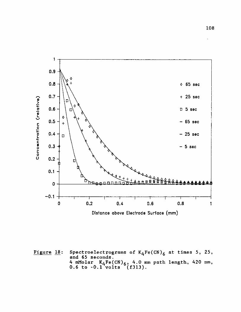
Co

ncen

trati

on

(r

ela

tiv

e)

108

0.9

0.8 0 65 sec

0.7 + 25 sec

0.6 □ 5 sec

0.5 - 65 sec

0.4 - 25 sec

0.3 - 5 sec

0.2 -

0.1 -

+ +

0.1

0 0.2 0.4 0.6 0.8Distance above Electrode Surface (m m )

Figure 18: Spectroelectrograms of K^Fe(CN)g at times 5, 25,and 65 seconds.4 mMolar KAFe(CN)6 , 4.0 mm path length, 420 nm, 0.6 to -0.1 volts (f313).

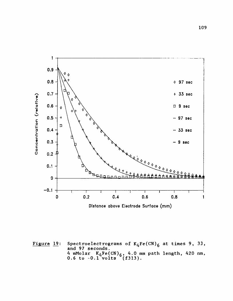
Co

ncen

trati

on

(r

ela

tiv

e)

109

0.9 -

0.8 - 0 97 sec

0.7 - + 33 sec

0.6 - □ 9 sec

0.5 - 97 sec

0.4 - - 33 sec

0.3 - - 9 sec

0.2 J]

0.1 -

- 0.1

0 0.2 0.4 0.6 0.8Distance above Electrode Surface (m m )

Figure 19: Spectroelectrograms of K^Fe(CN)g at times 9, 33,and 97 seconds.4 mMolar KAFe(CN)/-, 4.0 mm path length, 420 nm, 0.6 to -0.1 volts (f313).

Co

ncen

trati

on

(r

ela

tiv

e)

110

0.9 -

0.8 - 0 129 sec

0.7 - + 49 sec

0.6 - □ 17 sec

0.5 - - 129 sec

0.4 - - 49 sec

0.3 - - 17 sec

0.2 -

0.1 - o o

- 0.1

0.80.2 0.60 0.4

Distance above Electrode Surface (m m )

Figure 20: Spectroelectrograms of K^Fe(CN)g at times 17,65, and 129 seconds.4 mMolar KAFe(CN)g, 4.0 mm path length, 420 nm,0.6 to -0.1 volts (f313).

Illaverage correlation index. The differences tend to be quite small, due to the relative insensitivity of the theoretical­

ly calculated concentration profile to the diffusion coeffi­cients. For example, a product diffusion coefficient of 6.0 x 10“^cm^/sec gives an average correlation index of 0.99866, while 7.0 x 10“^cm^/sec yields a value of 0.99887. The dif­fusion coefficient value for the quininonediimine that gavethe highest correlation index (0.999061) is 6.58 x

fi ?10 cm /sec. This provides an excellent fit to the experi­

mentally obtained concentration profile. It should be noted

that the data points at distances of 0 and 25 microns from

the electrode surface were not used in this calculation based on the theoretical diffraction results of section 2.2.3. The measured concentration profile at 257 seconds is

given in Figure 24 to show the deviation from theory that is seen at longer times.

An alternative way to get the product diffusion coeffi­cient (Dp) from this data would be by a direct point by

point calculation. The same equations that are used to obtain the theoretical concentration profiles could be used to get the value. While it is not possible to solve for Dp in the integral of equation 3-5 or in the Maclaurin expan­

sions of equations 3-6 and 3-7, the value of D can berguessed for each position above the electrode surface and

Co

nc

en

tra

tio

n

(re

lati

ve

)

112

1 sec

- 17 sec

- 65 sec

0.4 -

0.3 -

- 0.1

0.4 0.6 0.80.20Distance above Electrode Surface (mm)

Figure 21: Spectroelectrograms of o-Tolidine at times 1,17, and 65 seconds. 0.1 mMolar o-Tolidine in0.1 M KC1/0.1 M H C l . 2.0 mm path length, 437nm, 0.1 to 0.8 volts, (o_ti4).

Co

nc

en

tra

tio

n

(re

lati

ve

)

113

0.9 -

0.8 - - 5 sec

0.7 - - 33 sec

0.6 - 97 sec

0.5 -

0.4 i

0.3

0.2 -

0.1 -

a n n n n n n n

-o .i

0.2 0.4o 0.6 0.8Distance above Electrode Surface (mm)

Figure 22: Spectroelectrograms of o-Tolidine at times 5,33, and 97 seconds.

Co

nc

en

tra

tio

n

(re

lati

ve

)

114

0.9 -

0.8 - - 9 sec

0.7 - - 49 sec

0.6 - - 129 sec

0.5 -

0.4 -

0.3 -

0.2 -

0.1 -

&43 a □ □ d p.a □ □ n trg-frtji ijjdid iftftijnjujnj]

-0.10 0.2 0.4 0.6 0.8

Distance above Electrode Surface (mm)

Figure 23: Spectroelectrograms of o-Tolidine at times 9,49, and 129 seconds.

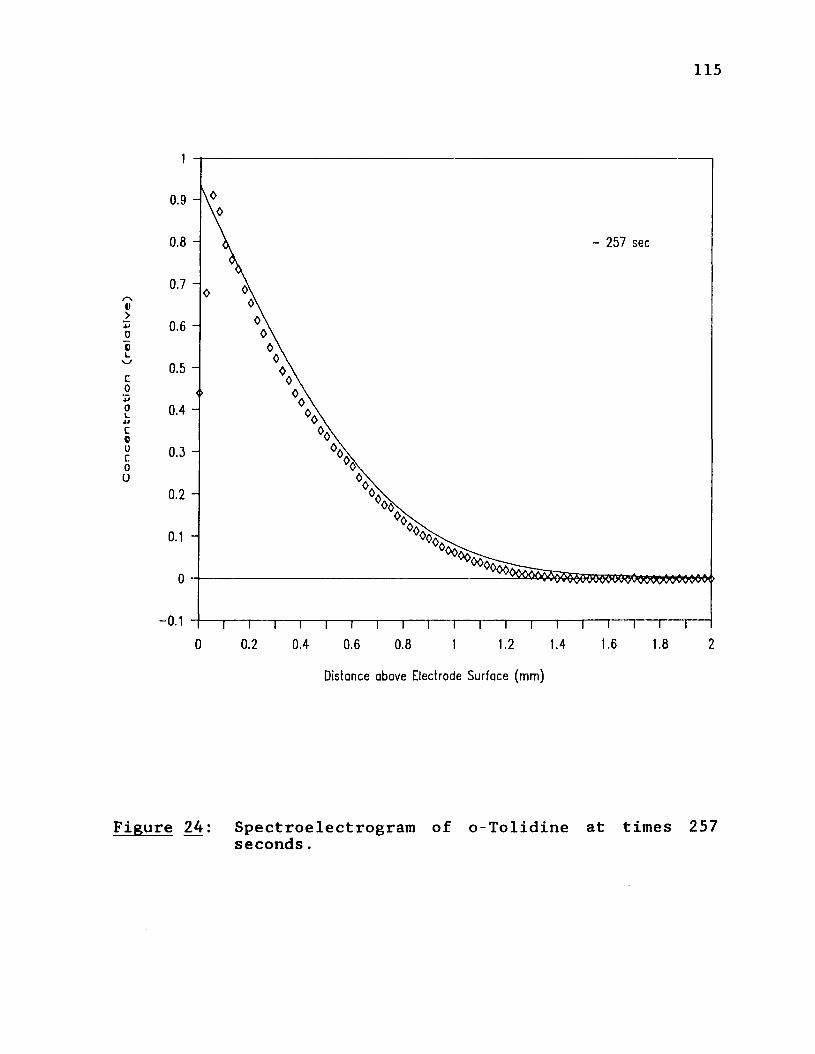
Co

nc

en

tra

tio

n

(re

lati

ve

)

115

0.9 -

0.8 - - 257 sec

0.7 -

0.6 -

0.5 -

0.4 -

0.3 -

0.2 -

0.1 -

-0.10.2 1.6 1.8 20 0.4 0.6 1.2 1.40.8

Distance above Electrode Surface (mm)

Figure 24: Spectroelectrogram of o-Tolidine at times 257seconds.

116the resulting concentration at that distance calculated and

compared to the measured value. The guessed value of D isr

increased or decreased repeatedly until the calculated con­centration is arbitrarily close to the measured value. This method has the severe disadvantage that the resultant calcu­

lated concentration profile line that passes exactly through a single experimentally measured data point may be a very bad fit over the entire collection of data points measured at that specific time. In fact, for a given reactant diffu­

sion coefficient the family of theoretical concentration profile curves that correspond to differing product diffu­sion coefficients all pass through a common point at some distance from the electrode surface. A measured value near

this shared point that is off only slightly will produce a

calculated Dp that is very far away from the actual value.

Also a point that is slightly off of the baseline at a dis­tance above the actual diffusion layer will give a high cal­culated product diffusion coefficient at that position and a

measured value below the baseline (negative) could not be used in this method at all.

An example of this method of calculating the product dif­

fusion coefficient is given in Table 7. The product diffu­sion coefficient is calculated for concentration values greater than 0.02 concentration units. These values were

117calculated using a BASIC program very similar toCONCPROF.BAS (Appendix E), that reads a measured concentra­

tion data file and produces a product diffusion coefficient for each point. The simple average Dp from the calculations for the 20 data points in this table is 6.42 x 10"^cm^/sec.The correlation index method of calculating Dp tends toweigh the values nearer to the electrode surface, which is an advantage because these data points actually carry more of the analytical signal. Due to the limitations discussed,

it was decided that the correlation index method of calcu­

lating the product diffusion coefficient was more appropri­

ate .

3.5.3 SummaryFrom these measurements it can be stated that the laser/

photodiode array system is effective in measuring the forma­

tion of concentration gradients and therefore performs well as a spectrophotometer that can resolve concentration as a function of both time and distance. It has been shown to be useful in the measurement of diffusion coefficients in a rigidly controlled electrochemical system. In addition, samples can be measured of at least 0.4 cm thickness and

quiet solution conditions can be maintained for at least 120

seconds. These latter facts are important to be able to

measure transport across membranes, as will be described in the next chapter.

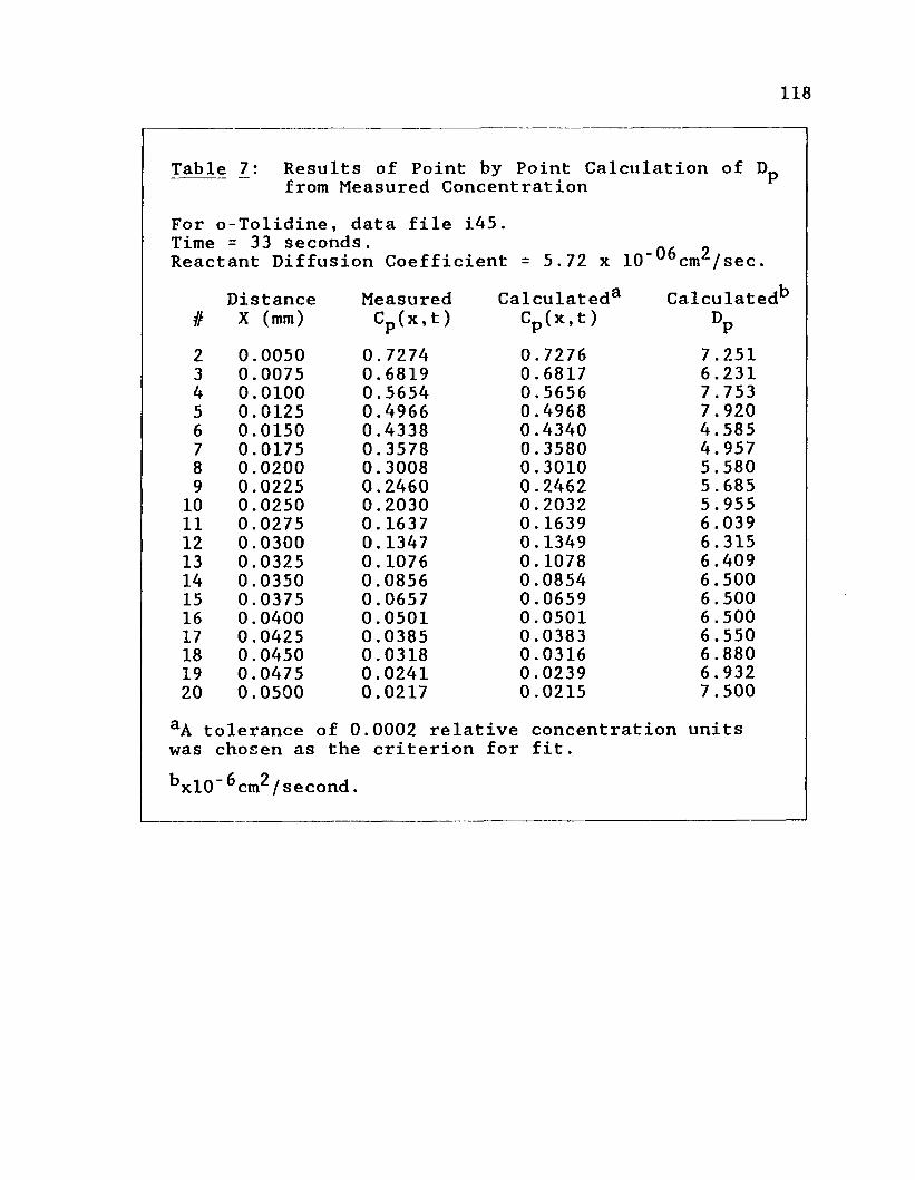
118

Table 7: Results of Point by Point Calculation of Dfrom Measured Concentration

For o-Tolidine, data file i45 . Time = 33 seconds.Reactant Diffusion Coefficient = 5.72 x 1 0 " ^ c m ^ / s e c .

Distance Measured Calculated3 Calculat# X (mm) Cp (x,t) Cp (x,t) DP2 0.0050 0.7274 0.7276 7.2513 0.0075 0.6819 0.6817 6.2314 0.0100 0.5654 0.5656 7.7535 0.0125 0.4966 0.4968 7.9206 0.0150 0.4338 0.4340 4.5857 0.0175 0.3578 0.3580 4.9578 0.0200 0.3008 0.3010 5.5809 0.0225 0.2460 0.2462 5.685

10 0.0250 0.2030 0.2032 5.95511 0.0275 0.1637 0.1639 6.03912 0.0300 0.1347 0.1349 6.31513 0.0325 0.1076 0.1078 6.40914 0.0350 0.0856 0.0854 6.50015 0.0375 0.0657 0.0659 6.50016 0.0400 0.0501 0.0501 6.50017 0.0425 0.0385 0.0383 6.55018 0.0450 0.0318 0.0316 6.88019 0.0475 0.0241 0.0239 6.93220 0.0500 0.0217 0.0215 7.500

A tolerance of 0.0002 relative concentration unitswas chosen as the criterion for fit

^xlO'^cm^/second.

Chapter IVAPPLICATION TO STUDIES IN MEMBRANE TRANSPORT

4.1 Theory

When a semi-permeable membrane barrier creates an abrupt incongruity between two solutions, diffusion driven trans­port spontaneously occurs from the region of higher chemical potential to the region of lower chemical potential. This natural tendency toward equilibrium is stated as the Second Law of Thermodynamics [87]. The result is the time depen­

dent formation of a concentration gradient on each side of

the membrane. The solution of higher chemical potential

(higher concentration) is termed the donor cell or compart­

ment and the solution of lower chemical potential is called the receiving cell. The purpose of this portion of the

research is to measure not only the bulk transport of a giv­

en species across a membrane barrier, but also to visualize the entire concentration gradient as it forms on both sides of the barrier.

The mathematical treatment of flux across an interface is simplified if conditions are rigidly maintained to restrict

- 119 -

120mass transport to diffusion. The first condition is the absence of mechanical stirring or convection. In particu­lar, the transport cell must be isolated from room vibra­

tions. Secondly, the temperature must be constant during the transport time period of interest and must be homogene­ous within the solutions. Thirdly, migration due to elec­trical gradients which are caused by the unequal distribu­

tion of a charged species must be effectively eliminated from contributing to the total transport of the species of interest. The first and second conditions are met by proper

instrumental selection and set-up. The floating optical

table used to hold all of the experimental equipment effec­

tively reduces the conductance of room vibrations to the solution cells. Use of a laser with a small pulse width as the light source dramatically decreases the introduction of

heat into the solutions, minimizing temperature effects. Migration due to the electrical gradients is controlled by the use of a supporting electrolyte, homogeneously present in both donor and receiving solutions. If the electrolyte

is present at a 100:1 ratio, by charge, to the species of interest, approximately 99% of the current needed to balance the charge discrepancy is carried by the electrolyte.

Equations describing diffusion controlled flux across the

semi-permeable barrier can be derived from Fick's Laws of

121Diffusion for the solutions on each side of the membrane if sufficient boundary conditions can be defined and experimen­tally met. It should be pointed out that these conditions and therefore this derivation closely parallels the solution of the diffusion equation for a potential step at a planar electrode for an electrochemical reaction (see Chapter III).1. For each compartment the initial condition is for

homogeneous solutions. The donor compartment will

have a chosen concentration of the species of interest and the receiving compartment will have none of this species.

2. For both compartments the semi-infinite conditionapplies. This states that at some distance away from the membrane the initial concentration condition still exits. In other words the diffusion layer cannot run

into any walls that restrict its growth.3. The third condition is that the surface concentration

of the transported species must be known at all times after the onset of flux. This can be deduced by con­

sidering the following cases. Since the species

itself or the background solution it comes in contact

with does not change during the course of an experi­ment, overall diffusion to and from the membrane is

equal but opposite. Before the onset of flux the

122concentration on the donor side of the membrane sur­face is assigned a value of one and on the receiving side the concentration is zero. At the onset of flux the concentration at the interface of these two solu­

tions (actually in the pores of the membrane) is an

equal mixture of these two solutions and would be one- half of the original donor bulk concentration (the average of the two solutions' concentrations), since

the two solutions are equally contributing at this

point. Because of the symmetrical but opposite diffu­sion to and from this plane, its concentration remains constant at this value throughout the experiment. If the solutions were to be allowed to come to equilibri­um, assuming finite, equal compartment sizes, the

final concentration in this plane (and at all points in both solutions) would be this value.

By applying these boundary conditions and using the

Laplace transform the following concentration profile equa­

tions can be derived. In the receiving cell the concentra­tion as a function of time after the onset of flux and dis­

tance from the membrane surface is:

C (x,t) = 1/2 Cd {1 - erf(-----------------------eq.4-12 (D t)1'2

123where Cr (x,t) is the concentration in the receiving compart­ment as a function of position, x, and time, t, and D is the

diffusion coefficient. In the donor cell the analogous equation is:

Cd (x,t) = 1/2 Cd {1 + erf (------} eq.4-22 (D t)1'2

where Cd (x,t) is the concentration in the donor compartment.

Using the Maclaurin expansion approximations described in Section 3.1.2 the theoretical concentration profiles can be

calculated at a selected time and distance away from the

interface for a given species diffusion coefficient. This is demonstrated in a BASIC program, THEORMT.BAS, included as

Appendix H. An example profile is shown in Figure 25 for a- fk 9species of diffusion coefficient 5 x 10 cm^/sec at times

15, 30, 60, 90, and 120 seconds after the onset of flux.

An interesting result of diffusion controlled flux is

that the profile curves can be further evaluated by inte­

grating the areas on each side of the membrane to get a total amount transported at a given time. This is done for the receiving side by simply summing the points in a single

curve up to the membrane surface. For the donor side the points are summed and this is subtracted from the number of

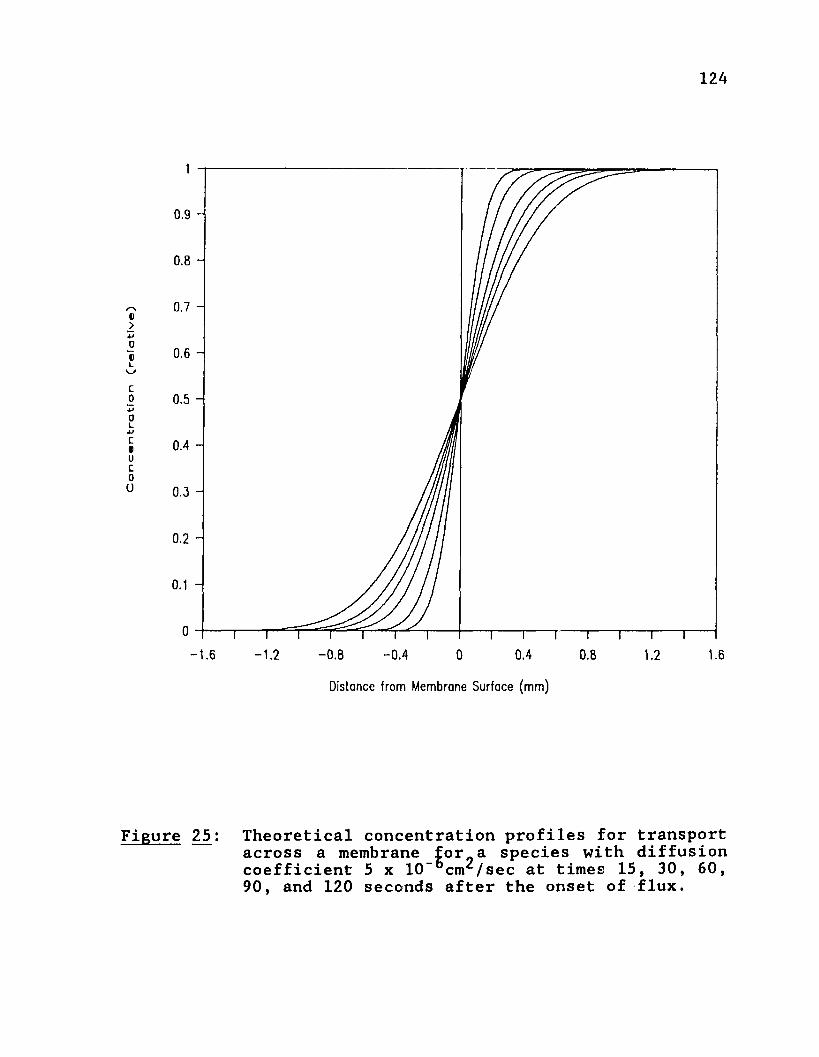
Co

nc

en

tra

tio

n

(re

lati

ve

)

124

1

0.9

0.8

0.7

0.6

0.5

0.4

0.3

0.2

0.1

0-1 .6 -1 .2 -0 .8 -0 .4 0 0.4 0.8 1.2 1.6

Distance from Membrane Surface (mm)

Figure 25: Theoretical concentration profiles for transportacross a membrane for a species with diffusion coefficient 5 x 10"°cm^/sec at times 15, 30, 60, 90, and 120 seconds after the onset of flux.

125points times the concentration in the bulk solution on that side to get the amount that has left this side of the mem­brane system at a given time. The results of the integra­tions should yield the same number for both sides of the barrier, because what is lost from one side is gained on the

other. The results of this calculation are demonstrated in

Figure 26 for five different species with diffusion coeffi-ft )cients ranging from 1 to 10 x 10 cm^/sec.

Additionally the total amount transported at a chosen

time, J(t), can be related to several other parameters:

J(t) a A C ^ D / t ) 1/2 eq.4-3

■>vwhere A is the cross-sectional area for transport, is the initial bulk concentration in the donor cell, and D is the diffusion coefficient of the species. These curves can be further evaluated by plotting the integrated amount, J(t),

multiplied times the square root of time against time. This

yields a linear plot that has a slope proportional to the

square root of the diffusion coefficient. This is shown in Figure 27.

Furthermore, a series of theoretical membrane transport

diffusion profiles for several diffusion coefficients can be

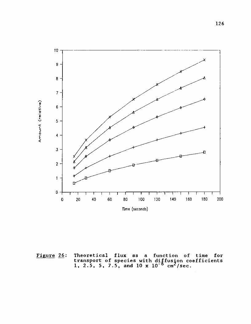
Am

ou

nt

(re

lati

ve

)

126

10

9

8

7

6

5

4

3

2

o140 160 180 20010040 120

Time (seconds)

Figure 2 6 : Theoretical flux as a function of time fortransport of species with diffusion coefficients 1, 2.5, 5, 7.5, and 10 x 10 cm /sec.

Am

ou

nt

* S

QR

T(t

ime

)

127

Time (seconds)130

120 -

100 -

80 -

70 -

60 -

50 -

40 -

30 -

20 -

10 -

17015011 0 13050 70 903010Time (seconds)

Figure 27: (Flux)*(time) ^ as a function of time fortransport of a theoretical species with diffu­sion coefficients 1, 2.5, 5, 7.5, and 10 x10~°cm^/sec.

128used first to generate the integrated flux as a function of time, and then the J ( t ) * t ^ ^ plots. This series of plots

can be evaluated for slope and this series of slopes can be plotted against the square root of the diffusion coefficient that was used to produce each one, to get another linear plot. This is the upper line depicted in Figure 28. The equation of this line can be used to evaluate the experimen­tally generated membrane transport diffusion profiles. The slope of the J(t)*t^/^ plot from the experimental data can be used to calculate the effective diffusion coefficient for

the species crossing the particular barrier used in an

experiment.

The experimental data can be evaluated only to within 75 microns of the membrane surface, on each side. Fortunately

when the same restriction is applied to the theoretical

data, it still yields a linear J(t),vt^/^ plot. This is the lower line of Figure 28. The slopes of these lines are the

same, but the intercepts differ. The lower line is the one used to evaluate the experimental data. It yields the fol­lowing equation:

(measured slope) = 223.5 * - 0.1103 eq.4-4

The correlation coefficients for the fit of these calculated

points to the least squares lines are 0.99999, due to round­

ing error.

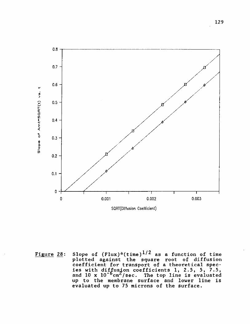
Slo

pe

of

Am

t*S

QR

T(t

)

129

0.8

0.4 -

0.3 -

0.0030 0.0020.001

SQRT(Diffusion Coefficient)

Figure 28: Slope of (Flux)*(time) / as a function of timeplotted against the square root of diffusion coefficient for transport of a theoretical spec­ies with diffusion coefficients 1, 2.5, 5, 7.5, and 10 x 10”6cm /sec. The top line is evaluated up to the membrane surface and lower line is evaluated up to 75 microns of the surface.

130An effective diffusion coefficient or permeation constant

must be used because of differences between the theoretical

model and the experimental system. The theoretical model assumes a full cross-sectional area available for transport,

allowing linear diffusion only. The artificial membranes described in the next section are thin impermeable sheets

with pores through which transport can occur. Only a frac­tion of the total cross sectional area is actually available for transport and near the membrane, diffusion will be non­

linear. Irregardless of this fact, the experimental results fit the theoretical model chosen quite well.

4.2 Nuclepore Membranes

Nuclepore (R) membranes (Nuclepore Corp., Pleasanton, CA)

were chosen to perform the initial membrane transport stud­

ies because of their favorable physical and chemical proper­

ties. They are track-etched micropore polycarbonate sheets

that are smooth, flat, thin, and chemically inert. The mem­

branes are 6-10 microns thick, yet are relatively sturdy. They have a sharply defined pore size that is produced by a two step process of irradiation and etching. The membrane material is biologically inert, non-hygroscopic, and and exhibit low non-specific adsorption. They have excellent chemical and thermal stability. In addition, Nuclepore

131membranes are available in a variety of pore sizes, 0.015 to 10 micron in diameter, as 13 or 25 millimeter disks. The

geometrically well-defined pore size, density, and capillary shaped pore structure make them well suited as model mem­branes for theoretical and applied research [88,89].

The membranes are presoaked in the background solution overnight before use. This decreases the time needed to reach a steady-state in transport as described by Chien [89].

4.3 Membrane Transport Cell Assembly

To study membrane transport, a cell was designed to meet these minimal requirements:1. The membrane is held securely in place, flat, and with

an appreciable surface area available for transport

between two compartments.2. The walls of the cell should be perpendicular to the

membrane so that transport can be limited to linear

diffusion up to the surface.3. Two parallel walls must be flat and optically trans­

parent down to the membrane surface on both sides of the membrane.

4. The cell assembly must be water tight and access to at

least one of cell compartments is necessary to be able

to introduce the transporting species.

132To meet these criteria, which parallel the spectroelec-

trochemical cell requirements, a cell design similar to the spectroelectrochemical cell was chosen. The cell used con­sists of two pieces of rectangular bore glass tubing, 2 mm by 6 mm inner diameter (Wilmad WR-0206) polished to a high

degree of smoothness and flatness, as described in section

3.2.1 . The lower compartment is sealed at the bottom with

clear silicone Windshield Glass Seal (General Electric, Waterford, N.Y.). The membrane is sandwiched between the polished surfaces to define the two cell compartments. The

glass tube/membrane/glass tube arrangement must be held together securely and straight. Uneven pressure could result in cell leakage. A good seal was achieved by tension

fitting the assembly together with two pieces of polycarbo­nate rod machined to the specifications given in Figure 29. The two pieces described fit together to form a approximate­ly 4 inch long by 1/2 inch diameter cylinder, with a vari­

able length inside compartment that has an 8 mm by 4 mm

cross-section. The two pieces of glass tubing and the mem­

brane fit in this chamber and pressure is applied only in

the vertical direction. Also the area all around the inter­

face is machined out so that capillary action will not draw solution out of the cell.

133

PieceSide View; .37 J5J_ - J

- 2 / / -

-IT­

'S

Top View*. ■n

Piece *2S id e V i e w

.15.15

3 .13'

Top V iew :.

.521 .2 9 5 .461< f

Figure 2 9 : A schematic diagram of the membrane transportcell holder.

134To hold the two polycarbonate pieces together a nylon

cylinder is constructed as follows. A 1 inch diameter nylon

rod is drilled through its length with a 31/64 inch drill.

This is slightly enlarged with a variable 1/2 inch reamer to tightly fit the polycarbonate assembly. A 27/64 inch hole is drilled 1.2 inches from one end of the cylinder, perpen­dicular to its length, to serve as the light path. Twosmall holes are drilled 0.7 and 1.7 inches from the same endof the cylinder through one side, parallel to the light pathaperture. These are tapped 6-32 to receive 1 cm nylon

screws that will hold the cell in place. The other side of

the cylinder is milled out to form a 1.25 by 0.65 inch depression, 0.15 inches deep in the area around the light

path aperture. This allows the diode array chip to recess into the cell holder, minimizing the distance between the cell and the detector.

The following procedure is used to assemble and fill the cell and holder. The membrane being used is cut so that it fits on top of the rectangular bore glass tube, covering the opening, but not sticking out over the edges. The tube is 2 mm by 6 mm inner diameter with a wall thickness of about 1 mm, so the membrane must be about 2.5 mm by 6.5 mm with somewhat rounded edges. The bottom cell compartment is

filled with background solution and the membrane is layered

135on top of this, carefully centering it and being sure no air bubbles are present. This is placed in the bottom part of the polycarbonate pieces and the other glass compartment (empty) is carefully set on top of this. The top polycarbo­nate piece is pushed half way into the nylon holder and the

bottom part with the glass half-cells in it is slid into place beneath this. The entire assembly is moved up into

place in the nylon holder so that the light paths line up. The glass cells are arranged so that the 2 mm inner cross

section serves as the light path. The polycarbonate pieces

with the cell assembly are secured into place with the two nylon screws. The assembled membrane transport cell and

cell holder is shown in Figure 30 and the disassembled mem­

brane transport cell assembly and holder is shown in Figure 31. The top compartment can be filled with solution through the hole in the polycarbonate piece with a Pasteur pipette.

136

Figure 30: The membrane transport cell assembly and cellholder.

137

138

Figure 31: The disassembled membrane transport cell assem­bly and cell holder.

1404.4 Reagents

Analytical reagent grade chemicals were used without further purification. Methyl orange, sodium p-dimethylaminoazo-

benzenesulfonate, (Aldrich AM-0909LJ) was used as the spec­ies whose transport would be monitored. Its high molar absorptivity over a wide pH range makes it well suited for this purpose. Phosphate buffers of pH 3, 5, 7, and 10 and a

final ionic strength of 0.2 molar were used as the back­ground solutions. Solution of 0.22 molar sodium dihydrogen

phosphate (Mallinckrodt X R M ) , disodium hydrogen phosphate

(Mallinckrodt KTAY), and trisodium phosphate (J. T. Baker

41512) were first prepared. To prepare the pH 3 phosphate buffer a portion of the N a ^ P O ^ solution was adjusted with

about 0.4 mL of phosphoric acid per liter of solution. A Sargent-Welch 6050 pH Meter was used to monitor the pH as the concentrated acid was slowly added. The pH 5 and 7

buffers were prepared by starting with a measure of the N a ^ P O ^ and adding sufficient Na2HP0^ to get the desired pH, as monitored with the pH meter. The pH 10 buffer was pre­pared by starting with Na2HP0^ and adding enough of the

Na3P0^ solution to get the desired pH. This produces 0.22 molar solutions of each of the buffers that when used to

dilute 10 mL of methyl orange in water to 100 mL of final

solution volume a final background ionic strength of 0.20 molar is obtained.

141Stock reference standard methyl orange solution was pre­

pared by accurately weighing about 0.17 gm of 97% methyl orange crystals and dissolving with double distilled water.

This is serial diluted with water or the appropriate buffers to produce 5 x 10”^ and 5 x 10'^ molar solutions of methyl

orange. These solutions were assayed spectrophotometrically

each day to determine the pH dependent molar extinction coefficient and ensure stability.

4.5 Experimental Procedure

4.5.1 General ProcedureTwo series of experiments were conducted to examine the

transport process. The transport of methyl orange across a Nuclepore membrane at different pHs was examined and the transport of methyl orange across Nuclepore membranes of

various pore diameters was studied.

The transport cell was prepared and assembled as

described in section 4.3 . The bottom half of the transport

cell was filled with background solution (the different

phosphate buffers). The membrane was carefully cut with a

razor blade to fit over the solution without sticking out over the edges of the glass cells. The membrane is layered over the solution, the cell is assembled, and the top

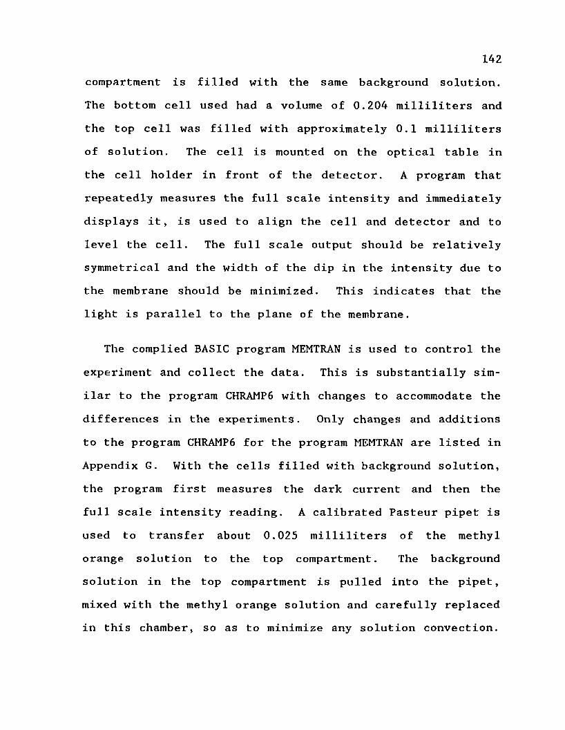
142compartment is filled with the same background solution.

The bottom cell used had a volume of 0.204 milliliters and the top cell was filled with approximately 0.1 milliliters of solution. The cell is mounted on the optical table in the cell holder in front of the detector. A program that repeatedly measures the full scale intensity and immediately

displays it, is used to align the cell and detector and to level the cell. The full scale output should be relatively symmetrical and the width of the dip in the intensity due to the membrane should be minimized. This indicates that the light is parallel to the plane of the membrane.

The complied BASIC program MEMTRAN is used to control the

experiment and collect the data. This is substantially sim­

ilar to the program CHRAMP6 with changes to accommodate the differences in the experiments. Only changes and additions

to the program CHRAMP6 for the program MEMTRAN are listed in Appendix G. With the cells filled with background solution,

the program first measures the dark current and then the full scale intensity reading. A calibrated Pasteur pipet is

used to transfer about 0.025 milliliters of the methyl orange solution to the top compartment. The background solution in the top compartment is pulled into the pipet, mixed with the methyl orange solution and carefully replaced in this chamber, so as to minimize any solution convection.

143The same time interval as was chosen to collect the data is waited to start experimental data collection. The data is collected and the intensity is normalized to the full scale value automatically. The data is stored in random access files on the computer's hard disk. As in the electrochemi­cal experiments, these data files can be converted to either Lotus or SAS compatible data files for further data reduc­tion.

4.5.2 Methyl Orange Transport at Different pH Values

Methyl orange transport across 0.2 micron Nuclepore membrane was measured at various pH values. Phosphate buffers of pH 3, 5, 7, and 10 at 0.2 molar ionic strength were used as

background solutions. The electronic absorbance spectrum of methyl orange in each of these solutions was measured from 200 to 600 nm with an IBM Instruments UV-Visible Spectropho­tometer (IBM Instruments, Danbury, Conn.). The dye laser

was tuned to the maximum absorbance wavelength for the solu­tion being measured. The dye laser was periodically cali­brated with an Instruments SA, Inc. DH20A monochromater

(Metuchen, N.J.), using the nitrogen laser at 337.1 nm as

the standard wavelength. For pH 5, 7, and 10 465 nm is the

Xmax> with a molar extinction coefficient of 25200

(cm-M)-^. At pH 3 the wavelength of maximum absorption is

at 503 nm with a molar extinction coefficient of 34300

144(cm-M)"^. Methyl orange is used as a pH indicator. Over the pH range 3.2 to 4.4 it changes from a pink or red color

to yellow, due to the protonation of a highly conjugated phenyl sulfate group. At low pH the red form of methyl orange predominates.

4.5.3 Methyl Orange Transport Across Nuclepore Membrane of Various Pore Size

Methyl orange transport across various pore sizes of Nucle­

pore membrane was measured in phosphate buffer of pH 7 and 0.2 molar ionic strength. The dye laser was tuned to 465 nm. The cell was set up as described above and the program

MEMTRAN was used for the data collection. Four experiments for each membrane pore size were collected so averaging could be performed to increase precision of the final flux

measurements.

4. 6 Results and Discussion

The experimental results for the transport of methyl orange

across a Nuclepore membrane of 0.2 micron pore size is shown

in Figure 32. The initial bulk concentration of methyl orange in the donor compartment was approximately 1 x 10"^

molar. The concentration in Figure 32 is plotted as a frac­tion of this value. This is done so that slightly different initial bulk concentrations can be directly compared. The concentration profiles are shown at 30 second intervals.

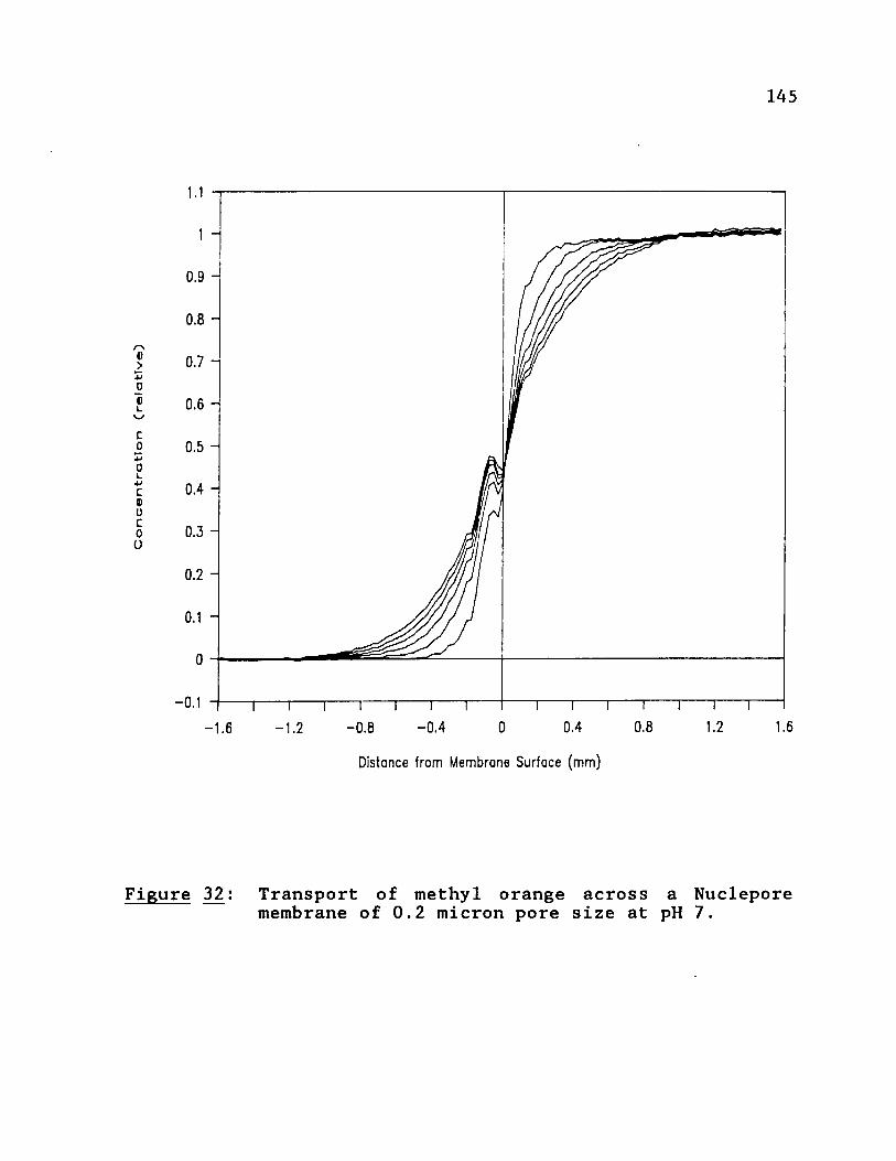
Co

nc

en

tra

tio

n

(re

lati

ve

)

145

0.9 -

0.8 -

0.7 -i

0.6 -

0.5 -

0.4 -

0.3 -

0.2 -

0.1 -

- 0.1

0.8 1.2 1.6-0.4 0 0.4- 0.8- 1.21.6Distance from Membrane Surface (mm)

Figure 3 2 ; Transport of methyl orange across a Nuclepore membrane of 0.2 micron pore size at pH 7.

146The evaluation procedure outlined in section 4.1 was car­

ried out for each experimental data set collected. The flux

plot for the experiment of Figure 32 is shown in Figure 33. This depicts the total amount of methyl orange that has crossed the membrane at the various times. Both the top and bottom compartments are shown here. These should be the same and as can be seen, are in fact very close.

When the amount that has crossed the membrane at a given

time is multiplied by the square root of time and plotted

against that time, the graph in Figure 34 is obtained. The

slope for these two lines are 0.361 and 0.382 . When theseare evaluated using equation 4-4, from Figure 28 the value

of the permeation constant can be calculated. The results- C\ A 9for this experiment are 4.45 x 10 and 4.85 xlO cm /sec.

This range represents the experimental uncertainty in these

measurements. The remaining permeation constants presented are an average of the top and bottom compartment values.

Table 8 gives the permeation constants for the transport

of methyl orange across 0.2 micron Nuclepore membrane in 0.2 M phosphate buffer at the pH indicated. The slight varia­

tions could be due to actual small differences in the diffu­

sion coefficient of methyl orange at the different condi­

tions or to experimental variability. This experiment shows

that the membrane is stable over this pH range.

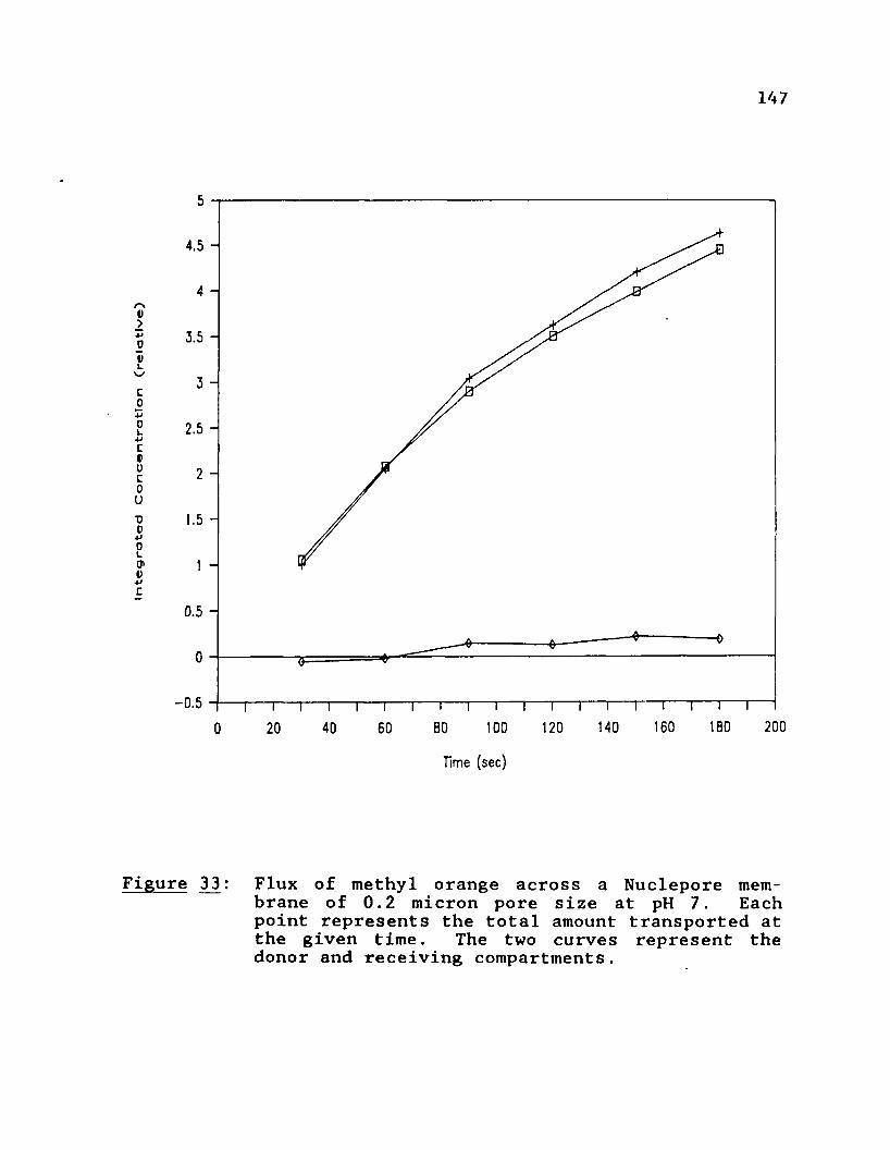
Inte

gra

ted

C

on

ce

ntr

ati

on

(r

ela

tiv

e)

147

5

4.5

4

3.5

3

2.5

2

1.5

1

0.5

0

-0.50 20 40 60 80 100 120 140 160 1B0 200

Time (sec)

"I r 1------ 1— T i— i— I— r

Figure 3 3 : Flux of methyl orange across a Nuclepore mem­brane of 0.2 micron pore size at pH 7. Each point represents the total amount transported at the given time. The two curves represent the donor and receiving compartments.

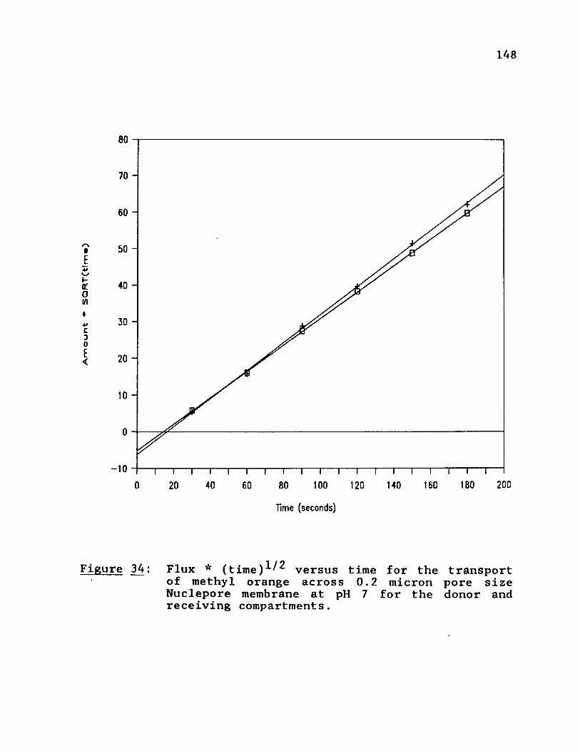
Am

ou

nt

* S

QR

T(t

lm«

)

148

70 -

60 -

50 -

40 -

30 -

20 -

10 -

-1 0

20018040 80 100 140 1600 20 60 120

Time (seconds)

Figure 34: Flux * (time)^/^ versus time for the transportof methyl orange across 0.2 micron pore size Nuclepore membrane at pH 7 for the donor and receiving compartments.

149

Table 8: Permeation Constants of Methyl Orange atVarious pHs

pH Slope Permeation Constant (cm /sec)3 0.382 4.85 x 10"^5 0.354 4.32 x 10'°7 0.372 4.65 x 10'°

10 0.351 4.25 x 10"6Over a 120 second measurement period, at a 75 micron distance from the membrane surface.

The permeation constant is unchanged over the concentra­tion range 1 x 10'-* to 2 x 10'^ for pH 5, 7, and 10. This

is not the case for solutions of methyl orange in pH 3 buff­

er. At pH 3 the solubility of methyl orange is less than at higher p H s . The transport of methyl orange in pH 3, 0.2 M ionic strength phosphate buffer is concentration dependent between 5 x 10'^ and 1.0 x 10'^ molar. There is no measura­ble transport above 1.0 x 10'^ molar. Transport at approxi­mately 7.5 x 10'^ molar is retarded for about the first 60

seconds and does not continue after this time. Transport at

5.0 x 1 0 ' molar continues normally throughout the measure­

ment period. This is shown in Figure 35. The top curve is

for membrane transport at the lower concentration, which

follows the pattern for methyl orange transport at the high­

er p H s . The flux times the square root of time versus time

150plot is shown in Figure 36. The lower concentration gives a linear plot as predicted by the model calculations, while

the higher concentration plot appears curved.

The reason for this concentration dependence at pH 3 is not known. It may be that the free base methyl orange

adsorbs on to the membrane surface and the salt form does

not. This could not be verified by examining the used mem­branes under a 44x microscope. No color change of the m em­brane was apparent. It could also be that small particu­lates are clogging the pores as a function of time. Thisrange is close to the limit of methyl orange solubility.

The solutions were allowed to set and no crystal formationwas noted. These solutions were further diluted to ensure that the solubility limit was not exceeded.

The results of the permeation constant measurement for

the transport of methyl orange across Nuclepore membranes of

various pore sizes is given in Table 9. Also listed are

other membrane parameters either supplied by Nuclepore [88] or calculated from their information.

The permeation constant generally increases with membrane pore size and pore area, but is not directly proportional to any of the parameters listed. The pore area is calculated

from the pore density and the pore size, assuming a

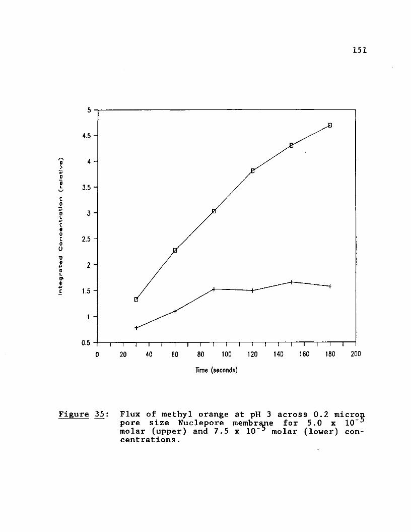
Inte

gra

ted

C

on

ce

ntr

ati

on

(r

ela

tiv

e)

151

4.5 -

3.5 -

2.5 -

0.5

200140 160 18040 100 120800 20 60

Time (seconds)

Figure 3 5 : Flux of methyl orange at pH 3 across 0.2 micronpore size Nuclepore membrane for 5.0 x 10 molar (upper) and 7.5 x 10"5 molar (lower) con­centrations .

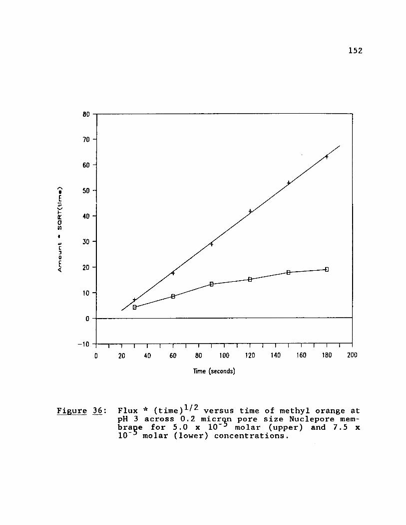
Am

ou

nt

* S

QR

T(t

lm«

)

152

70 -

60 -

50 -

40 -

30 -

20 -

10 -

- 1 0

180 200140 16080 100 12040 600 20

Time (seconds)

Figure 3 6 : Flux * (time) ^ versus time of methyl orange atpH 3 across 0.2 micron pore size Nuclepore mem­brane for 5.0 x 10”5 molar (upper) and 7.5 x 10“5 molar (lower) concentrations.

153

Table 9: Permeations Constants of Methyl Orange forTransport Across Nuclepore Membrane ous Pore Size.

of Vari-

Pore Size # Pores Calculated Typical Permeatio(microns) per cm Pore Areaa Flow Rate Constant0.015 6 x 108 0.00106 < 0.1 1.210.05 6 x 108 0.0118 0.2 3.350.1 3 x 108 0.0236 8 3.790.2 3 x 108 0.0942 15 4.771.0 2 x 107 0.1571 350 5.602.0 2 x 106 0.0628 500 3.025.0 4 x 105 0.0785 2000 3.39

10.0 2 x 105 0.0785 2000 2.89

B

acm^ of pore area per cm^ of membrane.

10”^cm^/sec.

perfectly round pore. The mean pore size is held to a manu­

facturing tolerance range of +0% to -20% of the reported

pore size in Table 9 [88]. This adds to the uncertainty in

the data. The lack of a simple relationship between pore

size or area to the permeation constant is due to the non­

linear nature of the mass transport across this type of mem­brane .

154OTypical flow rate is for water in ml/minute/cm at 5 PSI.

This is hydrodynamic flow and is not expected to relate to the diffusion controlled transport measured here.

4.7 Summary

An initial homogenous solution containing the species of

interest is separated from a blank solution by a semi- permeable artificial membrane. As the species diffusions across the membrane the laser/photodiode array spectropho­

tometer simultaneously measures the formation of the concen­tration profiles on both sides of the barrier under quiet

solution conditions. A theoretical model for these experi­

mental conditions has been developed and applied to the

measured results. The model, though somewhat empirical, fits these experimental results quite well. The effect of pH and concentration on the transport rate was studied. Over the pH range 5 to 10 and .01 to 2 mMolar methyl orange relative transport was the same. At pH 3 the transport

showed a concentration dependence. The rate of transport

was also found to be dependent on the pore area of the m em­

brane used, however a simple relationship between the physi­

cal size characteristics of the membrane and the permeation

constant was not found.

Chapter V

CONCLUSIONS

A powerful new tool for the measurement of mass transport in glass cells of 2 to 4 millimeter depth has been developed based on electronic absorption spectroscopy. A pulsed laser

system in combination with a linear photodiode array is used to produce spacially and temporally resolved concentration measurements. This has been demonstrated to be useful in

visualizing the concentration profile in the diffusion layer above an electrode surface. These measurements, of known values, were used to validate the procedure. The technique

has also been applied to the measurement of transport across

a series of artificial polycarbonate membranes, under vari­

ous solution conditions. Concentration profiles in this system reveal information relating to the species and prop­

erties of the membrane. A theoretical model was developed that is applicable to this membrane transport system. This was used to calculate a permeability constant for the trans­port of the compound across the specified membrane under the conditions chosen.

- 155 -

156This experimental technique should be useful in the study

of transport in several other systems, such as the diffusion

of a species away from a controlled release dosage form and transport of drugs and other species of biological interest across biological membranes.

Appendix A CHRAMP6.BAS

1

10 ' $TITLE: 'CHRAMP6.B A S '20 ' $LINESIZE: 132

110 ' CHRAMP.BAS130 ' Version 0.6 5-21-84 RAC140 '150 ' Chramp.bas is a program that uses a Tecmar Lab-160 ' Master to collect 128 data points from a Self-170 ' scanning Linear Silicon Photodiode Array by180 ' calling a subroutine (adc) in the assembler pro-190 ' gram SLAVE.ASM. Specifically chramp is a var-200 ' iation of the program master.bas, that is used in210 ' spectroelectrochemical experiments, particularly220 ’ chronoamperometry. It allows for faster se-230 ' quential collection of data and uses the Tecmar240 ' LabMaster D/A converter to effect the potential250 ' step of the IBM EC/225 Voltammetric Analyzer. To260 ' accomplish this, D/A channel #0 should be con-270 ’ nected to the auxiliary input of the EC/225. The280 1 Tecmar board should be in the I/O mapped mode290 ' with +/- 10 volts full scale input. The program300 ' is set up to accommodate synchronization with the310 ' triggering of the laser and to correct for fluc-320 ' uation in the laser pulse by normalizing each330 ' diode array scan to the full scale reading. The340 ' program itself is modularized into subroutines.350 ' New data is collected or old data is reviewed by360 ' using different subroutine sequences. Also an370 ' experiment can be continued.380 '

For purposes of this listing only, a line that is not num­bered is a continuation of the previous program line.

157 -

390400410420430440450460470480490500510520530540550560570580590600610620630640650660670680690700710720730740750760770780790800810820830840850860870880

158The INTEGRATION TIME of the Photodiode Array is set through the digital I/O (ports B and C) of the Tecmar LabMaster. There are 12 bits of con­trol of the integration time corresponding roughly to 0 to 333 msec (all bits low=333 msec) at about 50 KHz scan speed. Port B sets bits 0-7 and port C sets bits 8-11. Bits 12 and 13 of Port C are control bits that should be set low for normal operation. Once the integration time is set, the diode array continually scans at that rate. The multiplexed analog signal is accessed through the analog out BNC of the scan sequencer box. The actual scan speed of the array is set by hardware on the diode array board and is lim­ited to about 52 KHz by the speed of the sub­program Slave.asm. All of the experimental para­meters are stored in a pseudo-random access file (filename.inf).

The diode array is self-scanning, that is it scans continually, however the data is only read by the A-to-D converter when the scan sequencer outputs a series of pulses (from clock out of the scan sequencer box) to the external start con­version (clock in of the Tecmar box). These pulses correspond one to one with the positions in time on the analog signal that correspond to each diode. This SCAN READ rate is set by con­necting the clock out on the Tecmar box (clock 4 of the Tecmar LabMaster) to the clock in of the scan sequencer box. The scan read rate should not exceed the time necessary for the software routines in between reads (calculations, print­ing, and plotting) or scans will be lost and a read could start in the middle of a scan. In order to synchronize the pulsing of the laser with the reading of a scan, a scan is first read, which can be used as a dark current reading, then the laser is pulsed and the array is read again for the sample reading. To accomplish this three clocks are used, a master clock to control the timing between samples and two subordinate clocks to independently control the laser and the scan sequencer.The Analog-to-Digital converter must be set up before the subroutine adc is called. Initially external start conversions are disabled. Then external start conversions are then enabled, auto-incrementing is disabled and the channel

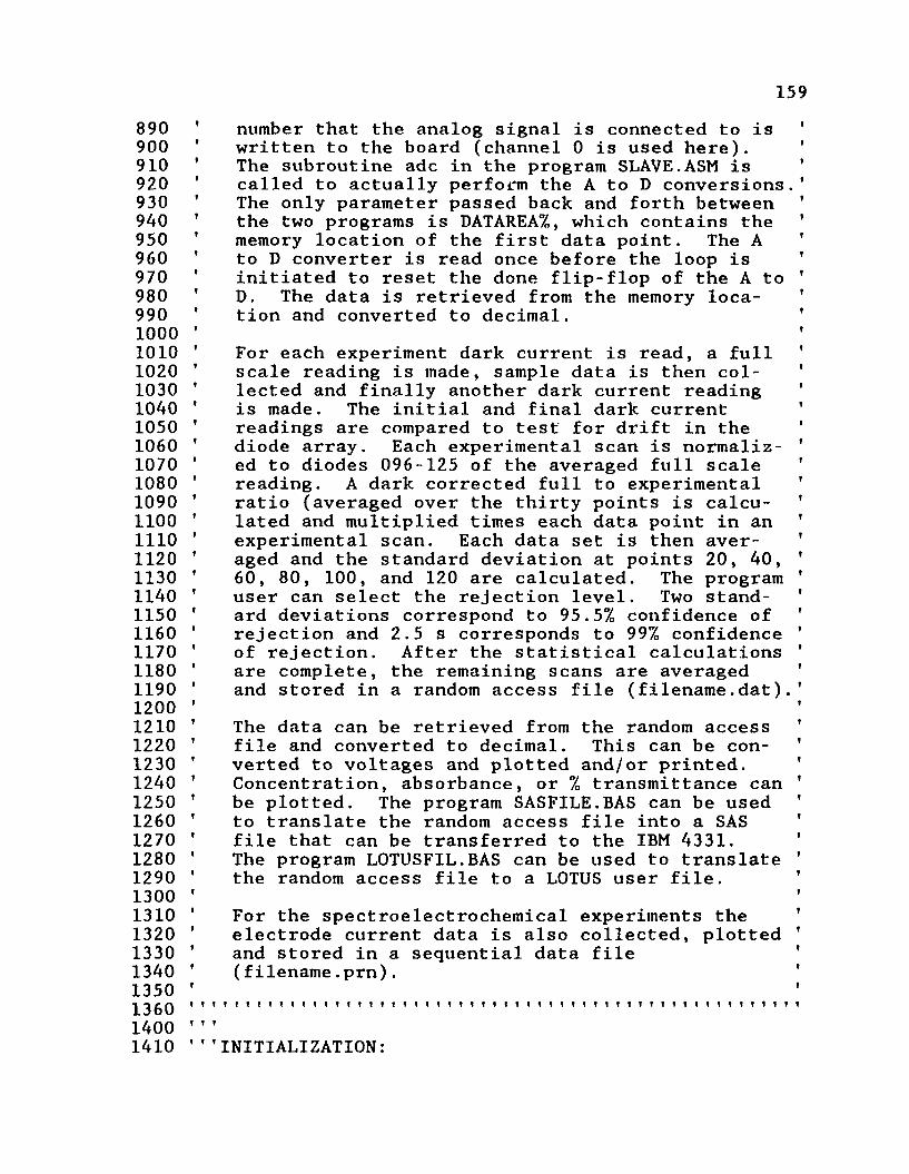
890900910920930940950960970980990100010101020103010401050106010701080109011001110112011301140115011601170118011901200121012201230124012501260127012801290130013101320133013401350136014001410

159number that the analog signal is connected to is written to the board (channel 0 is used here).The subroutine adc in the program SLAVE.ASM is called to actually perform the A to D conversions. The only parameter passed back and forth between the two programs is DATAREA%, which contains the memory location of the first data point. The A to D converter is read once before the loop is initiated to reset the done flip-flop of the A to D. The data is retrieved from the memory loca­tion and converted to decimal.

For each experiment dark current is read, a full scale reading is made, sample data is then col­lected and finally another dark current reading is made. The initial and final dark current readings are compared to test for drift in the diode array. Each experimental scan is normaliz­ed to diodes 096-125 of the averaged full scale reading. A dark corrected full to experimental ratio (averaged over the thirty points is calcu­lated and multiplied times each data point in an experimental scan. Each data set is then aver­aged and the standard deviation at points 20, 40, 60, 80, 100, and 120 are calculated. The program user can select the rejection level. Two stand­ard deviations correspond to 95.5% confidence of rejection and 2.5 s corresponds to 99% confidence of rejection. After the statistical calculations are complete, the remaining scans are averaged and stored in a random access file (filename.dat).The data can be retrieved from the random access file and converted to decimal. This can be con­verted to voltages and plotted and/or printed. Concentration, absorbance, or % transmittance can be plotted. The program SASFILE.BAS can be used to translate the random access file into a SAS file that can be transferred to the IBM 4331.The program L0TUSFIL.BAS can be used to translate the random access file to a LOTUS user file.For the spectroelectrochemical experiments the electrode current data is also collected, plotted and stored in a sequential data file (filename.prn).

f f

''INITIALIZATION:

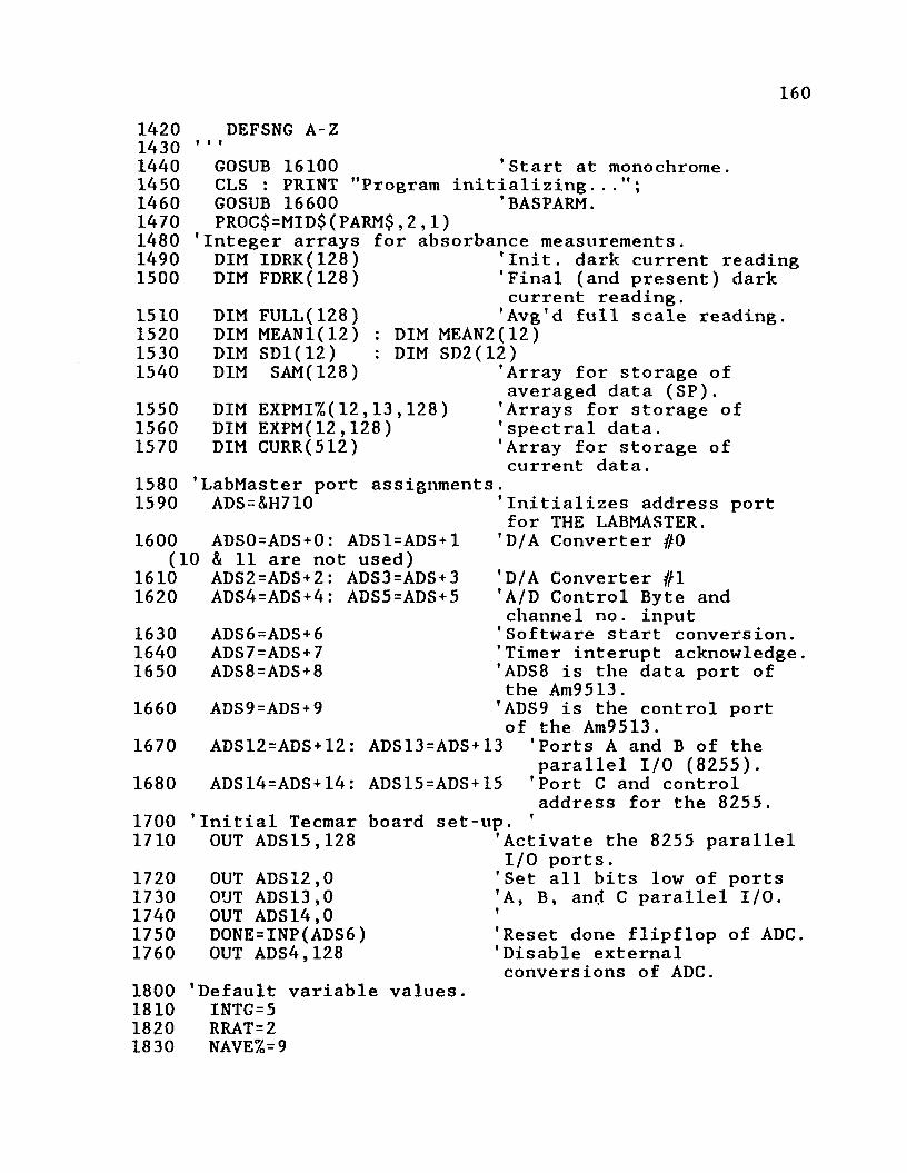
1601420143014401450146014701480149015001510152015301540155015601570

15801590

DEFSNG A-Z

monochrome **.GOSUB 16100 ’Start atCLS : PRINT "Program initializing.GOSUB 16600 ’BASPARM.PROC$=MID$(PARM$,2,1)

'Integer arrays for absorbance measurementsDIMDIM

DIMDIMDIMDIMDIMDIMDIM

IDRK(128) FDRK(128)

FULL(128) MEAN1(12) SD1(12) SAM(128)

DIMDIM

EXPMI%(12,13 ,128 ) EXPM(12,128) CURR(512)

'LabMaster port ADS=&H710

1600(10

161016201630164016501660

ADS0=ADS+0: ADS1=ADS+1 & 11 are not used)

'Init. dark current reading 'Final (and present) dark current reading.'Avg'd full scale reading.

MEAN2(12)SD2(12)

'Array for storage of averaged data (SP).'Arrays for storage of 'spectral data.'Array for storage of current data.

assignments.'Initializes address port for THE LABMASTER.'D/A Converter #0

ADS2=ADS+2: ADS4=ADS+4:ADS6=ADS+6ADS7=ADS+7ADS8=ADS+8ADS9=ADS+9

ADS3=ADS + 3 ADS5=ADS+5

'D/A Converter #1 'A/D Control Byte and channel no. input 'Software start conversion. 'Timer interupt acknowledge. 'ADS8 is the data port of the Am9513.'ADS9 is the control port of the Am9513.

1670 ADS12=ADS+12: ADS13=ADS+13

1680 ADS14=ADS+14: ADS15=ADS+15

17001710

17201730174017501760

1800181018201830

Initial Tecmar board OUT A DS15,128

OUT A DS12,0 OUT A DS13,0 OUT ADS14,0 D0NE=INP(ADS6)OUT A D S 4 ,128

Ports A and B of the parallel 1/0 (8255). 'Port C and control address for the 8255.

set-up. ''Activate the 8255 parallelI/O ports.'Set all bits low of ports'A, B, and C parallel I/O.?

'Reset done flipflop of ADC, 'Disable external conversions of ADC.

'Default variable values INTG=5 RRAT=2 NAVE%=9

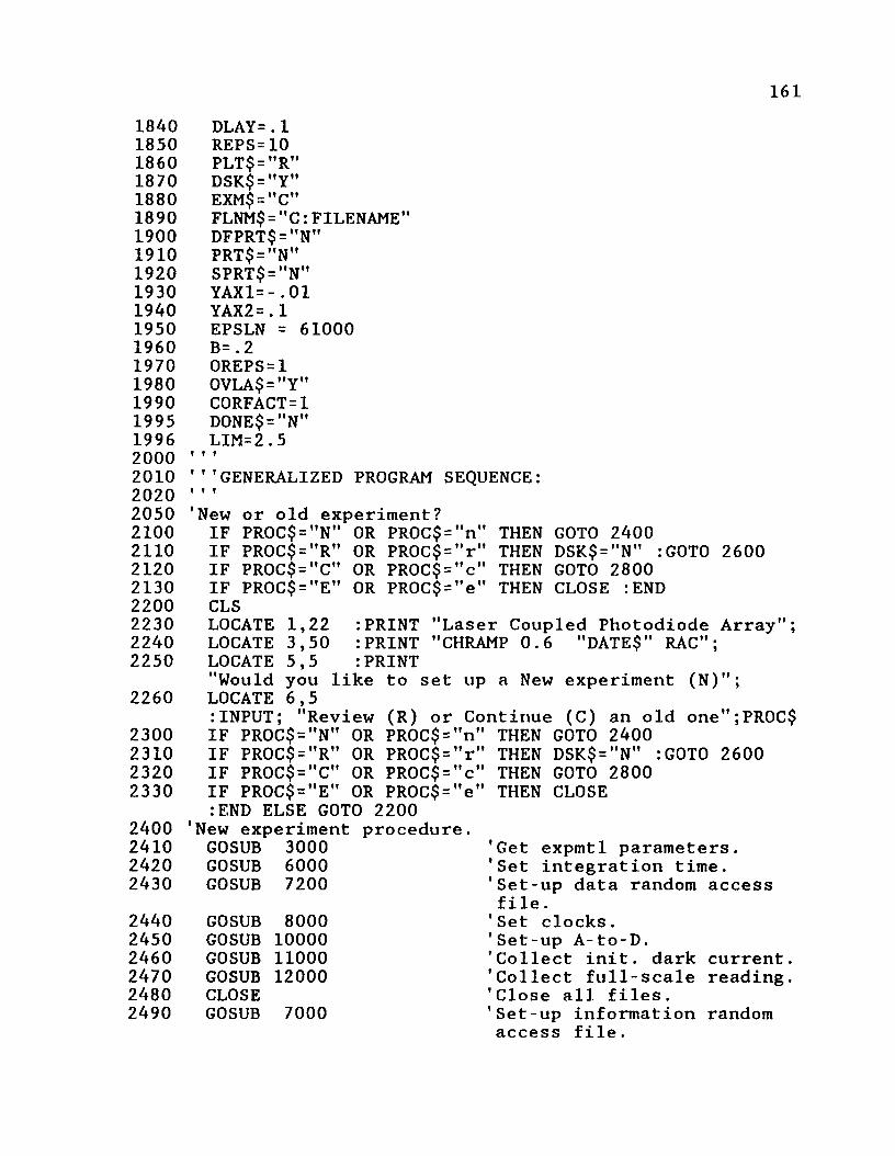
1611840 DLAY=.11850 REPS=101860 PLT$="R"1870 DSK$="Y"1880 EXM$="C"1890 FLNM$="C:FILENAME"1900 DFPRT$="N"1910 PRT$="N"1920 SPRT$="N"1930 YAX1=-.011940 YAX2=.11950 EPSLN = 610001960 B= .21970 OREPS=11980 OVLA$="Y"1990 CORFACT=11995 DONE$="N"1996 LIM=2.52000 f I »

2010 " 'GENERALIZED PROGRAM SEQUENCE:2020 I ? f

2050 'New or old experiment?2100 IF PR0C$="N" OR PR0C$="n" THEN GOTO 24002110 IF PR0C$="R" OR PROC$="r" THEN DSK$="N" :GOTO 26002120 IF PR0C$="C" OR PROC$="c" THEN GOTO 28002130 IF PROC$="E" OR PROC$="e" THEN CLOSE :END2200 CLS2230 LOCATE 1,22 :PRINT "Laser Coupled Photodiode Array";2240 LOCATE 3,50 :PRINT "CHRAMP 0.6 "DATES" RAC";2250 LOCATE 5,5 :PRINT

"Would you like to set up a New experiment (N)";2260 LOCATE 6,5

:INPUT; "Review (R) or Continue (C) an old one";PR0C$2300 IF PR0C$="N" OR PR0C$="n" THEN GOTO 24002310 IF PR0C$="R" OR PR0C$="r" THEN DSK$="N" :GOTO 26002320 IF PR0C$="C" OR PR0C$="c" THEN GOTO 28002330 IF PROC$="E" OR PROC$="e"

:END ELSE GOTO 2200THEN CLOSE

2400 'New experiment procedure.2410 GOSUB 3000 'Get expmtl parameters.2420 GOSUB 6000 'Set integration time.2430 GOSUB 7200 'Set-up data random access

file.2440 GOSUB 8000 'Set clocks.2450 GOSUB 10000 'Set-up A-to-D.2460 GOSUB 11000 'Collect init. dark current.2470 GOSUB 12000 'Collect full-scale reading.2480 CLOSE 'Close all files.2490 GOSUB 7000 'Set-up information random

access file.

1622500 GOSUB 7200

25102520253025402550256025702600261026202630264026502660

2900291029202930294029502960300030103020

GOSUB 14000 GOSUB 11000 GOSUB 26000 GOSUB 15000 CLOSE PROC$="RM GOSUB 17000

'Old experiment GOSUB 20000 GOSUB 3000LOCATE 21,35 GOSUB 3360

procedure

'Re-open data random access f ile.'Collect experimental data. 'Collect final dark current. 'Store & plot current data. 'Data analysis & reduction. 'Closes all open files. 'Switch to review procedure 'New, Review, Cont., or End?

: PRINTGOSUBGOSUB

2630020500

2670 GOSUB 207002680 GOSUB 21000

269027002710280028102820

283028402850286028702880

CLOSEPR0C$=_ "T> "

GOSUB 17000 'Continue experiment.

GOSUB 20000 GOSUB 3000

LOCATE 21,35 :PRINT OREPS=REPS+1 GOSUB 3360 REPS=REPS+OREPS-1GOSUBGOSUB

60007000

2890 GOSUB 7200

GOSUBGOSUBGOSUBGOSUBCLOSEPR0C$=

8000100001400011000

_ " R "GOSUB 17000

EXPERIMENT SET-UP:

'Retrieve parameters.'Print them out (and begin review sequence.)

File name = "FLNM$;'Adjust parameters.'Retieve & plot current data'Retrieve and plot old dark current.'Retrieve and plot old full scale reading.'Retrieve and plot old experimental data.'Close all open files.

'Retrieve parameters. 'Print them out (and begin review sequence.)

File name = "FLNM$;

'Set integration time.'Set up random access information file.'Set up random access data file.'Set clocks.'Set-up A-to-D.'Collect experimental data.'Collect final dark current reading.'Close all open files'Switch to review procedure.'New, Review, Continue, or End?

1633025 'Heading •

3030 CLS :COLOR 7,03040 LOCATE 1,22 :PRINT "Laser Coupled Photodiode Array’3050 LOCATE 2,22 :PRINT " Experimental Set-up";3060 LOCATE 3,50 :PRINT "CHRAMP 0.6 "DATE?" RAC";3070 'Photodiode array parameters.3080 LOCATE 4,2 :PRINT "Photodiode Array -";3090 LOCATE 6,5

:PRINT "Integration time (2.7-333 mSec) =";3100 LOCATE 7,5

:PRINT "Time between sample reads (1-600 Sec) = ";3110 LOCATE 8,5

:PRINT "Number of scans averaged per read =";3120 LOCATE 9,5

:PRINT "Delay between laser pulse and scan read =";3130 LOCATE 10,5 :PRINT "Number of repetitions ="3140 'Data manipulation parameters.3150 LOCATE 12,2 :PRINT "Data Handling3160 LOCATE 14,5

:PRINT "Plot Raw data, Absorbance, Cone., or None?"3165 LOCATE 15,5 :PRINT "Overlay plots?"3170 LOCATE 16,5

:PRINT "Print dark current and full scale plots?"3180 LOCATE 17,5 :PRINT "Print all sample plots?"3190 LOCATE 18,5 :PRINT "Print all raw data out?"3200 LOCATE 19,5 :PRINT "Save data in a disk file?"3205 LOCATE 20,5 :PRINT "Experiment mode?"3206 LOCATE 21,2 :PRINT "Sample info:"3210 'Print default values for each parametre.3220 COLOR 0,7 'Highlight on.3230 LOCATE 6,50 :PRINT " "INTG3240 LOCATE 7,50 :PRINT " "RRAT3250 LOCATE 8,50 :PRINT " "NAVE%3260 LOCATE 9,50 :PRINT " "DLAY3270 LOCATE 10,50 :PRINT " "REPS3280 LOCATE 14,51 :PRINT " "PLT?" "3285 LOCATE 15,51 :PRINT " "OVLA?" "3290 LOCATE 16,51 :PRINT " "DFPRT?" "3300 LOCATE 17,51 :PRINT " "SPRT?" "3310 LOCATE 18,51 :PRINT " "PRT?" "3320 LOCATE 19,51 :PRINT " "DSK?" "3325 LOCATE 20,51 :PRINT " "EXM?" "3326 LOCATE 21,14 :PRINT f t I f

3327 LOCATE 21,14 :PRINT SI?3330 IF PR0C$="R" OR PR0C$="r" THEN COLOR 7,0 :RETURN3340 IF PROC?="C" OR PROC?="c" THEN COLOR 7,0 :RETURN3360 'Procedure to adjust values for individual experiments3370 COLOR 7 , 0 'Highlight off.3380 LOCATE 23,1: PRINT SPACE?(70);3390 LOCATE 24,1: PRINT SPACE?(70);

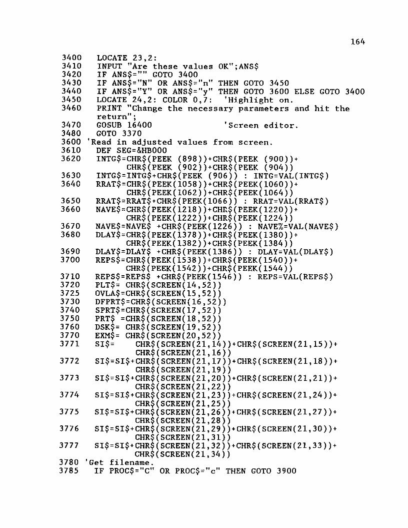
1643400 LOCATE 23,2:3410 INPUT "Are these values OK";ANS$3420 IF ANS$="" GOTO 34003430 IF ANS$="N" OR ANS$="n" THEN GOTO 34503440 IF ANS$="Y" OR ANS$="y" THEN GOTO 3600 ELSE GOTO 34003450 LOCATE 24,2: COLOR 0,7: 'Highlight on.3460 PRINT "Change the necessary parameters and hit the

return";3470 GOSUB 16400 'Screen editor.3480 GOTO 33703600 'Read in adjusted values from screen.3610 DEF SEG=&HB0003620 INTG$ = CHR$(PEEK (898))+CHR$(PEEK (900)) +

CHR$(PEEK (902))+CHR$(PEEK (904))3630 INTG$=INTG$+CHR$(PEEK (906)) : INTG=VAL(INTG$)3640 RRAT$=CHR$(PEEK(1058))+CHR$(PEEK(1060))+

CHR$(PEEK(1062)) + CHR$(PEEK(1064))3650 RRAT$=RRAT$ + CHR$(PEEK(1066)) : RRAT=V A L (RRAT$)3660 NAVE$=CHR$(PEEK(1218))+CHR$(PEEK(1220))+

CHR$(PEEK(1222))+CHR$(PEEK(1224))3670 NAVE$=NAVE$ +CHR$(PEEK(1226)) : NAVE%=VAL(NAVE$)3680 DLAY$=CHR$(PEEK(1378))+CHR$(PEEK(1380))+

CHR$(PEEK(1382))+CHR$(PEEK(1384))3690 DLAY$=DLAY$ +CHR$(PEEK(1386)) : DLAY=V A L (DLAY$)3700 REPS$=CHR$(PEEK(1538))+CHR$(PEEK(1540))+

CHR$(PEEK(1542)) + CHR$(PEEK(1544))3710 REPS$=REPS$ +CHR$(PEEK(1546)) : REPS=VAL(REPS$)3720 PLT$= CHR$(SCREEN(14,52))3725 0VLA$=CHR$(SCREEN(15,52))3730 DFPRT$=CHR$(SCREEN(16,52))3740 SPRT$=CHR$(SCREEN(17,52))3750 PRT$ =CHR$(SCREEN(18,52))3760 DSK$= CHR$(SCREEN(19,52))3770 EXM$= CHR$(SCREEN(20,52))3771 SI$= CHR$(SCREEN(21 14 ) + CHR$(SCREEN(21,15))

CHR$(SCREEN(21 16 )3772 SI$=SI$+CHR$(SCREEN(21 17 )+CHR$(SCREEN(21,18))

CHR$(SCREEN(21 19 )3773 SI$=SI$+CHR$(SCREEN(21 20 ) + CHR$(SCREEN(21,21))CHR$(SCREEN(21 22 )3774 SI$=SI$+CHR$(SCREEN(21 23 ) + CHR$(SCREEN(21,24))CHR$(SCREEN(21 25 )3775 SI$=SI$+CHR$(SCREEN(21 26 )+CHR$(SCREEN(21,27))CHR$(SCREEN(21 28 )3776 SI$=SI$+CHR$(SCREEN(21 29 )+CHR$(SCREEN(21,30))CHR$(SCREEN(21 31 )3777 SI$=SI$+CHR$(SCREEN(21 32 )+CHR$(SCREEN(21,33))CHR$(SCREEN(21 34 )3780 'Get filename.

3785 IF PROC$="C" OR PROC$=' c" THEN GOTO 3900

379038003820383038403850

3860

387039003910392039303940400040104020403040404050406040704080409041004200421042204230

42404250426042654270

42804300

4310

4320

165IF DSK$="Y" OR DSK$="y" THEN GOTO 3800 ELSE GOTO 3900 LOCATE 21,35 :PRINT " File name = C: ";LOCATE 21,50: COLOR 0,7 'Highlight on.GOSUB 16400 'Screen editor.FLNM$= CHR?(SCREEN(21,48))+CHR$(SCREEN(21,49))+

CHR$(SCREEN(21,50))FLNM?= FLNM? + CHR?(SCREEN(21,51)) + CHR?(SCREEN(21,52)) +

CHR?(SCREEN(21,53))FLNM$= FLNM$ + CHR?(S CREEN(21,54))+ CHR?(SCREEN(21,55)) +

CHR$(SCREEN(21,56))FLNM$= FLNM$+CHR$(SCREEN(21,57))

'Get scale for absorbance and concentration plotting.IF PLT?="N" OR PLT$="n" THEN GOTO 4400IF PLT$="R" OR PLT$="r" THEN GOTO 4400IF PLT$="C" OR PLT$="c" THEN GOTO 4000IF PLT$=”A ” OR PLT$="a" THEN GOTO 4200 ELSE GOTO 3360'obtain molar absoptivity, EPSLN, and cell path length, B.

LOCATE 23,1 : PRINT SPACE$(77);LOCATE 24,1 : PRINT SPACE?(77);LOCATE 23,2PRINT "Molar absorptivity =

Cell path = cm";COLOR 0,7LOCATE 23,23 : PRINT " ";LOCATE 23,23 : PRINT EPSLN;LOCATE 23,43 : PRINT " ";LOCATE 23,43 : PRINT BCOLOR 7,0'concentration and absorbance plot scale LOCATE 24,2: PRINT "Plot scale = toCOLOR 0,7LOCATE 24,15: PRINT " " ;:LOCATE 24,24

: PRINT " ";LOCATE 24,15: PRINT YAXl ;:LOCATE 24,24 : PRINT Y A X 2 ; COLOR 7,0GOSUB 16400 'Screen editor.IF PLT$="A" OR PLT$="a" THEN GOTO 4300 EPSLN=VAL(CHR$(SCREEN(23,23))+CHR$(SCREEN(23,24))+

CHR$(SCREEN(23,25))+CHR$(SCREEN(23,26))+CHR$(SCREEN(23,27)) + CHR$(SCREEN(23,28)))

B ='V AL(CHR$(SCREEN(23,43)) + CHR$(SCREEN(23,44)) +CHR$(SCREEN(23,45))+chr$(screen(23,46)))

YAX1=VAL(CHR$(SCREEN(24,15))+CHR$(SCREEN(24,16))+CHR$(SCREEN(24,17)) + CHR$(SCREEN(24,18)) +CHR$(SCREEN(24,19)))

YAX2=VAL(CHR$(SCREEN(24,24))+CHR$(SCREEN(24,25))+CHR$(SCREEN(24,26)) + CHR$(SCREEN(24,27)) +CHR$(SCREEN(24,28)))

AFACT=(-189/(YAX2-YAXl)) : AOFF=189-(AFACT*YAX1)

1664330 EPSLNB=1000/(EPSLN*B) ’Concentration factor.4400 IF PR0C$="R" OR PR0C$="r" THEN GOTO 4700 4500 'Set initial voltage and get final voltage.4505 IF EXM$="C" OR EXM$=”c" THEN GOTO 4510 ELSE GOTO 4700 4510 LOCATE 24,1: PRINT SPACE$(77);4520 LOCATE 23,1: PRINT SPACE$(77);4530 LOCATE 23,2: INPUT "Input intial voltage:",VOLTl4540 DECIMAL=INT(818.8*(V0LT1+.014)): 'add to compensate

for ADC offset 4550 HIGH1=INT(DECIMAL/256): L0W1=DECIMAL-256*HIGH1 4560 IF HIGH1<0 THEN HIGH1=16+HIGH14570 LOCATE 24,2: PRINT "Strike any key to begin applying

potential...";4580 D$=INKEY$:IF D$="" THEN 45804590 OUT ADS1,HIGH1: OUT ADS,L0W14600 LOCATE 24,1: PRINT SPACE$(77);4610 LOCATE 23,1: PRINT SPACE$(77);4620 LOCATE 23,2: INPUT "Input final voltage:",V0LT24630 DECIMAL=INT(818.8*(VOLT2+.014)): 'add to compensate

for DAC offset 4640 HIGH2=INT(DECIMAL/256): LOW2=DECIMAL-256*HIGH24650 IF HIGH2<0 THEN HIGH2=16+HIGH24700 LOCATE 24,1: PRINT SPACE$(77);4710 LOCATE 23,1: PRINT SPACE$(77);4720 LOCATE 23,2:PRINT "Press return to begin experiment"; 4730 LA$=INKEY$

: IF LA$=CHR$(13) THEN GOTO 4740 ELSE GOTO 47304740 LOCATE 23,504750 TM$=LEFT$(TIME$,5)4760 PRINT "Time = "TM$;4770 IF DFPRT$="Y" OR DFPRT$="y" THEN GOSUB 16160 :RETURN4780 IF PRT$="Y" OR PRT$="y" THEN GOSUB 16160 'Hardcopy4790 RETURN 6000 '''6010 ’’'PARALLEL I/O PORT ROUTINE TO SET THE ARRAY

INTEGRATION TIME:6020 ’''6030 'Range for integration time is 0 to 333 msec.

Zero turns it off.6040 MULT=1.5:INTG1=INTG*MULT 'MULT=scan rate/33333,

which is 50000 here.6050 IF INTG1<500 THEN GOTO 61006060 IF INTG1=500 THEN TICKS=0: GOTO 61106070 LOCATE 25,26080 PRINT "Maximum integration time is 333 msec at

50 K H z ."*:6090 GOSUB 16100: GOTO 3450 6100 TICKS=INT((500-INTG1)*8.19)+16110 HI4=INT(TICKS/256) 'Divide into high 4 bits6120 L08=TICKS-HI4*256 'and low 8 bits.

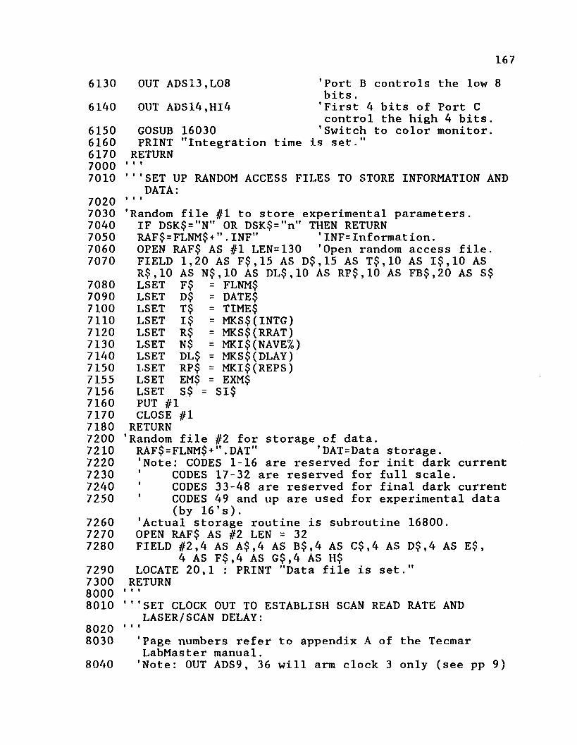
61306140

61506160617070007010702070307040705070607070

7080709071007110712071307140715071557156716071707180720072107220723072407250

726072707280

7290730080008010802080308040

167OUT ADS13,L08 'Port B controls the low 8

bits.OUT ADS14,HI4 'First 4 bits of Port C

GOSUB 16030control the high 4 bits. 'Switch to color monitor.

PRINT "Integration time is set. RETURN’’’SET UP RANDOM ACCESS FILES TO STORE INFORMATION AND

DATA:'Random file #1 to store experimental parameters.

IF DSK?="N" OR DSK?="n" THEN RETURN RAF?=FLNM?+".INF" ’INF=Information.OPEN RAF? AS #1 LEN=130 'Open random access file. FIELD 1,20 AS F? , 15 AS D? , 15 AS T ? ,10 AS I?, 10 AS R $ ,10 AS N $ ,10 AS D L $ ,10 AS RP?,10 AS FB?,20 AS S$ LSET F? = FLNM?LSET D? = DATE?LSET T? = TIME?LSET I? = MKS?(INTG)LSET R? = MKS?(RRAT)LSET N? = MKI?(NAVE%)LSET DL? = MKS?(DLAY)LSET RP? = MKI?(REPS)LSET EM? = EXM?LSET S? = SI?PUT #1 CLOSE #1

RETURN'Random file #2 for storage of data.

RAF?=FLNM?+".DAT" 'DAT=Data storage.'Note: CODES 1-16 are reserved for init dark current ' CODES 17-32 are reserved for full scale.' CODES 33-48 are reserved for final dark current' CODES 49 and up are used for experimental data

(by 16's ).'Actual storage routine is subroutine 16800.OPEN RAF? AS #2 LEN = 3 2FIELD #2,4 AS A?,4 AS B?,4 AS C?,4 AS D?,4 AS E ? ,

4 AS F ? ,4 AS G ? ,4 AS H?LOCATE 20,1 : PRINT "Data file is set."

RETURN'''SET CLOCK OUT TO ESTABLISH SCAN READ RATE AND

LASER/SCAN DELAY:'Page numbers refer to appendix A of the Tecmar LabMaster manual.'Note: OUT ADS9, 36 will arm clock 3 only (see pp 9)

1688050806080708080

80908100811081208130814081508160

8170

818081908200

8210

82158220

8240826082708280

82908300831083208330834083508360

OUT ADS9

OUT ADS9, 220

'Clock 3 is used OUT ADS9,23:

as

OUT A D S 9 , 40 will arm clock 4 only(to read the dark current)56 will arm both clocks 4 and 5 to pulse the laser followed by reading the photodiode array.

'Disarm counters 3,4, and 5. (ppl4)

the master clock.'Set data pointer to MM register.'BCD count, etc.(see pp 23 of appendix)

'Set data pointer to counter mode of clock 3,

fig. 3 and pp 23, fig 4). 'Set clock 3 up for no gating, count rising

'edge, bed count, count down, etc. (pp 24 Fig 7) 'Count rate is set so that 100 counts=l sec. The range is .01 to 640 sec

CNTDWN =200*RRAT-0 'Calculate decimalcountdown number.

CNTDWN$=MID$(STR$(CNTDWN),2)HEXRATE=VAL("&H"+CNTDWN$) 'Conversion to hex.

OUT A D S 8 ,0:OUT A D S 8 ,128: OUT ADS9,3

'(PP 14, OUT A D S 8 ,49:OUT A D S 8 ,15

MSB=INT(HEXRATE/256)

LSB=INT(HEXRATE- 256 *MSB)'Divide into most significant byte 'and least significant b y t e .

'print "msb="msb " lsb="lsb OUT ADS8,LSB:OUT ADS8,MSB 'Load

load ' Load

for laser pulsing.'Set data pointer to MM

OUT A D S 9 ,68 'Set up clock 5

OUT ADS9,23:

counter of register, counter 3.

clock 3

(PP 9)

OUT A D S 8 ,0:OUT A D S 8 ,128

OUT ADS9,5OUT A D S 8 ,17:OUT ADS8,11

'bed osc

LSB=INT(2):MSB=INT(0)OUT ADS8,LSB: OUT ADS8,MSB

register,'BCD count, etc. (see pp 23 of appendix)'Set data pointer to counter mode of clock 4, 'Set clock 5 up for no gating, count once,

count, count down, freq., etc. (pp 24 Fig 7)

OUT ADS9,80 'Set up clock 4 OUT ADS9,23:

'Load clock 5 load register with 2 (min.) 'Load counter 5. (pp 9)

for reading the diode array.'Set data pointer to MM register.

169'BCD count, etc. (see pp 23 of appendix)'Set data pointer to counter mode of clock 4. 'Set clock 4 like clock 5. 'Calculate decimal countdown.

8410 CNTDWN?=MID?(STR?(CNTDWN),2)8420 HEXRATE=VAL("&H"+CNTDWN?)8430 MSB=INT(HEXRATE/256)8440 LSB=INT(HEXRATE-256*MSB)

8450 OUT ADS8 ,LSB:0UT ADS8,MSB

8460 OUT ADS9,728470 PRINT "Clocks are set."8480 RETURN 10000 '’’10010 '''ANALOG-TO-DIGITAL CONVERTER SET UP AND DATA

COLLECTION:10020 ' ' '

10030 'This routine collects 128 data points per scan A/D channel #0.

10035 'This line has no tabs.10040 'Initialize ADC. Program line 1240 disables

external start conversions.10050 OUT ADS4,132 'Enable ext start conv.,

disable auto-inc.10060 OUT ADS5,0 'Write channel number to

board.10070 PRINT "A-to-D converter is set."10080 RETURN11000 '''Dark current collection, initial and final.11010 FOR I%=1 TO 128:SAM(I%)=0:NEXT 11020 IF D0NE?="Y" THEN GOTO 11065 11030 LOCATE 12,1 11040 PRINT "Hit return";11050 LOCATE 13,111060 INPUT "when ready.",ANS?11061 CLS11065 FOR H %=1 TO 9 11070 FOR 1% = 1 TO NAVE7o11080 OUT ADS9,40 'Pulse scan sequencer ONLY.11090 CALL A D C (DATAREA%) 'Read array. ADC is an

assembler call in SLAVE. 11100 DEF SEG=DATAREA% 'DATAREA% is where the

data is stored.11110 FOR J7o=2 TO 256 STEP 211120 SAM(J%/2)=SAM(J%/2)+(256*PEEK(J%+l)+PEEK(J%))

'Convert to hex.'Divide into Most Significant Byte and 'Least Significant B y t e .'Load counter of clock 4 load register.

'Load counter 4. (pp 9)

8370 OUT A D S 8 ,0:OUT A D S 8 ,128:

8380 OUT A D S 9 ,48390 OUT A D S 8 ,17:OUT ADS8,118400 CNTDWN =1000*DLAY-0

17011130 NEXT J7a11200 NEXT I%11205 NEXT H%11210 FOR I%=1 TO 12811220 SAM(I%) = SAM(I/£)/(NAVE%*9)11230 IF DONE$="Y" THEN FDRK(I7) = SAM(I70)

ELSE IDRK(I%)= SAM(I%)11240 NEXT 17o11250 'Store, plot, and print dark current data.11260 CLS11270 IF D0NE$="Y" THEN GOTO 11280 ELSE GOTO 1130011280 LOCATE 2,4: PRINT "Final";: GOTO 1131011300 LOCATE 2,3: PRINT "Initial";11310 LOCATE 3,1: PRINT "Dark Current";11320 GOSUB 18120 'Plot raw data.11330 IF D0NE$="Y" THEN GOTO 1141011340 LOCATE 23,1: INPUT"Is this 0K";ANS$11350 IF ANS$="N" OR ANS$="n" THEN GOTO 11000 11360 LOCATE 23,1: PRINT SPACE$(14);11370 IF PRT$="Y" OR PRT$="y" THEN GOSUB 18000 11380 IF DFPRT$="Y" OR DFPRT$="y" THEN GOSUB 1616011390 IF DSK$ ="Y" OR DSK$ ="y" THEN CODE=l: GOSUB 1680011400 RETURN11410 'Initial/Final dark current comparison.11420 LODIF=FDRK(1)-IDRK(1): HIDIF=LODIF11430 FOR 1% = 1 TO 12811440 DIF=FDRK(1%)-IDRK(1%)11450 IF DIF<LODIF THEN LODIF=DIF11460 IF DIF>HIDIF THEN HIDIF=DIF11470 NEXT 1%11480 LOCATE 22,2: PRINT "Difference";11490 LOCATE 23,2: PRINT " range =";11500 LOCATE 24,1: PRINT LODIF" to "HIDIF;11510 IF DFPRT$="Y" OR DFPRT$="y" THEN GOSUB 1616011520 IF DSK$ ="Y" OR DSK$ ="y" THEN CODE=33: GOSUB 16800 11530 LOCATE 25,2 : INPUT "O.K.",ANS$11540 RETURN12000 '''INITIAL full scale reading.12001 input "wait";w12010 LOCATE 12,1: PRINT "Hit return";12020 LOCATE 13,1: INPUT "when ready.",ANS$12070 CLS12080 OUT A D S 9 ,220 'Disable master clock (#3)

and clocks 4 and 5.12090 OUT ADS9,36 'Enable master clock (#3).12100 FOR H7=l TO NAVE%+112110 OUT ADS9,164 'Save counter 3 in its hold

register.12120 IF INP(ADS8)=1 AND INP(ADS8)=0 THEN GOTO 12200 ELSE

GOTO 12110

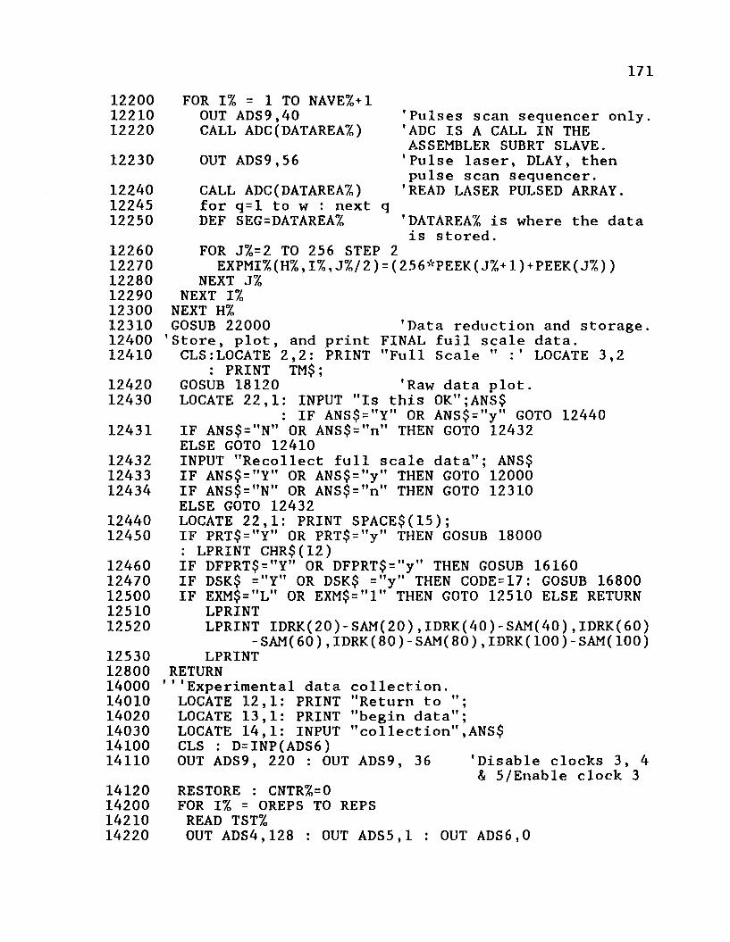
17112200122101222012230

122401224512250

12260122701228012290123001231012400124101242012430

124311243212433124341244012450

1246012470125001251012520125301280014000140101402014030141001411014120142001421014220

FOR 1% = 1 TO NAVE7+1 OUT ADS9,40 CALL A D C (DATAREA7)OUT ADS9,56

CALL ADC(DATAREA7o) for q=l to w : next DEF SEG=DATAREA7o

'Pulses scan sequencer only 'ADC IS A CALL IN THE ASSEMBLER SUBRT SLAVE. 'Pulse laser, DLAY, then pulse scan sequencer.'READ LASER PULSED ARRAY.

'DATAREA7 is where the data is stored.

FOR J%=2 TO 256 STEP 2EXPMI7o(H % , 1%, J7o/ 2 ) = (256*PEEK (J7o+1) + PEEK( J7„))

NEXT J%NEXT IZ

NEXT H ZGOSUB 22000 'Data reduction and storage.'Store, plot, and print FINAL full scale data.

C L S :LOCATE 2,2: PRINT "Full Scale " LOCATE 3,2: PRINT T M $ ;

GOSUB 18120 'Raw data plot.LOCATE 22,1: INPUT "Is this 0K";ANS$

: IF ANS$="Y" OR ANS$="y" GOTO 12440 IF ANS$="N" OR ANS$="n" THEN GOTO 12432 ELSE GOTO 12410INPUT "Recollect full scale data"; ANS$IF ANS$="Y" OR ANS$="y" THEN GOTO 12000IF ANS$="N" OR ANS$="n" THEN GOTO 12310ELSE GOTO 12432LOCATE 22,1: PRINT SPACE$(15);IF PRT$="Y" OR PRT$="y" THEN GOSUB 18000 : LPRINT CHR$(12)IF DFPRT$="Y" OR DFPRT$="y" THEN GOSUB 16160 IF DSK$ ="Y" OR DSK$ ="y" THEN CODE=17: GOSUB 16800IF EXM$="L" OR EXM$="1" THEN GOTO 12510 ELSE RETURN

LPRINTLPRINT IDRK(20)-SAM(20),IDRK(40)-SAM(40),IDRK(60)

-SAM(60),IDRK(80)-SAM(80),IDRK(100)-SAM(100) LPRINT

RETURN'''Experimental data collection.

LOCATE 12,1: PRINT "Return to LOCATE 13,1: PRINT "begin data";LOCATE 14,1: INPUT "collection",ANS$CLS : D=INP(ADS6)OUT ADS9, 220 : OUT ADS9, 36RESTORE : CNTR%=0 FOR IZ = OREPS TO REPS READ TST%OUT A D S 4 ,128 : OUT ADS5.1

'Disable clocks 3, & 5/Enable clock

OUT ADS6,0

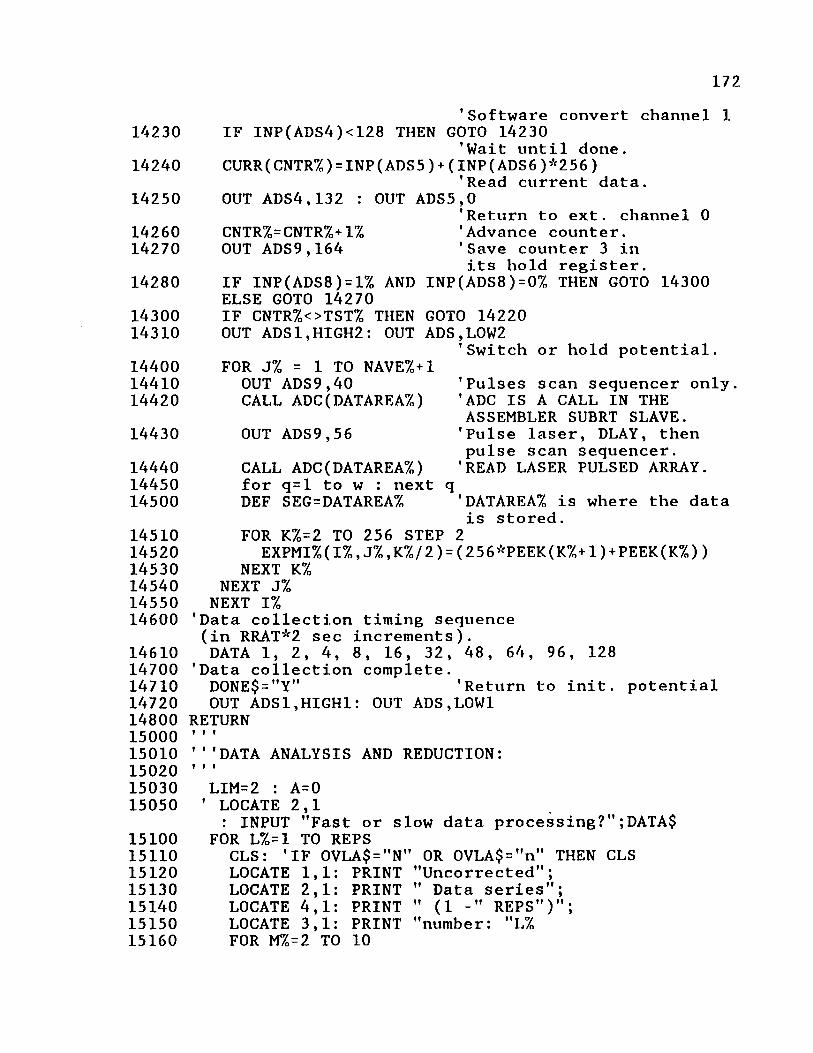
172

142301424014250142601427014280

1430014310

14400144101442014430

14440144501450014510145201453014540145501460014610147001471014720148001500015010150201503015050

15100151101512015130151401515015160

'Software convert channel 1 IF INP(ADS4)<128 THEN GOTO 14230

'Wait until done.CURR(CNTR7) = INP(ADS 5) + (INP(ADS 6)*2 5 6)

'Read current data.OUT A D S 4 ,132 : OUT ADS5,0

'Return to ext. channel 0 CNTR%= CNTR%+1% 'Advance counter.OUT ADS9,164 'Save counter 3 in

its hold register.IF INP(ADS8)=1% AND INP(A DS8)=0% THEN GOTO 14300 ELSE GOTO 14270IF CNTR%<>TST% THEN GOTO 14220 OUT ADSl,HIGH2: OUT ADS,LOW2

'Switch or hold potential.FOR J% = 1 TO NAVE7o+l

OUT ADS9,40 CALL A D C (DATAREA7)OUT ADS9,56

CALL A D C (DATAREA7) for q=l to w : next DEF SEG = DATAREA7

'Pulses scan sequencer only, 'ADC IS A CALL IN THE ASSEMBLER SUBRT SLAVE. 'Pulse laser, DLAY, then pulse scan sequencer.'READ LASER PULSED ARRAY.

'DATAREA7 is where the data is stored.

FOR K%=2 TO 256 STEP 2EXPMI% (1%, J7o, K 7 / 2 ) = (2 5 6 *PEEK (K7o+1) + PEEK ( K7o))

NEXT K7o NEXT J%

NEXT I%'Data collection timing sequence (in RRAT*2 sec increments).DATA 1, 2, 4, 8, 16, 32, 48, 64, 96, 128

'Data collection complete.D0NE$="Y" 'Return to init. potentialOUT ADSl,HIGH1: OUT ADS,L0W1

RETURN'''DATA ANALYSIS AND REDUCTION:f f f

LIM=2 : A=0 LOCATE 2,1: INPUT "Fast or slow data processing?";DATA$

FOR L%=1 TO REPSCLS: 'IF OVLA$="N" OR 0VLA$="n" THEN CLSLOCATE 1,1 LOCATE 2,1 LOCATE 4,1 LOCATE 3,1

PRINT "Uncorrected"; PRINT " Data series"; PRINT " (1 REPS")" PRINT "number: "L7o

FOR M7=2 TO 10

15170 FOR I%=1 TO 12815200 SAM(I%) = EXPMI7o(L%,M7o,I%)15210 EXPM(M7o,l7o) = EXPMI7o(L7o,M%,I7o)15220 NEXT 1%15230 IF PLT$="R" OR PLT$="r" THEN GOSUB 1812015240 IF PLT$="C" OR PLT$="c" THEN GOSUB 1870015250 IF PLT$="A" OR PLT$="a" THEN GOSUB 1840015260 IF SPRT$="Y" OR SPRT$="y" THEN GOSUB 16160

'Hardcopy.15270 IF PRT$="Y" OR PRT$="y" THEN GOSUB 1800015300 NEXT M7o15310 CLS15313 LOCATE 1,1

: INPUT "Should the data be normalized?";NORM$15314 IF NORM$="A" OR NORM$="a" THEN GOTO 1531715315 IF NORM$="Y" OR NORM$="y" THEN GOTO 1532515316 IF NORM$="N" OR NORM$="n" THEN GOTO 15470

ELSE GOTO 1531315317 FOR M7=2 TO 1015318 FOR I%=1 TO 12815219 SAM(I%) = EXPMI7(L 7 ,M % ,1%)15320 NEXT 1%15321 D=L%+M%-2: CODE=80+D*20: GOSUB 1680015322 NEXT M%15323 A = 10: GOTO 1552015325 FOR m = 2 TO 1015330 GOSUB 24000 'Correction factor.15340 ' CLS15350 LOCATE 1,1: PRINT " Normalized";15360 LOCATE 2,1: PRINT " Data series";15370 LOCATE 4,1: PRINT " (1 REPS")";15400 LOCATE 3,1: PRINT "number: "L%15410 IF PLT$="R" OR PLT$="r" THEN GOSUB 1812015420 IF PLT$="C" OR PLT$="c" THEN GOSUB 1870015430 IF PLT$="A" OR PLT$="a" THEN GOSUB 1840015440 IF SPRT$="Y" OR SPRT$="y" THEN GOSUB 16160

'Hardcopy.15450 IF PRT$="Y" OR PRT$="y" THEN GOSUB 1800015460 NEXT M%15470 GOSUB 24100 'Statistical Analysis.15500 'Data Storage.15505 D=L%+A15510 IF DSK$="Y" OR DSK$="y" THEN CODE=80+D*20

: GOSUB 16800 15520 NEXT L%15530 RETURN 16000 '''16010 ''’MISCELLANEOUS SUBROUTINES:16020 '''16030 'Switch to color screen.

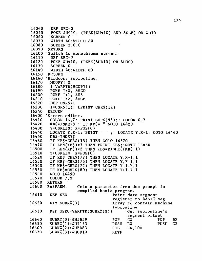
174160401605016060160701608016090161001611016120161301614016150161601617016180161901620016210162201623016240164001641016420164301644016450164601647016500165101652016530165401655016560165701658016600

(PEEK(&H410) AND &HCF) OR &H1080

screen.

DEF SEG=0 POKE &H410,SCREEN 0 WIDTH 40:WIDTH SCREEN 2,0,0

RETURN'Switch to monochrome

DEF SEG=0POKE &H410, (PEEK(&H410) OR &H30)SCREEN 0WIDTH 40:WIDTH 80

RETURN'Hardcopy subroutine.H COPY!=0 I=VARPTR(H C O P Y !)POKE 1 + 0, &HCD POKE 1 + 1, &H5 POKE 1+2, &HCB DEF USR5=II=USR5(I ): LPRINT CHR$(12)

RETURN'Screen editor.

COLOR 16,7: PRINT KB$=INKEY$ : IF KB$=""Y=CSRLIN: X=P0S(0)LOCATE Y,X-1: PRINT KB$=INKEY$IF KB$=CHR$(13) THEN GOTO 16570 IF LEN(KB$)=1 THEN PRINT KB$;:GOTO 16450 IF LEN(KB$)=2 THEN KB$=RIGHT$(KB$,1) Y=CSRLIN: X=POS(0)IF KB$=CHR$(77) THEN IF KB$=CHR$(75) THEN IF KB$=CHR$(72) THEN IF KB$=CHR$(80) THEN GOTO 16450 COLOR 7,0

RETURN 'BASPARM:

CHR$(95); GOTO

COLOR16420

0,7

LOCATE Y ,X- 1: GOTO 16460

LOCATELOCATELOCATELOCATE

Y ,X + 1,1 Y ,X - 1,1 Y - 1 ,X,1 Y+1,X , 1

16610 DEF SEG16620 DIM SUBR%(3)

Gets a parameter from dos prompt in compiled basic program.

'Point data segment register to BASIC seg'Array to contain machine subroutine

16630 DEF USR0=VARPTR(SUBR%(0))

16640 SUBR%(0)=&H5B5916650 SUBR%(1)=&H5153 16660 SUBR%(2) = &HEB8 316670 SUBR%(3) = &HCB10

'POP 'PUSH 'SUB ' RETF

Get subroutine's segment offset CX POPBX PUSHBX,10H

BXCX

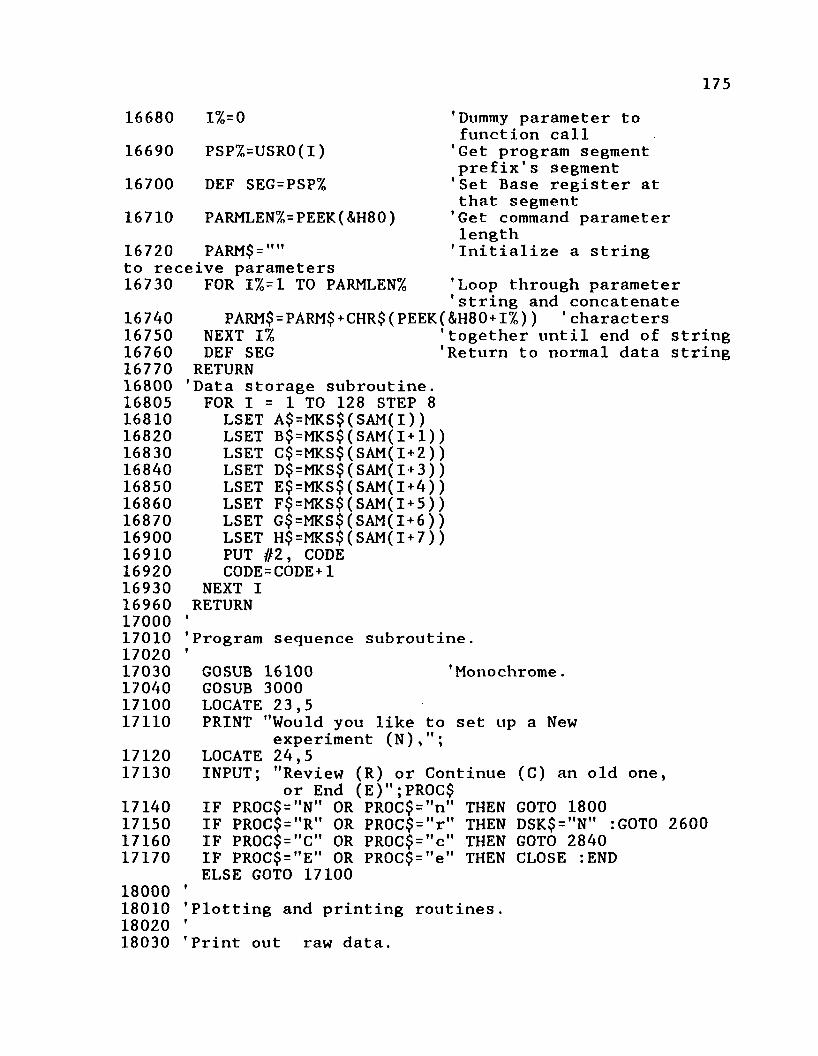
17516680 I%=016690 PSP7o=USR0(I)16700 DEF SEG=PSP%16710 PARMLEN%=PEEK(&H80)16720 to re 16730

16740167501676016770168001680516810168201683016840168501686016870169001691016920169301696017000170101702017030170401710017110

1712017130

17140171501716017170

18000180101802018030

PARM$="" ceive parameters

FOR I%=1 TO PARMLEN%

’Dummy parameter to function call 'Get program segment prefix's segment 'Set Base register at that segment 'Get command parameter length 'Initialize a string'Loop through parameter 'string and concatenate

PARM$=PARM$+CHR$(PEEK(&H80+1%)) 'charactersNEXT I%DEF SEG

RETURN'Data storage subroutine.

FOR I = 1 TO 128 STEP 8 LSET A$=MKS$(SAM(I)) LSET B$=MKS$(SAM(I+1) LSET C$=MKS$(SAM(1+2) LSET D$=MKS$(SAM(I+3) LSET E$=MKS$(SAM(I+4) LSET F$=MKS$(SAM(I+5) LSET G$=MKS$(SAM(I+6) LSET H$=MKS$(SAM(1 + 7) PUT #2, CODE CODE=CODE+1

NEXT I RETURN'Program sequence subroutine.

'together until end of string 'Return to normal data string

GOSUB 16100 'Monochrome.GOSUB 3000 LOCATE 23,5PRINT "Would you like to set up a New

experiment (N),";LOCATE 24,5INPUT; "Review (R) or Continue (C) an old one,

or End (E)";PR0C$IF PR0C$="N" OR PR0C$="n" THEN GOTO 1800IF PR0C$="R" OR PR0C$="r" THEN DSK$="N" :G0T0 2600IF PR0C$="C" OR PR0C$="c" THEN GOTO 2840IF PR0C$="E" OR PROC$="e" THEN CLOSE :ENDELSE GOTO 17100f

'Plotting and printing routines.»

'Print out raw data.

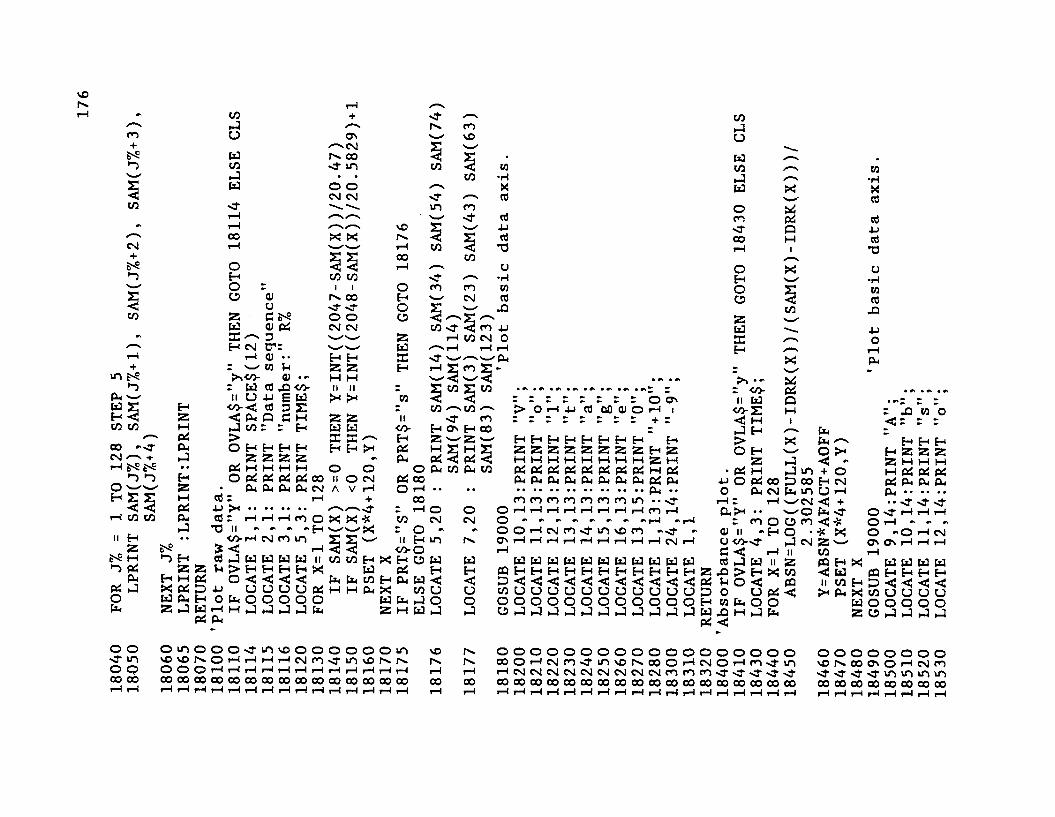
SOrX

#s CO + xt/*—S /--V rx mm u Os w vO+ ^ C M v >—ss w oo ^ y a•-> CO -J- in CO < 03

•J • • co •H5

w o oCM CM

s—V03

C/3 «£■ ■— m m/— \ /—s w c3

•> r-^ ---V/--S SO 2 x / X00 X X rx. <; y cS

CM r-l rH CO < T3+ y* y* 00 COS'S o iX / X O•") Ex CO CO <j- --N •H

O r 1 1 O m m 03£ O 0) rx oo Ex X-' CM c3O -o <r O y x_ X i

CO Z CSS o o CJ ^ ^ £ ^xW a) pi CM CM co sO < m X»■ X_XN_^ z iX CO CM o/—' H cm err w '-"x |-X iX iX

tX iX <v • • Ex H ac %a- >— — ■ pj+ r w oj X Z Z Ex rX y m £ -

m ?-s >~,v> ai • - H H X—✓ v / *"3 r W cfl J3 co­ II II z £ co £ co

ex >— il L3 4J £ ed >H >X 03W £ H <o- < cj 3 s - CO COEx < j z •< ex q c h Z Z II -O mC/3 CO H J c o : : Ex w w co- Ex Os Ex 00

■—' Pi > ffi 33 ^ Ex Z W S X_HOO '■'3’ ex O Ex H Ex Ex Ex Ex >x Pi M £ H £CM + Z Z Z Z * ex eii <q pci <2•x1 £-■? £>>6 e»i H M H H o o o ex co ex co

*-3 *-3 H O Pi Pi Pi Pi 00 II O CM Pi 00O w w z ex ex ex p< cm A V i“ 1 O rX • • • a

CO CO

ii H Z

S'S H •-> Pi

(X, Pi Jof x

p i(X►J

S'S•")

HXwz

ceXIa)

T3

5c3ViX)O

- iX ?X t—I fOII - a - H$ 1 2 3 m< 1—(_J W W to w II> Ex Ex ExH XO < < < <u u u u Pifc o o o o oM J -3 hJ ►J(X

r— I +

O X X *^xco co H

Wfx Px C/3 tX H P-t

00 0 iX C/3r O ii H <0-0 H O PiCX W

co Px XI H W

r r r r r r r r o o s> O H X I C S M O ) O H Ir r r r r r r r + r

H H H H H H H H * H Z Z Z Z Z Z Z Z E x zM H H M H M M M Z Mp i P i p i p i P i P i p i P i l - X C XevexevevevcL.exexpiev • • •• • • • • • • • * • • • • • •

m m m m m m m mO o O *x iX iX iX iX iX iX iX m rXCM CM o - - #s - - fX iX

#s »> o o r-l CM m -d- msom #s<r #>m Os iX T—1?X iX rX iX tXtX -1 CM I-1

iXw w wwWWWwu WWUwH H eo Ex HHHH HH Ex H Ex H■< C D < CC < < C< *<<! -< <U U CO U U o U O u U UUOOo O o o o o o Oo o OOOo►J cJ O J •J hJhJJ J J J J J

C/3*1U

wC/3■Jw

om<rCO

OHOO

ZWaeExX •»

r ■co­il w

« - S C M J Ex >O H

Z• Pi M

x O X 00 o ex cm

H I rH CXpx ..r m o

a/ ii - h o < /> < rc <

X

5Pio

c/3

a) 2 ; . o Pi Vi D O Ex w W jOX <!

XPia

Jj m D oo (X m wcMw o O m O

OCM

CM

Px Cx O <+H U < + fx <r xC-5s * X Z C/3 PQ C ii

px

03• r l*rtcdXIcO

*0

u•H03cC

J3

XO

iXCX

r jo a o < z z z

Ex Ex H Ex Z Z Z Z tx H IX H Pi Pi Xptj ex ex ex

• • • • « ••• xf <r <rO ' ? X H X O r-4 • * • * * *O *» O CSjO' ON H r l Hr —1X u u w wCQ Ex Ex Ex ExH D «< C < C

x w u u o u w o o o o oZ O J *J _3 J

oo omoooMtmvooooooom soMT SO l O v O N O H r l r l H M d ' J i f U D I ' s S N- f ' *O O O O O r l H r l r l r l r l r l r l r l H r l r l i—I rX00 00 OOOOOOOOOOOOOOOOOOOOCOCOCOOOGO 00 00*X iX iX r—I r-X tX r-X T-X fX I-X f-X I-X T-X tX i—I fX (X iX |X

o o o o o o o o o o o o o o o o o oo o o H N n > f i n \ o N o o O r i N O H n ^ i nH c M N M C M N N N N C M n t n t n s f ' J ' J ' J M ’o o o o o o o o o o o o o o o o o o o o o o o o o o o o o o o o o o o oH r l i X i X r l r l H H H H H r l r l i X H H i X r l

o o o o o o o ov O N O O O i O H N mooo o o oo o o oo o o oo o

17718540 LOCATE 13,14:PRINT "r” ;18550 LOCATE 14,14:PRINT "b";18560 LOCATE 15,14:PRINT "a” ;18570 LOCATE 16,14:PRINT "n";18580 LOCATE 17,14:PRINT "c";18590 LOCATE 18,14:PRINT "e";18600 'LOCATE 13,15:PRINT YAX2/2 18610 LOCATE 1,11 :PRINT Y AX2;18620 LOCATE 24,11-.PRINT YAXl;18630 LOCATE 1,118640 RETURN18700 'Concentration plot.18710 IF OVLA$="Y" OR OVLA$="y" THEN GOTO 18730 ELSE CLS 18730 LOCATE 4,3: PRINT TIME$;18735 'LOCATE 6,1:PRINT EPSLN18740 FOR X=1 TO 12818750 ABSN=LOG((FULL(X)-IDRK(X))/(SAM(X)-IDRK(X)))/

2.302585 18760 Y=ABSN*(EPSLNB)

18770 Y =Y*AFACT+AOFF18780 PSET (X*4+120,Y )18800 NEXT X18810 GOSUB 1900018820 LOCATE 7,14 :PRINT "C"18830 LOCATE 8,14 :PRINT "o"18840 LOCATE 9,14 :PRINT "n"18850 LOCATE 10,14:PRINT "c"18860 LOCATE 11,14:PRINT "e"18870 LOCATE 12,14:PRINT "n"18880 LOCATE 13,14:PRINT "t"18890 LOCATE 14,14:PRINT "r"18900 LOCATE 15,14:PRINT "a"18910 LOCATE 16,14:PRINT "t"18920 LOCATE 17,14:PRINT "i"18930 LOCATE 18,14:PRINT "o"18940 LOCATE 19,14:PRINT "n"18941 LOCATE 21,13:PRINT "mM18950 LOCATE 24,11:PRINT YAXl;18970 LOCATE 1,11:PRINT Y A X 2 ;18980 LOCATE 1,118990 RETURN19000 'Basic axis plotting subroutine.19010 FOR X=632 TO 120 STEP -3219020 LINE (X,188)-(X,190) 'X-AXIS TICK MARKS19030 NEXT X19040 FOR Y=190 TO 0 STEP -1919050 LINE (120,Y )-(122,Y ) 'Y-AXIS TICK MARKS19060 NEXT Y19070 PRESET (120,0)

'A=ebc; c=A/eb; epslnb=1000/(epsln*b) 'Scale to fit graphics 'display.'Plot basic data axis.

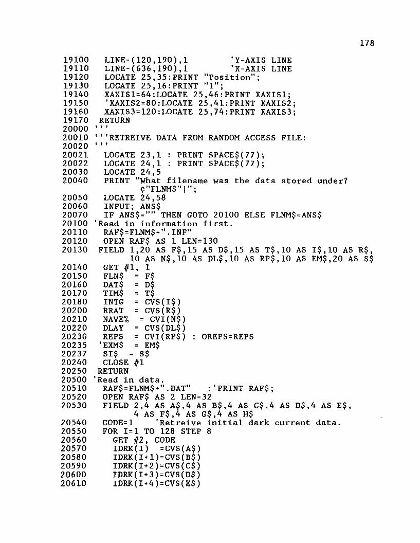
17819100 LINE-(120,190),1 ’Y-AXIS LINE19110 LINE-(636,190),1 'X-AXIS LINE19120 LOCATE 25,35:PRINT "Position” ;19130 LOCATE 25,16:PRINT "1";19140 XAXIS1=64:LOCATE 25,46:PRINT XAXIS1;19150 'XAXIS2=80:LOCATE 25.41:PRINT XAXIS2;19160 XAXIS3 = 120-.LOCATE 25,74: PRINT XAXIS3 ;19170 RETURN20000 ’'’20010 '''RETREIVE DATA FROM RANDOM ACCESS FILE:20020 '''20021 LOCATE 23,1 : PRINT SPACE$(77);20022 LOCATE 24,1 : PRINT SPACE$(77);20030 LOCATE 24,520040 PRINT "What filename was the data stored under?

<?"FLNM$"| ";20050 LOCATE 24,5820060 INPUT; ANS$20070 IF ANS$="" THEN GOTO 20100 ELSE FLNM$=ANS$20100 'Read in information first.20110 RAF$=FLNM$+".INF"20120 OPEN RAF$ AS 1 LEN=13020130 FIELD 1,20 AS F$,15 AS D $ ,15 AS T $ ,10 AS I$,10 AS R $ ,

10 AS N $ ,10 AS D L $ ,10 AS RP$,10 AS EM$,20 AS S$20140 GET #1, 120150 FLN$ = F$20160 DAT$ = D$20170 TIM$ = T$20180 INTG = CVS(I$)20200 RRAT = CVS(R$)20210 NAVE% = CVI(N$)20220 DLAY = CVS(DL$)20230 REPS = CVI(RP$) : OREPS=REPS20235 'EXM$ = EM$20237 SI$ = S$20240 CLOSE #120250 RETURN20500 'Read in data.20510 RAF$=FLNM$+".DAT" :'PRINT RAF$;20520 OPEN RAF$ AS 2 LEN=3220530 FIELD 2,4 AS A$,4 AS B$,4 AS C$,4 AS D$,4 AS E $ ,

4 AS F $ ,4 AS G $ ,4 AS H$20540 CODE=l 'Retreive initial dark current data.20550 FOR 1=1 TO 128 STEP 820560 GET #2, CODE20570 IDRK(I) =CVS(A$)20580 IDRK(1+1)=CVS(B$)20590 IDRK(1+2)=CVS(C$)20600 IDRK(I+3)=CVS(D$)20610 IDRK(I+4)=CVS(E$)

20620206302064020650206602067020671206752068020682206902070020710207202073020740207502076020770208002081020820208302084020850208602086520870208802088120882208902100021005210102102021030210502106021100211102112021130211402115021160211702120021210

179IDRK(I+5)=CVS(F?)IDRK(1+6)=CVS(G$)IDRK(I+7)=CVS(H$)CODE=CODE+1

NEXT IFOR 1=1 TO 128: SAM(I)=IDRK(I): NEXT

’ LOCATE 23,1: PRINT SPACE?(77);' LOCATE 23,2

: INPUT "Hit return to view dark current. " ,ANS$ GOSUB 16030: GOSUB 18120 ’Plot dark current.IF PRT$="Y" OR PRT$ = ’’y" THEN GOSUB 18000

RETURNCODE=17 'Retreive full scale data.FOR 1=1 TO 128 STEP 8

GET #2, CODE FULL(I ) =CVS(A$)FULL(1+1)=CVS(B$)FULL(1+2)=CVS(C $ )FULL(I+3)=CVS(D$)FULL(I+4)=CVS(E?)FULL(I+5)=CVS(F$)FULL(I+6)=CVS(G$)FULL(I+7)=CVS(H$)CODE=CODE+1

NEXT IFOR 1 = 1 TO 128: SAM(I )= FULL(I ): NEXT LOCATE 12,1: PRINT ” Hit return";LOCATE 13,1: PRINT " to view ";LOCATE 14,1: INPUT " full scale.",ANS$GOSUB 18120 'Plot full scale.IF DFPRT$="Y" OR DFPRT$="y" THEN GOSUB 16160 IF PRT$="Y" OR PRT$="y" THEN GOSUB 18000

RETURN'Retreive experimental data.LOCATE 2,1: INPUT "Continue";ANS$ :CLS LOCATE 2,1: PRINT "Data sequence";LOCATE 4,1: PRINT " (1 REPS")";LOCATE 3,1: INPUT "number: ",1%CODE=80+I%*20 IF CODE=80 GOTO 21370 FOR I%=1 TO 128 STEP 8

GET #2, CODE SAM(I%) =CVS(A$)SAM(I%+1)=CVS(B$)SAM(l7o+2) = CVS(C$)SAM(I%+3)=CVS(D$)SAM(I7o+4) = CVS(E$)SAM(I7o+5) = CVS(F$)SAM(I7o+6) = CVS(G$)SAM(I%+7)=CVS(H$)

2122021230213002131021320213302134021360213702200022010220202210022110221202213022140221502216022170221752218022190222002222022230222402230022305223102232022325223302233522340223452235022355223602236522370223752238022385223902239522400

CODE=CODE+1 NEXT TLIF PLT$="R" OR PLT$="r" THEN GOSUB 18100IF PLT$="C" OR PLT$="c" THEN GOSUB 18700IF PLT$="A" OR PLT$="a" THEN GOSUB 18400IF SPRT$="Y" OR SPRT$="y" THEN GOSUB 16160

'Hardcopy.IF PRT$="Y" OR PRT$="y" THEN GOSUB 18000 GOTO 21010

RETURNf t f'’'DATA REDUCTION AND STORAGE SUBROUTINES:I f f'Statistical analysis, full scale.NUM=NAVE/£*REPS FOR R7=l TO REPS

FOR S%=2 TO NAVE%+1EXPMI%(R % ,S % ,0) = 0 'Zero rejection flags

NEXT S7o NEXT R%LOCATE 1,1 : PRINT "Full Scale data reduction." PRINT "NUM ="NUMPRINT "Number of standard deviations for data

rejection C"LIM"|";INPUT;ANS$ :IF ANS$="" THEN GOTO 22200 ELSE LIM=VAL(ANS$)

FOR S%=1 TO 12MEAN1(S%)=0 'Zero meansSD1(S%)=0 'Zero Standard deviations

NEXT S%'full means NUM=NAVE%*REPS FOR R%=1 TO REPS

FOR S7o=2 TO NAVE%+1IF EXPMI%(R % ,S % ,0)=1 THEN NUM=NUM-1

NEXT S%NEXT R%FOR R%=1 TO REPS

FOR T%=1 to 6FOR S%=2 TO NAVE%+1

IF EXPMI%(R % ,S % ,0)=1 THEN GOTO 22365 MEAN 1 (T % ) = MEAN 1 ( T7o) + EXPMI7 (R % , S %, 2 0 * T%)

NEXT S%NEXT T%

NEXT R%FOR T7o=l TO 6

MEAN 1 (T7o) = MEAN 1 (T % ) / NUM NEXT T%PRINT : PRINT "NUM="NUM : INPUT; ANS$ : CLS 'full standard deviations

2241022420224302244022450

224602250022505225102252022525225302254022560225702258022610

22620

226302264022650226602267022680226902269522700227022270322704227052270922710227152272022730

2274022750

2276022770

181FOR R%=1 TO REPS

FOR T%=1 TO 6FOR S7o=2 TO NAVE%+1

IF EXPMI%(R % ,S % ,0) = 1 THEN GOTO 22460 SD1(T%)=SD1(T%)+

( EXPMI%(R % , S % , T%*20 ) -MEAN 1 (T % ) $NEXT S%

NEXT T7oIF ANS$="S" OR ANS$="s" THEN GOTO 22650 FOR S%=2 TO NAVE7+1

FOR T%=1 TO 128IF EXPMI%(R % ,S % ,0)=1 THEN GOTO 22540 SAM( T7o ) = EXPMI%(R7o, S % , T7o )

NEXT T%NEXT S%IF EXM$="L" OR EXM$="1" THEN LPRINT ELSE GOTO 22650 FOR S%=1 TO 6

LPRINT EXPMI%(R%, 1%,S%*20) EXPMI%(R%,2%,S%*20) EXPMI7o(R7o, 3%, S7o*20) EXPMI%(R % , 47o, S%*20 ) EXPMI%(R%, 5%, S%*20 )

LPRINT EXPMI%(R%,6%,S%*20) EXPMI%(R%, 7%, S%*20) EXPMI%(R % ,8%,S7*20) EXPMI7(R 7 ,9%,S%*20) EXPMI%(R % ,10%,S%*20)

LPRINT MEAN1(S%) SD1(S%)NEXT S%

NEXT R%FOR R%=1 TO 6

SDl(R%)=SQR(SD1(R%)/(NUM-1))LOCATE R%,20:PRINT MEAN1(R%), SD1(R%)

NEXT R%INPUT "O.K." ;ANS$'data rejectionCLS : LOCATE 1,37 : PRINT "Pulse"FOR R%=1 TO NAVE% :LOCATE 2,8*R% -.PRINT R% :NEXT R% LOCATE 2,1 : PRINT "Series"FOR R%=1 TO REPS :LOCATE 2+R%,3 :PRINT R% :NEXT R% FOR R%=1 TO REPS

LOCATE 7,20 FOR S%=1 TO 6

FOR T%=2 TO NAVE%+1 IF EXPMI%(R%,T % ,S%*20)>(MEANl(S%)+LIM*SD1(S%)) OR EXPMI%(R % ,T % ,S%*20)<(MEAN1(S % )-LIM*SD1(S%)) THEN GOTO 22740 ELSE GOTO 22780 EXPMI%(R % ,T % ,0)=1 'FLAG TO MARK BAD DATAIF EXM$="L" OR EXM$="1"THEN LPRINT "REJECT SERIES "R%" PULSE NUMBER "T%-1" AT POSITION "S%*20"." : GOTO 22780 V=CSRLIN : IF V>25 THEN V=V-1 : LOCATE V+1,20 IF EXM$="P" OR EXM$="P" THEN PRINT

227752277622780227902280022810228202283022840228502286023000231102312023130231402315023160231702318023190232002321023300240002401024020240252403024040240502406024070240802408524090240952410024110241202414024160241702417524180

182"REJECT PULSE "T%-1" AT POSITION "S%*20".";IF EXM$="P" OR EXM$="P" THEN LOCATE 2+R%,8*(T%-1) : PRINT " R"

NEXT T%NEXT S%’INPUT "O.K,";ANS$

NEXT R7’EXPMl7o(l,l,120) = 0 'THIS LINE CAUSES A

COMPILATION ERROR!LOCATE 22,1 : INPUT "Recalculate ";ANS$IF ANS$ = "N" OR ANS$="n" THEN GOTO 23000 INPUT "Reset rejection flags";ANS$IF ANS$="Y" OR ANS$="y" THEN GOTO 22000 ELSE GOTO 22170 'Full scale data storage 'calculate means FOR T7o=l TO 128

FOR R%=1 TO REPSFOR S7o=2 TO NAVE%+1

IF EXPMl7o(R7o,S7o,0) = l THEN GOTO 23170 FULL(T % ) = FULL(T % ) + EXPMI%(R % ,S 7 ,T 7 )

NEXT S7o NEXT R%FULL ( T Z ) = FULL ( T7o ) / NUM SAM ( T7o) = FULL (T7o)

NEXT T7o RETURN'Experimental data, correction factor.C0RFACT=0 : DIV=30 FOR H7o= 96 TO 125 IF IDRK(H%)-EXPM(M7o,H7„) = 0 THEN DIV=DIV-1 : PRINT X : GOTO 24040 CORFACT = CORFACT +( (IDRK ( H7o ) - FULL ( H7o ) ) / (IDRK ( H7o ) - EXPM ( M7o, H7o ) ) )

NEXT H%CORFACT=CORFACT/DIV FOR H %=1 TO 128

EXPM ( M 7 , H% ) = (IDRK ( H% ) - EXPM ( M7o, H% ) ) *CORFACT EXPM(M%,H%)=IDRK(H%)-EXPM(M7,H%)SAM ( H% ) = EXPM ( M7o, H% )

NEXT H7o RETURN'Experimental data, statistical analysis.NUM=NAVE7oFOR R%=1 TO REPS

EXPM(R%,0)=0 'Zero rejection flags NEXT R%LOCATE 1,1 : PRINT SPACE$(12) : LOCATE 1,1 PRINT "NUM ="NUMPRINT "Number of standard deviations for data

2419024210242202423024240243002432024330243402435024351243552435624360243702438024385243862440024420244302450024510245202453024535245402454124542245432454424545245462455024555245562456024565245702459024630246552466024666

24670

183rejection <?"LIM" ;

INPUT;ANS$ : IF ANS$="" THEN GOTO 24210 ELSE LIM=VAL(ANS$)

FOR S%=1 TO 6MEAN2(S%)=0 ’Zero meansSD2(S%)=0 'Zero Standard deviations

NEXT S%'means

FOR T%=1 to 6 NUM=NAVE7FOR S%=2 TO NAVE%+1

IF EXPM(S%,0)=1 THEN NUM=NUM-1 NEXT S%FOR S%=2 TO NAVE%+1

IF EXPM(S%,0)=1 THEN GOTO 24370 MEAN2(T % )=MEAN2(T % )+EXPM(S % ,2 0 * T % )

NEXT S%MEAN 2 (T7o ) = ME AN2 (T /a) / NUM

NEXT T%PRINT : PRINT "NUM="NUM : INPUT; ANS$ : CLS

'standard deviations CLSFOR T7o=l TO 6

FOR S%=2 TO NAVE7+1IF EXPM(S%, 0 ) = 1 THEN GOTO 24530 SD2(T % )=SD2(T % )+(EXPM(S % ,T%*20)-MEAN2(T%)%

NEXT S%SD2(T7o) = SQR(SD2(T7o)/(NUM-1))

NEXT T%LOCATE 1,30 : PRINT "Position"FOR T%=1 TO 6

LOCATE 2,T%*10+6 : PRINT T%*20 LOCATE 3 ,T%*10+6 : PRINT SD2(T7o)LOCATE 4,T%*10+6 : PRINT MEAN2(T%)

NEXT T%FOR S%=2 TO NAVE%+1

IF EXPM(S%,0) = 1 THEN GOTO 24590 FOR T%=1 TO 128

SAM ( T7o ) = EXPM ( S7o, T7o )NEXT T%GOSUB 18114

NEXT S%LOCATE 18,1IF EXM$="L" OR EXM$="1" THEN LPRINT FOR S%=1 TO 6

IF EXM$="L" OR EXM$="1" THEN GOTO 24670 ELSE GOTO 24690LPRINT EXPMI7(R%,1%,S%*20) EXPMI%(R7,2 % ,S%*20)

EXPMI% (R % , 3%, S%*20) EXPMI7 (R70,4%, S%*20) EXPMI7(R % ,5%,S%*20)

18424675 LPRINT EXPMI%(R%,6%,S%*20) EXPMI%(R%,7%,S%*20)

EXPMI%(R % , 8%, S7o*20) EXPMI%(R % , 9%, S%*20 ) EXPMI%(R%,10%,S%*20)

24680 LPRINT MEAN1(S%) SDl(S7o) MEAN2(S%) SD2(S7)24690 NEXT S%24700 ’data rejection 24705 LOCATE 3,1524710 FOR S%=1 TO 624720 FOR T%=2 TO NAVE7o+l24730 IF EXPM(T%,S%*20)>(MEAN2(S7)+LIM*SD2(S%))

OR EXPM(T%,S%*20)<(MEAN2(S % )-LIM*SD2(S % )) THEN GOTO 24740 ELSE GOTO 24780

24740 EXPM(T%,0)=1 'FLAG TO MARK BAD DATA.24750 IF EXM$="L" OR EXM$="1" THEN LPRINT

"REJECT SERIES "R%" PULSE NUMBER "T%-1"AT POSITION "S%*20"." : GOTO 24780

24760 ' V=CSRLIN24770 LOCATE T%+3,S%*10+6 : PRINT T7-124780 NEXT T7o24790 NEXT S%24800 ' INPUT "O.K.";ANS$24810 ' NEXT R%24890 'EXPMI%(1,1,120)=0 'THIS LINE CAUSES A

COMPILATION ERROR!24900 LOCATE 22,1 : INPUT "Recalculate ";ANS$24910 IF ANS$="Y" OR ANS$="y" THEN GOTO 2493024920 IF ANS$="N" OR ANS$="n" THEN GOTO 2500024930 INPUT "Reset rejection flags";ANS$24940 IF ANS$="Y" OR ANS$="y" THEN GOTO 2410024950 IF ANS$="N" OR ANS$="n" THEN GOTO 24170

ELSE GOTO 24930 25000 'Series mean calculation 25010 FOR T7o=l TO 128 25020 SAM(T7o) = 025030 NEXT T%25120 FOR T%=1 TO 12825140 FOR S%=2 TO NAVE%+125150 IF EXPM(S7,0)=1 THEN GOTO 2517025160 SAM(T7o) = SAM(T7o) + EXPM(S7,T7o)25170 NEXT S%25190 SAM(T%)=SAM(T7)/NUM25210 NEXT T7»25220 CLS : GOSUB 1811425230 LOCATE 22,1 : INPUT "Is this OK";ANS$25240 IF ANS$="Y" OR ANS$="y" THEN RETURN25250 IF ANS$="N" OR ANS$="n" THEN GOTO 15110

ELSE GOTO 25230 26000 '’'26010 ’’’ CURRENT DATA STORAGE, RETRIEVAL, AND PLOTTING: 26020 '''

2610026110261202613026135261402615026160261652617026300263052630626310263202633026340263502636026500265052651026520265302653526540265502670026710267202673026740267502676026770267802680026820268302684026850268602687026880269002691026920270102702027030

185’Current data storage, using a sequential file (PRN) SF$=FLNM$+".PRN"OPEN SF$ FOR OUTPUT AS #3 FOR 17=1 TO 512

” ’’ PRINT CURR(I7)PRINT #3. CURR(I7)

NEXT I%CLOSE #3 CLSGOTO 26500’Retrieve current data.GOSUB 16000 'Switch to color monitor.IF EXM$="C" OR EXM$="c" THEN GOTO 26310 ELSE RETURN SF$=FLNM$+".PRN"OPEN SF$ FOR INPUT AS #3 FOR I%=1 TO 512

INPUT #3, CURR(l7o)NEXT 1%CLOSE #3'Plot current data.CLS'experimental points FOR 17=1 TO 512

Y=INT((CURR(I7)+2047)/20.47)' LOCATE 1,1: PRINT Y

PSET (17+100,Y)NEXT 17'plot axisLOCATE 8 8 PRINT "C";LOCATE 9 8 PRINT "u" ;LOCATE 10 8 PRINT "r" .LOCATE 11 8 PRINTLOCATE 12 8 PRINT "e";LOCATE 13 8 PRINT " n";LOCATE 14 8 PRINT "t";LOCATE 16 8 PRINT " u";LOCATE 17 8 PRINT "A";LINE (104 199)-(101, 199)LINE (104 150)-(101, 150)LINE (104 100)-(101, 100)LINE (104 50)-(101, 50)LINE (104 i)-(ioi, 1)LINE (608 199)-(611, 199)LINE (608 150)-(611, 150)LINE (608 100)-(611, 100)LINE (608 50)-(611, 50)LINE (608 I)-(611, 1)LOCATE 25 9 PRINT "-10LOCATE 20 10 PRINT "-5"LOCATE 13 11 PRINT "0";

270402705027060271002712027130271352714027145271502716027170271752718027185272002721027220272302723527240272452725027260272702728027300

186LOCATE 7,11 LOCATE 1,10 • " ” LOCATE

MC**.

" 10”

’LINE ( 51,197 LINE (200,197 LINE (300,197 LINE (400,197 LINE (500,197 LINE (600,197 'LINE ( 51, 0LINE (200, 0LINE (300, 0LINE (400, 0LINE (500, 0LINE (600, 0LINE (100,0)- 'LOCATE 2,7 LOCATE 2,25 LOCATE 2,37 LOCATE 2,49 LOCATE 2,62 LOCATE 2,74 LOCATE 2,43 'LOCATE 24,13 LOCATE 22,1 LOCATE 23,1 RETURN

: PRINT : PRINT 2,1 : INPUT;ANS$

51,199)200.199)300.199)400.199)500.199)600.199)51,200,

300,400,500,600,

612,199),,B PRINT "0"; PRINT PRINT PRINT PRINT PRINT PRINT PRINT PRINT INPUT

3 )3 )3 )3 )3 )3 )

" 100"

" 200""300""400""500""Time"Time'"Hit return";"to continue",ANS$

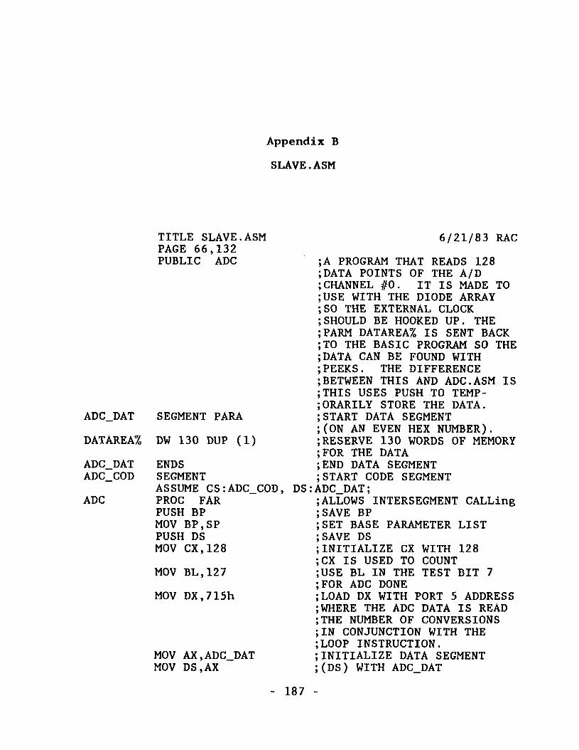
Appendix B

SLAVE.ASM

ADC_DAT

DATAREA%ADC_DATADC_COD

ADC

TITLE SLAVE.ASM PAGE 66,132 PUBLIC ADC

SEGMENT PARA

DW 130 DUP (1)ENDSSEGMENTASSUME C S :ADC_C0D,PROC FARPUSH BPMOV B P ,SPPUSH DSMOV C X ,128MOV BL,127MOV DX,715h

MOV A X ,ADC_DAT MOV D S ,AX

6/21/83 RAC;A PROGRAM THAT READS 128 ;DATA POINTS OF THE A/D ;CHANNEL #0. IT IS MADE TO ;USE WITH THE DIODE ARRAY ;SO THE EXTERNAL CLOCK ;SHOULD BE HOOKED UP. THE ;PARM DATAREA% IS SENT BACK ;TO THE BASIC PROGRAM SO THE ;DATA CAN BE FOUND WITH ;PEEKS. THE DIFFERENCE ;BETWEEN THIS AND ADC.ASM IS ;THIS USES PUSH TO TEMP­O R A R I L Y STORE THE DATA.;START DATA SEGMENT ;(ON AN EVEN HEX NUMBER).;RESERVE 130 WORDS OF MEMORY ;FOR THE DATA ;END DATA SEGMENT ;START CODE SEGMENT

D S :ADC_DAT;;ALLOWS INTERSEGMENT CALLing ;SAVE BP;SET BASE PARAMETER LIST ;SAVE DS;INITIALIZE CX WITH 128 ;CX IS USED TO COUNT ;USE BL IN THE TEST BIT 7 ;FOR ADC DONE;LOAD DX WITH PORT 5 ADDRESS ;WHERE THE ADC DATA IS READ ;THE NUMBER OF CONVERSIONS ;IN CONJUNCTION WITH THE ;LOOP INSTRUCTION.;INITIALIZE DATA SEGMENT ;(DS) WITH ADC_DAT

- 187 -

188

AGAIN: CYCLE:

RECOV:

ADCADC COD

IN A X ,DX CLI

DEC DX IN AL,DXCMP AL ,BL

JBE CYCLE

INC DX IN A X ,DXPUSH AX

LOOP AGAINSTIMOV C X ,128MOV B X ,256

POP AX MOV B X ,AX SUB B X ,2

LOOP RECOV MOV AX,DS POP DS MOV DI,BP+6MOV D I ,AXPOP BP RET 2

ENDPENDSEND

READS PORTS 5 AND 6 TO RESET DONE FLIPFLOP CLEAR INTERRUPTS BEGIN OUTER LOOP RESET DX TO PORT 4 READ PORT 4 TO CHECK FOR CONVERSION DONE. THIS IS TRUE IF THE HIGHEST BIT IS HIGH (THAT IS THE NUMBER IS 128 OR GREATER). IF NOT READ IT AGAIN.IF IT IS HIGH READ THE CONVERSION:RESET DX TO PORT 5 READS PORTS 5 AND 6 (WHICH ARE IN D X ) .TRANSFER THE DATA TO THE STACK FOR TEMP STORAGE READ A TOTAL OF {CX} POINTS END OUTER LOOP SET INTERRUPTS BACK ON INITIALIZE CX WITH 128.CX IS USED TO COUNTBX IS USED AS THE INDEX TOTHE DATA SEGMENT.REMOVE FROM STACK AND PLACE IN MEMORY INCREMENT DATA SEGMENT INDEX TO THE NEXT WORD REPEAT {CX} NUMBER OF TIMES

GET ADDRESS OF PARAMETER DATAREA%PASS BACK FIRST VALUE OF DATAREA%RESTORE BPRETURN TO BASIC WITH THE ADDRESS OF THE DATA SEGMENT (DATAREA%).END PROCEDURE END CODE SEGMENT END PROGRAM

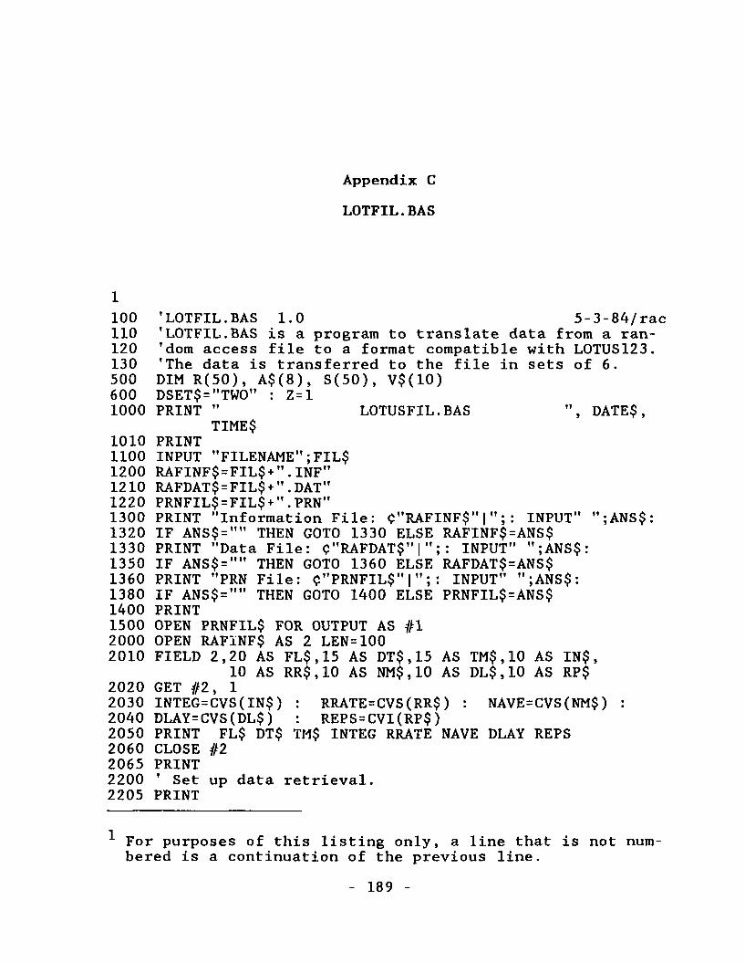
Appendix CLOTFIL.BAS

1100 'LOTFIL.BAS 1.0 5-3-84/rac110 'LOTFIL.BAS is a program to translate data from a ran-120 'dom access file to a format compatible with LOTUS123.130 'The data is transferred to the file in sets of 6.500 DIM R( 50), A $ (8), S(50), V$(10)600 DSET$="TW0" : Z=11000 PRINT " LOTUSFIL.BAS ", D ATE$,

TIME$1010 PRINT1100 INPUT "FILENAME";FIL$1200 RAFINF$=FIL$+".INF"1210 RAFDAT$=FIL$+".DAT"1220 PRNFIL$=FIL$+".PRN"1300 PRINT "Information File: <?"RAFINF$"|";: INPUT" ";ANS$: 1320 IF ANS$="” THEN GOTO 1330 ELSE RAFINF$=ANS$1330 PRINT "Data File: C"RAFDAT$"|";: INPUT" ";ANS$:1350 IF ANS$="" THEN GOTO 1360 ELSE RAFDAT$=ANS$1360 PRINT "PRN File: <?"PRNFIL$"|";: INPUT" ";ANS$:1380 IF ANS$="" THEN GOTO 1400 ELSE PRNFIL$=ANS$1400 PRINT1500 OPEN PRNFIL$ FOR OUTPUT AS #1 2000 OPEN RAF1NF$ AS 2 LEN=1002010 FIELD 2,20 AS F L $ ,15 AS D T $ ,15 AS T M $ ,10 AS I N $ ,

10 AS R R $ ,10 AS N M $ ,10 AS D L $ ,10 AS RP$2020 GET #2, 12030 INTEG=CVS(IN$) : RRATE=CVS(RR$) : NAVE=CVS(NM$) :2040 DLAY=CVS(DL$) : REPS=CVI(RP$)2050 PRINT FL$ DT$ TM$ INTEG RRATE NAVE DLAY REPS 2060 CLOSE #2 2065 PRINT2200 ' Set up data retrieval.2205 PRINT

1 For purposes of this listing only, a line that is not num­bered is a continuation of the previous line.

- 189 -

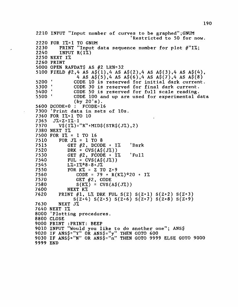
1902210 INPUT "Input number of curves to be graphed";GNUM

'Restricted to 50 for now.2220 FOR 17=1 TO GNUM2230 PRINT "Input data sequence number for plot #"I7;2240 INPUT R(l7o)2250 NEXT 1%2260 PRINT5000 OPEN RAFDAT$ AS #2 LEN=325100 FIELD #2,4 AS A$(l),4 AS A$(2),4 AS A$(3),4 AS A$(4),

4 AS A $(5),4 AS A$(6),4 AS A$(7),4 AS A$(8)5200 ' CODE 10 is reserved for initial dark current.5300 ' CODE 30 is reserved for final dark current.5400 ' CODE 50 is reserved for full scale reading.5500 ' CODE 100 and up are used for experimental data

(by 2 0 ’s ).5600 DCODE=0 : FC0DE=167300 'Print data in sets of 10s.7360 FOR 17=1 TO 10 7365 J7=Z+I7-17370 V$(I7)="R"+MID$(STR$(J7),2)7380 NEXT 177500 FOR 17 = 1 TO 167510 FOR J7o = 1 TO 87515 GET #2, DC0DE + 1% ’Dark7520 DRK = CVS(A$(J%))7530 GET #2, FCODE + 1% ’Full7540 FUL = CVS(A$(J7))7545 L7=l7*8-8+J77550 FOR K% = Z TO Z + 97560 CODE = 79 + R(K7)*20 + 1%7570 GET #2, CODE7580 S(K7o) = CVS(A$( J%) )7600 NEXT K%7620 PRINT #1, L7o DRK FUL S(Z) S(Z+1) S(Z + 2) S(Z + 3)

S(Z + 4) S(Z + 5 ) S(Z + 6 ) S(Z + 7 ) S(Z + 8) S(Z + 9)7630 NEXT J%7640 NEXT 1%8000 'Plotting procedures.8800 CLOSE9000 PRINT :PRINT: BEEP9010 INPUT "Would you like to do another one"; ANS$9020 IF ANS$="Y" OR ANS$="y" THEN GOTO 6009030 IF ANS$="N" OR ANS$="n" THEN GOTO 9999 ELSE GOTO 90009999 END

Appendix DSASFIL.BAS

1100 ’SASFIL.BAS 1.4 1-7-84/rac (9-20-83)110 'SASFIL.BAS is a program to translate data from a ran- 120 'dom access file to a format compatible with SAS. The 140 'data is transferred to the SAS file in sets of 10.150 'This accommodates the restriction of 80 column width 140 'imposed by SAS.500 DIM R(50), A $ (8), S(50), V$(10)600 DSET$="TWO" : Z=11000 PRINT " SASFILE.BAS ", DATE$,

TIME$1010 PRINT1100 INPUT "FILENAME";FIL$1200 RAFINF$=FIL$+".INF"1210 RAFDAT$=FIL$+".DAT"1220 SASFIL$=FIL$+".SAS"1300 PRINT "Information File: <?"RAFINF$"|";: INPUT" ";ANS$: 1320 IF ANS$="" THEN GOTO 1330 ELSE RAFINF$=ANS$1330 PRINT "Data File: C"RAFDAT$"|";: INPUT" ";ANS$:1350 IF ANS$="" THEN GOTO 1360 ELSE RAFDAT$=ANS$1360 PRINT "SAS File: C"SASFIL$"|";: INPUT" ";ANS$:1380 IF ANS$="" THEN GOTO 1390 ELSE SASFIL$=ANS$1390 INPUT "Would you like the dark and full scale plotted";

DPLT$:1400 PRINT1500 OPEN SASFIL$ FOR OUTPUT AS #1 2000 OPEN RAFINF$ AS 2 LEN=1302010 FIELD 2,20 AS F L $ ,15 AS D T $ ,15 AS T M $ ,10 AS I N$,10 AS

R R $ ,10 AS N M $ ,10 AS D L $ ,10 AS R P $ ,10 AS EM$,20 AS S$ 2020 GET #2, 12030 INTEG=CVS(IN$) : RRATE=CVS(RR$) : NAVE=CVS(NM$) :2040 DLAY=CVS(DL$) : REPS=CVI(RP$)2050 PRINT FL$ DT$ TM$ INTEG RRATE NAVE DLAY REPS EM$

For purposes of this listing only, a line that is not num­bered is a continuation of the previous program line.

- 191 -

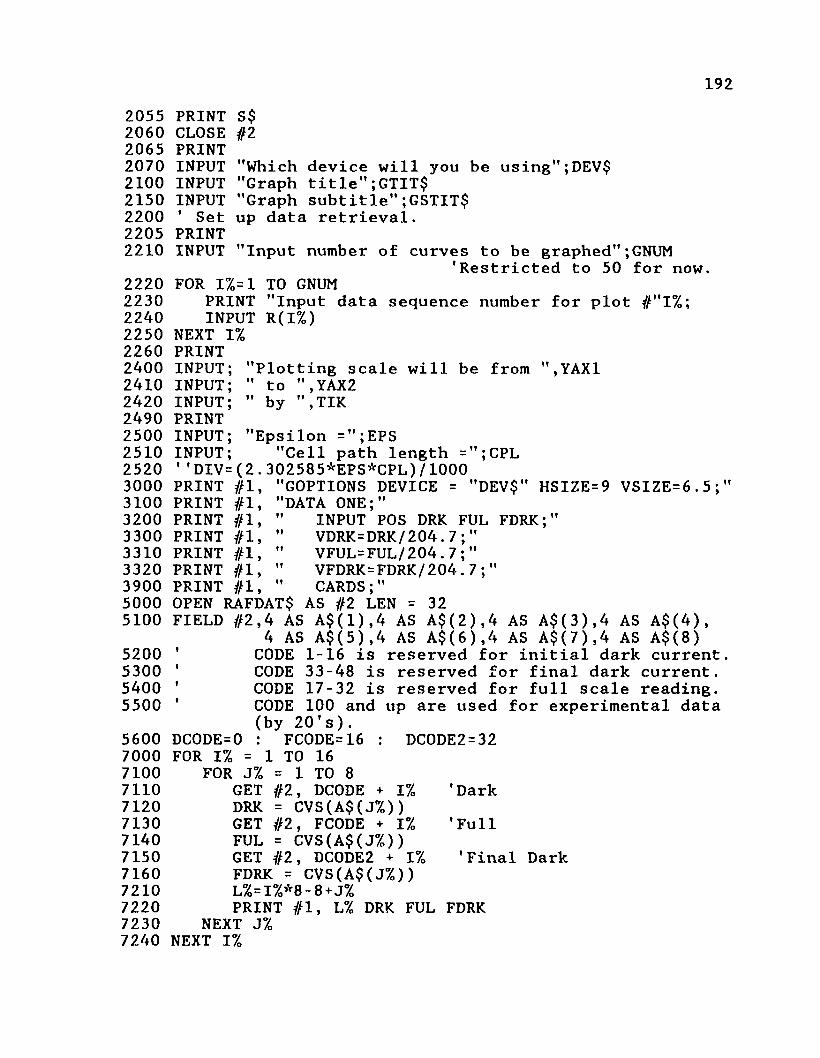
192205520602065207021002150220022052210222022302240225022602400241024202490250025102520300031003200330033103320390050005100

5200530054005500

5600700071007110712071307140715071607210722072307240

PRINT CLOSE PRINT INPUT INPUT INPUT ' Set PRINT INPUT

S$#2"Which device will you be using";DEV$ "Graph title";GTIT$"Graph subtitle";GSTIT$ up data retrieval.

"Input number of curves to be graphed";GNUM'Restricted to 50 for now.

FOR I%=1 TO GNUMPRINT "Input data sequence number for plot #"I%; INPUT R(I%)

NEXT I%PRINT

Plotting scale will be from ",YAX1 to ",YAX2 by ",TIK

INPUT;INPUT;INPUT;PRINT INPUT;INPUT;''DIV=(2.302585*EPS*CPL)/1000

Epsilon =";EPS"Cell path length =";CPL

PRINTPRINTPRINTPRINTPRINTPRINTPRINT

#1,#1 ,#1 ,#1,#1 ,#1,#1,

= "DEV$" HSIZE=9 VSIZE=6.5;" FDRK;"

GOPTIONS DEVICE DATA ONE;"

INPUT POS DRK FUL VDRK=DRK/204.7;"VFUL=FUL/204.7;"VFDRK=FDRK/204.7;"CARDS;"

OPEN RAFDAT$ AS #2 LEN = 3 2FIELD #2,4 AS A $ ( 1),4 AS A$(2),4 AS A$(3),4 AS A$(4),

4 AS A $ ( 5 ) ,4 AS A$(6),4 AS A$(7),4 AS A$(8)' CODE 1-16 is reserved for initial dark current' CODE 33-48 is reserved for final dark current.' CODE 17-32 is reserved for full scale reading.' CODE 100 and up are used for experimental data

(by 20's ).DCODE=0 : FC0DE=16 : DCODE2=32FOR 1% = 1 TO 16

FOR J% = 1 TO 8GET #2, DCODE + 1%DRK = CVS(A$(J % ) )GET #2, FCODE + 1%FUL = CVS(A$(J % ) )GET #2, DCODE2 + 1%FDRK = CVS(A$(J%))L%=l7o*8-8 + J%PRINT #1, L% DRK FUL FDRK

NEXT J%NEXT 1%

'Dark'Full

Final Dark

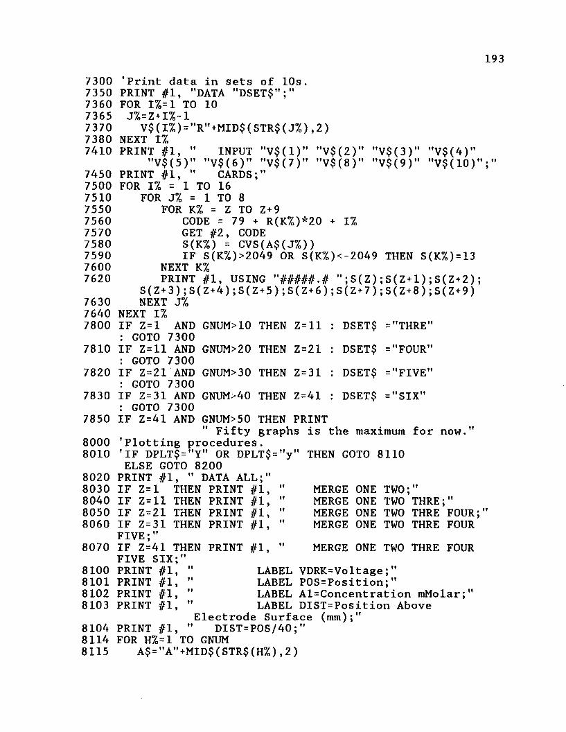
1937300735073607365737073807410

7450750075107550756075707580759076007620763076407800

7810

782078307850

80008010

8020803080408050806080708100810181028103810481148115

’Print data in sets of 10s.PRINT #1, ’’DATA "DSET$";"FOR I%=1 TO 10 J%=Z+I%-1

V $ (1 % )="R”+MID$(STR$(J % ),2)NEXT 17oPRINT #1, " INPUT ”V$(1)” "V$(2)” "V$(3)M "V$(4)"

"V$(5)" ”V$(6)” "V$(7)" "V$(8)" "V$(9)” "V$(10)";" PRINT #1, " CARDS;"FOR 1% = 1 TO 16

FOR J% = 1 TO 8FOR K Z = Z TO Z+9

CODE = 79 + R(K%)*20 + 1%GET #2, CODE S(K%) = CVS(A$(J % ) )IF S(K%)>2049 OR S(K%)<-2049 THEN S(K%)=13

NEXT K%PRINT #1, USING "#####.# ";S(Z);S(Z+l);S(Z+2);

S (Z + 3 ) ;S(Z+4);S(Z+5); S (Z + 6); S (Z + 7); S (Z + 8); S (Z + 9) NEXT J%

NEXT 1%IF Z=1 AND GNUM>10 THEN Z=ll : GOTO 7300IF Z=ll AND GNUM>20 THEN Z=21 : GOTO 7300IF Z=21 AND GNUM>30 THEN Z=31 : GOTO 7300IF Z=31 AND GNUM>40 THEN Z=41 : GOTO 7300IF Z=41 AND GNUM>50 THEN PRINT

" Fifty graphs is the maximum for now." 'Plotting procedures.'IF DPLT$="Y" OR DPLT$="y" THEN GOTO 8110 ELSE GOTO 8200

PRINT #1, " DATA ALL;"IF Z=1 THEN PRINT #1,IF Z=ll THEN PRINT #1,IF Z=21 THEN PRINT #1,IF Z=31 THEN PRINT #1,FIVE;"IF Z=41 THEN PRINT #1,FIVE SIX;"PRINT #1, " LABEL VDRK=Voltage;PRINT #1, " LABEL POS=Position;PRINT #1, " LABEL Al=Concentration mMolar;"PRINT #1, " LABEL DIST=Position Above

Electrode Surface (mm);"PRINT #1, " DIST=POS/40;"FOR H %=1 TO GNUM

A$="A"+MID$(STR$(H%),2)

DSET$ ="THRE"

DSET$ ="FOUR"

DSET$ ="FIVE" DSET$ ="SIX"

I f

ft

I f

I f

MERGE ONE TWO;"MERGE ONE TWO THRE;" MERGE ONE TWO THRE FOUR; MERGE ONE TWO THRE FOURMERGE ONE TWO THRE FOUR

I f

f f

194811681178118 8120 813081408150816081708200821082208230830083058310832084608470848084908495850085208600880090009010902090309999

R$="R"+MID$(STR$(H%),2)PRINT #1,

NEXT H%’PRINT #1, 'PRINT #1,

"A$ ’’ = LOG ( ( FUL- DRK ) / ( "R$ " - DRK ) ) /(2.302585*’’EPS/1000"*"CPL");”

’PRINT //l, ’PRINT #1, ’PRINT #1,’PRINT #1, ’PRINT #1,

PRINT #1, ” PRINT #1, ” PRINT #1, ”

TITLE1 . C=BLACK ”GTIT$’’;” TITLE2 .C=BLACK Dark Current and Full Scale Readings SYMBOL1 1=JOIN V=NONE C=RED;” SYMB0L2 1=JOIN V=NONE C=RED;" PLOT VDRK*POS VFUL*POS/OVERLAY HAXIS=0 TO 128 BY 16

VAXIS=-10 TO 10 BY 2;PROC GPLOT;”

PROC GPLOT;"TITLE1 . C=BLACK "GTIT$" ; ’’TITLE2 . C=BLACK "GSTIT$";’’

FOR G%= 1 TO GNUMSYM$ = ’’SYMBOL" +MID$ ( STR$ ( G % ), 2)PRINT #1, " "SYM$" 1=JOIN V=NONE C=RED;"

NEXT G%PRINT #1, " PLOTFOR G%= 1 TO GNUM

A$="A"+MID$(STR$(G%),2)PRINT #1, " "A$"*DIST

NEXT G7o PRINT #1, "PRINT #1, "PRINT #1, " RUN;"CLOSEPRINT :PRINTINPUT "Would you like to do another one"; ANS$IF ANS$="Y" OR ANS$="y" THEN GOTO 600IF ANS$="N" OR ANS$="n" THEN GOTO 9999 ELSE GOTO 9000END

/OVERLAY HAXIS=0 TO 3.2 BY .8" VAXIS= "YAXl" TO "YAX2" BY "TIK";"

Appendix ECONCPRFL.BAS

1X00 f » f * » » * » * * * 1 * * ? * f » I f » f f f V V V V T f T V f I f V V f f f f f f f V V f f t t f f f 1

110 '

120 ' CONCPRFL.BAS130 ' 4/84 RAC140 ' CONCPROF.BAS is a program that creates a digital150 ' simulation of a concentration profile at an160 ' electrode surface under potential step, semi-170 ' infinite linear diffusion conditions. Input180 ' parameters are time and distance of interest.190 ' Several times at a given distance can be plotted200 ' and stored in a LOTUS compatible file or a SAS file.210 '

220 ' Two MacLaurin expansions are used to approximate230 ' the error function. The first approximation is240 ' valid for 0 <= Z <= 2 for erf(Z). This one is250 ' carried out to eleven expressions. In this case260 ' Z = x/(2(SQR(DoT))), so the first one is good for270 ' the majority of cases. For Z > 2 another expansion280 * is better. This one is carried out to seven ex-290 ' pressions.300 '310 '

1000 '

1010 'Switch to color screen.1020 '1100 DEF SEG=01110 POKE &H410, (PEEK(&H410) AND &HCF) OR &H101120 SCREEN 01130 WIDTH 40:WIDTH 801140 SCREEN 2,0,01500 '

For purposes of this listing only, a line that is not num­bered is a continuation of the previous program line.

- 195 -

1961510 'Error function approximation for 0 <= Z# <= 2.0 .1520 'This is to eleven expressions.1530 '1540 DEF FNERF1#(Z # ) = 1.128379*(Z#-((Z#-3)/3) + ((Z#-5)/10)-

((Z#-7) /42) + ((Z//--9 )/216)-(( Z#-ll) /1320) +((Z#-13)/9360)-((Z#-15)/75520!)+((Z#-17)/685440!)- ((Z#->19)/6894720!) +((Z#-21)/76204800))

1600 ’1610 'Error function approximation for Z# > 2.0 .1620 'This is to seven expressions.1630 '1640 DEF FNERF2#(Z#)=l-((2.7183-(-Z#/2))/1.7725/X#)*

(l-l/Z#+3/ (Z#-2)-15 / (Z#-3 ) + 105/ (Z#--4)- 945/(Z#-5)+10395/(Z#-6))

2000 '2010 'Get height above electrode and calculate x-axis labels 2020 '2100 LOCATE 1,12110 INPUT "Distance in mm";XDIS 'For calculation2120 XMAX=XDIS/10 'purposes the dist2130 IF XDIS=0 THEN END 'should be in cm.2140 XDIS4$=MID$(STR$(XDIS),2,4)2150 XDIS3$=MID$(STR$(XDIS*.75),2,4)2160 XDIS2$=MID$(STR$(XDIS*.50),2,4)2170 XDIS1$=MID$(STR$(XDIS*.25),2,4)2500 '2510 'Get plot type.2520 '2600 LOCATE 2,12610 INPUT "Theoretical concentration profile of

Reactant or P r o d u c t I N V $2620 IF INV$="P" OR INV$="p" THEN GOTO 28002630 IF INV$="R" OR INV$="r" THEN GOTO 2900 ELSE GOTO 26002800 '2810 'Get diffusion coefficients.2820 '2830 LOCATE 3,12840 INPUT "Product Diffusion Coefficient";PDo 2850 '2900 LOCATE 4,12910 INPUT "Reactant Diffusion Coefficient";RDo 2920 CLS3000 '3010 'Plot axis.3020 '3100 FOR X=630 TO 131 STEP -1253110 LINE (X,178)-(X,180) 'X-axis tick marks.3120 NEXT X3130 FOR Y = 180 TO 0 STEP -36

1973140 LINE (130, Y) - (132,Y) ’Y-axis tick marks.3150 NEXT Y3160 PRESET (130,0)3170 LINE-(130,180),1 'Y-axis line.3180 LINE-(630,180),1 'X-axis line.3200 'X-axis label.3210 LOCATE 25,29

:PRINT " Distance from Electrode Surface (mm)";3220 LOCATE 24,16:PRINT "0";3230 LOCATE 24,31:PRINT XDISl$;3240 LOCATE 24,47:PRINT XDIS2$;3250 LOCATE 24,63:PRINT XDIS3$;3260 LOCATE 24,76:PRINT XDIS4$;3300 'Y-axis label.3310 LOCATE 12,07: PRINT "Co/Co*"3320 LOCATE 23,13: PRINT "0.0"3330 LOCATE 19,13: PRINT "0.2"3340 LOCATE 14,13: PRINT "0.4"3350 LOCATE 10,13: PRINT "0.6"3360 LOCATE 05,13: PRINT "0.8"3370 LOCATE 01,13: PRINT "1.0"4000 '4010 'Repetitive time plotting.4020 ’4100 LOCATE 1,1 4110 INPUT "Time";T 4120 IF T=0 THEN GOTO 2000 4500 '4510 'Store data in a LOTUS compatible file.4520 '4530 LOCATE 2,14540 INPUT "Store data";D$4550 IF D$="N" OR D$="n" THEN GOTO 50004560 INPUT "File name";FLN$5000 '5010 IF INV$="R" OR INV$="r" THEN GOTO 60005020 IF INV$="P" OR INV$="p" THEN GOTO 70005030 '6000 '6010 'Reactant Concentration profile 6020 'calculation, plotting and storage.6030 '6040 X=0 'Reset X, the

distEncG Vciiricibl© •6050 IF D$="Y" OR D$="y" THEN OPEN FLN$ FOR OUTPUT AS #1 6100 FOR 1=1 TO 500 '500 points calculated.6110 X=X+XMAX/5006120 X#=X/(2*SQR(RDo*T))6200 IF X#>1.9 THEN GOTO 6300 ELSE Z#=X#6210 Y=FNERF1#(Z#)

623063006310634064006500651070007010702070307040705071007110712072007210723073007310740074107440750075108000

198GOTO 6400

Z#=2*(X#-2)Y=FNERF2#(Z#)IF Y = 1 THEN LINE -(630,0): CLOSE : GOTO 4000

IF D$="Y" OR D$="y" THEN PRINT #1, Y PSET (1+130, CINT(180-Y*180))

NEXT II

'Product Concentration profile'calculation, plotting and storage.f

X=0 'Reset X, thedistance variable.

IF D$="Y" OR D$="y" THEN OPEN FLN$ FOR OUTPUT AS #1 FOR 1=1 TO 500 '500 points calculated.

X=X+XMAX/500 X#=X/(2*SQR(PDo*T))IF X # > 1 .9 THEN GOTO 7300 ELSE Z#=X#

Y =FNERF1#(Z # )GOTO 7400

Z#=2*(X#-2)Y=FNERF2#(Z#)

Y=(SQR((RDo/PDo)))*(!-Y)IF D$="Y" OR D$="y" THEN PRINT #1, Y IF Y=0 THEN LINE -(630,180): CLOSE : GOTO 4000

PSET (1+130, CINT(180-Y*180))NEXT ICLOSE : GOTO 4000

Appendix F

CA.BAS

102030405060100110120130140150160161162170

'CA123.BAS 9-26-84/rac'A program to measure the y output of the IBM EC/225 'and to step the potential in a chronoamperometric 'experiment.'Initialization els i screen 2 0 0DIM ADC1%( 1620) \ ADC07o( 1620) , TOT! (620), VTOT!(620) ADS=&H710: 'Initializes address port for

THE LABMASTERADS1=ADS+1:ADS2=ADS+2:ADS3=ADS+3:ADS4=ADS+4:ADS5=ADS+5 :ADS6=ADS+6ADS7=ADS+7:ADS8=ADS+8:ADS9=ADS+9:ADS10=ADS+10 :ADSll=ADS+11A DS12=ADS+12:ADS13=ADS+13:A DS14=ADS+14:ADS15=ADS+15OUT ADS15,128:OUT ADS12,0 OUT ADS13,0 OUT ADS14,0 OUT ADS1,0: OUT A D S ,0:

200 CLS :LOCATE 1,1 210 PRINT "220 PRINT "230 PRINT 240 PRINT

'Activate the I/O ports'Set all bits low of port A'Set all bits LOW of port B'Set all bits low of port C'Initialize voltage output to zero (NO COMPENSATION)

CA123.BAS"9-26-84/rac"

260 PRINTD/A #1 should be connected to the auxiliary input of the IBM EC/225"and A/D channel #8 should be connected to recorder output Y."

280 PRINT 290 PRINT1000 'Routine to set voltages.1010 INPUT "Initial voltage";V0LTl

1 For purposes of this listing only, a line that is not num­bered is a continuation of the previous program line.

- 199 -

2001020 INPUT "Final voltage";VOLT2 1030 IF V0LT1<V0LT2 THF.N PLTFCT=9.9 :G0T0 1080

’Set plot scale for 1040 IF V0LT1>V0LT2 THEN PLTFCT=-9.9 ELSE GOTO 200

'oxdn or redn.1080 DECIMAL=INT(818.8*(V0LT1+.01)): ’ add to compensate

for ADC offset 1090 HIGH1=INT(DECIMAL/256): L0W1=DECIMAL-256*HIGH1 1100 IF HIGH1<0 THEN HIGH1=16+HIGHl1110 PRINT "Strike any key to begin applying potential"1120 D$=INKEY$:IF D$="" THEN 1120 1160 OUT ADS3,HIGH1: OUT ADS2,L0W11180 DECIMAL=INT(818.8*(V0LT2+.01)): ' add to compensate

for ADC offset 1190 HIGH2=INT(DECIMAL/256): LOW2=DECIMAL-256*HIGH2 1200 IF HIGH2<0 THEN HIGH2=16+HIGH2 1400 ’Routine to adjust time.1410 INPUT "Input data collection rate (pts/sec)";RAT1 1420 INPUT "Input number of data points to collect";NUM1 1430 NUM1=NUM1+10 1800 'Set experiment type.1810 INPUT "Experiment type (K3Fe(CN)6, or o-Tolidine)"

;TYPE$2000 '2010 PRINT "Strike any key to begin experiment."2020 D$=INKEY$:IF D$="" THEN 2020 3000 'Routine to collect data.3020 IF RAT1=0 THEN GOTO 14003030 CNTDWN=INT(100/RATI) ’CALC DEC COUNTDOWN NUMBER3040 IF CNTDWN<>(100/RATI) THEN PRINT "Real rate =’’CNTDWN 3050 CNTDWN$=MID$(STR$(CNTDWN),2)3060 HEXRATE=VAL("&H"+CNTDWN$): ’CONVERSION TO HEX 3070 MSB=INT(HEXRATE/256): LSB=INT(HEXRATE-256*MSB):

'DIVIDE INTO HI AND LO BYTE 3100 DONE = INP(ADS6) 'RESET DONE FLIPFLOP BY

READING HIGH BYTE 3110 OUT A D S 4 ,128 'INITIALIZE ADC3120 OUT ADS9,23 'SET DATA POINTER TO

MM REGISTER3130 OUT A D S 8 ,0:OUT ADS8,128 'BCD COUNT, ETC (see pp 23

of appendix)3140 OUT ADS9,5 'SET DATA POINTER TO

COUNTER MODE OF CLOCK 5 3210 OUT A D S 8 ,49:OUT A D S 8 ,15 'USE F 5 , OSC FREQ/10,000

(100 counts/sec.)3240 OUT ADS8,LSB:OUT ADS8,MSB 'LOAD COUNTER3250 OUT A D S 9 ,112 'START COUNTING3260 OUT A D S 4 ,132 'ENABLE START CONVERSIONS3270 OUT A D S 5 ,8 'WRITE CHANNEL NO. TO BOARD3300 FOR I%=1 TO 10

2013310 IF INP(ADS4)<128 THEN 3310:'WAIT UNTIL DONE

CONVERTING ADC0%(1%)=INP(ADS5):ADC1%(I%)=INP(ADS6)

NEXT I%OUT ADS3,HIGH2: OUT ADS2,LOW2 FOR I?o=ll TO NUM1

IF INP(ADS4)<128 THEN 3360:'WAIT UNTIL DONECONVERTING

ADC0%(I%)=INP(ADS5):ADC1%(I%)=INP(ADS6)NEXT I%OUT ADS3,HIGH1: OUT ADS2.L0W1 els'CALCULATE STORED DATA AND PRINT OUT FOR I%=1 TO NUM1

33203330334033503360337033803390339540004410443044354436 4450

4460449045004510452045304540455045604570458045904600461046204630464046504660467046804690470047104720473047404750500050105020

65536!T O T ! (I7„ ) = 2 5 6 ! *CSNG (ADC 1% (1% ) ) + CSNG ( ADC0% (1%)) IF TOT!(I%)>32767! THEN TOT!(I%)=TOT!(I%)-655 V T O T !(I%)=TOT!(1%)/(-204.7)

'LPRINT using "####.##";TOT!(0), TOT!(l), TOT!(2) T O T !(3)

PSET (I%+30,INT( (VTOT! (I7„) + 10)*10)) NEXT 1%GOSUB 8000LOCATE LOCATE LOCATE LOCATE LOCATE LOCATE LOCATE LOCATE LOCATE LINE LINE LINE LINE LINE LINE LINE LINE LINE LINE LOCATE LOCATE LOCATE LOCATE LOCATE LOCATE'plot C L S :' N= 1

8,19.1 10,1

11,1 12,113.114.116.117.1

( 34,198)- ( 34,158)- ( 34,118)- ( 34, 78)- ( 34, 38)- (627,198)- (627,158)- (627,118)- (627, 78)- (627, 38)-

25.120.215.310.35.2 2,1

"C<”u'"r""e""n""t""u""A"

PRINT PRINT PRINT PRINT PRINT PRINT PRINT PRINT PRINT

31,198) 31,158) 31,118) 31, 78) 31, 38)

630,198) 630,158) 630,118) 630, 78) 630,

PRINT PRINT PRINT PRINT PRINT

38)" - 10";"-5";"0";II c n ."10";

INPUT;ANS$ surface areaelectrode

Do=7.62E-06 : Co=l : F=9.64846E04

202510051105120

5130

5140

515051605170

FOR 1=11 TO NUM1 V=(((I-10)/10)5)IF TYPE$="K" THENY=INT(((TOT!(I )*.0048852*V)-10)*(-20)) IF TYPE$="k" THENY=INT(((TOT!(I)*.0048852*V)-10)*(-20)) IF TYPE$="0" THENY=INT(((-TOT!(I )*.0048852*V)-10)*(-20)) IF TYPE$="o" THENY=INT(((-TOT!(I)*.0048852*V)-10)*(- 20)) if y<0 or y>199 then goto 5180 PSET (1+30,Y)

5180 NEXT I6000 GOSUB B0006200 LOCATE 7,1 PRINT "E"6210 LOCATE 8,1 PRINT f t *J I f

6220 LOCATE 9,1 PRINT "e"6230 LOCATE 10,1 PRINT "c"6240 LOCATE 11,1 PRINT "t"6250 LOCATE 12,1 PRINT *»r«*6260 LOCATE 13,1 PRINT "o"6270 LOCATE 14,1 PRINT "d"6280 LOCATE 15,1 PRINT "e"6290 LOCATE 17,1 PRINT "A"6300 LOCATE 18,1 PRINT U t l

6310 LOCATE 19,1 PRINT "e"6320 LOCATE 20,1 PRINT "a"6400 LOCATE 25,3 PRINT t t i f

6410 LOCATE 20,2 PRINT i t

6420 LOCATE 15,2 PRINT i t

6430 LOCATE 10,2 PRINT h ^ t i

6440 LOCATE 5,2 PRINT i i 2 ”

6450 LOCATE 1,2 PRINT I f *2 I f

6800 LOCATE 2,1 INPUT;ANS$7000 LOCATE 3,1 INPUT" Would

70107020703070357040705070607070709072008000810081058110

this data";ANS$IF ANS$="Y" OR ANS$=My" THEN GOTO 7020 ELSE GOTO 200 'DATA STORAGE ROUTINE.

INPUT "Name of storage file";FLNM$FLNM$ = FLNM$ + ".PRN"OPEN FLNM$ FOR OUTPUT AS #1 FOR !7o=l TO 600

//l, T O T ! (1%); " , "PRINT NEXT 17o CLOSE //I

LOCATE 2,1 'SUBROUTINES ' A X I S 'LINE ( 51,197)-( 51,199) LINE (201,197)-(201,199)

INPUT;ANS$ : GOTO 200

2038120813081408150816081708200830083108320833083408350850010000

LINE LINE LINE LINE LINE LINE LINE LOCATE LOCATE LOCATE LOCATE LOCATE LOCATE RETURN STOP:

351.197501.197 51, 0

201, 0 351, 0501, 030,0)-(

2,7 2,26 2,44 2,63 2,13

24,13END

) ~ (351, ) - (501, )-( 51, ) -(201, )-(351, ) -(501, 632,199 : PRINT : PRINT : PRINT : PRINT : PRINT : PRINT

199)199)

3)3)3)3)

) * >B"0";t'g"."19";"28";"Time"Time

Appendix G MEMTRAN.BAS

1

1415 DIM EDRK(128) 'Experimental darkcurrent reading.

1845 L WAT=.23125 LOCATE 10,5

:PRINT "Delay between individual laser pulses =";3265 LOCATE 10,50 :PRINT " "LWAT3691 LWAT$ = CHR$(PEEK(1538)) + CHR$(PEEK(1540) ) +

CHR$(PEEK(1542))+ CHR$(PEEK(1544))3692 LWAT$=LWAT$ +CHR$(PEEK(1546)) : LWAT=VAL(LWAT$)3700 REPS$=CHR$(PEEK(1698))+CHR$(PEEK(1700))+

CHR$(PEEK(1702)) + CHR$(PEEK(1704))3710 REPS$=REPS$ +CHR$(PEEK(1706)) : REPS=VAL(REPS$)3778 LCNT=3000*LWAT4590 OUT ADSl,HIGH14595 OUT ADS,LOWl6040 MULT=3.0:INTGl=INTG*MULT 'MULT=scan rate/33333,

which is 100000 here.

8110 OUT A D S 8 ,08115 OUT A D S 8 ,128: ’BCD count, etc. (see pp 23 of app.)8140 OUT A D S 8 ,498145 OUT A D S 8 ,15 'Set clock 3 up for no gating,

count rising8220 OUT ADS8,LSB

For purposes of this listing only, a line that is not num­bered is a continuation of the previous program line.

- 204 -

2058225 OUT ADS8,MSB 'Load counter of clock 3 load

register.8240 OUT ADS9,68 'Load counter 3. (pp 9)8260 'Set up clock 5 for laser pulsing.8270 OUT ADS9,23: 'Set data pointer to MM register.8280 OUT A D S 8 ,08285 OUT A D S 8 ,128: 'BCD count, etc. (see pp 23 of app.)8290 OUT ADS9,5 'Set data pointer to counter mode

of clock 4.8300 OUT A D S 8 ,178305 OUT ADS8,11 'Set clock 5 up for no gating,

count once,8310 'bed count, count down, osc.

freq., etc. (pp 24 Fig 7)8320 LSB=INT(2):MSB=INT(0)8330 OUT ADS8,LSB8335 OUT ADS8,MSB 'Load clock 5 load register with 2

(minimum).8340 OUT ADS9,80 'Load counter 5. (pp 9)8350 'Set up clock 4 for reading the diode array.8360 OUT ADS9,23: 'Set data pointer to MM register.8370 OUT A D S 8 ,08375 OUT A D S 8 ,128: 'BCD count, etc. (see pp 23 of app.)8380 OUT ADS9,4 'Set data pointer to counter mode of

clock 4.8390 OUT A D S 8 ,178395 OUT ADS8,11 'Set clock 4 like clock 5.8400 CNTDWN=1000*DLAY-0 'Calculate decimal

countdown.8410 CNTDWN$=MID$(STR$(CNTDWN),2)8420 HEXRATE=VAL("&H"+CNTDWN$) 'Convert to hex.8430 MSB=INT(HEXRATE/256) 'Divide into Most

Significant Byte and 8440 LSB=INT(HEXRATE-256*MSB) 'Least Significant Byte.8450 OUT ADS8,LSB8455 OUT ADS8,MSB 'Load counter of clock 4 load register. 8460 OUT ADS9,72 'Load counter 4. (pp 9)8470 PRINT "Clocks are set."8480 RETURN12245 for q=l to LCNT : next q12250 DEF SEG=DATAREA7o 'DATAREA7 is where the

data is stored.12260 FOR JZ=2 TO 256 STEP 212270 EXPMI%(H7o, 1%, J% / 2) = ( 256*PEEK( J7o+1) + PEEK( J7o) )12280 NEXT J7o12290 NEXT 1%12300 NEXT H%12310 G0SUB 22000 'Data reduction and storage.12400 'Store, plot, and print FINAL full scale data.

20612410 C L S : LOCATE 2,2: PRINT ’’Full Scale ’’ :

' LOCATE 3,2: PRINT T M $ ;12420 GOSUB 18120 ’Raw data plot.12430 LOCATE 22,1: INPUT ’’Is this OK";ANS$12435 IF ANS$="Y" OR ANS$ = ”y ” GOTO 1250012440 IF ANS$="N” OR ANS$="n" THEN GOTO 12450

ELSE GOTO 1241012450 INPUT "Recollect full scale data"; ANS$12460 IF ANS$="Y" OR ANS$="y" THEN GOTO 1200012470 IF ANS$="N" OR ANS$="n" THEN GOTO 12310

ELSE GOTO 1245012500 FOR I% = 1 TO 12812510 SAM(l7o) = IDRK(I%) - SAM(l7o)12520 NEXT 1%12530 CLS:LOCATE 2,2: PRINT "Dark Corr. " :

’ LOCATE 3,2: PRINT T M $ ;12540 GOSUB 1930012550 LOCATE 22,1: INPUT "Is this OK";ANS$12560 IF ANS$="Y" OR ANS$="y" GOTO 1260012570 IF ANS$="N" OR ANS$="n" THEN GOTO 12450

ELSE GOTO 12550 12600 LOCATE 22,1: PRINT SPACE?(15);12610 IF PRT$ = "Y" OR PRT$="y" THEN GOSUB 18000

: LPRINT CHR?(12)12620 IF DFPRT$="Y" OR DFPRT$="y" THEN GOSUB 1616012630 IF DSK$ ="Y" OR DSK$ ="y" THEN CODE=17: GOSUB 1680012640 INPUT "Should the data be normalized?";NORM$12650 INPUT "Should the experiment be run unattended?";

ATT$12700 IF EXM$="L" OR EXM$="1" THEN GOTO 12710 ELSE RETURN12710 LPRINT12720 LPRINT IDRK(20)-SAM(20),IDRK(40)-SAM(40),

IDRK(60)-SAM(60),IDRK(80) - SA M ( 8 0 ),IDRK(100)-SAM(100)12730 LPRINT12800 RETURN

14000 ’’’Experimental14100 'Set up clock14101 OUT ADS9, 22014102 OUT A D S 9 ,23:14103 OUT A D S 8 ,014104 OUT A D S 8 ,128:14105 OUT A D S 9 ,31410614107 OUT A D S 8 ,4914108 OUT A D S 8 ,15

14109 if rrat>60 then

data collection.3 for experimental data collection.

'Disable clocks 3,4 & 5 (app. pp 10) 'Set data pointer to MM register.'BCD count, etc. (see pp 23 of app, 'Set data pointer to counter mode of clock 3.'(pp 14, fig. 3 and pp 23, fig 4).

'Set clock 3 up for no gating, count rising

rr=rrat-60 else rr=rrat

)

14110

1412014130141401415014151141551416014165141701421014220142301424014250142601430014301143051431014320144001441014420

14430

1444014450145001451014520145301454014600146051461014620146301464014650146601467014680

207CNTDWN=100*RR-0 'Calculate decimal

countdown number.CNTDWN$=MID$(STR$(CNTDWN),2)HEXRATE=VAL("&H"+CNTDWN$) 'Conversion to hex.MSB=INT(HEXRATE/256) 'Divide into most

significant byte and LSB=INT(HEXRATE-256*MSB) 'least significant byteif rrat>60 then msb=msb+96print "msb="msb OUT ADS8,LSB OUT ADS8,MSB

lsb=" lsb

OUT ADS9,68 LOCATE 12,1: PRINT LOCATE 13,1: PRINT LOCATE 14,1: INPUT CLS : D=INP(ADS6)OUT ADS9, 36input "clock 3 should be FOR I% = OREPS TO REPS ' a$=inkey$IF I%=1 THEN GOTO 14320 CALL A D C (DATAREA7)PRINT I%FOR J% = I TO NAVE7+1

OUT ADS9,40 CALL A D C (DATAREA%)

'Load counter clock 3 load 'Load counter

"Return to "begin data"; "collection",ANS$

ofregister.3. (pp 9)

'Enable (arm) clock 3 (pp 9) running",ans$

OUT ADS9,56

CALL A D C (DATAREA7) for q=l to LCNT : DEF SEG=DATAREA%

'Pulses scan sequencer only. 'ADC IS A CALL IN THE ASSEMBLER SUBRT SLAVE. 'Pulse laser, DLAY, then pulse scan sequencer. 'READ LASER PULSED ARRAY,

next q'DATAREA7 is where the data is stored.

FOR K7=2 TO 256 STEP 2EXPMI%( 17a, J% ,K%/2 ) = (256*PEEK(K%+1) +PEEK(K%) )

NEXT K%NEXT J%'Collect dark current.FOR J%=1 TO 128 : EDRK(J%)=0 : NEXT J%FOR J7o = 1 TO NAVE7o

'Pulse scan sequencer ONLY. 'Read array. ADC is an assembler call in SLAVE. 'DATAREA7 is where the data is stored.

FOR K%=2 TO 256 STEP 2 EDRK(K % )2)=EDRK(K % /2) + (2 5 6 *PEEK(K%+1) + PEEK(K % ))

NEXT K7o NEXT J%

OUT ADS9,40 CALL A D C (DATAREA7)

DEF SEG = DATAREA7o

14690147001471014920

149301494014950150001501015020150301510015110151201513015140151501516015170152001521015220152301524015250152601527015300153101531315314153151531615317

153201533015340153501536015370

FOR J%=1 TO 128EDRK(J % )=EDRK(J%)/NAVE^

NEXT J%'Data collection timing sequence (in RRAT*2 sec

increment s)•

' DATA 6, 12, 18, 24, 30, 36, 42, 48, 54, 60, 66, 'Data collection complete.’'RETURNI f 1

'''DATA ANALYSIS AND REDUCTION:» ! tLIM=2 : A=0 L%=I%°CLS: 'IF OVLA$="N" OR OVLA$=”n ” THEN CLS LOCATE 1,1: PRINT "Uncorrected";LOCATE 2,1: PRINT " Data series";LOCATE 4,1: PRINT " (1 REPS")";LOCATE 3,1: PRINT "number: "1%FOR M7o=2 TO 10

FOR L7o=l TO 128SAM (L% ) = EXPMI%(17o,M7o,L%)EXPM(M7o,L7o) = EXPMl7o(17o,M7o,L7o)

NEXT L%IF PLT$="R" OR PLT$="r" THEN GOSUB 18120 IF PLT$="C" OR PLT$="c" THEN GOSUB 18700 IF PLT$="A" OR PLT$="a" THEN GOSUB 18400 IF SPRT$="Y" OR SPRT$="y" THEN GOSUB 16160

'HardcopyIF PRT$="Y" OR PRT$="y" THEN GOSUB 18000

next mCLS

' LOCATE 1,1 : INPUT "Should the data benormalized?";NORM$

IF NORM$="A" OR NORM$="a" THEN GOTO 15317 IF NORM$="Y" OR NORM$="y" THEN GOTO 15320 IF NORM$="N" OR NORM$="n" THEN GOTO 15470

ELSE GOTO 15313FOR M7=2 TO 10

FOR L%=1 TO 128SAM(L%) = EXPMl7o(17o,M7o,L7o)

NEXT L7oD=L%+M%-2: C0DE=80+D*20: GOSUB 16800

NEXT M%A = 1 0 : GOTO 15550 FOR M7=2 TO 10 GOSUB 24000 CLS

LOCATE 1,1 LOCATE 2,1 LOCATE 4,1

'Correction factor.

PRINT " Normalized";PRINT " Data series";PRINT " (1 REPS")";

1540015410154201543015440154501546015470155001551015520155301554015550155601557015580156001561015620

156501566015670156801600016800168051681016820168301684016850168601687016900169101692016930169601840018410184301844018445

209LOCATE 3,1: PRINT "number: "1%IF PLT$="R" OR PLT$="r" THEN GOSUB 18120IF PLT$="C" OR PLT$="c" THEN GOSUB 18700IF PLT$="A" OR PLT$="a" THEN GOSUB 18400IF SPRT$="Y" OR SPRT$="y" THEN GOSUB 16160

'Hardcopy.IF PRT$="Y" OR PRT$="y" THEN GOSUB 18000

NEXT M7oGOSUB 24100 'Statistical Analysis.

'Dark correction.FOR M% = 1 TO 128

SAM(M/£) = EDRK(M/£) - SAM(M7)NEXT M%CLS:LOCATE 2,2: PRINT "Dark Corr. "

:' LOCATE 3,2: PRINT T M $ ;GOSUB 19300' LOCATE 22,1: INPUT "Is this OK";ANS$GOTO 15600' IF ANS$="N" OR ANS$="n" THEN GOTO 12450

ELSE GOTO 15560'Data Storage.D=I%+AIF DSK$="Y" OR DSK$="y" THEN CODE=80+D*20

: GOSUB 16800NEXT 1%DONE$="Y" 'Return to initial potential." OUT ADSl,HIGH1: OUT ADS,L0W1 RETURN

'Data storage subroutine.FOR Q%= 1 TO 128 STEP 8

LSET A$=MKS$(SAM(Q%))LSET B$=MKS$(SAM(Q%+1))LSET C$=MKS$(SAM(Q%+2))LSET D$=MKS$(SAM(Q%+3))LSET E$=MKS$(SAM(Q%+4))LSET F$=MKS$(SAM(Q%+5))LSET G$=MKS$(SAM(Q%+6))LSET H$=MKS$(SAM(Q7+7))PUT #2, CODE CODE=CODE+1

NEXT Q%RETURN'Absorbance plot.

IF 0VLA$="Y" OR 0VLA$="y" THEN GOTO 18430 ELSE CLS LOCATE 4,3: PRINT TIME$;FOR X=1 TO 128

if sam(x)=0 then goto 18480

184461845018460184701848018700187101873018735187401875018760

187701878018800192001921019230192401925019260193001932019330193401940019410194151942019430194401945019460194701947519480194901950019510195202088022105221102212022130

210if full(x)/satn(x)<0 then goto 18480 ABSN=LOG(FULL(X)/SAM(X))/2.302585 Y=ABSN*AFACT+AOFF PSET (X*4+120,Y)

NEXT X'Concentration plot.

IF 0VLA$="Y" OR 0VLA?="y" THEN GOTO 18730 ELSE CLS LOCATE 4,3: PRINT TIME$;'LOCATE 6,1:PRINT EPSLN FOR X=1 TO 128

ABSN=L0G(FULL(X)/SAM(X))/2.302585 Y=ABSN*(EPSLNB) 'A=ebc; c=A/eb;

epslnb=1000/(epsln*b) Y=Y*AFACT+AOFF 'Scale to fit graphics display,PSET (X*4+120,Y)

NEXT X'Intensity plot.IF 0VLA$="Y" OR OVLA?="y" THEN GOTO 19230 ELSE CLSLOCATE 1,1 LOCATE 2,1 LOCATE 3,1 LOCATE 5,3

PRINT SPACE?(12)PRINT "Data sequence"

"number:" R%PRINTPRINT TIME?;

FOR X=1 TO 128Y=200-INT(SAM(X)*.04884)PSET (X*4 +120,Y)

NEXT XGOSUB 19000LOCATE 9,13:PRINT "j"LOCATE 10,13:PRINT "n"LOCATE 11,13:PRINT "t"LOCATE 12,13:PRINT "e"LOCATE 13,13:PRINT "n"LOCATE 14,13:PRINT "S"LOCATE 15,13:PRINT "i"LOCATE 16,13:PRINT "t"LOCATE 17,13:PRINT "y"LOCATE 13,15:PRINT "0"LOCATE 1,13:PRINT '' + 10LOCATE 24,14:PRINT "_9LOCATE 1.1

'Plot basic data axis.

RETURNGOSUB 19230 'Plot full scale.REP=9NUM=NAVE%*REP FOR R7o= 1 TO REP

FOR S%=2 TO NAVE%+1

21122140 EXPMI%(R%,S7n,0) = 0 'Zero rejection flags22150 NEXT S%22160 NEXT R7o22170 LOCATE 1,1 : PRINT "Full Scale data reduction."22175 PRINT "NUM ="NUM22180 PRINT "Number of standard deviations for data

rejection <?"LIM"|";22190 INPUT;ANS$ : IF ANS$="" THEN GOTO 22200

ELSE LIM=VAL(ANS$)22200 FOR S%=1 TO 1222220 MEAN1(S7)=0 'Zero means22230 SD1(S%)=0 'Zero Standard deviations22240 NEXT S722300 'full means22305 NUM=NAVE%*REP22310 FOR R%=1 TO REP22320 FOR S7=2 TO NAVE7+122325 IF EXPMI%(R7,S%,0)=1 THEN NUM=NUM-122330 NEXT S%22335 NEXT R%22340 FOR R7=l TO REP22345 FOR T%=1 to 622350 FOR S%=2 TO NAVE%+122355 IF EXPMI7o(R7o,S7o,0) = 1 THEN GOTO 2236522360 MEAN 1 ( T% ) = MEAN 1 (T % ) + EXPMI7o ( R 7 , S % , 2 0*T% )22365 NEXT S%22370 NEXT T%22375 NEXT R%22380 FOR T7o=l TO 622385 MEAN1(T % )= MEAN1(T % )/NUM22390 NEXT T%22395 PRINT : PRINT "NUM="NUM : INPUT; ANS$ : CLS 22400 'full standard deviations22410 FOR R%=1 TO REP22705 FOR R%=1 TO REP : LOCATE 2+R%,3 : PRINT R7 : NEXT R%22709 FOR R%=1 TO REP23130 FOR R7o=l TO REP24110 NUM=NAVE7n : REC=024120 FOR R%= 1 TO NAVE7o+l24140 EXPM(R7,0)=0 'Zero rejection flags24160 NEXT R%24170 LOCATE 1,1 : PRINT SPACE$(12) : LOCATE 1,124175 NUM1=NUM : PRINT "NUM ="NUM

24387 IF NUM1=NUM THEN REC=REC+1

24910 IF REC=2 THEN GOTO 25000 ELSE 24170 24930 ' INPUT "Reset rejection flags";ANS$24940 ' IF ANS$="Y" OR ANS$="y" THEN GOTO 24100

21224950 ' IF ANS$="N" OR ANS$="n" THEN GOTO 24170

ELSE GOTO 2493025000 ''Series mean calculation 25010 FOR T7=l TO 12825020 SAM(T%)=025030 NEXT T%25120 FOR T%=1 TO 12825140 FOR S%=2 TO NAVE7+125150 IF EXPM(S%,0)=1 THEN GOTO 2517025160 S AM (T7o) = S AM (T7„) + EXPM (S7o, T7o)25170 NEXT S%25190 SAM(T % ) = SAM(T % )/NUM25210 NEXT T%25220 CLS : R%=I% : GOSUB 1811425225 IF ATT$="Y" OR ATT$="y" THEN RETURN25230 LOCATE 22,1 : INPUT "Is this OK";ANS$25240 IF ANS$="Y" OR ANS$="y" THEN RETURN25250 IF ANS$="N" OR ANS$="n" THEN GOTO 15110

ELSE GOTO 2523026000 '''26010 ' " CURRENT DATA STORAGE, RETRIEVAL, AND PLOTTING: 26020 '''26100 'Current data storage, using a sequential file (PRN). 26105 IF EXPM$="C" OR EXPM$="c" THEN GOTO 26110

ELSE RETURN

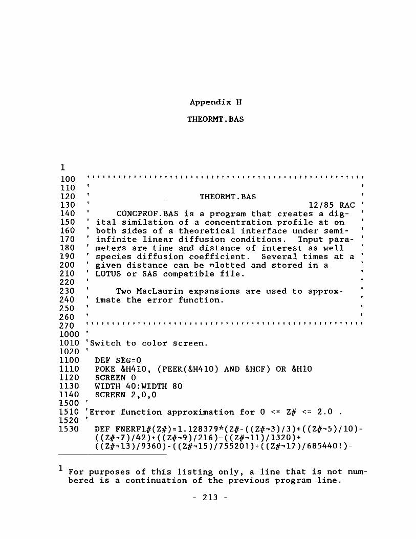
Appendix H THEORMT.BAS

1100 110 120 130 140 150 160 170 180 190 200 210 220 230 240 250 260 270 1000 1010 10201100 DEF SEG=01110 POKE &H410, (PEEK(&H410) AND &HCF) OR &H101120 SCREEN 01130 WIDTH 40:WIDTH 801140 SCREEN 2,0,01500 ’1510 'Error function approximation for 0 <= Z# <= 2.0 .1520 '1530 DEF FNERFl#(Z#)=1.128379*(Z#-((Z#-O)/3)+((Z#-5)/10)-

((Z#-7)/42)+((Z#-9)/216)-((Z#-ll)/1320)+((Z#-13 )/9360)-( (Z#-15)/75520!) + ((Z//-17 )/685440 ! )-

1 For purposes of this listing only, a line that is not num­bered is a continuation of the previous program line.

THEORMT.BAS12/85 RAC

CONCPROF.BAS is a program that creates a dig­ital similation of a concentration profile at on both sides of a theoretical interface under semi­infinite linear diffusion conditions. Input para­meters are time and distance of interest as well species diffusion coefficient. Several times at a given distance can be nlotted and stored in a LOTUS or SAS compatible file.

Two MacLaurin expansions are used to approx­imate the error function.

f f t f f V f V l f V V V f f f f V t f f V f f f f f f f T V V t f V t t f f f f f f f V f t t f f f f

Switch to color screen.

- 213 -

214((Z#-19 )/6894720! ) + ((Z#-*21) / 76204800#))

1600 '1610 ’Error function approximation for Z# > 2.0 .1620 ’1630 DEF FNERF2#(Z#)=1- ((2.7183-'(-Z#/2))/1.7725/X#)*

(1- 1/Z//+3/ (Z#-2 )-15/(Z#-3) + 105/ (Z#-4)-945/ (Z#-*5) +10395/ (Z#--6))

2000 '2010 'Get h t . above electrode and calculate x-axis labels. 2020 '2100 LOCATE 1,12110 INPUT "Distance in mm";XDIS 'For calculation2120 XMAX=XDIS/10 'purposes the2130 IF XDIS=0 THEN END 'distance should2140 XDIS4$=MID$(STR$(XDIS),2,4) 'be in cm.2150 XDIS3$=MID$(STR$(XDIS*.75),2,4)2160 XDIS2$=MID$(STR$(XDIS*.5),2,4)2170 XDIS1$=MID$(STR$(XDIS*.25),2,4)2500 ’2510 'Get plot type.2520 '2600 LOCATE 2,12610 PRINT "Theoretical concentration profile of

Membrane Transport"2620 ' IF INV$="P" OR INV$="p" THEN GOTO 2800 2630 ' IF INV$="R" OR INV$="r" THEN GOTO 2900 ELSE

GOTO 26002800 '2810 'Get diffusion coefficients.2820 '2830 LOCATE 3,12840 INPUT "Species Diffusion Coefficient";D0 2850 '2900 ' LOCATE 4,12910 ' INPUT "Reactant Diffusion Coefficient";Do 2920 CLS 3000 '3010 'Plot axis.3020 '3100 FOR X=630 TO 131 STEP -1253110 LINE (X,178)-(X,180)3120 NEXT X3130 FOR Y = 180 TO 0 STEP -363140 LINE (130,Y)-(132,Y)3150 NEXT Y3160 PRESET (130,0)3170 LINE-(130,180),13180 LINE-(630,180),13200 'X-axis label.3210 LOCATE 25,29:PRINT " Distance from Elec

'X-axis tick marks.

'Y-axis tick marks.

'Y-axis line. 'X-axis line.

215Surface (mm)";

3220 LOCATE 24,16:PRINT "0";3230 LOCATE 24,31:PRINT XDIS1$;3240 LOCATE 24,47:PRINT XDIS2$;3250 LOCATE 24,63:PRINT XDIS3$;3260 LOCATE 24,76:PRINT XDIS4$;3300 'Y-axis label.3310 LOCATE 12,7: PRINT "Co/Co*"3320 LOCATE 23,13: PRINT "0.0"3330 LOCATE 19,13: PRINT "0.2"3340 LOCATE 14,13: PRINT "0.4"3350 LOCATE 10,13: PRINT "0.6"3360 LOCATE 5,13: PRINT "0.8"3370 LOCATE 1,13: PRINT "1.0"4000 '4010 'Repetitive time plotting.4020 '4100 LOCATE 1,14110 INPUT "Time";T4120 IF T=0 THEN GOTO 20004500 '4510 'Store data in a LOTUS compatible file.4520 '4530 LOCATE 2,14540 INPUT "Store data";D$4550 IF D$="N" OR D$="n" THEN GOTO 50004560 INPUT "File name";FLN$5000 '5010 IF INV$="R" OR INV$="r" THEN GOTO 60005020 IF INV$="P" OR INV$="p" THEN GOTO 70005030 ’6000 ’6010 'Bottom Half Concentration profile 6020 'calculation, plotting and storage.6030 '6040 X=(XMAX/2)+(XMAX/128) 'Reset X, the distance.6050 IF D$="Y" OR D$="y" THEN OPEN FLN$ FOR OUTPUT AS #16100 FOR 1=1 TO 63 '64 points calc'd.6110 X=X-(XMAX/128)6120 X#=X/(2*SQR(D0*T))6200 IF X#>1.9 THEN GOTO 6300 ELSE Z#=X#6210 Y=(l-FNERFl#(Z#))/26230 GOTO 64006300 Z#=2*(X#->2)6310 Y=(l-FNERF2#(Z#))/26340 ' IF Y=1 THEN LINE -(630,0): CLOSE : GOTO 40006400 IF D$="Y" OR D$="y" THEN PRINT #1, Y6480 V=CINT((I/.256)+125)6500 PSET (V, CINT(180-Y*180))6510 NEXT I

700070107020703070407050710071107120720072107230730073107400741074407480750075108000

216

'Top Half Concentration profile 'calculation, plotting and storage.f

X=0 'Reset X, the distance variable.' IF D$="Y" OR D$="y” THEN OPEN FLN$ FOR OUTPUT AS #1

FOR 1=65 TO 128 '500 points calc'd.X=X+XMAX/128 X#=X/(2*SQR(D0*T))IF X#>1.9 THEN GOTO 7300 ELSE Z#=X#

Y=(FNERFl#(Z#)/2)+.5 GOTO 7400

Z#=2*(X#-2)Y=(FNERF2#(Z#)/2)+.5

' Y=(SQR((Do)))*(l-Y)IF D$="Y" OR D$="y" THEN PRINT #1, Y CLOSE : GOTO 4000

V=CINT((I/.256)+125)PSET (V, CINT(180-Y * 180))

NEXT ICLOSE : GOTO 4000

BIBLIOGRAPHY

1. Reid, E.W., Physiology , 26, p. 346 (1901).2. Wilson, T.H. and Wiseman, G., J. Physiology 123, p. 116

(1954).

3. Wilson, T . H . , Applied Physiolog y , 9, p. 137 (1956).

4. Crane, R.K. and T.H. Wilson, "In Vitro Method for theStudy of the Rate of Intestinal Absorption of Sugars",

Applied Physiology , 12, p. 145 (1958).

5. Shenouda, L.S. and A.M. Mattocks, "Diffusion of DrugsAcross the Isolated Mesentery", J_ Pharmaceutical Sci­ences , 56, p. 464 (1967).

6. Smith, C.M., H.F. DeLuca, Y. Tanaka, and K.R. Mahaffey,"Stimulation of Lead Absorption by Vitamin D Adminis- tratioh", Nutrition, 108, p. 843 (1978).

7. Lueck, L . M . , D.E. Wurster, T. Higuchi, A.P. Lemberger,and L.W. Busse, "Investigation and Development of Pro­tective Ointments I", American Pharmaceutical A ssoc., Scientific E d . , 46, p. 694 (1957).

8. Lueck, L . M . , D.E. Wurster, T. Higuchi, K.F. Finger,A.P. Lemberger, and L.W. Busse, "Investigation and Development of Protective Ointments II", American Pharmaceutical Assoc., Scientific Ed., 46, p. 698T1957T:

9. Lyman, D.J., B.H. Loo, and R.W. Crawford, "New Synthet­ic Membranes for Dialysis. I. A Copolyether-Ester Mem­brane System", Biochemistry, 3, p. 985 (1964).

10. Gonzales, M . A . , J. Nematollahi, W.L. Guess, and J. Autian, "Diffusion, Permeation, and Solubility of Selected Agents In and Through Polyethylene", Phar­maceutical Science s , 56, p. 1289 (1967).

- 217 -

218

11. Garrett, E.R. and P.B. Chemburkar, ’’Evaluation, Con­trol, and Prediction of Drug Diffusion Through Polymer­ic Membranes I” , J. Pharmaceutical Sciences, 57, p. 944(1968).

12. Garrett, E.R. and P.B. Chemburkar, "Evaluation, Con­trol, and Prediction of Drug Diffusion Through Polymer­ic Membranes II", J. Pharmaceutical Sciences, 57, p.949 (1968).

13. Garrett, E.R. and P.B. Chemburkar, "Evaluation, Con­trol, and Prediction of Drug Diffusion Through Polymer­ic Membranes III", J. Pharmaceutical Sciences, 57, p. 1401 (1968).

14. Patel, D.C., J.L. Fox, and W.I. Higuchi, "Physical Mod­el Approach in the Study of Alkyl Amines Across a Sili­cone Rubber Membrane in a Two Chamber Diffusion Cell", J. Pharmaceutical Sciences, 73, p. 1028 (1984).

15. Swarbrick, J., G. Lee, and J. Brom, Investigative D ermatolog y , 78, p. 63 (1982).

16. Swarbrick, J . , G. Lee, J. Brom, and P. Gensmantel,"Drug Permeation Through Human Skin II: Permeability of Ionizable Compounds", J. Pharmaceutical Sciences, 73, p. 1352 (1984).

17. Olson, C.L., T.D. Sokolowski, S.N. Pagay, and D. Michaels "Continuous Measurement of Mass Transport across Membranes", Analytical Chemistry, 41, p. 865(1969).

18. Flynn, G.L. and E.W. Smith, "Membrane Diffusion I: Design and Testing of a New Multifeatured Diffusion Cell", Jj_ Pharmaceutical Sciences, 60, p. 1713 (1971).

19. Flynn, G.L. and T.J. Roseman, "Membrane Diffusion II: Influence of Physical Adsorption on Molecular Flux through Heterogeneous Dimethylpolysiloxane Barriers",

Pharmaceutical Sciences, 60, p. 1788 (1971).

20. Flynn, G.L. and E.W. Smith, "Membrane Diffusion III: Inluence of Solvent Composition and Permeant Solubility on Membrane Transport", Pharmaceutical Sciences, 61, p. 61 (1972).

21. Chien, Y.W., Olson, C.L., and T.D. Sokoloski, "Steady State and Nonsteady-State Transport through Membranes

219

Using Rotating-Disk Electrode Polarography: Descrip­tion and Properties of a Rapid Response New Technique", J . Pharmaceutical Sciences, 62, p. 435 (1973).

22. Kuwana, T . , R.K. Darlington, and D.W. Leedy, "Electro­chemical Studies Using Conducting Glass Indicator Elec­trodes", Analytical Chemistry, 36, p. 2023 (1964).

23. Kuwana, T. and N. Winograd, "Spectroelectrochemistry at Optically Transparent Electrodes I. Electrodes Under Semi-Infinite Diffusion Conditions", in A.J. Bard, Ed., Electroanalytical Chemistry, Vol. 7, (Marcel Dekker,New York) 1974, p . 1.

24. Heineman, W .R., "Spectroelectrochemistry", AnalyticalChemistry, 50, p. 390A (March 1978).

25. Heineman, W . R . , F.M. Hawkridge, and H.N. Blount, "Spec­troelectrochemistry at Optically Transparent Elec­trodes. II. Electrodes Under Thin-Layer and Semi- Infinite Diffusion Conditions and Indirect Coulometric Titrations", in A.J. Bard, Ed., Electroanalytical Chem­istry , Vol. 13, (Marcel Dekker, New York) 1984, p. 1.

26. Tyson, J.F. and T.S. West, "Optical Absorption Phenome­na at Electrode Surfaces", Nature, 250, p. 139 (1974).

27. Tyson, J.F. and T.S. West, "Analytical Aspects ofAbsorption Spectroelectrochemistry at a Platinum Elec­trode I. Study of Metal Ions", Talanta, 26, p. 117 (1979).

28. Tyson, J.F. and T.S. West, "Analytical Aspects of Absorption Spectroelectrochemistry at a Platinum Elec­trode II. Quantitative Basis and Study of Organic Com­pounds", Talanta, 27, p. 335 (1980).

29. Pruiksma, R. and R.L. McCreery, "Observation of Elec­trochemical Concentration Profiles by Absorption Spec­troelectrochemistry", Analytical Chemistry, 51, p. 2253 (1979).

30. Pruiksma, R. and R.L. McCreery, "Spectroelectrochemical Observation of Diffusion Profiles by the Parallel Absorption Method", Analytical Chemistry, 53, p. 202 (1981).

31. Couch, R.A. and C.L. Olson, "Concentration Profile Measurement in Electrochemical Systems", 16th Annual Medicinal Chemistry M eeting, Pittsburg, 1983.

220

32. Jan, C.-C., R.L. McCreery, and F.T. Gamble, "Diffusion Layer Imaging: Spatial Resolution of Electrochemical Concentration Profiles", Analytical Chemistry, 57, p. 1763 (1985).

33. Lin, C.S., R.W. Moulton, and G.L. Putnam, "Mass Trans­fer between Solid Wall and Fluid Steams", Industrial and Engineering Chemistry, 45, p. 636 and p .640 ^1953).

34. Ibl, N . , Y. Barrada, and Trumpler, "Information on Nat­ural Convection Due to Electrolysis: Interferometric Investigation of the Diffusion Layer I.", Helvetica Chimica A c t a , 37, p. 583 (1954). (German)

35. O'Brien, R . N . , C.A. Rosenfeild, et a l ., "The Dependence of Concentration Gradient on Current Density at Wolrk- ing Electrodes", Canadian Journal of Chemistry, 43, p. 3304 (1965).

36. O'Brien, R . N . , "Concentration Gradients at Horizonal Electrodes", J. Electrochemical Society, 113, p. 389 (1966).

37. McLarnon, F.R., R.H. Muller, and C.W. Tobias, "Inter- ferometric Study of Combined Forced Convection and Nat­ural Convection", J^ Electrochemical Society: Electro­chemical Science and Technology , 129, p. 2201 (1982).

38. Kychakoff, G., Howe, R . D . , et a l ., "Visualization of Turbulent Flame Fronts with Planar Laser-Induced Fluorescence", Science , 224, p. 382 (1984).

39. Muller, S.C., T. Plesser, B. Hess, "The Structure of the Core of the Spiral Wave in the Belousov- Zhabotinskii Reaction", Science, 230, p. 661 (1985).

40. Sawyer, D . W . , J.A. Sullivan, and G.L. Mandell, "Intra- cellual Free Calcium Localization in Neutrophils During Phagocytosis", Science, 230, p. 663 (1985).

41. Steenhoek, L.E. and E.S. Yeung, "Spatial Mapping of Concentrations in Pulsed and Continuous Atom Sources", Analytical Chemistry, 53, p. 528 (1981).

42. Moore, J .H., Davis, C.C., and Coplan, M . A . , Building Scientific Apparatus, A Practical Guide to Design and Construction, (Addison-Wesley, London) 1983, chap. 4.

221

43. Webb, J.P., "Tunable Organic Dye Lasers", Analytical Chemistry, 44, 30A, (May, 1972).

44. Wright, J.C. and M.J. Wirth, "Lasers and Spectroscopy", Analytical Chemistry, 52, 988A, (Aug, 1980).

45. Wright, J.C. and M.J. Wirth, "Principles of Lasers", Analytical Chemistry , 52, 1087A, (Aug, 1980).

46. Hieftje, G .M., Travis, J.C. and Lytle, F .E., e d s ., Las­ers in Chemical Analysis, (Humana Press, Clifton, N.J.) 1981.

47. Anonymous, Molectron UV Series II Nitrogen Lasers UV 12/14 and UV 22/24, Instruction Manual (Molectron, Sun­nyvale, California) 1978, p. 1-4.

48. Meehan, E. J., "Optical Methods. Emission and Absorp­tion of Radiation", in I.M. Kolthoff and P.J. Elving, Eds. Treatise on Analytical Chemistry, 2nd E d . , Part I, vol. 7, sec. H, (Wiley, New York) 1981, chap. 1.

49. Skoog, D.A. and West, D.W. Principles of Instrumental Analysis, 2nd Ed., (Saunders, Philadelphia) 1980, chap.4.

50. Kerker, M. The Scattering of Light, (Academic Press, London) 1969, p. 19.

51. Anonymous, Molectron DL II Tunable Dye Lasers Models 12, 14, 14P Instruction Manual (Molectron, Sunnyvale, California) 1978, p. 1-6.

52. Meehan, E. J . , "Fundamentals of Spectrophotometry", in I.M. Kolthoff and P.J. Elving, Eds. Treatise on A na­lytical Chemistry, 2nd Ed., Part I, vol. 7, sec. H, (Wiley, New York) 1981, p. 68.

53. Pavia, D . L . , G.M. Lampman, and G.S. Kris, Jr., Intro­duction to Organic Laboratory Techniques, (Saunders, Philadelphia, Pa.) 1976, p. 641.

54. Meyer-Arendt, J.R., Introduction to Classical and Mod­ern Optics, 2nd Ed., (Prentice-Hall, Englewood Cliffs, N.J. ) 1984, p. 357.

55. Horlick, G., "Characteristics of Photodiode Arrays for Spectrochemical Measurements", Applied Spectroscopy,30, 113 (1976).

222

56.

57.

58.

59.

60.

61.

62.

63.

64.

65.

6 6 .

67.

68.

69.

Taltni, Y., "TV-Type Multichannel Detectors", Analytical Chemistry, 47, 699A (June, 1975).Talmi, Y . , "Applicability of TV-Type Multichannel Detectors to Spectroscopy", Analytical Chemistry, 47, 658A (June, 1975).

Sacks, R .D., "Emission Spectroscopy", in I.M. Kolthoff and P.J. Elving, Eds. Treatise on Analytical Chemis­try , 2nd Ed., Part I, vol. 7, sec. H, (Wiley, New York) 1981, chap. 6.

Horlick, G . , "Discrete Time Analog Signal Processing Devices", Analytical Chemistry, 48, 783A (Aug. 1976).Jones, D.G., "Photodiode Array Detectors in UV-Vis Spectroscopy: Part I", Analytical Chemistry, 57, 1057A(Aug. 1985).

Jones, D .G., "Photodiode Array Detectors in UV-Vis Spectroscopy: Part II", Analytical Chemistry, 57,1207A (Sept. 1985).

Anonymous, Operating Instructions for RC-1024SA Evalua­tion Board, (Reticon Corporation, Sunnyvale, Califor­nia! 1978.

Anonymous, PC-Mate LabMaster Installation Manual, (Tec- mar Inc., Cleveland, Ohio).

MacMillan, D.C. and J.H. Kroeger, Advanced Micro Devices: The Am9513 System Timing Controller^ (Advanced Micro Devices, Sunnyvale, California) 1981.Rector, R. and Alexy, G . , The 8086 B o o k , (Osborne/ McGraw Hill, Berkeley California) 1980.

Morse, S. P., The 8086/8088 Primer, 2nd Ed., (Hayden Book Co., Rochelle Park, N . j / X 1982.Anonymous, Intel iAPX 88 Book, (Reston Publishing Co., U.S.A.) 1981.Li, J. C. R . , Statistical Inference I, (Edward Broth­ers , Ann Arbor, Michigan) 1964, p. 19.

Bard, A.J., and Faulkner, L.R., Electrochemical Meth­ods, (Wiley, New York) 1980.

223

70. Galus, Z., Fundamentals of Electrochemical Analysis, (Ellis Horwood, Chichester, England) 1976, p. 97.

71. Delahay, P. New Instrumental Methods in Electrochemis­try , (Wiley Interscience, N.Y.,N.Y.) 1954, p. 415.

72. Gaylor, V . F . , P.J. Elving, and A.L. Conrad, "Polaro- graphic Oxidation of Phenolic Compounds", Analytical Chemistry, 25, p. 1078 (1953).

73. Gaylor, V.F., A.L. Conrad, and J.H. Lander1, "Use of Wax-Impregnated Graphite Electrodes in Polarography", Analytical Chemistry, 29, p. 224 (1957).

74. Flato, J.B., "The Renaissance in Polarographic and Vol- tammetric Analysis", Analytical Chemistry, 44, p. 75A (Sept. 1972).

75. Morris, J.B., and J.M. Schempf, "Voltammetric Studies at the Graphite Electrode in Quiet Solutions", Analyt­ical Chemistry, 31, p. 286 (1959).

76. Janz, G.J. and H. Taniguchi, "The Silver-Silver Halide Electrodes", Chemical Reviews, 53, p. 397 (1953).

77. Vasanavathana, S., A Study of the Application of Spec­troelectrochemistry and Metal Complex Formation of Solutions Flowing Through the Reticulated Vitreous Car­bon Electrode to Anodic Stripping Analysis, Master* s Thesis, p. 34, 1980.

78. Nicholson, R.S. and I. Shain, "Theory of Stationary Electrode Polarography", Analytical Chemistry, 36, p. 706 (1964).

79. Randles, J.E.B., Transactions Faraday Society, 44, p. 327 (1948).

80. Adams, R . N . , Electrochemistry at Solid Electrodes, (Dekker, New York) 1969.

81. Kolthoff, I.M. and J.J. Lingane, Polarography, 2nd e d . , Vol. I, (Interscience Publishers, New York) 1952, Part 1, chap. 2.

82. Laitinen, H.A. and I.M. Kolthoff, "A Study of Diffusion Processes by Electrolysis with Microelectrodes", J . American Chemical Society, 61, p. 3344, (1939).

224

83.

84.

85.

86.

87.

88.

89.

Strojek, J.W., T. Kuwana, and S.W. Feldberg, "Spectrochemical-Electrochemical Evaluation of Kinetics Using OTE", J. American Chemical Society, 90:5, p. 1353 (1968).

Strojek, J.W. and T. Kuwana, "Electrochemical Spectros­copy Using Tin Oxide-Coated OTE", Electroanalytical Chemistry, 16, p. 471 (1968).

Ostle, B. , Statistics in Research, (Iowa State College Press, Ames, Iowa) 1954~ p. 187.

Armore, S .J ., Introduction to Statistical Analysis and Inference, (Wiley, New York) 1966, p. 463.Klotz I. M . , and R. M. Rosenberg, Chemical Thermodynam­ics : Basic Theory and Methods, (W.A. Benjamin) 1972.Anonymous, Innovations in Membrane Filtration, Nucle- pore Catalog, (Nuclepore Corporation, Pleasanton, CA) 1984, p. 17.

Chien, Y.-W., Non-Steady State and Steady State Mem­brane Permeation Studied by Rotating Electrode Polarog­raphy, (Dissertation, Ohio State University, Columbus, Ohio) 1972, p. 62.