Intermediate good sourcing, wages and inequality: From ...

Rev Int Econ. 2019;27:1295–1350. wileyonlinelibrary.com/journal/roie | 1295© 2019 John Wiley & Sons Ltd

Received: 4 December 2017 | Accepted: 29 January 2019

DOI: 10.1111/roie.12400

O R I G I N A L A R T I C L E

Intermediate good sourcing, wages and inequality: From theory to evidence

Philip Luck

Economics, University of Colorado Denver, Denver, Colorado

CorrespondencePhilip Luck, University of Colorado Denver, 1380 Lawrence Street, suit 470, Denver, CO 80204.Email: [email protected]

AbstractThis paper examines the consequences of offshoring and outsourcing on domestic wages and wage inequality. I high-light the role of labor market frictions in impacting firms’ outsourcing and offshoring decisions; specifically, how dif-ferential costs of matching with workers affect the location of production (onshore or offshore) and how differential costs of assessing worker quality affect the ownership of intermediate production (intra‐firm or inter‐firm). I demon-strate how firm sourcing decisions can depend crucially on the industry skill intensity, which reflects the importance of worker–firm match quality, and as a result, the effect of offshoring on domestic labor depends on occupation and industry characteristics, as well as the ownership regime of trade. Bringing the theory to the data I rely on plausibly exogenous variation in the cost of inter‐ and intra‐firm off-shoring to identify the effects of a change in each type of offshoring on domestic wages. I find strong evidence that the effect of offshoring on domestic wages—both on the av-erage and on the wage distribution—is governed by the type of offshoring (inter‐ vs. intra‐firm), the skill intensity of the industry, and the offshorability of the occupation.

J E L C L A S S I F I C A T I O NF12; F14; F16

www.wileyonlinelibrary.com/journal/roie

mailto:

mailto:[email protected]

http://crossmark.crossref.org/dialog/?doi=10.1111%2Froie.12400&domain=pdf&date_stamp=2019-07-09

1296 | LUCK

1 | INTRODUCTION

In recent years global supply chains have become increasingly complex, crossing the borders of both countries and firms. Moreover, globalization of supply chains has led to rapid growth in the interna-tional trade of intermediate goods. From 1972 to 1990, the share of imports in the total purchase of intermediate inputs in the United States more than doubled, increasing from 5% to 11.6% (Feenstra & Hanson, 1999) and within manufacturing industries, from 2002 to 2011, this share grew by an addi-tional 30%.1 At the same time, the growth of multinational firms has also made intra‐firm trade an increasingly important component of United States trade. In 2012, intra‐firm imports made up 50.3% of the U.S.$1.13 trillion in total United States imports of goods.2 Intra‐firm imports in manufacturing accounted for half of the overall growth of total purchase of imported intermediate inputs from 2002 to 2011, outpacing the growth of inter‐firm imports. This paper investigates how the increased access to imported intermediate goods, sourced both from foreign affiliates and nonaffiliate, affects the be-havior of firms and the returns to domestic labor.

I propose a model of global production wherein the incentives for firms to source intermediates from abroad and the incentives for firms to engage in intra‐firm trade are driven by matching and screening frictions in labor markets, which generates testable predictions regarding the impacts of off-shoring on domestic wages and inequality. Specifically, I develop a framework for understanding how labor market frictions affect firm sourcing and ownership decisions, and I demonstrate theoretically and empirically how offshoring differentially affects labor depending on offshoring regime (intra‐firm or inter‐firm trade), as well as the type of industry (skill intensive or not) and the type of occupation (offshorable or not).

The model builds on the random search literature employed by Helpman, Itskhoki, and Redding (2010a, 2010b), and incorporates a model of firm intermediate good sourcing similar to Antràs and Helpman (2004, 2006). In the model, the productivity of worker–firm pairs are heterogeneous and match specific. This fact along with firm productivity heterogeneity leads to firms screening their workers with varying intensity and therefore hiring labor forces with different average skill. Additionally, since the cost of screening depends on ownership, this provides incentives for firms to take on different organizational forms. The importance of firm heterogeneity is well established in the international trade literature, and in this paper I additionally emphasize the role that labor plays in shaping observed dispersion in firm outcomes, which is supported by Irarrazabal, Moxnes, and Ulltveit‐Moe (2013) who argue that worker heterogeneity is an important source of firm observed productivity. In the theoretical model, intra‐ and inter‐firm offshoring have differential effects on productivity, which in turn allows for differential effects on domestic wages. This model also im-plies that offshoring has differential effects on wage inequality by affecting different parts of the wage distribution.3

The idea that labor market frictions may motivate trade has recently gained prominence in academic circles as well as the popular press. The New York Times recently described the role labor market frictions play in determining the location choice of multinational firms as follows: “Apple’s executives believe the vast scale of overseas factories as well as the flexibility, diligence and industrial skill of foreign workers have ... outpaced their American counterparts.”4 This quote captures the motivation for and mechanisms behind my model in two ways. First, I model the incentive to source intermediates from abroad as driven by a lower marginal cost of filling vacancies abroad, hence a more “flexible" workforce.5 In addition to shedding light on firm sourcing location decisions, the theoretical model incorporates a firm’s incentive to own their intermediate goods suppliers as being driven by the im-portance of obtaining a skilled workforce, which is easier with direct control of labor force hiring and

| 1297LUCK

screening. However, in order to realize these lower marginal costs of hiring and screening labor, firms must pay the higher fixed costs associated with international and internal production, respectively.6

Guided by the theoretical predictions of the model, this paper is the first to separately identify the differential effects of intra‐ and inter‐firm offshoring on domestic earnings. Utilizing a unique dataset that separates United States imports into related party (RP) and nonrelated party (NRP) trade flows, along with an instrumental variables strategy to identify cost‐driven changes in intra‐ and inter‐firm offshoring, I causally identify the effects of inter‐ and intra‐firm offshoring on domestic earnings. I find evidence that supports the predictions of the model: the impact of offshoring on labor markets critically depends on industry skill intensity, occupation offshorability and firm organizational form. I find that intra‐firm offshoring has a large and positive effect on earnings of those employed in nonoff-shorable occupations, while having a smaller, yet still positive, effect on earnings of those employed in offshorable occupations. This difference across occupations appears to be independent of industry skill intensity. I find that nonrelated party offshoring has a substantial negative effect on earning of those employed in nonskill intensive industries, yet this is independent of the occupation in which a worker is employed.

The estimated heterogeneous effect of intra‐ and inter‐firm offshoring are both statistically and economically significant; a one standard deviation increase in intra‐firm offshoring is predicted to increase annual earnings by as much as U.S.$15,000, while a one standard deviation increase in inter‐firm offshoring is predicted to decrease earnings by as much as U.S.$8,000.7 This is consistent with the model that predicts intra‐firm offshoring will be done by the most productive firms who, due in part to labor market frictions, pay the highest wages. I find additional evidence that the effect of intra‐firm offshoring on domestic earnings is consistent across industry groups, skill intensive vs. nonskill intensive, however it is significantly different across occupations, offshorable vs. nonoffshorable. Conversely, the effect of inter‐firm offshoring on earnings appears to be independent of occupational offshorability, while depending critically on industry characteristics.

Due in part to data limitation, previous work has traditionally either focused on the effect of total offshoring or intra‐firm offshoring on domestic labor market outcomes. The effect of total offshor-ing on domestic earnings was first investigated by Feenstra and Hanson (1999, 1996). More recently there have been many studies investigating the wage and employment effects of intermediate goods trade on domestic labor Krishna and Sethupathy (2011), Geishecker (2006), Amiti and Davis (2012), Ottaviano, Peri, and Wright (2013), and Wright (2014). Alternatively, studies such as Ebenstein, Harrison, McMillan, and Phillips (2014) and Sly, Oldenski, and Kovak (2017) have measured off-shoring using employment by foreign affiliates of multinational companies, which limits their analysis to apply only to intra‐firm offshoring.8 My results reaffirm the findings of Ebenstein et al. (2014); exposure to offshoring is dependent on occupation characteristics. Additionally, I am able to make the future contributes to the literature by developing independent measures of intra‐ and inter‐firm offshoring for a broad set of manufacturing industries, which allows me to demonstrate that exposure also depends on industry skill intensity and the type of offshoring (intra‐ vs. inter‐firm). This is the first paper to evaluate the effect of intra‐ and inter‐firm offshoring independently in a single empirical framework. Doing so I find that the empirical model does a better job fitting the data than work that disregards the role of ownership.

The remainder of the paper is organized as follows: Section 2 presents a model of production with outsourcing under labor market frictions, then Section 3 introduces offshoring which allows the model to make predictions about how offshoring affects domestic wages and wage inequality. Section 4 intro-duces the datasets employed to test the model and develops empirical tests guided by the model, and Section 5 summarizes my findings.

1298 | LUCK

2 | A MODEL OF OUTSOURCING

The model I develop utilizes firm level heterogeneity, in the form of Hicks‐neutral productivity difference, to account for the observed variation in organizational form within narrowly defined in-dustries. My model is highly stylized and produces some counter‐factual predictions, namely a strict sorting of firms based on productivity. Despite the stylized nature of the model, it provides a tractable environment that allows me to demonstrate how labor market frictions can incentivize firms’ sourc-ing and ownership decisions and how those decisions can in turn impact domestic employment and wages.

Unlike the property rights’ literature, my model relies on labor market frictions rather than incom-plete contracts to model offshoring and outsourcing. This modeling choice is supported by empirical works such as Javorcik and Spatareanu (2005) who find that flexibility in the host country’s labor mar-ket in absolute terms or relative to that in the investor’s home country, is associated with larger FDI inflows. Another important difference between this model and the literature based on Grossman and Hart (1986) is that in this model the choice to perform tasks in‐house is motivated by the gains from having direct control over the labor force, whereas the property rights literature considers vertical integration as motivated by ownership of the intermediate input itself. While control over the assets of production certainly motivates vertical integration, I argue the control over the factors of production, in this case labor, is important when considering firms operating in an environment with labor market frictions and heterogeneity in labor productivity.

In the model, individual labor productivity cannot be perfectly observed and is costlier to asses under arms‐length production, generating gains from vertical integration. Match specific workforce heterogeneity along with firm productivity heterogeneity lead to firms hiring labor forces with differ-ent average skill and provides incentives for firms to take on different organizational forms. Evidence that labor force heterogeneity plays a role in observed firm heterogeneity is provided by studies such as Irarrazabal et al. (2013) who argue that worker heterogeneity is an important source of firm ob-served productivity. Additionally, Abowd, Kramarz, and Margolis (1999) find unobserved workforce heterogeneity is an important source of wage variation, because 90% of within‐industry, across‐firm differences are explained by person fixed effects.

I will begin by describing production and consumption, once all firm decisions have been made. Then I will describe the labor markets, demonstrating how the tightness of labor markets affects the cost of production‐providing the incentive for firms to source intermediates from abroad. Next, I will detail labor force screening, which motivates some firms to produce intermediates internally. Then I will describe wage bargaining under vertical integration and outsourced production, which is unaffected by the locational choice. From there, I will solve the firm problem under all four firm alternatives (domestic outsourcing, domestic vertical integration, offshore outsourcing and offshore vertical integration). Lastly, I describe how skill intensity affects the sorting of firms by productivity and hence determine how offshoring impacts wages.9

2.1 | PreferencesAgents in this economy consume a composite good Q. I assume that utility is linear in the consump-tion of Q. Linearity results in risk neutral agents that simplify uncertainty in labor markets. When choosing which labor market to enter, workers are only concerned with the expected wage in each market.

| 1299LUCK

2.2 | ProductionProduction of the composite good Q requires two goods X and Z, combined with a Cobb–Douglas technology in a perfectly competitive market,

where I set X as the numeraire.Production in the X sector takes place under perfect competition, with no labor market frictions

and there are constant returns to the one input, labor. One unit of X is produced with one unit of labor,

This ensures that the wage in the X sector is independent of the size of the economy and is equal to PX. The inclusion of the X sector in the economy pins down the expected wage in all labor markets and gives the model the flavor of a partial equilibrium model. For this reason, the model should be viewed as an industry‐level model of the Z sector.

Production of Z requires a continuum of differentiated goods z(θ) that are combined using CES technology,

where z(θ) indicates a variety of good Z. Each z(θ) is produced by a single firm under monopolistic com-petition. Following Melitz (2003), firms can choose to enter the market by paying a fixed cost fe after which they are given a productivity draw θ from a known distribution �(�). I will assume that � is Pareto distributed:

Each firm in industry Z uses two intermediate goods—Headquarters services (H), and Production goods (G)—to produce z(θ) with the following production technology:

If a firm decides to produce, it faces a second choice regarding organizational form. Producing G in‐house requires a sizable fixed investment ( fV). Alternatively, firms can outsource the production of G, thus fac-ing a lower fixed cost of production ( fO). However, as I will detail later, this arms‐length production of G limits a firm’s ability to obtain a skilled workforce by hindering the screening process, which affects productivity and raises the marginal cost of production.

Regardless of the organizational form, labor is the sole factor of production in both intermediate goods. The labor force is ex ante identical, but upon being matched with a firm, draws match‐specific productivity from a second known distribution �(�), which is also Pareto distributed. Production of H and G is given by,

Q=Z𝜂X1−𝜂

𝜂𝜂(1−𝜂)1−𝜂, 0<𝜂<1,

X=LX .

Z =

[∫�∈Θ z(�)

�−1

� d�

] �

1−�

,

(1)�(�)=1−

(�min

�

)�

.

z(𝜃)=𝜃H𝛾G1−𝛾 , 0<𝛾 <1.

H= �̄�hn𝛽h

h, G= �̄�𝜆

gn𝛽g

g .

1300 | LUCK

I define ni as the measure of the workforce and �̄�i as the average ability of the workforce. �h and �g govern the returns to scale in production of H and G, and are assumed to be strictly positive, less than one, and satisfy 𝛽h + 𝛽g < 1. Additionally I allow for a scalar parameter λ which governs the importance of skill in production of G.10

2.3 | The labor marketThe labor market in the X sector is assumed to be perfectly competitive and without frictions. Along with the assumption of constant returns to scale, this implies that the wage in the X sector is equal to 1 (setting X as the numeraire) and pins down the outside option for workers searching for employment in sector Z. The assumption of no labor market frictions in the homogeneous goods sector is made for simplicity, and can be relaxed easily, as in Helpman and Itskhoki (2010).

The labor market in the Z sector exhibits Diamond–Mortensen–Pissarides (DMP) style random search where the number of matches in both sectors H and G are a function of the measure of vacan-cies and the measure of searching labor in each sector. Let Mi be the total matches in each industry i = h, g, the matching technology in each industry is given by a Cobb–Douglas function of vacancies created in that industry (Vi) and searching workers in that industry (Li).

Assuming that �0 is the cost of opening a vacancy, which is paid in the numeraire, the cost of a firm matching with mi workers in industry i is bimi, where bi, the cost per match, is endogenous to market con-ditions, increasing in the total number of matches and decreasing in the measure of searching labor. This leads to the following lemma.

Lemma 1 When the matching function is characterized as in Equation 2 the cost per match is endogenous to market conditions, increasing in market tightness x≡Mi∕Li, and is given by the following,

Proof Given the matching technology described in Equation 2 a firm wishing to match with m workers must post v vacancies such that v = �

−1∕�2

1x(1−�2)∕�2 m. Assuming that the cost of

opening a vacancy is given by �0, the cost per match can be expressed as � i0�

−1∕�2

1x(1−�2)∕�2,

which is equal to bi.

For simplicity I will assume identical search technology for both intermediate good sectors H and G.11 Once trade in intermediate goods is introduced, differences in the cost of filling vacancies between countries will generate an incentive for large firms, who open many vacancies, to offshore the production of G. Even though the cost of opening a vacancy �0 will be identical, differences in workers’ outside option, defined by the wage in the X sector, will generate differences in labor market tightness, which in turn will create differences in the cost of filling vacancies. In this way, factor prices drive intermediate goods trade, as in Antràs and Helpman (2004).

(2)Mi =𝜓 i1V𝜓 i

2

iL

(1−𝜓 i2)

i, 0<𝜓 i

10<𝜓 i

2<1.

(3)bi =� i0� i

1

−1∕� i2 x

1−� i2

� i2

i, xi ≡Mi∕Li.

| 1301LUCK

2.4 | Labor force screeningAfter matching with workers, the match‐specific skill of each firm’s workforce is given by G�(�), which I assume to be Pareto distributed with shape parameter k and scale parameter �min:

Once workers and firms have been matched, firms can engage in workforce screening to improve the aver-age skill of their workforce, �̄� by discarding workers with skill less than a chosen threshold �c, i. The choice of �c, i should be thought of a firms having the ability to truncate the skill distribution of its workforce. If the skill of workers is distributed Pareto, �̄� is a linear function of �c, i.

Lemma 2 When worker skill is distributed Pareto, with shape parameter k and lower support �min, for a chosen screening threshold �c, i the average skill of the workforce is given by

Proof See Appendix A.1 (for access to the Online Appendix see Supporting Information at the end of the paper).

Firms pay a cost of screening which is given by,

The cost of screening is increasing in the chosen threshold, but it is also independent of the size of the workforces. Therefore, larger firms, who employ more workers, will have an incentive to screen more heavily and achieve a more skilled workforce. As a result of search frictions and worker skill heterogene-ity, the firm’s decisions in the labor market then can be summarized by: (1) selecting a number of workers to match with for each intermediate good (mi) and (2) selecting a level of screening (�c,i) for the production of both intermediates (headquarters and production).12

When a firm chooses to outsource production of G, it outsources the matching and screening as well. In this model, sourcing intermediates from outside the firms reduces productivity, because a fraction μ < 1 of the match specific skill of the labor force in an outsourced firm is assumed to be incompatible with the match specific skill at the final good producer. Therefore, a firm which only produces the intermediate good G cannot do so as efficiently as a final good producer producing G in‐house. The intermediate good producer uses the same technology as the final good producer,

however only a fraction of the match specific skill is transferable to the final good producer such that counts toward �̄�, which alters the relationship between a firm’s chosen cutoff productivity, �c,g, and the average skill as follows:

�(�)=1−(�min

�

)k

.

�̄�i =k𝛼c,i

(k−1).

i =C𝛼c,i𝛿∕𝛿, where C>0 and 𝛿 >0.

G= �̄�𝜆gng

𝛽g ,

�̄�g = (1−𝜇)k𝛼c,g

k−1.

1302 | LUCK

The incentive for a firm to outsource production, despite the higher cost of attaining a skilled workforce, comes from the assumption that outsourced production carries with it a lower fixed cost fO < fV. Outsourcing can be thought of as accepting a higher marginal cost for a lower fixed cost, and therefore domestic outsourcing will be pursued by smaller, less productive firms.

2.5 | Post screening wage bargainingIn line with most of the random search literature, I assume that firms cannot credibly promise a wage, but that wages are determined after matching takes place through bargaining. Unlike previous work, such as Davidson, Martin, and Matusz (1999), my model will deviate from Nash bargaining and will employ a bargaining strategy put forth by Stole and Zwiebel (1996a, b) and used by Helpman et al. (2010a). Bargaining power is assumed to be equal between the firm and the workers, and that the return to being unemployed is zero.13

Under vertical integration, since bargaining takes place after all other costs including screening and matching are sunk, the wages in each intermediate good sector are given by,14

where r(nh, ng) is firm revenue and �h and �g are defined as,

and the firms share of revenue is simply the remainder, r(nh, ng)

1+�h +�g

. The firm’s organizational decision will

affect the revenue of the firm, which will in turn affect wages as can be seen in Equation 4.Under outsourced production I assume that the producer of z(θ) bargains with only the headquar-

ter’s employees, which are in their direct employ, while their partner who produces G only bargains with the production employees. Once again, assuming Stole–Zwiebel bargaining, wages of workers producing an outsourced intermediate are given by,

and wages of the headquarter’s employees at a firm that outsources G are given by

where r(nh) is the revenue of the firm producing z(θ) and outsourcing G; I will refer to this firm as the final good producing firm. Similarly, rg(ng) is the revenue of the firm producing the outsourced production good G; I will refer to this firm as the intermediate good producer.

Because of search frictions in labor markets along with skill heterogeneity in the labor force and productivity heterogeneity, firms will differ in their optimal labor force hiring and screening. Depending on their own productivity and the importance of skill, firms will choose from one of the

(4)wh =

(�h

1+�h+�g

)r(nh,ng)

nh

, wg =

(�g

1+�h+�g

)r(nh,ng)

ng

�h ≡�h��−1

�, �g ≡�g(1−�)

�−1

�,

wg =

(�g

1+�g

)rg(ng)

ng

wh =

(�h

1+�h

)r(nh)

nh

,

| 1303LUCK

following organizational structures: domestic vertically integrated production, domestic outsourced production, vertically integrated foreign production or outsourced foreign production. I will first out-line the ownership decision focusing on domestic production before introducing offshoring.

2.6 | Domestic vertical integrationThe firm choice of organizational structure will be motivated by the optimal level of matching and screening along with the relative size of fixed costs. If a firm chooses to be vertically integrated, then the production function for z(θ) is a function of matches and screening thresholds: mh, mg, �c, h, and �c, g

where �V is a combination of constants given by,

The revenue function can also be expressed as a function of matches and screening by substituting Equation 5 into the well‐known revenue function for CES aggregated goods. Therefore, the profit maxi-mizing problem of the firm is expressed by the following:

where the firms’ choice variables are matching and screening for both headquarter’s and production em-ployees: �c, h, �c, g, mh, and mg, and AZ is a demand shifter. Fixed costs are meant to embody the cost asso-ciated with building facilities for production.

Maximizing profits of the firms provides the following first‐order conditions governing the firm’s optimal employment levels

and optimal screening thresholds

Note that the optimal number of matches in the intermediate good sector H are increasing in γ, which is the cost share of H in the production of z(θ). The optimal number of matches is also decreasing in the cost of filling vacancies in each labor market, bh, and bg. Note also that if revenue is increasing in θ, the productivity of the firm, the incentive to screen a firm’s workforce is also increasing in θ.15

(5)z(�)=��Vm�g(1−�)

g m�h�

h(�c,g)(�−�gk)(1−�)(�c,h)(1−�hk)� ,

�V ≡ (�min)�hk�+�gk(1−�)(

k

k−1

)�+�(1−�)

.

ΠV (�) =max

[(1

1+�h+�g

)AZ

(��Vm

�g(1−�)

g m�h�

h�c,g

(�−�gk)(1−�)�c,h(1−�hk)�

) �−1

�

]

−(fV +C�c,g

�∕�+C�c,h�∕�+bhmh+bgmg

),

(6)(�−1)��h

�(1+�h+�g)r(�)=bhmh(�),

(�−1)(1−�)�g

�(1+�h+�g)r(�)=bgmg(�),

(7)(�−1)(1−�hk)(�)

(1+�h+�g)�r(�)=C�c,h(�)� ,

(�−1)(�−�gk)(1−�)

(1+�h+�g)�r(�)=C�c,g(�)� .

1304 | LUCK

Solving the above firm problem, I can express firm revenue as a function of the underlying param-eters given by the following:

where KV and Γ1 are combination of parameters.16 Additionally, revenue is decreasing in the cost of filling vacancies, bh, and bg, as well as in the cost of screening labor C. When a firm chooses to be vertically integrated it is able to realize the full benefit of screening. Under domestic outsourcing the cost is paid by the partner firm, but the full benefit is not realized by the final good producing firm owing to mismatch. I will now detail the firm problem under domestic outsourced production.17

2.7 | Domestic outsourcingWhen a firm outsources production of G, it outsources screening and hiring to an independent intermediate good producer. Consider a final good producer who purchases G, the production good, from a nonaffiliated firm and pays a unit price of Pg.

18 This final good producer will therefore choose �c, h, mh and G to produce z(θ). Under the assumption that both the outsourcing firm and the independ-ent intermediate producer decide on the level of production prior to bargaining over wages, the profit function of the firm can be written as:

where �o is a combination of parameters given by, �o ≡ (�min)�hk�(

k

k−1

)�

. Maximizing with respect to the

firm’s choice variables demonstrates that the intermediate good producer receives a constant share of the final good‐producing firm’s revenue, however since that revenue is decreasing in the price of the interme-diate, the intermediate good producer will maximize profits by maximizing the final good producer’s revenue, conditional on its own costs.

Intermediate good suppliers search for labor by the same method as final good producers, and therefore pay the same cost for filling vacancies (bg) and have access to the same screening technology as final good producers. Employing the first‐order conditions of the final good producer along with the derivation of wages paid to production employees, I can express the profit maximizing problem faced by the intermediate producer in terms of its own choice variables, �c, g and mg, as well as the final good producer’s revenue r(θ), which is a function of Pg:

The intermediate good producer simply receives a share of the total revenue of the final good firm minus their own costs of screening and posting vacancies. Therefore, taking headquarter’s em-ployment and average skill as given, the production good supplier chooses screening and hiring to maximize profit. The intermediate good producer chooses its level of production fully internalizing its own effect on the price of the intermediate. Even though the final good producing firm spends a

(8)rV (�)= (KV )1

Γ1

�−1

� A

1

Γ1

Z

[�b

−�h�

hb−�g(1−�)

g C−(1−�hk)�−(�−�gk)(1−�)

�

] �−1

�

1

Γ1,

ΠO(�) =max

[(1

1+�h

)AZ

(��om

�h�

h�c,h

(1−�hk)�G1−�) �−1

�

]

−(fO+C�c,h

�∕�+bhmh+G∗Pg

),

ΠG =max

{(1

1+�g

)(�−1)(1−�)

�(1+�h)r(�)−

(C�c,g

�∕�+bgmg

)}.

| 1305LUCK

constant share of revenue on the intermediate good (G), since revenue itself is decreasing in Pg, it is not optimal for the intermediate good producing firm to set this price as infinite, and the intermediate good producing firms’ problem can be summarized by the following lemma.

Lemma 3 The intermediate good producer will choose �c,g and mg such that the marginal revenue of the final good producing firm is equal to their own marginal cost of production. As such, all choice variables can be expressed in terms of the final good producers? productivity as follows,

Proof See Appendix A.2 (see Supporting Information).

Having expressed the intermediate good producer’s problem as a function of market conditions and the final good producer’s productivity, I solve for the final good producer’s revenue and profit under outsourcing, which I will show by first solving for the revenue function, and later describing the profit function:

The differences between the scaling function K under outsourcing vs. vertical integration are derived from two sources, (1) the different nature of bargaining owing to each firm only bargaining with the workers under their direct employ, and (2) the level of mismatch μ. As the mismatch grows or the importance of skill in the production good (λ) increases, the revenue of an outsourcing firm will fall.19 I highlight this fact because it provides the main incentive for firms to engage in vertical integration.

2.8 | Profits and the choices of organizational formIn order to characterize an equilibrium under autarky, I will now determine firm sorting into organiza-tional forms based on productivity. To do so, I will consider the profits under each regime, beginning with domestic vertical integration then moving to outsourcing.

Utilizing the first‐order conditions of the firm, matching and screening can be expressed as func-tions of revenue, therefore the firms share of profits can be expressed as a function of revenue and fixed costs alone:

mg(�)=(�−1

�

)2 (1−�)2�g

bg(1+�h)(1+�g)r(�)

�c,g(�)=

[(�−1

�

)2 (1−�)2(1−�gk)

C(1+�h)(1+�g)r(�)

]1∕�

(9)rO(�)= (KO)1

Γ1

�−1

�(AZ

) 1

Γ1

[�b

−�h�

hb−�g(1−�)

g C−(1−�hk)�−(�−�gk)(1−�)

�

] �−1

�

1

Γ1,

ΠV (�)=Γ1

1+�h+�g

rV (�)− fV .

1306 | LUCK

Recall that owing to bargaining, rV (�)

1+�h +�g

is the firm’s share of total revenue under vertical integration and

Γ1∕(1 + �h + �g) is the firm’s share of revenue after paying to match with and screen all employees. Lastly the firm must pay its fixed cost leaving it with ΠV (�) in profits. It will also be convenient to express profits in terms of a new function gV such that:

where gV is defined as

which along with Γ1 and σ govern the slope of the profit function with respect to productivity. Note that gV is decreasing in the cost of filling vacancies b and the cost of screening C.

By the same procedure, in the case of outsourced production, I can express matching, screening and purchases of G as a function of firm revenue, which allows me to express the profits of a firm engaging in domestic outsourcing as a function of revenue and fixed costs alone:

where Γ2 is given by,

Under outsourced production rO(�)

1+�h

is the firm’s share of total revenue and Γ2∕(1 + �h) is the share after the firm pays to match with and screen employees and purchase G. Expressing profits in terms of gO,

where gO is defined as,

For firms engaging in domestic outsourcing, the slope of the profit function with respect to productivity is governed by gO, which like gV is decreasing in the cost of filling vacancies b but unlike gV it is affected by mismatch that will lower profitability. The choice between domestic outsourcing and vertical integration therefore can be interpreted as technology choices affecting the underlying productivity of the production function, which will in turn affect employment and wages.

(10)Π(�)=gV��−1

�

1

Γ1 − fV ,

(11)gV ≡ Γ1(KV )1

Γ1

(1+�h+�g)

(AZ

) 1

Γ1

[b−�h�

hb−�g(1−�)

g C−(1−�hk)�−(�−�gk)(1−�)

�

] �−1

�

1

Γ1,

ΠO(�)=Γ2

1+�h

rO(�)− fO,

Γ2 ≡1−(�−1

�

) [�h�+ (1−�hk)∕�+ (1−�)

].

(12)ΠO(�)=gO��−1

�

1

Γ1 − fO,

(13)gO ≡ Γ2(KO)1

Γ1

(1+�h)

(AZ

) 1

Γ1

[b−�h�

hb−�g(1−�)

g C−(1−�hk)�−(�−�gk)(1−�)

�

] �−1

�

1

Γ1.

| 1307LUCK

Internalizing all aspects of the production process entails a larger fixed cost ( fO < fV), therefore in order for any firm to choose vertical integration it must be the case that gO < gV, for which the suffi-cient condition is given by,

where Λ(λ) is a combination of parameters that embodies the differences in the bargaining structures across the two organizational forms and is defined as20

Under reasonable parameter values, Λ is increasing in λ.21 The condition stated by (14), places a lower bound on the level of mismatch associated with outsourcing production of G. Given a suffi-ciently high level of mismatch (governed by μ) or a sufficiently high level of skill intensity of pro-duction of G (governed by λ) this condition can clearly be met. This condition highlights one of the crucial differences between outsourcing and vertical integration: while outsourcing allows firms to avoid high fixed costs of production as well as the cost of screening and matching, it also results in lower revenue owing to mismatch in worker skill. Most importantly, the degree to which revenue is reduced is under outsourcing governed by the magnitude of mismatch and the importance of skill in production.

One attractive feature of the model is that it allows for explicit, closed form, solutions for all firm level decision variables (matching, hiring, screening and wages). Utilizing the profit function along with the first‐order conditions of the firm under both organizational forms I can express firm specific variables in terms of these cutoff productivities, �O and �V, which represent the least productive do-mestic outsourcer and the least productive vertically integrated firm respectively.

The ability of the model to support closed form solutions for all firm choice variables allows me to show that wages are increasing in firm productivity and that the wage function is in fact discon-tinuous at the cutoff points between organizational forms. This fact is summarized in the following proposition.

Proposition 1 So long as Γ1 > 0, wages in the Z sector are increasing in firm productivity θ, and the distribution of wages is discontinuous at �V. In other words, the highest wage paid by a domes-tic outsourcer is strictly less than the lowest wage paid by a vertically integrated domestic firm.


The discontinuity of the wage function comes directly from the assumption regarding wage bar-gaining. Since wages are a function of revenue and represent the marginal profit of labor, and since the slope of the profit function is discontinuous at the cutoff productivities (�V) there is a discontinuity in the wage function at this point as well. This fact is demonstrated graphically in Figure 1, which graphs wages as a function of firm productivity and organizational form.22

(14)(1−𝜇)

𝜆(1−𝛾)𝜎−1

𝜎 <Λ(𝜆),

Λ(𝜆)≡(Γ1

Γ2

)Γ1 (1+𝜙h)

(1+𝜙h+𝜙g)

��<1

[(𝜎−1

𝜎

)1

1+𝜙g

]

��1<

−𝜎−1

𝜎(1−𝛾)[𝛽g+(𝜆−𝛽gk)∕𝛿]

,

1308 | LUCK

2.9 | Expected wages and labor market tightnessThe expected wage of a worker conditional on being matched with a firm is independent of firm pro-ductivity. This can be shown by utilizing the first‐order conditions of the firm problem along with the revenue shares determined from the bargaining problem in Equation 4 and expressing wages as a function of b, the cost of filling a vacancy and the ratio of matches to workers hired, m(�)

n(�):

F I G U R E 1 Autarky firm sorting and wages

| 1309LUCK

The above condition implies that conditional on being matched, expected wages are the same, removing the incentive to direct search. The expected wage, unconditional on matching, must also be equal across H and G in order for workers to be indifferent between searching in each intermediate good sector. The unconditional expected wage depends on the probability of being matched, which is determined by labor market tightness, x = M/L, where M is the total number of matches and L is the labor searching in the sector.

Equations 3 and 15 can be used to express both the cost of filling a vacancy and labor market tight-ness as functions of the expected wage ω:

In this model ω is determined outside the Z sector, which implies labor market tightness is the same in both intermediate good sectors as long as the same matching technology exists in both, so that bh = bg = b. Additionally, since I abstract away from labor market frictions in the X sector, the expected wage depends on the marginal productivity of labor in the X sector, which leads to the fol-lowing proposition:

Proposition 2 Both the cost of filling vacancies, b, as well as labor market tightness x are increasing in the expected wage ω, which itself is determined by the outside option of workers and is governed by the marginal productivity of labor in the X sector, which itself is constant and equal to one by virtue of setting X to the numeraire.

Proof This proposition follows directly from Equation 16 along with the assumption that the outside sector has no labor market frictions and constant returns to scale.

Proposition 2 highlights the importance of the outside option in determining the cost of production in the Z sector. A worse outside option (i.e., a lower marginal productivity of labor in the X sector) would increase the share of the labor force searching for employment in the Z sector thereby reducing labor market tightness and reducing the cost of filling vacancies. As I have shown in Equations 11 and 13 firm revenue and profits are decreasing in labor market tightness, therefore the ability to access less competitive labor markets can increase profits. This will now be introduced formally through offshore production in a country with a less productive X sector.

3 | INTRODUCTION OF OFFSHORING

At this point I will introduce a very simple model of offshoring which can be thought of as introduc-ing a new labor pool that can be used for the production of G but not for H. The foreign country has a labor pool which produces good X for consumption. Just as in the home country, X is produced with constant returns to scale technology and again labor is the only input,

(15)wi(�)=m(�)

n(�)bi, i∈{h,g}.

(16)b= �a

1

1+�b ��b

1+�b , x=

��

�a

� 1

1+�b

, where � ia≡⎛⎜⎜⎝

� i0

� i1

1∕� i2

⎞⎟⎟⎠

and � ib≡ 1−� i

2

� i2

.

1310 | LUCK

To capture the idea that workers in the foreign country have a worse outside option than domestic workers, I assume that foreign labor is less productive in the X sector. All variables associated with the foreign labor market and foreign production will be indicated with an asterisk (*).

Firms can engage in vertically integrated and outsourced offshoring by placing intermediate good production of G in the foreign country under either outsourcing or vertically integrated production. For simplicity, I assume both countries are identical in their distribution of match specific skills. As in the closed economy setting, these organizational forms carry fixed costs: f ∗

V is the fixed cost of vertical

integration in the foreign country, and f ∗O is the fixed cost of outsourcing production in the foreign

country. I assume the size of the fixed costs satisfy,

but at this point I take no stance on the cost of offshore outsourcing relative to vertically integrated domes-tic production. If a firm chooses to outsource production to an intermediary in the foreign country, they face an additional mismatch cost μ which represents the greater uncertainty in evaluating the skill level of employees at an independently owned firm. Additionally firms must incur a trade cost of t for offshored inputs.23

The incentive for firms to offshore production is derived from a lower cost of filling vacancies in the foreign country. A lower cost for filling vacancies is ensured by the lower productivity in the X sector, which pins down the expected wage in the labor market for the intermediate sector G. Using Equation 16 I can derive the cost of filling vacancies abroad as the following:

Since the foreign country has a lower expected wage 𝜔∗ < 𝜔, as a result of the poorer outside option, the cost of filling of vacancies is lower: b∗ < b.24 The lower cost of filling vacancies decreases firm costs and increases profitability.25

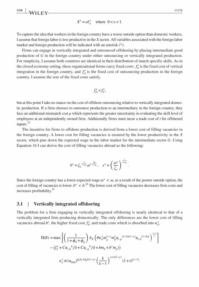
3.1 | Vertically integrated offshoringThe problem for a firm engaging in vertically integrated offshoring is nearly identical to that of a vertically integrated firm producing domestically. The only differences are the lower cost of filling vacancies abroad b∗, the higher fixed cost f ∗

V, and trade costs which is absorbed into �∗

V.

X∗ =𝜐L∗x

where 0<𝜐<1.

f ∗O< f ∗

V,

b∗ = �a

1

1+�b �∗�b

1+�b , x∗ =

(�∗

�a

) 1

1+�b

.

Π(�) =max

[(1

1+�h+�g

)AZ

(��∗

Vm1−�

gm

�

h�c,g

(�−k)(1−�)�c,h(1−k)�

) �−1

�

]

−(f ∗V+C�c,h

�∕�+C�c,g�∕�+bmh+b∗mg)

)

�∗V≡ (�min)�hk�+�gk(1−�)

(k

k−1

)�+�(1−�)

(1+ t)(�−1).

| 1311LUCK

Following the same procedure as in domestic production I can define wages and employment of vertically integrated offshorers, as well as describe profits in terms of g∗

V

where g∗V is defined as,26

It can be easily shown that gV < g∗V so long as the cost saving from offshoring production b∗ are not en-

tirely erased by trade cost t. As a result any firm who engages in vertically integrated offshoring will pay higher wages than domestic firms, leading to the following proposition.

Proposition 3 Wages for workers employed in H production are increasing in firm productiv-ity θ, and for a given level of productivity, so long as the following holds,

domestic wages are higher under vertical integrated offshoring than under domestic vertically integration.


Proposition 3 details the necessary condition under which gV < g∗V. As stated, when this condition

holds the iceberg trade cost associated with offshoring t, is more than compensated by the cost sav-ings from lower labor market frictions abroad. This feature of the model fits well with the empirical evidence that multinational firms tend to pay higher wages. It also illustrates how offshoring of pro-duction may have a positive effect on average domestic wages. The underlying mechanism governing the wage of domestic workers remains the same: under the above condition, vertically integrated offshoring caries a lower marginal cost of production, increasing the optimal level of production and employment, at higher levels of employment the returns to screening increase resulting in a higher average level of match specific skill and a more productive workforce.27

3.2 | Offshore outsourcingFirms also have the choice to engage in offshore outsourcing, in which case domestic firms match with intermediate good suppliers costlessly and write a binding contract which specifies both a quan-tity G and a price Pg, just as is possible domestically. The foreign profit maximizing intermediate good producer then has to choose the size of the workforce, ng and the level of workforce screening, �c, g in order to maximize profit, given the demand by outsourcing final goods producers. The timing of production is the same as under domestic outsourcing, therefore the final good producing firm’s problem can be written as:

(17)Π∗V

(�)=g∗V�

�−1

�

1

Γ1 − f ∗V

,

g∗V=

Γ1(K∗V

)1

Γ1

(1+�h+�g)

(AZ

) 1

Γ1

[b−�h�b∗−�g(1−�)C

−(1−�hk)�−(�−�gk)(1−�)

�

] �−1

�

1

Γ1.

(1+ t)(1−𝛾) <(

1

𝜐

)(1−𝜓2)𝛽g

,

Π(�) =max

(1

1+�h

)AZ

(��∗

om

�

h�c,h

(1−k)�G(1−�)) �−1

�

−(f ∗O+C�c,h

�∕�+bmh+G×Pg

).

1312 | LUCK

The firm’s problem can once again be solved as it was in the domestic case, where the offshoring firms revenue, profits, wages and employment are simply functions of labor market friction, general demand conditions and screening costs. I will express profits in terms of g∗

O as follows:

where I define g∗O as,28

As was the case for vertically integrated firms, it can be easily shown that gO < g∗O, so long as the cost

savings from offshoring production b∗ are not entirely erased by trade costs t. Therefore any firm who engages in offshore outsourcing will pay higher wages domestically than those engaged in domestic out-sourcing. Additionally, offshoring firms who engage in outsourcing will pay lower wages domestically than those engaging in vertically integrated offshoring. Vertical integration allows firms to have a more skilled workforce by avoiding the mismatch cost of outsourcing.

3.3 | Organizational form and productivityThe model I have constructed allows for choices of location and organizational form of production to affect firm productivity. I summarize the predictions of the model regarding firm productivity based on location and organizational form of production in Table 1. So long as mismatch is sufficiently high and domestic outsourcing is a less productive organizational form than vertical integration, therefore gO < gV and g∗

O< g∗

V. So long as the productivity of foreign labor in the outside sector (υ) and trade

costs (t) are sufficiently small then there will be gains from offshoring production under both types of organizational form, therefore gO < g∗

O and gV < g∗

V.29 Relying on no further assumptions, it is

clear that vertically integrated offshoring is the most productive type of production while domestic outsourcing is the least productive as is detailed in Table 1. The conditions governing the profitability of offshore outsourcers and vertically integrated domestic firms depends crucially on mismatch and skill intensity as well as the outside option of foreign labor. I will now discuss two possibilities and how they imply different effects of offshoring on wages.

(18)Π∗

O(�)=g∗

O�

�−1

�

1

Γ1 − f ∗O

,

g∗O=Γ2(K∗

O)

1

Γ1

(1+�h)

(AZ

) 1

Γ1

[b−�h�b∗−�g(1−�)C

−(1−�hk)�−(�−�gk)(1−�)

�

] �−1

�

1

Γ1.

T A B L E 1 Firm sorting

Offshore outsourcing (g∗O) Vertically offshoring (g∗

V)

Domestic offshoring (gO) gO < g∗O

gO < g∗O< g∗

V

Domestic vertical integration (gV) gV ≶ g∗O

gV < g∗V

Note. The above table summarizes the clear delineation of productivity given our assumptions on the cost of hiring offshore labor (resulting in gO < g∗

O and gV < g∗

V) and the cost of outsourcing (providing gO < gV and g∗

O< g∗

V). The other combinations with clear

inequalities based on these assumptions, including the productivity ranking of gO and g∗V in the top left panel, are described above.

Note, however that given these assumptions there is no clear ranking of the productivity of offshore outsourcing and domestic vertical integration (bottom right panel). This will depend critically on the relative size of the cost savings of offshoring and the cost incurred by outsourcing.

| 1313LUCK

3.4 | Skill intensity and choice of organizational formIn this model, a firm’s production decisions can be distilled to a location choice–offshore vs. onshore–and an organizational form choice–in‐house vs. outsourced production. I have argued that outsourcing will carry a lower fixed cost but at the expense of a higher marginal cost owing to mismatch. I have also argued that offshoring will carry a larger fixed cost than domestic production but will lower the marginal cost of production as a result of a lower cost of filling vacancies abroad. What remains un-clear is which has a larger effect on marginal costs: the cost of mismatch because of outsourcing or the gains from lower labor costs because of offshoring?

Along with the size of the fixed costs, the size of these contributions to marginal costs (screening and matching costs) will determine the behavior of firms and will determine how changes in the cost of offshoring will affect domestic wages. I will now consider two distinct cases. In the first case, the savings associated with offshore production outweigh the costs associated with outsourcing, which I will call a “nonskill intensive industry.” When this is true, larger more productive firms will choose offshore outsourcing rather than domestic vertical integration. In the second case, the costs associated with outsourcing outweigh the savings associated with offshore production, which I will call a “skill intensive industry.” In this case the reverse will be true and larger, more productive firms will choose domestic vertical integration rather than offshore outsourcing.

3.4.1 | Nonskill intensive industriesThe incentive to engage in vertically integrated offshoring is derived from the lower cost of filling vacancies along with the ability to avoid the mismatch of outsourced production. To see this more clearly consider the following sufficient condition for gV < g∗

O

The above condition implies that when λ is high, the cost savings from lower matching costs under off-shore production are sufficiently high relative to the additional cost of mismatch as a result of outsourcing. This condition places an upper bound on the skill intensity of production λ, a lower bound on the degree of mismatch μ, and can only be met when X sector productivity of the foreign country υ is sufficiently low. Intuitively this condition means that the costs associated with outsourcing are outweighed by the gains from offshoring, and I call this a nonskill intensive industry because this implies a limited importance of match specific skill in the production of G.30 If this condition is met, and the fixed cost of offshore out-sourcing is greater than the fixed cost of domestic vertical integration ( fV < f ∗

O) the least productive firms

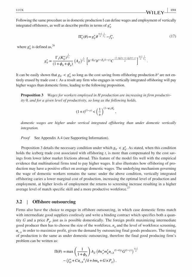
will outsource domestically, more productive firms will choose to be vertically integrated domestically, even more productive firms will be offshore outsourcers, and the most productive will engage in vertically integrated offshoring, as is illustrated in Figure 2.31

Therefore, in nonskill intensive industries, offshorers are all more productive than domestic pro-ducers, with the most productive engaging in intra‐firm trade. Additionally, since more productive firms screen more intensively and therefore pay higher wages, vertically integrated offshorers will pay the highest wages and domestic outsourcers will pay the lowest wages. Under these conditions both types of offshoring can be thought of as a more productive technology than domestic production, therefore a fall in the cost of either type of offshoring results in gains to labor, who receive a share of the profits, leaving to the following propositions.

(19)𝜐(1−𝜓2)𝛽g (1+ t)

(1−𝛾)𝜎−1

𝜎

��Offshore vacancy posting cost savings

Λ(𝜆) < (1−𝜇)𝜆(1−𝛾)

𝜎−1

𝜎

��Outsourcing mismatch cost

.

1314 | LUCK

Proposition 4 For nonskill intensive industries, a decrease in the fixed cost of vertically in-tegrated (or RP) offshoring ( f ∗

V) will increase the average wage paid to nonoffshorable occu-

pations while a fall in the cost of outsourced (or NRP) offshoring ( f ∗O) will have an ambiguous

effect on average wages.


The logic behind this proposition is relatively straightforward, vertically integrated offshorers are the largest and most productive firms utilizing the most efficient production technology—character-ized by lower cost labor market matching and screening that lower the marginal cost of production—so if the cost of this type of offshoring falls more firms will take part in vertically integrated offshoring, which will increase the wages paid out by those firms domestically, therefore increasing the average wage for those employed in the H production (nonoffshorable occupations). Conversely offshore out-sourcers are less productive, and are using a less efficient production technology, because of mismatch. Therefore, if the cost of offshore outsourcing falls it will incentivize firms to switch to offshore out-sourcing. Some of these firms, those who were vertically integrated domestic firms, will be upgrading their technology and therefore will pay higher wages, while others who were vertically integrated offshorers will be downgrading their technology and will pay lower wages. Therefore, the net effect on the average wage of those employed in H production (nonoffshorable occupations) will be ambiguous.

For those employed in G production, whose occupations can be offshored, the following proposi-tion summarizes how changes in the cost of offshoring affects average wages.

Proposition 5 For nonskill intensive industries, a decrease in the fixed cost of vertically in-tegrated (or RP) offshoring ( f ∗

V) will have no effect on the average wage paid to offshorable

occupations, while a fall in the cost of outsourced (or NRP) offshoring ( f ∗O) will decrease the

average wage paid to offshorable occupations.

F I G U R E 2 Firm profits and organizational form: Nonskill intensive industry

| 1315LUCK


A decrease in the cost of vertically integrated offshoring will only incentivize firms to switch from offshore outsourcing, and since neither of these types of firms employ worker in the production of G domestically, the average wage will be unchanged. Conversely, if the cost of offshore outsourcing falls it will incentivize firms to switch to offshore outsourcing, which will remove domestic employment in the G production. Since the jobs lost will be at the expense of the highest wage domestic employ-ment, the average wage will decrease domestically. Both of these propositions depend critically on the ordering of firms by productivity and as I have already claimed, this “nonskill intensive” sorting is only one of two possibilities.

3.4.2 | Skill intensive industriesWhen an industry is sufficiently skill intensive (λ is high) the cost savings of offshoring do not out-weigh the costs associated with outsourcing, therefore the inequality in (20) will be reversed. For these industries, vertically integrated domestic production will be more efficient than offshore out-sourcing therefore g∗

O<gV, the sufficient condition for which is

which implies that when λ is low, the cost associated with outsourcing mismatch are sufficiently high rel-ative to the gains from offshoring. Along with a different ordering of fixed costs ( f ∗

O< fV) leads offshore

outsourcers being less productive than vertical integrated domestic firms, as is illustrated in Figure 3. For skill intensive industries both types of vertical integration can be thought of as a more productive technol-ogy than outsourced production, which leads to the following propositions.

Proposition 6 For skill intensive industries a decrease in the fixed cost of vertically integrated (or RP) offshoring ( f ∗

V) will increase the average wage paid to nonoffshorable occupations while

a fall in the cost of outsourced (or NRP) offshoring ( f ∗O) will have an ambiguous effect on the

average wage.


Once again, vertically integrated offshorers are the largest and most productive firms, so a de-crease in the cost of vertically integrated offshoring will increase the average wage in the H sector as more firms take advantage of the greater productivity of vertical integration. If the cost of offshore outsourcing falls it will incentivize firms to switch to offshore outsourcing. Of these firms, the inte-grated domestic firms, will be downgrading their technology, while the domestic outsourcers will be upgrading their technology. The net effect on the average wage of those employed in H production (nonoffshorable occupations) will once again be ambiguous. These predictions are the same as in the nonskill intensive case, however for offshorable occupations wages respond differently to changes in the cost of offshoring in skill intensive industries:

(20)𝜐(1−𝜓2)𝛽g (1+ t)

(1−𝛾)𝜎−1

𝜎

��Offshore vacancy posting cost savings

Λ(𝜆) > (1−𝜇)𝜆(1−𝛾)

𝜎−1

𝜎

��Outsourcing mismatch cost

,

1316 | LUCK

Proposition 7 For skill intensive industries a decrease in the fixed cost of vertically integrated (or RP) offshoring ( f ∗

V) will decrease the average wage paid to offshorable occupations, while

a fall in the cost of outsourced (or NRP) offshoring ( f ∗O) will have an ambiguous effect on the

average wage.


In this case, a decrease in the cost of vertically integrated offshoring will incentivize switching in firms that were engaged in domestic vertical integration, thereby offshoring the highest wage G intermediate sector employment, which will drive down the average wage domestically. A decrease in the cost of offshore outsourcing will incentivize firms to switch to offshore outsourcing from both types of domestic production, this will once again have an ambiguous effect on wages, since the jobs offshored will be at both high and low wage firms.

3.5 | Offshoring wages and inequalityThe model I have developed is admittedly highly stylized, and I do not expect the predictions of Propositions 4 to 7 to hold strictly. However, the key insight of this model is that the effects of offshor-ing on domestic wages and employment depend critically on occupation and industry characteristics as well as the ownership regime of offshoring. In the following section I will test these predictions by evaluating how RP and NRP offshoring affect the average wages of those employed in offshorable and nonoffshorable occupations, for skill intensive and nonskill intensive industries.

Additionally, I will test the prediction that vertically integrated offshoring and offshore outsourcing affect average wages by influencing the industry wage distribution. My model indicates that vertically

F I G U R E 3 Firm profits and organizational form: Skill intensive industry

| 1317LUCK

integrated offshoring is performed by the most productive firms, which can be seen in Figures 2 and 3. These are also the firms who pay the highest wages, therefore a fall in the cost of vertically inte-grated offshoring should lead firms to switch from less productive organizational forms to vertically integrated offshoring. Since vertically integrated offshorers pay the highest wages this should posi-tively affect the high end of the income distribution for nonoffshorable occupations. When additional vertically integrated offshoring comes at the expense of domestic employment (as is the case for skill intensive industries) it should be by removing high wage offshorable employment.

Conversely, offshore outsourcing is done by less productive firms, therefore a fall in the cost of offshore outsourcing leads to an ambiguous effect of offshore outsourcing on average wages. This may also lead to a bunching of the wage distribution near the middle. In the following section I will develop an empirical strategy to evaluate whether vertically integrated offshoring and offshore outsourcing have differential effects on average wages as well as on the composition of the wage distribution and wage inequality.

4 | THE EFFECT OF OFFSHORING ON WAGES AND INEQUALITY

To test the key predictions of the model I will use employment and wage data along with trade flows to identify how changes in the cost of offshoring affect domestic employment and wages. The model’s predictions regarding wage inequality pertain to within industry and within occupation inequality. Therefore, in order to test these predictions I focus on within industry–occupation pair changes in wages. The identification strategy is similar throughout; I use plausibly exogenous within industry time series variation in the industry specific cost of offshoring to identify the effect of offshoring on wages of offshorable and nonoffshorable occupations. To do this, I construct an occupation specific measure of offshorability, an industry specific measure of offshoring, and an industry specific meas-ure of offshoring costs, where the latter will be used to isolate cost‐driven variation in offshoring. The construction of these measures is detailed in Section 4.1, I explore the effect of a change in the cost of offshoring on average wages within industry occupation pairs in Section 4.2 and on the wage distribution in Section 4.3.

4.1 | Description of dataIn order to measure intra‐ and inter‐firm offshoring I employ the United States Related Party Trade flows, collected by the United States Bureau of Customs and Border Protection, which distinguishes between intra‐ and inter‐firm trade. Trade flows are recorded by year, industry and source country, additionally trade is broken down by Related party (RP) or Nonrelated party (NRP) trade, where RP trade is defined as trade between two parties for which one has at least a 6% ownership share of the other. From 2002 to 2011, related party trade accounts for roughly 50% of total United States imports but varies extensively by both source country and product. For the purposes of our empirical investi-gation I will utilize RP and NRP trade as proxies for the theoretical concepts of intra‐ and inter‐firm trade in the model.

In order to evaluate the effect of offshoring on domestic wages, wage inequality, and employment I construct a measure of offshoring similar to that proposed by Feenstra and Hanson (1999) using the United States Related Party Trade flows along with industry‐level domestic production drawn from estimates in the Annual Survey of Manufactures (ASM), which allow me to construct estimates of RP and NRP offshoring separately for manufacturing industries. Using this data I generate three

1318 | LUCK

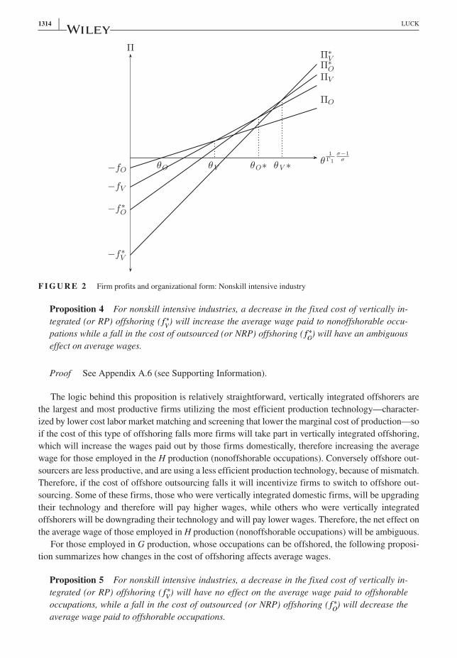
different import share measures corresponding to three different measures of offshoring: the tradi-tional “Feenstra–Hanson” measure previously described, as well as two new measures that distinguish between related party and nonrelated party offshoring, RPoff i,t and NRPoff it, constructed as follows,32

and

where �ikt is defined as intermediates purchased by industry i from industry k in time t and �it =∑

k �ikt or the sum of all intermediates purchased by industry i. IMPkt are total United States imports of k’s goods and CONSkt is domestic consumption of k, both in time t. I restrict industries k and i to have the same three‐digit NAICS code in an attempt to focus on intermediates that industry i could feasibly produce themselves.33

One concern is that observed offshoring may be influenced both by changes in the cost of off-shoring, and by domestic demand or technology shocks, which themselves may be correlated with employment and wages. To address this potential endogeneity, I use an instrumental variables ap-proach to isolate supply‐driven shocks to offshoring. I employ trade flows from China to countries other than the United States to isolate supply‐driven shocks, a method recently employed by Autor, Dorn, and Hanson (2013) and Hummels, Jorgensen, Munch, and Xiang (2014).34 Exports from China to a third‐party destination are plausibly orthogonal to United States demand and productivity shocks, but should be correlated with the Chinese productivity growth as well as changes in trade cost. The period under investigation (2002–2007) saw both remarkable increases in Chinese productivity in manufacturing as well as large decreases in trade costs as a result of China’s ascension to the WTO. Advancements in Chinese productivity most likely impact both RP and NRP offshoring similarly, however China’s WTO membership resulted in the cost of sourcing from China falling differentially according to ownership regime for two reasons: (1) China had to relax its restrictions on foreign ownership of assets in order to comply with WTO rules, which lowered the cost of RP offshoring, and (2) WTO membership normalized trade relations between China and other WTO member coun-tries, decreasing the uncertainty associated with investing in China, and also reducing the cost of RP offshoring.

I take advantage of the rich information available in the Chinese Customs Trade Statistics Data to construct two measures of Chinese exports that are meant to concord roughly to RP and NRP trade flows. RP exports from China will include Sino–foreign contractual joint ventures, Sino–foreign eq-uity joint ventures, and foreign‐owned enterprises.35 The proxy for NRP trade flows is trade that is designated as state‐owned enterprises, collective enterprises, private enterprises, or private firms. In an effort to exploit variation in the cost of trade and offshoring which is orthogonal to United States demand and technology shocks, I consider two destinations for Chinese exports. The first is Chinese exports to a set of developed economies, which are all WTO members and in aggregate sum to trade flows similar to the United States, and I will refer to this as “developed economy (DE) trade flows” for simplicity.36 In addition I also instrument the falling cost of NRP offshoring using Chinese NRP exports to the world excluding those to the United States, which will be referred to as rest of world

(21)RPoff it =

∑k

��ikt ×

�RPkt

CONSkt

��

�it

,

(22)NRPoff it =

∑k

��ikt ×

�NRPkt

CONSkt

��

�it

.

| 1319LUCK

(ROW) trade flows.37 Having constructed these three measures of trade flows, varying by industry, destination, ownership regime, and year, I then construct instruments for offshoring following a simi-lar methodology as for my measure of United States offshoring, which are the basis for my instrument set. Using United States input–output tables, I construct proxies for RP and NRP offshoring by attrib-uting Chinese exports of goods from industry k to industry i according to industry i’s use of k as an input. My developed economy instruments are given by,

while the rest of world instrument is given by,

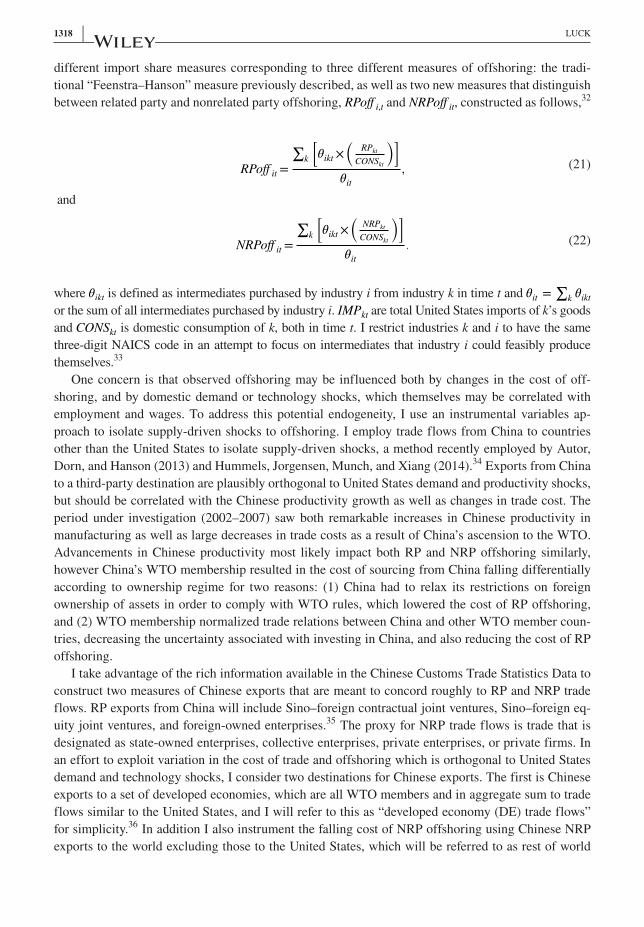
I plot the reduced form first stage of all three instruments in Figure 4. The correlation between these mea-sures is quite high resulting in a strong first stage. In our main specification, which we will introduce in the following section, our minimum first stage F‐stat is 84.9 and we strongly reject the null hypothesis of a weak first stage with both an Anderson–Rubin and Durbin–Wu–Hausman test. Additionally, throughout the sample period, United States imports from China match well with developed economy imports from China for both RP and NRP trade. Additionally, developed country RP and NRP imports from China fol-low a similar time series as United States imports for both RP and NRP flows, exhibiting a steep increase in both RP and NRP imports from China after WTO accession in 2001, which drastically reduced trade costs.

I utilize two datasets for employment and wage estimates. The first is the Occupational Employment Statistics (OES), published by the United States Bureau of Labor Statistics. The OES is constructed from a semi‐annual employer mail survey of approximately 200,000 establishments per survey and is designed to produce estimates of employment and wages for occupation–industry pairs. The OES data is well suited to address the effect of offshoring on average wages but is limited in its ability

(23)RPoff

c,de

it=

∑k �ikt ∗RP

c,de

kt

�it

, NRPoffc,de

it=

∑k �ikt ∗NRP

c,de

kt

�it

,

(24)NRPoffc,row

it=

∑k �ikt ∗NRP

c,row

kt

�it

.

F I G U R E 4 RP and NRP offshoring first stage. Note. This figure plots the reduced form first stage for both RP and NRP offshoring. As discussed in the main text, We use both instrument sets for NRP offshoring (ROW and DE) while only using DE for RP offshoring. This instrument provides a strong first stage by many metrics. The minimum F‐state across in our main specification is 84.9 and comfortably reject the null hypothesis of a weak instrument using both Anderson–Rubin and Durbin–Wu–Hausman tests [Colour figure can be viewed at wileyonlinelibrary.com]

www.wileyonlinelibrary.com

1320 | LUCK

to address the distributional effects of offshoring. Therefore, I also employ a second source, the American Community Survey (ACS) provided by Integrated Public Use Microdata Series (Ruggles, Sobek, 2010). From the ACS I use individual level employment and wage data to measure the effect of offshoring on the industry specific wage distribution.

The measure of occupation offshorability is created using occupational characteristics data from the Bureau of Labor Statistics O*NET dataset following Firpo, Lemieux, and Fortin (2011) and re-fined by Autor and Dorn (2013). Table 2 reports the five occupations with highest (least offshorable) and lowest (most offshorable) values of the index.38 This index can be thought of as a measure of how much face to face interaction an occupation requires. Unless stated, I construct a discrete variable from this index by designating 85% of occupations as offshorable, the rest nonoffshorable.39 Industry‐level skill intensity is generated by once again utilizing occupational characteristics from O*NET, related to critical thinking intensive activities, and attributing these occupation‐level measures to industries according to each occupation’s employment share in that industry. Table 3 reports the most and least skill intensive occupations by this measure. For additional details see Online Appendix I.1.2 (see Supporting Information).

In an effort to control for a vast array of alternative explanations for RP trade, I employ industry‐level data collected from multiple sources. I measure purchases of intermediates at the industry level with input–output tables published by the Bureau of Economic Analysis. Input–output tables are also used to construct measures of each industry’s position on the global value chain, following Antràs and Chor (2013). The NBER‐CES Manufacturing Industry Database provides data on industry capital, employment and value added, but annual data is only available through 2005, and since the trade data is available from 2002 through 2011 I use time invariant industry measures that are constructed by averaging annual observations from the NBER‐CES Manufacturing Industry Database over the de-cade of 1996 to 2005. Additional industry controls include industry estimates of product level demand

T A B L E 2 A measure of occupation offshorability

Occupation Index value

Lowest values

Foundry Mold and Coremakers 1.607

Pressers, Textile, Garment, and Related Materials 1.800

Mathematical Technicians 1.843

Meat, Poultry, and Fish Cutters and Trimmers 1.853

Molding, Coremaking, and Casting Machine Setters, Operators, and Tenders

1.873

Highest values

Oral and Maxillofacial Surgeons 4.543

Clinical, Counseling, and School Psychologists 4.626

Lodging Managers 4.672

Social and Community Service Managers 4.736

Clergy 4.968

Note. Following Autor and Dorn (2013) I utilize five specific activities described for each occupation, which it is argued make an oc-cupation highly nonoffshorable. These activities are: (1) establishing and maintaining personal relationships, (2) assisting and caring for others, (3) performing for or working directly with the public, (4) selling or influencing others, (5) social perceptiveness. I utilize the first four while substituting and (5) with Communicating with supervisors, peers, or subordinates. Constructing the geometric mean of these two scores Imp1∕2 ∗Lvl1∕2, then summing across attributes I construct an index of offshorability for each occupation where higher values correspond to less offshorable occupations.

| 1321LUCK

elasticities drawn from Broda and Weinstein (2006) as well as estimates of industry R&D intensity used in Nunn and Trefler (2013) and provided by the authors.40

4.2 | The effect of offshoring on average earningsThe key insight provided by the theoretical model, summarized by Propositions 4 to 7, is that the ef-fect of offshoring on domestic wages depends on occupation and industry characteristics as well as the ownership regime of offshoring. To test these predictions, I estimate the effect of RP and NRP off-shoring on earnings, allowing for differential effects based on occupation offshorability and industry skill intensity. I use occupation by industry annual earnings from the OES. Matching my measures of industry offshoring and critical thinking skill intensity along with occupation offshorability to wage and employment data from the OES provides a sample that includes 68 manufacturing industries em-ploying 503 distinct occupations. The model’s predictions regarding wage inequality pertain to within industry and within occupation inequality. Therefore, when investigating the effect of offshoring on wages, I control for industry and occupation fixed effects.

I begin by estimating the effect of total offshoring (not distinguishing RP vs. NRP) on wages, with the following model,

where OFFit is the measure of offshoring of industry i at time t, offablej is an indicator variable equal to one if occupation j is offshorable, HSi is an indicator variable equal to one if industry i’s critical thinking skill intensity is above the median, as defined in Section I.3 and �j, �i, �t are occupation, industry, and time

earningsijt = �+�1OFFit +�2OFFi,t ∗offablej+�3OFFi,t ∗HSi

+�4OFFit ∗offablej ∗HSi+�j+�i+�t + ti+�ijt,

T A B L E 3 A measure of industry skill intensity

Industry (NAICS) Index value

Lowest values

Printing and Related Support Activities (3231) 8.089

Leather Manufacturing (316M) 9.470

Tobacco Manufacturing (3122) 10.020

Apparel accessories and other apparel manufacturing (3159) 11.024

Railroad rolling stock manufacturing (3365) 11.109

Animal Slaughtering and Processing (3116) 11.377

Highest values

Agriculture, construction, and mining machinery manufacturing (3331) 14.457

Ship and Boat Building (3366) 14.843

Petroleum and Coal Products Manufacturing (3241) 14.969

Pharmaceutical and Medicine Manufacturing (3254) 15.002

Navigational, Electromedical, and Control Instruments Manufacturing (3345) 15.250

Aerospace Product and Parts Manufacturing (3364) 16.827

Note. Using my measure of occupation specific skill intensity I construct weighted averages at the industry level were weights are determined by the employment share of occupation j in industry i. For more details see Online Appendix I.3.1 (see Supporting Information).

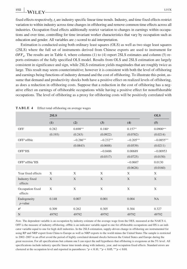
1322 | LUCK

fixed effects respectively, ti are industry specific linear time trends. Industry, and time fixed effects restrict variation to within industry across time changes in offshoring and remove common time effects across all industries. Occupation fixed effects additionally restrict variation to changes in earnings within occupa-tions and over time, controlling for time invariant worker characteristics that vary by occupation such as education and gender. All variables are z‐scored to aid interpretation.

Estimation is conducted using both ordinary least squares (OLS) as well as two stage least squares (2SLS) where the full set of instruments derived from Chinese exports are used to instrument for OFFit. The results are in Table 4, where columns (1) to (4) report 2SLS estimates and column (5) re-ports estimates of the fully specified OLS model. Results from OLS and 2SLS estimation are largely consistent in significance and sign, while 2SLS estimation yields magnitudes that are roughly twice as large. This result may seem counterintuitive; however it is consistent with both the level of offshoring and earnings being functions of industry demand and the cost of offshoring. To illustrate this point, as-sume that demand and productivity shocks both have a positive effect on realized levels of offshoring, as does a reduction in offshoring costs. Suppose that a reduction in the cost of offshoring has a neg-ative effect on earnings of offshorable occupations while having a positive effect for nonoffshorable occupations. The level of offshoring as a proxy for offshoring costs will be positively correlated with

T A B L E 4 Effect total offshoring on average wages

2SLS OLS

(1) (2) (3) (4) (5)

OFF 0.282 0.698∗∗∗ 0.180∗ 0.157∗∗ 0.0900∗∗∗

(0.193) (0.243) (0.0922) (0.0782) (0.0214)

OFF∗offble −0.286∗∗∗ −0.232∗∗∗ −0.205∗∗∗ −0.0855∗∗∗

(0.0843) (0.0688) (0.0539) (0.0211)

OFF∗HS −0.0486 0.00689 −0.00953

(0.0317) (0.0725) (0.0150)

OFF∗offble∗HS −0.0607 0.0130

(0.0626) (0.0160)

Year fixed effects X X X X X

Industry fixed effects

X X X X X

Occupation fixed effects

X X X X X

Endogeneity p‐value

0.148 0.007 0.001 0.004 NA

R2 0.309 0.262 0.305 0.304 0.327

N 49792 49792 49792 49792 49792

Note. The dependent variable is an occupation by industry estimate of the average wage from the OES, measured at the NAICS 4, OFF is the measure of industry offshoring, offble is an indicator variable equal to one for offshorable occupations and HS is an indi-cator variable equal to one for high skill industries. In the 2SLS estimation, supply‐driven change in offshoring are instrumented for using RP and NRP export from China to Europe as well as NRP exports to the world minus the United States The sample is restricted to 2002–2007 in an effort avoid the period of highly correlated demand shocks between the United States and Europe during the great recession. For all specifications but column one I can reject the null hypothesis that offshoring is exogenous at the 5% level. All specifications include industry specific linear time trends along with industry, year, and occupation fixed effects. Standard errors are clustered at the occupation level and reported in parentheses: ∗p < 0.10, ∗∗p < 0.05, ∗∗∗p < 0.01.

| 1323LUCK

the unobserved demand shocks, however, the heterogeneous effect of offshoring on earnings will cause the sign of the bias to be the opposite for offshorable and nonoffshorable occupations, leading to an attenuation for both nonoffshorable and offshorable occupations under OLS estimation.41 The fact that the OLS estimates appear to be biased in the correct direction, along with the ability to reject the null hypothesis that OFFi, t exogenous using a Durbin–Wu–Hausman test (Durbin, 1954; Wu, 1973; Hausman, 1978) in all but column (1), provides suggestive evidence that the IV strategy is necessary.

My theory makes no explicit prediction about this estimation, since estimating Equation 25 con-flates the effect of RP and NRP offshoring, however these results are broadly consistent with what other studies have found—offshoring has a positive effect on earnings for those not susceptible to offshoring, while it has a negative effect on earnings for offshorable occupations. For offshorable occupations, a one standard deviation increase in total offshoring leads to a 0.08 standard devia-tion decrease in annual earnings, approximately U.S.$1,800. Whereas for nonoffshorable occupa-tions, the same increase in total offshoring will increase annual earnings by just over U.S.$4,000.42 Additionally, I find no evidence that total offshoring differentially affects earnings depending on in-dustry skill intensity, which according to the theory developed in Section 2 is masking heterogeneity across ownership regimes.

Recall that skill intensity matters in the model because it determines the sorting of firms into RP vs. NRP offshoring, therefore I expect that not distinguishing between these two types of trade flows conceals substantial heterogeneity in the effect of offshoring. In order to test this prediction, I change the model to include both types of offshoring separately in Equation 25.

Once again offablej is an indicator variable equal to one if an occupation is offshorable, HSi is an indicator variable equal to one if an industry’s critical thinking skill intensity is above the median for all industries, �i, �j, �t are occupation, industry, and time fixed effects respectively, and ti are industry specific linear time trends. I allow for the differential effect of RP and NRP offshoring by including both measures sep-arately. This equation measures the effect of offshoring on earnings, allowing for differential effects for offshorable (offablej) occupations and skill intensive industries (HSi). Once again, I estimate (25) using 2SLS as well as OLS.

Table 5 reports my results, where the first four columns are results derived using 2SLS and column (1) reports results from the fully specified OLS model. For ease of interpretation I calculate the total effect of RP and NRP offshoring in Table 6 using coefficients from column (4), the fully specified 2SLS model.43 I find that OLS once again attenuates estimates as compared with 2SLS. This is con-sistent with the theory discussed earlier, when there are two endogenous regressors that are correlated with each other, OLS should exhibit an attenuation bias. My instruments, which should not be directly affected by United States demand or technology shocks will ameliorate this bias. For all specifications I can reject the null hypothesis that RP and NRP offshoring levels are exogenous at the 5% level, providing additional justification for 2SLS. In the fully specified model the Shea’s Partial R‐squared for the first stage, while relatively low, is within reason, ranging from 0.1 to 0.05 across the eight endogenous regressors.

The results, summarized in Table 6, suggest that RP offshoring has a positive effect on earnings of manufacturing workers employed in nonoffshorable occupations, regardless of the skill intensity

(25)

earningsijt = �0+�1RPi,t +�2NRPi,t +�3RPit∗offablej+�4NRPit∗offablej

+�5RPit∗HSi+�6NRPit∗HSi+�7RPit∗offablej∗HSi

+�8NRPit∗offablej∗HSi+�i+�j+�t + ti+�ijt.

1324 | LUCK

of the industry, which is consistent with the theoretical predictions that RP offshoring is always the most productive organizational form and always undertaken by the most productive firms. An increase in RP offshoring driven by a decline in the cost of offshoring incentivizes more firms to switch to RP offshoring, which translates to higher wages for nonoffshorable occupations as a result of the increased productivity of labor (Propositions 4 and 6). I find a one standard deviation increase in RP offshoring, driven by a decline in the cost of offshoring, increases annual earnings of those employed in nonoffshorable occupations by U.S.$15,159 and U.S.$11,667, in skill intensive and nonskill inten-sive industries respectively.

T A B L E 5 Effect of related and nonrelated party offshoring on average wages

2SLS OLS

(1) (2) (3) (4) (5)

RP 0.190∗∗ 0.586∗∗∗ 0.414∗∗∗ 0.456∗∗∗ 0.0886∗∗∗

(0.0841) (0.121) (0.0885) (0.105) (0.0254)

NRP 0.104 0.350∗∗ −0.229∗∗∗ −0.322∗∗∗ 0.0149

(0.0713) (0.141) (0.0771) (0.100) (0.0228)

RP∗offble ‐0.185∗∗∗ −0.185∗∗∗ −0.167∗∗∗ −0.0850∗∗∗

(0.0495) (0.0495) (0.0439) (0.0264)

NRP∗offble 0.00479 0.00569 0.0581 −0.00351

(0.0316) (0.0296) (0.0478) (0.0218)

RP∗HS 0.0280 0.136∗∗∗ 0.0275

(0.0180) (0.0515) (0.0175)

NRP∗HS 0.413∗∗∗ 0.495∗∗ −0.0397∗∗

(0.117) (0.203) (0.0184)

RP∗offble∗HS −0.115∗∗ −0.0277

(0.0498) (0.0182)

NRP∗offble∗HS 0.0533 0.0436∗∗

(0.0694) (0.0189)



X X X X X


X X X X X

Endogeneity p‐value 0.025 0.001 0.000 0.000 NA

R2 0.331 0.296 0.257 0.190 0.355

Observations 49792 49792 49792 49792 49792

Note. The dependent variable is an occupation by industry estimate of the average wage from the OES, measured at the NAICS 4. RP and NRP are the measures of industry offshoring, offble is an indicator variable equal to one for offshorable occupations and HS is an indicator variable equal to one for high skill industries. In the 2SLS estimation, supply‐driven change in offshoring are instrumented for using RP and NRP export from China to Europe as well as NRP exports to the world minus the United States The sample is re-stricted to 2002–2007 in an effort to avoid the period of highly correlated demand shocks between the United States and Europe. For all IV specifications I can reject the null hypothesis that offshoring is exogenous at the 5% level. All specifications include industry specific linear time trends along with industry, year and occupation fixed effects. Standard errors are clustered at the occupation level and reported in parentheses: ∗p < 0.10, ∗∗p < 0.05, ∗∗∗p < 0.01.

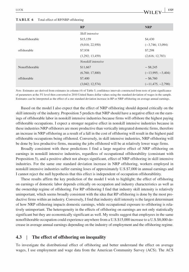
| 1325LUCK

Based on the model I also expect that the effect of NRP offshoring should depend critically on the skill intensity of the industry. Proposition 5 predicts that NRP should have a negative effect on the earn-ings of offshorable labor in nonskill intensive industries because firms will offshore the highest paying offshorable occupations. I expect a stronger negative effect in nonskill intensive industries because in these industries NRP offshorers are more productive than vertically integrated domestic firms, therefore an increase in NRP offshoring as a result of a fall in the cost of offshoring will result in the highest paid offshorable occupations being offshored. Conversely, in skill intensive industries, NRP offshoring will be done by less productive firms, meaning the jobs offshored will be at relatively lower wage firms.

Broadly consistent with these predictions I find a large negative effect of NRP offshoring on earnings in nonskill intensive industries, regardless of occupational offshorability (consistant with Proposition 5), and a positive albeit not always significant, effect of NRP offshoring in skill intensive industries. For the same one standard deviation increase in NRP offshoring, workers employed in nonskill intensive industries suffer earning loses of approximately U.S.$7,000 in annual earnings and I cannot reject the null hypothesis that this effect is independent of occupation offshorablitity.

These results affirm the key prediction of the model I wish to highlight; the effect of offshoring on earnings of domestic labor depends critically on occupation and industry characteristics as well as the ownership regime of offshoring. For RP offshoring I find that industry skill intensity is relatively unimportant, which seems broadly consistent with the idea that RP offshoring is done by the most pro-ductive firms within an industry. Conversely, I find that industry skill intensity is the largest determinant of how NRP offshoring impacts domestic earnings, while occupational exposure to offshoring is rela-tively unimportant. The heterogeneity in the effects of offshoring on earnings are not only statistically significant but they are economically significant as well. My results suggest that employees in the same nonoffshorable occupation could experience anywhere from a U.S.$15,000 increase to a U.S.$8,000 de-crease in average annual earnings depending on the industry of employment and the offshoring regime.

4.3 | The effect of offshoring on inequalityTo investigate the distributional effect of offshoring and better understand the effect on average wages, I use employment and wage data from the American Community Survey (ACS). The ACS

T A B L E 6 Total effect of RP/NRP offshoring

RP NRP

Skill intensive

Nonoffshorable $15,159 $4,430

(9,018; 22,950) (−3,746; 13,094)

offshorable $7,938 $7,298

(3,292; 13,459) (2,616; 12,783)

Nonskill intensive

Nonoffshorable $11,667 − $8,245

(6,760; 17,880) (−13,995; −3,404)

offshorable $7,400 − $6,760

(3,042; 12,574) (−11,475, −2,790)

Note. Estimates are derived from estimates in column (4) of Table 5, confidence intervals constructed from tests of joint significance of parameters at the 5% level then converted to 2010 United States dollar values using the standard deviation of wages in the sample. Estimates can be interpreted as the effect of a one standard deviation increase in RP or NRP offshoring on average annual earnings.

1326 | LUCK

provides industry codes that are based on but not directly comparable to NAICS industry classifica-tions. The theoretical model implies that changes in offshoring costs will impact the industry specific earning distribution. So, when the model predicts that a reduction in the cost of RP offshoring will increase wages among the most productive firms within an industry, this implies that wages at the top end of the industry specific wage distribution will increase. Whereas a reduction in the cost of NRP offshoring will increase wages among less productive firms, having a larger effect on the middle of the wage distribution.

To test the distributional effects of RP and NPR offshoring I implement a difference in difference model by comparing the changes over time in the real earnings distribution for industries that experi-ence large vs. small predicted changes in offshoring. Selection of treatment and control industries is done by first regressing United States RP/NRP offshoring on the full instrument set, then predicting United States offshoring. From the predicted offshoring measures, I construct the average annual change in predicted offshoring for each industry. I define industries as treated by a large offshoring shock if their average year on year growth rates in offshoring are at or above the 75th percentile across all industries, while control industries are those below the 25th percentile.44 Having defined a treat-ment and control group I estimate the impact of RP offshoring on segments of the wage distribution as follows,

empg

it∕empit is defined as the share of industry i’s employment that falls in a range of the income dis-

tribution denoted by g. To define g, I split each industry’s employment distribution into three groups corresponding to high‐, medium‐ or low‐income groups.45 TRP, i and TNRP, i are indicator variables that are equal to one for industries treated by RP and NRP offshoring shocks respectively, and Pt is an indicator variable equal to one in the post period. Disregarding intermediate years, I define 2002, 2003, and 2004 as the pretreatment period and 2009, 2010, and 2011 as the post period. Equation 26 represents a difference in difference estimator where �1 measures the impact of being treated by RP offshoring treatment without being treated by NRP offshoring, while �2 is the marginal effect of being treated by both shocks. The co-efficient of interest is �1. I estimate the model separately for offshorable and nonoffshorable occupations.

The inclusion of the interaction allows me to estimate the effect of RP offshoring treatment con-trolling for the NRP treatment. This is not a standard triple‐difference estimator because the addition of the interaction does not provide an additional control group, the control group being those indus-tries with a low RP offshoring treatment regardless of the NRP treatment.46 To estimate the effect of NRP offshoring shocks I separately construct treatment and control groups based on industry ex-posure to NRP offshoring and once again estimate Equation 26, where here I will identify the effect of a NRP treatment controlling for any RP treatment. Table 7 reports results for both RP and NRP offshoring shocks with and without the interaction terms and estimated separately for offshorable and nonoffshorable occupations. I focus on the results from the model including the interaction term since this accounts for the industries that experience both RP and NRP shocks.

The top panel reports the effect of RP offshoring treatment. For offshorable occupations I find that RP offshoring reduces high‐ and middle‐income employment and appears to shift employment to the low‐income group. This is consistent with the hypothesis that if RP offshoring is done at the expense of domestic labor, the jobs lost will be relatively high wage. For nonoffshorable occupations I find RP offshoring has the opposite effect, reducing the share of workers in the low‐ and medium‐income groups and increasing the share of workers in the high‐income group. Again, this is consistent with

(26)ln (empg

it∕empit)=�+�1TRP,i+�2TRP,i ∗TNRP,i+�3Pt +�1TRP,i ∗Pt +�2TRP,i ∗TNRP,i ∗Pt +�it.

| 1327LUCK

TA

BL

E 7

Ef

fect

of R

P an

d N

RP

offs

horin

g on

ineq

ualit

y: D

iffer

ence

in d

iffer

ence

est

imat

ion

Offs

hora

ble

Occ

upat

ions

Non

Offs

hora

ble

Occ

upat

ions

Low

inco

me

Mid

dle

Inco

me

Hig

h In

com

eLo

w in

com

eM

iddl

e In

com

eH

igh

Inco

me

Rel

ated

Par

ty o

ff-

shor

ing

treat

men

t

TR

P,i∗

Pt

0.01

410.

0865

−0.

0024

6−

0.01

040.

0374

−0.

0082

1−

0.02

08−

0.12

4−

0.09

43−

0.06

490.

179

0.27

1∗∗

(0.0

545)

(0.0

688)

(0.0

350)

(0.0

407)

(0.0

581)

(0.0

741)

(0.1

59)

(0.1

81)

(0.0

869)

(0.0

977)

(0.1

45)

(0.1

17)

TR

P,i∗

TN

RP

,i∗

Pt

−0.

157∗

0.01

720.

0988

0.21

4−

0.06

36−

0.20

2

(0.0

800)

(0.0

419)

(0.0

877)

(0.1

98)

(0.0

956)

(0.2

37)

Obs

erva

tions

150

150

150

150

150

150

150

150

150

150

150

150

Non

rela

ted

Party

of

fsho

ring

treat

men

t

TN

RP

,i∗

Pt

−0.

0363

0.07

000.

0042

00.

0836

−0.

130∗

−0.

382∗

∗0.

269∗

0.42

7∗∗∗

−0.

115+

−0.

130

−0.

242

−0.

514∗

(0.0

499)

(0.0

902)

(0.0

458)

(0.0

877)

(0.0

749)

(0.1

39)

(0.1

42)

(0.1

51)

(0.0

805)

(0.1

12)

(0.2

03)

(0.2

93)

TR

P,i∗

TN

RP

,i∗

Pt

−0.

239+

−0.

169+

0.56

8+−

0.35

3+0.

0278

0.56

8+

(0.1

57)

(0.1

09)

(0.3

72)

(0.2

15)

(0.1

93)

(0.3

72)

Obs

erva

tions

150

150

150

150

150

150

150

150

150

150

150

150

Not

e. T

his t

able

repo

rts e

stim

ates

from

est

imat

ion

Equa

tion

26 se

para

tely

for o

ffsh

orab

le a

nd n

onof

fsho

rabl

e oc

cupa

tions

. The

dep

ende

nt v

aria

ble

is th

e ra

tio o

f the

num

ber o

f wor

kers

in a

segm

ent

of th

e w

age

dist

ribut

ion

divi

ded

by a

ll w

orke

rs e

mpl

oyed

in a

n in

dust

ry a

nd y

ear p

air.

The

coef

ficie

nt re

porte

d is

the

treat

men

t eff

ect o

f a h

igh

offs

horin

g ev

ent o

r �1 fr

om E

quat

ion

26. H

igh

shoc

k in

dust

ries a

re d

efin

ed a

s ind

ustri

es w

ith a

vera

ge y

ear o

ver y

ear g

row

th ra

tes i

n th

e R

P/N

RP

offs

horin

g in

stru

men

t at o

r abo

ve th

e 75

th p

erce

ntile

acr

oss a

ll in

dust

ries,

whi

le lo

w sh

ock

indu

strie

s are

th

ose

belo

w th

e 25

th p

erce

ntile

. I u

se b

oth

Chi

nese

RP/

NR

P ex

ports

to d

evel

oped

cou

ntrie

s and

Chi

nese

RP/

NR

P ex

ports

to th

e w

orld

less

the

Uni

ted

Stat

es to

inst

rum

ent t

reat

men

t. I f

irst r

egre

ss

Uni

ted

Stat

es R

P/N

RP

offs

horin

g on

my

inst

rum

ent s

ets t

hen

pred

ict U

nite

d St

ates

off

shor

ing.

I th

en c

onst

ruct

cha

nges

in th

ese

pred

icte

d of

fsho

ring

mea

sure

s to

sele

ct h

igh

and

low

trea

tmen

t ind

us-

tries

. Inc

ome

data

is ta

ken

from

the

Am

eric

an C

omm

unity

Sur

vey.

I ad

just

ed in

com

e by

the

CPI

to g

ener

ate

real

201

0 do

llars

. I p

ool 2

002,

200

3, a

nd 2

004

as th

e pr

e ye

ars a

nd 2

009,

201

0 an

d 20

11 a

s th

e po

st y

ears

. With

25

indu

strie

s per

yea

r I h

ave

150

tota

l obs

erva

tions

. Sta

ndar

d er

rors

are

clu

ster

ed a

t the

indu

stry

leve

l res

trict

ing

my

estim

atio

n to

onl

y 25

clu

ster

s. St

anda

rd e

rror

s in

pare

nthe

ses.

+p<

0.2

0, ∗

p<

0.1

0, ∗

∗p<

0.0

5, ∗

∗∗p<

0.0

1.

1328 | LUCK

the theory that RP offshoring should be conducted by the most productive firms, for which reduced cost of RP offshoring will enhance productivity and increase wages in nonoffshorable occupations.

The second panel reports the effect of NRP offshoring treatment. For offshorable occupations the evidence suggests that treatment causes an increase in the low‐ and middle‐income employment share at the expense of the high, and for nonoffshorable occupations there is an even larger increase in the low‐income share, this time at the expense of both the middle‐ and high‐income shares. Few estimates are statistically different from zero, however this is likely owing to the fact that I disregard the middle 50% of industries to develop cleaner treatment and control groups, therefore I am left with only 25 industries over 6 years. Additionally, because of the concern that within industry income distributions are likely highly correlated across time I cluster my standard errors at the industry level, which limits variation further. Considering the limitations of the data, I find these results encouraging.

4.4 | Extensions and robustnessMy main results demonstrate a clear difference in the effect of RP and NRP offshoring on earnings, specifically that workers in nonskill intensive industries are unable to insulate themselves from the negative effects of NRP offshoring by being employed in nonoffshorable occupations, while the gains associated with RP offshoring are much larger for nonoffshorable occupations, regardless of industry skill intensity.

In the main model I include indicator variables for occupation offshorability and industry skill in-tensity in order to identify heterogeneous average treatment effects of RP and NRP offshoring across these industry and occupation characteristics. However, the chosen cutoff to construct my binary measure of offshorability is relatively arbitrary and generous in its classification of occupations as off-shorable.47 Therefore, I also estimate my preferred specification at different cutoffs for offshorability (35%, 50% 65%, 70%, and 90%). The results are qualitatively comparable across all cutoffs and are reported in Table 8. I take this as evidence that the chosen cutoff is not driving my results and that I am largely identifying off of the ends of the distribution of offshorability.

Next, I include offshorability in the model as a continuous variable interacted with offshoring, which allows me to estimate the differential effect of offshoring across occupations and industries. As treatment now varies by industry and occupation, this specification allows me to control for occupa-tion by time and industry by time fixed effects in order to absorb common shocks within occupations and industries over time by estimating the following model,

where offablecj and HSc

it are continuous variables and �jt and �it occupation by time and industry by time

fixed effects. Rather than identifying the direct effect of offshoring on wages, this strategy identifies whether these effects vary by occupation exposure to offshoring, as measure by offshorability, as well as industry skill intensity. Results are reported in Table 9 and they are broadly consistent with the main findings. The effect of RP offshoring on earnings depends heavily on occupation offshorability, whereas the effect of NRP offshoring appears to be independent offshorability before controlling for skill intensity. Isolating how industry offshoring differentially affects occupations depending on

(27)

earningsijt =�0+�1RPit ×offablecj+�2NRPit ×offablec

j

+�3RPit ×offablecj×HSc

it+�4NRPit ×offablec

j×HSc

it

+�j+�i+�jt +�it +�ijt,

| 1329LUCK

their level of exposure to offshorability is important for two reasons, first it confirms the findings of Ebenstein et al. (2014) that occupational exposure to offshoring is associated with effects on earnings, and second by controlling for common shocks within industries and occupations and over time, it reaffirms the importance in industry‐level offshoring exposure on earnings.

The results suggest the possibility of heterogeneity in the effect of offshoring across industries, to further examine this possibility I also estimate Equation 25 allowing for the marginal effect of

T A B L E 8 Effect of related and nonrelated party offshoring on average wages for alternative offshorability cutoffs

35% Offable 50% Offable 65% Offable 70% Offable 90% Offable

RP .384∗∗∗ .397∗∗∗ .418∗∗∗ 0.423∗∗∗ .492∗∗∗

(0.0841) (0.121) (0.0885) (0.105) (0.127)

NRP −0.241∗∗ −0.287∗∗ −0.119 ∗∗∗ −0.296∗∗∗ −0.385∗∗∗

(0.0713) (0.141) (0.0771) (0.100) (0.124)

RP*offble −0.369∗∗∗ −0.324∗∗ −0.260∗∗∗ −0.159∗∗∗ −0.142∗∗∗

(0.0316) (0.0495) (0.0495) (0.0439) (0.0264)

NRP*offble 0.0321 0.0042 0.0201 0.0832 0.0783

(0.0427) (0.0316) (0.0296) (0.0478) (0.0719)

RP*HS 0.092∗∗∗ 0.089* 0.108∗∗∗ 0.142∗∗∗ 0.442∗∗∗

(0.0575) (0.0399) (0.0480) (0.0213) (0.0175)

NRP*HS 0.428* 0.406 0.495∗∗ 0.592∗∗ 0.629∗∗∗

(0.243) (0.295) (0.203) (0.293) (0.144)

RP*offble*HS −0.022 −0.059∗∗ −0.093∗∗ −0.161∗∗ −0.315∗∗∗

(0.0198) (0.0202) (0.0421) (0.081) (0.0182)

NRP*offble*HS 0.0302 0.0533 0.0725 0.0901 0.0430

(0.0639) (0.0426) (0.0982) (0.0694) (0.0889)



X X X X X


X X X X X

Endogeneity p value

0.025 0.001 0.000 0.000 NA

R2 0.331 0.296 0.257 0.190 0.355

Observations 49,792 49,792 49,792 49,792 49,792

Note. The dependent variable is an occupation by industry estimate of the average wage from the OES, measured at the NAICS 4. RP and NRP are the measures of industry offshoring, offble is an indicator variable equal to one for offshorable occupations, where the percentage of occupations that are deemed offshorable varies across specifications, ranging from 35% to 90%. HS is an indicator variable equal to one for high skill industries. In the 2SLS estimation, supply‐driven change in offshoring are instrumented for using RP and NRP export from China to Europe as well as NRP exports to the world minus the United States The sample is restricted to 2002–2007 in an effort to avoid the period of highly correlated demand shocks between the United States and Europe. For all IV specifications I can reject the null hypothesis that offshoring is exogenous at the 5% level. All specifications include industry specific linear time trends along with industry, year and occupation fixed effects. Standard errors are clustered at the occupation level and reported in parentheses: *p < 0.10, ∗∗p < 0.05, ∗∗∗p < 0.01.

1330 | LUCK

T A B L E 9 Effect of RP and NRP offshoring across occupations

(1) (2) (3) (4)

RPoff × offble −0.122∗∗∗ −0.118∗∗∗ −0.121∗∗∗ −0.0705∗∗∗

(0.0125) (0.0120) (0.0123) (0.0227)

NRPoff × offble 0.00588 0.0116∗∗ 0.00530 −0.0161

(0.00403) (0.00456) (0.00395) (0.0106)

RPoff × offble × HS −0.00309∗∗

(0.00120)

NRPoff × offble × HS 0.00146∗∗

(0.000654)

Year fixed effects X X X X

Industry fixed effects X X X X

Occupation fixed effects X X X X

Industry × year fixed effects X X X

Occ × year fixed effects X X X

Exogeneity p‐value 0.000 0.000 0.000 0.000

R2 0.949 0.946 0.950 0.950

Observations 49792 49792 49792 49792

Note. The dependent variable is an occupation by industry estimate of the average wage from the OES, measured at the NAICS 4. RP and NRP are the measures of industry offshoring, offble and HS are now continuous variables with higher values indicating more offshorable occupations and more skill intensive industries respectively. In the 2SLS estimation, supply‐driven change in offshoring are instrumented for using RP and NRP export from China to Europe as well as NRP exports to the world minus the United States The sample is restricted to 2002–2007. For all IV specifications I can reject the null hypothesis that offshoring is exogenous at the 5% level. Standard errors are clustered at the occupation level and reported in parentheses: *p < 0.10, ∗∗p < 0.05, ∗∗∗p < 0.01.

F I G U R E 5 Industry specific marginal effects of offshoring. Note. The first two panels of the above figure plot the kernel densities of the marginal effects of a one standard deviation change in RP and NRP offshoring on average wages of offshorable and nonoffshorable occupations, allowing for differential effects across industries. All estimates are for our baseline cutoff of offshorability with 85% of occupations designated as offshorable respectively. The third panel plots the RP and NRP marginal effect jointly by industry in a scatter plot. This panel demonstrates the negative correlation between the marginal effect of RP and NRP offshoring in most industries [Colour figure can be viewed at wileyonlinelibrary.com]

0.2

.4.6

.8D

ensi

ty

-3 -2 -1 0 1 2 3Effect of offshoring on wages for non-offshorable occupations

RP offshoring NRP offshoring

Non-Offshorable

0.5

11.

52

Den

sity

-3 -2 -1 0 1 2 3Effect of offshoring on wages for offshorable occupations

RP offshoring NRP offshoring

Offshorable

www.wileyonlinelibrary.com

| 1331LUCK

offshoring to be heterogeneous across all industries. I plot the effects of RP and NRP offshoring on offshorable and nonoffshorable occupations in the top two panels of Figure 5. While there is substan-tial dispersion of coefficients, I estimate Kolmogorov–Smirnov tests for statistical dominance and find that the distribution of NRP coefficients is stochastically dominated by the RP coefficients for both offshorable and nonoffshorable occupations. This indicates that even though there is variation in the marginal effects of offshoring by industry, the overall results are consistent with what I capture in my main results.

5 | CONCLUSION

In this paper I propose a relationship between labor market frictions and both the location and inter-nalization decisions of firms. To motivate how these frictions affect domestic labor I develop a model that explains how match specific workforce heterogeneity, along with firm productivity heterogene-ity, leads to firms hiring labor forces with different average skill and provides incentives for firms to take on different organizational forms and source from different locations. The ability of a firm to accurately screen employee quality is limited under outsourced production, which incentivizes vertical integration, moreover the cost of filling vacancies is higher domestically, which incentivizes offshoring. From these two mechanisms I build a model of outsourcing and offshoring driven entirely by labor market frictions.

One of the key predictions of this model is that the effect of offshoring on domestic labor depends critically on the type of occupation (offshorable or not), the type of industry (skill intensive or not) and the type of offshoring (related party or nonrelated party). I rely on plausibly exogenous variation in the cost of related party and nonrelated party trade to test the predictions of my model empirically and I find evidence that supports these predictions. The results are consistent with previous studies, demonstrating that occupation characteristics are critically important to determining how offshoring effects labor, and additionally by separately identifying the effects of related party vs. nonrelated party trade I show that the impact of offshoring on labor markets also critically depends on industry skill intensity and firm organizational form.

I find that related party offshoring has a large and positive effect on earnings of those employed in nonoffshorable occupations, while having a smaller yet still positive effect on earnings of those employed in offshorable occupations. This difference across occupations appears to be independent of industry skill intensity. I find that nonrelated party offshoring has a substantial negative effect on earning of those employed in nonskill intensive industries, yet this is independent of the occupation in which a worker is employed. My estimates are both statistically and economically significant; a one standard deviation increase in related party offshoring is predicted to increase annual earnings by as much as U.S.$15,000, while a one standard deviation increase in nonrelated party offshoring is predicted to decrease earnings by as much as U.S.$8,000.

I also find evidence to suggest that offshoring not only affects average wages but also affects wage inequality by differentially affecting workers at different points on the income distribution. Related party offshoring tends to increase employment in high‐income occupations, while nonrelated party offshoring tends to have the opposite effect–removing high‐income occupations and replacing them with low‐income occupations. All of the above suggests a role for the global value chain in explaining current trends in domestic labor markets, and that when evaluating the effect of offshoring on domes-tic labor, ownership, industry, and occupation characteristics should all be considered.

1332 | LUCK

ACKNOWLEDGMENTS

Special thanks to Robert Feenstra, Katheryn Russ and Deborah Swenson for their helpful com-ments from a very early stage. I was also greatly aided by helpful comments from Giovanni Peri, Ina Simonovska, Thanasis Geromichalos as well as seminar participants at Clemson University, Colorado State University, Drexel University, Kansas City Federal Reserve, U.S. Census Center for Economic Studies, and the Midwest International Trade Meetings. Comments and suggestions provided at the Western Economic Association International’s annual meetings by Ellis Tallman, Daniel Grodzicki, Jacopo Magnani, Alvaro Pedraza and Qi Sun were also extremely helpful. As always, all errors are my own.

ENDNOTES1 Author’s calculations based on United States imports of goods with BEA end‐use classifications designated as intermedi-

ates by Wright (2014). 2 Intra‐firm imports are measured from the Related Party Trade Statistics published by the United States Census Bureau

Intra‐firm trade is defined as trade between two parties where one party holds at least a 6% ownership stake in the other. 3 This contributes to the growing literature focusing on the link between firm performance and wages (Verhoogen, 2008;

Yeaple, 2005; Bustos, 2011; Helpman, Itskhoki, & Redding, 2010b). 4 See Duhigg and Bradsher (2012). 5 Evidence that source country labor market frictions affect trade patterns has been presented by both Javorcik and

Spatareanu (2005) and Cunat and Melitz (2012). Javorcik and Spatareanu (2005) demonstrate that flexibility in the host country’s labor market in absolute terms or relative to that in the investor’s home country is associated with larger FDI inflows. Also Cunat and Melitz (2012) find that flexible labor markets can be a source of comparative advantage: countries with more flexible labor markets export more in sectors with volatile labor demand. I also provide additional supporting evidence based on the period under investigation in this paper in Online Appendix I.3 (for access to the Online Appendix see Supporting Information at the end of the paper).

6 Recently Oldenski (2012) has shown that task complexity can play an important role in determining the location of pro-duction: more routine tasks are offshored by multinationals, while the less routine are more likely to be performed at the headquarters of the multinational. Additionally Costinot, Oldenski, and Rauch (2009) find that industries with more routine employment tend to have less related party trade. Using a similar methodology to Costinot et al. (2009). and using my sample and measure of skill, I provide additional supporting evidence in Online Appendix I.3 (see Supporting Information).

7 All earnings are reported in 2010 U.S. dollars. 8 Ebenstein et al. (2014) show that offshoring to low wage countries is associated with declining wages domestically and that

these effects are concentrated on workers performing routine tasks, highlighting the importance of a worker’s occupation in determining the effect of offshoring.

9 To motivate the model I develop two stylized facts regarding labor markets and trade. The first is that labor market frictions play a role in directing FDI, and trade more generally. The second is that the skill intensity of an industry’s employment is highly correlated with it share of related party trade. These facts are developed in Online Appendix I.3 (see Supporting Information).

10 The model has a continuum of firms all of which employ a measure of workers, where each firm’s labor force has positive mass. The measurability of the labor force under this assumption is not trivial, however Duffie and Sun (2012) demonstrate the sufficient conditions for a law of large numbers to exist in such an environment, which my model meets through pair-wise independence of all matches.

11 Agents are free to search in any one of three labor markets, X, H and G, therefore the expected wage in all labor markets must be equal. Given the assumption of constant returns in the X sector, the expected wage (E[wi] = �i) must satisfy the following: wX = �h = �g. I will make this more explicit in Section 2.9.

| 1333LUCK

12 Writing costs in this way relies on assuming that that the distribution of skill is the same across labor markets. One way of extending this model would be to allow for the minimum skill to differ across countries. The cost of screening would then need to be relative to the minimum skill, one such parameterization would be the following: j = C∕�

(�c, i∕�

j

min

)�

, where �

j

min differs by country j. The role of the distribution of worker skill as a source of comparative advantage has recently been

studied by Bombardini, Gallipoli, and Pupato (2012). When skill has differential importance across industries, differences in source country skill distributions may play an important role in sourcing decisions, I will leave this for future work.

13 This is an assumption made for simplicity. In reality if this was a dynamic model, the return of being unemployed should be given by the asset value of future employment and any additional unemployment benefits. The method for making this type of model dynamic has been developed by Helpman and Itskhoki (2009).

14 See Section 2.1.3 in the Online Appendix (Suporting Information) for details. This result is also shown in the technical appendix to Helpman et al. (2010a).

15 For additional discussion of these first‐order conditions please see the the online Appendix II.1.2 (see Supporting Information at the end of the paper).

16 Γ1 is given by Γ1 = 1−(

�−1

�

) [(�−�gk)(1−�)

�+

(1−�hk)�

�+ ��h + (1−�)�g

]. Placing restrictions on parameters such that Γ1 > 0

ensures that revenue, matching and screening are all increasing in productivity. KV is given by KV ≡ (�min)�hk� + �gk(1−�)�

�g(1−�)

g ��h�

h

(k

k−1

)� + �(1−�)

×((1−�hk)�

)(1−�hk)�

�[(�−�gk)(1−�)

](�−�gk)(1−�)

� ×[(

�−1

�

)1

(1+�h +�g)

]Γ1−1

and is strictly positive, and is decreasing in both matching and screening costs.

17 A complete derivation of the firms profit function as well as expressions for the firm’s optimal choices of variables (�c, h, �c, g, mh and mg) can be found in the Online Appendix (see Supporting Information).

18 In order to highlight the mechanics of interest, it is assumed that G is specific to the final good producing firm and there do not exist any contracting frictions between the two firms. As a result the independent intermediate good producer will face a downward sloping demand and will choose Pg in order to maximize profits.

19 Under outsourced production, K is given by the following:

20 The different bargaining structure occurs because the independent intermediate goods producer only bargains with produc-

tion workers, where as a vertically integrated firm bargains with both types of labor simultaneously. 21 Under the assumptions on parameters in this paper ∂Λ/∂ λ >0, therefore as skill intensity becomes more important in G

production (an increase in λ). Intuitively, this means that the more important skill is in the production of G, the less produc-tive outsourcing becomes. Comparing Γ2 to Γ1, which govern the revenue share of the firm under outsourced production vs. vertical integration, it follows that Γ1 < Γ2 if λ is greater than δ, however, this condition can be met so long as the following holds: (𝜆−𝛽gk)∕𝛿 > 1−𝛽g. Recall that δ governs the curvature of the cost of screening and δ is assumed to be greater than 1. If this condition holds it ensures that a vertically integrated firm will spend more on screening and matching than an outsourcing firm will pay for its outsourced intermediates.

22 In the Online Appendix (see Supporting Information) I solve for all firm specific variables and show explicitly that match-ing, screening and wages are all increasing in productivity.

23 The assumption that vertical integration, both domestic and foreign, carries a higher fixed cost is constituent with the previ-ous literature and is reasonable given that vertical integration requires the ownership and operation of additional production facilities. However, I will take no definitive stance on the relative size of fixed costs for domestic vertical integration vs. offshore outsourcing. Instead I will assume that the size of these fixed costs is such that both types of production exist in equilibrium. This assumption is somewhat nonstandard; however I believe it is is empirically justified by the fact that for essentially every imported good, there exists at least some intra‐ and inter‐firm imports (Antràs & Yeaple, 2014).

24 I could also assume that the cost of opening vacancies in the foreign country (�∗O) is lower than the cost of opening vacancies

at home. This is not especially desirable, because it could be seen as ad hoc. Recall that owing to the assumptions on the matching function the cost to a firm of attaining mg matches is given by bgmg where bg is increasing in the cost of opening a

KO ≡ (�min)�hk�+�gk(1−�)��g(1−�)

g ��h�

h

(k

k−1

)�+�(1−�)

×((1−�hk)�

)(1−�hk)�

�[(�−�gk)(1−�)

](�−�gk)(1−�)

�

×

[(�−1

�

)1

(1+�h)

]�h�+(1−�hk)

× (1−�)�(1−�)

[(�−1

�

)2 1

(1+�h)(1+�g)

](1−�)(�g+(�−�gk)∕�)

.

1334 | LUCK

vacancy. Therefore, if 𝜓∗0< 𝜓0 then b∗

g< bg even if � = �∗. However, to make the model a true general equilibrium model

by removing the X sector, I would need a different mechanism to make b∗ < b. 25 In equilibrium, after bargaining, offshorers will pay lower wages to labor employed in the foreign country, however this

should not be seen as the incentive to offshore production since wages are determined through the exact same bargaining process used in the domestic labor market. Lower wages are instead an artifact of decreasing returns to hiring labor. With lower costs of opening vacancies, firms will endogenously open more vacancies, match with and hire more workers, driv-ing down each worker’s marginal product.

26 The only difference between KV and K∗V is the inclusion of the iceberg trade costs (1+t), which is also included in �∗

V.

27 While it is a strong assumption that foreign labor is identical in its match specific skill as domestic workers, it is an assump-tion that can be easily relaxed, so long as the differences in match specific quality are linear. Consider introducing a differ-ent match rate such that some fraction of foreign workers �f are not a successful match with the offshoring firm. Assuming that the screening cost is unchanged, the average skill of the workforce would be given by �̄� = (1−𝜇f )

k𝛼c, g

k−1. So long as pro-

ductivity in the X sector is sufficiently low relative to �f , offshoring is still supported in equilibrium. The condition that provides for vertically integrated offshoring in equilibrium in this case is

[(1+ t)

(1−𝜇f )𝜆

](1−𝛾)

<(

1

𝜐

)(1−𝜓2)𝛽g. 28 Once again, the only difference between KO and K∗

O is the inclusion of the iceberg trade costs (1 + t).

29 These two conditions are restatements of Equation 14 Proposition 3, which detail the necessary conditions for all four sourcing patterns to exist in equilibrium.

30 As the foreign country becomes more productive in the X sector, υ becomes closer to 1, and it becomes more difficult for this condition to be met. Intuitively, this is because as the two countries’ X sectors become more similar, so do the labor market conditions for all sectors X, H, and G. As the foreign country becomes more productive, which eliminates the ad-vantage of offshoring.

31 It should be once again noted that I do not assume that the relative size of fixed costs for domestic vertical integration vs. offshore outsourcing is identical for all industries. Instead, I will assume that the size of these fixed costs is such that both types of production exist in equilibrium. This assumption is somewhat non‐standard; however I believe it is is empirically justified by the fact that for essentially every imported good, there exists at least some intra‐ and inter‐firm imports (Antràs & Yeaple, 2014).

32 In principle RPoff it, NRPoff it should sum to total offshoring (off it) but because some trade flows are not reported as either RP or NRP, this is not always the case. However, these nondesignated flows are a very small minority of total flows, less than 2% on average. Summary statistics for and additional information about the construction of these measures can be found in the Online Appendix (see Supporting Information).

33 These measures impose a stricter comparability assumption than the traditional Feenstra–Hanson measure requiring that each industry i’s purchases of imported intermediates from industry k mirrors the economy‐wide intra‐firm import share of purchases in industry k. This measure of offshoring assumes that the economy‐wide import share of intermediate consumption in an industry k is the same as the import share of intermediates purchased by industry i. To compute the purchases of inputs by industry i from industry k, I start with the 2002 BEA detailed use input–output table, which details the value of inputs purchased by each industry from other industries.

34 A similar methodology has recently been employed by Acemoglu, Autor, Hanson, and Price (2016) to investigate the ef-fects of Chinese import competition through supply chain linkages. The authors do not explicitly consider their measure of downstream import competition as a proxy for offshoring but it has many similarities. The largest difference between their first‐order measure and mine is the fact that since I am interested in offshoring specifically I restrict input–output linkages to the same NAICS‐3 industry group, as discussed earlier.

35 I use foreign ownership as a proxy for related party offshoring but clearly foreign owned firms need not trade with their par-ent firm. This metric has been used in the past by Feenstra and Hanson (2005), Feenstra, Hong, Ma, and Spencer (2013), and Fernandes and Tang (2012).

36 This instrument is similar to the methodology of Autor et al. (2013) and I use the same set of countries as well. In combina-tion they mirror United States levels of imports from China well. The countries are Australia, Denmark, Finland, Germany, Japan, New Zealand, Spain, and Switzerland.

37 This instrument is similar to the one used by Hummels et al. (2014). I do not use a ROW instrument for RP offshoring as it is far less likely that exports from foreign‐owned firms in China are truly intra‐firm transaction for all countries, especially other developing countries.

| 1335LUCK

38 O*NET provides detailed descriptions of the tasks, activities, and mental and physical requirements of over 800 occupa-tions. A binary measure of occupation offshorability and skill intensity are constructed by first constructing a continuous measure similar to that suggested by Firpo, Lemieux, and Fortin (2011) and refined by Autor and Dorn (2013), then choosing a cutoff level across the distribution of occupations. I utilize five specific activities described for each occupation, to classify an occupation as highly nonoffshorable. These activities are: (1) establishing and maintaining personal relation-ships, (2) assisting and caring for others, (3) performing for or working directly with the public, (4) selling to or influencing others, and (5) communicating with supervisors, peers, or subordinates. For more information about the construction of this measure see Online Appendix I.1.4 (see Supporting Information for access).

39 This is a higher share of offshorable employment than would be suggested by Blinder and Krueger (2013), who argue that 20% to 30% of employment is offshorable. I prefer to err on the side of considering more occupations offshorable in order to allow for treatment effects on occupations for which even a small portion of the tasks they perform may be offshored. However, I will show in Section 4.4 that my results are robust to altering this threshold. For additional information about the construction and justification of this measure, see Online Appendix I.1.4 (see Supporting Information).

40 The data originated from the Orbis database. I employ the measure that is calculated as the natural log of global R&D expenditures divided by firm sales in each industry.

41 Under the assumption that wages are a function of offshoring costs (the effect of NRP being negative and RP being posi-tive) and the level of demand (the effect of demand on wages being positive), OLS is expected to generate a bias that will attenuate results for both RP and NRP offshoring. This bias comes from two sources: (1) measurement error as observed offshoring is an imprecise measure of the cost of offshoring, and (2) a correlation with the error term, which includes de-mand shocks. For a more complete discussion of this bias as well as full OLS results, see Online Appendix Section I.4.1.2 for details (see Supporting Information for access).

42 Earnings are reported in 2010 real U.S. dollars. 43 For a complete OLS estimates of Equation 25 see the Online Appendix(for access, see Supporting Information).. Estimates

in Table 6 are derived from estimates in Table 5. This table reports the implied change in averages earnings caused by a one standard deviation increase in either RP or NRP offshoring for workers depending on occupation and industry characteris-tics. P values are derived from tests of joint significance of parameters and dollar values are computed using the standard deviation of earnings in the sample. The standard deviation of earnings is U.S.$25,607.

44 I use both Chinese RP/NRP exports to developed countries and Chinese RP/NRP exports to the world less the United States to instrument treatment. I first regress United States RP/NRP offshoring on the instrument set then predict United States offshoring, then construct changes in these predicted offshoring measures to select high and low treatment industries.

45 I compute income percentiles separately for each industry from the 2002 ACS. High income is defined as the 70th through 99th percentile of wages. Medium is defined as the 35th through the 70th percentile of wages and low is defined as the 5th through the 35th percentile.

46 The control group can be thought of as all industries with low RP offshoring shocks, which can be split into three sub-groups depending on their level of NRP treatment: those only in the RP control group, those who are also in the control group for the NRP shock, and those in the NRP treatment group.

47 Blinder and Krueger (2013) estimate that approximately 30% of United States employment is offshorable. The measure used by Blinder and Krueger (2013) is not directly comparable to that used in this paper because my measure is based on the share of occupations rather than those occupations’ employment shares. Converting my 85% of occupations to their employment share produces a slightly lower employment share of 68%. That is clearly still substantially higher than the estimate of Blinder and Krueger (2013), however, I believe my measure is reasonable for three reasons: (1) my estimates are not overly sensitive to reducing this cutoff, (2) my measure of offshorability is based on the measure developed Firpo, Lemieux, and Fortin (2011) and differs from the measure proposed by Blinder and Krueger (2013), and by this measure, occupations below the median of offshorability level remain considerably offshorable (e.g., by my estimates the median occupation is “Tool grinders, filers and sharpeners”), and (3) I am interested in a broad measure of offshorability such that I consider an occupation offshorable even if only some tasks performed by that occupation are in fact offshorable. For additional details on my measure of offshorability and how it compares to the literature, see Online Appendix I.1.4 (for access, see Supporting Information).

1336 | LUCK

REFERENCES

Abowd, J. M., Kramarz, F., & Margolis, D. N. (1999). High wage workers and high wage firms. Econometrica, 67(2), 251–334.

Acemoglu, D., Autor, D., Dorn, D., Hanson, G. H., & Price, B. (2016). Import Competition and the Great US Employment Sag of the 2000s. Journal of Labor Economics, 34(S1), 141–198.

Amiti, M., & Davis, D. R. (2012). Trade, firms, and wages: Theory and evidence. Review of Economic Studies, 79(1), 1–36.

Antràs, P., & Chor, D. (2012). Organizing the Global Value Chain. Working Paper 18163, Cambridge, MA: National Bureau of Economic Research.

Antràs, P., & Chor, D. (2013) Organizing the global value chain. Econometrica, 81(6), 2127–2204.Antràs, P., & Helpman, E. (2004). Global sourcing. Journal of Political Economy, 112(3), 552–580.Antràs, P., & Helpman, E. (2006). Contractual frictions and global sourcing. Working Paper 12747, Cambridge, MA:

National Bureau of Economic Research.Antràs, P., & Yeaple, S. (2014). Multinational firms and the structure of international trade. In G. Gopinath, E. Helpman,

& K. Rogoff (Eds.), Handbook of international economics (Vol. 4, chap. 2, pp. 55–130). Amsterdam: Elsevier.Autor, D. H., & Dorn, D. (2013). The Growth of Low-Skill Service Jobs and the Polarization of the US Labor Market.

American Economic Review, 103(5), 1553–1597.Autor, D. H., Dorn, D., & Hanson, G. H. (2013). The China syndrome: Local labor market effects of import competition

in the U.S. American Economic Review, 103(6), 2121–2168.Blinder, A. S. (2007). How many U.S. jobs might be offshorable? Working Papers 60, Princeton, NJ: Princeton

University, Department of Economics, Center for Economic Policy Studies.Blinder, A. S., & Krueger, A. B. (2013). Alternative Measures of Offshorability: A Survey Approach. Journal of Labor

Economics, 31(S1), S97–S128.Bombardini, M., Gallipoli, G., & Pupato, G. (2012). Skill dispersion and trade flows. American Economic Review,

102(5), 2327–2348.Broda, C., & Weinstein, D. E. (2006). Globalization and the gains from variety. The Quarterly Journal of Economics,

121(2), 541–585.Bustos, P. (2011). The impact of trade liberalization on skill upgrading evidence from Argentina. Working Papers 559,

Barcelona, Spain: Barcelona Graduate School of Economics.Cameron, A. C., Gelbach, J. B., & Miller, D. L. (2011). Robust inference with multiway clustering. Journal of Business

& Economic Statistics, 29(2), 238–249.Costinot, A., Oldenski, L., & Rauch, J. E. (2009). Adaptation and the boundary of multinational firms. Working Paper

14668, National Bureau of Economic Research.Cunat, A., & Melitz, M. J. (2012). Volatility, labor market flexibility, and the pattern of comparative advantage. Journal

of the European Economic Association, 10(2), 225–254.Davidson, C., Martin, L., & Matusz, S. (1999). Trade and search generated unemployment. Journal of International

Economics, 48(2), 271–299.Duffie, D., & Sun, Y. (2012) The exact law of large numbers for independent random matching. Journal of Economic

Theory, 147(3), 1105–1139.Duhigg, C., & Bradsher, K. (2012, January 21). How the US lost out on iPhone work. New York Times.Durbin, J. (1954) Errors in variables. Review of the International Statistical Institute, 22(1/3), 23–32.Ebenstein, A., Harrison, A., McMillan, M., & Phillips, S. (2014). Estimating the impact of trade and offshoring on

American workers using the current population surveys. The Review of Economics and Statistics, 96(4), 581–595.Feenstra, R., & Hanson, G. (1996). Globalization, Outsourcing, and Wage Inequality. American Economic Review,

86(2), 240–245.Feenstra, R. C., & Hanson, G. H. (1999). The impact of outsourcing and high‐technology capital on wages: Estimates

for the U.S., 1979–1990. The Quarterly Journal of Economics, 114(3), 907–940.Feenstra, R. C., & Hanson, G. H. & Hanson, G. H. (2005). Ownership and control in outsourcing to China: Estimating

the property‐rights theory of the firm. The Quarterly Journal of Economics, 120(2), 729–761.Feenstra, R. C., Hong, C., Ma, H., & Spencer, B. J. (2013). Contractual versus non‐contractual trade: The role of insti-

tutions in China. Journal of Economic Behavior & Organization, 94(C), 281–294.

| 1337LUCK

Fernandes, A. P., & Tang, H. (2012). Determinants of vertical integration in export processing: Theory and evidence from China. Journal of Development Economics, 99(2), 396–414.

Firpo, S., Lemieux, T., & Fortin, N. (2011). Decomposition Methods in Economics. In D. Card & O. Ashenfelter (Eds.), Handbook of Labor Economics, 4th edition (pp. 1–102). North Holland: Elsevier.

Geishecker, I. (2006). Does outsourcing to central and Eastern Europe really threaten manual workers’ jobs in Germany? The World Economy, 29(5), 559–583.

Grossman, S. J., & Hart, O. D. (1986) The costs and benefits of ownership: A theory of vertical and lateral integration. Journal of Political Economy, 94(4), 691–719.

Hausman, J. A. (1978) Specification Tests in Econometrics. Econometrica, 46(6), 1251–1271.Helpman, E., & Itskhoki, O. (2009). Labor market rigidities, trade and unemployment: A dynamic model. (Working

Paper). Cambridge, MA: Harvard University.Helpman, E., & Itskhoki, O. (2010) Labour market rigidities, trade and unemployment. Review of Economic Studies,

77(3), 1100–1137.Helpman, E., Itskhoki, O., & Redding, S. (2010a). Inequality and unemployment in a global economy. Econometrica,

78, 1239–1283.Helpman, E., Itskhoki, O., & Redding, S. (2010b) Unequal effect of trade on workers with different abilities. Journal of

the European Economic Association, 8(2–3), 421–433Hummels, D., Jorgensen, R., Munch, J., & Xiang, C. (2014) The wage effects of offshoring: evidence from Danish

Matched worker–firm data. American Economic Review, 104(6), 1597–1629.Irarrazabal, A., Moxnes, A., & Ulltveit‐Moe, K. H. (2013). Heterogeneous firms or heterogeneous workers? Implications

for exporter premiums and the gains from trade. The Review of Economics and Statistics, 95(3), 839–849.Javorcik, B. S., & Spatareanu, M. (2005). Do foreign investors care about labor market regulations? Review of World

Economics, 141(3), 375–403.Jensen, J., & Kletzer, Lori G. (2010). Measuring Tradable Services and the Task Content of Offshorable Services Jobs,

pp. 309–335. Labor in the New Economy, National Bureau of Economic Research, Inc.Krishna, P., & Sethupathy, G. (2011). Trade and inequality in India. Working Paper 17257, Cambridge, MA: National

Bureau of Economic Research.Melitz, M. J. (2003). The impact of trade on intra‐industry reallocations and aggregate industry productivity.

Econometrica, 71(6), 1695–1725.Nunn, N. (2007). Relationship‐specificity, incomplete contracts, and the pattern of trade. The Quarterly Journal of

Economics, 122(2), 569–600.Nunn, N., & Trefler, D. (2008). The boundaries of the multinational firm: An empirical analysis. In D. M. H. Elhanan

& T. Verdier (Eds.), The Organizations of Firms in a Global Economy. Cambridge, MA: Harvard University Press.Nunn, N., & Trefler, D. (2013) Incomplete contracts and the boundaries of the multinational firm. Journal of Economic

Behavior & Organization, 94(C), 330–344.Oldenski, L. (2012). The task composition of offshoring by U.S. multinationals. International Economics, 131, 5–21.Ottaviano, G. I. P., Peri, G., & Wright, G. C. (2013). Immigration, offshoring, and American jobs. American Economic

Review, 103(5), 1925–1959.Rauch, J. (1999). Networks Versus Markets in International Trade. Journal of International Economics, 48, 7–35.Ruggles, S., Sobek, M., Alexander, T., Fitch, C., Goeken, R., Hall, P. K., ... Ronnander, C. (2010). Integrated Public

Use Microdata Series: Version 5.0 [Machine‐readable database] (Technical Report). Minneapolis, MN: University of Minnesota.

Silva, J. M. C. S., & Tenreyro, S. (2006). The log of gravity. The Review of Economics and Statistics, 88(4), 641–658.Silva, J. M. C. S., & Tenreyro, S. (2011). Further simulation evidence on the performance of the Poisson pseudo‐maxi-

mum likelihood estimator. Economics Letters, 112(2), 220–222.Sly, N., Oldenski, L., & Kovak, B. (2017). The labor market effects of offshoring by U.S. multinational firms: Evidence

from changes in global tax policies. Paper presented at the annual meeting of the Society for Economic Dynamics, June 2017, Edinburgh, Scotland.

Stole, L. A., & Zwiebel, J. (1996a). Intra‐firm bargaining under non‐binding contracts. Review of Economic Studies, 63(3), 375–410.

Stole, L. A., & Zwiebel, J. (1996b). Organizational design and technology choice under intrafirm bargaining. American Economic Review, 86(1), 195–222.

1338 | LUCK

Verhoogen, E. A. (2008). Trade, quality upgrading, and wage inequality in the Mexican manufacturing sector. The Quarterly Journal of Economics, 123(2), 489–530.

Voigtländer, N. (2014). Skill bias magnified: Intersectoral linkages and white‐collar labor demand in U.S. manufactur-ing. The Review of Economics and Statistics, 96(3), 495–513.

Wright, G. C. (2014). Revisiting the employment impact of offshoring. European Economic Review, 66(C), 63–83.Wu, De‐Min (July 1973). Alternative Tests of Independence between Stochastic Regressors and Disturbances.

Econometrica, 41(4), 733–750.Yeaple, S. R. (2005). A simple model of firm heterogeneity, international trade, and wages. Journal of International

Economics, 65(2), 1–20.

SUPPORTING INFORMATION

Additional supporting information may be found online in the Supporting Information section at the end of the article.

How to cite this article: Luck P. Intermediate good sourcing, wages and inequality: From theory to evidence. Rev Int Econ. 2019;27:1295–1350. https ://doi.org/10.1111/roie.12400

APPENDIX PROOF OF LEMMAS AND PROPOSITIONS

A1. Proof of Lemma 2

Lemma When worker skill is distributed Pareto, with shape parameter k and lower support αmin, for a chosen screening threshold �c, i the average skill of the workforce is given by,

Proof Since �̄� is defined as the expected value of worker skill I can define �̄�i ≡ �∞𝛼c, i

𝛼f𝛼(𝛼), where fα(α) is the probability density function of the skill distribution and is given by, f�(�) = k

(�min

k

�k+ 1

). Using the above expression for fα(α) and integrating over α I obtain the

following

Therefore, �̄�i =k𝛼c, i

(k−1), and is increasing in the chosen screening threshold �c, i.

�̄�i =k𝛼c,i

(k−1).

�̄�i =∫∞

𝛼c, i

k

(𝛼c, i

k

𝛼k

)=

k𝛼c, i

(k−1).

https://doi.org/10.1111/roie.12400

| 1339LUCK

A2. Proof of Lemma 3

Lemma The intermediate good producer will choose αc, g and mg such that the marginal revenue of the final good producing firm is equal to their own marginal cost of production. As such, all choice variables can be expressed in terms of the final good producers productivity as follows,

Proof A profit maximizing intermediate good producer, after matching with a final good producer, chooses the price, of its own good with full knowledge of the productivity of the final good producer. In addition to setting a price it also chooses a level of matching and screening to minimize cost conditional an meeting demand. In order to find the profit maximizing levels screening and matching, I must first determine demand. Consider a final good producer who is outsourcing production of G, therefore choosing αc, h, nh, and G to produce z(θ). Under the assumption that the timing of production is the same as before, but now the firm also decides on a level G before bargaining over wages, the profit function of the firm can be written as:

Maximizing with respect to the firms choice variables yields the following FOCs:

Given the above, demand for the intermediate good as a function of the price is given by D(Pg) =

(�−1)(1−�)

�(1+�h)Pg

r(�) where it can be shown that r(θ) is decreasing in Pg. Therefore, the revenue of the

intermediate producer is given by,

and is simply a constant share of the revenue of the final producer. We are ensured an interior solution due to the fact that revenue is decreasing in Pg and limPg→∞ r(�) = 0. The intermediate good producer will

mg(�)=(�−1

�

)2 (1−�)2�g

bg(1+�h)(1+�g)r(�) , �c, g(�)=

[(�−1

�

)2 (1−�)2(1−�gk)

C(1+�h)(1+�g)r(�)

]1∕�

ΠO(�) =max

[(1

1+�h

)AZ

(��om

�h�

h(�c, h)(1−�hk)�G1−�

) �−1

�

]

−(fO+C�c, h

�∕�+bhmh+G∗Pg

)

(28)(�−1)�h�

�(1+�h)r(�)=bhmh(�)

(29)(�−1)(1−�hk)�

�(1+�h)r(�)=C��

c,h

(30)(�−1)(1−�)

�(1+�h)r(�)=G∗Pg.

D(Pg)∗Pg =(�−1)(1−�)

�(1+�h)r(�)

1340 | LUCK

therefore choose Pg, αc, h and nh, such that the marginal revenue of the final good producing is equal to their own marginal cost of production.

Firms search for labor by the same method as final goods producers and therefore pay the same level of costs for filling vacancies (bg) and have access to the same screening technology as final goods producers. Once matching and screening take place firms and workers bargain to determine wages, where wages are again determined by the value marginal profit of the worker.

Using the revenue function implied by Equation (A3) wages for workers employed by intermediate goods firms are give by, wg =

�g

1+�g

r(ng)

ng

, where the firm's share of revenue is once again the remaining 1/

(1 + ϕg).48 I can then write the firms profit maximizing problem as the following,

Expressing r(θ) as a function of the intermediate producers choice variables I can express the profit func-tion as,

Taking the derivate with respect to αc, g and mg I can use the first-order conditions to solve for the optimal amount of G provided by the intermediate firm. Where the intermediate good production is given my

I can the describe G as a function of the downstream firm's revenue:

Equation (A3) along with (A4) imply that Pg is not the same across all firm pairs, since the inter-mediate firms revenue (G*Pg) and production G both are function of the downstream firms revenue, but increase with revenue at different rates. Utilizing Equations (A3) and (A4) I can solve the optimal Pg set by the intermediate producer as a function of the downstream firms own revenue.

�[r(ng)−wg(ng)ng

]�ng

=wg.

Πg =max

{(1

1+�g

)(�−1)(1−�)

�(1+�h)r(�)−

(fg+C�c, g

�∕�+bgmg

)}.

Πg(�)= maxmg,�c, g

[(1

1+�g

)(�−1)(1−�)

�(1+�h)AZ

(��om

�h�

h(�c, h)(1−�hk)�m

�g(1−�)

g ��(�c, g)(�−�gk)(1−�)) �−1

�

]

−(C�c, g

�∕�+bgmg

).

G=k��c, g

(k−1)

�

m�g

g

(�min

�c, g

)k�g

,

(31)P=�k�g

min

k�

(k−1)

�[(

�−1

�

)2 r(�)(1−�)2

(1+�h)(1+�g)

]�g+(�−k�g)

�(�g

bg

)�g(

1−�gk

C

) (�−k�g)

�

Pg = r(�)1−�g+(�−k�g)∕�

⎧⎪⎨⎪⎩�

k�g

min

k�

(k−1)

��

�−1

�

�2 (1−�)2�g

(1+�h)(1+�g)

��g⎫⎪⎬⎪⎭

−1

C(�−k�g)

� bg�g

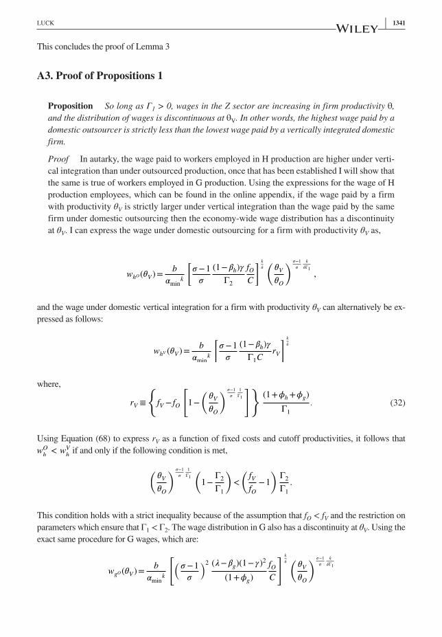
| 1341LUCK

This concludes the proof of Lemma 3

A3. Proof of Propositions 1

Proposition So long as Γ1 > 0, wages in the Z sector are increasing in firm productivity θ, and the distribution of wages is discontinuous at θV. In other words, the highest wage paid by a domestic outsourcer is strictly less than the lowest wage paid by a vertically integrated domestic firm.

Proof In autarky, the wage paid to workers employed in H production are higher under verti-cal integration than under outsourced production, once that has been established I will show that the same is true of workers employed in G production. Using the expressions for the wage of H production employees, which can be found in the online appendix, if the wage paid by a firm with productivity θV is strictly larger under vertical integration than the wage paid by the same firm under domestic outsourcing then the economy‐wide wage distribution has a discontinuity at θV. I can express the wage under domestic outsourcing for a firm with productivity θV as,

and the wage under domestic vertical integration for a firm with productivity θV can alternatively be ex-pressed as follows:

where,

Using Equation (68) to express rV as a function of fixed costs and cutoff productivities, it follows that wO

h< wV

h if and only if the following condition is met,

This condition holds with a strict inequality because of the assumption that fO < fV and the restriction on parameters which ensure that Γ1 < Γ2. The wage distribution in G also has a discontinuity at θV. Using the exact same procedure for G wages, which are:

whO (�V )=b

�mink

[�−1

�

(1−�h)�

Γ2

fO

C

] k

�(�V

�O

) �−1

�

k

�Γ1

,

whV (�V )=b

�mink

[�−1

�

(1−�h)�

Γ1CrV

] k

�

(32)rV ≡{

fV − fO

[1−

(�V

�O

) �−1

�

1

Γ1

]}(1+�h+�g)

Γ1

.

(𝜃

V

𝜃O

) 𝜎−1

𝜎

1

Γ1

(1−

Γ2

Γ1

)<

(fV

fO

−1

)Γ

2

Γ1

.

wgO (�V )=b

�mink

[(�−1

�

)2 (�−�g)(1−�)2

(1+�g)

fO

C

] k

� (�V

�O

) �−1

�

k

�Γ1

1342 | LUCK

and

Once again using the explicit equations for wages to express rUV

as a function of fixed costs and cutoff productivities, it is straightforward to show that wO

p< wV

p so long as the following condition holds,

Given that the restrictions on parameters already discussed, 𝜎−1

𝜎

1−𝛾

1+𝜙g

< 1; therefore this condition holds

trivially. This concludes the proof of Proposition 1.

A4. Proof of Propositions 3

Proposition Wages in the Z sector are increasing in firm productivity θ, and for a given level of productivity, so long as the following holds,

domestic wages are higher under vertically integrated offshoring than under domestic vertically integration.

Proof Using the expressions for the wage of H production employees I prove this proposition by demonstrating that the wage paid by a firm with productivity �̂� is strictly larger under verti-cal integration than the wage paid by the same firm under domestic vertical integration. Using expressions for headquarters wages wh(�̂�) under vertically integrated production, found in the online appendix, I have the following expression for wages under the two regimes:

Comparing these two expression allows me to derive the following inequality, which must hold for wages

under offshoring to be higher (

𝜃∗V

𝜃V

) 𝜎−1

𝜎

1

𝛿Γ1 <

(r

U, S∗

V

rS, U

V

). Without making any assumptions regarding skill

intensity, I can substitute expressions for revenue and the cutoff productivities with those derived above

and simplify this expression to, (

b∗

b

) 𝜎−1

𝜎<(

K∗V

KV

). Lastly, employing the expression for b and b* and not-

ing the only difference between K∗V and KV is the inclusion of trade costs t I can simply this expression to

the following:

wgV (�V )=b

�mink

[�−1

�

(�−�g)(1−�)

(1+�h+�g)CrV

] k

�

(𝜃V

𝜃O

) 𝜎−1

𝜎

1

Γ1

(𝜎−1

𝜎

1−𝛾

1+𝜙g

−Γ2

Γ1

)<

(fV

fO−1

)Γ2

Γ1

.

(1+ t)(1−𝛾) <(

1

𝜐

)(1−𝛽g)𝛽g

,

wh(�̂�)=

(�̂�

𝜃V

) 𝜎−1

𝜎

k

𝛿Γ1 b

𝛼mink

[𝜎−1

𝜎

(1−𝛽h)𝛾

(1+𝜙h+𝜙g)Cr

S, U

V

] k

𝛿

wh(�̂�)=

(�̂�

𝜃∗V

) 𝜎−1

𝜎

k

𝛿Γ1 b

𝛼mink

(𝜎−1

𝜎

𝛾(1−𝛽h)rS, U∗

V

(1+𝜙h+𝜙g)C

) k

𝛿

(1+ t)(1−𝛾) <(

1

𝜐

)(1−𝛽g)𝛽g

.

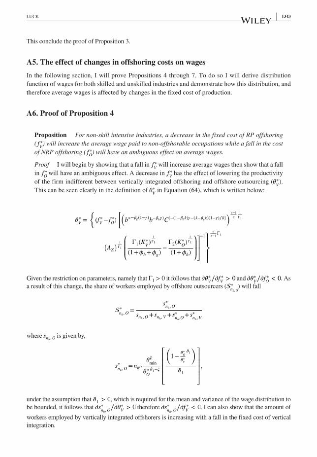
| 1343LUCK

This conclude the proof of Proposition 3.

A5. The effect of changes in offshoring costs on wagesIn the following section, I will prove Propositions 4 through 7. To do so I will derive distribution function of wages for both skilled and unskilled industries and demonstrate how this distribution, and therefore average wages is affected by changes in the fixed cost of production.

A6. Proof of Proposition 4

Proposition For non‐skill intensive industries, a decrease in the fixed cost of RP offshoring ( f ∗

V) will increase the average wage paid to non‐offshorable occupations while a fall in the cost

of NRP offshoring ( f ∗O) will have an ambiguous effect on average wages.

Proof I will begin by showing that a fall in f ∗V will increase average wages then show that a fall

in f ∗O will have an ambiguous effect. A decrease in f ∗

V has the effect of lowering the productivity

of the firm indifferent between vertically integrated offshoring and offshore outsourcing (�∗V).

This can be seen clearly in the definition of �∗V in Equation (64), which is written below:

Given the restriction on parameters, namely that Γ1 > 0 it follows that 𝜕𝜃∗V∕𝜕f ∗

V> 0 and 𝜕𝜃∗

V∕𝜕f ∗

O< 0. As

a result of this change, the share of workers employed by offshore outsourcers (∗nh, O

) will fall

where snh, O is given by,

under the assumption that 𝜗1 > 0, which is required for the mean and variance of the wage distribution to be bounded, it follows that 𝜕s∗

nh, O∕𝜕𝜃∗

V> 0 therefore 𝜕s∗

nh, O∕𝜕f ∗

V< 0. I can also show that the amount of

workers employed by vertically integrated offshorers is increasing with a fall in the fixed cost of vertical integration.

�∗V=

�(f ∗

V− f ∗

O)

��b∗−�g(1−�)

b−�h�)C[−(1−�hk)�−(�−�gk)(1−�)∕�]� �−1

�

1

Γ1

�AZ

� 1

Γ1

⎛⎜⎜⎝

Γ1(K∗V

)1

Γ1

(1+�h+�g)−Γ2(K∗

O)

1

Γ1

(1+�h)

⎞⎟⎟⎠

⎤⎥⎥⎦

−1⎫⎪⎬⎪⎭

�

�−1Γ1

∗nh, O

=s∗

nh, O

snh, O+snh, V +s∗nh,O

+s∗nh, V

s∗nh, O

=nhO

��

min

�∗O

�1−�

⎡⎢⎢⎢⎢⎣

�1−

�∗O

�∗V

�1

�

�1

⎤⎥⎥⎥⎥⎦

,

1344 | LUCK

Next, I will show that share of workers employed by vertically integrated offshorers is decreasing in �∗

V. I can derive the following expression for s∗

ng, V,

where the share of workers employed by vertically integrated offshorers is

From the above it is not as easy to see how a change in f ∗V effects s∗

nh, V, since f ∗

V effects both �∗

V and n∗

gV,

however by using the expressions for �∗V and n∗

gV derived in Equation (64) and the online appendix I can

show that

As a result, it becomes clear that s∗nh, V

is decreasing in both �∗V and f ∗

V. Additionally, the share of workers

employed by domestic firms, both outsourcing and vertically integrated firms are not affected, therefore I simply had a shift in employment toward vertically integrated offshorers, who screen more heavily and therefore pay higher wages than offshore outsourcers as have already been established in Proposition 1. This change will have an unambiguous and positive effect on the average wage of domestic employees in H sector employment.

Next I will establish that a fall in the cost of offshore outsourcing, f ∗O will have an ambiguous

effect on average wages for those employed in non‐offshorable occupations, i.e., h sector employees. A decrease in f ∗

O has the effect of lowering the productivity of the firm indifferent between domestic

vertical integration and offshore outsourcing (�∗O). This can be seen in the definition of �∗

O for non‐

skill intensive industries in the online appendix, therefore 𝜕𝜃∗O∕𝜕f ∗

O> 0. It is also clear from 64 that

𝜕𝜃∗V∕𝜕f ∗

O< 0

As a result, a decrease in f ∗O will unambiguously increase the share of workers employed by firms

engaging in offshore outsourcing (∗nh, O

), which is once again given by

where snh, O is given by,

s∗nh,V

=n∗hV

��

min

�∗V

�1−�

(�∗

V

−�1

�1

)

∗nh, V

=s∗

nh, V

snh, O+snh, V +s∗nh, O

+s∗nh, V

.

�(

n∗hV

�∗V

�1−�

)

�f ∗V

=0.

∗nh, O

=s∗

nh, O


+s∗nh, V

,

s∗n

h, O=n

hO

��

min

�∗O

�1−�

⎡⎢⎢⎢⎢⎣

�1−

�∗O

�∗V

�1

�

�1

⎤⎥⎥⎥⎥⎦

.

| 1345LUCK

This increase in the share of workers employed by offshore outsourcers will come at the expense of both domestic vertically integrated firms (because �∗

O falls) and vertically integrated offshorers (because �∗

V

rises). This can be seen clearly by observing the share of workers employed by vertically integrated firms, both foreign and domestic fall with �∗

O, by examining s∗

nh, O, and s∗

nh, V,

Recalling from above that the following conditions hold

it is clear that both shares decline when the cost of offshore outsourcing ( f ∗O) falls. Unlike the previous

case, the effect on average wages is not clear cut. Since offshore outsourcers will pay higher wages then domestic vertically integrated firms, an increase in offshore outsourcing that comes at the expense of domestic vertical integration will have the effect of increasing decreasing wages. However, since offshore outsourcers will pay lower wages then foreign vertically integrated firms, an increase in offshore outsourc-ing that comes at the expense of foreign vertical integration will have the effect of decreasing average wages. Therefore, the overall effect on average wages will be ambiguous. This concludes the proof of Proposition 1.


Proposition For non‐skill intensive industries a decrease in the fixed cost of in offshoring ( f ∗V)

will have no effect on average wage paid to offshorable occupations (G sector), while a fall in the cost of NRP offshoring ( f ∗

O) will decrease the average wage paid to offshorable occupations

(G sector).

Proof I will begin by demonstrating that a decrease in the fixed cost of in RP offshoring ( f ∗V)

will not the average wage paid to offshorable occupations in non‐skill intensive industries. The average domestic wage in the G sector is only affected by those firms who onshore production. In non‐skill intensive industries, the sorting of firms is such that offshorers are all more pro-ductive than onshorers (i.e. the productivity sorting satisfies the following 𝜃O < 𝜃V < 𝜃∗

O< 𝜃∗

V).

Therefore, as I demonstrated in the online appendix the distribution of wages in the G sector are given by,

snh,V =nhV

��

min

�V�1−�

⎡⎢⎢⎢⎣

�1−

�V

�∗O

�1�

�1

⎤⎥⎥⎥⎦

, s∗nh, V

=n∗hV

��

min

�∗V

�1−�

��∗

V

−�1

�1

�.

�(

nhV

�V�1−�

)

�f ∗O

=0, and

�(

n∗hV

�∗V

�1−�

)

�f ∗O

=0,

Gwg(w)=

⎧⎪⎪⎨⎪⎪⎩

ng,OGwg,O(w) for wgO ≤w≤wgO

��V

�O

� �−1

�

k

�Γ1 ,

ng,O for wgO

��V

�O

� �−1

�

k

�Γ1 ≤w≤wgV ,

ng,VGwg,V (w) for wgV ≤w≤wgV

��∗

O

�V

� �−1

�

k

�Γ1 ,

1346 | LUCK

The above expression for the distribution of wages in the G sector, makes clear that the distribution, and therefore the average wage, depends on underlying parameters along with the following cutoff produc-tivities: θO, θV, and �∗

O. Each cutoff can be solved for explicitly, which I detail in the online appendix, and

are given by:

and

Examining Equations (61)–(63), it is clear to see that none depend on the cost of vertically integrated off-shoring f ∗

V, and therefore a change in this cost will not affect the waged distribution or the average wage.

Alternatively consider a decrease in the cost of offshore outsourcing ( f ∗O). From equation (63), it is

clear that 𝜕𝜃∗O∕𝜕f ∗

O> 0. This has two effects, it decreases the share of workers employed by domestic

vertically integrated firms since 𝜕sng,V∕𝜕𝜃∗O> 0, and it lower the truncation point of the wage distri-

bution, which is given by wgV

(�∗

O

�V

) �−1

�

k

�Γ1. Intuitively, a fall in the cost of offshore outsourcing incen-

tives the more productive firms who are employing G sector employs domestically to offshore production thereby eliminated they highest paying G sector jobs and lowering the average wage. This concludes the proof of Proposition 5.

sng, O =ngO

��

min

��1+�

O

⎡⎢⎢⎢⎣

�1−

�O

�V

�1�

�1

⎤⎥⎥⎥⎦

, and sng, V =ngV

��

min

��1+�

V

⎡⎢⎢⎢⎣

�1−

�V

�O∗

�1�

�1

⎤⎥⎥⎥⎦

(33)�O =

⎧⎪⎨⎪⎩

Γ2(KO)1

Γ1 (AZ)1

Γ1

fO(1+�h)

�b−(�g(1−�)+�h�)C[−(1−�hk)�−(�−�gk)(1−�)∕�]

� �−1

�

1

Γ1

⎫⎪⎬⎪⎭

�

1−�Γ1

,

�V =

�(fV − fO)

��b−(�g(1−�)+�h�)C[−(1−�hk)�−(�−�gk)(1−�)∕�]

� �−1

�

1

Γ1

�AZ

� 1

Γ1

⎛⎜⎜⎝

Γ1(KV )

1

Γ1

(1+�h+�g)−Γ

2(KO)

1

Γ1

(1+�h)

⎞⎟⎟⎠

⎤⎥⎥⎦

−1⎫⎪⎬⎪⎭

�

�−1Γ1

,

�∗O=

�(f ∗

O− fV )

��b−�h�C[−(1−�hk)�−(�−�gk)(1−�)∕�]

� �−1

�

1

Γ1

�AZ

� 1

Γ1

⎛⎜⎜⎝Γ

2(KO)

1

Γ1 b∗−�g(1−�)

(1+�h)−Γ

1(KV )

1

Γ1 b−�g(1−�)

(1+�h+�g)

⎞⎟⎟⎠

⎤⎥⎥⎦

−1⎫⎪⎬⎪⎭

�

�−1Γ1

.

(34)

(35)

| 1347LUCK


Proposition For skill intensive industries, a decrease in the fixed cost of RP offshoring ( f ∗V)

will increase the average wage paid to non‐offshorable occupations while a fall in the cost of NRP offshoring ( f ∗

O) will have an ambiguous effect the average wage.

Proof I will begin by showing that a fall in f ∗V will increase average wages then show that a

fall in f ∗O will have an ambiguous effect. In skill intensive industries, the sorting of firms is such

that vertically integrated firms are all more productive than outsourcers (i.e., the productivity sorting satisfies the following 𝜃O < 𝜃∗

O< 𝜃V < 𝜃∗

V). In this case, a decrease in f ∗

V has the effect

of lowering the productivity of the firm indifferent between vertically integrated offshoring and domestic vertical integration (�∗

V). This can be seen clearly in the definition of �∗

V in Equation

(64), which is written below:

Given the restriction on parameters, namely that Γ1 > 0 it follows that 𝜕𝜃∗V∕𝜕f ∗

V> 0 and 𝜕𝜃∗

V∕𝜕fV < 0.

Therefore, a decrease in f ∗V will decrease the share of workers employed by domestic vertically integrated

firms as follows (nh, V) which is defined as

where snh, V is given by,

Under the assumption that 𝜗1 > 0, which is required for the mean and variance of the wage distribution to be bounded, it follows that 𝜕s∗

nh, V∕𝜕𝜃∗

V> 0 therefore 𝜕s∗

nh, V∕𝜕f ∗

V< 0. I can also show that the amount of

workers employed by vertically integrated offshorers is increasing with a fall in the fixed cost of vertical integration.

Next, I will show that share of workers employed by vertically integrated offshorers is decreasing in �∗

V. I can derive the following expression for s∗

ng, V,

(36)

�∗V=

�(f ∗

V− fV )

��b−�h�)C[−(1−�hk)�−(�−�gk)(1−�)∕�]

� �−1

�

1

Γ1

�AZ

� 1

Γ1

⎛⎜⎜⎝Γ1(K∗

V)

1

Γ1 b∗−�g(1−�)

(1+�h+�g)−Γ1(KV )

1

Γ1 b−�g(1−�)

(1+�h+�g)

⎞⎟⎟⎠

⎤⎥⎥⎦

−1⎫⎪⎬⎪⎭

�

�−1Γ1

.

∗nh, V

=snh,V


+s∗nh, V

,

snh, V =nhV

��

min

�V�1−�

⎡⎢⎢⎢⎣

�1−

�V

�∗V

�1�

�1

⎤⎥⎥⎥⎦.

s∗nh, V

=n∗hV

��

min

�∗V

�1−�

(�∗

V

−�1

�1

)

1348 | LUCK

where the share of workers employed by vertically integrated offshorers is

From the above, it is not as easy to see how a change in f ∗V effects s∗

nh,V, since f ∗

V effects both �∗

V and n∗

gV;

however, by using the expressions for �∗V and n∗

gV from Equation (64) and derived in the online appendix,

I can show that

As a results, it becomes clear that s∗nh, V

is decreasing in both �∗V and f ∗

V. Additionally, the share of workers

employed by domestic firms, both outsourcing and vertically integrated firms are not affected, therefore I simply had a shift in employment toward vertically integrated offshorers, who screen more heavily and therefore pay higher wages than offshore outsourcers as have already been established in Proposition 1. This change will have an unambiguous and positive effect on the average wage of domestic employees in H sector employment.

Next I will establish that a fall in the cost of offshore outsourcing, f ∗O will have an ambiguous effect

on average wages for those employed in non‐offshorable occupations, i.e., H sector employees. A decrease in f ∗

O has the effect of increasing the productivity of the firm indifferent between domestic

vertical integration and offshore outsourcing, increasing the productivity of the least productive ver-tically integrated domestic firm (θV).

From the definition of θV for skill intensive industries in Equation (66), I can see that 𝜕𝜃V∕𝜕f ∗O< 0.

Using the following expressions for �∗O and �∗

V derived in the appendix, it is clear that 𝜕𝜃∗

O∕𝜕f ∗

O> 0 and

��∗V∕�f ∗

O= 0.

∗nh, V

=s∗

nh, V


+s∗nh, V

.

�(

n∗hV

�∗V

�1−�

)

�f ∗V

=0.

(37)

�V =

�(fV − f ∗

O)

��b−�h�C[−(1−�hk)�−(�−�gk)(1−�)∕�]

� �−1

�

1

Γ1

�AZ

� 1

Γ1

⎛⎜⎜⎝Γ1(KV )

1

Γ1 b−�g(1−�)

(1+�h+�g)−Γ2(KO)

1

Γ1 b∗−�g(1−�)

(1+�h)

⎞⎟⎟⎠

⎤⎥⎥⎦

−1⎫⎪⎬⎪⎭

�

�−1Γ1

.

(38)

�∗O=

�(f ∗

O− fO)

��b−�h�C[−(1−�hk)�−(�−�gk)(1−�)∕�]

� �−1

�

1

Γ1

�AZ

� 1

Γ1

⎛⎜⎜⎝Γ2(K∗

O)

1

Γ1 b∗−�g(1−�)

(1+�h)−Γ2(KO)

1

Γ1 b−�g(1−�)

(1+�h)

⎞⎟⎟⎠

⎤⎥⎥⎦

−1⎫⎪⎬⎪⎭

�

�−1Γ1

.

| 1349LUCK

As a result, a decrease in f ∗O will unambiguously increase the share of workers employed by firms

engaging in offshore outsourcing (∗nh, O

), which is once again given by

This increase in the share of workers employed by offshore outsourcers will come at the expense of both domestic outsourcers (because �∗

O falls) and vertically integrated domestic firms (because θV rises). This

can be seen clearly by observing the share of workers employed by vertically integrated firms, both for-eign and domestic fall with �∗

O, by examining s∗

nh, O, and s∗

nh,V,

Recalling from above that the following conditions hold,

both shares (snh, O and snh, V) decline when the cost of offshore outsourcing ( f ∗O) falls. Unlike the previous

case, the effect on average wages is not clear cut. Since in skill intensive industries, domestic vertically inte-grated firms will pay higher wages then offshore outsourcers, an increase in offshore outsourcing that comes at the expense of domestic vertical integration will have the effect of decreasing wages. However, since off-shore outsourcers will pay higher wages then domestic outsourcers, an increase in offshore outsourcing that comes at the expense of domestic outsourcing will have the effect of increasing average wages. Therefore, the overall effect on average wages will be ambiguous. This concludes the proof of Proposition 6.


Proposition For skill intensive industries, a decrease in the fixed cost of RP offshoring ( f ∗V)

will decrease the average wage paid to offshorable occupations while a fall in the cost of NRP offshoring ( f ∗

O) will have an ambiguous effect the average wage.

Proof I will begin by demonstrating that a decrease in the fixed cost of in vertically inte-grated offshoring ( f ∗

V) will decrease the average wage paid to offshorable occupations in skill

(39)

�∗V=

�(f ∗

V− fV )

��b−�h�)C[−(1−�hk)�−(�−�gk)(1−�)∕�]

� �−1

�

1

Γ1

�AZ

� 1

Γ1

⎛⎜⎜⎝Γ1(K∗

V)

1

Γ1 b∗−�g(1−�)

(1+�h+�g)−Γ1(KV )

1

Γ1 b−�g(1−�)

(1+�h+�g)

⎞⎟⎟⎠

⎤⎥⎥⎦

−1⎫⎪⎬⎪⎭

�

�−1Γ1

.

∗nh, O

=s∗

nh, O


+s∗nh, V

where s∗nh, O

=nhO

��

min

�∗O

�1−�

⎡⎢⎢⎢⎢⎣

�1−

�∗O

�V

�1

�

�1

⎤⎥⎥⎥⎥⎦

.

snh, O =nhV

��

min

�O�1−�

⎡⎢⎢⎢⎣

�1−

�O

�∗O

�1�

�1

⎤⎥⎥⎥⎦, snh, V =nhV

��

min

�V�1−�

⎡⎢⎢⎢⎣

�1−

�V

�∗V

�1�

�1

⎤⎥⎥⎥⎦.

�(

nhO

�O�1−�

)

�f ∗O

=0, and

�(

nhV

�V�1−�

)

�f ∗O

=0,

1350 | LUCK

intensive industries. The average domestic wage in the G sector is only affected by those firms who onshore production. In skill intensive industries, the sorting of firms is such that vertically integrated firms are all more productive than outsourcers (i.e., the productivity sorting satisfies the following 𝜃O < 𝜃∗

O< 𝜃V < 𝜃∗

V). Therefore as I demonstrated in the online appendix the dis-

tribution of wages in the G sector are given by,

The above expression for the distribution of wages in the G sector, make clear that the distribution, and therefore the average wage, depends on underlying parameters along with the following cutoff productivi-ties: θO, �∗

O, θV, and �∗

V. However, examining the expressions for these cutoff productivities I find that only

�∗V depends on the f ∗

V, as you can see below

and it is immediately clear that 𝜕𝜃∗V∕𝜕f ∗

V> 0 since σ > 1 and Γ1 > 0. As a result, a decrease in f ∗

V will

decrease the share of workers employed by vertically integrated domestic firms (ng, V) and it will lower the truncation point of the Pareto distribution of wages (Gwg, V (w)), thereby decreasing the aver-age wage. Intuitively, a decrease in the f ∗

V will provide an incentive for the most productive vertically

integrated domestic firms to offshore product in the G sector, thereby removing the highest paying jobs and reducing the average wage.

Alternatively consider a decrease in the cost of offshore outsourcing ( f ∗O). From Equations (65) and

(66), it is clear that 𝜕𝜃∗O∕𝜕f ∗

O> 0 and 𝜕𝜃V∕𝜕f ∗

O< 0. First focusing on �∗

O, a decrease in this cutoff will

decrease the share of workers employed by domestic outsourcing firms since 𝜕sng,O∕𝜕𝜃∗O> 0, and it

lower the truncation point of the wage distribution, which is given by, wgO

(�∗

O

�O

) �−1

�

k

�Γ1 . Next, focusing

on the effect of θV, an increase in this cutoff will decrease the share of workers employed by vertically integrated domestic firms since 𝜕sng, V∕𝜕𝜃V < 0, and it raises the lower bound of the wage distribution of vertically integrated domestic firms, which is given by wgV.Intuitively, a fall in the cost of offshore outsourcing provides an incentive to the most productive domestic outsourcers and the least produc-tive vertically integrated domestic firms to offshore production. This will have an ambiguous effect on the domestic average wage in the G sector since it essentially hollows out the middle of the wage distribution. This concludes the proof of Proposition 7.

Gwg(w)=

⎧⎪⎪⎨⎪⎪⎩

ng, OGwg, O(w) for wgO ≤w≤wgO

��∗

O

�O

� �−1

�

k

�Γ1 ,

ng, O for w∗gO

��V

�∗O

� �−1

�

k

�Γ1 ≤w≤wgV ,

ng, VGwg, V (w) for wgV ≤w≤wgV

��∗

V

�V

� �−1

�

k

�Γ1 ,

sng, O =ngO

��

min

��1+�

O

⎡⎢⎢⎢⎣

�1−

�O

�∗O

�1�

�1

⎤⎥⎥⎥⎦

, and sng,V =ngV

��

min

��1+�

V

⎡⎢⎢⎢⎣

�1−

�V

�∗V

�1�

�1

⎤⎥⎥⎥⎦

.

(40)

�∗V=

�(f ∗

V− f ∗

O)

��b∗−�g(1−�)

b−�h�)C[−(1−�hk)�−(�−�gk)(1−�)∕�]� �−1

�

1

Γ1

�AZ

� 1

Γ1

⎛⎜⎜⎝

Γ1(K∗V

)1

Γ1

(1+�h+�g)−Γ2(K∗

O)

1

Γ1

(1+�h)

⎞⎟⎟⎠

⎤⎥⎥⎦

−1⎫⎪⎬⎪⎭

�

�−1Γ1

,

Intermediate good sourcing, wages and inequality: From ...

Documents