Intercomparison of three-and one-dimensional model simulations and aircraft observations of stratocumulus

INTERCOMPARISON OF THREE- AND ONE-DIMENSIONAL MODELSIMULATIONS AND AIRCRAFT OBSERVATIONS OF

STRATOCUMULUS

P. G. DUYNKERKE∗, P. J. JONKER, A. CHLOND1, M. C. VAN ZANTEN,J. CUXART1, P. CLARK1, E. SANCHEZ1, G. MARTIN1, G. LENDERINK1 and

J. TEIXEIRA1

Institute for Marine and Atmospheric Research (IMAU), Utrecht University, Princetonplein 5,3584 CC Utrecht, The Netherlands

(Received in final form 20 June 1999)

Abstract. As part of the EUropean Cloud REsolving Modelling (EUCREM) model intercompar-ison project we compared the properties and development of stratocumulus as revealed by actualobservations and as derived from two types of models, namely three-dimensional Large Eddy Sim-ulations (LES) and one-dimensional Single Column Models (SCMs). The turbulence, microphysicaland radiation properties were obtained from observations made in solid stratocumulus during thethird flight of the first ‘Lagrangian’ experiment of the Atlantic Stratocumulus Transition Experiment(ASTEX). The goal of the intercomparison was to study the turbulence and microphysical propertiesof a stratocumulus layer with specified initial and boundary conditions.

The LES models predict an entrainment velocity which is significantly larger than estimated fromobservations. Because the observed value contains a large experimental uncertainty no definitiveconclusions can be drawn from this. The LES modelled buoyancy flux agrees rather well with theobserved values, which indicates that the intensity of the convection is modelled correctly. From LESit was concluded that the inclusion of drizzle had a small influence (about 10%) on the buoyancyflux. All SCMs predict a solid stratocumulus layer with the correct liquid water profile. However, thebuoyancy flux profile is poorly represented in these models. From the comparison with observationsit is clear that there is considerable uncertainty in the parametrization of drizzle in both SCM andLES.

Keywords: Closure models, Drizzle, Entrainment, Large Eddy Simulation, Observations, Stratocu-mulus, Turbulence.

1. Introduction

An observed stratocumulus cloud deck used in the EUropean Cloud-REsolvingModelling (EUCREM) model intercomparison project is described. The case isbased on flight RF06 of the NCAR Electra in a boundary layer with stratocumulusobserved during the first Lagrangian experiment (Albrecht et al., 1995; Roode andDuynkerke, 1997) of the Atlantic Stratocumulus Transition Experiment (ASTEX).The data were obtained in a stratocumulus deck observed in the night and early

∗ E-mail: [email protected] Addresses of these participants are listed in Appendix A.

Boundary-Layer Meteorology92: 453–487, 1999.© 1999Kluwer Academic Publishers. Printed in the Netherlands.

454 P. G. DUYNKERKE ET AL.

morning of 13 June 1992. The stratocumulus is in a transitional phase developingfrom a horizontally homogeneous cloud layer (Duynkerke et al., 1995; flight 2 ofRoode and Duynkerke, 1997) into a decoupled boundary layer with cumulus penet-rating the stratocumulus from below (flight 3 of Roode and Duynkerke, 1997). Thismeans that the boundary-layer structure is sensitive to jump conditions at the inver-sion and decoupling. The observations are compared with a three-hour-long modelsimulation, which starts at 0700 UTC 13 June 1992, with one-dimensional SingleColumn Models (SCMs) and with three-dimensional Large Eddy Simulation (LES)models.

The turbulence structure of stratocumulus has been reviewed by Driedonks andDuynkerke (1989) and since then has been studied thoroughly from observationsby, e.g., Nicholls (1989), Hignett (1991), Paluch and Lenschow (1991), Duynkerkeet al. (1995), Roode and Duynkerke (1997). Longwave cooling occurring at cloudtop typically drives the turbulence mixing through the entire boundary layer. Thiscloud-top cooling supports a positive vertical buoyancy flux throughout the bound-ary layer and maintains this layer in a well-mixed state. Besides the longwavecooling, the surface fluxes can also generate turbulence in the boundary layer. Dueto the turbulent kinetic energy in the boundary layer, air from above the inversionis mixed into the boundary layer – a process called entrainment. The entrained airis typically warmer and dryer than the air in the boundary layer. Entrainment ispotentially a mechanism for warming and drying, and hence may lead to a thin-ning of the cloud layer. Entrainment is extremely important for the dynamics ofstratocumulus boundary layers and has to be parametrized in Global CirculationModels (GCMs). However, the physics of entrainment and its parametrization arestill poorly understood.

The goal of this intercomparison is to study the turbulence and microphysicalproperties of a stratocumulus layer with specified initial and boundary conditions.We do not intend to perform long-time integrations, e.g., over the whole 48 hoursof the First Lagrangian. Our main focus will be on the intercomparing the verticalstructure of turbulence and microphysics in observations and in LES models andSCMs. Further information on the model output and observations can be obtainedfrom the World Wide Web1 and Roode and Duynkerke (1997). The most crucialparameter in these stratocumulus layers is the entrainment velocity, since it is theonly free parameter which determines the tendencies of heat and moisture.

This manuscript is one of a series of papers on intercomparisons between SingleColumn Models (SCMs) and Large Eddy Simulation (LES) models. From thefirst GCSS working group 1 intercomparisons two papers were published: one onan intercomparison of the LES (Moeng et al., 1996) and another on the SCMs(Bechtold et al., 1996). In that study the rather large differences between the LESresults were mainly due to differences in the applied cloud-top radiative cooling,

1 http://www.phys.uu.nl/∼wwwimau/EUCREM/eucrem.html andhttp://www.phys.uu.nl/∼roode/ASTEX.html

INTERCOMPARISON OF THREE- AND ONE-DIMENSIONAL MODEL SIMULATIONS 455

which was internally determined. As a result of the difference in convective forcingalso the buoyancy fluxes for the different LES models were quite different. In thisstudy we prescribe the net longwave radiative flux above cloud top, such that theconvective forcing is equal in all models and an intercomparison of the results ismore consistent.

2. Instrumentation, Synoptic Situation and Flight Plan

The Electra instrumental installations have been described in detail in the ASTEXoperation plan (1992). The main instruments deployed on the Electra used for thisstudy can be summarized as follows: (1) Droplet size spectra were measured bytwo optical probes. A forward scattering spectrometer probe (FSSP) was used tomeasure particles in the diameter range 3–66µm (15 intervals) and a 260X probewas used to measure particles in the diameter range 5–625µm (62 intervals of 10µm). (2) The upward and downward longwave radiation flux was measured withEppley pyrgeometers in the infrared wavelengths (4.0–50µm). (3) A Johnson–Williams (JW) hot-wire probe (frequency of 1 Hz), the FSSP and the 260X probeswere used to determine the liquid water content. The JW probe is accurate withinabout 10%. (4) Temperature fluctuations were measured with a platinum resistancethermometer and stored at a frequency of 20 Hz. The wind components(u, v,w)

were available at a frequency of 20 Hz. The absolute accuracy of the horizontalwinds is about 1.0 m s−1 and the vertical wind about 0.1 m s−1. The accuracieslisted above are those prevailing under ideal (laboratory) conditions; the in situerrors will be larger than these numbers, but are difficult to quantify.

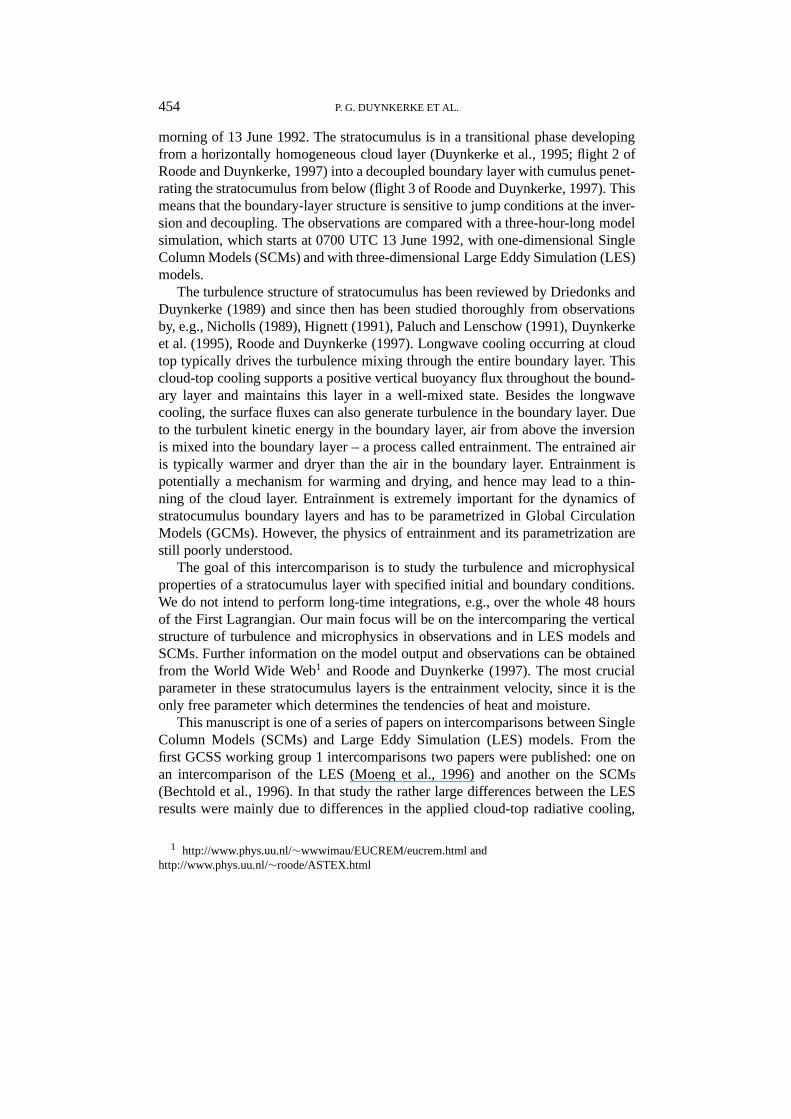
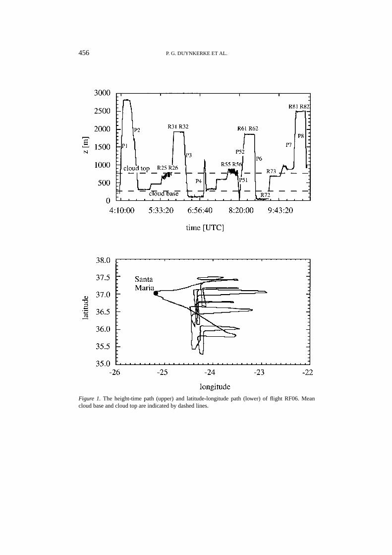
Detailed information about the boundary-layer structure is based on aircraft ob-servations made east of Santa Maria (Figure 1) between 0407 UTC and 1042 UTCon 13 June 1992. In Duynkerke et al. (1995) the synoptic situation is discussed onthe basis of the initialized analysis of the ECMWF model for 13 June 0000 UTC.At that time a surface high pressure system was situated near 36◦ N, 28◦ W (theirFigure 3a). The experimental area (Figure 1b) is thus slightly east of the centre ofthe high pressure system. The NOAA AVHRR satellite picture in Figure 2 clearlyshows the low level cloud over the experimental area. From the ECMWF analysison 13 June (Duynkerke et al., 1995) it is clear that the air in the experimentalarea has moved southwards and that in this direction the sea surface temperature isincreasing (Roode and Duynkerke, 1997).

The latitude-longitude co-ordinates of the flight track are shown in Figure 1b.Flights were made at different levels above, within and below cloud, as shown inFigure 1a. Three stacks and numerous profiles were obtained. The navigation wassuch that the aircraft remained roughly in the same air mass. At a certain heighthorizontal runs of about 10 minutes duration were flown in ‘L’ shaped legs. These‘L’ shaped legs consisted of an initial crosswind leg (wind in the boundary layeris from about 10◦) followed by a southward turn to a downwind leg, each lasting

456 P. G. DUYNKERKE ET AL.

Figure 1. The height-time path (upper) and latitude-longitude path (lower) of flight RF06. Meancloud base and cloud top are indicated by dashed lines.

INTERCOMPARISON OF THREE- AND ONE-DIMENSIONAL MODEL SIMULATIONS 457

Figure 2. NOAA AVHRR channel 1 satellite picture for 0925 UTC 13 June 1992 at about 24◦ W(vertical line) and 37◦ N. The size of the domain is about 240× 240 km2. Convective cloud structurescan be seen in the stratocumulus deck with a horizontal size ranging from one tenth to several tenthsof a kilometer.

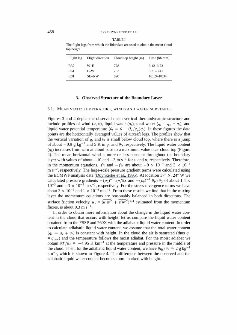
about 10 minutes. With a flight speed of about 100 m s−1, a 10 min flight covereda distance of about 60 km. Horizontal runs were flown between 30 m to 2800 mabove the sea surface. Four porpoise runs were flown from about 100 m aboveto about 100 m below cloud top; they are numbered R25, R26, R55 and R56. Inaddition, ‘profiles’ were flown; these profiles are numbered P1, P2, P3, P4, P51,P52, P6, P7 and P8. The cloud top height was determined from the FSSP liquidwater content measured during the porpoise runs (R25, R26, R55 and R56) as wellas from lidar information (Table I). Within the experimental area the lowest cloudbase was at about 280 m and cloud top was at about 770 m. There were smallcumulus clouds under the stratocumulus deck.

458 P. G. DUYNKERKE ET AL.

TABLE I

The flight legs from which the lidar data are used to obtain the mean cloudtop height.

Flight leg Flight direction Cloud top height (m) Time (hh:mm)

R32 W–E 728 6:12–6:23

R61 E–W 762 8:31–8:41

R81 SE–NW 820 10:19–10:34

3. Observed Structure of the Boundary Layer

3.1. MEAN STATE: TEMPERATURE, WINDS AND WATER SUBSTANCE

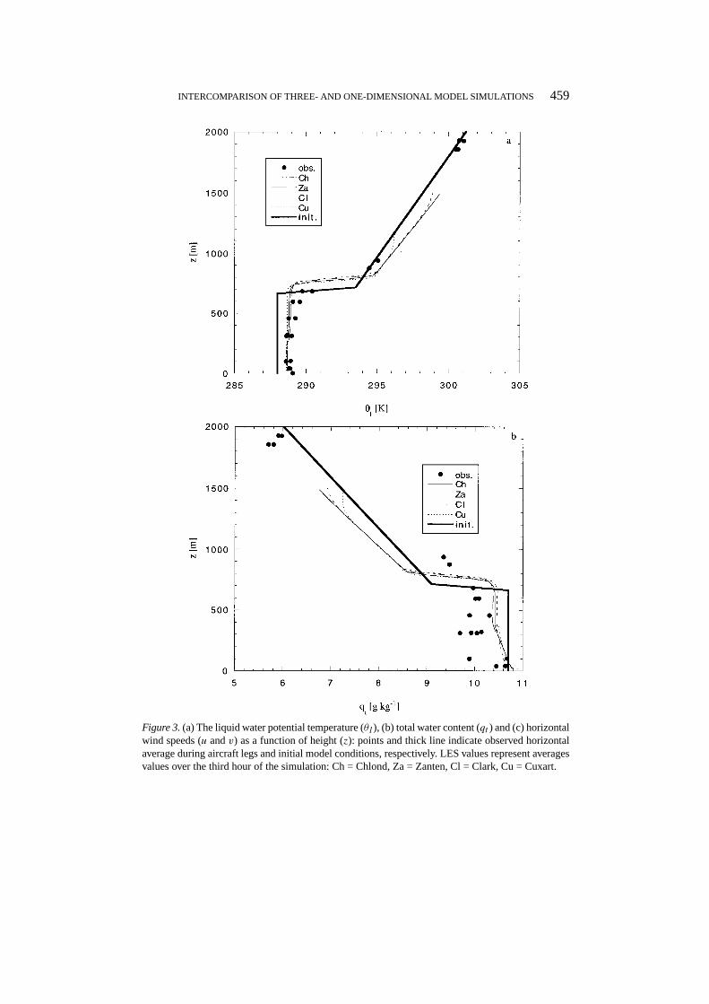
Figures 3 and 4 depict the observed mean vertical thermodynamic structure andinclude profiles of wind(u, v), liquid water (ql), total water (qt = qv + ql), andliquid water potential temperature (θl = θ − (lv/cp)ql). In these figures the datapoints are the horizontally averaged values of aircraft legs. The profiles show thatthe vertical variation ofqt andθl is small below cloud top, where there is a jumpof about−0.9 g kg−1 and 5 K inqt andθl, respectively. The liquid water content(ql) increases from zero at cloud base to a maximum value near cloud top (Figure4). The mean horizontal wind is more or less constant throughout the boundarylayer with values of about−10 and−3 m s−1 for v andu, respectively. Therefore,in the momentum equations,f v and−f u are about−9 × 10−4 and 3× 10−4

m s−2, respectively. The large-scale pressure gradient terms were calculated usingthe ECMWF analysis data (Duynkerke et al., 1995). At location 37◦ N, 24◦ W wecalculated pressure gradients−(ρ0)−1 ∂p/∂x and−(ρ0)

−1 ∂p/∂y of about 1.4×10−3 and−3× 10−4 m s−2, respectively. For the stress divergence terms we haveabout 3× 10−5 and 1× 10−4 m s−2. From these results we find that in the mixinglayer the momentum equations are reasonably balanced in both directions. The

surface friction velocity,u∗ = (u′w′2 + v′w′2)1/4 estimated from the momentumfluxes, is about 0.3 m s−1.

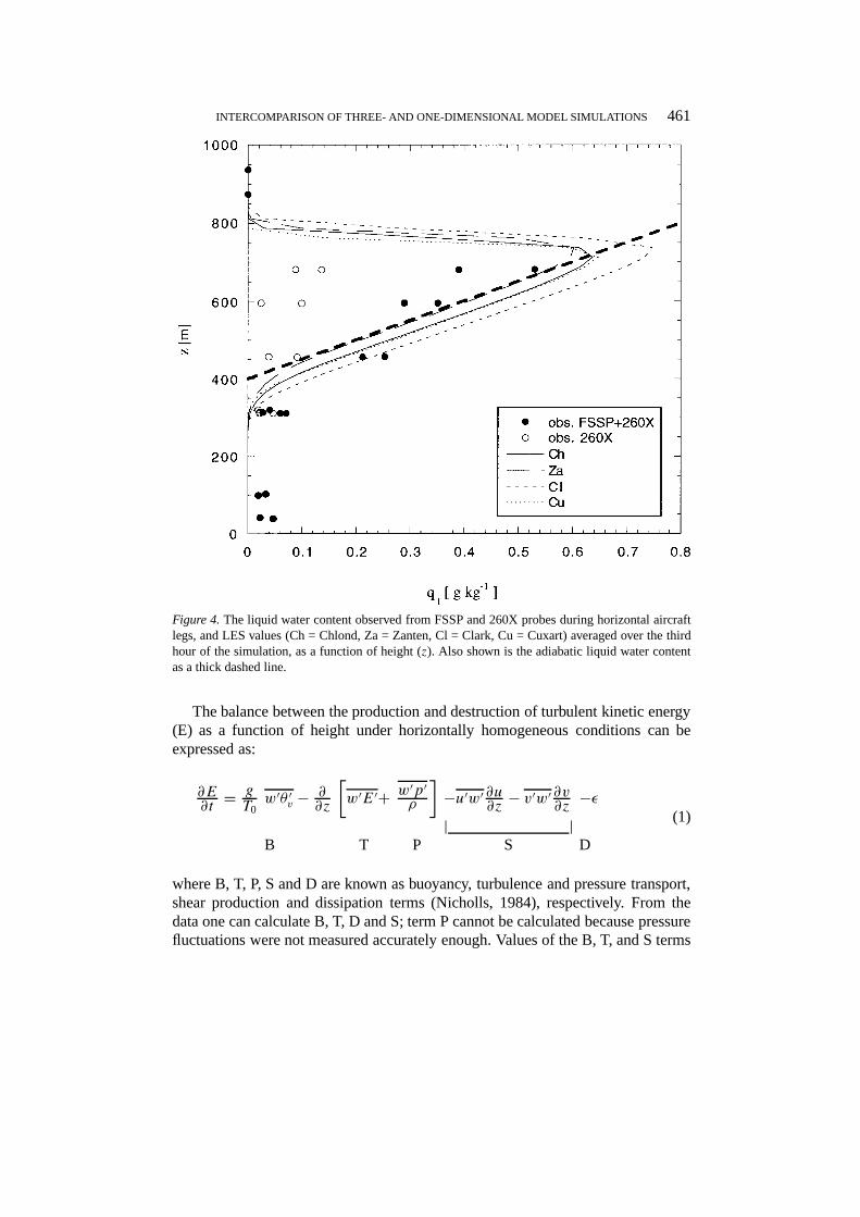
In order to obtain more information about the change in the liquid water con-tent in the cloud that occurs with height, let us compare the liquid water contentobtained from the FSSP and 260X with the adiabatic liquid water content. In orderto calculate adiabatic liquid water content, we assume that the total water content(qt = qv + ql) is constant with height. In the cloud the air is saturated (thusqv= qvsat) and the temperature follows the moist adiabat. For the moist adiabat weobtain∂T /∂z ≈ −4.95 K km−1 at the temperature and pressure in the middle ofthe cloud. Then, for the adiabatic liquid water content, we have∂ql/∂z ≈ 2 g kg−1

km−1, which is shown in Figure 4. The difference between the observed and theadiabatic liquid water content becomes more marked with height.

INTERCOMPARISON OF THREE- AND ONE-DIMENSIONAL MODEL SIMULATIONS 459

Figure 3.(a) The liquid water potential temperature (θl), (b) total water content (qt ) and (c) horizontalwind speeds (u andv) as a function of height (z): points and thick line indicate observed horizontalaverage during aircraft legs and initial model conditions, respectively. LES values represent averagesvalues over the third hour of the simulation: Ch = Chlond, Za = Zanten, Cl = Clark, Cu = Cuxart.

460 P. G. DUYNKERKE ET AL.

Figure 3.Continued.

3.2. STRUCTURE OF TURBULENCE

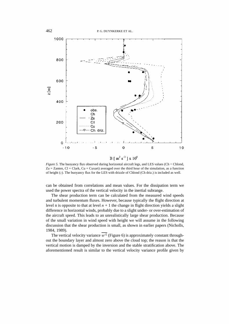
The virtual potential temperature flux is used to express the buoyancy flux. Thevalue of the virtual potential temperature flux depends on moisture flux (wqv), li-quid water content flux (wql) and potential temperature flux (wθ) (Stull, 1988). Thebuoyancy fluxes measured during flight RF06 are shown in Figure 5. Maximumbuoyancy flux values are observed in the cloud layer and at the ocean surface. Thisimplies that both cloud top radiative cooling and surface convection are importantbuoyancy production mechanisms. Entrainment takes the potentially warmer airfrom above the inversion down into the cloud; this leads to a minimum in thebuoyancy flux at cloud top (actually the buoyancy flux should become negative butthis occurs only over a small height interval which measurements cannot resolve).From the surface upwards the buoyancy flux decreases to small or even negativevalues near cloud base. For the cloud-topped boundary layer a general convectivescaling is not available because the buoyancy flux is not a simple universal functionof height as in the clear convective boundary layer (CBL). Therefore the results thatare presented will not be normalized as is typically done in the CBL.

INTERCOMPARISON OF THREE- AND ONE-DIMENSIONAL MODEL SIMULATIONS 461

Figure 4.The liquid water content observed from FSSP and260X probes during horizontal aircraftlegs, and LES values (Ch = Chlond, Za = Zanten, Cl = Clark, Cu = Cuxart) averaged over the thirdhour of the simulation, as a function of height (z). Also shown is the adiabatic liquid water contentas a thick dashed line.

The balance between the production and destruction of turbulent kinetic energy(E) as a function of height under horizontally homogeneous conditions can beexpressed as:

∂E∂t= gT0

w′θ ′v − ∂∂z

[w′E′+ w′p′

ρ

]−u′w′ ∂u

∂z− v′w′ ∂v

∂z−ε

| |B T P S D

(1)

where B, T, P, S and D are known as buoyancy, turbulence and pressure transport,shear production and dissipation terms (Nicholls, 1984), respectively. From thedata one can calculate B, T, D and S; term P cannot be calculated because pressurefluctuations were not measured accurately enough. Values of the B, T, and S terms

462 P. G. DUYNKERKE ET AL.

Figure 5.The buoyancy flux observed during horizontal aircraft legs, and LES values (Ch = Chlond,Za = Zanten, Cl = Clark, Cu = Cuxart) averaged over the third hour of the simulation, as a functionof height (z). The buoyancy flux for the LES with drizzle of Chlond (Ch driz.) is included as well.

can be obtained from correlations and mean values. For the dissipation term weused the power spectra of the vertical velocity in the inertial subrange.

The shear production term can be calculated from the measured wind speedsand turbulent momentum fluxes. However, because typically the flight direction atlevel n is opposite to that at leveln + 1 the change in flight direction yields a slightdifference in horizontal winds, probably due to a slight under- or over-estimation ofthe aircraft speed. This leads to an unrealistically large shear production. Becauseof the small variation in wind speed with height we will assume in the followingdiscussion that the shear production is small, as shown in earlier papers (Nicholls,1984, 1989).

The vertical velocity variancew′2 (Figure 6) is approximately constant through-out the boundary layer and almost zero above the cloud top; the reason is that thevertical motion is damped by the inversion and the stable stratification above. Theaforementioned result is similar to the vertical velocity variance profile given by

INTERCOMPARISON OF THREE- AND ONE-DIMENSIONAL MODEL SIMULATIONS 463

Figure 6.The vertical velocity variance observed during horizontal aircraft legs, and LES values (Ch= Chlond, Za = Zanten, Cl = Clark, Cu = Cuxart) averaged over the third hour of the simulation, asa function of height (z). The vertical velocity variance for the LES with drizzle of Chlond (Ch driz.)is included as well.

Nicholls (1989). In our case the surface buoyancy flux (Figure 5) is as large as, oreven slightly larger than the in-cloud buoyancy flux. This means that the surfacebuoyancy flux and in-cloud buoyancy flux are both equally important in driving theconvection (turbulence).

On board the Electra a lidar was flown that could be used to measure the cloudtop height. The minimum distance between the cloud and the aircraft had to be700 m. Therefore only the data from the runs high enough above the cloud (R32,R31, R61, R62, R81 and R82) can be used (Table I). The most reliable data areobtained from the nearly cross-wind flights (R32, R61 and R81) because of thenorth-south sea surface temperature gradient. From these we obtain an averageboundary-layer growth rate∂h/∂t = 0.62× 10−2 m s−1. The subsidence velocitywas estimated from the initialized analysis of the ECMWF model and the ASTEXradiosondes, giving a value of aboutws = 0.38× 10−2 m s−1. From these results

464 P. G. DUYNKERKE ET AL.

we can estimate the entrainment velocity:we = ∂h/∂t + ws = 1.0 (± 0.6)× 10−2

m s−1. This is in good agreement with the entrainment velocity of 1.2 (± 1.0)×10−2 m s−1 estimated from ozone fluxes near the inversion (Roode and Duynkerke,1997). In the future it will be necessary to make better observations of subsidencein order to estimate the entrainment velocity more accurately.

In DeLaat and Duynkerke (1998) the mass-flux approach is applied to the dataobtained during three flights of the NCAR Electra during the first Lagrangian ofASTEX. Here we will use their results for flight RF06. In a mass-flux approachthe boundary layer is divided into ‘updrafts’ and ‘downdrafts’. This can be donein several ways: e.g., by the sign of the vertical velocity, by a vertical velocitythreshold (with a combination of a threshold for the updraft and downdraft size)or by using moisture (see Randall et al., 1992 for a summary). In DeLaat andDuynkerke (1998) the sign of the vertical velocity was chosen as the definition forupdrafts and downdrafts. This means that the small-scale turbulence (down to 5 m)is also included in the data analysis.

In a mass-flux approach the average values of quantities like temperature andmoisture are calculated for both updrafts and downdrafts. The average values forthe entire layer are written as (Randall et al., 1992):

ψ = σψu + (1− σ )ψd (2)

in whichψu,d are the average values of a quantityψ for the updraft and downdraftrespectively andσ is the updraft fractional area. The fluxes of a quantityψ can bewritten as (Randall et al., 1992):

Fψm = Mc(ψu − ψd) ≈ C(ρ0w′ψ ′) (3)

with ρ0 the air density,C the ratio of the flux from the mass-flux approach and thereal (measured) flux,Fψm the flux of the scalarψ in the mass-flux approach, andMc the mass flux defined as:

Mc ≡ ρ0σ (wu − w) = ρ0σ (1− σ )(wu − wd). (4)

Equation (3) is an important result of this approach; the fluxes of a certain scalarare proportional to the difference between the average values of the scalar for theupdraft and the downdraft. The observed values for the updraft fractional area andmass flux are shown in Figures 7 and 8, respectively. The updraft fractional areaof about 50% indicates a nearly symmetric probability density function for thevertical velocity.

3.3. CLOUD MICROPHYSICS

The concentration of droplets (N) can be calculated fromN = ∫ r2r1n(r) dr, in

which n(r) is the number density of drops, andr1 andr2 are the upper and lower

INTERCOMPARISON OF THREE- AND ONE-DIMENSIONAL MODEL SIMULATIONS 465

Figure 7.The updraft fractional area observed during horizontal aircraft legs, and LES values (Ch =Chlond, Za = Zanten, Cl = Clark, Cu = Cuxart) averaged over the third hour of the simulation, as afunction of height (z).

boundaries of the radius interval over which the droplets are measured (3≤ d ≤66µm for the FSSP data and for 260X we used 65≤ d ≤ 625µm in order to haveno overlap with FSSP interval). The last interval of the FSSP and the first intervalof the 260X are centred at 64.25 and 70µm, respectively. From the observations(Figure 9a) we find that inside the cloud the total concentration of drops (N) isreasonably constant with height. The increase ofql with height (Figure 4) is thusaccounted for by an increase in the mean volume of the drops rather than by anincrease in concentration. The drop contribution (about 120 cm−3) is determinedalmost entirely by the smaller size drops (FSSP) and there are only about 50 largesize (65≤ d ≤ 625µm) drops per dm3 (Figure 9a). About 20% of the liquid watercontent in the cloud layer is due to the larger droplets (260X probe) as shown inFigure 4. Below cloud base almost all liquid water is due to the larger droplets.

466 P. G. DUYNKERKE ET AL.

Figure 8.The mass flux observed during horizontal aircraft legs, and LES values (Ch = Chlond, Za= Zanten, Cl = Clark, Cu = Cuxart) averaged over the third hour of the simulation, as a function ofheight (z).

In order to evaluate the rainfall rate term (̃wT ql) we calculated mean drop sizespectra for each horizontal run and evaluated the rainfall rate from:

w̃T ql = ρw

ρ0

∫ ∞0

4π

3wT (r)n(r)r

3dr (5)

where the droplet terminal velocitywT is given by (Rogers, 1979):

wT (r) ={

1.19× 108r2 m s−1 for r < 40× 10−6 m8× 103rm s−1 for r ≥ 40× 10−6 m

(6)

whereρw is the density of liquid water (1000 kg m−3), ρ0 is the air density,n(r) isthe number density of drops andr is the radius.

In Figure 9b the number density concentration∫1rn(r) dr (1r = 4µm for FSSP

and1r = 20µm for 260X) is shown for run R73 in the cloud and run R72 belowcloud base (Figure 1). From this figure we can see that in the cloud the number

INTERCOMPARISON OF THREE- AND ONE-DIMENSIONAL MODEL SIMULATIONS 467

Figure 9.(a) Variation in droplet concentration with height for small (FSSP probe) and large (260Xprobe) droplets. (b) Mean droplet spectra at two heights from FSSP and260X probes obtained duringruns R72 (41 m) and R73 (681 m). The last interval of the FSSP and the first interval of the260Xare centred at 64.25 and 70µm, respectively. Also plotted are isolines of liquid water content in gkg−1 per interval (dashed lines) and rainfall rate in m s−1 per interval (thin full lines). Note that theisolines of rainfall rate have a kink at a diameter of 80µm according to (6).

468 P. G. DUYNKERKE ET AL.

density concentration is at its maximum at a radius of about 10µm. The dip in thedroplet spectra at about 30µm radius is due to the measurement error of the FSSPand 260X probes in their upper and lower size range, respectively.

Figure 9b also shows the relative contribution made by each radius interval tothe total liquid water content and the rainfall rate. In this figure the isolines of liquidwater content (ql) are proportional tor−3, and the isolines of rainfall rate (̃wT ql)are proportional tor−5 andr−6 for droplet radii, which are smaller and larger than40µm, respectively (see Equation (6)). This figure shows that droplets smaller thanabout 15µm contribute most to the liquid water content. The rainfall rate in thewhole boundary layer (Figure 12 to be discussed later) is mainly due to the largerdrops.

4. Model Simulations

The primary objective of EUCREM is to develop parametrization schemes forcloud processes within the GCMs being used. The improvement of the paramet-rization schemes will be quantified by comparing single-column models againstcloud-resolving models. The goal is to study the turbulence and microphysicalproperties of a stratocumulus layer given the initial and boundary conditions. Twosimulations are performed, one in which the terminal fall-velocity of droplets is setto zero and another simulation including drizzle. Both LES and the SCM had touse the same initial conditions and vertical resolution (25 m). The 25-m verticalresolution in the SCM was used to minimise numerical errors in the simulations.The SCM versions of the ECMWF and Hadley Centre GCM were run only withthe operational vertical resolutions (ECMWF had levels at about 30, 150, 360,640 and 990 m) because the physical parametrizations had been tuned to theseresolutions. A summary of the LES and SCM results is given in Sections 4.2 and4.3, respectively. The complete data set can be found on the World Wide Web (seeearlier footnote).

4.1. MODEL INITIALIZATION AND FORCING

The initial and boundary conditions are based on the observations described in thepreceding sections. The geostrophic wind is set to (ug, vg) = (−3, −10) m s−1.Initial profiles for horizontal wind components, liquid water potential temperature(θl) and total water content (qt ) are:

INTERCOMPARISON OF THREE- AND ONE-DIMENSIONAL MODEL SIMULATIONS 469

0< z ≤ 662.5 m (u, v) = (−1.7,−10.0) (m s−1)

θl = 288.0 (K)

qt = 10.7 (g kg−1)

662.5 < z ≤ 712.5 m u = −1.7− 0.026(z − 662.5) (m s−1)

v = −10.0 (m s−1)

θl = 288.0+ 0.11(z − 662.5) (K)

qt = 10.7− 0.032(z − 662.5) (g kg−1)

712.5 < z < 1500 m (u, v) = (−3,−10) (m s−1)

θl = 293.5+ 6× 10−3(z − 712.5) (K)

qt = 9.1− 2.4× 10−3(z− 712.5) (g kg−1).

(7)

The profiles between the base (662.5 m) and the top of the inversion (712.5 m)are linear interpolations between the boundary-layer values and free troposphericvalues at 712.5 m. The jumps at the inversion are thus1θl = 5.5 K and1qt =− 1.6g kg−1 (1θe = 1.5 K). The initial profiles forθl, qt , u andv are shown in Figure 3together with the observations. The initial total water content in the boundary layerhas been increased compared to the observations in order to obtain the correctheight of the cloud base.

The surface fluxes are prescribed as:

uw = − u

(u2+ v2)1/2u2∗

vw = − v

(u2+ v2)1/2u2∗ (8)

wθ = wθ1 = 0.013 K m s−1

wqt = 1.8× 10−5 m s−1 kg kg−1

whereu∗ = 0.3 m s−1 and the velocities (u andv) are the values at the lowest gridpoint level in the model. In the formulation above, the surface fluxes at each gridpoint are the same.

The net longwave radiation is parametrized as

FL(z) = 1Ft exp[−aLWP(z, zt)], (9)

where1Ft = 74 W m−2 is the longwave cooling at cloud top,a = 130 m2 kg−1

a constant andzt (=1500 m) is the top of the model domain. LWP(z1, z2) is theliquid water path betweenz1 andz2 and is defined as:

LWP(z1, z2) =∫ z2

z1

ρ0ql dz with ρ0 = 1.1436 kg m−3. (10)

The net shortwave radiation is kept at zero.

470 P. G. DUYNKERKE ET AL.

The divergence is set at 1.5× 10−5 s−1 and therefore the mean vertical velocityis prescribed as:ws = −1.5×10−5 z. The subsidence is taken into account througha large-scale forcing term (source term) in the governing equations (Sommeria,1976). The initialized analysis of the ECMWF and radiosondes give a divergenceof about 5× 10−6 s−1, but in the 1996 intercomparison of working group 1 of theGCSS1 it was found that the divergence must have been about 1.5× 10−5 s−1 inorder to get a boundary-layer depth close to the observed value (Duynkerke et al.,2000). The vertical velocities of the ECMWF model are extremely noisy even inthese high pressure regions, both in space and time. This means that the subsidencevelocity is not very reliable, especially over data-sparse regions such as the oceans.However, on a time scale of three hours the subsidence velocity is not importantfor the turbulence; it only determines the depth of the boundary layer. Thus for theintercomparison of the turbulence and microphysics the value of the subsidence isnot very important. If the subsidence is lowered the cloud top will rise more rapidlyand the intercomparison with observations will be more complicated because themodelled cloud will be shifted in the vertical compared to the observations.

The Coriolis parameter is set tof = 8.7× 10−5 s−1 (latitude of about 36.6◦N); the surface pressure is 1028.8 hPa. For the LES model periodic boundaryconditions were applied. A spatially uncorrelated random perturbation, uniformlydistributed between−0.1 and 0.1 K, was applied to the initial temperature field atall grid points withz < 687.5 m. An initial value for subgrid TKE of 1 m2 s−2 wasspecified forz < 687.5 m. The inversion heightzi is determined byqt = 9.4 g kg−1,obtained by linear interpolation between adjacent grid levels of total water content.The grid size is 50 m in the horizontal directions (x andy) and 25 m in the vertical(z), covering a domain of 3.2 km inx andy and 1.5 km inz.

4.2. LESRESULTS

Four LES models were used for the intercomparison. The results are summarizedin Tables II and III. Addresses of the participants and references to the model de-scriptions are given in Appendix A. All four LES models have different roots and assuch have very different numerical schemes. Three of the LES models have a TKEequation as a subgrid scale model and one model uses a Smagorinsky (1963)–Lilly(1967) (SL) closure. In the SL model it is assumed that the shear and buoyancyproduction in the subgrid TKE balance are locally balanced by dissipation. Theresulting eddy viscosity depends on the local shear and temperature gradients. Forthe subgrid condensation scheme three models use an ‘all-or-nothing’ (AN) schemeand one model uses a scheme developed by Sommeria and Deardorff (1977) (SD).The AN scheme assumes that within each grid box the air is either entirely unsat-urated or saturated. The SD scheme allows for partial cloudiness, depending on theSGS variances of the thermodynamic variables.

1 http://www.phys.uu.nl/∼wwwimau/ASTEX/astexcomp.html

INTERCOMPARISON OF THREE- AND ONE-DIMENSIONAL MODEL SIMULATIONS 471

TABLE II

The scientists, model groups, model dimension (d), subgrid scale (SGS)turbulence and condensation schemes. The abbreviations of the modelgroups are explained in Appendix A. TKE: turbulent kinetic energy, S-L:Smagorinsky-Lilly, AN: “all-or-nothing”, SD: Sommeria and Deardorff(1977).

Scientist Model group d SGS turbulence SGS condensation

Chlond MPI 3 TKE SD

Zanten IMAU 3 TKE AN

Clark UMIST 3 S-L AN

Cuxart/S. INM 3 TKE AN

Cuxart/S. INM 1 1.5 order AN/SD

Lenderink KNMI 1 1.5 order RH

Martin Hadley C. 1 Smith (1994) Smith (1990)

Teixeira ECMWF 1 K-closure Tiedtke (1993)

TABLE III

The average properties during the third hour of the simulation: entrainment velocity (we),convective velocity scale (w∗), Richardson number (Riw∗) and at the third hour: inversionheight (zi ) and liquid water path (LWP). Simulations on the same domain but with a highvertical (10 m) resolution (h.v.r.) and a higher resolution (25× 25× 10 m3) in all directions(h.r.) are included as well. Two SCMs were run at the operational vertical resolution whichis a coarser vertical resolution (c.v.r.) than prescribed.

we w∗ Riw∗ (we/w∗) A zi (m) LWP

(cm s−1) (m s−1) × 100 (g m−2)

Chlond 1.95 0.790 184 2.47 4.54 776 159

Zanten 2.02 0.697 238 2.89 6.88 803 139

Zanten h.v.r. 1.95 0.742 205 2.63 5.41 794 160

Zanten h.r. 2.02 0.831 158 2.43 3.84 785 171

Clark 1.95 0.882 139 2.21 3.08 805 180

Cuxart/S. 1.79 0.808 216 2.22 4.80 779 158

Cuxart/S. 1.08 0.975 137 1.11 1.51 720 191

Lenderink 1.72 0.637 271 2.70 7.31 765 198

Martin c.v.r. – – – – – 697 214

Teixeira c.v.r. – – – – – 772 233

472 P. G. DUYNKERKE ET AL.

The vertical profile of the liquid water content, averaged over the third hour ofthe simulation, is shown in Figure 4. For comparison the adiabatic liquid watercontent is shown as well. It is clear that the LES models all predict an adiabaticliquid water content in the bulk of the boundary layer. The observations indicate anLWC lower than the adiabatic values. This might be due to instrumental problems(Bower and Choularton, 1992; Gerber, 1996) that systematically tend to underes-timate the LWC, or to the presence of drizzle when the observations were beingmade. The latter will reduce the LWC below its adiabatic value, a topic that will bediscussed briefly below.

The turbulence simulated within the stratocumulus-topped boundary layer isdriven both by longwave radiative cooling at cloud top and a surface buoyancyflux. The jump in the net longwave flux at cloud top is 74 W m−2 for all models,as prescribed. Due to the coarse vertical resolution (25 m), typically 40% of the 74W m−2 cooling takes place over one grid point. This means that the buoyancy fluxis not very well resolved near cloud top (Figure 5).

Vertical profiles of the total (resolved plus subgrid) buoyancy flux, averagedover the third hour of the simulation, are shown in Figure 5. Three of the LESmodels (Ch, Za and Cu) yield very similar buoyancy profiles that are in reasonableagreement with the observations. These LES models all show a slightly negativebuoyancy flux near cloud base, indicating a tendency towards a fairly stable strat-ification near cloud base (tendency towards decoupling). One of the LES models(Cl) gives a somewhat larger buoyancy flux throughout the boundary layer. Thusthe LES models over-predict the buoyancy production compared with the obser-vations. The fairly stable layer near cloud base creates a small local minimum inthe vertical velocity variance (Figure 6) near cloud base. These three LES modelsgive vertical velocity variance profiles that are in reasonable agreement with theobservations. The LES model Cl gives vertical velocity variances that are too largecompared with the observations.

For the cloud-topped boundary layer a generalized convective velocity scaleis typically used which, instead of depending only on the surface buoyancy flux,depends on the buoyancy flux integrated over the whole boundary-layer depth:

w3∗ = 2.5

∫ h

0(g/θ0)w′θ ′vdz. (11)

The constant 2.5 is fixed by the fact that for the dry convective boundary layer(CBL) Equation (11) reduces to its basic definition in the CBL, given a typicalentrainment flux at the boundary-layer height (h) (w′θ ′v)h = −A(w′θ ′v)s , with A =0.2. Sometimes is assumed that the entrainment velocity scales withw∗ andh as(Deardorff, 1976):

we/w∗ = ARi−1w∗ with Riw∗ = (g/θ0)1θvh

w2∗(12)

INTERCOMPARISON OF THREE- AND ONE-DIMENSIONAL MODEL SIMULATIONS 473

where1θv stands for the virtual potential temperature jump over the inversion.The values for A obtained from the LES simulations are given in Table III. It isclear that a typical value for A in stratocumulus is at least one order of magnitudelarger than a typical value of A for the CBL. Therefore the scaling relationship(11) does not hold for a stratocumulus-topped boundary layer. The different scalinglaws of the entrainment velocity have been discussed recently in papers by Lockand MacVean (1999) and vanZanten et al. (1999). In vanZanten et al. (1999) threeclosures for the entrainment flux are evaluated for different types of convectiveboundary layer; CBL, smoke and stratocumulus. The general conclusion is thatthe convective scaling (11) is not a very good parametrization and that processpartitioning (Stage and Businger, 1981) is much superior.

In this paper we will discuss only two quantities for the mass-flux approach (lastpart of Section 3): the updraft fractional area (σ ) and the mass-flux (Mc). Both ob-servations and LES results yield an updraft fractional area close to 0.5 throughoutthe boundary layer (Figure 7). This means that the vertical velocity distributionis hardly skewed (DeLaat and Duynkerke, 1998). The simulated mass flux is inreasonable agreement with the observations (Figure 8) made at various levels in theboundary layer. It is important to note that the mass flux in stratocumulus-toppedboundary layers (about 0.2 kg m−2 s−1) is an order of magnitude larger than fordeep convection (about 0.01 kg m−2 s−1). For all LES models the ratio of the fluxin the mass-flux approach and the total flux (3) is about 0.6, as was found from theobservations.

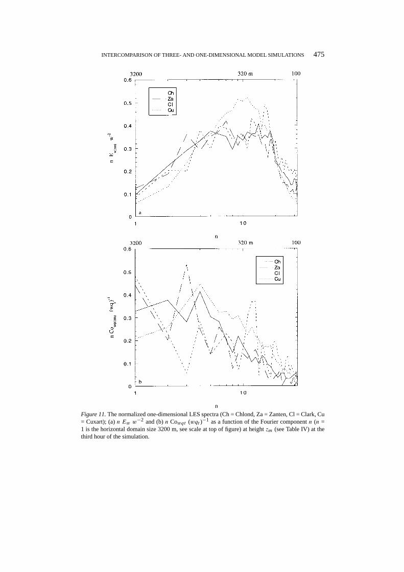
In Figures 10 and 11 the (co)spectra of the vertical velocity and total water fluxat a height of 600 m andzm are plotted. The heightzm is defined as the heightwhere the buoyancy flux at the inversion attains its minimum value (see Table IV).The vertical velocity spectra in the middle of the cloud layer indicate that the mostenergetic eddies have a the same horizontal scale as the depth of the boundary layer.The corresponding cospectra of the total water flux show that most of the flux istransported by eddies which are the size of the horizontal domain. This is the resultof mesoscale structures which develop in these stratocumulus-topped boundarylayers, a topic which is discussed in detail by Jonker et al. (1999). The mesocalestructures contain energy at the large scales (larger than the boundary-layer depth)and are present in the energy spectra of all variables (u, v, θl, qt , ql , etc.), except forthe vertical velocity (w). These mesoscale structures are easily generated in LES(Jonker et al., 1999) and the largest size of these mesoscale structures typicallyincreases with time. For the chosen domain (3.2× 3.2 km2) the largest scales at 3h are about the size of the domain. We performed simulations on a 6.4× 6.4 km2

and 12.8× 12.8 km2 horizontal domain and found that the results are quite robust;changes in fluxes and variance are less than 10% and 20% respectively.

The (co)spectra at the inversion are given in Figure 11. Figure 11a shows thateddies contributing most to the vertical velocity variance at the inversion have ahorizontal size of about half the boundary-layer depth (about 300 m). The cospectraof the total water flux (Figure 11b) indicate that even at the inversion the vertical

474 P. G. DUYNKERKE ET AL.

Figure 10.The normalized one-dimensional LES spectra (Ch = Chlond, Za = Zanten , Cl = Clark,Cu = Cuxart); (a)n Ew w−2 and (b)n Cowqt (wqt )−1 as a function of the Fourier componentn (n= 1 is the horizontal domain size 3200 m, see scale at top of figure) at a height of 600 m at the thirdhour of the simulation.

INTERCOMPARISON OF THREE- AND ONE-DIMENSIONAL MODEL SIMULATIONS 475

Figure 11.The normalized one-dimensional LES spectra (Ch = Chlond, Za = Zanten, Cl = Clark, Cu= Cuxart); (a)n Ew w−2 and (b)n Cowqt (wqt )−1 as a function of the Fourier componentn (n =1 is the horizontal domain size 3200 m, see scale at top of figure) at heightzm (see Table IV) at thethird hour of the simulation.

476 P. G. DUYNKERKE ET AL.

TABLE IV

The correlation coefficient (r) between vertical velocity (w) and total water content(qt ) at a height of 100 m, 600 m andzm (the height where the buoyancy flux attainsa minimum value at the inversion) calculated from the 1-dimensional spectral data ofthe resolved LES fields.

r(wqt ) r(wqt ) r(wqt ) zm w2 (zm) q2t (zm) wqt (zm)

100 m 600 m zm m × 108 × 104

Chlond 0.59 0.62 0.30 775 0.045 10.4 0.20

Zanten 0.47 0.66 0.41 800 0.084 6.92 0.32

Clark 0.56 0.50 0.15 813 0.020 14.5 0.08

Cuxart 0.59 0.55 0.34 800 0.016 5.57 0.10

flux is transported mainly by eddies which have a horizontal scale of roughly thedepth of the boundary layer. Further research is needed in order to explain whichscale of the eddies is responsible for most of the entrainment.

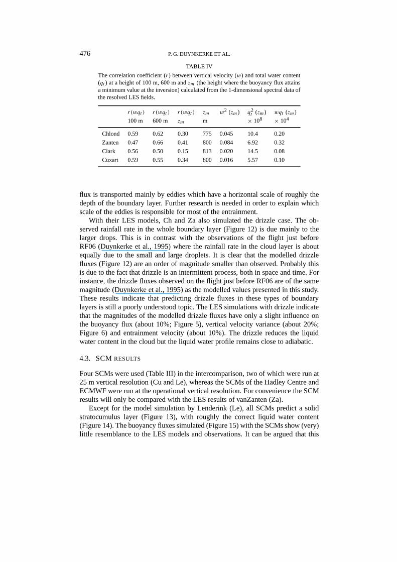
With their LES models, Ch and Za also simulated the drizzle case. The ob-served rainfall rate in the whole boundary layer (Figure 12) is due mainly to thelarger drops. This is in contrast with the observations of the flight just beforeRF06 (Duynkerke et al., 1995) where the rainfall rate in the cloud layer is aboutequally due to the small and large droplets. It is clear that the modelled drizzlefluxes (Figure 12) are an order of magnitude smaller than observed. Probably thisis due to the fact that drizzle is an intermittent process, both in space and time. Forinstance, the drizzle fluxes observed on the flight just before RF06 are of the samemagnitude (Duynkerke et al., 1995) as the modelled values presented in this study.These results indicate that predicting drizzle fluxes in these types of boundarylayers is still a poorly understood topic. The LES simulations with drizzle indicatethat the magnitudes of the modelled drizzle fluxes have only a slight influence onthe buoyancy flux (about 10%; Figure 5), vertical velocity variance (about 20%;Figure 6) and entrainment velocity (about 10%). The drizzle reduces the liquidwater content in the cloud but the liquid water profile remains close to adiabatic.

4.3. SCMRESULTS

Four SCMs were used (Table III) in the intercomparison, two of which were run at25 m vertical resolution (Cu and Le), whereas the SCMs of the Hadley Centre andECMWF were run at the operational vertical resolution. For convenience the SCMresults will only be compared with the LES results of vanZanten (Za).

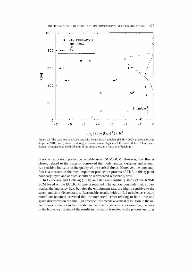
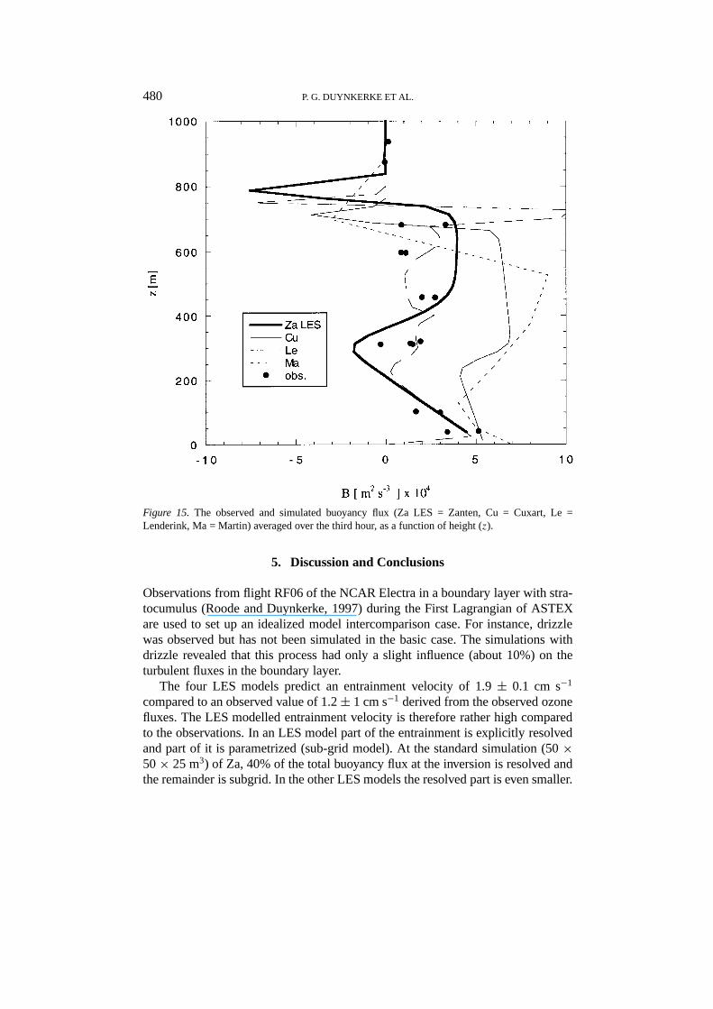
Except for the model simulation by Lenderink (Le), all SCMs predict a solidstratocumulus layer (Figure 13), with roughly the correct liquid water content(Figure 14). The buoyancy fluxes simulated (Figure 15) with the SCMs show (very)little resemblance to the LES models and observations. It can be argued that this

INTERCOMPARISON OF THREE- AND ONE-DIMENSIONAL MODEL SIMULATIONS 477

Figure 12.The variation of drizzle rate with height for all droplets (FSSP +260X probe) and largedroplets (260X probe) observed during horizontal aircraft legs, and LES values (Ch = Chlond, Za =Zanten) averaged over the third hour of the simulation, as a function of height (z).

is not an important predictive variable in an SCM/GCM. However, this flux isclosely related to the fluxes of conserved thermodynamical variables and as suchis a sensitive indicator of the quality of the vertical fluxes. Moreover, the buoyancyflux is a measure of the most important production process of TKE in this type ofboundary layer, and as such should be represented reasonably well.

In Lenderink and Holtslag (1998) an extensive sensitivity study of the KNMISCM based on the EUCREM case is reported. The authors conclude that, in par-ticular, the buoyancy flux, but also the entrainment rate, are highly sensitive to thespace and time discretization. Reasonable results with an E-l turbulence closuremodel are obtained provided that the numerical errors relating to both time andspace discretization are small. In practice, this means a vertical resolution in the or-der of tens of metres and a time step in the order of seconds. (For example, the peakin the buoyancy forcing of the results in this study is related to the process-splitting

478 P. G. DUYNKERKE ET AL.

Figure 13. The observed and simulated cloud fraction (Za LES = Zanten, Cu = Cuxart, Le =Lenderink, Ma = Martin, Te = Teixeira) averaged over the third hour, as a function of height (z).

and time-integration scheme, which gives rise to large errors near the cloud top.) Itis furthermore shown that the numerical space discretization of the cloud tends togenerate an entrainment rate that balances the large-scale subsidence – this occursirrespective of the entraiment physics contained in the turbulence scheme.

The final profiles presented are those of the total water content and the totalwater flux (Figure 16). Without drizzle the temporal change of total water contentis given by the negative of the vertical gradient of the total water flux. An increaseof the flux with height thus implies a decrease ofqt with time, and vice versa. It wasfound that all LES models give a decrease in the total water content in the boundarylayer with time, especially in the cloud layer (Figure 3b). Figure 16b indicates thatsome SCMs give a decrease and others an increase in the total water content inthe boundary layer with time. The difference is due mainly to the difference inentrainment velocities and the resulting fluxes predicted at the inversion.

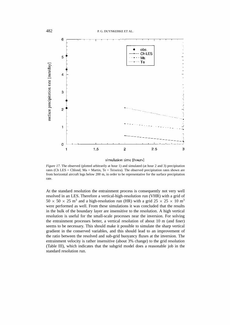
In Figure 17 the instantaneous surface precipitation rates, at hours 2 and 3, forthree model simulations (Ch LES, and the SCMs of Ma and Te) including drizzle

INTERCOMPARISON OF THREE- AND ONE-DIMENSIONAL MODEL SIMULATIONS 479

Figure 14.The observed and simulated liquid water content (Za LES = Zanten, Cu = Cuxart, Le =Lenderink, Ma = Martin, Te = Teixeira) averaged over the third hour, as a function of height (z).The observed liquid water content is the sum of the values derived from the FSSP and260X particleprobes.

are shown. It can clearly be seen that the surface precipitation of the ECMWF SCM(Te) is much higher than the other two models: almost twice as high as the UKMOSCM (Ma) and almost an order of magnitude higher (at hour 3) than the LESmodel. These results seem to support the idea that the ECMWF SCM is precip-itating too much, although a comparison against observations (with large scatter)seem to show that the ECMWF model is more realistic. Moreover, the drizzle isquite important for the liquid water path (LWP) of the cloud. For example, theLES of Chlond (Ch) gives a reduction of about 30% and the SCMs a reduction ofabout 55% in the LWP compared to the run without drizzle. It is clear that there isconsiderable uncertainty in how to parametrize drizzle production in both SCM andLES, whereas the effects of drizzle on cloud life time and evolution are obviouslyimportant to the overall simulation of clouds in a GCM.

480 P. G. DUYNKERKE ET AL.

Figure 15. The observed and simulated buoyancy flux (Za LES = Zanten, Cu = Cuxart, Le =Lenderink, Ma = Martin) averaged over the third hour, as a function of height (z).

5. Discussion and Conclusions

Observations from flight RF06 of the NCAR Electra in a boundary layer with stra-tocumulus (Roode and Duynkerke, 1997) during the First Lagrangian of ASTEXare used to set up an idealized model intercomparison case. For instance, drizzlewas observed but has not been simulated in the basic case. The simulations withdrizzle revealed that this process had only a slight influence (about 10%) on theturbulent fluxes in the boundary layer.

The four LES models predict an entrainment velocity of 1.9± 0.1 cm s−1

compared to an observed value of 1.2± 1 cm s−1 derived from the observed ozonefluxes. The LES modelled entrainment velocity is therefore rather high comparedto the observations. In an LES model part of the entrainment is explicitly resolvedand part of it is parametrized (sub-grid model). At the standard simulation (50×50× 25 m3) of Za, 40% of the total buoyancy flux at the inversion is resolved andthe remainder is subgrid. In the other LES models the resolved part is even smaller.

INTERCOMPARISON OF THREE- AND ONE-DIMENSIONAL MODEL SIMULATIONS 481

Figure 16.The observed and simulated (a) total water content and (b) total water flux (Za LES =Zanten, Cu = Cuxart, Le = Lenderink, Ma = Martin) averaged over the third hour, as a function ofheight (z).

482 P. G. DUYNKERKE ET AL.

Figure 17.The observed (plotted arbitrarily at hour 1) and simulated (at hour 2 and 3) precipitationrates (Ch LES = Chlond, Ma = Martin, Te = Teixeira). The observed precipitation rates shown arefrom horizontal aircraft legs below 200 m, in order to be representative for the surface precipitationrate.

At the standard resolution the entrainment process is consequently not very wellresolved in an LES. Therefore a vertical-high-resolution run (VHR) with a grid of50× 50× 25 m3 and a high-resolution run (HR) with a grid 25× 25× 10 m3

were performed as well. From these simulations it was concluded that the resultsin the bulk of the boundary layer are insensitive to the resolution. A high verticalresolution is useful for the small-scale processes near the inversion. For solvingthe entrainment processes better, a vertical resolution of about 10 m (and finer)seems to be necessary. This should make it possible to simulate the sharp verticalgradient in the conserved variables, and this should lead to an improvement ofthe ratio between the resolved and sub-grid buoyancy fluxes at the inversion. Theentrainment velocity is rather insensitive (about 3% change) to the grid resolution(Table III), which indicates that the subgrid model does a reasonable job in thestandard resolution run.

INTERCOMPARISON OF THREE- AND ONE-DIMENSIONAL MODEL SIMULATIONS 483

From the 1996 intercomparison of working group 1 of the GCSS (Duynkerkeet al., 2000), based on flight 2 (just before the flight we use here) reported byRoode and Duynkerke (1997), we found an LES-derived entrainment velocity of1.3 cm s−1. The main difference between the case described here and the 1996intercomparison is that the jump in total water content at the inversion in that caseis slightly less negative (1qt = −1.1 g kg−1). This indicates that the value of theentrainment velocity is very sensitive (40% change) to the total water jump at theinversion.

All SCMs predict a solid stratocumulus layer with the correct liquid water pro-file. However, the buoyancy flux profile in these models is very poorly represented.The entrainment velocity of the SCMs would indeed be close to the value observedfrom the observations. However, the buoyancy flux in the cloud layer of the SCMsdoes not agree with the observations (Figure 15) and is very sensitive to the en-trainment velocity (Duynkerke et al., 1995). The largest error in the observationsis probably in the estimated value of the ‘observed’ subsidence that is needed toinfer the observed entrainment velocity. In contrast, the measurement error in thebuoyancy flux is rather small. The conclusion therefore is that, because of the goodagreement between the observed and the LES modelled in-cloud buoyancy flux,the entrainment velocities calculated by the LES are reliable.

Because extensive marine stratocumulus clouds are a persistent feature (of theeastern parts of the major ocean basins) it is obvious that the inversion heightmust be almost stationary. This implies a balance between the subsidence and theentrainment velocity:∂h/∂t = we − ws ∼= 0. Because typically the subsidencevelocity changes almost linearly with height we have in a stationary situation thata reduction in the entrainment velocity will lead to a reduction in the boundarylayer depth. From the intercomparison it is concluded that the entrainment velocityin SCMs can be half the value obtained from LES models. In a climate model anerror of a factor two is not acceptable because, given the large-scale subsidence,this means that in steady-state the boundary-layer depth can differ by as much as afactor two.

Observations and model simulations (LES and SCM) show that the micro-physics does not solely influence the radiation but also has direct dynamicalconsequences. The inclusion of drizzle can significantly alter the net transfer ofwater substance and the effect can be comparable to turbulent transport at all levelsin and below the cloud layer. Therefore, the effects of drizzle on cloud lifetime andevolution are obviously important to the overall simulation of clouds in a GCM.From the intercomparison it is clear that there is considerable uncertainty abouthow to parametrize drizzle production in both SCM and LES. This is an area wheremore observations are needed for evaluating model simulations.

484 P. G. DUYNKERKE ET AL.

Acknowledgements

The observational data collected by means of the Electra were provided by Dr.D. H. Lenschow and Ron Ruth of NCAR. We thank NCAR and its sponsor, theNational Science Foundation, allowing us to use the observational data. The in-vestigations were supported by the CEC contract ENV4-CT95-0107 EUCREM(European Cloud Resolving Modelling Programme). M. C. vanZanten acknow-ledges the support received from the National Computing facilities Foundation(NCF) in the form of computer facilities and the Netherlands Geosciences Found-ation (GOA) which is financially aided (grant 750.295.03B) by the NetherlandsOrganization for Scientific Research (NWO).

Appendix A: List of Participants, Affiliations and Model References

Chlond, A., Max-Planck-Institute für Meteorologie (MPI), Bundesstraße 55,D 2000 Hamburg, Germany. Model references: Chlond (1992); Chlond(1994); Luepkes et al. (1989); Luepkes (1991).

vanZanten, M. C., Institute for Marine and Atmospheric Research (IMAU), UtrechtUniversity, Princetonplein 5, 3584 CC Utrecht, The Netherlands. Modelreferences: Cuijpers and Duynkerke (1993); Vreugdenhil and Koren (eds.)(1993); Siebesma and Cuijpers (1995).

Clark, P., Atmospheric Physics Group, Physics Department, UMIST P.O. Box88 Manchester M60 1QD, U.K. Model references: Shutts and Gray (1994);MacVean and Mason (1993).

Cuxart, J. and E. Sanchez, Servicio de Prediccion Numerica, Instituto Nacional deMeteorologia (INM), Apartado 285, 28040 Madrid, Spain. Model references:The Meso-NH Atmospheric Simulation System: Scientific Documentation(1995); Cuxart et al. (1995).

Martin, G., Hadley Centre, U.K. Meteorological Office, London Road, Bracknell,Berkshire, RG12 2SY, U.K. Model references: Cullen (1993); Smith (1990);Smith (1994); Gregory and Rowntree (1990).

Lenderink, G., Royal Netherlands Meteorological Institute (KNMI), P.O. Box 201,3730 AE De Bilt, Wilhelminalaan 10, The Netherlands. Model references:Brinkop and Roeckner (1995); Roeckner et al. (1996).

Teixeira, J. European Centre for Medium Range Weather Forecasting (ECMWF),Shinfield Park, Reading, Berkshire RG2 9AX, U.K. Model references: Louiset al. (1982); Tiedtke (1993); Tiedtke (1989), Beljaars and Betts (1993).

INTERCOMPARISON OF THREE- AND ONE-DIMENSIONAL MODEL SIMULATIONS 485

References

ASTEX operations plan. Prepared by the Fire Project Office and ASTEX Working Group. March1992. Obtainable from: FIRE Project Manager, Mail Stop 483, NASA Langley Research Center,Hampton, VA, 23665-5225, U.S.A.

Albrecht, B. A., Bretherton, C. S., Johnson, D., Schubert, W. H., and Frisch, A. S.: 1995, ‘TheAtlantic Stratocumulus Transition Experiment-ASTEX’,Bull. Amer. Meteorol. Soc.76, 889–904.

Bechtold, P., Krueger, S. K., Lewellen, W. S., van Meijgaard, E., Moeng, C.-H., Randall, D. A.,van Ulden, A., and Wang, S.: 1996, ‘Modeling a Stratocumulus-Topped PBL: IntercomparisonsAmong Different 1D Codes and with LES’,Bull. Amer. Meteoreol. Soc.77, 2033–2042.

Beljaars, A. C. M. and Betts, A. K.: 1993, ‘Validation of the Boundary Layer Representation in theECMWF Model’, ECMWF Seminar proceedings 7–11 September 1992, Validation of modelsover Europe, Vol. II, 159–196.

Bower, K. N. and Choularton, T. W.: 1992, ‘A Parametrization of the Effective Radius of Ice FreeClouds for Use in Global Climate’,Atmos. Res.27, 305–339.

Brinkop, S. and Roeckner, E.: 1995, ‘Sensitivity of a General Circulation Model to Parameterizationsof Cloud-Turbulence Interactions in the Atmospheric Boundary Layer’,Tellus47A, 197–220.

Chlond, A.: 1992, ‘Three-Dimensional Simulation of Cloud Street Development during a Cold AirOutbreak’,Boundary-Layer Meteorol.58, 161–200.

Chlond, A.: 1994, ‘Locally Modified Version of Bott’s Advection Scheme’,Mon. Wea. Rev.122,111–125.

Cuijpers, J. W. M. and Duynkerke, P. G.: 1993, ‘Large-Eddy Simulation of Trade-Wind CumulusClouds’,J. Atmos. Sci.50, 3894–3908.

Cullen, M. J. P.: 1993, ‘The Unified Forecast/Climate Model’,Meteorol. Magazine122, 81–94.Cuxart, J., Bougeault, P., and Redelsperger, J.-L.: 1995, ‘Turbulence Closure for a Non-Hydrostatic

Model’, in Proceedings of 11th Symposium on Boundary Layers and Turbulence, paper 14.9, pp.409–412.

Deardorff, J. W.: 1976, ‘On the Entrainment Rate of Stratocumulus-Topped Mixed Layer’,Quart. J.Roy. Meteorol. Soc.102, 563–582.

DeLaat, A. T. J. and Duynkerke, P. G.: 1998, ‘Analysis of ASTEX-Stratocumulus Observational DataUsing a Mass Flux Approach’,Boundary-Layer Meteorol.86, 63–87.

de Roode, S. R. and Duynkerke, P. G.: 1997, ‘Observed Lagrangian Transition of Stratocumulus intoCumulus during ASTEX: Mean State and Turbulence Structure’,J. Atmos. Sci.54, 2157–2173.

Driedonks, A. G. M. and Duynkerke, P. G.: 1989, ‘Current Problems in the Stratocumulus-ToppedAtmospheric Boundary Layer’,Boundary-Layer Meteorol.46, 275–304.

Duynkerke P. G., Zhang, H., and Jonker, P. J.: 1995, ‘Microphysical and Turbulent Structure ofNocturnal Stratocumulus as Observed during ASTEX’,J. Atmos. Sci. 52, 2763–2777.

Duynkerke, P. G., Jonker, P. J., Bechtold, P., Chlond, A., Cuijpers, J. W. M., Cuxart, J., Feingold, G.,Lewellen, D. C., Lock, A., Meijgaard, E., Moeng, C.-H., Teixeira, J., Stevens, B., and Wyant,M.: 2000, ‘Simulation of a Stratocumulus-Topped Atmospheric Boundary Layer: A Comparisonof Models and Observations’, to be submitted toBull. Amer. Meteoreol. Soc.

Gerber, H.: 1996, ‘Microphysics of Marine Stratocumulus Clouds with Two Drizzle Modes’,J.Atmos. Sci.53, 1649–1662

Gregory, D. and Rowntree, P. R.: 1990, ‘A Mass Flux Convection Scheme with Representation ofCloud Ensemble Characteristics and Stability-Dependent Closure’,Mon. Wea. Rev.118, 1483–1506.

Hignett, P.: 1991, ‘Observations of the Diurnal Variation in a Cloud-Capped Marine BoundaryLayer’, J. Atmos. Sci.48, 1474–1482.

Jonker, H. J. J., Cuijpers, J. W. M., and Duynkerke, P. G.: 1999, ‘Mesoscale Fluctuations in ScalarsGenerated by Boundary Layer Convection’,J. Atmos. Sci.56, 801–808.

486 P. G. DUYNKERKE ET AL.

Lenderink, G. and Holtslag, A. A. M.: 1998, ‘Evaluation of the Kinetic Energy Approach for Mod-elling Turbulent Fluxes in Stratocumulus’, KNMI preprints No. 98-11, 24 pp. (Available fromKNMI, P.O. Box 201, 3730 AE De Bilt, The Netherlands.)

Lilly, D.K.: 1967, ‘The Representation of Small-Scale Turbulence in Numerical Simulation Experi-ments’, inProc. IBM Scientific Computing Symp. on Environmental Science, Yorktown Heights,NY, pp. 195–210.

Lock, A. P. and MacVean, M. K.: 1999, ‘The Parametrization of Entrainment Driven by SurfaceHeating and Cloud-Top Cooling’,Quart. J. Roy. Meteorol. Soc.125, 271–299.

Louis, J. F., Tiedtke M., and Geleyn, J. F.: 1982, ‘A Short History of the Operational PBL-Parametrization at ECMWF’, Workshop on Boundary Layer Parametrization, November 1981,ECMWF, Reading, U.K.

Luepkes, C., Beheng, K. D., and Doms, G.: 1989, ‘A Parameterization Scheme for SimulatingCollision/Coalescence of Water Drops’,Beitr. Phys. Atmosph.62, 289–306.

Luepkes, C.: 1991, ‘Untersuchung zur Parameterisierung der Koagulation niederschlagsbildenderTropfen’, Verlag Dr. Kovacs, Hamburg, 156 pp.

MacVean M. K. and Mason, P. J.: 1993, ‘A Numerical Investigation of the Criterion for Cloud-Top Entrainment through Small Scale Mixing and its Parametrization in Numerical Models’,J.Atmos. Sci.50, 2481–2495.

Moeng, C.-H., Cotton, W. R., Bretherton, C. S., Chlond, A., Khairoutdinov, M., Krueger, S., Lewel-len, W. S., MacVean, M. K., Pasquier, J. R. M., Rand, H. A., Siebesma, A. P., Sykes, R. I.,and Stevens, B.: 1996, ‘Simulation of a Stratocumulus-Topped PBL: Intercomparison amongDifferent Numerical Codes’,Bull. Amer. Meteorol. Soc.77, 261–278.

Nicholls, S.: 1984, ‘The Dynamics of Stratocumulus: Aircraft Observations and Comparison with aMixed-Layer Model’,Quart. J. Roy. Meteorol. Soc.110, 783–820.

Nicholls, S.: 1989, ‘The Structure of Radiatively Driven Convection in Stratocumulus’,Quart. J.Roy. Meteorol. Soc.115, 487–511.

Paluch, I. R. and Lenschow, D. H.: 1991, ‘Stratiform Cloud Formation in the Marine BoundaryLayer’, J. Atmos. Sci.48, 2141–2158.

Randall, D. A., Shao, Q., Moeng, C.H.: 1992, ‘A Second-Order Bulk Boundary Layer Model’,J.Atmos. Sci.49, 1903–1923.

Roeckner, E., Arpe, K., Bengtsson, L., Christoph, M., Claussen, M., Düminil, L., Esch, M., Gior-getta, M., Schlese, U., and Schulzweida, U.: 1996, ‘The Atmospheric General Circulation ModelECHAM-4: Model Description and Simulation of Present-Day Climate’, Max-Planck-Institut fürMeteorologie Report 218.

Rogers, R. R.: 1979,A Short Course in Cloud Physics, 2nd edition, Pergamon Press, 235 pp.Shutts, G. J. and Gray, M. E. B.: 1994, ‘A Numerical Modelling Study of the Geostrophic Adjustment

Process Following Deep Convection’,Quart. J. Roy. Meteorol. Soc.120, 1145–1178.Siebesma, A. P. and Cuijpers, J. W. M.: 1995, ‘Evaluation of Parametric Assumptions for Shallow

Cumulus Convection’,J. Atmos. Sci.52, 650–666.Smagorinsky, J.: 1963: ‘General Circulation Experiments with the Primitive Equations’,Mon. Wea.

Rev.91, 99–165.Smith, R. N. B: 1990, ‘A Scheme for Predicting Layer Clouds and their Water Content in a General

Circulation Model’,Quart. J. Roy. Meteorol. Soc.116, 435–460.Smith, R. N. B.: 1994, ‘Experience and Developments with Layer Cloud and Boundary Layer

Mixing Scheme in the UKMO Unified Model’, ECMWF Workshop: Parametrization of theCloud-Topped Boundary Layer, 8–11 June 1993. ECMWF, Reading, U.K., 429 pp.

Sommeria, G.: 1976, ‘Three-Dimensional Simulation of Turbulent Processes in an UndisturbedTrade Wind Boundary Layer’,J. Atmos. Sci.33, 216–241.

Sommeria, G. and Deardorff, J. W.: 1977, ‘Subgrid-Scale Condensation in Models of Nonprecipitat-ing Clouds’,J. Atmos. Sci.33, 344–355.

INTERCOMPARISON OF THREE- AND ONE-DIMENSIONAL MODEL SIMULATIONS 487

Stage, S. A. and Businger, J. A.: 1981: ‘A Model for Entrainment into a Cloud-Topped MarineBoundary Layer. Part I: Model Description and Application to a Cold Air Outbreak Episode’,J.Atmos. Sci.38, 2213–2229.

Stull, R. B.: 1988, ‘An Introduction to Boundary Layer Meteorology’, Kluwer Academic Publishers,Dordrecht, 666 pp.

The Meso-NH Atmospheric Simulation System: Scientific Documentation, Book 1, 1995, Chapters13 (turbulence scheme) and 14 (subgrid condensation scheme), Meteo-France and CNRS. Sev-eral authors, edited by Philippe Bougeault. Available from Meteo-France, CNRM/GMME, AV.G.Coriolis 42, 31057 Toulouse CEDEX. France.

Tiedtke, M.: 1989, ‘A Comprehensive Mass Flux Scheme for Cumulus Parametrization in LargeScale Models’,Mon. Wea. Rev.117, 1779–1800.

Tiedtke, M.: 1993, ‘Representation of Clouds in Large-Scale Models’,Mon. Wea. Rev.121, 3040–3061.

vanZanten, M. C., Duynkerke, P. G., and Cuijpers, J. W. M.: 1999, ‘Entrainment in ConvectiveBoundary Layers’,J. Atmos. Sci.56, 813–828.

Vreugdenhil, C. B. and Koren, B. (eds.): 1993,Notes on Numerical Fluid Mechanics, Volume45, Numerical Methods for Advection-Diffusion Problems, Vieweg, Braunschweig/Wiesbaden,Germany, 373 pp.