Model intercomparison in the Mediterranean: MEDMEX simulations of the seasonal cycle

Model intercomparison in the Mediterranean: MEDMEX

simulations of the seasonal cycle

J.-M. Beckers a,*, M. Rixen a, P. Brasseur b, J.-M. Brankart b, A. Elmoussaoui a,M. Crepon c, Ch. Herbaut c, F. Martel d, F. Van den Berghe d, L. Mortier c,

A. Lascaratos e, P. Drakopoulos f, G. Korres e, K. Nittis e, N. Pinardi g, E. Masetti h,S. Castellari i, P. Carini i, J. Tintore j, A. Alvarez k, S. Monserrat j, D. Parrilla j,

R. Vautard l, S. Speichm

aUniversity of Liege, GHER, Sart-Tilman B5, B-4000 Liege, BelgiumbLEGI-UMR, 5519 du CNRS-Equipe MEOM-BP53X, F-38041 Grenoble Cedex, France

cLaboratoire d’Oceanographie Dynamique et de Climatologie, Universite Pierre et Marie Curie Tour 26, Boite 100 4,

place Jussieu, 75252 Paris Cedex 05, FrancedCETIIS, Bat. D, Allee de Beaumanoir 30, Av. Malacrida, 13100 Aix en Provence, France

eOcean Physics Group, Department of Applied Physics University Campus, Building PHYS-5 Athens, GR-15784 GreecefInstitute of Marine Biology of Crete, P.O. Box 2214 Heraklion 71003 Crete, GreecegDepartment of Physics, Bologna University, Viale Berti Pichat 6/2, Bologna, Italy

hISAO, Via P. Gobetti, 101 C.A.P., 40129 Bologna, ItalyiISAO-CNR Via Gobetti 101, 40129 Bologna, Italy

jIMEDEA (CSIC-UIB) Edifici Mateu Orfila i Rotger Campus universitari, E-07071 Palma, SpainkSACLANT Undersea Research Centre Viale San Bartolomeo, 400 19138 La Spezia, Italy

lL.M.D. Ecole Polytechnique Ecole Normale Superieure Universite de Paris, 6 F 91128 Palaiseau Cedex, FrancemLaboratoire de Physique des Oceans Universite de Bretagne Occidentale UFR Sciences-6,

Avenue Le Gorgeu B.P. 809 29285 Brest Cedex, France

Received 20 February 2001; accepted 10 August 2001

Abstract

The simulation of the seasonal cycle in the Mediterranean by several primitive equation models is presented. All

models were forced with the same atmospheric data, which consists in either a monthly averaged wind-stress with sea

surface relaxation towards monthly mean sea surface temperature and salinity fields, or by daily variable European Centre

for Medium Range Weather Forecast (ECMWF) reanalysed wind-stress and heat fluxes. In both situations models used the

same grid resolution. Results of the modelling show that the model behaviour is similar when the most sensitive parameter,

vertical diffusion, is calibrated properly. It is shown that an unrealistic climatic drift must be expected when using monthly

averaged forcing functions. When using daily forcings, drifts are modified and more variability observed, but when

performing an EOF analysis of the sea surface temperature, it is shown that the basic cycle, represented similarly by the

0924-7963/02/$ - see front matter D 2002 Elsevier Science B.V. All rights reserved.

PII: S0924 -7963 (02 )00060 -X

* Corresponding author. National Fund for Scientific Research, University of Liege, GHER, Sart-Tilman B5, B-4000 Liege, Belgium. Tel.:

+32-4-366-33-58; fax: +32-4-366-23-55.

E-mail address: [email protected] (J.-M. Beckers).

www.elsevier.com/locate/jmarsys

Journal of Marine Systems 33–34 (2002) 215–251

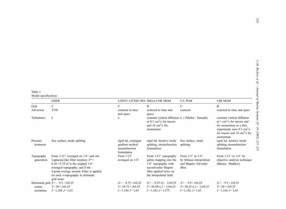
Table 1

Model specifications

GHER LODYC-CETIIS OPA IMGA-CNR MOM UA POM UIB MOM

Grid C C B C B

Advection TVD centered in time

and space

centered in time and

space

centered centered in time and space

Turbulence k k constant vertical diffusion

at 0.3 cm2/s for tracers

and 10 cm2/s for

momentum

k, l (Mellor–Yamada) constant vertical diffusion

at 1 cm2/s for tracers and

for momentum in a first

experiment, now 0.3 cm2/s

for tracers and 10 cm2/s for

momentum

Pressure

treatment

free surface, mode splitting rigid lid, conjugate

gradient method

streamfunction

formulation

rigid lid, iterative mode

splitting, streamfunction

formulation

free surface, mode

splitting

rigid lid, iterative mode

splitting streamfunction

formulation

Topography

generation

From 1/12j averaged on 1/4j and one

Laplacian-like filter iteration: h* =

0.3h+ 0.7h (h is the original 1/4javeraged topography, and h the

4-point average around. Filter is applied

on each j-topography to eliminate

grid noise.

From 1/12javeraged on 1/4j.

From 1/12j topography

spline mapping into the

1/4j topography with

second-order Shapiro

filter applied twice on

the interpolated field.

From 1/2j to 1/4jby bilinear interpolation

and Shapiro 3rd-order

filter.

From 1/12j to 1/4j by

objective analysis technique

(Barnes–Maddox).

Horizontal grid X =� 9.5 + I*0.25 X =� 9.75 + I*0.25 X =� 9.25+(I� 1)*0.25 X=� 9.5 + I*0.25 X =� 9.5 + I*0.25

coarse Y= 30 + J*0.25 Y= 29.75 + J*0.25 Y= 30.50+( J� 1)*0.25 Y= 30.25+( J� 1)*0.25 Y= 30 + J*0.25

resolution I = 1,184 J= 1,63 I = 1,184 J = 1,63 I = 1,182 J= 1,575 I = 1,182 J= 1,63 I = 1,184 J= 1,63

J.-M.Beckers

etal./JournalofMarin

eSystem

s33–34(2002)215–251

216

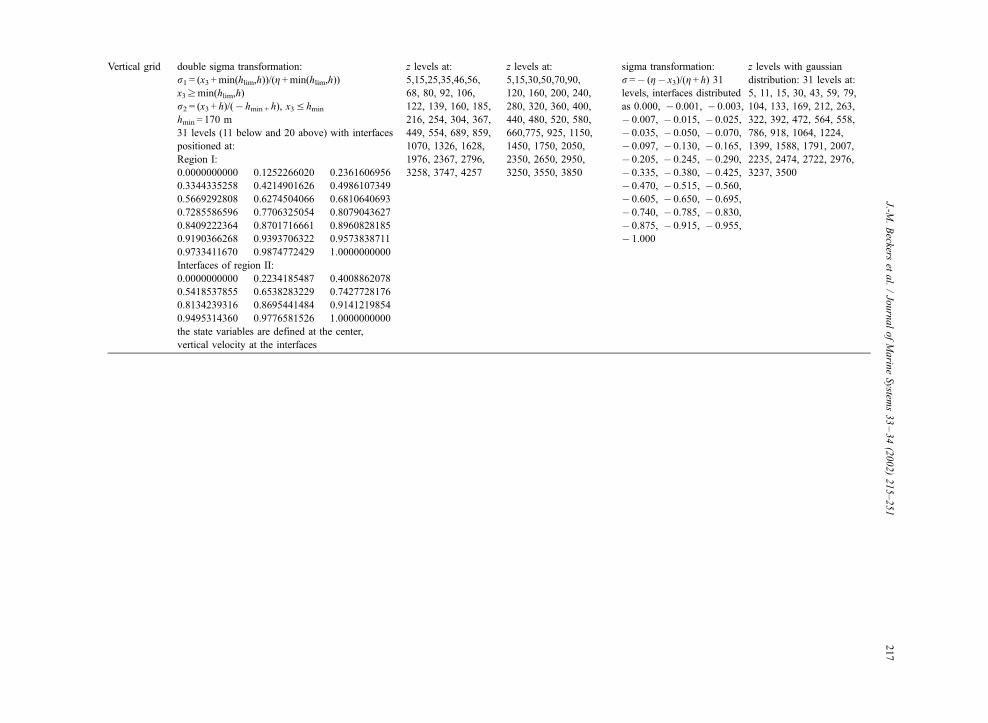
Vertical grid double sigma transformation: z levels at: z levels at: sigma transformation: z levels with gaussian

r1 = (x3 +min(hlim,h))/(g+min(hlim,h)) 5,15,25,35,46,56, 5,15,30,50,70,90, r=� (g� x3)/(g+ h) 31 distribution: 31 levels at:

x3zmin(hlim,h) 68, 80, 92, 106, 120, 160, 200, 240, levels, interfaces distributed 5, 11, 15, 30, 43, 59, 79,

r2 = (x3 + h)/(� hmin + h), x3V hmin 122, 139, 160, 185, 280, 320, 360, 400, as 0.000, � 0.001, � 0.003, 104, 133, 169, 212, 263,

hmin = 170 m 216, 254, 304, 367, 440, 480, 520, 580, � 0.007, � 0.015, � 0.025, 322, 392, 472, 564, 558,

31 levels (11 below and 20 above) with interfaces

positioned at:

449, 554, 689, 859,

1070, 1326, 1628,

660,775, 925, 1150,

1450, 1750, 2050,

� 0.035, � 0.050, � 0.070,

� 0.097, � 0.130, � 0.165,

786, 918, 1064, 1224,

1399, 1588, 1791, 2007,

Region I: 1976, 2367, 2796, 2350, 2650, 2950, � 0.205, � 0.245, � 0.290, 2235, 2474, 2722, 2976,

0.0000000000 0.1252266020 0.2361606956 3258, 3747, 4257 3250, 3550, 3850 � 0.335, � 0.380, � 0.425, 3237, 3500

0.3344335258 0.4214901626 0.4986107349 � 0.470, � 0.515, � 0.560,

0.5669292808 0.6274504066 0.6810640693 � 0.605, � 0.650, � 0.695,

0.7285586596 0.7706325054 0.8079043627 � 0.740, � 0.785, � 0.830,

0.8409222364 0.8701716661 0.8960828185 � 0.875, � 0.915, � 0.955,

0.9190366268 0.9393706322 0.9573838711 � 1.000

0.9733411670 0.9874772429 1.0000000000

Interfaces of region II:

0.0000000000 0.2234185487 0.4008862078

0.5418537855 0.6538283229 0.7427728176

0.8134239316 0.8695441484 0.9141219854

0.9495314360 0.9776581526 1.0000000000

the state variables are defined at the center,

vertical velocity at the interfaces

J.-M.Beckers

etal./JournalofMarin

eSystem

s33–34(2002)215–251

217

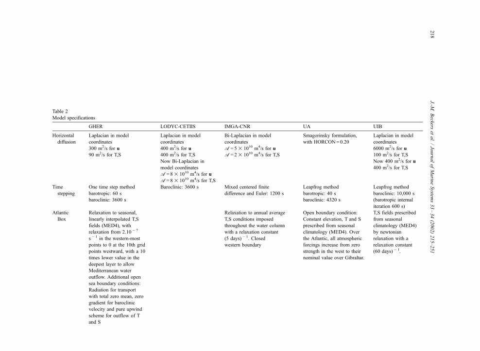
Table 2

Model specifications

GHER LODYC-CETIIS IMGA-CNR UA UIB

Horizontal

diffusion

Laplacian in model

coordinates

Laplacian in model

coordinates

Bi-Laplacian in model

coordinates

Smagorinsky formulation,

with HORCON=0.20

Laplacian in model

coordinates

300 m2/s for u 400 m2/s for u A= 5� 1010 m4/s for u 6000 m2/s for u

90 m2/s for T,S 400 m2/s for T,S A= 2� 1010 m4/s for T,S 100 m2/s for T,S

Now Bi-Laplacian in

model coordinates

Now 400 m2/s for u

400 m2/s for T,S

A= 8� 1010 m4/s for u

A= 8� 1010 m4/s for T,S

Time One time step method Baroclinic: 3600 s Mixed centered finite Leapfrog method Leapfrog method

stepping barotropic: 60 s difference and Euler: 1200 s barotropic: 40 s baroclinic: 10,000 s

baroclinic: 3600 s baroclinic: 4320 s (barotropic internal

iteration 600 s)

Atlantic

Box

Relaxation to seasonal,

linearly interpolated T,S

fields (MED4), with

relaxation from 2.10� 7

s� 1 in the western-most

points to 0 at the 10th grid

points westward, with a 10

times lower value in the

deepest layer to allow

Mediterranean water

outflow. Additional open

sea boundary conditions:

Radiation for transport

with total zero mean, zero

gradient for baroclinic

velocity and pure upwind

scheme for outflow of T

and S

Relaxation to annual average

T,S conditions imposed

throughout the water column

with a relaxation constant

(5 days)� 1. Closed

western boundary

Open boundary condition:

Constant elevation, T and S

prescribed from seasonal

climatology (MED4). Over

the Atlantic, all atmospheric

forcings increase from zero

strength in the west to their

nominal value over Gibraltar.

T,S fields prescribed

from seasonal

climatology (MED4)

by newtonian

relaxation with a

relaxation constant

(60 days) � 1.

J.-M.Beckers

etal./JournalofMarin

eSystem

s33–34(2002)215–251

218

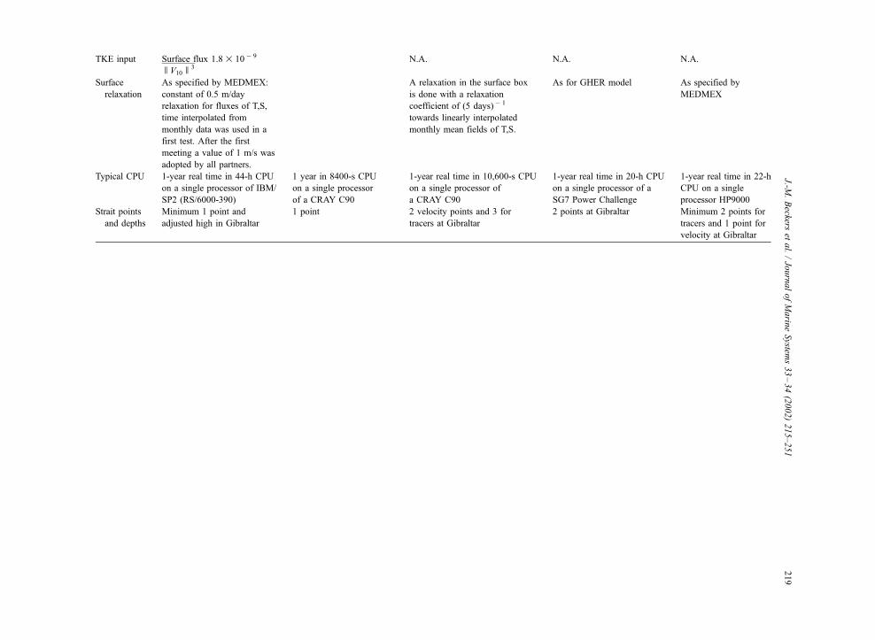
TKE input Surface flux 1.8� 10� 9

OV10O3

N.A. N.A. N.A.

Surface

relaxation

As specified by MEDMEX:

constant of 0.5 m/day

relaxation for fluxes of T,S,

time interpolated from

monthly data was used in a

first test. After the first

meeting a value of 1 m/s was

adopted by all partners.

A relaxation in the surface box

is done with a relaxation

coefficient of (5 days)� 1

towards linearly interpolated

monthly mean fields of T,S.

As for GHER model As specified by

MEDMEX

Typical CPU 1-year real time in 44-h CPU

on a single processor of IBM/

SP2 (RS/6000-390)

1 year in 8400-s CPU

on a single processor

of a CRAY C90

1-year real time in 10,600-s CPU

on a single processor of

a CRAY C90

1-year real time in 20-h CPU

on a single processor of a

SG7 Power Challenge

1-year real time in 22-h

CPU on a single

processor HP9000

Strait points

and depths

Minimum 1 point and

adjusted high in Gibraltar

1 point 2 velocity points and 3 for

tracers at Gibraltar

2 points at Gibraltar Minimum 2 points for

tracers and 1 point for

velocity at Gibraltar

J.-M.Beckers

etal./JournalofMarin

eSystem

s33–34(2002)215–251

219

models, consists of the seasonal cycle which accounts for more than 90% of its variability. D 2002 Elsevier Science B.V.

All rights reserved.

Keywords: Mediterranean; MEDMEX; Seasonal cycle

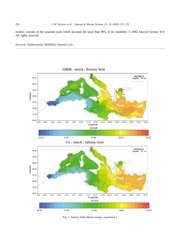
Fig. 1. Salinity fields March average, experiment I.

J.-M. Beckers et al. / Journal of Marine Systems 33–34 (2002) 215–251220

1. Introduction

The present paper is an attempt to give a flavour of

results obtained during a project aimed at promoting

model intercomparison in the Mediterranean Sea.

Prior to the MEDMEX project, extensive model-

ling exercises had been performed in the Medi-

terranean Sea (EROS2000, EUROMODEL and

MERMAIDS projects with models of Beckers,

1991; EUROMODEL group, 1995; MERMAIDS,

1998), but coordination and comparison between the

different modelling aspects was sporadic. Thus, there

already exists a series of studies devoted to the

modelling of the Mediterranean Sea: Becker (1991)

used a 15-km resolution model in the Western Med-

iterranean to calculate the seasonal cycle, including a

relaxation towards MODB (Brasseur et al., 1996)

temperature and salinity fields; Zavatarelli and Mellor

(1995) used the POM model with curvilinear coor-

dinates on the whole Mediterranean; the OPA model

was applied successively to the western Mediterra-

nean and the entire basin (Herbaut et al., 1996, 1998);

the GFDL model MOM was implemented on the

whole Mediterranean using interactive air–sea fluxes.

Haines and Wu (1998) and Roussenov et al. (1995)

used the GFDL model with surface relaxation fluxes,

while Alvarez et al. (1994) introduced the so-called

Neptune effect into the MOM model applied to the

Mediterranean. The different approaches to the mod-

elling are still going on. Rather than working on

models with resolutions unable to properly resolve

the radius of deformation (25 km in the Mediterra-

nean), most models currently in use are working at a

1/8j scale (Demirov and Pinardi, 2002; Stratford and

Haines, 2002) with emphasis on interannual variations

rather than seasonal cycles. However, when the inter-

comparison was started, it was found necessary to

compare the different models on a common basis, in

order to provide some estimates on the errors and the

most sensitive parameters one could expect for the

different models. This is why a formal group was

created in which the different modellers would sys-

tematically compare their models, which could help

improve models and understand their behaviours.

The results of the so developed MEDMEX experi-

ment are described hereafter. Updated information and

data can be found at: http://modb.oce.ulg.ac.be/MED-

MEX.

Model intercomparison already has a relatively

long tradition in atmospheric modelling (see for

example CMIP http://www.pcmdi.llnl.gov/covey/

cmip/diagsub.html and the AMIP project (Gates et

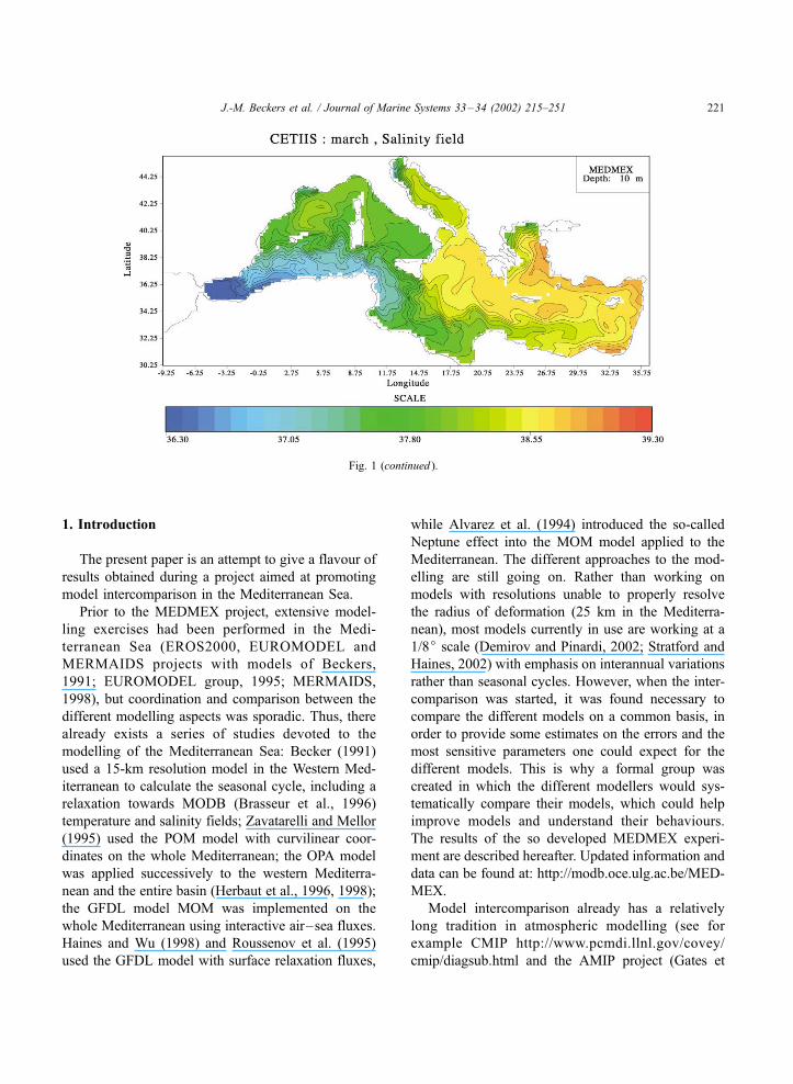
Fig. 1 (continued ).

J.-M. Beckers et al. / Journal of Marine Systems 33–34 (2002) 215–251 221

al., 1999)), but in ocean sciences, model intercompar-

ison has not been widely used, partly because of the

lack of models applied to the same problem, partly

because of computational constraints or lack of data

for control.

Here we will not intercompare on purely mathe-

matical aspects, e.g. on turbulent closure schemes as

done in Davies and Xing (1995), or on a specific

numerical aspect as in Baptista et al. (1995) and James

(1996). A more general model test situation is chosen,

excluding academic test cases, e.g. Røed et al. (1995),

Slørdal et al. (1994) or industrial validation of numer-

ical codes (Dee, 1995). A comparison in more complex

situations was recently done for coastal ocean models

(Haidvogel and Beckmann, 1998), highlighting the

difficulty of models to extract small residual signals

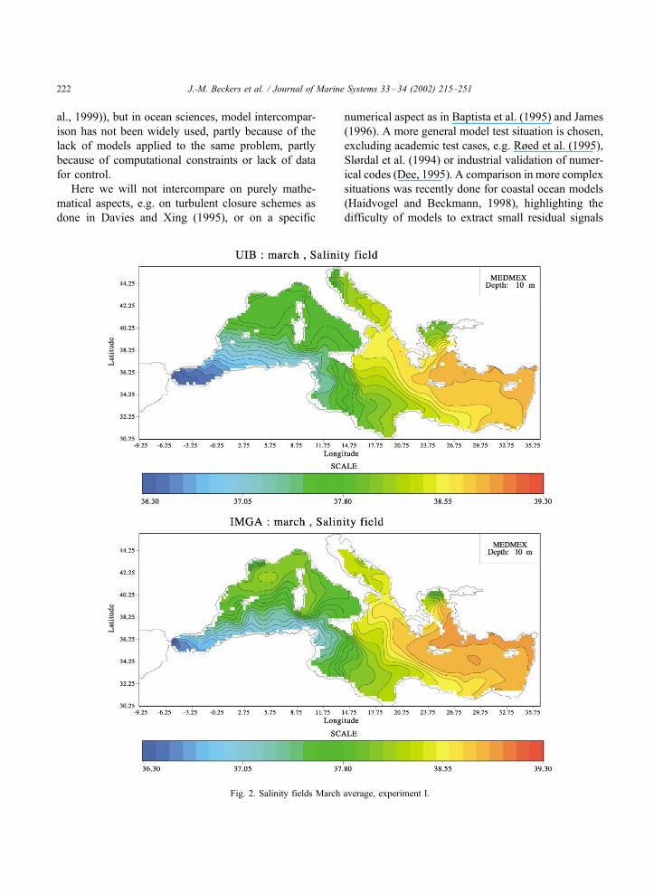
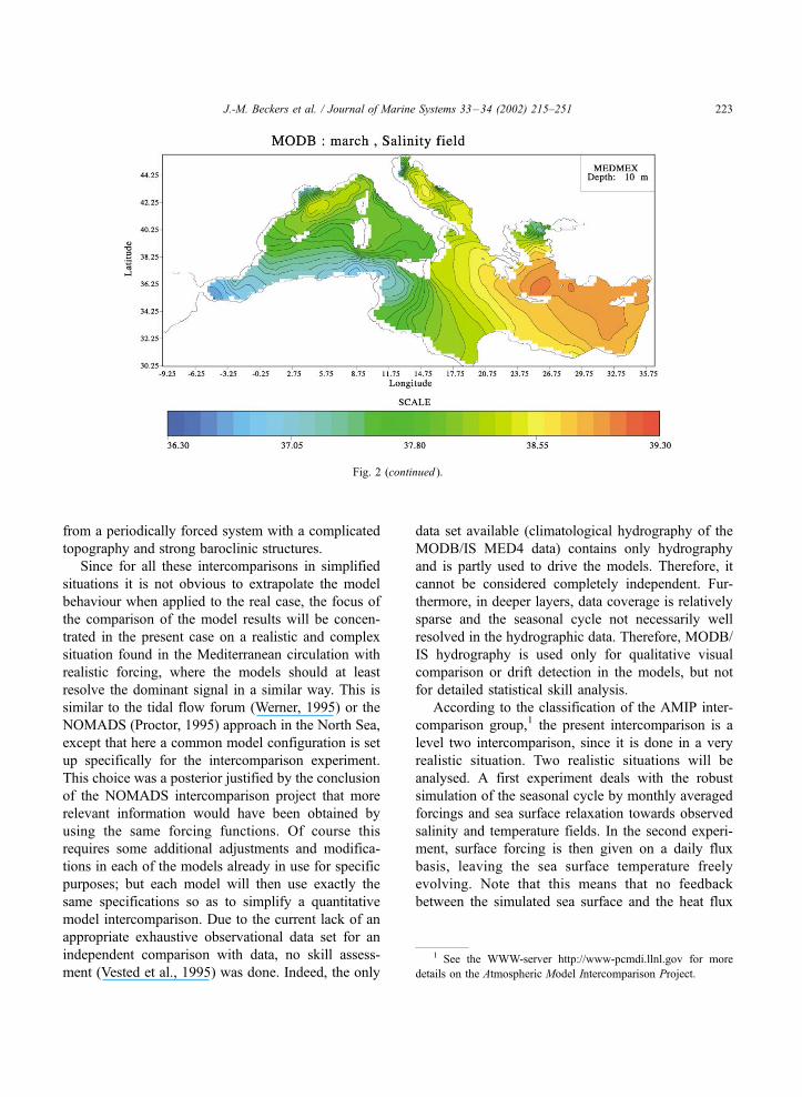
Fig. 2. Salinity fields March average, experiment I.

J.-M. Beckers et al. / Journal of Marine Systems 33–34 (2002) 215–251222

from a periodically forced system with a complicated

topography and strong baroclinic structures.

Since for all these intercomparisons in simplified

situations it is not obvious to extrapolate the model

behaviour when applied to the real case, the focus of

the comparison of the model results will be concen-

trated in the present case on a realistic and complex

situation found in the Mediterranean circulation with

realistic forcing, where the models should at least

resolve the dominant signal in a similar way. This is

similar to the tidal flow forum (Werner, 1995) or the

NOMADS (Proctor, 1995) approach in the North Sea,

except that here a common model configuration is set

up specifically for the intercomparison experiment.

This choice was a posterior justified by the conclusion

of the NOMADS intercomparison project that more

relevant information would have been obtained by

using the same forcing functions. Of course this

requires some additional adjustments and modifica-

tions in each of the models already in use for specific

purposes; but each model will then use exactly the

same specifications so as to simplify a quantitative

model intercomparison. Due to the current lack of an

appropriate exhaustive observational data set for an

independent comparison with data, no skill assess-

ment (Vested et al., 1995) was done. Indeed, the only

data set available (climatological hydrography of the

MODB/IS MED4 data) contains only hydrography

and is partly used to drive the models. Therefore, it

cannot be considered completely independent. Fur-

thermore, in deeper layers, data coverage is relatively

sparse and the seasonal cycle not necessarily well

resolved in the hydrographic data. Therefore, MODB/

IS hydrography is used only for qualitative visual

comparison or drift detection in the models, but not

for detailed statistical skill analysis.

According to the classification of the AMIP inter-

comparison group,1 the present intercomparison is a

level two intercomparison, since it is done in a very

realistic situation. Two realistic situations will be

analysed. A first experiment deals with the robust

simulation of the seasonal cycle by monthly averaged

forcings and sea surface relaxation towards observed

salinity and temperature fields. In the second experi-

ment, surface forcing is then given on a daily flux

basis, leaving the sea surface temperature freely

evolving. Note that this means that no feedback

between the simulated sea surface and the heat flux

Fig. 2 (continued ).

1 See the WWW-server http://www-pcmdi.llnl.gov for more

details on the Atmospheric Model Intercomparison Project.

J.-M. Beckers et al. / Journal of Marine Systems 33–34 (2002) 215–251 223

calculation is present, which is a more difficult sit-

uation to handle than the interactive flux forcing that

includes a stabilising feedback between simulated sea

surface temperature and calculated heat flux.

In Section 2, we will outline the setup used for the

model intercomparison. Results will then be presented

in Sections 3 and 4.

2. Setup of the comparison

The model intercomparison was based on the idea

that the model should run in such a way that forcing

data are identical when possible, in order to avoid any

interpretation problem arising from using different

forcing functions (a situation which arose in an

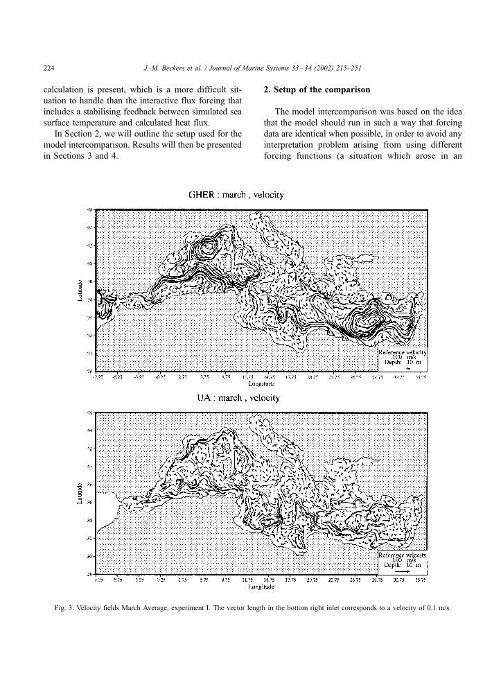
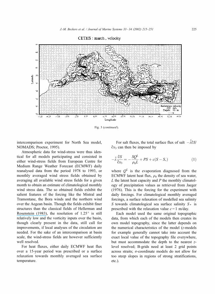
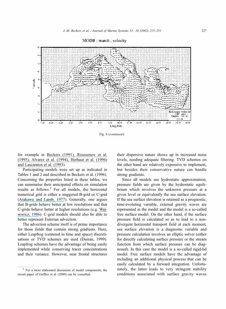
Fig. 3. Velocity fields March Average, experiment I. The vector length in the bottom right inlet corresponds to a velocity of 0.1 m/s.

J.-M. Beckers et al. / Journal of Marine Systems 33–34 (2002) 215–251224

intercomparison experiment for North Sea model,

NOMADS; Proctor, 1995).

Atmospheric data for wind-stress were thus iden-

tical for all models participating and consisted in

either wind-stress fields from European Centre for

Medium Range Weather Forecast (ECMWF) daily

reanalysed data from the period 1978 to 1993, or

monthly averaged wind stress fields obtained by

averaging all available wind stress fields for a given

month to obtain an estimate of climatological monthly

wind stress data. The so obtained fields exhibit the

salient features of the forcing like the Mistral and

Tramontane, the Bora winds and the northern wind

over the Aegean basin. Though the fields exhibit finer

structures than the classical fields of Hellerman and

Rosenstein (1983), the resolution of 1.25j is still

relatively low and the vorticity inputs over the basin,

though clearly present in the data, still call for

improvements, if local analyses of the circulation are

needed. For the sake of an intercomparison at basin

scale, the wind-stress fields are however sufficiently

well resolved.

For heat fluxes, either daily ECMWF heat flux

over a 15-year period was prescribed or a surface

relaxation towards monthly averaged sea surface

temperature.

For salt fluxes, the total surface flux of salt �kqS/qx3 can then be imposed by

�kqSqx3

¼ � SQL

q0Lþ PS þ cðS � S�Þ ð1Þ

where QL is the evaporation diagnosed from the

ECMWF latent heat flux, q0 the density of sea water,

L the latent heat capacity and P the monthly climatol-

ogy of precipitation values as retrieved from Jaeger

(1976). This is the forcing for the experiment with

daily forcings. For climatological monthly averaged

forcings, a surface relaxation of modelled sea salinity

S towards climatological sea surface salinity S * is

prescribed with the relaxation value c = 1 m/day.

Each model used the same original topographic

data, from which each of the models then creates its

own model topography, since the latter depends on

the numerical characteristics of the model (z-models

for example generally cannot take into account the

exact local value of the topography file everywhere,

but must accommodate the depth to the nearest z-

level resolved; B-grids need at least 2 grid points

across straits; r-coordinate models do not allow for

too steep slopes in regions of strong stratifications,

etc.).

Fig. 3 (continued ).

J.-M. Beckers et al. / Journal of Marine Systems 33–34 (2002) 215–251 225

3. General circulation simulated by a monthly

mean atmospheric forcing, experiment I

The first MEDMEX modelling experiment (called

experiment I hereafter) was set up to study the

behaviour of the models when forced by the classical

perpetual year approach, repeating each year the

atmospheric data of a monthly averaged atmosphere,

including sea surface relaxation of temperature and

salinity towards climatological monthly means. The

models participating in the exercise were those ini-

tially used in EU projects MERMAIDS (Pinardi,

1995) and EUROMODEL (Crepon and Martel,

1995). Individual model descriptions can be found

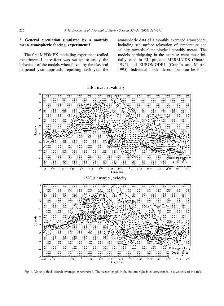
Fig. 4. Velocity fields March Average, experiment I. The vector length in the bottom right inlet corresponds to a velocity of 0.1 m/s.

J.-M. Beckers et al. / Journal of Marine Systems 33–34 (2002) 215–251226

for example in Beckers (1991), Roussenov et al.

(1995), Alvarez et al. (1994), Herbaut et al. (1996)

and Lascaratos et al. (1993).

Participating models were set up as indicated in

Tables 1 and 2 and described in Beckers et al. (1996).

Concerning the properties listed in these tables, we

can summarise their anticipated effects on simulation

results as follows.2 For all models, the horizontal

numerical grid is either a staggered B-grid or C-grid

(Arakawa and Lamb, 1977). Generally, one argues

that B-grids behave better at low resolutions and that

C-grids behave better at higher resolutions (e.g. Waj-

sowicz, 1986). C-grid models should also be able to

better represent Eulerian advection.

The advection scheme itself is of prime importance

for those fields that contain strong gradients. Here,

either Leapfrog (centered in time and space) discreti-

sations or TVD schemes are used (Durran, 1999).

Leapfrog schemes have the advantage of being easily

implemented while conserving tracer concentrations

and their variance. However, near frontal structures

their dispersive nature shows up in increased noise

levels, needing adequate filtering. TVD schemes on

the other hand are relatively expensive to implement,

but besides their conservative nature can handle

strong gradients.

Since all models use hydrostatic approximation,

pressure fields are given by the hydrostatic equili-

brium which involves the unknown pressure at a

given level or equivalently the sea surface elevation.

If the sea surface elevation is retained as a prognostic,

time-evoluting variable, external gravity waves are

represented in the model and the model is a so-called

free surface model. On the other hand, if the surface

pressure field is calculated so as to lead to a non-

divergent horizontal transport field at each moment,

sea surface elevation is a diagnostic variable and

pressure calculation involves an elliptic solver (either

for directly calculating surface pressure or the stream

function from which surface pressure can be diag-

nosed). In this case the model is a so-called rigid-lid

model. Free surface models have the advantage of

including an additional physical process that can be

easily calculated by a forward integration. Unfortu-

nately, the latter leads to very stringent stability

conditions associated with surface gravity waves

Fig. 4 (continued ).

2 For a more elaborated discussion of model components, the

recent paper of Griffies et al. (2000) can be consulted.

J.-M. Beckers et al. / Journal of Marine Systems 33–34 (2002) 215–251 227

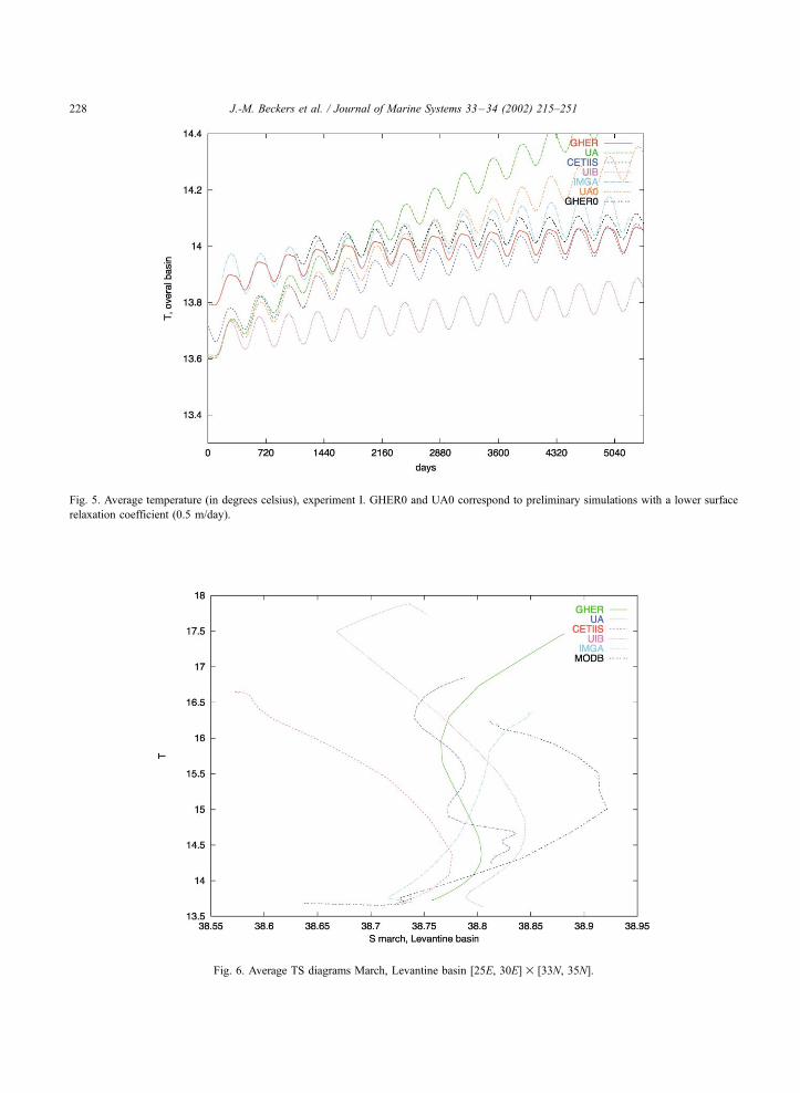
Fig. 5. Average temperature (in degrees celsius), experiment I. GHER0 and UA0 correspond to preliminary simulations with a lower surface

relaxation coefficient (0.5 m/day).

Fig. 6. Average TS diagrams March, Levantine basin [25E, 30E]� [33N, 35N].

J.-M. Beckers et al. / Journal of Marine Systems 33–34 (2002) 215–251228

(Beckers, 1999; Beckers and Deleersnijder, 1993),

attenuated by mode-splitting techniques (Killworth

et al., 1991). Rigid lid models, on the other hand,

can use larger time-steps, but the elliptic solver penal-

ises the model at high resolutions.

The treatment of topography in the models is

related both to the horizontal staggering techniques

used and the vertical coordinate system retained. In

the present case, either terrain-following coordinates

or z-level models are used. Terrain following coordi-

nates (among which classical r-coordinates) allow for

correct representation of topographic slopes even

without high vertical resolutions, but are hampered

by difficulties of representing strong stratifications in

the presence of strong topographic variations. For z-

coordinate models, the situation is somewhat the

inverse. Topographic treatment generally needs some

hand-tuning by the modellers, specially in straits, in

order to accommodate for the constraints imposed by

the numerical discretisations: B-grids need for exam-

ple more lateral points in a strait than C-grids.

Horizontal diffusion parameterisations in the mod-

els are very diverse, partly because lateral diffusion is

not only used as a physical parameterisation but also

as a numerical filter related to the advection schemes.

On the contrary, vertical diffusion parameterisations

are in principle designed to parameterise unresolved

mixing processes in the vertical. Parameterisations

there range from constant diffusion values to k� l

closure schemes, the latter taking into account strat-

ification effects and transport of turbulence.

Tables 1 and 2 show that the vertical and horizontal

diffusion parameterisations are very diverse, not only

from the functional parameterisation, but also from

the values chosen. It should however be noted that

some of the model implementations changed their

diffusion coefficients after a first comparison of the

results with the partners. Values shown here are those

retained for the results shown hereafter. Here it can be

mentioned that the models with constant vertical

diffusion coefficient performed several model runs

to calibrate the value of this coefficient, so as to have

a closer agreement with MODB data and the average

model response.

Models with turbulent closure schemes rather

modified the horizontal diffusion parameterisation

and coefficient values when carrying out new simu-

lations.

Here it is worth mentioning that the POM model

(UA) tried several ways to circumvent the classical

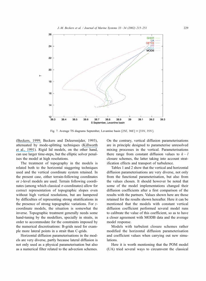
Fig. 7. Average TS diagrams September, Levantine basin [25E, 30E ]� [33N, 35N ].

J.-M. Beckers et al. / Journal of Marine Systems 33–34 (2002) 215–251 229

problem of r-coordinate models which diffuse on

numerical coordinate surfaces of constant r, whichcauses problems in regions where strong stratifica-

tions meet strong topographic gradients. Subtracting

mean vertical temperature and salinity profiles before

diffusing, reducing the Smagorinsky coefficients, etc.,

did not correct for a stronger drift in the subbasins

observed in the POM implementation compared to the

other models. Recently, the stronger drift was shown

to result indeed from the horizontal diffusion part, and

a modified rotated diffusion (Nittis and Lascaratos,

1999) has put the UA results more in line with the

other models subbasin drifts.

Figs. 1–4 represent horizontal distributions for

salinity and velocity fields during an averaged March

situation for the different models after the 15 years of

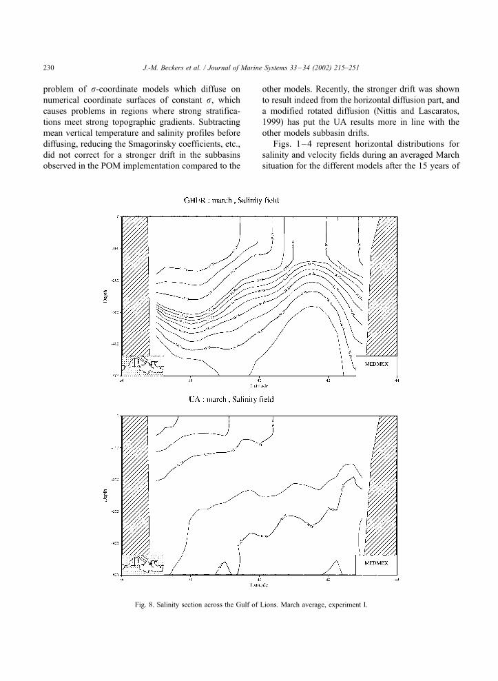
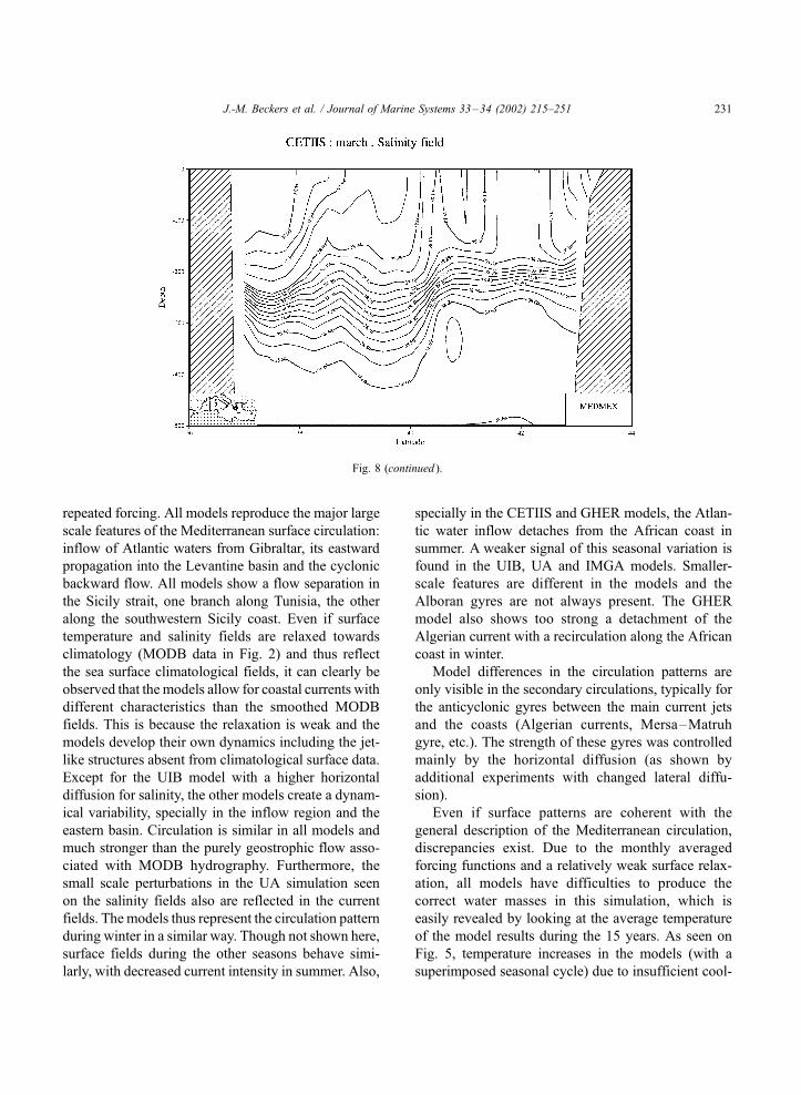
Fig. 8. Salinity section across the Gulf of Lions. March average, experiment I.

J.-M. Beckers et al. / Journal of Marine Systems 33–34 (2002) 215–251230

repeated forcing. All models reproduce the major large

scale features of the Mediterranean surface circulation:

inflow of Atlantic waters from Gibraltar, its eastward

propagation into the Levantine basin and the cyclonic

backward flow. All models show a flow separation in

the Sicily strait, one branch along Tunisia, the other

along the southwestern Sicily coast. Even if surface

temperature and salinity fields are relaxed towards

climatology (MODB data in Fig. 2) and thus reflect

the sea surface climatological fields, it can clearly be

observed that the models allow for coastal currents with

different characteristics than the smoothed MODB

fields. This is because the relaxation is weak and the

models develop their own dynamics including the jet-

like structures absent from climatological surface data.

Except for the UIB model with a higher horizontal

diffusion for salinity, the other models create a dynam-

ical variability, specially in the inflow region and the

eastern basin. Circulation is similar in all models and

much stronger than the purely geostrophic flow asso-

ciated with MODB hydrography. Furthermore, the

small scale perturbations in the UA simulation seen

on the salinity fields also are reflected in the current

fields. The models thus represent the circulation pattern

during winter in a similar way. Though not shown here,

surface fields during the other seasons behave simi-

larly, with decreased current intensity in summer. Also,

specially in the CETIIS and GHER models, the Atlan-

tic water inflow detaches from the African coast in

summer. A weaker signal of this seasonal variation is

found in the UIB, UA and IMGA models. Smaller-

scale features are different in the models and the

Alboran gyres are not always present. The GHER

model also shows too strong a detachment of the

Algerian current with a recirculation along the African

coast in winter.

Model differences in the circulation patterns are

only visible in the secondary circulations, typically for

the anticyclonic gyres between the main current jets

and the coasts (Algerian currents, Mersa–Matruh

gyre, etc.). The strength of these gyres was controlled

mainly by the horizontal diffusion (as shown by

additional experiments with changed lateral diffu-

sion).

Even if surface patterns are coherent with the

general description of the Mediterranean circulation,

discrepancies exist. Due to the monthly averaged

forcing functions and a relatively weak surface relax-

ation, all models have difficulties to produce the

correct water masses in this simulation, which is

easily revealed by looking at the average temperature

of the model results during the 15 years. As seen on

Fig. 5, temperature increases in the models (with a

superimposed seasonal cycle) due to insufficient cool-

Fig. 8 (continued ).

J.-M. Beckers et al. / Journal of Marine Systems 33–34 (2002) 215–251 231

ing and vertical mixing in winter. It is worth noting

that the models with constant vertical diffusion exhibit

the stronger drifts and that a change in the relaxation

coefficient (compare UA with UA0 and GHER with

GHER0) does lead to changes in the drifts, but these

changes are smaller than the differences in drifts

between the models. A temperature drift is observed

in all models, on which the annual cycle is super-

imposed. If we denote by T the annual average and by

hi the spatial average, we have the following relation-

ship describing the time-evolution of the mean tem-

perature in the basin:

qCpVdhTidt

¼ �ShQi ð2Þ

where V is the volume of the basin and S its surface.

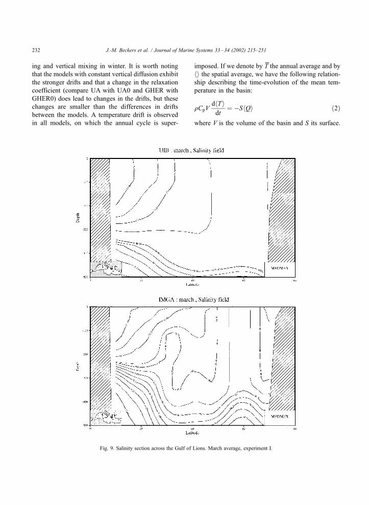
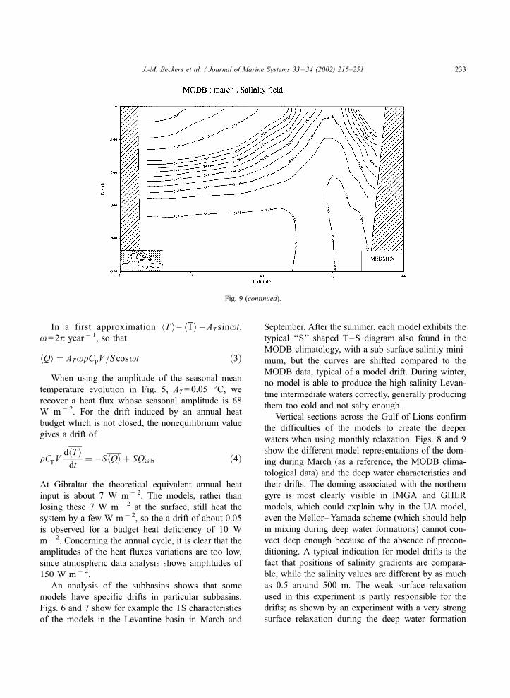
Fig. 9. Salinity section across the Gulf of Lions. March average, experiment I.

J.-M. Beckers et al. / Journal of Marine Systems 33–34 (2002) 215–251232

In a first approximation hT i= hTi�AT sinxt,

x = 2p year � 1, so that

hQi ¼ ATxqCpV=S cosxt ð3Þ

When using the amplitude of the seasonal mean

temperature evolution in Fig. 5, AT= 0.05 jC, we

recover a heat flux whose seasonal amplitude is 68

W m � 2. For the drift induced by an annual heat

budget which is not closed, the nonequilibrium value

gives a drift of

qCpVdhTidt

¼ �ShQi þ SQGib ð4Þ

At Gibraltar the theoretical equivalent annual heat

input is about 7 W m � 2. The models, rather than

losing these 7 W m� 2 at the surface, still heat the

system by a few W m � 2, so the a drift of about 0.05

is observed for a budget heat deficiency of 10 W

m � 2. Concerning the annual cycle, it is clear that the

amplitudes of the heat fluxes variations are too low,

since atmospheric data analysis shows amplitudes of

150 W m � 2.

An analysis of the subbasins shows that some

models have specific drifts in particular subbasins.

Figs. 6 and 7 show for example the TS characteristics

of the models in the Levantine basin in March and

September. After the summer, each model exhibits the

typical ‘‘S’’ shaped T–S diagram also found in the

MODB climatology, with a sub-surface salinity mini-

mum, but the curves are shifted compared to the

MODB data, typical of a model drift. During winter,

no model is able to produce the high salinity Levan-

tine intermediate waters correctly, generally producing

them too cold and not salty enough.

Vertical sections across the Gulf of Lions confirm

the difficulties of the models to create the deeper

waters when using monthly relaxation. Figs. 8 and 9

show the different model representations of the dom-

ing during March (as a reference, the MODB clima-

tological data) and the deep water characteristics and

their drifts. The doming associated with the northern

gyre is most clearly visible in IMGA and GHER

models, which could explain why in the UA model,

even the Mellor–Yamada scheme (which should help

in mixing during deep water formations) cannot con-

vect deep enough because of the absence of precon-

ditioning. A typical indication for model drifts is the

fact that positions of salinity gradients are compara-

ble, while the salinity values are different by as much

as 0.5 around 500 m. The weak surface relaxation

used in this experiment is partly responsible for the

drifts; as shown by an experiment with a very strong

surface relaxation during the deep water formation

Fig. 9 (continued).

J.-M. Beckers et al. / Journal of Marine Systems 33–34 (2002) 215–251 233

phases, it is possible to form the necessary deep

waters (Myers and Keith, 2000).

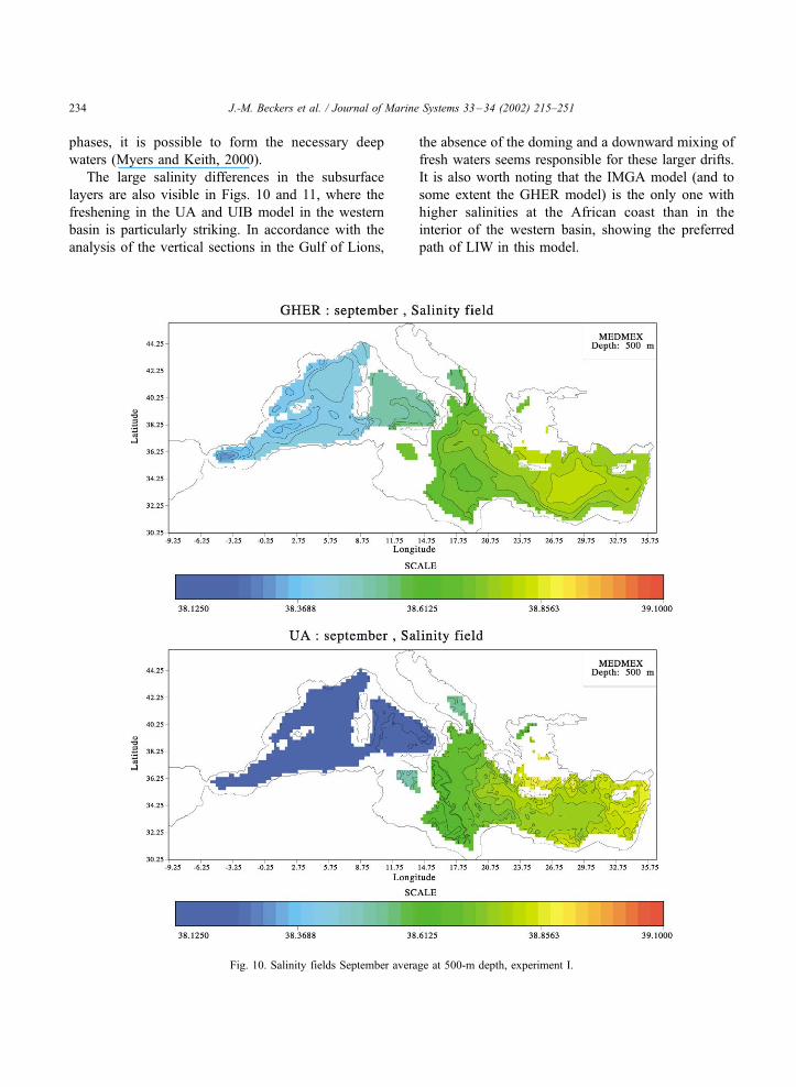
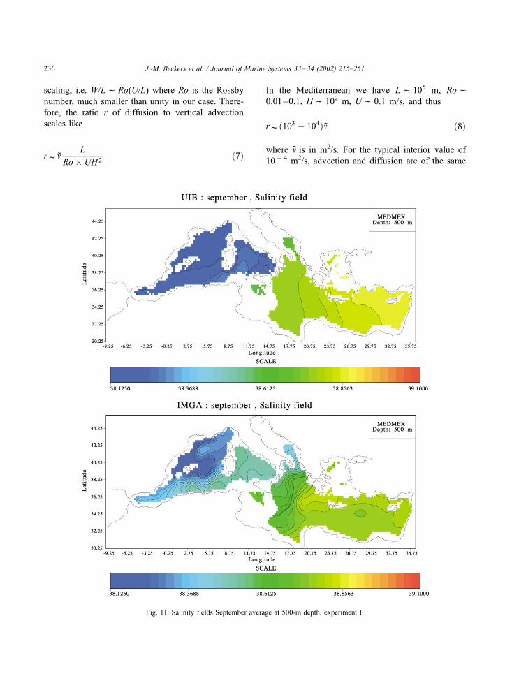
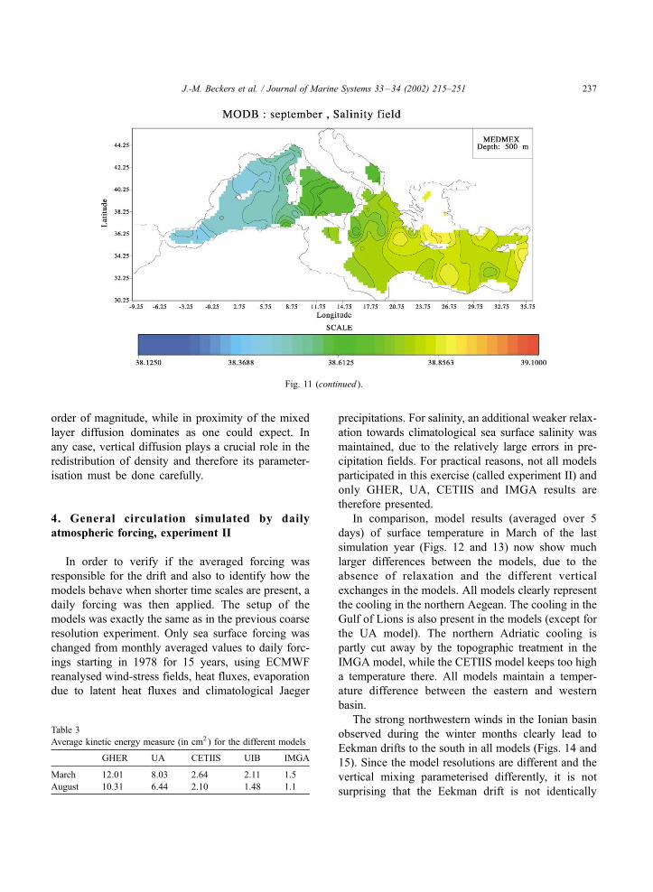
The large salinity differences in the subsurface

layers are also visible in Figs. 10 and 11, where the

freshening in the UA and UIB model in the western

basin is particularly striking. In accordance with the

analysis of the vertical sections in the Gulf of Lions,

the absence of the doming and a downward mixing of

fresh waters seems responsible for these larger drifts.

It is also worth noting that the IMGA model (and to

some extent the GHER model) is the only one with

higher salinities at the African coast than in the

interior of the western basin, showing the preferred

path of LIW in this model.

Fig. 10. Salinity fields September average at 500-m depth, experiment I.

J.-M. Beckers et al. / Journal of Marine Systems 33–34 (2002) 215–251234

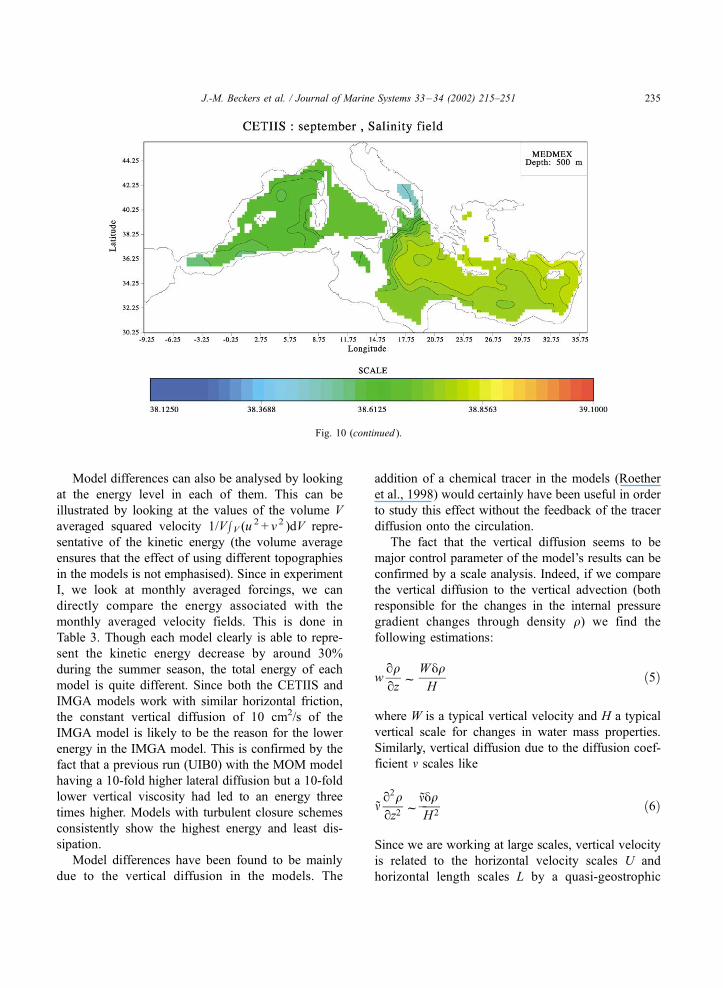
Model differences can also be analysed by looking

at the energy level in each of them. This can be

illustrated by looking at the values of the volume V

averaged squared velocity 1/VmV (u2 + v 2 )dV repre-

sentative of the kinetic energy (the volume average

ensures that the effect of using different topographies

in the models is not emphasised). Since in experiment

I, we look at monthly averaged forcings, we can

directly compare the energy associated with the

monthly averaged velocity fields. This is done in

Table 3. Though each model clearly is able to repre-

sent the kinetic energy decrease by around 30%

during the summer season, the total energy of each

model is quite different. Since both the CETIIS and

IMGA models work with similar horizontal friction,

the constant vertical diffusion of 10 cm2/s of the

IMGA model is likely to be the reason for the lower

energy in the IMGA model. This is confirmed by the

fact that a previous run (UIB0) with the MOM model

having a 10-fold higher lateral diffusion but a 10-fold

lower vertical viscosity had led to an energy three

times higher. Models with turbulent closure schemes

consistently show the highest energy and least dis-

sipation.

Model differences have been found to be mainly

due to the vertical diffusion in the models. The

addition of a chemical tracer in the models (Roether

et al., 1998) would certainly have been useful in order

to study this effect without the feedback of the tracer

diffusion onto the circulation.

The fact that the vertical diffusion seems to be

major control parameter of the model’s results can be

confirmed by a scale analysis. Indeed, if we compare

the vertical diffusion to the vertical advection (both

responsible for the changes in the internal pressure

gradient changes through density q) we find the

following estimations:

wqqqz

fWyqH

ð5Þ

where W is a typical vertical velocity and H a typical

vertical scale for changes in water mass properties.

Similarly, vertical diffusion due to the diffusion coef-

ficient m˜ scales like

mq2qqz2

fm�yqH2

ð6Þ

Since we are working at large scales, vertical velocity

is related to the horizontal velocity scales U and

horizontal length scales L by a quasi-geostrophic

Fig. 10 (continued ).

J.-M. Beckers et al. / Journal of Marine Systems 33–34 (2002) 215–251 235

scaling, i.e. W/LfRo(U/L) where Ro is the Rossby

number, much smaller than unity in our case. There-

fore, the ratio r of diffusion to vertical advection

scales like

rfmL

Ro� UH2ð7Þ

In the Mediterranean we have Lf 105 m, Rof0.01–0.1, Hf 102 m, Uf 0.1 m/s, and thus

rfð103 � 104Þm ð8Þ

where m is in m2/s. For the typical interior value of

10� 4 m2/s, advection and diffusion are of the same

Fig. 11. Salinity fields September average at 500-m depth, experiment I.

J.-M. Beckers et al. / Journal of Marine Systems 33–34 (2002) 215–251236

order of magnitude, while in proximity of the mixed

layer diffusion dominates as one could expect. In

any case, vertical diffusion plays a crucial role in the

redistribution of density and therefore its parameter-

isation must be done carefully.

4. General circulation simulated by daily

atmospheric forcing, experiment II

In order to verify if the averaged forcing was

responsible for the drift and also to identify how the

models behave when shorter time scales are present, a

daily forcing was then applied. The setup of the

models was exactly the same as in the previous coarse

resolution experiment. Only sea surface forcing was

changed from monthly averaged values to daily forc-

ings starting in 1978 for 15 years, using ECMWF

reanalysed wind-stress fields, heat fluxes, evaporation

due to latent heat fluxes and climatological Jaeger

precipitations. For salinity, an additional weaker relax-

ation towards climatological sea surface salinity was

maintained, due to the relatively large errors in pre-

cipitation fields. For practical reasons, not all models

participated in this exercise (called experiment II) and

only GHER, UA, CETIIS and IMGA results are

therefore presented.

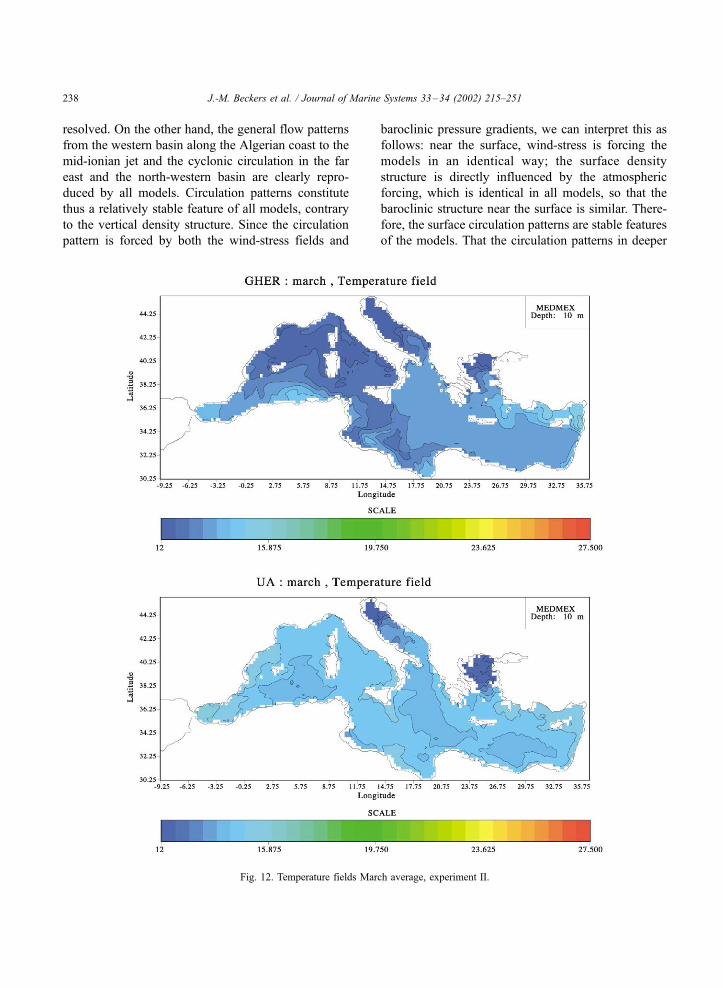
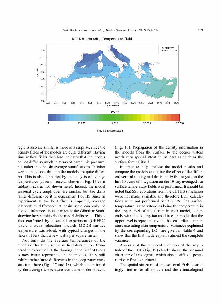
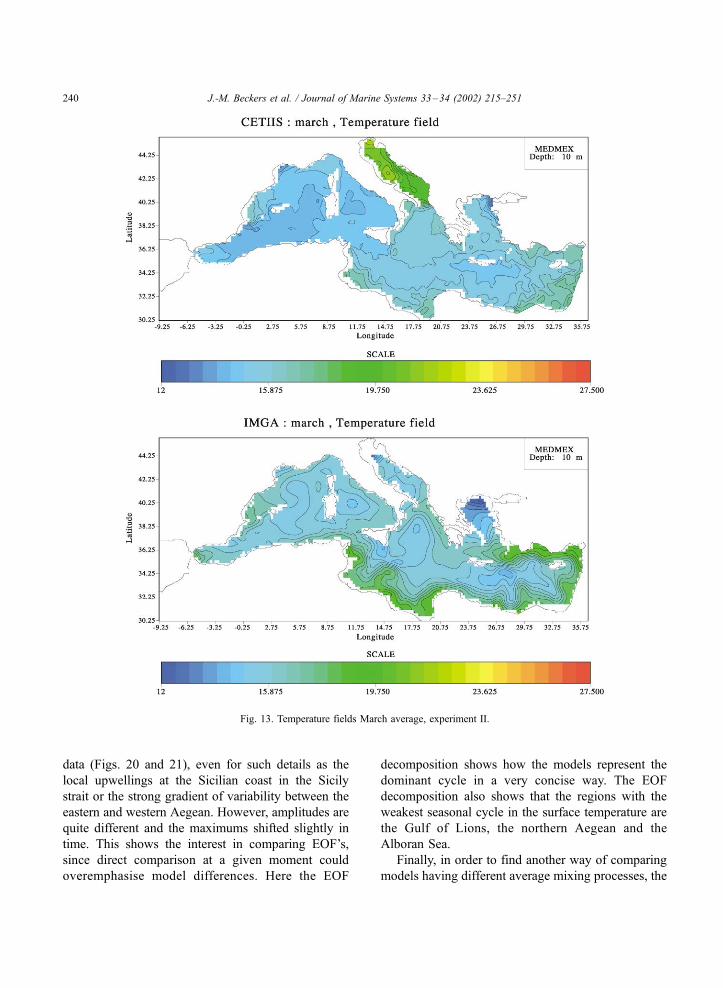
In comparison, model results (averaged over 5

days) of surface temperature in March of the last

simulation year (Figs. 12 and 13) now show much

larger differences between the models, due to the

absence of relaxation and the different vertical

exchanges in the models. All models clearly represent

the cooling in the northern Aegean. The cooling in the

Gulf of Lions is also present in the models (except for

the UA model). The northern Adriatic cooling is

partly cut away by the topographic treatment in the

IMGA model, while the CETIIS model keeps too high

a temperature there. All models maintain a temper-

ature difference between the eastern and western

basin.

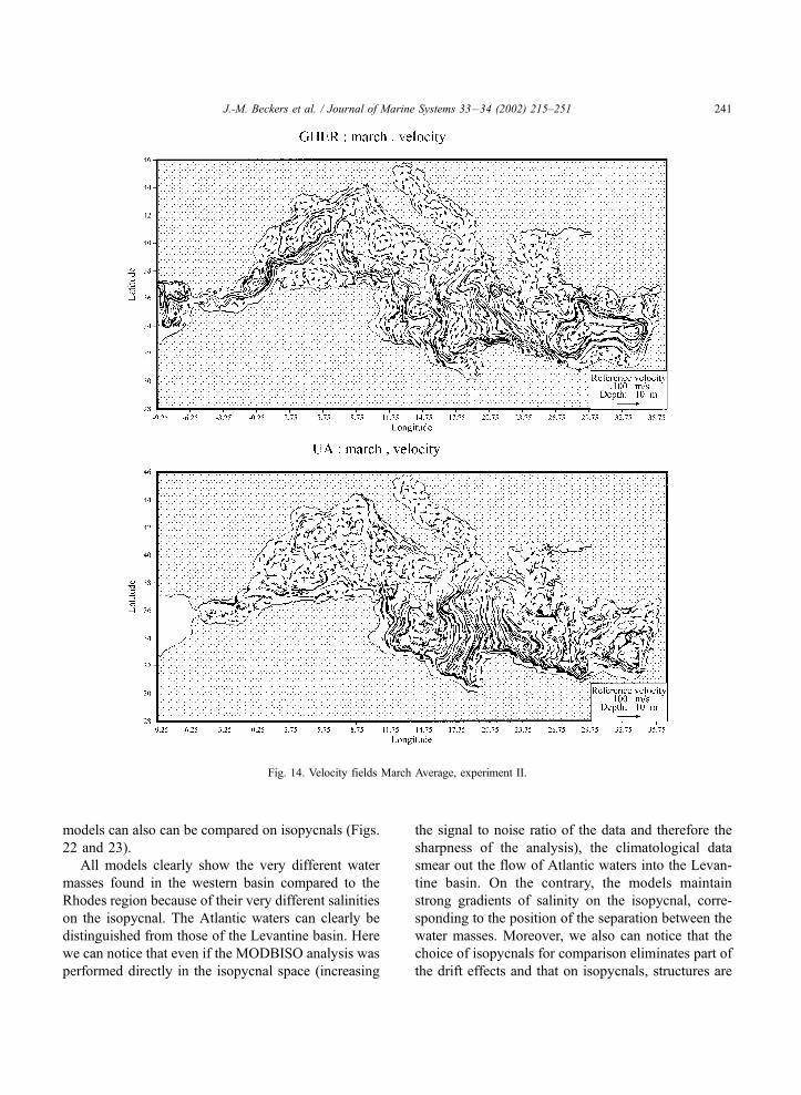
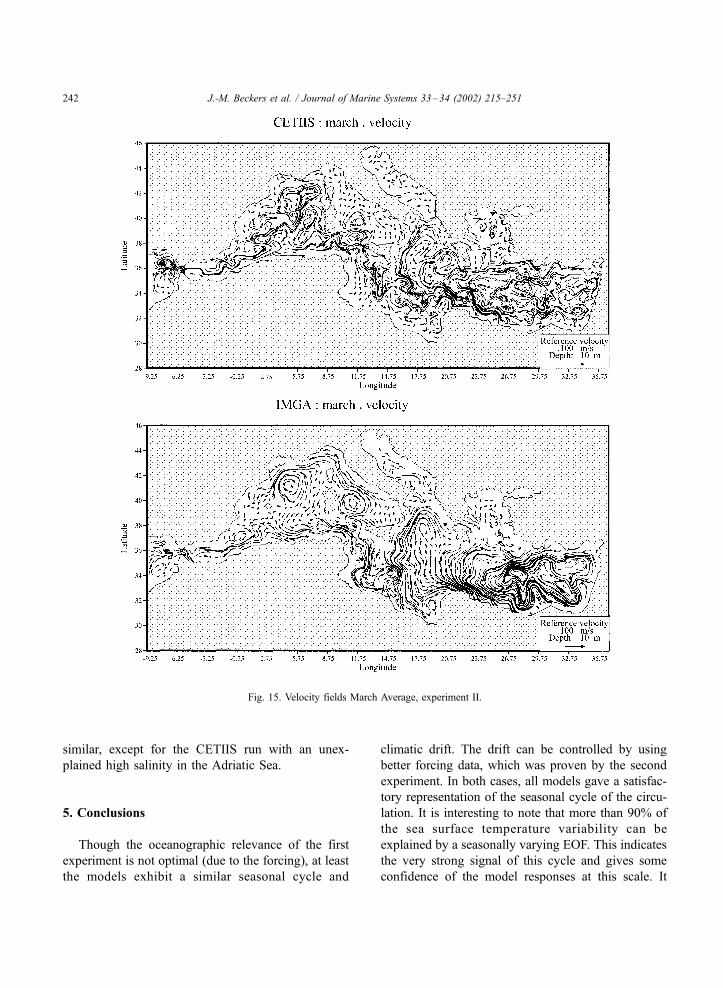
The strong northwestern winds in the Ionian basin

observed during the winter months clearly lead to

Eekman drifts to the south in all models (Figs. 14 and

15). Since the model resolutions are different and the

vertical mixing parameterised differently, it is not

surprising that the Eekman drift is not identically

Fig. 11 (continued ).

Table 3

Average kinetic energy measure (in cm2 ) for the different models

GHER UA CETIIS UIB IMGA

March 12.01 8.03 2.64 2.11 1.5

August 10.31 6.44 2.10 1.48 1.1

J.-M. Beckers et al. / Journal of Marine Systems 33–34 (2002) 215–251 237

resolved. On the other hand, the general flow patterns

from the western basin along the Algerian coast to the

mid-ionian jet and the cyclonic circulation in the far

east and the north-western basin are clearly repro-

duced by all models. Circulation patterns constitute

thus a relatively stable feature of all models, contrary

to the vertical density structure. Since the circulation

pattern is forced by both the wind-stress fields and

baroclinic pressure gradients, we can interpret this as

follows: near the surface, wind-stress is forcing the

models in an identical way; the surface density

structure is directly influenced by the atmospheric

forcing, which is identical in all models, so that the

baroclinic structure near the surface is similar. There-

fore, the surface circulation patterns are stable features

of the models. That the circulation patterns in deeper

Fig. 12. Temperature fields March average, experiment II.

J.-M. Beckers et al. / Journal of Marine Systems 33–34 (2002) 215–251238

regions also are similar is more of a surprise, since the

density fields of the models are quite different. Having

similar flow fields therefore indicates that the models

do not differ so much in terms of baroclinic pressure,

but rather in subbasin average stratifications. In other

words, the global drifts in the models are quite differ-

ent. This is also supported by the analysis of average

temperatures (at basin scale as shown in Fig. 16 or at

subbasin scales not shown here). Indeed, the model

seasonal cycle amplitudes are similar, but the drifts

rather different (be it in experiment I or II). Since in

experiment II the heat flux is imposed, average

temperature differences at basin scale can only be

due to differences in exchanges at the Gibraltar Strait,

showing how sensitively the model drifts react. This is

also confirmed by a second experiment (GHER2)

where a weak relaxation towards MODB surface

temperature was added, with typical changes in the

fluxes of less than a few watts per square meter.

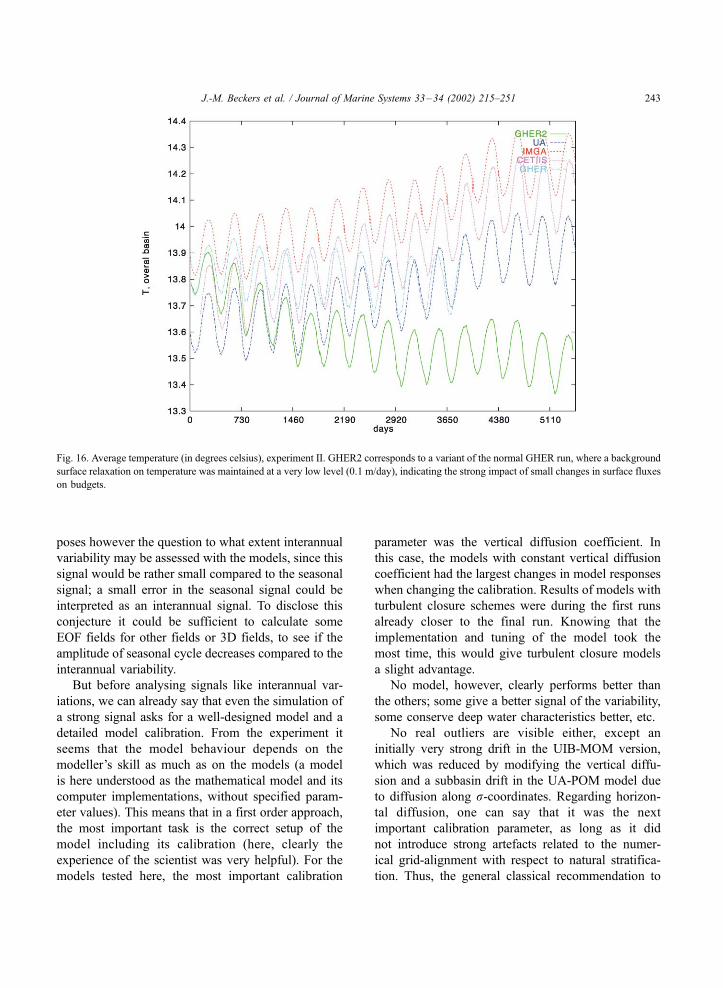
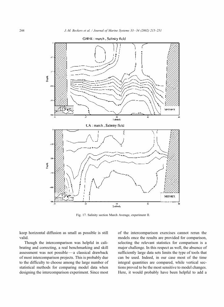
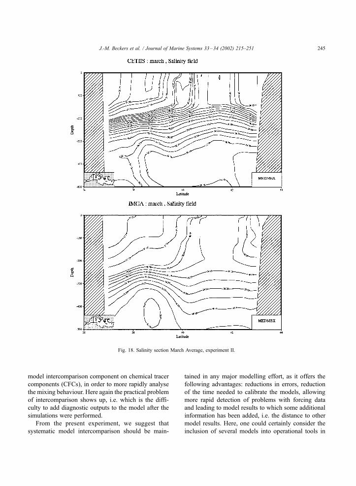
Not only do the average temperatures of the

models differ, but also the vertical distribution. Com-

pared to experiment I, the doming in the Gulf of Lions

is now better represented in the models. They still

exhibit rather large differences in the deep water mass

structure there (Figs. 17 and 18), which is confirmed

by the average temperature evolution in the models.

(Fig. 16). Propagation of the density information in

the models from the surface to the deeper waters

needs very special attention, at least as much as the

surface forcing itself.

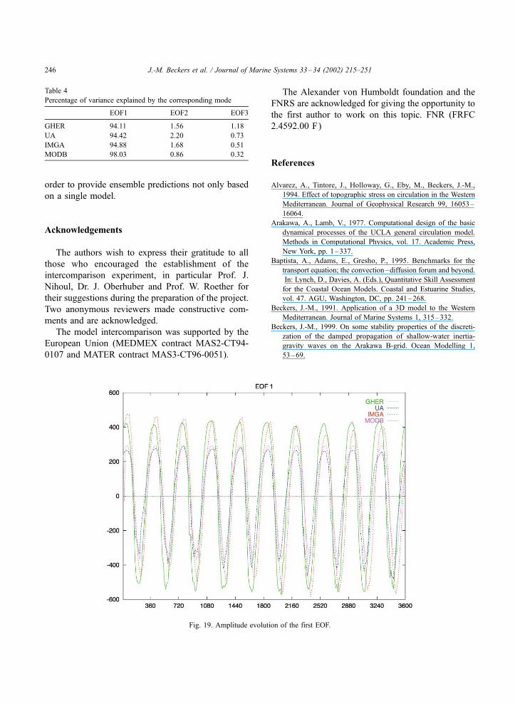
In order to help analyse the model results and

compare the models excluding the effect of the differ-

ent vertical mixing and drifts, an EOF analysis on the

last 10 years of integration on the 10-day averaged sea

surface temperature fields was performed. It should be

noted that SST evolutions from the CETIIS simulation

were not made available and therefore EOF calcula-

tions were not performed for CETIIS. Sea surface

temperature is understood as being the temperature in

the upper level of calculation in each model, coher-

ently with the assumption used in each model that the

upper level is representative of the sea surface temper-

ature excluding skin temperature. Variances explained

by the corresponding EOF are given in Table 4 and

show that the first mode explains almost the complete

variance.

Analysis of the temporal evolution of the ampli-

tude of the EOF (Fig. 19) clearly shows the seasonal

character of this signal, which also justifies a poste-

riori our first experiment.

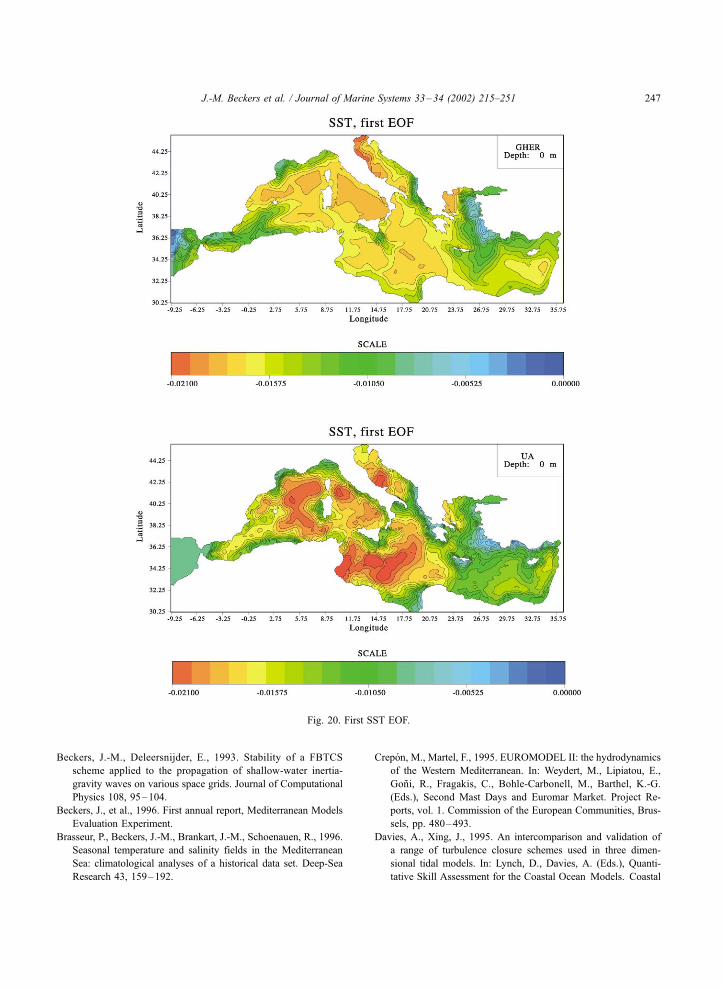
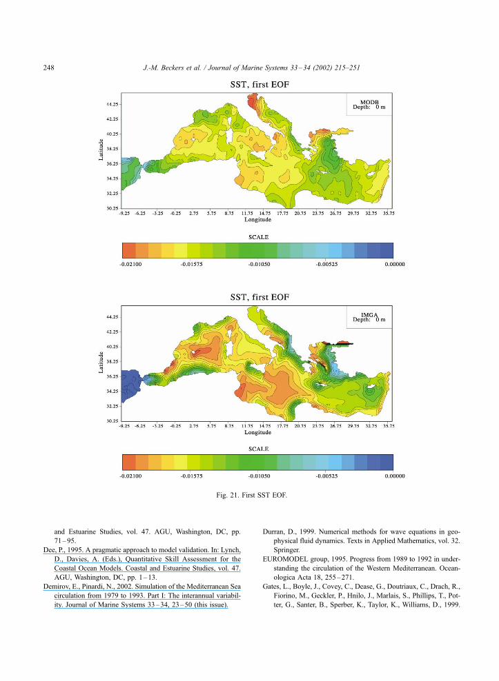
The spatial structure of this seasonal EOF is strik-

ingly similar for all models and the climatological

Fig. 12 (continued ).

J.-M. Beckers et al. / Journal of Marine Systems 33–34 (2002) 215–251 239

data (Figs. 20 and 21), even for such details as the

local upwellings at the Sicilian coast in the Sicily

strait or the strong gradient of variability between the

eastern and western Aegean. However, amplitudes are

quite different and the maximums shifted slightly in

time. This shows the interest in comparing EOF’s,

since direct comparison at a given moment could

overemphasise model differences. Here the EOF

decomposition shows how the models represent the

dominant cycle in a very concise way. The EOF

decomposition also shows that the regions with the

weakest seasonal cycle in the surface temperature are

the Gulf of Lions, the northern Aegean and the

Alboran Sea.

Finally, in order to find another way of comparing

models having different average mixing processes, the

Fig. 13. Temperature fields March average, experiment II.

J.-M. Beckers et al. / Journal of Marine Systems 33–34 (2002) 215–251240

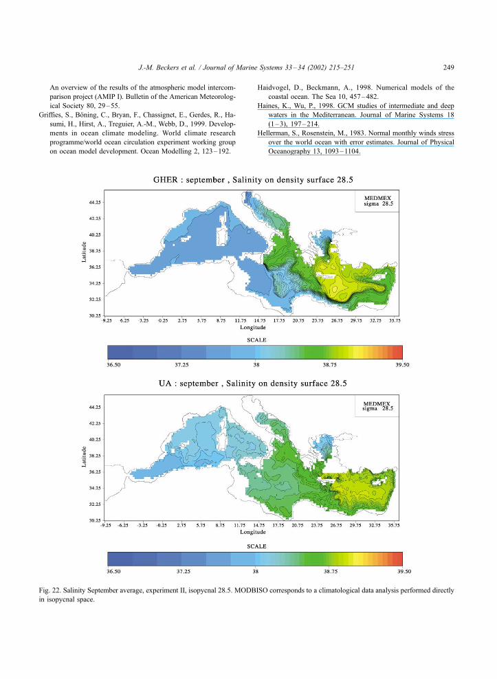
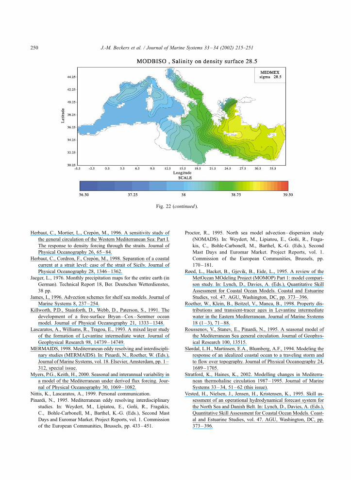
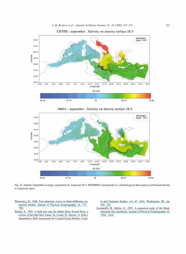
models can also can be compared on isopycnals (Figs.

22 and 23).

All models clearly show the very different water

masses found in the western basin compared to the

Rhodes region because of their very different salinities

on the isopycnal. The Atlantic waters can clearly be

distinguished from those of the Levantine basin. Here

we can notice that even if the MODBISO analysis was

performed directly in the isopycnal space (increasing

the signal to noise ratio of the data and therefore the

sharpness of the analysis), the climatological data

smear out the flow of Atlantic waters into the Levan-

tine basin. On the contrary, the models maintain

strong gradients of salinity on the isopycnal, corre-

sponding to the position of the separation between the

water masses. Moreover, we also can notice that the

choice of isopycnals for comparison eliminates part of

the drift effects and that on isopycnals, structures are

Fig. 14. Velocity fields March Average, experiment II.

J.-M. Beckers et al. / Journal of Marine Systems 33–34 (2002) 215–251 241

similar, except for the CETIIS run with an unex-

plained high salinity in the Adriatic Sea.

5. Conclusions

Though the oceanographic relevance of the first

experiment is not optimal (due to the forcing), at least

the models exhibit a similar seasonal cycle and

climatic drift. The drift can be controlled by using

better forcing data, which was proven by the second

experiment. In both cases, all models gave a satisfac-

tory representation of the seasonal cycle of the circu-

lation. It is interesting to note that more than 90% of

the sea surface temperature variability can be

explained by a seasonally varying EOF. This indicates

the very strong signal of this cycle and gives some

confidence of the model responses at this scale. It

Fig. 15. Velocity fields March Average, experiment II.

J.-M. Beckers et al. / Journal of Marine Systems 33–34 (2002) 215–251242

poses however the question to what extent interannual

variability may be assessed with the models, since this

signal would be rather small compared to the seasonal

signal; a small error in the seasonal signal could be

interpreted as an interannual signal. To disclose this

conjecture it could be sufficient to calculate some

EOF fields for other fields or 3D fields, to see if the

amplitude of seasonal cycle decreases compared to the

interannual variability.

But before analysing signals like interannual var-

iations, we can already say that even the simulation of

a strong signal asks for a well-designed model and a

detailed model calibration. From the experiment it

seems that the model behaviour depends on the

modeller’s skill as much as on the models (a model

is here understood as the mathematical model and its

computer implementations, without specified param-

eter values). This means that in a first order approach,

the most important task is the correct setup of the

model including its calibration (here, clearly the

experience of the scientist was very helpful). For the

models tested here, the most important calibration

parameter was the vertical diffusion coefficient. In

this case, the models with constant vertical diffusion

coefficient had the largest changes in model responses

when changing the calibration. Results of models with

turbulent closure schemes were during the first runs

already closer to the final run. Knowing that the

implementation and tuning of the model took the

most time, this would give turbulent closure models

a slight advantage.

No model, however, clearly performs better than

the others; some give a better signal of the variability,

some conserve deep water characteristics better, etc.

No real outliers are visible either, except an

initially very strong drift in the UIB-MOM version,

which was reduced by modifying the vertical diffu-

sion and a subbasin drift in the UA-POM model due

to diffusion along r-coordinates. Regarding horizon-

tal diffusion, one can say that it was the next

important calibration parameter, as long as it did

not introduce strong artefacts related to the numer-

ical grid-alignment with respect to natural stratifica-

tion. Thus, the general classical recommendation to

Fig. 16. Average temperature (in degrees celsius), experiment II. GHER2 corresponds to a variant of the normal GHER run, where a background

surface relaxation on temperature was maintained at a very low level (0.1 m/day), indicating the strong impact of small changes in surface fluxes

on budgets.

J.-M. Beckers et al. / Journal of Marine Systems 33–34 (2002) 215–251 243

keep horizontal diffusion as small as possible is still

valid.

Though the intercomparison was helpful in cali-

brating and correcting, a real benchmarking and skill

assessment was not possible—a classical drawback

of most intercomparison projects. This is probably due

to the difficulty to choose among the large number of

statistical methods for comparing model data when

designing the intercomparison experiment. Since most

of the intercomparison exercises cannot rerun the

models once the results are provided for comparison,

selecting the relevant statistics for comparison is a

major challenge. In this respect as well, the absence of

sufficiently large data sets limits the type of tools that

can be used. Indeed, in our case most of the time

integral quantities are compared, while vertical sec-

tions proved to be the most sensitive to model changes.

Here, it would probably have been helpful to add a

Fig. 17. Salinity section March Average, experiment II.

J.-M. Beckers et al. / Journal of Marine Systems 33–34 (2002) 215–251244

model intercomparison component on chemical tracer

components (CFCs), in order to more rapidly analyse

the mixing behaviour. Here again the practical problem

of intercomparison shows up, i.e. which is the diffi-

culty to add diagnostic outputs to the model after the

simulations were performed.

From the present experiment, we suggest that

systematic model intercomparison should be main-

tained in any major modelling effort, as it offers the

following advantages: reductions in errors, reduction

of the time needed to calibrate the models, allowing

more rapid detection of problems with forcing data

and leading to model results to which some additional

information has been added, i.e. the distance to other

model results. Here, one could certainly consider the

inclusion of several models into operational tools in

Fig. 18. Salinity section March Average, experiment II.

J.-M. Beckers et al. / Journal of Marine Systems 33–34 (2002) 215–251 245

order to provide ensemble predictions not only based

on a single model.

Acknowledgements

The authors wish to express their gratitude to all

those who encouraged the establishment of the

intercomparison experiment, in particular Prof. J.

Nihoul, Dr. J. Oberhuber and Prof. W. Roether for

their suggestions during the preparation of the project.

Two anonymous reviewers made constructive com-

ments and are acknowledged.

The model intercomparison was supported by the

European Union (MEDMEX contract MAS2-CT94-

0107 and MATER contract MAS3-CT96-0051).

The Alexander von Humboldt foundation and the

FNRS are acknowledged for giving the opportunity to

the first author to work on this topic. FNR (FRFC

2.4592.00 F)

References

Alvarez, A., Tintore, J., Holloway, G., Eby, M., Beckers, J.-M.,

1994. Effect of topographic stress on circulation in the Western

Mediterranean. Journal of Geophysical Research 99, 16053–

16064.

Arakawa, A., Lamb, V., 1977. Computational design of the basic

dynamical processes of the UCLA general circulation model.

Methods in Computational Physics, vol. 17. Academic Press,

New York, pp. 1–337.

Baptista, A., Adams, E., Gresho, P., 1995. Benchmarks for the

transport equation; the convection–diffusion forum and beyond.

In: Lynch, D., Davies, A. (Eds.), Quantitative Skill Assessment

for the Coastal Ocean Models. Coastal and Estuarine Studies,

vol. 47. AGU, Washington, DC, pp. 241–268.

Beckers, J.-M., 1991. Application of a 3D model to the Western

Mediterranean. Journal of Marine Systems 1, 315–332.

Beckers, J.-M., 1999. On some stability properties of the discreti-

zation of the damped propagation of shallow-water inertia-

gravity waves on the Arakawa B-grid. Ocean Modelling 1,

53–69.

Table 4

Percentage of variance explained by the corresponding mode

EOF1 EOF2 EOF3

GHER 94.11 1.56 1.18

UA 94.42 2.20 0.73

IMGA 94.88 1.68 0.51

MODB 98.03 0.86 0.32

Fig. 19. Amplitude evolution of the first EOF.

J.-M. Beckers et al. / Journal of Marine Systems 33–34 (2002) 215–251246

Beckers, J.-M., Deleersnijder, E., 1993. Stability of a FBTCS

scheme applied to the propagation of shallow-water inertia-

gravity waves on various space grids. Journal of Computational

Physics 108, 95–104.

Beckers, J., et al., 1996. First annual report, Mediterranean Models

Evaluation Experiment.

Brasseur, P., Beckers, J.-M., Brankart, J.-M., Schoenauen, R., 1996.

Seasonal temperature and salinity fields in the Mediterranean

Sea: climatological analyses of a historical data set. Deep-Sea

Research 43, 159–192.

Crepon, M., Martel, F., 1995. EUROMODEL II: the hydrodynamics

of the Western Mediterranean. In: Weydert, M., Lipiatou, E.,

Goni, R., Fragakis, C., Bohle-Carbonell, M., Barthel, K.-G.

(Eds.), Second Mast Days and Euromar Market. Project Re-

ports, vol. 1. Commission of the European Communities, Brus-

sels, pp. 480–493.

Davies, A., Xing, J., 1995. An intercomparison and validation of

a range of turbulence closure schemes used in three dimen-

sional tidal models. In: Lynch, D., Davies, A. (Eds.), Quanti-

tative Skill Assessment for the Coastal Ocean Models. Coastal

Fig. 20. First SST EOF.

J.-M. Beckers et al. / Journal of Marine Systems 33–34 (2002) 215–251 247

and Estuarine Studies, vol. 47. AGU, Washington, DC, pp.

71–95.

Dee, P., 1995. A pragmatic approach to model validation. In: Lynch,

D., Davies, A. (Eds.), Quantitative Skill Assessment for the

Coastal Ocean Models. Coastal and Estuarine Studies, vol. 47.

AGU, Washington, DC, pp. 1–13.

Demirov, E., Pinardi, N., 2002. Simulation of the Mediterranean Sea

circulation from 1979 to 1993. Part I: The interannual variabil-

ity. Journal of Marine Systems 33–34, 23–50 (this issue).

Durran, D., 1999. Numerical methods for wave equations in geo-

physical fluid dynamics. Texts in Applied Mathematics, vol. 32.

Springer.

EUROMODEL group, 1995. Progress from 1989 to 1992 in under-

standing the circulation of the Western Mediterranean. Ocean-

ologica Acta 18, 255–271.

Gates, L., Boyle, J., Covey, C., Dease, G., Doutriaux, C., Drach, R.,

Fiorino, M., Geckler, P., Hnilo, J., Marlais, S., Phillips, T., Pot-

ter, G., Santer, B., Sperber, K., Taylor, K., Williams, D., 1999.

Fig. 21. First SST EOF.

J.-M. Beckers et al. / Journal of Marine Systems 33–34 (2002) 215–251248

An overview of the results of the atmospheric model intercom-

parison project (AMIP I). Bulletin of the American Meteorolog-

ical Society 80, 29–55.

Griffies, S., Boning, C., Bryan, F., Chassignet, E., Gerdes, R., Ha-

sumi, H., Hirst, A., Treguier, A.-M., Webb, D., 1999. Develop-

ments in ocean climate modeling. World climate research

programme/world ocean circulation experiment working group

on ocean model development. Ocean Modelling 2, 123–192.

Haidvogel, D., Beckmann, A., 1998. Numerical models of the

coastal ocean. The Sea 10, 457–482.

Haines, K., Wu, P., 1998. GCM studies of intermediate and deep

waters in the Mediterranean. Journal of Marine Systems 18

(1–3), 197–214.

Hellerman, S., Rosenstein, M., 1983. Normal monthly winds stress

over the world ocean with error estimates. Journal of Physical

Oceanography 13, 1093–1104.

Fig. 22. Salinity September average, experiment II, isopycnal 28.5. MODBISO corresponds to a climatological data analysis performed directly

in isopycnal space.

J.-M. Beckers et al. / Journal of Marine Systems 33–34 (2002) 215–251 249

Herbaut, C., Mortier, L., Crepon, M., 1996. A sensitivity study of

the general circulation of the Western Mediterranean Sea: Part I.

The response to density forcing through the straits. Journal of

Physical Oceanography 26, 65–84.

Herbaut, C., Cordron, F., Crepon, M., 1998. Separation of a coastal

current at a strait level: case of the strait of Sicily. Journal of

Physical Oceanography 28, 1346–1362.

Jaeger, L., 1976. Monthly precipitation maps for the entire earth (in

German). Technical Report 18, Ber. Deutschen Wetterdienstes,

38 pp.

James, I., 1996. Advection schemes for shelf sea models. Journal of

Marine Systems 8, 237–254.

Killworth, P.D., Stainforth, D., Webb, D., Paterson, S., 1991. The

development of a free-surface Bryan–Cox–Semtner ocean

model. Journal of Physical Oceanography 21, 1333–1348.

Lascaratos, A., Williams, R., Tragou, E., 1993. A mixed layer study

of the formation of Levantine intermediate water. Journal of

Geophysical Research 98, 14739–14749.

MERMAIDS, 1998. Mediterranean eddy resolving and interdiscipli-

nary studies (MERMAIDS). In: Pinardi, N., Roether, W. (Eds.),

Journal of Marine Systems, vol. 18. Elsevier, Amsterdam, pp. 1–

312, special issue.

Myers, P.G., Keith, H., 2000. Seasonal and interannual variability in

a model of the Mediterranean under derived flux forcing. Jour-

nal of Physical Oceanography 30, 1069–1082.

Nittis, K., Lascaratos, A., 1999. Personal communication.

Pinardi, N., 1995. Mediterranean eddy resolving interdisciplinary

studies. In: Weydert, M., Lipiatou, E., Goni, R., Fragakis,

C., Bohle-Carbonell, M., Barthel, K.-G. (Eds.), Second Mast

Days and Euromar Market. Project Reports, vol. 1. Commission

of the European Communities, Brussels, pp. 433–451.

Proctor, R., 1995. North sea model advection–dispersion study

(NOMADS). In: Weydert, M., Lipiatou, E., Goni, R., Fraga-

kis, C., Bohle-Carbonell, M., Barthel, K.-G. (Eds.), Second

Mast Days and Euromar Market. Project Reports, vol. 1.

Commission of the European Communities, Brussels, pp.

170–181.

Røed, L., Hacket, B., Gjevik, B., Eide, L., 1995. A review of the

MetOcean MOdeling Project (MOMOP) Part 1: model compari-

son study. In: Lynch, D., Davies, A. (Eds.), Quantitative Skill

Assessment for Coastal Ocean Models. Coastal and Estuarine

Studies, vol. 47. AGU, Washington, DC, pp. 373–396.

Roether, W., Klein, B., Beitzel, V., Manca, B., 1998. Property dis-

tributions and transient-tracer ages in Levantine intermediate

water in the Eastern Mediterranean. Journal of Marine Systems

18 (1–3), 71–88.

Roussenov, V., Stanev, E., Pinardi, N., 1995. A seasonal model of

the Mediterranean Sea general circulation. Journal of Geophys-

ical Research 100, 13515.

Slørdal, L.H., Martinsen, E.A., Blumberg, A.F., 1994. Modeling the

response of an idealized coastal ocean to a traveling storm and

to flow over topography. Journal of Physical Oceanography 24,

1689–1705.

Stratford, K., Haines, K., 2002. Modelling changes in Mediterra-

nean thermohaline circulation 1987–1995. Journal of Marine

Systems 33–34, 51–62 (this issue).

Vested, H., Nielsen, J., Jensen, H., Kristensen, K., 1995. Skill as-

sessment of an operational hydrodynamical forecast system for

the North Sea and Danish Belt. In: Lynch, D., Davies, A. (Eds.),

Quantitative Skill Assessment for Coastal Ocean Models. Coast-

al and Estuarine Studies, vol. 47. AGU, Washington, DC, pp.

373–396.

Fig. 22 (continued ).

J.-M. Beckers et al. / Journal of Marine Systems 33–34 (2002) 215–251250

Wajsowicz, R., 1986. Free planetary waves in finite-difference nu-

merical models. Journal of Physical Oceanography 16, 773–

789.

Werner, F., 1995. A field test case for tidally flows forced flows: a

review of the tidal flow forum. In: Lynch, D., Davies, A. (Eds.),

Quantitative Skill Assessment for Coastal Ocean Models. Coast-

al and Estuarine Studies, vol. 47. AGU, Washington, DC, pp.

269–283.

Zavatarelli, M., Mellor, G., 1995. A numerical study of the Medi-

terranean Sea circulation. Journal of Physical Oceanography 25,

1384–1414.

Fig. 23. Salinity September average, experiment II, isopycnal 28.5. MODBISO corresponds to a climatological data analysis performed directly

in isopycnal space.

J.-M. Beckers et al. / Journal of Marine Systems 33–34 (2002) 215–251 251