Integrated Computer-Aided Engineering 24 (2017) 171–185 ...

Integrated Computer-Aided Engineering 24 (2017) 171–185 171DOI 10.3233/ICA-170538IOS Press

Layer multiplexing FPGA implementation fordeep back-propagation learning

Francisco Ortega-Zamoranoa,b,∗, José M. Jereza, Iván Gómeza and Leonardo FrancoaaDepartment of Computer Languages and Computer Science, University of Málaga, Málaga, SpainbSchool of Mathematics and Computer Science, University of Yachay Tech, San Miguel de Urcuquí, Ecuador

Abstract. Training of large scale neural networks, like those used nowadays in Deep Learning schemes, requires long com-putational times or the use of high performance computation solutions like those based on cluster computation, GPU boards,etc. As a possible alternative, in this work the Back-Propagation learning algorithm is implemented in an FPGA board usinga multiplexing layer scheme, in which a single layer of neurons is physically implemented in parallel but can be reused anynumber of times in order to simulate multi-layer architectures. An on-chip implementation of the algorithm is carried out using atraining/validation scheme in order to avoid overfitting effects. The hardware implementation is tested on several configurations,permitting to simulate architectures comprising up to 127 hidden layers with a maximum number of neurons in each layer of 60neurons. We confirmed the correct implementation of the algorithm and compared the computational times against C and Matlabcode executed in a multicore supercomputer, observing a clear advantage of the proposed FPGA scheme. The layer multiplex-ing scheme used provides a simple and flexible approach in comparison to standard implementations of the Back-Propagationalgorithm representing an important step towards the FPGA implementation of deep neural networks, one of the most novel andsuccessful existing models for prediction problems.

Keywords: Hardware implementation, FPGA, supervised learning, deep neural networks, layer multiplexing

1. Introduction

Artificial Neural Networks (ANN) [12] are mathe-matical models inspired in the functioning of the brainthat have been successfully applied to clustering andclassification problems in several domains. The Back-Propagation algorithm (BP) introduced by Werbos in1974 [46] and popularized through the work of Rumel-hart et al. [38] is the most used learning procedure fortraining feed-forward neural networks (FFNN) archi-tectures for its application to classification and regres-sion problems. It is a gradient descent based methodthat minimizes the error between targets and networkoutputs, computing the derivatives of the error in anefficient way [25,36]. As a gradient descent algorithm

∗Corresponding author: Francisco Ortega-Zamorano, Departa-mento de Lenguajes y Ciencias de la Computación, Universidad deMálaga, Campus de Teatinos S/N, 29071, Málaga, Spain. E-mail:[email protected].

the search for a solution can get stuck in local minimabut in practice the algorithm is quite efficient, and assuch it has been applied to a wide range of areas likepattern recognition [23], medical diagnosis [37], stockmarket prediction [35], etc.

Even if with the actual computational power it ispossible to train neural networks models relatively fast,using large architectures and/or large patterns data setsmay require the use of parallel strategies to speed upthe training process. In particular, a recent popular-ized model known as Deep Learning and usually ap-plied to large training data sets, relies in a trainingprocess that may take several days or even weeks tobe completed [5,17]. In this sense alternatives basedon cluster computing, GPUs and FPGAs are sensiblestrategies, each of them having their benefits and draw-backs [10,29,43,44]. In particular, Field ProgrammableGate Arrays (FPGA) [18] are reprogrammable siliconchips, using prebuilt logic blocks and programmablerouting resources that can be configured to implement

ISSN 1069-2509/17/$35.00 c© 2017 – IOS Press and the author(s). All rights reserved

172 F. Ortega-Zamorano et al. / Layer multiplexing FPGA implementation for deep back-propagation learning

custom hardware functionality. Neuro-inspired mod-els of computations have a very large degree of par-allel processing of the information, and as such onethe main advantages of FPGA over previously men-tioned alternatives (cluster computing and GPUs) forimplementing them is the fact of their intrinsic paral-lelism. On the other hand, programming FPGA is rel-atively more complex than the other models, and thisfact might explain that they have not been much uti-lized yet for Deep Learning.

Several studies have analyzed the implementationof neural networks models in FPGAs [19–21,24,32],applying one of the two existing alternatives for theirimplementation: off and on chip. In off-chip learn-ing implementations [13,30] the training of the neu-ral network model is performed externally usually ina personal computer (PC) to which the FPGA is at-tached, and only the synaptic weights are transmittedto the FPGA that acts as a hardware accelerator. Onthe other hand on-chip learning implementations in-cludes both training and execution phases of the algo-rithm [6,32,41] permitting the whole process to be car-ried out in the FPGA board independently of an ex-ternal device. Existing specific implementations of theartificial neural network Back-Propagation algorithmin FPGA boards include the works of [9,29,31,39].In all of these works, the neural network architectureis previously prefixed by the designer, as the numberof neurons and hidden layers is limited by the FPGAresources available. Although recent advances on thecomputational power of these boards have permitted anincrease in the size of the architectures, the number oflayers that can be implemented is still limited, and assaid above also this number should be prefixed beforeits application.

For the previously mentioned reason, in this work alayer multiplexing scheme for the on-chip implemen-tation of BP algorithm in a VIRTEX-5 XC5VLX110TFPGA board is introduced. This scheme consists in im-plementing physically a single layer of neurons thatcan be reused any number of times in order to simulatearchitectures with any number of hidden layers [13].The number of hidden layers that can be used in a neu-ral architecture is only limited by the temporal con-straint related to the execution time and to a maxi-mum of 127 because of the memory resource design,although it has been observed previously [3,8] and con-firmed in the present work that the performance of theBP algorithm is drastically reduced when the numberof layers is too large. In this respect, a new promis-ing field named Deep Learning has attracted the at-

tention of several researchers and companies in re-cent years, due to the great success of deep neuralnetworks architectures in several pattern recognitioncontests [14,22,40]. Deep learning schemes requiresthe use of additional strategies or modifications to thestandard BP algorithm in order to be applied success-fully [45], but so far all existing alternative requiresheavy computational resources. The aim of this workis to build a simple and flexible implementation of theBP algorithm that may permit to simulate deep Back-Propagation neural networks efficiently, contributingto their study and application, and also opening newstrategies towards the simulation of deep learning neu-ral networks.

The organization of the present work is as follows:next section includes relevant implementation detailsabout the BP algorithm. The FPGA implementation isdescribed in Section 3, that contains the technical de-tails of the implementation. The work continues witha result section where the implementation is testedand characterized, and finishes with the discussion andconclusions.

2. The Back-Propagation algorithm

The Back-Propagation algorithm is a supervisedlearning method for training multilayer artificial neu-ral networks, and even if the algorithm is very wellknown, we summarize in this section the main equa-tions in relationship to the implementation of the Back-Propagation algorithm, as they are important in orderto understand the current work.

Let’s consider a neural network architecture com-prising several hidden layers. If we consider the neu-rons belonging to a hidden or output layer, the activa-tion of these units, denoted by yi, can be written as:

yi = g

⎛⎝

L∑j=1

wij · sj⎞⎠ = g(h), (1)

where wij are the synaptic weights between neuron iin the current layer and the neurons of the previouslayer with activation sj . In the previous equation, wehave introduced h as the synaptic potential of a neuron.The activation function used, g, is the logistic functiongiven by the following equation:

g(x) =1

1 + e−βx. (2)

The objective of the BP supervised learning algorithmis to minimize the difference between given outputs

F. Ortega-Zamorano et al. / Layer multiplexing FPGA implementation for deep back-propagation learning 173

(targets) for a set of input data and the output of thenetwork. This error depends on the values of the synap-tic weights, and so these should be adjusted in order tominimize the error. The error function computed for alloutput neurons can be defined as:

E =1

2

p∑k=1

M∑i=1

(zi(k)− yi(k))2, (3)

where the first sum is on the p patterns of the data setand the second sum is on the M output neurons. zi(k)is the target value for output neuron i for pattern k, andyi(k) is the corresponding response output of the net-work. By using the method of gradient descent, the BPattempts to minimize this error in an iterative processby updating the synaptic weights upon the presentationof a given pattern. The synaptic weights between twolast layers of neurons are updated as:

Δwij(k) = −η∂E

∂wij(k)

= η[zi(k)− yi(k)]g′i(hi)sj(k), (4)

where η is the learning rate that has to be set in ad-vance (a parameter of the algorithm), g′ is the deriva-tive of the sigmoid function and h is the synaptic po-tential previously defined, while the rest of the weightsare modified according to similar equations by the in-troduction of a set of values called the “deltas” (δ), thatpropagate the error from the last layer into the innerones, that are computed according to Eqs (5) and (6).

The delta values for the neurons of the last of the Nhidden layers are computed as:

δNj = (SNj )′[zj − SN

j ] (5)

The delta values for the rest of the hidden layer neu-rons are computed according to:

δlj = (Slj)

′ ∑wijδl+1i . (6)

Training and validation processesThe training procedure is executed a certain number

of times (epochs) using the training patterns. In oneepoch, all training patterns are presented once in ran-dom ordering, adjusting the synaptic weights in an on-line manner. A well known and severe problem affect-ing all predictive algorithms is the problem of overfit-ting, caused by an overspecialization of the learningprocedure on the training set of patterns [11]. In orderto alleviate this effect, one straightforward alternative

is to split the set of available training patterns in train-ing, validation and test sets. From these sets by the ap-plication of Eq. (3) training, validation and generaliza-tion error measures are obtained, measures that will bedenoted as Etr, Eval and Egen respectively. The train-ing set will then be used to adjust the synaptic weightsaccording to Eq. (4), while the validation set is used tocontrol overfitting effects, storing in memory the val-ues of the synaptic weights that have so far led to thelowest validation error, so when the training procedureends, the algorithm returns the stored set of weights.The test set is used to estimate the performance of thealgorithm in unseen data patterns. The generalizationability (Gen) defined as Gen = 1 − Egen is a stan-dard measure for the prediction accuracy of an algo-rithm, obtaining its optimal value for Gen = 1 whenEgen = 0.

3. FPGA layer multiplexing schemeimplementation of the BP algorithm

The hardware implementation of the Back-Propaga-tion algorithm is divided in 3 different processes: thecomputation of the output of the neurons (S values),the calculation of the deltas of each neuron (δ), and thesynaptic weight updating procedure. Given the logic ofthe Back-Propagation algorithm, in which the S val-ues are obtained in a forward manner (from the in-put towards the output) while the deltas are computedbackwards, and that finally the weights updating is ex-ecuted with the values previously obtained, the threeprocesses are sequentially implemented. It is possibleto perform the weight updating phase at the same timethat the deltas are computed but we have preferred toseparate all three processes to obtain a clearer design.

The S values of every layer are obtained as a func-tion of the S values of the previous layer neurons ex-cept for those from the first hidden layer which pro-cesses the information of the current input pattern. Onthe contrary, the δ values are computed backwardly,i.e., the δ values associated to a neuron belonging to ahidden layer are computed as a function of the δ valuesof the a deeper hidden layer, except for the last hiddenlayer which computes its δ values as a function of theerror committed on the current input pattern (cf. Eqs 5–6). The updating process is carried out with the S andδ values of every layer, so it is necessary to store thesevalues when they are computed to be used for the sys-tem when they are required. Thus, the structure of theBack-Propagation algorithm allows the whole process


Layer1

Inputs

Outp uts

Layer2

LayerN

(a) Standard Feed-forward neural network

Multi plexingLaye r

Inputs

Ou tputsYes

No

IfCurrentLayer

=MaxLayer ?

(b) Layer multiplexing scheme

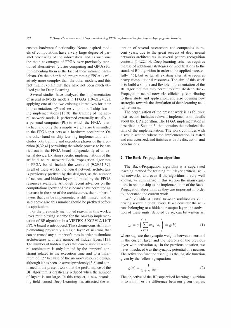
Fig. 1. (a) Standard feed-forward neural network architecture. (b)Layer multiplexing scheme for the simulation of deep feed-forwardneural network architectures.

to be implemented using a layer multiplexing schemebut noting that forward and backward phases shouldbe considered separately, as S and δ values cannot becomputed in a single forward phase.

The deep design of the Back-Propagation algorithmis based on a layer multiplexing scheme in whichonly one layer is physically implemented being reused3 × N times in order to simulate a whole neural net-work architecture containing N hidden layers. Fig-ure 1(a) shows the standard design of a feed-forwardneural network architecture where it can be observedhow the flow of information goes from the input to-wards the output, in a way that the input of a layer ofneurons is the output of the previous layer. In a layermultiplexing scheme, as shown in Fig. 1(b) the samewhole process is carried out but by reusing the struc-ture of the single implemented layer.

The implementation of the layer multiplexingscheme requires a precise control of which layer is sim-ulated in every moment, and for this reason a regis-ter called “CurrentLayer” is used. For each pattern, theprocess starts with the forward phase in which the out-put of the neurons are computed in response to the in-put pattern. This first phase starts by introducing an in-put pattern in the single multiplexing layer and by set-

ting the variable “CurrentLayer” set to 1. Then the neu-rons’ outputs are computed, stored in the distributedRAM memory and transmitted back to the input to cal-culate the following layer outputs, and thus the vari-able “CurrentLayer” is increased. The same process isrepeated sequentially until the “CurrentLayer” value isequal to the maximum number of layers, previously de-fined by the user and stored in the “MaxLayer” regis-ter. When the last layer is reached the neurons output iscomputed together with the error committed in the pat-tern target estimation and these error values are storedin a register for its use in the second phase. The sec-ond phase involves the backward computation of thedelta values, and the first computation involves the cal-culation of the delta values of the last layer. Once thesevalues are obtained, they are backwardly transmittedto the previous layer in order to compute the delta val-ues for these set of neurons, according to Eq. (6). Withthese delta values a recurrent process is used to obtainthe delta values of the rest of the layers until the in-put layer values are obtained (“CurrentLayer = 1”).At this point the third phase is carried out in order toupdate the synaptic weights, and finishing one patterniteration of the process.

In the following subsections details of the hardwareimplementation are given.

Hardware implementation design

Figure 2 shows the general structure of the hard-ware implementation of the Back-Propagation algo-rithm. The whole structure has been divided in twomain modules in order to separate the communicationprotocol and the memory resources of the FPGA (ex-ternal block) from the module where the implementa-tion of the algorithm is carried out composed by theArchitecture and Control blocks.

The External block logic depends specifically onthe type of communication protocol chosen for receiv-ing the pattern data set and transmitting the synapticweights of the resultant model. The implementationof the present algorithm in different applications andboards require the use of a different external block, soinstead of giving specific details about it, we have pre-ferred to describe its functionality that it might be morehelpful for future implementations.

In our case, the communication between the PC andthe FPGA was handled using a serial communicationprotocol through the RS-232 port of the board in orderto manage the exchange of information. The reason forthis choice is that it can be implemented in VHDL and


Pattern

New_Pattern

Ready_PatternsNew_ValidNew_TrainV_T

Enable_SentEnable_Store

EndReady_SentReady_Store

Ready_Valid

Weigths

Clk_AClk_B Reset

ControlBlock

ArchitectureBlockExternal

Block

Ready_Train

Pattern

Data Conf. Set

Pattern

Weigths

Weigths

Specificprotocol logic

Ctrl setError

Fig. 2. Information flow exchange between the external module incharge of the communication protocols and memory resources man-agement, and the module composed by the control and architectureblocks.

ported to other architectures quite easily in comparisonto other possibilities.

The functionality of the external block is separatedin two different processes: The first one was in chargeof storing and managing the input training data set inorder to present a different pattern every time that thecontrol block requires it; while the second process wasused for storing the synaptic weights once the learn-ing process finishes (see Fig. 2). The hardware imple-mentation of these two processes involves taking intoaccount a series of signals between the blocks that aredescribed in the appendix.

The internal module computes the neural model out-put and modifies the synaptic weights according tothe training data presented to the network architecture.This module carries out the whole process of the algo-rithm and is composed by the control and architectureblocks described below in Sections 3.1 and 3.2 respec-tively.

3.1. Control block

The control block organizes the whole informationflow process within the FPGA board by sending andprocessing the information from the architecture and

Begin

Count1= #Train?

Count3= #Epoch?

Count2= #Valid?

E_Epoch<

E_Min?

Count1=0, Count2=0,Count3=0, E_Epoch=0

YessYes

NNoNo

YYesYes

NoNo

YessYes

YesYes

NoNo

NN

New_ValidCount2++

NoNo

New_TrainCount1++

Ready_Train= ON? ooNo

YYesYesYY

Ready_Valid= ON? NoNo

YYesYesYY

Calculate Error

E_Epoch =E_Epoch + Error

E_Min=E_EpochStore Network

VValidationnprocess

Validationprocess

Count1=0Count2=0Count3++E_Epoch=0

V

Sentstored Network

End

Fig. 3. Flow diagram for the operation of the control block for theBP algorithm. Two processes (network training and validation) arepart of this block (see the text for more details).

pattern blocks. The structure of this block is organizedaround two main processes: i) Network Training: themain function of the control block is to manage twoactivation signals that indicate whether a training ora validation pattern should be sent to the architectureblock. In order to perform this action the control blockreceives a signal value from the pattern block that in-dicates the total number of training (#Train) and val-idation (#Val) patterns set for the training procedure.ii) Validation: a secondary process of the control blockregards the use of a validation set for monitoring thetraining error, in order to control overfitting effects. Inessence, this process computes an error value using thevalidation set of patterns to store the synaptic weightvalues that have led to the smallest validation errorwhile the training of the network proceeds. At the endof the training phase, this module retrieves the set ofweights that had led to the minimum validation error.The implementation of the whole validation process inthe FPGA is detailed in Section 2.

When the computations start, the set of training pat-terns are loaded into the external block that sends asignal to the control block in order to start the execu-tion of the algorithm. Figure 3 shows a flowchart of thecontrol block operations. At the beginning of the pro-cess, a set of counters related to the number of trainingand validation patterns, and number of epochs are ini-tialized to zero. While the number of training patternsfor a given epoch is lower than the set value of trainingpatterns (#Train), the training procedure keeps sendinga signal to the pattern block indicating that a randomchosen training pattern should be sent to the architec-ture block. The architecture block will then train the


Synapticweights

Neuron 1

Single layer

S Values

1 N

- Data Conf. Set- Pattern- New_Pattern- Ctrl Set

- Synaptic weights- Error- Ready_Train- Ready_Valid

Synapticweights

Neuron A

δValues

1 N

Si Sj

δ i δ j

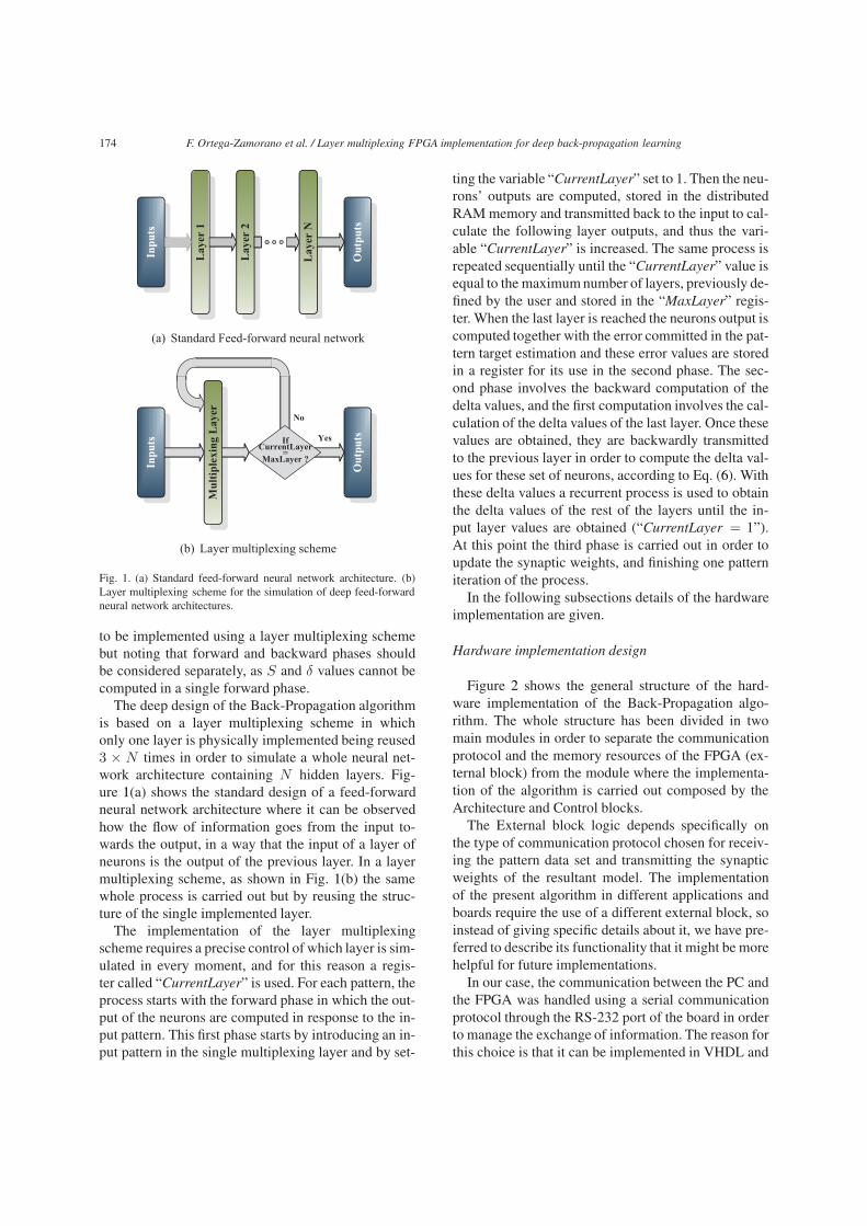
Fig. 4. Schematic representation of the layer multiplexing procedureused for the implementation of the BP algorithm.

network, sending back a signal (Ready_Train) to thecontrol block when the training of this pattern finishes,increasing the trained pattern counter Count1. Whenthe value of this counter gets equal to the total numberof training patterns, then the validation process start.The previous steps belong to a loop so they are re-peated until the maximum number of epochs (#Epoch)is reached.

3.2. Architecture block

The Fig. 4 shows a scheme of the architectureblock that performs the layer multiplexing procedureby physically implementing a single layer of neurons.This single layer is composed of A neurons blocks inparallel implemented in order to compute the neuron‘soutput (S) and the δ values, that will later be usedfor the update of the synaptic weights. The value ofA (limited by the board resources) will be the max-imum number of neurons for any hidden layer. Theneuron blocks manage their own synaptic weights in-dependently of the rest of the architecture, and thus

they require a RAM block attached to them. Details ofthe neuron blocks are described below in Section 3.2.The architecture block also includes memory blocks tostore the S and δ values computed for every layer andalso for the different input and output signals that aredescribed below.

The input signals are the pattern to be learned,the signal that indicates a new pattern is introduced(New_pattern), the configuration and control data sets,including also the S and δ values. The configurationdata set includes the parameters set by the user to spec-ify the neural network architecture, including the num-ber of hidden layers, the number of neurons in each ofthese layers, learning parameters, etc. The control dataset are signals that the control block needs for manag-ing the process of the algorithm to activate the rightprocedure in every moment. The output signals com-prise the output (S) and the δ values for every layer,the training error of the current pattern, and the readysignals for the validation and training processes whichare integrated in the control data set.

The maximum number of layers has been deter-mined by the size of the bus used to address the mul-tiplexing layer scheme. In order to have a compromisebetween the number of layers and used resources, wehave employed 7 bits in this bus, so the maximum num-ber of layers is 27−1 = 127. Also, the maximum num-ber of layers is delimited for the resources needed tostore the synaptic weights, according to the next equa-tion:

Ni ∗N1 +N1 ∗N2 + . . .+NL−1 ∗NL−2

< Available RAM (7)

where Ni is the number of inputs, N1 is the numberof neurons in the first layer, N2 those corresponding tothe second layer and so on.

Neuron block

Each of the A neuron blocks manages its own synap-tic weights, computing the S and δ values involved inthe Back-Propagation pattern updating procedure. Theword length to be chosen for representing the synap-tic weights would depend on the available resources,taking into account that obtaining a higher accuracyrequires a larger representation, which will imply anincrease in the number of LUTs per neuron (conse-quently a reduced number of available neurons) and adecrease in the maximum operation frequency of theboard. A synaptic weight is represented by a bit array


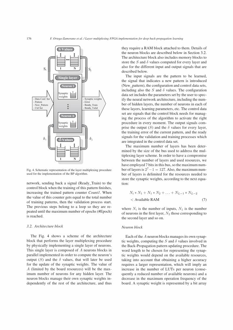
Table 1Board resources needed for the implementation of a neuron block

Registers LUTs DSPs RAM block

Neuron 428 1007 1 n =Avail.RAM#neurons

with integer and fractional parts of length N1 and N2.In our case the selected representation was N1 = 16and N2 = 16, a representation that permits a relativelyhigh accuracy as the errors generated in a layer arepropagated to further ones. Board resources needed forthe implementation of a neuron using the chosen rep-resentaion are shown in Table 1. The value for RAMblock shown in the last column of the table and indi-cated by n is equal to the available RAM (a value thatdepends on the FPGA board specifications) divided bythe maximum number of neurons allowed in the singleimplemented layer. For the implementation describedin this work n = 2 = int(14860 ) as the available RAM is148 blocks as indicated in Table 2, while the maximumnumber of neurons is 60 (see Section 5).

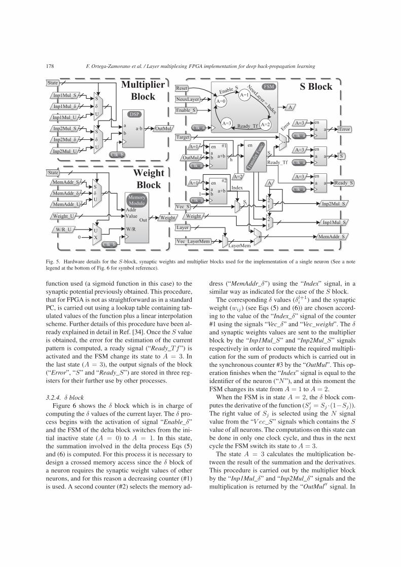
The implementation of the neuron blocks has beenperformed by dividing all the involved processes in fivemain sub-blocks (Multiplier, Weight S, δ and Updateblocks). We describe below the detailed implementa-tion of each one of these sub-blocks.

3.2.1. Multiplier blockThe multiplier block computes the multiplication

operations involved in the Back-Propagation algo-rithm, mainly between neuron activations and synapticweights values (see Eqs (1)–(6)). An efficient imple-mentation of this operation is crucial in order to opti-mize the board resources. A time-division multiplex-ing scheme has been developed for an efficient use ofthe resources, using only one multiplier per neuron andthus performing sequentially the computation of sev-eral products [34]. Multipliers can be implemented byshifters and adders, following the approach presentedin [4] or by available specific DSP cores in the FPGA.The DSP based strategy has been selected because thesystem frequency in the FPGA can be up to four timesfaster. The DSP uses a frequency two times larger thanthe used by the neuron block, so that a product opera-tion could be completed in one operation cycle of theFPGA.

Figure 5 shows the multiplier block. A “state” signalwill indicate which of the processes (S, δ or updating)is being executed at this moment, and two multiplex-ers will select the correct values to a DSP multiplier,which synchronized with a clock signal will send themultiplication result to the rest of the blocks.

3.2.2. Weight blockEach of the weight blocks attached to every neu-

ron is in charge of writing and reading the synapticweights using a single distributed RAM memory mod-ule. The memory module has three inputs (W/R, Addr,and Value) managed by two multiplexers controlled bythe signal “state”. The first input (W/R) decides whichaction to carry out (write or read), while the second in-put (Addr) specifies the memory address, and the thirdinputs is the value to store in case of a writing opera-tion. The first multiplexer (the bottom one in the fig-ure) allows writing (W/R = 1) only when the “state”signal is Update, otherwise only reading (W/R = 0) ispossible. The second multiplexer (the one on top) se-lects the address which will be used for the read/writeoperation according to the “state” signal (S, δ, U ). Thememory module also uses a frequency two times largerthan the used by the neuron block in order to completethe operation in one cycle of the FPGA.

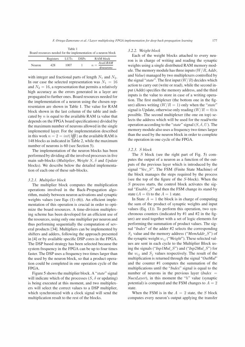
3.2.3. S blockThe S block (see the right part of Fig. 5) com-

putes the output of a neuron as a function of the out-puts of the previous layer which is introduced by thesignal “Vec_S”. The FSM (Finite State Machine) ofthe block manages the steps required by the process(see the top of the figure of the S-block). When theS process starts, the control block activates the sig-nal “Enable_S” and then the FSM change its stand-bystate (A = 0) to the A = 1 state.

In State A = 1 the block is in charge of computingthe sum of the product of synaptic weights and inputvalues (Eq. (1)). To perform this operation, two syn-chronous counters (indicated by #1 and #2 in the fig-ure) are used together with a set of logic elements forperforming the summation of product values. The sig-nal “Index” of the adder #2 selects the correspondingSj value and the memory address (“MemAddr_S”) ofthe synaptic weightwij (“Weight”). These selected val-ues are sent in each cycle to the Multiplier Block us-ing the signals (“Inp1Mul_S”) and (“Inp2Mul_S”) forthe wij and Sj values respectively. The result of themultiplication is returned through the signal “OutMul”and the counter #1 computes the summation of themultiplications until the “Index” signal is equal to thenumber of neurons in the previous layer (Index =NuexLayer), in this moment the “h” value (synapticpotential) is computed and the FSM changes to A = 2state.

When the FSM is in the A = 2 state, the S blockcomputes every neuron’s output applying the transfer


OutMul

NeuxLayer = Index

Vec_S

Layer

Vec_LayerMem

Index

LayerMem

Weight

A=1

A=2

A=0

enab a+b

h

1

S

A=1

enab a+b

A=1

Target

Ready_Tf

Inp1Mul_S

Inp2Mul_S

MemAddr_S

A

A=2

FSM

A=3Clk_a

Enable_SReset

NeuxLayer

-en

ena a Error

A=3

Clk_aError

ena a S

A=3

Clk_a

ena a Ready_S

A=3

Clk_a

+

21

21

Sj

A

ab

a·b

Sδ Inp1Mul_δ

Inp1Mul_S

Inp2Mul_S

Inp1Mul_U

Inp2Mul_U

Inp2Mul_δ

State

U

Sδ U

Clk_b

OutMul

DSP

Transfer Func.

Addr

W/R

Sδ MemAddr_δ

MemAddr_S

MemAddr_U

State

U

Clk_b

MemoryModule

UX

W/R_U0

WeightOut

S BlockMultiplierBlock

WeightBlock

Enable_S

#1

#2

Ready_Tf

Weight_U Value

Clk_a

Clk_a

Fig. 5. Hardware details for the S-block, synaptic weights and multiplier blocks used for the implementation of a single neuron (See a notelegend at the bottom of Fig. 6 for symbol reference).

function used (a sigmoid function in this case) to thesynaptic potential previously obtained. This procedure,that for FPGA is not as straightforward as in a standardPC, is carried out using a lookup table containing tab-ulated values of the function plus a linear interpolationscheme. Further details of this procedure have been al-ready explained in detail in Ref. [34]. Once the S valueis obtained, the error for the estimation of the currentpattern is computed, a ready signal (“Ready_Tf”) isactivated and the FSM change its state to A = 3. Inthe last state (A = 3), the output signals of the block(“Error”, “S” and “Ready_S”) are stored in three reg-isters for their further use by other processes.

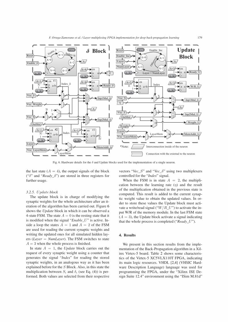
3.2.4. δ blockFigure 6 shows the δ block which is in charge of

computing the δ values of the current layer. The δ pro-cess begins with the activation of signal “Enable_δ”and the FSM of the delta block switches from the ini-tial inactive state (A = 0) to A = 1. In this state,the summation involved in the delta process Eqs (5)and (6) is computed. For this process it is necessary todesign a crossed memory access since the δ block ofa neuron requires the synaptic weight values of otherneurons, and for this reason a decreasing counter (#1)is used. A second counter (#2) selects the memory ad-

dress (“MemAddr_δ”) using the “Index” signal, in asimilar way as indicated for the case of the S block.

The corresponding δ values (δl+1i ) and the synaptic

weight (wij) (see Eqs (5) and (6)) are chosen accord-ing to the value of the “Index_δ” signal of the counter#1 using the signals “Vec_δ” and “Vec_weight”. The δand synaptic weights values are sent to the multiplierblock by the “Inp1Mul_S” and “Inp2Mul_S” signalsrespectively in order to compute the required multipli-cation for the sum of products which is carried out inthe synchronous counter #3 by the “OutMul”. This op-eration finishes when the “Index” signal is equal to theidentifier of the neuron (“N”), and at this moment theFSM changes its state from A = 1 to A = 2.

When the FSM is in state A = 2, the δ block com-putes the derivative of the function (S′

j = Sj ·(1−Sj)).The right value of Sj is selected using the N signalvalue from the “V ec_S” signals which contains the Svalue of all neurons. The computations on this state canbe done in only one clock cycle, and thus in the nextcycle the FSM switch its state to A = 3.

The state A = 3 calculates the multiplication be-tween the result of the summation and the derivatives.This procedure is carried out by the multiplier blockby the “Inp1Mul_δ” and “Inp2Mul_δ” signals and themultiplication is returned by the “OutMul′′ signal. In


A=4 A=3

Index=NA=1

A=0Enable_δ

∑

enab a+b

A=1Index

enaba+b

A=1

Index_δ

1N

enab a-b

A=1

1N

Vec_δ

Vec_Weight

Vec_S-

N

S

Layer

Vec_LayerMemLayerMem

+ MemAddr_δ

OutMul

1

Inp2Mul_δ

Inp1Mul_δ123

123

A

A=3 A=2

FSM

A=1A=0

Reset

A

Enable_Inc

Otherwise

Layer = NumLayer

Vec_S

Indexenab a+b

1

A=20

Vec_δ

η

OutMul

Weight+ Weight_U

Layer

Vec_LayerMemLayerMem + MemAddr_U

Inp1Mul_U

Inp2Mul_U

ena a Ready_U1

A=3

ena a1

A=3

12

12

Enable_Inc

Layer

NumLayer

Clk_a

Clk_aClk_a

Clk_a

S

δ

A=2

Enable_δ

ena a Ready_δ1

A=4

Clk_a

ena a δ

A=4

Clk_a

Clk_a

Clk_a

Clk_a

FSM

Resetδ Block Update

Block

A

0

*Note: Interconnection inside of the neuron

Connection with the external to the neuron

#1

W/R_U

#2#2 #3

A

Clk_a

Fig. 6. Hardware details for the δ and Update blocks used for the implementation of a single neuron.

the last state (A = 4), the output signals of the block(“δ” and “Ready_δ”) are stored in three registers forfurther usage.

3.2.5. Update blockThe update block is in charge of modifying the

synaptic weights for the whole architecture after an it-eration of the algorithm has been carried out. Figure 6shows the Update block in which it can be observed a4-state FSM. The state A = 0 is the resting state that itis modified when the signal “Enable_U” is active. In-side a loop the states A = 1 and A = 2 of the FSMare used for reading the current synaptic weights andwriting the updated ones for all simulated hidden lay-ers (Layer = NumLayer). The FSM switches to stateA = 3 when the whole process is finished.

In state A = 1, the Update block carries out therequest of every synaptic weight using a counter thatgenerates the signal “Index” for reading the storedsynaptic weights, in an analogous way as it has beenexplained before for the S Block. Also, in this state themultiplication between Si and δi (see Eq. (4)) is per-formed. Both values are selected from their respective

vectors “Vec_S” and “Vec_δ” using two multiplexerscontrolled for the “Index” signal.

When the FSM is in state A = 2, the multipli-cation between the learning rate (η) and the resultof the multiplication obtained in the previous state iscomputed. This result is added to the current synap-tic weight value to obtain the updated values. In or-der to store these values the Update block must acti-vate a write/read signal (“W/R_U”) to activate the in-put W/R of the memory module. In the last FSM state(A = 3), the Update block activate a signal indicatingthat the whole process is completed (“Ready_U”).

4. Results

We present in this section results from the imple-mentation of the Back-Propagation algorithm in a Xil-inx Virtex-5 board. Table 2 shows some characteris-tics of the Virtex-5 XC5VLX110T FPGA, indicatingits main logic resources. VHDL [2,4] (VHSIC Hard-ware Description Language) language was used forprogramming the FPGA, under the “Xilinx ISE De-sign Suite 12.4” environment using the “ISim M.81d”


Table 2Main specifications of the Xilinx Virtex-5 XC5VLX110T FPGAboard

Device Slice Slice Bonded BlockRegisters LUTs IOBs RAM

Virtex-5 69, 120 69, 120 34 148XC5VLX110T

simulator. The operation system frequency was in-creased from the 100 MHZ board oscillator frequencyto 200 MHZ through the use of a PLL, as the efficiencyof the code allowed this configuration.

To verify the correct FPGA implementation of themodel, several test cases were analyzed comparing theresults with those obtained from C and Matlab imple-mentations and with previously published results. Inparticular, to assess the advantages of using an FPGAboard, we compare the results testing several networkarchitectures under C and Matlab programming lan-guages executed in the Picasso cluster that belongs tothe Spanish Supercomputing Network.1 The cluster isformed by a set of computation nodes unified behind asingle Slurm queue system, consisting mainly of 7 HPDL980 nodes of 80 cores and 2 TB RAM computers,32 HP SL230 nodes with 16 cores and 64 GB of RAM,42 HP DL165 nodes with 24 cores and 96 GB of RAM,and 16 HP SL250 nodes with 2 GPUs each, totalling63 TFLOP/s. Own generated code in C and Matlablanguages were used for the comparison, noting thatthe C programming language is considered among thefastest that can be used in a PC [7,16] while Matlab isa language optimized for operations involving matri-ces and vectors useful for neural network implementa-tions [27,42]. All the tests were carried out using a 50-20-30 splitting for the training, validation and general-ization sets respectively, with a learning rate (η) valuefixed to 0.2, and using data from the well-known Irisset [28]. The generalization set contains only patternsnot used during the learning process, and it is used totest the prediction capacity of the algorithm, known asGeneralization ability (Gen).

Figure 7 shows the evolution for the training (Etr)and validation (Eval) errors for the FPGA and the mul-ticore (MC) cluster based implementation. The archi-tectures used contained one hidden layer (a), two (b),and three (c), including five neurons in all hidden lay-ers, and three neurons in the output that corresponds tothe three classes of the Iris problem. In all three graphs,two vertical lines indicate the time at which the mini-

1http://www.scbi.uma.es/.

0 100 200 300 400 500 600 700 800 900 1000Number of epochs

0

0.1

0.2

0.3

0.4

Mea

n sq

uare

err

or

A Gen FPGA = 0.87A Gen MC= 0.9

FPGA EtrFPGA EvalMC EtrMC Evalmin(FPGA Eval)min(MC Eval)

(a) One hidden layer

0 100 200 300 400 500 600 700 800 900 1000Number of epochs

0

0.1

0.2

0.3

0.4

Mea

n sq

uare

err

or

A Gen FPGA = 0.97A Gen MC= 0.933


(b) Two hidden layers

0 100 200 300 400 500 600 700 800 900 1000Number of epochs

0

0.1

0.2

0.3

0.4

Mea

n sq

uare

err

or

Gen FPGA = 0.97!Gen MC= 0.967!


(c) Three hidden layers

Fig. 7. Training (Etr) and validation (Eval) errors evolution for thetwo implementations (FPGA, MC) when the Iris data set is learneddepending on the number of layer of the neural architecture with fiveneurons in each hidden layer.

mum of the validation error is obtained, point when theGeneralization ability (Gen) is measured for both im-plementations (the obtained values are also indicated inthe graph). It can be appreciated from the error curvesthat for the FPGA implementation case some larger os-cillations appear, and this is due to rounding effectsbecause of the size of the fixed point representationused. In terms of the level of prediction accuracy ob-tained these oscillations do not degrade it, and on thecontrary in some cases even leads to larger values, asit has been observed previously in FPGA implementa-tions [31,33], and in several works where it was con-cluded that certain level of noise might be beneficialfor improving learning times, fault tolerance and pre-diction accuracy [1,15,26].


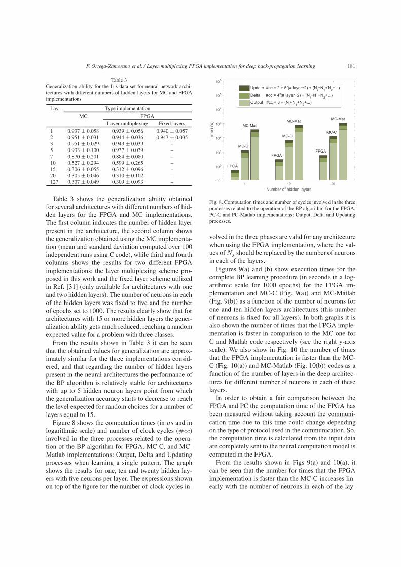
Table 3Generalization ability for the Iris data set for neural network archi-tectures with different numbers of hidden layers for MC and FPGAimplementations

Lay. Type implementationMC FPGA

Layer multiplexing Fixed layers1 0.937 ± 0.058 0.939 ± 0.056 0.940 ± 0.0572 0.951 ± 0.031 0.944 ± 0.036 0.947 ± 0.0353 0.951 ± 0.029 0.949 ± 0.039 –5 0.933 ± 0.100 0.937 ± 0.039 –7 0.870 ± 0.201 0.884 ± 0.080 –10 0.527 ± 0.294 0.599 ± 0.265 –15 0.306 ± 0.055 0.312 ± 0.096 –20 0.305 ± 0.046 0.310 ± 0.102 –127 0.307 ± 0.049 0.309 ± 0.093 –

Table 3 shows the generalization ability obtainedfor several architectures with different numbers of hid-den layers for the FPGA and MC implementations.The first column indicates the number of hidden layerpresent in the architecture, the second column showsthe generalization obtained using the MC implementa-tion (mean and standard deviation computed over 100independent runs using C code), while third and fourthcolumns shows the results for two different FPGAimplementations: the layer multiplexing scheme pro-posed in this work and the fixed layer scheme utilizedin Ref. [31] (only available for architectures with oneand two hidden layers). The number of neurons in eachof the hidden layers was fixed to five and the numberof epochs set to 1000. The results clearly show that forarchitectures with 15 or more hidden layers the gener-alization ability gets much reduced, reaching a randomexpected value for a problem with three classes.

From the results shown in Table 3 it can be seenthat the obtained values for generalization are approx-imately similar for the three implementations consid-ered, and that regarding the number of hidden layerspresent in the neural architectures the performance ofthe BP algorithm is relatively stable for architectureswith up to 5 hidden neuron layers point from whichthe generalization accuracy starts to decrease to reachthe level expected for random choices for a number oflayers equal to 15.

Figure 8 shows the computation times (in μs and inlogarithmic scale) and number of clock cycles (#cc)involved in the three processes related to the opera-tion of the BP algorithm for FPGA, MC-C, and MC-Matlab implementations: Output, Delta and Updatingprocesses when learning a single pattern. The graphshows the results for one, ten and twenty hidden lay-ers with five neurons per layer. The expressions shownon top of the figure for the number of clock cycles in-

1 10 20Number of hidden layers

10-1

100

101

102

103

104

105

106

Tim

e (7

s)

FPGA

MC-C

MC-Mat

FPGA

MC-C

MC-Mat

FPGA

MC-C

MC-Mat

Update #cc = 2 + 5"(# layer+2) + (Ni+N

1+N

2+...)

Delta #cc = 4"(# layer+2) + (Ni+N

1+N

2+...)

Output #cc = 3 + (Ni+N

1+N

2+...)

Fig. 8. Computation times and number of cycles involved in the threeprocesses related to the operation of the BP algorithm for the FPGA,PC-C and PC-Matlab implementations: Output, Delta and Updatingprocesses.

volved in the three phases are valid for any architecturewhen using the FPGA implementation, where the val-ues of Nj should be replaced by the number of neuronsin each of the layers.

Figures 9(a) and (b) show execution times for thecomplete BP learning procedure (in seconds in a log-arithmic scale for 1000 epochs) for the FPGA im-plementation and MC-C (Fig. 9(a)) and MC-Matlab(Fig. 9(b)) as a function of the number of neurons forone and ten hidden layers architectures (this numberof neurons is fixed for all layers). In both graphs it isalso shown the number of times that the FPGA imple-mentation is faster in comparison to the MC one forC and Matlab code respectively (see the right y-axisscale). We also show in Fig. 10 the number of timesthat the FPGA implementation is faster than the MC-C (Fig. 10(a)) and MC-Matlab (Fig. 10(b)) codes as afunction of the number of layers in the deep architec-tures for different number of neurons in each of theselayers.

In order to obtain a fair comparison between theFPGA and PC the computation time of the FPGA hasbeen measured without taking account the communi-cation time due to this time could change dependingon the type of protocol used in the communication. So,the computation time is calculated from the input dataare completely sent to the neural computation model iscomputed in the FPGA.

From the results shown in Figs 9(a) and 10(a), itcan be seen that the number for times that the FPGAimplementation is faster than the MC-C increases lin-early with the number of neurons in each of the lay-


1 2 3 4 5 6 7 8 9 10 11 12# Neurons

10-3

10-2

10-1

100

101

102

103

Tim

e(s)

051015202530

50

100

# Ti

mes

#times 1 layer#times 10 layer

Time FPGA 1 LayerTime FPGA 10 LayerTime MC-C 1 LayerTime MC-C 10 Layer

(a)

1 2 3 4 5 6 7 8 9 10 11 12# Neurons

10-3

10-2

10-1

100

101

102

103

Tim

e(s)

0

250

500

750

1000

1250

1500

1750

2000#

Tim

es

#times 1 layer#times 10 layer

Time FPGA 1 LayerTime FPGA 10 LayerTime MC-Mat 1 LayerTime MC-Mat 10 Layer

(b)

Fig. 9. Computational time and number of times that the FPGA im-plementation is faster than the MC-C (a) and MC-Matlab (b) as afunction of the number of neurons in each layer for the case of oneand ten hidden layers architectures (see text for details).

ers, reaching 27 times for the case of using 60 neuronsin each layer, noting that these values are kept con-stant for different number of hidden layers. In relation-ship to the computational times between the FPGA andthe MC-Matlab implementation the advantage of us-ing the FPGA decreases as the number of neurons ineach layer increases, and this effect can be explainedbecause Matlab uses matrix-based computations thatare more efficient for heavier computations, but notingthat the number of times that the FPGA is faster thanMC-Matlab converges asymptotically to 60 times ap-proximately.

To test the correct implementation of the deep learn-ing scheme of the BP algorithm in the FPGA board,we measured training, validation and test errors on aset of benchmark problems from the UCI database [28]frequently used in the literature. Table 4 shows the ac-curacy (generalization ability) values obtained for bothimplementations of the algorithm for eleven bench-

Table 4Generalization ability for PC and FPGA implementations obtainedfor eleven benchmark data sets

Function I O PC FPGADiabetes 8 2 0.784 ± 0.028 0.793 ± 0.023Cancer 9 2 0.958 ± 0.013 0.954 ± 0.011Statlog 13 2 0.784 ± 0.023 0.776 ± 0.022Climate 18 2 0.933 ± 0.012 0.944 ± 0.015Ionosphere 34 2 0.874 ± 0.001 0.864 ± 0.001HeartC 35 2 0.789 ± 0.035 0.801 ± 0.028Iris 4 3 0.923 ± 0.019 0.926 ± 0.020Bal.Sca. 4 3 0.869 ± 0.011 0.873 ± 0.012Seeds 7 3 0.976 ± 0.017 0.965 ± 0.016Wine 13 3 0.886 ± 0.022 0.880 ± 0.024Glass 10 6 0.938 ± 0.025 0.914 ± 0.022

Average 0.8830 ± 0.0187 0.8808 ± 0.0176

1 2 3 4 5 6 7 8 9 10 11 12 13 14 15 16 17 18 19 20# Layers

10

15

20

25

30

# Ti

mes

# Neurons:51015202530354045505560

(a)

1 2 3 4 5 6 7 8 9 10 11 12 13 14 15 16 17 18 19 20# Layers

0

250

500

750

1000

1250

1500

# Ti

mes

# Neurons:

58.8

51015202530354045505560

(b)

Fig. 10. Number of times that the FPGA implementation is fasterthan the MC-C (graph a) and MC-Matlab (graph b) as a function ofthe number of layers in the deep architectures for different values forthe number of neurons in each of these layers.

mark problems. The first three columns indicate thedata set name, number of inputs and outputs respec-tively, while the last two columns shows the general-ization ability obtained using neural network architec-tures with 5 neurons in the single hidden layer. Thischoice of number of neurons permits the comparisonwith published results [31]. For carrying out the simu-lations a training, validation and test sets splitting was


used in a 50-20-30% scheme; in which the validationset was used to find the number of epochs for evaluat-ing the test error, the maximum number of epochs wasset to 1000, and the learning rate was equal to 0.2. 100independent runs were computed for each benchmarkdata set and the average and standard deviation of theobtained results are reported in the table. The resultsindicate a correct functioning of the algorithm, notingthat the small observed differences can be related tothe methodology of computation and to the differentnumber representation used in the two analyzed cases.

5. Discussion and conclusions

We have successfully implemented the Back Propa-gation algorithm in an FPGA board using a novel layermultiplexing on-chip learning scheme that includes avalidation procedure in order to prevent overfitting ef-fects. The layer multiplexing scheme utilized permitsto simulate a several hidden layer neural network withonly implementing physically a single hidden layer ofneurons. The main advantage of this approach is thatvery deep neural network architectures can be analyzedthrough a simple and flexible framework with very ef-ficient resource utilization. A modular design has beenutilized in a hardware implementation that incorpo-rates strategies like multiplexing of the multipliers, op-timized memory access and efficient data type repre-sentation, with the aim of producing a flexible and re-source efficient tool for the study of multi-layer neuralarchitectures.

In terms of computational times, the implementa-tion has been tested and compared to multicore (MC)C and Matlab codes executed in a 97 nodes supercom-puter. In comparison to the MC-C code, the number oftimes that the FPGA implementation is faster increaseslinearly as the number of neurons in each of the lay-ers increases, while being almost constant for differentnumber of hidden layers, reaching a value of 27 when60 neurons are included in each of these hidden lay-ers. The same comparison but for the case of FPGAand MC-Matlab implementations shows a different be-haviour as the advantage of the FPGA decreases as thenumber of neurons in each layer increases. This advan-tage also has a slight decrease as the number of layersis increased, but in all analyzed cases being larger than58.8 times.

The layer multiplexing scheme used permits inprinciple the simulation of networks with any num-ber of hidden layers, but due to memory resource

design the maximum number of layers in the cur-rent implementation is 127. Regarding the maximumnumber of neurons allowed in each of the hiddenlayer, hardware resources of the FPGA board used(VIRTEX-5 XC5VLX110T) pose a limit of 60 neu-rons. The results obtained confirm the degradation ofthe Back-Propagation algorithm for very deep archi-tectures comprising 15 or more hidden layers, as al-most a random behavior is obtained for deeper net-works (see Table 3). Understanding and improving thetraining of deep architectures is a big present chal-lenge, and we believe that the present work may con-tribute to their understanding as we have introduceda flexible tool for carrying this analysis that we planto tackle in the near future. Further, it is worth notingthat so far FPGAs have not been much applied to DeepLearning approaches, and we believe that high devel-oping times are to blame. In this sense, we hope thatthis work can help other researchers on the applicac-tion of FPGA based approaches, as the intrinsic paral-lelism of these devices makes them a suitable technol-ogy for implementing neuroinspired models.

Acknowledgments

The authors acknowledge support from Junta de An-dalucia through grant P10-TIC-5770, and from CICYT(Spain) through grants TIN2010-16556 and TIN2014-58516-C2-1-R (all including FEDER funds). The au-thors thankfully acknowledge the computer resources,technical expertise and assistance provided by theSCBI (Supercomputing and Bioinformatics) center ofthe University of Málaga, Spain.

Appendix

Detail of signals used between blocks (see Fig. 2 andrelated text)

– Ready_Patterns: Active (‘1’) when the patterndata set is ready to be learned.

– New_Valid: A pulse (one clock cycle active)when a validation pattern is required for the archi-tecture.

– New_Train: A pulse when a training pattern is re-quired for the architecture.

– V_T: A signal which defines the process (valida-tion or training) that is being executed.

– Enable_Sent: A pulse when the stored synapticweights in the external block must be send fromthe external block to the user.


– Enable_Store: A pulse when the synaptic weightsof the neurons must be stored in the externalblock.

– End: Active when the process is finished.– Ready_Sent: A pulse that is sent when the ex-

ternal block has finished sending the synapticweights to the external device.

– Ready_Store: A pulse that is sent when the exter-nal block has finished storing the synaptic weightsof every neuron.

– Data_Conf_Set: Variables of configuration of themodel (number of layers, number of neuron forlayer, number of patterns, etc).

– Pattern: Variable that introduces a new training orvalidation pattern when New_Train or New_Validis active. respectively.

– New_Pattern: Pulse when a pattern is introduced.– Weights: Synaptic weights of every neuron to be

stored.

References

[1] G. An, The effects of adding noise during backpropagationtraining on a generalization performance, Neural Computa-tion 8(3) (Apr 1996), 643–674.

[2] P. Ashenden, The Designer’s Guide to VHDL, Volume 3, ThirdEdition (Systems on Silicon) (Systems on Silicon), 3 edition,Morgan Kaufmann Publishers Inc., San Francisco, CA, USA,2008.

[3] Y. Bengio, P. Simard and P. Frasconi, Learning long-term de-pendencies with gradient descent is difficult, IEEE Transac-tions on Neural Networks 5(2) (Mar 1994), 157–166.

[4] P.P. Chu, RTL Hardware Design Using VHDL: Coding forEfficiency, Portability, and Scalability, John Wiley & Sons,2006.

[5] C. Clark and A.J. Storkey, Training deep convolutional neu-ral networks to play go, in: Proceedings of the 32nd Interna-tional Conference on Machine Learning, volume 37 of JMLRProceedings, JMLR.org (2015), 1766–1774.

[6] A. Dinu, M. Cirstea and S. Cirstea, Direct neural-networkhardware-implementation algorithm, IEEE Transactions onIndustrial Electronics 57(5) (May 2010), 1845–1848.

[7] B. Fulgham, The computer language benchmarks game, http://benchmarksgame.alioth.debian.org/.

[8] X. Glorot and Y. Bengio, Understanding the difficulty of train-ing deep feedforward neural networks, in: Proceedings ofthe International Conference on Artificial Intelligence andStatistics (AISTATS’10), Society for Artificial Intelligence andStatistics, (2010), 249–256.

[9] A. Gomperts, A. Ukil and F. Zurfluh, Development and imple-mentation of parameterized fpga-based general purpose neu-ral networks for online applications, IEEE Transactions onIndustrial Informatics 7(1) (Feb 2011), 78–89.

[10] B. Guthier, S. Kopf, M. Wichtlhuber and W. Effelsberg,Parallel implementation of a real-time high dynamic rangevideo system, Integrated Computer-Aided Engineering 21(2)(2014), 189–202.

[11] D.M. Hawkins, The problem of overfitting, Journal of Chem-ical Information and Computer Sciences 44(1) (2004), 1–12.

[12] S. Haykin, Neural Networks: A Comprehensive Foundation,2nd edition, Prentice Hall PTR, Upper Saddle River, NJ,USA, 1998.

[13] S. Himavathi, D. Anitha and A. Muthuramalingam, Feedfor-ward neural network implementation in fpga using layer mul-tiplexing for effective resource utilization, IEEE Transactionson Neural Networks 18(3) (May 2007), 880–888.

[14] G.E. Hinton, S. Osindero and Y.-W. Teh, A fast learning algo-rithm for deep belief nets, Neural Comput 18(7) (July 2006),1527–1554.

[15] L. Holmstrom and P. Koistinen, Using additive noise in back-propagation training, Neural Networks, IEEE Transactions on3(1) (Jan 1992), 24–38.

[16] R. Hundt, Loop recognition in c++/java/go/scala, in: Proceed-ings of Scala Days 2011, (2011).

[17] F. Iandola, K. Ashraf, M. Moskewicz and K. Keutzer, Fire-caffe: Near-linear acceleration of deep neural network train-ing on compute clusters, in: Proceeedings of the 2016 IEEEConference on Computer Vision and Pattern Recognition(CVPR).

[18] S. Kilts, Advanced FPGA Design: Architecture, Implementa-tion, and Optimization, Wiley-IEEE Press, 2007.

[19] L.-W. Kim, S. Asaad and R. Linsker, A fully pipelined fpgaarchitecture of a factored restricted boltzmann machine artifi-cial neural network, ACM Trans Reconfigurable Technol Syst7(1) (Feb 2014), 5–23.

[20] Q.N. Le and J.-W. Jeon, Neural-network-based low-speed-damping controller for stepper motor with an fpga, IEEETransactions on Industrial Electronics 57(9) (Sept 2010),3167–3180.

[21] D. LeLy and P. Chow, High-performance reconfigurable hard-ware architecture for restricted boltzmann machines, IEEETransactions on Neural Networks 21(11) (Nov 2010), 1780–1792.

[22] Y. LeCun, Y. Bengio and G. Hinton, Deep learning, Nature521(7553) (May 2015), 436–444.

[23] J. Li, K. Ouazzane, H. Kazemian and M. Afzal, Neural net-work approaches for noisy language modeling, Neural Net-works and Learning Systems, IEEE Transactions on 24(11)(Nov 2013), 1773–1784.

[24] W. Mansour, R. Ayoubi, H. Ziade, R. Velazco and W.E.Falouh, An optimal implementation on fpga of a hopfieldneural network, Advances in Artificial Neural Systems 2011(2011), 1–9.

[25] K. Mehrotra, C.K. Mohan and S. Ranka, Elements of ArtificialNeural Networks, MIT Press, Cambridge, MA, USA, 1997.

[26] A. Murray and P. Edwards, Synaptic weight noise during mul-tilayer perceptron training: Fault tolerance and training im-provements, Neural Networks, IEEE Transactions on 4(4) (Jul1993), 722–725.

[27] J. Nazari and O.K. Ersoy, Implementation of back-propagation neural networks with matlab, Technical report,Purdue University School of Electrical Engineering (011992).

[28] U. of California Irvine, Machine learning repository, http://archive.ics.uci.edu/ml/.

[29] A. Omondi and J. Rajapakse, FPGA Implementations of Neu-ral Networks, Springer-Verlag New York, Inc., Secaucus, NJ,USA, 2006.

[30] T. Orlowska-Kowalska and M. Kaminski, Fpga implementa-tion of the multilayer neural network for the speed estimationof the two-mass drive system, IEEE Transactions on Indus-


trial Informatics 7(3) (Aug 2011), 436–445.[31] F. Ortega-Zamorano, J.M. Jerez, D. Urda Muñoz, R.M.

Luque-Baena and L. Franco, Efficient implementation ofthe backpropagation algorithm in fpgas and microcontrollers,IEEE Transactions on Neural Networks and Learning Systems27(9) (2016), 1840–1850.

[32] F. Ortega-Zamorano, J.M Jerez and L. Franco, Fpga imple-mentation of the c-mantec neural network constructive al-gorithm, IEEE Transactions on Industrial Informatics 10(2)(May 2014), 1154–1161.

[33] F. Ortega-Zamorano, J.M Jerez, G. Juarez and L. Franco, Fpgaimplementation comparison between c-mantec and back-propagation neural network algorithms, in: Advances in Com-putational Intelligence, volume 9095, Springer InternationalPublishing, (2015), 197–208.

[34] F. Ortega-Zamorano, J.M Jerez, G. Juarez, J.O Pérez and L.Franco, High precision fpga implementation of neural net-work activation functions, in: Intelligent Embedded Systems(IES), 2014 IEEE Symposium on, (Dec 2014), 55–60.

[35] T. Pinto, Z. Vale, T.M. Sousa, I. Praça, G. Santos and H.Morais, Adaptive learning in agents behaviour: A frameworkfor electricity markets simulation, Integr Comput-Aided Eng21(4) (Oct 2014), 399–415.

[36] R.D. Reed and R.J. Marks, Neural Smithing: SupervisedLearning in Feedforward Artificial Neural Networks, MITPress, Cambridge, MA, USA, 1998.

[37] M. Rizzi, M. D’Aloia and B. Castagnolo, A super-vised method for microcalcification cluster diagnosis, IntegrComput-Aided Eng 20(2) (Apr 2013), 157–167.

[38] D. Rumelhart, G. Hinton and R. Williams, Learning represen-tations by back-propagating errors, Nature 323(6088) (1986),533–536.

[39] A. Savich, M. Moussa and S. Areibi, The impact of arithmeticrepresentation on implementing mlp-bp on fpgas: A study,IEEE Transactions on Neural Networks 18(1) (Jan 2007),240–252.

[40] J. Schmidhuber, Deep learning in neural networks: Anoverview, Neural Networks 61 (2015), 85–117.

[41] J. Shawash and D. Selviah, Real-time nonlinear parameterestimation using the levenberg-marquardt algorithm on fieldprogrammable gate arrays, IEEE Transactions on IndustrialElectronics 60(1) (Jan 2013), 170–176.

[42] S. Shrestha, Z. Bochenek and C. Smith, Artificial neural net-work (ann) beyond cots remote sensing packages: Imple-mentation of extreme learning machine (elm) in matlab, in:Geoscience and Remote Sensing Symposium (IGARSS), 2012IEEE International, (July 2012), 6301–6304.

[43] S. Sun, Z. Yan and J. Zambreno, Demonstrable differentialpower analysis attacks on real-world fpga-based embeddedsystems, Integr Comput-Aided Eng 16(2) (Apr 2009), 119–130.

[44] N. Sundararajan and P. Saratchandran, Parallel Architecturesfor Artificial Neural Networks: Paradigms and Implementa-tions, 1st edition, IEEE Computer Society Press, Los Alami-tos, CA, USA, 1998.

[45] H. Wen, W. Xie and J. Pei, A pre-radical basis function withdeep back propagation neural network research, in: SignalProcessing (ICSP), 2014 12th International Conference on,(Oct 2014), 1489–1494.

[46] P.J. Werbos, Beyond regression: New tools for prediction andanalysis in the behavioral sciences, Ph.D. thesis, Harvard Uni-versity, 1974.

Integrated Computer-Aided Engineering 24 (2017) 171–185 ...

Documents