Instance Segmentation of Fibers from Low Resolution CT ...

KONOPCZYNSKI et al.: FIBER INSTANCE SEGMENTATION FROM CT VIA DL 1

Instance Segmentation of Fibersfrom Low Resolution CT Scansvia 3D Deep Embedding Learning

Tomasz Konopczynski∗13

[email protected]

Thorben Kröger2

[email protected]

Lei Zheng1

[email protected]

Jürgen Hesser1

[email protected]

1 Department of Radiation OncologyUniversity Medical Center MannheimHeidelberg University, Germany

2 Volume GraphicsHeidelberg, Germany

3 TooplooxWrocław, Poland

Abstract

We propose a novel approach for automatic extraction (instance segmentation) offibers from low resolution 3D X-ray computed tomography scans of short glass fiberreinforced polymers. We have designed a 3D instance segmentation architecture builtupon a deep fully convolutional network for semantic segmentation with an extra outputfor embedding learning. We show that the embedding learning is capable of learning amapping of voxels to an embedded space in which a standard clustering algorithm can beused to distinguish between different instances of an object in a volume. In addition, wediscuss a merging post-processing method which makes it possible to process volumesof any size. The proposed 3D instance segmentation network together with our mergingalgorithm is the first known to authors knowledge procedure that produces results goodenough, that they can be used for further analysis of low resolution fiber composites CTscans.

1 IntroductionReliable information about fiber characteristics in short-fiber reinforced polymers (SFRP) ismuch needed for process optimization during the product development phase. The influenceof fiber characteristics on the mechanical properties of SFRP composites is of particular in-terest and significance for manufacturers [9]. The recent development of X-ray computedtomography (CT) for nondestructive quality control enabled the possibility to scan the ma-terials and retrieve the 3D spatial information of SFRPs. Fiber extraction is the first steptowards any further analysis of a SFRP material. However, the spatial resolution of a scan isa limiting factor which makes fiber extraction a difficult problem.

Acquiring scans in high resolution is time consuming and costly. Therefore, in this workwe consider only scans acquired by a CT system with low (3.9 µm) resolution. The methods

c© 2018. The copyright of this document resides with its authors.It may be distributed unchanged freely in print or electronic forms.

∗ work done while at Volume Graphics.

arX

iv:1

901.

0103

4v1

[cs

.CV

] 4

Jan

201

9

2 KONOPCZYNSKI et al.: FIBER INSTANCE SEGMENTATION FROM CT VIA DL

Figure 1: Sketch of the proposed method. The network is processing overlapping sub-volumes of the input volume. For each sub-volume a semantic segmentation mask and anembedding is produced by a deep network. A clustering method is then applied on thesegmented regions of the embedding representation producing clusters corresponding to in-dividual fibers. Fibers are then mapped back to the spatial domain. The overlapping instancesub-volumes are then merged into an output volume.

currently in use are usually based on hand designed features. Since fibers can be described aslong cylindrically shaped objects, the most widely used family of fully-automatic methodsis based on Hessian eigenvalues. Using a set of Hessian based filters at a number of scales,a confidence map of fiber occurrence can be produced [8]. To extract individual fibers, atemplate matching [21] [6] or a watershed splitting and skeletonisation technique [24] [26] isthen applied. However, the performance of these methods degrades severely if the resolutionis too low and fails to produce meaningful results [15]. A deep learning method has alreadyshown its superiority over Hessian based techniques to produce more accurate results forsemantic segmentation of fibers at low CT resolution [16].

Deep learning architectures have been successfully applied to semantic segmentationproblems for both natural 2D images and 3D CT volumes [18] [3]. Similar solutions havebeen found for the problem of 2D instance segmentation. Faster R-CNN [22] and the MaskR-CNN [11] architectures are examples of region-proposal-based techniques which are thestate-of-the-art for common scene-understanding datasets like COCO [17] or ImageNet [4].However, it is not clear how this approach can be extended to 3D volumetric data withdensely packed objects like fibers in SFRP. This is why for our 3D problem, we have optedfor alternative deep learning methods for instance segmentation. There are numerous worksin which authors try to come up with different ideas for 2D datasets. An interesting ideathat could be extended to 3D volumes has been proposed by [1] to reformulate the problemof instance segmentation into learning a mapping to watershed energy. Then, for the finaloutput, a Watershed transform is applied to get the instances. Unfortunately, this methodis not applicable to our problem, because fibers are usually too thin to find a border. An-other promising idea proposed by [23] is to combine convolutional neural networks (CNN)with recurrent neural networks (RNN). The recurrent structures are used to keep track ofobjects that have already been found, and excludes these regions from further analysis by thealgorithm.

In this work we propose a novel deep learning architecture for automatic extraction (in-stance segmentation) of fibers from low resolution 3D X-ray computed tomography scans ofshort glass fiber reinforced polymers. The sketch of the method is presented in Fig. 1.

KONOPCZYNSKI et al.: FIBER INSTANCE SEGMENTATION FROM CT VIA DL 3

(a) (b) (c) (d)Figure 2: Visualization of the network outputs. (a) Slice of an input volume patch. (b) Corre-sponding slice from the semantic segmentation output. (c) Corresponding slice of one (out ofmany) feature map of the embedding output. The network learns to assign different, uniquevalues (colors) to individual fibers. In this particular feature map all fibers are well separated.(d) The masked embedding by a semantic prediction for which a loss for embedding learningis computed. In the prediction phase it is also the input for the clustering step.

We explore and discuss the performance of the presented method achieved by trainingon a low resolution SFRP CT scan and compare it to a standard watershed splitting andskeletonisation technique. We test the importance of the semantic segmentation branch byreplacing it with a ground truth semantic segmentation. To the best of our knowledge, this isthe first attempt of using deep embedding learning for the task of instance segmentation ona 3D volumetric data. The proposed method is also the first to successfully retrieve single-fiber segmentation from a low resolution SFRP CT scan, while the outcome of the standardmethods is producing unacceptable results. We base our method on an embedding learningapproach [25] [2]. The idea is to use a special embedding layer which is placed at theend of a given deep network. The network is then trained by using a special loss functionon the final embedding layer which encourages special structure in the embedding space:pixels belonging to the same class should be close, whereas pixels belonging to differentclasses should be far apart (in the Euclidean metric of the embedding space). The methodas a learnable loss function has been first mentioned by [25], and was then used with somemodifications in the deep learning architecture of [2] and [7]. These methods achievedcompetitive performance on 2D datasets compared with the R-CNN based state-of-the-art.

In the problem of fiber segmentation, the network will learn a mapping of each voxel andits surrounding from the input to an embedding space in which voxels belonging to one fiberare separated from voxels belonging to another. Unfortunately, there is one drawback to thismethod. Such a network is capable of processing only one small sub-volume of a volumeat a time because of memory limitation. Each time the network processes a sub-volume itassigns an arbitrary index to a fiber region. Because of that, we can not do a simple mergeas it is usually done for a semantic segmentation problem, where the output is a probabilityof being an object of a certain class. For a semantic segmentation mask one can take asimple average over overlapping regions in order to merge sub-volumes into a full volume.Therefore, in order to produce an instance segmentation for a full CT scan, we propose apost-processing algorithm, which merges the overlapping predictions of small blocks into aconsistent prediction for the entire CT scan during the prediction phase.

2 MethodSimilar to the work of [2], we have extended the Fully Convolutional Network (FCN) archi-tecture [18] designed for semantic segmentation tasks to produce embeddings by using an

4 KONOPCZYNSKI et al.: FIBER INSTANCE SEGMENTATION FROM CT VIA DL

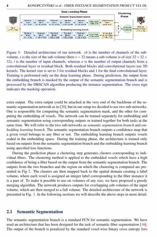
Figure 3: Detailed architecture of our network. ch is the number of channels of the sub-volume, s is the size of the sub-volume (here s = 32 means a sub-volume is of size 32×32×32), i is the number of input channels, whereas o is the number of output channels from aconvolutional layer or residual block. Both residual blocks and convolutional layers use 3Dkernels. The kernel size is set to 3 for residual blocks and 1 for the final convolutional layer.Training is performed only on the deep learning phase. During prediction, the output fromthe embedding branch is masked by the output of the semantic segmentation branch and isprocessed by the DBSCAN algorithm producing the instance segmentation. The cross signindicates the masking operation.

extra output. The extra output could be attached at the very end of the backbone of the se-mantic segmentation network as in [20], but in our setup we decided to use two sub-networks.One is responsible for computing the semantic segmentation mask, and the other for com-puting the embedding of voxels. The network can be trained separately for embedding andsemantic segmentation using corresponding outputs or trained together for both tasks at thesame time. We will refer to the two sub-networks as semantic segmentation branch and em-bedding learning branch. The semantic segmentation branch outputs a confidence map thata given voxel belongs to any fiber or not. The embedding learning branch outputs voxelscoded in the embedding space. During the training phase, the architecture is trained onlybased on outputs from the semantic segmentation branch and the embedding learning branchusing specified loss functions.

During the prediction phase a clustering step generates clusters corresponding to indi-vidual fibers. The clustering method is applied to the embedded voxels which have a highconfidence of being a fiber based on the output from the semantic segmentation branch. Theoutputs from the two branches and the region on which the clustering is computed are pre-sented in Fig 2. The clusters are then mapped back to the spatial domain creating a labelvolume, where each voxel is assigned an integer label corresponding to the fiber instance itis a part of. To make it possible to use on volumes of any size, we have proposed a greedymerging algorithm. The network produces outputs for overlapping sub-volumes of the inputvolume, which are then merged to a full volume. The detailed architecture of the network ispresented in Fig. 3. In the following sections we will describe the above steps in more detail.

2.1 Semantic Segmentation

The semantic segmentation branch is a standard FCN for semantic segmentation. We haveused an architecture that has been designed for the task of semantic fiber segmentation [16].The output of the branch is penalized by the standard voxel-wise binary cross entropy loss

KONOPCZYNSKI et al.: FIBER INSTANCE SEGMENTATION FROM CT VIA DL 5

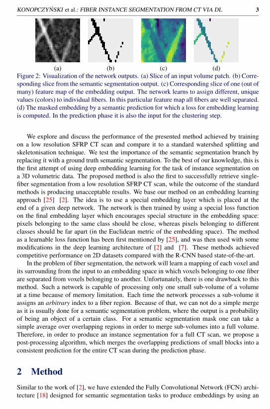
Figure 4: The input volume is represented by a number of embedded volumes at the em-bedding branch output. Here, slices of the first 12 embedding volumes corresponding to theinput sub-volume slice are visualized. Note, that a good embedding will assign different setof colors in each embedding volume so that the clustering in the embedding space will beeasy.

LCE , as is common for semantic segmentation tasks. It is defined as:

LCE =−[y · log(y)+(1− y) · log(1− y)] (1)

where y are the true binary labels, and y are the predicted labels. During the prediction phase,the output is thresholded at value 0.5 in order to produce binary masks. An example slice ofan output of the branch is shown in Fig 2 (b).

2.2 Embedding Learning Loss

The output of the embedding branch is a representation of the sub-volume in an embeddingspace. The architecture of the branch is identical to the semantic segmentation branch. Theonly difference is the number of output channels in the final convolutional layer and theloss function. In the semantic segmentation task, the output is producing a volume withtwo channels, where one is reasoning on the foreground and the other on the background.In the embedding learning, the output has as many channels as the dimensionality of theembedding space (a hyperparameter in the algorithm). An example visualizing feature mapsof the embeddings is shown in Fig. 4.

The loss function penalizes voxels of different instances that are too close to each otherin the embedding space and encourages voxels of the same instance to be close. As a result,the network maps the voxels into the embedding space, such that voxels that belong to thesame fiber should be placed next to each other and form easily separable clusters.

We find that the loss function introduced by [2] inspired by work of [25] and extendedto 3D by us works best for our problem. Even though we have extended the problem to3D, and have used data that contains a high number of objects compared to common scene-understanding problems, the method does not seem to be affected by that. The loss consistsof three terms: Lv keeps voxels belonging to the same object close to each other, Ld whichforces a minimal distance between clusters of different objects, and Lr which regularizes the

6 KONOPCZYNSKI et al.: FIBER INSTANCE SEGMENTATION FROM CT VIA DL

(a) (b) (c) (d)

Figure 5: 1. Visualization of the clustering steps of the method. (a) Masked embeddingsform clusters in a multi-dimensional embedding space (visualized by t-SNE). (b) DBSCANclusters the embedding representation and assign a different index (color) to each fiber (clus-ter) with black crosses for outliers. (c) Clusters are then mapped back to the spatial domain.Here a corresponding example slice of the mapping with red pixels for outliers. (d) Thewatershed algorithm is then applied as a post-processing step to fill the outliers.

cluster centers to be close to the origin. The terms are defined as:

Lv =1C

C

∑c=1

1Nc

Nc

∑i=1

[||µc− xi||−δv]2+ (2)

Ld =1

C(C−1)

C

∑cA=1

C

∑cB=1,cA 6=cB

[δd−||µcA −µcB ||]2+ (3)

Lr =1C

C

∑c=1||µc|| (4)

where C is the number of objects in the ground truth patch (clusters), Nc is the number ofvoxels that corresponds to the object c, xi is the embedding in the final embedding layer, µcis the mean of the embedding of object c, || · || is the L2 norm, and [x]+ = max(0,x). Theparameters δv and δd are used to control the desired positions of the clusters. The final lossfor the embedding learning Lembd is a sum of the previous components.

Lembd = αLv +βLd + γLr (5)

where α,β and γ control the strength of the corresponding term. An example slice of anoutput of the branch is visualized in Fig 2 (c). Note, that the loss is computed only based onthe voxels that belong to the foreground fibers. It is the task of the semantic segmentationbranch to find the correct position of the fibers.

2.3 ClusteringAs discussed in the previous section, the semantic segmentation output creates a confidencemap that a given voxel belongs to any fiber or not. A clustering is then applied to the em-bedded voxels with a high confidence of being fibers. An example input slice of one of thefeature maps of the embedding is shown in Fig 2 (d). In this work, we found DBSCAN [5]to work best on the SFRP dataset. In contrast to Mean Shift used in [2], DBSCAN does notmake assumptions about the shape of the clusters. We apply clustering only in the prediction

KONOPCZYNSKI et al.: FIBER INSTANCE SEGMENTATION FROM CT VIA DL 7

phase because the instance segmentation loss function does not require the instance segmen-tation map. Note, that DBSCAN does not necessarily assign a label to all voxels. Voxelsthat were not assigned to any label are assigned as outliers. The clusters are then mappedback to the spatial domain creating an instance segmentation map. Outliers are extrapolatedbased on their neighborhood in the spatial domain by use of the watershed algorithm, usingthe clustering labels as seeds. An example visualization of the described steps with help ofthe t-SNE [19] is shown in Fig 5.

2.4 Merging

Finally, the inference is produced on small overlapping sub-volumes of the entire volume.Each sub-volume contains different label IDs for fibers, making it not clear which fiber iswhich. To overcome this problem we have designed a merging algorithm, which joins labelIDs among the sub-volumes based on a spatial distance of fibers in the overlapped regions.The algorithm is applied at each sub-volume and processes recursively one fiber at a time,looking at neighboring sub-volumes with overlapping regions with objects being close to thefiber of interest. The merging procedure is described in more details in algorithm 1.

Algorithm 1 Merging algorithm1: procedure MERGE( f , p) . for a fiber f in a sub-volume p2: N← neighbour sub-volume of p . N is a set of sub-volumes neighbouring with p3: for sub-volume n in N do4: G← fibers in n . G is a set of fibers in a patch n5: for fiber g in G do6: d← D( f ,g) . Spatial distance between f and g7: if d > α then8: gid ← fid9: MERGE(g,n)

3 Experiments

3.1 Data

We have evaluated the proposed setup on two hand-annotated regions of low resolution CTscans of SFRP composites acquired by a Nikon MCT225 X-ray CT system from [15]. Scansexhibit typical artifacts and have low, but isotropic resolution. The parts from which thescans were acquired were manufactured by micro injection molding using PBT-10% GF,a commercial polybutylene terephthalate PBT (BASF, Ultradur B4300 G2) reinforced withshort glass fibers (10% in weight). The volumes have been hand annotated with center linesand processed by a watershed algorithm to create the instance segmentation ground truth.Both volumes are cubes of dimension 62 × 260 × 260 with approx. 6,500 fibers each.Fibers have a diameter of 10-14 µm (2-3 voxels) and are approx. 1.1 mm long. One scan isused for training, while the other is only used for testing.

8 KONOPCZYNSKI et al.: FIBER INSTANCE SEGMENTATION FROM CT VIA DL

Raw volume Ground truth CC Our method

Figure 6: Visualization of the testing volume and corresponding results. First row shows a3D rendering of a volume. Second row shows one example slice of the same volume. Firstcolumn is the input test volume (with a certain threshold to remove the epoxy background inthe 3D rendering). Second column is the corresponding ground truth. Third column is theoutput of a standard connected component (CC) analysis. Fourth column is the output of ourmethod. Fibers are colored semi-randomly based on the fiber ID.

3.2 Training details

The volumes have been normalized to have unit variance and zero mean. Additionally, mostof the air voxels surrounding the specimen have been removed by a simple thresholdingmethod. We have trained and evaluated the network on sub-volumes of 32× 32× 32 fromthe training volume. The sub-volumes are randomly flipped and rotated (by 90, 180 or 270degrees) during the training phase. As mentioned in the introduction, and shown in Figure3, for backbones of both the semantic segmentation and embedding learning branch we haveused the architecture proposed in [16] designed for semantic fiber segmentation. It is a 3DFCN with standard residual units [10] and batch normalization [13] but with no max-poolingto keep the resolution of the already very thin fibers.

The embedding learning is not stable, when trained from noise. Therefore, first we havetrained the semantic segmentation branch for 20,000 iterations and saved the weights. Then,we have used the weights as an initialization for the embedding learning branch and trainedit for another 20,000 iterations. The loss used for training the embedding learning uses thesemantic ground truth masks.

It would also have been an option to share the embeddings and weights for both tasks.Such setup is reported to slightly increase the performance of both semantic and instance seg-mentation [20]. However, in our setup, we have found the above two-stage training to workbetter. We use 16 feature embedding maps and set α and β to 1 and γ to 0.001. Optimizationhas been done by using the Adam optimizer [14] with an initial learning rate set to 0.001.During the prediction phase, the algorithm processes overlapping 32×32×32 sub-volumesof the test volume with an overlap of 16 in each direction. The post-processing mergingalgorithm merges the overlapping sub-volumes and produces the final instance segmentationvolume.

KONOPCZYNSKI et al.: FIBER INSTANCE SEGMENTATION FROM CT VIA DL 9

Setup Mean ARI Merged ARIEmbedding Learning 0.9048 0.6529

Embedding Learning + true semantic 0.9129 0.7817Connected Components 0.3537 0.2112

Connected Components + true semantic 0.3614 0.2534

Table 1: Comparison of our method with traditional connected components with and with-out provided ground truth semantic segmentation mask. Mean ARI are mean values overoverlapping sub-volumes of the validation volume, while Merged ARI is the score computedover the entire volume after the post-processing merging step. The Dice score of the semanticsegmentation mask from the semantic segmentation branch is 0.9784.

For a metric we have use the Adjusted Rand Index [12] to measure the performance ofinstance segmentation. We find it more informative in the context of SFRP data over themAP. Defining the ground truth labels as clusters C = {C1, ...,Ck} and the correspondingpredicted labels as clusters C = {C1, ...,Cl}, the Adjusted Rand Index Ra is:

Ra(C,C) =∑

ki=1 ∑

lj=1

(mi j2

)− t3

12 (t1 + t2)− t3

(6)

where mi j = |Ci∩C j|, t1 = ∑ki=1

(|Ci|2

), t2 = ∑

lj=1

(|C j |2

), t3 =

2t1t2n(n−1) , and n is the number

of voxels in the volume. The Rand Index varies from 0 to 1, where 1 means a perfect matchbetween the algorithm output and the ground truth mask.

3.3 Results

We have compared our method to a standard skeletonization followed by connected com-ponent analysis and the Watershed method [26]. In the method, a binary erosion is firstapplied on the semantic mask, which serves as seeds after connected component analysisfor a watershed segmentation algorithm. See Fig. 6 for a visual comparison. We have alsoevaluated the importance of a good semantic segmentation mask. We provide results forboth our method and connected components given the semantic segmentation computed bythe semantic segmentation branch as well as using the ground truth semantic segmentation.

Therefore we compare four different setups. Our Embedding Learning method using thefinal instance segmentation produced given the semantic segmentation mask from the se-mantic segmentation branch. Embedding Learning + true semantic which is our method butusing ground truth semantic segmentation mask instead of the one produced by the meth-ods branch (which is not ideal). Connected Components and Connected Components + truesemantic is the connected component method used either on the output of the semantic seg-mentation branch or the ground truth semantic mask.

We provide two results in Table 1 for each setup. In the first column, the mean ARI is themean ARI of all the sub-volumes in the test volume without the merging step. In the secondcolumn one can see the score computed over the entire volume after the post-processingmerging step which we call a merged ARI. We report the ARI score only for the voxels thatbelong to the ground truth instance segmentation mask. Including the background voxelswould artificially increase the score.

10 KONOPCZYNSKI et al.: FIBER INSTANCE SEGMENTATION FROM CT VIA DL

While the standard method clearly fails even when using the true semantic segmentationmask, the proposed method produces meaningful results in all cases. When reasoning onsmall overlapping patches the proposed method achieves 0.9048 average ARI score. Themerging algorithm has trouble with ambiguity of two neighboring outputs and favors merg-ing over splitting. This results in merging two fibers into one, when they are too close toeach other. After the merging post-processing step the ARI score decreases to 0.6529.

4 ConclusionsIn this work, we proposed a deep 3D fully convolutional architecture together with a set ofpost-processing steps for a problem of single fiber segmentation from CT scans of SFRP. Weextend a less common approach of embedding learning for the task of 3D instance segmen-tation. We explain in detail the steps of the method together with a post-processing and amerging procedure. We show that we are better than the traditional skeletonization - water-shed method. We expect our findings to be applicable to a wide variety of volumetric dataand not only to fiber composites.

References[1] M. Bai and R. Urtasun. Deep watershed transform for instance segmentation. Confer-

ence on Computer Vision and Pattern Recognition, pages 2858–2866, 2017.

[2] B. De Brabandere, D. Neven, and L. Van Gool. Semantic instance segmentation with adiscriminative loss function. arXiv preprint arXiv:1708.02551., 2017.

[3] P. F. Christ, M. E. A. Elshaer, F. Ettlinger, S. Tatavarty, M. Bickel, P. Bilic, and W. H.Sommer. Automatic liver and lesion segmentation in ct using cascaded fully convolu-tional neural networks and 3d conditional random fields. International Conference onMedical Image Computing and Computer-Assisted Intervention, pages 415–423, 2016.

[4] J. Deng, W. Dong, R. Socher, L. J. Li, K. Li, and L. Fei-Fei. Imagenet: A large-scalehierarchical image database. Conference on Computer Vision and Pattern Recognition,pages 248–255, 2009.

[5] M. Ester, H. P. Kriegel, J. Sander, and X. Xu. Density-based spatial clustering ofapplications with noise. Int. Conf. Knowledge Discovery and Data Mining, 1996.

[6] T. Fast, A. E. Scott, H. A. Bale, and B. N. Cox. Topological and euclidean metricsreveal spatially nonuniform structure in the entanglement of stochastic fiber bundles.Journal of materials science, 50(6):2370–2398, 2015.

[7] A. Fathi, Z. Wojna, V. Rathod, P. Wang, H. O. Song, S. Guadarrama, and K. P.Murphy. Semantic instance segmentation via deep metric learning. arXiv preprintarXiv:1703.10277., 2017.

[8] A. F. Frangi, W. J. Niessen, K. L. Vincken, and M. A. Viergever. Multiscale vesselenhancement filtering. In International Conference on Medical Image Computing andComputer-Assisted Intervention, 1998.

KONOPCZYNSKI et al.: FIBER INSTANCE SEGMENTATION FROM CT VIA DL 11

[9] S. Y. Fu and B. Lauke. Effects of fiber length and fiber orientation distributions on thetensile strength of short-fiber-reinforced polymers. Composites Science and Technol-ogy, 56(10):1179–1190, 1996.

[10] K. He, X. Zhang, S. Ren, and J. Sun. Deep residual learning for image recognition.Conference on Computer Vision and Pattern Recognition, pages 770–778, 2016.

[11] K. He, G. Gkioxari, P. Dollár, and R. Girshick. Mask r-cnn. International Conferenceon Computer Vision, pages 2980–2988, 2017.

[12] L. Hubert and P. Arabie. Comparing partitions. Journal of classification, 2(1):193–218,1985.

[13] S. Ioffe and C. Szegedy. Batch normalization: Accelerating deep network training byreducing internal covariate shift. arXiv preprint arXiv:1502.03167, 2015.

[14] D. P. Kingma and J. Ba. Adam: A method for stochastic optimization. arXiv preprintarXiv:1412.6980, 2014.

[15] T. Konopczynski, J. Rathore, T. Kröger, L. Zheng, C. S. Garbe, S. Carmignato, andJ. Hesser. Reference setup for quantitative comparison of segmentation techniques forshort glass fiber ct data. Conference on Industrial Computed Tomography, 2017.

[16] T. Konopczynski, D. Rathore, J. Rathore, T. Kröger, L. Zheng, C. S. Garbe,S. Carmignato, and J. Hesser. Fully convolutional deep network architectures for auto-matic short glass fiber semantic segmentation from ct scans. Conference on IndustrialComputed Tomography, 2018.

[17] T. Y. Lin, M. Maire, S. Belongie, J. Hays, P. Perona, D. Ramanan, and C. L. Zitnick.Microsoft coco: Common objects in context. European conference on computer vision,pages 740–755, 2014.

[18] J. Long, E. Shelhamer, and T. Darrell. Fully convolutional networks for semantic seg-mentation. conference on computer vision and pattern recognition, pages 3431–3440,2015.

[19] L. V. D. Maaten and G. Hinton. Visualizing data using t-sne. Journal of machinelearning research, 9:2579–2605, 2008.

[20] D. Neven, B. De Brabandere, S. Georgoulis, M. Proesmans, and L. Van Gool. Fastscene understanding for autonomous driving. arXiv preprint arXiv:1708.02550, 2017.

[21] P. Pinter, B. Bertram, and K. A. Weidenmann. A novel method for the determination offibre length distributions from uct-data. Conference on Industrial Computed Tomogra-phy, 2016.

[22] S. Ren, K. He, R. Girshick, and J. Sun. Faster r-cnn: Towards real-time object detectionwith region proposal networks. Advances in neural information processing systems,pages 91–99, 2015.

[23] B. Romera-Paredes and P. H. S. Torr. Recurrent instance segmentation. EuropeanConference on Computer Vision, pages 312–329, 2016.

12 KONOPCZYNSKI et al.: FIBER INSTANCE SEGMENTATION FROM CT VIA DL

[24] R. M. Sencu, Z. Yang, Y. C. Wang, P. J. Withers, C. Rau, A. Parson, and C. Soutis.Generation of micro-scale finite element models from synchrotron x-ray ct images formultidirectional carbon fibre reinforced composites. Composites Part A: Applied Sci-ence and Manufacturing, 91:85–95, 2016.

[25] K. Q. Weinberger and L. K. Saul. Distance metric learning for large margin nearestneighbor classification. Journal of Machine Learning Research, 10:207–244, 2009.

[26] X. Zhang, D. Li, W. Yang, J. Wang, and S. Liu. A fast segmentation method for high-resolution color images of foreign fibers in cotton. Composites Part A: Applied Scienceand Manufacturing, 78(1):71–79, 2011.