Deep Instance Segmentation with Automotive Radar ... - OSF

1

Deep Instance Segmentation with Automotive RadarDetection Points

Jianan Liu∗, Weiyi Xiong∗, Liping Bai, Yuxuan Xia, Tao Huang, Wanli Ouyang, Bing Zhu†

Abstract—Automotive radar provides reliable environmentalperception in all-weather conditions with affordable cost, butit hardly supplies semantic and geometry information due tothe sparsity of radar detection points. With the developmentof automotive radar technologies in recent years, instance seg-mentation becomes possible by using automotive radar. Its datacontain contexts such as radar cross section and micro-Dopplereffects, and sometimes can provide detection when the fieldof view is obscured. The outcome from instance segmentationcould be potentially used as the input of trackers for track-ing targets. The existing methods often utilize a clustering-based classification framework, which fits the need of real-time processing but has limited performance due to minimuminformation provided by sparse radar detection points. In thispaper, we propose an efficient method based on clustering ofestimated semantic information to achieve instance segmentationfor the sparse radar detection points. In addition, we showthat the performance of the proposed approach can be furtherenhanced by incorporating the visual multi-layer perceptron. Theeffectiveness of the proposed method is verified by experimentalresults on the popular RadarScenes dataset, achieving 89.53%mCov and 86.97% mAP0.5, which is the best comparing to otherapproaches in the literature. More significantly, the proposedalgorithm consumes memory around 1MB, and the inferencetime is less than 40ms. These two criteria ensure the practicalityof the proposed method in real-world systems.

Index Terms—Autonomous driving, environmental perception,instance segmentation, semantic segmentation, clustering, classi-fication, automotive radar, deep learning

I. INTRODUCTION

IN the field of autonomous driving, automotive radar playsan important role in environmental perception due to its

affordable cost, inherent measurement of object relative ve-locity, and reliability in all-weather conditions, as comparedto camera and LiDAR [2][3]. The data representation of anautomotive radar is usually a set of sparse detection pointsgenerated by pre-processed raw radar signals typically in theform of a range-Doppler map or a range-azimuth heatmap.

J. Liu is with Vitalent Consulting, Gothenburg 41761, Sweden, and SiloAI, Stockholm, Sweden. Email: [email protected], [email protected]

W. Xiong, L. Bai and B. Zhu are with School of Automation Scienceand Electrical Engineering, Beihang University, Beijing 100191, P.R. China.Email: [email protected] (W.Xiong); bai [email protected] (L.Bai);[email protected] (B.Zhu)

Y. Xia is with Department of Electrical Engineering, Chalmers Universityof Technology, Gothenburg 41296, Sweden. Email: [email protected]

T. Huang is with College of Science and Engineering, James CookUniversity, Cairns, Australia. Email: [email protected]

W. Ouyang is with SIGMA Lab, School of Electrical and Informa-tion Engineering, The University of Sydney, Sydney, Australia. Email:[email protected]

∗Both authors contribute equally to the work and are co-first authors.†Corresponding author.

Motorbike

Car

Pedestrian

Car

Car

Car

(a) City Drive

Truck

Car

Car

Car

Car

Car

Car

Car

Car

(b) Federal Highway Ramp

Car

Car

Other

Car

Car

Ped. Group

Car

Car

Car

Car

Motorbike

(c) Crowded Street

Car

Car

Car

(d) Intersection – Rainy Day

Car

Car

Car

Car

(e) Transvision Effect

Car

Car

(f) Tunnel

Car

Truck

Car

(g) Unrealistic Proportions

Ped. Group

Ped. Group

Ped. Group

(h) Pedestrian Group

Ped. Group

Car

Car

Bicycle

Car

Car

Car

(i) Inner City

Car

Pedestrian

Car

Car

Pedestrian

Other

Car

Bicycle

CarBicycle

Pedestrian

Bicycle

Pedestrian

Bicycle

(j) Inner City Intersection – Full Field of View

Fig. 2: Radar bird’s-eye view point cloud images and corresponding camera images. Orientation and magnitude of each point’sestimated radial velocity after ego-velocity compensation are depicted by gray arrows. In the documentation camera images,road users are masked due to EU regulations (GDPR). Images allow for intensive zooming.

balanced label distribution is required to achieve good perfor-mance, e.g., for classification or object detection tasks, e.g.,[3], [9]. For this mapping, the animal and the other classare not reassigned. Instead they may be used, e.g., for a hiddenclass detection task, cf. [4].

Two labels are assigned to each individual detection of adynamic object: a label id and a track id. The labelid is an integer describing the semantic class the respectiveobject belongs to. On the other hand, the track id identifiessingle real world objects uniquely over the whole recording

(a) Radar Detection Points

Motorbike

Car

Pedestrian

Car

Car

Car

(a) City Drive

Truck

Car

Car

Car

Car

Car

Car

Car

Car

(b) Federal Highway Ramp

Car

Car

Other

Car

Car

Ped. Group

Car

Car

Car

Car

Motorbike

(c) Crowded Street

Car

Car

Car

(d) Intersection – Rainy Day

Car

Car

Car

Car

(e) Transvision Effect

Car

Car

(f) Tunnel

Car

Truck

Car

(g) Unrealistic Proportions

Ped. Group

Ped. Group

Ped. Group

(h) Pedestrian Group

Ped. Group

Car

Car

Bicycle

Car

Car

Car

(i) Inner City

Car

Pedestrian

Car

Car

Pedestrian

Other

Car

Bicycle

CarBicycle

Pedestrian

Bicycle

Pedestrian

Bicycle

(j) Inner City Intersection – Full Field of View

Fig. 2: Radar bird’s-eye view point cloud images and corresponding camera images. Orientation and magnitude of each point’sestimated radial velocity after ego-velocity compensation are depicted by gray arrows. In the documentation camera images,road users are masked due to EU regulations (GDPR). Images allow for intensive zooming.

balanced label distribution is required to achieve good perfor-mance, e.g., for classification or object detection tasks, e.g.,[3], [9]. For this mapping, the animal and the other classare not reassigned. Instead they may be used, e.g., for a hiddenclass detection task, cf. [4].

Two labels are assigned to each individual detection of adynamic object: a label id and a track id. The labelid is an integer describing the semantic class the respectiveobject belongs to. On the other hand, the track id identifiessingle real world objects uniquely over the whole recording

(b) Image

Fig. 1. An example frame of (a) bird eye’s view radar detection point cloudimage and (b) its corresponding image in RadarScenes dataset [1] ©IEEE.The measurements were collected via 77 GHz series production automotiveradar sensors.

Compared to LiDAR points, radar detection points usuallyprovide more information, e.g., velocity (Doppler) and theradar cross section (RCS) values. However, radar detectionpoints are much sparser and nosier than LiDAR point cloudsdue to their low resolution, resulting in a lack of semanticand geometric information. Fig. 1 shows a typical scene inRadarScenes dataset [1] including the collected data from bothradar and camera. Note that the collected radar detection pointsare sparse and semantically ambiguous. Thus, it is unsuitableto directly apply methods developed for dense LiDAR pointclouds to sparse radar detection points.

There are three popular methods in the literature to per-form point cloud instance segmentation [4]. The first methodtransforms a point cloud into a 3D grid-like representationcalled voxel, or projects it into a 2D grid-like representationlike the bird eye’s view (BEV) or a range view, and usesa convolutional neural network (CNN) to segment instance.The drawback of this method is that it requires a largememory, high computation power, and introduces quantizationerror in the point-to-voxel/pixel transformation. The secondmethod directly processes the points using a 1D convolutionalfilter-based neural network, treating spatial coordinates aspart of the features. Typical examples include the PointNets[5][6] and their variants [7][8]. This method could overcomethe quantization error encountered by the first method andpotentially directly extracts more fruitful feature informationfrom dense points. However, the encoders of neural networksin both first and second methods have difficulty capturingthe spatial interactions of radar detection points due to theirsparsity [9]. The third method is to estimate which pointsbelong to the same object using a clustering algorithm, e.g. theDensity-Based Spatial Clustering of Applications with Noise(DBSCAN) [10], and then perform the classification for each

2

estimated cluster. Although the performance of this methodis limited compared to the deep learning-based methods,it still dominates the radar-based instance segmentation inpractice due to its simplicity [11][12][13], which minimizesthe memory consumption and favors real-time data processing.

In this paper, we propose a new strategy and its enhance-ment version for instance segmentation on automotive radardetection points to combat issues in the aforementioned meth-ods. Our goal is to develop a new and practical deep-learningarchitecture that can handle the sparse radar detection pointsfor segmentation process with small memory requirementand fast run time. The main contributions of this paper aresummarized as follows:

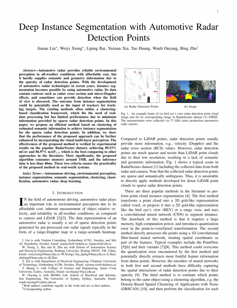
• We design a novel semantic segmentation-based cluster-ing method for the instance segmentation task on sparsepoint clouds obtained from automotive radar. The modelis designed base on the semantic segmentation versionof PointNet++ [6], with a newly introduced head thatestimates the point-wise center shift vector (CSV) whichrepresents the offset in latent space from every detec-tion point to the geometric center of its correspondinginstance. By shifting each point toward the center of itsinstance with predicted CSV during clustering, the pointsbelonging to the same instance become closer, whichincrease the clustering accuracy.

• We propose to use cosine similarity (CS) loss and nor-malized inner product (NIP) loss in the training processof the semantic segmentation phase for sparse radardetection points, to improve the performance of CSVguided clustering. These loss functions are designed tominimize the distance between the predicted and ground-truth CSV in latent space, resulting in more accurateprediction of CSVs.

• We investigate how various visual multi-layer perceptrons(MLPs) [14][15][16] can be incorporated to the proposedmethod, and propose to employ gMLP to further improvethe performance of our model. A thorough search of theliterature yielded no existing study on adopting visualMLPs in radar sensing to overcome the limitation of localfeature extraction due to the sparsity of radar detectionpoints. In addition, we propose tailored lightweight meth-ods to achieve a balance among the computation speed,memory consumption and accuracy.

• We experiment with the proposed method on the recentRadarScenes dataset [1] and demonstrate that the per-formance of the proposed method outperforms the twoexisting methods by a large margin. Precisely, the meancoverage (mCov) and the mean average precision (mAP)of our selected method are 9.0% and 9.2% higher thanthe clustering-based classification method, and 8.6% and9.1% higher than the end-to-end instance segmentationmethod, respectively. At the same time, our methodand its lightweight version still maintain the memoryconsumption around 1MB and inference time less than40ms, which are feasible for automotive radar micro-center unit (MCU). Such an outcome reveals the potentialto apply our proposed strategy in the real-time automotive

radar perception system.The rest of this paper is organized as follows. Section

II discusses the related works, including point cloud pro-cessing methods, visual MLPs, and radar-based perception.The proposed radar-based instance segmentation method andits enhancements are described in Section III. Section IVdescribes the experiment process and presents the results onthe RadarScenes dataset. Discussions are also made in thissection. Finally, concluding remarks are drawn in section V.

II. RELATED WORKS

There are three main considerations in this work: pointcloud processing, visual MLPs and automotive radar-basedperception. We will discuss each of them in this section.

A. Point Cloud Processing

Point clouds are sporadic and permutation invariant, makingeffective information extraction challenging. While the imageprocessing techniques, such as 2D convolution, can be extrap-olated into the realm of 3D point cloud data processing, theoutcomes of such approaches turn out to be ineffective.

PointNet [5] and the subsequent variants [6] are networkstructures designed specifically for point cloud data, where theinput data points are projected into a higher dimension spacebefore going through a permutation invariant function, e.g., amax pooling function, for feature extraction. As opposed toPointNet that taking all the data points as the input of the firstlayer, PointNet++ [6] seeks to imitate the convolution layer of2D images and attempt to capture the local context. To achievethis, a set abstraction (SA) layer is used to sample, grouppoints and capture local structure. Furthermore, the featurepropagation (FP) layer is devised to propagate features fromsampled points to original points and get point-wise features,for the purpose of segmentation.

PointNet and PointNet++ do not provide the function ofdirect instance segmentation, but some efforts have beenmade toward this direction. For instance, SGPN [7] takesPointNets as its backbone and introduce a similarity matrixfor instance segmentation. HAIS [8] combines PointNets withclustering, adopts hierarchical aggregation to progressivelygenerate instance proposals.

B. Visual MLPs

Attention-based transformers [17][18][19] are popular ap-proaches for computer vision tasks, but some recent worksprove that comparable performance can be achieved by usingMLPs only. MLP-mixer [15] replaces the the multi-head selfattention [20] with a linear layer implemented on the spatialdimension. To make the MLP flexible to receive images ofdifferent sizes, researchers propose cycle-MLP [21], where acycle fully connected (FC) layer is used to replace the spatialMLP in MLP-mixer [15]. However, as the data structure ofimages and point clouds are different, such method cannot beapplied to our work without voxelizing the point cloud. gMLP[16] discards the multi-head self attention in transformer andadd a spatial gating unit to capture spatial interaction. Taking

3

Clustering

(DBSCAN)

Original Detection Points Predicted Instance Segmentation Results

C

N

Feature Map(Point-wise Features)

MLP

MLP

Poin

tNet

++ /

Visu

al M

LP

Enha

nced

Poi

ntN

et++

ndim

N

Point-wise Predicted Center Shift Vectors

Softmax

nclass

N

Semantic Matrix(Point-wise Per-class Scores)

MAX

Point-wise Predicted Class

N

1

Points Shifting Using

Center Shift Vectors

Point-wise Classification Branch(Semantic Segmentation Branch)

CSVs Prediction Branch

N:C:

nclass:ndim:

Sample SizeThe Number of Output ChannelsThe Number of ClassesThe Dimension of Raw Radar Detection Points

B Batch size

N Sample size

C # output channels

nclass # classes

ndim The dimension of raw radar detection points

B:N:C:

nclass:ndim:

Batch SizeSample SizeThe Number of Output ChannelsThe Number of ClassesThe Dimension of Raw Radar Detection Points

N:C:

nclass:ngroup:

Sample SizeThe Number of Output ChannelsThe Number of ClassesThe Number of Predicted Groups

Fig. 2. Illustration for the entire process of our proposed semantic segmentation-based clustering. N denotes the sample size, and C represents the numberof output channels of the backbone; nclass is the number of classes and ndim denotes the dimension of raw radar detection points. The input points obtaintheir predicted class label through the point-wise classification branch firstly. Then they are shifted according to their predicted CSVs which are estimated bythe CSVs prediction branch, so that the points belonging to the same instance are more concentrated. Points with the same class label are then clustered intoclusters (i.e., instances). In the instance segmentation results of the example frame, different colors denote different classes, where points in the same circlebelong to the same instance.

the inspiration from self-attention, external attention [14] usestwo linear layers with a double normalization in between, toreduce the computational complexity.

C. Automotive Radar-based Perception

Automotive radar-based perception, including semantic seg-mentation, clustering, classification, instance segmentation,object detection, and tracking, has played an essential role inthe modern ADAS and autonomous driving system. With theavailability of large-scale radar datasets [1], automotive radardetection points-based perception has been investigated re-cently [11][12][22][23][24]. A two-stage clustering algorithmis designed in [22]. Moreover, estimated state informationusing an extended target tracking algorithm is employed in[25] as prior information to provide more stable clustering.Conventional machine learning and modern deep learningmethods have also been explored for automotive radar detec-tion points-based perception. For example, the radar detectionpoints are used as input data for semantic segmentation task[23], together with occupancy grid representation of environ-ments [26][27]. Such detection points representation of radardata is also employed for classification, object detection andtracking purpose. For example, [11][12][28] utilize randomforest and LSTM to classify clustered detection points, [9]modifies the PointNets for object detection but only one class(cars) are considered, and [24] performs detection and trackingby adopting the combination of PointNet++ based neuralnetwork with a Kalman filter and global nearest neighbor forID assignment over multiple frames.

III. PROPOSED METHODS

In this section, we first introduce the proposed semanticsegmentation-based clustering strategy. Then, we present itsenhanced version with visual MLPs.

A. Semantic Segmentation-based Clustering

Dense points, such as LiDAR point cloud, on one hand hasrich geometric and semantic information. On the other hand,GPUs are usually available to support processing of massivenumber of points in LiDAR point cloud, so that large modelscould be designed and high computational algorithms could bedeveloped. In contrast, sparse radar detection points which aresemantically ambiguous, cannot reflect the shape of objects.In addition, only MCU with low computational capabilityand small memory space could be available to process radardetection points in real time, in the typical low cost automotiveradar system. As a result, the existing end-to-end instancesegmentation methods designed for dense point clouds [7] arenot suitable for sparse radar detection points.

In this work, we propose an instance segmentation methodfor radar detection points, which is semantic segmentation(point-wise classification) based clustering. Specifically, wefirst let the network model concentrate on semantic segmen-tation. Then we apply a clustering method for each class ofdetection points, since detection points assigned with differentsemantic information can scarcely belong to the same instance.

Moreover, it is intuitive that clustering different classes ofpoints with different clustering parameter settings may achievebetter performance, because the attributes of clusters belongto various class types might be significantly different. Forinstance, there may be more than 10 detection points froma large vehicle, and the distances between these detectionpoints could be larger than those from a two-wheeler, while apedestrian may only have one detection point. Thus, differentclustering parameter settings can be used for different classes.

Our proposed semantic segmentation-based clusteringmethod is illustrated in Fig. 2, where we adopt the PointNet++based network to perform semantic segmentation, and wechoose DBSCAN as our clustering method. Concretely, theinput point cloud is first processed by a PointNet++ basedfeature extractor to generate a feature map, and then point-wise features are sent to the point-wise classification branch to

4

B C

N

B ndim

N

Predicted Center Shift Vectors

Softmax

B nclass

N

Semantic Matrix(Point-wise Per-class Scores)

Set A

bstra

ctio

n

Set A

bstra

ctio

n

Feat

ure

Prop

agat

ion

Feat

ure

Prop

agat

ion

Visu

al M

LP B

lock

Visu

al M

LP B

lock

Visu

al M

LP B

lock

Visu

al M

LP B

lock

Skip Connection

Set A

bstra

ctio

n

Set A

bstra

ctio

n

Feat

ure

Prop

agat

ion

Feat

ure

Prop

agat

ion

Skip Connection

Skip Connection

Skip Connection

A Batch of Framesof Radar

Detection Points

A Batch of Framesof Radar

Detection Points

B

B

LSEM

The Center of the InstanceThe Predicted Center Shift VectorThe Ground-truth Center Shift Vector

LSHIFT

L

(a) (b)

(d) (c)

B

N

1

Ground-truth Point-wise ClassFeature Map

(Point-wise Features)

1×1

Con

v

1×1

Con

v

Bat

chN

orm

ReL

U

Dro

pout

1×1

Con

v

1×1

Con

v

Bat

chN

orm

ReL

U

Dro

pout

Interchangeable

B C

N

Feature Map(Point-wise Features)

Enhanced Design

B

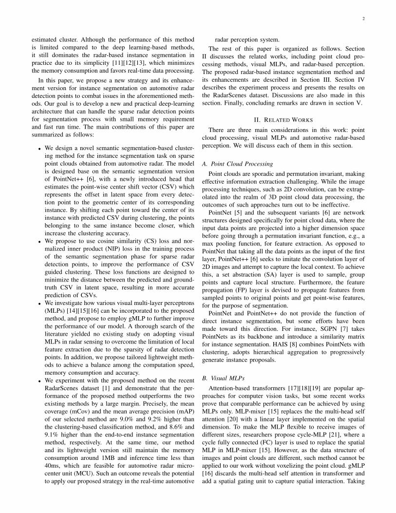
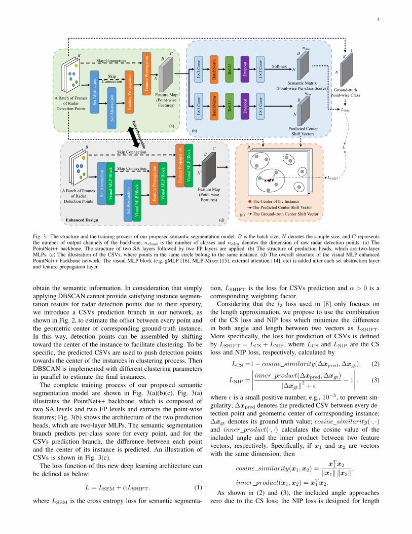
Fig. 3. The structure and the training process of our proposed semantic segmentation model. B is the batch size, N denotes the sample size, and C representsthe number of output channels of the backbone; nclass is the number of classes and ndim denotes the dimension of raw radar detection points. (a) ThePointNet++ backbone. The structure of two SA layers followed by two FP layers are applied. (b) The structure of prediction heads, which are two-layerMLPs. (c) The illustration of the CSVs, where points in the same circle belong to the same instance. (d) The overall structure of the visual MLP enhancedPointNet++ backbone network. The visual MLP block (e.g. gMLP [16], MLP-Mixer [15], external attention [14], etc) is added after each set abstraction layerand feature propagation layer.

obtain the semantic information. In consideration that simplyapplying DBSCAN cannot provide satisfying instance segmen-tation results for radar detection points due to their sparsity,we introduce a CSVs prediction branch in our network, asshown in Fig. 2, to estimate the offset between every point andthe geometric center of corresponding ground-truth instance.In this way, detection points can be assembled by shiftingtoward the center of the instance to facilitate clustering. To bespecific, the predicted CSVs are used to push detection pointstowards the center of the instances in clustering process. ThenDBSCAN is implemented with different clustering parametersin parallel to estimate the final instances.

The complete training process of our proposed semanticsegmentation model are shown in Fig. 3(a)(b)(c). Fig. 3(a)illustrates the PointNet++ backbone, which is composed oftwo SA levels and two FP levels and extracts the point-wisefeatures; Fig. 3(b) shows the architecture of the two predictionheads, which are two-layer MLPs. The semantic segmentationbranch predicts per-class score for every point, and for theCSVs prediction branch, the difference between each pointand the center of its instance is predicted. An illustration ofCSVs is shown in Fig. 3(c).

The loss function of this new deep learning architecture canbe defined as below:

L = LSEM + αLSHIFT, (1)

where LSEM is the cross entropy loss for semantic segmenta-

tion, LSHIFT is the loss for CSVs prediction and α > 0 is acorresponding weighting factor.

Considering that the l2 loss used in [8] only focuses onthe length approximation, we propose to use the combinationof the CS loss and NIP loss which minimize the differencein both angle and length between two vectors as LSHIFT.More specifically, the loss for prediction of CSVs is definedby LSHIFT = LCS + LNIP, where LCS and LNIP are the CSloss and NIP loss, respectively, calculated by

LCS =1− cosine similarity(∆xpred,∆xgt), (2)

LNIP =

∣∣∣∣∣ inner product(∆xpred,∆xgt)

∥∆xgt∥2 + ϵ− 1

∣∣∣∣∣ , (3)

where ϵ is a small positive number, e.g., 10−5, to prevent sin-gularity; ∆xpred denotes the predicted CSV between every de-tection point and geometric center of corresponding instance;∆xgt denotes its ground truth value; cosine similarity(·, ·)and inner product(·, ·) calculates the cosine value of theincluded angle and the inner product between two featurevectors, respectively. Specifically, if x1 and x2 are vectorswith the same dimension, then

cosine similarity(x1,x2) =xT1 x2

∥x1∥ ∥x2∥,

inner product(x1,x2) = xT1 x2.

As shown in (2) and (3), the included angle approacheszero due to the CS loss; the NIP loss is designed for length

5

Inpu

t Fea

ture

s

Out

put F

eatu

res

Laye

rNor

m

Cha

nnel

Pro

j.

Cha

nnel

Pro

j.

GeL

U

Spat

ial P

roj.

Laye

rNor

m

Split+ •

Spatial Gating Unit

gMLP Block

Cha

nnel

=2C

i

Cha

nnel

=Ci

Cha

nnel

=Ci K

eep

Dim

Cha

nnel

=Ci

Cha

nnel

=Ci

Inpu

t Fea

ture

s

Out

put F

eatu

res

Laye

rNor

m

Cha

nnel

Pro

j.

Cha

nnel

Pro

j.

GeL

U

Spat

ial P

roj.

Laye

rNor

m

Split+ •

Spatial Gating Unit

gMLP Block

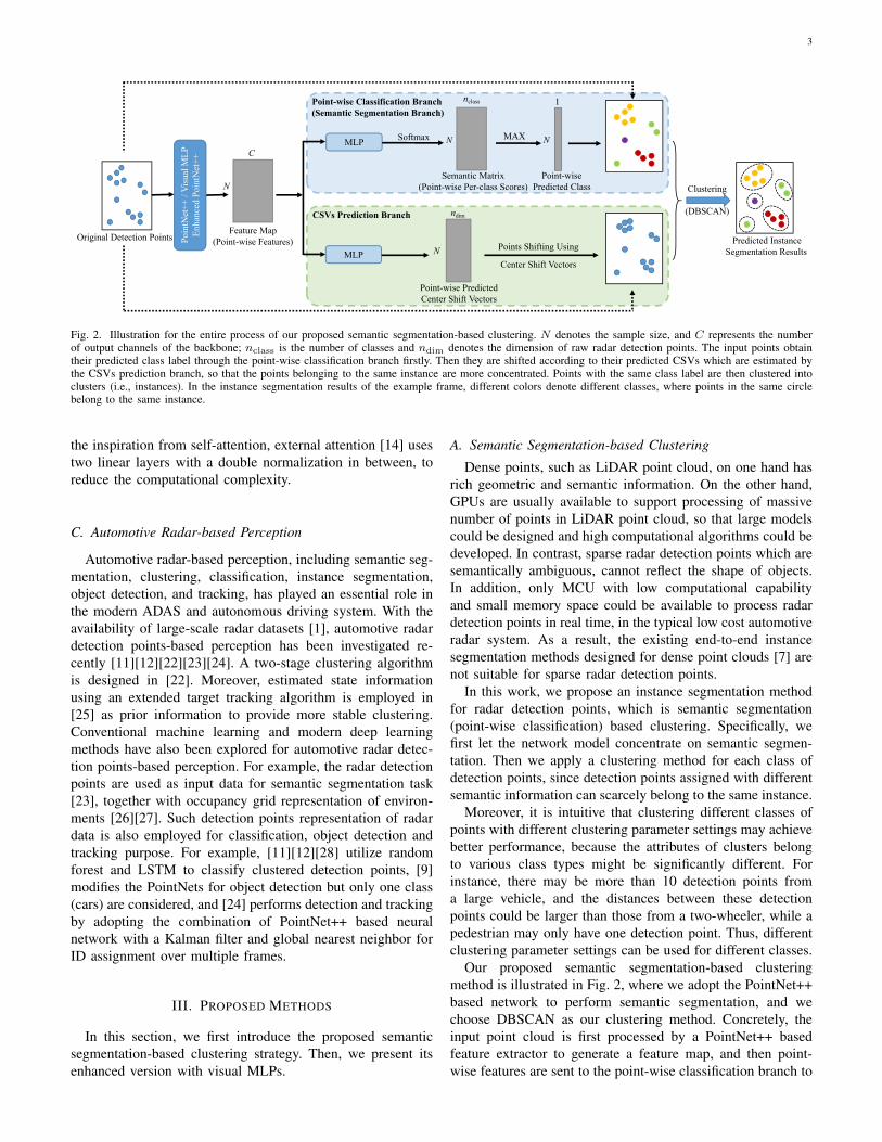
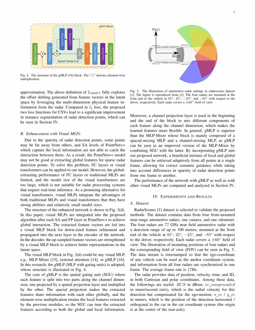
Fig. 4. The structure of the gMLP [16] block. The “⊙” denotes element-wisemultiplication.

approximation. The above definition of LSHIFT fully exploresthe offset shifting generated from feature vectors in the latentspace by leveraging the multi-dimension physical feature in-formation from the radar. Compared to l2 loss, the proposedtwo loss functions for CSVs lead to a significant improvementin instance segmentation of radar detection points, which canbe seen in Section IV.

B. Enhancement with Visual MLPs

Due to the sparsity of radar detection points, some pointsmay be far away from others, and SA levels of PointNet++which capture the local information are not able to catch theinteraction between them. As a result, the PointNet++ modelmay not be good at extracting global features for sparse radardetection points. To solve this problem, FC layers or visualtransformers can be applied to our model. However, the global-extracting performance of FC layers or traditional MLPs arelimited, and the model size of the visual transformers aretoo large, which is not suitable for radar processing systemsthat require real-time inference. As a promising alternative forvisual transformers, visual MLPs integrate the advantages ofboth traditional MLPs and visual transformers that they havestrong abilities and relatively small model sizes.

The structure of the enhanced network is shown in Fig. 3(d).In this paper, visual MLPs are integrated into the proposedalgorithm after each SA and FP layer in PointNet++ to achieveglobal interaction. The extracted feature vectors are fed intoa visual MLP block for down-sized feature refinement andpropagated into the next layer in the encoder of the network.In the decoder, the up-sampled feature vectors are strengthenedby a visual MLP block to achieve better representations in thelatent space.

The visual MLP block in Fig. 3(d) could be any visual MLP,e.g., MLP-Mixer [15], external attention [14], or gMLP [16].In this research, the gMLP (MLP with gating units) is adopted,whose structure is illustrated in Fig. 4.

The core of gMLP is the spatial gating unit (SGU) whereeach feature is split into two parts along the channel dimen-sion, one projected by a spatial projection layer and multipliedby the other. The spacial projection makes the extractedfeatures share information with each other globally, and theelement-wise multiplication retains the local features extractedby the previous modules, so the SGU can tune the extractedfeatures according to both the global and local information.

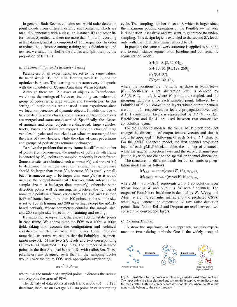
Fig. 5. The illustration of automotive radar settings in radarscenes dataset[1]. The figure is reproduced from [1]. The four radars are mounted at thefront end of the vehicle at 85◦, 25◦, −25◦, and −85◦ with respect to thedriver, respectively. Each radar covers a ±60◦ field of view.

Moreover, a channel projection layer is used in the beginningand the end of the block to mix different components ofeach feature along the channel dimension, which makes thelearned features more flexible. In general, gMLP is superiorthan the MLP-Mixer whose block is mainly composed of aspacial-mixing MLP and a channel-mixing MLP, as gMLPcan be seen as an improved version of the MLP-Mixer bycombining SGU with the latter. By incorporating gMLP intoour proposed network, a beneficial mixture of local and globalfeatures can be retrieved adaptively from all points at a singleframe, allowing for correct semantic guidance while takinginto account differences in sparsity of radar detection pointsfrom one frame to another.

The performance of the network with gMLP as well as withother visual MLPs are compared and analyzed in Section IV.

IV. EXPERIMENTS AND RESULTS

A. Dataset

RadarScenes [1] dataset is selected to validate the proposedmethods. The dataset contains data from four front-mountednear-range automotive radars, one camera, and one odometer.The four radars are 77 GHz near field automotive radar witha detection range of up to 100 meters, mounted at the frontend of the vehicle at 85◦, 25◦, −25◦, and −85◦ with respectto the driver, respectively. Each radar covers a ±60◦ field ofview. The illustration of mounting positions of four radars andthe corresponding field of view (FOV) can be seen in Fig. 5.The data stream is timestamped so that the ego-coordinateof any vehicle can be used as the anchor coordinate system,and information from all four radars are synchronized in oneframe. The average frame rate is 17Hz.

The radar provides data of position, velocity, time, and ID,in both Cartesian and polar coordinates. Among these data,the followings are useful: RCS in dBsm; vr compensatedin meter/second (m/s), which is the radial velocity for thisdetection but compensated for the ego-motion; x cc / y ccin meters, which is the position of the detection horizontal /orthogonal to the car in the car coordinate system (the originis at the center of the rear-axle).

6

In general, RadarScenes contains real-world radar detectionpoint clouds from different driving environments, which aremanually annotated with a class, an instance ID and other in-formation. Specifically, there are more than 4 hours’ recordingin this dataset, and it is composed of 158 sequences. In orderto reduce the difference among training set, validation set andtest set, we randomly shuffle the frames and split them by theproportion of 8 : 1 : 1.

B. Implementation and Parameter Setting

Parameters of all experiments are set to the same values:the batch size is 512, the initial learning rate is 10−3, and theoptimizer is Adam. The learning rate restarts every 20 epochswith the scheduler of Cosine Annealing Warm Restarts.

Although there are 12 classes of objects in RadarScenes,we choose the settings of 5 classes, including car, pedestrian,group of pedestrians, large vehicle and two-wheeler. In thissetting, all static points are not used in our experiment sincewe focus on detection of dynamic objects. In addition, due tolack of data in some classes, some classes of dynamic objectsare merged and some are discarded. Specifically, the classesof animals and other objects are discarded; large vehicles,trucks, buses and trains are merged into the class of largevehicles, bicycles and motorized two-wheelers are merged intothe class of two-wheelers, while the class of cars, pedestriansand groups of pedestrians remains unchanged.

To solve the problem that every frame has different numberof points (for convenience, the number of points in i-th frameis denoted by Ni), points are sampled randomly in each frame.Some statistics are obtained such as max(Ni) and mean(Ni)to determine the sample size. In training, the sample sizeshould be larger than most Nis because Ni is usually small,but it is unnecessary to be larger than max(Ni) as it wouldincrease the computational cost. However, while inferring, thesample size must be larger than max(Ni), otherwise somedetection points will be missing. In practice, the number ofnon-static points in a frame varies from 1 to 173, and less than0.4% of frames have more than 100 points, so the sample sizeis set to 100 in training and 200 in testing, except the gMLP-based network, whose parameters contains the sample size,and 200 sample size is set in both training and testing.

By sampling (or repeating), there exist 100 non-static pointsin each frame. We approximate the FOV to a 100m × 100mfield, taking into account the configuration and technicalspecification of the four near field radars. Based on thesenumerical structures, we require that the PointNet++ segmen-tation network [6] has two SA levels and two correspondingFP levels, as illustrated in Fig. 3(a). The number of sampledpoints in the first SA level is set to 64 with radius 8m. Theseparameters are designed such that all the sampling cycleswould cover the entire FOV with appropriate overlapping:

nπr2 > SFOV,

where n is the number of sampled points; r denotes the radius;and SFOV is the area of FOV.

The density of data points at each frame is 300/64 = 3.125;therefore, there are on average 3.1 data points in each sampling

cycle. The sampling number is set to 8 which is larger sincethe maximum pooling operation of the PointNet++ networkis duplication insensitive and we want to guarantee no under-sampling. This design logic is extended to the second SA level,only with the input data being reduced to 64.

In practice, the same network structure is applied to both theend-to-end instance segmentation baseline and our semanticsegmentation model:

SA(64, 8, [8, 32, 64]),

SA(16, 16, [64, 128, 256]),

FP (64, 32),

FP (32, 32, 16),

where the notations are the same as those in PointNet++[6]. Specifically, a set abstraction level is denoted bySA(K, r, [l1, · · · , ld]), where K points are sampled, and thegrouping radius is r for each sampled point, followed by aPointNet of d 1×1 convolution layers whose output channelsare l1, · · · , ld, respectively; a feature propagation level withd 1×1 convolution layers is represented by FP (l1, · · · , ld).BatchNorm and ReLU are used between two consecutiveconvolution layers.

For the enhanced models, the visual MLP block does notchange the dimension of output feature vectors and thus itcould be appended in following of each SA or FP directly.For the gMLP enhanced model, the first channel projectionlayer of each gMLP block doubles the number of channels,while the spacial projection layer and the second channel pro-jection layer do not change the spacial or channel dimension.

The structures of different heads for our semantic segmen-tation model are as follows:

MSEM = conv(conv(F , 16), nclass),

MSHIFT = conv(conv(F , 16), ndim),

where M = conv(X, l) represents a 1× 1 convolution layerwhose input is X and output is M with l channels. Theoutput of PointNet++ backbone is denoted by F . MSEM andMSHIFT are the semantic matrix and the predicted CSVs,while ndim denotes the dimension of raw radar detectionpoints. BatchNorm, ReLU and Dropout are used between twoconsecutive convolution layers.

C. Existing Methods

To show the superiority of our approach, we also experi-ment on two existing methods. One is the widely accepted

/18

Clustering based Classification

Ø BaselineØ Clustering: DBSCAN / SRV-DBSCAN / EDBSCANØ Classification: Random Forest Classifier using hand-crafted

features

8

Clustering Classification

Original Detection Points Predicted Instance Segmentation Results

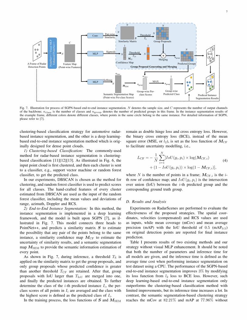
Fig. 6. Illustration for the process of clustering-based classification method.The input points are first clustered and a classifier is applied to predict a classfor each cluster. Different colors denote different classes, where points in thesame circle belong to the same instance.

7

C

N

Conv N

N

nclass

N

Similarity Matrix

Confidence Map

Semantic Segmentation Map(Point-wise Per-class Scores)

N

S

MSEM

MCF

N

N

N

N ×Threshold

TCF

ThresholdTS

Group Proposal Generating and Merging

nclass

ngroup

Group-wise Per-class Scores

ngroup

MAX

Group-wise Predicted Class

ngroup

1

1 1

MLP

MLP

A Frame of Radar Detection Points

Predicted Groups

Prediced Instance Segmentation Results

Pair-wise Similarity

Sigmoid

Softmax

Feature Map(Point-wise Features)Po

intN

et++

/ Vi

sual

MLP

En

hanc

ed P

oint

Net

++

Merging

Group Proposals

Fig. 7. Illustration for process of SGPN-based end-to-end instance segmentation. N denotes the sample size, and C represents the number of output channelsof the backbone; nclass is the number of classes and ngroup denotes the number of predicted groups in this frame. In the instance segmentation results ofthe example frame, different colors denote different classes, where points in the same circle belong to the same instance. For detailed information of SGPN,please refer to [7].

clustering-based classification strategy for automotive radar-based instance segmentation, and the other is a deep learning-based end-to-end instance segmentation method which is orig-inally designed for dense point clouds.

1) Clustering-based Classification: The commonly-usedmethod for radar-based instance segmentation is clustering-based classification [11][12][13]. As illustrated in Fig. 6, theinput point cloud is first clustered, and then each cluster is sentto a classifier, e.g., support vector machine or random forestclassifier, to get the predicted class.

In our experiments, DBSCAN is chosen as the method forclustering, and random forest classifier is used to predict scoresfor all classes. The hand-crafted features of every clusterestimated from DBSCAN are used as the input of the randomforest classifier, including the mean values and deviations ofrange, azimuth, Doppler and RCS.

2) End-to-End Instance Segmentation: In this method, theinstance segmentation is implemented in a deep learningframework, and the model is built upon SGPN [7], as il-lustrated in Fig. 7. This model connects three heads toPointNet++, and predicts a similarity matrix S to estimatethe possibility that any pair of the points belong to the sameinstance, a similarity confidence map MCF to estimate theuncertainty of similarity results, and a semantic segmentationmap MSEM to provide the semantic information estimation ofevery point.

As shown in Fig. 7, during inference, a threshold TS isapplied on the similarity matrix to get the group proposals, andonly group proposals whose predicted confidence is greaterthan another threshold TCF are retained. After that, groupproposals with IoU larger than TIoU are merged into one,and finally the predicted instances are obtained. To furtherdetermine the class of the i-th predicted instance Ii, the per-class scores of all points in Ii are averaged and the class withthe highest score is defined as the predicted class of Ii.

In the training process, the loss functions of S and MSEM

remain as double hinge loss and cross entropy loss. However,the binary cross entropy loss (BCE), instead of the meansquare error (MSE, or l2), is set as the loss function of MCF

to facilitate uncertainty modelling, i.e.,

LCF =− 1

N

N∑i=1

[IoU(gi, pi)× log(MCF,i)

+ (1− IoU(gi, pi))× log(1−MCF,i)],

(4)

where N is the number of points in a frame; MCF,i is the i-th row of confidence map; and IoU(gi, pi) is the intersectionover union (IoU) between the i-th predicted group and thecorresponding ground truth group.

D. Results and Analysis

Experiments on RadarScenes are performed to evaluate theeffectiveness of the proposed strategies. The spatial coor-dinates, velocities (compensated) and RCS values are usedas inputs, while mean coverage (mCov) and mean averageprecision (mAP) with the IoU threshold of 0.5 (mAP0.5)on original detection points are reported for final instanceprediction.

Table I presents results of two existing methods and ourstrategy without visual MLP enhancement. It should be notedthat both the number of parameters and inference time forall models are given, and the inference time is defined as theaverage time cost when performing instance segmentation ontest dataset using a CPU. The performance of the SGPN-basedend-to-end instance segmentation improves 3% by modifyingits loss function from l2 loss to BCE loss. However, suchdeep learning-based end-to-end instance segmentation onlyoutperforms the clustering-based classification method withlimited improvements, but its inference time increases a lot. Incontrast, the semantic segmentation-based clustering strategyreaches the mCov at 82.21% and mAP at 77.96% without

8

TABLE IRESULTS OF DIFFERENT STRATEGIES FOR INSTANCE SEGMENTATION ON TEST DATA

Method Model mCov(%) mAP0.5(%) #Params/Memory Inference TimeClustering-based

ClassificationDBSCAN + Random

Forest Classifier - 79.54 76.09 - / - 17.1ms

End-to-EndInstance Seg. SGPN l2 Loss for MCF 77.32 73.21 75.8K/0.326MB 63.8ms

Our BCE Loss for MCF 79.91 76.15 75.8K/0.326MB 63.8ms

Semantic Seg.based Clustering

PointNet+++ DBSCAN

Without CSV Head 82.21 77.96 75.2K/0.320MB 27.4msWith CSV Head, l2 Loss 82.38 78.17 75.6K/0.324MB 28.7ms

With CSV Head, CS&NIP Loss 82.78 79.38 75.6K/0.324MB 28.7ms

TABLE IIRESULTS OF DIFFERENT ENHANCED MODELS ON TEST DATA

Method Model Enhancement mCov(%) mAP0.5(%) #Params/Memory Inference TimeEnd-to-End

Instance Seg.SGPN (Our BCELoss for MCF)

- 79.91 76.15 75.8K/0.326MB 63.8msgMLP 84.11 81.09 339.9K/1.346MB 336.3ms

Semantic Seg.based Clustering

PointNet++ (withCSV Head, CS&NIP

Loss) + DBSCAN

- 82.78 79.38 75.6K/0.324MB 28.7msgMLP 88.54 85.24 339.7K/1.306MB 32.5msaMLP 89.53 86.97 435.0K/1.714MB 35.4ms

External Attention 85.23 81.41 122.7K/0.507MB 31.2msSelf Attention 85.85 82.32 218.2K/0.876MB 32.0msJOURNAL OF LATEX CLASS FILES, VOL. 1, NO. 1, MAY 2020 7

/1818

The output feature map of PointNet++

B C'

N F

B D+C

N

Predicted Center Shift

Vectors

MLP

MLP

softmax

B N_class

NSemantic Matrix

0

0.2

0.4

0.6

0.8

1

1.2

0 0.2 0.4 0.6 0.8 1

Prec

isio

n

Recall

Fig. 6. The PR curve of the example. The blue line is the original PR curveand the orange line is the adjusted PR curve. The area of the shaded part isAP.

TABLE IIIRESULTS OF CLUSTERING BASED CLASSIFICATION ON TEST DATA

Method mCov(%) mAP0.5(%)DBSCAN + Random Forest Classifier 0.7954 0.7609

SRV-DBSCAN + Random Forest Classifier 0.7948 0.7598

the optimal searching radius. To make fair comparison, thesame random forest classifier trained on training set is usedin these two experiments. The results show our method is alittle worse than the traditional one, so we use the originalDBSCAN as clustering method for the strategy of semanticsegmentation based clustering.

Table IV presents the result of baseline and our two strate-gies, including the original version of them. The performanceof the SGPN improves about ***% by simply modifying itsloss function. However, it still do not outperform the baseline.The semantic segmentation based clustering strategy reachesthe mAP of about 78%, while further improvement can bemade by adding a center shift vectors prediction branch toPointNet++.

The experimental results of the enhanced models are sum-marized in Table V. To show the effectiveness of gMLPbased model, we also use external attention and self attentionfor semantic segmentation network for comparison. Com-pared with the original version, the gMLP based PointNet++performs better by nearly 6%, while the self attention andexternal attention based model only gets an improvementof about 3% and 2%, respectively. Notably, by attaching atiny attention module to the spatial gating unit, the aMLPbased model makes further improvement without increasingtoo much inference time. (Jianan comment: Reasons for thatgMLP outperforms self attention and external attention?). ForSGPN, gMLP also makes it outperforms the baseline byaround 5%. Based on the results, we prove that gMLP couldbe a good replacement of self attention in the field of pointcloud processing.

Some examples of instance segmentation results are vi-sualized in Fig.7 and Fig.8. Jianan comment: It is easy tosee from Fig8 that the performance of instance segmentationcould potentially be improved by incorporating the consistentinformation from consecutive frames, e.g. a car identified at

−0.04 −0.02 0.00 0.02 0.04−0.050.000.05

CAR LARGE_VEHICLE NOISE

−100 −50 0 50 100x/m

−5

0

5

y/m

(a)

−100 −50 0 50 100x/m

−5

0

5

y/m

(b)

−100 −50 0 50 100x/m

−5

0

5

y/m

(e)

−100 −50 0 50 100x/m

−5

0

5

y/m

(f)

−100 −50 0 50 100x/m

−5

0

5

y/m

(c)

−100 −50 0 50 100x/m

−5

0

5

y/m

(d)

Fig. 7. Visualization of typical instance segmentation results by using differentstrategies. Different shapes represent different semantics, and different colorsin the same class (same shape) denotes different instances. (a) Ground Truthfor instance segmentation. (b) Instance segmentation results using the strategyof clustering based classification. (c) Instance segmentation results usingthe strategy of end to end instance segmentation. (d) Instance segmentationresults using the strategy of end to end instance segmentation with gMLP.(e) Instance segmentation results using the strategy of semantic segmentationbased clustering. (f) Instance segmentation results using the strategy of gMLPenhanced semantic segmentation based clustering.

previous frame should not be possible to be recognized as apedestrian in the current frame.

V. CONCLUSION AND FURTHER WORK

Jianan comment: We need to rephrase the words aboutconclusion and further work. The conclusion should focus onseveral aspects: semantic segmentation based clustering strat-egy could provide not only the best performance in mmCovand mmAP, but also much faster than end to end instancesegmentation strategy. The inference time does not increasethat much compared to baseline clustering + classificationstrategy, however the performance shows significant better.The gMLP enhanced semantic segmentation based clusteringcan provide greatly improvement in mmCov and mmAP, butthe inference time only increases slightly compared to the onewithout gMLP, thus makes our proposed approach feasible forthe real-time radar based ADAS/AD product. In this paper,we propose two strategies for radar point cloud instancesegmentation. One is end to end instance segmentation usingSGPN, and the other is semantic segmentation based clusteringby PointNet++ and DBSCAN. After we carefully decide the

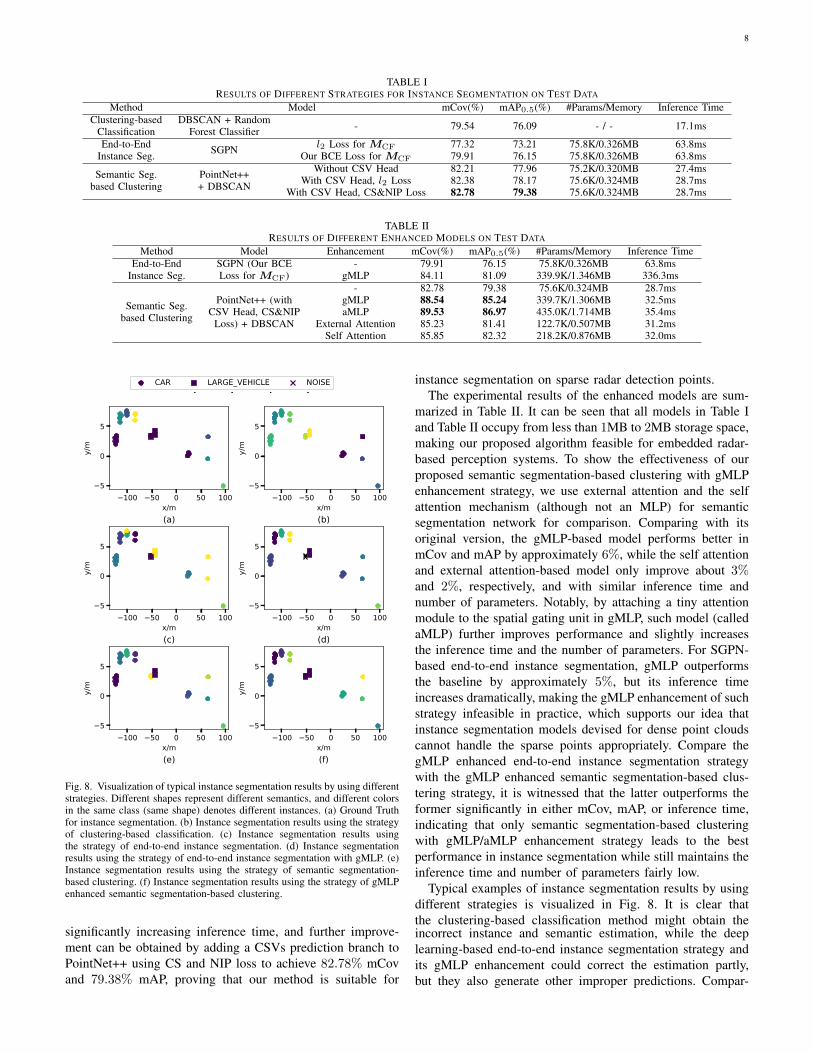
Fig. 8. Visualization of typical instance segmentation results by using differentstrategies. Different shapes represent different semantics, and different colorsin the same class (same shape) denotes different instances. (a) Ground Truthfor instance segmentation. (b) Instance segmentation results using the strategyof clustering-based classification. (c) Instance segmentation results usingthe strategy of end-to-end instance segmentation. (d) Instance segmentationresults using the strategy of end-to-end instance segmentation with gMLP. (e)Instance segmentation results using the strategy of semantic segmentation-based clustering. (f) Instance segmentation results using the strategy of gMLPenhanced semantic segmentation-based clustering.

significantly increasing inference time, and further improve-ment can be obtained by adding a CSVs prediction branch toPointNet++ using CS and NIP loss to achieve 82.78% mCovand 79.38% mAP, proving that our method is suitable for

instance segmentation on sparse radar detection points.The experimental results of the enhanced models are sum-

marized in Table II. It can be seen that all models in Table Iand Table II occupy from less than 1MB to 2MB storage space,making our proposed algorithm feasible for embedded radar-based perception systems. To show the effectiveness of ourproposed semantic segmentation-based clustering with gMLPenhancement strategy, we use external attention and the selfattention mechanism (although not an MLP) for semanticsegmentation network for comparison. Comparing with itsoriginal version, the gMLP-based model performs better inmCov and mAP by approximately 6%, while the self attentionand external attention-based model only improve about 3%and 2%, respectively, and with similar inference time andnumber of parameters. Notably, by attaching a tiny attentionmodule to the spatial gating unit in gMLP, such model (calledaMLP) further improves performance and slightly increasesthe inference time and the number of parameters. For SGPN-based end-to-end instance segmentation, gMLP outperformsthe baseline by approximately 5%, but its inference timeincreases dramatically, making the gMLP enhancement of suchstrategy infeasible in practice, which supports our idea thatinstance segmentation models devised for dense point cloudscannot handle the sparse points appropriately. Compare thegMLP enhanced end-to-end instance segmentation strategywith the gMLP enhanced semantic segmentation-based clus-tering strategy, it is witnessed that the latter outperforms theformer significantly in either mCov, mAP, or inference time,indicating that only semantic segmentation-based clusteringwith gMLP/aMLP enhancement strategy leads to the bestperformance in instance segmentation while still maintains theinference time and number of parameters fairly low.

Typical examples of instance segmentation results by usingdifferent strategies is visualized in Fig. 8. It is clear thatthe clustering-based classification method might obtain theincorrect instance and semantic estimation, while the deeplearning-based end-to-end instance segmentation strategy andits gMLP enhancement could correct the estimation partly,but they also generate other improper predictions. Compar-

9JOURNAL OF LATEX CLASS FILES, VOL. 1, NO. 1, MAY 2020 8

−0.04 −0.02 0.00 0.02 0.04−0.050.000.05

CAR PEDESTRIAN PEDESTRIAN_GROUP LARGE_VEHICLE

0 100x/m

0

5

10y/m

0 100x/m

0

5

10

y/m

0 100x/m

0

5

10

y/m

0 100x/m

0

5

10y/m

0 100x/m

0

5

10

y/m

0 100x/m

0

5

10

y/m

0 100x/m

0

5

10

y/m

0 100x/m

0

5

10

y/m

0 100x/m

−5

0

5

10

y/m

0 100x/m

−5

0

5

10

y/m

Fig. 8. Visualization of typical instance segmentation results in several consecutive frames. Strategy of gMLP enhanced semantic segmentation based clusteringis used to generate these figures. The first row is the ground truth for instance segmentation, and the second row is the predicted instance segmentation results.

segmentation strategy. The inference time does not increasethat much compared to baseline clustering + classificationstrategy, however the performance shows significant better.The gMLP enhanced semantic segmentation based clusteringcan provide greatly improvement in mmCov and mmAP, butthe inference time only increases slightly compared to the onewithout gMLP, thus makes our proposed approach feasible forthe real-time radar-based ADAS/AD product.

In this paper, we propose two strategies for radar point cloudinstance segmentation. One is end-to-end instance segmenta-tion using SGPN, and the other is semantic segmentation basedclustering by PointNet++ and DBSCAN. The latter strategynot only provide better mCov and mAP than the former one,but also much faster while inferring. The inference time ofthe latter method does not increase much compared to thebaseline, whereas the performance shows significantly better.

After we carefully decide the model parameters and com-pare the effect of different loss functions, an enhancementwith gMLP is introduced. The gMLP enhanced semanticsegmentation based clustering can provide great improvementin mCov and mAP, but the inference time only increasesslightly compared to the one without gMLP, thus makesour proposed approach feasible for the real-time radar-basedADAS/AD product.

However, we only use single frame for training the modeland predicting the instance information even if the datasetprovides sequences of radar point clouds, i.e. point cloudvideos. Taking point clouds of several consecutive frames intoaccount at the same time might enable the model to extractmore features and facilitate learning, which is worth studyingin the future. Another work that is necessary is to reduce themodel size and number of FLOPs while inferring, becauseradar perception programs are usually stored in an embeddedsystem and no GPU is available, so the characteristic of light-weight is essential to our models.

ACKNOWLEDGMENT

The authors would like to thank...

REFERENCES

[1] C. Qi, H. Su, K. Mo, and L. Guibas, “Pointnet: Deep learning on pointsets for 3d classification and segmentation,” 2017 IEEE Conference onComputer Vision and Pattern Recognition (CVPR), pp. 77–85, 2017.

[2] C. Qi, L. Yi, H. Su, and L. Guibas, “Pointnet++: Deep hierarchicalfeature learning on point sets in a metric space,” in NIPS, 2017.

[3] R. Zhang and S. Cao, “Robust and adaptive radar elliptical density-basedspatial clustering and labeling for mmwave radar point cloud data,” 201953rd Asilomar Conference on Signals, Systems, and Computers, pp. 919–924, 2019.

[4] T. Wagner, R. Feger, and A. Stelzer, “Modification of dbscan and ap-plication to range/doppler/doa measurements for pedestrian recognitionwith an automotive radar system,” 2015 European Radar Conference(EuRAD), pp. 269–272, 2015.

[5] D. Birant and A. Kut, “St-dbscan: An algorithm for clustering spatial-temporal data,” Data Knowl. Eng., vol. 60, pp. 208–221, 2007.

[6] W. Wang, R. Yu, Q. Huang, and U. Neumann, “Sgpn: Similarity groupproposal network for 3d point cloud instance segmentation,” 2018IEEE/CVF Conference on Computer Vision and Pattern Recognition,pp. 2569–2578, 2018.

[7] S. Chen, J. Fang, Q. Zhang, W. Liu, and X. Wang, “Hierarchicalaggregation for 3d instance segmentation,” ArXiv, vol. abs/2108.02350,2021.

[8] I. Tolstikhin, N. Houlsby, A. Kolesnikov, L. Beyer, X. Zhai, T. Un-terthiner, J. Yung, D. Keysers, J. Uszkoreit, M. Lucic, and A. Doso-vitskiy, “Mlp-mixer: An all-mlp architecture for vision,” ArXiv, vol.abs/2105.01601, 2021.

[9] S. Chen, E. Xie, C. Ge, D. Liang, and P. Luo, “Cyclemlp: A mlp-likearchitecture for dense prediction,” ArXiv, vol. abs/2107.10224, 2021.

[10] H. Liu, Z. Dai, D. R. So, and Q. V. Le, “Pay attention to mlps,” ArXiv,vol. abs/2105.08050, 2021.

[11] M.-H. Guo, Z.-N. Liu, T.-J. Mu, and S. Hu, “Beyond self-attention:External attention using two linear layers for visual tasks,” ArXiv, vol.abs/2105.02358, 2021.

[12] A. Danzer, T. Griebel, M. Bach, and K. Dietmayer, “2d car detection inradar data with pointnets,” 2019 IEEE Intelligent Transportation SystemsConference (ITSC), pp. 61–66, 2019.

[13] J. F. Tilly, S. Haag, O. Schumann, F. Weishaupt, B. Duraisamy, J. Dick-mann, and M. Fritzsche, “Detection and tracking on automotive radardata with deep learning,” 2020 IEEE 23rd International Conference onInformation Fusion (FUSION), pp. 1–7, 2020.

[14] J. Bai, L. Zheng, S. Li, B. Tan, S. Chen, and L. Huang, “Radartransformer: An object classification network based on 4d mmw imagingradar,” Sensors (Basel, Switzerland), vol. 21, 2021.

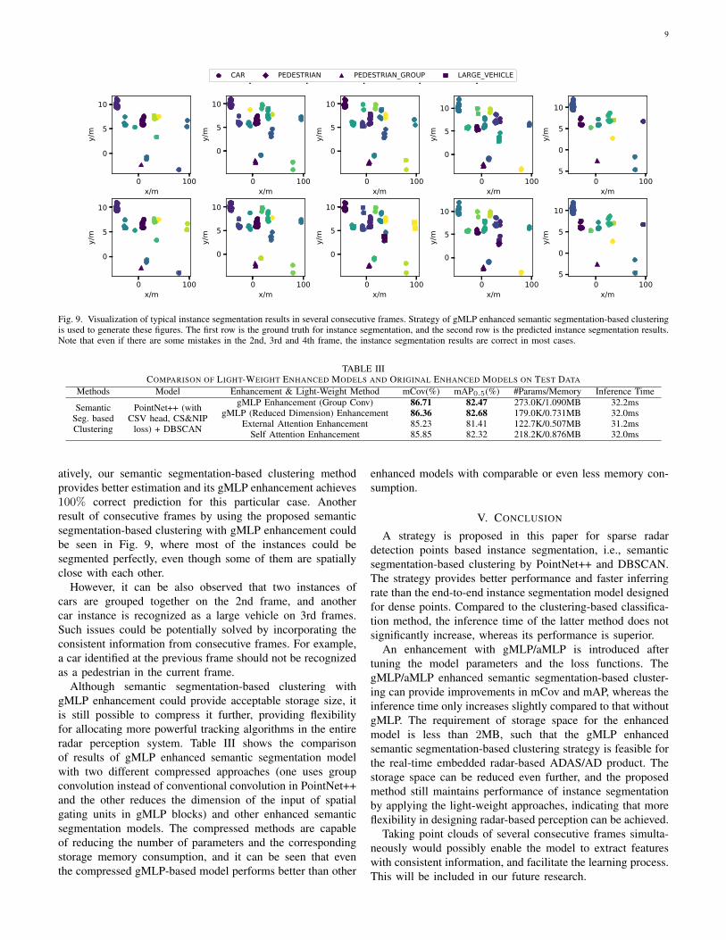
Fig. 9. Visualization of typical instance segmentation results in several consecutive frames. Strategy of gMLP enhanced semantic segmentation-based clusteringis used to generate these figures. The first row is the ground truth for instance segmentation, and the second row is the predicted instance segmentation results.Note that even if there are some mistakes in the 2nd, 3rd and 4th frame, the instance segmentation results are correct in most cases.

TABLE IIICOMPARISON OF LIGHT-WEIGHT ENHANCED MODELS AND ORIGINAL ENHANCED MODELS ON TEST DATA

Methods Model Enhancement & Light-Weight Method mCov(%) mAP0.5(%) #Params/Memory Inference Time

SemanticSeg. basedClustering

PointNet++ (withCSV head, CS&NIP

loss) + DBSCAN

gMLP Enhancement (Group Conv) 86.71 82.47 273.0K/1.090MB 32.2msgMLP (Reduced Dimension) Enhancement 86.36 82.68 179.0K/0.731MB 32.0ms

External Attention Enhancement 85.23 81.41 122.7K/0.507MB 31.2msSelf Attention Enhancement 85.85 82.32 218.2K/0.876MB 32.0ms

atively, our semantic segmentation-based clustering methodprovides better estimation and its gMLP enhancement achieves100% correct prediction for this particular case. Anotherresult of consecutive frames by using the proposed semanticsegmentation-based clustering with gMLP enhancement couldbe seen in Fig. 9, where most of the instances could besegmented perfectly, even though some of them are spatiallyclose with each other.

However, it can be also observed that two instances ofcars are grouped together on the 2nd frame, and anothercar instance is recognized as a large vehicle on 3rd frames.Such issues could be potentially solved by incorporating theconsistent information from consecutive frames. For example,a car identified at the previous frame should not be recognizedas a pedestrian in the current frame.

Although semantic segmentation-based clustering withgMLP enhancement could provide acceptable storage size, itis still possible to compress it further, providing flexibilityfor allocating more powerful tracking algorithms in the entireradar perception system. Table III shows the comparisonof results of gMLP enhanced semantic segmentation modelwith two different compressed approaches (one uses groupconvolution instead of conventional convolution in PointNet++and the other reduces the dimension of the input of spatialgating units in gMLP blocks) and other enhanced semanticsegmentation models. The compressed methods are capableof reducing the number of parameters and the correspondingstorage memory consumption, and it can be seen that eventhe compressed gMLP-based model performs better than other

enhanced models with comparable or even less memory con-sumption.

V. CONCLUSION

A strategy is proposed in this paper for sparse radardetection points based instance segmentation, i.e., semanticsegmentation-based clustering by PointNet++ and DBSCAN.The strategy provides better performance and faster inferringrate than the end-to-end instance segmentation model designedfor dense points. Compared to the clustering-based classifica-tion method, the inference time of the latter method does notsignificantly increase, whereas its performance is superior.

An enhancement with gMLP/aMLP is introduced aftertuning the model parameters and the loss functions. ThegMLP/aMLP enhanced semantic segmentation-based cluster-ing can provide improvements in mCov and mAP, whereas theinference time only increases slightly compared to that withoutgMLP. The requirement of storage space for the enhancedmodel is less than 2MB, such that the gMLP enhancedsemantic segmentation-based clustering strategy is feasible forthe real-time embedded radar-based ADAS/AD product. Thestorage space can be reduced even further, and the proposedmethod still maintains performance of instance segmentationby applying the light-weight approaches, indicating that moreflexibility in designing radar-based perception can be achieved.

Taking point clouds of several consecutive frames simulta-neously would possibly enable the model to extract featureswith consistent information, and facilitate the learning process.This will be included in our future research.

10

REFERENCES

[1] O. Schumann, M. Hahn, N. Scheiner, F. Weishaupt, J. F.Tilly, J. Dickmann, and C. Wohler, “Radarscenes: A real-worldradar point cloud data set for automotive applications,” 2021IEEE 24th International Conference on Information Fusion(FUSION), pp. 1–8, 2021.

[2] Y. Liu, Q. Hu, Y. Zou, and W. Wang, “Labelled non-zeroparticle flow for smc-phd filtering,” in ICASSP 2019-2019IEEE International Conference on Acoustics, Speech and SignalProcessing (ICASSP). IEEE, 2019, pp. 5197–5201.

[3] C. Waldschmidt, J. Hasch, and W. Menzel, “Automotive radar— from first efforts to future systems,” IEEE Journal ofMicrowaves, vol. 1, pp. 135–148, 2021.

[4] S. Chen, B. Liu, C. Feng, C. Vallespi-Gonzalez, and C. K.Wellington, “3d point cloud processing and learning for au-tonomous driving,” IEEE Signal Processing Magazine, SpecialIssue on Autonomous Driving, pp. 68–86, 2021.

[5] C. Qi, H. Su, K. Mo, and L. Guibas, “Pointnet: Deep learningon point sets for 3d classification and segmentation,” 2017IEEE Conference on Computer Vision and Pattern Recognition(CVPR), pp. 77–85, 2017.

[6] C. Qi, L. Yi, H. Su, and L. Guibas, “Pointnet++: Deep hierar-chical feature learning on point sets in a metric space,” in NIPS,2017.

[7] W. Wang, R. Yu, Q. Huang, and U. Neumann, “Sgpn: Similaritygroup proposal network for 3d point cloud instance segmen-tation,” 2018 IEEE/CVF Conference on Computer Vision andPattern Recognition, pp. 2569–2578, 2018.

[8] S. Chen, J. Fang, Q. Zhang, W. Liu, and X. Wang, “Hierarchicalaggregation for 3d instance segmentation,” 2021 IEEE/CVF In-ternational Conference on Computer Vision (ICCV), pp. 15 447–15 456, 2021.

[9] A. Danzer, T. Griebel, M. Bach, and K. Dietmayer, “2d cardetection in radar data with pointnets,” 2019 IEEE IntelligentTransportation Systems Conference (ITSC), pp. 61–66, 2019.

[10] M. Ester, H.-P. Kriegel, J. Sander, and X. Xu, “A density-basedalgorithm for discovering clusters in large spatial databases withnoise,” in KDD, 1996.

[11] Y. Liu, A. Hilton, J. Chambers, Y. Zhao, and W. Wang, “Non-zero diffusion particle flow smc-phd filter for audio-visualmulti-speaker tracking,” in 2018 IEEE International Conferenceon Acoustics, Speech and Signal Processing (ICASSP). IEEE,2018, pp. 4304–4308.

[12] N. Scheiner, O. Schumann, F. Kraus, N. Appenrodt, J. Dick-mann, and B. Sick, “Off-the-shelf sensor vs. experimentalradar - how much resolution is necessary in automotive radarclassification?” 2020 IEEE 23rd International Conference onInformation Fusion (FUSION), pp. 1–8, 2020.

[13] X. Gao, G. Xing, S. Roy, and H. Liu, “Experiments withmmwave automotive radar test-bed,” 2019 53rd Asilomar Con-ference on Signals, Systems, and Computers, pp. 1–6, 2019.

[14] M.-H. Guo, Z.-N. Liu, T.-J. Mu, and S. Hu, “Beyond self-attention: External attention using two linear layers for visualtasks,” ArXiv, vol. abs/2105.02358, 2021.

[15] I. Tolstikhin, N. Houlsby, A. Kolesnikov, L. Beyer, X. Zhai,T. Unterthiner, J. Yung, D. Keysers, J. Uszkoreit, M. Lucic,and A. Dosovitskiy, “Mlp-mixer: An all-mlp architecture forvision,” ArXiv, vol. abs/2105.01601, 2021.

[16] H. Liu, Z. Dai, D. R. So, and Q. V. Le, “Pay attention to mlps,”ArXiv, vol. abs/2105.08050, 2021.

[17] A. Dosovitskiy, L. Beyer, A. Kolesnikov, D. Weissenborn,X. Zhai, T. Unterthiner, M. Dehghani, M. Minderer, G. Heigold,S. Gelly, J. Uszkoreit, and N. Houlsby, “An image is worth16x16 words: Transformers for image recognition at scale,”ArXiv, vol. abs/2010.11929, 2021.

[18] X. Dong, J. Bao, D. Chen, W. Zhang, N. Yu, L. Yuan,D. Chen, and B. Guo, “Cswin transformer: A general visiontransformer backbone with cross-shaped windows,” ArXiv, vol.abs/2107.00652, 2021.

[19] Z. Liu, Y. Lin, Y. Cao, H. Hu, Y. Wei, Z. Zhang, S. Lin, andB. Guo, “Swin transformer: Hierarchical vision transformer us-ing shifted windows,” 2021 IEEE/CVF International Conferenceon Computer Vision (ICCV), pp. 9992–10 002, 2021.

[20] A. Vaswani, N. M. Shazeer, N. Parmar, J. Uszkoreit, L. Jones,A. N. Gomez, L. Kaiser, and I. Polosukhin, “Attention is allyou need,” ArXiv, vol. abs/1706.03762, 2017.

[21] S. Chen, E. Xie, C. Ge, D. Liang, and P. Luo, “Cyclemlp:A mlp-like architecture for dense prediction,” ArXiv, vol.abs/2107.10224, 2021.

[22] N. Scheiner, N. Appenrodt, J. Dickmann, and B. Sick, “A multi-stage clustering framework for automotive radar data,” 2019IEEE Intelligent Transportation Systems Conference (ITSC), pp.2060–2067, 2019.

[23] O. Schumann, M. Hahn, J. Dickmann, and C. Wohler, “Seman-tic segmentation on radar point clouds,” 2018 21st InternationalConference on Information Fusion (FUSION), pp. 2179–2186,2018.

[24] J. F. Tilly, S. Haag, O. Schumann, F. Weishaupt, B. Duraisamy,J. Dickmann, and M. Fritzsche, “Detection and tracking onautomotive radar data with deep learning,” 2020 IEEE 23rdInternational Conference on Information Fusion (FUSION), pp.1–7, 2020.

[25] S. Haag, B. Duraisamy, F. Govaers, W. Koch, M. Fritzsche,and J. Dickmann, “Extended object tracking assisted adaptiveclustering for radar in autonomous driving applications,” 2019Sensor Data Fusion: Trends, Solutions, Applications (SDF), pp.1–7, 2019.

[26] R. Prophet, A. Deligiannis, J.-C. Fuentes-Michel, I. Weber, andM. Vossiek, “Semantic segmentation on 3d occupancy grids forautomotive radar,” IEEE Access, vol. 8, pp. 197 917–197 930,2020.

[27] Y. Liu, V. Kılıc, J. Guan, and W. Wang, “Audio–visual par-ticle flow smc-phd filtering for multi-speaker tracking,” IEEETransactions on Multimedia, vol. 22, no. 4, pp. 934–948, 2019.

[28] C. Wohler, O. Schumann, M. Hahn, and J. Dickmann, “Com-parison of random forest and long short-term memory networkperformances in classification tasks using radar,” 2017 SensorData Fusion: Trends, Solutions, Applications (SDF), pp. 1–6,2017.