INFLOW PERFORMANCE RELATIONSHIPS (IPR) FOR SOLUTION GAS DRIVE RESERVOIRS — A SEMI-ANALYTICAL APPROACH A Thesis by MARÍA ALEJANDRA NASS Submitted to the Office of Graduate Studies of Texas A&M University in partial fulfillment of the requirements for the degree of MASTER OF SCIENCE May 2010 Major Subject: Petroleum Engineering

Welcome message from author
This document is posted to help you gain knowledge. Please leave a comment to let me know what you think about it! Share it to your friends and learn new things together.
Transcript

INFLOW PERFORMANCE RELATIONSHIPS (IPR) FOR SOLUTION GAS
DRIVE RESERVOIRS — A SEMI-ANALYTICAL APPROACH
A Thesis
by
MARÍA ALEJANDRA NASS
Submitted to the Office of Graduate Studies of Texas A&M University
in partial fulfillment of the requirements for the degree of
MASTER OF SCIENCE
May 2010
Major Subject: Petroleum Engineering
Inflow Performance Relationships (IPR) For Solution Gas Drive Reservoirs —
a Semi-Analytical Approach
Copyright 2010 María Alejandra Nass
INFLOW PERFORMANCE RELATIONSHIPS (IPR) FOR SOLUTION GAS
DRIVE RESERVOIRS — A SEMI-ANALYTICAL APPROACH
A Thesis
by
MARÍA ALEJANDRA NASS
Submitted to the Office of Graduate Studies of Texas A&M University
in partial fulfillment of the requirements for the degree of
MASTER OF SCIENCE Approved by: Co-Chairs of Committee, Thomas A. Blasingame Maria A. Barrufet Committee Member, Robert Weiss Head of Department, Stephen A. Holditch
May 2010
Major Subject: Petroleum Engineering
iii
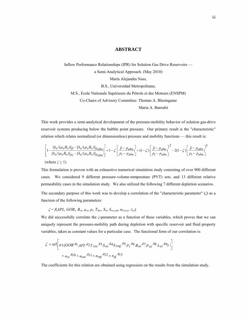
ABSTRACT
Inflow Performance Relationships (IPR) for Solution Gas Drive Reservoirs —
a Semi-Analytical Approach. (May 2010)
María Alejandra Nass,
B.S., Universidad Metropolitana;
M.S., Ecole Nationale Supérieure du Pétrole et des Moteurs (ENSPM)
Co-Chairs of Advisory Committee: Thomas A. Blasingame
Maria A. Barrufet
This work provides a semi-analytical development of the pressure-mobility behavior of solution gas-drive
reservoir systems producing below the bubble point pressure. Our primary result is the "characteristic"
relation which relates normalized (or dimensionless) pressure and mobility functions — this result is:
32
)1(2 )1( 1 )](/[)](/[
)](/[)](/[ 1
abni
abn
abni
abn
abni
abn
abnpoooipooo
abnpooopooo
pp
pp
pp
pp
pp
pp
BkBk
BkBk
(where ζ < 1)
This formulation is proven with an exhaustive numerical simulation study consisting of over 900 different
cases. We considered 9 different pressure-volume-temperature (PVT) sets, and 13 different relative
permeability cases in the simulation study. We also utilized the following 7 different depletion scenarios.
The secondary purpose of this work was to develop a correlation of the "characteristic parameter" (ζ) as a
function of the following parameters:
= f(APIi, GORi, Boi, oi, pi, TRes, Soi, kro,end, nCorey, oi)
We did successfully correlate the ζ-parameter as a function of these variables, which proves that we can
uniquely represent the pressure-mobility path during depletion with specific reservoir and fluid property
variables, taken as constant values for a particular case. The functional form of our correlation is:
ngnnn
BpkSTAPIGOR
Aog
Aow
Aw
A
oiA
oiA
oiA
iA
rogA
oiA
resAAA
13121110
987654321 )(1erf
The coefficients for this relation are obtained using regression on the results from the simulation study.


v
ACKNOWLEDGMENTS
I would like to express my appreciation and gratitude to:
Dr. Tom Blasingame, for his commitment, his patience and, for sharing his time and knowledge
during the time it took to complete this thesis. I thank him for providing such an interesting (and
challenging) subject.
Dr. Maria A. Barrufet, for serving as co-chair of my advisory committee.
Dr. Robert Weiss, for serving as member of my advisory committee.
Dilhan Ilk, for being available for every question I had, and for providing me with the complete
background to initiate this work.
Jose Carballo, for providing me with unlimited encouragement, as well as for many ideas and
support.

vi
TABLE OF CONTENTS
Page
ABSTRACT ...........................................................................................................................................iii
DEDICATION ........................................................................................................................................... iv
ACKNOWLEDGMENTS...............................................................................................................................v
TABLE OF CONTENTS...............................................................................................................................vi
LIST OF FIGURES .....................................................................................................................................viii
LIST OF TABLES..........................................................................................................................................x
CHAPTER I INTRODUCTION..............................................................................................................1
1.1. Research Problem ......................................................................................................................1 1.2. Review of Previous Work..........................................................................................................2 1.3. Present Status of the Problem ....................................................................................................7 1.4. Research Objectives...................................................................................................................9 1.5. Thesis Outline ..........................................................................................................................10
CHAPTER II MODEL-BASED PERFORMANCE OF SOLUTION-GAS-DRIVE RESERVOIRS...11
2.1. Modeling Approach .................................................................................................................11 2.2. Input Data Selection.................................................................................................................13 2.3. Fluid Selection and PVT Properties.........................................................................................15 2.4. Relative Permeability Curves ..................................................................................................25
CHAPTER III CORRELATION OF THE CHARACTERISTIC BEHAVIOR OF SOLUTION-GAS-
DRIVE RESERVOIRS ....................................................................................................31
3.1. Correlation of the -parameter.................................................................................................31 3.2. Validation of the -parameter Correlation ...............................................................................32 3.3. Effect of Input Variables on the -parameter Correlation .......................................................39
CHAPTER IV CONCLUSIONS AND RECOMMENDATIONS...........................................................44
4.1. Conclusions..............................................................................................................................44 4.2. Recommendations for Future Research ...................................................................................44
NOMENCLATURE......................................................................................................................................45

vii
Page REFERENCES ..........................................................................................................................................47
APPENDIX A ..........................................................................................................................................48
APPENDIX B ..........................................................................................................................................49
APPENDIX C ..........................................................................................................................................82
APPENDIX D ..........................................................................................................................................87
APPENDIX E ..........................................................................................................................................92
APPENDIX F ..........................................................................................................................................97
APPENDIX G ........................................................................................................................................102
APPENDIX H ........................................................................................................................................107
APPENDIX I ........................................................................................................................................112
APPENDIX J ........................................................................................................................................117
APPENDIX K ........................................................................................................................................122
APPENDIX L ........................................................................................................................................127
APPENDIX M ........................................................................................................................................132
APPENDIX N ........................................................................................................................................137
APPENDIX O ........................................................................................................................................142
APPENDIX P ........................................................................................................................................147
VITA ........................................................................................................................................151

iv
DEDICATION
I dedicate this thesis to my husband Jose.

ix
FIGURE Page
2.11 Relative permeability curves for kr2, kr7 and kr10 sets (kr2 = base case) ................................... 28
2.12 Relative permeability curves for kr3, kr8 and kr11 sets (kr3 = base case) ................................... 28
2.13 Relative permeability curves for kr1 and kr4 sets (kr1 = base case) ............................................ 29
2.14 Relative permeability curves for kr3 and kr5 sets (kr3 = base case) ............................................ 29
2.15 Relative permeability curves for kr12 set.................................................................................... 30
2.16 Relative permeability curves for kr13 set.................................................................................... 30
3.1 Computed -parameter versus measured -parameter (all data)................................................. 32
3.2 Normalized oil-phase mobility function plotted versus the normalized average reservoir pressure function (Case 1). .......................................................................................... 34
3.3 Derivative of the normalized oil-phase mobility function (taken with respect to the normalized average reservoir pressure function) plotted versus the normalized average reservoir pressure function (Case 1).............................................................................. 35
3.4 Second derivative of the normalized oil-phase mobility function (taken with respect to the normalized average reservoir pressure function) plotted versus the normalized average reservoir pressure function (Case 1).............................................................................. 36
3.5 Integral of the normalized oil-phase mobility function (taken with respect to the normalized average reservoir pressure function) plotted versus the normalized average reservoir pressure function (Case 1).............................................................................. 37
3.6 Integral difference of the normalized oil-phase mobility function (taken with respect to the normalized average reservoir pressure function) plotted versus the normalized average reservoir pressure function (Case 1).............................................................................. 38
3.7 Effect of GOR and API on the computed -parameter. .............................................................. 39
3.8 Effect of reservoir temperature (TRes) on the computed -parameter.......................................... 40
3.9 Effect of initial oil mobility (oi) on the computed -parameter................................................. 41
3.10 Effect of the Corey exponents for the water and gas relative permeabilities (nw and ng) on the computed -parameter. ............................................................................................... 42
3.11 Effect of the Corey exponents for the oil relative permeabilities (nog and now) on the computed -parameter........................................................................................................... 43
x
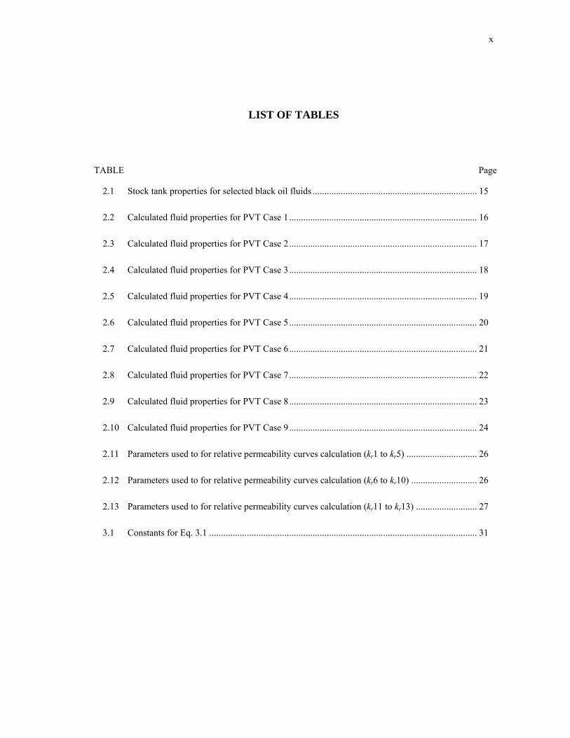
LIST OF TABLES
TABLE Page
2.1 Stock tank properties for selected black oil fluids ...................................................................... 15
2.2 Calculated fluid properties for PVT Case 1................................................................................ 16
2.3 Calculated fluid properties for PVT Case 2................................................................................ 17
2.4 Calculated fluid properties for PVT Case 3................................................................................ 18
2.5 Calculated fluid properties for PVT Case 4................................................................................ 19
2.6 Calculated fluid properties for PVT Case 5................................................................................ 20
2.7 Calculated fluid properties for PVT Case 6................................................................................ 21
2.8 Calculated fluid properties for PVT Case 7................................................................................ 22
2.9 Calculated fluid properties for PVT Case 8................................................................................ 23
2.10 Calculated fluid properties for PVT Case 9................................................................................ 24
2.11 Parameters used to for relative permeability curves calculation (kr1 to kr5) .............................. 26
2.12 Parameters used to for relative permeability curves calculation (kr6 to kr10) ............................ 26
2.13 Parameters used to for relative permeability curves calculation (kr11 to kr13) .......................... 27
3.1 Constants for Eq. 3.1 .................................................................................................................. 31

1
CHAPTER I
INTRODUCTION
1.1. Research Problem
The concept of an Inflow Performance Relationship (IPR) has long been used to predict or estimate the
relationship between pressure drop in the reservoir (drawdown) and well flowrates (production). Such
relationships are used to monitor and optimize the producing life of a reservoir; and also for design
calculations such as estimating tubing sizes, positions of gas lift mandrels, downhole pumps, etc.
Engineers often make use of the IPR to understand the deliverability (or maximum productivity) of a
reservoir, as well as to identify and resolve problems which may arise from the exploitation of a field.
The IPR concept provides an engineer with the means to determine the performance of a given well by
relating inflow (flowrate) to the pressure condition in the well and reservoir at a given time. The most
common application of the IPR concept is to consider the effects of different operational conditions on the
pressure and flowrate profiles for a given well at conditions other than the initial condition.
The development of the IPR approach was initially empirical (Rawlins and Schellhardt 1935), but the IPR
can be defined using the simple "pseudosteady-state" flow relation which provides a direct relationship
between wellbore pressure and flowrate in the reservoir. The underlying relationship between wellbore
pressure and flowrate depends on the conditions — e.g., for a "black oil" produced at pressures above the
bubble-point, the pseudosteady-state flow relation provides a linear relationship between pressure and the
oil flowrate. For the case of a dry gas produced at pressures below approximately 2000-3000 psia, there
exists a linear relationship between gas flowrate and the pressure-squared (i.e., p2). The IPR concept is
designed to relate three variables — flowrate, flowing bottomhole pressure, and the average reservoir
pressure — where each of these variables is evaluated at the same condition (i.e., time).
In this work we focus specifically on the development of IPR equations for solution-gas-drive reservoir
systems (i.e., cases where p < pb); and we assume that the IPR for this case can be represented using some
type of higher degree polynomial form. Such studies have been proposed by others (Vogel 1968,
Richardson and Shaw 1982) — but in our work we focus on the correlation of the oil mobility function,
_________________________
This thesis follows the style and format of the SPE Journal.

2
as we can demonstrate that this is the key performance variable for solution-gas-drive reservoirs.
In this work we use a black oil reservoir simulator (CMG 2008) to generate an exhaustive number of
synthetic performance cases. Using these synthetic results, we have created a correlation for the
dimensionless oil mobility (D,IPR) as a function of a dimensionless pressure (pD,IPR) and a unique
characteristic parameter (). We note that both D,IPR and pD,IPR are both defined using average reservoir
pressure, abandonment pressure, and the flowing bottomhole pressure. The characteristic parameter () is
then correlated with the following fluid and rock-fluid properties:
● (PVT) APIi = Initial Oil Gravity [Deg API] ● (PVT) GORi = Initial Gas-to-Oil Ratio [scf/STB] ● (PVT) Boi = Initial Oil Formation Volume Factor [RB/STB] ● (PVT) oi = Initial Oil Viscosity [cp] ● (Reservoir) pi = Initial Reservoir Pressure [psia] ● (Reservoir) TRes = Reservoir Temperature [Deg F] ● (Reservoir) Soi = Initial (Average) Oil Saturation [fraction] ● (Reservoir) kro,end = Endpoint Oil Relative Permeability [fraction] ● (Reservoir) nCorey = Corey Relative Permeability Exponents [dimensionless] ● (Reservoir) oi = Oil Mobility at Initial Reservoir Pressure [md/cp]
Chapter I of this thesis presents a review of the previous work and theory surrounding IPR formulations.
Chapter II presents the methodology used to develop the all the output from reservoir simulation that was
required to develop the -parameter correlation. We present in this chapter all the data that was used as
well as the polynomial curves that were obtained to describe the oil mobility function.
Chapter III presents the development and validation of the -parameter correlation based on the results
from Chapter II. The detailed methodology and procedure used to analyze the oil mobility calculations
and results is also presented.
Chapter IV presents the summary, conclusions and recommendation for future work.
1.2. Review of Previous Work
1.2.1 IPR for Single-Phase Flow
The development of IPR for single-phase flow is reviewed as it provides the basis of the development of
an IPR for two-phase flow (in this case, the solution gas-drive system). Beginning with the
"pseudosteady-state" flow equation for a single-phase black oil system (Economides, et al. 1994), we
have:
ow
e
o
oowf qs
r
r
hk
Bpp
4
3ln 2.141
(field units) ......................................................................(1.1)

3
Consolidating terms in Eq. 1, we have:
opsswf qbpp ....................................................................................................................................(1.2)
A more common form of Eq. 2 is written in terms of the "productivity index," Jo, is given as:
oo
wf qJ
pp 1
......................................................................................................................................(1.3)
Where Jo is defined in terms of reservoir and production variables (for this case) as:
sr
r
hk
BbJ
w
e
o
oopsso
4
3ln 2.141
11
.............................................................................................(1.4)
And the definition of Jo in terms of the flowrate, the flowing bottomhole pressure at the well, and the average reservoir pressure is given by:
)( wf
oo pp
qJ
.......................................................................................................................................(1.5)
Solving Eq. 5 for the case where pwf=0; we define the maximum oil flowrate (qo,max) as:
pJq oo max, ...........................................................................................................................................(1.6)
Solving Eq. 3 (or Eq. 5) for the oil flowrate (qo) at any time, we have:
)( wfoo ppJq ....................................................................................................................................(1.7)
We now define the Inflow Performance Relationship (or IPR) as qo/qo,max — substituting Eqs. 6 and 7 into
this definition (i.e., qo/qo,max), we obtain:
p
p
p
pp
q
q wfwf
o
o
1)(
max,..............................................................................................................(1.8)
Solving Eq. 3 (or Eq. 5) for the flowing bottomhole pressure at the well yields:
oo
wf qJ
pp 1
......................................................................................................................................(1.9)
We note that the relationship implied by Eq. 9 for a given average reservoir pressure is that of a linear
correlation between the flowing bottomhole pressure at the well (pwf), the oil flowrate (qo), and the
average reservoir pressure ( p ). This is the "liquid case" that Vogel (1968) considered as a limiting
scenario for the 2-phase (oil-gas) IPR function (see Fig. 1.1).

4
Figure 1.1 — Straight-line IPR for single phase, liquid flow (i.e., the "black oil" case) (Vogel 1968).
Figure 1.2 — Mobility vs. pressure behavior for a solution-gas-drive reservoir (Fetkovich 1973).

5
1.2.2 IPR for Two-Phase Flow
Del Castillo (2003) proposed the following relation as an approximate result for the case of oil flow in a
solution-gas-drive reservoir system: (pn is an arbitrary reference pressure)
) ( (
2
1
0 )220
wf
noo
o
poo
o
wf
noo
o
poo
o
oo
o
oo pp
pB
k
B
k
pp
pB
k
B
k
pB
k
pJq
......................................(1.10)
The underlying assumption for the result proposed by Del Castillo (2003) is the condition of a linear
relationship between mobility and pressure (Fetkovich 1973) — where this condition is given in a
mathematical form as:
bpapB
k
oo
o 2
...............................................................................................................................(1.11)
The linear mobility versus pressure condition proposed in Eq. 11 is illustrated in Fig. 1.2. As a comment,
it is interesting to observe that for the "single-phase" condition of a constant mobility (i.e., [ko/(oBo)] =
constant), Eq. 10 reverts to Eq. 7.
The semi-empirical definition of the IPR for solution-gas-drive reservoir systems was given by Vogel
(1968) as:
2
max, 8.0 2.01
p
p
p
p
q
q wfwf
o
o .................................................................................................(1.12)
Richardson and Shaw (1982) proposed a single-parameter () formulation of the IPR correlation — this
formulation is given by:
2
max, )1( 1
p
p
p
p
q
q wfwf
o
o ...............................................................................................(1.13)
It is also interesting to note that Eq. 13 can be derived from Eq. 10 (Del Castillo 2003), where we have
poo
o
poo
o
poo
o
B
k
B
k
B
k
0
0
2
............................................................................................................(1.14)
6
At this point we can conclude that there is some analytical (or at least semi-analytical) basis for the Vogel
(quadratic) IPR concept (see Fig. 1.3).
Generalizing this pressure-dependent mobility concept further; Wiggins, et al. (1996) proposed a general
polynomial form for the oil mobility function which in turn led to the following form for the IPR
formulation:
... 1
3
3
2
21max,
p
pa
p
pa
p
pa
q
q wfwfwf
o
o ....................................................................(1.15)
Where the a1, a2, a3, ... an coefficients are determined using the mobility function and its derivatives — all
taken at the average reservoir pressure ( p ). As comment, this approach is substantially limited by the
requirement that the mobility function and its derivatives be known with respect to p .
In addition to the various "polynomial" forms (i.e., the relationship of mobility as a function or pressure),
Fetkovich (1973) also provided the "pressured-squared" or "backpressure" form of the IPR; which is
given in the following form:
n
wf
o
o
p
p
q
q
2
2
max,1 ............................................................................................................................(1.16)
Eq. 16, with n=1; is shown as the "gas flow" curve on Fig. 1.3 (recall that the Vogel IPR (i.e., Eq. 12) is
shown as the "two-phase flow (reference curve)" in Fig. 1.3). The Fetkovich "backpressure" equation
(Eq. 16) has found considerable service as an IPR, but the "Vogel" (quadratic polynomial) form is
significantly more popular.

7
Figure 1.3 — Dimensionless IPR schematic plot (Vogel 1968).
1.3. Present Status of the Problem
Camacho and Raghavan (1989) presented numerical simulation results for various depletion scenarios for
solution-gas-drive reservoirs — and one of the major contributions of their work was to identify the
behavior of the mobility function as it relates to average reservoir pressure. Part of their motivation was
to demonstrate that the (Fetkovich 1973) assumption of a linear relationship of mobility with pressure is
incorrect (see Fig. 1.4).
Ilk, et al. (2007) proposed a "characteristic" formulation for the oil mobility profile based on the work by
Camacho and Raghavan (1989). Recasting the results of Camacho and Raghavan, Ilk, et al. defined a
"normalized" mobility function; where such a normalized mobility function would be 0 at t=0; and 1 at
t→∞. This function is shown in Fig. 1.5. Ilk, et al. also provide a "correlating function" which is defined
by a single "characteristic" parameter (ζ). Fig. 1.5 also shows the resulting comparison, and we note that
Ilk recast the Camacho and Raghavan formulation as 1 minus the normalized mobility function:

8
Figure 1.4 — Normalized mobility function profiles as functions of normalized pressure — note that a straight-line assumption is only valid for very late depletion stages (i.e., late times) (Camacho and Raghavan 1989).
Figure 1.5 — Comparison between the Ilk, et al. (2007) characteristic mobility function and mobility results of Camacho and Raghavan (1989) (Ilk, et al. 2007).

9
The "characteristic" formulation proposed by Ilk, et al. (2007) is given as:
32
)1(2 )1( 1 )](/[)](/[
)](/[)](/[ 1
abni
abn
abni
abn
abni
abn
abnpoooipooo
abnpooopooo
pp
pp
pp
pp
pp
pp
BkBk
BkBk
(where ζ < 1) ...........................................................................................................................................(1.17)
From Eq. 1.17 it is apparent that the value of will vary between 0 and 1 (i.e., 0<<1) — and perhaps not
as obvious, the -parameter will be correlated exclusively with reservoir and fluid properties. The
ultimate application of the results from this work is the estimation of the "IPR" (or Inflow Performance
Relationship) for various production scenarios. As an example, Ilk, et al. (2007) developed a quartic (4th
order polynomial) IPR using the cubic (3rd order polynomial) "characteristic" formulation for the mobility
function. This result is:
4
43
3
32
2
2
max, 1
p
pp
p
pp
p
pp
p
p
q
q wfwfwfwf
o
o ...................................................(1.18)
The , , , and variables are defined by the characteristic mobility function (details are given by Ilk, et
al. (2007)).
Based on the work of Camacho and Raghavan (1989), Ilk, et al. developed a concept-level validation
study using numerical simulation to establish the nature of the characteristic parameter (ζ). Depletion
scenarios were created using constant rate, constant pressure and variable rate profiles. The Ilk, et al.
work demonstrated that it is possible to describe the mobility function and subsequently, to establish an
IPR for a solution-gas-drive reservoir directly from rock, fluid, and rock-fluid properties. The purpose of
this thesis is to refine the Ilk, et al. (2007) concept and to exhaustively validate the concept of a
dimensionless mobility-dimensionless pressure formulation that only requires a single correlation
parameter ().
1.4. Research Objectives
The overall objective of this work is to develop a correlation for the characteristic parameter, ζ, as defined
by Eq. 1.17:
32
)1(2 )1( 1 )](/[)](/[
)](/[)](/[ 1
abni
abn
abni
abn
abni
abn
abnpoooipooo
abnpooopooo
pp
pp
pp
pp
pp
pp
BkBk
BkBk
(where ζ < 1) ...........................................................................................................................................(1.17)

10
The correlation will include the following rock-fluid and fluid thermodynamic properties:
= f(APIi, GORi, Boi, oi, pi, TRes, Soi, kro,end, nCorey, oi)
As a point of reference, such a correlation would validate the quartic "Vogel-form" IPR proposed for
solution-gas-drive reservoirs by Ilk, et al. (2007).
1.5. Thesis Outline
The thesis is outlined as follows:
● Chapter I — Introduction
■ Research Problem ■ Review of Previous Work ■ Present Status of the Problem ■ Research Objectives ■ Thesis Outline
● Chapter II — Model-Based Performance of Solution-Gas-Drive Reservoirs
■ Modeling Approach ■ Input Data Selection (Reservoir and Fluid Properties; Relative Permeability Curves) ■ Definition of the -Parameter (Eq. 1.17)
● Chapter III — Correlation of the Characteristic Behavior of Solution-Gas-Drive Reservoirs
■ Correlation of the -Parameter ( = f(APIi, GORi, Boi, oi, pi, TRes, Soi, kro,end, nCorey, oi) ■ Validation of the -Parameter Correlation
● Chapter IV Summary, Conclusions and Recommendations
■ Summary ■ Conclusions ■ Recommendations for Future Research
● Nomenclature
● References
● Appendices

11
CHAPTER II
MODEL-BASED PERFORMANCE OF SOLUTION-GAS-DRIVE RESERVOIRS
2.1. Modeling Approach
In this work we continue with the Ilk, et al. methodology as we seek to understand the characteristic
behavior of the solution-gas drive reservoir systems using reservoir simulation results at the wellbore and
average reservoir pressures. We adopt the universal correlating relation for the mobility function (Eq.
1.17) from Ilk, et al. which is based on a single parameter ().
Our procedure has the following steps:
Step 1: Establish the -parameter (i.e., the characteristic mobility parameter) for each case (i.e., each
reservoir simulation run). We use regression and hand refinements to establish the best
practical (rather than statistical) fit of Eq. 1.17 for each case.
We also use the derivatives and integrals of the dimensionless mobility function as part of our
analysis and visualization process (for completeness, the derivative and integral formulations
are shown in Appendix C to N).
Step 2: Create a table of all cases where APIi, GORi, Boi, oi, pi, TRes, Soi, kro,end, nCorey, oi, and are
tabulated for each case. Obviously, only one or two parameters will be varied for a particular
case, but the table will be populated with all of the parameters for each individual case.
Step 3: Create a functional correlation for = f(APIi, GORi, Boi, oi, pi, TRes, Soi, kro,end, nCorey, oi).
Once established, the correlation model can be used in conjunction with Eq. 1.18 (i.e., the IPR model
which results from Eq. 1.17) to estimate IPR (rate and pressure) behavior at any depletion condition.
To establish the -parameter in Step 1, we utilize a commercial numerical reservoir simulator to generate
the results (i.e., pressures and flowrates) from which we estimate the -parameter. In our work we use a
solution-gas-drive (oil) model with radial coordinates (CMG 2008). We begin all simulation runs at a
uniform initial reservoir pressure — where the initial reservoir pressure is equal to the bubble point
pressure (i.e., pi=pb). The simulation cases are run until maximum depletion is achieved (i.e., until the
simulator can no longer produce at a specified rate or pressure profile).

12
For each input data case we perform a simulation for 7 (seven) different production scenarios — where
these production scenarios are:
● Constant bottomhole pressure ● Variable bottomhole pressure ● Stepwise bottomhole pressure ● Variable flowrate ● Constant flowrate ● Random flowrate ● Hyperbolic flowrate
Our procedure for Step 1 (i.e., establishing the -parameter), we use the following subtasks on each
simulation:
● Calculate and tabulate the oil mobility as a function of average reservoir pressure, including at initial
reservoir pressure, pi.
● Estimate the "abandonment pressure" (pabn) (i.e., we define the "abandonment pressure" as the point
where the simulator no longer produces fluids for a given rate or pressure at a particular depletion
stage).
● Estimate the oil mobility at the abandonment pressure.
● Compute the dimensionless mobility and pressure functions as prescribed by Eq. 1.17.
● Use the formulation given by Eq. 1.17 to estimate the -parameter for each simulation case using a
combination of regression methods and hand refinements.
● Present the results of regression/hand refinement for each case on a suit of correlation plots.
— Plot 1: Base Function — Plot 2: First Derivative Function — Plot 3: Second Derivative Function — Plot 4: Integral Function — Plot 5: Integral-Difference Function
Examples of the proposed plotting functions are illustrated in Figs. 2.6-2.10.
For Step 2 (i.e., establishing all the cases analyzed), we organize the input variables (i.e., APIi, GORi, Boi,
oi, pi, TRes, Soi, kro,end, nCorey, oi) and the output results (i.e., the estimated and the calculated properties
at pabn) for each case in a table format, where one or two parameters will be varied for a particular case.

13
The table will be composed of permutations of the following:
● Input variables:
— PVT case, kr case, simulation type, APIi, GORi, Boi, oi, pi, TRes, Soi, kro,end, nCorey, oi
● Output variables (corresponding to each case):
— pabn, Bo,abn, o,pabn, kro,pabn, o,abn, So,abn, Np/N,
A table with the proposed simulation matrix is provided in Appendix B.
As noted, in Step 2 our primary goal is to estimate the -parameter for each case. We estimate the -
parameter using Eq. 1.17 and graphically (not statistically) solve for the -parameter by a hand-guided
trial and error solution. This process is biased statistically, but in using this procedure we eliminate
spurious matches that could be achieved using an "automated" statistical regression approach. As noted,
the -values estimated in this fashion are included in Appendix B.
Finally, for Step 3 (i.e., creating a functional correlation for ), we attempt to define as a function of all
the input variables (i.e., only the rock and fluid properties), we then:
● Propose a correlative relation for the -parameter (i.e., = f(APIi, GORi, Boi, oi, pi, TRes, Soi, kro,end,
nCorey, oi)) and we then calibrate this correlation using a regression procedure.
This research provides an exhaustive numerical simulation sensitivity study to assess the influence/impact
of the following variables on the behavior of a solution-gas-drive reservoir system:
● Different PVT black-oil compositions/properties, ● Different relative permeability curves (and mobility ratios), and ● Different depletion scenarios (i.e., prescribed rate or pressure profiles).
The purpose of this exhaustive study is to provide a very large sample size from which we can develop a
viable correlation for the -parameter for various mobility and pressure profiles. A summary of all cases
generated in this work are provided in Appendix B, including the -parameter values obtained from a
"local" fit of Eq. 1.17 to each individual case.
2.2. Input Data Selection
2.2.1 Reservoir Fluid Properties
Reservoir fluid properties were calculated from Whitson and Brule’s SPE Monograph 20. Pressure,
volume and temperature (PVT) correlations were used for the calculation of all phase equilibrium and
thermodynamic properties. In Appendix P we reproduce all the PVT correlations used on this study.

14
The use of black oil correlations carries the following assumptions:
a. When brought to surface there is not retrograde condensations of liquid.
b. The reservoir oil consists of two surface components, stock tank oil and total separator gas.
c. Properties of the stock tank oil and surface gas do not change during depletion, meaning that the
composition of both phases remain fairly constant at reservoir conditions.
The literature shows different ranges of GOR that mark the end of black oil and the beginning of
retrograde condensate gas behavior, for this study we use McCain (1991) suggestions that black oil fluids
can be identified as those exhibiting an initial GOR < 2000 scf/STB and stock tank oil gravities < 45 API.
Other authors provides with values of initial GOR < 750 or <1000 scf/STB.
By implementing a black-oil approach we do not foresee compositional changes having an impact in the
modeling results for the GOR range studied.
2.1.2 Reservoir Model Characteristics and Assumptions
For this work a commercial reservoir simulator was used (CMG 2008). All cases were modeled with a
solution-gas-drive (oil) model with radial coordinates. The following assumptions were made:
● The reservoir is cylindrical (radial system). The simulation grid is refined in the near-well region.
● The reservoir has a uniform thickness of 15 ft.
● The entire height of the reservoir is open for flow, there are no limited-entry effects.
● The reservoir is closed, and is homogeneous with a single vertical well located in the center.
● The reservoir rock is water wet.
● The reservoir is at the bubble point pressure at initial conditions (i.e., single-phase oil initially).
● The reservoir produces at isothermal conditions.
● The water present in the reservoir is connate water — water does not flow in these cases.
● Gravity effects and capillarity pressures are not considered.
● "Black-oil" correlations are used for solution gas-oil-ratio, viscosity and the formation volume
factors for both oil and gas. A review of all correlations used is given in Appendix P.
● The reservoir permeability is isotropic (i.e., constant in all directions (x, y, z)).
● For all cases, the reservoir permeability is 10 md with a rock porosity of 10 percent.
● Non-Darcy effects (due to initial high gas (and or oil) flow) are not considered in this work.
● The effect of a reduced permeability zone around the wellbore (near-well "skin") is not considered.
15
2.3 Fluid Selection and PVT Properties
For this study all fluid properties were created from black oil correlations. Several fluids were considered
for the development of all the numerical simulations that were analyzed. All fluids have a GOR, API and
reservoir temperature such that black oil behavior can be expected. Table 2.1 shows the initial values
used to create each fluid's PVT properties. A total of 9 fluids were created, the PVT's were numbered
from 1 to 9 i.e. PVT1, PVT2, etc:
Table 2.1 — Stock tank properties for selected black oil fluids.
GORi Reservoir
Temperature Stock Tank Oil Density Gas Gravity
PVT Case (scf/STB) (ºF) (API) (γg) 1 500 200 15 0.65 2 1000 200 25 0.65 3 1500 200 35 0.65 4 500 250 15 0.65 5 1000 250 25 0.65 6 1500 250 35 0.65 7 500 150 15 0.65 8 1000 150 25 0.65 9 1500 150 35 0.65
The stock tank properties shown on Table 2.1 along with the reservoir temperature were used to generate
several PVT tables that were subsequently fed into a reservoir simulator for all our calculations. Note that
at this point in the study there has not been any benchmarking with real black oil PVT. It is estimated that
the use of real PVT data should not affect the outcome of this study; although it is recommended that
benchmarking and field validation be carried out. Tables 2.2 to Table 2.10 show all the PVT properties
that were generated for each PVT case; a graphical representation of the PVT data is also shown on Fig.
2.1 to Fig. 2.9:

16
Table 2.2 — Calculated fluid properties for PVT Case 1.
Pressure GOR Bo 1/Bg o g (psia) (scf/STB) (RB/STB) (scf/rcf) (cp) (cp)
15 2 1.07 4 29.54 1.33 310 22 1.07 92 26.19 1.36 605 47 1.08 188 22.82 1.39 900 75 1.09 288 19.84 1.44
1195 105 1.10 391 17.28 1.50 1490 136 1.12 496 15.12 1.56 1785 169 1.13 603 13.29 1.64 2081 202 1.14 708 11.74 1.72 2376 237 1.16 811 10.42 1.81 2671 272 1.17 909 9.29 1.90 2966 309 1.19 1003 8.32 1.99 3261 346 1.20 1090 7.49 2.09 3556 383 1.22 1172 6.76 2.18 3851 422 1.23 1251 6.13 2.28 4146 461 1.25 1321 5.57 2.37 4441 500 1.27 1386 5.09 2.46
Figure 2.1 — Graphical representation of the calculated PVT properties for PVT Case 1.

17
Table 2.3 — Calculated fluid properties for PVT Case 2.
Pressure GOR Bo 1/Bg o g (psia) (scf/STB) (RB/STB) (scf/rcf) (cp) (cp)
15 2 1.07 4 4.62 1.33 409 43 1.08 124 4.01 1.37 804 93 1.10 256 3.43 1.42
1198 149 1.12 393 2.93 1.50 1592 208 1.15 534 2.52 1.59 1987 271 1.17 675 2.18 1.69 2381 336 1.20 810 1.90 1.80 2775 403 1.23 944 1.67 1.93 3170 472 1.26 1065 1.47 2.06 3564 543 1.29 1176 1.31 2.18 3958 616 1.33 1278 1.17 2.31 4352 690 1.36 1369 1.05 2.43 4747 766 1.40 1453 0.96 2.55 5141 843 1.43 1528 0.87 2.67 5535 921 1.47 1597 0.80 2.78 5930 1000 1.51 1660 0.74 2.89
Figure 2.2 — Graphical representation of the calculated PVT properties for PVT Case 2.

18
Table 2.4 — Calculated fluid properties for PVT Case 3.
Pressure GOR Bo 1/Bg o g (psia) (scf/STB) (RB/STB) (scf/rcf) (cp) (cp)
15 3 1.07 4 1.30 1.33 429 64 1.09 131 1.15 1.37 843 139 1.12 269 1.01 1.43
1258 222 1.16 413 0.87 1.51 1672 312 1.20 562 0.76 1.61 2086 405 1.24 711 0.66 1.72 2500 503 1.28 853 0.58 1.84 2914 604 1.33 988 0.51 1.97 3328 708 1.38 1111 0.46 2.11 3742 815 1.43 1223 0.41 2.24 4156 924 1.49 1325 0.37 2.37 4570 1035 1.54 1416 0.34 2.50 4985 1149 1.60 1499 0.32 2.62 5399 1264 1.66 1574 0.30 2.74 5813 1381 1.73 1642 0.29 2.86 6227 1500 1.79 1704 0.28 2.97
Figure 2.3 — Graphical representation of the calculated PVT properties for PVT Case 3.

19
Table 2.5 — Calculated fluid properties for PVT Case 4.
Pressure GOR Bo 1/Bg o g (psia) (scf/STB) (RB/STB) (scf/rcf) (cp) (cp)
15 2 1.09 4 9.58 1.43 343 22 1.10 95 8.74 1.45 671 47 1.11 193 7.86 1.49 999 75 1.12 293 7.05 1.54
1327 104 1.13 396 6.33 1.59 1655 136 1.15 499 5.70 1.66 1983 168 1.16 603 5.14 1.73 2311 202 1.17 704 4.65 1.81 2639 236 1.19 803 4.22 1.89 2967 272 1.20 895 3.84 1.97 3295 308 1.22 986 3.51 2.06 3623 345 1.23 1070 3.22 2.15 3951 383 1.25 1149 2.95 2.24 4279 421 1.27 1223 2.72 2.33 4607 460 1.28 1292 2.51 2.42 4935 500 1.30 1356 2.33 2.50
Figure 2.4 — Graphical representation of the calculated PVT properties for PVT Case 4.

20
Table 2.6 — Calculated fluid properties for PVT Case 5.
Pressure GOR Bo 1/Bg o g (psia) (scf/STB) (RB/STB) (scf/rcf) (cp) (cp)
15 2 1.10 4 2.35 1.43 453 42 1.11 128 2.11 1.46 891 92 1.13 259 1.86 1.52
1330 148 1.15 397 1.64 1.59 1768 208 1.18 535 1.45 1.68 2206 270 1.20 672 1.29 1.78 2644 335 1.23 804 1.14 1.89 3082 403 1.26 926 1.02 2.00 3520 472 1.29 1044 0.92 2.12 3958 543 1.33 1151 0.83 2.24 4397 616 1.36 1248 0.75 2.36 4835 690 1.40 1337 0.68 2.48 5273 766 1.43 1417 0.63 2.59 5711 843 1.47 1492 0.58 2.70 6149 921 1.51 1561 0.53 2.81 6587 1000 1.55 1624 0.50 2.91
Figure 2.5 — Graphical representation of the calculated PVT properties for PVT Case 5.

21
Table 2.7 — Calculated fluid properties for PVT Case 6.
Pressure GOR Bo 1/Bg o g (psia) (scf/STB) (RB/STB) (scf/rcf) (cp) (cp)
15 3 1.10 4 0.76 1.43 475 63 1.12 134 0.70 1.47 935 138 1.15 273 0.63 1.53
1396 222 1.19 418 0.56 1.61 1856 311 1.23 562 0.50 1.70 2316 405 1.27 705 0.45 1.81 2776 503 1.32 843 0.40 1.92 3236 604 1.36 971 0.36 2.05 3696 708 1.41 1088 0.32 2.17 4157 814 1.47 1196 0.30 2.30 4617 924 1.52 1294 0.27 2.42 5077 1035 1.58 1382 0.25 2.54 5537 1148 1.64 1463 0.24 2.66 5997 1264 1.70 1537 0.22 2.77 6457 1381 1.77 1605 0.22 2.88 6917 1500 1.83 1668 0.21 2.99
Figure 2.6 — Graphical representation of the calculated PVT properties for PVT Case 6.

22
Table 2.8 — Calculated fluid properties for PVT Case 7.
Pressure GOR Bo 1/Bg o g (psia) (scf/STB) (RB/STB) (scf/rcf) (cp) (cp)
15 2 1.04 5 105.81 1.23 281 22 1.05 91 90.77 1.26 546 48 1.06 187 76.29 1.30 812 75 1.07 287 64.02 1.35
1077 105 1.08 392 53.93 1.41 1343 136 1.09 501 45.72 1.47 1608 169 1.10 613 39.02 1.55 1874 202 1.11 722 33.54 1.64 2139 237 1.13 834 29.02 1.74 2405 272 1.14 940 25.28 1.84 2670 309 1.15 1041 22.15 1.94 2936 346 1.17 1135 19.51 2.05 3201 383 1.18 1223 17.28 2.16 3467 422 1.20 1303 15.38 2.26 3732 461 1.22 1378 13.75 2.36 3998 500 1.23 1447 12.35 2.46
Figure 2. 7 — Graphical representation of the calculated PVT properties for PVT Case 7.

23
Table 2.9 — Calculated fluid properties for PVT Case 8.
Pressure GOR Bo 1/Bg o g (psia) (scf/STB) (RB/STB) (scf/rcf) (cp) (cp)
15 3 1.04 5 9.91 1.23 370 43 1.06 123 8.29 1.27 725 93 1.07 254 6.82 1.33
1080 149 1.09 394 5.65 1.41 1434 208 1.12 540 4.71 1.50 1789 271 1.14 690 3.98 1.61 2144 336 1.17 836 3.39 1.74 2499 403 1.20 976 2.91 1.88 2854 473 1.23 1107 2.52 2.02 3208 544 1.26 1225 2.21 2.16 3563 616 1.29 1332 1.94 2.30 3918 690 1.33 1427 1.72 2.44 4273 766 1.36 1512 1.54 2.57 4628 843 1.40 1589 1.39 2.69 4983 921 1.44 1658 1.26 2.81 5337 1000 1.47 1721 1.16 2.93
Figure 2.8 — Graphical representation of the calculated PVT properties for PVT Case 8.
24
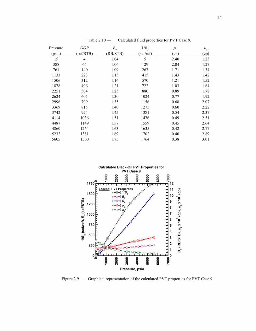
Table 2.10 — Calculated fluid properties for PVT Case 9.
Pressure GOR Bo 1/Bg o g (psia) (scf/STB) (RB/STB) (scf/rcf) (cp) (cp)
15 4 1.04 5 2.40 1.23 388 64 1.06 129 2.04 1.27 761 140 1.09 267 1.71 1.34
1133 223 1.13 415 1.43 1.42 1506 312 1.16 570 1.21 1.52 1878 406 1.21 722 1.03 1.64 2251 504 1.25 880 0.89 1.78 2624 605 1.30 1024 0.77 1.92 2996 709 1.35 1156 0.68 2.07 3369 815 1.40 1275 0.60 2.22 3742 924 1.45 1381 0.54 2.37 4114 1036 1.51 1476 0.49 2.51 4487 1149 1.57 1559 0.45 2.64 4860 1264 1.63 1635 0.42 2.77 5232 1381 1.69 1702 0.40 2.89 5605 1500 1.75 1764 0.38 3.01
Figure 2.9 — Graphical representation of the calculated PVT properties for PVT Case 9.

25
2.4 Relative Permeability Curves
The Corey-Brookes [CMG (software)] model for relative permeability curves was used to generate 13 sets
of relative permeability curves. The variables to generate these curves included the initial water saturation
(Swi), the Corey exponent (nCorey) for all phases and; the end points. For all relative permeability curves it
is assumed that the gas critical saturation is zero (Sgc = 0).
The Corey-Brookes model is given by10:
S oirwS wcrit
S wcritS wnw
k rwirok rw 1.......................................................................................................... (2.1)
S orwS wcon
S orwS onow
k rocwk row 1........................................................................................................ (2.2)
S orgS gcon
S orgS lnog
k roqcgk rog 1....................................................................................................... .(2.3)
S oirgS gcrit
S gcritS gn g
k roqclk rog 1......................................................................................................... (2.4)
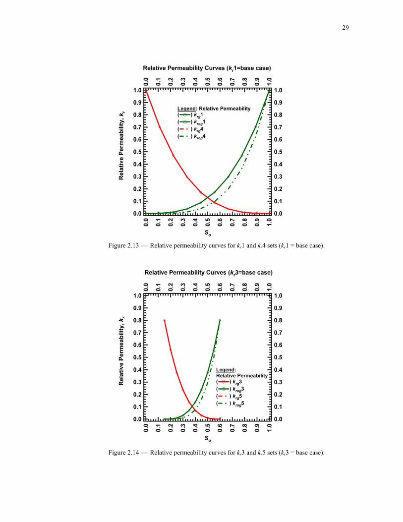
A total of 13 sets of relative permeability curves were generated using these formulas. For the purposes of
identification they are numbered 1 to 13 i.e. kr1, kr2, etc. The main group corresponds to kr1, kr2 and kr3
and; from these 3 sets all of the others were generated by varying either the Corey exponents or the end
points.
kr1, kr2 and kr3 correspond to the base case, the Corey exponent for all phases is equal to 3.
kr4 and kr5 are equivalent to kr1 and kr3 with a Corey oil exponent of 4 and all the remaining
exponents equal to 3.
kr6 to kr8 reproduce kr1, kr2 and kr3 with a Corey exponent of 2 for all phases.
kr9 to kr11 reproduce kr1, kr2 and kr3 with a Corey oil exponent of 4 for all phases.
kr12 and kr13 have the same Corey exponents as kr1, kr2 and kr3 but with either different end
points or initial saturations.
Table 2.11 to Table 2.13 shows a summary of the parameters employed to create each set of relative
permeability curves, sets are numbered 1 to 13 (i.e. kr1, kr2, etc):

26
Table 2.11 — Parameters used to for relative permeability curves calculation (kr1 to kr5).
Parameter kr1 kr2 kr3 kr4 kr5 Swcon 0 0.2 0.4 0 0.4 Swcrit 0 0.2 0.4 0 0.4 Soirw 0 0.15 0.25 0 0.25 Sorw 0 0.15 0.25 0 0.25 Soirg 0 0.1 0.15 0 0.15 Sorg 0 0.1 0.15 0 0.15 Sgcon 0 0 0 0 0 Sgcrit 0 0 0 0 0 krocw 1 0.9 0.8 1 0.8 krwiro 1 0.9 0.8 1 0.8 krgcl 1 0.9 0.8 1 0.8 krogcg 1 0.9 0.8 1 0.8
nw 3 3 3 3 3 now 3 3 3 3 3 nog 3 3 3 4 4 ng 3 3 3 3 3
Table 2.12 — Parameters used to for relative permeability curves calculation (kr6 to kr10).
Parameter kr6 kr7 kr8 kr9 kr10 Swcon 0 0.2 0.4 0 0.2 Swcrit 0 0.2 0.4 0 0.2 Soirw 0 0.15 0.25 0 0.15 Sorw 0 0.15 0.25 0 0.15 Soirg 0 0.1 0.15 0 0.1 Sorg 0 0.1 0.15 0 0.1 Sgcon 0 0 0 0 0 Sgcrit 0 0 0 0 0 krocw 1 0.9 0.8 1 0.9 krwiro 1 0.9 0.8 1 0.9 krgcl 1 0.9 0.8 1 0.9 krogcg 1 0.9 0.8 1 0.9
nw 2 2 2 4 4 now 2 2 2 4 4 nog 2 2 2 4 4 ng 2 2 2 4 4

27
Table 2.13 — Parameters used to for relative permeability curves calculation (kr11 to kr13).
Parameter kr11 kr12 kr13 Swcon 0.4 0.1 0.2 Swcrit 0.4 0.1 0.2 Soirw 0.25 0 0.15 Sorw 0.25 0 0.15 Soirg 0.15 0 0.1 Sorg 0.15 0 0.1 Sgcon 0 0 0 Sgcrit 0 0 0 krocw 0.8 0.9 0.7 krwiro 0.8 0.9 0.7 krgcl 0.8 0.9 0.7 krogcg 0.8 0.9 0.7
nw 4 3 3 now 4 3 3 nog 4 3 3 ng 4 3 3
Fig. 2.10 to Fig. 2.16 show the graphical representation of each relative permeability set alongside with
the modify sets, the reduction on relative permeability due to the change of end point, Corey exponent,
etc, can be observed:
Figure 2.10 — Relative permeability curves for kr1, kr6 and kr9 sets (kr1 = base case).

28
Figure 2.11 — Relative permeability curves for kr2, kr7 and kr10 sets (kr2 = base case).
Figure 2.12 — Relative permeability curves for kr3, kr8 and kr11 sets (kr3 = base case).
29
Figure 2.13 — Relative permeability curves for kr1 and kr4 sets (kr1 = base case).
Figure 2.14 — Relative permeability curves for kr3 and kr5 sets (kr3 = base case).

30
Figure 2.15 — Relative permeability curves for kr12 set.
Figure 2.16 — Relative permeability curves for kr13 set.

31
CHAPTER III
CORRELATION OF THE CHARACTERISTIC BEHAVIOR OF
SOLUTION-GAS-DRIVE RESERVOIRS
3.1. Correlation of the -parameter
Our correlation for the -parameter relation is "erf-based" and is given as:
ngnnn
BpkSTAPIGOR
Aog
Aow
Aw
A
oiA
oiA
oiA
iA
rogA
oiA
resAAA
13121110
987654321 )(1erf
........................................(3.1)
The coefficients for Eq. 3.1 are calibrated using a regression procedure and, are given in Table 3.1.
Table 3.1 — Constants for Eq. 3.1. Coefficients Value Coefficients Value
1 4.9734 A7 4.0536 A1 2.0369 A8 -0.0442 A2 -4.7583 A9 -0.1305 A3 -0.3713 A10 -0.0378 A4 0.3970 A11 -0.0006 A5 0.0922 A12 -0.1077 A6 -0.0053 A13 -0.0003

32
Figure 3.1 — Computed -parameter versus measured -parameter (all data). In Fig. 3.1 we present the "summary" correlation plot where the -parameter computed using the global
correlation is plotted versus the "base" or "measured" values of the -parameter as prescribed in Step 2.
The comparison shown in Fig. 3.1 suggests that we have achieved a fairly strong correlation of the -
parameter, with deviation from the perfect trend worsening as values of the -parameter increase.
3.2. Validation of the -parameter Correlation
A suit of correlation plots is proposed for the validation of the -parameter correlation. The proposed
plotting functions are illustrated for "Case 1" in Figs. 3.2-3.6. Fig. 3.2 is cast using the variables "1-
Normalized Mobility Function" and "Normalized Pressure Function" which are given in Eq. 1.17. The
use of these variable permits a "non-dimensional" view of the data and model functions. In Fig. 3.2 we
note the "local" best fit in red, and the global correlation fit in green — for this particular case the model
matches are in very close agreement; suggesting that the "global" correlation represents this particular
case (i.e., combination of variables) quite well. Obviously, this case was selected for the clarity it
provides, but it can also be considered to be a "typical" case in this work.
33
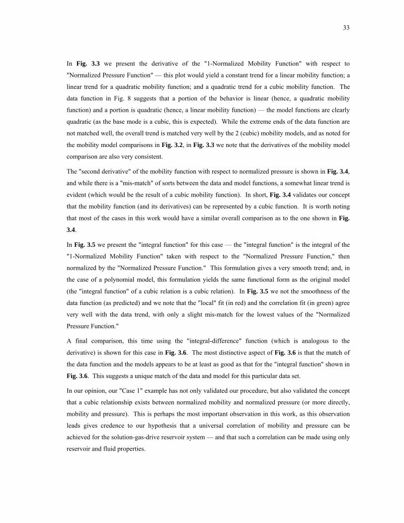
In Fig. 3.3 we present the derivative of the "1-Normalized Mobility Function" with respect to
"Normalized Pressure Function" — this plot would yield a constant trend for a linear mobility function; a
linear trend for a quadratic mobility function; and a quadratic trend for a cubic mobility function. The
data function in Fig. 8 suggests that a portion of the behavior is linear (hence, a quadratic mobility
function) and a portion is quadratic (hence, a linear mobility function) — the model functions are clearly
quadratic (as the base mode is a cubic, this is expected). While the extreme ends of the data function are
not matched well, the overall trend is matched very well by the 2 (cubic) mobility models, and as noted for
the mobility model comparisons in Fig. 3.2, in Fig. 3.3 we note that the derivatives of the mobility model
comparison are also very consistent.
The "second derivative" of the mobility function with respect to normalized pressure is shown in Fig. 3.4,
and while there is a "mis-match" of sorts between the data and model functions, a somewhat linear trend is
evident (which would be the result of a cubic mobility function). In short, Fig. 3.4 validates our concept
that the mobility function (and its derivatives) can be represented by a cubic function. It is worth noting
that most of the cases in this work would have a similar overall comparison as to the one shown in Fig.
3.4.
In Fig. 3.5 we present the "integral function" for this case — the "integral function" is the integral of the
"1-Normalized Mobility Function" taken with respect to the "Normalized Pressure Function," then
normalized by the "Normalized Pressure Function." This formulation gives a very smooth trend; and, in
the case of a polynomial model, this formulation yields the same functional form as the original model
(the "integral function" of a cubic relation is a cubic relation). In Fig. 3.5 we not the smoothness of the
data function (as predicted) and we note that the "local" fit (in red) and the correlation fit (in green) agree
very well with the data trend, with only a slight mis-match for the lowest values of the "Normalized
Pressure Function."
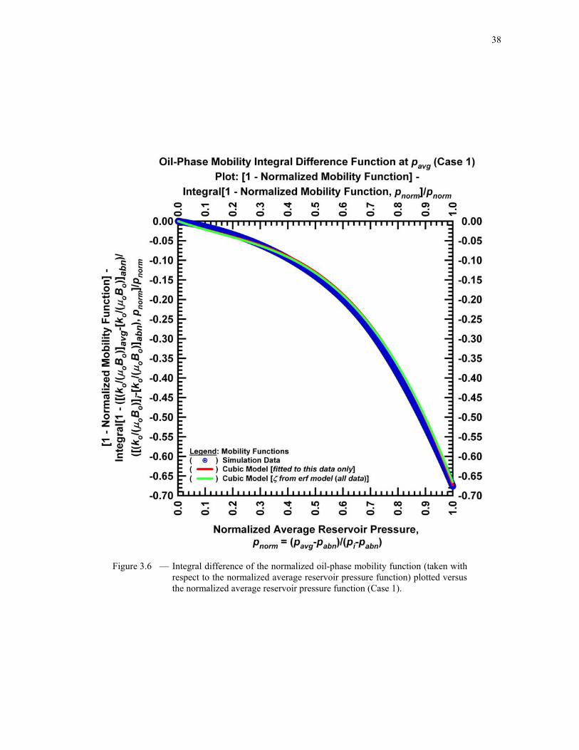
A final comparison, this time using the "integral-difference" function (which is analogous to the
derivative) is shown for this case in Fig. 3.6. The most distinctive aspect of Fig. 3.6 is that the match of
the data function and the models appears to be at least as good as that for the "integral function" shown in
Fig. 3.6. This suggests a unique match of the data and model for this particular data set.
In our opinion, our "Case 1" example has not only validated our procedure, but also validated the concept
that a cubic relationship exists between normalized mobility and normalized pressure (or more directly,
mobility and pressure). This is perhaps the most important observation in this work, as this observation
leads gives credence to our hypothesis that a universal correlation of mobility and pressure can be
achieved for the solution-gas-drive reservoir system — and that such a correlation can be made using only
reservoir and fluid properties.

34
Figure 3.2 — Normalized oil-phase mobility function plotted versus the normalized average reservoir pressure function (Case 1).

35
Figure 3.3 — Derivative of the normalized oil-phase mobility function (taken with respect to the normalized average reservoir pressure function) plotted versus the normalized average reservoir pressure function (Case 1).

36
Figure 3.4 — Second derivative of the normalized oil-phase mobility function (taken with respect to the normalized average reservoir pressure function) plotted versus the normalized average reservoir pressure function (Case 1).

37
Figure 3.5 — Integral of the normalized oil-phase mobility function (taken with respect to the normalized average reservoir pressure function) plotted versus the normalized average reservoir pressure function (Case 1).
38
Figure 3.6 — Integral difference of the normalized oil-phase mobility function (taken with respect to the normalized average reservoir pressure function) plotted versus the normalized average reservoir pressure function (Case 1).

39
3.3. Effect of Input Variables on the -parameter Correlation
A set of plots was developed to graphically assess the effect of the input variables on the -parameter
calculations. Figures 3.7 to 3.11 present the correlated -parameter computed using the global correlation
versus the "base" or "measured" values of the -parameter as a function of a particular input variable (e.g.,
GOR, API, TRes, oi, nw, ng, and nCorey).
In Fig. 3.7 we present the variation of the -parameter as a function of specified ranges of the GOR and
API variables — and we note that there is a slight increase in deviation from the perfect trend for the -
parameter, for > 0.6. This behavior could be attributed to a relatively smaller sample of data for these
ranges of the GOR and API variables, this is the most likely scenario.
Figure 3.7 — Effect of the GOR and API on the computed -parameter.
40
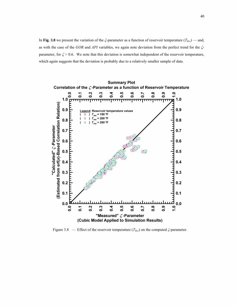
In Fig. 3.8 we present the variation of the -parameter as a function of reservoir temperature (TRes) — and,
as with the case of the GOR and API variables, we again note deviation from the perfect trend for the -
parameter, for > 0.6. We note that this deviation is somewhat independent of the reservoir temperature,
which again suggests that the deviation is probably due to a relatively smaller sample of data.
Figure 3.8 — Effect of the reservoir temperature (TRes) on the computed -parameter.

41
In Fig. 3.9 we present the variation of the -parameter as a function of initial oil mobility (oi). The
influence of oi is very similar to that for TRes — i.e., the outliers include data from each range of the oi-
parameter. This behavior (again) suggests that the deviation may be due to sample size.
Figure 3.9 — Effect of the initial oil mobility (oi) on the computed -parameter.

42
In Fig. 3.10 we present the variation of the -parameter as a function of Corey exponents for the water and
gas relative permeabilities (nw and ng). The influence of nw and ng does not cause significant deviation
from the perfect trend, except for the case of nw=ng=2. For the case of nw=ng=2, there is systematic
deviation in the computed versus measured -parameter values. It is our contention that this case
(nw=ng=2) is not necessarily unique, but most likely this deviation is caused by a low sample size for the
nw=ng=2 case.
Figure 3.10 — Effect of the Corey exponents for the water and gas relative permeabili-ties (nw and ng) on the computed -parameter.

43
In Fig. 3.11 we present the final sensitivity case, where the variation of the -parameter is considered as a
function of the Corey exponents for the oil relative permeability held constant (nog=now). The influence
of nog and now does not cause significant deviation from the perfect trend, similar to the cases where
nw=ng. Similar to the cases where nw=ng=2, for now=nog=2 there is (again) a systematic deviation in the
computed versus measured -parameter values. Similar to the nw=ng=2 cases, we also believe that the
influence exhibited by the now=nog=2 cases is due to the relatively small sample size.
The phenomena exhibited by the nw=ng=now=nog=2 cases is a point for future investigation.
Figure 3.11 — Effect of the Corey exponents for the oil relative permeabilities (nog and now) on the computed -parameter.

44
CHAPTER IV
CONCLUSIONS AND RECOMMENDATIONS
4.1. Conclusions
● The oil mobility profile can be uniquely approximated as a function of the correlating "-parameter,"
where the -parameter is a function of rock-fluid properties for p < pb.
● The simulation results confirm that the mobility profile is independent of the depletion mechanism
for a given set of rock-fluid conditions.
● The evaluation of the -parameter indicates a strong dependency on the Corey exponent (relative
permeability model).
● The development of validation plots confirm the concept that a cubic relationship exists between
normalized mobility and normalized pressure (or more directly, mobility and pressure).
● The established relationship between mobility and pressure indicate that a universal correlation of
mobility and pressure can be achieved for the solution-gas-drive reservoir system — and that such a
correlation can be made using only reservoir and fluid properties.
● The cubic polynomial based on the -parameter works well for all Corey exponent cases, except
nCorey=2.
4.2. Recommendations for Future Research
● The cubic -parameter model should be tested to validate the quartic "Vogel-form" IPR proposed by
Ilk et al. (2007) (these 2 relations are interrelated).
● The behavior of the -parameter with respect to the case of nCorey = 2 should be investigated further.
● The behavior of the -parameter was NOT evaluated against the following factors:
— skin effect — partial penetration — slanted/horizontal well — permeability anisotropy
A more extensive validation of the -parameter should be performed against these factors.
45
NOMENCLATURE
Variables
a = Constant established from the presumed behavior of the mobility profile.
API = API density of the oil
b = Constant established from the presumed behavior of the mobility profile.
bpss = Pseudosteady-state flow constant.
Bg = Gas formation volume factor, RB/SCF
Bo = Oil formation volume factor, RB/STB
Boi = Initial Oil formation volume factor, RB/STB
°F = Temperature, degree Fahrenheit
GORi = Initial Gas to Oil ratio, SCF/STB
h = Pay thickness, ft
Jo = Productivity index, STB/D/PSI
k = Absolute permeability, md
krocw = kro at connate Sw (Swcon)
krwiro = krw at irreducible So (Soirw)
krgcl = krg at connate Sl
krogcg = krog at connate Sg (Sgcon)
N = Original oil-in-place, MMSTB
Np = Cumulative oil production, STB
Np/N = Recovery, oil depletion ratio, fraction
nCorey= Corey exponent for relative permeability curves, dimensionless
nw = Exponent for calculating krw from krwiro, dimensionless
now = Exponent for calculating krow from krocw, dimensionless
nog = Exponent for calculating krog from krogcg, dimensionless
ng = Exponent for calculating krg from krgcl, dimensionless
p = Average reservoir pressure, psia
pabn = Abandonment pressure, psia
pbase = Base pressure, psia
pD,IPR = Dimensionless pressure
pn = Reference pressure, psia

46
pi = Initial reservoir pressure, psia
ppo = Oil pseudopressure, psia
pwf = Flowing bottomhole pressure, psia
qo = Oil flowrate, STB/D
qoi = Initial Oil flowrate, STB/D
qo,max = Maximum Oil flowrate, STB/D
Rso = Solution gas-oil ratio, SCF/STB
re = Outer reservoir radius, ft
rw = Wellbore radius, ft
s = Skin factor, dimensionless
Sg = Gas saturation, dimensionless
So = Oil saturation, dimensionless
Swcon = Endpoint Saturation: Connate Water
Swcrit = Endpoint Saturation: Critical Water
Soirw = Endpoint Saturation: Irreducible Oil (w/water)
Sorw = Endpoint Saturation: Residual Oil (w/water)
Soirg = Endpoint Saturation: Irreducible Oil (w/gas)
Sorg = Endpoint Saturation: Residual Oil (w/gas)
Sgcon = Endpoint Saturation: Connate Gas
Sgcrit = Endpoint Saturation: Critical Gas
TRes = Reservoir temperature, Deg F
Greek Symbols
= Porosity, fraction
= General IPR "lump" parameter, dimensionless
= Linear IPR "lump" parameter, dimensionless
= General IPR "lump" parameter, dimensionless
= Mobility function, md/(cp-RB/STB)
D,IPR = Dimensionless oil mobility, dimensionless
g = Gas viscosity, cp
o = Oil viscosity, cp
= General IPR "lump" parameter, dimensionless
= General IPR "lump" parameter, dimensionless
= Characteristic mobility parameter, dimensionless
47
REFERENCES
Camacho-V, R.G. and Raghavan, R.: "Inflow Performance Relationships for Solution Gas-Drive
Reservoirs," JPT (May 1989) 541-550.
CMG (software) Version 2800.10.3118.22139, Computer Modeling Group Ltd, Canada (2008)
Del Castillo, Y.: "New Perspectives on Vogel-Type IPR Models for Gas Condensate and Solution
Gas-Drive Systems", M.S. Thesis, Texas A&M U., August 2003, College Station, TX.
Economides, M.J., Hill, A.D., Ehlig-Economides, C.: "Petroleum Production Systems". Prentice
Hall Petroleum Engineering Series (1994), 22-23.
Fetkovich, M.J.: "The Isochronal Testing of Oil Wells," paper SPE 4529 presented at the SPE
Annual Fall Meeting held in Las Vegas, Nevada, U.S.A., 30 September – 03 October 1973.
Rawlins, E.L. and Schellhardt, M.A.: Backpressure Data on Natural Gas Wells and Their
Application to Production Practices, Monograph Series, USBM (1935) 7.
Richardson, J.M. and Shaw A.H: "Two-Rate IPR Testing — A Practical Production Tool," JCPT,
(March-April 1982) 57-61.
Vogel, J. V.: "Inflow Performance Relationships for Solution-Gas Drive Wells," JPT (Jan. 1968)
83-92.
Wiggins, M.L., Russell, J.E., Jennings, J.W.: "Analytical Development of Vogel-Type Inflow
Performance Relationships," SPE Journal (December 1996) 355-362.

48
APPENDIX A
DEFINITION OF THE -CHARACTERISTIC FUNCTION (CUBIC MODEL)
In this Appendix we present an inventory of the relations for the "characteristic" (ζ-parameter)
formulation proposed by Ilk, et al [2007] is given as:
32
)1(2 )1( 1 )](/[)](/[
)](/[)](/[ 1
abni
abn
abni
abn
abni
abn
abnpoooipooo
abnpooopooo
pp
pp
pp
pp
pp
pp
BkBk
BkBk
(where ζ < 1) ............................................................................................................................................(A-1)
Plotting Function (PF1): (base function)
abni
abn
abnpoooipooo
abnpooopooo
pp
pp
BkBk
BkBk versus
)](/[)](/[
)](/[)](/[ 1
..................................................................(A-2)
Plotting Function (PF2): (first derivative function)
abni
abn
abni
abn
abnpoooipooo
abnpooopooo
pp
pp
pp
ppd
BkBk
BkBkd versus/
)](/[)](/[
)](/[)](/[ 1
.........................................(A-3)
Plotting Function (PF3): (second derivative function)
abni
abn
abni
abn
abnpoooipooo
abnpooopooo
pp
pp
pp
ppd
BkBk
BkBkd versus/
)](/[)](/[
)](/[)](/[ 1
22
.....................................(A-4)
Plotting Function (PF4): (integral function)
abni
abn
normp
abnpoooipooo
abnpooopooo
norm pp
pp
BkBk
BkBk
p versus
)](/[)](/[
)](/[)](/[ 1
1
0
..............................................(A-5)
Plotting Function (PF5): (integral-difference function)
abni
abn
normp
abnpoooipooo
abnpooopooo
norm
abnpoooipooo
abnpooopooo
pp
pp
BkBk
BkBk
p
BkBk
BkBk
versus)](/[)](/[
)](/[)](/[ 1
1
)](/[)](/[
)](/[)](/[ 1
0
.............................(A-6)

49
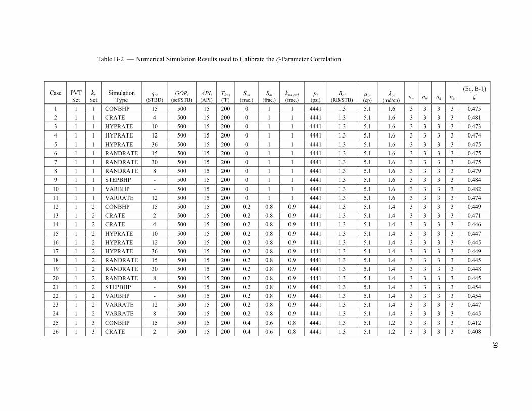
APPENDIX B
NUMERICAL SIMULATION RESULTS USED TO CALIBRATE THE -
PARAMETER CORRELATION
In this Appendix we provide a summary of the numerical simulation results used to calibrate the -
parameter correlation. The input data parameters for this work are given in Table B-1 and the results of
this simulation study are provided in Table B-2. Our defining (or "local") model in a cubic form for the
-parameter is given as:
32
)1(2 )1( 1 )](/[)](/[
)](/[)](/[ 1
abni
abn
abni
abn
abni
abn
abnpoooipooo
abnpooopooo
pp
pp
pp
pp
pp
pp
BkBk
BkBk
(where ζ < 1) ............................................................................................................................................ (B-1)
We also develop an empirical correlation of for the -parameter, the form of this correlation is given by:
ngnnn
BpkSTAPIGOR
Aog
Aow
Aw
A
oiA
oiA
oiA
iA
rogA
oiA
resAAA
13121110
987654321 1)(1erf
..................................... (B-2)
The coefficients in Eq. B-2 are derived using the values given in the results table provided later in this
Appendix.
Table B-1 — Input Parameters for the Numerical Simulation Study
GORi
(scf/STB) APIi
(Deg API) TRes
(Deg F) Swi
(fraction)Soi
(fraction)kr, end
(dimensionless) nCorey
(dimensionless)500 15 150 0 1 0.7 2 1000 25 200 0.1 0.9 0.8 3 1500 35 250 0.2 0.8 0.9 4
- - - 0.4 0.6 1
50
Table B-2 — Numerical Simulation Results used to Calibrate the -Parameter Correlation
Case
PVT Set
kr
Set
Simulation
Type
qoi
(STBD)
GORi
(scf/STB)
APIi (API)
TRes (oF)
Swi
(frac.)
Soi
(frac.)
kro,end (frac.)
pi
(psi)
Boi
(RB/STB)
oi (cp)
oi
(md/cp)
nw
nw
ng
ng
(Eq. B-1)
1 1 1 CONBHP 15 500 15 200 0 1 1 4441 1.3 5.1 1.6 3 3 3 3 0.475
2 1 1 CRATE 4 500 15 200 0 1 1 4441 1.3 5.1 1.6 3 3 3 3 0.481
3 1 1 HYPRATE 10 500 15 200 0 1 1 4441 1.3 5.1 1.6 3 3 3 3 0.473
4 1 1 HYPRATE 12 500 15 200 0 1 1 4441 1.3 5.1 1.6 3 3 3 3 0.474
5 1 1 HYPRATE 36 500 15 200 0 1 1 4441 1.3 5.1 1.6 3 3 3 3 0.475
6 1 1 RANDRATE 15 500 15 200 0 1 1 4441 1.3 5.1 1.6 3 3 3 3 0.475
7 1 1 RANDRATE 30 500 15 200 0 1 1 4441 1.3 5.1 1.6 3 3 3 3 0.475
8 1 1 RANDRATE 8 500 15 200 0 1 1 4441 1.3 5.1 1.6 3 3 3 3 0.479
9 1 1 STEPBHP - 500 15 200 0 1 1 4441 1.3 5.1 1.6 3 3 3 3 0.484
10 1 1 VARBHP - 500 15 200 0 1 1 4441 1.3 5.1 1.6 3 3 3 3 0.482
11 1 1 VARRATE 12 500 15 200 0 1 1 4441 1.3 5.1 1.6 3 3 3 3 0.474
12 1 2 CONBHP 15 500 15 200 0.2 0.8 0.9 4441 1.3 5.1 1.4 3 3 3 3 0.449
13 1 2 CRATE 2 500 15 200 0.2 0.8 0.9 4441 1.3 5.1 1.4 3 3 3 3 0.471
14 1 2 CRATE 4 500 15 200 0.2 0.8 0.9 4441 1.3 5.1 1.4 3 3 3 3 0.446
15 1 2 HYPRATE 10 500 15 200 0.2 0.8 0.9 4441 1.3 5.1 1.4 3 3 3 3 0.447
16 1 2 HYPRATE 12 500 15 200 0.2 0.8 0.9 4441 1.3 5.1 1.4 3 3 3 3 0.445
17 1 2 HYPRATE 36 500 15 200 0.2 0.8 0.9 4441 1.3 5.1 1.4 3 3 3 3 0.449
18 1 2 RANDRATE 15 500 15 200 0.2 0.8 0.9 4441 1.3 5.1 1.4 3 3 3 3 0.445
19 1 2 RANDRATE 30 500 15 200 0.2 0.8 0.9 4441 1.3 5.1 1.4 3 3 3 3 0.448
20 1 2 RANDRATE 8 500 15 200 0.2 0.8 0.9 4441 1.3 5.1 1.4 3 3 3 3 0.445
21 1 2 STEPBHP - 500 15 200 0.2 0.8 0.9 4441 1.3 5.1 1.4 3 3 3 3 0.454
22 1 2 VARBHP - 500 15 200 0.2 0.8 0.9 4441 1.3 5.1 1.4 3 3 3 3 0.454
23 1 2 VARRATE 12 500 15 200 0.2 0.8 0.9 4441 1.3 5.1 1.4 3 3 3 3 0.447
24 1 2 VARRATE 8 500 15 200 0.2 0.8 0.9 4441 1.3 5.1 1.4 3 3 3 3 0.445
25 1 3 CONBHP 15 500 15 200 0.4 0.6 0.8 4441 1.3 5.1 1.2 3 3 3 3 0.412
26 1 3 CRATE 2 500 15 200 0.4 0.6 0.8 4441 1.3 5.1 1.2 3 3 3 3 0.408

51
Case
PVT Set
kr
Set
Simulation
Type
qoi
(STBD)
GORi
(scf/STB)
APIi (API)
TRes (oF)
Swi
(frac.)
Soi
(frac.)
kro,end (frac.)
pi
(psi)
Boi
(RB/STB)
oi (cp)
oi
(md/cp)
nw
nw
ng
ng
(Eq. B-1)
27 1 3 CRATE 4 500 15 200 0.4 0.6 0.8 4441 1.3 5.1 1.2 3 3 3 3 0.405
28 1 3 HYPRATE 10 500 15 200 0.4 0.6 0.8 4441 1.3 5.1 1.2 3 3 3 3 0.409
29 1 3 HYPRATE 12 500 15 200 0.4 0.6 0.8 4441 1.3 5.1 1.2 3 3 3 3 0.408
30 1 3 HYPRATE 36 500 15 200 0.4 0.6 0.8 4441 1.3 5.1 1.2 3 3 3 3 0.412
31 1 3 RANDRATE 15 500 15 200 0.4 0.6 0.8 4441 1.3 5.1 1.2 3 3 3 3 0.407
32 1 3 RANDRATE 30 500 15 200 0.4 0.6 0.8 4441 1.3 5.1 1.2 3 3 3 3 0.410
33 1 3 RANDRATE 8 500 15 200 0.4 0.6 0.8 4441 1.3 5.1 1.2 3 3 3 3 0.405
34 1 3 STEPBHP - 500 15 200 0.4 0.6 0.8 4441 1.3 5.1 1.2 3 3 3 3 0.415
35 1 3 VARBHP - 500 15 200 0.4 0.6 0.8 4441 1.3 5.1 1.2 3 3 3 3 0.417
36 1 3 VARRATE 12 500 15 200 0.4 0.6 0.8 4441 1.3 5.1 1.2 3 3 3 3 0.409
37 1 3 VARRATE 8 500 15 200 0.4 0.6 0.8 4441 1.3 5.1 1.2 3 3 3 3 0.407
38 1 4 CONBHP 15 500 15 200 0 1 1 4441 1.3 5.1 1.6 3 3 4 3 0.403
39 1 4 CRATE 4 500 15 200 0 1 1 4441 1.3 5.1 1.6 3 3 4 3 0.408
40 1 4 HYPRATE 10 500 15 200 0 1 1 4441 1.3 5.1 1.6 3 3 4 3 0.401
41 1 4 HYPRATE 12 500 15 200 0 1 1 4441 1.3 5.1 1.6 3 3 4 3 0.401
42 1 4 HYPRATE 36 500 15 200 0 1 1 4441 1.3 5.1 1.6 3 3 4 3 0.403
43 1 4 RANDRATE 15 500 15 200 0 1 1 4441 1.3 5.1 1.6 3 3 4 3 0.402
44 1 4 RANDRATE 30 500 15 200 0 1 1 4441 1.3 5.1 1.6 3 3 4 3 0.402
45 1 4 RANDRATE 8 500 15 200 0 1 1 4441 1.3 5.1 1.6 3 3 4 3 0.406
46 1 4 STEPBHP - 500 15 200 0 1 1 4441 1.3 5.1 1.6 3 3 4 3 0.411
47 1 4 VARBHP - 500 15 200 0 1 1 4441 1.3 5.1 1.6 3 3 4 3 0.409
48 1 4 VARRATE 12 500 15 200 0 1 1 4441 1.3 5.1 1.6 3 3 4 3 0.400
49 1 5 CONBHP 15 500 15 200 0.4 0.6 0.8 4441 1.3 5.1 1.2 3 3 4 3 0.326
50 1 5 CRATE 2 500 15 200 0.4 0.6 0.8 4441 1.3 5.1 1.2 3 3 4 3 0.323
51 1 5 CRATE 4 500 15 200 0.4 0.6 0.8 4441 1.3 5.1 1.2 3 3 4 3 0.322
52 1 5 HYPRATE 10 500 15 200 0.4 0.6 0.8 4441 1.3 5.1 1.2 3 3 4 3 0.326
53 1 5 HYPRATE 12 500 15 200 0.4 0.6 0.8 4441 1.3 5.1 1.2 3 3 4 3 0.324
54 1 5 HYPRATE 36 500 15 200 0.4 0.6 0.8 4441 1.3 5.1 1.2 3 3 4 3 0.326
55 1 5 RANDRATE 15 500 15 200 0.4 0.6 0.8 4441 1.3 5.1 1.2 3 3 4 3 0.324
56 1 5 RANDRATE 30 500 15 200 0.4 0.6 0.8 4441 1.3 5.1 1.2 3 3 4 3 0.325

52
Case
PVT Set
kr
Set
Simulation
Type
qoi
(STBD)
GORi
(scf/STB)
APIi (API)
TRes (oF)
Swi
(frac.)
Soi
(frac.)
kro,end (frac.)
pi
(psi)
Boi
(RB/STB)
oi (cp)
oi
(md/cp)
nw
nw
ng
ng
(Eq. B-1)
57 1 5 RANDRATE 8 500 15 200 0.4 0.6 0.8 4441 1.3 5.1 1.2 3 3 4 3 0.322
58 1 5 STEPBHP - 500 15 200 0.4 0.6 0.8 4441 1.3 5.1 1.2 3 3 4 3 0.330
59 1 5 VARBHP - 500 15 200 0.4 0.6 0.8 4441 1.3 5.1 1.2 3 3 4 3 0.330
60 1 5 VARRATE 12 500 15 200 0.4 0.6 0.8 4441 1.3 5.1 1.2 3 3 4 3 0.325
61 1 5 VARRATE 8 500 15 200 0.4 0.6 0.8 4441 1.3 5.1 1.2 3 3 4 3 0.323
62 1 6 CONBHP 15 500 15 200 0 1 1 4441 1.3 5.1 1.6 2 2 2 2 0.597
63 1 6 CRATE 4 500 15 200 0 1 1 4441 1.3 5.1 1.6 2 2 2 2 0.594
64 1 6 RANDRATE 8 500 15 200 0 1 1 4441 1.3 5.1 1.6 2 2 2 2 0.595
65 1 6 STEPBHP - 500 15 200 0 1 1 4441 1.3 5.1 1.6 2 2 2 2 0.595
66 1 6 VARBHP - 500 15 200 0 1 1 4441 1.3 5.1 1.6 2 2 2 2 0.603
67 1 6 VARRATE 12 500 15 200 0 1 1 4441 1.3 5.1 1.6 2 2 2 2 0.595
68 1 7 CONBHP 15 500 15 200 0.2 0.8 0.9 4441 1.3 5.1 1.4 2 2 2 2 0.632
69 1 7 CRATE 4 500 15 200 0.2 0.8 0.9 4441 1.3 5.1 1.4 2 2 2 2 0.629
70 1 7 STEPBHP - 500 15 200 0.2 0.8 0.9 4441 1.3 5.1 1.4 2 2 2 2 0.630
71 1 7 VARBHP - 500 15 200 0.2 0.8 0.9 4441 1.3 5.1 1.4 2 2 2 2 0.636
72 1 7 VARRATE 12 500 15 200 0.2 0.8 0.9 4441 1.3 5.1 1.4 2 2 2 2 0.631
73 1 8 CONBHP 15 500 15 200 0.4 0.6 0.8 4441 1.3 5.1 1.2 2 2 2 2 0.562
74 1 8 CRATE 4 500 15 200 0.4 0.6 0.8 4441 1.3 5.1 1.2 2 2 2 2 0.555
75 1 8 HYPRATE 13 500 15 200 0.4 0.6 0.8 4441 1.3 5.1 1.2 2 2 2 2 0.561
76 1 8 RANDRATE 10 500 15 200 0.4 0.6 0.8 4441 1.3 5.1 1.2 2 2 2 2 0.557
77 1 8 STEPBHP - 500 15 200 0.4 0.6 0.8 4441 1.3 5.1 1.2 2 2 2 2 0.559
78 1 8 VARBHP - 500 15 200 0.4 0.6 0.8 4441 1.3 5.1 1.2 2 2 2 2 0.565
79 1 8 VARRATE 12 500 15 200 0.4 0.6 0.8 4441 1.3 5.1 1.2 2 2 2 2 0.561
80 1 9 CONBHP 15 500 15 200 0 1 1 4441 1.3 5.1 1.6 4 4 4 4 0.366
81 1 9 CRATE 4 500 15 200 0 1 1 4441 1.3 5.1 1.6 4 4 4 4 0.378
82 1 9 HYPRATE 17 500 15 200 0 1 1 4441 1.3 5.1 1.6 4 4 4 4 0.366
83 1 9 STEPBHP - 500 15 200 0 1 1 4441 1.3 5.1 1.6 4 4 4 4 0.369
84 1 9 VARBHP - 500 15 200 0 1 1 4441 1.3 5.1 1.6 4 4 4 4 0.393
85 1 9 VARRATE 12 500 15 200 0 1 1 4441 1.3 5.1 1.6 4 4 4 4 0.381
86 1 10 CONBHP 15 500 15 200 0.2 0.8 0.9 4441 1.3 5.1 1.4 4 4 4 4 0.326
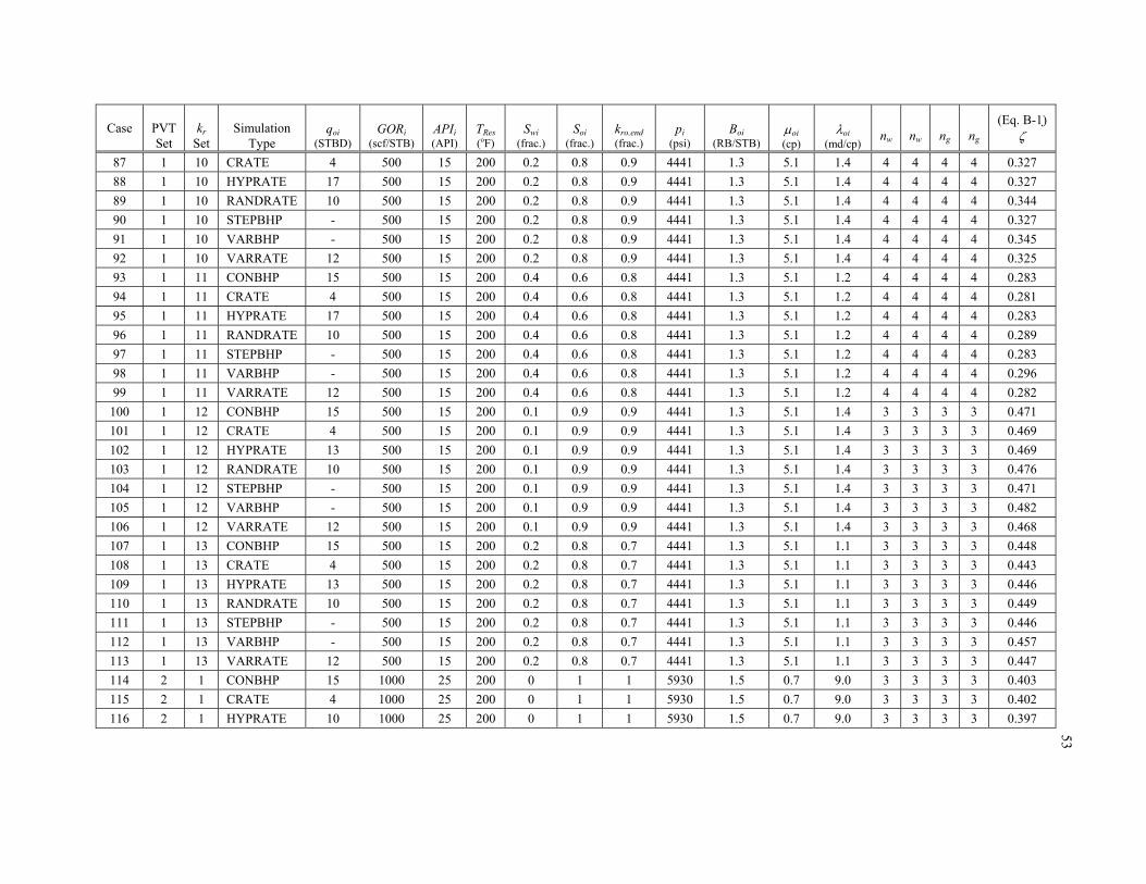
53
Case
PVT Set
kr
Set
Simulation
Type
qoi
(STBD)
GORi
(scf/STB)
APIi (API)
TRes (oF)
Swi
(frac.)
Soi
(frac.)
kro,end (frac.)
pi
(psi)
Boi
(RB/STB)
oi (cp)
oi
(md/cp)
nw
nw
ng
ng
(Eq. B-1)
87 1 10 CRATE 4 500 15 200 0.2 0.8 0.9 4441 1.3 5.1 1.4 4 4 4 4 0.327
88 1 10 HYPRATE 17 500 15 200 0.2 0.8 0.9 4441 1.3 5.1 1.4 4 4 4 4 0.327
89 1 10 RANDRATE 10 500 15 200 0.2 0.8 0.9 4441 1.3 5.1 1.4 4 4 4 4 0.344
90 1 10 STEPBHP - 500 15 200 0.2 0.8 0.9 4441 1.3 5.1 1.4 4 4 4 4 0.327
91 1 10 VARBHP - 500 15 200 0.2 0.8 0.9 4441 1.3 5.1 1.4 4 4 4 4 0.345
92 1 10 VARRATE 12 500 15 200 0.2 0.8 0.9 4441 1.3 5.1 1.4 4 4 4 4 0.325
93 1 11 CONBHP 15 500 15 200 0.4 0.6 0.8 4441 1.3 5.1 1.2 4 4 4 4 0.283
94 1 11 CRATE 4 500 15 200 0.4 0.6 0.8 4441 1.3 5.1 1.2 4 4 4 4 0.281
95 1 11 HYPRATE 17 500 15 200 0.4 0.6 0.8 4441 1.3 5.1 1.2 4 4 4 4 0.283
96 1 11 RANDRATE 10 500 15 200 0.4 0.6 0.8 4441 1.3 5.1 1.2 4 4 4 4 0.289
97 1 11 STEPBHP - 500 15 200 0.4 0.6 0.8 4441 1.3 5.1 1.2 4 4 4 4 0.283
98 1 11 VARBHP - 500 15 200 0.4 0.6 0.8 4441 1.3 5.1 1.2 4 4 4 4 0.296
99 1 11 VARRATE 12 500 15 200 0.4 0.6 0.8 4441 1.3 5.1 1.2 4 4 4 4 0.282
100 1 12 CONBHP 15 500 15 200 0.1 0.9 0.9 4441 1.3 5.1 1.4 3 3 3 3 0.471
101 1 12 CRATE 4 500 15 200 0.1 0.9 0.9 4441 1.3 5.1 1.4 3 3 3 3 0.469
102 1 12 HYPRATE 13 500 15 200 0.1 0.9 0.9 4441 1.3 5.1 1.4 3 3 3 3 0.469
103 1 12 RANDRATE 10 500 15 200 0.1 0.9 0.9 4441 1.3 5.1 1.4 3 3 3 3 0.476
104 1 12 STEPBHP - 500 15 200 0.1 0.9 0.9 4441 1.3 5.1 1.4 3 3 3 3 0.471
105 1 12 VARBHP - 500 15 200 0.1 0.9 0.9 4441 1.3 5.1 1.4 3 3 3 3 0.482
106 1 12 VARRATE 12 500 15 200 0.1 0.9 0.9 4441 1.3 5.1 1.4 3 3 3 3 0.468
107 1 13 CONBHP 15 500 15 200 0.2 0.8 0.7 4441 1.3 5.1 1.1 3 3 3 3 0.448
108 1 13 CRATE 4 500 15 200 0.2 0.8 0.7 4441 1.3 5.1 1.1 3 3 3 3 0.443
109 1 13 HYPRATE 13 500 15 200 0.2 0.8 0.7 4441 1.3 5.1 1.1 3 3 3 3 0.446
110 1 13 RANDRATE 10 500 15 200 0.2 0.8 0.7 4441 1.3 5.1 1.1 3 3 3 3 0.449
111 1 13 STEPBHP - 500 15 200 0.2 0.8 0.7 4441 1.3 5.1 1.1 3 3 3 3 0.446
112 1 13 VARBHP - 500 15 200 0.2 0.8 0.7 4441 1.3 5.1 1.1 3 3 3 3 0.457
113 1 13 VARRATE 12 500 15 200 0.2 0.8 0.7 4441 1.3 5.1 1.1 3 3 3 3 0.447
114 2 1 CONBHP 15 1000 25 200 0 1 1 5930 1.5 0.7 9.0 3 3 3 3 0.403
115 2 1 CRATE 4 1000 25 200 0 1 1 5930 1.5 0.7 9.0 3 3 3 3 0.402
116 2 1 HYPRATE 10 1000 25 200 0 1 1 5930 1.5 0.7 9.0 3 3 3 3 0.397

54
Case
PVT Set
kr
Set
Simulation
Type
qoi
(STBD)
GORi
(scf/STB)
APIi (API)
TRes (oF)
Swi
(frac.)
Soi
(frac.)
kro,end (frac.)
pi
(psi)
Boi
(RB/STB)
oi (cp)
oi
(md/cp)
nw
nw
ng
ng
(Eq. B-1)
117 2 1 HYPRATE 12 1000 25 200 0 1 1 5930 1.5 0.7 9.0 3 3 3 3 0.400
118 2 1 HYPRATE 23 1000 25 200 0 1 1 5930 1.5 0.7 9.0 3 3 3 3 0.396
119 2 1 RANDRATE 15 1000 25 200 0 1 1 5930 1.5 0.7 9.0 3 3 3 3 0.396
120 2 1 RANDRATE 20 1000 25 200 0 1 1 5930 1.5 0.7 9.0 3 3 3 3 0.396
121 2 1 RANDRATE 8 1000 25 200 0 1 1 5930 1.5 0.7 9.0 3 3 3 3 0.400
122 2 1 STEPBHP - 1000 25 200 0 1 1 5930 1.5 0.7 9.0 3 3 3 3 0.406
123 2 1 VARBHP - 1000 25 200 0 1 1 5930 1.5 0.7 9.0 3 3 3 3 0.406
124 2 1 VARRATE 12 1000 25 200 0 1 1 5930 1.5 0.7 9.0 3 3 3 3 0.400
125 2 2 CONBHP 15 1000 25 200 0.2 0.8 0.9 5930 1.5 0.7 8.1 3 3 3 3 0.362
126 2 2 CRATE 4 1000 25 200 0.2 0.8 0.9 5930 1.5 0.7 8.1 3 3 3 3 0.356
127 2 2 HYPRATE 10 1000 25 200 0.2 0.8 0.9 5930 1.5 0.7 8.1 3 3 3 3 0.355
128 2 2 HYPRATE 12 1000 25 200 0.2 0.8 0.9 5930 1.5 0.7 8.1 3 3 3 3 0.355
129 2 2 HYPRATE 23 1000 25 200 0.2 0.8 0.9 5930 1.5 0.7 8.1 3 3 3 3 0.355
130 2 2 RANDRATE 15 1000 25 200 0.2 0.8 0.9 5930 1.5 0.7 8.1 3 3 3 3 0.355
131 2 2 RANDRATE 20 1000 25 200 0.2 0.8 0.9 5930 1.5 0.7 8.1 3 3 3 3 0.355
132 2 2 RANDRATE 8 1000 25 200 0.2 0.8 0.9 5930 1.5 0.7 8.1 3 3 3 3 0.355
133 2 2 STEPBHP - 1000 25 200 0.2 0.8 0.9 5930 1.5 0.7 8.1 3 3 3 3 0.363
134 2 2 VARBHP - 1000 25 200 0.2 0.8 0.9 5930 1.5 0.7 8.1 3 3 3 3 0.364
135 2 2 VARRATE 12 1000 25 200 0.2 0.8 0.9 5930 1.5 0.7 8.1 3 3 3 3 0.355
136 2 2 VARRATE 8 1000 25 200 0.2 0.8 0.9 5930 1.5 0.7 8.1 3 3 3 3 0.357
137 2 3 CONBHP 15 1000 25 200 0.4 0.6 0.8 5930 1.5 0.7 7.2 3 3 3 3 0.317
138 2 3 CRATE 2 1000 25 200 0.4 0.6 0.8 5930 1.5 0.7 7.2 3 3 3 3 0.310
139 2 3 CRATE 4 1000 25 200 0.4 0.6 0.8 5930 1.5 0.7 7.2 3 3 3 3 0.309
140 2 3 HYPRATE 10 1000 25 200 0.4 0.6 0.8 5930 1.5 0.7 7.2 3 3 3 3 0.309
141 2 3 HYPRATE 12 1000 25 200 0.4 0.6 0.8 5930 1.5 0.7 7.2 3 3 3 3 0.309
142 2 3 HYPRATE 23 1000 25 200 0.4 0.6 0.8 5930 1.5 0.7 7.2 3 3 3 3 0.310
143 2 3 RANDRATE 15 1000 25 200 0.4 0.6 0.8 5930 1.5 0.7 7.2 3 3 3 3 0.309
144 2 3 RANDRATE 20 1000 25 200 0.4 0.6 0.8 5930 1.5 0.7 7.2 3 3 3 3 0.310
145 2 3 STEPBHP - 1000 25 200 0.4 0.6 0.8 5930 1.5 0.7 7.2 3 3 3 3 0.316
146 2 3 VARBHP - 1000 25 200 0.4 0.6 0.8 5930 1.5 0.7 7.2 3 3 3 3 0.317

55
Case
PVT Set
kr
Set
Simulation
Type
qoi
(STBD)
GORi
(scf/STB)
APIi (API)
TRes (oF)
Swi
(frac.)
Soi
(frac.)
kro,end (frac.)
pi
(psi)
Boi
(RB/STB)
oi (cp)
oi
(md/cp)
nw
nw
ng
ng
(Eq. B-1)
147 2 3 VARRATE 12 1000 25 200 0.4 0.6 0.8 5930 1.5 0.7 7.2 3 3 3 3 0.309
148 2 3 VARRATE 8 1000 25 200 0.4 0.6 0.8 5930 1.5 0.7 7.2 3 3 3 3 0.309
149 2 4 CONBHP 15 1000 25 200 0 1 1 5930 1.5 0.7 9.0 3 3 4 3 0.305
150 2 4 CRATE 4 1000 25 200 0 1 1 5930 1.5 0.7 9.0 3 3 4 3 0.302
151 2 4 HYPRATE 10 1000 25 200 0 1 1 5930 1.5 0.7 9.0 3 3 4 3 0.298
152 2 4 HYPRATE 12 1000 25 200 0 1 1 5930 1.5 0.7 9.0 3 3 4 3 0.299
153 2 4 HYPRATE 23 1000 25 200 0 1 1 5930 1.5 0.7 9.0 3 3 4 3 0.298
154 2 4 RANDRATE 15 1000 25 200 0 1 1 5930 1.5 0.7 9.0 3 3 4 3 0.298
155 2 4 RANDRATE 20 1000 25 200 0 1 1 5930 1.5 0.7 9.0 3 3 4 3 0.298
156 2 4 RANDRATE 8 1000 25 200 0 1 1 5930 1.5 0.7 9.0 3 3 4 3 0.301
157 2 4 STEPBHP - 1000 25 200 0 1 1 5930 1.5 0.7 9.0 3 3 4 3 0.307
158 2 4 VARBHP - 1000 25 200 0 1 1 5930 1.5 0.7 9.0 3 3 4 3 0.308
159 2 4 VARRATE 12 1000 25 200 0 1 1 5930 1.5 0.7 9.0 3 3 4 3 0.299
160 2 5 CONBHP 15 1000 25 200 0.4 0.6 0.8 5930 1.5 0.7 7.2 3 3 4 3 0.210
161 2 5 CRATE 2 1000 25 200 0.4 0.6 0.8 5930 1.5 0.7 7.2 3 3 4 3 0.205
162 2 5 CRATE 4 1000 25 200 0.4 0.6 0.8 5930 1.5 0.7 7.2 3 3 4 3 0.204
163 2 5 HYPRATE 10 1000 25 200 0.4 0.6 0.8 5930 1.5 0.7 7.2 3 3 4 3 0.205
164 2 5 HYPRATE 12 1000 25 200 0.4 0.6 0.8 5930 1.5 0.7 7.2 3 3 4 3 0.204
165 2 5 HYPRATE 23 1000 25 200 0.4 0.6 0.8 5930 1.5 0.7 7.2 3 3 4 3 0.205
166 2 5 RANDRATE 15 1000 25 200 0.4 0.6 0.8 5930 1.5 0.7 7.2 3 3 4 3 0.204
167 2 5 RANDRATE 20 1000 25 200 0.4 0.6 0.8 5930 1.5 0.7 7.2 3 3 4 3 0.205
168 2 5 RANDRATE 8 1000 25 200 0.4 0.6 0.8 5930 1.5 0.7 7.2 3 3 4 3 0.204
169 2 5 STEPBHP - 1000 25 200 0.4 0.6 0.8 5930 1.5 0.7 7.2 3 3 4 3 0.211
170 2 5 VARBHP - 1000 25 200 0.4 0.6 0.8 5930 1.5 0.7 7.2 3 3 4 3 0.211
171 2 5 VARRATE 12 1000 25 200 0.4 0.6 0.8 5930 1.5 0.7 7.2 3 3 4 3 0.205
172 2 5 VARRATE 8 1000 25 200 0.4 0.6 0.8 5930 1.5 0.7 7.2 3 3 4 3 0.204
173 2 6 CONBHP 15 1000 25 200 0 1 1 5930 1.5 0.7 9.0 2 2 2 2 0.572
174 2 6 CRATE 4 1000 25 200 0 1 1 5930 1.5 0.7 9.0 2 2 2 2 0.565
175 2 6 RANDRATE 8 1000 25 200 0 1 1 5930 1.5 0.7 9.0 2 2 2 2 0.565
176 2 6 STEPBHP - 1000 25 200 0 1 1 5930 1.5 0.7 9.0 2 2 2 2 0.567

56
Case
PVT Set
kr
Set
Simulation
Type
qoi
(STBD)
GORi
(scf/STB)
APIi (API)
TRes (oF)
Swi
(frac.)
Soi
(frac.)
kro,end (frac.)
pi
(psi)
Boi
(RB/STB)
oi (cp)
oi
(md/cp)
nw
nw
ng
ng
(Eq. B-1)
177 2 6 VARBHP - 1000 25 200 0 1 1 5930 1.5 0.7 9.0 2 2 2 2 0.572
178 2 6 VARRATE 12 1000 25 200 0 1 1 5930 1.5 0.7 9.0 2 2 2 2 0.565
179 2 7 CONBHP 15 1000 25 200 0.2 0.8 0.9 5930 1.5 0.7 8.1 2 2 2 2 0.625
180 2 7 CRATE 4 1000 25 200 0.2 0.8 0.9 5930 1.5 0.7 8.1 2 2 2 2 0.619
181 2 7 STEPBHP - 1000 25 200 0.2 0.8 0.9 5930 1.5 0.7 8.1 2 2 2 2 0.621
182 2 7 VARBHP - 1000 25 200 0.2 0.8 0.9 5930 1.5 0.7 8.1 2 2 2 2 0.624
183 2 8 CONBHP 15 1000 25 200 0.4 0.6 0.8 5930 1.5 0.7 7.2 2 2 2 2 0.501
184 2 8 CRATE 4 1000 25 200 0.4 0.6 0.8 5930 1.5 0.7 7.2 2 2 2 2 0.493
185 2 8 HYPRATE 13 1000 25 200 0.4 0.6 0.8 5930 1.5 0.7 7.2 2 2 2 2 0.494
186 2 8 RANDRATE 10 1000 25 200 0.4 0.6 0.8 5930 1.5 0.7 7.2 2 2 2 2 0.493
187 2 8 STEPBHP - 1000 25 200 0.4 0.6 0.8 5930 1.5 0.7 7.2 2 2 2 2 0.495
188 2 8 VARBHP - 1000 25 200 0.4 0.6 0.8 5930 1.5 0.7 7.2 2 2 2 2 0.498
189 2 8 VARRATE 12 1000 25 200 0.4 0.6 0.8 5930 1.5 0.7 7.2 2 2 2 2 0.493
190 2 9 CONBHP 15 1000 25 200 0 1 1 5930 1.5 0.7 9.0 4 4 4 4 0.268
191 2 9 CRATE 4 1000 25 200 0 1 1 5930 1.5 0.7 9.0 4 4 4 4 0.266
192 2 9 HYPRATE 17 1000 25 200 0 1 1 5930 1.5 0.7 9.0 4 4 4 4 0.262
193 2 9 RANDRATE 8 1000 25 200 0 1 1 5930 1.5 0.7 9.0 4 4 4 4 0.276
194 2 9 STEPBHP - 1000 25 200 0 1 1 5930 1.5 0.7 9.0 4 4 4 4 0.265
195 2 9 VARBHP - 1000 25 200 0 1 1 5930 1.5 0.7 9.0 4 4 4 4 0.277
196 2 9 VARRATE 12 1000 25 200 0 1 1 5930 1.5 0.7 9.0 4 4 4 4 0.277
197 2 10 CONBHP 15 1000 25 200 0.2 0.8 0.9 5930 1.5 0.7 8.1 4 4 4 4 0.230
198 2 10 CRATE 4 1000 25 200 0.2 0.8 0.9 5930 1.5 0.7 8.1 4 4 4 4 0.226
199 2 10 HYPRATE 17 1000 25 200 0.2 0.8 0.9 5930 1.5 0.7 8.1 4 4 4 4 0.226
200 2 10 RANDRATE 10 1000 25 200 0.2 0.8 0.9 5930 1.5 0.7 8.1 4 4 4 4 0.229
201 2 10 STEPBHP - 1000 25 200 0.2 0.8 0.9 5930 1.5 0.7 8.1 4 4 4 4 0.228
202 2 10 VARBHP - 1000 25 200 0.2 0.8 0.9 5930 1.5 0.7 8.1 4 4 4 4 0.234
203 2 10 VARRATE 12 1000 25 200 0.2 0.8 0.9 5930 1.5 0.7 8.1 4 4 4 4 0.226
204 2 11 CONBHP 15 1000 25 200 0.4 0.6 0.8 5930 1.5 0.7 7.2 4 4 4 4 0.180
205 2 11 CRATE 4 1000 25 200 0.4 0.6 0.8 5930 1.5 0.7 7.2 4 4 4 4 0.177
206 2 11 HYPRATE 17 1000 25 200 0.4 0.6 0.8 5930 1.5 0.7 7.2 4 4 4 4 0.178
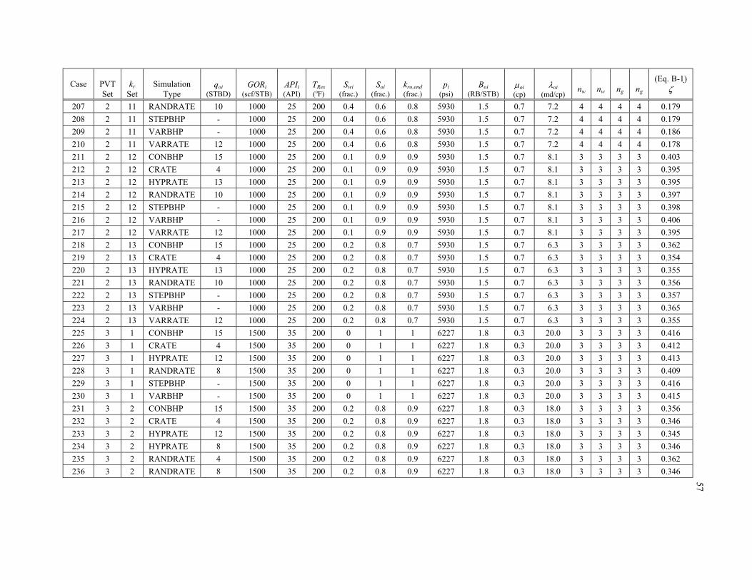
57
Case
PVT Set
kr
Set
Simulation
Type
qoi
(STBD)
GORi
(scf/STB)
APIi (API)
TRes (oF)
Swi
(frac.)
Soi
(frac.)
kro,end (frac.)
pi
(psi)
Boi
(RB/STB)
oi (cp)
oi
(md/cp)
nw
nw
ng
ng
(Eq. B-1)
207 2 11 RANDRATE 10 1000 25 200 0.4 0.6 0.8 5930 1.5 0.7 7.2 4 4 4 4 0.179
208 2 11 STEPBHP - 1000 25 200 0.4 0.6 0.8 5930 1.5 0.7 7.2 4 4 4 4 0.179
209 2 11 VARBHP - 1000 25 200 0.4 0.6 0.8 5930 1.5 0.7 7.2 4 4 4 4 0.186
210 2 11 VARRATE 12 1000 25 200 0.4 0.6 0.8 5930 1.5 0.7 7.2 4 4 4 4 0.178
211 2 12 CONBHP 15 1000 25 200 0.1 0.9 0.9 5930 1.5 0.7 8.1 3 3 3 3 0.403
212 2 12 CRATE 4 1000 25 200 0.1 0.9 0.9 5930 1.5 0.7 8.1 3 3 3 3 0.395
213 2 12 HYPRATE 13 1000 25 200 0.1 0.9 0.9 5930 1.5 0.7 8.1 3 3 3 3 0.395
214 2 12 RANDRATE 10 1000 25 200 0.1 0.9 0.9 5930 1.5 0.7 8.1 3 3 3 3 0.397
215 2 12 STEPBHP - 1000 25 200 0.1 0.9 0.9 5930 1.5 0.7 8.1 3 3 3 3 0.398
216 2 12 VARBHP - 1000 25 200 0.1 0.9 0.9 5930 1.5 0.7 8.1 3 3 3 3 0.406
217 2 12 VARRATE 12 1000 25 200 0.1 0.9 0.9 5930 1.5 0.7 8.1 3 3 3 3 0.395
218 2 13 CONBHP 15 1000 25 200 0.2 0.8 0.7 5930 1.5 0.7 6.3 3 3 3 3 0.362
219 2 13 CRATE 4 1000 25 200 0.2 0.8 0.7 5930 1.5 0.7 6.3 3 3 3 3 0.354
220 2 13 HYPRATE 13 1000 25 200 0.2 0.8 0.7 5930 1.5 0.7 6.3 3 3 3 3 0.355
221 2 13 RANDRATE 10 1000 25 200 0.2 0.8 0.7 5930 1.5 0.7 6.3 3 3 3 3 0.356
222 2 13 STEPBHP - 1000 25 200 0.2 0.8 0.7 5930 1.5 0.7 6.3 3 3 3 3 0.357
223 2 13 VARBHP - 1000 25 200 0.2 0.8 0.7 5930 1.5 0.7 6.3 3 3 3 3 0.365
224 2 13 VARRATE 12 1000 25 200 0.2 0.8 0.7 5930 1.5 0.7 6.3 3 3 3 3 0.355
225 3 1 CONBHP 15 1500 35 200 0 1 1 6227 1.8 0.3 20.0 3 3 3 3 0.416
226 3 1 CRATE 4 1500 35 200 0 1 1 6227 1.8 0.3 20.0 3 3 3 3 0.412
227 3 1 HYPRATE 12 1500 35 200 0 1 1 6227 1.8 0.3 20.0 3 3 3 3 0.413
228 3 1 RANDRATE 8 1500 35 200 0 1 1 6227 1.8 0.3 20.0 3 3 3 3 0.409
229 3 1 STEPBHP - 1500 35 200 0 1 1 6227 1.8 0.3 20.0 3 3 3 3 0.416
230 3 1 VARBHP - 1500 35 200 0 1 1 6227 1.8 0.3 20.0 3 3 3 3 0.415
231 3 2 CONBHP 15 1500 35 200 0.2 0.8 0.9 6227 1.8 0.3 18.0 3 3 3 3 0.356
232 3 2 CRATE 4 1500 35 200 0.2 0.8 0.9 6227 1.8 0.3 18.0 3 3 3 3 0.346
233 3 2 HYPRATE 12 1500 35 200 0.2 0.8 0.9 6227 1.8 0.3 18.0 3 3 3 3 0.345
234 3 2 HYPRATE 8 1500 35 200 0.2 0.8 0.9 6227 1.8 0.3 18.0 3 3 3 3 0.346
235 3 2 RANDRATE 4 1500 35 200 0.2 0.8 0.9 6227 1.8 0.3 18.0 3 3 3 3 0.362
236 3 2 RANDRATE 8 1500 35 200 0.2 0.8 0.9 6227 1.8 0.3 18.0 3 3 3 3 0.346

58
Case
PVT Set
kr
Set
Simulation
Type
qoi
(STBD)
GORi
(scf/STB)
APIi (API)
TRes (oF)
Swi
(frac.)
Soi
(frac.)
kro,end (frac.)
pi
(psi)
Boi
(RB/STB)
oi (cp)
oi
(md/cp)
nw
nw
ng
ng
(Eq. B-1)
237 3 2 STEPBHP - 1500 35 200 0.2 0.8 0.9 6227 1.8 0.3 18.0 3 3 3 3 0.354
238 3 2 VARBHP - 1500 35 200 0.2 0.8 0.9 6227 1.8 0.3 18.0 3 3 3 3 0.354
239 3 2 VARRATE 8 1500 35 200 0.2 0.8 0.9 6227 1.8 0.3 18.0 3 3 3 3 0.348
240 3 3 CONBHP 15 1500 35 200 0.4 0.6 0.8 6227 1.8 0.3 16.0 3 3 3 3 0.292
241 3 3 CRATE 2 1500 35 200 0.4 0.6 0.8 6227 1.8 0.3 16.0 3 3 3 3 0.282
242 3 3 CRATE 4 1500 35 200 0.4 0.6 0.8 6227 1.8 0.3 16.0 3 3 3 3 0.281
243 3 3 HYPRATE 12 1500 35 200 0.4 0.6 0.8 6227 1.8 0.3 16.0 3 3 3 3 0.282
244 3 3 HYPRATE 8 1500 35 200 0.4 0.6 0.8 6227 1.8 0.3 16.0 3 3 3 3 0.281
245 3 3 RANDRATE 4 1500 35 200 0.4 0.6 0.8 6227 1.8 0.3 16.0 3 3 3 3 0.282
246 3 3 RANDRATE 8 1500 35 200 0.4 0.6 0.8 6227 1.8 0.3 16.0 3 3 3 3 0.281
247 3 3 STEPBHP - 1500 35 200 0.4 0.6 0.8 6227 1.8 0.3 16.0 3 3 3 3 0.289
248 3 3 VARBHP - 1500 35 200 0.4 0.6 0.8 6227 1.8 0.3 16.0 3 3 3 3 0.289
249 3 3 VARRATE 8 1500 35 200 0.4 0.6 0.8 6227 1.8 0.3 16.0 3 3 3 3 0.281
250 3 4 CONBHP 15 1500 35 200 0 1 1 6227 1.8 0.3 20.0 3 3 4 3 0.285
251 3 4 CRATE 4 1500 35 200 0 1 1 6227 1.8 0.3 20.0 3 3 4 3 0.279
252 3 4 HYPRATE 12 1500 35 200 0 1 1 6227 1.8 0.3 20.0 3 3 4 3 0.277
253 3 4 HYPRATE 8 1500 35 200 0 1 1 6227 1.8 0.3 20.0 3 3 4 3 0.318
254 3 4 RANDRATE 8 1500 35 200 0 1 1 6227 1.8 0.3 20.0 3 3 4 3 0.278
255 3 4 STEPBHP - 1500 35 200 0 1 1 6227 1.8 0.3 20.0 3 3 4 3 0.286
256 3 4 VARBHP - 1500 35 200 0 1 1 6227 1.8 0.3 20.0 3 3 4 3 0.285
257 3 5 CONBHP 15 1500 35 200 0.4 0.6 0.8 6227 1.8 0.3 16.0 3 3 4 3 0.180
258 3 5 CRATE 2 1500 35 200 0.4 0.6 0.8 6227 1.8 0.3 16.0 3 3 4 3 0.174
259 3 5 CRATE 4 1500 35 200 0.4 0.6 0.8 6227 1.8 0.3 16.0 3 3 4 3 0.173
260 3 5 HYPRATE 12 1500 35 200 0.4 0.6 0.8 6227 1.8 0.3 16.0 3 3 4 3 0.174
261 3 5 HYPRATE 8 1500 35 200 0.4 0.6 0.8 6227 1.8 0.3 16.0 3 3 4 3 0.173
262 3 5 RANDRATE 4 1500 35 200 0.4 0.6 0.8 6227 1.8 0.3 16.0 3 3 4 3 0.173
263 3 5 RANDRATE 8 1500 35 200 0.4 0.6 0.8 6227 1.8 0.3 16.0 3 3 4 3 0.173
264 3 5 STEPBHP - 1500 35 200 0.4 0.6 0.8 6227 1.8 0.3 16.0 3 3 4 3 0.179
265 3 5 VARBHP - 1500 35 200 0.4 0.6 0.8 6227 1.8 0.3 16.0 3 3 4 3 0.179
266 3 5 VARRATE 4 1500 35 200 0.4 0.6 0.8 6227 1.8 0.3 16.0 3 3 4 3 0.174

59
Case
PVT Set
kr
Set
Simulation
Type
qoi
(STBD)
GORi
(scf/STB)
APIi (API)
TRes (oF)
Swi
(frac.)
Soi
(frac.)
kro,end (frac.)
pi
(psi)
Boi
(RB/STB)
oi (cp)
oi
(md/cp)
nw
nw
ng
ng
(Eq. B-1)
267 3 5 VARRATE 8 1500 35 200 0.4 0.6 0.8 6227 1.8 0.3 16.0 3 3 4 3 0.173
268 3 6 CONBHP 15 1500 35 200 0 1 1 6227 1.8 0.3 20.0 2 2 2 2 0.649
269 3 6 CRATE 4 1500 35 200 0 1 1 6227 1.8 0.3 20.0 2 2 2 2 0.636
270 3 6 RANDRATE 8 1500 35 200 0 1 1 6227 1.8 0.3 20.0 2 2 2 2 0.636
271 3 6 STEPBHP - 1500 35 200 0 1 1 6227 1.8 0.3 20.0 2 2 2 2 0.638
272 3 6 VARBHP - 1500 35 200 0 1 1 6227 1.8 0.3 20.0 2 2 2 2 0.641
273 3 6 VARRATE 12 1500 35 200 0 1 1 6227 1.8 0.3 20.0 2 2 2 2 0.636
274 3 7 CONBHP 15 1500 35 200 0.2 0.8 0.9 6227 1.8 0.3 18.0 2 2 2 2 0.725
275 3 7 CRATE 4 1500 35 200 0.2 0.8 0.9 6227 1.8 0.3 18.0 2 2 2 2 0.716
276 3 7 STEPBHP - 1500 35 200 0.2 0.8 0.9 6227 1.8 0.3 18.0 2 2 2 2 0.718
277 3 7 VARBHP - 1500 35 200 0.2 0.8 0.9 6227 1.8 0.3 18.0 2 2 2 2 0.720
278 3 7 VARRATE 12 1500 35 200 0.2 0.8 0.9 6227 1.8 0.3 18.0 2 2 2 2 0.716
279 3 8 CONBHP 15 1500 35 200 0.4 0.6 0.8 6227 1.8 0.3 16.0 2 2 2 2 0.527
280 3 8 CRATE 4 1500 35 200 0.4 0.6 0.8 6227 1.8 0.3 16.0 2 2 2 2 0.516
281 3 8 HYPRATE 13 1500 35 200 0.4 0.6 0.8 6227 1.8 0.3 16.0 2 2 2 2 0.517
282 3 8 RANDRATE 10 1500 35 200 0.4 0.6 0.8 6227 1.8 0.3 16.0 2 2 2 2 0.516
283 3 8 STEPBHP - 1500 35 200 0.4 0.6 0.8 6227 1.8 0.3 16.0 2 2 2 2 0.519
284 3 8 VARBHP - 1500 35 200 0.4 0.6 0.8 6227 1.8 0.3 16.0 2 2 2 2 0.521
285 3 8 VARRATE 12 1500 35 200 0.4 0.6 0.8 6227 1.8 0.3 16.0 2 2 2 2 0.517
286 3 9 CONBHP 15 1500 35 200 0 1 1 6227 1.8 0.3 20.0 4 4 4 4 0.249
287 3 9 CRATE 4 1500 35 200 0 1 1 6227 1.8 0.3 20.0 4 4 4 4 0.243
288 3 9 HYPRATE 17 1500 35 200 0 1 1 6227 1.8 0.3 20.0 4 4 4 4 0.241
289 3 9 RANDRATE 8 1500 35 200 0 1 1 6227 1.8 0.3 20.0 4 4 4 4 0.248
290 3 9 STEPBHP - 1500 35 200 0 1 1 6227 1.8 0.3 20.0 4 4 4 4 0.244
291 3 9 VARBHP - 1500 35 200 0 1 1 6227 1.8 0.3 20.0 4 4 4 4 0.255
292 3 9 VARRATE 12 1500 35 200 0 1 1 6227 1.8 0.3 20.0 4 4 4 4 0.246
293 3 10 CONBHP 15 1500 35 200 0.2 0.8 0.9 6227 1.8 0.3 18.0 4 4 4 4 0.200
294 3 10 CRATE 4 1500 35 200 0.2 0.8 0.9 6227 1.8 0.3 18.0 4 4 4 4 0.196
295 3 10 HYPRATE 17 1500 35 200 0.2 0.8 0.9 6227 1.8 0.3 18.0 4 4 4 4 0.196
296 3 10 RANDRATE 10 1500 35 200 0.2 0.8 0.9 6227 1.8 0.3 18.0 4 4 4 4 0.197

60
Case
PVT Set
kr
Set
Simulation
Type
qoi
(STBD)
GORi
(scf/STB)
APIi (API)
TRes (oF)
Swi
(frac.)
Soi
(frac.)
kro,end (frac.)
pi
(psi)
Boi
(RB/STB)
oi (cp)
oi
(md/cp)
nw
nw
ng
ng
(Eq. B-1)
297 3 10 STEPBHP - 1500 35 200 0.2 0.8 0.9 6227 1.8 0.3 18.0 4 4 4 4 0.197
298 3 10 VARBHP - 1500 35 200 0.2 0.8 0.9 6227 1.8 0.3 18.0 4 4 4 4 0.202
299 3 10 VARRATE 12 1500 35 200 0.2 0.8 0.9 6227 1.8 0.3 18.0 4 4 4 4 0.196
300 3 11 CONBHP 15 1500 35 200 0.4 0.6 0.8 6227 1.8 0.3 16.0 4 4 4 4 0.155
301 3 11 CRATE 4 1500 35 200 0.4 0.6 0.8 6227 1.8 0.3 16.0 4 4 4 4 0.151
302 3 11 HYPRATE 17 1500 35 200 0.4 0.6 0.8 6227 1.8 0.3 16.0 4 4 4 4 0.152
303 3 11 RANDRATE 10 1500 35 200 0.4 0.6 0.8 6227 1.8 0.3 16.0 4 4 4 4 0.152
304 3 11 STEPBHP - 1500 35 200 0.4 0.6 0.8 6227 1.8 0.3 16.0 4 4 4 4 0.152
305 3 11 VARBHP - 1500 35 200 0.4 0.6 0.8 6227 1.8 0.3 16.0 4 4 4 4 0.157
306 3 11 VARRATE 12 1500 35 200 0.4 0.6 0.8 6227 1.8 0.3 16.0 4 4 4 4 0.152
307 3 12 CONBHP 15 1500 35 200 0.1 0.9 0.9 6227 1.8 0.3 18.0 3 3 3 3 0.415
308 3 12 CRATE 4 1500 35 200 0.1 0.9 0.9 6227 1.8 0.3 18.0 3 3 3 3 0.405
309 3 12 HYPRATE 13 1500 35 200 0.1 0.9 0.9 6227 1.8 0.3 18.0 3 3 3 3 0.405
310 3 12 RANDRATE 10 1500 35 200 0.1 0.9 0.9 6227 1.8 0.3 18.0 3 3 3 3 0.407
311 3 12 STEPBHP - 1500 35 200 0.1 0.9 0.9 6227 1.8 0.3 18.0 3 3 3 3 0.408
312 3 12 VARBHP - 1500 35 200 0.1 0.9 0.9 6227 1.8 0.3 18.0 3 3 3 3 0.415
313 3 12 VARRATE 12 1500 35 200 0.1 0.9 0.9 6227 1.8 0.3 18.0 3 3 3 3 0.405
314 3 13 CONBHP 15 1500 35 200 0.2 0.8 0.7 6227 1.8 0.3 14.0 3 3 3 3 0.356
315 3 13 CRATE 4 1500 35 200 0.2 0.8 0.7 6227 1.8 0.3 14.0 3 3 3 3 0.345
316 3 13 HYPRATE 13 1500 35 200 0.2 0.8 0.7 6227 1.8 0.3 14.0 3 3 3 3 0.345
317 3 13 RANDRATE 10 1500 35 200 0.2 0.8 0.7 6227 1.8 0.3 14.0 3 3 3 3 0.346
318 3 13 STEPBHP - 1500 35 200 0.2 0.8 0.7 6227 1.8 0.3 14.0 3 3 3 3 0.349
319 3 13 VARBHP - 1500 35 200 0.2 0.8 0.7 6227 1.8 0.3 14.0 3 3 3 3 0.356
320 3 13 VARRATE 12 1500 35 200 0.2 0.8 0.7 6227 1.8 0.3 14.0 3 3 3 3 0.346
321 4 1 CONBHP 15 500 15 250 0 1 1 4935 1.3 2.3 3.3 3 3 3 3 0.497
322 4 1 CRATE 4 500 15 250 0 1 1 4935 1.3 2.3 3.3 3 3 3 3 0.508
323 4 1 HYPRATE 12 500 15 250 0 1 1 4935 1.3 2.3 3.3 3 3 3 3 0.525
324 4 1 HYPRATE 16 500 15 250 0 1 1 4935 1.3 2.3 3.3 3 3 3 3 0.494
325 4 1 RANDRATE 8 500 15 250 0 1 1 4935 1.3 2.3 3.3 3 3 3 3 0.502
326 4 1 STEPBHP - 500 15 250 0 1 1 4935 1.3 2.3 3.3 3 3 3 3 0.500

61
Case
PVT Set
kr
Set
Simulation
Type
qoi
(STBD)
GORi
(scf/STB)
APIi (API)
TRes (oF)
Swi
(frac.)
Soi
(frac.)
kro,end (frac.)
pi
(psi)
Boi
(RB/STB)
oi (cp)
oi
(md/cp)
nw
nw
ng
ng
(Eq. B-1)
327 4 1 VARBHP - 500 15 250 0 1 1 4935 1.3 2.3 3.3 3 3 3 3 0.500
328 4 2 CONBHP 15 500 15 250 0.2 0.8 0.9 4935 1.3 2.3 3.0 3 3 3 3 0.466
329 4 2 CRATE 4 500 15 250 0.2 0.8 0.9 4935 1.3 2.3 3.0 3 3 3 3 0.461
330 4 2 HYPRATE 12 500 15 250 0.2 0.8 0.9 4935 1.3 2.3 3.0 3 3 3 3 0.460
331 4 2 HYPRATE 16 500 15 250 0.2 0.8 0.9 4935 1.3 2.3 3.0 3 3 3 3 0.460
332 4 2 HYPRATE 8 500 15 250 0.2 0.8 0.9 4935 1.3 2.3 3.0 3 3 3 3 0.463
333 4 2 RANDRATE 8 500 15 250 0.2 0.8 0.9 4935 1.3 2.3 3.0 3 3 3 3 0.461
334 4 2 STEPBHP - 500 15 250 0.2 0.8 0.9 4935 1.3 2.3 3.0 3 3 3 3 0.467
335 4 2 VARBHP - 500 15 250 0.2 0.8 0.9 4935 1.3 2.3 3.0 3 3 3 3 0.468
336 4 3 CONBHP 15 500 15 250 0.4 0.6 0.8 4935 1.3 2.3 2.6 3 3 3 3 0.430
337 4 3 CRATE 2 500 15 250 0.4 0.6 0.8 4935 1.3 2.3 2.6 3 3 3 3 0.427
338 4 3 CRATE 4 500 15 250 0.4 0.6 0.8 4935 1.3 2.3 2.6 3 3 3 3 0.422
339 4 3 HYPRATE 12 500 15 250 0.4 0.6 0.8 4935 1.3 2.3 2.6 3 3 3 3 0.423
340 4 3 HYPRATE 16 500 15 250 0.4 0.6 0.8 4935 1.3 2.3 2.6 3 3 3 3 0.424
341 4 3 HYPRATE 8 500 15 250 0.4 0.6 0.8 4935 1.3 2.3 2.6 3 3 3 3 0.422
342 4 3 RANDRATE 4 500 15 250 0.4 0.6 0.8 4935 1.3 2.3 2.6 3 3 3 3 0.425
343 4 3 RANDRATE 8 500 15 250 0.4 0.6 0.8 4935 1.3 2.3 2.6 3 3 3 3 0.422
344 4 3 STEPBHP - 500 15 250 0.4 0.6 0.8 4935 1.3 2.3 2.6 3 3 3 3 0.429
345 4 3 VARBHP - 500 15 250 0.4 0.6 0.8 4935 1.3 2.3 2.6 3 3 3 3 0.430
346 4 3 VARRATE 8 500 15 250 0.4 0.6 0.8 4935 1.3 2.3 2.6 3 3 3 3 0.422
347 4 4 CONBHP 15 500 15 250 0 1 1 4935 1.3 2.3 3.3 3 3 4 3 0.416
348 4 4 CRATE 4 500 15 250 0 1 1 4935 1.3 2.3 3.3 3 3 4 3 0.423
349 4 4 HYPRATE 12 500 15 250 0 1 1 4935 1.3 2.3 3.3 3 3 4 3 0.419
350 4 4 HYPRATE 16 500 15 250 0 1 1 4935 1.3 2.3 3.3 3 3 4 3 0.412
351 4 4 RANDRATE 8 500 15 250 0 1 1 4935 1.3 2.3 3.3 3 3 4 3 0.419
352 4 4 STEPBHP - 500 15 250 0 1 1 4935 1.3 2.3 3.3 3 3 4 3 0.419
353 4 4 VARBHP - 500 15 250 0 1 1 4935 1.3 2.3 3.3 3 3 4 3 0.420
354 4 5 CRATE 2 500 15 250 0.4 0.6 0.8 4935 1.3 2.3 2.6 3 3 4 3 0.334
355 4 5 CRATE 4 500 15 250 0.4 0.6 0.8 4935 1.3 2.3 2.6 3 3 4 3 0.330
356 4 5 HYPRATE 12 500 15 250 0.4 0.6 0.8 4935 1.3 2.3 2.6 3 3 4 3 0.331

62
Case
PVT Set
kr
Set
Simulation
Type
qoi
(STBD)
GORi
(scf/STB)
APIi (API)
TRes (oF)
Swi
(frac.)
Soi
(frac.)
kro,end (frac.)
pi
(psi)
Boi
(RB/STB)
oi (cp)
oi
(md/cp)
nw
nw
ng
ng
(Eq. B-1)
357 4 5 HYPRATE 16 500 15 250 0.4 0.6 0.8 4935 1.3 2.3 2.6 3 3 4 3 0.332
358 4 5 HYPRATE 8 500 15 250 0.4 0.6 0.8 4935 1.3 2.3 2.6 3 3 4 3 0.330
359 4 5 RANDRATE 4 500 15 250 0.4 0.6 0.8 4935 1.3 2.3 2.6 3 3 4 3 0.333
360 4 5 RANDRATE 8 500 15 250 0.4 0.6 0.8 4935 1.3 2.3 2.6 3 3 4 3 0.330
361 4 5 STEPBHP - 500 15 250 0.4 0.6 0.8 4935 1.3 2.3 2.6 3 3 4 3 0.338
362 4 5 VARBHP - 500 15 250 0.4 0.6 0.8 4935 1.3 2.3 2.6 3 3 4 3 0.339
363 4 5 VARRATE 8 500 15 250 0.4 0.6 0.8 4935 1.3 2.3 2.6 3 3 4 3 0.330
364 4 6 CONBHP 15 500 15 250 0 1 1 4935 1.3 2.3 3.3 2 2 2 2 0.628
365 4 6 CRATE 4 500 15 250 0 1 1 4935 1.3 2.3 3.3 2 2 2 2 0.622
366 4 6 RANDRATE 8 500 15 250 0 1 1 4935 1.3 2.3 3.3 2 2 2 2 0.623
367 4 6 STEPBHP - 500 15 250 0 1 1 4935 1.3 2.3 3.3 2 2 2 2 0.624
368 4 6 VARBHP - 500 15 250 0 1 1 4935 1.3 2.3 3.3 2 2 2 2 0.628
369 4 6 VARRATE 12 500 15 250 0 1 1 4935 1.3 2.3 3.3 2 2 2 2 0.623
370 4 7 CONBHP 15 500 15 250 0.2 0.8 0.9 4935 1.3 2.3 3.0 2 2 2 2 0.663
371 4 7 CRATE 4 500 15 250 0.2 0.8 0.9 4935 1.3 2.3 3.0 2 2 2 2 0.658
372 4 7 STEPBHP - 500 15 250 0.2 0.8 0.9 4935 1.3 2.3 3.0 2 2 2 2 0.659
373 4 7 VARBHP - 500 15 250 0.2 0.8 0.9 4935 1.3 2.3 3.0 2 2 2 2 0.663
374 4 7 VARRATE 12 500 15 250 0.2 0.8 0.9 4935 1.3 2.3 3.0 2 2 2 2 0.659
375 4 8 CONBHP 15 500 15 250 0.4 0.6 0.8 4935 1.3 2.3 2.6 2 2 2 2 0.587
376 4 8 CRATE 4 500 15 250 0.4 0.6 0.8 4935 1.3 2.3 2.6 2 2 2 2 0.580
377 4 8 HYPRATE 13 500 15 250 0.4 0.6 0.8 4935 1.3 2.3 2.6 2 2 2 2 0.582
378 4 8 RANDRATE 10 500 15 250 0.4 0.6 0.8 4935 1.3 2.3 2.6 2 2 2 2 0.581
379 4 8 STEPBHP - 500 15 250 0.4 0.6 0.8 4935 1.3 2.3 2.6 2 2 2 2 0.581
380 4 8 VARRATE 12 500 15 250 0.4 0.6 0.8 4935 1.3 2.3 2.6 2 2 2 2 0.582
381 4 9 CONBHP 15 500 15 250 0 1 1 4935 1.3 2.3 3.3 4 4 4 4 0.381
382 4 9 CRATE 4 500 15 250 0 1 1 4935 1.3 2.3 3.3 4 4 4 4 0.397
383 4 9 HYPRATE 17 500 15 250 0 1 1 4935 1.3 2.3 3.3 4 4 4 4 0.378
384 4 9 STEPBHP 500 15 250 0 1 1 4935 1.3 2.3 3.3 4 4 4 4 0.381
385 4 10 CONBHP 15 500 15 250 0.2 0.8 0.9 4935 1.3 2.3 3.0 4 4 4 4 0.334
386 4 10 CRATE 4 500 15 250 0.2 0.8 0.9 4935 1.3 2.3 3.0 4 4 4 4 0.332

63
Case
PVT Set
kr
Set
Simulation
Type
qoi
(STBD)
GORi
(scf/STB)
APIi (API)
TRes (oF)
Swi
(frac.)
Soi
(frac.)
kro,end (frac.)
pi
(psi)
Boi
(RB/STB)
oi (cp)
oi
(md/cp)
nw
nw
ng
ng
(Eq. B-1)
387 4 10 HYPRATE 17 500 15 250 0.2 0.8 0.9 4935 1.3 2.3 3.0 4 4 4 4 0.330
388 4 10 STEPBHP - 500 15 250 0.2 0.8 0.9 4935 1.3 2.3 3.0 4 4 4 4 0.332
389 4 10 VARBHP - 500 15 250 0.2 0.8 0.9 4935 1.3 2.3 3.0 4 4 4 4 0.346
390 4 10 VARRATE 12 500 15 250 0.2 0.8 0.9 4935 1.3 2.3 3.0 4 4 4 4 0.331
391 4 11 CONBHP 15 500 15 250 0.4 0.6 0.8 4935 1.3 2.3 2.6 4 4 4 4 0.292
392 4 11 CRATE 4 500 15 250 0.4 0.6 0.8 4935 1.3 2.3 2.6 4 4 4 4 0.287
393 4 11 HYPRATE 17 500 15 250 0.4 0.6 0.8 4935 1.3 2.3 2.6 4 4 4 4 0.290
394 4 11 RANDRATE 10 500 15 250 0.4 0.6 0.8 4935 1.3 2.3 2.6 4 4 4 4 0.291
395 4 11 STEPBHP - 500 15 250 0.4 0.6 0.8 4935 1.3 2.3 2.6 4 4 4 4 0.289
396 4 11 VARBHP - 500 15 250 0.4 0.6 0.8 4935 1.3 2.3 2.6 4 4 4 4 0.297
397 4 11 VARRATE 12 500 15 250 0.4 0.6 0.8 4935 1.3 2.3 2.6 4 4 4 4 0.288
398 4 12 CONBHP 15 500 15 250 0.1 0.9 0.9 4935 1.3 2.3 3.0 3 3 3 3 0.496
399 4 12 CRATE 4 500 15 250 0.1 0.9 0.9 4935 1.3 2.3 3.0 3 3 3 3 0.490
400 4 12 HYPRATE 13 500 15 250 0.1 0.9 0.9 4935 1.3 2.3 3.0 3 3 3 3 0.490
401 4 12 RANDRATE 10 500 15 250 0.1 0.9 0.9 4935 1.3 2.3 3.0 3 3 3 3 0.494
402 4 12 STEPBHP - 500 15 250 0.1 0.9 0.9 4935 1.3 2.3 3.0 3 3 3 3 0.491
403 4 12 VARBHP - 500 15 250 0.1 0.9 0.9 4935 1.3 2.3 3.0 3 3 3 3 0.500
404 4 12 VARRATE 12 500 15 250 0.1 0.9 0.9 4935 1.3 2.3 3.0 3 3 3 3 0.490
405 4 13 CONBHP 15 500 15 250 0.2 0.8 0.7 4935 1.3 2.3 2.3 3 3 3 3 0.465
406 4 13 CRATE 4 500 15 250 0.2 0.8 0.7 4935 1.3 2.3 2.3 3 3 3 3 0.459
407 4 13 HYPRATE 13 500 15 250 0.2 0.8 0.7 4935 1.3 2.3 2.3 3 3 3 3 0.460
408 4 13 RANDRATE 10 500 15 250 0.2 0.8 0.7 4935 1.3 2.3 2.3 3 3 3 3 0.462
409 4 13 STEPBHP - 500 15 250 0.2 0.8 0.7 4935 1.3 2.3 2.3 3 3 3 3 0.461
410 4 13 VARBHP - 500 15 250 0.2 0.8 0.7 4935 1.3 2.3 2.3 3 3 3 3 0.470
411 4 13 VARRATE 12 500 15 250 0.2 0.8 0.7 4935 1.3 2.3 2.3 3 3 3 3 0.459
412 5 1 CONBHP 15 1000 25 250 0 1 1 6587 1.5 0.5 13.0 3 3 3 3 0.419
413 5 1 CRATE 4 1000 25 250 0 1 1 6587 1.5 0.5 13.0 3 3 3 3 0.426
414 5 1 HYPRATE 16 1000 25 250 0 1 1 6587 1.5 0.5 13.0 3 3 3 3 0.417
415 5 1 RANDRATE 8 1000 25 250 0 1 1 6587 1.5 0.5 13.0 3 3 3 3 0.419
416 5 1 STEPBHP - 1000 25 250 0 1 1 6587 1.5 0.5 13.0 3 3 3 3 0.419

64
Case
PVT Set
kr
Set
Simulation
Type
qoi
(STBD)
GORi
(scf/STB)
APIi (API)
TRes (oF)
Swi
(frac.)
Soi
(frac.)
kro,end (frac.)
pi
(psi)
Boi
(RB/STB)
oi (cp)
oi
(md/cp)
nw
nw
ng
ng
(Eq. B-1)
417 5 1 VARBHP - 1000 25 250 0 1 1 6587 1.5 0.5 13.0 3 3 3 3 0.419
418 5 2 CONBHP 15 1000 25 250 0.2 0.8 0.9 6587 1.5 0.5 11.7 3 3 3 3 0.374
419 5 2 CRATE 4 1000 25 250 0.2 0.8 0.9 6587 1.5 0.5 11.7 3 3 3 3 0.366
420 5 2 HYPRATE 12 1000 25 250 0.2 0.8 0.9 6587 1.5 0.5 11.7 3 3 3 3 0.365
421 5 2 HYPRATE 16 1000 25 250 0.2 0.8 0.9 6587 1.5 0.5 11.7 3 3 3 3 0.365
422 5 2 HYPRATE 8 1000 25 250 0.2 0.8 0.9 6587 1.5 0.5 11.7 3 3 3 3 0.368
423 5 2 RANDRATE 8 1000 25 250 0.2 0.8 0.9 6587 1.5 0.5 11.7 3 3 3 3 0.366
424 5 2 STEPBHP - 1000 25 250 0.2 0.8 0.9 6587 1.5 0.5 11.7 3 3 3 3 0.372
425 5 2 VARBHP - 1000 25 250 0.2 0.8 0.9 6587 1.5 0.5 11.7 3 3 3 3 0.372
426 5 3 CONBHP 15 1000 25 250 0.4 0.6 0.8 6587 1.5 0.5 10.4 3 3 3 3 0.324
427 5 3 CRATE 2 1000 25 250 0.4 0.6 0.8 6587 1.5 0.5 10.4 3 3 3 3 0.317
428 5 3 CRATE 4 1000 25 250 0.4 0.6 0.8 6587 1.5 0.5 10.4 3 3 3 3 0.315
429 5 3 HYPRATE 12 1000 25 250 0.4 0.6 0.8 6587 1.5 0.5 10.4 3 3 3 3 0.315
430 5 3 HYPRATE 16 1000 25 250 0.4 0.6 0.8 6587 1.5 0.5 10.4 3 3 3 3 0.315
431 5 3 HYPRATE 8 1000 25 250 0.4 0.6 0.8 6587 1.5 0.5 10.4 3 3 3 3 0.315
432 5 3 RANDRATE 4 1000 25 250 0.4 0.6 0.8 6587 1.5 0.5 10.4 3 3 3 3 0.316
433 5 3 RANDRATE 8 1000 25 250 0.4 0.6 0.8 6587 1.5 0.5 10.4 3 3 3 3 0.315
434 5 3 STEPBHP - 1000 25 250 0.4 0.6 0.8 6587 1.5 0.5 10.4 3 3 3 3 0.321
435 5 3 VARBHP - 1000 25 250 0.4 0.6 0.8 6587 1.5 0.5 10.4 3 3 3 3 0.322
436 5 3 VARRATE 8 1000 25 250 0.4 0.6 0.8 6587 1.5 0.5 10.4 3 3 3 3 0.315
437 5 4 CONBHP 15 1000 25 250 0 1 1 6587 1.5 0.5 13.0 3 3 4 3 0.314
438 5 4 CRATE 4 1000 25 250 0 1 1 6587 1.5 0.5 13.0 3 3 4 3 0.313
439 5 4 HYPRATE 12 1000 25 250 0 1 1 6587 1.5 0.5 13.0 3 3 4 3 0.320
440 5 4 HYPRATE 16 1000 25 250 0 1 1 6587 1.5 0.5 13.0 3 3 4 3 0.306
441 5 4 RANDRATE 8 1000 25 250 0 1 1 6587 1.5 0.5 13.0 3 3 4 3 0.310
442 5 4 STEPBHP - 1000 25 250 0 1 1 6587 1.5 0.5 13.0 3 3 4 3 0.315
443 5 4 VARBHP - 1000 25 250 0 1 1 6587 1.5 0.5 13.0 3 3 4 3 0.315
444 5 5 CONBHP 15 1000 25 250 0.4 0.6 0.8 6587 1.5 0.5 10.4 3 3 4 3 0.218
445 5 5 CRATE 2 1000 25 250 0.4 0.6 0.8 6587 1.5 0.5 10.4 3 3 4 3 0.214
446 5 5 CRATE 4 1000 25 250 0.4 0.6 0.8 6587 1.5 0.5 10.4 3 3 4 3 0.212

65
Case
PVT Set
kr
Set
Simulation
Type
qoi
(STBD)
GORi
(scf/STB)
APIi (API)
TRes (oF)
Swi
(frac.)
Soi
(frac.)
kro,end (frac.)
pi
(psi)
Boi
(RB/STB)
oi (cp)
oi
(md/cp)
nw
nw
ng
ng
(Eq. B-1)
447 5 5 HYPRATE 12 1000 25 250 0.4 0.6 0.8 6587 1.5 0.5 10.4 3 3 4 3 0.212
448 5 5 HYPRATE 16 1000 25 250 0.4 0.6 0.8 6587 1.5 0.5 10.4 3 3 4 3 0.212
449 5 5 HYPRATE 8 1000 25 250 0.4 0.6 0.8 6587 1.5 0.5 10.4 3 3 4 3 0.212
450 5 5 RANDRATE 4 1000 25 250 0.4 0.6 0.8 6587 1.5 0.5 10.4 3 3 4 3 0.213
451 5 5 RANDRATE 8 1000 25 250 0.4 0.6 0.8 6587 1.5 0.5 10.4 3 3 4 3 0.212
452 5 5 STEPBHP - 1000 25 250 0.4 0.6 0.8 6587 1.5 0.5 10.4 3 3 4 3 0.219
453 5 5 VARBHP - 1000 25 250 0.4 0.6 0.8 6587 1.5 0.5 10.4 3 3 4 3 0.218
454 5 5 VARRATE 8 1000 25 250 0.4 0.6 0.8 6587 1.5 0.5 10.4 3 3 4 3 0.212
455 5 6 CONBHP 15 1000 25 250 0 1 1 6587 1.5 0.5 13.0 2 2 2 2 0.594
456 5 6 CRATE 4 1000 25 250 0 1 1 6587 1.5 0.5 13.0 2 2 2 2 0.585
457 5 6 RANDRATE 8 1000 25 250 0 1 1 6587 1.5 0.5 13.0 2 2 2 2 0.585
458 5 6 STEPBHP - 1000 25 250 0 1 1 6587 1.5 0.5 13.0 2 2 2 2 0.587
459 5 6 VARBHP - 1000 25 250 0 1 1 6587 1.5 0.5 13.0 2 2 2 2 0.589
460 5 6 VARRATE 12 1000 25 250 0 1 1 6587 1.5 0.5 13.0 2 2 2 2 0.586
461 5 7 CONBHP 15 1000 25 250 0.2 0.8 0.9 6587 1.5 0.5 11.7 2 2 2 2 0.641
462 5 7 CRATE 4 1000 25 250 0.2 0.8 0.9 6587 1.5 0.5 11.7 2 2 2 2 0.635
463 5 7 STEPBHP - 1000 25 250 0.2 0.8 0.9 6587 1.5 0.5 11.7 2 2 2 2 0.636
464 5 7 VARBHP - 1000 25 250 0.2 0.8 0.9 6587 1.5 0.5 11.7 2 2 2 2 0.638
465 5 7 VARRATE 12 1000 25 250 0.2 0.8 0.9 6587 1.5 0.5 11.7 2 2 2 2 0.635
466 5 8 CONBHP 15 1000 25 250 0.4 0.6 0.8 6587 1.5 0.5 10.4 2 2 2 2 0.516
467 5 8 CRATE 4 1000 25 250 0.4 0.6 0.8 6587 1.5 0.5 10.4 2 2 2 2 0.507
468 5 8 HYPRATE 13 1000 25 250 0.4 0.6 0.8 6587 1.5 0.5 10.4 2 2 2 2 0.507
469 5 8 RANDRATE 10 1000 25 250 0.4 0.6 0.8 6587 1.5 0.5 10.4 2 2 2 2 0.507
470 5 8 STEPBHP - 1000 25 250 0.4 0.6 0.8 6587 1.5 0.5 10.4 2 2 2 2 0.509
471 5 8 VARRATE 12 1000 25 250 0.4 0.6 0.8 6587 1.5 0.5 10.4 2 2 2 2 0.507
472 5 9 CONBHP 15 1000 25 250 0 1 1 6587 1.5 0.5 13.0 4 4 4 4 0.282
473 5 9 CRATE 4 1000 25 250 0 1 1 6587 1.5 0.5 13.0 4 4 4 4 0.280
474 5 9 HYPRATE 17 1000 25 250 0 1 1 6587 1.5 0.5 13.0 4 4 4 4 0.275
475 5 9 RANDRATE 8 1000 25 250 0 1 1 6587 1.5 0.5 13.0 4 4 4 4 0.290
476 5 9 STEPBHP - 1000 25 250 0 1 1 6587 1.5 0.5 13.0 4 4 4 4 0.278
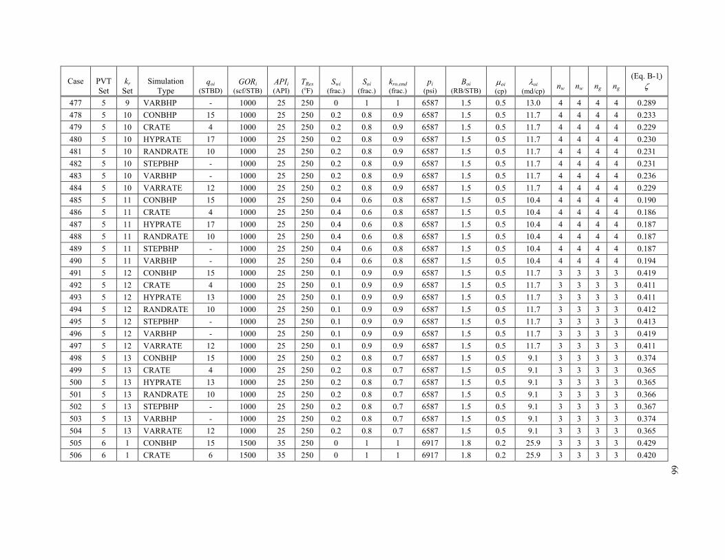
66
Case
PVT Set
kr
Set
Simulation
Type
qoi
(STBD)
GORi
(scf/STB)
APIi (API)
TRes (oF)
Swi
(frac.)
Soi
(frac.)
kro,end (frac.)
pi
(psi)
Boi
(RB/STB)
oi (cp)
oi
(md/cp)
nw
nw
ng
ng
(Eq. B-1)
477 5 9 VARBHP - 1000 25 250 0 1 1 6587 1.5 0.5 13.0 4 4 4 4 0.289
478 5 10 CONBHP 15 1000 25 250 0.2 0.8 0.9 6587 1.5 0.5 11.7 4 4 4 4 0.233
479 5 10 CRATE 4 1000 25 250 0.2 0.8 0.9 6587 1.5 0.5 11.7 4 4 4 4 0.229
480 5 10 HYPRATE 17 1000 25 250 0.2 0.8 0.9 6587 1.5 0.5 11.7 4 4 4 4 0.230
481 5 10 RANDRATE 10 1000 25 250 0.2 0.8 0.9 6587 1.5 0.5 11.7 4 4 4 4 0.231
482 5 10 STEPBHP - 1000 25 250 0.2 0.8 0.9 6587 1.5 0.5 11.7 4 4 4 4 0.231
483 5 10 VARBHP - 1000 25 250 0.2 0.8 0.9 6587 1.5 0.5 11.7 4 4 4 4 0.236
484 5 10 VARRATE 12 1000 25 250 0.2 0.8 0.9 6587 1.5 0.5 11.7 4 4 4 4 0.229
485 5 11 CONBHP 15 1000 25 250 0.4 0.6 0.8 6587 1.5 0.5 10.4 4 4 4 4 0.190
486 5 11 CRATE 4 1000 25 250 0.4 0.6 0.8 6587 1.5 0.5 10.4 4 4 4 4 0.186
487 5 11 HYPRATE 17 1000 25 250 0.4 0.6 0.8 6587 1.5 0.5 10.4 4 4 4 4 0.187
488 5 11 RANDRATE 10 1000 25 250 0.4 0.6 0.8 6587 1.5 0.5 10.4 4 4 4 4 0.187
489 5 11 STEPBHP - 1000 25 250 0.4 0.6 0.8 6587 1.5 0.5 10.4 4 4 4 4 0.187
490 5 11 VARBHP - 1000 25 250 0.4 0.6 0.8 6587 1.5 0.5 10.4 4 4 4 4 0.194
491 5 12 CONBHP 15 1000 25 250 0.1 0.9 0.9 6587 1.5 0.5 11.7 3 3 3 3 0.419
492 5 12 CRATE 4 1000 25 250 0.1 0.9 0.9 6587 1.5 0.5 11.7 3 3 3 3 0.411
493 5 12 HYPRATE 13 1000 25 250 0.1 0.9 0.9 6587 1.5 0.5 11.7 3 3 3 3 0.411
494 5 12 RANDRATE 10 1000 25 250 0.1 0.9 0.9 6587 1.5 0.5 11.7 3 3 3 3 0.412
495 5 12 STEPBHP - 1000 25 250 0.1 0.9 0.9 6587 1.5 0.5 11.7 3 3 3 3 0.413
496 5 12 VARBHP - 1000 25 250 0.1 0.9 0.9 6587 1.5 0.5 11.7 3 3 3 3 0.419
497 5 12 VARRATE 12 1000 25 250 0.1 0.9 0.9 6587 1.5 0.5 11.7 3 3 3 3 0.411
498 5 13 CONBHP 15 1000 25 250 0.2 0.8 0.7 6587 1.5 0.5 9.1 3 3 3 3 0.374
499 5 13 CRATE 4 1000 25 250 0.2 0.8 0.7 6587 1.5 0.5 9.1 3 3 3 3 0.365
500 5 13 HYPRATE 13 1000 25 250 0.2 0.8 0.7 6587 1.5 0.5 9.1 3 3 3 3 0.365
501 5 13 RANDRATE 10 1000 25 250 0.2 0.8 0.7 6587 1.5 0.5 9.1 3 3 3 3 0.366
502 5 13 STEPBHP - 1000 25 250 0.2 0.8 0.7 6587 1.5 0.5 9.1 3 3 3 3 0.367
503 5 13 VARBHP - 1000 25 250 0.2 0.8 0.7 6587 1.5 0.5 9.1 3 3 3 3 0.374
504 5 13 VARRATE 12 1000 25 250 0.2 0.8 0.7 6587 1.5 0.5 9.1 3 3 3 3 0.365
505 6 1 CONBHP 15 1500 35 250 0 1 1 6917 1.8 0.2 25.9 3 3 3 3 0.429
506 6 1 CRATE 6 1500 35 250 0 1 1 6917 1.8 0.2 25.9 3 3 3 3 0.420

67
Case
PVT Set
kr
Set
Simulation
Type
qoi
(STBD)
GORi
(scf/STB)
APIi (API)
TRes (oF)
Swi
(frac.)
Soi
(frac.)
kro,end (frac.)
pi
(psi)
Boi
(RB/STB)
oi (cp)
oi
(md/cp)
nw
nw
ng
ng
(Eq. B-1)
507 6 1 HYPRATE 10 1500 35 250 0 1 1 6917 1.8 0.2 25.9 3 3 3 3 0.429
508 6 1 HYPRATE 23 1500 35 250 0 1 1 6917 1.8 0.2 25.9 3 3 3 3 0.419
509 6 1 RANDRATE 10 1500 35 250 0 1 1 6917 1.8 0.2 25.9 3 3 3 3 0.420
510 6 1 RANDRATE 15 1500 35 250 0 1 1 6917 1.8 0.2 25.9 3 3 3 3 0.419
511 6 1 RANDRATE 8 1500 35 250 0 1 1 6917 1.8 0.2 25.9 3 3 3 3 0.426
512 6 1 STEPBHP - 1500 35 250 0 1 1 6917 1.8 0.2 25.9 3 3 3 3 0.427
513 6 1 VARBHP - 1500 35 250 0 1 1 6917 1.8 0.2 25.9 3 3 3 3 0.427
514 6 2 CONBHP 15 1500 35 250 0.2 0.8 0.9 6917 1.8 0.2 23.3 3 3 3 3 0.365
515 6 2 CRATE 3 1500 35 250 0.2 0.8 0.9 6917 1.8 0.2 23.3 3 3 3 3 0.356
516 6 2 CRATE 6 1500 35 250 0.2 0.8 0.9 6917 1.8 0.2 23.3 3 3 3 3 0.353
517 6 2 HYPRATE 10 1500 35 250 0.2 0.8 0.9 6917 1.8 0.2 23.3 3 3 3 3 0.353
518 6 2 HYPRATE 12 1500 35 250 0.2 0.8 0.9 6917 1.8 0.2 23.3 3 3 3 3 0.353
519 6 2 HYPRATE 23 1500 35 250 0.2 0.8 0.9 6917 1.8 0.2 23.3 3 3 3 3 0.353
520 6 2 RANDRATE 10 1500 35 250 0.2 0.8 0.9 6917 1.8 0.2 23.3 3 3 3 3 0.353
521 6 2 RANDRATE 15 1500 35 250 0.2 0.8 0.9 6917 1.8 0.2 23.3 3 3 3 3 0.353
522 6 2 RANDRATE 8 1500 35 250 0.2 0.8 0.9 6917 1.8 0.2 23.3 3 3 3 3 0.354
523 6 2 STEPBHP - 1500 35 250 0.2 0.8 0.9 6917 1.8 0.2 23.3 3 3 3 3 0.361
524 6 2 VARBHP - 1500 35 250 0.2 0.8 0.9 6917 1.8 0.2 23.3 3 3 3 3 0.361
525 6 2 VARRATE 12 1500 35 250 0.2 0.8 0.9 6917 1.8 0.2 23.3 3 3 3 3 0.353
526 6 3 CONBHP 15 1500 35 250 0.4 0.6 0.8 6917 1.8 0.2 20.7 3 3 3 3 0.296
527 6 3 CRATE 3 1500 35 250 0.4 0.6 0.8 6917 1.8 0.2 20.7 3 3 3 3 0.285
528 6 3 CRATE 6 1500 35 250 0.4 0.6 0.8 6917 1.8 0.2 20.7 3 3 3 3 0.285
529 6 3 HYPRATE 10 1500 35 250 0.4 0.6 0.8 6917 1.8 0.2 20.7 3 3 3 3 0.285
530 6 3 HYPRATE 12 1500 35 250 0.4 0.6 0.8 6917 1.8 0.2 20.7 3 3 3 3 0.285
531 6 3 HYPRATE 23 1500 35 250 0.4 0.6 0.8 6917 1.8 0.2 20.7 3 3 3 3 0.285
532 6 3 RANDRATE 10 1500 35 250 0.4 0.6 0.8 6917 1.8 0.2 20.7 3 3 3 3 0.285
533 6 3 RANDRATE 15 1500 35 250 0.4 0.6 0.8 6917 1.8 0.2 20.7 3 3 3 3 0.285
534 6 3 RANDRATE 8 1500 35 250 0.4 0.6 0.8 6917 1.8 0.2 20.7 3 3 3 3 0.285
535 6 3 STEPBHP - 1500 35 250 0.4 0.6 0.8 6917 1.8 0.2 20.7 3 3 3 3 0.292
536 6 3 VARBHP - 1500 35 250 0.4 0.6 0.8 6917 1.8 0.2 20.7 3 3 3 3 0.291

68
Case
PVT Set
kr
Set
Simulation
Type
qoi
(STBD)
GORi
(scf/STB)
APIi (API)
TRes (oF)
Swi
(frac.)
Soi
(frac.)
kro,end (frac.)
pi
(psi)
Boi
(RB/STB)
oi (cp)
oi
(md/cp)
nw
nw
ng
ng
(Eq. B-1)
537 6 3 VARRATE 12 1500 35 250 0.4 0.6 0.8 6917 1.8 0.2 20.7 3 3 3 3 0.285
538 6 3 VARRATE 8 1500 35 250 0.4 0.6 0.8 6917 1.8 0.2 20.7 3 3 3 3 0.285
539 6 4 CONBHP 15 1500 35 250 0 1 1 6917 1.8 0.2 25.9 3 3 4 3 0.292
540 6 4 CRATE 6 1500 35 250 0 1 1 6917 1.8 0.2 25.9 3 3 4 3 0.282
541 6 4 HYPRATE 10 1500 35 250 0 1 1 6917 1.8 0.2 25.9 3 3 4 3 0.282
542 6 4 HYPRATE 12 1500 35 250 0 1 1 6917 1.8 0.2 25.9 3 3 4 3 0.285
543 6 4 HYPRATE 23 1500 35 250 0 1 1 6917 1.8 0.2 25.9 3 3 4 3 0.282
544 6 4 RANDRATE 10 1500 35 250 0 1 1 6917 1.8 0.2 25.9 3 3 4 3 0.283
545 6 4 RANDRATE 15 1500 35 250 0 1 1 6917 1.8 0.2 25.9 3 3 4 3 0.282
546 6 4 RANDRATE 8 1500 35 250 0 1 1 6917 1.8 0.2 25.9 3 3 4 3 0.285
547 6 4 STEPBHP - 1500 35 250 0 1 1 6917 1.8 0.2 25.9 3 3 4 3 0.291
548 6 4 VARBHP - 1500 35 250 0 1 1 6917 1.8 0.2 25.9 3 3 4 3 0.291
549 6 4 VARRATE 12 1500 35 250 0 1 1 6917 1.8 0.2 25.9 3 3 4 3 0.285
550 6 5 CONBHP 15 1500 35 250 0.4 0.6 0.8 6917 1.8 0.2 20.7 3 3 4 3 0.183
551 6 5 CRATE 3 1500 35 250 0.4 0.6 0.8 6917 1.8 0.2 20.7 3 3 4 3 0.177
552 6 5 CRATE 6 1500 35 250 0.4 0.6 0.8 6917 1.8 0.2 20.7 3 3 4 3 0.177
553 6 5 HYPRATE 10 1500 35 250 0.4 0.6 0.8 6917 1.8 0.2 20.7 3 3 4 3 0.177
554 6 5 HYPRATE 12 1500 35 250 0.4 0.6 0.8 6917 1.8 0.2 20.7 3 3 4 3 0.177
555 6 5 HYPRATE 23 1500 35 250 0.4 0.6 0.8 6917 1.8 0.2 20.7 3 3 4 3 0.178
556 6 5 RANDRATE 10 1500 35 250 0.4 0.6 0.8 6917 1.8 0.2 20.7 3 3 4 3 0.177
557 6 5 RANDRATE 15 1500 35 250 0.4 0.6 0.8 6917 1.8 0.2 20.7 3 3 4 3 0.177
558 6 5 RANDRATE 8 1500 35 250 0.4 0.6 0.8 6917 1.8 0.2 20.7 3 3 4 3 0.177
559 6 5 STEPBHP - 1500 35 250 0.4 0.6 0.8 6917 1.8 0.2 20.7 3 3 4 3 0.182
560 6 5 VARBHP - 1500 35 250 0.4 0.6 0.8 6917 1.8 0.2 20.7 3 3 4 3 0.182
561 6 5 VARRATE 12 1500 35 250 0.4 0.6 0.8 6917 1.8 0.2 20.7 3 3 4 3 0.177
562 6 5 VARRATE 8 1500 35 250 0.4 0.6 0.8 6917 1.8 0.2 20.7 3 3 4 3 0.177
563 6 6 CRATE 4 1500 35 250 0 1 1 6917 1.8 0.2 25.9 2 2 2 2 0.658
564 6 6 STEPBHP - 1500 35 250 0 1 1 6917 1.8 0.2 25.9 2 2 2 2 0.660
565 6 6 VARBHP - 1500 35 250 0 1 1 6917 1.8 0.2 25.9 2 2 2 2 0.660
566 6 6 VARRATE 12 1500 35 250 0 1 1 6917 1.8 0.2 25.9 2 2 2 2 0.657

69
Case
PVT Set
kr
Set
Simulation
Type
qoi
(STBD)
GORi
(scf/STB)
APIi (API)
TRes (oF)
Swi
(frac.)
Soi
(frac.)
kro,end (frac.)
pi
(psi)
Boi
(RB/STB)
oi (cp)
oi
(md/cp)
nw
nw
ng
ng
(Eq. B-1)
567 6 7 CRATE 4 1500 35 250 0.2 0.8 0.9 6917 1.8 0.2 23.3 2 2 2 2 0.726
568 6 7 STEPBHP - 1500 35 250 0.2 0.8 0.9 6917 1.8 0.2 23.3 2 2 2 2 0.728
569 6 7 VARBHP - 1500 35 250 0.2 0.8 0.9 6917 1.8 0.2 23.3 2 2 2 2 0.729
570 6 7 VARRATE 12 1500 35 250 0.2 0.8 0.9 6917 1.8 0.2 23.3 2 2 2 2 0.726
571 6 8 CRATE 4 1500 35 250 0.4 0.6 0.8 6917 1.8 0.2 20.7 2 2 2 2 0.529
572 6 8 HYPRATE 13 1500 35 250 0.4 0.6 0.8 6917 1.8 0.2 20.7 2 2 2 2 0.529
573 6 8 STEPBHP - 1500 35 250 0.4 0.6 0.8 6917 1.8 0.2 20.7 2 2 2 2 0.531
574 6 8 VARBHP - 1500 35 250 0.4 0.6 0.8 6917 1.8 0.2 20.7 2 2 2 2 0.532
575 6 8 VARRATE 12 1500 35 250 0.4 0.6 0.8 6917 1.8 0.2 20.7 2 2 2 2 0.529
576 6 9 CONBHP 15 1500 35 250 0 1 1 6917 1.8 0.2 25.9 4 4 4 4 0.258
577 6 9 CRATE 4 1500 35 250 0 1 1 6917 1.8 0.2 25.9 4 4 4 4 0.253
578 6 9 HYPRATE 17 1500 35 250 0 1 1 6917 1.8 0.2 25.9 4 4 4 4 0.250
579 6 9 RANDRATE 8 1500 35 250 0 1 1 6917 1.8 0.2 25.9 4 4 4 4 0.257
580 6 9 STEPBHP - 1500 35 250 0 1 1 6917 1.8 0.2 25.9 4 4 4 4 0.253
581 6 9 VARBHP - 1500 35 250 0 1 1 6917 1.8 0.2 25.9 4 4 4 4 0.262
582 6 9 VARRATE 12 1500 35 250 0 1 1 6917 1.8 0.2 25.9 4 4 4 4 0.287
583 6 10 CONBHP 15 1500 35 250 0.2 0.8 0.9 6917 1.8 0.2 23.3 4 4 4 4 0.200
584 6 10 CRATE 4 1500 35 250 0.2 0.8 0.9 6917 1.8 0.2 23.3 4 4 4 4 0.197
585 6 10 HYPRATE 17 1500 35 250 0.2 0.8 0.9 6917 1.8 0.2 23.3 4 4 4 4 0.197
586 6 10 RANDRATE 10 1500 35 250 0.2 0.8 0.9 6917 1.8 0.2 23.3 4 4 4 4 0.197
587 6 10 STEPBHP - 1500 35 250 0.2 0.8 0.9 6917 1.8 0.2 23.3 4 4 4 4 0.198
588 6 10 VARRATE 12 1500 35 250 0.2 0.8 0.9 6917 1.8 0.2 23.3 4 4 4 4 0.196
589 6 11 CONBHP 15 1500 35 250 0.4 0.6 0.8 6917 1.8 0.2 20.7 4 4 4 4 0.159
590 6 11 CRATE 4 1500 35 250 0.4 0.6 0.8 6917 1.8 0.2 20.7 4 4 4 4 0.155
591 6 11 HYPRATE 17 1500 35 250 0.4 0.6 0.8 6917 1.8 0.2 20.7 4 4 4 4 0.155
592 6 11 RANDRATE 10 1500 35 250 0.4 0.6 0.8 6917 1.8 0.2 20.7 4 4 4 4 0.155
593 6 11 STEPBHP - 1500 35 250 0.4 0.6 0.8 6917 1.8 0.2 20.7 4 4 4 4 0.156
594 6 11 VARBHP - 1500 35 250 0.4 0.6 0.8 6917 1.8 0.2 20.7 4 4 4 4 0.160
595 6 11 VARRATE 12 1500 35 250 0.4 0.6 0.8 6917 1.8 0.2 20.7 4 4 4 4 0.155
596 6 12 CONBHP 15 1500 35 250 0.1 0.9 0.9 6917 1.8 0.2 23.3 3 3 3 3 0.429

70
Case
PVT Set
kr
Set
Simulation
Type
qoi
(STBD)
GORi
(scf/STB)
APIi (API)
TRes (oF)
Swi
(frac.)
Soi
(frac.)
kro,end (frac.)
pi
(psi)
Boi
(RB/STB)
oi (cp)
oi
(md/cp)
nw
nw
ng
ng
(Eq. B-1)
597 6 12 CRATE 4 1500 35 250 0.1 0.9 0.9 6917 1.8 0.2 23.3 3 3 3 3 0.418
598 6 12 HYPRATE 13 1500 35 250 0.1 0.9 0.9 6917 1.8 0.2 23.3 3 3 3 3 0.418
599 6 12 RANDRATE 10 1500 35 250 0.1 0.9 0.9 6917 1.8 0.2 23.3 3 3 3 3 0.420
600 6 12 STEPBHP - 1500 35 250 0.1 0.9 0.9 6917 1.8 0.2 23.3 3 3 3 3 0.421
601 6 12 VARBHP - 1500 35 250 0.1 0.9 0.9 6917 1.8 0.2 23.3 3 3 3 3 0.427
602 6 12 VARRATE 12 1500 35 250 0.1 0.9 0.9 6917 1.8 0.2 23.3 3 3 3 3 0.419
603 6 13 CONBHP 15 1500 35 250 0.2 0.8 0.7 6917 1.8 0.2 18.1 3 3 3 3 0.365
604 6 13 CRATE 4 1500 35 250 0.2 0.8 0.7 6917 1.8 0.2 18.1 3 3 3 3 0.353
605 6 13 HYPRATE 13 1500 35 250 0.2 0.8 0.7 6917 1.8 0.2 18.1 3 3 3 3 0.353
606 6 13 RANDRATE 10 1500 35 250 0.2 0.8 0.7 6917 1.8 0.2 18.1 3 3 3 3 0.354
607 6 13 STEPBHP - 1500 35 250 0.2 0.8 0.7 6917 1.8 0.2 18.1 3 3 3 3 0.356
608 6 13 VARBHP - 1500 35 250 0.2 0.8 0.7 6917 1.8 0.2 18.1 3 3 3 3 0.362
609 6 13 VARRATE 12 1500 35 250 0.2 0.8 0.7 6917 1.8 0.2 18.1 3 3 3 3 0.353
610 7 1 CONBHP 15 500 15 150 0 1 1 3998 1.2 12.4 0.7 3 3 3 3 0.466
611 7 1 HYPRATE 10 500 15 150 0 1 1 3998 1.2 12.4 0.7 3 3 3 3 0.466
612 7 1 HYPRATE 5 500 15 150 0 1 1 3998 1.2 12.4 0.7 3 3 3 3 0.479
613 7 1 RANDRATE 5 500 15 150 0 1 1 3998 1.2 12.4 0.7 3 3 3 3 0.484
614 7 1 RANDRATE 8 500 15 150 0 1 1 3998 1.2 12.4 0.7 3 3 3 3 0.472
615 7 1 STEPBHP - 500 15 150 0 1 1 3998 1.2 12.4 0.7 3 3 3 3 0.479
616 7 1 VARBHP - 500 15 150 0 1 1 3998 1.2 12.4 0.7 3 3 3 3 0.475
617 7 1 VARRATE 12 500 15 150 0 1 1 3998 1.2 12.4 0.7 3 3 3 3 0.466
618 7 2 CONBHP 15 500 15 150 0.2 0.8 0.9 3998 1.2 12.4 0.6 3 3 3 3 0.437
619 7 2 CRATE 2 500 15 150 0.2 0.8 0.9 3998 1.2 12.4 0.6 3 3 3 3 0.447
620 7 2 HYPRATE 10 500 15 150 0.2 0.8 0.9 3998 1.2 12.4 0.6 3 3 3 3 0.437
621 7 2 HYPRATE 5 500 15 150 0.2 0.8 0.9 3998 1.2 12.4 0.6 3 3 3 3 0.436
622 7 2 RANDRATE 3 500 15 150 0.2 0.8 0.9 3998 1.2 12.4 0.6 3 3 3 3 0.462
623 7 2 RANDRATE 5 500 15 150 0.2 0.8 0.9 3998 1.2 12.4 0.6 3 3 3 3 0.439
624 7 2 RANDRATE 8 500 15 150 0.2 0.8 0.9 3998 1.2 12.4 0.6 3 3 3 3 0.436
625 7 2 STEPBHP - 500 15 150 0.2 0.8 0.9 3998 1.2 12.4 0.6 3 3 3 3 0.448
626 7 2 VARBHP - 500 15 150 0.2 0.8 0.9 3998 1.2 12.4 0.6 3 3 3 3 0.445

71
Case
PVT Set
kr
Set
Simulation
Type
qoi
(STBD)
GORi
(scf/STB)
APIi (API)
TRes (oF)
Swi
(frac.)
Soi
(frac.)
kro,end (frac.)
pi
(psi)
Boi
(RB/STB)
oi (cp)
oi
(md/cp)
nw
nw
ng
ng
(Eq. B-1)
627 7 2 VARRATE 12 500 15 150 0.2 0.8 0.9 3998 1.2 12.4 0.6 3 3 3 3 0.437
628 7 3 CONBHP 15 500 15 150 0.4 0.6 0.8 3998 1.2 12.4 0.5 3 3 3 3 0.395
629 7 3 CRATE 1 500 15 150 0.4 0.6 0.8 3998 1.2 12.4 0.5 3 3 3 3 0.414
630 7 3 CRATE 2 500 15 150 0.4 0.6 0.8 3998 1.2 12.4 0.5 3 3 3 3 0.393
631 7 3 HYPRATE 10 500 15 150 0.4 0.6 0.8 3998 1.2 12.4 0.5 3 3 3 3 0.395
632 7 3 HYPRATE 2 500 15 150 0.4 0.6 0.8 3998 1.2 12.4 0.5 3 3 3 3 0.401
633 7 3 HYPRATE 5 500 15 150 0.4 0.6 0.8 3998 1.2 12.4 0.5 3 3 3 3 0.392
634 7 3 RANDRATE 3 500 15 150 0.4 0.6 0.8 3998 1.2 12.4 0.5 3 3 3 3 0.394
635 7 3 RANDRATE 5 500 15 150 0.4 0.6 0.8 3998 1.2 12.4 0.5 3 3 3 3 0.392
636 7 3 RANDRATE 8 500 15 150 0.4 0.6 0.8 3998 1.2 12.4 0.5 3 3 3 3 0.392
637 7 3 STEPBHP - 500 15 150 0.4 0.6 0.8 3998 1.2 12.4 0.5 3 3 3 3 0.402
638 7 3 VARBHP - 500 15 150 0.4 0.6 0.8 3998 1.2 12.4 0.5 3 3 3 3 0.402
639 7 3 VARRATE 12 500 15 150 0.4 0.6 0.8 3998 1.2 12.4 0.5 3 3 3 3 0.395
640 7 4 CONBHP 15 500 15 150 0 1 1 3998 1.2 12.4 0.7 3 3 4 3 0.403
641 7 4 HYPRATE 10 500 15 150 0 1 1 3998 1.2 12.4 0.7 3 3 4 3 0.403
642 7 4 HYPRATE 5 500 15 150 0 1 1 3998 1.2 12.4 0.7 3 3 4 3 0.412
643 7 4 RANDRATE 5 500 15 150 0 1 1 3998 1.2 12.4 0.7 3 3 4 3 0.419
644 7 4 RANDRATE 8 500 15 150 0 1 1 3998 1.2 12.4 0.7 3 3 4 3 0.406
645 7 4 STEPBHP - 500 15 150 0 1 1 3998 1.2 12.4 0.7 3 3 4 3 0.416
646 7 4 VARBHP - 500 15 150 0 1 1 3998 1.2 12.4 0.7 3 3 4 3 0.411
647 7 4 VARRATE 12 500 15 150 0 1 1 3998 1.2 12.4 0.7 3 3 4 3 0.403
648 7 5 CONBHP 15 500 15 150 0.4 0.6 0.8 3998 1.2 12.4 0.5 3 3 4 3 0.323
649 7 5 CRATE 1 500 15 150 0.4 0.6 0.8 3998 1.2 12.4 0.5 3 3 4 3 0.338
650 7 5 CRATE 2 500 15 150 0.4 0.6 0.8 3998 1.2 12.4 0.5 3 3 4 3 0.322
651 7 5 HYPRATE 10 500 15 150 0.4 0.6 0.8 3998 1.2 12.4 0.5 3 3 4 3 0.323
652 7 5 HYPRATE 2 500 15 150 0.4 0.6 0.8 3998 1.2 12.4 0.5 3 3 4 3 0.328
653 7 5 HYPRATE 5 500 15 150 0.4 0.6 0.8 3998 1.2 12.4 0.5 3 3 4 3 0.322
654 7 5 RANDRATE 3 500 15 150 0.4 0.6 0.8 3998 1.2 12.4 0.5 3 3 4 3 0.324
655 7 5 RANDRATE 5 500 15 150 0.4 0.6 0.8 3998 1.2 12.4 0.5 3 3 4 3 0.322
656 7 5 RANDRATE 8 500 15 150 0.4 0.6 0.8 3998 1.2 12.4 0.5 3 3 4 3 0.322

72
Case
PVT Set
kr
Set
Simulation
Type
qoi
(STBD)
GORi
(scf/STB)
APIi (API)
TRes (oF)
Swi
(frac.)
Soi
(frac.)
kro,end (frac.)
pi
(psi)
Boi
(RB/STB)
oi (cp)
oi
(md/cp)
nw
nw
ng
ng
(Eq. B-1)
657 7 5 STEPBHP - 500 15 150 0.4 0.6 0.8 3998 1.2 12.4 0.5 3 3 4 3 0.330
658 7 5 VARBHP - 500 15 150 0.4 0.6 0.8 3998 1.2 12.4 0.5 3 3 4 3 0.329
659 7 5 VARRATE 12 500 15 150 0.4 0.6 0.8 3998 1.2 12.4 0.5 3 3 4 3 0.323
660 7 6 CONBHP 15 500 15 150 0 1 1 3998 1.2 12.4 0.7 2 2 2 2 0.562
661 7 6 CRATE 4 500 15 150 0 1 1 3998 1.2 12.4 0.7 2 2 2 2 0.560
662 7 6 RANDRATE 8 500 15 150 0 1 1 3998 1.2 12.4 0.7 2 2 2 2 0.562
663 7 6 STEPBHP - 500 15 150 0 1 1 3998 1.2 12.4 0.7 2 2 2 2 0.562
664 7 6 VARBHP - 500 15 150 0 1 1 3998 1.2 12.4 0.7 2 2 2 2 0.571
665 7 6 VARRATE 12 500 15 150 0 1 1 3998 1.2 12.4 0.7 2 2 2 2 0.562
666 7 7 CONBHP 15 500 15 150 0.2 0.8 0.9 3998 1.2 12.4 0.6 2 2 2 2 0.590
667 7 7 CRATE 4 500 15 150 0.2 0.8 0.9 3998 1.2 12.4 0.6 2 2 2 2 0.589
668 7 7 STEPBHP - 500 15 150 0.2 0.8 0.9 3998 1.2 12.4 0.6 2 2 2 2 0.590
669 7 7 VARBHP - 500 15 150 0.2 0.8 0.9 3998 1.2 12.4 0.6 2 2 2 2 0.598
670 7 7 VARRATE 12 500 15 150 0.2 0.8 0.9 3998 1.2 12.4 0.6 2 2 2 2 0.590
671 7 8 CONBHP 15 500 15 150 0.4 0.6 0.8 3998 1.2 12.4 0.5 2 2 2 2 0.530
672 7 8 CRATE 4 500 15 150 0.4 0.6 0.8 3998 1.2 12.4 0.5 2 2 2 2 0.525
673 7 8 HYPRATE 13 500 15 150 0.4 0.6 0.8 3998 1.2 12.4 0.5 2 2 2 2 0.530
674 7 8 RANDRATE 10 500 15 150 0.4 0.6 0.8 3998 1.2 12.4 0.5 2 2 2 2 0.528
675 7 8 STEPBHP - 500 15 150 0.4 0.6 0.8 3998 1.2 12.4 0.5 2 2 2 2 0.527
676 7 8 VARBHP - 500 15 150 0.4 0.6 0.8 3998 1.2 12.4 0.5 2 2 2 2 0.537
677 7 8 VARRATE 12 500 15 150 0.4 0.6 0.8 3998 1.2 12.4 0.5 2 2 2 2 0.530
678 7 9 CONBHP 15 500 15 150 0 1 1 3998 1.2 12.4 0.7 4 4 4 4 0.381
679 7 9 CRATE 4 500 15 150 0 1 1 3998 1.2 12.4 0.7 4 4 4 4 0.394
680 7 9 HYPRATE 17 500 15 150 0 1 1 3998 1.2 12.4 0.7 4 4 4 4 0.381
681 7 9 STEPBHP - 500 15 150 0 1 1 3998 1.2 12.4 0.7 4 4 4 4 0.393
682 7 9 VARRATE 12 500 15 150 0 1 1 3998 1.2 12.4 0.7 4 4 4 4 0.382
683 7 10 CONBHP 15 500 15 150 0.2 0.8 0.9 3998 1.2 12.4 0.6 4 4 4 4 0.329
684 7 10 CRATE 4 500 15 150 0.2 0.8 0.9 3998 1.2 12.4 0.6 4 4 4 4 0.333
685 7 10 HYPRATE 17 500 15 150 0.2 0.8 0.9 3998 1.2 12.4 0.6 4 4 4 4 0.329
686 7 10 STEPBHP - 500 15 150 0.2 0.8 0.9 3998 1.2 12.4 0.6 4 4 4 4 0.336
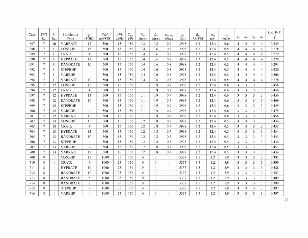
73
Case
PVT Set
kr
Set
Simulation
Type
qoi
(STBD)
GORi
(scf/STB)
APIi (API)
TRes (oF)
Swi
(frac.)
Soi
(frac.)
kro,end (frac.)
pi
(psi)
Boi
(RB/STB)
oi (cp)
oi
(md/cp)
nw
nw
ng
ng
(Eq. B-1)
687 7 10 VARRATE 12 500 15 150 0.2 0.8 0.9 3998 1.2 12.4 0.6 4 4 4 4 0.329
688 7 11 CONBHP 15 500 15 150 0.4 0.6 0.8 3998 1.2 12.4 0.5 4 4 4 4 0.278
689 7 11 CRATE 4 500 15 150 0.4 0.6 0.8 3998 1.2 12.4 0.5 4 4 4 4 0.279
690 7 11 HYPRATE 17 500 15 150 0.4 0.6 0.8 3998 1.2 12.4 0.5 4 4 4 4 0.278
691 7 11 RANDRATE 10 500 15 150 0.4 0.6 0.8 3998 1.2 12.4 0.5 4 4 4 4 0.294
692 7 11 STEPBHP - 500 15 150 0.4 0.6 0.8 3998 1.2 12.4 0.5 4 4 4 4 0.280
693 7 11 VARBHP - 500 15 150 0.4 0.6 0.8 3998 1.2 12.4 0.5 4 4 4 4 0.300
694 7 11 VARRATE 12 500 15 150 0.4 0.6 0.8 3998 1.2 12.4 0.5 4 4 4 4 0.278
695 7 12 CONBHP 15 500 15 150 0.1 0.9 0.9 3998 1.2 12.4 0.6 3 3 3 3 0.456
696 7 12 CRATE 4 500 15 150 0.1 0.9 0.9 3998 1.2 12.4 0.6 3 3 3 3 0.458
697 7 12 HYPRATE 13 500 15 150 0.1 0.9 0.9 3998 1.2 12.4 0.6 3 3 3 3 0.456
698 7 12 RANDRATE 10 500 15 150 0.1 0.9 0.9 3998 1.2 12.4 0.6 3 3 3 3 0.469
699 7 12 STEPBHP - 500 15 150 0.1 0.9 0.9 3998 1.2 12.4 0.6 3 3 3 3 0.459
700 7 12 VARBHP - 500 15 150 0.1 0.9 0.9 3998 1.2 12.4 0.6 3 3 3 3 0.475
701 7 12 VARRATE 12 500 15 150 0.1 0.9 0.9 3998 1.2 12.4 0.6 3 3 3 3 0.456
702 7 13 CONBHP 15 500 15 150 0.2 0.8 0.7 3998 1.2 12.4 0.5 3 3 3 3 0.434
703 7 13 CRATE 4 500 15 150 0.2 0.8 0.7 3998 1.2 12.4 0.5 3 3 3 3 0.432
704 7 13 HYPRATE 13 500 15 150 0.2 0.8 0.7 3998 1.2 12.4 0.5 3 3 3 3 0.434
705 7 13 RANDRATE 10 500 15 150 0.2 0.8 0.7 3998 1.2 12.4 0.5 3 3 3 3 0.445
706 7 13 STEPBHP - 500 15 150 0.2 0.8 0.7 3998 1.2 12.4 0.5 3 3 3 3 0.434
707 7 13 VARBHP - 500 15 150 0.2 0.8 0.7 3998 1.2 12.4 0.5 3 3 3 3 0.453
708 7 13 VARRATE 12 500 15 150 0.2 0.8 0.7 3998 1.2 12.4 0.5 3 3 3 3 0.434
709 8 1 CONBHP 15 1000 25 150 0 1 1 5337 1.5 1.2 5.9 3 3 3 3 0.392
710 8 1 CRATE 4 1000 25 150 0 1 1 5337 1.5 1.2 5.9 3 3 3 3 0.390
711 8 1 HYPRATE 10 1000 25 150 0 1 1 5337 1.5 1.2 5.9 3 3 3 3 0.388
712 8 1 RANDRATE 10 1000 25 150 0 1 1 5337 1.5 1.2 5.9 3 3 3 3 0.387
713 8 1 RANDRATE 5 1000 25 150 0 1 1 5337 1.5 1.2 5.9 3 3 3 3 0.409
714 8 1 RANDRATE 8 1000 25 150 0 1 1 5337 1.5 1.2 5.9 3 3 3 3 0.389
715 8 1 STEPBHP - 1000 25 150 0 1 1 5337 1.5 1.2 5.9 3 3 3 3 0.397
716 8 1 VARBHP - 1000 25 150 0 1 1 5337 1.5 1.2 5.9 3 3 3 3 0.397

74
Case
PVT Set
kr
Set
Simulation
Type
qoi
(STBD)
GORi
(scf/STB)
APIi (API)
TRes (oF)
Swi
(frac.)
Soi
(frac.)
kro,end (frac.)
pi
(psi)
Boi
(RB/STB)
oi (cp)
oi
(md/cp)
nw
nw
ng
ng
(Eq. B-1)
717 8 1 VARRATE 12 1000 25 150 0 1 1 5337 1.5 1.2 5.9 3 3 3 3 0.387
718 8 2 CONBHP 15 1000 25 150 0.2 0.8 0.9 5337 1.5 1.2 5.3 3 3 3 3 0.354
719 8 2 CRATE 2 1000 25 150 0.2 0.8 0.9 5337 1.5 1.2 5.3 3 3 3 3 0.356
720 8 2 CRATE 4 1000 25 150 0.2 0.8 0.9 5337 1.5 1.2 5.3 3 3 3 3 0.348
721 8 2 HYPRATE 10 1000 25 150 0.2 0.8 0.9 5337 1.5 1.2 5.3 3 3 3 3 0.348
722 8 2 HYPRATE 5 1000 25 150 0.2 0.8 0.9 5337 1.5 1.2 5.3 3 3 3 3 0.350
723 8 2 RANDRATE 10 1000 25 150 0.2 0.8 0.9 5337 1.5 1.2 5.3 3 3 3 3 0.348
724 8 2 RANDRATE 5 1000 25 150 0.2 0.8 0.9 5337 1.5 1.2 5.3 3 3 3 3 0.350
725 8 2 RANDRATE 8 1000 25 150 0.2 0.8 0.9 5337 1.5 1.2 5.3 3 3 3 3 0.348
726 8 2 STEPBHP - 1000 25 150 0.2 0.8 0.9 5337 1.5 1.2 5.3 3 3 3 3 0.357
727 8 2 VARBHP - 1000 25 150 0.2 0.8 0.9 5337 1.5 1.2 5.3 3 3 3 3 0.358
728 8 2 VARRATE 12 1000 25 150 0.2 0.8 0.9 5337 1.5 1.2 5.3 3 3 3 3 0.349
729 8 3 CONBHP 15 1000 25 150 0.4 0.6 0.8 5337 1.5 1.2 4.7 3 3 3 3 0.311
730 8 3 CRATE 2 1000 25 150 0.4 0.6 0.8 5337 1.5 1.2 4.7 3 3 3 3 0.303
731 8 3 CRATE 4 1000 25 150 0.4 0.6 0.8 5337 1.5 1.2 4.7 3 3 3 3 0.302
732 8 3 HYPRATE 10 1000 25 150 0.4 0.6 0.8 5337 1.5 1.2 4.7 3 3 3 3 0.303
733 8 3 HYPRATE 5 1000 25 150 0.4 0.6 0.8 5337 1.5 1.2 4.7 3 3 3 3 0.302
734 8 3 RANDRATE 10 1000 25 150 0.4 0.6 0.8 5337 1.5 1.2 4.7 3 3 3 3 0.303
735 8 3 RANDRATE 5 1000 25 150 0.4 0.6 0.8 5337 1.5 1.2 4.7 3 3 3 3 0.302
736 8 3 RANDRATE 8 1000 25 150 0.4 0.6 0.8 5337 1.5 1.2 4.7 3 3 3 3 0.302
737 8 3 STEPBHP - 1000 25 150 0.4 0.6 0.8 5337 1.5 1.2 4.7 3 3 3 3 0.311
738 8 3 VARBHP - 1000 25 150 0.4 0.6 0.8 5337 1.5 1.2 4.7 3 3 3 3 0.313
739 8 3 VARRATE 12 1000 25 150 0.4 0.6 0.8 5337 1.5 1.2 4.7 3 3 3 3 0.304
740 8 3 VARRATE 5 1000 25 150 0.4 0.6 0.8 5337 1.5 1.2 4.7 3 3 3 3 0.303
741 8 4 CONBHP 15 1000 25 150 0 1 1 5337 1.5 1.2 5.9 3 3 4 3 0.300
742 8 4 CRATE 4 1000 25 150 0 1 1 5337 1.5 1.2 5.9 3 3 4 3 0.297
743 8 4 HYPRATE 10 1000 25 150 0 1 1 5337 1.5 1.2 5.9 3 3 4 3 0.295
744 8 4 RANDRATE 10 1000 25 150 0 1 1 5337 1.5 1.2 5.9 3 3 4 3 0.296
745 8 4 RANDRATE 5 1000 25 150 0 1 1 5337 1.5 1.2 5.9 3 3 4 3 0.307
746 8 4 RANDRATE 8 1000 25 150 0 1 1 5337 1.5 1.2 5.9 3 3 4 3 0.297

75
Case
PVT Set
kr
Set
Simulation
Type
qoi
(STBD)
GORi
(scf/STB)
APIi (API)
TRes (oF)
Swi
(frac.)
Soi
(frac.)
kro,end (frac.)
pi
(psi)
Boi
(RB/STB)
oi (cp)
oi
(md/cp)
nw
nw
ng
ng
(Eq. B-1)
747 8 4 STEPBHP - 1000 25 150 0 1 1 5337 1.5 1.2 5.9 3 3 4 3 0.305
748 8 4 VARBHP - 1000 25 150 0 1 1 5337 1.5 1.2 5.9 3 3 4 3 0.305
749 8 4 VARRATE 10 1000 25 150 0 1 1 5337 1.5 1.2 5.9 3 3 4 3 0.295
750 8 4 VARRATE 12 1000 25 150 0 1 1 5337 1.5 1.2 5.9 3 3 4 3 0.295
751 8 5 CONBHP 15 1000 25 150 0.4 0.6 0.8 5337 1.5 1.2 4.7 3 3 4 3 0.207
752 8 5 CRATE 2 1000 25 150 0.4 0.6 0.8 5337 1.5 1.2 4.7 3 3 4 3 0.201
753 8 5 CRATE 4 1000 25 150 0.4 0.6 0.8 5337 1.5 1.2 4.7 3 3 4 3 0.201
754 8 5 HYPRATE 10 1000 25 150 0.4 0.6 0.8 5337 1.5 1.2 4.7 3 3 4 3 0.202
755 8 5 HYPRATE 5 1000 25 150 0.4 0.6 0.8 5337 1.5 1.2 4.7 3 3 4 3 0.201
756 8 5 RANDRATE 10 1000 25 150 0.4 0.6 0.8 5337 1.5 1.2 4.7 3 3 4 3 0.202
757 8 5 RANDRATE 5 1000 25 150 0.4 0.6 0.8 5337 1.5 1.2 4.7 3 3 4 3 0.201
758 8 5 RANDRATE 6 1000 25 150 0.4 0.6 0.8 5337 1.5 1.2 4.7 3 3 4 3 0.201
759 8 5 RANDRATE 8 1000 25 150 0.4 0.6 0.8 5337 1.5 1.2 4.7 3 3 4 3 0.201
760 8 5 STEPBHP - 1000 25 150 0.4 0.6 0.8 5337 1.5 1.2 4.7 3 3 4 3 0.209
761 8 5 VARBHP - 1000 25 150 0.4 0.6 0.8 5337 1.5 1.2 4.7 3 3 4 3 0.209
762 8 5 VARRATE 10 1000 25 150 0.4 0.6 0.8 5337 1.5 1.2 4.7 3 3 4 3 0.203
763 8 5 VARRATE 12 1000 25 150 0.4 0.6 0.8 5337 1.5 1.2 4.7 3 3 4 3 0.203
764 8 5 VARRATE 5 1000 25 150 0.4 0.6 0.8 5337 1.5 1.2 4.7 3 3 4 3 0.201
765 8 6 CONBHP 15 1000 25 150 0 1 1 5337 1.5 1.2 5.9 2 2 2 2 0.550
766 8 6 CRATE 4 1000 25 150 0 1 1 5337 1.5 1.2 5.9 2 2 2 2 0.544
767 8 6 RANDRATE 8 1000 25 150 0 1 1 5337 1.5 1.2 5.9 2 2 2 2 0.545
768 8 6 STEPBHP - 1000 25 150 0 1 1 5337 1.5 1.2 5.9 2 2 2 2 0.547
769 8 6 VARBHP - 1000 25 150 0 1 1 5337 1.5 1.2 5.9 2 2 2 2 0.553
770 8 6 VARRATE 12 1000 25 150 0 1 1 5337 1.5 1.2 5.9 2 2 2 2 0.545
771 8 7 CONBHP 15 1000 25 150 0.2 0.8 0.9 5337 1.5 1.2 5.3 2 2 2 2 0.603
772 8 7 CRATE 4 1000 25 150 0.2 0.8 0.9 5337 1.5 1.2 5.3 2 2 2 2 0.598
773 8 7 STEPBHP - 1000 25 150 0.2 0.8 0.9 5337 1.5 1.2 5.3 2 2 2 2 0.599
774 8 7 VARBHP - 1000 25 150 0.2 0.8 0.9 5337 1.5 1.2 5.3 2 2 2 2 0.604
775 8 7 VARRATE 12 1000 25 150 0.2 0.8 0.9 5337 1.5 1.2 5.3 2 2 2 2 0.599
776 8 8 CONBHP 15 1000 25 150 0.4 0.6 0.8 5337 1.5 1.2 4.7 2 2 2 2 0.484

76
Case
PVT Set
kr
Set
Simulation
Type
qoi
(STBD)
GORi
(scf/STB)
APIi (API)
TRes (oF)
Swi
(frac.)
Soi
(frac.)
kro,end (frac.)
pi
(psi)
Boi
(RB/STB)
oi (cp)
oi
(md/cp)
nw
nw
ng
ng
(Eq. B-1)
777 8 8 CRATE 4 1000 25 150 0.4 0.6 0.8 5337 1.5 1.2 4.7 2 2 2 2 0.477
778 8 8 HYPRATE 13 1000 25 150 0.4 0.6 0.8 5337 1.5 1.2 4.7 2 2 2 2 0.478
779 8 8 RANDRATE 10 1000 25 150 0.4 0.6 0.8 5337 1.5 1.2 4.7 2 2 2 2 0.477
780 8 8 STEPBHP - 1000 25 150 0.4 0.6 0.8 5337 1.5 1.2 4.7 2 2 2 2 0.479
781 8 8 VARBHP - 1000 25 150 0.4 0.6 0.8 5337 1.5 1.2 4.7 2 2 2 2 0.484
782 8 8 VARRATE 12 1000 25 150 0.4 0.6 0.8 5337 1.5 1.2 4.7 2 2 2 2 0.478
783 8 9 CONBHP 15 1000 25 150 0 1 1 5337 1.5 1.2 5.9 4 4 4 4 0.261
784 8 9 CRATE 4 1000 25 150 0 1 1 5337 1.5 1.2 5.9 4 4 4 4 0.259
785 8 9 HYPRATE 17 1000 25 150 0 1 1 5337 1.5 1.2 5.9 4 4 4 4 0.256
786 8 9 RANDRATE 8 1000 25 150 0 1 1 5337 1.5 1.2 5.9 4 4 4 4 0.268
787 8 9 STEPBHP - 1000 25 150 0 1 1 5337 1.5 1.2 5.9 4 4 4 4 0.259
788 8 9 VARBHP - 1000 25 150 0 1 1 5337 1.5 1.2 5.9 4 4 4 4 0.272
789 8 9 VARRATE 12 1000 25 150 0 1 1 5337 1.5 1.2 5.9 4 4 4 4 0.258
790 8 10 CONBHP 15 1000 25 150 0.2 0.8 0.9 5337 1.5 1.2 5.3 4 4 4 4 0.226
791 8 10 CRATE 4 1000 25 150 0.2 0.8 0.9 5337 1.5 1.2 5.3 4 4 4 4 0.224
792 8 10 HYPRATE 17 1000 25 150 0.2 0.8 0.9 5337 1.5 1.2 5.3 4 4 4 4 0.224
793 8 10 RANDRATE 10 1000 25 150 0.2 0.8 0.9 5337 1.5 1.2 5.3 4 4 4 4 0.227
794 8 10 STEPBHP - 1000 25 150 0.2 0.8 0.9 5337 1.5 1.2 5.3 4 4 4 4 0.225
795 8 10 VARBHP - 1000 25 150 0.2 0.8 0.9 5337 1.5 1.2 5.3 4 4 4 4 0.234
796 8 10 VARRATE 12 1000 25 150 0.2 0.8 0.9 5337 1.5 1.2 5.3 4 4 4 4 0.223
797 8 11 CONBHP 15 1000 25 150 0.4 0.6 0.8 5337 1.5 1.2 4.7 4 4 4 4 0.172
798 8 11 CRATE 4 1000 25 150 0.4 0.6 0.8 5337 1.5 1.2 4.7 4 4 4 4 0.169
799 8 11 HYPRATE 17 1000 25 150 0.4 0.6 0.8 5337 1.5 1.2 4.7 4 4 4 4 0.171
800 8 11 RANDRATE 10 1000 25 150 0.4 0.6 0.8 5337 1.5 1.2 4.7 4 4 4 4 0.171
801 8 11 STEPBHP - 1000 25 150 0.4 0.6 0.8 5337 1.5 1.2 4.7 4 4 4 4 0.171
802 8 11 VARBHP - 1000 25 150 0.4 0.6 0.8 5337 1.5 1.2 4.7 4 4 4 4 0.180
803 8 11 VARRATE 12 1000 25 150 0.4 0.6 0.8 5337 1.5 1.2 4.7 4 4 4 4 0.171
804 8 12 CONBHP 15 1000 25 150 0.1 0.9 0.9 5337 1.5 1.2 5.3 3 3 3 3 0.391
805 8 12 CRATE 4 1000 25 150 0.1 0.9 0.9 5337 1.5 1.2 5.3 3 3 3 3 0.385
806 8 12 HYPRATE 13 1000 25 150 0.1 0.9 0.9 5337 1.5 1.2 5.3 3 3 3 3 0.385

77
Case
PVT Set
kr
Set
Simulation
Type
qoi
(STBD)
GORi
(scf/STB)
APIi (API)
TRes (oF)
Swi
(frac.)
Soi
(frac.)
kro,end (frac.)
pi
(psi)
Boi
(RB/STB)
oi (cp)
oi
(md/cp)
nw
nw
ng
ng
(Eq. B-1)
807 8 12 RANDRATE 10 1000 25 150 0.1 0.9 0.9 5337 1.5 1.2 5.3 3 3 3 3 0.387
808 8 12 STEPBHP - 1000 25 150 0.1 0.9 0.9 5337 1.5 1.2 5.3 3 3 3 3 0.388
809 8 12 VARBHP - 1000 25 150 0.1 0.9 0.9 5337 1.5 1.2 5.3 3 3 3 3 0.398
810 8 12 VARRATE 12 1000 25 150 0.1 0.9 0.9 5337 1.5 1.2 5.3 3 3 3 3 0.385
811 8 13 CONBHP 15 1000 25 150 0.2 0.8 0.7 5337 1.5 1.2 4.1 3 3 3 3 0.354
812 8 13 CRATE 4 1000 25 150 0.2 0.8 0.7 5337 1.5 1.2 4.1 3 3 3 3 0.347
813 8 13 HYPRATE 13 1000 25 150 0.2 0.8 0.7 5337 1.5 1.2 4.1 3 3 3 3 0.348
814 8 13 RANDRATE 10 1000 25 150 0.2 0.8 0.7 5337 1.5 1.2 4.1 3 3 3 3 0.350
815 8 13 STEPBHP - 1000 25 150 0.2 0.8 0.7 5337 1.5 1.2 4.1 3 3 3 3 0.350
816 8 13 VARBHP - 1000 25 150 0.2 0.8 0.7 5337 1.5 1.2 4.1 3 3 3 3 0.360
817 8 13 VARRATE 12 1000 25 150 0.2 0.8 0.7 5337 1.5 1.2 4.1 3 3 3 3 0.349
818 9 1 CONBHP 15 1500 35 150 0 1 1 5605 1.8 0.4 14.9 3 3 3 3 0.408
819 9 1 CRATE 4 1500 35 150 0 1 1 5605 1.8 0.4 14.9 3 3 3 3 0.402
820 9 1 HYPRATE 10 1500 35 150 0 1 1 5605 1.8 0.4 14.9 3 3 3 3 0.401
821 9 1 HYPRATE 12 1500 35 150 0 1 1 5605 1.8 0.4 14.9 3 3 3 3 0.400
822 9 1 HYPRATE 8 1500 35 150 0 1 1 5605 1.8 0.4 14.9 3 3 3 3 0.437
823 9 1 RANDRATE 6 1500 35 150 0 1 1 5605 1.8 0.4 14.9 3 3 3 3 0.407
824 9 1 RANDRATE 8 1500 35 150 0 1 1 5605 1.8 0.4 14.9 3 3 3 3 0.401
825 9 1 STEPBHP - 1500 35 150 0 1 1 5605 1.8 0.4 14.9 3 3 3 3 0.409
826 9 1 VARBHP - 1500 35 150 0 1 1 5605 1.8 0.4 14.9 3 3 3 3 0.409
827 9 1 VARRATE 10 1500 35 150 0 1 1 5605 1.8 0.4 14.9 3 3 3 3 0.399
828 9 1 VARRATE 12 1500 35 150 0 1 1 5605 1.8 0.4 14.9 3 3 3 3 0.399
829 9 2 CONBHP 15 1500 35 150 0.2 0.8 0.9 5605 1.8 0.4 13.4 3 3 3 3 0.352
830 9 2 CRATE 2 1500 35 150 0.2 0.8 0.9 5605 1.8 0.4 13.4 3 3 3 3 0.350
831 9 2 CRATE 4 1500 35 150 0.2 0.8 0.9 5605 1.8 0.4 13.4 3 3 3 3 0.343
832 9 2 HYPRATE 10 1500 35 150 0.2 0.8 0.9 5605 1.8 0.4 13.4 3 3 3 3 0.342
833 9 2 HYPRATE 12 1500 35 150 0.2 0.8 0.9 5605 1.8 0.4 13.4 3 3 3 3 0.342
834 9 2 HYPRATE 8 1500 35 150 0.2 0.8 0.9 5605 1.8 0.4 13.4 3 3 3 3 0.342
835 9 2 RANDRATE 4 1500 35 150 0.2 0.8 0.9 5605 1.8 0.4 13.4 3 3 3 3 0.347
836 9 2 RANDRATE 6 1500 35 150 0.2 0.8 0.9 5605 1.8 0.4 13.4 3 3 3 3 0.343
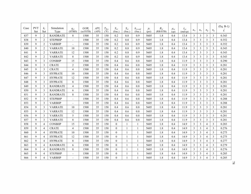
78
Case
PVT Set
kr
Set
Simulation
Type
qoi
(STBD)
GORi
(scf/STB)
APIi (API)
TRes (oF)
Swi
(frac.)
Soi
(frac.)
kro,end (frac.)
pi
(psi)
Boi
(RB/STB)
oi (cp)
oi
(md/cp)
nw
nw
ng
ng
(Eq. B-1)
837 9 2 RANDRATE 8 1500 35 150 0.2 0.8 0.9 5605 1.8 0.4 13.4 3 3 3 3 0.343
838 9 2 STEPBHP - 1500 35 150 0.2 0.8 0.9 5605 1.8 0.4 13.4 3 3 3 3 0.352
839 9 2 VARBHP - 1500 35 150 0.2 0.8 0.9 5605 1.8 0.4 13.4 3 3 3 3 0.352
840 9 2 VARRATE 10 1500 35 150 0.2 0.8 0.9 5605 1.8 0.4 13.4 3 3 3 3 0.343
841 9 2 VARRATE 12 1500 35 150 0.2 0.8 0.9 5605 1.8 0.4 13.4 3 3 3 3 0.343
842 9 2 VARRATE 8 1500 35 150 0.2 0.8 0.9 5605 1.8 0.4 13.4 3 3 3 3 0.343
843 9 3 CONBHP 15 1500 35 150 0.4 0.6 0.8 5605 1.8 0.4 11.9 3 3 3 3 0.290
844 9 3 CRATE 2 1500 35 150 0.4 0.6 0.8 5605 1.8 0.4 11.9 3 3 3 3 0.281
845 9 3 CRATE 4 1500 35 150 0.4 0.6 0.8 5605 1.8 0.4 11.9 3 3 3 3 0.281
846 9 3 HYPRATE 10 1500 35 150 0.4 0.6 0.8 5605 1.8 0.4 11.9 3 3 3 3 0.281
847 9 3 HYPRATE 12 1500 35 150 0.4 0.6 0.8 5605 1.8 0.4 11.9 3 3 3 3 0.281
848 9 3 HYPRATE 8 1500 35 150 0.4 0.6 0.8 5605 1.8 0.4 11.9 3 3 3 3 0.281
849 9 3 RANDRATE 4 1500 35 150 0.4 0.6 0.8 5605 1.8 0.4 11.9 3 3 3 3 0.281
850 9 3 RANDRATE 6 1500 35 150 0.4 0.6 0.8 5605 1.8 0.4 11.9 3 3 3 3 0.281
851 9 3 RANDRATE 8 1500 35 150 0.4 0.6 0.8 5605 1.8 0.4 11.9 3 3 3 3 0.281
852 9 3 STEPBHP - 1500 35 150 0.4 0.6 0.8 5605 1.8 0.4 11.9 3 3 3 3 0.288
853 9 3 VARBHP - 1500 35 150 0.4 0.6 0.8 5605 1.8 0.4 11.9 3 3 3 3 0.288
854 9 3 VARRATE 10 1500 35 150 0.4 0.6 0.8 5605 1.8 0.4 11.9 3 3 3 3 0.281
855 9 3 VARRATE 12 1500 35 150 0.4 0.6 0.8 5605 1.8 0.4 11.9 3 3 3 3 0.281
856 9 3 VARRATE 5 1500 35 150 0.4 0.6 0.8 5605 1.8 0.4 11.9 3 3 3 3 0.281
857 9 3 VARRATE 8 1500 35 150 0.4 0.6 0.8 5605 1.8 0.4 11.9 3 3 3 3 0.281
858 9 4 CONBHP 15 1500 35 150 0 1 1 5605 1.8 0.4 14.9 3 3 4 3 0.283
859 9 4 CRATE 4 1500 35 150 0 1 1 5605 1.8 0.4 14.9 3 3 4 3 0.276
860 9 4 HYPRATE 10 1500 35 150 0 1 1 5605 1.8 0.4 14.9 3 3 4 3 0.275
861 9 4 HYPRATE 12 1500 35 150 0 1 1 5605 1.8 0.4 14.9 3 3 4 3 0.275
862 9 4 HYPRATE 8 1500 35 150 0 1 1 5605 1.8 0.4 14.9 3 3 4 3 0.277
863 9 4 RANDRATE 6 1500 35 150 0 1 1 5605 1.8 0.4 14.9 3 3 4 3 0.279
864 9 4 RANDRATE 8 1500 35 150 0 1 1 5605 1.8 0.4 14.9 3 3 4 3 0.276
865 9 4 STEPBHP - 1500 35 150 0 1 1 5605 1.8 0.4 14.9 3 3 4 3 0.285
866 9 4 VARBHP - 1500 35 150 0 1 1 5605 1.8 0.4 14.9 3 3 4 3 0.285

79
Case
PVT Set
kr
Set
Simulation
Type
qoi
(STBD)
GORi
(scf/STB)
APIi (API)
TRes (oF)
Swi
(frac.)
Soi
(frac.)
kro,end (frac.)
pi
(psi)
Boi
(RB/STB)
oi (cp)
oi
(md/cp)
nw
nw
ng
ng
(Eq. B-1)
867 9 4 VARRATE 10 1500 35 150 0 1 1 5605 1.8 0.4 14.9 3 3 4 3 0.275
868 9 4 VARRATE 12 1500 35 150 0 1 1 5605 1.8 0.4 14.9 3 3 4 3 0.275
869 9 4 VARRATE 8 1500 35 150 0 1 1 5605 1.8 0.4 14.9 3 3 4 3 0.300
870 9 5 CONBHP 15 1500 35 150 0.4 0.6 0.8 5605 1.8 0.4 11.9 3 3 4 3 0.178
871 9 5 CRATE 2 1500 35 150 0.4 0.6 0.8 5605 1.8 0.4 11.9 3 3 4 3 0.172
872 9 5 CRATE 4 1500 35 150 0.4 0.6 0.8 5605 1.8 0.4 11.9 3 3 4 3 0.172
873 9 5 HYPRATE 10 1500 35 150 0.4 0.6 0.8 5605 1.8 0.4 11.9 3 3 4 3 0.172
874 9 5 HYPRATE 12 1500 35 150 0.4 0.6 0.8 5605 1.8 0.4 11.9 3 3 4 3 0.172
875 9 5 HYPRATE 8 1500 35 150 0.4 0.6 0.8 5605 1.8 0.4 11.9 3 3 4 3 0.172
876 9 5 RANDRATE 4 1500 35 150 0.4 0.6 0.8 5605 1.8 0.4 11.9 3 3 4 3 0.172
877 9 5 RANDRATE 6 1500 35 150 0.4 0.6 0.8 5605 1.8 0.4 11.9 3 3 4 3 0.172
878 9 5 RANDRATE 8 1500 35 150 0.4 0.6 0.8 5605 1.8 0.4 11.9 3 3 4 3 0.172
879 9 5 STEPBHP - 1500 35 150 0.4 0.6 0.8 5605 1.8 0.4 11.9 3 3 4 3 0.178
880 9 5 VARBHP - 1500 35 150 0.4 0.6 0.8 5605 1.8 0.4 11.9 3 3 4 3 0.178
881 9 5 VARRATE 10 1500 35 150 0.4 0.6 0.8 5605 1.8 0.4 11.9 3 3 4 3 0.172
882 9 5 VARRATE 12 1500 35 150 0.4 0.6 0.8 5605 1.8 0.4 11.9 3 3 4 3 0.172
883 9 5 VARRATE 5 1500 35 150 0.4 0.6 0.8 5605 1.8 0.4 11.9 3 3 4 3 0.172
884 9 5 VARRATE 8 1500 35 150 0.4 0.6 0.8 5605 1.8 0.4 11.9 3 3 4 3 0.172
885 9 6 CONBHP 15 1500 35 150 0 1 1 5605 1.8 0.4 14.9 2 2 2 2 0.627
886 9 6 CRATE 4 1500 35 150 0 1 1 5605 1.8 0.4 14.9 2 2 2 2 0.618
887 9 6 RANDRATE 8 1500 35 150 0 1 1 5605 1.8 0.4 14.9 2 2 2 2 0.619
888 9 6 STEPBHP - 1500 35 150 0 1 1 5605 1.8 0.4 14.9 2 2 2 2 0.621
889 9 6 VARBHP - 1500 35 150 0 1 1 5605 1.8 0.4 14.9 2 2 2 2 0.626
890 9 6 VARRATE 12 1500 35 150 0 1 1 5605 1.8 0.4 14.9 2 2 2 2 0.618
891 9 7 CONBHP 15 1500 35 150 0.2 0.8 0.9 5605 1.8 0.4 13.4 2 2 2 2 0.710
892 9 7 CRATE 4 1500 35 150 0.2 0.8 0.9 5605 1.8 0.4 13.4 2 2 2 2 0.702
893 9 7 STEPBHP - 1500 35 150 0.2 0.8 0.9 5605 1.8 0.4 13.4 2 2 2 2 0.704
894 9 7 VARBHP - 1500 35 150 0.2 0.8 0.9 5605 1.8 0.4 13.4 2 2 2 2 0.707
895 9 7 VARRATE 12 1500 35 150 0.2 0.8 0.9 5605 1.8 0.4 13.4 2 2 2 2 0.702
896 9 8 CONBHP 15 1500 35 150 0.4 0.6 0.8 5605 1.8 0.4 11.9 2 2 2 2 0.515

80
Case
PVT Set
kr
Set
Simulation
Type
qoi
(STBD)
GORi
(scf/STB)
APIi (API)
TRes (oF)
Swi
(frac.)
Soi
(frac.)
kro,end (frac.)
pi
(psi)
Boi
(RB/STB)
oi (cp)
oi
(md/cp)
nw
nw
ng
ng
(Eq. B-1)
897 9 8 CRATE 4 1500 35 150 0.4 0.6 0.8 5605 1.8 0.4 11.9 2 2 2 2 0.505
898 9 8 HYPRATE 13 1500 35 150 0.4 0.6 0.8 5605 1.8 0.4 11.9 2 2 2 2 0.506
899 9 8 RANDRATE 10 1500 35 150 0.4 0.6 0.8 5605 1.8 0.4 11.9 2 2 2 2 0.505
900 9 8 STEPBHP - 1500 35 150 0.4 0.6 0.8 5605 1.8 0.4 11.9 2 2 2 2 0.507
901 9 8 VARBHP - 1500 35 150 0.4 0.6 0.8 5605 1.8 0.4 11.9 2 2 2 2 0.511
902 9 8 VARRATE 12 1500 35 150 0.4 0.6 0.8 5605 1.8 0.4 11.9 2 2 2 2 0.505
903 9 9 CONBHP 15 1500 35 150 0 1 1 5605 1.8 0.4 14.9 4 4 4 4 0.246
904 9 9 CRATE 4 1500 35 150 0 1 1 5605 1.8 0.4 14.9 4 4 4 4 0.240
905 9 9 HYPRATE 17 1500 35 150 0 1 1 5605 1.8 0.4 14.9 4 4 4 4 0.239
906 9 9 RANDRATE 8 1500 35 150 0 1 1 5605 1.8 0.4 14.9 4 4 4 4 0.244
907 9 9 STEPBHP - 1500 35 150 0 1 1 5605 1.8 0.4 14.9 4 4 4 4 0.242
908 9 9 VARBHP - 1500 35 150 0 1 1 5605 1.8 0.4 14.9 4 4 4 4 0.253
909 9 9 VARRATE 12 1500 35 150 0 1 1 5605 1.8 0.4 14.9 4 4 4 4 0.240
910 9 10 CONBHP 15 1500 35 150 0.2 0.8 0.9 5605 1.8 0.4 13.4 4 4 4 4 0.201
911 9 10 CRATE 4 1500 35 150 0.2 0.8 0.9 5605 1.8 0.4 13.4 4 4 4 4 0.197
912 9 10 HYPRATE 17 1500 35 150 0.2 0.8 0.9 5605 1.8 0.4 13.4 4 4 4 4 0.197
913 9 10 RANDRATE 10 1500 35 150 0.2 0.8 0.9 5605 1.8 0.4 13.4 4 4 4 4 0.198
914 9 10 STEPBHP - 1500 35 150 0.2 0.8 0.9 5605 1.8 0.4 13.4 4 4 4 4 0.198
915 9 10 VARBHP - 1500 35 150 0.2 0.8 0.9 5605 1.8 0.4 13.4 4 4 4 4 0.204
916 9 10 VARRATE 12 1500 35 150 0.2 0.8 0.9 5605 1.8 0.4 13.4 4 4 4 4 0.197
917 9 11 CONBHP 15 1500 35 150 0.4 0.6 0.8 5605 1.8 0.4 11.9 4 4 4 4 0.154
918 9 11 CRATE 4 1500 35 150 0.4 0.6 0.8 5605 1.8 0.4 11.9 4 4 4 4 0.150
919 9 11 HYPRATE 17 1500 35 150 0.4 0.6 0.8 5605 1.8 0.4 11.9 4 4 4 4 0.151
920 9 11 RANDRATE 10 1500 35 150 0.4 0.6 0.8 5605 1.8 0.4 11.9 4 4 4 4 0.151
921 9 11 STEPBHP - 1500 35 150 0.4 0.6 0.8 5605 1.8 0.4 11.9 4 4 4 4 0.151
922 9 11 VARBHP - 1500 35 150 0.4 0.6 0.8 5605 1.8 0.4 11.9 4 4 4 4 0.157
923 9 11 VARRATE 12 1500 35 150 0.4 0.6 0.8 5605 1.8 0.4 11.9 4 4 4 4 0.151
924 9 12 CONBHP 15 1500 35 150 0.1 0.9 0.9 5605 1.8 0.4 13.4 3 3 3 3 0.407
925 9 12 CRATE 4 1500 35 150 0.1 0.9 0.9 5605 1.8 0.4 13.4 3 3 3 3 0.398
926 9 12 HYPRATE 13 1500 35 150 0.1 0.9 0.9 5605 1.8 0.4 13.4 3 3 3 3 0.398
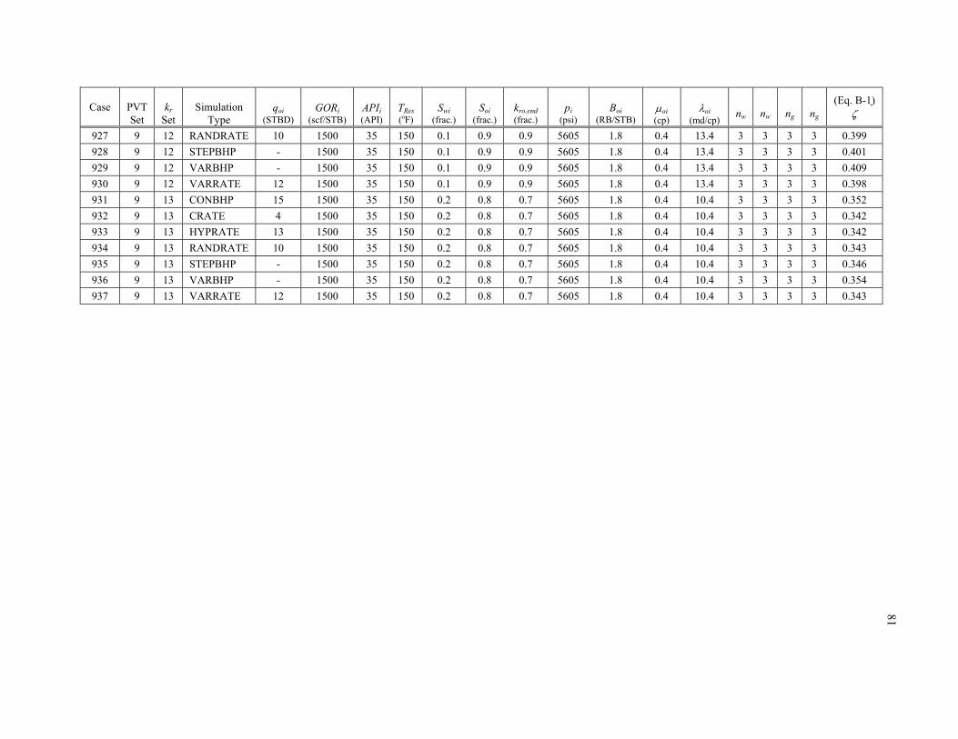
81
Case
PVT Set
kr
Set
Simulation
Type
qoi
(STBD)
GORi
(scf/STB)
APIi (API)
TRes (oF)
Swi
(frac.)
Soi
(frac.)
kro,end (frac.)
pi
(psi)
Boi
(RB/STB)
oi (cp)
oi
(md/cp)
nw
nw
ng
ng
(Eq. B-1)
927 9 12 RANDRATE 10 1500 35 150 0.1 0.9 0.9 5605 1.8 0.4 13.4 3 3 3 3 0.399
928 9 12 STEPBHP - 1500 35 150 0.1 0.9 0.9 5605 1.8 0.4 13.4 3 3 3 3 0.401
929 9 12 VARBHP - 1500 35 150 0.1 0.9 0.9 5605 1.8 0.4 13.4 3 3 3 3 0.409
930 9 12 VARRATE 12 1500 35 150 0.1 0.9 0.9 5605 1.8 0.4 13.4 3 3 3 3 0.398
931 9 13 CONBHP 15 1500 35 150 0.2 0.8 0.7 5605 1.8 0.4 10.4 3 3 3 3 0.352
932 9 13 CRATE 4 1500 35 150 0.2 0.8 0.7 5605 1.8 0.4 10.4 3 3 3 3 0.342
933 9 13 HYPRATE 13 1500 35 150 0.2 0.8 0.7 5605 1.8 0.4 10.4 3 3 3 3 0.342
934 9 13 RANDRATE 10 1500 35 150 0.2 0.8 0.7 5605 1.8 0.4 10.4 3 3 3 3 0.343
935 9 13 STEPBHP - 1500 35 150 0.2 0.8 0.7 5605 1.8 0.4 10.4 3 3 3 3 0.346
936 9 13 VARBHP - 1500 35 150 0.2 0.8 0.7 5605 1.8 0.4 10.4 3 3 3 3 0.354
937 9 13 VARRATE 12 1500 35 150 0.2 0.8 0.7 5605 1.8 0.4 10.4 3 3 3 3 0.343

82
APPENDIX C
CORRELATION PLOTS FOR THE CUBIC MODEL (CASE 1)
Figure C.1 — Normalized oil-phase mobility function plotted versus the normalized average reservoir pressure function (Case 1).
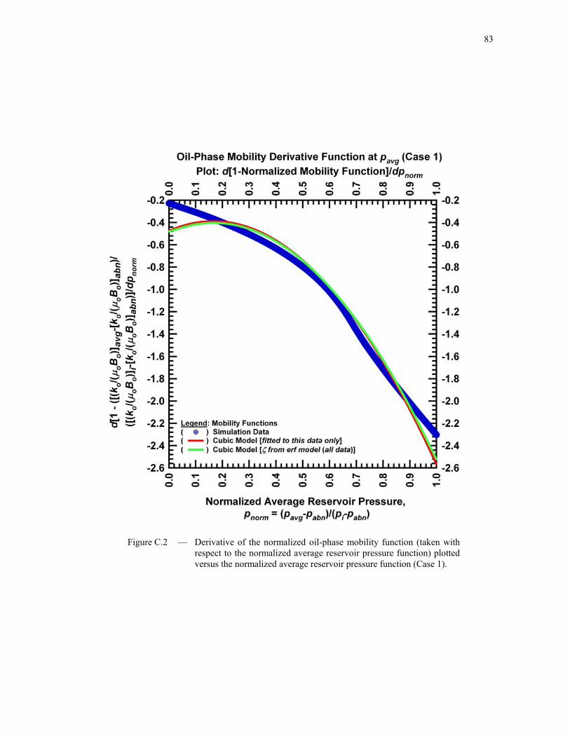
83
Figure C.2 — Derivative of the normalized oil-phase mobility function (taken with respect to the normalized average reservoir pressure function) plotted versus the normalized average reservoir pressure function (Case 1).

84
Figure C.3 — Second derivative of the normalized oil-phase mobility function (taken with respect to the normalized average reservoir pressure function) plotted versus the normalized average reservoir pressure function (Case 1).

85
Figure C.4 — Integral of the normalized oil-phase mobility function (taken with respect to the normalized average reservoir pressure function) plotted versus the normalized average reservoir pressure function (Case 1).

86
Figure C.5 — Integral difference of the normalized oil-phase mobility function (taken with respect to the normalized average reservoir pressure function) plotted versus the normalized average reservoir pressure function (Case 1).

87
APPENDIX D
CORRELATION PLOTS FOR THE CUBIC MODEL (CASE 62)
Figure D.1 — Normalized oil-phase mobility function plotted versus the normalized average reservoir pressure function (Case 62).
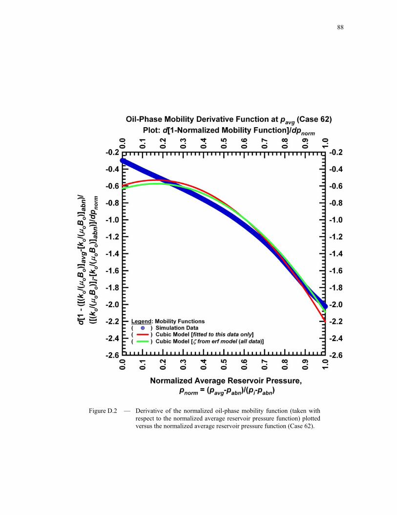
88
Figure D.2 — Derivative of the normalized oil-phase mobility function (taken with respect to the normalized average reservoir pressure function) plotted versus the normalized average reservoir pressure function (Case 62).

89
Figure D.3 — Second derivative of the normalized oil-phase mobility function (taken with respect to the normalized average reservoir pressure function) plotted versus the normalized average reservoir pressure function (Case 62).

90
Figure D.4 — Integral of the normalized oil-phase mobility function (taken with respect to the normalized average reservoir pressure function) plotted versus the normalized average reservoir pressure function (Case 62).

91
Figure D.5 — Integral difference of the normalized oil-phase mobility function (taken with respect to the normalized average reservoir pressure function) plotted versus the normalized average reservoir pressure function (Case 62).

92
APPENDIX E
CORRELATION PLOTS FOR THE CUBIC MODEL (CASE 80)
Figure E.1 — Normalized oil-phase mobility function plotted versus the normalized average reservoir pressure function (Case 80).

93
Figure E.2 — Derivative of the normalized oil-phase mobility function (taken with respect to the normalized average reservoir pressure function) plotted versus the normalized average reservoir pressure function (Case 80).

94
Figure E.3 — Second derivative of the normalized oil-phase mobility function (taken with respect to the normalized average reservoir pressure function) plotted versus the normalized average reservoir pressure function (Case 80).

95
Figure E.4 — Integral of the normalized oil-phase mobility function (taken with respect to the normalized average reservoir pressure function) plotted versus the normalized average reservoir pressure function (Case 80).

96
Figure E.5 — Integral difference of the normalized oil-phase mobility function (taken with respect to the normalized average reservoir pressure function) plotted versus the normalized average reservoir pressure function (Case 80).

97
APPENDIX F
CORRELATION PLOTS FOR THE CUBIC MODEL (CASE 114)
Figure F.1 — Normalized oil-phase mobility function plotted versus the normalized average reservoir pressure function (Case 114).
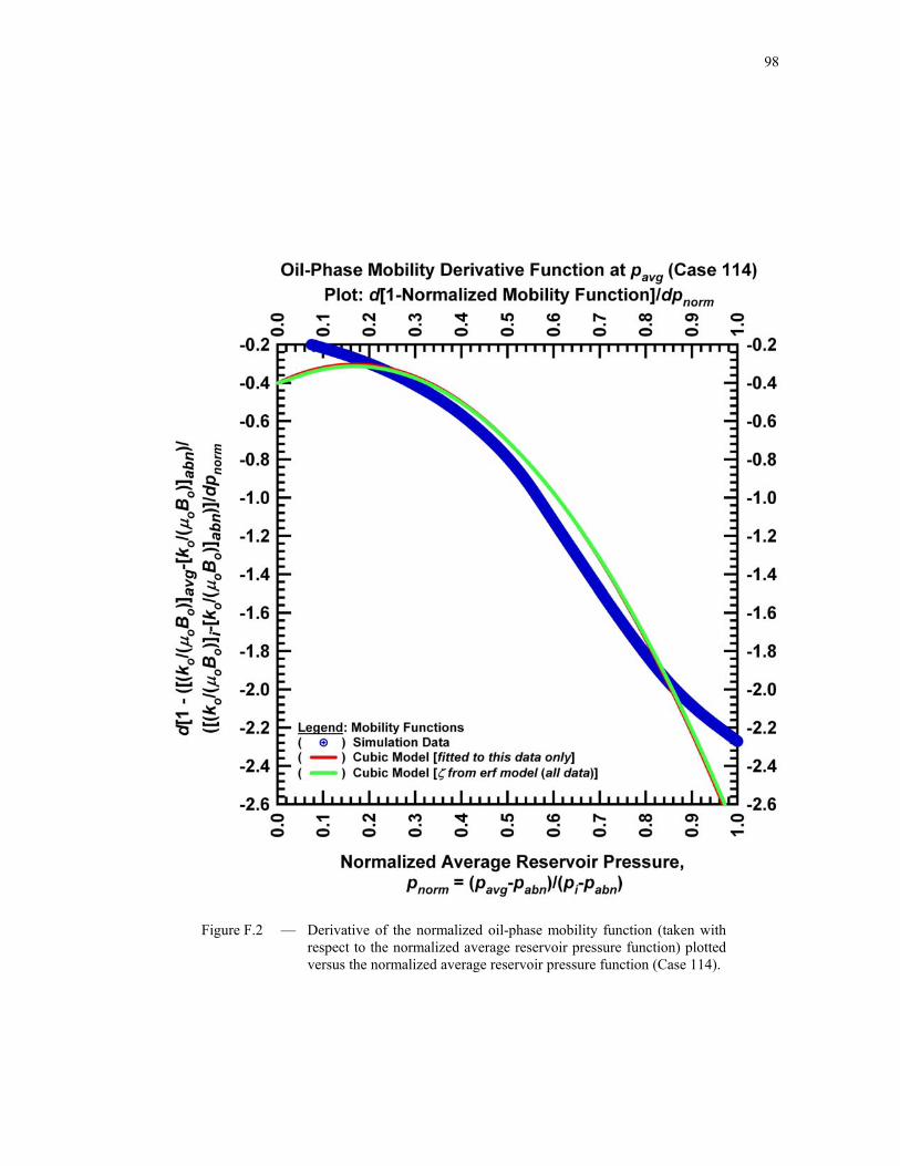
98
Figure F.2 — Derivative of the normalized oil-phase mobility function (taken with respect to the normalized average reservoir pressure function) plotted versus the normalized average reservoir pressure function (Case 114).

99
Figure F.3 — Second derivative of the normalized oil-phase mobility function (taken with respect to the normalized average reservoir pressure function) plotted versus the normalized average reservoir pressure function (Case 114).

100
Figure F.4 — Integral of the normalized oil-phase mobility function (taken with respect to the normalized average reservoir pressure function) plotted versus the normalized average reservoir pressure function (Case 114).
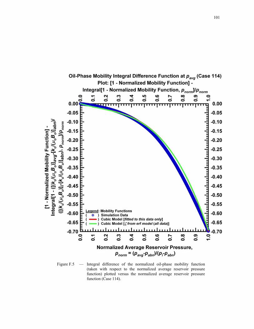
101
Figure F.5 — Integral difference of the normalized oil-phase mobility function (taken with respect to the normalized average reservoir pressure function) plotted versus the normalized average reservoir pressure function (Case 114).

102
APPENDIX G
CORRELATION PLOTS FOR THE CUBIC MODEL (CASE 173)
Figure G.1 — Normalized oil-phase mobility function plotted versus the normalized average reservoir pressure function (Case 173).

103
Figure G.2 — Derivative of the normalized oil-phase mobility function (taken with respect to the normalized average reservoir pressure function) plotted versus the normalized average reservoir pressure function (Case 173).

104
Figure G.3 — Second derivative of the normalized oil-phase mobility function (taken with respect to the normalized average reservoir pressure function) plotted versus the normalized average reservoir pressure function (Case 173).

105
Figure G.4 — Integral of the normalized oil-phase mobility function (taken with respect to the normalized average reservoir pressure function) plotted versus the normalized average reservoir pressure function (Case 173).
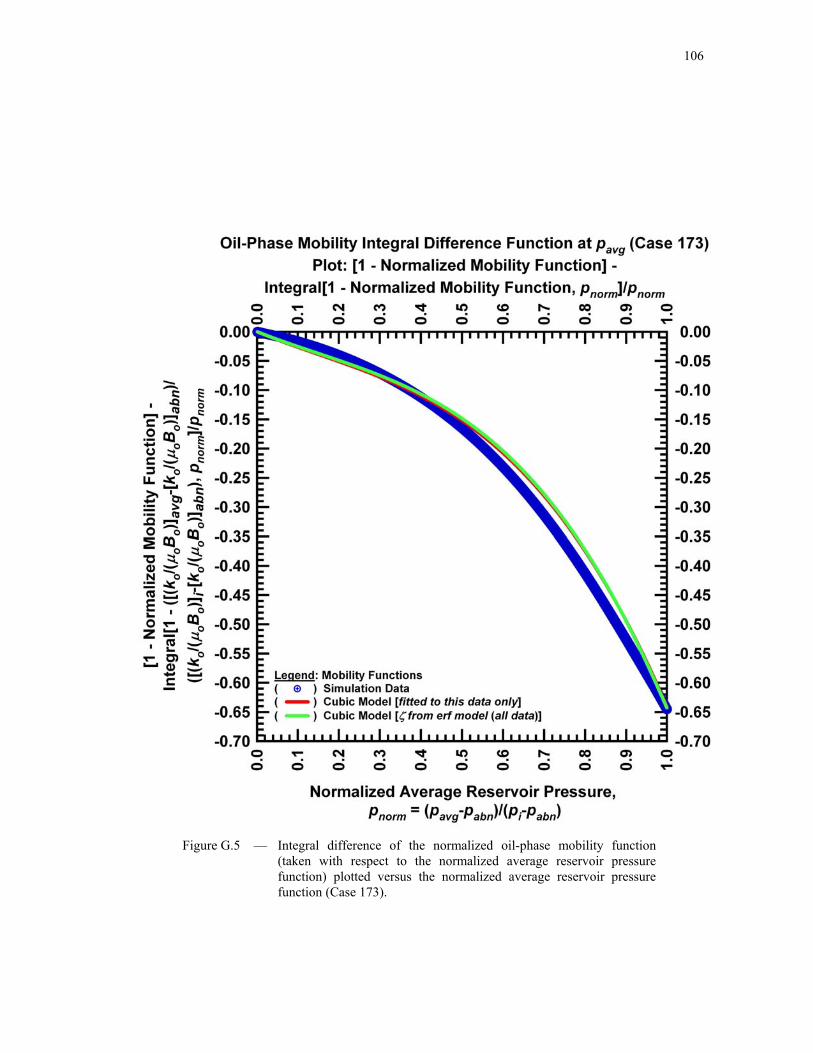
106
Figure G.5 — Integral difference of the normalized oil-phase mobility function (taken with respect to the normalized average reservoir pressure function) plotted versus the normalized average reservoir pressure function (Case 173).

107
APPENDIX H
CORRELATION PLOTS FOR THE CUBIC MODEL (CASE 190)
Figure H.1 — Normalized oil-phase mobility function plotted versus the normalized average reservoir pressure function (Case 190).
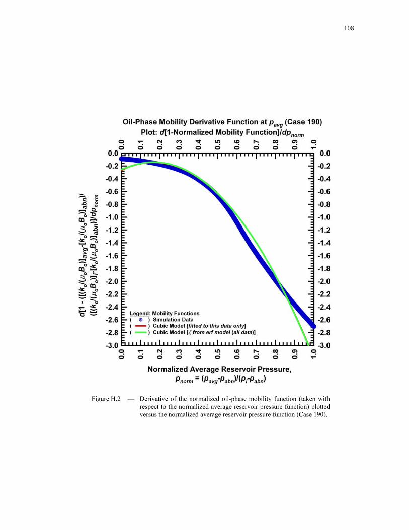
108
Figure H.2 — Derivative of the normalized oil-phase mobility function (taken with respect to the normalized average reservoir pressure function) plotted versus the normalized average reservoir pressure function (Case 190).
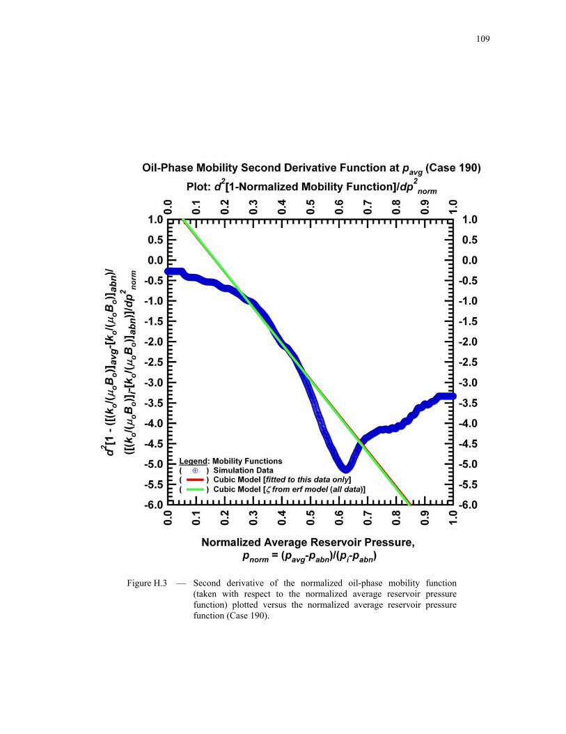
109
Figure H.3 — Second derivative of the normalized oil-phase mobility function (taken with respect to the normalized average reservoir pressure function) plotted versus the normalized average reservoir pressure function (Case 190).

110
Figure H.4 — Integral of the normalized oil-phase mobility function (taken with respect to the normalized average reservoir pressure function) plotted versus the normalized average reservoir pressure function (Case 190).

111
Figure H.5 — Integral difference of the normalized oil-phase mobility function (taken with respect to the normalized average reservoir pressure function) plotted versus the normalized average reservoir pressure function (Case 190).

112
APPENDIX I
CORRELATION PLOTS FOR THE CUBIC MODEL (CASE 505)
Figure I.1 — Normalized oil-phase mobility function plotted versus the normalized average reservoir pressure function (Case 505).
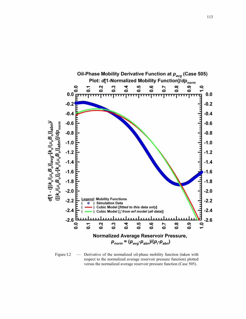
113
Figure I.2 — Derivative of the normalized oil-phase mobility function (taken with respect to the normalized average reservoir pressure function) plotted versus the normalized average reservoir pressure function (Case 505).

114
Figure I.3 — Second derivative of the normalized oil-phase mobility function (taken with respect to the normalized average reservoir pressure function) plotted versus the normalized average reservoir pressure function (Case 505).
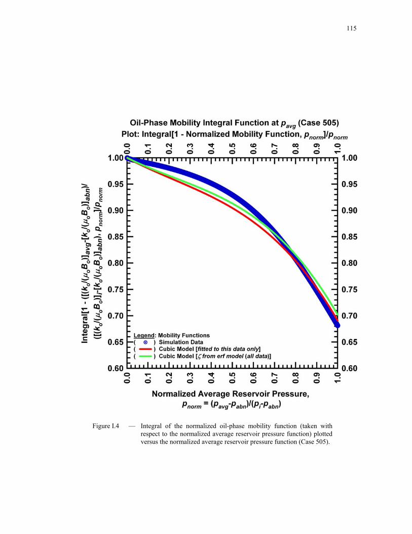
115
Figure I.4 — Integral of the normalized oil-phase mobility function (taken with respect to the normalized average reservoir pressure function) plotted versus the normalized average reservoir pressure function (Case 505).
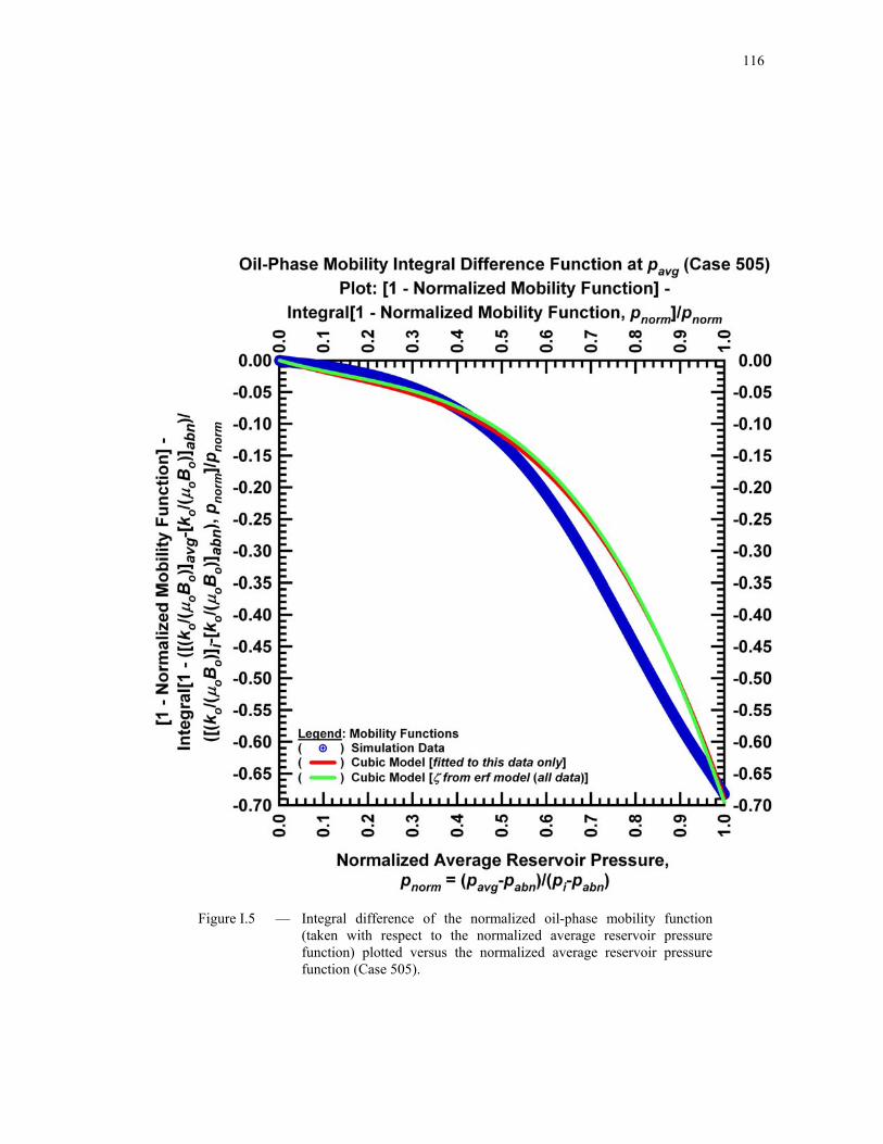
116
Figure I.5 — Integral difference of the normalized oil-phase mobility function (taken with respect to the normalized average reservoir pressure function) plotted versus the normalized average reservoir pressure function (Case 505).
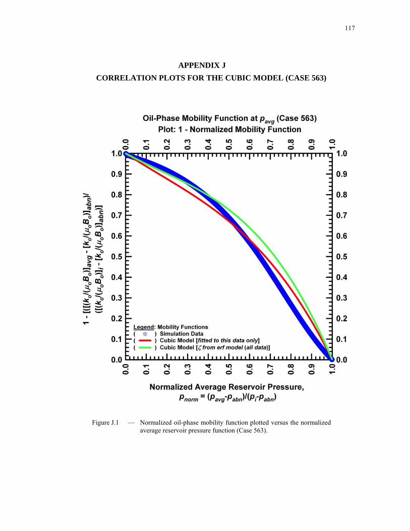
117
APPENDIX J
CORRELATION PLOTS FOR THE CUBIC MODEL (CASE 563)
Figure J.1 — Normalized oil-phase mobility function plotted versus the normalized average reservoir pressure function (Case 563).

118
Figure J.2 — Derivative of the normalized oil-phase mobility function (taken with respect to the normalized average reservoir pressure function) plotted versus the normalized average reservoir pressure function (Case 563).

119
Figure J.3 — Second derivative of the normalized oil-phase mobility function (taken with respect to the normalized average reservoir pressure function) plotted versus the normalized average reservoir pressure function (Case 563).

120
Figure J.4 — Integral of the normalized oil-phase mobility function (taken with respect to the normalized average reservoir pressure function) plotted versus the normalized average reservoir pressure function (Case 563).

121
Figure J.5 — Integral difference of the normalized oil-phase mobility function (taken with respect to the normalized average reservoir pressure function) plotted versus the normalized average reservoir pressure function (Case 563).
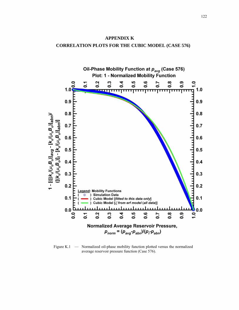
122
APPENDIX K
CORRELATION PLOTS FOR THE CUBIC MODEL (CASE 576)
Figure K.1 — Normalized oil-phase mobility function plotted versus the normalized average reservoir pressure function (Case 576).

123
Figure K.2 — Derivative of the normalized oil-phase mobility function (taken with respect to the normalized average reservoir pressure function) plotted versus the normalized average reservoir pressure function (Case 576).

124
Figure K.3 — Second derivative of the normalized oil-phase mobility function (taken with respect to the normalized average reservoir pressure function) plotted versus the normalized average reservoir pressure function (Case 576).
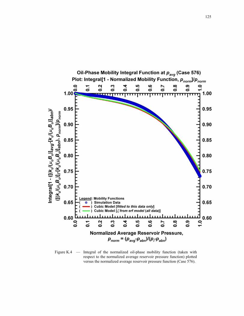
125
Figure K.4 — Integral of the normalized oil-phase mobility function (taken with respect to the normalized average reservoir pressure function) plotted versus the normalized average reservoir pressure function (Case 576).
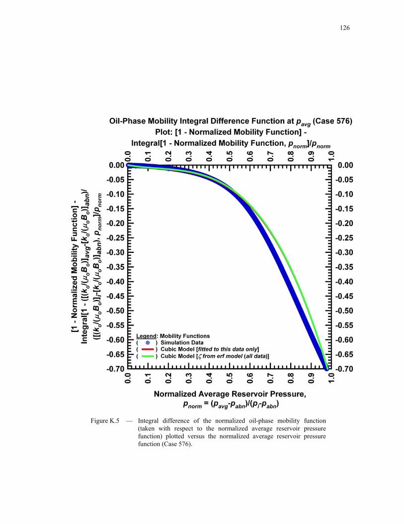
126
Figure K.5 — Integral difference of the normalized oil-phase mobility function (taken with respect to the normalized average reservoir pressure function) plotted versus the normalized average reservoir pressure function (Case 576).

127
APPENDIX L
CORRELATION PLOTS FOR THE CUBIC MODEL (CASE 610)
Figure L.1 — Normalized oil-phase mobility function plotted versus the normalized average reservoir pressure function (Case 610).

128
Figure L.2 — Derivative of the normalized oil-phase mobility function (taken with respect to the normalized average reservoir pressure function) plotted versus the normalized average reservoir pressure function (Case 610).
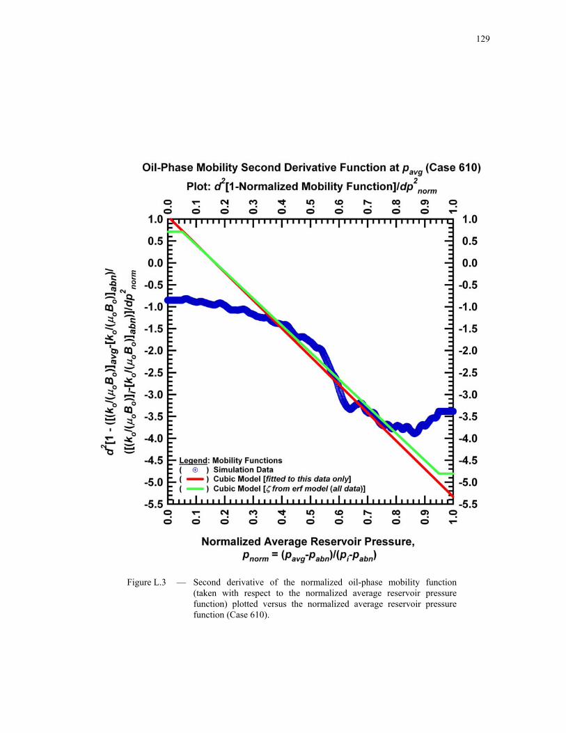
129
Figure L.3 — Second derivative of the normalized oil-phase mobility function (taken with respect to the normalized average reservoir pressure function) plotted versus the normalized average reservoir pressure function (Case 610).

130
Figure L.4 — Integral of the normalized oil-phase mobility function (taken with respect to the normalized average reservoir pressure function) plotted versus the normalized average reservoir pressure function (Case 610).

131
Figure L.5 — Integral difference of the normalized oil-phase mobility function (taken with respect to the normalized average reservoir pressure function) plotted versus the normalized average reservoir pressure function (Case 610).

132
APPENDIX M
CORRELATION PLOTS FOR THE CUBIC MODEL (CASE 660)
Figure M.1 — Normalized oil-phase mobility function plotted versus the normalized average reservoir pressure function (Case 660).

133
Figure M.2 — Derivative of the normalized oil-phase mobility function (taken with respect to the normalized average reservoir pressure function) plotted versus the normalized average reservoir pressure function (Case 660).

134
Figure M.3 — Second derivative of the normalized oil-phase mobility function (taken with respect to the normalized average reservoir pressure function) plotted versus the normalized average reservoir pressure function (Case 660).
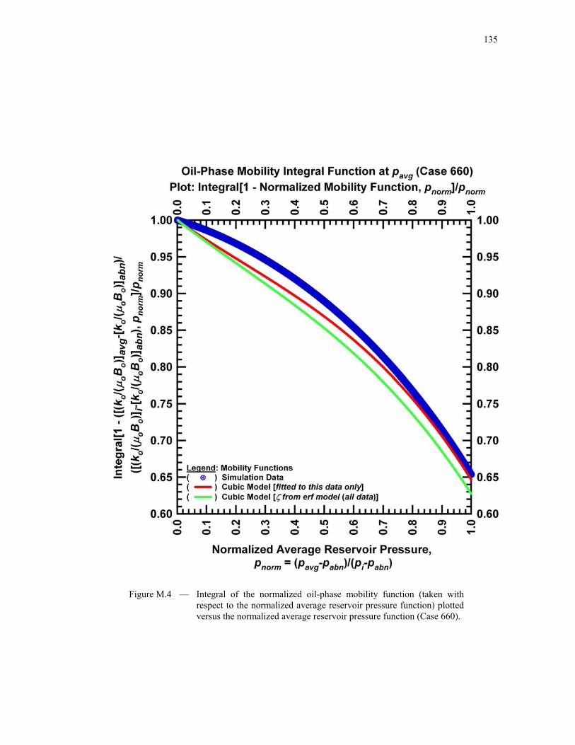
135
Figure M.4 — Integral of the normalized oil-phase mobility function (taken with respect to the normalized average reservoir pressure function) plotted versus the normalized average reservoir pressure function (Case 660).

136
Figure M.5 — Integral difference of the normalized oil-phase mobility function (taken with respect to the normalized average reservoir pressure function) plotted versus the normalized average reservoir pressure function (Case 660).
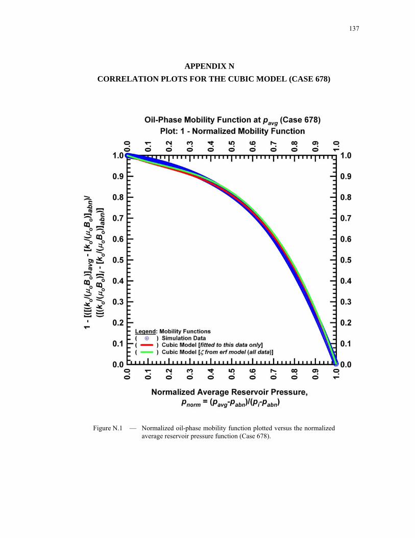
137
APPENDIX N
CORRELATION PLOTS FOR THE CUBIC MODEL (CASE 678)
Figure N.1 — Normalized oil-phase mobility function plotted versus the normalized average reservoir pressure function (Case 678).

138
Figure N.2 — Derivative of the normalized oil-phase mobility function (taken with respect to the normalized average reservoir pressure function) plotted versus the normalized average reservoir pressure function (Case 678).

139
Figure N.3 — Second derivative of the normalized oil-phase mobility function (taken with respect to the normalized average reservoir pressure function) plotted versus the normalized average reservoir pressure function (Case 678).

140
Figure N.4 — Integral of the normalized oil-phase mobility function (taken with respect to the normalized average reservoir pressure function) plotted versus the normalized average reservoir pressure function (Case 678).

141
Figure N.5 — Integral difference of the normalized oil-phase mobility function (taken with respect to the normalized average reservoir pressure function) plotted versus the normalized average reservoir pressure function (Case 678).

142
APPENDIX O
DERIVATION OF THE QUARTIC INFLOW PERFORMANCE
RELATIONSHIP (IPR) FOR SOLUTION GAS-DRIVE RESERVOIRS USING
THE PROPOSED CUBIC MODEL FOR THE OIL MOBILITY FUNCTION
In this Appendix we show that a quartic inflow performance relationship (IPR) can be developed based on
the pseudosteady-state flow equation for a single well in a solution gas-drive reservoir (based on the oil-
phase pseudopressure formulation) and using the proposed cubic model for the mobility of the oil phase.
Elements of this derivation were taken from the work by Del Castillo [Del Castillo (2003)], where Del
Castillo considered the case of gas condensate reservoirs — but used the Vogel type IPR form as a
starting point. Ilk et al [2007] also present the development of the IPR relations using linear, quadratic,
and cubic models for the mobility function.
The oil-phase pseudo-pressure for a single well in a solution gas-drive reservoir is given as:
dpB
k
k
Bpp
p
basep oo
o
npo
oopo
)( .......................................................................................... (O-1)
The pseudosteady-state flow equation for the oil-phase in a solution gas-drive reservoir is given by:
pssowfpopo bqpppp )()( ........................................................................................................... (O-2)
Where the pseudo steady-state constant (bpss) is given by:
s
r
r
hk
Bb
w
e
npo
oopss 4
3ln
12.141
..................................................................................... (O-3)
For the solution gas drive case, we propose the following cubic equation for the oil mobility function:
32 432)( pdpcpbapfB
k
poo
o
...................................................................................... (O-4)

143
Substituting Equation O-4 in Eq. O-1 and completing the integration we obtain the following:
)]()[()( 432432basebasebasebase
npo
oopo dpcpbpappdpcpbpa
k
Bpp
....................... (O-5)
We can solve for the oil rate (qo) in Eq O-2:
))()((1
wfpopopss
o ppppb
q ...................................................................................................... (O-6)
We can use Equation O-6 to solve for the maximum oil rate case (i.e., pwf = 0)
))0()((1
max, wfpopopss
o ppppb
q ......................................................................................... (O-7)
By dividing Eq. O-6 by Eq. O-7 we obtain the generalized definition of the "IPR"-type formulation (i.e.,
qo/qo,max) — this formulation is given as:
)0()(
)()(
max,
wfpopo
wfpopo
o
o
pppp
pppp
q
q.................................................................................................... (O-8)
Substituting Eq. O-5 into Eq. O-8, we can develop equations O-9 to O-13:
)( 432 pdpcpbpaA ............................................................................................................... (O-9)
)( 432basebasebasebase dpcpbpapB ........................................................................................... (O-10)
)( 432wfwfwfwf dpcpbpapC ................................................................................................... (O-11)
))0()0()0()0(( dcbaD ........................................................................................................ (O-12)
][][
][][
max, BDBA
BCBA
q
q
o
o
............................................................................................................. (O-13)
Recalling the generalized definition of the "IPR"-type formulation (qo/qo,max) for the oil pseudopressure,
Eq. O-2, and canceling like terms, we obtain:
)(
)()(432
432432
max, pdpcpbpa
dpcpbpappdpcpbpa
q
q wfwfwfwf
o
o
................................................. (O-14)

144
Dividing through Eq. O-10 by )( 432 pdpcpbpa gives us the following result:
)()(
)()(1
432
4
432
3
432
2
432max,
pdpcpbpa
dp
pdpcpbpa
cp
pdpcpbpa
bp
pdpcpbpa
ap
q
q
wfwf
wfwf
o
o
...................................................... (O-15)
Writing Eq. O-15 in terms of the "IPR" variable ( ppwf / ), we have:
4
4
23
3
3
2
2
2
232max,
)1111
(
1
)111
(
1
)11
(
1
)1(
11
p
p
pd
c
pd
b
pd
ap
p
pc
d
pc
b
pc
a
p
p
pb
dp
b
c
pb
ap
p
pa
dp
a
cp
a
bq
q
wfwf
wfwf
o
o
.......................... (O-16)
At this point we define the following parameters; = b/a, = c/a, = d/a, / = c/b, /= d/b, /= d/c
and Eq. O-16 can be written in terms of these parameters as:
4
4
23
3
3
2
2
2
232max,
)11111
(
1
)1111
(
1
)111
(
1
)1(
11
p
p
pppp
p
ppp
p
p
ppp
p
p
pppq
q
wfwf
wfwf
o
o
........................ (O-17)
Upon algebraic manipulation, Eq. O-17 can be written as:
4
4
32
3
3
3
32
2
2
2
3232max,
)1()1(
)1()1(
11
p
p
ppp
p
p
p
ppp
p
p
p
ppp
p
p
p
pppq
q
wfwf
wfwf
o
o
................................ (O-18)

145
We define the "lumped parameter," , for this case as:
)1(
1or
)1(
1
3232p
a
dp
a
cp
a
bppp
............................................................... (O-19)
Inserting the "lumped parameter," , in Eq. O-19:
4
43
3
32
2
2
max,1
p
pp
p
pp
p
pp
p
p
q
q wfwfwfwf
o
o ............................................... (O-20)
In Eq. O-20, the , , and terms are defined as the parameters that contain the characteristic mobility
function.
For reference we present the characteristic model for the oil mobility function according to our normalized
variables as:
)1(2 )1( 1 )](/[)](/[
)](/[)](/[ 1
32
abni
abn
abni
abn
abni
abn
abnpoooipooo
abnpooopooo
pp
pp
pp
pp
pp
pp
BkBk
BkBk
.............................................................................................................................................................. (O-21)
We note that 1 . We rearrange Eq. O-21 (i.e. the characteristic model) in terms of the oil mobility
function evaluated at any average reservoir pressure as:
)()1(2 )(
)()(
)()1( )(
)()( )(
)()()( )(
33
22
abnabni
abni
abnabni
abniabn
abni
abniabn
pppp
pfpf
pppp
pfpfpp
pp
pfpfpfpf
.................... (O-22)
where the following relationships are established:
abnpoooabn
ipoooi
pooo
Bkpf
Bkpf
Bkpf
)](/[)(
,)](/[)(
, )](/[)(

146
Recalling the "general" cubic model to represent the oil-phase mobility function which is given in Eq. O-4
as:
32 )(4)(3)(2)( abnabnabnabn ppdppcppbappf ................................................. (O-23)
Eq. O-19 implies that the parameter a in Eq. O-4 (i.e., the intercept where average reservoir pressure is
equal to zero) will be equal to the value of the oil mobility at the abandonment pressure for our purposes.
Referring to the proposed characteristic model for the oil mobility function, the parameters in Eq. O-1
correspond to the following:
)1(2 )(4
)()(
)1( )(3
)()(
)(2
)()(
)(
3
2
abni
abni
abni
abni
abni
abni
abn
pp
pfpfd
pp
pfpfc
pp
pfpfb
pfa
............................................................................................................. (O-24)
Combining the previous definitions of, = b/a, = c/a, = d/a, / = c/b, / = d/b and / = d/c, with
the parameters given in Eq. O-24, we have:
)(
1
2
3/
)(
1)1(/
)(
1)1(
3
2/
)(
)1(2
)(4
)]()([
)(
)1(
)(3
)]()([
)(
)(2
)]()([
2
3
2
abni
abni
abni
iabni
abni
abnabni
abni
abnabni
abni
pp
pp
pp
pfpp
pfpf
pfpp
pfpf
pfpp
pfpf
..............................................................................................................(O-25)
Finally, substituting the obtained values above (Eq. O-25) in the quartic "IPR" relation (Eq. O-20), we
have the final form of the "IPR" equation in terms of the characteristic parameter, initial pressure,
abandonment pressure and the average reservoir pressure.
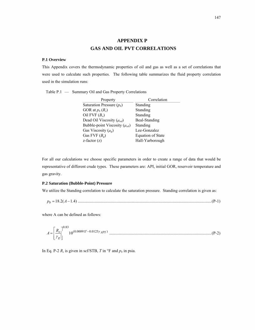
147
APPENDIX P
GAS AND OIL PVT CORRELATIONS
P.1 Overview
This Appendix covers the thermodynamic properties of oil and gas as well as a set of correlations that
were used to calculate such properties. The following table summarizes the fluid property correlation
used in the simulation runs:
Table P.1 — Summary Oil and Gas Property Correlations
Property Correlation Saturation Pressure (pb) Standing GOR at pb (Rs) Standing Oil FVF (Bo) Standing Dead Oil Viscosity (od) Beal-Standing Bubble-point Viscosity (ob) Standing Gas Viscosity (g) Lee-Gonzalez Gas FVF (Bg) Equation of State z-factor (z) Hall-Yarborough
For all our calculations we choose specific parameters in order to create a range of data that would be
representative of different crude types. These parameters are: API, initial GOR, reservoir temperature and
gas gravity.
P.2 Saturation (Bubble-Point) Pressure
We utilize the Standing correlation to calculate the saturation pressure. Standing correlation is given as:
)4.1(2.18 Apb ............................................................................................................................... (P-1)
where A can be defined as follows:
)0125.000091.0(83.0
10 APIT
g
sRA
................................................................................................. (P-2)
In Eq. P-2 Rs is given in scf/STB, T in °F and pb in psia.

148
P.3 Oil Formation Volume Factor
We also utilize the Standing Correlation to calculate the oil formation volume factor below the bubble
point pressure (Bob=f(p)). This correlation is given as:
2.15)1012(9759.0 AxBob ........................................................................................................... (P-3)
where A can be defined as follows:
TRAg
os 25.1
5.0
...................................................................................................................... (P-4)
P.4 Dead Oil Viscosity (od)
Dead oil viscosities are calculated with the Beal-Standing correlation. This correlation states that:
AT
x
APIod
200
360108.132.0
53.4
7
................................................................................................. (P-5)
where A is given as:
)]/33.8(43.0[10 APIA ...................................................................................................................... (P-6)
P.5 Saturation (Bubble-point) Viscosity
Saturated oil viscosities were calculated with the Chew and Conally correlation:
21 )( A
odob A ................................................................................................................................ (P-7)
where A1 and A2 parameters are described by Standing's best fit equation to Chew and Conally's data:
2)7102.2()4104.7(1 10 sRxsRxA
..................................................................................................... (P-8)
sRxsRxsRxA
)51074.3()3101.1()51062.8(2
10
062.0
10
25.0
10
68.0 ................................................................. (P-9)

149
P.6 Gas Viscosity (g)
The Lee-Gonzales correlation for gas viscosity is given by:
]exp[10 32
41
Agg AxA ............................................................................................................... (P-10)
where A1, A2 and A3 parameters are given as:
TM
TMA
g
g
6.192.209
)01607.0379.9( 5.1
1 ....................................................................................................... (P-11)
gMT
A 01009.04.986
448.32 .................................................................................................... (P-12)
23 2224.0447.2 AA ..................................................................................................................... (P-13)
Where Mg is defined as:
ggM 97.28 .................................................................................................................................. (P-14)
For the Lee-Gonzalez correlation we have µg in cp, g in g/cm3 and T in oR.
P.7 Gas Formation Volume Factor (Bg) and z-factor:
From the real-gas law that includes the z-factor definition, it is possible to determine that the gas
formation volume factor is given by:
p
zTBg 02827.0 .............................................................................................................................. (P-15)
with T in oR and p are given in psia.
For the z-factor, Hall and Yarborough presented an accurate representation of the Standing-Katz chart.
This calculation requires a Newton-Raphson convergence scheme to solve for the z-factor. The following
set of equations summarizes Hall and Yarborough's proposed correlation:
y
pz pr ......................................................................................................................................... (P-16)

150
])1(2.1exp[06125.0 2tt .......................................................................................................... (P-17)
and t is given by:
rTt
1 ............................................................................................................................................... (P-18)
The y-parameter (y represents the product of a van der Waals co-volume and density) can be obtained by a
Newton-Raphson calculation:
)82.218.2(32
2323
432
)4.422.2427.90(
)58.475.976.14()1(
0)(
t
pr
yttt
yttty
yyyypyf
........................................................................................................................................................... (P-19)
with df(y)/dy being:
)82.218.2(32
324
432
)4.422.2427.90()82.218.2(
)16.952.1952.29()1(
4441)(
tytttt
yttty
yyyy
dy
ydf
........................................................................................................................................................... (P-20)
References:
1. Whitson, G.H and Brule, M.R.: "Phase Behavior", SPE (2000), 18-25

151
VITA
Name: María Alejandra Nass
Address: Harold Vance Department of Petroleum Engineering
Texas A&M University
3116 TAMU - 507 Richardson Building
College Station, TX 77843
E-mail Address: [email protected]
Education: Universidad Metropolitana, Caracas, Venezuela
B.S. Chemical Engineering
October 1999
Ecole Nationale Supérieure du Pétrole et des Moteurs (ENSPM),
Rueil- Malmaison, France
M.S. Petroleum Engineering and Project Development
Diplôme d'Ingénieur
October 2001
Texas A&M University, College Station, Texas, USA
M.S. Petroleum Engineering
May 2010
Affiliations: Society of Petroleum Engineers
Related Documents