Inexpensive Fluid Flow Visualization in a Microfluidic Channel ...

Bridges: A Journal of Student Research Bridges: A Journal of Student Research

Issue 13 Article 2

2020

Inexpensive Fluid Flow Visualization in a Microfluidic Channel Inexpensive Fluid Flow Visualization in a Microfluidic Channel

Experiment Overview Experiment Overview

Maoling Chu Coastal Carolina University

Follow this and additional works at: https://digitalcommons.coastal.edu/bridges

Part of the Engineering Science and Materials Commons, and the Physics Commons

Recommended Citation Recommended Citation Chu, Maoling (2020) "Inexpensive Fluid Flow Visualization in a Microfluidic Channel Experiment Overview," Bridges: A Journal of Student Research: Vol. 13 : Iss. 13 , Article 2. Available at: https://digitalcommons.coastal.edu/bridges/vol13/iss13/2

This Article is brought to you for free and open access by the Journals and Peer-Reviewed Series at CCU Digital Commons. It has been accepted for inclusion in Bridges: A Journal of Student Research by an authorized editor of CCU Digital Commons. For more information, please contact [email protected].

Inexpensive Fluid Flow Visualization in a Microfluidic Channel Experiment Overview

Maoling ChuCoastal Carolina University

Department of Physics and Engineering Science

ABSTRACT

Flow visualization is vital to describe the motion of a fluid in microfluidic channels. This paper summarizes and lists systems based on two common visualization technique categories: particle-based techniques and scalar-based techniques. For this experiment, microfluidic chan-nels were created using PDMS (polydimethylsiloxane). Based on our results and many fab-rication trials, it was difficult to say whether this experiment was easy or inexpensive. If the first channel made by the researchers had successfully worked, it would have been clear that utilizing PDMS to fabricate a microfluidic channel for flow visualization was cheap and easy. However, no fully successful microfluidic chips were made after twenty attempted trials. Al-though, it should be stated that some of the microfluidic chip were semi-successful, meaning that the microfluidic chips worked to an extent or they worked initially before failing. Since so much PDMS was used to make the microfluidic chips, it is not necessarily inexpensive to achieve flow visualization in comparison with other experimental methods.After fabricating the channels, different mixtures were pushed through the channels to analyze the flow and visualize the velocity profile. This experiment is potentially suitable for under-graduate researchers to complete because it is safe in a laboratory. This paper also demon-strates the use of two tools, PhysMo, which is used for video analysis, and ANSYS, which is used for ideal condition analysis and complex calculations. Both scalar-based techniques and particle-based techniques were used to characterize the velocity of the laminar flow within the microchannels, the speed of which will be greatest in the center of the channel and close to zero near the walls.

Keywords: Fluid Flow Visualization, Microfluidic Channel, Inexpensive, Particle-based Techniques, Scalar-based Techniques, Reynolds Number, Navier-Stokes Equations, Poiseuille’s Law

2 MAOLING CHU

Introduction

Flow visualization, which is often used to see the flow of fluid under a microscope, is important because it allows directobservation of flow field kinematics, like the velocity profile, and other quantities that can be predicted using fluid dynamicstheory. Additionally, the experimenters can clearly explore the development of the fluid’s velocity profile through use of amicroscope (Li, 2015). Since the discovery of microfluidics and nanomicrofluidics in 1988, publications on microfluidicsand lab-on-a-chip (LOC) devices, which are miniaturized devices with channels for fluid, have evolved (Yetisen and Volpatti,2014). Analyzing flow velocity is a vital step to support and explain how the flow works in various physics and engineeringfields, such as utilizing channels to transport fuel in the aerospace engineering field (Bayt and Breuer, 2000). Nowadays,microchannels, which allow for measurements of fluidic motion, can be applied in multiple fields of science, and are espe-cially used in biomedical applications, such as to sort red blood cells from white blood cells (Li and Zhou, 2013). In addition,microchannels were one of the most important tools that allowed this experiment to work, since the small devices with printedmicrochannels can be easily fabricated by hand in a lab.

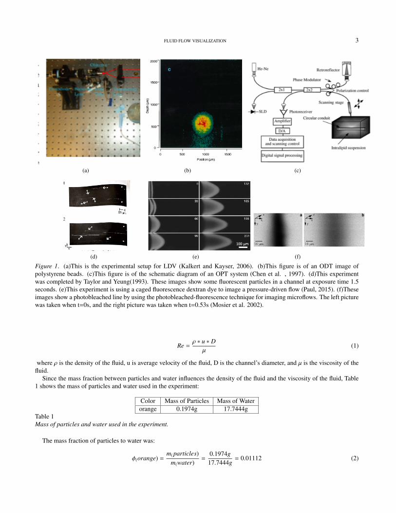
Two greatly useful ways to apply microfluidic visualization are particle-based techniques and scalar-based techniques.Particle-based techniques are used to study the motion of the bulk by following the velocity vector of particle tracers into theflow field. One particle-based technique is laser Doppler velocimetry (LDV), also named laser Doppler anemometry, whichis applied to measure the fluid velocity by making use of the principle of Doppler shift (Kayser and Kalkert, 2006)(Figure1(a)). One additional particle-based technique is optical Doppler tomography (ODT), which determines the velocity of par-ticles by resolving the speed and situation of particles in a highly scattering medium (Chen et al. 1997)(Figure 1(b and c)).Particle image velocimetry (PIV) is another particle-based technique that uses tracer particles to obtain instantaneous velocity,and then analyzes flow direction and velocity (Figure 1(d)). The micro-PIV technique is a well-developed particle-basedtechnique and is very commonly applied to analyze microfluidic visualization (Taylor and Yeung, 1993; Bayt and Breuer,2000). For scalar-based techniques, the main principle is to use molecular tracers to obtain the velocity information throughimaging two displacements of the tracers at different time intervals. There are six common ways to utilize this technique:fluorescence, caged fluorescence (Figure 1(e)), photobleaching (Figure 1(f)), phosphorescence, IR heating, and m-BLIP (mi-crobubble lensing-induced photobleaching)(Papautsky and Bhagat, 2015). There are some systems that apply scalar-basedtechniques, including scalar image velocimetry (SIV) (Dahm et al. 1992), image correlation velocimetry (ICV)(Tokumaru andDimotakis, 1995), laser-induced fluorescence (LIF)(Shehada et al. 2000), flow-tagging velocimetry (FTV)(Paul et al. 2003),and molecular-tagging velocimetry (Gendrich et al. 1996; Sinton et al. 2003).

The focus of this study was to use scalar based techniques and PIV to collect data, and then, using the Navier-Stokes equa-tions, Reynolds number, Poiseuille’s law, and calculated diameter of the particles, the data was analyzed and the fluid velocitywas determined in the micro-channels. The flow in this experiment was expected to follow Poiseuille’s law. In addition, somemicrofluidic visualization methods were reviewed. Since the small particles in the corners of the microfluidic chip were verydifficult to calculate by hand, the program ANSYS was used to calculate and check the velocity in these regions. The PhysMoprogram was also used to analyze the videos of the particles and the fluid moving through the microfluidic chip. What’s more,this experiment did not require expensive machines like a vacuum chamber for letting the bubbles evaporate out of the PDMSor a pressure pump for pumping the fluid into the microfluidic chip, as used in almost all of the systems previously mentioned.The lack of necessity for these expensive materials makes this experiment more attainable for undergraduate researchers on amore tightly controlled budget. Therefore, through this experiment, we will explore if PDMS microfluidics enable easy andinexpensive fluid flow visualization experiments.

Theory

Reynolds number

The Reynolds number is a very important factor because it is used to delineate laminar and turbulent flow conditions.When the Reynolds number is small, the influence of viscous forces on the flow field is greater than the inertial forces. Thedisturbance of the flow velocity in the flow field will be attenuated by the viscous force, and the fluid flow is stable andlaminar. On the contrary, if the Reynolds number is large, the influence of inertial forces on the flow field is greater than theinfluence of viscous forces, causing the fluid flow to be unstable. This also causes small changes in flow velocity to develop,be enhanced, and often the velocity will form a disordered and irregular turbulent flow field. For general pipelines, when theReynolds number is smaller than 2100, it is considered laminar flow. In other words, in the case of small Reynolds numbers,the relationship between force and speed of motion follows the formula of the Reynolds number:

FLUID FLOW VISUALIZATION 3

(a) (b) (c)

(d) (e) (f)

Figure 1. (a)This is the experimental setup for LDV (Kalkert and Kayser, 2006). (b)This figure is of an ODT image ofpolystyrene beads. (c)This figure is of the schematic diagram of an OPT system (Chen et al. , 1997). (d)This experimentwas completed by Taylor and Yeung(1993). These images show some fluorescent particles in a channel at exposure time 1.5seconds. (e)This experiment is using a caged fluorescence dextran dye to image a pressure-driven flow (Paul, 2015). (f)Theseimages show a photobleached line by using the photobleached-fluorescence technique for imaging microflows. The left picturewas taken when t=0s, and the right picture was taken when t=0.53s (Mosier et al. 2002).

Re =ρ ∗ u ∗ D

µ(1)

where ρ is the density of the fluid, u is average velocity of the fluid, D is the channel’s diameter, and µ is the viscosity of thefluid.

Since the mass fraction between particles and water influences the density of the fluid and the viscosity of the fluid, Table1 shows the mass of particles and water used in the experiment:

Color Mass of Particles Mass of Waterorange 0.1974g 17.7444g

Table 1Mass of particles and water used in the experiment.

The mass fraction of particles to water was:

φ(orange) =m( particles)

m(water)=

0.1974g17.7444g

= 0.01112 (2)

4 MAOLING CHU

Since the mass fraction was much smaller than 1, the mass of the particles did not alter the flow development. Additionally,the density of the microplastic particles was 1000 kg/m3. Therefore, the density of the mixture was equal to the density ofwater, which is also 1000 kg/m3. The viscosity of the water was 1 ∗ 10−3 kg/m · s because it depended on the temperature,which was 20 ◦C for this experiment (Table 2):

Density of Fluid 1E3 kg/(m)3

Viscosity 1E-3 kg/m ∗ sTable 2Density and viscosity of the fluid used in our experiment.

One goal of this experiment was to achieve laminar flow in the channels so that the flow properties were more predictable.This requires that the Reynolds number be less than 2100. We assumed that the Reynolds number was equal to 1 for simplicityin our hand calculations, and therefore, based on the formula, the velocity only depended on the various diameters of thechannels, which are shown in Table 3.

Diameter of Channel Average Velocity of Fluid1.4 mm 0.71mm/s1.05 mm 0.95mm/s

0.875 mm 1.14mm/s0.7 mm 1.43mm/s

Table 3Average velocity in various sized channels fabricated in our experiment.

Using these ideal velocities, which is assuming that there was no pressure, and comparing them with their experimentalvelocity values, which would have some pressure (equation 32, which is the average velocity through the 1.4 mm diameter),the Reynolds number is calculated to be:

Re =1E3kg/m3 ∗ 0.867mm/s ∗ 1.4mm

1E − 3kg/m · s= 1.032 ± 0.014 (3)

Therefore, it is likely that the Reynolds number is close to 1, but it is also a little bit bigger than 1 because there is somepressure on the flow that increases the velocity.

Navier-Stokes equations

The Navier-stokes equations are important for describing fluid motion. According to Newton’s second law:∑~F = m~a (4)

∑ ~F includes three different forces which are (1) pressure due to external loading, (2) gravity, and (3) adhesion due to shearforce and viscosity. Therefore, these three forces were substituted in for

∑ ~F and both sides were simplified by dividing bythe volume V: ∑ ~F

V=

m~aV

(5)

− 5 ·p + ρ~g + 5 · ¯τ = ρ~a (6)

− 5 ·p + ρ~g + 5 · ¯τ = ρ ∗ [∂~v∂t

+ (~v · 5)~v] (7)

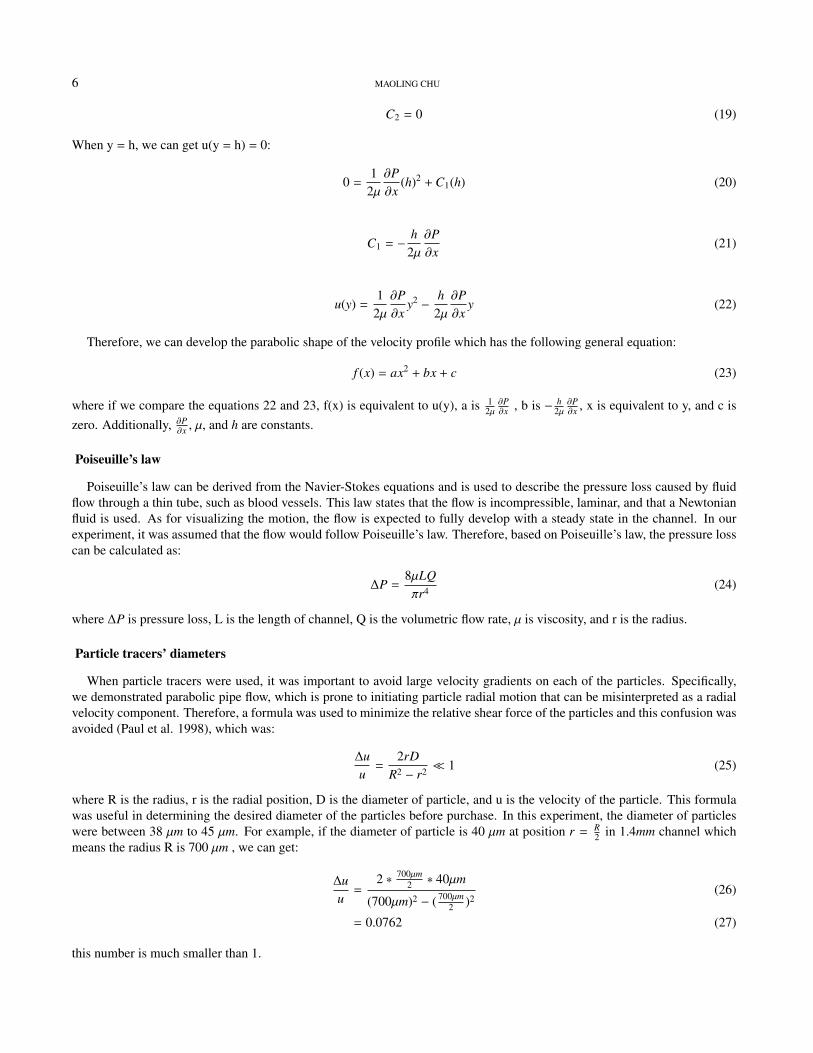
Figure 2 is a diagram of the simplistic version of a flow through one of the channels from our experiment with a fluidelement’s assigned velocity vectors and their directions. This allows us to visualize the axes that the Navier-Stokes equationswill be calculated along.

FLUID FLOW VISUALIZATION 5

Figure 2. This figure shows the axes which were drawn for visually analyzing and checking the Navier-Stokes equations.

If we assume the flow is steady, which means it will have a constant velocity, and if we assume that the x-axis and z-axisare infinite, we can develop our Navier-Stokes equations:

∂

∂t= 0 (8)

∂

∂x= 0 (9)

∂

∂z= 0 (10)

In addition, the initial velocity should be ~V = u~i, and v = w = 0. The pressure gradient should be calculated as ∂P∂x = constant

and ∂P∂z = 0 therefore:

5 · ~V =∂u∂x

+∂v∂y

+∂w∂z

(11)

Because x is infinite, and v = w = 0, we can simplify to:

5 · ~V = 0 (12)

Based on Newton’s second law, using equation 6, and doing some simplifications, we can determine on the x-axis:

0 = −∂P∂x

+ µ∂2u∂y2 (13)

and this equation can be solved by: ∫∂2u∂y2 dy =

∫1µ

∂P∂x

dy (14)

∂u∂y

=1µ

∂P∂x

y + C1 (15)∫∂u∂y

dy =

∫1u∂P∂x

y +

∫C1dy (16)

u(y) =1

2µ∂P∂x

y2 + C1y + C2 (17)

When y = 0, we can get u(y) = 0:

0 =1

2µ∂P∂x

(0)2 + C1(0) + C2 (18)

6 MAOLING CHU

C2 = 0 (19)

When y = h, we can get u(y = h) = 0:

0 =1

2µ∂P∂x

(h)2 + C1(h) (20)

C1 = −h

2µ∂P∂x

(21)

u(y) =1

2µ∂P∂x

y2 −h

2µ∂P∂x

y (22)

Therefore, we can develop the parabolic shape of the velocity profile which has the following general equation:

f (x) = ax2 + bx + c (23)

where if we compare the equations 22 and 23, f(x) is equivalent to u(y), a is 12µ

∂P∂x , b is − h

2µ∂P∂x , x is equivalent to y, and c is

zero. Additionally, ∂P∂x , µ, and h are constants.

Poiseuille’s law

Poiseuille’s law can be derived from the Navier-Stokes equations and is used to describe the pressure loss caused by fluidflow through a thin tube, such as blood vessels. This law states that the flow is incompressible, laminar, and that a Newtonianfluid is used. As for visualizing the motion, the flow is expected to fully develop with a steady state in the channel. In ourexperiment, it was assumed that the flow would follow Poiseuille’s law. Therefore, based on Poiseuille’s law, the pressure losscan be calculated as:

∆P =8µLQπr4 (24)

where ∆P is pressure loss, L is the length of channel, Q is the volumetric flow rate, µ is viscosity, and r is the radius.

Particle tracers’ diameters

When particle tracers were used, it was important to avoid large velocity gradients on each of the particles. Specifically,we demonstrated parabolic pipe flow, which is prone to initiating particle radial motion that can be misinterpreted as a radialvelocity component. Therefore, a formula was used to minimize the relative shear force of the particles and this confusion wasavoided (Paul et al. 1998), which was:

∆uu

=2rD

R2 − r2 � 1 (25)

where R is the radius, r is the radial position, D is the diameter of particle, and u is the velocity of the particle. This formulawas useful in determining the desired diameter of the particles before purchase. In this experiment, the diameter of particleswere between 38 µm to 45 µm. For example, if the diameter of particle is 40 µm at position r = R

2 in 1.4mm channel whichmeans the radius R is 700 µm , we can get:

∆uu

=2 ∗ 700µm

2 ∗ 40µm

(700µm)2 − ( 700µm2 )2

(26)

= 0.0762 (27)

this number is much smaller than 1.

FLUID FLOW VISUALIZATION 7

Methodology

Microchannel Fabrication

One of the most important steps for microfluidic visualization is to fabricate a PDMS microfludic chip. In order to create amicrofluidic channel using PDMS we followed these steps:

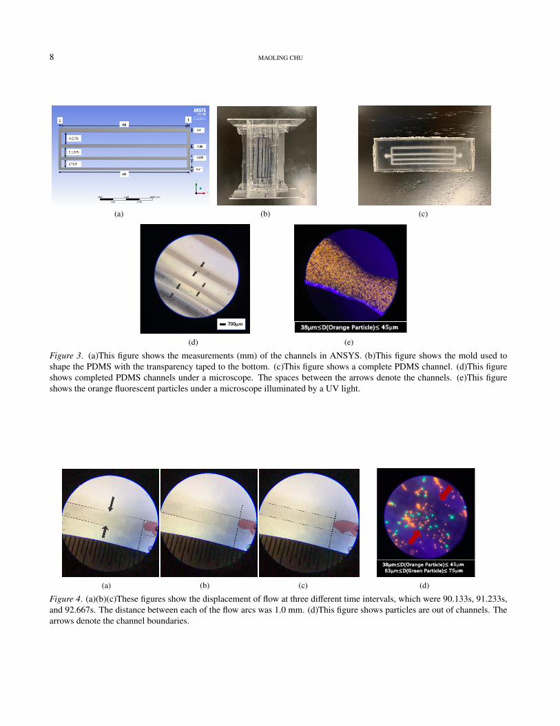
(1) Microsoft PowerPoint was utilized to design the channel pattern. The dimensions of the channel were labelled inANSYS (Figure 3(a)).

(2) This channel was printed onto transparency film using a solid-ink printer. The thickness of the ink layer determined thechannel depth in the PDMS replica.

(3) A base and curing agent were mixed at a ratio of 10:1, respectively. The mixture was then left still for 30 minutes inorder to evacuate the bubbles.

(4) The channel transparency page containing the ink was heated for 4 minutes on a hot plate at 80◦C in order to semi-meltthe ink and smooth out the channels.

(5) A rectangular shaped mold was created with an open top side for pouring in the PDMS. The transparency was pastedonto the bottom of the mold and the PDMS mixture was poured on top (Figure 3(b)). The PDMS was left for another 7 minutesto again let the bubbles evacuate the mixture. After the bubbles disappeared, the mold was placed on a hot plate at 90◦C. Themold and PDMS were left on the hot plate for 30-60 minutes, until the PDMS hardened to a solid rubbery textured device.Then the PDMS containing the channel was removed from the mold and the transparency was peeled off of the bottom.

(6) The perimeter of the PDMS was trimmed down so that the dimensions matched the size of a glass microscope slide.Holes were punched through the PDMS at both ends of the channel with a syringe tip. These holes would later become fluidinlets and outlets.

(7) A corona wand was used to treat both the PDMS and the glass microscope slide 1 cm above the surfaces for 1 minute.Then, the PDMS was flipped over onto to the glass slide and a cotton swab was used to gently press around the channels toremove the air bubbles and initiate the bond between the two surfaces.

(8) The device was heated for 30 minutes on the hot plate. After finishing this step, the PDMS channel was done (Figure3(c) and Figure 3(d)).

(9a)For the first trial, water followed by dye water was injected into the micro-channel with a syringe.(9b)For the second trial, a particle solution was mixed and injected into the micro-channel with a syringe. For the solution,

1 mL of dish detergent was blended with 100 mL of water. Then, 0.1974 g of particles and 17.7444 g of the water and soapsolution were mixed together(Figure 3(e)).

To visualize the flow, this experiment used two different fluids. One fluid was a combination of fluorescent particles andwater (Figure 3(e)), the other fluid was a combination of water followed by dyed water.

Visualization

The movement of the fluid through the channel was video recorded using a phone and was used to analyze the motion ofthe fluid by using a video analysis tool, PhysMo, which shows the time interval and displacement. These values were thenused to calculate the velocity of the flow. ANSYS was used to analyze the velocity of fluid in the corners of the model becausethe boundary conditions in the corners are too difficult to calculate by hand. ANSYS was also used to verify the other handcalculations.

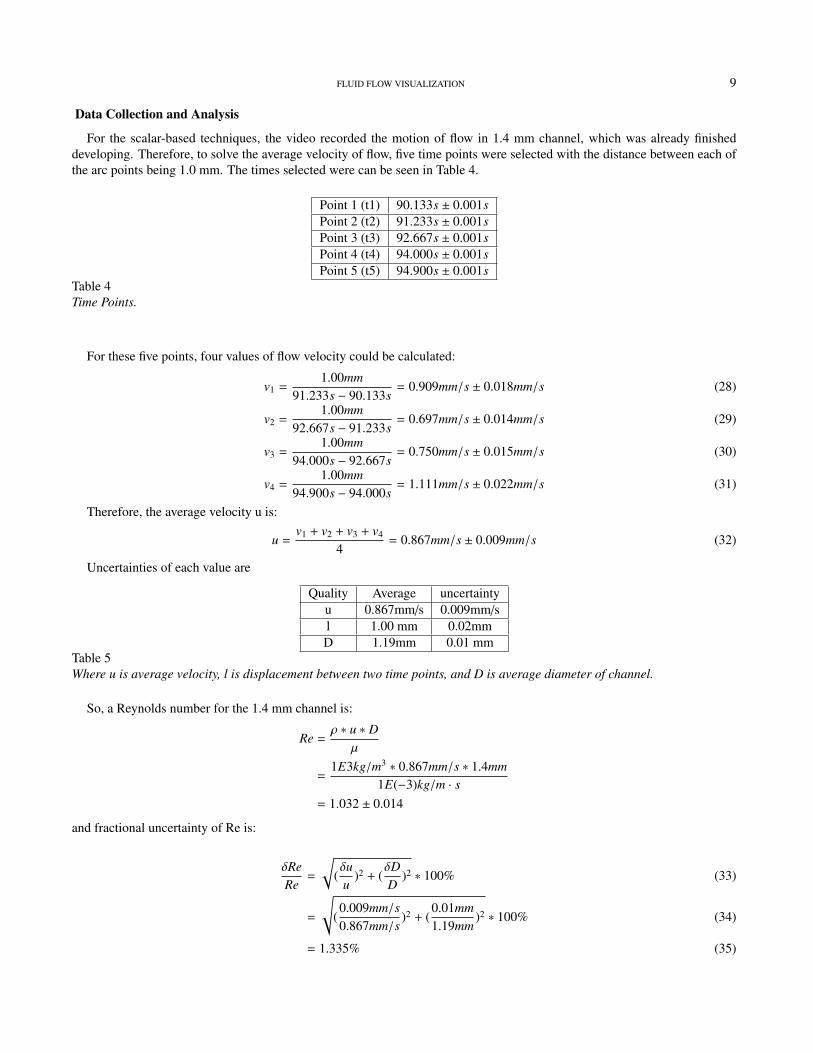
Figure 4 (a, b, and c) shows the travel of the flow as recorded by the video. In all three of these pictures, the flow hasalready moved into the fully developed region. This means that the flow will keep the same velocity throughout the rest of thechannel.

The micro-PIV system failed to measure the velocity of the particles. The microfluidic chip allowed water through thechannel initially but would not allow the particle mixture to pass through. There are two likely reasons to explain this problem.The first possible reason is that the addition of dish washing soap to the mixture, which was added to emulsify the particleswith the mixture, may have changed the density since dish washing soap has an average density of 932kg/m3. The secondpossible reason is that by first applying pressure with the syringe to force water into the channels the bond between the PDMSand the glass microscope slide was already weakened. Then, by adding more pressure to force the particle mixture into thechannels the bonds released causing leakage. Figure 4 (d) displays leakage of the particle solution out of the channels.

8 MAOLING CHU

(a) (b) (c)

(d) (e)

Figure 3. (a)This figure shows the measurements (mm) of the channels in ANSYS. (b)This figure shows the mold used toshape the PDMS with the transparency taped to the bottom. (c)This figure shows a complete PDMS channel. (d)This figureshows completed PDMS channels under a microscope. The spaces between the arrows denote the channels. (e)This figureshows the orange fluorescent particles under a microscope illuminated by a UV light.

(a) (b) (c) (d)

Figure 4. (a)(b)(c)These figures show the displacement of flow at three different time intervals, which were 90.133s, 91.233s,and 92.667s. The distance between each of the flow arcs was 1.0 mm. (d)This figure shows particles are out of channels. Thearrows denote the channel boundaries.

FLUID FLOW VISUALIZATION 9

Data Collection and Analysis

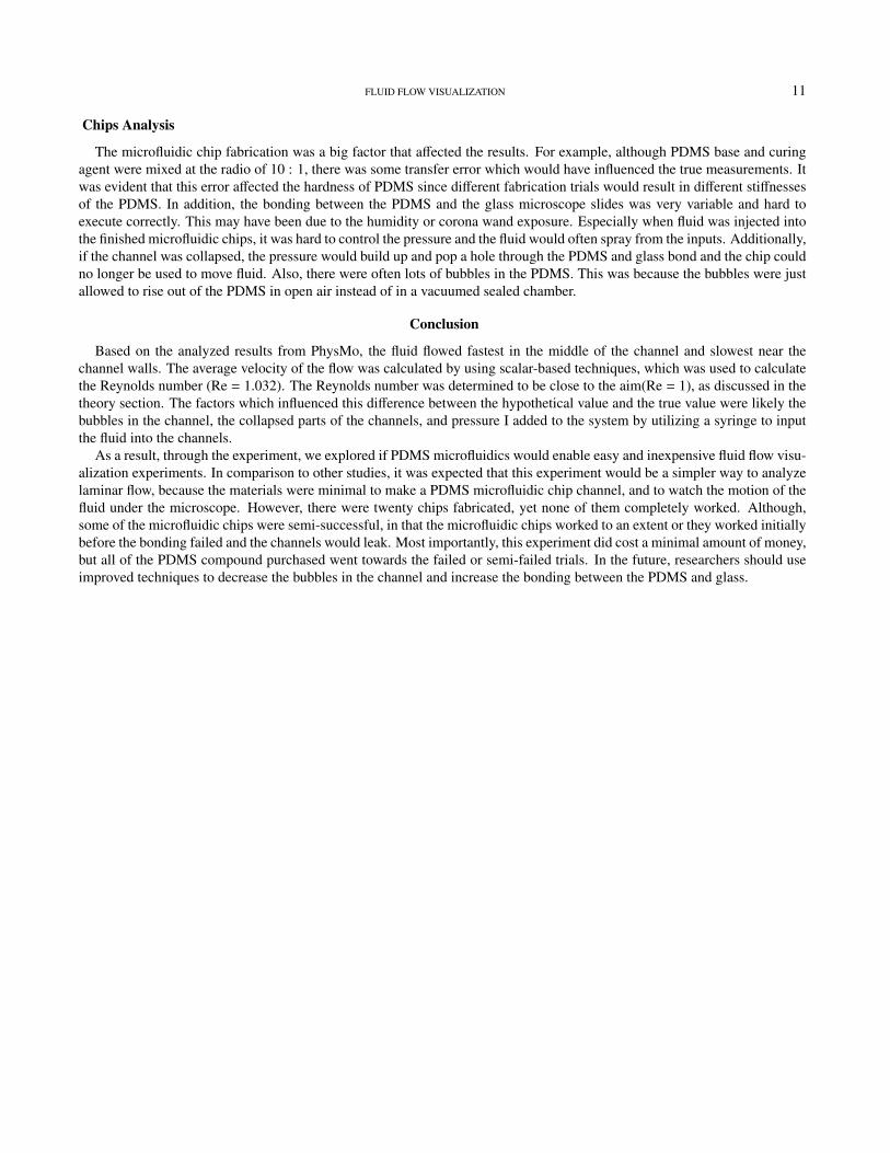
For the scalar-based techniques, the video recorded the motion of flow in 1.4 mm channel, which was already finisheddeveloping. Therefore, to solve the average velocity of flow, five time points were selected with the distance between each ofthe arc points being 1.0 mm. The times selected were can be seen in Table 4.

Point 1 (t1) 90.133s ± 0.001sPoint 2 (t2) 91.233s ± 0.001sPoint 3 (t3) 92.667s ± 0.001sPoint 4 (t4) 94.000s ± 0.001sPoint 5 (t5) 94.900s ± 0.001s

Table 4Time Points.

For these five points, four values of flow velocity could be calculated:

v1 =1.00mm

91.233s − 90.133s= 0.909mm/s ± 0.018mm/s (28)

v2 =1.00mm

92.667s − 91.233s= 0.697mm/s ± 0.014mm/s (29)

v3 =1.00mm

94.000s − 92.667s= 0.750mm/s ± 0.015mm/s (30)

v4 =1.00mm

94.900s − 94.000s= 1.111mm/s ± 0.022mm/s (31)

Therefore, the average velocity u is:

u =v1 + v2 + v3 + v4

4= 0.867mm/s ± 0.009mm/s (32)

Uncertainties of each value are

Quality Average uncertaintyu 0.867mm/s 0.009mm/sl 1.00 mm 0.02mmD 1.19mm 0.01 mm

Table 5Where u is average velocity, l is displacement between two time points, and D is average diameter of channel.

So, a Reynolds number for the 1.4 mm channel is:

Re =ρ ∗ u ∗ D

µ

=1E3kg/m3 ∗ 0.867mm/s ∗ 1.4mm

1E(−3)kg/m · s= 1.032 ± 0.014

and fractional uncertainty of Re is:

δReRe

=

√(δuu

)2 + (δDD

)2 ∗ 100% (33)

=

√(0.009mm/s0.867mm/s

)2 + (0.01mm1.19mm

)2 ∗ 100% (34)

= 1.335% (35)

10 MAOLING CHU

As a result, the Re is 1.032, and fractional uncertainty is 1.335%, which is smaller than 5%.

Result

ANSYS Example

There are two examples to analyze the velocity. One analysis shows the velocity in four different diameters of channelwhose diameters are 1.4mm, 1.05mm, 0.875mm, and 0.7mm. The initial velocity is 0.867mm/s (Figure 5 (a)).

An example simulation was created in ANSYS to show the particle tracers in one channel (Figure 5 (b, c and d)). Theheight of channel was 700 nm, the width of channel was 1.4 mm, and the length of channel was 48 mm. The initial velocitywas set as v = 0.867mm/s, Q = 8.428E − 10kg/s, and the diameter of particles was 41 µm. These values were based on theprevious calculations and the Reynolds number (Albari, 2009), which was:

Re(√

A) =ρ ∗ Q

µ ∗√

A(36)

where Q is the volumetric flow rate, ρ is density of fluid, µ is the viscosity of fluid, and the A is the cross-sectional area.

(a) (b)

(c) (d)

Figure 5. (a)This figure shows the axial velocity for the particle tracers through four different channels. Red indicates that thevelocity is the fastest and blue indicates that the velocity is equal to zero. Based on the picture, it is evident that the particlesin the center of the channel travel faster than the particles near the walls. (b)This figure shows the particles changing velocityin the channel. The velocity is increasing faster in the center. (c)This figure shows the particles velocities developing. Thevelocities of the particles were increasing at this time. (d)This figure shows the particles have finished increasing their velocity.Therefore, these particles will keep the same velocity through the rest of the channel. The maximum velocity in this figure is0.10297 m/s, the minimum is 0 m/s.

Experiment Summary

For the scalar-based techniques, the average velocity of flow was 0.867 mm/s and the Reynolds number was equal to 1.032,which were close to the calculations in the theory. For the micro-PIV system, we made 20 chips, but none of the chips allowedus to get the full results we set out to find.

FLUID FLOW VISUALIZATION 11

Chips Analysis

The microfluidic chip fabrication was a big factor that affected the results. For example, although PDMS base and curingagent were mixed at the radio of 10 : 1, there was some transfer error which would have influenced the true measurements. Itwas evident that this error affected the hardness of PDMS since different fabrication trials would result in different stiffnessesof the PDMS. In addition, the bonding between the PDMS and the glass microscope slides was very variable and hard toexecute correctly. This may have been due to the humidity or corona wand exposure. Especially when fluid was injected intothe finished microfluidic chips, it was hard to control the pressure and the fluid would often spray from the inputs. Additionally,if the channel was collapsed, the pressure would build up and pop a hole through the PDMS and glass bond and the chip couldno longer be used to move fluid. Also, there were often lots of bubbles in the PDMS. This was because the bubbles were justallowed to rise out of the PDMS in open air instead of in a vacuumed sealed chamber.

Conclusion

Based on the analyzed results from PhysMo, the fluid flowed fastest in the middle of the channel and slowest near thechannel walls. The average velocity of the flow was calculated by using scalar-based techniques, which was used to calculatethe Reynolds number (Re = 1.032). The Reynolds number was determined to be close to the aim(Re = 1), as discussed in thetheory section. The factors which influenced this difference between the hypothetical value and the true value were likely thebubbles in the channel, the collapsed parts of the channels, and pressure I added to the system by utilizing a syringe to inputthe fluid into the channels.

As a result, through the experiment, we explored if PDMS microfluidics would enable easy and inexpensive fluid flow visu-alization experiments. In comparison to other studies, it was expected that this experiment would be a simpler way to analyzelaminar flow, because the materials were minimal to make a PDMS microfluidic chip channel, and to watch the motion of thefluid under the microscope. However, there were twenty chips fabricated, yet none of them completely worked. Although,some of the microfluidic chips were semi-successful, in that the microfluidic chips worked to an extent or they worked initiallybefore the bonding failed and the channels would leak. Most importantly, this experiment did cost a minimal amount of money,but all of the PDMS compound purchased went towards the failed or semi-failed trials. In the future, researchers should useimproved techniques to decrease the bubbles in the channel and increase the bonding between the PDMS and glass.

12 MAOLING CHU

References

[1] Akbari M, Sinton D, Bahrami M. Pressure Drop in Rectangular Microchannels as Compared With Theory Based onArbitrary Cross Section. ASME. J. Fluids Eng. 2009;131(4):041202-041202-8. doi:10.1115/1.3077143.

[2] Ali K. Yetisen and Lisa R. Volpatti (2014) Patent protection and licensing in microfluidics. DOI: 10.1039/c4lc00399c

[3] Bayt RL, Breuer KS (2000) Fabrication and testing of micro-sized cold-gas thrusters in micropropulsion of small space-craft. In: Micci M, Ketsdever A (eds), Progress in Astronautics and Aeronautics, vol 187. AIAA, Reston, VA, pp381âAS398

[4] B.P. Mosier, J.I. Molho, J.G. Santiago. Photobleached-fluorescence imaging of microflows. Ex-periments in Fluids. 2002;33(4):545. Retrieved from http://search.ebscohost.com/login.aspx?direct=true&db=edo&AN=ejs3821812&site=eds-live.

[5] Christin Kalkert, and Jona Kayser (2006). Laser Doppler Velocimetry.

[6] Dahm, Werner J. A.; Su, Lester K.; Southerland, Kenneth B. (1992). "A scalar imaging velocimetry technique forfully resolved fourâARdimensional vector velocity field measurements in turbulent flows." Physics of Fluids A: FluidDynamics 4(10): 2191-2206.

[7] Flow-Tagging Velocimetry for Hypersonic Flows Using Fluorescence of Nitric Oxide Paul M. Danehy, Sean O’, Byrne,A. Frank P. Houwing, Jodie S. Fox, and Daniel R. Smith AIAA Journal 2003 41:2, 263-271

[8] Gendrich, C.P. and Koochesfahani, M.M. Experiments in Fluids (1996) 22:67. Retrieved fromhttps://doi.org/10.1007/BF01893307

[9] Li, D.(2015). Encyclopedia of microfluidics and nanofluidics. Retrieved fromhttp://search.ebscohost.com/login.aspx?direct=true&db=ca t01539a&AN=ccuc.b1901317&site=eds-live

[10] Li, X. J., and Zhou, Y. (2013). Microfluidic devices for biomedical applications. Woodhead Pub. Retrieved fromhttp://search.ebscohost.com/login.aspx?direct=true&db=ca t01539a&AN=ccuc.b2136654&site=eds-live

[11] Papautsky I., Bhagat A.A.S. (2015) Microscale Flow Visualization. In: Li D. (eds) Encyclopedia of Microfluidics andNanofluidics.

[12] Paul, P. H., Garguilo, M. G., and Rakestraw, D. J. (1998). Imaging of pressure- and electrokinetically driven flows throughopen capillaries. Analytical Chemistry, 70(13), 2459âAS2467. Retrieved from https://doi.org/10.1021/ac9709662

[13] Shehada, R.E., Marmarelis, V.Z., Mansour, H.N., and Grundfest, W.S. (2000). Laser induced fluorescence attenuationspectroscopy: detection of hypoxia. IEEE Transactions on Biomedical Engineering, 47, 301-312.

[14] Sinton, D., Erickson, D., and Li, D. (n.d.)(2003). Microbubble lensing-induced photobleaching (mu-BLIP)with application to microflow visualization. EXPERIMENTS IN FLUIDS, 35(2), 178âAS187. Retrieved fromhttps://doi.org/10.1007/s00348-003-0645-6

[15] Taylor, J. A., & Yeung, E. S. (1993). Imaging of hydrodynamic and electrokinetic flow profiles in capillaries. AnalyticalChemistry, 65(20), 2928-2932. Retrieved from https://link.springer.com/article/10.1007/s10404-004-0009-4.

[16] Tokumaru, P.T. and Dimotakis, P.E. Experiments in Fluids (1995) 19: 1. Retrieved fromhttps://doi.org/10.1007/BF00192228

[17] Z. Chen, T. Milner, D. Dave, and J. Nelson, "Optical Doppler tomographic imaging of fluid flow velocity in highlyscattering media," Opt. Lett. 22, 64-66 (1997).

Maoling Chu graduated with a B.S. in Applied Physics from Coastal Carolina University

in December 2019. During her undergraduate studies, she made the Dean’s List every

semester. At CCU, she worked as a Physics tutor, learned how to organize research

projects and collaborate with classmates, and enjoyed participating in clubs. She is

pursuing her studies at Imperial College London.