Independent Slow Feature Analysis and Nonlinear Blind ...userpage.fu-berlin.de/~tobblas/publications/blazitwis_isfa_07.pdf · Independent Slow Feature Analysis and Nonlinear Blind

The final version of this article will be published inNeural Computation, published by The MIT Press.

This version does not differ significantly from the final version.

Independent Slow Feature Analysis andNonlinear Blind Source Separation

Tobias Blaschke, Tiziano Zito and Laurenz WiskottInstitute for Theoretical Biology, Humboldt University Berlin

Invalidenstraße 43, D-10115 Berlin, Germany

{t.blaschke,t.zito,l.wiskott}@biologie.hu-berlin.de

http://itb.biologie.hu-berlin.de/˜{blaschke,zito,wiskott}

Abstract

In the linear case statistical independence is a sufficient criterion for performing blind source separa-tion. In the nonlinear case, however, it leaves an ambiguity in the solutions that has to be resolved byadditional criteria. Here we argue that temporal slowness complements statistical independence well andthat a combination of the two leads to unique solutions of the nonlinear blind source separation problem.The algorithm we present is a combination of second-order Independent Component Analysis and SlowFeature Analysis and is referred to as Independent Slow Feature Analysis. Its performance is demon-strated on nonlinearly mixed music data. We conclude that slowness is indeed a useful complement tostatistical independence but that time-delayed second-order moments are only a weak measure of statisti-cal independence.

1 IntroductionIn signal processing one often has to deal with multivariate data such as a vectorial signal x(t) = [x1(t), . . . ,xM(t)]T.To facilitate the interpretation of such a signal a useful representation of the data in terms of a linear or nonlineartransformation has to be found; prominent linear examples are Fourier transformation, Principal Component Analysis,and Fisher Discriminant Analysis. In this paper we will concentrate on Blind Source Separation (BSS), which recoverssignal components (sources) that have originally generated an observed mixture. While the linear BSS problem canbe solved by resorting to Independent Component Analysis (ICA), a method based on the assumption of mutualindependence between the mixed source signal components, this is not possible in the nonlinear case. Some algorithmshave been proposed to address this problem, and we will shortly mention them below. The objective of this paper is toshow that the nonlinear BSS problem can be solved by combining ICA and Slow Feature Analysis (SFA), a method tofind a representation where signal components are varying slowly.

After a short introduction to linear BSS and ICA in Section 2.1, we present the nonlinear BSS problem andsome of the available algorithms in Section 2.2. SFA is explained in Section 3. We introduce Independent SlowFeature Analysis (ISFA) in Section 4, a combination of second-order ICA and SFA that can perform nonlinear BSS. InSection 5 the algorithm is tested on random and surrogate correlation matrices and then applied to nonlinearly mixedaudio data. An analysis of the results reveals that nonlinear BSS can be solved by combining the objectives statisticalindependence and slowness, but that time-delayed second-order moments are not a sufficient measure of statisticalindependence in our case. We conclude with a discussion in Section 6.

2 Blind source separation and Independent Component Analysis

2.1 Linear BSS and ICALet x(t) = [x1(t), . . . ,xN(t)]T be a linear mixture of a source signal s(t) = [s1(t), . . . ,sN(t)]T and be defined by

x(t) = As(t) , (1)

1

with an invertible N ×N mixing matrix A. The goal of Blind Source Separation (BSS) is to recover the unknownsource signal s(t) from the observable x(t) without any prior information. The only assumption is that the sourcesignal components are statistically independent. Given only the observed signal x(t) we want to find a matrix R suchthat the components of

u(t) = Qy(t) = QWx(t) = Rx(t) , (2)

are mutually statistically independent. Here we have divided R into two parts. First a whitening transformationy(t) = Wx(t) with whitening matrix W is applied, resulting in uncorrelated signal components yi(t) with unit varianceand zero mean, where we have assumed x(t) and also s(t) to have zero mean. In a second step a transformationu(t) = Qy(t) with orthogonal Q [Comon, 1994] results in statistically independent components ui(t).

The method of finding a representation of the observed data such that the components are mutually statisticallyindependent is called Independent Component Analysis (ICA). It has been proven that ICA solves the linear BSSproblem, apart from the fact that the source signal components can only be recovered up to scaling and permuta-tion [Comon, 1994].

There exists a variety of algorithms performing linear ICA and therefore linear BSS. They can be divided into twoclasses [Cardoso, 2001]: (i) independence is achieved by optimizing a criterion that requires higher order statistics;(ii) the optimization criterion requires auto-correlations or non-stationarity of the source signal components. For thesecond class of BSS algorithms second-order statistics is sufficient [see e.g. Tong et al., 1991].

Here we focus on class (ii) and use a method introduced by Molgedey and Schuster [1994] based only on second-order statistics. It is based on the minimization of an objective function that can be written as

ΨτICA(Q) :=

N

∑i, j=1i6= j

(C(u)

i j (τ))2

=N

∑i, j=1i6= j

(N

∑k,l=1

QikQ jlC(y)kl (τ)

)2

(3)

operating on the already whitened signal y(t). C(u)i j (τ) is an entry of a symmetrized time delayed correlation matrix

C(u) (τ) :=12〈u(t)u(t + τ)T +u(t + τ)u(t)T〉 , (4)

C(u)i j (τ) :=

12〈ui(t)u j(t + τ)+ui(t + τ)u j(t)〉 , (5)

and C(y) (τ) is defined correspondingly. Minimization of ΨτICA can be understood intuitively as finding an orthogonal

matrix Q that diagonalizes the correlation matrix with time delay τ. Since, because of the whitening, the instanta-neous correlation matrix, which is simply the covariance matrix, is already diagonal, this results in signal componentsthat are decorrelated instantaneously and at a given time delay τ. This can be sufficient to achieve statistical inde-pendence [Tong et al., 1991]. Extending this method to several time delays is straightforward and provides greaterrobustness, see e.g. [Belouchrani et al., 1997; Ziehe and Müller, 1998] and Section 5.1.

2.2 Nonlinear BSS and ICAAn obvious extension to the linear mixing model (1) has the form

x(t) = F (s(t)) , (6)

with a nonlinear function F : RN → RM that maps N-dimensional source vectors s(t) onto M-dimensional signalvectors x(t). The components xi(t) of the observable are a nonlinear mixture of the sources and like in the linear casesource signal components si(t) are assumed to be mutually statistically independent. Extracting the source signal isonly possible if F is an invertible function on the range of s(t), which we will assume from now on.

The equivalence of BSS and ICA in the linear case does not hold in general for a nonlinear function F [Hyvärinenand Pajunen, 1999; Jutten and Karhunen, 2003]. For example, given statistically independent components u1(t) andu2(t), any nonlinear functions h1 (u1) and h2 (u2) also lead to components that are statistically independent. Also anonlinear mixture of u1(t) and u2(t) can still have statistically independent components [Jutten and Karhunen, 2003].Thus in the nonlinear BSS problem independence is not sufficient to recover the original source signal and additionalassumptions about the mapping F or the source signal are needed to sufficiently constrain the optimization problem.We list some of the known methods:

• Constraints on the mapping F :

2

– F is a smooth mapping [Hyvärinen and Pajunen, 1999; Almeida, 2004];

– F is a post nonlinear (PNL) mapping [Taleb and Jutten, 1997; Yang et al., 1998; Taleb and Jutten, 1999;Taleb, 2002; Ziehe et al., 2003].

• Prior information about the source signal components:

– source signal components are bounded [Babaie-Zadeh et al., 2002];

– source signal components have time-delayed auto-correlations (referred to as temporal correlations) [Hos-seini and Jutten, 2003];

– source signal components are those that exhibit a characteristic time structure (power spectra are pairwisedifferent) [Harmeling et al., 2003].

2.3 A new approachIn our approach we do not make any specific assumption about the mapping F , although the function space availablefor unmixing will be finite-dimensional in the algorithm, which imposes some limitations on F . Since we employan ICA method based on time-delayed cross-correlations we make the implicit assumption that the sources havesignificantly different temporal structure (power spectra are pairwise different) [cf. Harmeling et al., 2003]. We alsoassume that the sampling rate is high enough, so that the input signal can be treated as if it were continuous and thetime derivative is well approximated by the difference of two successive time points.

We have seen above, that in the nonlinear case statistical independence alone is not a sufficient criterion for blindsource separation. There are infinitely many nonlinearly distorted versions of one source that are all statistically inde-pendent of another source. We propose slowness as a means to resolve this ambiguity and select a good representativefrom all the different versions of a source, because nonlinearly distorted versions of a source are usually varying morequickly than the source itself. Consider for example a sinusoidal signal component xi(t) = sin(t) and a second com-ponent that is the square of the first x j(t) = xi(t)2 = 0.5(1− cos(2t)). The second component is more quickly varyingdue to the frequency doubling induced by the squaring. We believe this argument can be made more formal and itcan be proven that, given the set of a one-dimensional signal and all its nonlinearly and continuously transformed ver-sions, the slowest signal of the set is either the signal itself or an invertibly transformed version of it [Zito and Wiskott,in preparation]. Considering this we propose, in order to perform nonlinear BSS, to complement the independenceobjective of pure ICA with a slowness objective. In the next section we will give a short introduction to Slow FeatureAnalysis, an algorithm built on the basis of this slowness objective.

3 Slow Feature AnalysisSlow Feature Analysis (SFA) is a method that extracts slowly varying signals from a given observed signal [Wiskottand Sejnowski, 2002]. This section gives a short description of the method as well as a link between SFA and second-order ICA [Blaschke et al., 2006], which provides the means to find a simple objective function for our nonlinear BSSmethod.

Consider a vectorial input signal x(t) = [x1(t), . . . ,xM(t)]T. The objective of SFA is to find a nonlinear input-outputfunction g(x) = [g1(x), . . . , gL(x)]T such that the components of u(t) = g(x(t)) are varying as slowly as possible. Asa measure of slowness we use the variance of the first derivative, so that a slow signal has on average a small slope.The optimization problem then is as follows: Minimize the objective function

∆(ui) := 〈u2i (t)〉 (7)

successively for each ui(t) under the constraints

〈ui(t)〉 = 0 (zero mean), (8)

〈(ui(t))2〉 = 1 (unit variance), (9)

〈ui(t)u j(t)〉 = 0 ∀ j < i (decorrelation and order), (10)

where 〈· 〉 denotes averaging over time. Constraints (8) and (9) ensure that the solution will not be the trivial solutionui(t) = const. Constraint (10) provides uncorrelated output signal components and thus guarantees that differentcomponents carry different information.

3

To make the optimization problem easier to solve we consider the components gi of the input-output function to bea linear combination of a finite set of nonlinear functions. We can then split the optimization procedure into two parts:(i) nonlinear expansion of the input signal x(t) into a high-dimensional feature space, and (ii) solving the optimizationproblem in this feature space linearly.

3.1 Nonlinear expansionA common method to make nonlinear problems solvable in a linear fashion is nonlinear expansion. The observedsignal components xi(t) are mapped into a high-dimensional feature-space according to

z(t) = h(x(t)). (11)

The dimension L of z(t) is typically much larger than that of the original signal. For instance, if we want to expandinto the space of second degree polynomials, we can apply the mapping

h(x) = [x1, . . . , xM, x1x1, x1x2, . . . , xMxM]T−hT0 . (12)

The dimensionality of this feature space is L = M + M (M +1)/2. The constant vector hT0 is needed to make the

expanded signal mean free.

3.2 Solution of the linear optimization problemGiven the nonlinear expansion, the nonlinear input-output function g(x) can be written as

g(x) = Rh(x) = Rz , (13)

where R is an L×L matrix which is subject to optimization. To simplify the optimization procedure we (i) choosethe nonlinearities h(·) such that z(t) is mean free and (ii) first find a transformation y(t) = Wz(t) to obtain mutuallydecorrelated components yi(t) with zero mean. Matrix W is a whitening matrix as in normal ICA:

u(t) = Qy(t) = QWz(t) = Rz(t) = g(x(t)) , (14)

where y(t) is the nonlinearly expanded and whitened signal. It can be shown [Wiskott and Sejnowski, 2002] that theconstraints (8), (9), and (10) are fulfilled trivially if the transformation Q, subject to learning, is an orthogonal matrix.To solve the optimization problem we rewrite the slowness objective (7)

∆(ui) = 〈(u1(t))2〉= qT

i 〈y(t) y(t)T〉qi =: qTi Eqi , (15)

where qi = [Qi1,Qi2, . . . ,QiL]T is the i-th row of Q and E is the matrix 〈y(t)y(t)T〉. For this optimization problemthere exists a unique solution. For i = 1 the optimal weight vector is the normalized eigenvector that correspondsto the smallest eigenvalue of E. The eigenvectors of the next higher eigenvalues produce the next slow componentsu2(t), u3(t), . . . and so forth. Typically only the first several of all L possible output components are of interest andselected.

Finding the eigenvectors is equivalent to finding the transformation Q such that QTEQ is diagonal. As describedin detail in [Blaschke et al., 2006], this leads to an objective function for SFA subject to maximization

ΨτSFA(Q) :=

L

∑i=1

(C(u)

ii (τ))2

=L

∑i=1

(L

∑k,l=1

QikQilC(y)kl (τ)

)2

, (16)

where τ is a time delay that arises from an approximation of the time derivative. We set τ = 1 because we make theapproximation y(t)≈ y(t +1)−y(t).

To understand (16) intuitively we note that slowly varying signal components are easier to predict and shouldtherefore have strong correlations in time. Thus, maximizing the time delayed auto-correlation produces a slowlyvarying signal component. Since the trace of C(y) (τ) is preserved under a rotation Q, maximizing the sum over thesquared auto-correlations tends to produce a set of most slowly varying signal components at the expense of the othercomponents, which become most quickly varying and are usually discarded.

Note the formal similarity between (3) and (16).

4

4 Independent Slow Feature AnalysisThe nonlinear BSS method proposed in this section combines the principle of independence known from linear second-order BSS methods with the principle of slowness as described above. Because of the combination of ICA and SFAwe refer to this method as Independent Slow Feature Analysis (ISFA). As already explained, second-order ICA tendsto make the output components independent and SFA tends to make them slow. Since we are dealing with a nonlinearmixture we first compute a nonlinearly expanded signal z(t) = h(x(t)) with h : RM → RL being some nonlinearfunction chosen such that z(t) has zero mean. In a second step z(t) is whitened to obtain y(t) = Wz(t). Finally weapply linear ICA combined with linear SFA on y(t) in order to find the output signal u(t), the R first component ofwhich are the estimated source signals, where R is usually much smaller than L, the dimension of the expanded signal.Because of the whitening we know that ISFA, like ICA and SFA, is solved by finding an orthogonal L×L matrix Q.We write the output signal u(t) as

u(t) = Qy(t) = QWz(t) = QWh(x(t)) , (17)

While the u1(t), . . . ,uR(t) are statistically independent and slowly varying, the components uR+1(t), . . . ,uL(t) are morequickly varying and may be statistically dependent on each other as well as on the estimated sources. The last L−Rcomponents of the output signal u(t) are irrelevant for the final result but important during the optimization procedure,see below.

To summarize, we have an M-dimensional input x(t), an L-dimensional nonlinearly expanded and whitened y(t),and an L-dimensional output signal u(t). ISFA finds an orthogonal matrix Q such that the R first components of theoutput signal u(t) are mutually independent and slowly varying. These are the estimated sources.

4.1 Objective functionTo recover R source signal components ui(t), i = 1, . . . ,R from an L-dimensional expanded and whitened signal y(t)the objective for ISFA with one single time delay τ reads

ΨτISFA(u1, . . . ,uR) := bICAΨ

τICA(u1, . . . ,uR)−bSFAΨ

τSFA(u1, . . . ,uR)

= bICA

R

∑i, j=1,i 6= j

(C(u)

i j (τ))2−bSFA

R

∑i=1

(C(u)

ii (τ))2

, (18)

where we simply combine the ICA objective (3) and SFA objective (16) for the first R components weighted by thefactors bICA and bSFA, respectively. Note that the ICA and the SFA objective are usually applied to all componentsand that in the linear case (and for one time delay τ = 1) they are equivalent Blaschke et al. [2006]. Here, they areapplied to an R-dimensional subspace in the L-dimensional expanded space, which makes them different from eachother. Ψτ

ISFA is to be minimized, which is the reason why the SFA part has a negative sign.In the linear case it is standard practice to use multiple time delays to stabilize the ICA solution, see for example

the kTDSEP algorithm by Harmeling et al. [2003]. We will see in Sections 5.1 and 5.2 that in our case multipletime-delays are actually essential to get meaningful solutions. The general expression for the objective of ISFA thenreads

ΨISFA(u1, . . . ,uR) := bICA ∑τ∈TICA

κτICAΨ

τICA−bSFA ∑

τ∈TSFA

κτSFAΨ

τSFA

= bICA ∑τ∈TICA

κτICA

R

∑i, j=1,i 6= j

(C(u)

i j (τ))2

−bSFA ∑τ∈TSFA

κτSFA

R

∑i=1

(C(u)

ii (τ))2

, (19)

where TICA and TSFA are the sets of time delays for the ICA and SFA objectives respectively, whereas κτICA and κτ

SFAare weighting factors for the corresponding correlation matrices. For simplicity we will first continue the descriptionwith only one time delay based on (18) and only later provide the full formulation with multiple time delays basedon (19).

5

4.2 Optimization procedureFrom (17) we know that C(u) (τ) in (18) depends on the orthogonal matrix Q. There are several ways to find theorthogonal matrix that minimizes the objective function. Here we apply successive Givens rotations to obtain Q. AGivens rotation is a rotation around the origin within the plane of two selected components µ and ν and has the matrixform

Qµν

i j :=

cos(φ) for (i, j) ∈ {(µ,µ) ,(ν,ν)}

−sin(φ) for (i, j) ∈ {(µ,ν)}sin(φ) for (i, j) ∈ {(ν,µ)}

δi j otherwise

(20)

with Kronecker symbol δi j and rotation angle φ. Any orthogonal L×L matrix such as Q can be written as a product ofL(L−1)/2 (or more) Givens rotation matrices Qµν (for the rotation part) and a diagonal matrix with diagonal elements±1 (for the reflection part). Since reflections do not matter in our case we only consider the Givens rotations as isoften done in second-order ICA algorithms [e.g. Cardoso and Souloumiac, 1996] (but note that here it is applied to asubspace). The objective (18) as a function of a Givens rotation Qµν reads

Ψτ,µν

ISFA (Qµν) = bICA

R

∑i, j=1i6= j

(L

∑k,l=1

Qµν

ik Qµν

jl C(u′)kl (τ)

)2

−bSFA

R

∑i=1

(L

∑k,l=1

Qµν

ik Qµν

il C(u′)kl (τ)

)2

, (21)

where u′ is some intermediate signal during the optimization procedure. For each Givens rotation there exists an angleφmin with minimal Ψ

τ,µν

ISFA. Successive application of Givens rotations Qµν with the corresponding rotation angle φminleads to the final rotation matrix Q yielding

C(u) (τ) = QTC(y) (τ)Q . (22)

In the ideal case the upper left R×R submatrix of C(u) (τ) is diagonal with a large trace ∑Ri=1 C(u)

ii (τ).

Applying a Givens rotation Qµν in the µν-plane changes all auto- and cross-correlations C(u′)i j (τ) with at least one

of the indices equal to µ or ν. There exist two invariances under such a transformation, which can be described as(C

(u′)µi (τ)

)2

+(

C(u′)νi (τ)

)2

= const ∀i 6∈ {µ,ν}, (23)(C

(u′)µµ (τ)

)2

+(

C(u′)µν (τ)

)2

+(

C(u′)νµ (τ)

)2

+(

C(u′)νν (τ)

)2

= const. (24)

Assume we want to minimize ΨτISFA for a given R, where R denotes the number of signal components we want to

extract. Applying a Givens rotation Qµν we have to distinguish three cases

• Case 1 Both axes, µ and ν, lie inside the subspace spanned by the first R axes (µ,ν ≤ R) (see Fig. 1a):The sum over all squared cross correlations of all signal components that lie outside the R-dimensional subspaceis constant as well as that of all signal components inside the subspace. The former holds because of the firstinvariance (23) and the latter because of the first (23) and second invariance (24). There is no interaction betweeninside and outside, in fact the objective function is exactly the objective for an ICA algorithm based on second-order statistics, e.g. TDSEP or SOBI [Ziehe and Müller, 1998; Belouchrani et al., 1997]. In [Blaschke et al.,2006] it has been shown that this is equivalent to SFA in the case of a single time delay of τ = 1.

• Case 2 Only one axis, w.l.o.g. µ, lies inside the subspace; the other, ν, lies outside (µ ≤ R < ν) (see Fig. 1b):Since one axis of the rotation plane lies outside the subspace, u′µ in the objective function can be optimized atthe expense of the u′ν outside the subspace. A rotation of π/2, for example, would simply exchange components

u′µ and u′ν. For instance, according to (23)(

C(u′)µi

)2

can be optimized at the expense of(

C(u′)νi

)2

with i ∈

{1, . . . ,R}; according to (24)(

C(u′)µµ

)2

can be optimized at the expense of(

C(u′)µν

)2

,(

C(u′)νµ

)2

, and(

C(u′)νν

)2

.

This gives the possibility to find the slowest and most independent components in the whole space spanned byall L axes in contrast to Case 1 where the minimum is searched within the subspace spanned by the first R axesconsidered in the objective function.

6

µ ν R L

µ

ν

R

L

u´u´u´

u´

u´ u´ u´ u´

(a) Case 1

µ

R

ν

L

µ R ν L

u´u´

u´u´

u´ u´ u´ u´

(b) Case 2

ν

L

R

µ ν

µ

L

u´

u´

u´u´

u´ u´Ru´ u´

(c) Case 3

Figure 1: Each square represents a squared cross or auto-correlation(

C(u′)i j

)2

where index i( j) denotes the row

(column) of the square. Dark squares indicate all entries that are changed by a rotation in the µ-ν-plane. L is thedimensionality of the expanded signal u′ and R the number of signal components u′i(t) subject to optimization.The entries incorporated in the objective function are located in the upper left corner as indicated by the dashedline.

7

• Case 3 Both axes lie outside the subspace (R < µ,ν) (see Fig. 1c):A Givens rotation with the two rotation axes outside the relevant subspace does not affect the objective functionand can therefore be disregarded.

To optimize the objective function of ISFA (18) we need to calculate the explicit form of the objective function Ψτ,µν

ISFAin (21). By inserting the Givens rotation matrix (20) into the objective function (21), and considering the case withmultiple time delays, we can write the objective as a function of the rotation angle φ

Ψµν

ISFA (φ) = bICA

(ec +

2

∑β=0

eβ cos4−β(φ)sinβ(φ)

)

−bSFA

(dc +

4

∑α=0

dα cos4−α(φ)sinα(φ)

)(25)

with constants e and d that depend only on the C(u′)kl before rotation. Further simplification [cf. Blaschke and Wiskott,

2004] leads to

Case 1: Ψµν

ISFA (φ) = A0 +A4 cos(4φ+φ4) (26)Case 2: Ψ

µν

ISFA (φ) = A0 +A2 cos(2φ+φ2)+A4 cos(4φ+φ4) (27)

with a single minimum (if w.l.o.g. φ ∈[−π

2 , π

2

]), which can be calculated easily. The derivation of (26) and (27)

involves various trigonometric identities and, because of its length, is documented in the appendix.The iterative optimization procedure with successive Givens rotations can now be described as follows:

1. Initialize Q′ = I and compute C(u′) (τ) = C(y) (τ)∀τ ∈ TICA∪TSFA with (4) and Ψ′ISFA with (19).

2. Choose a random permutation of the set of axis pairs:P = σ

({(µ,ν), with µ ≤ R and µ < ν ≤ L

}).

3. Go systematically through all axis pairs in P. For each axis pair:

(a) determine the optimal rotation angle φµν

min for the selected axes with (26) or (27),

(b) compute the Givens rotation matrix Qµν(φ

µν

min

)defined by (20),

(c) update C(u′) (τ) using C(u′) (τ)→ (Qµν)T C(u′) (τ)Qµν,

(d) update Q′ according to Q′ → QµνQ′,

(e) backup the previous objective-function value Ψ′′ISFA = Ψ′

ISFA,

(f) calculate the new objective-function value Ψ′ISFA with (19) using the updated C(u′) (τ) from (3c),

(g) store the relative decrease of the objective function valueΨ′′

ISFA−Ψ′ISFA

|Ψ′′ISFA|

.

4. Go to 2 until the relative decrease of the objective function is smaller than ε � 1 for all axis pairs in P.

5. Set Q = Q′ and u(t) = Qy(t).

In Step 2 it is important to note that the rotation planes of the Givens rotations are selected from the whole L-dimensional space (although we avoid the irrelevant Case 3 by requiring µ ≤ R, see Fig. 1) whereas the objectivefunction only uses information of correlations among the first R signal components u′i. Since Qµν is very sparse, theGivens rotation in Step 3c does not require a full matrix-multiplication but can be computed more efficiently. Notethat the algorithm works on the intermediate correlation matrices C(u′) (τ) and not on the signals themselves; the inputsignal y(t) is used only in the initialization (Step 1) and at the end (Step 5) when the output signal u(t) is computed.To circumvent the problem of getting stuck in local optima of the objective function, a random rotation of the outerspace (ν > µ > R) can be performed after convergence in Step 4, and the algorithm can be restarted at Step 2.

8

5 ResultsTo evaluate the performance of ISFA we tested the algorithm first on random matrices to check how many matricesare needed to get meaningful results, then on surrogate matrices to check that the algorithm reliably converges to theglobal optimum under these ideal conditions, and then on a difficult although low-dimensional mixture of audio datato show how it performs on real data. In order to reduce the problem of local optima, we use SFA as a preprocessingstep. That choice follows from the empirical observation that SFA is always able to extract the first source signal. Tostabilize the ISFA solutions even further we typically run the optimization routine once with the first axis fixed, andthen once more following the procedure described in Section 4.2. Throughout the paper the SFA time-delay set andthe weighting factors were as follows:

TSFA ={

1}

(28)κ

τSFA = 1 for τ = 1 (29)

κτICA = 1 ∀τ ∈ TICA ; (30)

This particular choice makes it easy to interpret the ISFA objective function (19): The SFA part is the plain SFAobjective function of (16); the ICA part is the plain ICA objective function of (3) extended to several time delays. Ifwe would choose more than one time delay for the SFA part, the interpretation in terms of slowness would becomeless clear [see Blaschke et al., 2006]. TICA depends on the experiment, see below.

5.1 Tests with random matricesFirst consider only the ICA part of the objective function (19). Its purpose is to guarantee statistical independenceof the estimated sources by simultaneously diagonalizing the R×R upper left submatrix of T time-delayed L× Lcorrelation matrices, where T is the number of elements in TICA. However, for the ICA term to be useful we have totake sufficiently many matrices into account so that simultaneous submatrix-diagonalization is not trivial. For instance,a single symmetric matrix can always be fully diagonalized by the orthonormal set of its eigenvectors. Thus for R = Land T = 1 one has to take at least two matrices to avoid this spurious solution, which would be found even if there areno underlying statistically independent sources.

To estimate the minimum number of matrices needed, we ran ISFA with bSFA = 0 on randomly generated sym-metric matrices Aτ, τ = 1, ...,T , for different values of L, R, and T . The subdiagonalization was considered suc-cessful if E :=

√〈A2

i j〉τ, j,i> j, i.e. the square root of the averaged squared non-diagonal terms, was below a threshold

Ecrit := 10−3. For fixed L and R < L we typically observe that a high degree of subdiagonalization is possible forT = 2. For T > 2 the subdiagonalization is still possible but at a lower degree with increasing T , until a critical Tcrit isreached, for which the degree of subdiagonalization displays a sharp transition where E crosses the threshold Ecrit andremains stable after that.

The estimated critical number of time delays Tcrit for L ∈ {9,20} and different values of R are given in Table 1. Inthe simulations that follow, we have M = R = 2 and use ISFA3 and ISFA5 (ISFAn refers to ISFA with polynomials ofdegree n) resulting in L = 9 and L = 20, respectively. From the table we see that with T = 50 we are well above Tcritin both cases.

R 2 3 4 5 6 7 8 9 10 >10L = 9 Tcrit 18 8 5 4 3 2 2 2 - -L = 20 Tcrit 36 19 13 9 7 6 5 4 3 2

Table 1: Critical number of time delays, Tcrit, for different values of L and R.

5.2 Tests with surrogate matricesTo test the performance of ISFA (now including the SFA part) in absence of noise, finite-size effects, or any other kindof perturbation we carried out an experiment with T > 1 surrogate matrices, prepared such that they have a uniqueexact solution (except for permutations). The first matrix, with τ = 1, is fully diagonal with the diagonal elementsordered by decreasing absolute value, with the exception of the second and last element, which are swapped. Allother T −1 matrices are random symmetric matrices with a diagonal (R+RICA)× (R+RICA) upper submatrix. SFAalone only sees the first matrix (cf. 28, 29) and would favor a solution in which the last component is swapped back

9

into the R×R subspace in place of the small second component. ICA alone would favor any permutation of thefirst (R + RICA) components equally well, because for any of these permutations the R×R upper submatrices are alldiagonal. In this example ICA should prevent SFA from swapping the last component into the R×R subspace andSFA should disambiguate the many equally valid ICA solutions by selecting the largest diagonal elements, i.e. theslowest components, in the first matrix.

This set of matrices constitutes a fixed point for the ISFA algorithm. If we run ISFA directly on these matriceswe get Q = I. If we now apply a random rotation matrix Qrand to the set of matrices, we would expect ISFA to finda matrix Q that inverts this rotation and returns the R original first components, but in any arbitrary order. Thus, theR×R submatrix of the product P := QQrand should be a permutation matrix for perfect unmixing.

We performed 10,000 independent tests with R = 2, RICA = 2, L = 9, and T = 50, somewhat imitating the case oftwo nonlinearly mixed independent sources and an expansion space of all polynomials of degree three. The estimatedcritical number of matrices Tcrit is 18. Using 50 matrices we rule out any spurious solution as discussed in Section 5.1.As a measure of performance we used the reconstruction error measure first introduced by Amari et al. [1995] in theformulation given in [Blaschke and Wiskott, 2004]:

E =1

R2

(R

∑i=1

(R

∑j=1

|Pi j|maxk |Pik|

−1

)+

R

∑j=1

(R

∑i=1

|Pi j|maxk |Pk j|

−1

)). (31)

An experiment is considered to be successful if the unmixing error is smaller than 10−5. We found that ISFA alwaysrecovered the original components and that this 100% success rate was largely independent of the scaling factors bICAand bSFA, which we therefore set to bICA = bSFA = 1 for this experiment.

5.3 Tests with twisted audio dataIn the third experiment we tested the algorithm on 171 pairs of 19 nonlinearly mixed music excerpts. The samplevalues of the 19 excerpts were in the range of [−1,+1); the mean had an average value of (−10± 110)× 10−6

(mean ± std); the standard deviation had an average value of 0.16±0.07, its minimum and maximum value was 0.02and 0.27, respectively. One additional music excerpt was discarded, because it had extreme peaks, which led to astrong nonlinear distortion due to the SFA part and low correlations with the source even though it was in principleextracted correctly. All audio signals were 221 = 2,097,152 samples long and had a CD-quality sampling frequencyof 44,100 Hz. We used the nonlinear mixture introduced by Harmeling et al. [2003] defined by

x1(t) = (s2(t)+3s1(t)+6)cos(1.5πs1(t)) , (32)x2(t) = (s2(t)+3s1(t)+6)sin(1.5πs1(t)) . (33)

This is quite an extreme nonlinearity and the unmixing performance depends strongly on the standard deviation ofthe sources. For the ICA part of the objective in (19) we used 50 time delays evenly spaced within 1 and 44,100,corresponding to a time scale up to 1 second. The number of time delays is greater than the critical number Tcrit,which is 18 for an expansion with polynomials of degree three, and 36 for polynomials of degree five. In orderto evaluate the performance of the algorithm fairly we used linear regression to check if the nonlinear mixture wasindeed invertible within the available space. Two orthogonal directions were fit within the whitened expanded spaceto maximize the correlation with the original sources. Within the space of polynomials of degree three, there were anumber of cases (51 examples, 30% of the total) where the two sources were not found by linear regression, whichmeans the nonlinear mixture was not invertible within the available expanded space. This is the main reason forfailures in ISFA3. Within the space of polynomials of degree five the mixture was always invertible. The scalingfactor bSFA was kept constant and equal to 1, while bICA was manually tuned for each example in order to maximizethe correlation between estimated and original sources. For polynomials of degree three we tested different values ofbICA equidistant on a logarithmic scale between 0 and 10000. The number of tested values varied between 5 and 40depending on how clear and robust the optimum was. For polynomials of degree one and five we largely adopted thevalues found for polynomials of degree three; only if the algorithm failed with these values did we retune bICA with 20equidistant values. This tuning resulted in values between 0 and 1000. A source signal is considered to be recoveredif the correlation with the estimated source is greater than 0.9.

Scatter plots of a successful example are shown in Figure 2 and a summary of the results is given in Table 2. ISFAis able to separate the nonlinearly mixed sources in about 70% of the cases in which unmixing was possible at all.This is remarkable given the extreme nonlinearity of the mixture and a chance level of unmixing of less than 0.01%,as we have tested by numerical simulations. However, there remains a failure rate of about 30%, which is puzzlinggiven the perfect performance on the surrogate matrices (Sec. 5.2). We investigate this in the next section.

10

(a) (b) (c)

(d) (e)

Figure 2: Scatter plot of two sources, their nonlinear mixture, and the estimated sources. (a) Sources, (b) mixture, (c)sources estimated by ISFA5, (d) first source vs. estimated first source, (e) second source vs. estimated second source.Correlation coefficients of estimated sources and original sources were 0.996 and 0.998.

# rec. src. REG1 REG3 REG5

2 5% (8) 70% (120) 100% (171)1 54% (93) 30% (51) 0% (0)0 41% (70) 0% (0) 0% (0)

# rec. src. ISFA1 ISFA3 ISFA5

2 5% (8) 50% (85) 71% (122)1 50% (85) 34% (59) 18% (30)0 45% (78) 16% (27) 11% (19)

% correct 100%( 8

8

)71%

( 85120

)71%

( 122171

)Table 2: The upper part shows percentages of cases where both, one, or none of the two sources were recovered bylinear regression (supervised) in the original space (REG1) or in the expanded space with polynomials of degree three(REG3) or five (REG5). The lower part shows the same for ISFA (unsupervised except for the tuning of bICA). Eachentry indicates the percentage (and number) of pairs with respect to the total of 171 pairs. The last line presents thepercentage of both sources recovered correctly with respect to the number of mixtures invertible within the availableexpanded space by linear regression. Note that in the case of two recovered sources chance level is always smallerthan 0.01%.

11

5.4 Analysis of failure casesWhy did ISFA fail in about 30% of the cases where a good solution was available by linear regression? The values ofthe objective function ΨISFA (19) and its two parts ΨICA and ΨSFA give us some information about possible reasons.Consider the following four different cases:

1. In 1 out of the 35 true failures for ISFA3 and never for ISFA5 it is the case that ΨISFA of the sources estimated byISFA is greater than the ΨISFA of the sources estimated by linear regression. In this case the algorithm obviouslygot stuck in a local optimum.

2. In 15 and 26 out of the 35 and 49 true failures for ISFA3 and ISFA5, respectively, ΨISFA of the sources estimatedby ISFA is smaller than the ΨISFA of the sources estimated by linear regression, but either ΨICA or ΨSFA is greaterthan the corresponding linear-regression value. This indicates that the tuning of the weighting factors bSFA andbICA might not have been fine enough. However, it could also be that there is an abrupt transition betweensolutions where ΨICA is greater to solutions where ΨSFA is greater than the corresponding linear-regressionvalue.

3. In 6 and 3 out of the 35 and 49 true failures for ISFA3 and ISFA5, respectively, ΨICA and ΨSFA of the sourcesestimated by ISFA are both smaller than the ones of the linear-regression estimate and greater than the ones ofthe original sources. Neither a local optimum nor the weighting factors are a plausible cause for the failure inthese cases. It might be that the expansion was too low-dimensional and that a higher-dimensional expansionwould have yielded the correct solution.

4. In 13 and 20 out of the 35 and 49 true failures for ISFA3 and ISFA5, respectively, ΨICA and ΨSFA of the sourcesestimated by ISFA are both smaller than the ones of the original sources. In this case the solution found is evenbetter than the original sources in terms of the objective function, which indicates that there is something wrongwith the objective function.

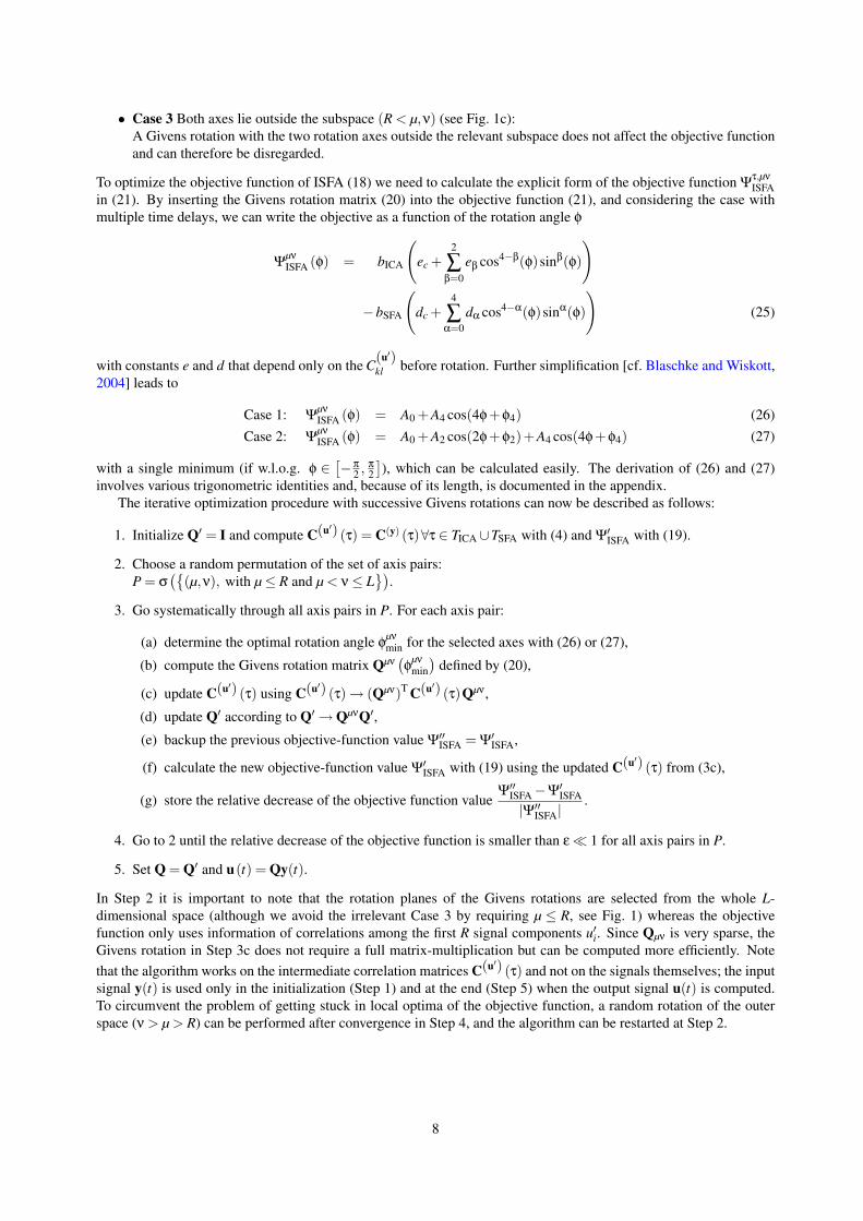
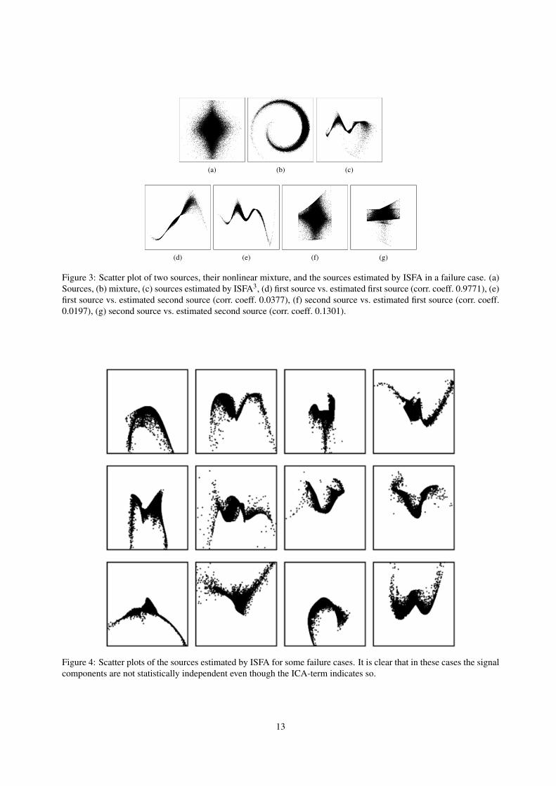
It might be possible to eliminate the failures of the first three cases by refining the algorithm, e.g. by tuning theweighting factors better or by going to higher polynomials, but Case 4 is more fundamental and requires to reconsiderthe objective function itself. In this latter case, the signals extracted by ISFA appear to be both slower and moremutually independent than the original sources. However, scatter plots of the estimated sources reveal that they are notstatistically independent at all, but often one is largely a function of the other, see Figures 3 and 4. Thus the ICA partof the objective function is not strong enough to assure statistical independence of the estimated sources. The cross-correlation functions shown in Figure 5 indicate that this problem is not due to the specific choice of the time delays,because the time-delayed cross-correlations of the estimated sources (mean ± std = 0± 0.0028) are overall smallerthan the ones of the original sources (0±0.0066). Even using different or more time delays, such dataset would havebeen processed incorrectly. We conclude that any measure of independence based on time-delayed correlations wouldbe insufficient in our context.

Figure 5 suggested to us that sources with a large standard deviation of their cross-correlation function might beparticularly difficult to separate with our ISFA algorithm. We tested this hypothesis but did not find a significantcorrelation with the failure cases. For an expansion with polynomials of degree three even linear regression fails ifthe standard deviation of the first signal, which goes along the spiral, is large. For polynomials of degree five linearregression always worked in our examples but we suspected that separation might still be more difficult for sourceswith large standard deviation, but again, we did not find a significant correlation with the failure cases.

We argue here that the failures must be attributed to the weakness of the ICA-term in the objective function. Ifthe SFA-term were too weak, it could happen that all output signal components are truly statistically independent butat least some of them are too quickly varying, so that they are not correlated to the sources but to some nonlinearlydistorted version of the sources, something we did not observe. Also the success in detecting the failure cases basedon higher-order cumulants (see next section) indicates that the failures are due to the ICA-term.

5.5 Unsupervised detection of failure casesA failure rate of about 30% (or even up to 50% for ISFA3 if one also counts the cases in which even linear regres-sion was not able to recover the sources) is obviously not acceptable, unless one can detect the failure cases in anunsupervised manner. We use the weighted sum over the third and fourth order cross-cumulants,

Ψ34(u) :=13! ∑

i jk 6=iii

(C(u)

i jk

)2+

14! ∑

i jkl 6=iiii

(C(u)

i jkl

)2, (34)

12

(a) (b) (c)

(d) (e) (f) (g)

Figure 3: Scatter plot of two sources, their nonlinear mixture, and the sources estimated by ISFA in a failure case. (a)Sources, (b) mixture, (c) sources estimated by ISFA3, (d) first source vs. estimated first source (corr. coeff. 0.9771), (e)first source vs. estimated second source (corr. coeff. 0.0377), (f) second source vs. estimated first source (corr. coeff.0.0197), (g) second source vs. estimated second source (corr. coeff. 0.1301).

Figure 4: Scatter plots of the sources estimated by ISFA for some failure cases. It is clear that in these cases the signalcomponents are not statistically independent even though the ICA-term indicates so.

13

-10 -8 -6 -4 -2 0 2 4 6 8 10τ [×105]

-0.03

-0.02

-0.01

0.00

0.01

0.02

0.03

C(τ)

(a)

-10 -8 -6 -4 -2 0 2 4 6 8 10τ [×105]

-0.03

-0.02

-0.01

0.00

0.01

0.02

0.03

C(τ)

(b)

Figure 5: Cross-correlation functions of a failure case: (a) cross-correlation function of the original sources, (b) cross-correlation function of the estimated sources. Same dataset as in Fig. 3.

as an independent measure of statistical independence to indicate with high values those cases in which the second or-der ICA-term has failed to yield independent output signal components. The factors 1

3! and 14! arise from an expansion

of the Kullback-Leibler divergence in u, which provides a rigorous derivation of this criterion [Comon, 1994; McCul-lagh, 1987]. The Receiver Operating Characteristic (ROC) curves in Figure 6 show that Ψ34(u) is a good measureof success. These tests also included the cases where linear regression was not able to recover the sources. The areaunder the ROC curves is 0.952 and 0.988 for ISFA3 and ISFA5, respectively.

6 ConclusionIn the work presented here we have addressed the problem of nonlinear blind source separation. It is known thatin contrast to the linear case statistical independence alone is not a sufficient criterion for separating sources from anonlinear mixture; additional criteria are needed to solve the problem of selecting the true sources (or good repre-sentatives thereof) from the many possible output signal components that would be statistically independent of othercomponents. We claim here that for source signals with significant autocorrelations for time delay one temporal slow-ness is a good criterion to solve this selection problem, because the slow components are those most likely related tothe true sources by an invertible transformation; non-invertible transformations would typically lead to more quicklyvarying components.

Based on this assumption, we have derived an objective function that combines a term from second-order Inde-pendent Component Analysis (ICA) with a term derived from Slow Feature Analysis (SFA). Optimization of the newobjective function is achieved by successive Givens rotations, a method often used in context of ICA. We refer to theresulting algorithm as independent Slow Feature Analysis (ISFA) to indicate the combination of ICA and SFA.

The algorithm is somewhat unusual in that only a small submatrix of large time-delayed correlation matrices arebeing diagonalized by the Givens rotations (usually the full matrices are being diagonalized). This opens the questionof the uniqueness of the solution. Using randomly generated pseudo-correlation-matrices we have found that indeeda minimum number of time delays is needed to obtain unique and meaningful solutions. For instance, if the upper left2×2-submatrix of 9×9-matrices have to be diagonalized, at least 18 such matrices are needed to obtain a meaningful

14

0 0.2 0.4 0.6 0.8 1False positive rate

0

0.2

0.4

0.6

0.8

1

True

pos

itive

rate

Figure 6: ROC curves for the test of successful source separation based on Ψ34(u), the weighted sum of third- andfourth-order cross-cumulants. The area under the curves is 0.952 and 0.988 for ISFA3 (dashed line) and ISFA5 (solidline), respectively.

solution that would be very unlikely to emerge by accident; with 17 matrices on the other hand good diagonalizationcan be achieved reliably even for random symmetric matrices. With (sufficiently many) surrogate matrices, structuredsuch that they have a unique solution, we have subsequently verified that the algorithm reliably converges to the correctsolution.

With tests on quite an extreme nonlinear mixture of two audio signals we have shown that ISFA is indeed able toperform nonlinear blind source separation, often with high precision. However, in about 30% of the cases in whichthe true sources could have been extracted with the nonlinearity used (as verified by regression) ISFA failed to extractthem. In many of these cases the extracted signals were actually better than the original sources in both the SFA-termas well as the ICA-term of the objective function. This was a surprising finding for us, since it seems to contradict ourbasic assumption that a combination of slowness and statistical independence should permit reliable nonlinear blindsource separation. Closer inspection, however, has revealed that the extracted output signal components only appear tobe statistically independent in terms of the time-delayed second-order moments but that they are often highly related,as can be seen by visual inspection (Fig. 4) and automatically detected with a measure Ψ34(u) based on higher-ordercumulants. This is not a consequence of the particular choice of time delays we have used but would be expected forany general set of time delays, as can be seen from the cross-correlation functions (Fig. 5).

We believe that two important conclusions can be drawn from these results. Firstly, the success cases indicatethat combining slowness and statistical independence is a promising approach to nonlinear blind source separation.Secondly, any measure of statistical independence based on (time-delayed) second-order moments is too weak toguarantee statistical independence in our context; it might even be too weak in any context where the dimensionalityof the space in which the signal components are searched for is significantly larger than the number of components.

For a possible theoretical account of the failure of second-order ICA in our context consider the following example.Given a symmetrically distributed source s1 the correlation between, for instance, s1 and s2

1 vanishes [Harmeling et al.,2003, sec. 4.1]. To the extent that this also holds for time-shifted versions s1(t) and s2

1(t + τ) [cf. Harmeling et al.,2003, sec. 5.4] the statistical dependence between s1 and s2

1 does not manifest itself in the time-delayed correlations.Thus, second-order ICA cannot be expected to prevent extraction of s1 and s2

1 as the estimated sources, which caneasily lead to a failure case, if s2

1 is more slowly varying than, e.g., s2 .A failure rate of 30% would render the algorithm useless if it were not possible to detect the failure cases. We

have shown that the measure Ψ34(u), which is based on higher-order cumulants, permits failure detection with highreliability; the area under the ROC curve is greater than 0.95 resulting in a true positive rate of 90% and 94% at a falsepositive rate of 5% and 10% for ISFA3 and ISFA5, respectively.

It might be possible to use Ψ34(u) not only to detect the failure cases but also to automatically tune the weight bICAgiven bSFA = 1 and to determine the number of sources. For the former one could start with a small value of bICA, sothat only the SFA-term is effective and the extracted components might not be independent, and then increase bICA, sothat the ICA-term becomes increasingly effective, until the value of Ψ34(u) drops below a certain threshold. Similarly,

15

for determining the number of sources one could start by running the algorithm with only two output components tobe extracted and successively increase the number of components. One would then stop if adding another componentwould increase Ψ34(u) significantly (which can obviously be detected only a posteriori).

More interesting, however, would be to use higher-order cumulants more directly to improve the algorithm. Forinstance, one could define a new objective function that is a combination of the SFA-term used here and an ICA-termlike Ψ34(u). Given the high reliability with which Ψ34(u) can detect failure cases, we expect better performancewith such a new objective function. However, higher-order cumulants are expensive to compute, especially for high-dimensional and long signals, so that there is probably a trade-off between reliability and computational complexity.Exploring these possibilities will be subject of our future research.

AcknowledgmentsThis work has been supported by the Volkswagen Foundation through a grant to LW for a junior research group.We thank Pietro Berkes for carefully going through all constants and Barak Pearlmutter for helpful comments. Allexamples have been implemented in Python using the Modular Toolkit for Data Processing1.

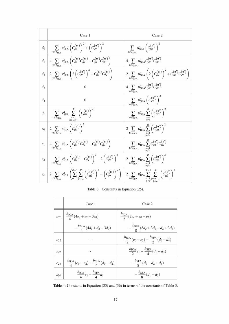
AppendixThe definitions of the constants dn and en for the expression of the objective function (25) follow directly from themultilinearity of C(u)

... (τ). They are given in Table 3. Using trigonometry we can derive simpler objective functions ofthe form

Case 1: Ψµν

ISFA(φ) = a20 + c24 cos(4φ)+ s24 sin(4φ) (35)Case 2: Ψ

µν

ISFA(φ) = a20 + c22 cos(2φ)+ s22 sin(2φ)+c24 cos(4φ)+ s24 sin(4φ) (36)

with constants defined in Table 4. In the next step these objective functions are further simplified by combining thesine term and cosine term in a single cosine term. This results in:

Case 1: Ψµν

ISFA(φ) = A0 +A4 cos(4φ+φ4) (37)Case 2: Ψ

µν

ISFA(φ) = A0 +A2 cos(2φ+φ2)+A4 cos(4φ+φ4) (38)

with constants defined in Table 5. It is easy to see why it is possible to write both objective functions (37) and (38) insuch a simple form. Firstly, the terms in (25) are products of at most four sin(φ) and cos(φ) functions, which allows,at most, a frequency of 4. Secondly, in Case 1 Ψ

µν

ISFA(φ) has a periodicity of π/2 because rotations by multiples of π/2correspond to a permutation (possibly plus sign change) of the two components. Since both components are inside thesubspace, permutations do not change the objective function and the objective function has a π/2 periodicity. Thuswe conclude that only frequencies of 0 and 4 can be present in (37). In Case 2, since one component lies outside thesubspace, an exchange of components will change the objective function (38). A rotation by multiples of π, however,which results only in a possible sign change, will leave the objective function unchanged, resulting in an objectivefunction with π-periodicity and therefore frequencies of 0, 2, and 4.

1Freely available at http://mdp-toolkit.sourceforge.net .

16

Case 1 Case 2

d0 ∑τ∈TSFA

κτSFA

(C

(u′)µµ

)2

+(

C(u′)νν

)2

∑τ∈TSFA

κτSFA

(C

(u′)µµ

)2

d1 4 ∑τ∈TSFA

κτSFA

(C

(u′)µµ C

(u′)µν −C

(u′)µν C

(u′)νν

)4 ∑

τ∈TSFA

κτSFAC

(u′)µν C

(u′)µµ

d2 2 ∑τ∈TSFA

κτSFA

(2(

C(u′)µν

)2

+C(u′)µµ C

(u′)νν

)2 ∑

τ∈TSFA

κτSFA

(2(

C(u′)µν

)2

+C(u′)µµ C

(u′)νν

)

d3 0 4 ∑τ∈TSFA

κτSFAC

(u′)µν C

(u′)νν

d4 0 ∑τ∈TSFA

κτSFA

(C

(u′)νν

)2

dc ∑τ∈TSFA

κτSFA

R

∑α=1,

α 6∈{µ,ν}

(C

(u′)αα

)2

∑τ∈TSFA

κτSFA

R

∑α=1α6=µ

(C

(u′)αα

)2

e0 2 ∑τ∈TICA

κτICA

(C

(u′)µν

)2

2 ∑τ∈TICA

κτICA

R

∑α=1α6=µ

(C

(u′)µα

)2

e1 4 ∑τ∈TICA

κτICA

(C

(u′)µν C

(u′)νν −C

(u′)µµ C

(u′)µν

)∑

τ∈TICA

κτICA

R

∑α=1α6=µ

C(u′)µα C

(u′)αν

e2 ∑τ∈TICA

κτICA

(C

(u′)µµ −C

(u′)νν

)2

−2(

C(u′)µν

)2

2 ∑τ∈TICA

κτICA

R

∑α=1α6=µ

(C

(u′)αν

)2

ec 2 ∑τ∈TICA

κτICA

(R−1

∑α=1

R

∑β>α

(C

(u′)αβ

)2

−(

C(u′)µν

)2)

2 ∑τ∈TICA

κτICA

R−1

∑α=1,α6=µ

R

∑β=α+1,

β6=µ

(C

(u′)αβ

)2

Table 3: Constants in Equation (25).

Case 1 Case 2

a20bICA

4(4ec + e2 +3e0)

bICA

2(2ec + e0 + e2)

− bSFA

4(4dc +d2 +3d0) − bSFA

8(8dc +3d0 +d2 +3d4)

c22 -bICA

2(e0− e2)−

bSFA

2(d0−d4)

s22 -bICA

2e1−

bSFA

4(d1 +d3)

c24bICA

4(e0− e2)−

bSFA

4(d0−d2) − bSFA

8(d0−d2 +d4)

s24bICA

4e1−

bSFA

4d1 − bSFA

8(d1−d3)

Table 4: Constants in Equation (35) and (36) in terms of the constants of Table 3.

17

Case 1 Case 2

A0 a20 a20

A2 -√

c222 + s2

22

A4

√c2

24 + s224

√c2

24 + s224

tan(φ2) - − s22

c22

tan(φ4) − s24

c24− s24

c24

Table 5: Constants in Equations (37) and (38) in terms of the constants of Table 4.

18

ReferencesAlmeida, L. (2004). Linear and nonlinear ICA based on mutual information - the MISEP method. Signal Processing,

84(2):231–245. Special Issue on Independent Component Analysis and Beyond.

Amari, S., Cichocki, A., and Yang, H. (1995). Recurrent neural networks for blind separation of sources. In Proc. ofthe Int. Symposium on Nonlinear Theory and its Applications (NOLTA-95), pages 37–42, Las Vegas, USA.

Babaie-Zadeh, M., Jutten, C., and Nayebi, K. (2002). A geometric approach for separating post-nonlinear mixtures.In Proc. of the XI European Signal Processing Conference (EUSIPCO 2002), pages 11–14.

Belouchrani, A., Abed Meraim, K., Cardoso, J.-F., and Éric Moulines (1997). A blind source separation techniquebased on second order statistics. IEEE Transactions on Signal Processing, 45(2):434–44.

Blaschke, T., Berkes, P., and Wiskott, L. (2006). What is the relation between independent component analysis andslow feature analysis? Neural Computation, 18(10):2495–2508.

Blaschke, T. and Wiskott, L. (2004). CuBICA: Independent component analysis by simultaneous third- and fourth-order cumulant diagonalization. IEEE Transactions on Signal Processing, 52(5):1250–1256.

Cardoso, J.-F. (2001). The three easy routes to independent component analysis; contrasts and geometry. In Proc. ofthe 3rd Int. Conference on Independent Component Analysis and Blind Source Separation, San Diego, (ICA 2001).

Cardoso, J.-F. and Souloumiac, A. (1996). Jacobi angles for simultaneous diagonalization. SIAM J. Mat. Anal. Appl.,17(1):161–164.

Comon, P. (1994). Independent component analysis, a new concept? Signal Processing, 36(3):287–314. Special Issueon Higher-Order Statistics.

Harmeling, S., Ziehe, A., Kawanabe, M., and Müller, K.-R. (2003). Kernel-based nonlinear blind source separation.Neural Computation, 15:1089–1124.

Hosseini, S. and Jutten, C. (2003). On the separability of nonlinear mixtures of temporally correlated sources. IEEESignal Processing Letters, 10(2):43–46.

Hyvärinen, A. and Pajunen, P. (1999). Nonlinear independent component analysis: existence and uniqueness results.Neural Networks, 12(3):429–439.

Jutten, C. and Karhunen, J. (2003). Advances in nonlinear blind source separation. In Proc. of the 4th Int. Symposiumon Independent Component Analysis and Blind Signal Separation, Nara, Japan, (ICA 2003), pages 245–256.

McCullagh, P. (1987). Tensor methods in statistics. Monographs on Statistics and Applied Probability. Chapmann andHall, London.

Molgedey, L. and Schuster, G. (1994). Separation of a mixture of independent signals using time delayed correlations.Physical Review Letters, 72(23):3634–3637.

Taleb, A. (2002). A generic framework for blind source separation in structured nonlinear models. IEEE Transactionson Signal Processing, 50(8):1819–1830.

Taleb, A. and Jutten, C. (1997). Nonlinear source separation: The post-nonlinear mixtures. In Proc. EuropeanSymposium on Artificial Neural Networks, Bruges, Belgium, pages 279–284.

Taleb, A. and Jutten, C. (1999). Source separation in post non linear mixtures. IEEE Transactions on Signal Process-ing, 47(10):2807–2820.

Tong, L., Liu, R., Soon, V. C., and Huang, Y.-F. (1991). Indeterminacy and identifiability of blind identification. IEEETransactions on Circuits and Systems, 38(5):499–509.

Wiskott, L. and Sejnowski, T. (2002). Slow feature analysis: Unsupervised learning of invariances. Neural Computa-tion, 14(4):715–770.

Yang, H.-H., Amari, S., and Cichocki, A. (1998). Information-theoretic approach to blind separation of sources innon-linear mixture. Signal Processing, 64(3):291–300.

19

Ziehe, A., Kawanabe, M., Harmeling, S., and Müller, K.-R. (2003). Blind separation of post-nonlinear mixtures usinglinearizing transformations and temporal decorrelation. Journal of Machine Learning Research, 4:1319–1338.

Ziehe, A. and Müller, K.-R. (1998). TDSEP – an efficient algorithm for blind separation using time structure. In Proc.of the 8th Int. Conference on Artificial Neural Networks (ICANN’98), pages 675 – 680, Berlin. Springer Verlag.

20