Improvising Jazz With Markov Chains - CiteSeerX

Improvising Jazz WithMarkov ChainsYuval Marom

This report is submitted as partial ful�lmentof the requirements for the Honours Programme of theDepartment of Computer ScienceThe University of Western Australia1997

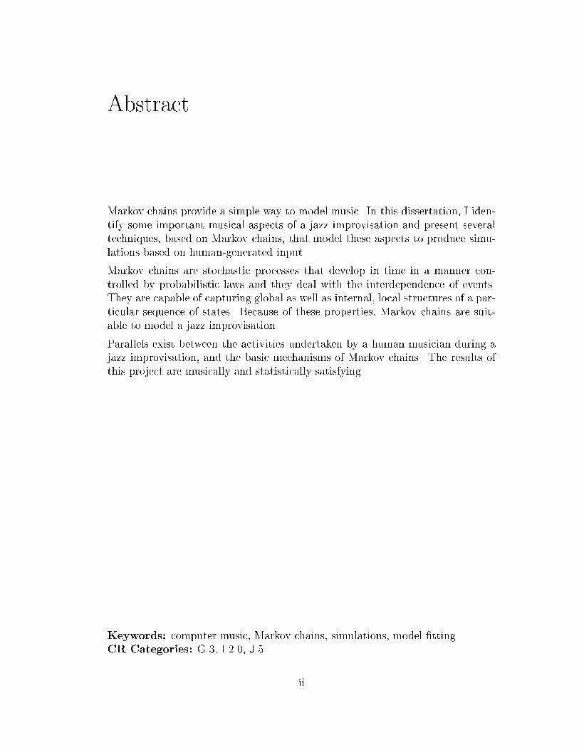
AbstractMarkov chains provide a simple way to model music. In this dissertation, I iden-tify some important musical aspects of a jazz improvisation and present severaltechniques, based on Markov chains, that model these aspects to produce simu-lations based on human-generated input.Markov chains are stochastic processes that develop in time in a manner con-trolled by probabilistic laws and they deal with the interdependence of events.They are capable of capturing global as well as internal, local structures of a par-ticular sequence of states. Because of these properties, Markov chains are suit-able to model a jazz improvisation.Parallels exist between the activities undertaken by a human musician during ajazz improvisation, and the basic mechanisms of Markov chains. The results ofthis project are musically and statistically satisfying.

Keywords: computer music, Markov chains, simulations, model �ttingCR Categories: G.3, I.2.0, J.5 ii

AcknowledgementsI would like to thank the following people:My supervisor from Mathematics, Adrian Baddeley, for his constant input andenthusiasm, which have kept me going all year.My supervisor from Computer Science, C. P. Tsang, for showing interest through-out the year, and always having new ideas (that I haven't thought of previously!)Leigh Smith, for providing me with some directions early on in the year when Ineeded it most. Without his endless bibliography (literature and software) thiswould have taken a lot more than a year.The members of Compmuse | the UWA Computer Music Research Group |for showing interest every Tuesday at 12:30 (and at other times too, of course).My parents, Murray and Irit Aitkin, for collectively being my third supervisor.Their ever present support, and especially at thesis-writing time, was invaluable.And last but de�nitely not least, my sister Dorit, who took control of thingswhen I was stressing (quite a frequent event). Much appreciated!

iii

ContentsAbstract iiAcknowledgements iii1 Introduction 11.1 Objective . . . . . . . . . . . . . . . . . . . . . . . . . . . . . . . 11.2 Musical Considerations . . . . . . . . . . . . . . . . . . . . . . . . 21.3 Approaches . . . . . . . . . . . . . . . . . . . . . . . . . . . . . . 32 Review of the Literature 52.1 Markov Chains as Stochastic Processes . . . . . . . . . . . . . . . 52.2 Automated Composition . . . . . . . . . . . . . . . . . . . . . . . 62.2.1 History . . . . . . . . . . . . . . . . . . . . . . . . . . . . . 62.2.2 Stochastic Techniques for Computer-Music Composition . 62.2.3 Composing Programs . . . . . . . . . . . . . . . . . . . . . 62.3 The Psychology of Improvisation . . . . . . . . . . . . . . . . . . 73 Methods 83.1 Mathematical Background . . . . . . . . . . . . . . . . . . . . . . 83.2 Implementation . . . . . . . . . . . . . . . . . . . . . . . . . . . . 103.3 Simple Markov Chains . . . . . . . . . . . . . . . . . . . . . . . . 123.3.1 The Initial Model | Pitch Only . . . . . . . . . . . . . . . 133.3.2 The Improved Model | Notes/Rests . . . . . . . . . . . . 133.3.3 Extensions of the Improved Model | Duration & Volume 143.3.4 The Final Model . . . . . . . . . . . . . . . . . . . . . . . 14iv

3.3.5 Interactions . . . . . . . . . . . . . . . . . . . . . . . . . . 153.3.6 Algorithms . . . . . . . . . . . . . . . . . . . . . . . . . . 163.4 Controlled Markov Chains . . . . . . . . . . . . . . . . . . . . . . 173.4.1 Hidden Markov Models . . . . . . . . . . . . . . . . . . . . 173.4.2 Controlled Markov Chains . . . . . . . . . . . . . . . . . . 183.4.3 The Final Model . . . . . . . . . . . . . . . . . . . . . . . 213.4.4 Musical Controllers . . . . . . . . . . . . . . . . . . . . . . 223.4.5 Algorithms . . . . . . . . . . . . . . . . . . . . . . . . . . 224 Results 244.1 Statistical Measures of Musical Resemblance . . . . . . . . . . . . 254.2 The Treatment of Notes and Rests . . . . . . . . . . . . . . . . . 254.3 The Signi�cance of the Underlying States . . . . . . . . . . . . . . 304.4 The Signi�cance of the Order of the Chain . . . . . . . . . . . . . 335 Conclusion and Discussion 36A Statistical Testing 40B Figures 42B.1 Multi-track output from MF2T . . . . . . . . . . . . . . . . . . . 42B.2 Distribution Plots . . . . . . . . . . . . . . . . . . . . . . . . . . . 43C Musical Excerpts 46D Original Honours Proposal 62D.1 Background . . . . . . . . . . . . . . . . . . . . . . . . . . . . . . 62D.2 Aim . . . . . . . . . . . . . . . . . . . . . . . . . . . . . . . . . . 63D.3 Methods . . . . . . . . . . . . . . . . . . . . . . . . . . . . . . . . 63

v

List of Tables4.1 Percentages of notes and rests from the original music, and from thesimulations of the naive and advanced versions. . . . . . . . . . . . . 274.2 Percentages of rest runs of length greater than 10. . . . . . . . . . . . 294.3 Converging values of the order of the chain . . . . . . . . . . . . . . 34

vi

List of Figures2.1 Memory as a mental factor of musical creation . . . . . . . . . . . 73.1 Typical output from MF2T, the MIDI-File-to-Text converter . . . . . . 113.2 An overview of the methodology . . . . . . . . . . . . . . . . . . . 113.3 An musical example with smallest note duration 18 . . . . . . . . . 123.4 The interpretation of the example by the \Pitch Only" approach . 133.5 The interpretation of the example by the \Notes/Rests" approach 143.6 The interpretation of the example by the \Duration & Volume"approach . . . . . . . . . . . . . . . . . . . . . . . . . . . . . . . . 153.7 The Simple Markov Chain approach . . . . . . . . . . . . . . . . . 153.8 A Hidden Markov Model . . . . . . . . . . . . . . . . . . . . . . . . 173.9 Two ways to conceptualize the relationship between underlyingand simple states . . . . . . . . . . . . . . . . . . . . . . . . . . . 194.1 Runs of notes and rests . . . . . . . . . . . . . . . . . . . . . . . . 254.2 \Israel" | �rst two bars. . . . . . . . . . . . . . . . . . . . . . . . 264.3 The interpretation of \Israel" by the naive approach . . . . . . . . 264.4 The interpretation of \Israel" by the advanced approach . . . . . 264.5 Partial simulation of the naive model, based on \Israel" . . . . . . 264.6 Partial simulation of the advanced model, based on \Israel" . . . 274.7 Plot of Note Runs. . . . . . . . . . . . . . . . . . . . . . . . . . . . 284.8 Plot of Rest Runs. . . . . . . . . . . . . . . . . . . . . . . . . . . . 294.9 \Jules1" | �rst bar under each underlying drum pattern . . . . . 314.10 The interpretation of \Jules 1" by the naive approach . . . . . . . 314.11 The interpretation of \Jules 1" by the controlled approach . . . . 324.12 Partial simulation of the simple model, based on \Jules 1" . . . . 324.13 Partial simulation of the controlled model, based on \Jules1" . . . 33vii

4.14 Convergence of the number of unique tuples in the data . . . . . . 35B.1 Multi-track output from MF2T corresponding to the presence ofunderlying states . . . . . . . . . . . . . . . . . . . . . . . . . . . 42B.2 Distribution of pitch . . . . . . . . . . . . . . . . . . . . . . . . . 43B.3 Distribution of duration . . . . . . . . . . . . . . . . . . . . . . . 44B.4 Distribution of volume . . . . . . . . . . . . . . . . . . . . . . . . 44B.5 Distribution of note runs . . . . . . . . . . . . . . . . . . . . . . . 45B.6 Distribution of rest runs . . . . . . . . . . . . . . . . . . . . . . . 45

viii

CHAPTER 1IntroductionAutomated composition is a �eld of computer music that deals with the problemof designing a procedure that will imitate the compositional process of a humancomposer. As in other forms of art, such as sculpture and painting, the study ofautomated composition seeks to �nd out whether the process of artistic creationis mathematical in nature. The answer to this need not be a simple yes or no.The problem can therefore be reformulated as one of �nding the extent of the ex-istence of mathematics in the process of artistic creation.Musical composition is one of many aspects of human behavior and so any con-clusions drawn from attempts to model it may be important in the study of Arti-�cial Intelligence and Cognitive Science. From a practical point of view, a modelof any music can be used to generate music automatically | uses of this mightbe found in �lms, television, and elsewhere.The words \composition" and \improvisation" will be interchanged throughoutthis dissertation. Improvisation is simply a sub-class of composition. I do notintend to go into full details of the musical di�erences between these two activ-ities, but a brief discussion is presented in Chapter 2. It will become apparentwhen I present the techniques that \improvisation" is a more precise descriptionof the process we are trying to automate.As the title of the project suggests, the musical application used here is jazz.This gives us another indication that we are dealing with improvisation, as jazzis mostly improvised.1.1 ObjectiveWe can identify at least two main approaches for generating computer-composedmusic. One approach is a \self-contained" composing procedure that creates themusic solely through its algorithms. In other words, a procedure that does notdepend on any input is used to synthesize new, truly original, music. The secondapproach is a procedure that creates the music by following some guidelines, or1

1. Introduction 2characteristics, that are inherent in an existing piece of music. In contrast withthe �rst approach, this approach can be regarded as trying to reproduce music,or style.The work presented in this dissertation follows the second approach. The objec-tive of this project is, therefore, to generate simulations based on existing jazzpieces. In statistical terms, we start with existing data, �t a model, and then usethe model to simulate new data.1.2 Musical ConsiderationsBefore trying to formalize musical composition, one must �rst �nd out what arethe main factors that a�ect the process of composing. Then, one must �nd amodel that will deal with as many of these factors as possible at the same time.A computer program that simply reproduces a particular piece of music is obvi-ously not an adequate one, because this will not be regarded as an original com-position. A model of composition in most musical genres, and particularly jazz,must consider two issues:1. It must capture the style of the composer. If the model cannot capture style,then we have to question its appropriateness. Style is what distinguishesone composer from another, one time-period from another, one genre fromanother etc. It is something that must be inherited by the model.2. It should allow for spontaneous actions. It can be argued that the extentto which listeners �nd a particular piece of music interesting is signi�cantlya�ected by the piece's unpredictability (though they are not always awareof it). This point is important if we wish the result to be original, and tomaintain audience interest.Notice that the �rst consideration requires a copying mechanism, whereas thesecond one requires a degree of randomness, and these con ict somewhat. Themodel, therefore, must also include a mechanism for determining and controllingthe trade-o� between the two. These two considerations can be thought of as thefactors that a�ect the process of composition: a composer makes decisions aboutwhere the music will go by following particular guidelines according to his/herstyle, and also by considering new, original, and unanticipated possibilities.It is relatively easy to �nd a simple solution that models one of the above twoproperties. In this dissertation I present a tool, called a Markov chain, for mod-eling both properties at the same time. Markov chains are used to model tempo-ral dependence between events, or states, of processes. Such processes are calledstochastic processes. It is my view that these kinds of processes describe someof the characteristics of a jazz improvisation, such as the ones mentioned above.

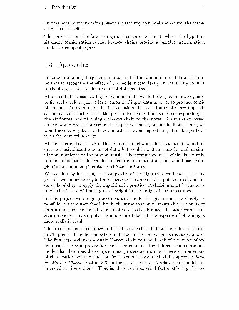
1. Introduction 3Furthermore, Markov chains present a direct way to model and control the trade-o� discussed earlier.This project can therefore be regarded as an experiment, where the hypothe-sis under consideration is that Markov chains provide a suitable mathematicalmodel for composing jazz.1.3 ApproachesSince we are taking the general approach of �tting a model to real data, it is im-portant to recognize the e�ect of the model's complexity on the ability to �t itto the data, as well as the amount of data required.At one end of the scale, a highly realistic model would be very complicated, hardto �t, and would require a large amount of input data in order to produce sensi-ble output. An example of this is to consider the n attributes of a jazz improvi-sation, consider each state of the process to have n dimensions, corresponding tothe attributes, and �t a single Markov chain to the states. A simulation basedon this would produce a very realistic piece of music, but in the �tting stage, wewould need a very large data set in order to avoid reproducing it, or big parts ofit, in the simulation stage.At the other end of the scale, the simplest model would be trivial to �t, would re-quire an insigni�cant amount of data, but would result in a nearly random sim-ulation, unrelated to the original music. The extreme example of this is a purelyrandom simulation: this would not require any data at all, and would use a sim-ple random number generator to choose the states.We see that by increasing the complexity of the algorithm, we increase the de-gree of realism achieved, but also increase the amount of input required, and re-duce the ability to apply the algorithm in practice. A decision must be made asto which of these will have greater weight in the design of the procedures.In this project we design procedures that model the given music as closely aspossible, but maintain feasibility in the sense that only \reasonable" amounts ofdata are needed, and results are relatively easily obtained. In other words, de-sign decisions that simplify the model are taken at the expense of obtaining amore realistic result.This dissertation presents two di�erent approaches that are described in detailin Chapter 3. They lie somewhere in between the two extremes discussed above.The �rst approach uses a single Markov chain to model each of a number of at-tributes of a jazz improvisation, and then combines the di�erent chains into onemodel that describes the compositional process as a whole. These attributes arepitch, duration, volume, and note/rest events. I have labelled this approach Sim-ple Markov Chains (Section 3.3) in the sense that each Markov chain models itsintended attribute alone. That is, there is no external factor a�ecting the de-

1. Introduction 4velopment of the model, not even a connection between the di�erent attributes.This is the main limitation of the approach. It assumes independence betweenthe di�erent attributes, as the modeling of each is performed separately.The second approach is an extension of the �rst one, where there is an underlyingsequence of states controlling the behavior of the Markov chains, which I thereforecall Controlled Markov Chains (Section 3.4). These states can be thought of assome kinds of external conditions that have a global e�ect on the improvisation.

CHAPTER 2Review of the Literature2.1 Markov Chains as Stochastic ProcessesSignal modelling can be categorized into two classes: deterministic and statistical[13], though the two are by no means mutually exclusive. In deterministic mod-elling we might refer to characterization of a signal with known pre-determinedproperties. In statistical modelling we might refer to stochastic processes, suchas Gaussian, Poisson, and Markov processes [13], to characterize a signal that isunpredictable, to some extent.The theory of stochastic processes applies to �elds such as statistical physics,population growth, communication and control theory, weather forecasting, timeseries analysis [15], and speech processing [13]. These are processes that developin time in a manner controlled by probabilistic laws. They deal with the behav-ior of a collection of random variables and their interdependence [15].A Markov process is a stochastic process whose future state is only dependent onthe current state, and not on any previous states. A Markov chain is a Markovprocess operating over a �nite (countable) set of states. It is used to model reallife situations such as: queue servicing, population growth, system maintenance(operation, breakdown, and repair of a system), and written language (text anal-ysis) [15].In fact, a speci�c application of Markov chains to text analysis has provided theinspiration for this project. I am referring to a program called \Babble" [7] thatwas written by one of my supervisors, Adrian Baddeley. This program takes atext �le as input and �ts a Markov chain to the words or characters in the text, asspeci�ed by the user. It then simulates the Markov chain to give a new sequenceof words or characters. One can �nd many parallels of text and music, and so itseems that this technique could be applied to music. One such parallel is to treatthe states of the Markov chain as notes, rather than words (or characters).

5

2. Review of the Literature 62.2 Automated Composition2.2.1 HistoryMany recorded attempts at automating the process of composition exist through-out musical history. However, these e�orts have met with continuing resistancefrom music critics until the latter half of the current century. Charles Ames hasconducted an extensive survey of the wide range of techniques that have beenemployed from 1956 to 1986 [4] in attempts to capture those characteristics thatmake a particular musical piece so unique. He argues that prior to this period, re-searchers have not been able to even address the fundamental assumptions aboutthe nature of creativity and the aesthetic purposes of composition, and hence itis not surprising that such e�orts have met with constant criticisms.Arguably the most in uential contributor to the �eld of automated compositionhas been Iannis Xenakis who argued the need for non-deterministic approaches.He published his ideas in 1971 in a book called \Formalized Music" [19], whichis frequently cited in the literature.2.2.2 Stochastic Techniques for Computer-Music CompositionPeople have the misconception that statistics is purely about random processes.Jones [12] dismisses critics' concerns that stochastic techniques lack controllabil-ity in composition, and argues that in some cases they can produce results thatsound far more \ordered" than deterministic systems.Stochastic techniques have the distinct advantage over other compositional ap-proaches in that they can produce unanticipated possibilities and \fuzzy edges"[12]. This has the e�ect of \humanizing" computer-generated music, which is fre-quently criticized for sounding too arti�cial.The uses of Markov chains in automated composition have been surveyed in an-other article by Ames [5]. The majority of them start with a model and try tocreate a particular style of music, by setting the parameters of the model. Asmentioned in the previous chapter, the approach of this project is di�erent. Westart with real music, build a model based on it by estimating the parametersfrom the data, and then try to re-create the style through the new composition.Furthermore, in this project I investigate di�erent uses of the Markov chain, andtry to extend its traditional, simplistic implementation.2.2.3 Composing ProgramsMany musical programs exist, and many more will be written, which include com-posing facilities that require full user interaction, no user interaction, and every

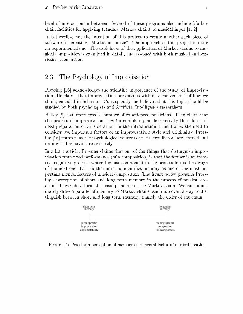
2. Review of the Literature 7level of interaction in between. Several of these programs also include Markovchain facilities for applying standard Markov chains to musical input [1, 2].It is therefore not the intention of this project to create another such piece ofsoftware for creating \Markovian music". The approach of this project is morean experimental one. The usefulness of the application of Markov chains to mu-sical composition is examined in detail, and assessed with both musical and sta-tistical conclusions.2.3 The Psychology of ImprovisationPressing [16] acknowledges the scienti�c importance of the study of improvisa-tion. He claims that improvisation presents us with a \clear version" of how wethink, encoded in behavior. Consequently, he believes that this topic should bestudied by both psychologists and Arti�cial Intelligence researchers.Bailey [8] has interviewed a number of experienced musicians. They claim thatthe process of improvisation is not a completely ad hoc activity that does notneed preparation or consideration. In the introduction, I mentioned the need toconsider two important factors of an improvisation: style and originality. Press-ing [16] states that the psychological sources of these two factors are learned andimprovised behavior, respectively.In a later article, Pressing claims that one of the things that distinguish impro-visation from �xed performance (of a composition) is that the former is an itera-tive cognitive process, where the last component in the process forms the designof the next one [17]. Furthermore, he identi�es memory as one of the most im-portant mental factors of musical composition. The �gure below presents Press-ing's perception of short and long term memory in the process of musical cre-ation. These ideas form the basic principle of the Markov chain. We can imme-diately draw a parallel of memory to Markov chains, and moreover, a way to dis-tinguish between short and long term memory, namely the order of the chain.long term

training specificcomposition

following orders

memoryshort termmemory

piece specificimprovisation

unpredictabilityFigure 2.1: Pressing's perception of memory as a mental factor of musical creation

CHAPTER 3Methods3.1 Mathematical BackgroundDe�nition: A kth order Markov chain (MC) is a stochastic process fXiji =1 : : : ng with observed values fxiji = 1 : : : ng, which operates over a �nite set ofdiscrete states, such thatProb(Xi = xijXi�1 = xi�1; :::; X1 = x1)= Prob(Xi = xijXi�1 = xi�1; :::; Xi�k = xi�k).That is, the state of the chain at time i is dependent only on the previous k states[15].To clarify this dependence property, let us look at a simple case: a �rst orderMarkov chain. The state of the chain at any time is dependent only on its pre-vious state:Prob(Xi = xijXi�1 = xi�1; :::; X1 = x1) = Prob(Xi = xijXi�1 = xi�1).A homogeneous Markov chain is one where the probabilities above do not de-pend on time | they are homogeneous with time. The Markov chains used inthis project are taken to be homogeneous.As mentioned in the de�nition, we are dealing with a sequence of discrete states,coming from a �nite state space. We consider transitions between states, andassociate a probability for each unique transition. From the de�nition we knowthat the probability that the chain will \jump" from state i to state j can be de-termined through our knowledge of the chain's previous k states only. The tran-sition probabilities are stored in a transition probability matrix.One way of estimating the transition probabilities from the data is to use the ob-served frequencies of the transitions. This technique is demonstrated below for a�rst order Markov chain with state space consisting of the letters of the Englishalphabet. 8

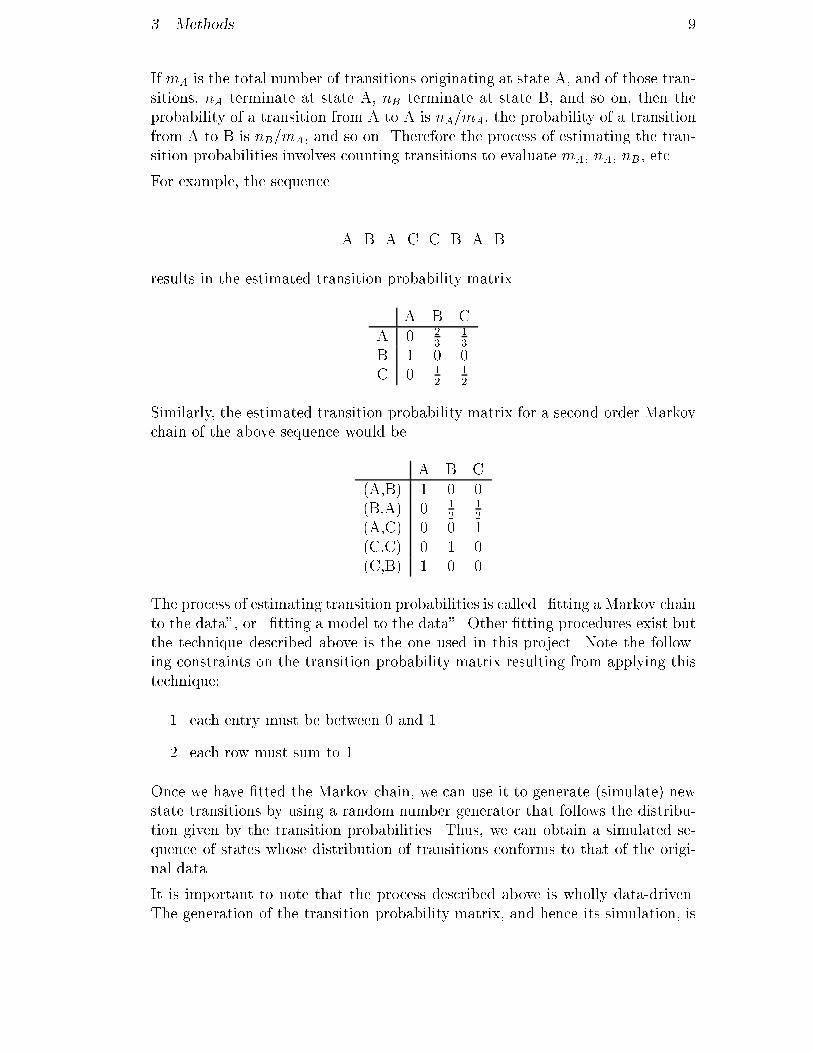
3. Methods 9If mA is the total number of transitions originating at state A, and of those tran-sitions, nA terminate at state A, nB terminate at state B, and so on, then theprobability of a transition from A to A is nA=mA, the probability of a transitionfrom A to B is nB=mA, and so on. Therefore the process of estimating the tran-sition probabilities involves counting transitions to evaluate mA, nA, nB, etc.For example, the sequence A B A C C B A Bresults in the estimated transition probability matrixA B CA 0 23 13B 1 0 0C 0 12 12Similarly, the estimated transition probability matrix for a second order Markovchain of the above sequence would be A B C(A,B) 1 0 0(B,A) 0 12 12(A,C) 0 0 1(C,C) 0 1 0(C,B) 1 0 0The process of estimating transition probabilities is called \�tting a Markov chainto the data", or \�tting a model to the data". Other �tting procedures exist butthe technique described above is the one used in this project. Note the follow-ing constraints on the transition probability matrix resulting from applying thistechnique:1. each entry must be between 0 and 12. each row must sum to 1.Once we have �tted the Markov chain, we can use it to generate (simulate) newstate transitions by using a random number generator that follows the distribu-tion given by the transition probabilities. Thus, we can obtain a simulated se-quence of states whose distribution of transitions conforms to that of the origi-nal data.It is important to note that the process described above is wholly data-driven.The generation of the transition probability matrix, and hence its simulation, is

3. Methods 10based on local patterns in the data (for example, only states in the input statespace can be produced in the simulation). The simulation of the Markov chainwill replicate those local patterns in the original data, where this is a�ected bythe order of the chain. On a more global scale, however, the simulation is a new,di�erent sequence of states where, again, the extent of this is a�ected by the orderof the chain. A high order Markov chain would capture large sized local patternsin the data and hence produce a simulation that is globally similar to the origi-nal data. In comparison, a lower order Markov chain would capture smaller sizedlocal patterns and produce a simulation that is globally less similar to the data.3.2 ImplementationBefore starting to analyze music, one needs to be able to represent it. Since wewish to automate the procedure, the computer must be able to recognize the rep-resentation we use. The Musical Instrument Digital Interface (MIDI) format isone such way of storing and manipulating music in a computer.The �rst thing we need to do is convert the music into a form that we can ma-nipulate, in order to extract the information we need. There exist many softwarepackages for handling and manipulating MIDI �les. I used a program called MF2T(MIDI File to Text) [18] which converts a MIDI �le to a text �le. It is writtenin the C programming language and runs under the Unix operating system. Atypical output of this program is given in Figure 3.1. This output is very conve-nient for data extraction.The �rst line indicates the beginning of the �le. The last piece of information onthat line tells us that the duration of the time signature is 120. The third line tellsus what the time signature is, in this case 4/4. Hence, the duration of a wholenote (4/4) is 120. The fourth and �fth lines contain information about other pa-rameters not important to us here. \MTrk" indicates the beginning of the trackand each line in the output below it represents information for one note event.The �rst column gives a time stamp of the event; the second column indicateswhether it was a note-on or note-o�; the third column indicates the pitch of thenote; and the �nal fourth column indicates the velocity with which the note wasplayed. From this information we can deduce the duration of each note by com-paring note-on and note-o� times; we can deduce pitch and velocity directly fromthe output; and we can deduce rests also by comparing note-on and note-o� times.Now that we have transformed the music into a suitable form, we can feed it tothe �tting procedure which produces a �tted model. The model will produce asimulation that we can then transform back to MIDI format by the reverse pro-gram to MF2T, called T2MF (Text to MIDI File). This process is shown in Fig-ure 3.2 and it identi�es the �tting procedure and the simulation procedure. Thedotted region signi�es where the overall procedure is dependent on the approachwe are taking, as described in the following two sub-sections.

3. Methods 11MFile 0 1 1200 Meta Copyright ``Copyright 1997 by Yuval Marom''0 TimeSig 4/4 24 80 Par ch=1 c=7 v=1000 Par ch=1 c=10 v=64MTrk0 On n=f6 v=7830 Off n=f6 v=030 On n=g6 v=8590 Off n=g6 v=090 On n=g6 v=82105 Off n=g6 v=0105 On n=b6 v=79120 Off n=b6 v=0120 On n=c7 v=92150 Off n=c7 v=0180 On n=a6 v=86225 Off n=a6 v=0240 On n=g6 v=70360 Off n=g6 v=0TrkEndFigure 3.1: Typical output from MF2T, the MIDI-File-to-Text converterinput

MF2T T2MFmodel

simulatemodel

extractsequences sequences

fitting simulation

probability

matricesof statessequences

simulatedsequences

transition

MIDI file file

text

fitmodel

filetext MIDI

fileof states

simulation

converge

Figure 3.2: An overview of the methodology. The left part is the �tting stage; the rightpart is the simulation stage. The dotted region is dependent on the approach.The two approaches use the information from MF2T in a very similar fashion,with minor di�erences. I have written functions in the C programming language,which use the output from MF2T to extract the sequences described in the fol-lowing sections. For example, a sequence of pitches extracted from the outputshown in Figure 3.1 would be `f6', `g6', `g6', `b6', `c7', `a6', `g6' (the characterrepresents the pitch; the number represents the octave number).Once these sequences are created, we can �t Markov chains to them and simu-

3. Methods 12late, as described in the previous section. I have written functions in S-Plus�that achieve both these tasks.The simulated sequences need to be converged back into one single �le, with linesof note-event information as shown in Figure 3.1, which will serve as input toT2MF. I have written functions in S-Plus that perform this task by combining in-formation from several sequences (pitch, duration, etc.).The two approaches use slightly di�erent C and S-Plus code to perform the spe-ci�c tasks. The algorithms are described brie y in the sections correspondingto these approaches. All the algorithms have been written by the author exceptwhere mentioned otherwise.3.3 Simple Markov ChainsIn this section I describe the �rst approach employed in this project. The variousstages of the development of the model are presented �rst, and the �nal modelis then discussed.I refer to the various Markov chains in this section as \simple" in the sense thatthey are at the top level of the �tting and simulation process. That is, there isno external factor a�ecting the behaviour of these chains. Furthermore, there isno interaction between the various sub-models of the �nal model. The issue ofinteraction is dealt with brie y towards the end of this section, where I remarkthat one could argue that an interaction does exist.A small example is used to illustrate the ideas in this section and it is shown inFigure 3.3. It represents the same piece of music that is depicted in Figure 3.1.G 44 ! " !��! ! > ! . ? #Pitch: F G G B C A GDuration: 14 12 18 18 14 14 38 18 1Velocity: 78 85 82 79 92 86 70Figure 3.3: An example with smallest note duration 18 . The pitch and velocities of thenotes, and the durations of the notes and rests, are listed. This excerpt corresponds tothe same piece of music depicted in Figure 3.1�S-Plus [3, 9] is a statistical, data-analysis, programming language

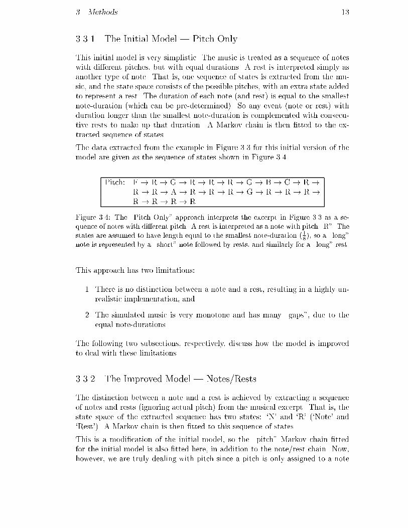
3. Methods 133.3.1 The Initial Model | Pitch OnlyThis initial model is very simplistic. The music is treated as a sequence of noteswith di�erent pitches, but with equal durations. A rest is interpreted simply asanother type of note. That is, one sequence of states is extracted from the mu-sic, and the state space consists of the possible pitches, with an extra state addedto represent a rest. The duration of each note (and rest) is equal to the smallestnote-duration (which can be pre-determined). So any event (note or rest) withduration longer than the smallest note-duration is complemented with consecu-tive rests to make up that duration. A Markov chain is then �tted to the ex-tracted sequence of states.The data extracted from the example in Figure 3.3 for this initial version of themodel are given as the sequence of states shown in Figure 3.4.Pitch: F ! R ! G ! R ! R ! R ! G ! B ! C ! R !R ! R ! A ! R ! R ! R ! G ! R ! R ! R !R ! R ! R ! RFigure 3.4: The \Pitch Only" approach interprets the excerpt in Figure 3.3 as a se-quence of notes with di�erent pitch. A rest is interpreted as a note with pitch \R". Thestates are assumed to have length equal to the smallest note-duration (18), so a \long"note is represented by a \short" note followed by rests, and similarly for a \long" rest.This approach has two limitations:1. There is no distinction between a note and a rest, resulting in a highly un-realistic implementation, and2. The simulated music is very monotone and has many \gaps", due to theequal note-durations.The following two subsections, respectively, discuss how the model is improvedto deal with these limitations.3.3.2 The Improved Model | Notes/RestsThe distinction between a note and a rest is achieved by extracting a sequenceof notes and rests (ignoring actual pitch) from the musical excerpt. That is, thestate space of the extracted sequence has two states: `N' and `R' (`Note' and`Rest'). A Markov chain is then �tted to this sequence of states.This is a modi�cation of the initial model, so the \pitch" Markov chain �ttedfor the initial model is also �tted here, in addition to the note/rest chain. Now,however, we are truly dealing with pitch since a pitch is only assigned to a note

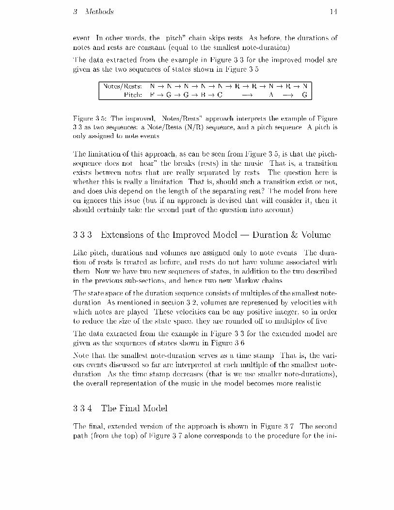
3. Methods 14event. In other words, the \pitch" chain skips rests. As before, the durations ofnotes and rests are constant (equal to the smallest note-duration).The data extracted from the example in Figure 3.3 for the improved model aregiven as the two sequences of states shown in Figure 3.5.Notes/Rests: N ! N ! N ! N ! N ! R ! R ! N ! R ! NPitch: F ! G ! G ! B ! C �! A �! GFigure 3.5: The improved, \Notes/Rests" approach interprets the example of Figure3.3 as two sequences: a Note/Rests (N/R) sequence, and a pitch sequence. A pitch isonly assigned to note events.The limitation of this approach, as can be seen from Figure 3.5, is that the pitch-sequence does not \hear" the breaks (rests) in the music. That is, a transitionexists between notes that are really separated by rests. The question here iswhether this is really a limitation. That is, should such a transition exist or not,and does this depend on the length of the separating rest? The model from hereon ignores this issue (but if an approach is devised that will consider it, then itshould certainly take the second part of the question into account).3.3.3 Extensions of the Improved Model | Duration & VolumeLike pitch, durations and volumes are assigned only to note events. The dura-tion of rests is treated as before, and rests do not have volume associated withthem. Now we have two new sequences of states, in addition to the two describedin the previous sub-sections, and hence two new Markov chains.The state space of the duration sequence consists of multiples of the smallest note-duration. As mentioned in section 3.2, volumes are represented by velocities withwhich notes are played. These velocities can be any positive integer, so in orderto reduce the size of the state space, they are rounded o� to multiples of �ve.The data extracted from the example in Figure 3.3 for the extended model aregiven as the sequences of states shown in Figure 3.6.Note that the smallest note-duration serves as a time stamp. That is, the vari-ous events discussed so far are interpreted at each multiple of the smallest note-duration. As the time stamp decreases (that is we use smaller note-durations),the overall representation of the music in the model becomes more realistic.3.3.4 The Final ModelThe �nal, extended version of the approach is shown in Figure 3.7. The secondpath (from the top) of Figure 3.7 alone corresponds to the procedure for the ini-

3. Methods 15Notes/Rests: N ! N ! N ! N ! N ! R ! R ! N ! R ! NPitch: F ! G ! G ! B ! C �! A �! GDuration: 14 ! 12 ! 18 ! 18 ! 14 �! 38 �! 1Volume: 80 ! 85 ! 80 ! 80 ! 90 �! 85 �! 70Figure 3.6: The �nal, extended version of the approach interprets the example of Fig-ure 3.3 as four sequences: the �rst two are the same as the ones interpreted by the im-proved approach (see Figure 3.5). The third is a duration sequence whose states aremultiples of the smallest note-duration (in this case 18 ). The fourth is a velocity se-quence whose states are integers rounded o� to multiples of �ve. Durations and veloc-ities are only assigned to note eventstial model (Section 3.3.1), and the top two paths of Figure 3.7 correspond to theprocedure for the improved model (Section 3.3.2).simulatedsequenceof states

probability

matrix

transition

of statessequence

simulationinput

N/R

duration

volume

pitch

convergesimulate1sep simple

Figure 3.7: The Simple Markov Chain approach. This �gure corresponds to the dot-ted region in Figure 3.2 with this approach3.3.5 InteractionsThe representation of the simulation process shown in Figure 3.7 clearly demon-strates that there are no interactions between the various aspects of the musicdiscussed so far. Once the information is extracted from the data and separatedinto the four parts, each part is dealt with separately.The musical meaning of this is that the decision of what to play next (and how),regarding a particular aspect, is not a�ected by anything that currently charac-terizes the music, except for that aspect. For example, the pitch \selector" can-not \hear" current patterns of note and rest runs, does not know the durationof the note about to be played, or how loud (or soft) it will be played. Theseare only some examples of the interactions between the aspects of the music. Ofcourse, there are many more.It can be argued that the note/rest states do have an e�ect on the pitch, dura-tion, and volume states. The note/rest Markov chain determines whether a noteor rest is played. Since pitch, duration, and volume (velocity) are only assigned

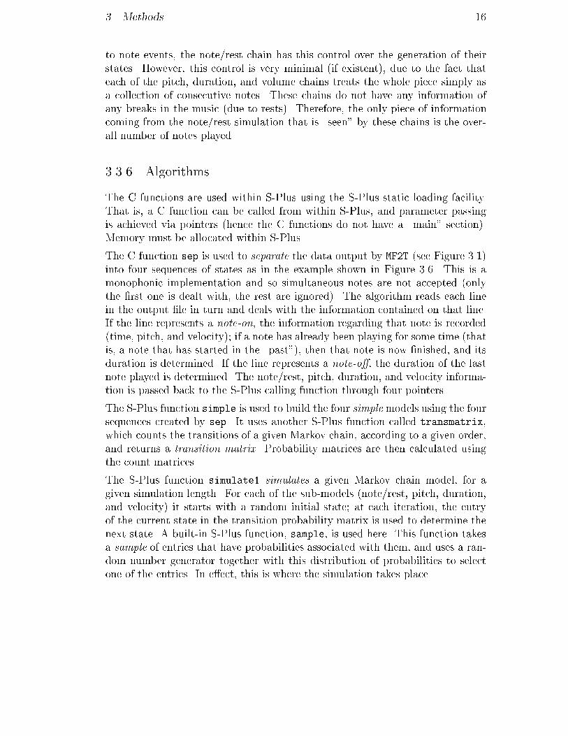
3. Methods 16to note events, the note/rest chain has this control over the generation of theirstates. However, this control is very minimal (if existent), due to the fact thateach of the pitch, duration, and volume chains treats the whole piece simply asa collection of consecutive notes. These chains do not have any information ofany breaks in the music (due to rests). Therefore, the only piece of informationcoming from the note/rest simulation that is \seen" by these chains is the over-all number of notes played.3.3.6 AlgorithmsThe C functions are used within S-Plus using the S-Plus static loading facility.That is, a C function can be called from within S-Plus, and parameter passingis achieved via pointers (hence the C functions do not have a \main" section).Memory must be allocated within S-Plus.The C function sep is used to separate the data output by MF2T (see Figure 3.1)into four sequences of states as in the example shown in Figure 3.6. This is amonophonic implementation and so simultaneous notes are not accepted (onlythe �rst one is dealt with, the rest are ignored). The algorithm reads each linein the output �le in turn and deals with the information contained on that line.If the line represents a note-on, the information regarding that note is recorded(time, pitch, and velocity); if a note has already been playing for some time (thatis, a note that has started in the \past"), then that note is now �nished, and itsduration is determined. If the line represents a note-o�, the duration of the lastnote played is determined. The note/rest, pitch, duration, and velocity informa-tion is passed back to the S-Plus calling function through four pointers.The S-Plus function simple is used to build the four simple models using the foursequences created by sep. It uses another S-Plus function called transmatrix,which counts the transitions of a given Markov chain, according to a given order,and returns a transition matrix. Probability matrices are then calculated usingthe count matrices.The S-Plus function simulate1 simulates a given Markov chain model, for agiven simulation length. For each of the sub-models (note/rest, pitch, duration,and velocity) it starts with a random initial state; at each iteration, the entryof the current state in the transition probability matrix is used to determine thenext state. A built-in S-Plus function, sample, is used here. This function takesa sample of entries that have probabilities associated with them, and uses a ran-dom number generator together with this distribution of probabilities to selectone of the entries. In e�ect, this is where the simulation takes place.

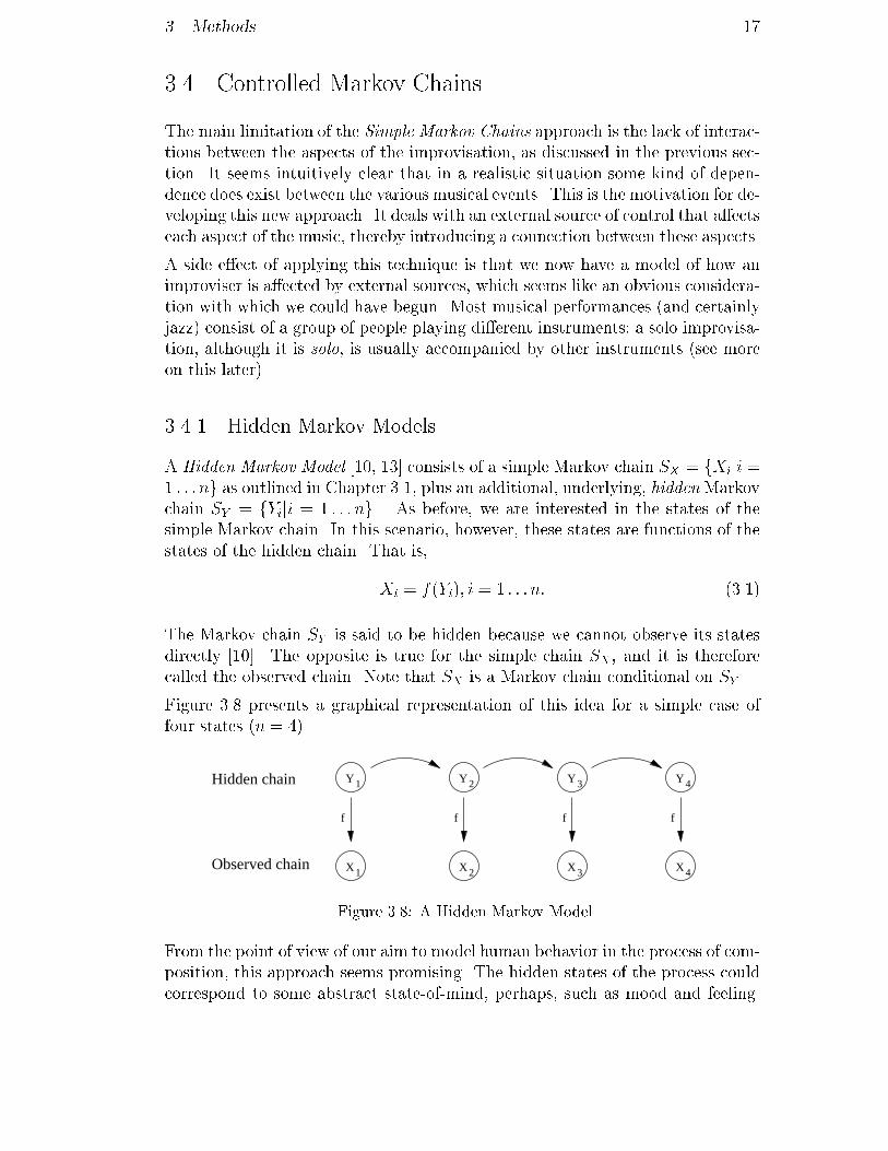
3. Methods 173.4 Controlled Markov ChainsThe main limitation of the Simple Markov Chains approach is the lack of interac-tions between the aspects of the improvisation, as discussed in the previous sec-tion. It seems intuitively clear that in a realistic situation some kind of depen-dence does exist between the various musical events. This is the motivation for de-veloping this new approach. It deals with an external source of control that a�ectseach aspect of the music, thereby introducing a connection between these aspects.A side e�ect of applying this technique is that we now have a model of how animproviser is a�ected by external sources, which seems like an obvious considera-tion with which we could have begun. Most musical performances (and certainlyjazz) consist of a group of people playing di�erent instruments; a solo improvisa-tion, although it is solo, is usually accompanied by other instruments (see moreon this later).3.4.1 Hidden Markov ModelsA Hidden Markov Model [10, 13] consists of a simple Markov chain SX = fXiji =1 : : : ng as outlined in Chapter 3.1, plus an additional, underlying, hiddenMarkovchain SY = fYiji = 1 : : : ng . As before, we are interested in the states of thesimple Markov chain. In this scenario, however, these states are functions of thestates of the hidden chain. That is,Xi = f(Yi); i = 1 : : : n: (3.1)The Markov chain SY is said to be hidden because we cannot observe its statesdirectly [10]. The opposite is true for the simple chain SX , and it is thereforecalled the observed chain. Note that SX is a Markov chain conditional on SY .Figure 3.8 presents a graphical representation of this idea for a simple case offour states (n = 4).X1 X2 X3 X4

Y 2 Y3 Y41 Y

f f f f

Hidden chain

Observed chain Figure 3.8: A Hidden Markov ModelFrom the point of view of our aim to model human behavior in the process of com-position, this approach seems promising. The hidden states of the process couldcorrespond to some abstract state-of-mind, perhaps, such as mood and feeling.

3. Methods 18The current state which the improviser is in will a�ect what he/she is playing.We can model the behavior of the improviser under each of these abstract states,and we can also model the transitions between the abstract states themselves.As encouraging as this technique may seem, we encounter a setback before wecan even try to implement it. Our general approach is to start with existing dataand then �t a model (see Section 1). However, the hidden states are not observ-able (hidden!), and so this creates a problem. We identify four possible solutions:1. Devise a di�erent approach where we do not use an existing musical piece:build the model by choosing some hidden states and \composing" the tran-sition probabilities;2. Use an existing piece, and estimate what the hidden states are;3. Use an existing piece, and assert what the hidden states are; or4. Use an existing piece and relax the restriction that the hidden states areunobservable: use some information from the music that can be observedand is believed to have an external e�ect on the improvisation.The �rst situation is a departure from our general approach (and aim). The sec-ond is the ideal solution. However, in practice it is extremely hard to estimateany information about hidden states. The third situation is also very hard toimplement, and would not guarantee an accurate model. The fourth situationseems like a worth-while simpli�cation of the technique. It can be regarded asbeing a step before the Hidden Markov Model, and hence any lessons learnedfrom it could be used in the extension to the Hidden Markov Model.The di�erence between the fourth situation and the Hidden Markov Model isthat the states of the underlying chain are not hidden. This leads to what I callControlled Markov Chains.3.4.2 Controlled Markov ChainsThe introduction of this new type of Markov chain into the model requires clar-i�cation of the terminology that will be used to distinguish it from the Markovchains we have used to this point. I will refer to the states of the chain SY asunderlying states, rather than hidden states (cf Figure 3.8), for obvious reasons;I will refer to the states of the chain SX as simple states, rather than observedstates (cf Figure 3.8) because these states are observations of the simple Markovchains discussed in the previous section. Furthermore, the word \observed" isambiguous as the underlying states are also observed.We can now estimate1. the transitions between the underlying states, and

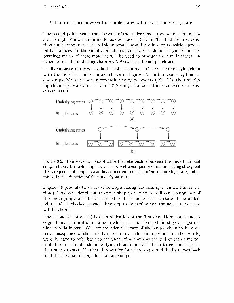
3. Methods 192. the transitions between the simple states within each underlying state.The second point means that for each of the underlying states, we develop a sep-arate simple Markov chain model as described in Section 3.3. If there are m dis-tinct underlying states, then this approach would produce m transition proba-bility matrices. In the simulation, the current state of the underlying chain de-termines which of these matrices will be used to produce the simple states. Inother words, the underling chain controls each of the simple chains.I will demonstrate the controllability of the simple chains by the underlying chainwith the aid of a small example, shown in Figure 3.9. In this example, there isone simple Markov chain, representing note/rest events (`N', `R'); the underly-ing chain has two states, `1' and `2' (examples of actual musical events are dis-cussed later).11 1 1 1

N

1 12

N

Underlying states

Simple states

Underlying states

(a)

(b)

Simple states

2 2 22

R N R R N N N N

N R N R R N N NFigure 3.9: Two ways to conceptualize the relationship between the underlying andsimple states: (a) each simple state is a direct consequence of an underlying state, and(b) a sequence of simple states is a direct consequence of an underlying state, deter-mined by the duration of that underlying state.Figure 3.9 presents two ways of conceptualizing the technique. In the �rst situa-tion (a), we consider the state of the simple chain to be a direct consequence ofthe underlying chain at each time step. In other words, the state of the under-lying chain is checked at each time step to determine how the next simple statewill be chosen.The second situation (b) is a simpli�cation of the �rst one. Here, some knowl-edge about the duration of time in which the underlying chain stays at a partic-ular state is known. We now consider the state of the simple chain to be a di-rect consequence of the underlying chain over this time period. In other words,we only have to refer back to the underlying chain at the end of each time pe-riod. In our example, the underlying chain is in state `1' for three time steps, itthen moves to state `2' where it stays for four time steps, and �nally moves backto state `1' where it stays for two time steps.

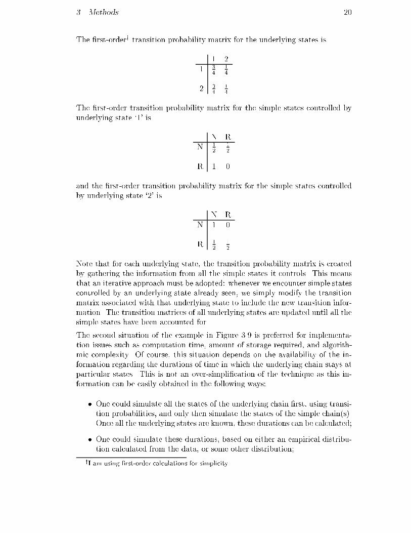
3. Methods 20The �rst-ordery transition probability matrix for the underlying states is1 21 34 142 34 14The �rst-order transition probability matrix for the simple states controlled byunderlying state `1' is N RN 12 12R 1 0and the �rst-order transition probability matrix for the simple states controlledby underlying state `2' is N RN 1 0R 12 12Note that for each underlying state, the transition probability matrix is createdby gathering the information from all the simple states it controls. This meansthat an iterative approach must be adopted: whenever we encounter simple statescontrolled by an underlying state already seen, we simply modify the transitionmatrix associated with that underlying state to include the new transition infor-mation. The transition matrices of all underlying states are updated until all thesimple states have been accounted for.The second situation of the example in Figure 3.9 is preferred for implementa-tion issues such as computation time, amount of storage required, and algorith-mic complexity. Of course, this situation depends on the availability of the in-formation regarding the durations of time in which the underlying chain stays atparticular states. This is not an over-simpli�cation of the technique as this in-formation can be easily obtained in the following ways:� One could simulate all the states of the underlying chain �rst, using transi-tion probabilities, and only then simulate the states of the simple chain(s).Once all the underlying states are known, these durations can be calculated;� One could simulate these durations, based on either an empirical distribu-tion calculated from the data, or some other distribution;yI am using �rst-order calculations for simplicity

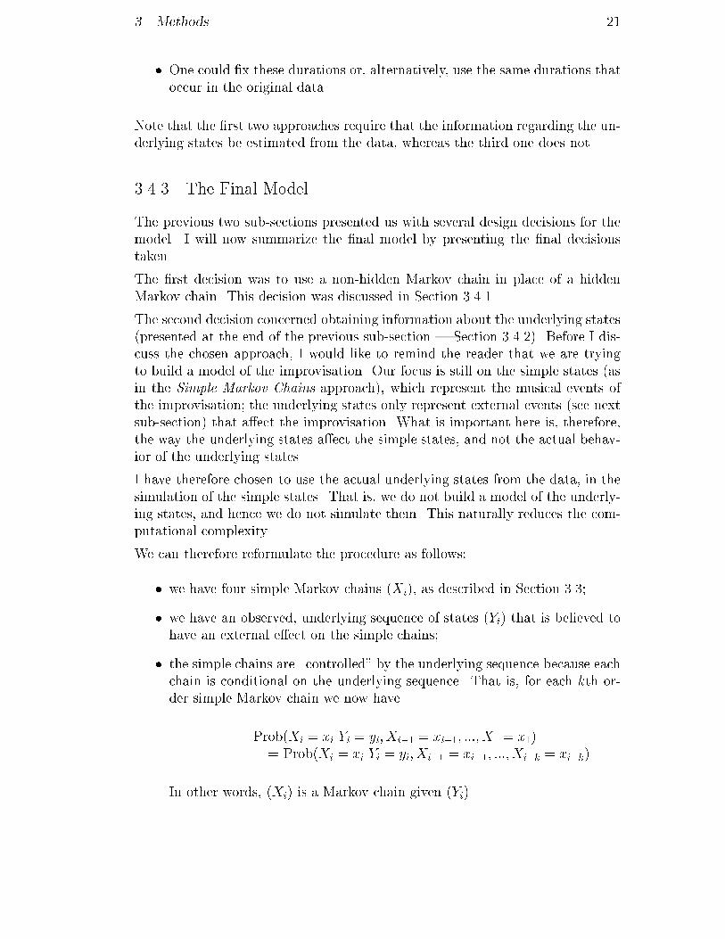
3. Methods 21� One could �x these durations or, alternatively, use the same durations thatoccur in the original data.Note that the �rst two approaches require that the information regarding the un-derlying states be estimated from the data, whereas the third one does not.3.4.3 The Final ModelThe previous two sub-sections presented us with several design decisions for themodel. I will now summarize the �nal model by presenting the �nal decisionstaken.The �rst decision was to use a non-hidden Markov chain in place of a hiddenMarkov chain. This decision was discussed in Section 3.4.1.The second decision concerned obtaining information about the underlying states(presented at the end of the previous sub-section | Section 3.4.2). Before I dis-cuss the chosen approach, I would like to remind the reader that we are tryingto build a model of the improvisation. Our focus is still on the simple states (asin the Simple Markov Chains approach), which represent the musical events ofthe improvisation; the underlying states only represent external events (see nextsub-section) that a�ect the improvisation. What is important here is, therefore,the way the underlying states a�ect the simple states, and not the actual behav-ior of the underlying states.I have therefore chosen to use the actual underlying states from the data, in thesimulation of the simple states. That is, we do not build a model of the underly-ing states, and hence we do not simulate them. This naturally reduces the com-putational complexity.We can therefore reformulate the procedure as follows:� we have four simple Markov chains (Xi), as described in Section 3.3;� we have an observed, underlying sequence of states (Yi) that is believed tohave an external e�ect on the simple chains;� the simple chains are \controlled" by the underlying sequence because eachchain is conditional on the underlying sequence. That is, for each kth or-der simple Markov chain we now haveProb(Xi = xijYi = yi; Xi�1 = xi�1; :::; X1 = x1)= Prob(Xi = xijYi = yi; Xi�1 = xi�1; :::; Xi�k = xi�k).In other words, (Xi) is a Markov chain given (Yi).

3. Methods 22The process of extracting the information from the data and building the modelis very similar to the one used with the Simple Markov Chains approach. Infact, we can even use the diagram in Figure 3.7 here. The biggest di�erence isin the middle part of the diagram | the transition probability matrices. Eachone of these is now a set of matrices, as we have seen in the example above (Sec-tion 3.4.2). The number of elements in each such set is equal to the number ofdistinct underlying states.Another di�erence (which cannot be seen in Figure 3.7) is that the extracted se-quences and simulated sequences have markers to identify where the underlyingsequence switches from one state to another. We use these markers to determinethe duration of each underlying state.The last di�erence is in the code used to perform the various tasks. This is dis-cussed at the end of this section.3.4.4 Musical ControllersA jazz improvisation is usually part of an ensemble, and so we do not have tolook far to �nd external sources that a�ect a solo improvisation. The improviseris playing a solo in the sense that the other instruments provide accompaniment;they help the improviser create the improvisation. We could probably pick anyone of these accompanying instruments to be our controlling factors. It is alsoour intuition that rhythm is a strong factor in the creation of any music.For these reasons I have decided to pick the drum track as the musical controllerfor the model. The drums form the most dominant part of the rhythm section.We want to �nd out if the drums \drive" the improvisation.In each of the examples I use, I have identi�ed distinct drum patterns whichchange the overall \mood", or \feeling", of the piece. Each of these patterns formsan underlying state in our model. In the simulation, I use exactly the same drumtrack over the simulated improvisation, as discussed in the previous sub-section.3.4.5 AlgorithmsThe function names, parallel to sep, simple, and simulate1 | used in the Sim-ple Markov Chains approach (see Figure 3.7 and Section 3.3.6), which are usedin the Controlled Markov Chains approach, are readtracks, underlying, andsimulate2, respectively.The output from MF2T is slightly di�erent in this scenario as the music is groupedinto tracks, corresponding to the underlying states. For each underlying statethere is one track, as shown in Figure B.1 | where there are three underlyingstates and hence three tracks. The values of the underlying tracks are super-imposed by the user on the second line (in the example of Figure B.1 they are

3. Methods 23\1", \2", and \1"). The C function readtracks is used to read the informationfrom these tracks. It is similar to sep but takes into the account the presence ofunderlying states, in the form of multi tracks.The S-Plus function underlying is similar to sep. It builds a separate model foreach underlying state. This function also uses transmatrix (like sep) but in addi-tion, it uses another S-Plus function editmatrix to modify a matrix correspond-ing to an underlying state that has already been seen and hence for which a matrixalready exists. This happens when an underlying state is re-visited and we use themusic under it to modify the model built when the state was previously visited.The S-Plus function simulate2 is similar to simulate1. In fact, it performs thetasks in simulate1 for each underlying state. The underlying states that appearin the original music are used here, in the simulation.The function that is used to converge all the information back into one �le is thesame as the one used by the Simple Markov Chains approach | converge.

CHAPTER 4ResultsIn Chapter 3 I presented a model and discussed its development. Two distinctparts of the development process were identi�ed and allocated separate sections,and separate model names (see Sections 3.3 and 3.4). We note that each modi�-cation of the model simply added a new feature to it, rather than created a com-pletely di�erent design. This chapter therefore deals with the statistical signi�-cance of these modi�cations, and the comparison of simulations produced by thedi�erent versions of the model, based on some pre-determined measures that arepresented in the �rst section.It is important to note that comparing single simulations is not very informative.This is due to the stochastic nature of the Markov chain. If we simulate repeadt-edly, each simulation might be completely di�erent from the one before it. Wecannot, therefore, draw conclusions based on a single simulation. A more usefulprocedure would be to simulate many times to create samples of simulations, anddraw conclusions regarding these samples. However, in some situations, compar-isons of single simulations provide a reasonable approximation to general prop-erties. In other words, in some cases we can reasonably assume that the particu-lar simulation provides a representation that is general enough for our purposes.The second and third sections deal with the contribution of each of the two ap-proaches | Simple Markov Chains and Controlled Markov Chains | to the �-nal version of the model.In the introduction (Chapter 1), I claimed that the Markov chain approach tomodeling music provides a mechanism for determining and controlling a trade-o�. This mechanism is the order of the Markov chain. It determines the extentto which the generated music copies the music being modeled (style imitation),and the extent of randomness it exhibits (spontaneous action). The �nal sectionof this chapter deals with this inherent factor that is a�ecting the model through-out its development.

24

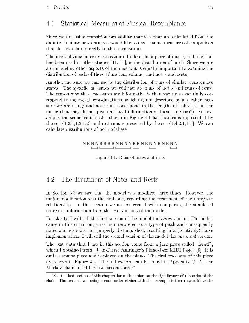
4. Results 254.1 Statistical Measures of Musical ResemblanceSince we are using transition probability matrices that are calculated from thedata to simulate new data, we would like to devise some measures of comparisonthat do not relate directly to these transitions.The most obvious measure we can use to describe a piece of music, and one thathas been used in other studies [11, 14], is the distribution of pitch. Since we arealso modeling other aspects of the music, it is equally important to examine thedistribution of each of these (duration, volume, and notes and rests).Another measure we can use is the distribution of runs of similar, consecutivestates. The speci�c measures we will use are runs of notes and runs of rests.The reason why these measures are informative is that rest runs essentially cor-respond to the overall rest-durations, which are not described by any other mea-sure we are using; and note runs correspond to the lengths of \phrases" in themusic (but they do not give any local information of these \phrases"). For ex-ample, the sequence of states shown in Figure 4.1 has note runs represented bythe set f1,2,4,1,2,1,2g and rest runs represented by the set f1,4,2,1,1,1g. We cancalculate distributions of both of these.N R N N R R R R N N N N R R N R N N R N R N NFigure 4.1: Runs of notes and rests4.2 The Treatment of Notes and RestsIn Section 3.3 we saw that the model was modi�ed three times. However, themajor modi�cation was the �rst one, regarding the treatment of the note/restrelationship. In this section we are concerned with comparing the simulatednote/rest information from the two versions of the model.For clarity, I will call the �rst version of the model the naive version. This is be-cause in this situation, a rest is interpreted as a type of pitch and consequentlynotes and rests are not properly distinguished, resulting in a (relatively) naiveimplementation. I will call the second version of the model the advanced version.The test data that I use in this section come from a jazz piece called \Israel",which I obtained from \Jean-Pierre Amringer's Piano-Jazz MIDI Page" [6]. It isquite a sparse piece and is played on the piano. The �rst two bars of this pieceare shown in Figure 4.2. The full excerpt can be found in Appendix C. All theMarkov chains used here are second-order�.�See the last section of this chapter for a discussion on the signi�cance of the order of thechain. The reason I am using second order chains with this example is that they achieve the

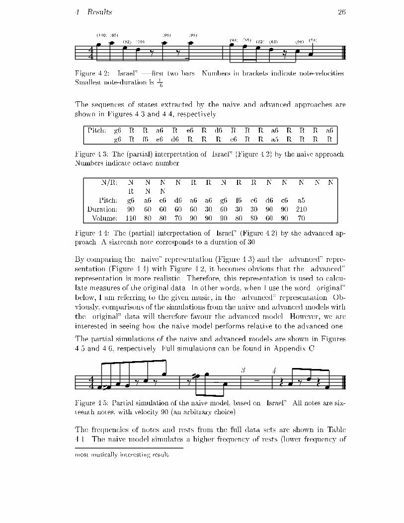
4. Results 26G 44 (110).! (85)! (82)! (79)! ? (98)! ? (98)! (93)! (85)! (82)! .(64)! @ .(98)! (73)! ..Figure 4.2: \Israel" | �rst two bars. Numbers in brackets indicate note-velocities.Smallest note-duration is 116 .The sequences of states extracted by the naive and advanced approaches areshown in Figures 4.3 and 4.4, respectively.Pitch: g6 R R a6 R e6 R d6 R R R a6 R R R a6g6 R f6 e6 d6 R R R c6 R R a5 R R R RFigure 4.3: The (partial) interpretation of \Israel" (Figure 4.2) by the naive approach.Numbers indicate octave number.N/R: N N N N R R N R R N N N N NR N NPitch: g6 a6 e6 d6 a6 a6 g6 f6 e6 d6 c6 a5Duration: 90 60 60 60 60 30 60 30 30 90 90 210Volume: 110 80 80 70 90 90 90 80 80 60 90 70Figure 4.4: The (partial) interpretation of \Israel" (Figure 4.2) by the advanced ap-proach. A sixteenth note corresponds to a duration of 30.By comparing the \naive" representation (Figure 4.3) and the \advanced" repre-sentation (Figure 4.4) with Figure 4.2, it becomes obvious that the \advanced"representation is more realistic. Therefore, this representation is used to calcu-late measures of the original data. In other words, when I use the word \original"below, I am referring to the given music, in the \advanced" representation. Ob-viously, comparisons of the simulations from the naive and advanced models withthe \original" data will therefore favour the advanced model. However, we areinterested in seeing how the naive model performs relative to the advanced one.The partial simulations of the naive and advanced models are shown in Figures4.5 and 4.6, respectively. Full simulations can be found in Appendix C.G 44 ! 4! ! ! ? ! ?��! ?4! !DD! 3 4 > ! ? ! >DD!Figure 4.5: Partial simulation of the naive model, based on \Israel". All notes are six-teenth notes, with velocity 90 (an arbitrary choice).The frequencies of notes and rests from the full data sets are shown in Table4.1. The naive model simulates a higher frequency of rests (lower frequency ofmost musically interesting result.

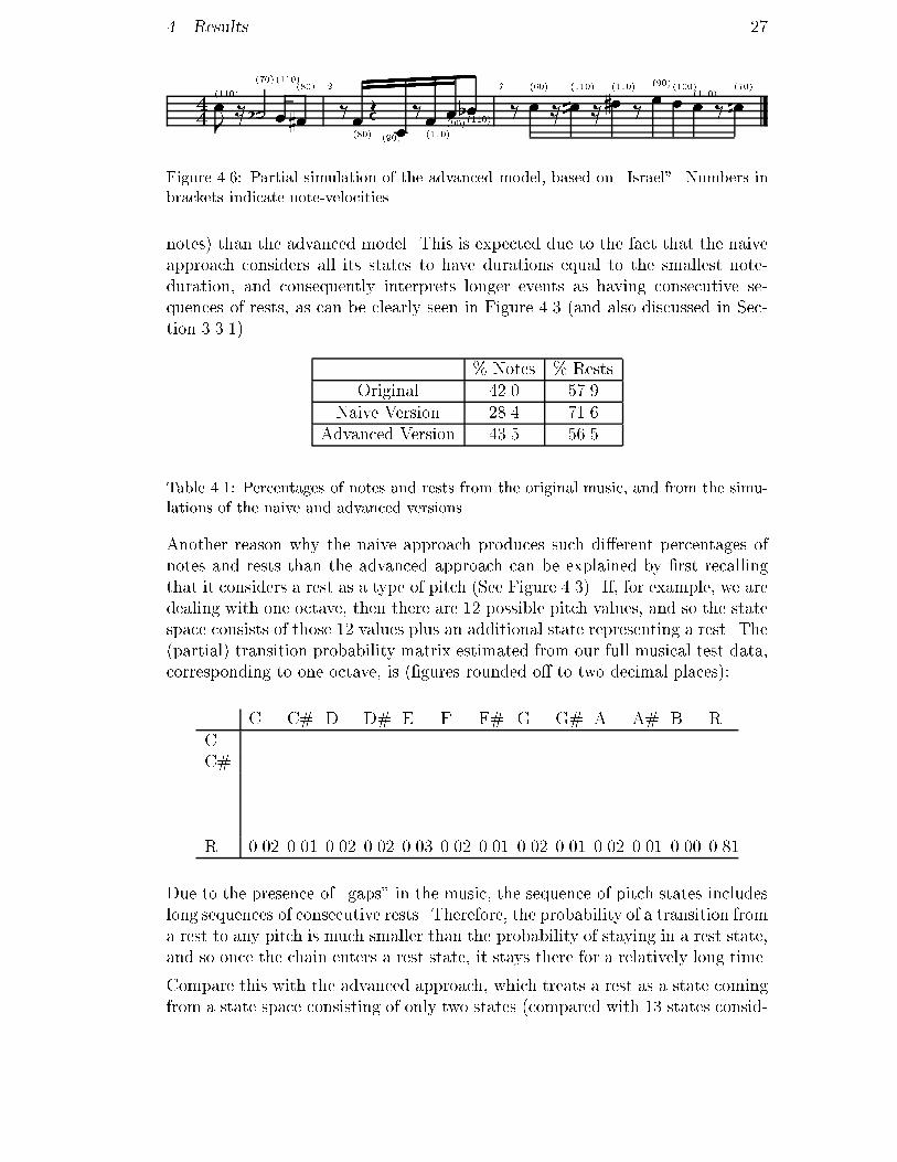
4. Results 27G 44 (110)-! @ (70)2" ..(110)! (80)4! 2? (80)! .> (90)!? (110)!��(90)!��(110)2! 3? (60)! @ (110)4! @ (110)4! .? (90)! (100)! (110)! ? (70)6!Figure 4.6: Partial simulation of the advanced model, based on \Israel". Numbers inbrackets indicate note-velocitiesnotes) than the advanced model. This is expected due to the fact that the naiveapproach considers all its states to have durations equal to the smallest note-duration, and consequently interprets longer events as having consecutive se-quences of rests, as can be clearly seen in Figure 4.3 (and also discussed in Sec-tion 3.3.1). % Notes % RestsOriginal 42.0 57.9Naive Version 28.4 71.6Advanced Version 43.5 56.5Table 4.1: Percentages of notes and rests from the original music, and from the simu-lations of the naive and advanced versions.Another reason why the naive approach produces such di�erent percentages ofnotes and rests than the advanced approach can be explained by �rst recallingthat it considers a rest as a type of pitch (See Figure 4.3). If, for example, we aredealing with one octave, then there are 12 possible pitch values, and so the statespace consists of those 12 values plus an additional state representing a rest. The(partial) transition probability matrix estimated from our full musical test data,corresponding to one octave, is (�gures rounded o� to two decimal places):C C# D D# E F F# G G# A A# B RC . .C# . .. . .. . .. . .R 0.02 0.01 0.02 0.02 0.03 0.02 0.01 0.02 0.01 0.02 0.01 0.00 0.81Due to the presence of \gaps" in the music, the sequence of pitch states includeslong sequences of consecutive rests. Therefore, the probability of a transition froma rest to any pitch is much smaller than the probability of staying in a rest state,and so once the chain enters a rest state, it stays there for a relatively long time.Compare this with the advanced approach, which treats a rest as a state comingfrom a state space consisting of only two states (compared with 13 states consid-

4. Results 28ered by the naive approach in the situation of one octave). The (partial) transi-tion probability matrix estimated for this model is:N RN ... ...R 0.36 0.64The probability of a transition from a rest to a note includes all the small prob-abilities of transitions from a rest to any pitch in the naive approach. In otherwords, the probability of leaving a rest state is now higher, producing a smallerpercentage of rests.Figures 4.7 and 4.8 present plots of the distribution of runs of notes and rests,respectively. Note that note runs here consist of any note. That is, there is nodistinction between notes with di�erent pitch, duration, and volume. Other pos-sible measures might be distributions of runs of each of these.•

•

•

• • • • • • • •

Length of Run

Fre

quen

cy

2 4 6 8 10

0.0

0.2

0.4

0.6

OriginalNaive simulationAdvanced simulation

••

••

•

•

•

•

•• • •

Figure 4.7: Plot of Note Runs.The three curves in Figure 4.7 are quite similar in shape. An interesting point tonote from this plot is that neither version simulates note runs of length greaterthan seven, which exist in the original data. In this respect, both versions arelimited in imitating the original music.The di�erences between the two versions of the model are more notable in thedistributions of rest runs (Figure 4.8). For short rest runs, of length less than

4. Results 29•

•

• ••

• • • • • • • • • • • • •

Length of Run

Fre

quen

cy

5 10 15

0.0

0.2

0.4

0.6

OriginalNaive simulationAdvanced simulation

•

•

• ••

• • ••

• • • • •

•

•

•• •

• • • • •

Figure 4.8: Plot of Rest Runs.�ve, the naive version seems to model the original data better than the advancedversion. However, for longer rest runs of length �ve to ten, the advanced versionseems to model the original data better. The advanced version does not produceany rest runs of length greater than 10, whereas the naive version produces themwith quite a high frequency, compared to the original. In fact, the accumulatedfrequencies of runs of length greater than 10, shown in Table 4.2, indicate thatthe naive version produces signi�cantly more long-runs than the advanced ver-sion and the original sequence. The explanation for this could be attributed tothe reasons discussed above. %Original 4.9Naive Version 15.2Advanced Version 2.9Table 4.2: Percentages of rest runs of length greater than 10.To summarize, we have seen that both approaches are limited, in di�erent ways,in capturing note/rest information from the original data. However, the advancedversion is clearly superior and so the extension to the Controlled Markov Chainsapproach, discussed in Chapter 3.4, is therefore based on this approach.

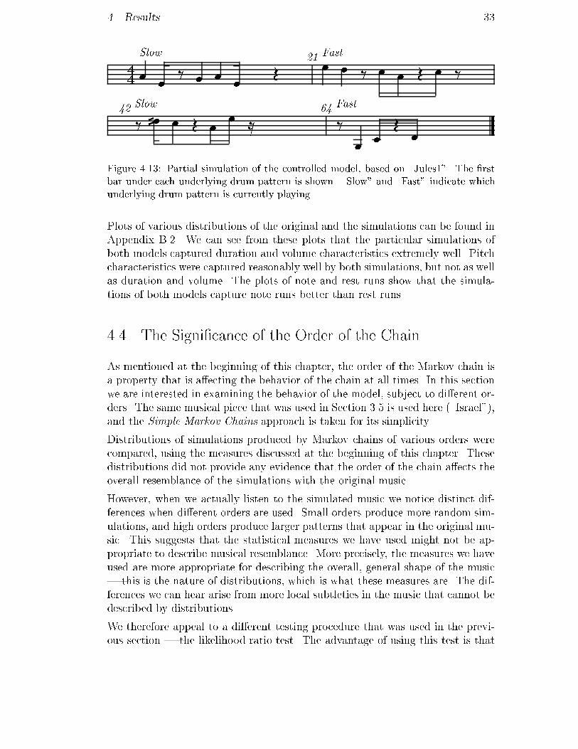
4. Results 304.3 The Signi�cance of the Underlying StatesThe modi�cation that was described in detail in Section 3.4 introduced a newlevel of control into the model. Prior to this modi�cation, the simulation of themusic depended solely on the simple Markov chains that dealt with their respec-tive aspect of the music. The purpose of this section is therefore to present someresults that might help us determine whether the addition of this new source ofdependency signi�cantly a�ects the model. In this section, I use the word \sim-ple" as shorthand for \Simple Markov Chains", and \controlled" for \ControlledMarkov Chains".As a �rst comparison between the two models, I will use a statistical techniquecalled the likelihood ratio test. Brie y, this procedure involves the following, foreach simple chain:� set the null hypothesis, H0, to be that the observed sequence is a Markovchain not dependent on the underlying states, and the alternative hypoth-esis, H1, to be that the observed sequence is a Markov chain given the un-derlying states;� calculate the likelihood of the sequence under each of H0 and H1, using thetransition probabilities of each model;� the ratio of these likelihoods has a known distribution (related to �2, un-der H0) that we can use to determine our belief in H0.For more details see Appendix A.The test data that I will use come from an improvisation played by my friend Ju-lian Bolleter. It is called \Jules 1" and is played on the piano. It is accompaniedby a drum track, which has two distinct drum patterns | a slow one and a fastone (\1" and \2", say) | that alternate twice (that is, the underlying sequence is\1" \2" \1" \2"). The drum track serves as the controlling signal. The �rst barof the music controlled by each drum pattern is shown in Figure 4.9. The full mu-sic can be found in Appendix C. As indicated by Figure 4.9 and the full excerpt,the slow drum pattern is on for 20 bars; the fast drum pattern then comes on for20 bars (bars 21 to 41); the slow drum pattern then comes back on for 21 bars(bars 42 to 63; and �nally the fast drum pattern is on for 22 bars (bars 64 to 86).The simple approach, of course, ignores information from the controlling signaland interprets the musical events as one continuous sequence. The partial mu-sical excerpt of \Jules 1", shown in Figure 4.9, is interpreted by the simple ap-proach as the sequence of states shown in Figure 4.10.The controlled approach, on the other hand, interprets sets of sequences: one foreach underlying state. This is shown in Figure 4.11, which identi�es four tracks,one for each underlying state. Note the tracks 1 and 3 are controlled by under-

4. Results 31G 44 Slow> " . 21 Fast-! ? ! ! @ ! .? 2! @G42 Slow.! ? ! @ .! 4! ! ! ? 64 Fast! ! @ ! > ! ! @Figure 4.9: \Jules1" | �rst bar under each underlying drum pattern. \Slow" and\Fast" indicate which underlying drum pattern is currently playing. See Appendix Cfor full excerpt.N/R: R R R R N . . . N R R N N RN R R R . . . N R R N R N NN N R R . . . N R N N N R RN R R R . . .Pitch: a6 . . . g6 g6 e6 g6 g#6 . . . d5 c5 d5 d#5e5 c5 . . . a5 g5 e5 g5 a5 . . .Duration: 360 . . . 60 120 30 30 30 . . . 90 60 90 3030 30 . . . 30 150 30 30 60 . . .Volume: 100 . . . 120 125 80 70 70 . . . 125 110 95 110100 110 . . . 125 85 125 90 110 . . .Figure 4.10: The interpretation of \Jules 1" (Figure 4.9) by the simple approach. Thenumber associated with a pitch indicates the octave number. Smallest note-durationis 116 , which corresponds to a duration of 30.lying state \1" (corresponding to the slow drum pattern), and so they both con-tribute to the creation of its transition probability matrix. Similarly, tracks 2 and4 are controlled by underlying state \2" (corresponding to the fast drum pattern).Our model consists of four sub-models, �tted to each of the note/rest, pitch, du-ration, and volume sequences extracted from the data. It follows that we calcu-late four likelihood values under H0, and four under H1. We perform four likeli-hood ratio tests. The p-values of the four tests for \Jules 1" are all signi�cant,suggesting that all four chains are dependent on the underlying states. In otherwords, there is signi�cant evidence from the data that the underlying states havean e�ect on each of the simple Markov chains.I will now compare simulations produced by the two models with the originaldata, using the measures discussed in Section 4.1. The simulations of the simpleand controlled models are partially shown in Figures 4.12 and 4.13, respectively.For full excerpts see Appendix C.Although the two models are statistically di�erent, it is hard to musically notice

4. Results 32N/R: 1: R R R R N . . .2: N R R N N R N R R R . . .3: N R R N R N N N N R R . . .4: N N R N R R R R N N R . . .Pitch: 1: a6 . . .2: g6 g6 e6 g6 g#6 . . .3: d5 c5 d5 d#5 e5 c5 . . .4: e5 g5 a5 e5 a5 . . .Duration: 1: 360 . . .2: 60 120 30 30 30 . . .3: 90 60 90 30 30 30 . . .4: 30 60 60 30 120 . . .Volume: 1: 100 . . .2: 120 125 80 70 70 . . .3: 125 110 95 110 100 110 . . .4: 125 85 125 90 110 . . .Figure 4.11: The interpretation of \Jules 1" (Figure 4.9) by the controlled approach.The number associated with a pitch indicates the octave number. Smallest note-duration is 116 , which corresponds to a duration of 30.G 44 Slow.! ! @ ! @DD! @ ! !

BBEEE! .? 21 Fast! > ! ? ! > ! @

G42 Slow! ? ! ! ? ! ! @ ! @ 64 Fast! ! ! ! ? ! @ ! ! .? !Figure 4.12: Partial simulation of the simple model, based on \Jules 1". The �rst barunder each underlying drum pattern is shown. \Slow" and \Fast" indicate which un-derlying drum pattern is currently playing.distinct di�erences in their simulations. The reason for this is that the durationof each underlying state (the duration of each drum pattern) is quite large. Inother words, the simple chains are controlled by each underlying state for quitea long time, and consequently the e�ect of a change from one underlying stateto the next is not very big. However, at the points where the controlling sig-nal changes its state, one does get an impression of some kind of structure beingenforced. Therefore, a more dense controlling signal (that is, changes occurringmore frequently) would have more control over the improvisation and indeed abigger musical e�ect on the listener.

4. Results 33G 44 Slow! ! ? ! ! ! > 21 Fast.! ! ? ! ! > ! ?G42 Slow.? 4! .! .> ! ! @ 64 Fast.? ! .. ! .> !Figure 4.13: Partial simulation of the controlled model, based on \Jules1". The �rstbar under each underlying drum pattern is shown. \Slow" and \Fast" indicate whichunderlying drum pattern is currently playing.Plots of various distributions of the original and the simulations can be found inAppendix B.2. We can see from these plots that the particular simulations ofboth models captured duration and volume characteristics extremely well. Pitchcharacteristics were captured reasonably well by both simulations, but not as wellas duration and volume. The plots of note and rest runs show that the simula-tions of both models capture note runs better than rest runs.4.4 The Signi�cance of the Order of the ChainAs mentioned at the beginning of this chapter, the order of the Markov chain isa property that is a�ecting the behavior of the chain at all times. In this sectionwe are interested in examining the behavior of the model, subject to di�erent or-ders. The same musical piece that was used in Section 3.5 is used here (\Israel"),and the Simple Markov Chains approach is taken for its simplicity.Distributions of simulations produced by Markov chains of various orders werecompared, using the measures discussed at the beginning of this chapter. Thesedistributions did not provide any evidence that the order of the chain a�ects theoverall resemblance of the simulations with the original music.However, when we actually listen to the simulated music we notice distinct dif-ferences when di�erent orders are used. Small orders produce more random sim-ulations, and high orders produce larger patterns that appear in the original mu-sic. This suggests that the statistical measures we have used might not be ap-propriate to describe musical resemblance. More precisely, the measures we haveused are more appropriate for describing the overall, general shape of the music| this is the nature of distributions, which is what these measures are. The dif-ferences we can hear arise from more local subtleties in the music that cannot bedescribed by distributions.We therefore appeal to a di�erent testing procedure that was used in the previ-ous section | the likelihood ratio test. The advantage of using this test is that

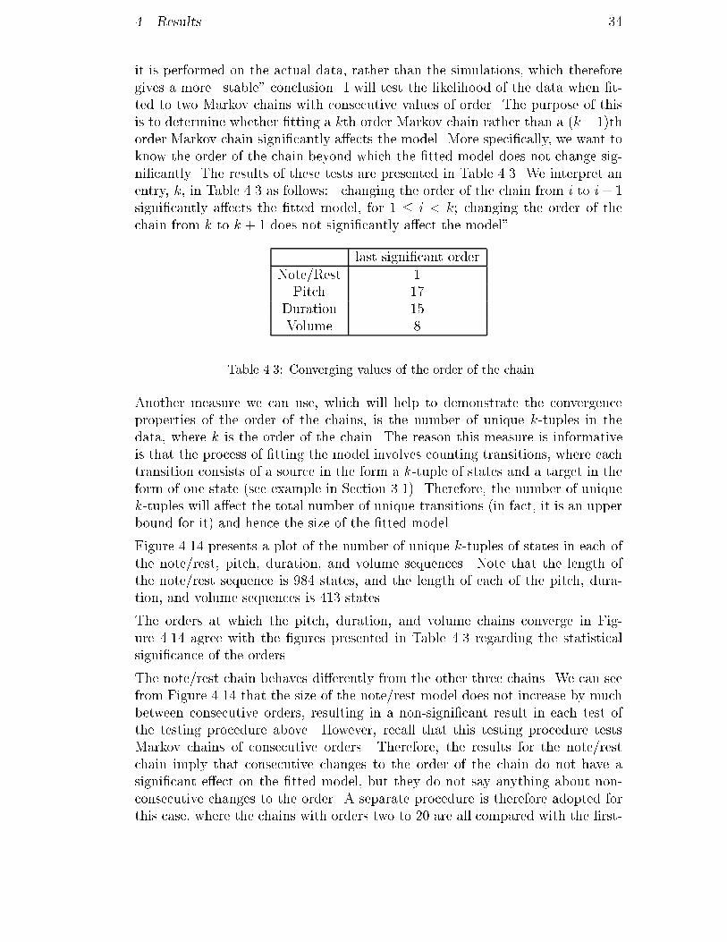
4. Results 34it is performed on the actual data, rather than the simulations, which thereforegives a more \stable" conclusion. I will test the likelihood of the data when �t-ted to two Markov chains with consecutive values of order. The purpose of thisis to determine whether �tting a kth order Markov chain rather than a (k� 1)thorder Markov chain signi�cantly a�ects the model. More speci�cally, we want toknow the order of the chain beyond which the �tted model does not change sig-ni�cantly. The results of these tests are presented in Table 4.3. We interpret anentry, k, in Table 4.3 as follows: \changing the order of the chain from i to i+ 1signi�cantly a�ects the �tted model, for 1 � i < k; changing the order of thechain from k to k + 1 does not signi�cantly a�ect the model".last signi�cant orderNote/Rest 1Pitch 17Duration 15Volume 8Table 4.3: Converging values of the order of the chainAnother measure we can use, which will help to demonstrate the convergenceproperties of the order of the chains, is the number of unique k-tuples in thedata, where k is the order of the chain. The reason this measure is informativeis that the process of �tting the model involves counting transitions, where eachtransition consists of a source in the form a k-tuple of states and a target in theform of one state (see example in Section 3.1). Therefore, the number of uniquek-tuples will a�ect the total number of unique transitions (in fact, it is an upperbound for it) and hence the size of the �tted model.Figure 4.14 presents a plot of the number of unique k-tuples of states in each ofthe note/rest, pitch, duration, and volume sequences. Note that the length ofthe note/rest sequence is 984 states, and the length of each of the pitch, dura-tion, and volume sequences is 413 states.The orders at which the pitch, duration, and volume chains converge in Fig-ure 4.14 agree with the �gures presented in Table 4.3 regarding the statisticalsigni�cance of the orders.The note/rest chain behaves di�erently from the other three chains. We can seefrom Figure 4.14 that the size of the note/rest model does not increase by muchbetween consecutive orders, resulting in a non-signi�cant result in each test ofthe testing procedure above. However, recall that this testing procedure testsMarkov chains of consecutive orders. Therefore, the results for the note/restchain imply that consecutive changes to the order of the chain do not have asigni�cant e�ect on the �tted model, but they do not say anything about non-consecutive changes to the order. A separate procedure is therefore adopted forthis case, where the chains with orders two to 20 are all compared with the �rst-

4. Results 35

• • • • • ••

•

•

•

•

••

•• • • • • •

Order

Num

ber

of U

niqu

e T

uple

s

5 10 15 20

020

040

060

080

0

•

•

•• • • • • • • • • • • • • • • • •

• ••

••

•• • • • • • • • • • • • • •

••

•

•• • • • • • • • • • • • • • • •

Note/RestPitchDurationVolume

Figure 4.14: Convergence of the number of unique tuples in the data. The length ofa tuple is equal to the order of the chain. The length of the note/rest sequence is 984states, and the length of each of the pitch, duration, and volume sequences is 413 states.order chain in hope to �nd a point where a signi�cant change occurs. However,the results of this procedure are all non-signi�cant.We can attribute the fact that the order of the note/rest chain does not a�ect its�tted model to the fact that the state space of this chain consists of only two ele-ments, compared to the other three chains whose state space consist of at least 10elements. With such a small number of states, there is not much room for varia-tions, and an order of one is high enough to capture the essence of the note/restaspect of the music.

CHAPTER 5Conclusion and DiscussionWe have seen some important developments of the model. The �rst was thetreatment of notes and rests. While this proved to be a signi�cant improvement,it also exposed the fact that this issue needs to be further developed. Our no-tion of what is a note event and what is a rest event is currently too simplistic.These events \drive" the music and so their representation needs to be complexenough to be realistic. For example, rests need to be distinguished as short rests(\breath of air"), long rests (for the purpose of \resting"), and possibly restswith durations that lie between these two. This raises the idea that durationsmust be directly associated with rest events, and it seems that notes should alsoreceive this treatment.The second development of the model was the addition of a controlling mecha-nism. This gave the music a better sense of structure, which was missing before.It also increased the applicability of the approach, putting it in the context of anensemble rather than a solo improvisation. Possibly the most important improve-ment caused by this development is the degree of dependence introduced betweenthe aspects of the music that cannot be assumed to operate independently.Although statistically the music was a�ected by the controlling signal, the de-gree of musical dependence introduced was only slight, suggesting that a moredense controlling signal (that is, more underlying states, and more frequent con-trol) might be required. Alternatively, a di�erent type of controlling signal, cor-responding to rhythm, for example, or a chord progression, could be used. Inany case, the appropriateness and applicability of this technique pave the wayfor further extensions based on this idea.We have seen that the order of the chain signi�cantly a�ects the �tted model, upto a certain converging point. This convergence is dependent on the actual sizeof the data, and the size of the state space of the various chains. A speci�c exam-ple was used to show that chains with di�erent state spaces, operating over thesame sequence, converge at di�erent points. We have also seen that any orderis generally capable of producing simulations with overall, global resemblance tothe original music. 36

5. Conclusion and Discussion 37Generally, it has been shown in this dissertation that the Markov chain techniqueis capable of capturing the global characteristics of the improvisation. A limita-tion of this project is that we have not tested local resemblances, which is statis-tically harder to do. However, as previously mentioned, when one listens to thesimulations produced by these approaches, one can de�nitely hear local patternsthat characterize the original music. Furthermore, one can hear distinct di�er-ences in the simulations when chains with di�erent orders are used.Thus one could conclude from this experiment that some kind of mathematicalstructure does exist in the process of improvisation. The Markov chain is a sim-ple mathematical model of an important aspect of human behavior: decision-making. We have seen how Markov chains can be used to model decision makinga�ected by memory alone (through the Simple Markov Chains approach), and byexternal conditions as well (through the Controlled Markov Chains approach).From a practical point of view we have developed a method, whereby we can �ta model to a given music once, and then use it to simulate repeatedly, producinga new and original piece of music each time. This is advantageous in areas thatrequire continuous music, where human intervention is undesirable, such as tele-phone hold services, restaurants, hotel lobbies, shops, elevators, etc. However,the implementation needs to be converted to real time before the techniques canbe used in these areas.The music produced by the techniques discussed in this dissertation can be cat-egorized as \pleasant". Naturally, the \human touch" is missing, but this is tobe expected in the automation of any task, by de�nition. Listeners who haveheard the results of this project have often mistaken the simulated music for the\real" music. The techniques have been successful at capturing and reproducingthe musical elements that make a jazz improvisation exciting and unpredictable.

References1. Commonmusic. An object oriented music composition environment imple-mented in Common Lisp. Runs on NeXT, Macintosh, SGI, SUN, and I386.http://www.eecs.umich.edu/ mrozek/nextmusic/CommonMusic.html.2. Keykit. A programming language and graphical user interface for MIDI.Runs on Windows 95 and Linux. http://www.nosuch.com/keykit.3. S-Plus. A statistical, data-analysis, programming language.http://www.mathsoft.com/splus.4. Charles Ames. Automated composition in retrospect: 1956{1986. Leonardo,20(2):169{185, 1987.5. Charles Ames. The Markov process as a compositional model: A survey andtutorial. Leonardo, 22(2):175{187, 1989.6. Jean-Pierre Amringer. Jean-Pierre Amringer's piano-jazzMIDI page. Available through the World Wide Web at:http://www.worldnet.fr/ jpa/midi.shtml.7. Adrian Baddeley. Babble, 1988. A program that �ts a Markov chainto words or characters in a text �le, and simulates new text. E-mail:[email protected]. Derek Bailey. Improvisation. Its Nature and Practice in Music. Derek Bai-ley, 1980.9. R.A. Becker, J.M. Chambers, and A.R. Wilks. The NEW S Language. 1988.10. Robert J. Elliott, Lakhdar Aggoun, and John B. Moore. Hidden MarkovModels. Estimation and Control. Springer-Verlag New York, Inc., New York,1995.11. Topi Jarvinen. Tonal hierarchies in jazz improvisation. Music Perception,12(4):415{437, 1995. 38

References 3912. Kevin Jones. Compositional applications of stochastic processes. ComputerMusic Journal, 5(2):381{397, 1981.13. David H. Kil and Frances B. Shin. Hidden markov models. In Pattern Recog-nition and Prediction With Applications To Signal Characterization, chap-ter 5, pages 155{86. American Institute of Physics Press, New York, 1996.14. C. L. Kruhhansl. Cognitive Foundation of Musical Pitch. Oxford UniversityPress, New York, 1990.15. Emanuel Parzen. Stochastic Processes. Holden-Day, Inc., San Francisco,1962.16. Je� Pressing. Cognitive processes in improvisation. In W. R. Crozier andA. J. Chapman, editors, Cognitive Processes in the Perception of Art, pages345{63. Elsevier Science Publishers B.V., Amsterdam, 1984.17. Je� Pressing. Improvisation: Methods and models. In John A. Sloboda, ed-itor, Generative Processes in Music: The Psychology of Performance, Im-provisation and Composition, chapter 7, pages 129{78. Oxford UniversityPress, New York, 1988.18. Piet van Oostrum. MF2T for Unix. Dept. of Computer Science, UtrechtUniversity. P.O. Box 80.089, 2508 TB Utrecht, The Netherlands. email:[email protected]. A C-program for converting MIDI �les to text �les.19. Iannis Xenakis. Formalised Music. Indiana University Press, Bloomington,Ind, 1971.

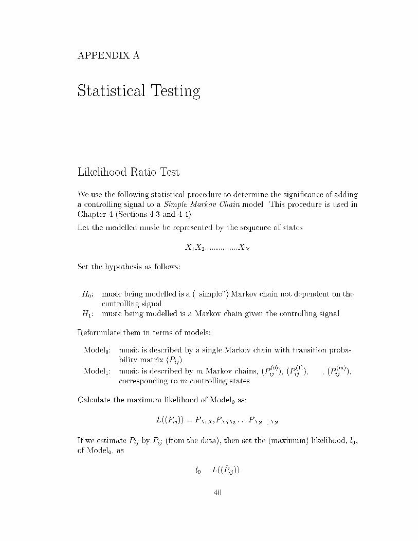
APPENDIX AStatistical TestingLikelihood Ratio TestWe use the following statistical procedure to determine the signi�cance of addinga controlling signal to a Simple Markov Chain model. This procedure is used inChapter 4 (Sections 4.3 and 4.4).Let the modelled music be represented by the sequence of statesX1X2:::::::::::::::XNSet the hypothesis as follows:H0: music being modelled is a (\simple") Markov chain not dependent on thecontrolling signalH1: music being modelled is a Markov chain given the controlling signalReformulate them in terms of models:Model0: music is described by a single Markov chain with transition proba-bility matrix (Pij)Model1: music is described by m Markov chains, (P (0)ij ), (P (1)ij ), . . . , (P (m)ij ),corresponding to m controlling states.Calculate the maximum likelihood of Model0 as:L((Pij)) = PX1X2PX2X3 : : : PXN�1XNIf we estimate Pij by P̂ij (from the data), then set the (maximum) likelihood, l0,of Model0, as l0 = L((P̂ij))40

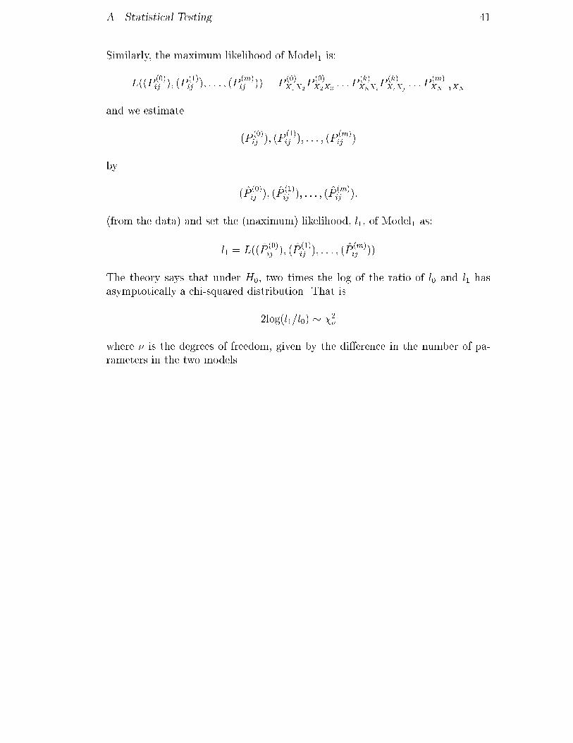
A. Statistical Testing 41Similarly, the maximum likelihood of Model1 is:L((P (0)ij ); (P (1)ij ); : : : ; (P (m)ij )) = P (0)X1X2P (0)X2X3 : : : P (k)XhXiP (k)XiXj : : : P (m)XN�1XNand we estimate (P (0)ij ); (P (1)ij ); : : : ; (P (m)ij )by (P̂ (0)ij ); (P̂ (1)ij ); : : : ; (P̂ (m)ij ):(from the data) and set the (maximum) likelihood, l1, of Model1 as:l1 = L((P̂ (0)ij ); (P̂ (1)ij ); : : : ; (P̂ (m)ij ))The theory says that under H0, two times the log of the ratio of l0 and l1 hasasymptotically a chi-squared distribution. That is2log(l1=l0) � �2�where � is the degrees of freedom, given by the di�erence in the number of pa-rameters in the two models.

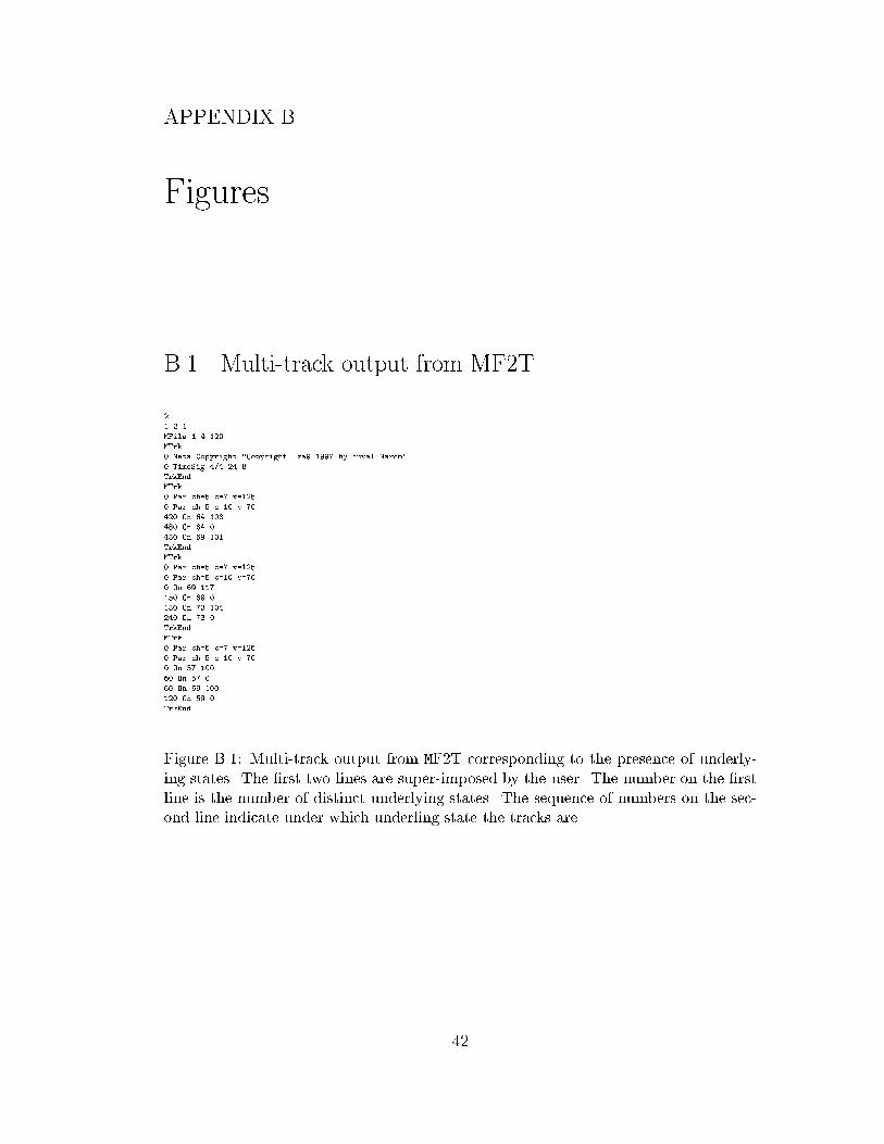
APPENDIX BFiguresB.1 Multi-track output from MF2T21 2 1MFile 1 4 120MTrk0 Meta Copyright "Copyright \xa9 1997 by Yuval Marom"0 TimeSig 4/4 24 8TrkEndMTrk0 Par ch=5 c=7 v=1250 Par ch=5 c=10 v=70420 On 64 108480 On 64 0480 On 69 101TrkEndMTrk0 Par ch=5 c=7 v=1250 Par ch=5 c=10 v=700 On 69 117150 On 69 0180 On 73 104240 On 73 0TrkEndMTrk0 Par ch=5 c=7 v=1250 Par ch=5 c=10 v=700 On 57 10060 On 57 060 On 59 100120 On 59 0TrkEndFigure B.1: Multi-track output from MF2T corresponding to the presence of underly-ing states. The �rst two lines are super-imposed by the user. The number on the �rstline is the number of distinct underlying states. The sequence of numbers on the sec-ond line indicate under which underling state the tracks are.

42

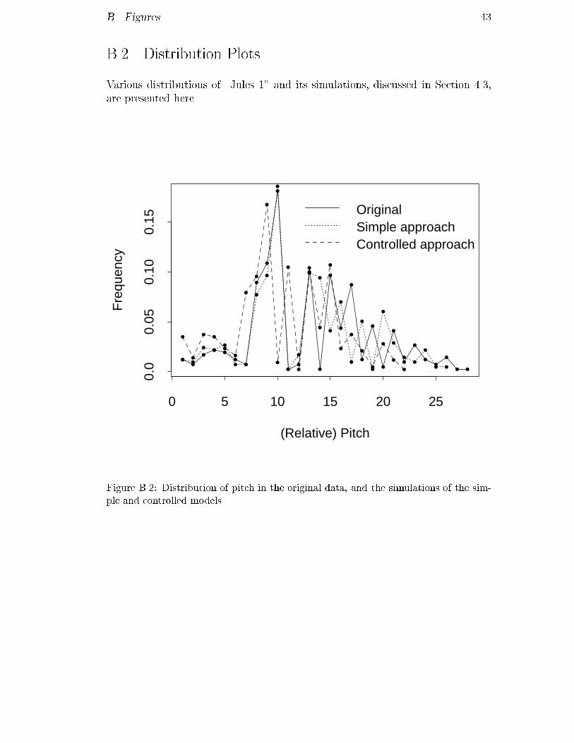
B. Figures 43B.2 Distribution PlotsVarious distributions of \Jules 1" and its simulations, discussed in Section 4.3,are presented here.

• •• • • • •

•

•

•

• •

•

•

•

•

•

•

•

•

•

••

• • •• •

(Relative) Pitch

Fre

quen

cy

0 5 10 15 20 25

0.0

0.05

0.10

0.15

• •• • •

• •

•

•

•

••

• •

•

•

•

•

•

•

•• •

•• •

•

•

• •• •

••

•

•

•

•

•

•

•

••

••

••

•

OriginalSimple approachControlled approach

Figure B.2: Distribution of pitch in the original data, and the simulations of the sim-ple and controlled models

B. Figures 44•

•

••

•

Duration

Fre

quen

cy

40 60 80 100 120 140

0.0

0.2

0.4

0.6

•

•

•

••

•

•

•

• •

OriginalSimple approachControlled approach

Figure B.3: Distribution of duration in the original data, and the simulations of thesimple and controlled models. A quarter note has duration 30

• • • • ••

•• • • • • •

••

•

•

(Relative) Volume

Fre

quen

cy

5 10 15

0.0

0.1

0.2

0.3

0.4

• • • • • ••

• • • • • •

•

•

•

•

• • • • • • • • • • ••

•

•

•

•

•

OriginalSimple approachControlled approach

Figure B.4: Distribution of volume in the original data, and the simulations of the sim-ple and controlled models

B. Figures 45•

•

•

• • •

Length of Run

Fre

quen

cy

1 2 3 4 5 6

0.0

0.2

0.4

0.6

•

•• •

•

• •

OriginalSimple approachControlled approach

Figure B.5: Distribution of note runs in the original data, and the simulations of thesimple and controlled models•

• •

•

• •• • •

Length of Run

Fre

quen

cy

2 4 6 8

0.0

0.1

0.2

0.3

•

•

•

•

••

•• •

••

•

•• •

• • •

OriginalSimple approachControlled approach

Figure B.6: Distribution of rest runs in the original data, and the simulations of thesimple and controlled models

APPENDIX CMusical ExcerptsThe full musical excerpts of all the examples and simulations used in this disser-tation are presented in the following pages.

46

C. Musical Excerpts 47IsraelG 44 .! ! ! ! ? ! ? ! 2 ! ! ! .! @ .! ! ..zG 3{! ..> ! @ 4! ! !z 4{! . .. 5 .> ! 4! @ ! ? 6!G 6 ? ! ! @ ! @ ! @ ! ..z 7{ @@@! .> ! ! @EE .! @G 8 )!z 9{! @ ! ! @ ! 2! ? 4!z 10{4! .! ����2!zG11{2! @ 6!DD! @ !EEE .! @ ! .! 12 -! @ !G13 .! ! ! ! ? ! @ ! @ 14 ! ! ! @ ! ? ! @ ! ..zG15{! ..> ! @ 4! ! @ .!z 16{! . .. 17 .> ! 4! .! ? 6!G18 ? ! ! .! @ ! @ ! ..z 19{ @@@! ..> ! @ @@@EE! ? .! @G20 @ @@@! ..> ! ! ..>DDEE!z 21{! .! ! @ ! 2! ? 4!zG22{4! ! @ ����2!z 23{2! 6! @DD! ! @EEE! @ ! -! 24 -! @ ! . .>G25 ! ! ! ! 2! 6! ! @ ! ..> 26 .? ! ! ! @ 2! 6! ? !G27 ..> ! ! @ ! ..> 28 @ ! 2! 4! @ 2! 6! 2! @ ! @ 6!G29 @ )! 30 ! @ 4! 4! ? ! !z 31{! 4! ? 6! @ ! .>

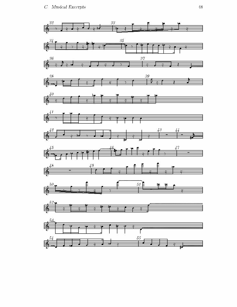
C. Musical Excerpts 48G32 .? ! @ ! @ ! ! @ 2! ..z 33{ .2! > ! @ ! @��6! @���2! @G34 ! @ ! .? ! @ 4! 6! @ 4!z 35{4! ? ! 4! ! ! ! 6! @ ! .! @G36 @ )! @ 2! @ ! ! @ ! ? ! 37 @ ! @ ! ..> ! ..zG38{! 4! ! ! @ ! ! @ ! ? ! 39 -! @ ! .. .> )!G40 @ ! ! ! @ 2! 6! @ 2! @ 4! @ 2! 6!G41 .? ! 2! ! @ ! ! @ 2! 6! ! !G42 ! ! @ 2! ? ! 2! ! @ 4! @ 6! @ 43 44 4 )!zG45{4! ! ! 2! .! 4! 4! ! !z 46{4! ! ! 2! ! @ ! ! ! ? 47G48 49 ! ! ! @ ! ! ! @ ! @ 2! @G502! ? ! ? ! @EEEEE! ? ! ..z 51{! 4! 6! ! @G522! @ 4! @ 6! @ 4! 6! @ ! ! @ !zG53{! ! 2! ! 2! @ 6! ! 6! 2! @ !zG54{! ! 4! ! ! @ ! 2! @ 55 .! ! .! ! @ 4! ..z

C. Musical Excerpts 49G56{4! . @ ! @ ! @ .4!z 57{ .4! 6! ? 58 .? ! ..> !zG59{ .! > ! @ ! @ 60 4! @ 4! 6! 2! @ ! @ 4! ! @ ! !zG61{! ! ! ! ! @ ! .> 62 ..> ! ! ! ! ! 2! ! ! ! @ !zG63{" ... .> 642! @ ! 4! 4! ! @ 2! @ ! 6!z 65{! ! @ ! .. .>G66 .? 4! ! ! 2! ! 4! 4! !z 67{ @@@! @ ! @ .! >EEE2! ?G68 4! ! @ 6! @ 4! @ ! @ 2! ! 4!z 69{4! @ ! .! ..> .6! @G70 ! @DD .! .> !z 71{ .! > ! .! ! @ ! !G72 ! ! ! @ ! @ ! @ ! ? 73 . !zG74{! ? ! .? ! 2! 2! ! 4! ! !z 752!{2! @ ! 4!����! . 76G77 @ ! @ 4! 6! @2! @ ! ! @ 4! @ 4! 78 @ ! @2! @ ! ! @ 4! @ 4! @ 6! !zG79{! ! ! .! ! 2! ! ! ! ! ! 80 .! 2! ! @ ! ! ! ! .? ! 4!G81 4! ! @ 4! ! ! 2! ! 4! ! ! ! @ ! 82 ! 2! ! ! ! @ ! @ 4! @ 6! ?G83 4! ? ! 4! ! ! ! 6! @ ! .2! @ 84 @ ! @ ! ? ! ? ! ? !

C. Musical Excerpts 50\Naive" Simulation of Israelby Yuval Marom and S-PlusG 44 ! 4! ! ! ? ! ?��! 2 ? 4! !DD! 3 4 > ! ? ! >DD!G 54! ! ! ! ? 4! ! ! 6 4! ! ! ! 7 . -! ? 8 -! 9 ? 4! ? !G10 11 4-! 12 ! > ! 4!DD4! > 13 . -! ? 14 15 ? ! ..!G16 -! .> 17 > ! > ! ? ! 18 ? ! > 2! !��4! ? 19 ! > ! ! 2! 6! !G20 ? ! ? ! ? 2!EE! ? 21 ? 2! 6! ? ! ? ! ? 22 ! ? 2! 6! >��! ?G23 ! ! ? ! 24 ? ! ?��! 25 (! .> 26 ..4! 6! 2! 27 ? 2! ?CC!G282! ! > 29 (! 30 ! ? ! ? 31 32 ? ! ..��! 33 > ! >! >G34 ! 2! ! ! ! .> 35 36 ? -! . 37 .. 4 (! > 38 > ! .>��! ?G39 ! ! ? 2! .>EE! 402! ? 6! ? ! ? 2! ! 41 4! .> ! .> 42 43 .. -! >G44 ..! ? 4! 45 .. (! > 46 47 -! .> 48 49 .> -! 50 ? ! ..II!G51 (! 52 > (! .. 53 ? ! ..UU! 54 ..! ! ? 55 56 -!G57 ? 2! 6! ? ! >EE! 582! ? 6! ? 2! ? ! ! 59 ! ? ! 2! ! ? ! ?G60 ? 2! 2! ! 4! ? ! ! 61 4! ? 6! 4! .> ! 62 ? -! . 63 .> (!

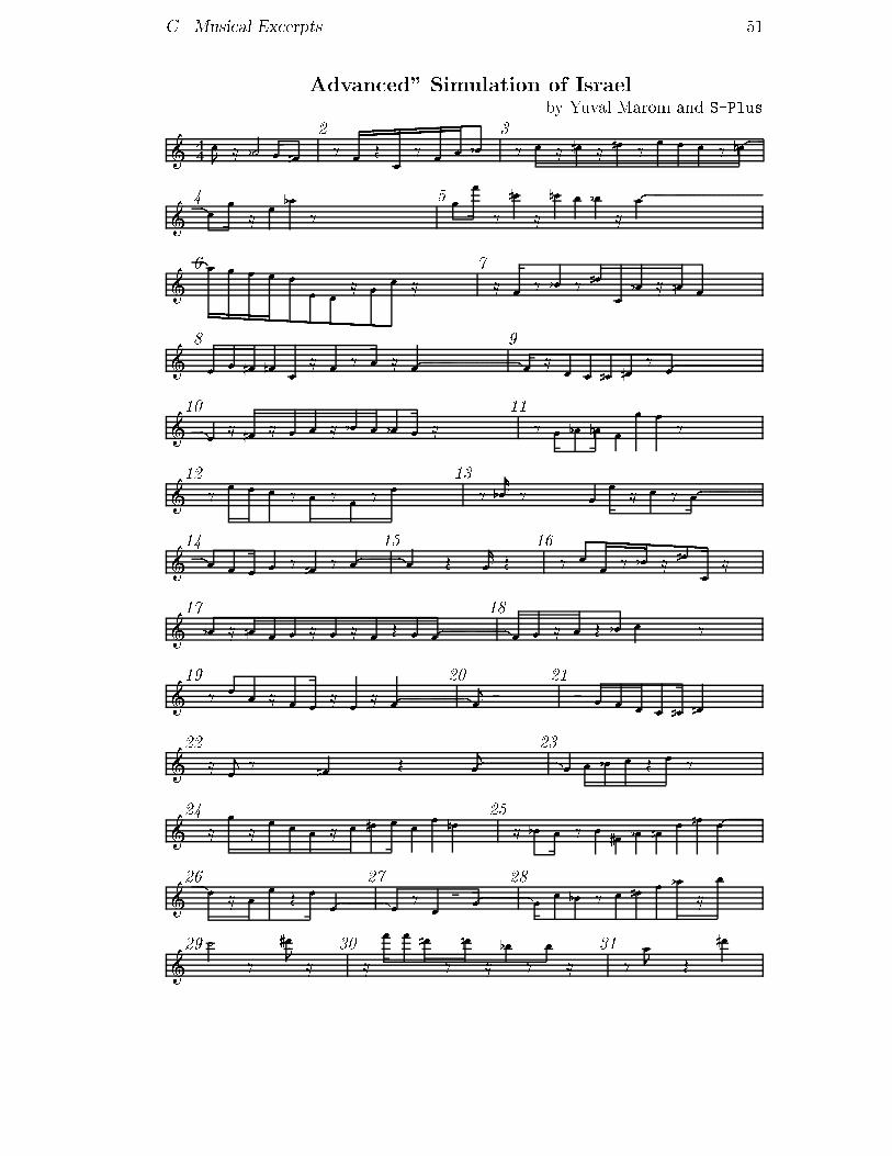
C. Musical Excerpts 51\Advanced" Simulation of Israelby Yuval Marom and S-PlusG 44 -! @ 2" .. ! 4! 2 ? ! .> ! ? !��!��2! 3 ? ! @ 4! @ 4! .? ! ! ! ? 6!zG 4{ .! ! @ ! .2! ? 5 .! ! ? 4! @ 6! ! 2! @ !zG 6{! ! !DD! ! ! ! @ !EEE! @ 7 @ ! .? 2! ? 4! ! 2! @ 6! !G 8 ! ! 4! 6! ! @ ! ? ! @ !z 9{! @ .! ! 4! 4! ? .!zG10{! @ 4! @ ! ! @ 2! ! 2! ! @ 11 .? ! 2! 6! .! ! ! .?G12 ? ! ! ! ? ! .? ! ? ! 13 ? 2 )! ? ! ! @ ! ? !zG14{! ! ! .! .? 4! ? !z 15{! .. > )! .> 16 .? .! ! .?CC2! @ 4! AAEE! @G172! @ 6! ! ! @ ! @ ! > ! !z 18{! ! @ ! > 2! ! ?G19 .? ! ! @ ! ! @ ! @ !z 20{ (! . . 21 ! ! ! ! 4! 4!G22 @ (! ? 4! ..> (!z 23{! .. ! 2! ! ..> ! ?G24 @ ! @ ! ! ! @ ! 4! ! ! ! 6! 25 @ 2! ! ? ! 4! 2! 6! ! 6! !zG26{! @ ! ! > ! ! .z 27{! ? ! !z 28{! ! 2! ? ! 4! ! 2! @ !G29 " .. .? 4 -! @ 30 @ ! ! 4! ? 6! @ 2! ? ! @ 31 .? -! ..> 4! .

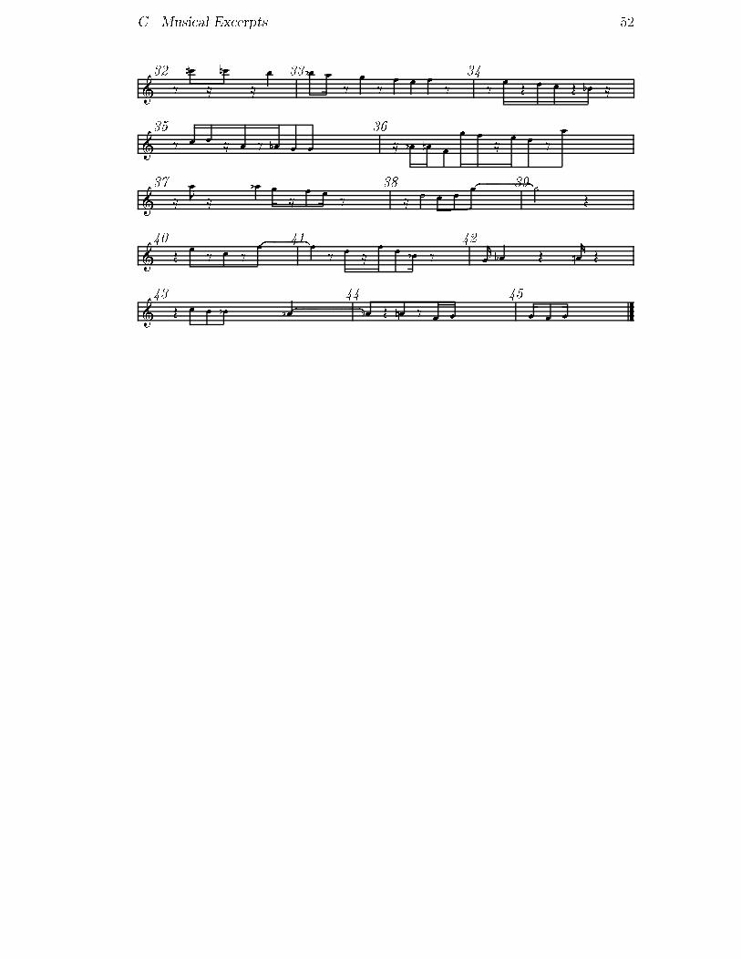
C. Musical Excerpts 52G32 .? 4! @ 6! @ ! . 332! ! .? ! ? ! ! ! ? 34 .? ! > ! ! > 2! @G35 .? ! ! @ ! .? 2! ! .! 36 @ 2! 6! ! ! ! @ ! ! .? !G37 @ -! @ 2! .. ! @ ! ! ? 38 @ " .! !��!z 39{" ... .>G40 > ! .? ! .? !z 41{! ..? ! @ ! ! 2! .? 42 )! 2! ..> 6 )! ..>G43 .> ! ! 2! 2!z 44{ .2! .> 6! ? ! ! 45 ! ! !

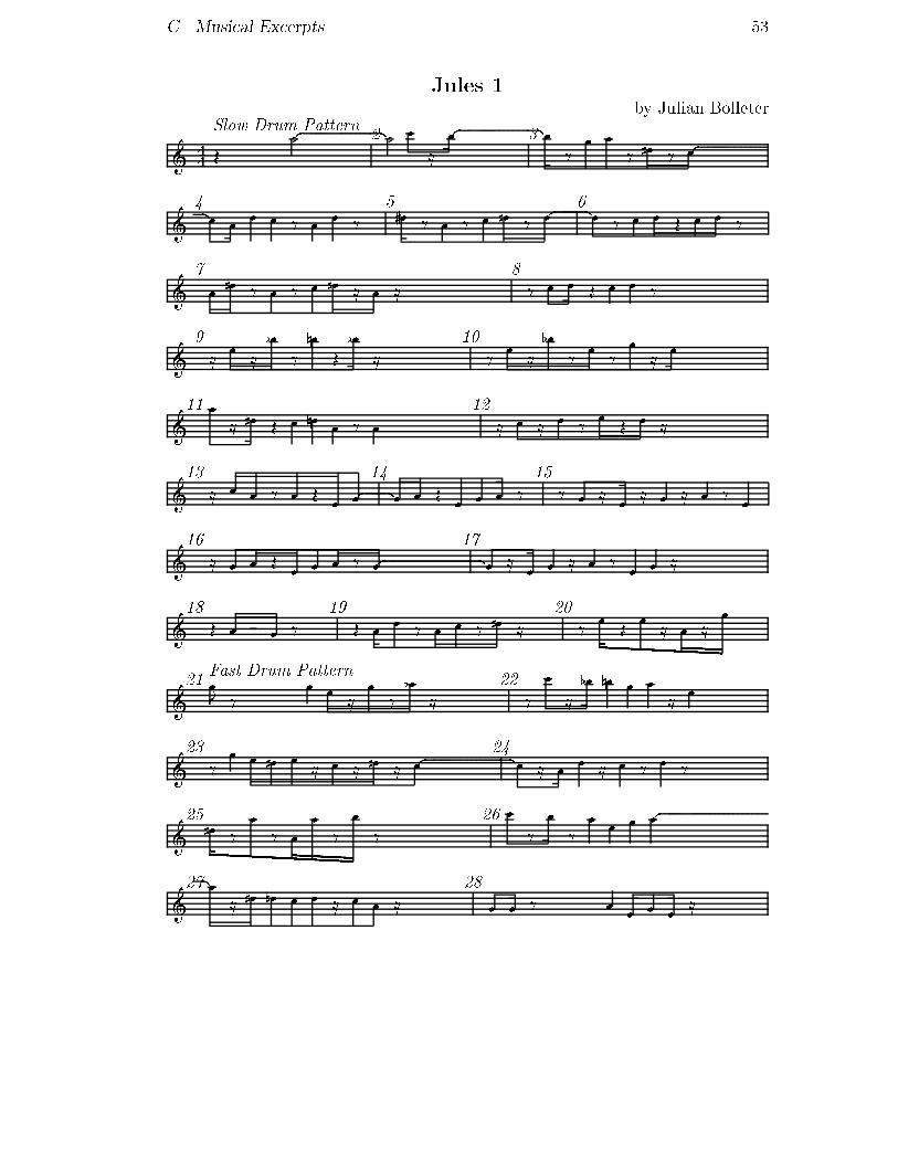
C. Musical Excerpts 53Jules 1 by Julian BolleterG 44 Slow Drum Pattern> " .z 2{" . ! @ !z 3{! .? .! ! .? 4! ? !zG 4{ .! ! .! ! ? ! ! ? 5 4! .? ! ? .! 6! .? !z 6{! .? ! ! > ! ! ?G 7 ! 4! .? ! ? .! 6! @ ! @ 8 ? ! ! ..> .! ! ?G 9 @ ! @ 2! .? 6! ..> 2! @ 10 ? ! @ 2! ? ! .? .! @ !G11 ! @ 4! ..> ! 6! ! ? ! 12 @ ! @ .! ? ! > ! @G13 @ ! ! ? ! .> ! !z 14{! ! .> ! ! ! ? 15 ? .! @ ! @ ! @ ! .? !G16 @ ! ! > ! ! ! .? !z 17{ .! @ ! ! @ ! .? ! ! @G18 > ! ! ? 19 > ! ! ? ! ! .? 4! @ 20 ? @@@! .> .! @ ! @CCEE!G21 Fast Drum Pattern-! ? ! ! @ ! .? 2! @ 22 .? ! @ 2! .6! ! ! @ !G23 ? ! ! 4! ! @ ! @ 6! @ !z 24{! @ ! ! @ ! .? ! .?G25 @@@4! ? ! ? ! ! .?DDEE! .? 26 ! ? ! ? .! ! .! !zG27{! @ 4! 6! ! ! @ .! ! @ 28 ! ! .? ! ! .! ! @

C. Musical Excerpts 54G29 .? ! .? ! @ ! > !z 30{! @ ! .? ! @ 2! ? ! @G31 .? ! ? ! @ ! >CCEE!z 32{! @ ! .? ! ..2! 6! ! @G33 .? ! @ ! .? ! ! ! ? 34 ? ! ! @ ! @ 4! ? ! ! @ 6! @G35 ? ! .! @ ! ? ! ? !z 36{! ? ! @ ! ! ! @ ! ! ?G37 .? ! .? ! ..> !z 38{ )! ..> ! ! ! ? ! @ 39 .? ! ? .! @ ! ? !zG40{! @ ! .? 2! .? ! ! @ ! 41 .? .! ! 4! ! @ ! 6! @ !zG42 Slow Drum Pattern{ .! ? ! @ .! 4! ! ! ? 43 ! .. )! ? ! @ ! !G44 ! . !����! ? 45 @ ! ! .? .! ! .? 46 4! > .! @ .! 6! .?G47 @ .! @ .! @ ! ? ! ? 48 @ ! ! @ ! .? ! > ! @G49 ! .! @ 4! 6! ? ! ? ! .? 50 @ .! ! .? .! ? ! !G51 ? ! ? ! .? ! ! @ ! @ 52 ! .> .! .? ! 53 ? ! @ ! ..> ! .? !zG54{! ? ! @ ! > .! ! @ !z 55{! @ ! .? ! ! ? ! .? !G56 ! @ ! ..>��! .?�� .! 57 @@@!BB! @ ! ! ! ! ? ! @

C. Musical Excerpts 55G58 @ 4! 4! @ 6! @ 6! ! .> 4! 59 .? ! ? ! ? ! @ ! @ !G60 .? ! @ ! @ 4! ? ! @ ! @ 61 @ ! ! .! .4! ? ! !zG62{4! @ ! 4! ! ? ! .? ! @ ! @ 63 )! @ ! .. ! ! ? ! .?G64 Fast Drum Pattern! ! @ ! > ! ! @ 65 ! > ! .> .! 66 @ ! ! @ ! ! .? ! .? !G67 @ ! ! @ ! ! ? ! .? ! ! @ 68 .? ! .? ! ?��! .?��!G69 .! @ ! @ AADD! ! ? ! .? 70 @ ! .> .! .? ! @ 71 ..> ! > ! ! .?����!G72 ? ! @ 4! .? ! @ ! .! @ 73 @ .! @ ! @ ! ..> ! @G74 ! > ! @ ! @ ! @ ! ? 75 .? ! .> ! .?DDDD! @ 76 ! @ ! > ! ? ! ?G77 @ ! @ ! ! @ ! ? ! @ ! 78 ! @ ! ? ! ? 4! @ ! ! @G794! ! ? ! ? 6! @ ! ! @ 80 @ .! @ ! ! ! @ ! ! @ ! @G81 @ ! @ ! ! .? .! @ ! !z 82{! @ ! .? ! ! @ ! .? !G83 @ ! ! > ! .? ! 84 ! ! ? ! .? .! ? ! @G85 ? ! .? ! .? ! .? 4! 6!z 86{! !CCCC! ? ! )!

C. Musical Excerpts 56\Simple" Simulation of Jules 1by Yuval Marom and S-PlusG 44 Slow Drum Pattern.! ! @ ! @DD! @ ! !BBEEE! .? 2 ! ! 2! > ! @ ! ? ! @G 3 ! .? ! @ 2! @ ! .? ! 4 .? ! .? ! .! !z 5{ @@@! @ ! ..> @@@DD! > !G 6 @ -! ! @ @@@! @CC .2! .? 7 ! @ ! ! @ ! @ 4! 6! .? ! @G 8 ! @ 4! @ ! ! 6! ? ! @ ! @ 9 .> ! .?CC! .?DD4!G10 ? AA! ! .> ! @ AAEE! @ 11 @ AA!BB! . 12 @ ! ! ! .? ! ? ! @G13 .? @@@! ? ! ? @@@DD! ! ? ! 14 @ ! @CCCC! ? ! ! ? ! @G15 ! ! ? ! ! ? .! ? 16 ! @ 4! ! ! @EE! .>EE6!zG17{! ! @ ! .? ! ? ! ? ! 18 ! @ ! @ ! > 4! ? ! !zG19{ .! ! .> ! > 4! 20 @ ! > ! @ .4! .? 21 Fast Drum Pattern! > ! ? ! > ! @G22 ? .! ? ! ? ! @ ! @ ! 23 GG! ?II! ! @ ! @ .! @G24 ? ! .! ! @ .! ! ? ! @ 25 ! .> .! @ ! @ !z 26{! ? ! > ! ! !G27 .? ! ..? ! .! @ 28 ? ! @ ! @ ! ? ! ! .? ! !z

C. Musical Excerpts 57G29{! @ ! ! ! ! ! > .! 30 .> ! ! ..> !zG31{@@@! ! @ @@@DD! .! ? ! .? ! 32 .! .? ! ? ! .! ! !zG33{! @ ! ? ! ? ! ? 4! .!z 34{! @ ! ..> ! ! ! @ !zG35{ .! ? ! .! ? ! .? ! 36 ? .! ? ! @ ! ! @ ! !zG37{! ? ! @ ! ! @ ! ? ! ! @ 38 ! > ! @ ! .? .!G39 .4! @ ! @ ! 6! ! > ! ! !z 40{! @ ! @ ! ! @ ! ! ! @ ! ! @G41 ! ! ! > ! .! @ ! 42 Slow Drum Pattern! ? ! ! ? ! ! @ ! @G43 @ .! ? ! @ ! .? ! .! 44 ! ? ! @ ! @ ! ? 2! @ !zG45{! @ ! ? ! ! ? ! ! @ !z 46{ .! ? ! ! .! ? ! @ ! !G47 ? ! ? ! ..> ! ? 4!z 48{4! @ ! ! ? ! 49 ? ! @ ! ? ! .! ?G50 ! ? ! ? ! .>DDEE! 51 @ ! @ ! ? .4! ! @ ! ? 6! @G52 @ ! ! ! ! ? 4! ? .! 53 @ ! ? ! @ ! 4! ! @ ! .? !zG54{! 4! .? ! ! .6! .? ! 55 @ .4! .? ! ! .? 6! ! @ 56 .? ! ? .! > ! ?

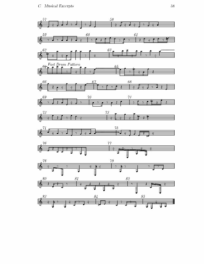
C. Musical Excerpts 58G57 ! @ ! ! ! ? ! ! ? ! ! 58 @ ! @ ! @ .! ? ! @ !G59 ? ! ? ! ! .> ! @ 60 ? ! > ! ! ! ? ! ? 61 ..> ! @ .! ! .? 4!zG62{4! @ ! @ .! ! .! ! ? ! @ 63 ! @ ! ! @ ! ! .? ! @ !zG64 Fast Drum Pattern{! ! ! ! ? ! @ ! ! .? !z 65{! ! ? 4! @ ! ! .>G66 ! > ! @ ! @ ! > !z 67{! ? ! .? ! .> 68 @ ! @ ! .? ! ..> !G69 .? ! ..> ! ! @ ! ? 70 .! ? ! .? ! > ! 71 ? ! ? .! 4! @ ! ..>G72 @ ! ..> ! .? ! ! @ 73 @ ! @ .! @ ! 4! > 6!G74 ! @ ! .? ! ! ? ! @ ! !z 75{ .! @ ! ! ! > 4! @G76 ! > ! ! @ ! .? ! ! 77 @ ! .> ! ? ! @EEEE! @G78 @ ! ?OO! ? ! @ )! @ 79 ? )! ? ! .? ! ? !G80 .> ! ..> ! ? 81 @ ! > ! > ! @ ! @ 82 ? ! ..> ! ?OOOO! @G83 @ )! .? ! @ ! ? ! @ 84 4! ! @ ! .? ! ? ! 85 ! ! @ ! !

C. Musical Excerpts 59\Controlled" Simulation of Jules 1by Yuval Marom and S-PlusG 44 Slow Drum Pattern! ! ? ! ! ! > 2 ! ! .? .! ? ! @G 3 @ ! ? ! ! ! .> ! @ 4 @ ! @ ! @ ! @ 4! ! ..>G 5 .> 4! > 4! @ 6! @ 6 ! ! .? .2! ! ! .! @ !z 7{! ? ! ? ! > ! @ !zG 8{! > ! ! @ ! ! .? !z 9{! ! ! ? ! ? ! ! .! @ !G10 ? ! > ! ..> ! ! 11 .> ! ? !��! ?��!z 12{! ? .! ? ! .! >G13 ! > ! @ ! .? ! ! ? 14 @ ! ! .? ! ! > ! @G15 ..> ! ? ! ! > 4!z 16{4! ..> 6! ? ! ! @ ! ? 17 ! .? ! ! .? .! ! .!G18 ! ! .? ! ? ! )! .? 19 ? ! @ ! .! �����! ? .! 20 .4! .? ! ..> 6! .?G21 Fast Drum Pattern.! ! ? ! ! > ! ? 22 @ ! ? ! ! .> !z 23{! ? ! .? ! ?��! ?��! @G24 .? ! @ ! @ ! @ ! .? 25 ! .? ! ! .. ? ! @ !zG26{! @ ! ! .> ! @ ! ? 27 ? ! ..> ! ..> !z 28{! ! .? ! ! ..> !G29 ! @ ! ? ! .! ! ! @ ! @ 30 ? ! ! ? ! ? ! @ ! !G31 ! .. .2! !z 32{! ..! ? !z 33{! ..> ! ! ? ! ?

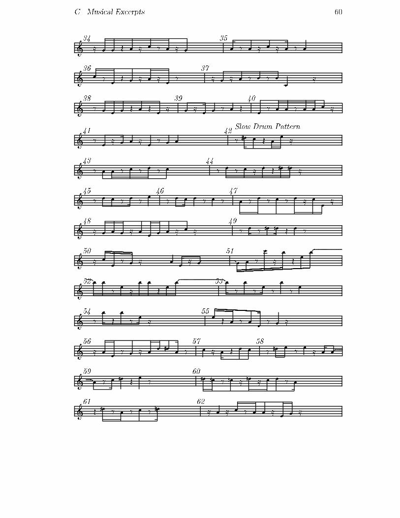
C. Musical Excerpts 60G34 @ ! ! > ! @ ! ? ! @ ! 35 ! ? ! @ ! @ ! .? .!G36 ! ? ! > ! @ ! @ ! ? 37 @ ! @ ! ? ! ? ! ! @G38 ? ! ! ! > ! > ! @ 39 .! @ ! ! ? ! .> 40 .! .? ! ! .? ! ! ! @G41 .? ! @ ! ! @ ! ? ! ! 42 Slow Drum Pattern.? 4! .! .> ! ! @G43 ? ! ! ? ! ? ! .? ! 44 ? ! ? ! @ ! ..> 4! 6! @G45 ? ! .! .? ! .? ! 46 ? .! ! .! ? .! ? 47 ! ? ! ? ! .? ! @ ! ! @G48 @ ! ! ! @ ! ! ! ! @ .! @ 49 ? ! ? 4! 6! > ! ?G50 @ ! ! .?DDDD! @ ! ! @ !z 51{! ! .? ! @��! > !��!zG52{! ! ? ! @ ! ! .> ! !z 53{! ? .! ? ! ? ! ? !G54 .? ! .> ! ? ! @ 55 ! >CC! ? ! AAEE! ? ! @G56 @ ! ! ? ! @ ! ! 4! ! .? 57 ! @ ! ..> ! .! 58 ? 4! ! .? ! ..@ ! !zG59{! ? ! 4! .> ! ? 60 4! 4! ? 6! @ 6! @ ! ! .? !G61 > 4! ? ! ? ! .? 6! 62 @ ! @ ! ? ! ! @ ! ! @

C. Musical Excerpts 61G63 ! ! .? ! > ! ! ? 64 Fast Drum Pattern.? ! .. ! .> !z 65{! ! >DD! @ ! AAEE! .? !zG66{! ? ! @ ! ? ! ! @ ! ! !z 67{! @ ! ! .> ! ? !G68 ! @ ! @ ! ? ! @ ! @ ! .? 69 @ ! .? ! > ! ! .? !zG70{ )! ? ! ..? ! @ ! @ !z 71{! @ ! ! ! @ ! 72 @@@! ? ! ..> !BBEE! >G73 ! ! ? ! .? .! ! ! @ 74 ? ! ! > ! ? ! @ !zG75{ AA! .! .> ! ?EE! 76 ! ? !BB! .> !EE! 77 ? .! ! > ! @ ����! @G78 ? ! @ ! ! 2! @ ! @ !�����! ? 79 ! @ ! @ ! .> !KKKK! ?G80 ! ? .! ! .? ! 4! ? 81 .> ! ! .? ! ! @ !z 82{! ? ! ..> ! .? !G83 ! .? ! 4! > ! .! ! 84 @ ! @ ! .! ! @ ! ! ! ? !G85 ..> ! 4! ? .! @ ! 86 ! ? ! @ ! @ !

APPENDIX DOriginal Honours ProposalTitle: Stochastic Techniques for Computer-Music CompositionAuthor: Yuval MaromSupervisors: Assoc. Prof. C.P. Tsang (Computer Science)Prof. Adrian Baddeley (Mathematics)D.1 BackgroundMusic is a form of human artistic creation. The concept of creation an on go-ing issue in Arti�cial Intelligence and speci�cally in Computer Music. In partic-ular: can the computer imitate it? Xenakis (1971) suggested that the creativethought of man gives birth to \mental machines", which are merely sets of con-straints and choices. Some of these mechanisms can be expressed in mathemati-cal terms [1, Chapter 1].Xenakis claims that musical composition o�ers a collection of sequences that itwishes to be causal, but strict, deterministic causality needs to be replaced by amore general causality, by a probabilistic logic. It was through musical necessitythat the laws of calculus of probabilities entered composition.Choices play a signi�cant role in the process of musical composition and this iswhere statistics come into the picture. Granted a basic hypothesis, probabilitytheory provides us with choosing tools. Statistics provide quantitative tools fortreating an issue previously dealt with solely by qualitative means: the issue ofbalance in a sequence of music [2]. Balance refers to the relative stresses accordedto di�erent musical resources and its formal representation is the statistical dis-tribution [3].Stochastic processes are processes that develop in time in a manner controlled byprobabilistic laws. They deal with the behavior of a collection of random vari-ables and their interdependence [4].The use of statistics in the �eld of music composition remains worth of atten-tion. More common techniques that have of been employed in this area are ma-62

D. Original Honours Proposal 63chine learning ones, such as Neural Nets and rule-based systems.D.2 AimThe aim of this project is to test whether stochastic processes can imitate themental processes of a human composer, without considering the psychology as-sociated with such processes. This project can therefore be seen as an experi-ment, where di�erent stochastic models will be considered and the level of suc-cess of each one in generating "good" music will be examined.Results from this project could be extended to other arts and other activitiesperformed by humans that require creative thought and which we wish to auto-mate. The outcome of this project could have signi�cant implications to Arti�-cial Intelligence and Cognitive Science.D.3 MethodsThe application used in this project will be Jazz. The reasons for this are:� It is relatively simple. Even the simplest Jazz pieces are very good.� In composing such music the composer includes:1. Some randomness (with regards to pitch, intensity etc')2. Some choices (for the same dimensions as in 1 above)3. Repetitions4. PatternsAnd hopefully we can model all of the above together using stochastic tech-niques.The project will consist of three parts, where the third part will depend on thesuccess of the second one:Initial study of the musicTo be able to choose which models are appropriate and how their parametersshould be set, some musical research needs to be done. The musical style and itscharacteristics should be well known. This will be achieved by reading about jazz,listening to some standard pieces of jazz and maybe even talking to musicians.

D. Original Honours Proposal 64Modeling & simulating - Analysis by synthesisThe main emphasis of this project will be to choose stochastic models which bestdescribe the di�erent characteristics of jazz. Simulations of these models willthen be performed to generate (compose) sequences of jazz.The most common stochastic models are Markov Chains (MC's) and consequentlymost of the project time will be devoted to analyzing their di�erent variations.Some examples are: simple MC's, k-dependent MC's, \state incorporation", hid-den Markov models, and random walks.This part will involve two stages:1. Initially, simple models will be considered to get a feel for the appropriate-ness of the stochastic techniques in the compositional process. The tasksof observing the behavior of these models and adjusting their parametersas required will be easier when simple models are used.2. Once the details about the parameters of the models are determined toour satisfaction (ie results lie within the bounds of acceptable music), morecomplicated models, which might be more realistic, will be considered. Thisstage will also involve some �ne-tuning of the parameters according to theperformances of the simulations.The statistical software used will be Splus and either a PC or a Sun running X-Windows will be used to run it.The output data from the simulations will need to be converted to midi format -a small program will be created which performs this. A midi-interface package,such as Common Music and Cakewalk, will be used to play the resulting midi �lethrough a Roland U220 sound module.There needs to be a methodology to test the results of this experiment. The sim-plest, and probably best, way of doing this is to use a human's opinion | afterall, music is for the enjoyment of humans. Objectiveness is very important here,so the author will try to be as objective as possible and will also use a panel ofcritiques, who will give their opinions as to \how good" the results sound.Fitting the models to real dataThe previous part of the project will be considered a success if adequate modelsare developed. That is, if the simulations based on these models produce goodresults. Depending on this success, and if time permits, an attempt will be madeto �t the models to real data coming from real jazz pieces.The collection of such data will be achieved either by:� Inviting a jazz musician to play some music, or

D. Original Honours Proposal 65� Using some benchmark jazz recordings.The purpose here is to further strengthen the adequacy of the result and see howwell they can model real situations.References1. Iannis Xenakis. Formalised Music. Indiana University Press, Bloomington,Ind, 1971.2. Charles Ames. A catalog of statistical distributions: Techniques for trans-forming random, deterministic and chaotic sequences. Leonardo Music Jour-nal, 1(1):55{70, 1991.3. Charles Ames. Statistical and compositional balance. Perspectives of NewMusic, 28(1):80, 1990.4. Emanuel Parzen. Stochastic Processes. Holden-Day, Inc., San Francisco, 1962.