Improving Sequential Feature Selection Methods' Performance by Means of Hybridization

IMPROVING SEQUENTIAL FEATURE SELECTION METHODS’PERFORMANCE BY MEANS OF HYBRIDIZATION

Petr Somol and Jana NovovicovaDepartment of Pattern Recognition

Institute of Information Theory and AutomationAcademy of Sciences of the Czech Republic

CZ18208 Prague 8email: {somol, novovic}@utia.cas.cz

Pavel PudilFaculty of Management

Prague University of EconomicsJarosovska 1117/II

CZ37701, Jindrichuv Hradecemail: [email protected]

ABSTRACTIn this paper we propose the general scheme of defining hy-brid feature selection algorithms based on standard sequen-tial search with the aim to improve feature selection per-formance, especially on high-dimensional or large-sampledata. We show experimentally that “hybridization” has notonly the potential to dramatically reduce FS search time,but in some cases also to actually improve classifier gener-alization, i.e., its classification performance on previouslyunknown data.

KEY WORDS

sification performance, subset search, statistical patternrecognition

1 Introduction

A broad class of decision-making problems can be solvedby learning approach. This can be a feasible alternativewhen neither an analytical solution exists nor the mathe-matical model can be constructed. In these cases the re-quired knowledge can be gained from the past data whichform the so-called learning or training set. Then the for-mal apparatus of statistical pattern recognition can be usedto learn the decision-making. The first and essential stepof statistical pattern recognition is to solve the problem offeature selection (FS) or more generally dimensionality re-duction (DR). The problem of effective feature selection– especially in case of high-dimensional and large-sampleproblems – will be of primary focus in this paper.

1.1 Feature Subset Selection

Given a set Y of |Y| features, let us denote Xd the set ofall possible subsets of size d, where d represents the de-sired number of features. Let J(X) be a criterion functionthat evaluates feature subset X ∈ Xd. Without any loss ofgenerality, let us consider a higher value of J to indicatea better feature subset. Then the feature selection problemcan be formulated as follows: Find the subset Xd for which

J(Xd) = maxX∈Xd

J(X). (1)

Assuming that a suitable criterion function has been chosento evaluate the effectiveness of feature subsets, feature se-lection is reduced to a search problem that detects an opti-mal feature subset based on the selected measure. Note thatthe choice of d may be a complex issue depending on prob-lem characteristics, unless the d value can be optimized aspart of the search process.

An overview of various aspects of feature selectioncan be found in [1], [2], [3], [4]. Many existing featureselection algorithms designed with different evaluation cri-teria can be categorized as filter [5], [6] wrapper [7], hy-brid [8], [9], [10] or embedded [11], [12], [13] or [14],[15]. Filter methods are based on performance evaluationfunctions calculated directly from the training data such asdistance, information, dependency, and consistency, [16, 1]and select features subsets without involving any learningalgorithm. Wrapper methods require one predeterminedlearning algorithm and use its estimated performance asthe evaluation criterion. They attempt to find features bet-ter suited to the learning algorithm aiming to improve per-formance. Generally, the wrapper method achieves betterperformance than the filter method, but tends to be morecomputationally expensive than the filter approach. Also,the wrappers yield feature subsets optimized for the givenlearning algorithm only - the same subset may thus be badin another context.

In the following we will investigate the hybrid ap-proach to FS that combines the advantages of filter andwrapper algorithms to achieve best possible performancewith a particular learning algorithm with the time complex-ity comparable to that of the filter algorithms. In Section 2an overview of sequential search FS methods is given. Wedistinguish methods that require the subset size to be speci-fied by user (Sect. 2.1 to 2.6) from methods capable of sub-set size optimization (Sect. 2.7). The general scheme of hy-bridization is introduced in Sect. 3. Section 4 describes theperformed experiments and Sect. 5 summarizes and con-cludes the paper.

2 Sub-Optimal Search Methods

Provided a suitable FS criterion function (cf. [16]) is avail-able, the only tool needed is the search algorithm that gen-

Feature selection, sequential search, hybrid methods, clas-

689-001 1

erates a sequence of subsets to be tested. Despite theadvances in optimal search ([17], [18]), for larger thanmoderate-sized problems we have to resort to sub-optimalmethods. Very large number of various methods exists.The FS framework includes approaches that take use ofevolutionary (genetic) algorithms ([19]), tabu search ([20]),or ant colony ([21]). In the following we present a basicoverview over several tools that are useful for problems ofvarying complexity, based mostly on the idea of sequentialsearch (Section 2.2 [16]). Finally, we show a general wayof defining hybrid versions of sequential FS algorithms.

An integral part of any FS process is the decisionabout the number of features to be selected. Determin-ing the correct subspace dimensionality is a difficult prob-lem beyond the scope of this chapter. Nevertheless, in thefollowing we will distinguish two types of FS methods:d-parametrized and d-optimizing. Most of the availablemethods are d-parametrized, i.e., they require the user todecide what cardinality should the resulting feature subsethave. In Section 2.7 a d-optimizing procedure will be de-scribed, that optimizes both the feature subset size and itscontents at once, provided the suitable criterion is available(classifier accuracy in wrappers can be used while mono-tonic probabilistic measures can not).

2.1 Best Individual Feature

The Best Individual Feature (BIF) approach is the simplestapproach to FS. Each feature is first evaluated individu-ally using the chosen criterion. Subsets are then selectedsimply by choosing the best individual features. This ap-proach is the fastest but weakest option. It is often theonly applicable approach to FS in problems of very high di-mensionality. BIF is standard in text categorization ([22],[23]), genetics ([24], [25]) etc. BIF may be preferable inother types of problems to overcome FS stability problems.However, more advanced methods that take into account re-lations among features are likely to produce better results.Several of such methods are discussed in the following.

2.2 Sequential Search Framework

To simplify further discussion let us focus only on the fam-ily of sequential search methods. Most of the known se-quential FS algorithms share the same “core mechanism”of adding and removing features to/from a current sub-set. The respective algorithm steps can be described asfollows (for the sake of simplicity we consider only non-generalized algorithms that process one feature at a timeonly):

Definition 1 For a given current feature set Xd, let f+ bethe feature such that

f+ = arg maxf∈Y\Xd

J+(Xd, f) , (2)

where J+(Xd, f) denotes the criterion function used toevaluate the subset obtained by adding f (f ∈ Y \ Xd)

to Xd. Then we shall say that ADD(Xd) is an operation ofadding feature f+ to the current set Xd to obtain set Xd+1

if

ADD(Xd) ≡ Xd∪{f+} = Xd+1, Xd, Xd+1 ⊂ Y. (3)

Definition 2 For a given current feature set Xd, let f− bethe feature such that

f− = arg maxf∈Xd

J−(Xd, f) , (4)

where J−(Xd, f) denotes the criterion function used toevaluate the subset obtained by removing f (f ∈ Xd) fromXd. Then we shall say that RMV (Xd) is an operation ofremoving feature f− from the current set Xd to obtain setXd−1 if

RMV (Xd) ≡ Xd\{f−} = Xd−1, Xd, Xd−1 ⊂ Y. (5)

In order to simplify the notation for a repeated appli-cation of FS operations we introduce the following usefulnotation

Xd+2 = ADD(ADD(Xd)) = ADD2(Xd) , (6)

Xd−2 = RMV (RMV (Xd)) = RMV 2(Xd) ,

and more generally

Xd+δ = ADDδ(Xd), Xd−δ = RMV δ(Xd) . (7)

Note that in standard sequential FS methods J+(·) andJ−(·) stand for

J+(Xd, f) = J(Xd ∪ {f}), (8)

J−(Xd, f) = J(Xd \ {f}) ,

where J(·) is either a filter- or wrapper-based criterionfunction ([26]) to be evaluated on the subspace defined bythe tested feature subset.

2.3 Simplest Sequential Selection

The basic feature selection approach is to build up a sub-set of required number of features incrementally startingwith the empty set (bottom-up approach) or to start withthe complete set of features and remove redundant featuresuntil d features retain (top-down approach). The simplest(among recommendable choices) yet widely used sequen-tial forward (or backward) selection methods, SFS andSBS ([27], [16]), iteratively add (remove) one feature ata time so as to maximize the intermediate criterion valueuntil the required dimensionality is achieved.

SFS (Sequential Forward Selection) yielding a subset of dfeatures:

1. Xd = ADDd(∅).

2

As many other of the earlier sequential methods both SFSand SBS suffer from the so-called nesting of feature subsetswhich significantly deteriorates optimization ability. Thefirst attempt to overcome this problem was to employ ei-ther the Plus-l-Take away-r (also known as (l, r)) or gen-eralized (l, r) algorithms ([16]) which involve successiveaugmentation and depletion process. The same idea in aprincipally extended and refined form constitutes the basisof Floating Search.

2.4 Sequential Floating Search

The Sequential Forward Floating Selection (SFFS) ([28])procedure consists of applying after each forward step anumber of backward steps as long as the resulting subsetsare better than previously evaluated ones at that level. Con-sequently, there are no backward steps at all if intermedi-ate result at actual level (of corresponding dimensionality)cannot be improved. The same applies for the backwardversion of the procedure. Both algorithms allow a ’self-controlled backtracking’ so they can eventually find goodsolutions by adjusting the trade-off between forward andbackward steps dynamically. In a certain way, they com-pute only what they need without any parameter setting.

SFFS (Sequential Forward Floating Selection) yielding asubset of d features, with optional search-restricting param-eter ∆ ∈ [0, D − d]:

1. Start with X0 = ∅, k = 0.

2. Xk+1 = ADD(Xk), k = k + 1.

3. Repeat Xk−1 = RMV (Xk), k = k − 1 as long as itimproves solutions already known for the lower k.

4. If k < d + ∆ go to step 2.

A detailed formal description of this now classical pro-cedure can be found in [28]. The backward counterpartto SFFS is the Sequential Backward Floating Selection(SBFS). Its principle is analogous.

Floating search algorithms can be considered univer-sal tools not only outperforming all predecessors, but alsokeeping advantages not met by more sophisticated algo-rithms. They find good solutions in all problem dimen-sions in one run. The overall search speed is high enoughfor most of practical problems. The idea of Floating searchhas been futher developed in [29] and [30].

2.5 Oscillating Search

The more recent Oscillating Search (OS) ([31]) can be con-sidered a “meta” procedure, that takes use of other featureselection methods as sub-procedures in its own search. Theconcept is highly flexible and enables modifications for dif-ferent purposes. It has shown to be very powerful and ca-pable of over-performing standard sequential procedures,

including Floating Search algorithms. Unlike other meth-ods, the OS is based on repeated modification of the currentsubset Xd of d features. In this sense the OS is independentof the predominant search direction. This is achieved byalternating so-called down- and up-swings. Both swingsattempt to improve the current set Xd by replacing someof the features by better ones. The down-swing first re-moves, then adds back, while the up-swing first adds, thenremoves. Two successive opposite swings form an oscilla-tion cycle. The OS can thus be looked upon as a controlledsequence of oscillation cycles. The value of o denoted os-cillation cycle depth determines the number of features tobe replaced in one swing. o is increased after unsuccessfuloscillation cycles and reset to 1 after each Xd improvement.The algorithm terminates when o exceeds a user-specifiedlimit ∆. The course of Oscillating Search is illustrated incomparison to SFS and SFFS in Fig. 1. Every OS algorithm

Figure 1. Graphs demonstrate the course of d-parametrized search algorithms: a) Sequential ForwardSelection, b) Sequential Forward Floating Selection, c) Os-

requires some initial set of d features. The initial set maybe obtained randomly or in any other way, e.g., using someof the traditional sequential selection procedures. Further-more, almost any feature selection procedure can be usedin up- and down-swings to accomplish the replacements offeature o-tuples.

OS (Oscillating Search) yielding a subset of d features,with optional search-restricting parameter ∆ ≥ 1:

1. Start with initial set Xd of d features. Set cycle depthto o = 1.

2. Let X↓d = ADDo(RMV o(Xd)).

3. If X↓d better than Xd, let Xd = X↓d, let o = 1 and goto step 2.

4. Let X↑d = RMV o(ADDo(Xd)).

cillating Search.

3

5. If X↑d better than Xd, let Xd = X↑d, let o = 1 and goto step 2.

6. If o < ∆ let o = o + 1 and go to step 2.

The generality of OS search concept allows to adjust thesearch for better speed or better accuracy (by adjusting ∆,redefining the initialization procedure or redefining ADD /RMV). As opposed to all sequential search procedures, OSdoes not waste time evaluating subsets of cardinalities toodifferent from the target one. This ”focus” improves theOS ability to find good solutions for subsets of given car-dinality. The fastest improvement of the target subset maybe expected in initial phases of the algorithm, because ofthe low initial cycle depth. Later, when the current featuresubset evolves closer to optimum, low-depth cycles fail toimprove and therefore the algorithm broadens the search(o = o + 1). Though this improves the chance to get closerto the optimum, the trade-off between finding a better solu-tion and computational time becomes more apparent. Con-sequently, OS tends to improve the solution most consider-ably during the fastest initial search stages. This behavioris advantageous, because it gives the option of stopping thesearch after a while without serious result-degrading con-sequences. Let us summarize the key OS advantages:

• It may be looked upon as a universal tuning mech-anism, being able to improve solutions obtained inother way.

• The randomly initialized OS is very fast, in case ofvery high-dimensional problems may become the onlyapplicable alternative to BIF. For example, in docu-ment analysis ([32]) for search of the best 1000 wordsout of a vocabulary of 10000 all other sequential meth-ods prove to be too slow.

• Because the OS processes subsets of target cardinalityfrom the very beginning, it may find solutions evenin cases, where the sequential procedures fail due tonumerical problems.

• Because the solution improves gradually after each os-cillation cycle, with the most notable improvements atthe beginning, it is possible to terminate the algorithmprematurely after a specified amount of time to obtaina usable solution. The OS is thus suitable for use inreal-time systems.

• In some cases the sequential search methods tend touniformly get caught in certain local extremes. Run-ning the OS from several different random initialpoints gives better chances to avoid that local extreme.

2.6 Experimental Comparison of d-ParametrizedMethods

The d-parametrized sub-optimal FS methods as discussedin preceding sections 2.1 to 2.5 have been listed in the order

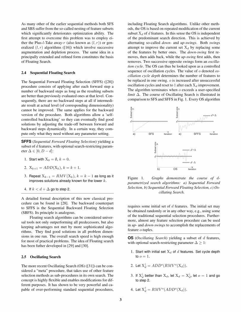
of their speed-vs-optimization performance characteristics.The BIF is the fastest but worst performing method, OS of-fers the strongest optimization ability at the cost of slowestcomputation (although it can be adjusted differently). Toillustrate this behavior we compare the output of BIF, SFS,SFFS and OS on a FS task in wrapper ([7]) setting.

The methods have been used to find best feature sub-sets for each subset size d = 1, . . . , 34 on the ionospheredata (34 dim., 2 classes: 225 and 126 samples) from theUCI Repository ([33]). The dataset had been split to 80%train and 20% test part. FS has been performed on the train-ing part using 10-fold cross-validation, in which 3-NearestNeighbor classifier was used as FS criterion. BIF, SFS andSFFS require no parameters, OS had been set to repeat eachsearch 15× from different random initial subsets of givensize, with ∆ = 15. This set-up is highly time consumingbut enables avoiding many local extremes that would notbe avoided by other algorithms.

Figure 2 shows the maximal criterion value obtainedby each method for each subset size. It can be seen thatthe strongest optimizer in most of cases is OS, althoughSFFS falls behind just negligibly. SFS optimization abilityis shown to be markedly lower, but still higher than that ofBIF.

Figure 2. Sub-optimal FS methods’ optimization perfor-

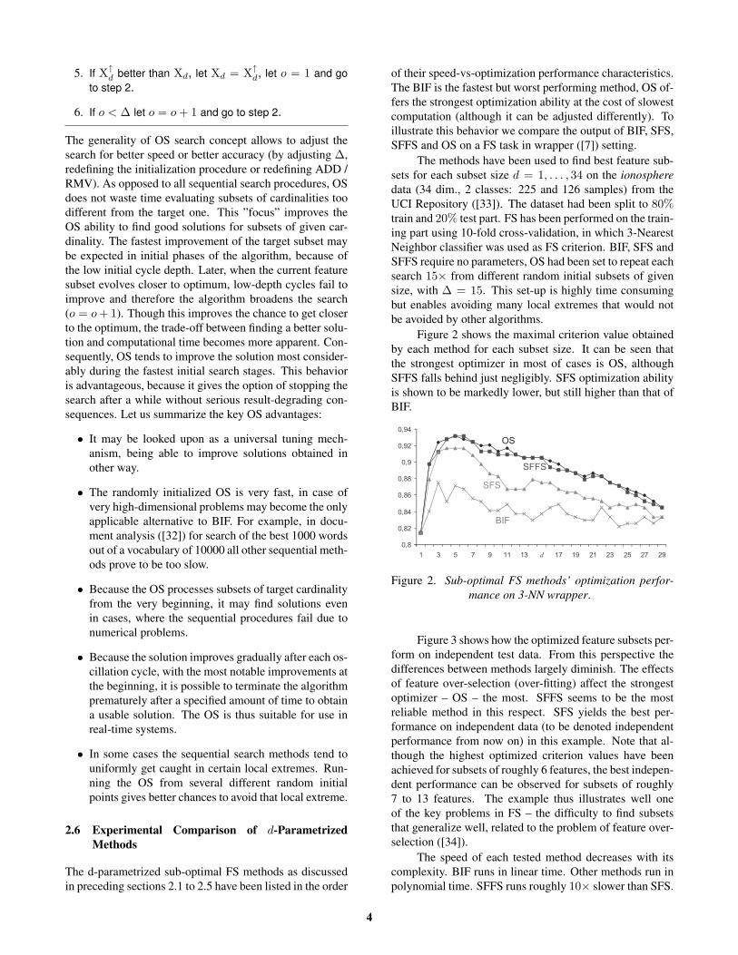
Figure 3 shows how the optimized feature subsets per-form on independent test data. From this perspective thedifferences between methods largely diminish. The effectsof feature over-selection (over-fitting) affect the strongestoptimizer – OS – the most. SFFS seems to be the mostreliable method in this respect. SFS yields the best per-formance on independent data (to be denoted independentperformance from now on) in this example. Note that al-though the highest optimized criterion values have beenachieved for subsets of roughly 6 features, the best indepen-dent performance can be observed for subsets of roughly7 to 13 features. The example thus illustrates well oneof the key problems in FS – the difficulty to find subsetsthat generalize well, related to the problem of feature over-selection ([34]).

The speed of each tested method decreases with itscomplexity. BIF runs in linear time. Other methods run inpolynomial time. SFFS runs roughly 10× slower than SFS.

mance on 3-NN wrapper.

4

OS in the slow test setting runs roughly 10 to 100× slowerthan SFFS. The speed penalty of more complex methodsgets even more notable with increasing dimensionality andsample size.

Figure 3. Sub-optimal FS methods’ performance verified

2.7 Dynamic Oscillating Search – The d-optimizingMethod

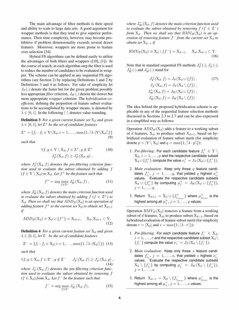
The idea of Oscillating Search (Sect. 2.5) has been furtherextended in form of the Dynamic Oscillating Search (DOS)([35]). The DOS algorithm can start from any initial sub-set of features (including empty set). Similarly to OS itrepeatedly attempts to improve the current set by means ofrepeating oscillation cycles. However, the current subsetsize is allowed to change, whenever a new globally best so-lution is found at any stage of the oscillation cycle. Unlikeother methods discussed in this chapter the DOS is thus ad-optimizing procedure.

k+D

k-D

k

0 DOS Iteration

Su

bse

t siz

e

Figure 4. The DOS course of search

The course of Dynamic Oscillating Search is illus-trated in Fig. 4. See Fig. 1 for comparison with OS, SFFSand SFS. Similarly to OS the DOS terminates when thecurrent cycle depth exceeds a user-specified limit ∆. TheDOS also shares with OS the same advantages as listed inSect. 2.5: the ability to tune results obtained in a differentway, gradual result improvement, fastest improvement ininitial search stages, etc.

DOS (Dynamic Oscillating Search) yielding a subset ofoptimized size k, with optional search-restricting param-eter ∆ ≥ 1:

1. Start with Xk = ADD(ADD(∅)), k = 2. Set cycledepth to δ = 1.

2. Compute ADDδ(RMV δ(Xt)); if any intermediatesubset Xi, i ∈ [k − δ, k] is found better than Xk,let it become the new Xk with k = i, let δ = 1 andrestart step 2.

3. Compute RMV δ(ADDδ(Xt)); if any intermediatesubset Xj , j ∈ [k, k + δ] is found better than Xk,let it become the new Xk with k = j, let δ = 1 and goto step 2.

4. If δ < ∆ let δ = δ + 1 and go to step 2.

In the course of search the DOS generates a sequence ofsolutions with ascending criterion values and, provided thecriterion value does not decrease, decreasing subset size.The search time vs. closeness-to-optimum trade-off canthus be handled by means of pre-mature search interrup-tion. The number of criterion evaluations is in the O(n3)order of magnitude. Nevertheless, the total search time de-pends heavily on the chosen ∆ value, on particular dataand criterion settings, and on the unpredictable number ofoscillation cycle restarts that take place after each solutionimprovement. Note: with monotonic criteria DOS yieldsalways the full feature set. This behavior makes it un-usable with many probabilistic distance measures (Bhat-tacharyya distance etc.). Nevertheless, DOS performs wellwith wrapper FS criteria (classifier accuracy).

3 Hybrid Algorithms – Improving FeatureSelection Performance

Filter methods [26] for feature selection are general pre-processing algorithms that do not rely on any knowledge ofthe learning algorithm to be used. They are distinguishedby specific evaluation criteria including distance, informa-tion, dependency. Since the filter methods apply indepen-dent evaluation criteria without involving any learning al-gorithm they are computationally efficient. Wrapper meth-ods [26] require a predetermined learning algorithm insteadof an independent criterion for subset evaluation. Theysearch through the space of feature subsets using a learningalgorithm, calculate the estimated accuracy of the learn-ing algorithm for each feature before it can be added toor removed from the feature subset. It means, that learn-ing algorithms are used to control the selection of featuresubsets which are consequently better suited to the prede-termined learning algorithm. Due to the necessity to trainand evaluate the learning algorithm within the feature se-lection process, the wrapper methods are more computa-tionally expensive than the filter methods.

using 3-NN on independent data.

.

5

The main advantage of filter methods is their speedand ability to scale to large data sets. A good argument forwrapper methods is that they tend to give superior perfor-mance. Their time complexity, however, may become pro-hibitive if problem dimensionality exceeds several dozenfeatures. Moreover, wrappers are more prone to featureover-selection [34].

Hybrid FS algorithms can be defined easily to utilizethe advantages of both filters and wrappers ([10], [1]). Inthe course of search, in each algorithm step the filter is usedto reduce the number of candidates to be evaluated in wrap-per. The scheme can be applied in any sequential FS algo-rithms (see Section 2) by replacing Definitions 1 and 2 byDefinitions 3 and 4 as follows. For sake of simplicity letJF (.) denote the faster but for the given problem possiblyless appropriate filter criterion, JW (.) denote the slower butmore appropriate wrapper criterion. The hybridization co-efficient, defining the proportion of feature subset evalua-tions to be accomplished by wrapper means, is denoted byλ ∈ [0, 1]. In the following d·e denotes value rounding.

Definition 3 For a given current feature set Xd and givenλ ∈ [0, 1], let Z+ be the set of candidate features

Z+ = {fi : fi ∈ Y\Xd; i = 1, . . . , max{1, dλ·|Y\Xd|e}}(9)

such that

∀f, g ∈ Y \Xd, f ∈ Z+, g /∈ Z+ (10)

J+F (Xd, f) ≥ J+

F (Xd, g) ,

where J+F (Xd, f) denotes the pre-filtering criterion func-

tion used to evaluate the subset obtained by adding f(f ∈ Y \Xd) to Xd. Let f+ be the feature such that

f+ = arg maxf∈Z+

J+W (Xd, f) , (11)

where J+W (Xd, f) denotes the main criterion function used

to evaluate the subset obtained by adding f (f ∈ Z+) toXd. Then we shall say that ADDH(Xd) is an operation ofadding feature f+ to the current set Xd to obtain set Xd+1

if

ADDH(Xd) ≡ Xd ∪ {f+} = Xd+1, Xd, Xd+1 ⊂ Y.(12)

Definition 4 For a given current feature set Xd and givenλ ∈ [0, 1], let Z− be the set of candidate features

Z− = {fi : fi ∈ Xd; i = 1, . . . , max{1, dλ·|Xd|e}} (13)

such that

∀f, g ∈ Xd, f ∈ Z−, g /∈ Z− J−F (Xd, f) ≥ J−F (Xd, g) ,(14)

where J−F (Xd, f) denotes the pre-filtering criterion func-tion used to evaluate the subset obtained by removing f(f ∈ Xd) from Xd. Let f− be the feature such that

f− = arg maxf∈Z−

J−W (Xd, f), (15)

where J−W (Xd, f) denotes the main criterion function usedto evaluate the subset obtained by removing f (f ∈ Z−)from Xd. Then we shall say that RMVH(Xd) is an op-eration of removing feature f− from the current set Xd toobtain set Xd−1 if

RMVH(Xd) ≡ Xd \ {f−} = Xd−1, Xd, Xd−1 ⊂ Y.(16)

Note that in standard sequential FS methods J+F (·), J−F (·),

J+W (·) and J−W (·) stand for

J+F (Xd, f) = JF (Xd ∪ {f}) , (17)

J−F (Xd, f) = JF (Xd \ {f}) ,

J+W (Xd, f) = JW (Xd ∪ {f}) ,

J−W (Xd, f) = JW (Xd \ {f}) .

The idea behind the proposed hybridization scheme is ap-plicable in any of the sequential feature selection methodsdiscussed in Sections 2.3 to 2.7 and can be also expressedin a simplified way as follows:

Operation ADDH(Xd) adds a feature to a working subsetof d features, Xd, to produce subset Xd+1, based on hy-bridized evaluation of feature subset merit (for simplicitydenote p = |Y \Xd| and q = max{1, dλ · pe}):

1. Pre-filtering: For each candidate feature f+i ∈ Y \

Xd, i = 1, . . . , p and the respective candidate subsetXd∪{f+

i } compute the value ν+i = JF (Xd∪{f+

i }).

2. Main evaluation: Keep only those q feature candi-dates f+

ij, j = 1, . . . , q, that yielded q highest ν+

ij

values. Evaluate the respective candidate subsetsXd ∪ {f+

ij} by computing µ+

j = JW (Xd ∪ {f+ij}),

j = 1, . . . , q.

3. Return Xd+1 = Xd ∪ {f+ijmax

} where µ+jmax

is the

highest among all µ+j , j = 1, . . . , q values.

Operation RMVH(Xd) removes a feature from a workingsubset of d features, Xd, to produce subset Xd−1, based onhybridized evaluation of feature subset merit (for simplicitydenote r = |Xd| and s = max{1, dλ · re}):

1. Pre-filtering: For each candidate feature f−i ∈ Xd,i = 1, . . . , r and the respective candidate subset Xd \{f−i } compute the value ν−i = JF (Xd \ {f−i }).

2. Main evaluation: Keep only those s feature candi-dates f−ij

, j = 1, . . . , s, that yielded s highest ν−ij

values. Evaluate the respective candidate subsetsXd \ {f−ij

} by computing µ−j = JW (Xd \ {f−ij}),

j = 1, . . . , s.

3. Return Xd−1 = Xd \ {f−ijmax} where µ−jmax

is the

highest among all µ−j , j = 1, . . . , s values.

6

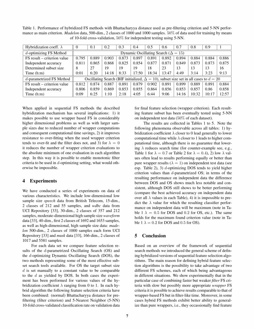
Table 1. Performance of hybridized FS methods with Bhattacharyya distance used as pre-filtering criterion and 5-NN perfor-mance as main criterion. Madelon data, 500-dim., 2 classes of 1000 and 1000 samples. 50% of data used for training by means

of 10-fold cross-validation, 50% for independent testing using 5-NN.

Hybridization coeff. λ 0 0.1 0.2 0.3 0.4 0.5 0.6 0.7 0.8 0.9 1d-optimizing FS Method Dynamic Oscillating Search (∆ = 15)FS result – criterion value 0.795 0.889 0.903 0.873 0.897 0.891 0.892 0.894 0.884 0.884 0.886Independent accuracy 0.811 0.865 0.868 0.825 0.854 0.877 0.871 0.849 0.873 0.873 0.875Determined subset size 8 27 19 19 19 18 23 13 13 13 16Time (h:m) 0:01 6:20 14:18 8:33 17:50 18:34 13:47 4:49 3:14 3:23 9:13d-parametrized FS Method Oscillating Search (BIF initialized, ∆ = 10), subset size set in all cases to d = 20FS result – criterion value 0.812 0.874 0.887 0.891 0.879 0.902 0.891 0.899 0.889 0.891 0.884Independent accuracy 0.806 0.859 0.869 0.853 0.855 0.864 0.856 0.853 0.857 0.86 0.858Time (h:m) 0:09 6:25 1:10 2:18 4:05 6:44 9:06 14:16 10:32 10:17 12:57

When applied in sequential FS methods the describedhybridization mechanism has several implications: 1) itmakes possible to use wrapper based FS in considerablyhigher dimensional problems as well as with larger sam-ple sizes due to reduced number of wrapper computationsand consequent computational time savings, 2) it improvesresistance to over-fitting when the used wrapper criteriontends to over-fit and the filter does not, and 3) for λ = 0it reduces the number of wrapper criterion evaluations tothe absolute minimum of one evaluation in each algorithmstep. In this way it is possible to enable monotonic filtercriteria to be used in d-optimizing setting, what would oth-erwise be impossible.

4 Experiments

We have conducted a series of experiments on data ofvarious characteristics. We include low-dimensional lowsample size speech data from British Telecom, 15-dim.,2 classes of 212 and 55 samples, and wdbc data fromUCI Repository [33], 30-dim., 2 classes of 357 and 212samples, moderate-dimensional high sample size waveformdata [33], 40-dim., first 2 classes of 1692 and 1653 samples,as well as high-dimensional, high sample size data: made-lon 500-dim., 2 classes of 1000 samples each form UCIRepository [33] and musk data [33], 166-dim., 2 classes of1017 and 5581 samples.

For each data set we compare feature selection re-sults of the d-parametrized Oscillating Search (OS) andthe d-optimizing Dynamic Oscillating Search (DOS), thetwo methods representing some of the most effective sub-set search tools available. For OS the target subset sized is set manually to a constant value to be comparableto the d as yielded by DOS. In both cases the experi-ment has been performed for various values of the hy-bridization coefficient λ ranging from 0 to 1. In each hy-brid algorithm the following feature selection criteria havebeen combined: (normal) Bhattacharyya distance for pre-filtering (filter criterion) and 5-Nearest Neighbor (5-NN)10-fold cross-validated classification rate on validation data

for final feature selection (wrapper criterion). Each result-ing feature subset has been eventually tested using 5-NNon independent test data (50% of each dataset).

The results are collected in Tables 1 to 5. Note thefollowing phenomena observable across all tables: 1) hy-bridization coefficient λ closer to 0 lead generally to lowercomputational time while λ closer to 1 leads to higher com-putational time, although there is no guarantee that lower-ing λ reduces search time (for counter-example see, e.g.,Table 1 for λ = 0.7 or Table 2 for λ = 0.4), 2) low λ val-ues often lead to results performing equally or better thanpure wrapper results (λ = 1) on independent test data (seeesp. Table 2), 3) d-optimizing DOS tends to yield highercriterion values than d-parametrized OS; in terms of theresulting performance on independent data the differencebetween DOS and OS shows much less notable and con-sistent, although DOS still shows to be better performing(compare the best achieved accuracy on independent dataover all λ values in each Table), 4) it is impossible to pre-dict the λ value for which the resulting classifier perfor-mance on independent data will be maximum (note in Ta-ble 1 λ = 0.5 for DOS and 0.2 for OS, etc.). The sameholds for the maximum found criterion value (note in Ta-ble 1 λ = 0.2 for DOS and 0.5 for OS).

5 Conclusion

Based on an overview of the framework of sequentialsearch methods we introduced the general scheme of defin-ing hybridized versions of sequential feature selection algo-rithms. The main reason for defining hybrid feature selec-tion algorithms is the possibility to take advantage of twodifferent FS schemes, each of which being advantageousin different situations. We show experimentally that in theparticular case of combining faster but weaker filter FS cri-teria with slow but possibly more appropriate wrapper FScriteria it is possible to achieve results comparable to that ofwrapper-based FS but in filter-like time. Moreover, in somecases hybrid FS methods exhibit better ability to general-ize than pure wrappers, i.e., they occassionally find feature

7

Table 2. Performance of hybridized FS methods with Bhattacharyya distance used as pre-filtering criterion and 5-NN perfor-mance as main criterion. Musk data, 166-dim., 2 classes of 1017 and 5581 samples. 50% of data used for training by means of

10-fold cross-validation, 50% for independent testing using 5-NN.

Hybridization coeff. λ 0 0.1 0.2 0.3 0.4 0.5 0.6 0.7 0.8 0.9 1d-optimizing FS Method Dynamic Oscillating Search (∆ = 15)FS result – criterion value 0.968 0.984 0.985 0.985 0.985 0.985 0.986 0.985 0.986 0.985 0.985Independent accuracy 0.858 0.869 0.862 0.872 0.863 0.866 0.809 0.870 0.861 0.853 0.816Determined subset size 7 7 9 14 16 17 18 7 16 12 12Time (h:m) 0:05 2:00 6:24 16:03 22:26 25:30 37:59 11:56 48:11 29:09 40:58d-parametrized FS Method Oscillating Search (BIF initialized, ∆ = 10), subset size set in all cases to d = 20FS result – criterion value 0.958 0.978 0.984 0.983 0.985 0.985 0.984 0.985 0.986 0.986 0.986Independent accuracy 0.872 0.873 0.864 0.855 0.858 0.875 0.868 0.864 0.853 0.846 0.841Time (h:m) 1:07 4:27 33:03 10:52 62:13 32:09 47:20 70:11 62:45 65:30 31:11

subsets that yield better classifier accuracy on independenttest data.

The key advantage of evaluated hybrid methods –considerably reduced search time when compared to wrap-pers – effectively open new application fields for non-trivialfeature selection. Previously it was often perceived im-possible to apply sequential search with wrapper criteria toproblems of higher dimensionality (roughly of hundreds offeatures). In our experiments we show that hybridizationenables reasonable feature selection outcome for a 500-dimensional problem; higher-dimensional problems can betackled as well, as the proportion between the number ofperformed slow and fast (stronger and weaker) FS crite-rion evaluation steps can be user-adjusted (by hybridizationcoefficient λ). It has been shown that the behavior of hy-brid algorithms is very often advantageous in the sense thata considerable reduction of search time is often achievedat the cost of only negligible (or zero) decrease of result-ing criterion value. The only problem stemming from hy-bridization is the necessity to choose a suitable value ofthe hybridization coefficient λ, while there is no analyti-cal way of doing this optimally. Nevertheless, the mean-ing of λ on the scale from 0 to 1 is well understand-able; lower values can be expected to yield results morefilter-like while higher values yield results more wrapper-like. Values closer to 0 enable hybridized feature selectionin (considerably) higher-dimensional problems than valuescloser to 1.

Remark: Some related source codes can be found athttp://ro.utia.cas.cz/dem.html.

Acknowledg ment

The work has been supported by grants of the Czech Min-istry of Education 2C06019 ZIMOLEZ and 1M0572 DAR,and the GACR Nos. 102/08/0593 and 102/07/1594.

References

[1] H. Liu and L. Yu, Toward integrating feature selectionalgorithms for classification and clustering, IEEE Transac-tions on Knowledge and Data Engineering, vol. 17, no. 3,491–502, 2005.

[2] H. Liu and H. Motoda, Feature Selection for Knowl-edge Discovery and Data Mining. (Norwell, MA, USA:Kluwer Academic Publishers, 1998).

[3] Special issue on variable and feature selection,Journal of Machine Learning Research. http://www.jmlr.org/papers/special/feature.html, 2003.

[4] A. Salappa, M. Doumpos, and C. Zopounidis, Featureselection algorithms in classification problems: An exper-imental evaluation, Optimization Methods and Software,vol. 22, no. 1, 199–212, 2007.

[5] L. Yu and H. Liu, Feature selection for high-dimensional data: A fast correlation-based filter solution,in Proceedings of the 20th International Conference onMachine Learning, 2003, 56–63.

[6] M. Dash, K. Choi, S. P., and H. Liu, Feature selectionfor clustering - a filter solution, in Proceedings of theSecond International Conference on Data Mining, 2002,115–122.

[7] R. Kohavi and G. John, Wrappers for feature subsetselection, Artificial Intelligence, vol. 97, 273–324, 1997.

[8] S. Das, Filters, wrappers and a boosting-based hybridfor feature selection, in Proc. of the 18th InternationalConference on Machine Learning, 2001, 74–81.

[9] M. Sebban and R. Nock, A hybrid filter/wrapperapproach of feature selection using information theory,Pattern Recognition, vol. 35, 835–846, 2002.

[10] P. Somol, J. Novovicova, and P. Pudil, Flexible-hybridsequential floating search in statistical feature selection, inStructural, Syntactic, and Statistical Pattern Recognition,vol. LNCS 4109. Berlin / Heidelberg, Germany:

8

e s

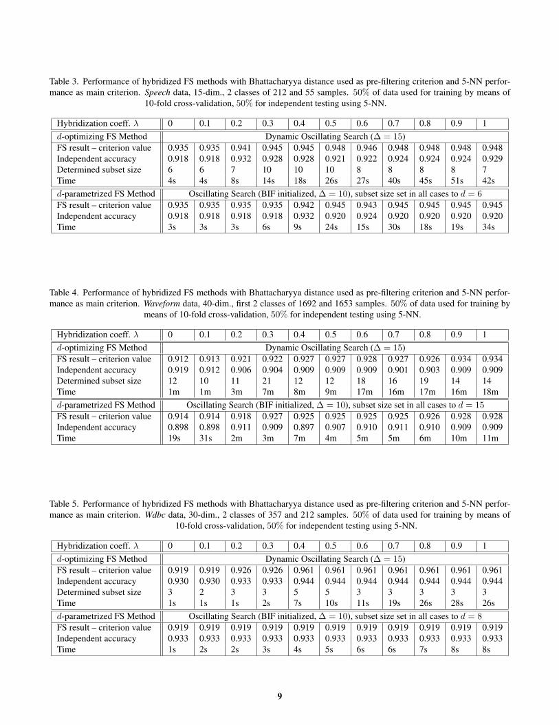
Table 3. Performance of hybridized FS methods with Bhattacharyya distance used as pre-filtering criterion and 5-NN perfor-mance as main criterion. Speech data, 15-dim., 2 classes of 212 and 55 samples. 50% of data used for training by means of

10-fold cross-validation, 50% for independent testing using 5-NN.

Hybridization coeff. λ 0 0.1 0.2 0.3 0.4 0.5 0.6 0.7 0.8 0.9 1d-optimizing FS Method Dynamic Oscillating Search (∆ = 15)FS result – criterion value 0.935 0.935 0.941 0.945 0.945 0.948 0.946 0.948 0.948 0.948 0.948Independent accuracy 0.918 0.918 0.932 0.928 0.928 0.921 0.922 0.924 0.924 0.924 0.929Determined subset size 6 6 7 10 10 10 8 8 8 8 7Time 4s 4s 8s 14s 18s 26s 27s 40s 45s 51s 42sd-parametrized FS Method Oscillating Search (BIF initialized, ∆ = 10), subset size set in all cases to d = 6FS result – criterion value 0.935 0.935 0.935 0.935 0.942 0.945 0.943 0.945 0.945 0.945 0.945Independent accuracy 0.918 0.918 0.918 0.918 0.932 0.920 0.924 0.920 0.920 0.920 0.920Time 3s 3s 3s 6s 9s 24s 15s 30s 18s 19s 34s

Table 4. Performance of hybridized FS methods with Bhattacharyya distance used as pre-filtering criterion and 5-NN perfor-mance as main criterion. Waveform data, 40-dim., first 2 classes of 1692 and 1653 samples. 50% of data used for training by

means of 10-fold cross-validation, 50% for independent testing using 5-NN.

Hybridization coeff. λ 0 0.1 0.2 0.3 0.4 0.5 0.6 0.7 0.8 0.9 1d-optimizing FS Method Dynamic Oscillating Search (∆ = 15)FS result – criterion value 0.912 0.913 0.921 0.922 0.927 0.927 0.928 0.927 0.926 0.934 0.934Independent accuracy 0.919 0.912 0.906 0.904 0.909 0.909 0.909 0.901 0.903 0.909 0.909Determined subset size 12 10 11 21 12 12 18 16 19 14 14Time 1m 1m 3m 7m 8m 9m 17m 16m 17m 16m 18md-parametrized FS Method Oscillating Search (BIF initialized, ∆ = 10), subset size set in all cases to d = 15FS result – criterion value 0.914 0.914 0.918 0.927 0.925 0.925 0.925 0.925 0.926 0.928 0.928Independent accuracy 0.898 0.898 0.911 0.909 0.897 0.907 0.910 0.911 0.910 0.909 0.909Time 19s 31s 2m 3m 7m 4m 5m 5m 6m 10m 11m

Table 5. Performance of hybridized FS methods with Bhattacharyya distance used as pre-filtering criterion and 5-NN perfor-mance as main criterion. Wdbc data, 30-dim., 2 classes of 357 and 212 samples. 50% of data used for training by means of

10-fold cross-validation, 50% for independent testing using 5-NN.

Hybridization coeff. λ 0 0.1 0.2 0.3 0.4 0.5 0.6 0.7 0.8 0.9 1d-optimizing FS Method Dynamic Oscillating Search (∆ = 15)FS result – criterion value 0.919 0.919 0.926 0.926 0.961 0.961 0.961 0.961 0.961 0.961 0.961Independent accuracy 0.930 0.930 0.933 0.933 0.944 0.944 0.944 0.944 0.944 0.944 0.944Determined subset size 3 2 3 3 5 5 3 3 3 3 3Time 1s 1s 1s 2s 7s 10s 11s 19s 26s 28s 26sd-parametrized FS Method Oscillating Search (BIF initialized, ∆ = 10), subset size set in all cases to d = 8FS result – criterion value 0.919 0.919 0.919 0.919 0.919 0.919 0.919 0.919 0.919 0.919 0.919Independent accuracy 0.933 0.933 0.933 0.933 0.933 0.933 0.933 0.933 0.933 0.933 0.933Time 1s 2s 2s 3s 4s 5s 6s 6s 7s 8s 8s

9

Springer-Verlag, 2006, 632–639.

[11] I. Guyon and A. Elisseeff, An introduction to variableand feature selection, J. Mach. Learn. Res., vol. 3, 1157–1182, 2003.

[12] I. Guyon, S. Gunn, M. Nikravesh, and L. Zadeh,Eds., Feature Extraction – Foundations and Applications,ser. Studies in Fuzziness and Soft Computing vol. 207.(Physica-Verlag, Springer, 2006).

[13] I. Kononenko, Estimating attributes: Analysis andextensions of relief, in ECML-94: Proc. European Conf. onMachine Learning. Secaucus, NJ, USA: Springer-VerlagNew York, Inc., 1994, 171–182.

[14] P. Pudil, J. Novovicova, N. Choakjarernwanit, andJ. Kittler, Feature selection based on approximation ofclass densities by finite mixtures of special type, PatternRecognition, vol. 28, 1389–1398, 1995.

[15] J. Novovicova, P. Pudil, and J. Kittler, Divergencebased feature selection for multimodal class densities,IEEE Trans. Pattern Anal. Mach. Intell., vol. 18, no. 2,218–223, 1996.

[16] P. A. Devijver and J. Kittler, Pattern Recognition: AStatistical Approach. (Englewood Cliffs, London, UK:Prentice Hall, 1982).

[17] P. Somol, P. Pudil, and J. Kittler, Fast branch & boundalgorithms for optimal feature selection, IEEE Trans-actions on Pattern Analysis and Machine Intelligence,vol. 26, no. 7, 900–912, 2004.

[18] S. Nakariyakul and D. P. Casasent, Adaptive branchand bound algorithm for selecting optimal features, PatternRecogn. Lett., vol. 28, no. 12, 1415–1427, 2007.

[19] F. Hussein, R. Ward, and N. Kharma, Geneticalgorithms for feature selection and weighting, a reviewand study, Proc. ICDAR, vol. 00, IEEE Comp. Soc.,1240–1244, 2001.

[20] H. Zhang and G. Sun, Feature selection using tabusearch method, Pattern Recognition, vol. 35, 701–711,2002.

[21] R. Jensen, Performing Feature Selection with ACO,ser. Studies in Computational Intelligence. SpringerBerlin / Heidelberg, 2006, vol. 34, 45–73.

[22] Y. Yang and J. O. Pedersen, A comparative study onfeature selection in text categorization, in ICML ’97: Proc.14th Int. Conf. on Machine Learning. San Francisco, CA,USA: Morgan Kaufmann Publishers Inc., 1997, 412–420.

[23] F. Sebastiani, Machine learning in automated textcategorization, ACM Computing Surveys, vol. 34, no. 1,1–47, March 2002.

[24] E. P. Xing, Feature Selection in Microarray Analysis.Springer, 2003, 110–129.

[25] Y. Saeys, I. naki Inza, and P. L. naga, A review offeature selection techniques in bioinformatics, Bioinfor-matics, vol. 23, no. 19, 2507–2517, 2007.

[26] R. Kohavi and G. H. John, Wrappers for feature subsetselection, Artif. Intell., vol. 97, no. 1-2, 273–324, 1997.

[27] A. W. Whitney, A direct method of nonparametricmeasurement selection, IEEE Trans. Comput., vol. 20,no. 9, 1100–1103, 1971.

[28] P. Pudil, J. Novovicova, and J. Kittler, Floating searchmethods in feature selection, Pattern Recogn. Lett., vol. 15,no. 11, 1119–1125, 1994.

[29] P. Somol, P. Pudil, J. Novovicova, and P. Paclık,Adaptive floating search methods in feature selection,Pattern Recogn. Lett., vol. 20, no. 11-13, 1157–1163,1999.

[30] S. Nakariyakul and D. P. Casasent, An improvementon floating search algorithms for feature subset selection,Pattern Recognition, vol. 42, no. 9, 1932–1940, 2009.

[31] P. Somol and P. Pudil, Oscillating search algorithmsfor feature selection, in ICPR 2000, vol. 02. Los Alami-tos, CA, USA: IEEE Computer Society, 2000, 406–409.

[32] J. Novovicova, P. Somol, and P. Pudil, Oscillatingfeature subset search algorithm for text categorization, inStructural, Syntactic, and Statistical Pattern Recognition,vol. LNCS 4109. Berlin / Heidelberg, Germany:Springer-Verlag, 2006, 578–587.

[33] A. Asuncion and D. Newman, UCI machine learningrepository, http://www.ics.uci.edu/ ∼mlearn/ mlreposi-tory.html, 2007.

[34] S. J. Raudys, Feature over-selection, in Structural,Syntactic, and Statistical Pattern Recognition, vol. LNCS4109. Berlin / Heidelberg, Germany: Springer-Verlag,2006, 622–631.

[35] P. Somol, J. Novovicova, J. Grim, and P. Pudil, Dy-namic oscillating search algorithms for feature selection,in ICPR 2008. Los Alamitos, CA, USA: IEEE ComputerSociety, 2008.

10