Feature Subset Selection by Bayesian networks: a comparison with genetic and sequential algorithms

Feature Subset Selection by Bayesiannetworks: a comparison with genetic andsequential algorithms1Department of Computer Science and Arti�cial Intelligence.University of the Basque Country.P.O. Box 649.E-20080 Donostia - San Sebasti�an.Basque Country.Spain.Telf: (+34) 943015026.Fax: (+34) 943219306.e-mail: [email protected]

1

AbstractIn this paper we perform a comparison among FSS-EBNA, a randomized, population-based and evolutionary algorithm, and two genetic and other two sequential search ap-proaches in the well known Feature Subset Selection (FSS) problem. In FSS-EBNA, theFSS problem, stated as a search problem, uses the EBNA (Estimation of Bayesian Net-work Algorithm) search engine, an algorithm within the EDA (Estimation of DistributionAlgorithm) approach. The EDA paradigm is born from the roots of the GA communityin order to explicitly discover the relationships among the features of the problem and notdisrupt them by genetic recombination operators. The EDA paradigm avoids the use ofrecombination operators and it guarantees the evolution of the population of solutions andthe discovery of these relationships by the factorization of the probability distribution ofbest individuals in each generation of the search. In EBNA, this factorization is carried outby a Bayesian network induced by a cheap local search mechanism. FSS-EBNA can be seenas an hybrid Soft Computing system, a synergistic combination of probabilistic and evolu-tionary computing to solve the FSS task. Promising results on a set of real Data Miningdomains are achieved by FSS-EBNA in the comparison respect to well known genetic andsequential search algorithms.Keywords: Feature Subset Selection, Estimation of Distribution Algorithm, Soft Computing,Estimation of Bayesian Network Algorithm, Bayesian network, predictive accuracy

2

I. MotivationThe basic problem of Supervised Classi�cation in Data Mining is concerned with the inductionof a model that classi�es a given object into one of several known classes. In order toinduce the classi�cation model, each object is described by a pattern of d features. Withadvanced computer technologies, big data archives are usually formed and many featuresare used to describe the objects. Here, Data Mining and Machine Learning communitiesusually formulate the following question: `Are all of these d descriptive features useful forlearning the classi�cation model?' On trying to respond to this question, we come up withthe Feature Subset Selection (FSS) approach, which can be reformulated as follows: given aset of candidate features, select the best subset in a classi�cation task.The dimensionality reduction made by a FSS process can carry out several advantages for aclassi�cation system in a speci�c task:� a reduction in the cost of adquisition of the data;� improvement of the comprensibility of the �nal classi�cation model;� a faster induction of the �nal classi�cation model;� an improvement in classi�cation accuracy.The attainment of higher classi�cation accuracies, coupled with a notable dimensionalityreduction, is the common objective of Machine Learning and Data Mining processes.It has long been proved that the classi�cation accuracy of supervised classi�ers is not mono-tonic with respect to the addition of features. Irrelevant or redundant features, depending onthe speci�c characteristics of the supervised classi�er, may degrade the predictive accuracyof the classi�cation model.FSS can be viewed as a search problem, with each state in the search space specifying asubset of the possible features of the task. Exhaustive evaluation of possible feature subsetsis usually unfeasible in practice because of the large amount of computational e�ort required.Due to its randomized, evolutionary and population-based nature, Genetic Algorithms (GAs)have been the most commonly used search engine in the FSS process (Kudo and Sklansky[32], Siedelecky and Sklansky [54], Vafaie and De Jong [58]). Most of the theory of GAsdeals with the so-called Building Blocks (BBs, Goldberg [18]); simply said, by BBs, partialsolutions of a problem are meant, formed by groups of related variables. GAs reproduceBBs by an implicit manipulation of a large number of them by mechanisms of selection and3

recombination. A crucial factor of the GA success resides in the proper growth and mixing ofthe optimal BBs of the problem. Problem-independent recombination operators often breakthese BBs and do not mix them e�ciently; thus, this could delay the discovery of the globaloptima or produce a convergence to a local optima.Linkage learning (LL) (Harik and Goldberg [20]) is the identi�cation of the BBs to be con-served under recombination. Recently, various approaches to solve the LL problem have beenproposed. Several proposed methods are based on the manipulation of the representation ofsolutions during the optimization to make the interacting components of partial solutions lesslikely to be broken. For this purpose, various reordering and mapping operators are used.One of these approaches is the well known Messy Genetic Algorithm (MGA) (Goldberg [18]).Instead of extending the GA, in latter years, a new approach has strongly emerged under theEDA term (Estimation of Ditribution Algorithm, M�uehlenbein and Paa�[43], Larra~naga andLozano [37]). EDA approach explicitly learns the probabilistic structure of the problem anduses this information to ensure a proper mixing and growth of BBs that do not disrupt them.The further exploration of the search space is guided, instead of crossover and mutationoperators as in GAs, by the probabilistic modeling of promising solutions.Bearing these di�culties in mind, in this paper we perform a comparison in the FSS taskamong FSS-EBNA [25], a novel algorithm inspired on the EDA approach, and other classicgenetic and sequential search algorithms. FSS-EBNA (Feature Subset Selection by Estima-tion of Bayesian Network Algorithm) is based on the probabilistic modeling by Bayesiannetworks (BNs) of promising solutions (feature subsets, in our case) to guide further explo-ration of the space of features. This BN is sampled to obtain the next generation of featuresubsets, therefore, guaranteeing the evolution of the search for the optimal subset of features.Using a wrapper approach to evaluate the goodness of each candidate feature subset, wesearch for the feature subset which maximizes the predictive accuracy of the Naive-Bayessupervised classi�er on presented tasks. However, this paper presents the �rst comparisonamong FSS-EBNA and other classic search algorithms in the FSS task.FSS-EBNA can be seen as an hybrid Soft Computing (Bonissone et al. [7]) system, a syn-ergistic combination of probabilistic and evolutionary computing to solve the FSS task: theuse of a classic probabilistic paradigm as Bayesian networks in conjunction with the evolu-tionary strategy scheme of the EDA paradigm, enables us to construct an application whichtackles the FSS problem. The remainder of the paper is organized as follows: the next sec-4

tion introduces the FSS problem and its basic components. Section 3 introduces the EDAapproach, BNs and the combination of both, the EBNA search engine. Section 4 presents theapplication of EBNA to the FSS problem, resulting in the FSS-EBNA algorithm. In section5, we compare it against four well known FSS methods, specially focusing our attention onthe comparison against two genetic approaches. The last section picks up the summary ofour work and some ideas about future lines of research.II. Feature Subset Selection as a search problemEven if we locate our work as a Machine Learning or Data Mining approach, the FSS liter-ature includes plenty of works in other �elds such as Pattern Recognition (Jain and Chan-drasekaran [27], Kittler [29]), Statistic (Miller [40], Narendra and Fukunaga [46]) or Text-Learning (Mladeni�c [41]). In the Bayesian network community we have the example of thework of Provan and Singh [51], who, using a Bayesian network as a classi�er, build it select-ing in a greedy manner the variables that should maximize the predictive accuracy of thenetwork. Thus, di�erent communities have exchanged and shared ideas among them to dealwith the FSS problem.As reported by Aha and Bankert [2], the objective of FSS in Machine Learning and DataMining is to reduce the number of features used to characterize a dataset so as to improvea classi�er's performance on a given task. In our framework we will appreciate a tradeo�between a high-predictive-accuracy and a low-cardinality (selection of few features) in the�nally chosen feature subset. The FSS task can be exposed as a search problem, each statein the search space identifying a subset of possible features.Thus, any FSS algorithm must determine four basic issues that de�ne the nature of the searchprocess (see Liu and Motoda [39] for a review of FSS algorithms):1. The starting point in the space. It determines the direction of the search. One mightstart with no features and successively add them, or one might start with all features andsuccessively remove them. One might also select an initial state somewhere in the middle ofthe search space.2. The organization of the search. It determines the strategy of the search. Roughly speak-ing, the search strategies can be complete or heuristic. The basis of the complete search isthe systematic examination of every possible feature subset. Three classic complete searchimplementations are depth-�rst, breadth-�rst and branch and bound search (Narendra and5

Fukunaga [46]). On the other hand, among heuristic algorithms, there are deterministicheuristic algorithms and non-deterministic heuristic ones. Classic deterministic heuristicFSS algorithms are sequential forward selection and sequential backward elimination (Kittler[29]), oating selection methods (Pudil et al. [52]) and best-�rst search (Kohavi and John[30]). They are deterministic in the sense that all the runs always obtain the same solution.Non-deterministic heuristic search is used to escape from local maximums. Randomness isused for this purpose and this implies that one should not expect the same solution fromdi�erent runs. Two classic implementations of non-deterministic search engines are the fre-quently applied Genetic Algorithms (Siedelecky and Sklansky [54]) and Simulated Annealing(Doak [15]).3. Evaluation strategy of feature subsets. By the calculation of the goodness of each proposedfeature subset the evaluation function identi�es the promising areas of the search space.The objective of FSS algorithm is its maximization. The search algorithm uses the valuereturned by the evaluation function to guide the search. Some evaluation functions carryout this objective looking only at the intrinsic characteristics of the data and measuringthe power of a feature subset to discriminate among the classes of the problem: this typeof evaluation functions are grouped below the �lter strategy. These evaluation functionsare usually monotonic and increase with the addition of features that afterwards can hurtthe predictive accuracy of the �nal classi�er. However, Kohavi and John [30] reported thatwhen the goal of FSS is the maximization of the accuracy, the features selected shoulddepend not only on the features and the target concept to be learned, but also on the specialcharacteristics of the supervised classi�er. Thus, they proposed the wrapper concept: thisimplies that the FSS algorithm conducts the search for a good subset using the classi�er itselfas a part of the evaluation function, the same classi�er that will be used to induce the �nalclassi�cation model. Once the classi�cation algorithm is �xed, the idea is to train it withthe feature subset found by the search algorithm, estimating the predictive accuracy on thetraining set and assigning it as the value of the evaluation function of the feature subset.4. Criterion for halting the search. An intuitive approach for stopping the search will bethe non-improvement of the evaluation function value of alternative subsets. Another classiccriterion will be to �x an amount of possible solutions to be visited along the search.6

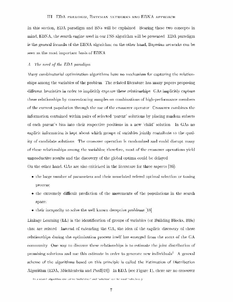
III. EDA paradigm, Bayesian networks and EBNA approachIn this section, EDA paradigm and BNs will be explained. Bearing these two concepts inmind, EBNA, the search engine used in our FSS algorithm will be presented. EDA paradigmis the general formula of the EBNA algorithm; on the other hand, Bayesian networks can beseen as the most important basis of EBNA.A. The need of the EDA paradigmMany combinatorial optimization algorithms have no mechanism for capturing the relation-ships among the variables of the problem. The related literature has many papers proposingdi�erent heuristics in order to implicitly capture these relationships. GAs implicitly capturethese relationships by concentrating samples on combinations of high-performance membersof the current population through the use of the crossover operator. Crossover combines theinformation contained within pairs of selected `parent' solutions by placing random subsetsof each parent's bits into their respective positions in a new `child' solution. In GAs noexplicit information is kept about which groups of variables jointly contribute to the qual-ity of candidate solutions. The crossover operation is randomized and could disrupt manyof these relationships among the variables; therefore, most of the crossover operations yieldunproductive results and the discovery of the global optima could be delayed.On the other hand, GAs are also criticized in the literature for three aspects [36]:� the large number of parameters and their associated refered optimal selection or tuningprocess;� the extremely di�cult prediction of the movements of the populations in the searchspace;� their incapacity to solve the well known deceptive problems [18].Linkage Learning (LL) is the identi�cation of groups of variables (or Building Blocks, BBs)that are related. Instead of extending the GA, the idea of the explicit discovery of theserelationships during the optimization process itself has emerged from the roots of the GAcommunity. One way to discover these relationships is to estimate the joint distribution ofpromising solutions and use this estimate in order to generate new individuals1. A generalscheme of the algorithms based on this principle is called the Estimation of DistributionAlgorithm (EDA, M�uehlenbein and Paa�[43]). In EDA (see Figure 1), there are no crossover1In a search algorithm the terms `individual' and `solution' can be used indistinctly.7

1. D0 Generate N individuals (the initial population) randomly.2. Repeat for l = 1; 2; : : : until a stop criterion is met:2.1. Dsl�1 Select S � N individuals from Dl�1 according to a selection method.2.2. pl(x) = p(xjDsl�1) Estimate the joint probability distribution of an individual beingamong the selected inviduals.2.3. Dl Sample N individuals (the new population) from pl(x).Fig. 1. Main scheme of the EDA paradigm.nor mutation operators, and the new population is sampled from a probability distributionwhich is estimated from the selected individuals. However, estimating the distribution is acritical task in EDA (for a more complete review see Larra~naga et al. [36]).The simplest way to estimate the distribution of good solutions assumes the independencebetween the features2 of the problem. New candidate solutions are sampled by only regardingthe proportions of the values of the variables independently to the remaining ones. PopulationBased Incremental Learning (PBIL, Baluja [5]), Compact Genetic Algorithm (cGA, Harik etal. [20]), Univariate Marginal Distribution Algorithm (UMDA, M�uehlenbein [42]) and Bit-Based Simulated Crossover (BSC, Syswerda [57]) are four algorithms of this type. They workwell in problems with no signi�cant interactions (or relationships) among features and so,the need for covering higher order interactions among the variables is seen for more complexor real tasks.E�orts covering pairwise interactions among the features of the problem have generatedalgorithms such as: MIMIC uses simple chain distributions (De Bonet et al. [14]), the so-called dependency trees (Baluja and Davies [6]) and the Bivariate Marginal DistributionAlgorithm (BMDA, Pelikan and M�uehlenbein [50]). However, Pelikan and M�uehlenbein [50]have demonstrated that only covering pairwise dependencies is not enough with problemswhich have higher order interactions: in this type of problems the discovery of the globaloptimum is considerably delayed when lower order based probability estimating approachesare used.In this way, the Factorized Distribution Algorithm (FDA, M�uehlenbein and Mahnig [44])covers higher order interactions. This is done using a previously �xed factorization of the2In the Evolutionary Computation community, the term `variable' is normally used instead of `feature'. We use both termsindistinctly. 8

joint probability distribution. However, FDA needs prior information on the decompositionand factorization of the problem which is often not available. Without the need of this extrainformation about the decomposition and factorization of the problem, other probabilisticmodels, able to cover higher order interactions, appear in the literature. For this purpose,Bayesian networks, graphical representations able to cover these higher order interactions,can be used. Thus, EBNA (Etxeberria and Larra~naga [16]) BOA (Pelikan et al. [49]) arealgorithms which use di�erent implementations of Bayesian networks for estimating the jointdistribution of promising solutions. In this way, multivariate interactions among variablescan be covered. In Soto et al. [56] a Bayesian network with a polytree structure is proposed:the proposed algorithm is called PADA (Polytree Approximation of Ditribution Algorithms)and it is based on a method proposed by Acid and de Campos [1] for detecting relationshipsamong variables. Ochoa et al. [47] propose an initial algorithm to learn (from conditionalindependence tests) the junction tree from a database. Harik presents an algorithm (Extendcompact Genetic Algorithm, EcGA [21]), whose basic idea consists of factorizing the jointprobability distribution in a product of marginal distributions of variable size: these marginaldistributions of variable size are related to the variables that are contained in the same groupand to the probability distributions associated to them.Many of these works notify of a faster discovery of the global optimum by EDA algorithmsthan GAs for certain combinatorial optimization problems. Harik [21] and Pelikan andM�uehlenbein [50] show several intuitive and well known problems where the GAs, whenthe crossover operator is applied, frequently disrupt optimum relationships among features:in this way, these optimum relationships that appear in the parent solutions will disappear inthe children solutions and the discovery of the global optimum will be delayed. Thus, theseauthors note that EDA approaches are able to �rst discover and then maintain these rela-tionships during the entire optimization process, producing a faster discovery of the globaloptimum than GAs.In order to avoid the evaluation of larger amounts of possible solutions (and its associatedCPU time), a faster discovery of well �tted areas in the search space is highly desired inthe FSS problem. Bearing this purpose in mind, we use an EDA inspired approach for FSS.Based on the EBNA work of Etxeberria and Larra~naga [16], we propose the use of Bayesiannetworks as the models for representing the probability distribution of the set of candidatesolutions for the FSS problem, using the application of automatic learning methods to induce9

the right distribution model in each generation in an e�cient way.B. Bayesian networksA Bayesian network (BN, Castillo et al. [9], Lauritzen [38], Pearl [48]) encodes the rela-tionships contained in the modelled data. It can be used to describe the data as well asto generate new instances of the variables with similar properties as those of given data.A Bayesian network encodes the probability distribution p(x), where X = (X1; :::;Xd) isa vector of variables, and it can be seen as a pair (M ,�). M is a directed acyclic graph(DAG) where the nodes correspond to the variables and the arcs represent the conditional(in)dependencies3 (Dawid [13]) among the variables. By Xi, both the variable and the nodecorresponding to this variable is denoted. M will give the factorization of p(x):p(x) = dYi=1 p(xij�i)where �i is the set of parent variables (nodes) that Xi has in M and �i its possible instan-tations. The number of states of �i will be denoted as j�ij = qi and the number of di�erentvalues of Xi as jXij = ri. � = f�ijkg are the required conditional probability values to com-pletely de�ne the joint probability distribution of X. �ijk will represent the probability ofXi being in its kth state while �i is in its jth instantation. This factorization of the jointdistribution can be used to generate new instances using the conditional probabilities in amodeled dataset.Informally, an arc between two nodes relates these nodes so that the value of the variablecorresponding to the ending node of the arc depends on the value of the variable correspondingto the starting node. Every probability distribution can be de�ned by a Bayesian network(Pearl [48]). As a result, Bayesian networks are widely used in problems where uncertaintyis handled using probabilities.Unfortunately, �nding the optimal M̂ requires searching through all possible structures, whichhas been proven to be NP-hard (Chickering et al. [11]). Although promising results havebeen obtained using global search techniques (Chickering et al. [12], Larra~naga et al. [34],Larra~naga et al. [35], Wong et al. [59]) their computation cost makes them unfeasible for ourproblem. We need to �nd M̂ as fast as possible, so a simple algorithm which returns a goodstructure, even if it is not optimal, will be preferred.3Let Y;Z and W be three disjoint sets of variables, then Y is said to be conditionally independent of Z given W, if andonly if p(y j z;w) = p(y j w), for all possible values y; z and w of Y;Z and W.10

In our implementation Algorithm B (Buntine [8]) is used for learning Bayesian networks fromdata. Algorithm B is a greedy search heuristic. The algorithm starts with an arc-less structurein each generation of the search and at each step, it adds the arc with the maximum increasein the BIC approximation (Penalized maximum likelihood of the proposed structure, Schwarz[55]). The algorithm stops when adding an arc does not increase the utilized measure. In theBIC metric, the penalized function is given by the Je�reys{Schwarz criterion, resulting in theBayesian Information Criterion (BIC [55]). The BIC score of a Bayesian network structureM , from a database D and containing N cases (characterised by d variables) is denoted asfollows: BIC(M;D) = dXi=1 qiXj=1 riXk=1Nijk log NijkNij � logN2 dXi=1(ri � 1)qiNijk denotes the number of cases in D in which the variable Xi is instantiated to its k-thvalue and its parents in the network structure are instantiated to their j-th value. Let beNij =Prik=1Nijk, where ri and qi represent the number of possible states of Xi and its parentsrespectively.C. Estimation of Bayesian Network Algorithm: EBNAThe general procedure of EBNA appears in Figure 2. To understand the steps of the algo-rithm, the following concepts must be clari�ed.M0 is the DAG with no arcs at all and �0= f8i : p(Xi = xi) = 1ri g, which means thatthe initial Bayesian network BN0, assigns the same probability to all individuals. N is thenumber of individuals in the population. S is the number of individuals selected from thepopulation. Although S can be any value, the most common value in the EDA literature isS = N2 . If S is close to N then the populations will not evolve very much from generationto generation. On the other hand, a low S value will lead to low diversity resulting in earlyconvergence.For individual selection range based selection is proposed, i.e., selecting the best N=2 in-dividuals from the N individuals of the population. However, any selection method couldbe used. Probabilistic Logic Sampling algorithm (PLS, Henrion [22]) is used to sample newindividuals from the Bayesian network.Finally, the way in which the new population is created must be pointed out. In the givenprocedure, all individuals from the previous population are discarded and the new popula-11

1. BN0 (M0,�0).2. D0 Sample N individuals from BN0.3. For l = 1; 2; : : : until a stop criterion is met:3.1. Dsl�1 Select S individuals from Dl�1.3.2. M̂l Find the structure which maximizes BIC(Ml;Dsl�1).3.3. �l Calculate f�lijk = N l�1ijk +1N l�1ij +ri g using Dsl�1 as the data set.3.4. BNl (M̂l,�0).3.5. Dl Sample N individuals from BNl using PLS.Fig. 2. EBNA basic scheme.tion is composed of all newly created individuals4. This has the problem of losing the bestindividuals that have been previously generated, therefore, the following minor change hasbeen made: instead of discarding all the individuals, we maintain the best individual of theprevious generation and create N � 1 new individuals.An elitist approach is used to form iterative populations. Instead of directly discarding theN � 1 individuals from the previous generation replacing them with N � 1 newly generatedones, the 2N � 1 individuals are put together and the best N � 1 taken among them. Thesebest N � 1 individuals form the new population together with the best individual of theprevious generation. In this way, the populations converge faster to the best individualsfound; however, this also implies a risk of losing diversity within the population.The stopping criteria will be explained in the next section.IV. Feature Subset Selection by Estimation of Bayesian NetworkAlgorithm: FSS-EBNA. Instantation of FSS componentsOnce the FSS problem and EBNA algorithm are presented, we will use the search engineprovided by EBNA to solve the FSS problem, resulting in the FSS-EBNA algorithm. In thenext lines we will brie y describe its basic components (see Inza et al. [25] for more details).Parametrizing the FSS task as an optimization problem, it consists on selecting, for a trainingset characterised by d features, the subset of features which maximizes the accuracy of acertain classi�er on further test instances. Thus, the cardinality of the search space is 2d.Using an intuitive notation to represent each individual (there are d bits in each individual,4Newly created individuals are also known as `o�spring'. 12

1 0 0 ................... 0 ef10 0 1 ................... 1 ef21 1 1 ................... 0 ef30 1 1 ................... 1 ef4................................... .....1 0 1 ................... 1 efN

1234..N

selection of N/2

individuals

1 0 1 1 ................. 1 2 1 1 0 ................. 0 ... ................................ N/2 0 0 1 ................. 1

induction of the Bayesian networkwith ’d’ nodes

...................

sample ’N-1’ individuals from the Bayesian network and calculate their evaluation function values1 0 0 .................... 1 ef1

0 0 1 .................... 0 ef21 1 1 .................... 0 ef3.................................. .....0 1 1 .................... 1 efN-1

123..N-1

(2)

(4)

(5)

(6)

(7)

put together individuals from the previousgeneration (1) and newly generated ones (7), and take the best ’N-1’ of them to form the

next population (1)

(*) value of the evaluation function of the individual

(1)

(3) X X X X

X X X X

X X X X

1X

5X

dX

3X

8X

1 2 3 .............. d

1 2 3 ............. d

(*)

(*)1 2 3 .............. d

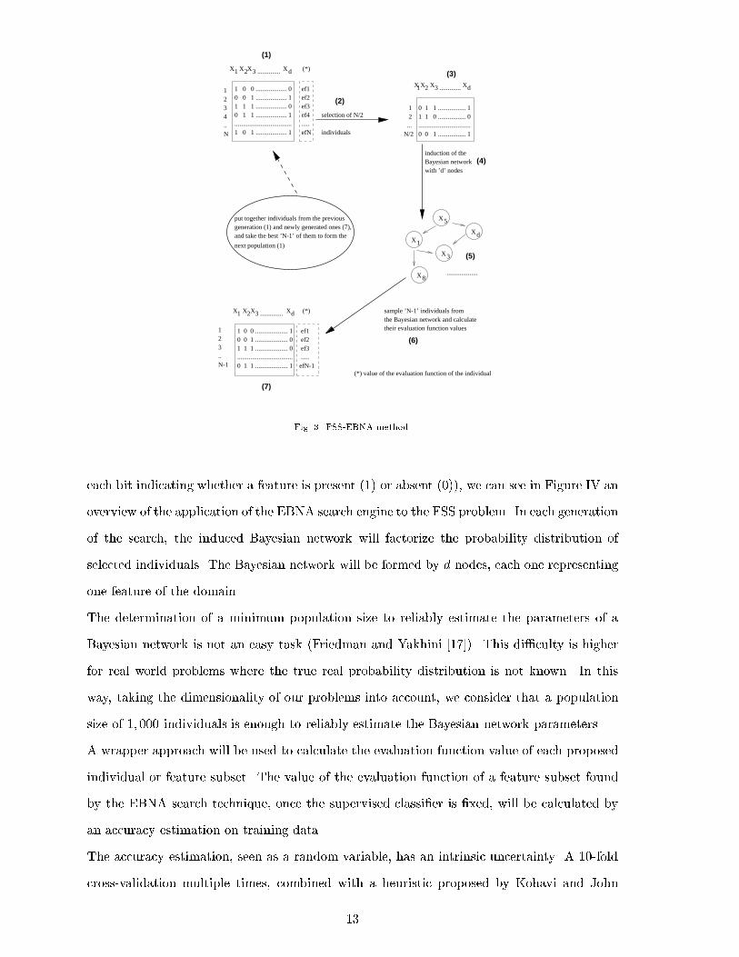
Fig. 3. FSS-EBNA method.each bit indicating whether a feature is present (1) or absent (0)), we can see in Figure IV anoverview of the application of the EBNA search engine to the FSS problem. In each generationof the search, the induced Bayesian network will factorize the probability distribution ofselected individuals. The Bayesian network will be formed by d nodes, each one representingone feature of the domain.The determination of a minimum population size to reliably estimate the parameters of aBayesian network is not an easy task (Friedman and Yakhini [17]). This di�culty is higherfor real world problems where the true real probability distribution is not known. In thisway, taking the dimensionality of our problems into account, we consider that a populationsize of 1; 000 individuals is enough to reliably estimate the Bayesian network parameters.A wrapper approach will be used to calculate the evaluation function value of each proposedindividual or feature subset. The value of the evaluation function of a feature subset foundby the EBNA search technique, once the supervised classi�er is �xed, will be calculated byan accuracy estimation on training data.The accuracy estimation, seen as a random variable, has an intrinsic uncertainty. A 10-foldcross-validation multiple times, combined with a heuristic proposed by Kohavi and John13

[30], will be used to control the intrinsic uncertainty of the evaluation function. The heuristicworks as follows:� if the standard deviation of the accuracy estimate is above 1%, another 10-fold cross-validation is executed;� this is repeated until the standard deviation drops below 1%, a maximum of �ve times.In this way, small datasets will be cross-validated many times. However, larger ones possiblyonce.Although FSS-EBNA is independent from the speci�c supervised classi�er used within itswrapper approach, in our set of experiments we will use the well known Naive-Bayes (NB,Cestnik [10]) supervised classi�er. It is a simple and fast classi�er which uses the Bayesrule to predict the class for each test instance, assuming that features are independent toeach other given the class. Due to its simplicity and fast induction, it is commonly usedon Data Mining tasks of high dimensionality (Kohavi and John [30], Mladeni�c [41]). Theprobability for discrete features is estimated from data using maximum likelihood estima-tion and applying the Laplace correction. A normal distribution is assumed to estimate theclass conditional probabilities for continuous attributes. Unknown values in the test instanceare skipped. Although its simplicity and its independence assumption among variables, theliterature shows that the NB classi�er gives remarkably high accuracies in many domains(Langley and Sage [33]), specially in medical ones. Despite its good scaling with irrelevantfeatures, NB can improve its accuracy level discarding correlated or redundant features. NB,based on the independence assumption of features to predict the class, is hurt by correlatedfeatures which violate this independence assumption. Thus, FSS can also play a `normaliza-tion' role to discard these groups of correlated features, ideally selecting one of them in the�nal model. Although Langley and Sage [33] propose a sequential forward feature selectionfor detecting these correlations (starting from an empty subset of features and sequentiallyselecting features until no improvement is achieved), Kohavi and John [30] prefer a sequentialbackward elimination (starting from the full set of features and sequentially deleting featuresuntil no improvement is achieved). In our work we propose the use of FSS-EBNA to detectthese redundancies among features to improve NB's predictive accuracy.To stop the search algorithm, we have adopted an intuitive stopping criteria which takesthe number of instances of the training set into account. In this way, we try to avoid the14

`over�tting' risk (Jain and Zongker [28], Kohavi and John [30]):� for datasets with more than 2; 000 instances, the search is stopped when in a samplednew generation no feature subset appears with an evaluation function value improvingthe best subset found in the previous generation. Thus, the best subset of the search,found in the previous generation, is returned as the FSS-EBNA's solution;� for smaller datasets the search is stopped when in a sampled new generation no featuresubset appears with an evaluation function value improving, at least with a p-valuesmaller than 0:15, the value of the evaluation function of the best feature subset of theprevious generation. Thus, the best subset of the previous generation is returned as theFSS-EBNA's solution.For larger datasets the `over�tting' phenomenom has a lesser impact and we hypothesize thatan improvement in the accuracy estimation over the training set will be coupled with an im-provement in generalization accuracy on unseen instances. Otherwise, for smaller datasets, inorder to avoid the `over�tting' risk, the continuation of the search is only allowed when a sig-ni�cant improvement in the accuracy estimation of best individuals of consecutive generationsappears. We hypothesize that when this signi�cant improvement appears, the `over�tting'risk decays and there is a basis for further generalization accuracy improvement over unseeninstances.Another concept to understand this stopping criteria is the wrapper nature of the proposedevaluation function. As we will see in the next section, the evaluation function value of eachvisited solution (the accuracy estimation of the NB classi�er on training set by 10-fold cross-validation multiple times, using only the features proposed by the solution) needs severalseconds to be calculated (never more than 4 seconds for used datasets). As the generationof a new generation of individuals implies the evaluation of 1; 000 new individuals, we onlyallow the continuation of the search when it demonstrates that it is able to escape fromthe local optimas, being able to discover new `best' solutions in each generation. When thewrapper approach is used, the CPU time must be also controled: we hypothesize that whenthe continuation of the search is allowed by our stopping criteria, the CPU times to evaluatea new generation of solutions are justi�ed. For a larger study about this stopping criterion,the work [25] can be consulted.5Using a 10-fold cross-validated paired t test between the folds of both estimations, taking only the �rst run into accountwhen 10-fold cross-validation is repeated multiple times. 15

Table I. Details of experimental domains. C = continuous. D = discrete.domain number of instances number of classes number of features and their typesIonosphere 351 2 34 (34-C)Horse-colic 368 2 22 (15-D, 7-C)Soybean-large 683 19 35 (35-C)Anneal 898 6 38 (6-D, 32-C)Image 2,310 7 19 (19-C)V. Empirical comparisonWe will test the power of FSS-EBNA in �ve real datasets. Table 1 re ects the principalcharacteristics of the datasets. All datasets come from the UCI repository (Murphy [45]) andthey have been frequently used in the FSS literature. Due to their large dimensionality, anexhaustive search for the best feature subset is not computationally feasible, so a heuristicsearch must be performed.In real datasets we do not know the optimal subset of features respect to the Naive-Bayesclassi�er. To test the power of FSS-EBNA, a comparison with the following well known FSSalgorithms is carried out:� Sequential Forward Selection (SFS) is a classic hill-climbing search algorithm (Kittler[29]) which starts from an empty subset of features and sequentially selects features untilno improvement is achieved in the evaluation function value. It performs the major partof its search near the empty feature set;� Sequential Backward Elimination (SBE) is another classic hill-climbing algorithm (Kit-tler [29]) which starts from the full set of features and sequentially deletes features untilno improvement is achieved in the evaluation function value. It performs the major partof its search near the full feature set. Instead of working with a population of solutions,SFS and SBE try to optimize a single feature subset;� GA with one-point crossover (GA-o);� GA with uniform crossover (GA-u);� FSS-EBNA.For all the FSS algorithms, the wrapper evaluation function explained in the previous sectionis used. Although SFS and SBE algorithms stop deterministically, GA algorithms apply thesame stopping criteria as FSS-EBNA.Although the optimal selection of parameters is still an open problem on GAs (Grefenstatte16

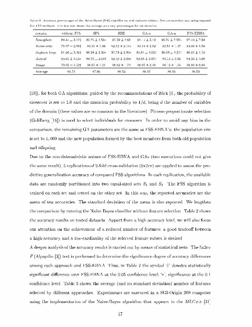
Table II. Accuracy percentages of the Naive-Bayes (NB) classi�er on real datasets without feature selection and using exposed�ve FSS methods. The last row shows the average accuracy percentages for six domains.domain without FSS SFS SBE GA-o GA-u FSS-EBNAIonosphere 84:84� 3:12y 90:25 � 1:58� 91:39 � 2:68 91:17� 3:19 90:97 � 2:56� 92:40� 2:04Horse-colic 78:97� 2:98y 83:31� 1:98 82:12� 2:41� 83:43� 2:82 83:51� 1:47 83:93� 1:58Soybean-large 81:96� 3:46y 86:38 � 3:30� 87:78� 3:90� 85:64� 4:06y 86:09 � 4:37y 88:64� 1:70Anneal 93:01� 3:13� 86:72 � 2:09y 92:49� 2:94� 92:95� 2:67� 93:13� 2:56 94:10� 3:00Image 79:95� 1:52y 88:65� 1:21 88:82 � 1:74 88:67� 2:48 89:12� 1:56 88:98� 0:98Average 83:74 87:06 88:52 88:37 88:56 89:53[19]), for both GA algorithms, guided by the recommendations of B�ack [4], the probability ofcrossover is set to 1:0 and the mutation probability to 1=d, being d the number of variablesof the domain (these values are so common in the literature). Fitness-proportionate selection(Goldberg [18]) is used to select individuals for crossover. In order to avoid any bias in thecomparison, the remaining GA parameters are the same as FSS-EBNA's: the population sizeis set to 1; 000 and the new population formed by the best members from both old populationand o�spring.Due to the non-deterministic nature of FSS-EBNA and GAs (two executions could not givethe same result), 5 replications of 2-fold cross-validation (5x2cv) are applied to assess the pre-dictive generalization accuracy of compared FSS algorithms. In each replication, the availabledata are randomly partitioned into two equal-sized sets S1 and S2. The FSS algorithm istrained on each set and tested on the other set. In this way, the reported accuracies are themean of ten accuracies. The standard deviation of the mean is also reported. We lengthenthe comparison by running the Naive-Bayes classi�er without feature selection. Table 2 showsthe accuracy results on tested datasets. Appart from a high accuracy level, we will also focusour attention on the achievement of a reduced number of features: a good tradeo� betweena high-accuracy and a low-cardinality of the selected feature subset is desired.A deeper analysis of the accuracy results is carried out by means of statistical tests. The 5x2cvF (Alpaydin [3]) test is performed to determine the signi�cance degree of accuracy di�erencesamong each approach and FSS-EBNA. Thus, in Table 2 the symbol `y' denotes statisticallysigni�cant di�erence over FSS-EBNA at the 0:05 con�dence level; `�', signi�cance at the 0:1con�dence level. Table 3 shows the average (and its standard deviation) number of featuresselected by di�erent approaches. Experiments are executed in a SGI-Origin 200 computerusing the implementation of the Naive-Bayes algorithm that appears in the MLC++ [31]17

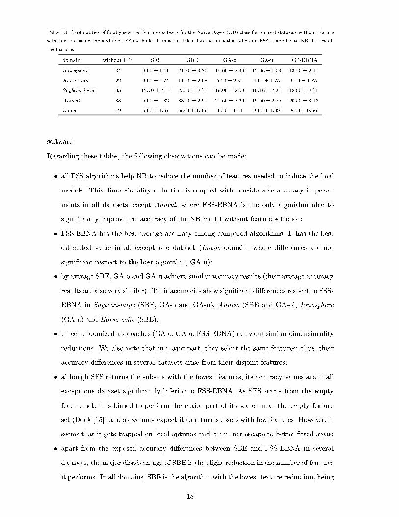
Table III. Cardinalities of �nally selected features subsets for the Naive-Bayes (NB) classi�er on real datasets without featureselection and using exposed �ve FSS methods. It must be taken into account that when no FSS is applied to NB, it uses allthe features.domain without FSS SFS SBE GA-o GA-u FSS-EBNAIonosphere 34 6:00� 1:41 21:30� 3:80 15:00� 2:36 12:66� 1:03 13:40� 2:11Horse-colic 22 6:00� 2:74 11:20� 2:65 5:00 � 2:82 4:60 � 1:75 6:10� 1:85Soybean-large 35 12:70� 2:71 23:50� 2:75 19:00� 2:09 19:16� 2:31 18:90� 2:76Anneal 38 5:50� 2:32 33:60� 2:91 21:66� 2:66 19:50� 2:25 20:50� 3:13Image 19 5:60� 1:57 9:40� 1:95 8:00 � 1:41 8:00 � 1:09 8:00� 0:66software.Regarding these tables, the following observations can be made:� all FSS algorithms help NB to reduce the number of features needed to induce the �nalmodels. This dimensionality reduction is coupled with considerable accuracy improve-ments in all datasets except Anneal, where FSS-EBNA is the only algorithm able tosigni�cantly improve the accuracy of the NB model without feature selection;� FSS-EBNA has the best average accuracy among compared algorithms. It has the bestestimated value in all except one dataset (Image domain, where di�erences are notsigni�cant respect to the best algorithm, GA-u);� by average SBE, GA-o and GA-u achieve similar accuracy results (their average accuracyresults are also very similar). Their accuracies show signi�cant di�erences respect to FSS-EBNA in Soybean-large (SBE, GA-o and GA-u), Anneal (SBE and GA-o), Ionosphere(GA-u) and Horse-colic (SBE);� three randomized approaches (GA-o, GA-u, FSS-EBNA) carry out similar dimensionalityreductions. We also note that in major part, they select the same features: thus, theiraccuracy di�erences in several datasets arise from their disjoint features;� although SFS returns the subsets with the fewest features, its accuracy values are in allexcept one dataset signi�cantly inferior to FSS-EBNA. As SFS starts from the emptyfeature set, it is biased to perform the major part of its search near the empty featureset (Doak [15]) and as we may expect it to return subsets with few features. However, itseems that it gets trapped on local optimas and it can not escape to better �tted areas;� apart from the exposed accuracy di�erences between SBE and FSS-EBNA in severaldatasets, the major disadvantage of SBE is the slight reduction in the number of featuresit performs. In all domains, SBE is the algorithm with the lowest feature reduction, being18

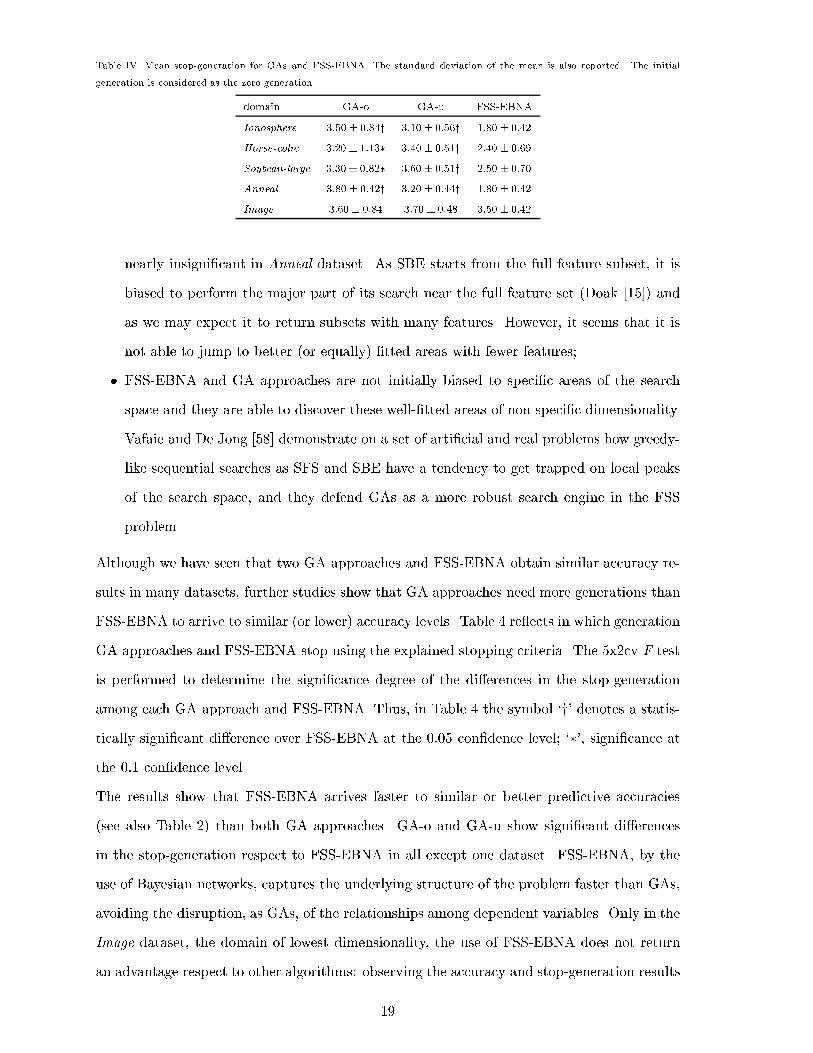
Table IV. Mean stop-generation for GAs and FSS-EBNA. The standard deviation of the mean is also reported. The initialgeneration is considered as the zero generation.domain GA-o GA-u FSS-EBNAIonosphere 3:50� 0:84y 3:10� 0:56y 1:80� 0:42Horse-colic 3:20� 1:13� 3:40� 0:51y 2:40� 0:69Soybean-large 3:30� 0:82� 3:60� 0:51y 2:50� 0:70Anneal 3:80� 0:42y 3:20� 0:44y 1:80� 0:42Image 3:60� 0:84 3:70 � 0:48 3:50� 0:42nearly insigni�cant in Anneal dataset. As SBE starts from the full feature subset, it isbiased to perform the major part of its search near the full feature set (Doak [15]) andas we may expect it to return subsets with many features. However, it seems that it isnot able to jump to better (or equally) �tted areas with fewer features;� FSS-EBNA and GA approaches are not initially biased to speci�c areas of the searchspace and they are able to discover these well-�tted areas of non speci�c dimensionality.Vafaie and De Jong [58] demonstrate on a set of arti�cial and real problems how greedy-like sequential searches as SFS and SBE have a tendency to get trapped on local peaksof the search space, and they defend GAs as a more robust search engine in the FSSproblem.Although we have seen that two GA approaches and FSS-EBNA obtain similar accuracy re-sults in many datasets, further studies show that GA approaches need more generations thanFSS-EBNA to arrive to similar (or lower) accuracy levels. Table 4 re ects in which generationGA approaches and FSS-EBNA stop using the explained stopping criteria. The 5x2cv F testis performed to determine the signi�cance degree of the di�erences in the stop-generationamong each GA approach and FSS-EBNA. Thus, in Table 4 the symbol `y' denotes a statis-tically signi�cant di�erence over FSS-EBNA at the 0:05 con�dence level; `�', signi�cance atthe 0:1 con�dence level.The results show that FSS-EBNA arrives faster to similar or better predictive accuracies(see also Table 2) than both GA approaches. GA-o and GA-u show signi�cant di�erencesin the stop-generation respect to FSS-EBNA in all except one dataset. FSS-EBNA, by theuse of Bayesian networks, captures the underlying structure of the problem faster than GAs,avoiding the disruption, as GAs, of the relationships among dependent variables. Only in theImage dataset, the domain of lowest dimensionality, the use of FSS-EBNA does not returnan advantage respect to other algorithms: observing the accuracy and stop-generation results19

in this domain, all FSS algorithms demonstrate a similar behaviour, �nding similarly-�ttedsubsets and population-based approaches needing nearly the same number of generations tostop.This faster discovery of optimal solutions by EDA approaches than GAs was also noted byHarik [21] and Pelikan and M�uehlenbein [50] in a set of classical optimization problems. As inour case, when a wrapper approach is used to calculate the evaluation function value of eachfound subset, the faster discovery of similar or better accuracies is a critical task. AlthoughNB is a fast supervised classi�er, it needs several seconds to estimate the predictive accuracy(by the exposed 10-fold cross-validation multiple times) of a feature subset on the training set:depending on the number of features selected by the subset, near 1 CPU second is neededin Ionosphere (the domain with fewest instances), while near 3 are needed in Image (thedomain with most instances). As the generation of a new population of solutions implies theevaluation of new 1; 000 individuals, an earlier stop without a damage to the accuracy levelis highly desired in order to save CPU time. On the other hand, the times for the inductionof the Bayesian networks over the best individuals are insigni�cant in all domains: 3 CPUseconds are needed by average in Image domain (the domain with fewer features) and 14CPU seconds in Anneal (the domain with more features).In a subsequent analysis between GA-o and GA-u predictive accuracies, we note that thedi�erences are not statistically signi�cant in any dataset. So, we should focus our attentionon their stop-generation numbers to extract di�erences between the behaviour of GA-o andGA-u. Thus, observing Table 4, the one-point crossover is better suited for Horse-colic andSoybean-large datasets than the uniform crossover; otherwise, we see the opposite behaviourin Ionosphere and Anneal. By the use of FSS-EBNA, we also avoid this tunning amongdi�erent crossover operators for each dataset.VI. Summary and future workIn this work, we have performed a comparison among FSS-EBNA, a randomized and population-based evolutionary algorithm, and two genetic and other two sequential classic search algo-rithms in the FSS task. In FSS-EBNA, the FSS problem, stated as a search problem, usesthe EBNA (Estimation of Bayesian Network Algorithm) search engine, a variant of the EDA(Estimation of Distribution Algorithm) approach. The EDA paradigm is born from the rootsof the GA community in order to explicitly discover the relationships among the features of20

the problem and not disrupt them by genetic recombination operators. The EDA paradigmavoids the use of recombination operators and it guarantees the evolution of solutions andthe discovery of these relationships by the factorization of the probability distribution of bestindividuals in each generation of the search. In EBNA, this factorization is carried out by aBayesian network induced by a cheap local search mechanism. As another attractive e�ect,with the use of FSS-EBNA we avoid the tuning of genetic parameters, still an open problemon GA literature.Using a wrapper approach, we have searched for the subset of features that optimizes thepredictive accuracy of the Naive-Bayes supervised classi�er. We have carried out a comparisonin a set of tasks among two well known sequential search engines algorithms (SequentialForward Selection and Sequential Backward Elimination) and Genetic Algorithms with one-point and uniform crossover operators. FSS-EBNA has demonstrated a robust behaviour,obtaining the best average accuracy respect to all the tasks, the best in all except one datasetand a large reduction in the number of selected features respect the full feature set. We havenoted the tendency of Sequential Forward Selection to get trapped on local accuracy minimaand the incapacity of Sequential Backward Elimination to perform an acceptable featurereduction. We have also noted the capacity of FSS-EBNA to arrive to similar or better �ttedsolutions faster than both GA approaches. Bayesian networks, which factorize the probabilitydistribution of best solutions in each generation, are able to capture the underlying structureof the problems faster than GA approaches. On the other hand, the GA's crossover operatorfrequently disrupts the dependencies among related features: this is the cause of the slowerdiscovery by GAs of solutions of the same level as FSS-EBNA.As future work, we consider lengthening the works already done using the Bayesian networksfor the Feature Weighting problem in Nearest Neighbor Algorithm (Inza [23]) and for therepresentation of the behaviour of Data Mining classi�ers (Inza et al. [24]). Continuing thework within the EDA approach for FSS, in order to deal with domains with much largernumbers of features (> 50), future work should address the use of simpler probability modelsto factorize the probability distribution of best individuals, models which assume fewer orno dependencies between the variables of the problem (see Inza et al. [26] for a medicalapplication). Other interesting possibility is the use of parallel algorithms to induce Bayesiannetworks in these tasks of high dimensionality (Sang�uesa et al. [53], Xiang and Chu [60]).Another way of researching will be the employment of a metric which �xes for each domain the21

number of individuals needed to reliably learn (Friedman and Yakhini [17]) the parametersof the Bayesian network.AcknowledgementsThis work is partially supported by the University of the Basque Country and by the De-partment of Education, University and Research of the Basque Government under grants9/UPV/EHU/ 00140.226-12084/2000 and PI 1999-40 respectively.References[1] Acid, S., and de Campos, L.M., Approximations of causal networks by polytrees: an em-pirical study, in Advances in Intelligent Computing, Lecture Notes in Computer Science945, (B. Bouchon-Meunier, R.R. Yager and L.A. Zadeh, Eds.), Springer-Verlag, Berlin,Germany, 149-158, 1995.[2] Aha, D.W., and Bankert, R.L., Feature selection for case-based classi�cation of cloudtypes: An empirical comparison, Proceedings of the AAAI'94 Workshop on Case-BasedReasoning, 106-112, 1994.[3] Alpaydin, E., Combined 5x2cv F test for comparing supervised classi�cation learningalgorithms, Neural Comput., 11, 1885-1982.[4] B�ack, T., Evolutionary Algorithms is Theory and Practice, Oxford University Press,1996.[5] Baluja, S., Population-based incremental learning: A method for integrating geneticsearch based function optimization and competitive learning, Technical Report CMU-CS-94-163, Carnegie Mellon University, Pittsburgh, PA, 1994.[6] Baluja, S., and Davies, S., Using optimal dependency-trees for combinatorial optimiza-tion: Learning the structure of the search space, Proceedings of the Fourteenth Interna-tional Conference on Machine Learning, 30-38, 1997.[7] Bonissone, P.P., Chen, Y.-T., Goebel, K., and Khedkar, P.S., Hybrid Soft ComputingSystems: Industrial and Commercial Applications, Proceedings of the IEEE, 87(9), 1641-1667, 1999.[8] Buntine, W., Theory re�nement in Bayesian networks, Proceedings of the Seventh Con-ference on Uncertainty in Arti�cial Intelligence, 52-60, 1991.[9] Castillo, E., Guti�errez, J.M., and Hadi, A.S., Expert Systems and Probabilistic Network22

Models, Springer-Verlag, Berlin, Germany, 1997.[10] Cestnik, B., Estimating Probabilities: a crucial task in Machine Learning, Proceedingsof the European Conference on Arti�cial Intelligence, 147-149, 1990.[11] Chickering, M., Geiger, D., and Heckerman, D., Learning Bayesian networks is NP-hard,Technical Report MSR-TR-94-17, Microsoft Research, Redmond, WA, 1994.[12] Chickering, D.M., Geiger, D., and Heckerman, D., Learning Bayesian networks: Searchmethods and experimental results, Preliminary Papers of the 5th International Workshopon Arti�cial Intelligence and Statistics, 112-128, 1995.[13] Dawid, A.P., Conditional independence in statistical theory, J. Roy. Stat. Soc. B, 41,1-31, 1979.[14] De Bonet, J.S., Isbell, C.L., and Viola, P., MIMIC: Finding optima by estimating prob-ability densities, in Advances in Neural Information Processing Systems 9, MIT Press,Cambridge, MA, 1997.[15] Doak, J., An evaluation of feature selection methods and their application to computersecurity, Technical Report CSE-92-18, University of California at Davis, CA, 1992.[16] Etxeberria, R., and Larra~naga, P., Global Optimization with Bayesian networks, Pro-ceedings of the Second Symposium on Arti�cial Intelligence, La Habana, Cuba, 332-339,1999.[17] Friedman, N., and Yakhini, Z., On the Sample Complexity of Learning Bayesian Net-works, Proceedings of the Twelveth Conference on Uncertainty in Arti�cial Intelligence,Portland, OR, 274-282, 1996.[18] Goldberg, D.E., Genetic algorithms in search, optimization, and machine learning,Addison-Wesley, Reading, MA, 1989.[19] Grefenstatte, J.J., Optimization of Control Parameters for Genetic Algorithms, IEEET. Syst. Man. Cyb., 1, 122-128, 1986.[20] Harik, G.R., Lobo, F.G., and Goldberg, D.E., The compact genetic algorithm, IlliGALReport 97006, Urbana: University of Illinois at Urbana-Champaign, Illinois GeneticAlgorithms Laboratory, 1997.[21] Harik, G., Linkage Learning via Probabilistic Modeling in the ECGA, IlliGAL Report99010, Urbana: University of Illinois at Urbana-Champaign, Illinois Genetic AlgorithmsLaboratory, 1999.[22] Henrion, M., Propagating uncertainty in Bayesian networks by probabilistic logic sam-23

pling, in Uncertainty in Arti�cial Intelligence 2, Elsevier Science Publishers B.V., Ams-terdam, The Netherlands, 149-163, 1988.[23] Inza, I., Feature Weighting for Nearest Neighbor Algorithm by Bayesian Networks basedCombinatorial Optimization, Proceedings of the Student Session of Advanced Course onArti�cial Intelligence, 33-35, 1999.[24] Inza, I., Larra~naga, P., Sierra, B., Etxeberria, R., Lozano, J.A., and Pe~na, J.M., Repre-senting the behaviour of supervised classi�cation learning algorithms by Bayesian net-works, Pattern Recogn. Lett., 20(11-13), 1201-1210, 1999.[25] Inza, I., Larra~naga, P., Etxeberria, R., and Sierra, B., Feature Subset Selection byBayesian networks based optimization, Artif. Intell., 123(1-2), 157-184, 2000.[26] Inza, I., Merino, M., Larra~naga., P., Quiroga, J., Sierra, B., and Girala, M., Featuresubset selection by genetic algorithms and estimation of distribution algorithms. A casestudy in the survival of cirrhotic patients treated with TIPS, Artif. Intell. Med. Acceptedfor publication.[27] Jain, A.K., and Chandrasekaran, R., Dimensionality and sample size considerations inpattern recognition practice, in Handbook of statistics-II, North-Holland, Amsterdam,The Netherlands, 835-855, 1982.[28] Jain, A., Zongker, D., Feature Selection: Evaluation, Application, and Small SamplePerformance, IEEE T. Pattern Anal., 19(2), 153-158, 1997.[29] Kittler, J., Feature Set Search Algorithms, Pattern Recognition and Signal Processing,Sitho� and Noordho�, Alphen aan den Rijn, The Netherlands, 41-60, 1978.[30] Kohavi, R., and John, G., Wrappers for feature subset selection, Artif. Intell., 97(1-2),273-324, 1997.[31] Kohavi, R., Sommer�eld, D., and Dougherty, J., Data mining using MLC++, a MachineLearning Library in C++, International Journal of Arti�cial Intelligence Tools, 6, 537-566, 1997.[32] Kudo, M., and Sklansky, J., Comparison of algorithms that select features for patternclassi�ers, Pattern Recogn. 33, 25-41, 2000.[33] Langley, P., and Sage, S., Induction of selective Bayesian classi�ers, Proceedings of theTenth Conference on Uncertainty in Arti�cial Intelligence, 399-406, 1994.[34] Larra~naga, P., Kuijpers, C.M.H., Murga, R.H., and Yurramendi, Y., Learning Bayesiannetwork structures by searching for the best ordering with genetic algorithms, IEEE T.24

Syst. Man Cy. A, 26(4), 487-493, 1996.[35] Larra~naga, P., Poza, M., Yurramendi, Y., Murga, R.H., and Kuijpers, C.M.H., StructureLearning of Bayesian networks by genetic algorithms: A performance analysis of controlparameters, IEEE T. Pattern Anal., 18(9), 912-926, 1996.[36] Larra~naga, P., Etxeberria, R., Lozano. J.A., and Pe~na, J.M., Combinatorial Optimiza-tion by Learning and Simulation of Bayesian Networks, in Proceedings of the Conferencein Uncertainty in Arti�cial Intelligence, 343-352, 2000.[37] Larra~naga, P., and Lozano, J.A., Estimation of Distribution Algorithms. A New Tool forEvolutionary Computation, Kluwer Academic Publishers, Norwell, MA. To appear.[38] Lauritzen, S.L., Graphical Models, Oxford University Press, Oxford, England, 1996.[39] Liu, H., and Motoda, H., Feature Selection for Knowledge Discovery and Data Mining,Kluwer Academic Publishers, Norwell, MA, 1998.[40] Miller, A.J., Subset Selection in Regression, Chapman and Hall, Washington, DC, 1990.[41] Mladeni�c, D., Feature subset selection in text-learning, Proceedings of the Tenth Euro-pean Conference on Machine Learning, 95-100, 1988.[42] H. M�uehlenbein, `The equation for response to selection and its use for prediction',Evolutionary Computation, 5(3), 303-346, (1997).[43] M�uehlenbein, H., and Paa�, G., From recombination of genes to the estimation of dis-tributions. Binary parameters, in Lecture Notes in Computer Science 1411: ParallelProblem Solving from Nature { PPSN IV, 178-187, 1996.[44] M�uehlenbein, H., and Mahnig, T., FDA - A scalable evolutionary algorithm for theoptimization of additively decomposed functions, Evolutionary Computation, 7(4), 353-376, 1999.[45] Murphy, P., UCI Repository of machine learning databases, Irvine, CA: University ofCalifornia, Department of Information and Computer Science, 1995.[46] Narendra, P., and Fukunaga, K., A branch and bound algorithm for feature subsetselection, IEEE T. Comput., C-26(9), 917-922, 1977.[47] Ochoa, A., Soto, M., Santana, R., Madera, J., and Jorge, N., The Factorized DistributionAlgorithm and the Junction Tree: A Learning Perspective, Proceedings of the SecondSymposium on Arti�cial Intelligence, 368-377, 1999.[48] Pearl, J., Probabilistic Reasoning in Intelligent Systems: Networks of Plausible Inference,Morgan Kaufmann, Palo Alto, CA, 1988.25

[49] Pelikan, M., Goldberg, D.E., and Cant�u-Paz, E., BOA: The Bayesian OptimizationAlgorithm, IlliGAL Report 99003, Urbana: University of Illinois at Urbana-Champaign,Illinois Genetic Algorithms Laboratory, 1999.[50] Pelikan, M., and M�uehlenbein, H., The Bivariate Marginal Distribution Algorithm, inAdvances in Soft Computing-Engineering Design and Manufacturing, Springer-Verlag,London, 521-535, 1999.[51] Provan, G.M., and Singh, M., Learning Bayesian networks using feature selection, Pre-liminary Papers of the Fifth International Workshop on Arti�cial Intelligence and Statis-tics, 450-456, 1995.[52] Pudil, P., Novovicova, J., and Kittler, J., Floating Search Methods in Feature Selection,Pattern Recogn. Lett., 15(1), 1119-1125, 1994.[53] Sang�uesa, R., Cort�es, U., and Gisol�, A., A parallel algorithm for building possibilisticcausal networks, Int. J. Approx. Reason., 18(3-4), 251-270, 1998.[54] Siedelecky, W., and Sklansky, J., On automatic feature selection, Int. J. Pattern. Recogn.,2, 197-220, 1988.[55] Schwarz, G., Estimating the dimension of a model, Ann. Stat., 7, 461-464, 1978.[56] Soto, M., Ochoa, A., Acid, S., and de Campos, L.M., Introducing Polytree Approxi-mation of Distribution Algorithm, Proceedings of the Second Symposium on Arti�cialIntelligence, 360-367, 1999.[57] Syswerda, G., Uniform Crossover in Genetic Algorithms, Proceedings of the InternationalConference on Genetic Algorithms 3, 2-9, 1989.[58] Vafaie, H., and De Jong, K., Robust feature selection algorithms, Proceedings FifthInternational Conference on Tools with Arti�cial Intelligence, 356-363, 1993.[59] Wong, M.L., Lam, W., and Leung, K.S., Using Evolutionary Programming and MinimumDescription Length Principle for Data Mining of Bayesian Networks, IEEE T. PatternAnal. 21(2), 174-178, 1999.[60] Xiang, Y., and Chu, T., Parallel Learning of Belief Networks in Large and Di�cultDomains, Data Min. Knowl. Disc. 3(3), 315-338, 1999.26