Implementation of an Efficient Pressure-Based CFD Solver for ...

Implementation of an E�cient Pressure-Based CFD

Solver for Accurate Thermoacoustic Computations

J.-M. Lourier��, M. Di Domenicoy, B. Nolly and M. Aignerz

German Aerospace Center (DLR), Institute of Combustion Technology

Pfa�enwaldring 38-40, 70596, Stuttgart, Germany

The implementation of a semi-implicit pressure-based fractional step method for com-pressible ows, and the incorporation of characteristic boundary conditions (NSCBC) isdescribed. The discussion focuses on the discretisation of the pressure correction equa-tion and the characteristic boundary conditions with respect to convergence rate of thealgorithm and accuracy of the boundary conditions. An implicit implementation of theNSCBC is shown which removes the acoustic CFL limitation at boundaries while retainingthe accuracy of the NSCBC approach. In this context, a new extrapolation method basedon the Green-Gauss approach is proposed.

I. Introduction

Within the last decade innovative combustion technologies have been developed to reduce environmentalpollution. For instance, lean premixed combustion results in a lower ame temperature, and hence in

less thermal nitric oxide. However, lean combustion increases the susceptibility to thermoacoustic instabil-ities.1 These instabilities can cause operational di�culties or even destroy the combustor.2 Therefore, thesuppression of thermoacoustic instabilities is of growing importance for the design process of combustionchambers. Since a full scale experimental analysis of instabilities is very expensive, computational uiddynamics (CFD) has become a promising tool to predict thermoacoustic instabilities.

The solving strategy pursued within CFD codes for combustion prediction is mostly driven by twokey aspects. Firstly, the ow speed within industrially applied combustion chambers is usually withinthe incompressible regime, i.e. the Mach number is low. These low Mach number ows are traditionallysimulated by preconditioned density-based or pressure-based solvers.3 Secondly, combustion simulation isremarkably more expensive than cold ow computation due to a higher number of transport equationswhich have to be solved for accurate combustion predictions. Since pressure-based solvers commonly requirelower computational e�ort than preconditioned density-based solvers, the majority of CFD codes used forcombustion simulations invoke a pressure-based solver.4

Pressure-based solvers have been developed initially with the assumption of an incompressible ow wherepressure and density variations are decoupled. This decoupling results in in�nite propagation speed of pres-sure oscillations which eventually precludes the computation of thermoacoustic instabilities. Many extensionsof pressure-based implicit solvers towards compressible ows have been developed. However, most of theseextensions su�er from low temporal order of accuracy or require costly inner loop iterations to converge to atime-accurate solution.3 Moureau et al. proposed a pressure-based method, which is second order accuratefor linear acoustics and low Mach advection without inner loop iterations.3 The semi-implicit compressiblesolver invokes a fractional step method5{7 based on characteristic splitting of acoustic and advective modes.The corrector step solves a Helmholtz equation and contains purely the acoustic modes of the ow. Advectivemodes are solved within the predictor step. This allows for adapted numerical treatments of the di�erentmodes.

Since the semi-implicit characteristic splitting (SICS) solver is a promising algorithm for thermoacousticcomputations due to its low computational costs and high accuracy, it has been implemented in the DLR�PhD Student, DLR, Institute of Combustion Technology, Stuttgart, Germany.yResearch Engineer, DLR, Institute of Combustion Technology, Stuttgart, Germany.zProfessor, DLR, Institute of Combustion Technology, Stuttgart, Germany.

1 of 14

American Institute of Aeronautics and Astronautics

18th AIAA/CEAS Aeroacoustics Conference (33rd AIAA Aeroacoustics Conference)04 - 06 June 2012, Colorado Springs, CO

AIAA 2012-2089

Copyright © 2012 by German Aerospace Center (DLR). Published by the American Institute of Aeronautics and Astronautics, Inc., with permission.

brought to you by COREView metadata, citation and similar papers at core.ac.uk

provided by Institute of Transport Research:Publications

THETA8 code. THETA is a �nite volume solver for unstructured grids optimised for combustion prediction.It was initially designed to compute incompressible reacting ows. In this paper, details concerning theimplementation of the compressible solver are presented. In this context, di�erent numerical treatmentsof the Helmholtz equation and its boundary conditions are discussed with respect to convergence rate ofthe algorithm. Furthermore, the solver’s accuracy regarding the prediction of acoustic wave propagation iscompared to other compressible solvers.4,9 Finally, results of a test case involving entropy and acoustic waveinteractions are presented and compared to experimental as well as cross-solver numerical data.10

II. Fractional Step Method

The Navier-Stokes equations for compressible ows are solved by means of a fractional step method5{7

proposed by Moureau et al.,3 which is called semi-implicit characteristic splitting (SICS) solver in thefollowing. Generally speaking, fractional step methods split a physical time step into multiple computationalsteps, e.g. into a predictor and a corrector step. The operators of the underlying equations are decomposed,and solved separately within the di�erent computational steps.6 In case of SICS, the Navier-Stokes equationsare decomposed by means of a characteristic splitting into acoustic and advective modes. In the followingsections, this characteristic splitting is shown and the discretisation of the resulting Helmholtz equation, i.e.the pressure correction equation, is discussed.

II.A. Characteristic Splitting

The Navier-Stokes equations for compressible ows can be arranged as:3

@�

@t+ �r � u+ u � r� = 0; (1)

@�u

@t+ �ur � u+ u � r�u = �rp+r � t and (2)

@�h

@t+ �hr � u+ u � r�h = �c2�r � u+ r � (�rT ) + t � ru; (3)

where � is the density, u the velocity, h the sensible enthalpy, p the pressure, T the temperature, c the speedof sound, t the total stress tensor, � the thermal conductivity and the heat capacity ratio. This system ofequations is decomposed into acoustic and advective modes. First of all, the underlined terms in equations(1)-(3) are neglected, which results in the advection system of equations:

�� � �n

�t+ u � r� = D� (4)

where � is [�, �u, �h] and D� is [0, r�t, r�(�rT )+ t �ru]. �� is an intermediate solution. Neglecting thedi�usion and dissipation terms D� allows for a one-dimensional characteristic analysis,11 which shows thatthe eigenvalues of (4) are [u, u, u]. Hence, all disturbances governed by the set of equations (4) propagatewith ow velocity u.

Subtracting (4) from (1)-(3) gives the acoustic system of equations:3

�n+1 � ��

�t+r� � u = R� (5)

where R� is [0, �rp, �c2�r � u]. The eigenvalues of equation (5) amount to [�c, 0, c], which proofs thatonly the propagation of acoustic disturbances are computed by means of this system of equations.

As mentioned above, the advective and acoustic systems are used as predictor and corrector step, respec-tively, of the fractional step method SICS. Within the predictor step, equations (4) are solved subsequentlyin a semi-implicit way. By contrast, the acoustic system is solved implicitly to remove the acoustic CFLlimitation.3 For this reason equations (5) are transposed to form a Helmholtz equation:3

2 of 14

American Institute of Aeronautics and Astronautics

r � r�p�r ��

2un+1=2

c2�t�p

�� 4c2�t2

�p = �r � r(pn + p�) +4

�t

��� � �n

�t+r �

��u� + �un

2

��(6)

where �p is the pressure correction, which reads:

�p = pn+1 � p�: (7)

As part of the derivation of equation (6) the continuity equation (1) is used. Hence, solving the Helmholtzequation ensures inherently mass conservation. The full solution algorithm is shown by Moureau et al.3

II.B. Discretisation of the Helmholtz equation

The Helmholtz equation (6) is solved implicitly to remove the acoustic CFL limitation. In accordance withthis, the discretisation of the last term on the LHS is fully speci�ed. However, there are several numericaltreatments possible for the Laplacian and the convective-type discretisation operators of equation (6). Incase of a �nite volume solver with collocated variable arrangement as considered here, the computation ofa Laplacian and a convective operator reduces to the computation of a cell face normal gradient (FG) anda convective ux (FC) through the cell face, respectively. The estimation of both face values is discussed inthe following.

The deferred correction is commonly used for the computation of the pressure gradient at cell faces.12{14

Following this approach, the gradient is estimated by means of the adjoined values at the cell centers andthe mean pressure gradient, i.e.:

FG = rpm � (�s) + �rpm�1 � (n� �s); (8)

rpm � s =1jlj

(pm1 � pm0 ) and (9)

�rpm�1 =12

(rpm�10 +rpm�1

1 ) (10)

n

�s

n- s�

x1

x0

Cell

Face

�

Figure 1. Deferred correction.

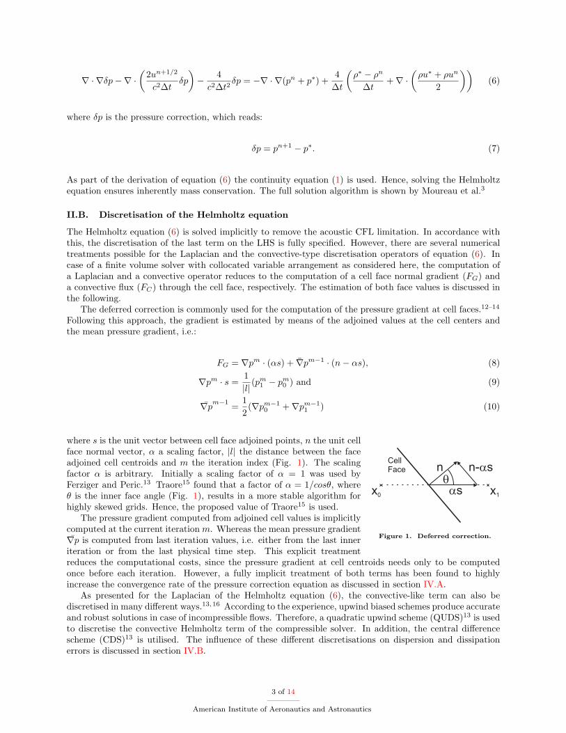
where s is the unit vector between cell face adjoined points, n the unit cellface normal vector, � a scaling factor, jlj the distance between the faceadjoined cell centroids and m the iteration index (Fig. 1). The scalingfactor � is arbitrary. Initially a scaling factor of � = 1 was used byFerziger and Peric.13 Traore15 found that a factor of � = 1=cos�, where� is the inner face angle (Fig. 1), results in a more stable algorithm forhighly skewed grids. Hence, the proposed value of Traore15 is used.

The pressure gradient computed from adjoined cell values is implicitlycomputed at the current iteration m. Whereas the mean pressure gradient�rp is computed from last iteration values, i.e. either from the last inner

iteration or from the last physical time step. This explicit treatmentreduces the computational costs, since the pressure gradient at cell centroids needs only to be computedonce before each iteration. However, a fully implicit treatment of both terms has been found to highlyincrease the convergence rate of the pressure correction equation as discussed in section IV.A.

As presented for the Laplacian of the Helmholtz equation (6), the convective-like term can also bediscretised in many di�erent ways.13,16 According to the experience, upwind biased schemes produce accurateand robust solutions in case of incompressible ows. Therefore, a quadratic upwind scheme (QUDS)13 is usedto discretise the convective Helmholtz term of the compressible solver. In addition, the central di�erencescheme (CDS)13 is utilised. The in uence of these di�erent discretisations on dispersion and dissipationerrors is discussed in section IV.B.

3 of 14

American Institute of Aeronautics and Astronautics

III. Characteristic Boundary Conditions

The computational domain of a CFD simulation usually only comprises a part of the physical domain dueto limitations of computational resources and turn around times.17 Therefore, arti�cial boundaries have

to be introduced. In case of a hyperbolic systems, such as the Helmholtz equation discussed here, arti�cialboundaries are usually derived from the analysis of di�erent waves crossing the boundary.18 The classicalapproach for this are the Navier-Stockes Characteristics Boundary Conditions (NSCBC).19 Generally speak-ing, characteristic equations are solved at boundaries allowing for a separate treatment of boundary crossingwaves.

The classical NSCBC method involves a explicit integration of the characteristic equations, which resultsin a CFL limitation at the boundary adjoined cells.3 To remove this CFL limitation at boundaries, thecharacteristic equations are solved implicitly by means of Dirichlet boundary conditions. In the followingthis method is shown.

III.A. Characteristic Helmholtz Equation

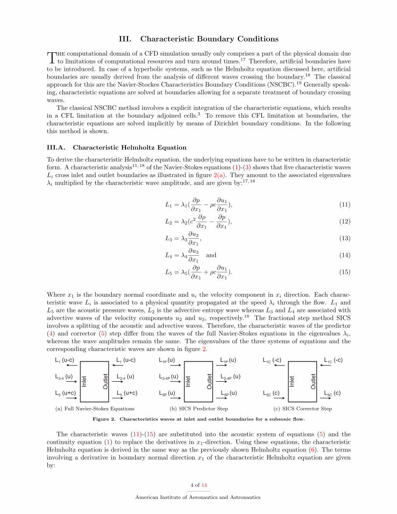
To derive the characteristic Helmholtz equation, the underlying equations have to be written in characteristicform. A characteristic analysis11,18 of the Navier-Stokes equations (1)-(3) shows that �ve characteristic wavesLi cross inlet and outlet boundaries as illustrated in �gure 2(a). They amount to the associated eigenvalues�i multiplied by the characteristic wave amplitude, and are given by:17,18

L1 = �1(@p

@x1� �c@u1

@x1); (11)

L2 = �2(c2@�

@x1� @p

@x1); (12)

L3 = �3@u2

@x1; (13)

L4 = �4@u3

@x1and (14)

L5 = �5(@p

@x1+ �c

@u1

@x1): (15)

Where x1 is the boundary normal coordinate and ui the velocity component in xi direction. Each charac-teristic wave Li is associated to a physical quantity propagated at the speed �i through the ow. L1 andL5 are the acoustic pressure waves, L2 is the advective entropy wave whereas L3 and L4 are associated withadvective waves of the velocity components u2 and u3, respectively.18 The fractional step method SICSinvolves a splitting of the acoustic and advective waves. Therefore, the characteristic waves of the predictor(4) and corrector (5) step di�er from the waves of the full Navier-Stokes equations in the eigenvalues �i,whereas the wave amplitudes remain the same. The eigenvalues of the three systems of equations and thecorresponding characteristic waves are shown in �gure 2.

L (u-c)1

L (u)2-4

L (u+c)5

L (u-c)1

L (u)2-4

L (u+c)5

Inle

t

Ou

tle

t

(a) Full Navier-Stokes Equations

L (u)1P

L (u)2-4P

L (u)5P

L (u)1P

L (u)2-4P

L (u)5P

Inle

t

Ou

tle

t

(b) SICS Predictor Step

L (-c)1C

L (c)5C

L (-c)1C

L (c)5C

Inle

t

Ou

tle

t

(c) SICS Corrector Step

Figure 2. Characteristics waves at inlet and outlet boundaries for a subsonic ow.

The characteristic waves (11)-(15) are substituted into the acoustic system of equations (5) and thecontinuity equation (1) to replace the derivatives in x1-direction. Using these equations, the characteristicHelmholtz equation is derived in the same way as the previously shown Helmholtz equation (6). The termsinvolving a derivative in boundary normal direction x1 of the characteristic Helmholtz equation are givenby:

4 of 14

American Institute of Aeronautics and Astronautics

@2�p

@x21

=@

@x1

�L�5C � L�1C

2c

�; (16)

@un+1�p

@x1= u

n+1=21

�L�5C + L�1C

2c

�+ �p

Ln+1=25C � Ln+1=2

1C

2�c

!; (17)

@2pn

@x21

=@

@x1

�Ln5C � Ln1C

2c

�; (18)

@2p�

@x21

=@

@x1

�L�5C � L�1C

2c

�; (19)

@�u�

@x1=L�5C + L�1C

2c2and (20)

@�un

@x1=

1c2

�Ln2 +

12

(Ln5 + Ln1 )�

(21)

where the time level �, e.g. L�i , is computed as di�erence between the waves at new and advected time level:

L�i = Ln+1i � L�i : (22)

Substituting equations (16)-(21) into (6) gives the characteristic Helmholtz equation, which is solved atboundaries according to the NSCBC method.

The key advantage of the characteristic equation is the ability to compute the characteristic wavescrossing a boundary separately. Following characteristics theory,20 outgoing waves are computed from innerpoints since information propagates out of the computational domain. Incoming waves are either computedfrom known information about the outside of a domain or they have to be approximated.18 Among others,incoming waves are sent in to avoid a drift in mean ow values, e.g. to apply the far �eld pressure at anoutlet boundary. In this scope, Poinsot and Lelle19 proposed to set the incoming wave amplitude to

Lin = K(p� p1) with (23)

K = �c(1�Ma2)=L: (24)

WhereK is a relaxation coe�cient, p the predicted pressure, p1 the far �eld pressure, � a coupling parameter,c the speed of sound, Ma a reference Mach number and L a reference length. Applying the incoming wave(23) reduces the drift of mean values with increasing relaxation coe�cient of the boundary condition, i.e.with increasing K. However, increasing the relaxation coe�cient also increases the re ection at the boundary.The magnitude of the analytical re ection factor reads:21

jjRjj = 1q1 +

�2!K

�2 (25)

where R is the re ection factor and ! the angular frequency. This analytical expression of the re ectionfactor is used in section IV.C to asses the accuracy of the implemented boundary conditions.

III.B. Extrapolation Methods

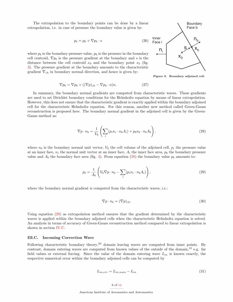
The characteristic Helmholtz equation derived in section III.A is solved implicitly within the boundaryadjoined cells (�g. 3). In this scope, the boundary normal gradients de�ned by equations (16)-(21) areused to extrapolate pressure and velocity values on the boundaries. These values are then used in turn asDirichlet boundary conditions of the characteristic Helmholtz equation.

5 of 14

American Institute of Aeronautics and Astronautics

ni

nb

BoundaryFace b

InnerFace i

xb

x0

s

Figure 3. Boundary adjoined cell.

The extrapolation to the boundary points can be done by a linearextrapolation, i.e. in case of pressure the boundary value is given by:

pb = p0 +rpb � s (26)

where pb is the boundary pressure value, p0 is the pressure in the boundarycell centroid, rpb is the pressure gradient at the boundary and s is thedistance between the cell centroid x0 and the boundary point xb (�g.3). The pressure gradient at the boundary amounts to the characteristicgradient rch in boundary normal direction, and hence is given by:

rpb = rp0 + ((rp)ch �rp0 � n)n: (27)

In summary, the boundary normal gradients are computed from characteristic waves. These gradientsare used to set Dirichlet boundary conditions for the Helmholtz equation by means of linear extrapolation.However, this does not ensure that the characteristic gradient is exactly applied within the boundary adjoinedcell for the characteristic Helmholtz equation. For this reason, another new method called Green-Gaussreconstruction is proposed here. The boundary normal gradient in the adjoined cell is given by the Green-Gauss method as:

rp � nb =1V0

Xi

(pini � nbAi) + pbnb � nbAb

!; (28)

where nb is the boundary normal unit vector, V0 the cell volume of the adjoined cell, pi the pressure valueat an inner face, ni the normal unit vector at an inner face, Ai the inner face area, pb the boundary pressurevalue and Ab the boundary face area (�g. 3). From equation (28) the boundary value pb amounts to:

pb =1Ab

V0rp � nb �

Xi

(pini � nbAi)

!; (29)

where the boundary normal gradient is computed from the characteristic waves, i.e.:

rp � nb = (rp)ch: (30)

Using equation (29) as extrapolation method ensures that the gradient determined by the characteristicwaves is applied within the boundary adjoined cells when the characteristic Helmholtz equation is solved.An analysis in terms of accuracy of Green-Gauss reconstruction method compared to linear extrapolation isshown in section IV.C.

III.C. Incoming Correction Wave

Following characteristic boundary theory,20 domain leaving waves are computed from inner points. Bycontrast, domain entering waves are computed from known values of the outside of the domain,18 e.g. far�eld values or external forcing. Since the value of the domain entering wave Lin is known exactly, therespective numerical error within the boundary adjoined cells can be computed by

Lin;err = Lin;num � Lin (31)

6 of 14

American Institute of Aeronautics and Astronautics

where Lin and Lin;num are the imposed and the numerical incoming waves, respectively. The numericalincoming wave is computed from pressure and velocity gradients within the boundary adjoined cells. Thiserror estimation is used as control variable by applying the correction wave

Lmin;corr = �Lm�1in;err (32)

as additional forcing function. The error is approximated from the last time step or last inner iteration. Thismeasure gives a higher accuracy when imposing external values as discussed in section IV.C.

IV. Results

Within the preceding sections, the fractional step method SICS was introduced, and di�erent measuresused for the implementation of SICS within the DLR THETA code were presented. In the following sub-sections, the impact of these measures is discussed. Finally, results of the Entropy Wave Generator (EWG)test case of Bake et al.10 are shown as validation of the implementation.

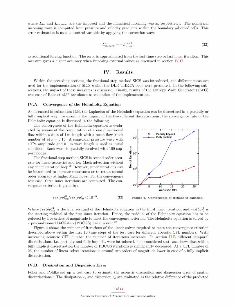
IV.A. Convergence of the Helmholtz Equation

As discussed in subsection II.B, the Laplacian of the Helmholtz equation can be discretised in a partially orfully implicit way. To examine the impact of the two di�erent discretisations, the convergence rate of theHelmholtz equation is discussed in the following.

Acoustic CFL

No

. of

Iter

atio

ns

0 5 10 15 20 25100

101

102

103Partialy ImplicitFully Implicit

Figure 4. Convergence of Helmholtz equation.

The convergence of the Helmholtz equation is evalu-ated by means of the computation of a one dimensional ow within a duct of 1 m length with a mean ow Machnumber of Ma = 0:15. A sinusoidal pressure wave with10 Pa amplitude and 0.1 m wave length is used as initialcondition. Each wave is spatially resolved with 100 sup-port nodes.

The fractional step method SICS is second order accu-rate for linear acoustics and low Mach advection withoutany inner iteration loop.3 However, inner iterations canbe introduced to increase robustness or to retain secondorder accuracy at higher Mach ows. For the convergencetest case, three inner iterations are computed. The con-vergence criterion is given by:

res(�p)3m=res(�p)10 < 10�5: (33)

Where res(�p)3m is the �nal residual of the Helmholtz equation in the third inner iteration, and res(�p)10 isthe starting residual of the �rst inner iteration. Hence, the residual of the Helmholtz equation has to bereduced by �ve orders of magnitude to meet the convergence criterion. The Helmholtz equation is solved bya preconditioned BiCGstab (PBCGS) linear solver.22

Figure 4 shows the number of iterations of the linear solver required to meet the convergence criteriondescribed above within the �rst 10 time steps of the test case for di�erent acoustic CFL numbers. Withincreasing acoustic CFL number the number of iterations increases. In section II.B di�erent temporaldiscretisations, i.e. partially and fully implicit, were introduced. The considered test case shows that with afully implicit discretisation the number of PBCGS iterations is signi�cantly decreased. At a CFL number of25, the number of linear solver iterations is around two orders of magnitude lower in case of a fully implicitdiscretisation.

IV.B. Dissipation and Dispersion Error

F�oller and Polifke set up a test case to estimate the acoustic dissipation and dispersion error of spatialdiscretisations.9 The dissipation �p̂ and dispersion �� are evaluated as the relative di�erence of the predicted

7 of 14

American Institute of Aeronautics and Astronautics

and exact pressure amplitude and wave length, respectively, i.e.:

�p̂ =p̂� p̂num

p̂and (34)

�� =�� �num

�: (35)

Where p̂, p̂num, � and �num are the exact pressure amplitude, the predicted amplitude, the exact wavelength and the predicted wave length, respectively. The dissipation and dispersion errors are measuredafter a 100 Hz sine wave with amplitude of 0.2 m/s was propagated a distance of 10 wave lengths in a one-dimensional duct with mean ow velocity of 0.25 m/s. The sine waves are spatially resolved by 10 to 40points per wave length (PPW).

F�oller and Polifke computed the error of the second order Lax-Wendro� (LW) scheme implementedinto the AVPB23 solver.9 Moreover, Gunasekaran and McGuirk used the test case to asses the error ofthe second order Total Variation Diminishing (TVD) and �fth order weighted essentially non-oscillatory(WENO) schemes.4 As part of this discussion, the acoustic error is computed for the second order schemesQUDS and CDS implemented in DLR THETA code (sec. II.B).

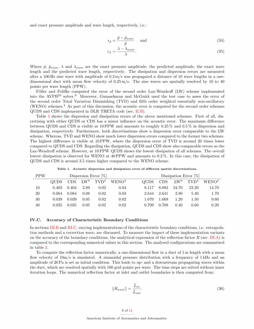
Table 1 shows the dispersion and dissipation errors of the above mentioned schemes. First of all, dis-cretising with either QUDS or CDS has a minor in uence on the acoustic error. The maximum di�erencebetween QUDS and CDS is visible at 10 PPW and amounts to roughly 0.25 % and 0.5 % in dispersion anddissipation, respectively. Furthermore, both discretisations show a dispersion error comparable to the LWscheme. Whereas, TVD and WENO show much lower dispersion errors compared to the former two schemes.The highest di�erence is visible at 10 PPW, where the dispersion error of TVD is around 20 times lowercompared to QUDS and CDS. Regarding the dissipation, QUDS and CDS show also comparable errors as theLax-Wendro� scheme. However, at 10 PPW QUDS shows the lowest dissipation of all schemes. The overalllowest dissipation is observed for WENO at 40 PPW and amounts to 0.2 %. In this case, the dissipation ofQUDS and CDS is around 3.5 times higher compared to the WENO scheme.

Table 1. Acoustic dispersion and dissipation error of di�erent spatial discretisations.

PPW Dispersion Error [%] Dissipation Error [%]QUDS CDS LW9 TVD4 WENO4 QUDS CDS LW9 TVD4 WENO4

10 0.403 0.404 2.89 0.02 0.04 8.117 8.082 34.70 23.20 14.7020 0.084 0.084 0.08 0.02 0.03 2.644 2.641 2.80 5.40 1.7030 0.039 0.039 0.05 0.02 0.02 1.670 1.669 1.20 1.50 0.6040 0.035 0.035 0.05 0.02 0.02 0.709 0.708 0.40 0.60 0.20

IV.C. Accuracy of Characteristic Boundary Conditions

In sections III.B and III.C, varying implementations of the characteristic boundary conditions, i.e. extrapola-tion methods and a correction wave, are discussed. To measure the impact of these implementation variantson the accuracy of the boundary conditions, the analytical expression of the re ection factor R (sec. III.A) iscompared to the corresponding numerical values in this section. The analysed con�gurations are summarisedin table 2.

To compute the re ection factor numerically, a one-dimensional ow in a duct of 1 m length with a mean ow velocity of 10m/s is simulated. A sinusoidal pressure distribution with a frequency of 1 kHz and anamplitude of 20 Pa is set as initial condition. This leads to up- and a downstream propagating waves withinthe duct, which are resolved spatially with 100 grid points per wave. The time steps are solved without inneriteration loops. The numerical re ection factor at inlet and outlet boundaries is then computed from:

jjRnumjj =L̂in

L̂out: (36)

8 of 14

American Institute of Aeronautics and Astronautics

where L̂in and L̂out are the amplitudes of incoming and outgoing acoustic waves, respectively. At both,the inlet and outlet boundaries, the relaxation coe�cient K is varied instead of the frequency of the initialpressure waves. This is a more convenient approach.21 The value of K is varied between 102 and 105. Thelower limit of K corresponds roughly to a coupling parameter of � = 0:27 which is the theoretically derivedoptimum.24 Whereas, a K value of 2 � 102 is equal to the best practise value of � = 0:58.18,19 The upperlimit of the considered K values results in an almost fully re ective boundary condition.

Table 2. Con�gurations analysed in view of boundary re ection.

Con�guration Extrapolation method Correction WaveBaseline Green-Gauss onw/o Correction Wave Green-Gauss o�Linear Extrapolation Linear on

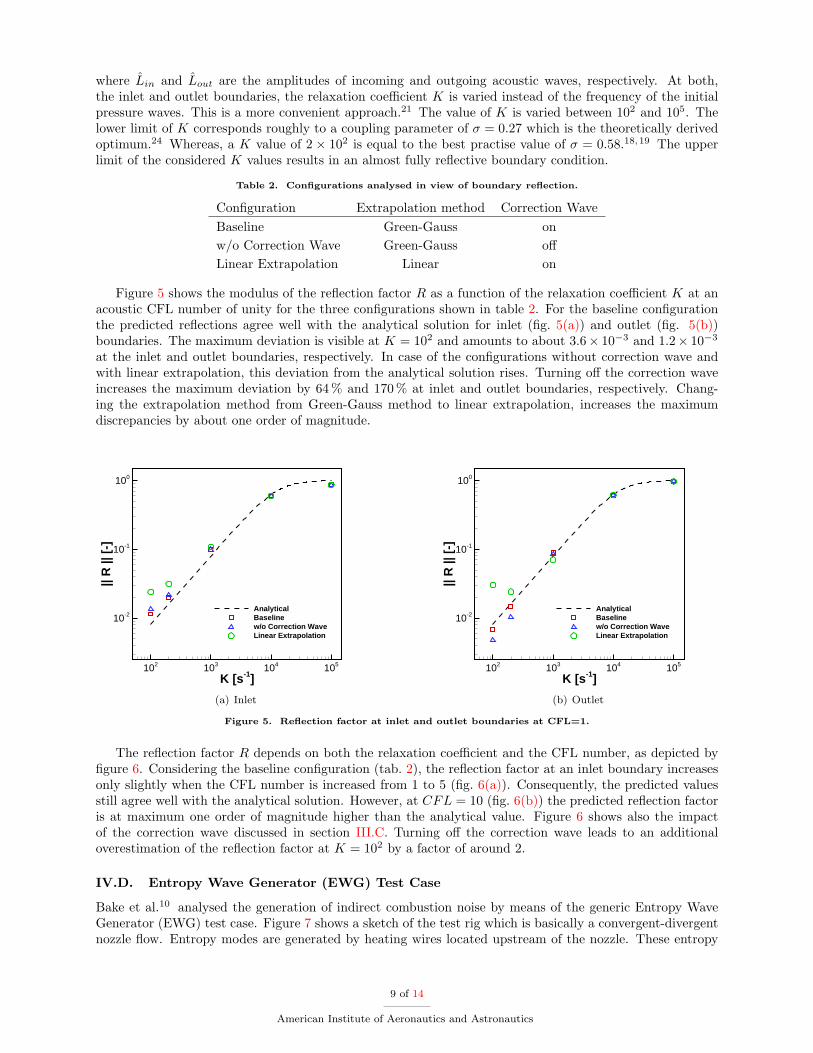
Figure 5 shows the modulus of the re ection factor R as a function of the relaxation coe�cient K at anacoustic CFL number of unity for the three con�gurations shown in table 2. For the baseline con�gurationthe predicted re ections agree well with the analytical solution for inlet (�g. 5(a)) and outlet (�g. 5(b))boundaries. The maximum deviation is visible at K = 102 and amounts to about 3:6� 10�3 and 1:2� 10�3

at the inlet and outlet boundaries, respectively. In case of the con�gurations without correction wave andwith linear extrapolation, this deviation from the analytical solution rises. Turning o� the correction waveincreases the maximum deviation by 64 % and 170 % at inlet and outlet boundaries, respectively. Chang-ing the extrapolation method from Green-Gauss method to linear extrapolation, increases the maximumdiscrepancies by about one order of magnitude.

K [s-1]

|| R

|| [

-]

102 103 104 105

10-2

10-1

100

AnalyticalBaselinew/o Correction WaveLinear Extrapolation

(a) Inlet

K [s-1]

|| R

|| [

-]

102 103 104 105

10-2

10-1

100

AnalyticalBaselinew/o Correction WaveLinear Extrapolation

(b) Outlet

Figure 5. Re ection factor at inlet and outlet boundaries at CFL=1.

The re ection factor R depends on both the relaxation coe�cient and the CFL number, as depicted by�gure 6. Considering the baseline con�guration (tab. 2), the re ection factor at an inlet boundary increasesonly slightly when the CFL number is increased from 1 to 5 (�g. 6(a)). Consequently, the predicted valuesstill agree well with the analytical solution. However, at CFL = 10 (�g. 6(b)) the predicted re ection factoris at maximum one order of magnitude higher than the analytical value. Figure 6 shows also the impactof the correction wave discussed in section III.C. Turning o� the correction wave leads to an additionaloverestimation of the re ection factor at K = 102 by a factor of around 2.

IV.D. Entropy Wave Generator (EWG) Test Case

Bake et al.10 analysed the generation of indirect combustion noise by means of the generic Entropy WaveGenerator (EWG) test case. Figure 7 shows a sketch of the test rig which is basically a convergent-divergentnozzle ow. Entropy modes are generated by heating wires located upstream of the nozzle. These entropy

9 of 14

American Institute of Aeronautics and Astronautics

K [s-1]

|| R

|| [

-]

102 103 104 105

10-2

10-1

100

AnalyticalBaseline, CFL=1Baseline, CFL=5w/o Correction, CFL=5

(a) CFL=5

K [s-1]

|| R

|| [

-]

102 103 104 105

10-2

10-1

100

AnalyticalBaseline, CFL=1Baseline, CFL=10w/o Correction, CFL=10

(b) CFL=10

Figure 6. Re ection factor at the inlet boundary for di�erent CFL numbers.

modes are convected and accelerated through the nozzle, which gives rise to pressure uctuations downstreamof the nozzle.

Figure 7. Sketch of the Entropy Wave Generator test rig.10

Table 3 summarises the geometrical dimensions of the analysed test case. All axial positions are measuredfrom the most downstream heating wire. Further details are given by Bake et al.10 and M�uhlbauer et al.25

The heating power is adjusted to give a temperature increase of around �T � 9 K. Temperature uctuationsare measured by means of a bare wire thermocouple located between the heating module and the nozzle.Moreover, pressure uctuations are gained at four positions downstream of the nozzle (tab. 3).

Table 3. Dimensions of EWG test case.10

Device Axial Position [mm] Diameter [mm]Thermocouple 34Nozzle 105.5 7.5Microphone 1 456Microphone 2 836Microphone 3 1081Microphone 4 1256

For this discussion, numerical simulations with the DLR THETA code are carried out for di�erent mass ow rates between 6 and 30 kg=h. Due to the rotational symmetry of the test rig, only a 10� slice of the owis simulated. This slice is discretised by around 125 k grid points. The momentum and turbulence transportequations are spatially discretised by means of a second order quadratic upwind scheme (QUDS), whereas

10 of 14

American Institute of Aeronautics and Astronautics

all remaining equations are disctretised centrally (CDS). Turbulent uctuations are modeled by means ofk � ! SST turbulence model.26 Acoustic perturbations at frequencies lower than 3 kHz are resolved with atleast 50 PPW, which gives very low dispersion and dissipation errors (sec. IV.B). As shown by Bake et al.,10

the acoustic impedance of the downstream termination of the exible tube section of the test rig (�g. 7) canbe modeled by means of characteristic boundary conditions. Applying a coupling parameter of � = 1:8 atthe downstream termination reproduces the experimentally measured pressure uctuations accurately.10,25

Therefore, this value of the coupling parameter is also used for the computations presented in this discussion.Furthermore, data computed with ANSYS CFX 11.0 are used as validation of the THETA results. Thesedata are provided by B. M�uhlbauer and it was shown that they agree very well with the measurements ofBake et al.10 The corresponding numerical setup is described in detail by M�uhlbauer et al.25

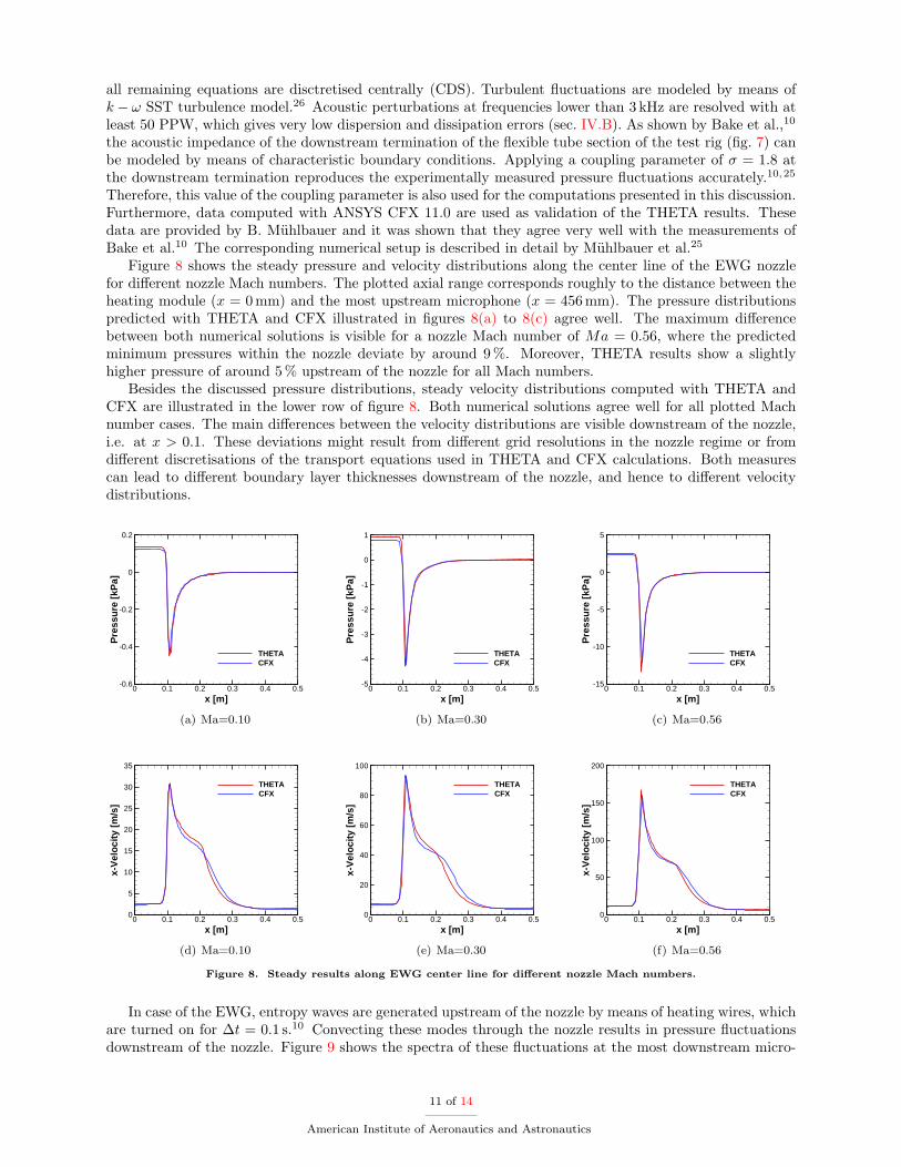
Figure 8 shows the steady pressure and velocity distributions along the center line of the EWG nozzlefor di�erent nozzle Mach numbers. The plotted axial range corresponds roughly to the distance between theheating module (x = 0 mm) and the most upstream microphone (x = 456 mm). The pressure distributionspredicted with THETA and CFX illustrated in �gures 8(a) to 8(c) agree well. The maximum di�erencebetween both numerical solutions is visible for a nozzle Mach number of Ma = 0:56, where the predictedminimum pressures within the nozzle deviate by around 9 %. Moreover, THETA results show a slightlyhigher pressure of around 5 % upstream of the nozzle for all Mach numbers.

Besides the discussed pressure distributions, steady velocity distributions computed with THETA andCFX are illustrated in the lower row of �gure 8. Both numerical solutions agree well for all plotted Machnumber cases. The main di�erences between the velocity distributions are visible downstream of the nozzle,i.e. at x > 0:1. These deviations might result from di�erent grid resolutions in the nozzle regime or fromdi�erent discretisations of the transport equations used in THETA and CFX calculations. Both measurescan lead to di�erent boundary layer thicknesses downstream of the nozzle, and hence to di�erent velocitydistributions.

x [m]

Pre

ssu

re [

kPa]

0 0.1 0.2 0.3 0.4 0.5-0.6

-0.4

-0.2

0

0.2

THETACFX

(a) Ma=0.10

x [m]

Pre

ssu

re [

kPa]

0 0.1 0.2 0.3 0.4 0.5-5

-4

-3

-2

-1

0

1

THETACFX

(b) Ma=0.30

x [m]

Pre

ssu

re [

kPa]

0 0.1 0.2 0.3 0.4 0.5-15

-10

-5

0

5

THETACFX

(c) Ma=0.56

x [m]

x-V

elo

city

[m

/s]

0 0.1 0.2 0.3 0.4 0.50

5

10

15

20

25

30

35

THETACFX

(d) Ma=0.10

x [m]

x-V

elo

city

[m

/s]

0 0.1 0.2 0.3 0.4 0.50

20

40

60

80

100

THETACFX

(e) Ma=0.30

x [m]

x-V

elo

city

[m

/s]

0 0.1 0.2 0.3 0.4 0.50

50

100

150

200

THETACFX

(f) Ma=0.56

Figure 8. Steady results along EWG center line for di�erent nozzle Mach numbers.

In case of the EWG, entropy waves are generated upstream of the nozzle by means of heating wires, whichare turned on for �t = 0:1 s.10 Convecting these modes through the nozzle results in pressure uctuationsdownstream of the nozzle. Figure 9 shows the spectra of these uctuations at the most downstream micro-

11 of 14

American Institute of Aeronautics and Astronautics

f [Hz]

SP

L [

dB

]

0 50 100 150 2000

20

40

60

80

100

THETACFX

(a) Ma=0.10

f [Hz]

SP

L [

dB

]

0 50 100 150 2000

20

40

60

80

100

THETACFX

(b) Ma=0.30

f [Hz]

SP

L [

dB

]

0 50 100 150 2000

20

40

60

80

100

THETACFX

(c) Ma=0.56

Figure 9. Spectra of the predicted pressure signals for di�erent nozzle Mach numbers.

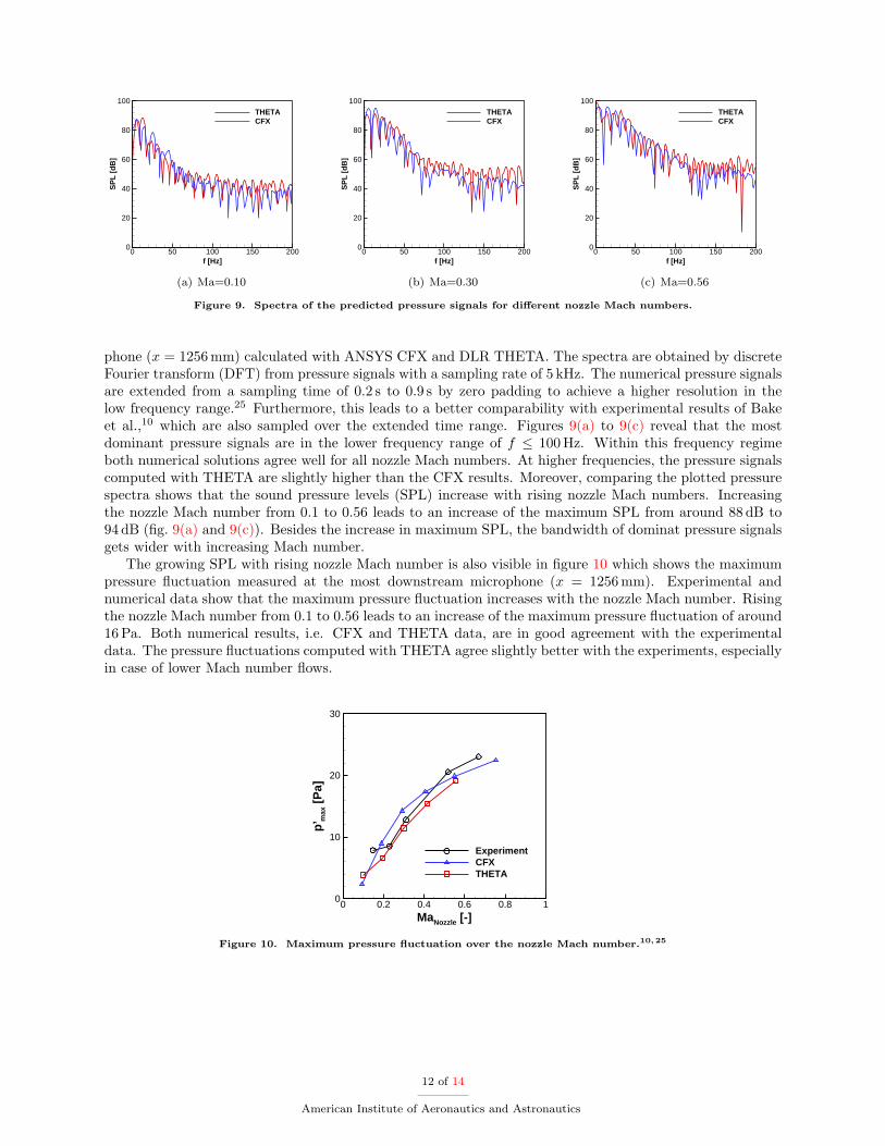
phone (x = 1256 mm) calculated with ANSYS CFX and DLR THETA. The spectra are obtained by discreteFourier transform (DFT) from pressure signals with a sampling rate of 5 kHz. The numerical pressure signalsare extended from a sampling time of 0.2 s to 0.9 s by zero padding to achieve a higher resolution in thelow frequency range.25 Furthermore, this leads to a better comparability with experimental results of Bakeet al.,10 which are also sampled over the extended time range. Figures 9(a) to 9(c) reveal that the mostdominant pressure signals are in the lower frequency range of f � 100 Hz. Within this frequency regimeboth numerical solutions agree well for all nozzle Mach numbers. At higher frequencies, the pressure signalscomputed with THETA are slightly higher than the CFX results. Moreover, comparing the plotted pressurespectra shows that the sound pressure levels (SPL) increase with rising nozzle Mach numbers. Increasingthe nozzle Mach number from 0:1 to 0:56 leads to an increase of the maximum SPL from around 88 dB to94 dB (�g. 9(a) and 9(c)). Besides the increase in maximum SPL, the bandwidth of dominat pressure signalsgets wider with increasing Mach number.

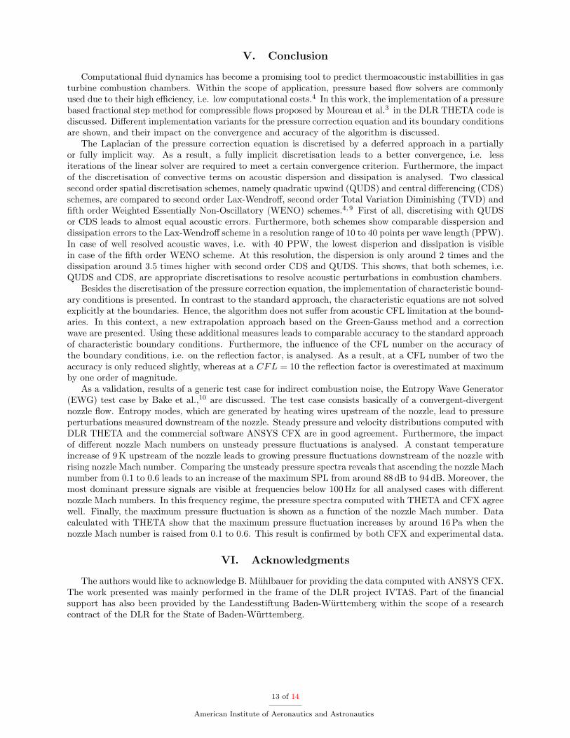
The growing SPL with rising nozzle Mach number is also visible in �gure 10 which shows the maximumpressure uctuation measured at the most downstream microphone (x = 1256 mm). Experimental andnumerical data show that the maximum pressure uctuation increases with the nozzle Mach number. Risingthe nozzle Mach number from 0.1 to 0.56 leads to an increase of the maximum pressure uctuation of around16 Pa. Both numerical results, i.e. CFX and THETA data, are in good agreement with the experimentaldata. The pressure uctuations computed with THETA agree slightly better with the experiments, especiallyin case of lower Mach number ows.

MaNozzle [-]

p’ m

ax [

Pa]

0 0.2 0.4 0.6 0.8 10

10

20

30

ExperimentCFXTHETA

Figure 10. Maximum pressure uctuation over the nozzle Mach number.10,25

12 of 14

American Institute of Aeronautics and Astronautics

V. Conclusion

Computational uid dynamics has become a promising tool to predict thermoacoustic instabillities in gasturbine combustion chambers. Within the scope of application, pressure based ow solvers are commonlyused due to their high e�ciency, i.e. low computational costs.4 In this work, the implementation of a pressurebased fractional step method for compressible ows proposed by Moureau et al.3 in the DLR THETA code isdiscussed. Di�erent implementation variants for the pressure correction equation and its boundary conditionsare shown, and their impact on the convergence and accuracy of the algorithm is discussed.

The Laplacian of the pressure correction equation is discretised by a deferred approach in a partiallyor fully implicit way. As a result, a fully implicit discretisation leads to a better convergence, i.e. lessiterations of the linear solver are required to meet a certain convergence criterion. Furthermore, the impactof the discretisation of convective terms on acoustic dispersion and dissipation is analysed. Two classicalsecond order spatial discretisation schemes, namely quadratic upwind (QUDS) and central di�erencing (CDS)schemes, are compared to second order Lax-Wendro�, second order Total Variation Diminishing (TVD) and�fth order Weighted Essentially Non-Oscillatory (WENO) schemes.4,9 First of all, discretising with QUDSor CDS leads to almost equal acoustic errors. Furthermore, both schemes show comparable disspersion anddissipation errors to the Lax-Wendro� scheme in a resolution range of 10 to 40 points per wave length (PPW).In case of well resolved acoustic waves, i.e. with 40 PPW, the lowest disperion and dissipation is visiblein case of the �fth order WENO scheme. At this resolution, the dispersion is only around 2 times and thedissipation around 3.5 times higher with second order CDS and QUDS. This shows, that both schemes, i.e.QUDS and CDS, are appropriate discretisations to resolve acoustic perturbations in combustion chambers.

Besides the discretisation of the pressure correction equation, the implementation of characteristic bound-ary conditions is presented. In contrast to the standard approach, the characteristic equations are not solvedexplicitly at the boundaries. Hence, the algorithm does not su�er from acoustic CFL limitation at the bound-aries. In this context, a new extrapolation approach based on the Green-Gauss method and a correctionwave are presented. Using these additional measures leads to comparable accuracy to the standard approachof characteristic boundary conditions. Furthermore, the in uence of the CFL number on the accuracy ofthe boundary conditions, i.e. on the re ection factor, is analysed. As a result, at a CFL number of two theaccuracy is only reduced slightly, whereas at a CFL = 10 the re ection factor is overestimated at maximumby one order of magnitude.

As a validation, results of a generic test case for indirect combustion noise, the Entropy Wave Generator(EWG) test case by Bake et al.,10 are discussed. The test case consists basically of a convergent-divergentnozzle ow. Entropy modes, which are generated by heating wires upstream of the nozzle, lead to pressureperturbations measured downstream of the nozzle. Steady pressure and velocity distributions computed withDLR THETA and the commercial software ANSYS CFX are in good agreement. Furthermore, the impactof di�erent nozzle Mach numbers on unsteady pressure uctuations is analysed. A constant temperatureincrease of 9 K upstream of the nozzle leads to growing pressure uctuations downstream of the nozzle withrising nozzle Mach number. Comparing the unsteady pressure spectra reveals that ascending the nozzle Machnumber from 0.1 to 0.6 leads to an increase of the maximum SPL from around 88 dB to 94 dB. Moreover, themost dominant pressure signals are visible at frequencies below 100 Hz for all analysed cases with di�erentnozzle Mach numbers. In this frequency regime, the pressure spectra computed with THETA and CFX agreewell. Finally, the maximum pressure uctuation is shown as a function of the nozzle Mach number. Datacalculated with THETA show that the maximum pressure uctuation increases by around 16 Pa when thenozzle Mach number is raised from 0.1 to 0.6. This result is con�rmed by both CFX and experimental data.

VI. Acknowledgments

The authors would like to acknowledge B. M�uhlbauer for providing the data computed with ANSYS CFX.The work presented was mainly performed in the frame of the DLR project IVTAS. Part of the �nancialsupport has also been provided by the Landesstiftung Baden-W�urttemberg within the scope of a researchcontract of the DLR for the State of Baden-W�urttemberg.

13 of 14

American Institute of Aeronautics and Astronautics

References

1Moeck, J., Bothien, M., Schimek, S., Lacarelle, A., and Paschereit, C., \Subcritical thermoacoustic instabilites in apremixed combustor," AIAA Paper 2008-2946 , 2008.

2Lieuwen, T. and Yang, V., Combustion instabilities in gas turbine engines: operational experience, fundamental mecha-nisms and modeling, AIAA Inc., 2005.

3Moureau, V., B�erat, C., and Pitsch, H., \An e�cient semi-implicit compressible solver for large-eddy simulations," J.Comput. Phys., Vol. 226, No. 2, 2007, pp. 1256{1270.

4Gunasekaran, B. and McGuirk, J. J., \Mildly-compressible pressure-based CFD methodology for acoustic propagationand absorption prediction," Proceedings of ASME Turbo Expo 2011 , 2011.

5Chorin, A., \Numerical solution of the Navier-Stokes equations," Mathematics of Computation, Vol. 22, No. 104, 1968,pp. 745{762.

6Kim, J. and Moin, P., \Application of a fractional-step method to incompressible Navier-Stokes equations," Journal ofComputational Physics, Vol. 59, No. 2, 1985, pp. 308{323.

7Pierce, C., Progress-Variable Approach for Large-Eddy Simulation of Turbulent Combustion, Ph.D. thesis, StanfordUniversity, 2001.

8Di Domenico, M., Numerical Simulation of Soot Formation in Turbulent Flows, Ph.d. thesis, University of Stuttgart,2008.

9F�oller, S. and Polifke, W., \Determination of Acoustic Transfer Matrices via Large Eddy Simulation and System Identi-�cation," 16th AIAA/CEAS Aeroacoustics Conference.4

10Bake, F., Richter, C., M�uhlbauer, B., Kings, N., R�ohle, I., Thiele, F., and Noll, B., \The Entropy Wave Generator(EWG): A reference case on entropy noise," Journal of Sound and Vibration, 2009.

11Thompson, K., \Time Dependent Boundary Conditions for Hyperbolic Systems," Journal of Computational Physics,Vol. 68, 1986, pp. 1{24.

12Khosla, P. and Rubin, S., \A diagonally dominant second-order accurate implicit scheme," Computers and Fluids, Vol. 2,No. 2, 1974, pp. 207 { 209.

13Ferziger, J. and Peric, M., Computational Methods for Fluid Dynamics, 2002.14Zwart, P., Raithby, G., and Raw, M., \An integrated space-time �nite-volume method for moving-boundary problems,"

Numerical Heat Transfer, Part B: Fundamentals, Vol. 34, No. 3, 1998, pp. 257{270.15Traore, P., Ahipo, Y. M., and Louste, C., \A robust and e�cient �nite volume scheme for the discretization of di�usive

ux on extremely skewed meshes in complex geometries," Journal of Computational Physics,14 pp. 5148{5159, pp. 5148{5159.16Blazek, J., Computational uid dynamics: principles and applications, Vol. 1, Elsevier, 2005.17Widenhorn, A., Noll, B., and Aigner, M., \Accurate Boundary Conditions for the Numerical Simulation of Thermoacoustic

Phenomena in Gas-Turbine Combustion Chambers," ASME Turbo Expo 2006 , 2006, pp. 1{10.18Poinsot, T. and Veynante, D., Theoretical and numerical combustion, RT Edwards, Inc., 2005.19Poinsot, T. and Lele, S., \Boundary Conditions for Direct Simulations of Compressible Viscous Flows," Journal of

Computational Physics, Vol. 101, 1992, pp. 104{129.20Kreiss, H.-O., \Boundary conditions for hyperbolic di�erential equations," Conference on the Numerical Solution of

Di�erential Equations, edited by G. Watson, Vol. 363 of Lecture Notes in Mathematics, Springer Berlin / Heidelberg, 1974,pp. 64{74.

21Selle, L., Nicoud, F., and Poinsot, T., \Actual impedance of nonre ecting boundary conditions: implications for compu-tation of resonators," AIAA journal , Vol. 42, No. 5, 2004, pp. 958{964.

22Meister, A., Numerik linearer Gleichungssysteme, Vieweg, Wiesbaden, 3rd ed., 2008.23Schoenfeld, T. and Rudgyardt, M., \Steady and unsteady ow simulations using the hybrid ow solver AVBP," AIAA

journal , Vol. 37, No. 11, 1999, pp. 1378{1385.24Rudy, D. and Strikwerda, J., \A Nonre ecting Out ow Boundary Condition for Subsonic Navier-Stokes Calculations,"

Journal of Computational Physics, Vol. 36, 1980, pp. 55{70.25M�uhlbauer, B., Noll, B., and Aigner, M., \Numerical investigation of the fundamental mechanism for entropy noise

generation in aero-engines," Acta Acustica united with Acustica, Vol. 95, No. 3, 2009, pp. 470{478.26Menter, F., \Two-equation eddy-viscosity turbulence models for engineering applications," AIAA Journal , Vol. 32, No. 8,

1994, pp. 1598{1605.

14 of 14

American Institute of Aeronautics and Astronautics