Dynamic resource allocation for efficient parallel CFD ... - arXiv

Dynamic resource allocation for efficient parallel CFDsimulations

G. Houzeaux, R.M. Badia, R. Borrell, D. Dosimont,J. Ejarque, M. Garcia-Gasulla, V. Lopez

Barcelona Supercomputing Center, Torre Girona,c/ Jordi Girona 31, 08004 Barcelona, Spain

Abstract

CFD users of supercomputers usually resort to rule-of-thumb methods to select thenumber of subdomains (partitions) when relying on MPI-based parallelization. Onecommon approach is to set a minimum number of elements or cells per subdomain,under which the parallel efficiency of the code is ”known” to fall below a subjective level,say 80%. The situation is even worse when the user is not aware of the “good” practicesfor the given code and a huge amount of resources can thus be wasted. This workpresents an elastic computing methodology to adapt at runtime the resources allocatedto a simulation automatically. The criterion to control the required resources is basedon a runtime measure of the communication efficiency of the execution. According tosome analytical estimates, the resources are then expanded or reduced to fulfil thiscriterion and eventually execute an efficient simulation.

1 Introduction

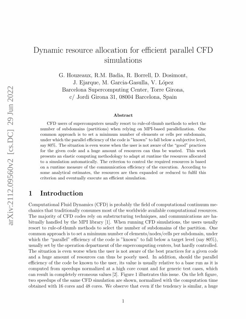
Computational Fluid Dynamics (CFD) is probably the field of computational continuum me-chanics that traditionally consumes most of the worldwide available computational resources.The majority of CFD codes rely on substructuring techniques, and communications are ha-bitually handled by the MPI library [1]. When running CFD simulations, the users usuallyresort to rule-of-thumb methods to select the number of subdomains of the partition. Onecommon approach is to set a minimum number of elements/nodes/cells per subdomain, underwhich the “parallel” efficiency of the code is ”known” to fall below a target level (say 80%),usually set by the operation department of the supercomputing centers, but hardly controlled.The situation is even worse when the user is not aware of the best practices for a given codeand a huge amount of resources can thus be poorly used. In addition, should the parallelefficiency of the code be known to the user, its value is usually relative to a base run as it iscomputed from speedups normalized at a high core count and for generic test cases, whichcan result in completely erroneous values [2]. Figure 1 illustrates this issue. On the left figure,two speedups of the same CFD simulation are shown, normalized with the computation timeobtained with 16 cores and 48 cores. We observe that even if the tendency is similar, a huge

1

arX

iv:2

112.

0956

0v2

[cs

.DC

] 2

9 Ju

n 20

22

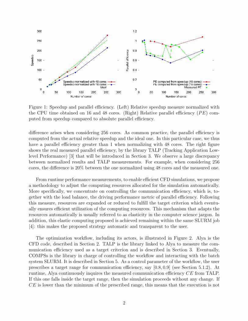
Figure 1: Speedup and parallel efficiency. (Left) Relative speedup measure normalized withthe CPU time obtained on 16 and 48 cores. (Right) Relative parallel efficiency (PE) com-puted from speedup compared to absolute parallel efficiency.

difference arises when considering 256 cores. As common practice, the parallel efficiency iscomputed from the actual relative speedup and the ideal one. In this particular case, we thushave a parallel efficiency greater than 1 when normalizing with 48 cores. The right figureshows the real measured parallel efficiency, by the library TALP (Tracking Application Low-level Performance) [3] that will be introduced in Section 3. We observe a large discrepancybetween normalized results and TALP measurements. For example, when considering 256cores, the difference is 20% between the one normalized using 48 cores and the measured one.

From runtime performance measurements, to enable efficient CFD simulations, we proposea methodology to adjust the computing resources allocated for the simulation automatically.More specifically, we concentrate on controlling the communication efficiency, which is, to-gether with the load balance, the driving performance metric of parallel efficiency. Followingthis measure, resources are expanded or reduced to fulfill the target criterion which eventu-ally ensures efficient utilization of the computing resources. This mechanism that adapts theresources automatically is usually referred to as elasticity in the computer science jargon. Inaddition, this elastic computing proposed is achieved remaining within the same SLURM job[4]: this makes the proposed strategy automatic and transparent to the user.

The optimization workflow, including its actors, is illustrated in Figure 2. Alya is theCFD code, described in Section 2. TALP is the library linked to Alya to measure the com-munication efficiency used as a target criterion and is described in Section 3. Eventually,COMPSs is the library in charge of controlling the workflow and interacting with the batchsystem SLURM. It is described in Section 5. As a control parameter of the workflow, the userprescribes a target range for communication efficiency, say [0.8, 0.9] (see Section 5.1.2). Atruntime, Alya continuously inquires the measured communication efficiency CE from TALP.If this one falls inside the target range, then the simulation proceeds without any change. IfCE is lower than the minimum of the prescribed range, this means that the execution is not

2

Figure 2: Optimizing the resources. Workflow for elastic computing of CFD simulations, in-volving different codes and libraries: Alya (CFD), TALP (efficiency measures) and COMPSs(elastic computing).

efficient enough and resources should be decreased. Employing a simple model, explained inSection 5.1.3, Alya then estimates the number of cores needed to recover the target range.On the contrary, if the measured CE is above the range maximum, resources can be ex-tended, similarly, they are removed. Once the new amount of resources is available, Alyawrites restart files on disk, it is relaunched with a new partitioning, reads the restart files,and resumes the simulation. To ensure restart files can be written and read disregarding thenumber of subdomains, a specific I/O strategy is explained in Section 2.1.1.

Efficiency. This paper presents an autonomous elastic computing methodology to achieveefficient CFD simulations, based on obtaining parallel efficiency metrics at runtime that allowus to estimate the optimum number of computing resources to use. This approach intendsto trade-off power consumption, through controlling the resources to reach a target parallelefficiency, and performance. It thus belongs to the family of energy-to-solution techniques,as opposed to time-to-solution techniques. Traditionally, energy-to-solution techniques havebeen based on hardware parameter tuning, like CPU core frequency, CPU uncore frequency(e.g. cache, memory controller), or the number of OpenMP threads [5, 6, 7, 8]. Applica-tion parameters tuning has also been investigated for example in [9, 10] in the context of theREADEX European project. Our strategy is a resource tuning strategy for MPI applications.

Generic performance analysis. Parallel efficiency, as well as software or hardware coun-ters in general can be obtained with libraries. Tracing tools like Extrae [11], ScoreP [12] or

3

HPCToolkit [13], collect information such as PAPI counters, MPI, and OpenMP calls thathappen during the execution and store them in a trace together with timing information.These traces can then be visualized and analyzed post-mortem with visualization tools avail-able within the library or by specific tools like Paraver [14] or Scalasca [15]. The trace-basedtools provide detailed information on the execution after the application has finished and usu-ally a performance analyst is required to process the data. LIKWID [16] is a command-lineperformance tool suite, which, among other functionalities, provides hardware performancecounters. The different metrics collected can be displayed at runtime with one of the utilitiesprovided in the suite. However, these metrics do not include any parallel efficiency infor-mation, and the user needs to interpret them. Also, the lightweight mpiP library deliversspecific statistical information on MPI calls [17] upon finalization of the execution. In thiswork, we rely on the library TALP, which provides parallel efficiency metrics at runtime. Themetrics collected by TALP are defined in the PoP performance model [18], developed by theresearchers of the European Centre of Excellence Performance Optimisation and Productivity[19]; the PoP metrics are a set of efficiency and scalability indicators that can be obtainedfor MPI applications. In our case, the efficiency metrics reported by TALP allow the user toobtain the parallel efficiency, which is split into communication efficiency and load balance.This allows to compute the optimum number of the computational resources that must beused in the execution to achieve a given parallel efficiency defined by the user.

Performance analysis of CFD codes. As aforementioned, the calculation of the parallelefficiency of simulation codes usually relies on post-mortem analysis. In [20], post-mortemanalyses are performed on three different CFD codes using several performance tools. ThePoP center of excellence [19] offers continuous performance analysis of simulation codes; seefor example [21] for OpenFoam or [22] for AVBP. It is common practice for High-PerformanceComputing (HPC) users to extrapolate parallel efficiency from computed speedup. To thisaim, the speedup is obtained by timing executions of the code on a different number of coresand computing it based on timings for the lowest number of cores. Finally, this parallelefficiency is calculated using the ratio between the measured speedup and the ideal speedup(perfect speedup meaning efficiency of one) [2, 23]. Consequently, these measures are relativeand not absolute. Moreover, they provide information on the timing but not on the paral-lel efficiency achieved. On the contrary, the TALP library considered in this work providesruntime measures of the different metrics composing the real and absolute parallel efficiencyachieved in an execution.

Elasticity. Once the CFD code is adequately instrumented for runtime measures, dynamicresources allocation can be put in place to provide elasticity to the execution. The elasticityterm has become very popular with the evolution of Cloud Computing [24]. Cloud providersand software vendors have developed services to allow users to define rules to automaticallyscale up/down resources of their services when a certain metric reaches a threshold or a cer-tain event is triggered [25]. These auto-scaling services aim at automatically adjusting therequired resources to the application load, and maximize the benefit of the cloud pay-per-usemodel. For HPC systems, where the infrastructure is static but its workloads are dynamic,the elasticity concept has focused on supporting malleable jobs, i.e. applications that sup-port changing the computing resources at runtime. The research on this area has focused

4

on three aspects: i) enabling malleability of jobs using resource managers such as SLURM[26, 4] and OAR [27]; ii) scheduling of malleable jobs [28, 29] and iii) the communicationbetween the application and resource managers [30, 31]. The present work thus proposes anoriginal application of elastic computing to optimize a CFD execution in terms of parallelefficiency.

In the following four sections, we introduce the different components of the workflow,namely Alya, TALP, and COMPSs. We then describe the complete workflow in Section 5.Finally, the proposed strategy is validated by applying the proposed strategy to a series ofCFD simulations in Section 6.

2 CFD code: Alya

2.1 Physical and Numerical Modeling

We consider in this paper the incompressible Navier-Stokes equations as a use case, but thestrategy is extensible to any set of partial differential equations (PDE). We will assess twonumerical schemes based on the finite element method, in which stabilizations depend on thestate of the flow under consideration. For laminar to slightly turbulent flows, we rely on aVariational MultiScale Method (VMS) [32] to stabilize both convection and pressure. Theresulting system is then solved by extracting the pressure Schur complement and eventuallyconverges to the monolithic solution [33]. When considering fully turbulent flows, we ratheropt for a fractional step scheme with a low dissipation scheme (EMAC scheme for convection[34]) and Large Eddy Simulation (LES) turbulence modeling [35]. The main characteristicsof both strategies are summarized in Table 1. The objective of considering these two dis-

Implicit scheme Explicit schemeApplication range Laminar-slightly turbulent Fully turbulentSolution strategy Pressure Schur complement [33] Fractional step [36]Time integration Second order BDF 4th order Runge-Kutta [37]Turbulent modeling ILES Vreman [38]Wall treatment No-slip Law of the wall [39]Convection stab. VMS [32] None [35]Pressure stab. VMS [32] Continuous-discrete LaplacianMomentum solver GMRES ExplicitPressure solver Deflated CG [40]+linelet [41] Deflated CG+linelet

Table 1: Two finite element schemes for the incompressible Navier-Stokes equations.

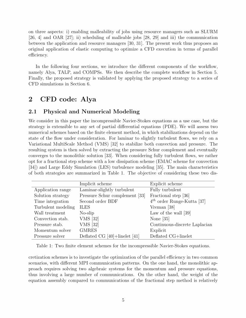
cretization schemes is to investigate the optimization of the parallel efficiency in two commonscenarios, with different MPI communication patterns. On the one hand, the monolithic ap-proach requires solving two algebraic systems for the momentum and pressure equations,thus involving a large number of communications. On the other hand, the weight of theequation assembly compared to communications of the fractional step method is relatively

5

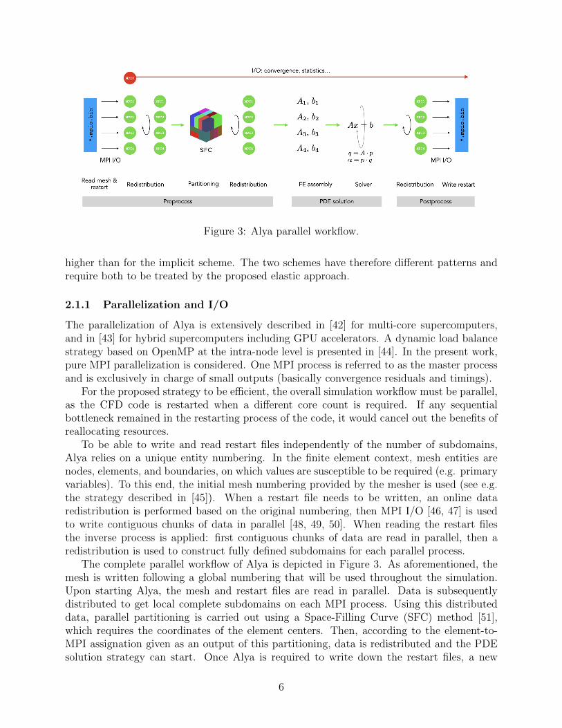
Figure 3: Alya parallel workflow.

higher than for the implicit scheme. The two schemes have therefore different patterns andrequire both to be treated by the proposed elastic approach.

2.1.1 Parallelization and I/O

The parallelization of Alya is extensively described in [42] for multi-core supercomputers,and in [43] for hybrid supercomputers including GPU accelerators. A dynamic load balancestrategy based on OpenMP at the intra-node level is presented in [44]. In the present work,pure MPI parallelization is considered. One MPI process is referred to as the master processand is exclusively in charge of small outputs (basically convergence residuals and timings).

For the proposed strategy to be efficient, the overall simulation workflow must be parallel,as the CFD code is restarted when a different core count is required. If any sequentialbottleneck remained in the restarting process of the code, it would cancel out the benefits ofreallocating resources.

To be able to write and read restart files independently of the number of subdomains,Alya relies on a unique entity numbering. In the finite element context, mesh entities arenodes, elements, and boundaries, on which values are susceptible to be required (e.g. primaryvariables). To this end, the initial mesh numbering provided by the mesher is used (see e.g.the strategy described in [45]). When a restart file needs to be written, an online dataredistribution is performed based on the original numbering, then MPI I/O [46, 47] is usedto write contiguous chunks of data in parallel [48, 49, 50]. When reading the restart filesthe inverse process is applied: first contiguous chunks of data are read in parallel, then aredistribution is used to construct fully defined subdomains for each parallel process.

The complete parallel workflow of Alya is depicted in Figure 3. As aforementioned, themesh is written following a global numbering that will be used throughout the simulation.Upon starting Alya, the mesh and restart files are read in parallel. Data is subsequentlydistributed to get local complete subdomains on each MPI process. Using this distributeddata, parallel partitioning is carried out using a Space-Filling Curve (SFC) method [51],which requires the coordinates of the element centers. Then, according to the element-to-MPI assignation given as an output of this partitioning, data is redistributed and the PDEsolution strategy can start. Once Alya is required to write down the restart files, a new

6

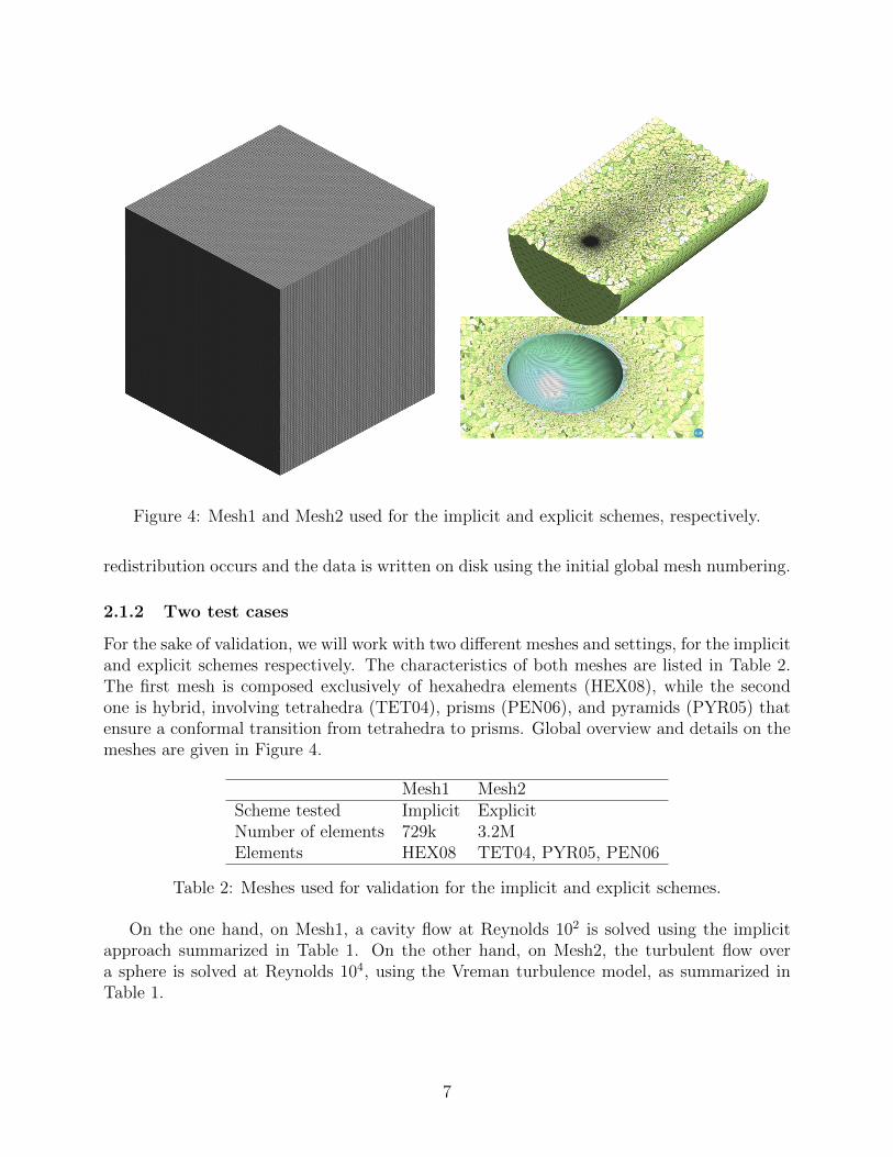
Figure 4: Mesh1 and Mesh2 used for the implicit and explicit schemes, respectively.

redistribution occurs and the data is written on disk using the initial global mesh numbering.

2.1.2 Two test cases

For the sake of validation, we will work with two different meshes and settings, for the implicitand explicit schemes respectively. The characteristics of both meshes are listed in Table 2.The first mesh is composed exclusively of hexahedra elements (HEX08), while the secondone is hybrid, involving tetrahedra (TET04), prisms (PEN06), and pyramids (PYR05) thatensure a conformal transition from tetrahedra to prisms. Global overview and details on themeshes are given in Figure 4.

Mesh1 Mesh2Scheme tested Implicit ExplicitNumber of elements 729k 3.2MElements HEX08 TET04, PYR05, PEN06

Table 2: Meshes used for validation for the implicit and explicit schemes.

On the one hand, on Mesh1, a cavity flow at Reynolds 102 is solved using the implicitapproach summarized in Table 1. On the other hand, on Mesh2, the turbulent flow overa sphere is solved at Reynolds 104, using the Vreman turbulence model, as summarized inTable 1.

7

3 Measuring Parallel Efficiency: TALP

The CFD code Alya relies on the library TALP to measure at runtime the parallel efficiencyof the simulation. We now explain in detail how TALP works and the different metrics itmeasures and can provide to Alya.

3.1 The library

TALP [3] is a lightweight and scalable tool for online parallel performance measurementintegrated within the Dynamic Load Balancing Library (DLB) [52, 53] library. DLB is aframework that aims at improving the performance of parallel applications and is designedin a modular way. It is transparent and non-intrusive for the application and user, and it isintegrated with MPI, OpenMP [54] and OMPSs API’s [55].

DLB includes three modules independent but coordinated and compatible:

• LeWI (Lend When Idle): provides a dynamic load balancing algorithm for hybridapplications.

• DROM (Dynamic Resource Ownership Management): offers a mechanism for dynamicresource management.

• TALP (Tracking Application Low-level Performance): measures parallel efficiency atruntime.

The TALP module is a profiling tool that collects statistical information about the con-tribution of every thread and process to the application execution. The tool measures loadimbalance and communication efficiency by profiling each of the supported parallel program-ming models. These performance measures can be obtained at runtime through the use ofan API, as well as from a post-mortem report. In the current work, we take advantage of theAPI offered to collect efficiency metrics at runtime. The measures done by TALP are basedon defining two main states for a running process: useful work and communication. Basedon these measures, it can provide parallel efficiency metrics as defined by the PoP centre ofexcellence [56, 57, 19].

By adding the required calls inside Alya through the API, we are thus able to obtain theperformance measurements during its execution (see Section 3.3). Then, according to theefficiency values inquired by Alya, resources will be adjusted to fulfill an efficiency criterion.

3.2 Efficiency Metrics

In this section, we explain the way the efficiency metrics are computed based on the profilingmeasurements. As mentioned previously, we simplify the status of a process into two states,namely useful work and communication. Figure 5 shows a graphical representation of twoprocesses running in parallel (p0 and p1) by coloring the two possible states.

In the HPC community, parallel efficiency is computed as the ratio between the usefulcomputation and the total consumed resources. Let us define tiw and tic the useful work

8

p0p1te Useful workCommunication

Parallel Efficiency = =+ te * PFigure 5: Graphical definition of Parallel Efficiency. P is the number of available cores andte the elapsed time.

and communication times of process i running on P cores. The total elapsed time te of anapplication is thus:

te = maxi

(tiw + tic). (1)

We also introduce tw as the total useful work time of the application:

tw =∑i

tiw.

Accordingly, the Parallel Efficiency (PE) can be computed as:

PE =tw

te × P

By using the PoP metrics, we divide the communication time into two separated metrics:

• Load Balance (LB): time spent waiting for the most loaded process to complete itstask.

• Communication Efficiency (CE): time spent in the MPI library, due to the inherentoverheads of communication.

Figure 6 shows a graphical representation of the difference between the two metrics.Based on this definition, they can be computed as:

CE =maxi(t

iw)

te, (2)

LB =tw

maxi(tiw)× P,

PE = LB × CE.

This difference is important because the approach to address a load balance issue isdifferent from the one to address a communication efficiency issue. On the one hand, a lowLB can be solved with a better domain partition or a dynamic load balancing mechanism.On the other hand, a low CE is usually an indicator that too many resources are used forthe current size of the problem. All the previous definitions are summarized in Table 3.

9

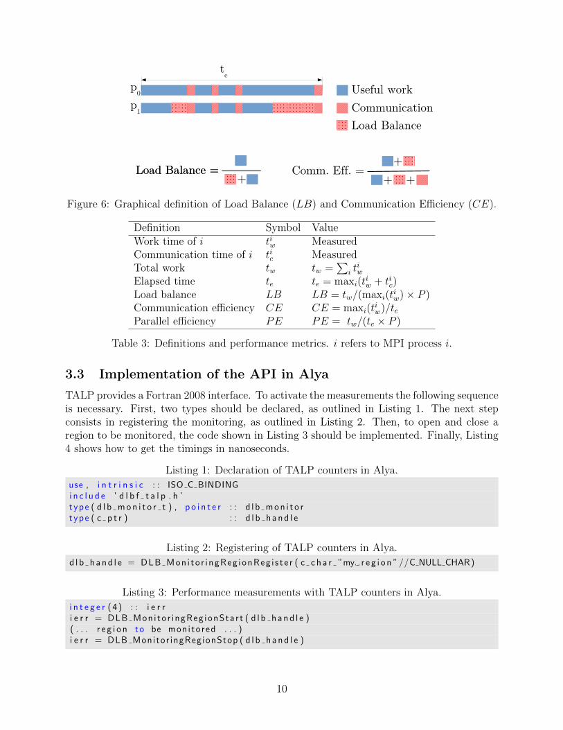
p0p1te Useful workCommunication Eff.Load Balance

Load Balance =Load Balance = + Comm. Eff. = ++ +Figure 6: Graphical definition of Load Balance (LB) and Communication Efficiency (CE).

Definition Symbol ValueWork time of i tiw MeasuredCommunication time of i tic MeasuredTotal work tw tw =

∑i t

iw

Elapsed time te te = maxi(tiw + tic)

Load balance LB LB = tw/(maxi(tiw)× P )

Communication efficiency CE CE = maxi(tiw)/te

Parallel efficiency PE PE = tw/(te × P )

Table 3: Definitions and performance metrics. i refers to MPI process i.

3.3 Implementation of the API in Alya

TALP provides a Fortran 2008 interface. To activate the measurements the following sequenceis necessary. First, two types should be declared, as outlined in Listing 1. The next stepconsists in registering the monitoring, as outlined in Listing 2. Then, to open and close aregion to be monitored, the code shown in Listing 3 should be implemented. Finally, Listing4 shows how to get the timings in nanoseconds.

Listing 1: Declaration of TALP counters in Alya.

use , i n t r i n s i c : : ISO C BINDINGi n c l u d e ’ d l b f t a l p . h ’t ype ( d l b mon i t o r t ) , p o i n t e r : : d l b mon i t o rtype ( c p t r ) : : d l b h a nd l e

Listing 2: Registering of TALP counters in Alya.

d l b h a nd l e = DLB Mon i to r i ngReg ionReg i s t e r ( c c h a r ”my r e g i o n ”//C NULL CHAR)

Listing 3: Performance measurements with TALP counters in Alya.

i n t e g e r (4 ) : : i e r ri e r r = DLB Mon i to r ingReg ionSta r t ( d l b h a nd l e )( . . . r e g i o n to be mon i to red . . . )i e r r = DLB Monitor ingRegionStop ( d l b h a nd l e )

10

Listing 4: Obtaining the TALP counters in Alya.

r e a l ( 8 ) : : e l a p s e d t im er e a l ( 8 ) : : accumulated MPI t imer e a l ( 8 ) : : accumulated comp t ime

c a l l c f p o i n t e r ( d l b hand l e , d l b mon i t o r )e l a p s e d t im e = r e a l ( d l b mon i t o r % e l ap s ed t ime , 8 )accumulated MPI t ime = r e a l ( d l b mon i t o r % accumulated MPI t ime , 8 )accumulated comp t ime = r e a l ( d l b mon i t o r % accumu la ted computa t i on t ime , 8 )

4 Workflow manager: COMPSs

We have just presented the CFD code and the library TALP to measure the performanceat runtime. We now briefly introduce the workflow manager, COMPSs. COMPSs [58] is atask-based programming model and runtime for simplifying the development and executionof parallel workflows in distributed computing environments. From an annotated sequen-tial code, the COMPSs runtime can detect data dependencies between the defined tasks’invocations, creating a task-dependency graph that allows the inference of the application’sinherent parallelism. Based on the required parallelism in each computation phase, theCOMPSs runtime interacts with the resource manager, such as SLURM, to adapt the com-putational resources to the application needs [59]. The dynamic job capability of SLURM,which allow us to increase or reduce the resources assigned to a job in execution, is describedin [60]. This feature ensures that new resources in the extended job are accessible by theProcess Management Interface (PMI) of MPI. This strategy can be easily implemented inother schedulers that provide a similar feature. If the scheduler does not provide this feature,COMPSs can also perform the scaling by adding new resources to the application throughstandard job submission. However, this option will only work if the scheduler allows startingan MPI application in resources from different jobs.

In the present case, COMPSs is used to implement and execute the optimization workflowthat orchestrates the Alya execution. The Alya executions are defined as COMPSs tasks. ACOMPSs workflow is defined to spawn the Alya computations collecting its resource require-ments through interaction with the resource manager and restarting the Alya execution withthe new resource configuration and the minimum downtime.

5 Optimization workflow: elastic computing

The overall workflow combines a CFD code Alya, a performance library TALP to measurethe communication efficiency CE, and a workflow manager COMPSs. The optimizationstrategy consists in adjusting the resources according to a measured performance criterion,the communication efficiency CE herein. In practice, the communication efficiency is inquiredby Alya to TALP at a given frequency, in terms of the number of time steps (e.g. each10 time steps), to have a representative average. Once measured, if CE falls outside aprescribed range, [CEmin, CEmax] (e.g. [0.8, 0.9]), then a new number of cores is estimatedand requested. The estimation of the number of cores will be described in Section 5.1.2.

11

5.1 Software strategy

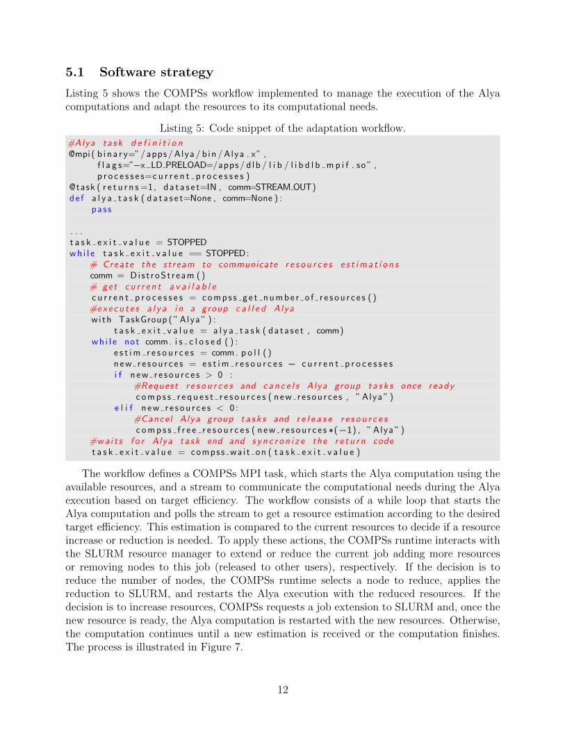
Listing 5 shows the COMPSs workflow implemented to manage the execution of the Alyacomputations and adapt the resources to its computational needs.

Listing 5: Code snippet of the adaptation workflow.

#Alya t a s k d e f i n i t i o n@mpi ( b i n a r y=”/ apps /Alya / b in /Alya . x” ,

f l a g s=”−x LD PRELOAD=/apps / d lb / l i b / l i b d l b m p i f . so ” ,p r o c e s s e s=c u r r e n t p r o c e s s e s )

@task ( r e t u r n s =1, d a t a s e t=IN , comm=STREAM OUT)de f a l y a t a s k ( d a t a s e t=None , comm=None ) :

pa s s

. . .t a s k e x i t v a l u e = STOPPEDwh i l e t a s k e x i t v a l u e == STOPPED:

# Create the st ream to communicate r e s o u r c e s e s t im a t i o n scomm = Dis t roS t r eam ( )# get c u r r e n t a v a i l a b l ec u r r e n t p r o c e s s e s = comps s g e t numbe r o f r e s o u r c e s ( )#exe cu t e s a l y a i n a group c a l l e d Alyawith TaskGroup ( ”Alya ” ) :

t a s k e x i t v a l u e = a l y a t a s k ( da ta s e t , comm)wh i l e not comm. i s c l o s e d ( ) :

e s t im r e s o u r c e s = comm. p o l l ( )n ew r e s ou r c e s = e s t im r e s o u r c e s − c u r r e n t p r o c e s s e si f n ew r e s ou r c e s > 0 :

#Request r e s o u r c e s and c a n c e l s Alya group t a s k s once readyc omp s s r e q u e s t r e s o u r c e s ( new re sou r c e s , ”Alya ” )

e l i f n ew r e s ou r c e s < 0 :#Cance l Alya group t a s k s and r e l e a s e r e s o u r c e sc omp s s f r e e r e s o u r c e s ( n ew r e s ou r c e s ∗(−1) , ”Alya ” )

#wa i t s f o r Alya t a s k end and s y n c r o n i z e the r e t u r n codet a s k e x i t v a l u e = compss wa i t on ( t a s k e x i t v a l u e )

The workflow defines a COMPSs MPI task, which starts the Alya computation using theavailable resources, and a stream to communicate the computational needs during the Alyaexecution based on target efficiency. The workflow consists of a while loop that starts theAlya computation and polls the stream to get a resource estimation according to the desiredtarget efficiency. This estimation is compared to the current resources to decide if a resourceincrease or reduction is needed. To apply these actions, the COMPSs runtime interacts withthe SLURM resource manager to extend or reduce the current job adding more resourcesor removing nodes to this job (released to other users), respectively. If the decision is toreduce the number of nodes, the COMPSs runtime selects a node to reduce, applies thereduction to SLURM, and restarts the Alya execution with the reduced resources. If thedecision is to increase resources, COMPSs requests a job extension to SLURM and, once thenew resource is ready, the Alya computation is restarted with the new resources. Otherwise,the computation continues until a new estimation is received or the computation finishes.The process is illustrated in Figure 7.

12

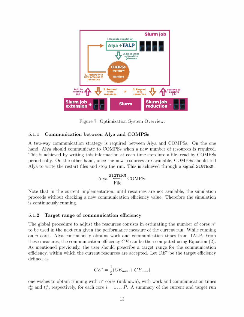
Figure 7: Optimization System Overview.

5.1.1 Communication between Alya and COMPSs

A two-way communication strategy is required between Alya and COMPSs. On the onehand, Alya should communicate to COMPSs when a new number of resources is required.This is achieved by writing this information at each time step into a file, read by COMPSsperiodically. On the other hand, once the new resources are available, COMPSs should tellAlya to write the restart files and stop the run. This is achieved through a signal SIGTERM:

AlyaSIGTERM−→←−File

COMPSs

Note that in the current implementation, until resources are not available, the simulationproceeds without checking a new communication efficiency value. Therefore the simulationis continuously running.

5.1.2 Target range of communication efficiency

The global procedure to adjust the resources consists in estimating the number of cores n∗

to be used in the next run given the performance measure of the current run. While runningon n cores, Alya continuously obtains work and communication times from TALP. Fromthese measures, the communication efficiency CE can be then computed using Equation (2).As mentioned previously, the user should prescribe a target range for the communicationefficiency, within which the current resources are accepted. Let CE∗ be the target efficiencydefined as

CE∗ =1

2(CEmin + CEmax)

one wishes to obtain running with n∗ cores (unknown), with work and communication timesti∗w and ti∗c , respectively, for each core i = 1 . . . P . A summary of the current and target run

13

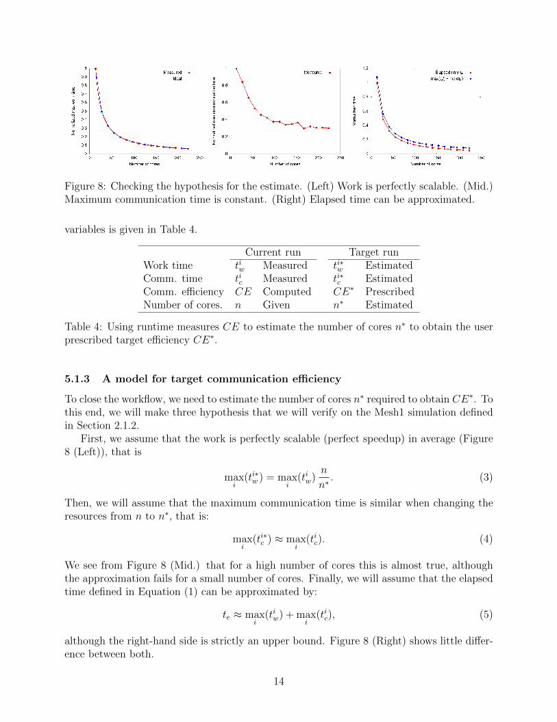
Figure 8: Checking the hypothesis for the estimate. (Left) Work is perfectly scalable. (Mid.)Maximum communication time is constant. (Right) Elapsed time can be approximated.

variables is given in Table 4.

Current run Target runWork time tiw Measured ti∗w EstimatedComm. time tic Measured ti∗c EstimatedComm. efficiency CE Computed CE∗ PrescribedNumber of cores. n Given n∗ Estimated

Table 4: Using runtime measures CE to estimate the number of cores n∗ to obtain the userprescribed target efficiency CE∗.

5.1.3 A model for target communication efficiency

To close the workflow, we need to estimate the number of cores n∗ required to obtain CE∗. Tothis end, we will make three hypothesis that we will verify on the Mesh1 simulation definedin Section 2.1.2.

First, we assume that the work is perfectly scalable (perfect speedup) in average (Figure8 (Left)), that is

maxi

(ti∗w ) = maxi

(tiw)n

n∗ . (3)

Then, we will assume that the maximum communication time is similar when changing theresources from n to n∗, that is:

maxi

(ti∗c ) ≈ maxi

(tic). (4)

We see from Figure 8 (Mid.) that for a high number of cores this is almost true, althoughthe approximation fails for a small number of cores. Finally, we will assume that the elapsedtime defined in Equation (1) can be approximated by:

te ≈ maxi

(tiw) + maxi

(tic), (5)

although the right-hand side is strictly an upper bound. Figure 8 (Right) shows little differ-ence between both.

14

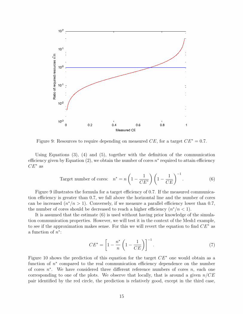
Figure 9: Resources to require depending on measured CE, for a target CE∗ = 0.7.

Using Equations (3), (4) and (5), together with the definition of the communicationefficiency given by Equation (2), we obtain the number of cores n∗ required to attain efficiencyCE∗ as

Target number of cores: n∗ = n

(1− 1

CE∗

)(1− 1

CE

)−1

. (6)

Figure 9 illustrates the formula for a target efficiency of 0.7. If the measured communica-tion efficiency is greater than 0.7, we fall above the horizontal line and the number of corescan be increased (n∗/n > 1). Conversely, if we measure a parallel efficiency lower than 0.7,the number of cores should be decreased to reach a higher efficiency (n∗/n < 1).

It is assumed that the estimate (6) is used without having prior knowledge of the simula-tion communication properties. However, we will test it in the context of the Mesh1 example,to see if the approximation makes sense. For this we will revert the equation to find CE∗ asa function of n∗:

CE∗ =

[1− n∗

n

(1− 1

CE

)]−1

. (7)

Figure 10 shows the prediction of this equation for the target CE∗ one would obtain as afunction of n∗ compared to the real communication efficiency dependence on the numberof cores n∗. We have considered three different reference numbers of cores n, each onecorresponding to one of the plots. We observe that locally, that is around a given n/CEpair identified by the red circle, the prediction is relatively good, except in the third case,

15

Figure 10: Prediction of Equation (7) to guess what would be the target CE∗ for a givennumber of target cores n∗ compared to real measures. Three references for n have beenconsidered for the estimate.

for which a non-smooth dependence is measured. This suggests that the estimate should beapplied carefully without requiring too big changes to the number of cores.

5.1.4 Control parameters

In this section, we will give all the control parameters required to set up an elastic simulation.We already mentioned in Section 5.1.2 that the user should provide a target range. To obtainstable results on the communication efficiency (to avoid reacting to one-time events), westated in Section 5 that an averaging period would enable us to stabilize the predictions.Also, we have just seen in the previous section that it may be desirable to control the rate ofchange r of the number of cores to make Equation (6) valid. This rate of change limits thenumber of core n∗

e estimated by Equation (6) to:

n∗e

r< n∗ < n∗

e r

In addition, to control the effects of possible odd events, we will limit the range of thepossible number of cores, based on experience, on the system, and the available number ofcores. Also, a starting number of cores should be prescribed to start the first optimizationstep. Finally, a starting time step from which the measurements are activated will helpto avoid a warm-up behavior of the execution. The following list summarizes the controlparameters proposed in this work.

• Communication efficiency target range;

• Averaging period;

• Rate of change of number of cores;

• Minimum number of cores;

• Maximum number of cores;

• Initial number of cores;

• Starting time step.

16

5.1.5 Overheads

Let us comment on the possible overheads compared to a classical CFD simulation. In thecase of Alya, the overhead consists of restarting the CFD simulation. However, this restartingprocess is limited in terms of CPU time by the fully parallelized Alya workflow describedin Section 2.1.1. In addition, restarting is a common unavoidable operation carried out inCFD simulations to provide checkpointing, which costs is similar to the cost of a post-processoutput. Regarding the cost of a simulation, this extra cost can be neglected.

Apart from the CFD code itself, the workflow involves two additional ingredients, namelyTALP and COMPSs. On the one hand, TALP is integrated into Alya and tested regularlyby the Alya performance suite [61]. Overhead of a maximum of 3% is obtained, whichis reasonable given the potential gain expected by the workflow. On the other hand, theoverhead of invoking a remote task with PyCOMPSs is about 10ms, which is negligiblecompared with overall cost of a CFD simulation. An important overhead could be addedby the management of the elasticity. There are two cases to consider, when requesting newresources and when releasing them. When requesting new resources, COMPSs submits newjobs to queueing system to access the missing resources. The submission of the job will takesome milliseconds which can be also insignificant compared to the simulation time. However,the resource manager can take some time to provide the requested resources. To overcomethese overheads, the workflow keeps the CFD simulation running with the old configurationuntil the new resources are available. In the case of releasing resources, COMPSs restartsthe CFD with a smaller resource configuration and releases the other resources using theSLURM API which is performed asynchronously without adding extra overhead.

6 Results

We now present the optimization results for both the implicit and explicit schemes. All theruns have been executed on Minotauro supercomputer, located at Barcelona SupercomputingCenter. Minotauro’s current configuration is:

• 38 bullx R421-E4 servers, each server with:

– 2 Intel Xeon E5–2630 v3 (Haswell) 8-core processors, (each core at 2.4 GHz,andwith 20 MB L3 cache)

– Peak Performance: 250.94 TFlops

– 120 GB SSD (Solid State Disk) as local storage

– 1 PCIe 3.0 x8 8GT/s, Mellanox ConnectX®–3FDR 56 Gbit

– 4 Gigabit Ethernet ports.

• The operating system is RedHat Linux 6.7.

For the whole optimization campaign, we give the control parameters in tables. In thefigures, the shadowed rectangle indicates the target range; the blue line the number of cores,and the red line the measured communication efficiency. For all the simulations, the minimumnumber of cores is set to 15, equivalent to one node of the system, while the maximum number

17

of cores is set to 240, equivalent to 16 nodes (we have found higher efficiencies using 15 coresper node instead of 16).

6.1 Implicit scheme

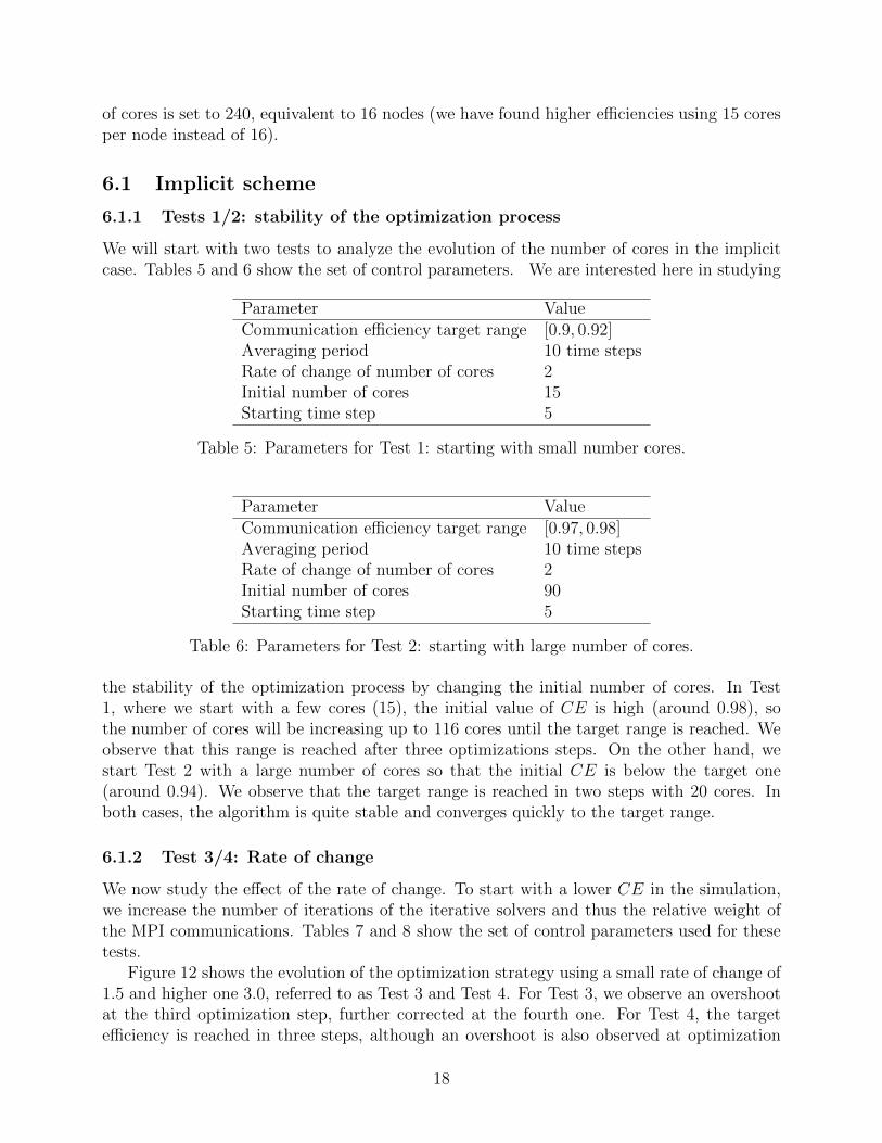
6.1.1 Tests 1/2: stability of the optimization process

We will start with two tests to analyze the evolution of the number of cores in the implicitcase. Tables 5 and 6 show the set of control parameters. We are interested here in studying

Parameter ValueCommunication efficiency target range [0.9, 0.92]Averaging period 10 time stepsRate of change of number of cores 2Initial number of cores 15Starting time step 5

Table 5: Parameters for Test 1: starting with small number cores.


Table 6: Parameters for Test 2: starting with large number of cores.

the stability of the optimization process by changing the initial number of cores. In Test1, where we start with a few cores (15), the initial value of CE is high (around 0.98), sothe number of cores will be increasing up to 116 cores until the target range is reached. Weobserve that this range is reached after three optimizations steps. On the other hand, westart Test 2 with a large number of cores so that the initial CE is below the target one(around 0.94). We observe that the target range is reached in two steps with 20 cores. Inboth cases, the algorithm is quite stable and converges quickly to the target range.

6.1.2 Test 3/4: Rate of change

We now study the effect of the rate of change. To start with a lower CE in the simulation,we increase the number of iterations of the iterative solvers and thus the relative weight ofthe MPI communications. Tables 7 and 8 show the set of control parameters used for thesetests.

Figure 12 shows the evolution of the optimization strategy using a small rate of change of1.5 and higher one 3.0, referred to as Test 3 and Test 4. For Test 3, we observe an overshootat the third optimization step, further corrected at the fourth one. For Test 4, the targetefficiency is reached in three steps, although an overshoot is also observed at optimization

18

Figure 11: Optimization evolution in terms of CE and number of cores n along the timeintegration. (Left) Test 1: starting with a small number of cores. See Table 5. (Right) Test2: starting with a large number of cores. See Table 6.

Parameter ValueCommunication efficiency target range [0.82, 0.86]Averaging period 10 time stepsRate of change of number of cores 1.5Initial number of cores 15Starting time step 10

Table 7: Parameters for Test 3: Rate of change.


Table 8: Parameters for Test 4: rate of change.

19

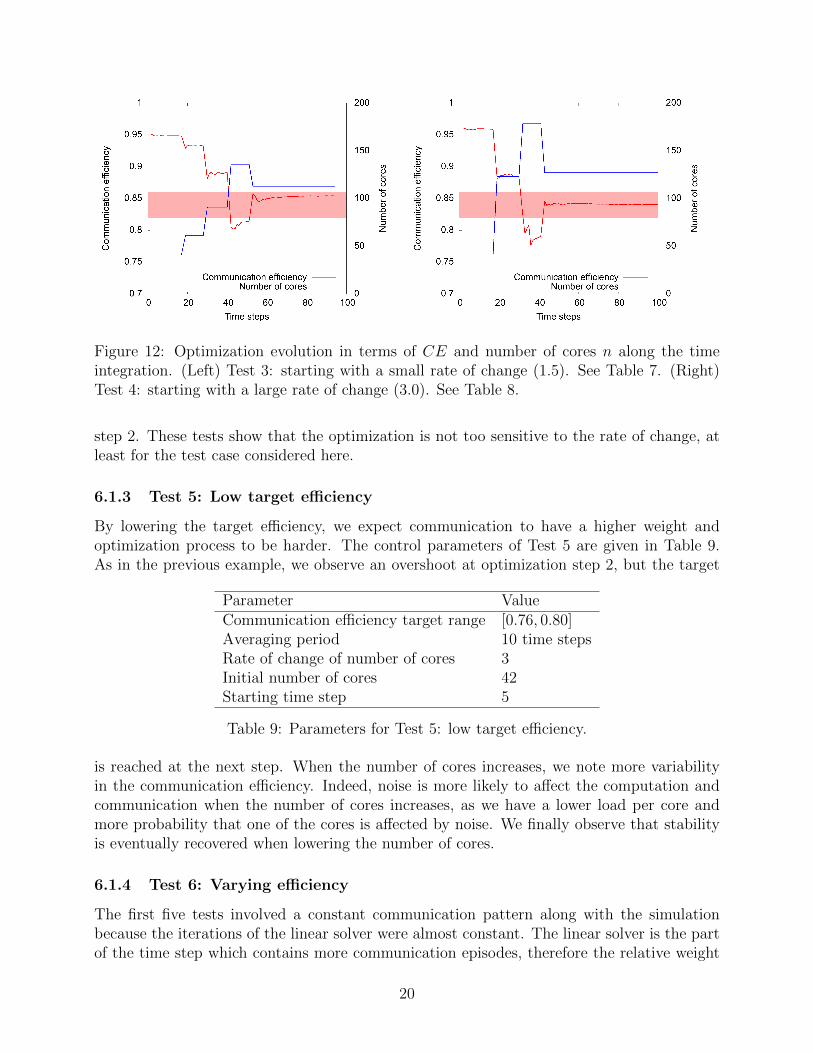
Figure 12: Optimization evolution in terms of CE and number of cores n along the timeintegration. (Left) Test 3: starting with a small rate of change (1.5). See Table 7. (Right)Test 4: starting with a large rate of change (3.0). See Table 8.

step 2. These tests show that the optimization is not too sensitive to the rate of change, atleast for the test case considered here.

6.1.3 Test 5: Low target efficiency

By lowering the target efficiency, we expect communication to have a higher weight andoptimization process to be harder. The control parameters of Test 5 are given in Table 9.As in the previous example, we observe an overshoot at optimization step 2, but the target


Table 9: Parameters for Test 5: low target efficiency.

is reached at the next step. When the number of cores increases, we note more variabilityin the communication efficiency. Indeed, noise is more likely to affect the computation andcommunication when the number of cores increases, as we have a lower load per core andmore probability that one of the cores is affected by noise. We finally observe that stabilityis eventually recovered when lowering the number of cores.

6.1.4 Test 6: Varying efficiency

The first five tests involved a constant communication pattern along with the simulationbecause the iterations of the linear solver were almost constant. The linear solver is the partof the time step which contains more communication episodes, therefore the relative weight

20

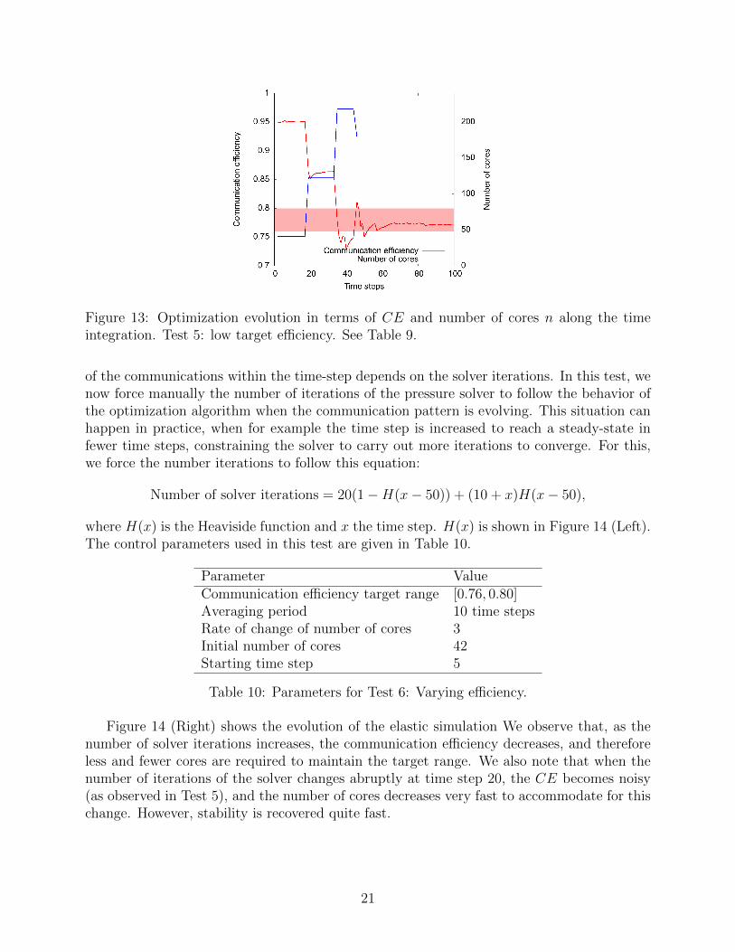
Figure 13: Optimization evolution in terms of CE and number of cores n along the timeintegration. Test 5: low target efficiency. See Table 9.

of the communications within the time-step depends on the solver iterations. In this test, wenow force manually the number of iterations of the pressure solver to follow the behavior ofthe optimization algorithm when the communication pattern is evolving. This situation canhappen in practice, when for example the time step is increased to reach a steady-state infewer time steps, constraining the solver to carry out more iterations to converge. For this,we force the number iterations to follow this equation:

Number of solver iterations = 20(1−H(x− 50)) + (10 + x)H(x− 50),

where H(x) is the Heaviside function and x the time step. H(x) is shown in Figure 14 (Left).The control parameters used in this test are given in Table 10.


Table 10: Parameters for Test 6: Varying efficiency.

Figure 14 (Right) shows the evolution of the elastic simulation We observe that, as thenumber of solver iterations increases, the communication efficiency decreases, and thereforeless and fewer cores are required to maintain the target range. We also note that when thenumber of iterations of the solver changes abruptly at time step 20, the CE becomes noisy(as observed in Test 5), and the number of cores decreases very fast to accommodate for thischange. However, stability is recovered quite fast.

21

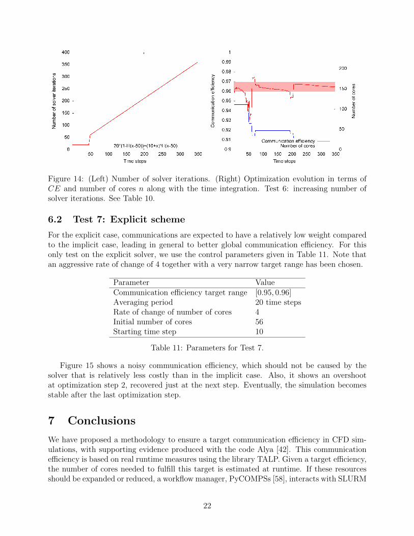
Figure 14: (Left) Number of solver iterations. (Right) Optimization evolution in terms ofCE and number of cores n along with the time integration. Test 6: increasing number ofsolver iterations. See Table 10.

6.2 Test 7: Explicit scheme

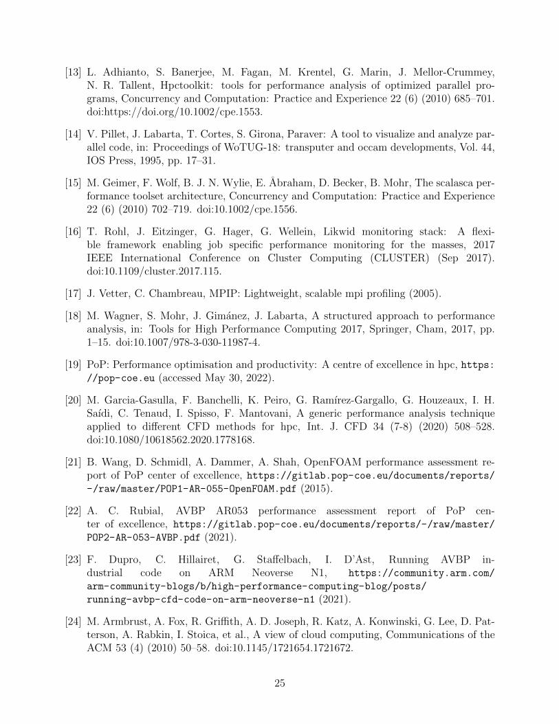
For the explicit case, communications are expected to have a relatively low weight comparedto the implicit case, leading in general to better global communication efficiency. For thisonly test on the explicit solver, we use the control parameters given in Table 11. Note thatan aggressive rate of change of 4 together with a very narrow target range has been chosen.


Table 11: Parameters for Test 7.

Figure 15 shows a noisy communication efficiency, which should not be caused by thesolver that is relatively less costly than in the implicit case. Also, it shows an overshootat optimization step 2, recovered just at the next step. Eventually, the simulation becomesstable after the last optimization step.

7 Conclusions

We have proposed a methodology to ensure a target communication efficiency in CFD sim-ulations, with supporting evidence produced with the code Alya [42]. This communicationefficiency is based on real runtime measures using the library TALP. Given a target efficiency,the number of cores needed to fulfill this target is estimated at runtime. If these resourcesshould be expanded or reduced, a workflow manager, PyCOMPSs [58], interacts with SLURM

22

Figure 15: (Left) Optimization evolution in terms of CE and number of cores n along withthe time integration. Test 7: explicit scheme. See Table 11.

to provide the new amount of cores to the simulation, while remaining inside the same job.When these resources are available, the CFD code is restarted and the simulation continues.

The optimization workflow proposed has been validated under different situations, userrequirements, and numerical methods, and has shown that the optimum partition is obtainedin very few optimization steps. We would like to eventually stress that, as a side effect,the methodology proposed provides resilience to the simulation workflow: if the simulationcrashes for any reason, it can be resumed with the remaining available resources.

As future work, we propose to understand the behavior of the workflow with more complexcases, where the communication efficiency patterns change during the iterations. In addition,it would be interesting to consider other target criteria, for example, the time-to-solutionregardless of the communication efficiency. This option would be useful for urgent computing,attaching computing resources to the simulation as they become available. Finally, theestimate for the target number of cores could be refined, for example considering the measuresfrom previous optimization steps.

Acknowledgements

This work has been supported by the Spanish Government (Grant PID2019-107255GB-C21by MCIN/AEI/ 10.13039/501100011033); by Generalitat de Catalunya (contract 2014-SGR-1051); by the European Commission H2020 project PoP CoE (GA n. 824080); by the Euro-pean Commission H2020 project CompBioMed CoE (GA n. 823712) and by the EuropeanCommission and the EuroHPC JU under contract 955558 (eFlows4HPC project).

References

[1] MPI: A message-passing interface standard version 3.0, http://mpi-forum.org/docs/mpi-3.0/mpi30-report.pdf.

23

[2] W. Lioen, M. Avillez, V. Codreanu, D. D. (GRNET), S. Dolas, A. Emerson, J. Finken-rath, C. Jourdain, M. Louhivuori, C. Morales, C. Moulinec, A. Proeme, A. Sunderland,Evaluation of accelerated and non-accelerated benchmarks, Deliverable 7.5, PRACE(2019).

[3] V. Lopez, G. Ramirez Miranda, M. Garcia-Gasulla, Talp: A lightweight tool to un-veil parallel efficiency of large-scale executions, in: Proceedings of the 2021 on Perfor-mance EngineeRing, Modelling, Analysis, and VisualizatiOn STrategy, 2021, pp. 3–10.doi:10.1145/3452412.3462753.

[4] SLURM: workload manager, https://slurm.schedmd.com/documentation.html.

[5] C.-H. Hsu, W.-C. Feng, A power-aware run-time system for high-performance comput-ing, in: SC ’05: Proceedings of the 2005 ACM/IEEE Conference on Supercomputing,2005, pp. 1–1. doi:10.1109/SC.2005.3.

[6] L. Riha, M. Merta, R. Vavrik, T. Brzobohaty, A. Markopoulos, O. Meca,O. Vysocky, T. Kozubek, V. Vondrak, A massively parallel and memory-efficientfem toolbox with a hybrid total feti solver with accelerator support, The Interna-tional Journal of High Performance Computing Applications 33 (4) (2019) 660–677.doi:10.1177/1094342018798452.

[7] O. Vysocky, M. Beseda, L. Rıha, J. Zapletal, M. Lysaght, V. Kannan, Meric and radargenerator: Tools for energy evaluation and runtime tuning of hpc applications, in:T. Kozubek, M. Cermak, P. Tichy, R. Blaheta, J. Sıstek, D. Lukas, J. Jaros (Eds.),High Performance Computing in Science and Engineering, Springer International Pub-lishing, Cham, 2018, pp. 144–159.

[8] N. Kappiah, V. Freeh, D. Lowenthal, Just in time dynamic voltage scaling: Exploitinginter-node slack to save energy in mpi programs, in: SC ’05: Proceedings of the 2005ACM/IEEE Conference on Supercomputing, 2005, pp. 33–33. doi:10.1109/SC.2005.39.

[9] Domain Knowledge Specification for Energy Tuning, Zenodo, 2017.doi:10.5281/zenodo.815852.

[10] V. Kannan, R. Borrell, M. Doyle, G. Houzeaux, Tuning alya for energy efficiency withreadex (2019). doi:10.5281/zenodo.2808081.

[11] Extrae: generating paraver trace-files for a post-mortem analysis, https://tools.bsc.es/extrae (2021).

[12] A. Knupfer, C. Rossel, D. a. Mey, S. Biersdorff, K. Diethelm, D. Eschweiler, M. Geimer,M. Gerndt, D. Lorenz, A. Malony, W. E. Nagel, Y. Oleynik, P. Philippen, P. Saviankou,D. Schmidl, S. Shende, R. Tschuter, M. Wagner, B. Wesarg, F. Wolf, Score-p: A jointperformance measurement run-time infrastructure for periscope, scalasca, tau, and vam-pir, in: H. Brunst, M. S. Muller, W. E. Nagel, M. M. Resch (Eds.), Tools for HighPerformance Computing 2011, Springer Berlin Heidelberg, Berlin, Heidelberg, 2012, pp.79–91.

24

[13] L. Adhianto, S. Banerjee, M. Fagan, M. Krentel, G. Marin, J. Mellor-Crummey,N. R. Tallent, Hpctoolkit: tools for performance analysis of optimized parallel pro-grams, Concurrency and Computation: Practice and Experience 22 (6) (2010) 685–701.doi:https://doi.org/10.1002/cpe.1553.

[14] V. Pillet, J. Labarta, T. Cortes, S. Girona, Paraver: A tool to visualize and analyze par-allel code, in: Proceedings of WoTUG-18: transputer and occam developments, Vol. 44,IOS Press, 1995, pp. 17–31.

[15] M. Geimer, F. Wolf, B. J. N. Wylie, E. Abraham, D. Becker, B. Mohr, The scalasca per-formance toolset architecture, Concurrency and Computation: Practice and Experience22 (6) (2010) 702–719. doi:10.1002/cpe.1556.

[16] T. Rohl, J. Eitzinger, G. Hager, G. Wellein, Likwid monitoring stack: A flexi-ble framework enabling job specific performance monitoring for the masses, 2017IEEE International Conference on Cluster Computing (CLUSTER) (Sep 2017).doi:10.1109/cluster.2017.115.

[17] J. Vetter, C. Chambreau, MPIP: Lightweight, scalable mpi profiling (2005).

[18] M. Wagner, S. Mohr, J. Gimanez, J. Labarta, A structured approach to performanceanalysis, in: Tools for High Performance Computing 2017, Springer, Cham, 2017, pp.1–15. doi:10.1007/978-3-030-11987-4.

[19] PoP: Performance optimisation and productivity: A centre of excellence in hpc, https://pop-coe.eu (accessed May 30, 2022).

[20] M. Garcia-Gasulla, F. Banchelli, K. Peiro, G. Ramırez-Gargallo, G. Houzeaux, I. H.Saıdi, C. Tenaud, I. Spisso, F. Mantovani, A generic performance analysis techniqueapplied to different CFD methods for hpc, Int. J. CFD 34 (7-8) (2020) 508–528.doi:10.1080/10618562.2020.1778168.

[21] B. Wang, D. Schmidl, A. Dammer, A. Shah, OpenFOAM performance assessment re-port of PoP center of excellence, https://gitlab.pop-coe.eu/documents/reports/-/raw/master/POP1-AR-055-OpenFOAM.pdf (2015).

[22] A. C. Rubial, AVBP AR053 performance assessment report of PoP cen-ter of excellence, https://gitlab.pop-coe.eu/documents/reports/-/raw/master/

POP2-AR-053-AVBP.pdf (2021).

[23] F. Dupro, C. Hillairet, G. Staffelbach, I. D’Ast, Running AVBP in-dustrial code on ARM Neoverse N1, https://community.arm.com/

arm-community-blogs/b/high-performance-computing-blog/posts/

running-avbp-cfd-code-on-arm-neoverse-n1 (2021).

[24] M. Armbrust, A. Fox, R. Griffith, A. D. Joseph, R. Katz, A. Konwinski, G. Lee, D. Pat-terson, A. Rabkin, I. Stoica, et al., A view of cloud computing, Communications of theACM 53 (4) (2010) 50–58. doi:10.1145/1721654.1721672.

25

[25] C. Qu, R. N. Calheiros, R. Buyya, Auto-scaling web applications in clouds: A taxonomyand survey, ACM Computing Surveys (CSUR) 51 (4) (2018) 1–33. doi:10.1145/3148149.

[26] A. B. Yoo, M. A. Jette, M. Grondona, SLURM: Simple linux utility for resource man-agement, in: Workshop on job scheduling strategies for parallel processing, Springer,2003, pp. 44–60.

[27] OAR, a versatile resource and task manager (also called a batch scheduler) for hpcclusters, https://oar.imag.fr.

[28] D. Fotakis, J. Matuschke, O. Papadigenopoulos, Malleable Scheduling Beyond Identi-cal Machines, in: D. Achlioptas, L. A. Vegh (Eds.), Approximation, Randomization,and Combinatorial Optimization. Algorithms and Techniques (APPROX/RANDOM2019), Vol. 145 of Leibniz International Proceedings in Informatics (LIPIcs), SchlossDagstuhl–Leibniz-Zentrum fuer Informatik, Dagstuhl, Germany, 2019, pp. 17:1–17:14.doi:10.4230/LIPIcs.APPROX-RANDOM.2019.17.

[29] K. Jansen, H. Zhang, An approximation algorithm for scheduling malleable tasks undergeneral precedence constraints, ACM Transactions on Algorithms (TALG) 2 (3) (2006)416–434. doi:10.1145/1159892.1159899.

[30] M. D’Amico, M. Garcia-Gasulla, V. Lopez, A. Jokanovic, R. Sirvent, J. Corbalan, Drom:Enabling efficient and effortless malleability for resource managers, in: Proceedings of the47th International Conference on Parallel Processing Companion, ICPP ’18, Associationfor Computing Machinery, New York, NY, USA, 2018. doi:10.1145/3229710.3229752.

[31] M. C. Cera, Y. Georgiou, O. Richard, N. Maillard, P. O. A. Navaux, Supporting mal-leability in parallel architectures with dynamic cpusetsmapping and dynamic MPI, in:K. Kant, S. V. Pemmaraju, K. M. Sivalingam, J. Wu (Eds.), Distributed Comput-ing and Networking, Springer Berlin Heidelberg, Berlin, Heidelberg, 2010, pp. 242–257.doi:10.1007/978-3-642-11322-2 26.

[32] G. Houzeaux, J. Principe, A variational subgrid scale model for transient incompressibleflows, Int. J. Comp. Fluid Dyn. 22 (3) (2008) 135–152. doi:10.1080/10618560701816387.

[33] G. Houzeaux, R. Aubry, M. Vazquez, Extension of fractional step techniques for incom-pressible flows: The preconditioned Orthomin(1) for the pressure Schur complement,Comput. Fluids 44 (2011) 297–313. doi:10.1016/j.compfluid.2011.01.017.

[34] S. Charnyi, T. Heister, M. A. Olshanskii, L. G. Rebholz, On conservation laws ofNavier–Stokes Galerkin discretizations, Journal of Computational Physics 337 (2017)289–308. doi:10.1016/j.jcp.2017.02.039.

[35] O. Lehmkuhl, G. Houzeaux, H. Owen, G. Chrysokentis, I. Rodrıguez, A low-dissipationfinite element scheme for scale resolving simulations of turbulent flows, J. Comp. Phys.390 (2019) 51–65. doi:10.1016/j.jcp.2019.04.004.

[36] R. Codina, Pressure stability in fractional step finite element methods for incompressibleflows, J. Comput. Phys. 170 (2001) 112–140. doi:10.1006/jcph.2001.6725.

26

[37] F. Capuano, G.Coppola, L. Randez, L. de Luca, Explicit Runge-Kutta schemes forincompressible flow with improved energy-conservation properties 328 (C) (2017).

[38] A. Vreman, An eddy-viscosity subgrid-scale model for turbulent shear flow: Al-gebraic theory and applications, Physics of Fluids 16 (10) (2004) 3670–3681.doi:10.1063/1.1785131.

[39] H. Owen, G. Chrysokentis, M. Avila, D. Mira, G. Houzeaux, J. Cajas, O. Lehmkuhl,Wall-modeled large-eddy simulation in a finite element framework, Int. J. Numer. Meth.Fluids 92 (2020) 20–37. doi:DOI: 10.1002/fld.4770.

[40] R. Lohner, F. Mut, J. Cebral, R. Aubry, G. Houzeaux, Deflated preconditioned conjugategradient solvers for the pressure-poisson equation: Extensions and improvements, Int.J. Num. Meth. Eng. 87 (2011) 2–14. doi:10.1002/nme.2932.

[41] O. Soto, R. Lohner, F. Camelli, A linelet preconditioner for incompressibleflow solvers, Int. J. Num. Meth. Heat Fluid Flow 13 (1) (2003) 133–147.doi:10.1108/09615530310456796.

[42] M. Vazquez, G. Houzeaux, S. Koric, A. Artigues, J. Aguado-Sierra, R. Arıs, D. Mira,H. Calmet, F. Cucchietti, H. Owen, A. Taha, E. D. Burness, J. M. Cela, M. Valero,Alya: Multiphysics engineering simulation towards exascale, J. Comput. Sci. 14 (2016)15–27. doi:10.1016/j.jocs.2015.12.007.

[43] R. Borrell, D. Dosimont, M. Garcia-Gasulla, G. Houzeaux, O. Lehmkuhl, V. Mehta,H. Owen, M. Vazquez, G. Oyarzun, Heterogeneous CPU/GPU co-execution of CFDsimulations on the Power9 architecture: Application to airplane aerodynamics, FutureGeneration Computer Systems 107 (2020) 31–48. doi:10.1016/j.future.2020.01.045.

[44] M. Garcia-Gasulla, G. Houzeaux, R. Ferrer, A. Artigues, V. Lopez, J. Labarta,M. Vazquez, MPI+ X: task-based parallelisation and dynamic load balance of finite el-ement assembly, International Journal of Computational Fluid Dynamics 33 (3) (2019)115–136. doi:10.1080/10618562.2019.1617856.

[45] Y. Fournier, Massively parallel location and exchange tools for unstructured meshes,International Journal of Computational Fluid Dynamics 34 (7-8) (2020) 549–568.doi:10.1080/10618562.2020.1810676.

[46] J.-P. Prost, MPI-IO, Springer US, Boston, MA, 2011, pp. 1191–1199. doi:10.1007/978-0-387-09766-4 297.

[47] P. Corbett, D. Feitelson, S. Fineberg, Y. Hsu, B. Nitzberg, J.-P. Prost, M. Snir,B. Traversat, P. Wong, Overview of the MPI-IO parallel I/O interface, Wiley-IEEEPress, 2001, pp. 477–487. doi:10.1109/9780470544839.ch32.

[48] Y. Fournier, J. Bonelle, E. L. Coupanec, A. Ribes, B. Lorendeau, C. Moulinec, Re-cent and upcoming changes in code Saturne: computational fluid dynamics HPC toolsoriented features, in: Proceedings of the Fourth International Conference on Parallel,

27

Distributed, Grid and Cloud Computing for Engineering, Dubrovnik, Croatia, 2015.doi:doi:10.4203/ccp.107.

[49] J. Kodavasal, K. Harmsa, P. Srivastavab, S. Soma, S. Quanb, K. Richards, M. Garcıa,Performance enhancement of an internal combustion engine CFD simulation on IBMBlue Gene/Q, in: ISC High Performance, Frankfurt (Germany), 2015.

[50] K. Jansen, M. Rasquin, J. Brown, C. Smith, M. Shephard, C. Carother, Exascale Scien-tific Applications: Scalability and Performance Portability, Chapman and Hall/CRC,2017, Ch. Extreme scale unstructured adaptive CFD for aerodynamic flow control.doi:10.1201/b21930.

[51] R. Borrell, J. Cajas, D. Mira, A. Taha, S. Koric, M. Vazquez, G. Houzeaux, Parallelmesh partitioning based on space filling curves, Comput. & Fluids 173 (2018) 264–272.doi:10.1016/j.compfluid.2018.01.040.

[52] M. Garcia, J. Corbalan, J. Labarta, LeWI: A runtime balancing algorithm for nestedparallelism, in: Proceedings of the International Conference on Parallel Processing(ICPP09), 2009. doi:10.1109/ICPP.2009.56.

[53] M. Garcia, J. Labarta, J. Corbalan, Hints to improve automatic load balancing withLeWi for hybrid applications, Journal of Parallel and Distributed Computing 74 (9)(2014) 2781 – 2794. doi:10.1016/j.jpdc.2014.05.004.

[54] OpenMP technical report 6: Version 5.0 preview 2, http://www.openmp.org/

wp-content/uploads/openmp-TR6.pdf (November 2017).

[55] A. Duran, E. Ayguade, R. Badia, J. Labarta, L. Martinell, X. Martorell, J. Planas,OMPSs: a proposal for programming heterogeneous multi-core architectures, ParallelProcessing Letters 21 (02) (2011) 173–193. doi:10.1142/S0129626411000151.

[56] M. Wagner, S. Mohr, J. Gimenez, J. Labarta, A structured approach to performanceanalysis, in: International Workshop on Parallel Tools for High Performance Computing,Springer, 2017, pp. 1–15. doi:10.1007/978-3-030-11987-4 1.

[57] F. Banchelli, K. Peiro, A. Querol, G. Ramirez-Gargallo, et al., Performance study ofhpc applications on an arm-based cluster using a generic efficiency model, in: 202028th Euromicro International Conference on Parallel, Distributed and Network-BasedProcessing (PDP), IEEE, 2020, pp. 167–174. doi:10.1109/PDP50117.2020.00032.

[58] R. M. Badia, J. Conejero, C. Diaz, J. Ejarque, D. Lezzi, F. Lordan, C. Ramon-Cortes,R. Sirvent, Comp superscalar, an interoperable programming framework, SoftwareX 3(2015) 32–36. doi:10.1016/j.softx.2015.10.004.

[59] F. Lordan, E. Tejedor, J. Ejarque, R. Rafanell, J. Alvarez, F. Marozzo, D. Lezzi, R. Sir-vent, D. Talia, R. M. Badia, Servicess: an interoperable programming framework for thecloud, Journal of Grid Computing 12 (1) (2014) 67–91. doi:10.1007/s10723-013-9272-5.

[60] SLURM FAQ, https://slurm.schedmd.com/faq.html#job_size (2021).

28

[61] Alya performance suite, https://rooster.bsc.es (November 2021).

29

Dynamic resource allocation for efficient parallel CFD ... - arXiv

Documents