Impact of Geomaterial Properties and Roller Parameters on ...

University of Texas at El Paso University of Texas at El Paso

ScholarWorks@UTEP ScholarWorks@UTEP

Open Access Theses & Dissertations

2021-07-01

Impact of Geomaterial Properties and Roller Parameters on Impact of Geomaterial Properties and Roller Parameters on

Intelligent Compaction Measurement Values Using Lumped Intelligent Compaction Measurement Values Using Lumped

Parameter Modeling Parameter Modeling

Jesús Castro Pérez University of Texas at El Paso

Follow this and additional works at: https://scholarworks.utep.edu/open_etd

Part of the Civil Engineering Commons

Recommended Citation Recommended Citation Castro Pérez, Jesús, "Impact of Geomaterial Properties and Roller Parameters on Intelligent Compaction Measurement Values Using Lumped Parameter Modeling" (2021). Open Access Theses & Dissertations. 3226. https://scholarworks.utep.edu/open_etd/3226

This is brought to you for free and open access by ScholarWorks@UTEP. It has been accepted for inclusion in Open Access Theses & Dissertations by an authorized administrator of ScholarWorks@UTEP. For more information, please contact [email protected].

IMPACT OF GEOMATERIAL PROPERTIES AND ROLLER PARAMETERS ON

INTELLIGENT COMPACTION MEASUREMENT VALUES USING

LUMPED PARAMETER MODELING

JESUS CASTRO PEREZ

Master’s Program in Civil Engineering

APPROVED:

___________________________________

Soheil Nazarian, Ph.D., Chair

___________________________________

Cesar Tirado, Ph.D.

___________________________________

Arturo Bronson, Ph.D.

___________________________________

Stephen L. Crites, Jr., Ph.D.

Dean of the Graduate School

IMPACT OF GEOMATERIAL PROPERTIES AND ROLLER PARAMETERS ON

INTELLIGENT COMPACTION MEASUREMENT VALUES USING

LUMPED PARAMETER MODELING

by

JESUS CASTRO PEREZ, BSCE

THESIS

Presented to the Faculty of the Graduate School of

The University of Texas at El Paso

in Partial fulfillment

of the Requirements

for the Degree of

MASTER OF SCIENCE

Department of Civil Engineering

THE UNIVERSITY OF TEXAS AT EL PASO

August 2021

iii

Acknowledgments

First, I want to thank my parents for their unconditional love, patience, and support during

my studies. My parents are the greatest blessing I have ever received. I am also grateful to my

sister, brother-in-law, and three beloved nieces for being my inspiration.

I want to express profound appreciation to my advisor Dr. Soheil Nazarian for the

opportunity to join the University of Texas at El Paso and work on this project. His patience and

advice were essential during my academic journey. Furthermore, I want to thank Dr. Cesar Tirado

for the lessons and time he provided to discuss my research and related concerns. I also thank Dr.

Arturo Bronson for accepting being part of my thesis committee. Additionally, I feel thankful to

Dr. Ivonne Santiago for allowing me to be the teaching assistant of her laboratory sessions. The

trust she always deposited in me had a massive meaning during all my studies.

Also, I am grateful to UTEP for allowing me to learn from incredible professors and meet

amazing people who later became friends. Last year was not easy, but it was enjoyable because of

the friends I made. Arahim Zuñiga, for all those cups of coffee, endless conversations, and

empathy, this work is also thanks to you. I would like to extend my gratitude to my friends Mariana

Benitez and Selene Fernandez for their encouragement to complete this thesis and unique coffee

recommendations, and to Carolina Hernandez for her time, constant motivation, and true

friendship.

Last but not least, I thank the City of El Paso for adopting me and bringing loving,

memorable, and welcoming people into my life.

iv

Abstract

Roads consist of layers of geomaterials and asphalt or concrete to provide an optimal

service life according to their exposure to traffic and the environment. Each layer that forms a

pavement structure requires achieving specific quality and mechanical properties that are often

obtained only through a proper compaction process.

Traditionally, compacted layers are tested using spot methods, which rely on the

assumption that the properties measured from a small sample of material represent an entire

section. This limitation has led to quality management techniques that continuously monitor the

acceleration records from a sensor installed on the roller's drum. These techniques are known as

Continuous Compaction Control (CCC) or Intelligent Compaction (IC), and their results are in

terms of Intelligent Compaction Measurement Values (ICMV).

This study aims at developing a model through Simscape (Matlab™) that simulates soil

compaction with a vibratory roller to characterize the relationships between the response of the

drum and the mechanical properties of the compacted geomaterial. Since different roller

manufacturers of IC rollers use different proprietary ICMV formulas, the Compaction Meter Value

(CMV) and Compaction Control Value (CCV) are used throughout this study. This document

summarizes the evaluation of changes in ICMV results from fluctuations in roller-specific

characteristics.

A sensitivity analysis was performed to evaluate the impact of individual soil properties

and roller parameters on the simulated CMV and CCV results. The overall results indicated that

CCV provides results less sensitive to changes in individual roller-specific parameters than CMV.

Additionally, CCV results maintained proportional values to simulated soil mechanical properties

in most simulated scenarios, while CMV did not.

v

Table of Contents

Acknowledgments.......................................................................................................................... iii

Abstract .......................................................................................................................................... iv

Table of Contents ............................................................................................................................ v

List of Tables ................................................................................................................................ vii

List of Figures .............................................................................................................................. viii

Chapter 1. Introduction ................................................................................................................... 1

1.1 Problem Statement ........................................................................................................... 1

1.2 Objective .......................................................................................................................... 2

1.3 Organization ..................................................................................................................... 2

Chapter 2. Literature Review .......................................................................................................... 3

2.1 Vibratory Roller Compaction ........................................................................................... 3

2.2 Review of Drum-Soil Interaction ..................................................................................... 4

2.3 Intelligent Compaction Measurement Values .................................................................. 6

2.3.1 Compaction Meter Value (CMV) ............................................................................. 7

2.3.2 Compaction Control Value (CCV) ........................................................................... 7

2.4 Numerical Modeling Techniques of Compacted Geomaterials ..................................... 10

2.5 Contact Force ................................................................................................................. 10

2.6 Summary ........................................................................................................................ 11

Chapter 3. Development of Lumped Parameter Model ................................................................ 13

3.1 Model Concept ............................................................................................................... 13

3.2 Numerical Model............................................................................................................ 16

3.3 Drum-Soil Interaction .................................................................................................... 19

3.4 Model Behavior .............................................................................................................. 20

3.5 Extraction of Mechanical Properties .............................................................................. 31

3.5.1 Secant Method ........................................................................................................ 31

3.5.2 FFT Method ............................................................................................................ 33

3.6 Estimation of Modulus ................................................................................................... 37

Chapter 4. Sensitivity Analysis, Results, and Discussion. ........................................................... 39

4.1. OAT Sensitivity Analysis Methodology ........................................................................ 39

vi

4.2 Geomaterial Mechanical Properties ............................................................................... 41

4.2.1 Soil Stiffness ........................................................................................................... 41

4.2.2 Soil Damping .......................................................................................................... 44

4.3 Static Weight .................................................................................................................. 46

4.3.1 Frame Mass ............................................................................................................. 46

4.3.2 Drum Mass .............................................................................................................. 48

4.3.3 Assumed Soil Mass ................................................................................................. 48

4.4 Frame-Drum Suspension System ................................................................................... 51

4.4.1 Frame-Drum Stiffness (KD-F) .................................................................................. 51

4.4.2 Frame-Drum Damping (CD-F) ................................................................................. 52

4.5 Eccentric Mass System................................................................................................... 54

4.5.1 Operating Frequency ............................................................................................... 54

4.5.2 Amplitude ............................................................................................................... 55

Chapter 5. Summary and Conclusions .......................................................................................... 57

5.1 Summary ........................................................................................................................ 57

5.2 Conclusions .................................................................................................................... 57

5.3 Recommendation for Future Work and Research .......................................................... 58

References ..................................................................................................................................... 60

LIST OF ACRONYMS, ABBREVIATIONS, AND SYMBOLS ............................................... 63

Appendix A ................................................................................................................................... 65

Vita ................................................................................................................................................ 70

vii

List of Tables

Table 1. Commercially available roller measurement values (Mooney et al., 2010) ..................... 8

Table 2. Literature review of intelligent compaction and lumped parameter models. ................. 12

Table 3. Description of input parameters in lumped model. ......................................................... 15

Table 4. Hard stop assumed parameters for roller-soil interaction simulation. ............................ 20

Table 5. Comparison of secant stiffness results vs model stiffness values. .................................. 32

Table 6. Comparison of FFT stiffness results vs. model stiffness values. .................................... 36

Table 7. Roller variable values for Sakai SV 510D ...................................................................... 39

Table 8. Parameter value ranges in commercially available vibratory rollers. ............................. 40

viii

List of Figures

Figure 1. Drum excitation mechanism inside a vibratory roller (Adam, 1996). ............................. 4

Figure 2. Observed modes of vibratory rollers interaction with soil .............................................. 5

Figure 3. (a) Acceleration record in the time domain. (b) Amplitude of acceleration in the

frequency domain (Mooney et al., 2010). ....................................................................................... 9

Figure 4. Amplitudes of acceleration in frequency domain used for CCV calculations (Mooney et

al., 2010; Scherocman et al., 2007). ................................................................................................ 9

Figure 5. 3DOF lumped parameter model (van Susante and Mooney, 2008). ............................. 11

Figure 6. (a) Vibratory roller lumped model with drum-soil contact. (b) Representation of lumped

model during a loss of contact. ..................................................................................................... 14

Figure 7. Lumped model, as observed in Simscape (Matlab). ...................................................... 16

Figure 8. Free-body diagram of frame mass. ................................................................................ 17

Figure 9. Free body diagram of drum attached the soil mass. ...................................................... 17

Figure 10. Forces acting on the spring-damper simulated soil during loss of contact. ................. 18

Figure 11. (a) Simple representation of Translational Hard Stop mechanism (b) Representation of

components in Translational Hard Stop used in lumped model. .................................................. 19

Figure 12. Sample model responses during continuous contact drum-soil interaction mode. ..... 21

Figure 13. Sample model responses during continuous contact drum-soil interaction mode in the

frequency domain.......................................................................................................................... 22

Figure 14. Sample model responses during partial uplift drum-soil interaction mode. ................ 23

Figure 15. Sample model responses during partial uplift drum-soil interaction mode. ................ 25

Figure 16. Sample model responses during double jump drum-soil interaction mode. ............... 26

Figure 17. Sample model responses during double jump drum-soil interaction mode. ............... 27

Figure 18. Sample model responses during “multiple” jump drum-soil interaction mode. ......... 28

Figure 19. Model behavior example with “multiple” jump drum-soil interaction mode. ............ 29

Figure 20. Sample of drum acceleration in the frequency domain for different drum-soil interaction

modes. ........................................................................................................................................... 30

Figure 21. Conceptual representation of Secant Stiffness during (a) continuous contact and (b) loss

of drum-soil contact (Mooney et al., 2010). ................................................................................. 31

Figure 22. Contact Force – Displacement Hysteresis Loops Samples generated by the same roller

at different soil stiffness values. .................................................................................................... 32

Figure 23. Contact force and drum displacement amplitudes during continuous contact mode. . 34

Figure 24. Contact force spectrum for different drum-soil interaction modes. ............................ 34

Figure 25. Drum displacement spectrum for different drum-soil interaction modes ................... 35

Figure 26. “FFT” Ks using drum and soil displacement records vs input Ks. ............................... 37

Figure 27. ICMVs (unitless) vs modeled soil stiffness (MN/m) .................................................. 42

Figure 28. Drum acceleration amplitudes vs. soil stiffness. ......................................................... 43

Figure 29. Drum-soil interaction modes on a CMV + CCV vs modeled soil stiffness plot. ....... 44

Figure 30. Impact of soil damping coefficient in CMV for five different soil stiffness values.... 45

ix

Figure 31. Impact of soil damping coefficient in CCV for five different soil stiffness values. ... 46

Figure 32. Impact of frame mass in CMV results for five Ks values. ........................................... 47

Figure 33. Impact of frame mass in CCV results for five Ks values. ............................................ 47

Figure 34. Impact of drum mass in CMV results for five Ks values. ............................................ 49

Figure 35. Impact of drum mass in CCV results for five Ks values. ............................................. 49

Figure 36. Impact of soil mass in CMV results for five Ks values. .............................................. 50

Figure 37. Impact of soil mass in CCV results for five Ks values. ............................................... 50

Figure 38. Impact of drum-frame suspension stiffness in CMV results for five Ks values. ......... 51

Figure 39. Impact of drum-frame suspension stiffness in CCV results for five Ks values. .......... 52

Figure 40. Impact of drum-frame suspension damping in CMV results for five Ks values. ......... 53

Figure 41. Impact of drum-frame suspension damping in CCV results for five Ks values. ......... 53

Figure 42. Impact of rotating frequency ( f ) in CMV results for five Ks values. ......................... 54

Figure 43. Impact of operational frequency ( f ) in CCV results for five Ks values. .................... 55

Figure 44. Impact of operational Amplitude (A) in CMV results for five Ks values. ................... 56

Figure 45. Impact of operational Amplitude (A) in CCV results for five Ks values. .................... 56

1

Chapter 1. Introduction

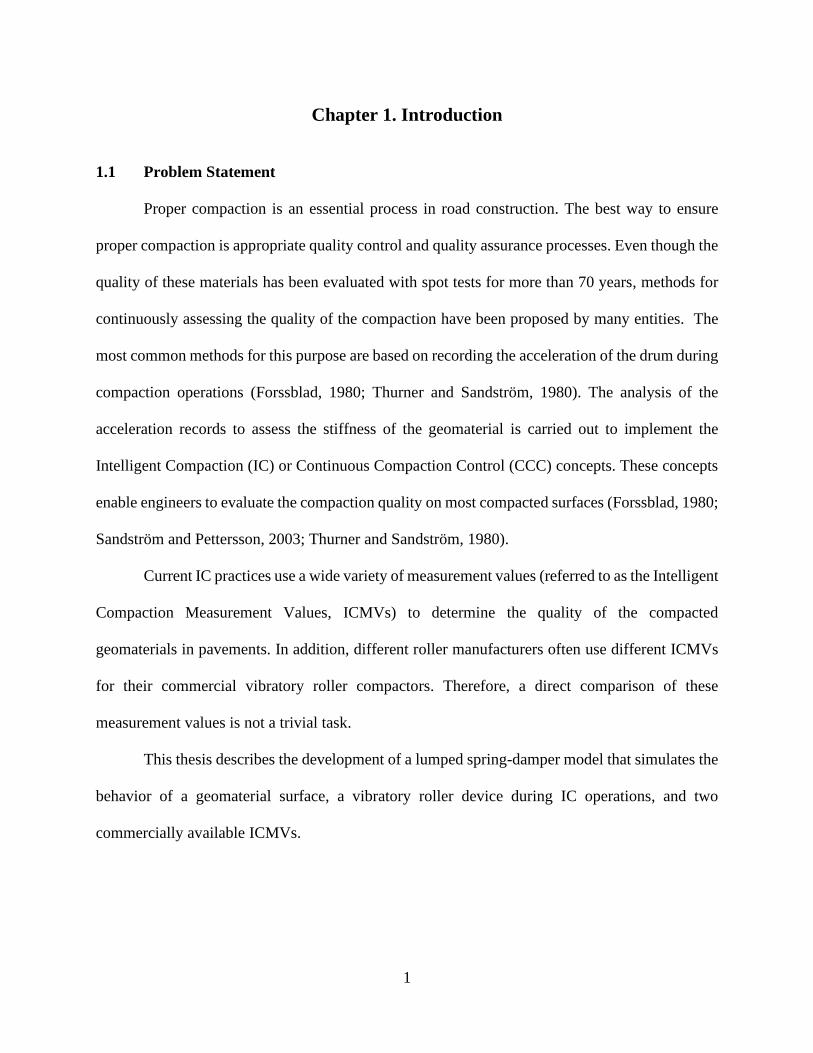
1.1 Problem Statement

Proper compaction is an essential process in road construction. The best way to ensure

proper compaction is appropriate quality control and quality assurance processes. Even though the

quality of these materials has been evaluated with spot tests for more than 70 years, methods for

continuously assessing the quality of the compaction have been proposed by many entities. The

most common methods for this purpose are based on recording the acceleration of the drum during

compaction operations (Forssblad, 1980; Thurner and Sandström, 1980). The analysis of the

acceleration records to assess the stiffness of the geomaterial is carried out to implement the

Intelligent Compaction (IC) or Continuous Compaction Control (CCC) concepts. These concepts

enable engineers to evaluate the compaction quality on most compacted surfaces (Forssblad, 1980;

Sandström and Pettersson, 2003; Thurner and Sandström, 1980).

Current IC practices use a wide variety of measurement values (referred to as the Intelligent

Compaction Measurement Values, ICMVs) to determine the quality of the compacted

geomaterials in pavements. In addition, different roller manufacturers often use different ICMVs

for their commercial vibratory roller compactors. Therefore, a direct comparison of these

measurement values is not a trivial task.

This thesis describes the development of a lumped spring-damper model that simulates the

behavior of a geomaterial surface, a vibratory roller device during IC operations, and two

commercially available ICMVs.

2

1.2 Objective

The objective of this thesis is to develop a model that simulates IC operations and evaluates

the impact of roller characteristics in estimating geomaterials properties, particularly stiffness and

ICMVs.

1.3 Organization

Aside from this chapter, this document is structured into seven chapters. Chapter 2 contains

a literature review of vibratory roller compaction, ICMV, and numerical modeling techniques used

to model compacted geomaterials. Chapter 3 addresses the development of the model that

simulates the roller vibratory compaction. This chapter also addresses the configuration of the

model components, drum-soil interaction, and the methodology applied to calculate soil stiffness

from roller motion records. Chapter 4 lists the roller-dependent values that influence the measured

ICMVs. These values include static weight, operating frequency, eccentric force, and the

suspension system of the drum-frame interface. This chapter also addresses the results of a

sensitivity study that evaluates various scenarios of vibratory roller compactors and their

responses. Finally, Chapter 5 summarizes activities, conclusions, and recommendations for future

research.

3

Chapter 2. Literature Review

The quality of a pavement layer is directly associated with the compaction quality it has

been subjected to. Since vibratory rollers are frequently used for compaction, it is necessary to

understand how the roller characteristics influence the compaction results. This chapter

summarizes relevant research performed on compaction through vibratory rollers. The literature

review consists of (1) a description of compaction through vibratory rollers, (2) an examination of

the interaction between the roller and soil during IC operations at a fixed vibration rate, (3) a

summary of the theoretical background of current intelligent compaction measurement values

(ICMVs) and (4) an explanation of the numerical techniques that have been used to estimate the

mechanical properties from data collected from IC operations on geomaterials.

2.1 Vibratory Roller Compaction

The process of compacting geomaterials improves the mechanical properties of a given

layer used for a pavement structure. Transforming loosely placed granular and mildly cohesive

soils into densely packed load-bearing earth structures commonly involves vibratory roller

compactors (van Susante and Mooney, 2008). For certain types of soils, the vibratory rollers

compact more efficiently than non-vibratory rollers that use their static weights alone (Facas, 2010;

Neff, 2013)

Vibrations during compaction generate dynamic forces resulting in increased vertical

loadings that facilitate compaction. An example of a rotating mass mechanism generating dynamic

loads is shown in Figure 1. The drum vibration is stemmed from an eccentric mass within the drum

that is continuously shifted concentrically to the longitudinal axis of the drum (Pistrol et al., 2016).

Thus, the magnitude of the dynamic force generated by the drum's vibration is proportional to the

4

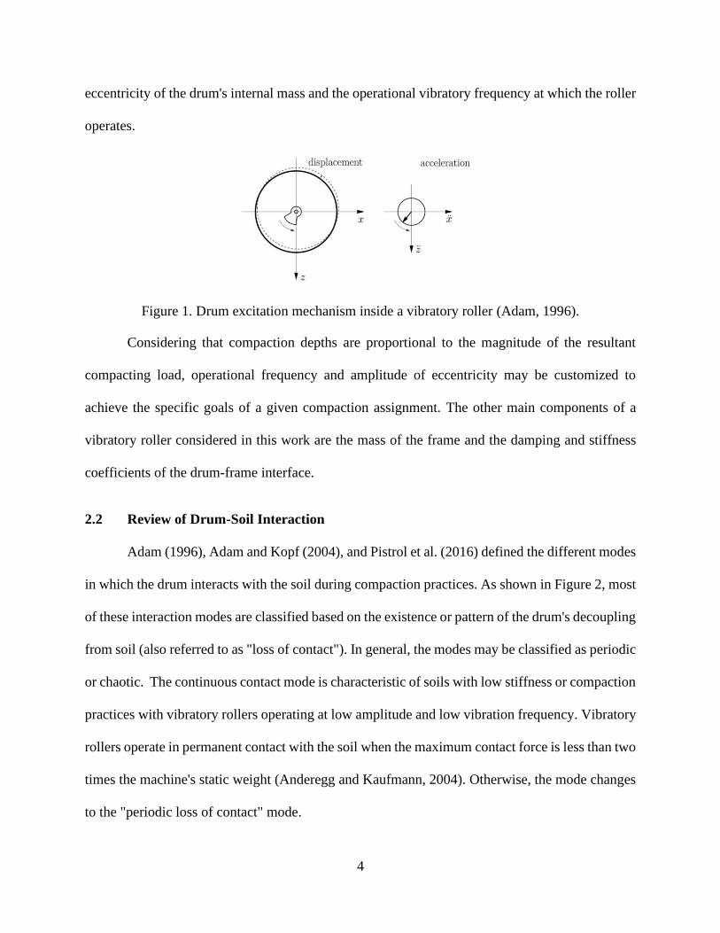
eccentricity of the drum's internal mass and the operational vibratory frequency at which the roller

operates.

Figure 1. Drum excitation mechanism inside a vibratory roller (Adam, 1996).

Considering that compaction depths are proportional to the magnitude of the resultant

compacting load, operational frequency and amplitude of eccentricity may be customized to

achieve the specific goals of a given compaction assignment. The other main components of a

vibratory roller considered in this work are the mass of the frame and the damping and stiffness

coefficients of the drum-frame interface.

2.2 Review of Drum-Soil Interaction

Adam (1996), Adam and Kopf (2004), and Pistrol et al. (2016) defined the different modes

in which the drum interacts with the soil during compaction practices. As shown in Figure 2, most

of these interaction modes are classified based on the existence or pattern of the drum's decoupling

from soil (also referred to as "loss of contact"). In general, the modes may be classified as periodic

or chaotic. The continuous contact mode is characteristic of soils with low stiffness or compaction

practices with vibratory rollers operating at low amplitude and low vibration frequency. Vibratory

rollers operate in permanent contact with the soil when the maximum contact force is less than two

times the machine's static weight (Anderegg and Kaufmann, 2004). Otherwise, the mode changes

to the "periodic loss of contact" mode.

5

The partial uplift interaction mode occurs when the vertical force created by a combination

of eccentric amplitude and drum masses causes a periodic loss of contact at a constant frequency.

Partial uplift is also the target interaction between drum and soil by manufacturers because it is the

most efficient mode of operation and optimizes compaction with vibratory rollers.

Figure 2. Observed modes of vibratory rollers interaction with soil

(Adam, 1996; Adam and Kopf, 2004)

Double jump is a mode of interaction typical of increased soil stiffness when the drum

produces a high jump in every two oscillations and a relatively smaller one in the oscillation in-

between. The energy of the impact when the roller’s drum touches the soil surface after "jumping"

is proportional to the jump's amplitude (or height). Therefore, the highest energy and compaction

are transmitted to the soil in every other oscillation. Although this may provide the required

compaction, it considerably decreases the lifespan of the roller.

A rocking motion occurs when there is a differential settlement due to the compaction

along a roller movement direction. This settlement causes the vibratory roller to be tilted to one

6

side. Rocking motion makes more difficult the operation of the vibratory roller than the previously

mentioned ones.

High heterogeneity in soil mechanical properties and non-ideal roller operating parameters

cause a non-periodic loss of contact, known as chaotic motion. Like the rocking motion, this mode

of operation is not recommended for compaction practices because their associated dynamic

behavior may be unstable and erratic (Anderegg and Kaufmann, 2004).

Among the "continuous contact," "partial uplift," "double jump," "rocking motion," and

"chaotic motion" modes, only the continuous contact, partial uplift, and double jump are

recommended for intelligent compaction (IC) practices from all these modes of drum-soil

interaction.

2.3 Intelligent Compaction Measurement Values

Currently, spot tests with devices such as the nuclear density gauge (NDG), plate load test

(PLT), and the lightweight deflectometer (LWD) are the primary tools for quality management of

compacted geomaterials in the United States and Europe (Nazarian et al., 2020). However, the

spots tested with these devices do not necessarily represent the overall quality nor homogeneity of

the compaction work (Thurner and Sandstrom, 2000). In other words, a shortcoming of spot

testing is that weak areas of a compacted section can be missed.

There is an implicit need for test methods capable of assessing the quality of an entire

compacted section. A correlation between soil stiffness and the motion behavior, as noticed during

an experimental field test with a vibratory roller in 1974 (Pistrol et al., 2016), resulted in the basic

concept of intelligent compaction (IC) through continuous compaction control (CCC) systems. A

CCC system, in general, consists of using the vertical component of the drum acceleration in time

7

and frequency domain to determine the quality of the compacted pavement material (Mooney and

Adam, 2007).

During the following decades, the continuous development of this technology resulted in

different methodologies to estimate the quality and homogeneity of compaction using information

obtained from sensors installed on vibratory rollers. The results of these methodologies are in terms

of Intelligent Compaction Measurement Values (ICMV). Commercially available ICMV with the

vibratory drum parameters needed for their calculation are briefly described in Table 1 (Mooney

et al., 2010). This thesis will only address the Compaction Meter Value (CMV) and Compaction

Control Value (CCV). Both ICMVs are unitless parameters used to estimate mechanical properties

using data obtained during IC operations.

2.3.1 Compaction Meter Value (CMV)

The Compaction Meter Value (CMV) was introduced by the roller manufacturer Dynapac,

in cooperation with Geodynamic, in the late 1970s (Mooney and Adam, 2007). CMV is calculated

from acceleration records in the frequency domain, as illustrated in Figure 3. Also, CMV is defined

as the ratio of the amplitudes of the accelerations at the fundamental frequency (𝐴Ω) and at the

second fundamental frequency (𝐴2Ω) multiplied by a constant c:

𝑪𝑴𝑽 = 𝒄𝑨𝟐𝛀

𝑨𝛀 (1)

The value of constant c is often established as 300 or 100. The plots, results, and discussions

addressed in this document will use a c value of 100 for CMV calculations.

2.3.2 Compaction Control Value (CCV)

The Compaction Control Value (CCV) is the ICMV commercially introduced by roller

manufacturer Sakai. CCV also utilizes the acceleration records in the time domain collected from

8

a sensor attached to the vibratory drum. As shown in Figure 4, the calculation of CCV involves

measuring up to six amplitudes of acceleration at different frequencies (Eq. 2). Acceleration peaks

at subharmonic frequencies are the expected result of a "Double Jump" interaction mode.

Therefore, CCV results are inferred to be more sensitive to all the roller-soil interaction modes.

𝑪𝑪𝑽 = 𝟏𝟎𝟎 × [𝑨𝟎.𝟓𝛀+𝑨𝟏.𝟓𝛀+𝑨𝟐𝛀+𝑨𝟐.𝟓𝛀+𝑨𝟑𝛀

𝑨𝟎.𝟓𝛀+𝑨𝛀] (2)

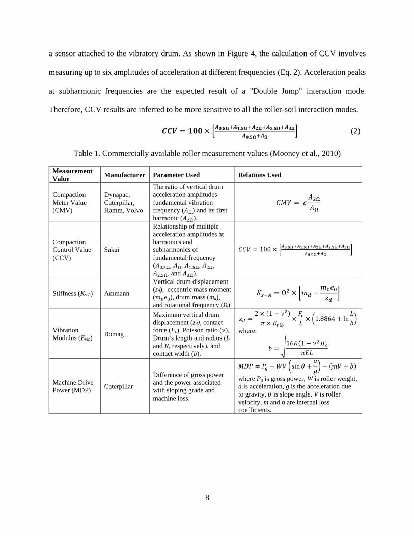
Table 1. Commercially available roller measurement values (Mooney et al., 2010)

Measurement

Value Manufacturer Parameter Used Relations Used

Compaction

Meter Value

(CMV)

Dynapac,

Caterpillar,

Hamm, Volvo

The ratio of vertical drum

acceleration amplitudes

fundamental vibration

frequency (𝐴Ω) and its first

harmonic (𝐴2Ω).

𝐶𝑀𝑉 = 𝑐𝐴2Ω𝐴Ω

Compaction

Control Value

(CCV)

Sakai

Relationship of multiple

acceleration amplitudes at

harmonics and

subharmonics of

fundamental frequency

(𝐴0.5Ω, 𝐴Ω, 𝐴1.5Ω, 𝐴2Ω,

𝐴2.5Ω, and 𝐴3Ω).

𝐶𝐶𝑉 = 100 × [𝐴0.5Ω+𝐴1.5Ω+𝐴2Ω+𝐴2.5Ω+𝐴3Ω

𝐴0.5Ω+𝐴Ω]

Stiffness (Ks-A) Ammann

Vertical drum displacement

(zd), eccentric mass moment

(𝑚0𝑒0), drum mass (md),

and rotational frequency (Ω)

𝐾𝑠−𝐴 = Ω2 × [𝑚𝑑 +

𝑚0𝑒0𝑧𝑑

]

Vibration

Modulus (Evib) Bomag

Maximum vertical drum

displacement (zd), contact

force (Fc), Poisson ratio (𝜈),

Drum’s length and radius (L

and R, respectively), and

contact width (b).

𝑧𝑑 =2 × (1 − 𝜈2)

𝜋 × 𝐸𝑣𝑖𝑏×𝐹𝑐𝐿× (1.8864 + ln

𝐿

𝑏)

where:

𝑏 = √16𝑅(1 − 𝜈2)𝐹𝑐

𝜋𝐸𝐿

Machine Drive

Power (MDP) Caterpillar

Difference of gross power

and the power associated

with sloping grade and

machine loss.

𝑀𝐷𝑃 = 𝑃𝑔 −𝑊𝑉 (sin 𝜃 +𝑎

𝑔) − (𝑚𝑉 + 𝑏)

where Pg is gross power, W is roller weight,

a is acceleration, g is the acceleration due

to gravity, 𝜃 is slope angle, V is roller

velocity, m and b are internal loss

coefficients.

9

Figure 3. (a) Acceleration record in the time domain. (b) Amplitude of acceleration in the

frequency domain (Mooney et al., 2010).

Figure 4. Amplitudes of acceleration in frequency domain used for CCV calculations (Mooney

et al., 2010; Scherocman et al., 2007).

According to (Mooney et al., 2010), both CCV and CMV were determined insensitive to

variations in soil properties when providing values below 10 (unitless result considering c = 300

for CMV calculations). Soft soils are not likely to generate acceleration amplitudes at harmonic

and subharmonic frequencies. Variations in CCV and CMV results are nearly meaningless when

there is a single peak in the amplitude acceleration record in the frequency domain.

10

2.4 Numerical Modeling Techniques of Compacted Geomaterials

The lumped parameter modeling techniques have been used to simulate the interaction of

a vibratory roller with soil during IC operations (Anderegg and Kaufmann, 2004; van Susante and

Mooney, 2008). These techniques model the vertical component of the drum motion during

compaction and the interaction in which the roller transfers a dynamic load to the soil (Neff, 2013).

Lumped parameter models allow simulating the response of soil, considering static masses,

the stiffness and damping coefficients of the drum-frame suspension system, soil stiffness and

damping, and displacements of each of the components. As shown in Figure 5, van Susante and

Mooney (2008) used a three-degree-of-freedom (3DOF) model, which considered the frame,

drum, and soil as three different masses with their corresponding motions. The mass of the frame,

drum, and soil are represented as mf, md, and ms, respectively. Soil stiffness and drum-frame

suspension stiffness are represented with Ks and KD-F, respectively. On the other hand, soil and

drum-frame suspension damping parameters Cs and CD-F that restrain vibratory motions are

essential to simulate the compaction of geomaterials through a spring-damper system.

2.5 Contact Force

Although the contact force cannot be measured directly, this force may be estimated from

the lumped parameter models, knowing the mass of the roller's drum and frame and corresponding

acceleration records. Estimation of contact force has been attempted with available IC information,

neglecting the frame’s mass inertia due to lack of frame acceleration records (Anderegg and

Kaufmann, 2004). Frame's acceleration records improve the estimation of the contact force by

adding the influence of dynamic forces of the frame suspension into the calculations.

The development of a lumped parameter model to simulate IC operations includes

developing an equation to calculate the contact force when the motion records of each model mass

11

element are available. This contact force development is addressed in detail in Chapter 3 of this

document.

Figure 5. 3DOF lumped parameter model (van Susante and Mooney, 2008).

2.6 Summary

A summary of the objectives, scopes, and key findings of relevant literature to IC and CCC

practices is shown in Table 2. Both CMV and CCV can indicate changes in the stiffness of a

geomaterial layer subjected to compaction. The calculation of CMV and CCV requires the

acceleration amplitudes at the fundamental frequency and, at least, a harmonic frequency. The

distribution of drum acceleration amplitude peaks in the frequency domain graphs may

characterize the drum-soil interaction during IC operations. Lumped parameter models have been

proved capable of simulating IC by matching model results with field data collected during IC and

extracting mechanical properties of the geomaterials.

12

Table 2. Literature review of intelligent compaction and lumped parameter models.

Reference Objective and Scope Key Findings

Thurner and

Sandstrom

(2000)

Described the background and principle of

continuous compaction control, compaction

standards, and applications.

Defined CMV as the ratio of the acceleration

amplitude at the fundamental frequency, and at

the first harmonic of the operating frequency.

CCC can increase the efficiency and

homogeneity of the compaction works.

Anderegg

and

Kaufmann

(2004)

Evaluated application potential of feedback

control systems in automatic compaction and

compaction control based on the theory of

nonlinear oscillations.

Vibratory rollers operate in permanent contact

with the soil when the maximum contact force is

less than two times the machine's static weight.

Otherwise, the interaction changes to the

"periodic loss of contact" mode.

(Mooney

and Adam,

2007)

Provided an overview of ICMV history and

theoretical background for measuring soil

properties during IC operations.

ICMVs provide a relative measure of soil

stiffness changes during compaction.

van Susante

and Mooney

(2008)

• The evaluated capability of 3- and 4-degree-

of-freedom lumped parameter models with

linear and nonlinear elements.

• Reproduced vibratory roller behavior

observed experimentally by considering the

loss of contact.

Drum-frame-soil lumped parameter models with

nonlinear soil stiffness can capture soil

parameters from roller vibration data.

Facas et al.

(2010)

Verified a lumped parameter roller/soil model

using field data collected over a range of

excitation frequencies on spatially homogeneous

soil and transversely heterogeneous soil

Rotational motion may occur in both

homogeneous and heterogeneous soil.

Directional independence in roller-measured soil

stiffness can be achieved using vertical vibration

data at the drum center of gravity.

Mooney and

Facas (2013)

• Developed a methodology to extract

composite soil stiffness values from

available vibratory IC rollers.

• Explain the influence of individual

pavement layer properties on the soil

stiffness measured by IC rollers

Forward model results match with available

experimental data.

The calculated soil stiffness increases

proportionally to increments in both maximum

drum displacement and contact force.

Pistrol et al.

(2016)

• Discussed measurement principles and

theoretical background of various ICMVs

• Compared results of large-scale tests using

each of the ICMVs.

"Double Jump" drum-soil interaction mode

results in an additional peak at a subharmonic

frequency on the acceleration record.

Nazarian et

al. (2019)

• Developed procedures to estimate the

mechanical properties of geomaterials using

IC technology.

• Summarized current specifications for

implementing IC technology.

Stiffness-based specifications are almost a real-

time approach for determining field target

values. Unlike spot testing methods, ICMV can

provide quality control on entire compacted

sections.

13

Chapter 3. Development of Lumped Parameter Model

This chapter describes the discrete lumped parameter model representing the roller-soil

interaction developed and utilized in this study to assess the pavement response due to roller

compaction. The discrete lumped parameter model is based on the model proposed by van Susante

and Mooney (2008). The model simulates the mechanical impact and motion generated by the

operation of a vibratory roller during IC operations.

3.1 Model Concept

The developed lumped parameter model intends to simulate the behavior of a vibratory

roller of interest against a specific geomaterial with specific mechanical properties. Although this

model does not consider soil elastic modulus as input and only considers springs and viscous

dampers, elastic modulus can be calculated as discussed at the end of this chapter.

The characteristics of the vibratory roller and properties of soil are modeled with a series

of input parameters. These input parameters influence the total response of the soil (or geomaterial

surface). As shown in Figure 6a, the development of a lumped parameter models the roller’s frame,

vibratory drum, suspension system, and soil as a component able to generate inertial forces and

influence the overall motion. The soil is modeled as a mass connected to a spring-damper

suspension system that simulates the reaction of the soil against the vertical dynamic loading that

the vibratory roller generates.

The mass of the soil is assumed as a fraction of the drum mass. The considered apparent

soil mass has varied from zero (neglecting soil mass) to 62% of the drum mass in similar models

(van Susante and Mooney, 2008), and recent publications used a value of 30% (Mooney and Facas,

2013). The model developed in this thesis is a lumped model that also considers decoupling (or

loss of contact) of the vibratory drum from the geomaterial subject to IC operations, as shown in

14

Figure 6b. The frame and drum are connected through a spring-damper suspension system (KD-F

and CD-F, respectively). The static weight of the frame and drum plus the dynamic forces generated

through vibration are transferred to the soil when the drum and the soil surface are in contact. The

dynamic vertical excitation force (Fecc) as a function of time (t) is calculated from

𝑭𝒆𝒄𝒄 = 𝒎𝟎𝒆𝟎𝛀𝟐 𝐬𝐢𝐧(𝛀𝒕). (3)

The parameters related to this equation are defined in Table 3. As shown in Figure 2, the

consideration of the loss of contact is essential to simulate all the drum-soil interaction modes.

Allowing the loss of contact in a lumped model is necessary for proper simulation of drum-soil

interaction modes during IC operations.

(a) (b)

Figure 6. (a) Vibratory roller lumped model with drum-soil contact. (b) Representation of

lumped model during a loss of contact.

Cs Ks

Frame (mf)

KD-F CD-F

KD-F CD-F

Frame (mf)

Vertical

Excitation

Force (Fecc)

Drum

(md) Drum

(md)

Soil (ms)

Cs Ks

Vertical

Excitation

Force (Fecc)

Soil (ms)

15

Table 3. Description of input parameters in lumped model.

Parameter Variable Units

Drum mass md kg

Frame mass mf kg

Soil mass ms kg

Operating Amplitude A mm

Operating Frequency | Rotational Frequency f | Ω Hz | rad/sec

Eccentric mass moment m0e0 Kg∙m

Drum-frame stiffness KD-F MN/m

Drum-frame damping CD-F kN∙s/m

Soil stiffness Ks MN/m

Soil damping Cs kN∙s/m

Vertical Excitation Force Fecc kN

The lumped model was developed using Simscape (an extension of MATLAB™). This

graphical programming environment enables the simulation of mechanical components and their

response against dynamic loads in the time domain.

As shown in Figure 6, the soil mass, drum mass, frame mass, drum-roller contact

mechanism, suspension systems, and compacted soil mechanical properties were modeled. The

lumped parameter model developed in this document neglects any rotational or transversal motion

that may occur in field operation during IC practices. The model only simulates vertical forces.

Vertical motion records of the soil, drum, and frame are measured through virtual ideal

translational motion sensors in Simscape.

16

Figure 7. Lumped model, as observed in Simscape (Matlab).

3.2 Numerical Model

The development of the multi-degree of freedom lumped parameter described in Section

3.1 is based on the particular motion solutions of the mass components. The ideal translational

motion sensors in the model provide the frame, drum, and soil displacements as zf, zd, and zs,

respectively. The frame is modeled to transfer forces to the drum through the drum-frame

suspension system (KD-F and CD-F). From the frame’s free body diagram shown in Figure 8, a

relationship between the drum-frame suspension system and frame motion can be developed using

−𝑲𝑫−𝑭(𝒛𝒅 – 𝒛𝒇) − 𝑪𝑫−𝑭(�̇�𝒅 − �̇�𝒇) −𝒎𝒇𝒈 = 𝒎𝒇�̈�𝒇 (4)

−𝑲𝑫−𝑭(𝒛𝒅 – 𝒛𝒇) − 𝑪𝑫−𝑭(�̇�𝒅 − �̇�𝒇) = 𝒎𝒇�̈�𝒇 +𝒎𝒇𝒈 (5)

mf

md

ms

KD-F CD-F

Ks Cs

Hard stop

17

Figure 8. Free-body diagram of frame mass.

As shown in Figure 9, the drum transfers frame’s suspension reacting forces in addition to

drum and soil static weights, vertical excitation force (Fecc), and inertial mass to the spring-damper

compacted geomaterial model. Eqs. 6-7 display the summation of vertical forces and solve for the

soil spring-damper reacting force.

𝑲𝒔𝒛𝒔 + 𝑪𝒔�̇�𝒔 +𝑲𝑫−𝑭(𝒛𝒅 – 𝒛𝒇) + 𝑪𝑫−𝑭(�̇�𝒅 − �̇�𝒇) − (𝒎𝒅 +𝒎𝒔)𝒈 + 𝑭𝒆𝒄𝒄 = 𝒎𝒅�̈�𝒅 +𝒎𝒔�̈�𝒔 (6)

𝑲𝒔𝒛𝒔 + 𝑪𝒔�̇�𝒔 = −𝑲𝑫−𝑭(𝒛𝒅 – 𝒛𝒇) − 𝑪𝑫−𝑭(�̇�𝒅 − �̇�𝒇) + (𝒎𝒅 +𝒎𝒔)𝒈 − 𝑭𝒆𝒄𝒄 +𝒎𝒅�̈�𝒅 +𝒎𝒔�̈�𝒔 (7)

Figure 9. Free body diagram of drum attached the soil mass.

18

Drum-frame stiffness and damping coefficients can be replaced by frame mass and

acceleration records by substituting Eq. 5 into Eq. 7. The reacting forces from the soil spring-

damper pair result from adding static weights to inertial masses and subtracting the vertical

excitation force, as shown in Eqs. 8 and 9.

𝑲𝒔𝒛𝒔 + 𝑪𝒔�̇�𝒔 = 𝒎𝒇�̈�𝒇 +𝒎𝒇𝒈+ (𝒎𝒅 +𝒎𝒔)𝒈 − 𝑭𝒆𝒄𝒄 +𝒎𝒅�̈�𝒅 +𝒎𝒔�̈�𝒔 (8)

𝑲𝒔𝒛𝒔 + 𝑪𝒔�̇�𝒔 = 𝐬𝐭𝐚𝐭𝐢𝐜 𝐰𝐞𝐢𝐠𝐡𝐭 − 𝐯𝐞𝐫𝐭𝐢𝐜𝐚𝐥 𝐞𝐱𝐜𝐢𝐭𝐚𝐭𝐢𝐨𝐧 𝐟𝐨𝐫𝐜𝐞 + 𝐢𝐧𝐞𝐫𝐭𝐢𝐚𝐥 𝐦𝐚𝐬𝐬𝐞𝐬 (9)

As shown in Figure 10, the force affecting the soil spring-damper pair is different than in

Figure 9 during a loss of drum-soil contact. During the instant drum decouples from the soil

element, the reacting soil spring-forces are affected only by the soil static weight and inertia, as

shown in Eq. 10.

𝑲𝒔𝒛𝒔 + 𝑪𝒔�̇�𝒔 = 𝒎𝒔𝒈+𝒎𝒔�̈�𝒔 (10)

Figure 10. Forces acting on the spring-damper simulated soil during loss of contact.

The soil mass is modeled as an element attached to the soil spring-damper mechanism in

permanent contact. Contact force (Fc) is the sum of forces exciting motion in the modeled soil

spring-damper mechanism. Soil mass adds to Fc even during loss of drum-soil contact, as shown

in Eq. 11.

𝑭𝒄 = 𝑲𝒔𝒛𝒔 + 𝑪𝒔�̇�𝒔 = {(𝒎𝒇 +𝒎𝒅 +𝒎𝒔)𝒈 − 𝑭𝒆𝒄𝒄 +𝒎𝒇�̈�𝒇 +𝒎𝒅�̈�𝒅 +𝒎𝒔�̈�𝒔

𝒎𝒔𝒈+𝒎𝒔�̈�𝒔 (11) (contact)

(loss of contact)

19

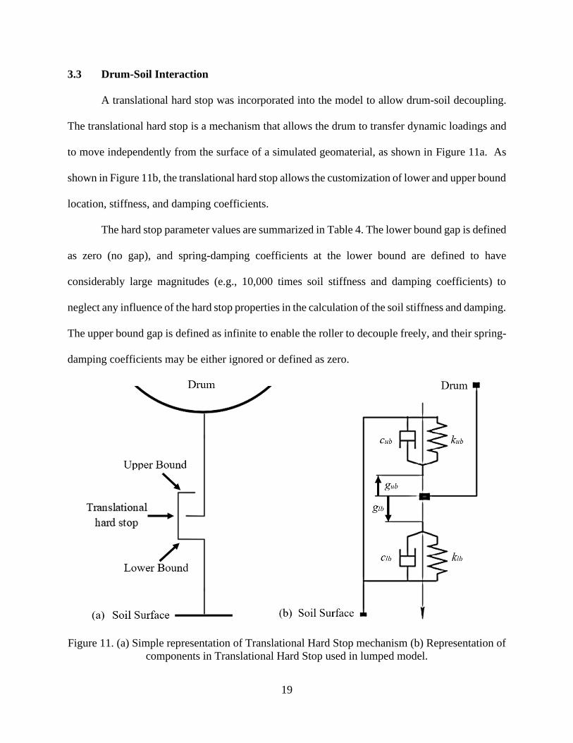
3.3 Drum-Soil Interaction

A translational hard stop was incorporated into the model to allow drum-soil decoupling.

The translational hard stop is a mechanism that allows the drum to transfer dynamic loadings and

to move independently from the surface of a simulated geomaterial, as shown in Figure 11a. As

shown in Figure 11b, the translational hard stop allows the customization of lower and upper bound

location, stiffness, and damping coefficients.

The hard stop parameter values are summarized in Table 4. The lower bound gap is defined

as zero (no gap), and spring-damping coefficients at the lower bound are defined to have

considerably large magnitudes (e.g., 10,000 times soil stiffness and damping coefficients) to

neglect any influence of the hard stop properties in the calculation of the soil stiffness and damping.

The upper bound gap is defined as infinite to enable the roller to decouple freely, and their spring-

damping coefficients may be either ignored or defined as zero.

Figure 11. (a) Simple representation of Translational Hard Stop mechanism (b) Representation of

components in Translational Hard Stop used in lumped model.

20

Table 4. Hard stop assumed parameters for roller-soil interaction simulation.

Parameter Bound Variable Value

Stiffness Coefficient Upper kub 0

Lower klb 10,000 Ks

Damping Coefficient Upper cub 0

Lower clb 10,000 Cs

Gap Upper gub Infinite

Lower glb 0

3.4 Model Behavior

For the continuous contact mode, the displacement of the geomaterial surface is the same

as the roller’s drum displacement, as shown in Figure 12a. Displacements are positive downward

and neglect the displacement due to settlement from the static weight of the roller. The difference

between the drum and soil displacements is calculated and plotted to determine the drum-soil

interaction mode, as shown in Figure 12b.

The drum-soil interaction is characterized as the loss-of-contact mode described in Figure

2 when resultants are greater than zero. Otherwise, the drum-soil interaction mode is continuous

contact. As shown in Figure 1212c, the contact force (Fc) is inverted to signify that a positive

force corresponds to a downward movement. Hysteresis loops help visualize the development of

contact force through periodic displacements. As shown in Figure 12d, an oval-like pattern

represents a continuous contact drum-soil interaction mode.

The Fast-Fourier-Transform (FFT) method can be applied to the motion and contact force-

time histories to obtain the amplitudes in the frequency domain. The determination of the

displacements (Figure 13a) and contact force (Figure 13b) in the frequency domain facilitates

understanding the characteristics of the interaction between the roller and the simulated surface of

the geomaterial.

21

Figure 12. Sample model responses during continuous contact drum-soil interaction mode.

Amplitudes in the frequency domain indicate representative magnitudes of the absolute

difference between the periodic crest (or trough) and its offset (i.e., the center of the signal). For

instance, in Figure 12c, the contact force (Fc) oscillates between 40 and 125 kN, with an estimated

offset of about 82.5 kN. This offset is associated with the static weight of the roller. Thus, the

amplitude of Fc is about 42.5 kN. The magnitude of this amplitude is seen as a peak in the

frequency domain in Figure 13b.

(a) Soil-Drum Displacement (b) Drum Decoupling

(c) Contact Force (d) Force-Displacement Hysteresis Loop

22

Figure 13. Sample model responses during continuous contact drum-soil interaction mode in the

frequency domain.

The magnitudes of the displacement and contact force due to the static weight of the roller

must be added to the amplitudes calculated from the FFT operations to obtain the maximum

displacement and maximum contact force, respectively. Similar to the drum displacement record

in the frequency domain, soil displacement time history can be turned into the frequency domain,

as shown in Figure 13c. Soil displacement in the frequency domain provides valuable information,

especially when there is a loss of drum-soil contact.

During continuous contact interaction mode, the soil and drum displacement amplitudes

are of equal magnitude, as seen in Figure 13a and Figure 13c. The amplitude of drum acceleration

(c) Soil Displacement

(a) Drum Displacement (b) Contact Force

(d) Drum Acceleration

23

in the frequency domain is shown in Figure 13d. The magnitudes of amplitudes of drum

acceleration are essential for the calculation of CMV and CCV.

In each figure, a single peak amplitude corresponding to the roller frequency of operation

is apparent. Both CMV and CCV would provide near-zero results during continuous contact mode

due to the lack of amplitudes at harmonic or subharmonic frequencies. Therefore, the magnitudes

of CMV and CCV are negligible during continuous contact mode.

An example of the soil-drum interaction when partial uplift occurs can be observed in

Figure 14. Partial uplift mode generally occurs on stiffer geomaterials as compared to geomaterials

that produce continuous contact mode with the same roller.

Figure 14. Sample model responses during partial uplift drum-soil interaction mode.

(a) Soil-Drum Displacement

(b) Drum Decoupling

(c) Contact force (d) Force-Displacement Hysteresis Loop

Pattern change

24

The decoupling of the drum from the soil displacements is seen in Figure 14a, indicating

partial uplift. The loss of the drum-soil contact can be observed in Figure 14b as the periodic peaks

in the differences between the roller and soil displacements.

A change in the sinusoidal pattern of the contact force is apparent at the same time the

drum decouples from the soil, as seen in Figure 14c. The change in the slope may be associated

with the drum's impact on the soil. As shown in Figure 14d, the hysteresis loop during the partial

uplift mode displays a truncated oval-like pattern. The partial uplift may also cause the truncated

section of the hysteresis loop (on the negative displacement end).

Figure 15 shows the frequency-domain responses associated with the pavement and roller

operating condition causing partial uplift illustrated in the time-domain responses described in

Figure 14.

The loss of contact between the drum and the geomaterial results in additional amplitude

peaks in harmonic frequencies. As shown in Figure 15a and Figure 15c, the drum and soil

displacement amplitudes differ. This difference is associated with the motion the drum experiences

during the partial uplift. As observed in Figure 15b, contact force amplitude peaks at the

fundamental and harmonic frequencies can be obtained during partial uplift. The additional peaks

at harmonic frequencies, in Figure 15d, are used to calculate CMV and CCV values.

The simulated drum and soil responses under the double jump mode are presented in Figure

16. The loss of drum-soil contact is evident in Figure 16a due to the periodic drum-soil decoupling.

However, the “double jump” impact of the roller can be particularly appreciated in Figure 16b

when two different “jump” heights periodically occur. In addition, a drastic change in the slope of

the contact force occurs concurrently at the moment the drum impacts the soil, as seen in Figure

16c. This change in slope varies depending on the magnitude of the maximum separation between

25

the drum and soil. As shown in Figure 16d, a pair of apparently concentric hysteresis loops seem

to overlap. The magnitude of the maximum contact force is proportional to the maximum drum

displacement.

Figure 15. Sample model responses during partial uplift drum-soil interaction mode.

(c) Soil Displacement

(a) Drum Displacement (b) Contact Force

(d) Drum Acceleration

26

Figure 16. Sample model responses during double jump drum-soil interaction mode.

As shown in Figure 17, multiple amplitude peaks are present in all spectra. The six

amplitude peaks (shown in Figure 4) needed to calculate a CCV can be extracted from the

acceleration spectrum in Figure 17d. As observed in Figure 17b, contact force amplitude peaks at

the fundamental, harmonic and subharmonic frequencies can be obtained during “double jump”

mode. The differences between the soil and drum motion can be observed in the magnitude of the

amplitude peaks in Figure 17a and Figure 17c.

A periodic “multiple jump” interaction mode similar to the one shown in Figure 18 is

observed in very stiff soils. As shown in Figures 18a and 18b, the loss of contact is considerably

longer and more prominent in terms of time and decoupling distance, respectively, than in the

(a) Soil-Drum Displacement

(b) Drum Decoupling

(c) Contact Force

(d) Force-Displacement Hysteresis Loop

Pattern changes

27

previously observed values in Figures 16a and 16b. Figure 18c suggests that multiple periodic

contact force patterns occur simultaneously, resulting in overlapped hysteresis loops, as shown in

Figure 18d.

Figure 17. Sample model responses during double jump drum-soil interaction mode.

(a) Drum Displacement (b) Contact Force

(c) Soil Displacement (d) Drum Acceleration

28

Figure 18. Sample model responses during “multiple” jump drum-soil interaction mode.

The motion and contact force records in the frequency domain display amplitude peaks at

the harmonic and at multiple subharmonic frequencies, as shown in Figure 19. A significant

difference between the soil and drum motion amplitudes can be observed in Figure 19a and Figure

19b. Such difference is attributed to a considerable amount of time the drum remains separated

from the soil per oscillation. For example, Figure 19b and Figure 19d results provide amplitude

peaks at 15, 22.5, 30, 37.5, 45, and 60 Hz when Figure 17b and Figure 17d only show amplitude

peaks at 15, 30, 45, and 60 Hz. In addition, spectra displaying multiple harmonic and subharmonic

frequencies, as seen in Figure 19d may provide drum acceleration amplitudes at frequencies not

considered by the CCV or the CMV calculations.

(a) Soil-Drum Displacement (b) Drum Decoupling

(c) Contact Force (d) Force-Displacement

Hysteresis Loop

29

Figure 19. Model behavior example with “multiple” jump drum-soil interaction mode.

The impact of neglecting those additional acceleration amplitude values at subharmonic

frequencies is unknown with the currently available ICMVs. Therefore, CMV and CCV results on

geomaterials stiff enough to show “multiple jump” behavior during IC operations might not

represent the soil stiffness as those extracted from IC operations with continuous contact, partial

uplift, or double jump interaction modes. Drum acceleration amplitude records in the frequency

domain for different drum-soil interaction modes can be observed in Figure 20.

In summary, during continuous, a single acceleration amplitude peaks at the fundamental

frequency of operation, as seen in Figure 20a. During partial uplift mode, there are amplitude peaks

at harmonic frequencies (Figure 20b). Double jump mode generates amplitudes at multiples of half

(a) Drum Displacement

(b) Contact Force

(c) Soil displacement

(d) Drum Acceleration

30

the fundamental frequency (Figure 20c). Moreover, amplitude peaks at additional subharmonic

frequencies are present during multiple jump mode, as observed in Figure 20d.

Figure 20. Sample of drum acceleration in the frequency domain for different drum-soil

interaction modes.

The following section departs from the numerical model displayed in current sections and

proceeds to describe the estimation of the geomaterial mechanical properties, in terms of soil

stiffness (Ks, MN/m), and Elastic Modulus (E, MPa)

(a) Continuous Contact (b) Partial Uplift

(d) Double Jump (d) Multiple Jumps

31

3.5 Extraction of Mechanical Properties

The mechanical properties calculation involves principally using the information related to

the contact force and displacements generated during IC operations. Instrumenting soil to measure

its acceleration during compaction is not feasible. Available drum acceleration records may be

subjected to two different procedures to calculate soil stiffness: Secant Method and FFT method.

3.5.1 Secant Method

The secant method provides a result used by Bomag or Amman/Case to estimate soil

stiffness (Mooney and Facas, 2013). As shown in Figure 21, this method calculates the slope of a

line that starts at the center of the hysteresis loop and ends at the point of maximum drum

displacement. The center of the hysteresis loop is assumed to be where the vibratory displacement

is zero and the contact force equal to the static weight of the vibratory roller. The soil stiffness, 𝑘𝑠,

is estimated from (Kenneally et al., 2015),

𝒌𝒔 =𝑭𝒄 (@𝑴𝑨𝑿 𝒛𝒅)−𝑭𝒄 (𝑺𝑻𝑨𝑻𝑰𝑪)

𝒛𝒅 (𝑴𝑨𝑿)−𝒛𝒅 (𝑺𝑻𝑨𝑻𝑰𝑪) (12)

defined as the ratio of the difference of contact force at maximum displacement and static weight

to the difference of their respective drum displacements.

Figure 21. Conceptual representation of Secant Stiffness during (a) continuous contact and (b)

loss of drum-soil contact (Mooney et al., 2010).

32

The four hysteresis loops and the lines from which the secant stiffness values are estimated

for the samples discussed in Section 3.4 can be observed in Figure 22. Table 5 summarizes the

results of secant stiffness in the examples shown in Section 3.4 and provides percent error.

Figure 22. Contact Force – Displacement Hysteresis Loops Samples generated by the same roller

at different soil stiffness values.

Table 5. Comparison of secant stiffness results vs model stiffness values.

Model Stiffness

(MN/m)

Calculated Secant

Ks (MN/M)

% Error

40 40 0.8

100 101 0.7

125 125 0.2

400 396 0.9

(a) Continuous Contact (b) Partial Uplift

(c) Double Jump (d) Multiple Jump

33

3.5.2 FFT Method

The Fast Fourier transform (FFT) consists of an algorithm that can transform a time-

domain signal into a representation of signal amplitude in the frequency domain (i.e., a transition

from Figure 12a to Figure 13a).

During IC, the roller operates at a known rotational frequency Ω (aka fundamental

frequency). Therefore, the motion and contact force spectrums are expected to show maximum

values at Ω. Stiffness, in general, is defined as the amount of force required to generate a unit

displacement. The calculation of FFT soil stiffness Ks consists of the absolute value of the result

of dividing the amplitude of contact force (Fc) by the amplitude of drum displacement (zd), both

in complex numbers at Ω. Therefore, the “FFT” soil stiffness, 𝑘𝑠, is calculated from

𝒌𝒔 = |𝑭𝑭𝑻(𝑭𝒄 ) (@𝛀)

𝑭𝑭𝑻(𝒛𝒅 ) (@𝛀) | (13)

where 𝐹𝐹𝑇(𝐹𝑐 ) (@Ω) is the amplitude of contact force in complex numbers at the Ω (as seen in

Figure 24), and 𝐹𝐹𝑇(𝑧𝑑 ) (@Ω) is the amplitude of the drum displacement in complex cumbers at

Ω (as shown in Figure 25).

For example, the amplitude of 𝐹𝑐 spectrum at Ω is 42 kN (Figure 23a) and the amplitude

of 𝑧𝑑 spectrum at Ω is 0.89 mm (Figure 23b) during a continuous contact drum-soil interaction

mode with a simulated geomaterial stiffness of 40 MN/m. Therefore, “FFT” soil stiffness 𝒌𝒔 results

in 47 MN/m with a resultant relative error is 18%.

The magnitude of Fc(@Ω) varies depending on the simulated geomaterial stiffness and the

drum-soil interaction mode, as shown in Figure 24a-d. The magnitude of 𝐹𝑐 (@Ω) seems to increase

proportionally to the simulated geomaterial stiffness value during continuous contact, partial uplift,

and double jump modes, as seen in Figure 24a-c. Contact force amplitudes at subharmonic

34

Figure 23. Contact force and drum displacement amplitudes during continuous contact mode.

Figure 24. Contact force spectrum for different drum-soil interaction modes.

(a) Continuous Contact (b) Partial Uplift

(c) Double Jump (d) Multiple Jump

𝑭𝒄 (@𝛀)

𝑭𝒄 (@𝛀) = 42 𝑘𝑁

𝒛𝒅 (@𝛀) = 0.89 𝑚𝑚

𝑭𝒄 (@𝛀)

𝑭𝒄 (@𝛀)

𝑭𝒄 (@𝛀)

(a) Contact Force (b) Drum Displacement

35

frequencies resulted in higher values than at fundamental during multiple jump mode, as observed

in Figure 24d.

Figure 25 shows the drum displacement spectrum for continuous contact, partial uplift,

double jump, and multiple jump modes. Figure 25a shows the smallest drum displacement

amplitude among all the displayed samples, and it also increases during the partial uplift mode, a

shown in Figure 25b. The increments in displacement magnitude continue during double jump

mode, as shown in Figure 25c. Finally, the multiple jump drum-soil interaction mode leads to a

reduced displacement amplitude at the fundamental frequency (30 Hz) and higher amplitudes at

other subharmonic frequencies, as seen in Figure 25d.

Figure 25. Drum displacement spectrum for different drum-soil interaction modes

(a) Continuous Contact

(b) Partial Uplift

(c) Double Jump (d) Multiple Jump

𝒛𝒅 (@𝛀)

𝒛𝒅 (@𝛀)

𝒛𝒅 (@𝛀)

𝒛𝒅 (@𝛀)

36

A summary of the soil stiffness values obtained with the FFT method from the four

examples discussed in Section 3.4 is listed in Table 6. The calculated FFT soil stiffness values

differ more from the model stiffness values than the results obtained from the secant method. The

error was above 17% in three out of the four examples. A percent error of 1% was obtained from

the examples with a model stiffness of 100 MN/m.

Table 6. Comparison of FFT stiffness results vs. model stiffness values.

Model Stiffness

(MN/m)

Calculated

“FFT” Ks (MN/m) % Error

40 47 18

100 101 1

125 100 20

400 55 86

During IC practices, where only the drum acceleration data is collected, a method named

Omega Arithmetic is applied to transform the drum acceleration data into drum displacement time

records. However, drum displacement records differ from soil displacement records drum-soil

interaction modes involving loss of contact. The variation between calculated “FFT” and input Ks

is expected to be associated with the different motions the soil and drum experience during the

loss of contact.

As observed in Figure 26, the calculated “FFT” Ks using the soil displacements (obtained

from simulation) provide results closer to the input soil stiffness than those obtained using drum

displacement records. Although calculating “FFT” Ks with soil displacements records provides

results proportional to the input Ks, this is not practical unless the roller can measure soil surface

displacement during IC operations.

37

Figure 26. “FFT” Ks using drum and soil displacement records vs input Ks.

Once stiffness has been calculated by either secant or FFT method, it is of interest to

estimate the modulus of such geomaterial. Therefore, the following section addresses modulus

estimation considering the roller variables and resultant motion during compaction.

3.6 Estimation of Modulus

Lundberg (1939) introduced the following theoretical relationship between the soil

stiffness, ks, and soil modulus, E, for a drum resting on a homogeneous, isotropic elastic half-

space:

𝒌𝒔 =𝑬𝑳𝝅

𝟐(𝟏−𝝂𝟐)

(

𝟏.𝟖𝟖𝟔𝟒+𝐥𝐧

𝑳

√𝟏𝟔𝑹(𝟏−𝝂𝟐)𝑭𝒄

𝝅𝑬𝑳 )

(14)

0

50

100

150

200

250

300

350

400

0 50 100 150 200 250 300 350 400

"FF

T"

Ks

(MN

/m)

Input soil stiffness, Ks (MN/m)

Soil disp. records

Drum disp. records

38

where L and R are the length and radius of the drum, respectively, and is the soil Poisson ratio

(a value of 0.3 was considered in this study). Lundberg’s equation can be used to convert soil

stiffness values and drum motion responses into modulus.

Pavement designs and their geomaterial specifications are often modulus-based. Therefore,

the extraction of modulus from calculated stiffness values enables the comparison of the results of

the developed model with available standards.

39

Chapter 4. Sensitivity Analysis, Results, and Discussion.

This chapter aims to evaluate the impacts of the model variables in the estimation of CMV

and CCV. This evaluation consists of a set of simulations of a specific vibratory roller operating

on a geomaterial, in which a single roller or geomaterial property variable is modified at a time.

Motion response, CMV, and CCV values are collected and analyzed from each simulation.

4.1. OAT Sensitivity Analysis Methodology

The sensitivity study developed in this chapter is based on the one-at-a-time (OAT)

method. It consists of evaluating the results from changing the value of one input variable at a

time. This study considers a standard vibratory roller as the reference roller. Table 7 provides a

listing of the roller variables and their nominal values that are considered in the sensitivity study.

Table 7. Roller variable values for Sakai SV 510D

Sakai SV 510 D

Drum mass 4,466 kg

Frame mass 2,534 kg

Soil mass 1,340 kg

Drum/Frame stiffness 1.27 MN/m

Drum/Frame damping 3.8 kN∙s/m

Operating frequency 30 Hz

Mass moment (m0e0) 4.21 kg∙m

The roller-dependent parameters varied based on the information collected from over 30

commercially available rollers manufactured by Amman, Bomag, Case, CAT, Dynapac, Ingersoll

Rand, Sakai, and Volvo, as summarized in Table 8.

40

Table 8. Parameter value ranges in commercially available vibratory rollers.

Parameter Minimum Maximum

Drum mass, kg 1,600 13,450

Frame mass, kg 1,650 5,450

Operation frequency, Hz 20 60

Amplitude, mm 0.3 2.3

Drum-Frame Stiffness, MN/m 1 6

Drum-Frame Damping kN∙s/m 2 12

Drum width, m 1.2 2.2

Drum diameter, m 0.7 1.6

The calculation of CMV, CCV, Ks, and modulus followed the procedure in Chapter 3.

Development of Lumped Parameter Model. Even though the drum width and diameter are not

input values in the lumped model; they are exclusively used in this study for the estimation of soil

modulus through the Lundberg equation (Eq. 14).

The sensitivity analysis contemplates sets of simulations of 200 cases in which a soil or

roller parameter is uniformly distributed within the range shown in Table 8 while keeping constant

the rest of the reference roller parameters, Ks, and Cs. Each set of simulations was repeated at five

different Ks values of 5 MN/m, 50 MN/m, 100 MN/m, 150 MN/m, and 200 MN/m to evaluate the

impact of soil stiffness in CMV and CCV at different drum-soil interaction modes, except for the

set of simulations that only varies input soil stiffness. The value of Cs (kN∙s/m) was calculated for

every Ks value using

𝑪𝒔 ≈ 𝟐𝟕 ∙ √𝑲𝒔 (15)

where Cs is in kN∙s/m and Ks in MN/m. This Ks to Cs relation was established based on the

results of a best-fit analysis with experimental data performed by van Susante and Mooney (2008).

41

The sensitivity study was organized in the following order. First, the soil stiffness was

varied to evaluate the pattern of CMV, CCV, and modulus while maintaining the reference roller

parameters constant. The value of Ks is varied from 5 to 400 MN/m to identify relationships

between the different drum-soil interaction modes and both CMV and CCV.

In the second study, Cs was uniformly varied in a range of 50% – 150 % of the result from

Eq. 15 to evaluate the impact of fluctuation of soil damping in the motion response for the five

selected soil stiffness, Ks, values (5, 50, 100, 150, and 200 MN/m). Third, the impacts of the

fluctuations of the frame mass, drum mass, and soil mass were evaluated. Fourth, the influence of

variations in the frame-drum suspension constants (KD-F and CD-F) were evaluated. Finally, the

impact of fluctuations in the operational frequency (f ) and amplitude were evaluated. The reference

roller parameters will be marked with a red bar in the following figures.

4.2 Geomaterial Mechanical Properties

4.2.1 Soil Stiffness

The variations of CMV, CCV, and modulus as a function of input soil stiffness are shown

in Figure 27. Moduli obtained from Eq. 14 exhibit a linear proportionality to modeled soil stiffness.

On the other hand, CMV and CCV are insensitive to changes in soil stiffness for values lower than

80 MN/m. From stiffness values of 80 MN/m to approximately 125 MN/m, an approximate linear

relationship between CMV or CCV and soil stiffness is observed. A change of slope for CMV or

CCV with soil stiffness is observed past a stiffness of 125 MN/m . The slope of the CCV trends

toward a proportional increase with the soil stiffness until 400 MN/m.

On the other hand, CMV becomes inversely proportional to the soil stiffness in the range

of 125-180 MN/m. Also, after a soil stiffness values greater than 180 MN/m, the CMV slope turns

42

back positive, as seen in Figure 27. The results indicate a complex dependency of CMV and CCV

to Ks; therefore, further understanding of the amplitudes in the acceleration spectrum is required.

The drum acceleration amplitudes used for CCV and CMV calculations are plotted

individually against Ks in Figure 28. The amplitude at the fundamental frequency (A2) displays the

highest values, increasing proportionally to the soil stiffness value until approximately a Ks of 120

MN/m; after which it starts decreasing slowly until an apparent “stable” value at a magnitude of

approximately 34 m/s2 is reached.

Figure 27. ICMVs (unitless) vs. modeled soil stiffness (MN/m)

43

Figure 28. Drum acceleration amplitudes vs. soil stiffness.

The magnitudes of A4 and A6 start increasing after a Ks of approximately 86 MN/m,

signifying the threshold of the continuous contact interaction mode and the start of partial uplift

mode. The magnitude of A4 increases within a relatively short range of Ks (86–122 MN/m).

On the other hand, A6 increases within a shorter range (86-100 MN/m) and remains

constant until 122 MN/m. This stiffness value is also the initial Ks from which the magnitudes of

A1, A3, and A5 increase, indicating the start of the double jump drum-soil interaction mode. A4

decreases from a Ks of 122 MN/m to approximately 180 MN/m indicating the complete range in

which the drum-soil interaction mode is in double jump. The interaction mode for Ks greater than

180 MN/m is considered a multiple jump mode. When overlapping the drum-soil interaction mode

thresholds in Figure 27, the interaction mode thresholds determined by analyzing the acceleration

amplitudes match the slope changes for both CMV and CCV, as shown in Figure 29.

44

Figure 29. Drum-soil interaction modes on a CMV + CCV vs. modeled soil stiffness plot.

These results indicate potential proportionality between CCV and Ks during partial uplift,

double jump, and multiple jump drum soil interaction modes for the reference roller. CMV exhibits

proportionality with Ks during partial uplift and multiple jump interaction modes. An inversely

proportional trend between CMV and Ks during double jump mode (122-180 MN/m) is observed.

4.2.2 Soil Damping

The reference soil damping coefficient (Cs) values were calculated through Eq. 15 for five

Ks values (5, 50, 100, 150, and 200 MN/m). Then 200 simulations varying Cs within a range of

50% to 150% of its reference value were performed for each Ks. The results from all cases were

normalized with the corresponding values determined with the reference Cs

As observed in Figure 30, the sets corresponding to Ks = 5 MN/m and Ks = 50 MN/m did

not show a change in magnitude, indicating that the fluctuation of soil damping coefficient did not

Co

nti

nu

ou

s co

nta

ct

Par

tial

upli

ft

Double

Jum

p

Multiple Jump

45

modify the continuous contact interaction mode due to their near-zero values. On the other hand,

for Ks equal to 100, 150, and 200 MN/m, the CMV changed without apparent trends.

Figure 30. Impact of soil damping coefficient in CMV for five different soil stiffness values.

Figure 31 displays the variations of CCV with normalized Cs for five different Ks values.

No fluctuation was observed for the two lowest Ks values. For Ks equal 100 MN/m, CCV results

varied almost linearly from 8 to 21. In the case of Ks equal to 150 MN/m, the values are relatively

stable for Cs / Cs-ref. of 0.5 to 1.2. Finally, for Ks equal to 200 MN/m, CCV only varied between 55

and 63 within all Cs values considered. There are differences between the behavior of CMV and

CCV when the soil damping constant varies. ICMV results fluctuations are more predictable for

CCV than they are for CMV in most cases.

0

2

4

6

8

10

12

14

16

18

20

22

24

0.5 0.6 0.7 0.8 0.9 1.0 1.1 1.2 1.3 1.4 1.5

CM

V

Cs /Cs-ref.

ks = 5 MN/m

ks = 50 MN/m

ks = 100 MN/m

ks = 150 MN/m

ks = 200 MN/m

46

Figure 31. Impact of soil damping coefficient in CCV for five different soil stiffness values.

4.3 Static Weight

This section evaluates the impact of the static masses one at a time. Each set of simulations

consisted of 200 cases in which the masses were perturbed within the range defined in Table 8.

4.3.1 Frame Mass

As shown in Figure 32, CMV does not change for the two lowest Ks values. For Ks of 100,

150, and 200 MN/m the behaviors differ from one to another within the range of frame masses

considered. CMV stabilizes after frame mass with at least 4,500 kg for the five simulated Ks values.

As seen in Figure 33, for Ks of 200 MN/m, CCV does not fluctuate much for frame masses

of 1,650 kg to 3,500 kg. Then, an abrupt decrease in CCV occurs between frame masses of 3,500

kg and 3,800 kg. For Ks of 150 MN/m, similar behavior is observed, in which CCV remains

constant after an abrupt decrement. CCV values are inversely proportional to the frame mass for a

Ks of 100 MN/m. For Ks of 5 MN/m and 50 MN/m, CCV values are rather small and constant.

0

5

10

15

20

25

30

35

40

45

50

55

60

65

70

0.5 0.6 0.7 0.8 0.9 1.0 1.1 1.2 1.3 1.4 1.5

CC

V

Cs /Cs-ref.

ks = 5 MN/m

ks = 50 MN/m

ks = 100 MN/m

ks = 150 MN/m

ks = 200 MN/m

47

Figure 32. Impact of frame mass in CMV results for five Ks values.

Figure 33. Impact of frame mass in CCV results for five Ks values.

0

5

10

15

20

25

1,500 2,000 2,500 3,000 3,500 4,000 4,500 5,000

CM

V

Frame mass (kg)

ks = 5 MN/m

ks = 50 MN/m

ks = 100 MN/m

ks = 150 MN/m

ks = 200 MN/m

0

10

20

30

40

50

60

70

1,500 2,000 2,500 3,000 3,500 4,000 4,500 5,000 5,500

CC

V

Frame mass (kg)

ks = 5 MN/m

ks = 50 MN/m

ks = 100 MN/m

ks = 150 MN/m

ks = 200 MN/m

48

4.3.2 Drum Mass

As observed in Figure 34, there are no apparent changes in CMV for the two lowest Ks

values when the drum mass varies within the range established in Table 8. For all the other

simulated Ks values (100, 150, and 200 MN/m), the CMV shows a “zigzag” behavior between the

CCV and drum mass. In those cases, CMV values tend to zero as the drum mass exceeds a certain

value. Thus, a roller with a given drum mass will not reflect CMV values unless the soil achieves

a specific stiffness through compaction.

On the other hand, CCV exhibits an inversely proportional pattern with the drum mass for

a given soil stiffness, as seen in Figure 35. This is the only case in which Ks = 50 MN/m simulation

CMV and CCV results deviate from near-zero values. This indicates that rollers with lighter drums

are more sensitive to changes in low Ks values than those with heavier drums and vice versa. The

drum mass value in which each simulation reaches a near-zero value coincides with the values

observed in Figure 34. Both Figure 34 and Figure 35 indicate the importance of the drum mass

and its relevance in calculating CCV values and coinciding in the drum mass limit in which the

system will become insensitive for a given soil stiffness value.

4.3.3 Assumed Soil Mass

The mass of soil has been modeled as a fraction of the mass of the drum. In this set of

simulations, the soil mass varied from 0 to 60% of the mass of the drum, while keeping all the

other parameters constant. The reference assumed soil mass during all simulations performed was

0.3 (30%) times the mass of the drum. As observed in Figure 36, the variation in CMV with the

soil mass is dependent on Ks (except for 5 and 50 MN/m that generate operations in continuous

contact interaction mode).

49

Figure 34. Impact of drum mass in CMV results for five Ks values.

Figure 35. Impact of drum mass in CCV results for five Ks values.

0

5

10

15

20

25

1,000 2,500 4,000 5,500 7,000 8,500 10,000 11,500 13,000

CM

V

Drum mass (kg)

ks = 5 MN/m

ks = 50 MN/m

ks = 100 MN/m

ks = 150 MN/m

ks = 200 MN/m

0

10

20

30

40

50

60

70

80

90

1,000 2,500 4,000 5,500 7,000 8,500 10,000 11,500 13,000

CC

V

Drum mass (kg)

ks = 5 MN/m

ks = 50 MN/m

ks = 100 MN/m

ks = 150 MN/m

ks = 200 MN/m

50

Figure 36. Impact of soil mass in CMV results for five Ks values.

Figure 37. Impact of soil mass in CCV results for five Ks values.

0

5

10

15

20

25

0.0 0.1 0.2 0.3 0.4 0.5 0.6

CM

V

Ms/Md

ks = 5 MN/m

ks = 50 MN/m

ks = 100 MN/m

ks = 150 MN/m

ks = 200 MN/m

0

10

20

30

40

50

60

70

80

90

0.0 0.1 0.2 0.3 0.4 0.5 0.6

CC

V

Ms/Md

ks = 5 MN/m

ks = 50 MN/m

ks = 100 MN/m

ks = 150 MN/m

ks = 200 MN/m

51

On the other hand, CCV varies in an inversely proportional manner with the soil mass for

Ks values of 100, 150, and 200 MN/m, as observed in Figure 37. Again, the soft soils are not

impacted by the variation in the soil mass.

4.4 Frame-Drum Suspension System

4.4.1 Frame-Drum Stiffness (KD-F)

As observed in Figure 38, CMV values are mostly constant for KD-F values less than 2.5

MN/m. CMV maintains a constant value for Ks of 5 MN/m, 50 MN/m, and 100 MN/m,

independent of KD-F.

Figure 38. Impact of drum-frame suspension stiffness in CMV results for five Ks values.

The variations in CCV with KD-F in Figure 39 are rather constant up to a KD-F of about 4.5

MN/m. The impact of KD-F fluctuations seems minimal for CCV results in most cases. However,

a drastic change in CMV and CCV for Ks of 150 MN/m and 200 MN/m was observed at KD-F

between 5.1MN/m and 5.4 MN/m

0

5

10

15

20

25

1.0 1.5 2.0 2.5 3.0 3.5 4.0 4.5 5.0 5.5 6.0

CM

V

Drum-Frame Stiffness, MN/m

ks = 5 MN/m

ks = 50 MN/m

ks = 100 MN/m

ks = 150 MN/m

ks = 200 MN/m

52

Figure 39. Impact of drum-frame suspension stiffness in CCV results for five Ks values.

4.4.2 Frame-Drum Damping (CD-F)

As observed in Figure 40, CMV remains relatively constant as CD-F varies for all Ks values.

Some fluctuations are observed at the higher CD-F values. Similar trends are observed in Figure 41,

for CCV. In general, both sets of simulations reflect the neglectable influence of CD-F in CMV and

CCV results within the 2-12 kN∙s/m range.

0

10

20

30

40

50

60

70

1.0 1.5 2.0 2.5 3.0 3.5 4.0 4.5 5.0 5.5 6.0

CC

V

Drum-Frame Stiffness, MN/m

ks = 5 MN/m

ks = 50 MN/m

ks = 100 MN/m

ks = 150 MN/m

ks = 200 MN/m

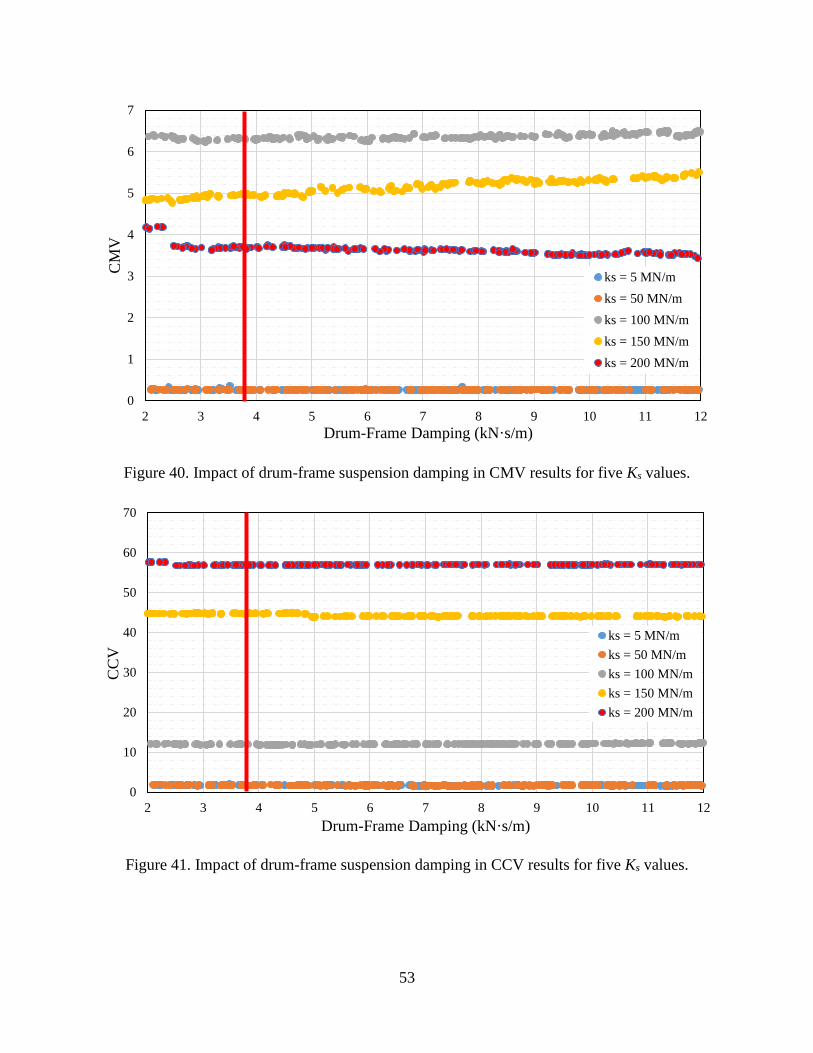
53

Figure 40. Impact of drum-frame suspension damping in CMV results for five Ks values.

Figure 41. Impact of drum-frame suspension damping in CCV results for five Ks values.

0

1

2

3

4

5

6

7

2 3 4 5 6 7 8 9 10 11 12

CM

V

Drum-Frame Damping (kN·s/m)

ks = 5 MN/m

ks = 50 MN/m

ks = 100 MN/m

ks = 150 MN/m

ks = 200 MN/m

0

10

20

30

40

50

60

70

2 3 4 5 6 7 8 9 10 11 12

CC

V

Drum-Frame Damping (kN·s/m)

ks = 5 MN/m

ks = 50 MN/m

ks = 100 MN/m

ks = 150 MN/m

ks = 200 MN/m

54

4.5 Eccentric Mass System

4.5.1 Operating Frequency

As observed in Figure 42, the variations in CMV with the operating frequency (f) remained

reasonably constant until an upper f of 44 and 47 Hz for Ks of 5 MN/m and 50 MN/m, respectively.

Above those frequencies, CMV gradually increased with f. On the other hand, for Ks of 100 MN/m,

150 MN/m, and 200 MN/m, CMV decreases inversely proportional to f during the approximately

20-35 Hz range until reaching steady values.

CCV results are sensitive to variations in f, as observed in Figure 43. For Ks of up to 100

KN/m, the trends of the variations in CCV with f are similar to the variations of CMV with f. For

Ks of 150 MN/m and 200 MN/m, CCV values are constant with large dispersion up to f of 40 Hz

to 45 Hz.

Figure 42. Impact of rotating frequency ( f ) in CMV results for five Ks values.

0

10

20

30

40

50

60

70

20 25 30 35 40 45 50 55 60

CM

V

Rotational Frequency, Hz

ks = 5 MN/m

ks = 50 MN/m

ks = 100 MN/m

ks = 150 MN/m

ks = 200 MN/m

55

Figure 43. Impact of operational frequency ( f ) in CCV results for five Ks values.

4.5.2 Amplitude

The reference amplitude is considered as the resultant of dividing m0e0 (eccentric mass

moment) by md (drum mass), using the values provided in Table 7. In practice, the amplitude is

inversely proportional to the operating frequency ( f ) in compaction operations; therefore,

operations are normally classified as “low-amplitude” (low A at high f ) and “high-amplitude”

(high A at low f ).

As observed in Figure 44, CMV fluctuates significantly with the amplitude, except for the

soils with Ks of less than 50 MN/m. The CCV values are also variable in a similar manner as the

CMV values, as shown in Figure 45. There are two ranges of amplitude (0.5-0.75 mm and 0.8-

1.15 mm) in which CCV slightly varies in amplitude.

0

10

20

30

40

50

60

70

80

90

100

20 25 30 35 40 45 50 55 60

CC

V

Rotational Frequency, Hz

ks = 5 MN/m

ks = 50 MN/m

ks = 100 MN/m

ks = 150 MN/m

ks = 200 MN/m

56

Figure 44. Impact of operational Amplitude (A) in CMV results for five Ks values.

Figure 45. Impact of operational Amplitude (A) in CCV results for five Ks values.

0

5

10

15

20

25

0.3 0.5 0.7 0.9 1.1 1.3 1.5 1.7 1.9 2.1 2.3

CM

V

Amplitude, mm

ks = 5 MN/m

ks = 50 MN/m

ks = 100 MN/m

ks = 150 MN/m

ks = 200 MN/m

0

10

20

30

40

50

60

70

80

0.3 0.5 0.7 0.9 1.1 1.3 1.5 1.7 1.9 2.1 2.3

CC

V

Amplitude, mm

ks = 5 MN/m

ks = 50 MN/m

ks = 100 MN/m

ks = 150 MN/m

ks = 200 MN/m

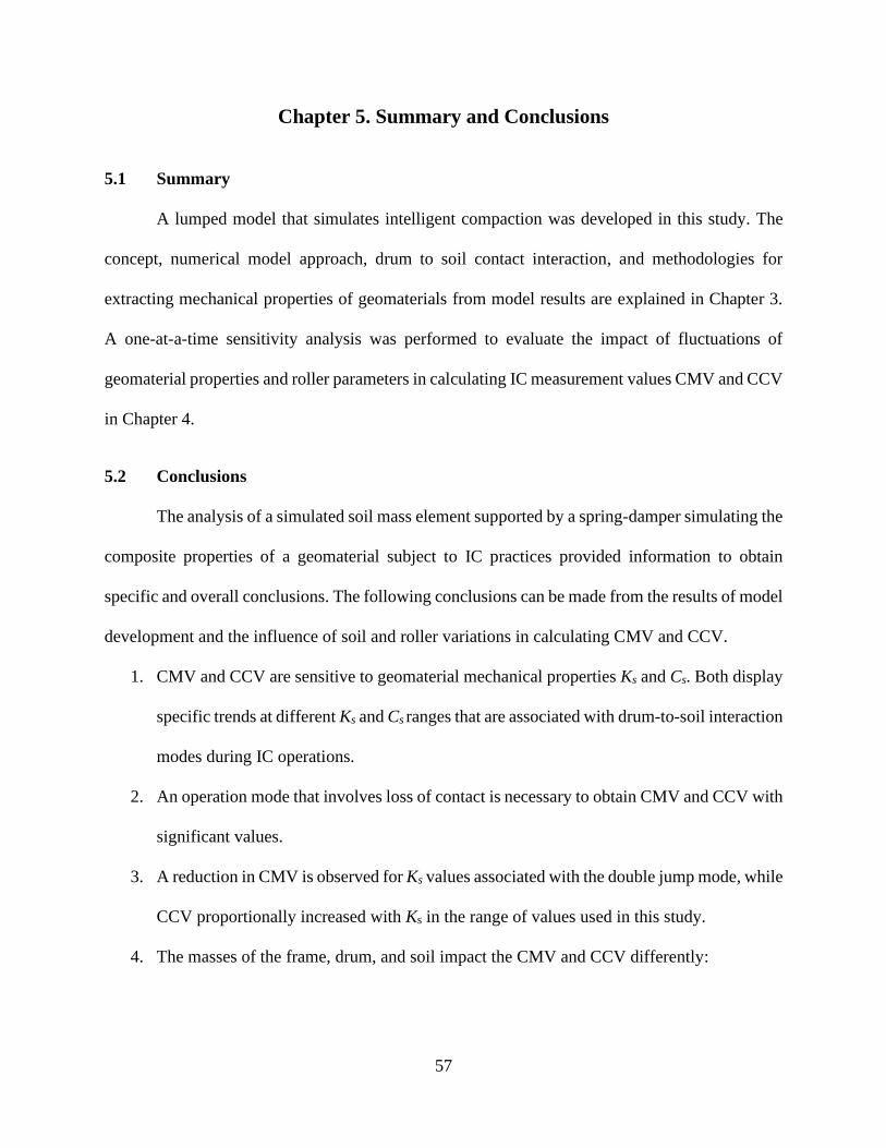
57

Chapter 5. Summary and Conclusions

5.1 Summary

A lumped model that simulates intelligent compaction was developed in this study. The

concept, numerical model approach, drum to soil contact interaction, and methodologies for

extracting mechanical properties of geomaterials from model results are explained in Chapter 3.

A one-at-a-time sensitivity analysis was performed to evaluate the impact of fluctuations of

geomaterial properties and roller parameters in calculating IC measurement values CMV and CCV

in Chapter 4.

5.2 Conclusions

The analysis of a simulated soil mass element supported by a spring-damper simulating the

composite properties of a geomaterial subject to IC practices provided information to obtain

specific and overall conclusions. The following conclusions can be made from the results of model

development and the influence of soil and roller variations in calculating CMV and CCV.

1. CMV and CCV are sensitive to geomaterial mechanical properties Ks and Cs. Both display

specific trends at different Ks and Cs ranges that are associated with drum-to-soil interaction

modes during IC operations.

2. An operation mode that involves loss of contact is necessary to obtain CMV and CCV with

significant values.

3. A reduction in CMV is observed for Ks values associated with the double jump mode, while

CCV proportionally increased with Ks in the range of values used in this study.

4. The masses of the frame, drum, and soil impact the CMV and CCV differently:

58

a. The CCV results displayed less variation than the CMV results due to the variation

of the frame mass. Proportionality of CCV to Ks was observed for frame mass,

drum mass, and soil mass variations.

b. From the static masses, the variation of drum mass showed the highest impact in

both CMV and CCV. The results indicate a relationship of Ks to a range of drum

mass values in which the roller is sensitive to CCV and a drum mass threshold in

which a roller may become insensitive to Ks changes.

5. The impact of drum-frame suspension system variables (KD-F and CD-F ) is negligible for

CCV results. However, CMV results varied inconsistently with the variation of KD-F.

6. The CMV and CCV results are more significantly impacted by the operating frequency (f)

than other variables analyzed in this study. CCV results indicate proportionality to Ks for a

broader range of frequencies than CMV.

7. CMV and CCV display scattered results in certain amplitude (A) ranges. However, CCV

results reflected proportionality to Ks in a broader range (0.3 - 1.4 mm) than CMV (0.3 -

0.75 mm).

5.3 Recommendation for Future Work and Research

Additional research is required to understand the capabilities of IC practices further to

estimate geomaterial properties during compaction. Further research is recommended in:

1. Evaluating the impact of simultaneous fluctuation of more than one variable at a time

to detect interactions between roller variables.

2. Modeling permanent deformations and measuring motion responses with the

mechanical properties of geomaterials.

3. Modeling layered geomaterials to characterize soil modulus per layer.

59

4. Validating simulated motion responses and extracted mechanical properties with

information obtained during field IC practices.

60

References

Adam, D. (1996). Flächendeckende dynamische Verdichtungskontrolle (FDVK) mit

Vibrationswalzen (Continuous compaction control (CCC) with vibrating rollers)

Adam, D., and Kopf, F. (2004). Operational devices for compaction optimization and

quality control (Continuous Compaction Control and Light Falling Weight Device). Paper

presented at the International Seminar on Geotechnics in Pavement and Railway Design

and Construction,

Andreregg, R., and Kaufmann, K. (2004). Intelligent Compaction with Vibratory Rollers.

Feedback Control Systems in Automatic Compaction and Compaction Control.

Transportation Research Board,

Facas, N. W. (2010). Characterization, Modeling and Specifications of Vibratory Roller-

Measured Soil Properties

Facas, N. W., Van Susante, P. J., , and Mooney, M. A. (2010). Influence of Rocking Motion on

Vibratory Roller-Based Measurement of Soil Stiffness. Journal of Engineering Mechanics

ASCE, 10.1061/͑ASCE͒EM.1943-7889.0000132

Forssblad, L. (1980). Compaction meter on vibrating rollers for improved compaction

control. Paper presented at the 541-546.

Mooney, M. A., Rinehart, R. V., Facas, N. W., Musimbi, O. M., White, D. J., and Vennapusa, P.

K. (2010). NCHRP Report 676 Intelligent Soil Compaction Systems. (). Washington, D.C.:

Transportation Research Board. 10.17226/22922

61

Mooney, M. A., and Facas, N. W. (2013). Extraction of Layer Properties from Intelligent

Compaction Data. Transportation Research Board of The National Academics of Science,

Engineering and Medicine.

Mooney, M., and Adam, D. (2007). Vibratory Roller Integrated Measurement of Earthwork

Compaction: An Overview. Paper presented at the 1-12. 10.1061/40940(307)80

http://ascelibrary.org/doi/abs/10.1061/40940(307)80

Nazarian, S., Fathi, A., Tirado, C., Kreinovich, V., Rocha, S., and Mazari, M. (2020). Evaluating

Mechanical Properties of Earth Material During Intelligent Compaction. (). Washington,

D.C.: National Academies of Science, Engineering and Medicine 2020. 10.17226/25777

https://doi.org/10.17226/25777

Neff, A. M. (2013). Analysis of Intelligent Compaction Field Data on Layered Soil Available

from Masters Abstracts International

Pistrol, J., Hager, M., Adam, D., and Kopf, F. (2016). Theoretical and experimental investigation

of Continuous Compaction Control (CCC) systems. Paper presented at the Ngm 20016,

Sandström, Å J., and Pettersson, C. B. (2003). Intelligent Systems for QA/QC in soil compaction

Scherocman, J. A., Stan, R., and Uchiyama, K. (2007). Intelligent Compaction, Does It exist?

Paper presented at the Fifty-Second Annual Conference of the Canadian Technical Asphalt

Association (CTAA),

Thurner, H., and Sandström, Å. (1980). A new device for instant compaction control. Paper

presented at the International Conference on Compaction, 611-614.

62

van Susante, P. J., and Mooney, M. A. (2008). Capturing nonlinear vibratory roller compactor

behavior through lumped parameter modeling. Journal of Engineering Mechanics, 134(8),

684-693.

63

LIST OF ACRONYMS, ABBREVIATIONS, AND SYMBOLS

CCC: Continuous Compaction Control

CMV: Compaction Meter Value

CCV: Compaction Control Value

QA/QC: Quality Assurance/Quality Control

𝑘𝑠: Soil stiffness constant

𝑐𝑠: Soil damping constant

𝐹𝑐: Contact Force.

IC: Intelligent Compaction

𝑔: Acceleration of gravity

𝑚𝑑: Mass of roller’s drum

𝑚𝑓: Mass of roller’s frame

𝑚0𝑒0: Eccentric mass moment

𝑓: Operational frequency (Hz)

𝜔: Rotational speed (rad/sec)

𝑘𝐷−𝐹: Drum-Frame stiffness constant

𝑐𝐷−𝐹: Drum-Frame damping constant

𝐿: Drum Length

R: Drum radius

𝜈: Poisson ratio

𝐴: Amplitude of drum motion.

𝐸: Soil elastic modulus

64

ICMV: Intelligent Compaction Measurement Value

𝐴Ω: Acceleration amplitude at fundamental frequency

𝐴2Ω: Acceleration amplitude at the second fundamental frequency

𝐴𝑖: 𝐴1, 𝐴2, 𝐴3, 𝐴4, 𝐴5, and 𝐴6 are acceleration amplitudes at frequencies equal to 0.5,

1, 1.5, 2, 2.5 and 3 times the fundamental frequency, respectively.

Ω: Fundamental frequency.

65

Appendix A

This appendix shows supplemental force and motion plots. The roller used for this Appendix was

the Sakai SV 510 D vibratory roller and its characteristics are summarized in Table 7.

• Soil stiffness = 10 MN/m

66

• Soil Stiffness = 50 MN/m

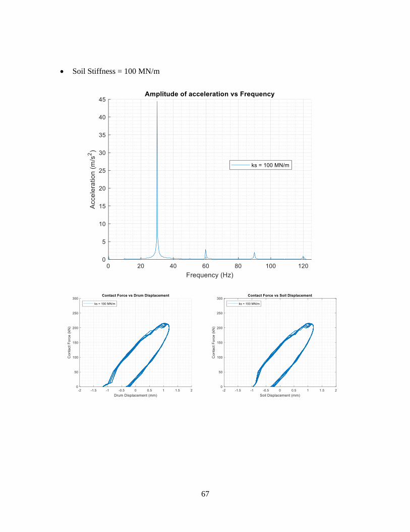
67

• Soil Stiffness = 100 MN/m

68

• Soil Stiffness = 150 MN/m

69

• Soil Stiffness = 200 MN/m

70

Vita

Jesús Castro Pérez was born in Monterrey, Nuevo León, Mexico in 1994. He joined the

Universidad Autónoma de Nuevo León in 2011. During his undergraduate studies participated in

international student competitions organized by the American Concrete Institute, studied a

semester in Spain, and served as an intern at the Secretary of Economy of the State of Nuevo León.

After obtaining an undergraduate degree in civil engineering moved to Chicago to work in a

company that develops instrumentation for nondestructive evaluation of concrete. This experience

ignited and nurtured my interest in concrete technology and nondestructive testing. In 2019 joined

the University of Texas at El Paso and started a master’s degree program. During his studies, he

served as a graduate teaching assistant for Dr. Ivonne Santiago. He wrote his master’s thesis under

the supervision of Dr. Soheil Nazarian.

Permanent email address: [email protected]

This thesis was typed by Jesús Castro Pérez