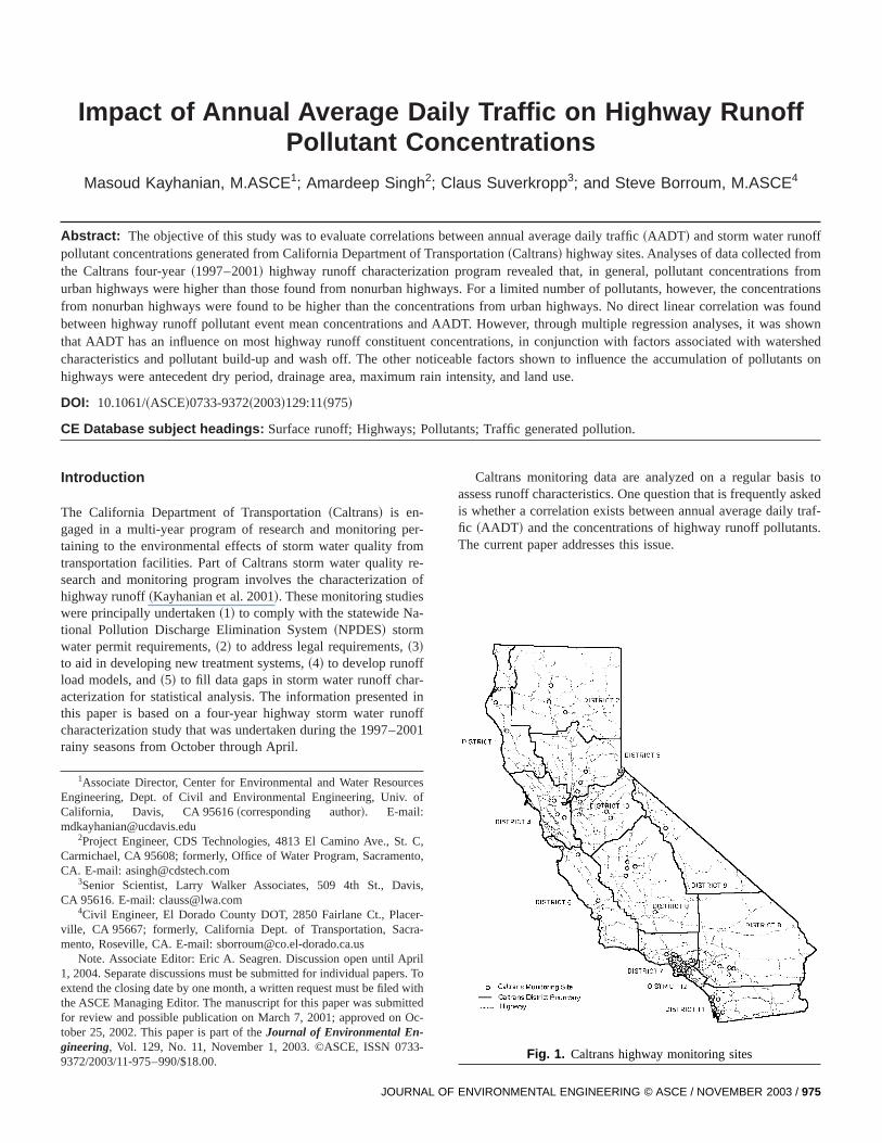
Impact of Annual Average Daily Traffic on Highway Runoff Pollutant Concentrations

Page 1

Impact of Annual Average Daily Traffic on Highway RunoffPollutant Concentrations

Masoud Kayhanian, M.ASCE1; Amardeep Singh2; Claus Suverkropp3; and Steve Borroum, M.ASCE4

fromntrationss found

s showntershedtants on

Abstract: The objective of this study was to evaluate correlations between annual average daily traffic~AADT ! and storm water runoffpollutant concentrations generated from California Department of Transportation~Caltrans! highway sites. Analyses of data collected fromthe Caltrans four-year~1997–2001! highway runoff characterization program revealed that, in general, pollutant concentrationsurban highways were higher than those found from nonurban highways. For a limited number of pollutants, however, the concefrom nonurban highways were found to be higher than the concentrations from urban highways. No direct linear correlation wabetween highway runoff pollutant event mean concentrations and AADT. However, through multiple regression analyses, it wathat AADT has an influence on most highway runoff constituent concentrations, in conjunction with factors associated with wacharacteristics and pollutant build-up and wash off. The other noticeable factors shown to influence the accumulation of polluhighways were antecedent dry period, drainage area, maximum rain intensity, and land use.

DOI: 10.1061/~ASCE!0733-9372~2003!129:11~975!

CE Database subject headings: Surface runoff; Highways; Pollutants; Traffic generated pollution.

emeo

io00

tokedaf-.

ef

Cto

is

r--

ril.i

tec

-

Introduction

The California Department of Transportation~Caltrans! is en-gaged in a multi-year program of research and monitoring ptaining to the environmental effects of storm water quality frotransportation facilities. Part of Caltrans storm water quality rsearch and monitoring program involves the characterizationhighway runoff~Kayhanian et al. 2001!. These monitoring studieswere principally undertaken~1! to comply with the statewide Na-tional Pollution Discharge Elimination System~NPDES! stormwater permit requirements,~2! to address legal requirements,~3!to aid in developing new treatment systems,~4! to develop runoffload models, and~5! to fill data gaps in storm water runoff char-acterization for statistical analysis. The information presentedthis paper is based on a four-year highway storm water runcharacterization study that was undertaken during the 1997–2rainy seasons from October through April.

1Associate Director, Center for Environmental and Water ResourcEngineering, Dept. of Civil and Environmental Engineering, Univ. oCalifornia, Davis, CA 95616~corresponding author!. E-mail:[email protected]

2Project Engineer, CDS Technologies, 4813 El Camino Ave., St.Carmichael, CA 95608; formerly, Office of Water Program, SacramenCA. E-mail: [email protected]

3Senior Scientist, Larry Walker Associates, 509 4th St., DavCA 95616. E-mail: [email protected]

4Civil Engineer, El Dorado County DOT, 2850 Fairlane Ct., Placeville, CA 95667; formerly, California Dept. of Transportation, Sacramento, Roseville, CA. E-mail: [email protected]

Note. Associate Editor: Eric A. Seagren. Discussion open until Ap1, 2004. Separate discussions must be submitted for individual papersextend the closing date by one month, a written request must be filed wthe ASCE Managing Editor. The manuscript for this paper was submitfor review and possible publication on March 7, 2001; approved on Otober 25, 2002. This paper is part of theJournal of Environmental En-gineering, Vol. 129, No. 11, November 1, 2003. ©ASCE, ISSN 07339372/2003/11-975–990/$18.00.

JOURNAL O

r-

-f

nff1

Caltrans monitoring data are analyzed on a regular basisassess runoff characteristics. One question that is frequently asis whether a correlation exists between annual average daily trfic ~AADT ! and the concentrations of highway runoff pollutantsThe current paper addresses this issue.

s

,,

,

Tothd-

Fig. 1. Caltrans highway monitoring sites

F ENVIRONMENTAL ENGINEERING © ASCE / NOVEMBER 2003 / 975

Page 2

000000

00

00

00

000000

0000

00

0

Table 1. Annual Average Daily Traffic Values and other General Characteristics of Monitoring Sites

Highway CountyDrainagearea~ha.! Land use

Annual averagedaily traffic Highway County

Drainagearea~ha.! Land use

Annual averagedaily traffic

580 Alameda 0.1 Transportation 134,000

680 Contra Costa 0.1 Transportation 132,00050 El Dorado 0.3 Residential 37,00050 El Dorado 0.1 Open 14,10050 El Dorado 0.3 Open 11,600180 Fresno 0.7 Transportation 41,00041 Fresno 0.2 Transportation 118,000299 Humboldt 0.1 Residential 8,50036 Humboldt 0.2 Residential 2,600395 Inyo 0.3 Residential 5,50058 Kern 17.3 Transportation 40,000198 Kings 0.1 Agriculture 14,000405 Los Angeles 0.4 Transportation 219,000210 Los Angeles 4.8 Residential 181,000605 Los Angeles 4.1 Agriculture 149,000210 Los Angeles 12.6 Agriculture 97,000210 Los Angeles 0.4 Transportation 176,00091 Los Angeles 0.4 Transportation 187,000105 Los Angeles 0.1 Transportation 218,000210 Los Angeles 12.8 Residential 105,000105 Los Angeles 0.2 Transportation 176,000105 Los Angeles 0.2 Transportation 176,000105 Los Angeles 0.1 Transportation 218,000110 Los Angeles 1.4 Commercial 292,00060 Los Angeles 0.2 Transportation 228,00060 Los Angeles 0.3 Transportation 227,100405 Los Angeles 2.1 Residential 310,000605 Los Angeles 0.1 Transportation 280,000605 Los Angeles 0.0 Transportation 280,00091 Los Angeles 1.0 Commercial 233,0005 Los Angeles 0.1 Transportation 222,000605 Los Angeles 0.1 Transportation 222,000210 Los Angeles 0.2 Transportation 96,00091 Los Angeles 1.6 Industrial 164,000210 Los Angeles 0.4 Transportation 99,000210 Los Angeles 1.5 Residential 128,000101 Los Angeles 1.3 Transportation 328,000405 Los Angeles 1.7 Transportation 260,000405 Los Angeles 0.4 Transportation 322,00010 Los Angeles 1.5 Residential 223,000170 Los Angeles 1.0 Residential 180,000210 Los Angeles 2.9 Residential 126,00010 Los Angeles 0.5 Residential 267,000

170 Los Angeles 0.9 Residential 180,00710 Los Angeles 2.9 Residential 219,00210 Los Angeles 2.8 Commercial 100,00118 Los Angeles 0.8 Residential 111,005 Los Angeles 1.1 Transportation 251,00605 Los Angeles 0.1 Transportation 130,00132 Mariposa 0.3 Residential 2,100101 Mendocino 0.4 Residential 6,400299 Mendocino 0.9 Transportation 1,800142 Orange 0.4 Transportation 16,00405 Orange 0.4 Transportation 237,0080 Placer 0.2 Open 74,00010 Riverside 0.2 Transportation 70,00111 Riverside 0.6 Transportation 13,6010 Riverside 0.5 Residential 18,30010 Riverside 0.2 Residential 63,00099 Sacramento 0.1 Open 47,5050 Sacramento 0.3 Commercial 127,0025 San Benito 0.1 Residential 2,20010 San

Bernardino0.4 Transportation 95,000

805 San Diego 1.1 Transportation 212,008 San Diego 0.2 Transportation 175,005 San Diego 2.1 Transportation 254,0015 San Diego 5.4 Commercial 262,0078 San Diego 1.0 Transportation 112,005 San Diego 1.9 Transportation 188,005 San Diego 1.7 Mixed 182,0005 San Diego 0.9 Transportation 181,0015 San Diego 1.3 Transportation 259,00805 San Diego 0.8 Transportation 177,0012 San Joaquin 0.3 Transportation 14,305 San Joaquin 0.2 Mixed 65,00046 San Luis

Obispo0.5 Residential 21,300

227 San LuisObispo

0.1 Commercial 10,500

1 Santa Cruz 2.4 Residential 55,00680 Solano 0.6 Transportation 53,0036 Tehama 0.6 Transportation 2,1005 Tehama 0.6 Transportation 29,0099 Tulare 0.1 Agriculture 44,500120 Tuolumne 0.3 Residential 4,900

detegehy-eres.siteire

g. 1

c-ansing

, apro-

n-

erent

dis-

Methods

Sampling Procedures

Representative highway sites and storm events were selecteevent-based monitoring. There are a wide range of paramthat can potentially affect the quality of stormwater discharincluding geographic location, climatic/ecologic conditions,drologic conditions, land use, and AADT. The highway sites wselected to represent the full range of physical parameteraddition, the sites were selected as potential monitoringbased on the ability of the sampling teams to perform the requtasks safely. The locations of monitoring sites are shown in Fi

976 / JOURNAL OF ENVIRONMENTAL ENGINEERING © ASCE / NOVEM

forrss

Insd.

As shown in Fig. 1, during the four years of monitoring~1997–2001!, 83 highway sites were monitored for water quality charateristics. These highway sites were located in 7 of the 12 Caltrdistricts. General physical characteristics of these sites, includAADT, are summarized in Table 1.

To ensure monitoring of an appropriate number of stormsweather-tracking procedure was established to target stormsducing a minimum of 2.54 mm of rainfall~7.62 mm in NorthernCalifornia!. The predicted amount of rainfall, known as the quatity of precipitation forecast~QPF!, was obtained from the Na-tional Weather Service in conjunction with other private weathservices up to 72 hours prior to a storm event. Once a storm evwith a targeted QPF was forecasted, monitoring teams were

BER 2003

Page 3

erv

tessterero

0.at

heb-acheivere,itor-ns

di-

n-ltscon-

thehe

an-

ter

ary

s

reend

onalof

nt

patched to the various sites to set up for monitoring and obsthe runoff characteristics.

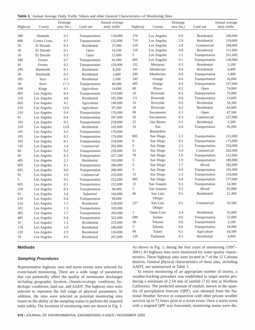
Storm water runoff samples were collected using automasamplers placed at the discharge points downstream of repretative drainage areas. A typical Caltrans automated sampler inlation is shown in Fig. 2. Flow-weighted composite samples wcollected, runoff flow was measured, and rainfall amounts wrecorded using automated equipment. The monitoring was c

Fig. 2. Photo view of typical Caltrans monitoring station

JOURNAL O

e

den-al-een-

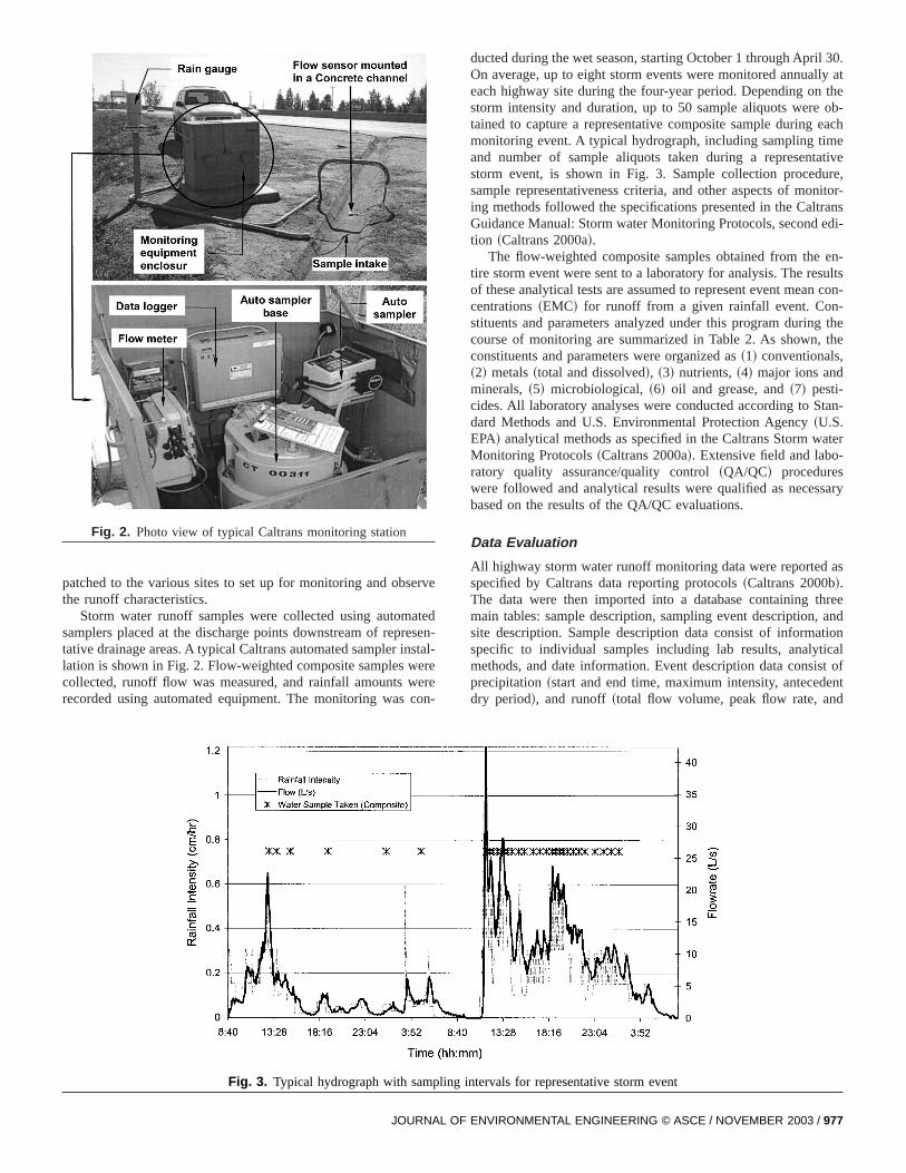
ducted during the wet season, starting October 1 through April 3On average, up to eight storm events were monitored annuallyeach highway site during the four-year period. Depending on tstorm intensity and duration, up to 50 sample aliquots were otained to capture a representative composite sample during emonitoring event. A typical hydrograph, including sampling timand number of sample aliquots taken during a representatstorm event, is shown in Fig. 3. Sample collection procedusample representativeness criteria, and other aspects of moning methods followed the specifications presented in the CaltraGuidance Manual: Storm water Monitoring Protocols, second etion ~Caltrans 2000a!.

The flow-weighted composite samples obtained from the etire storm event were sent to a laboratory for analysis. The resuof these analytical tests are assumed to represent event meancentrations~EMC! for runoff from a given rainfall event. Con-stituents and parameters analyzed under this program duringcourse of monitoring are summarized in Table 2. As shown, tconstituents and parameters were organized as~1! conventionals,~2! metals~total and dissolved!, ~3! nutrients,~4! major ions andminerals,~5! microbiological, ~6! oil and grease, and~7! pesti-cides. All laboratory analyses were conducted according to Stdard Methods and U.S. Environmental Protection Agency~U.S.EPA! analytical methods as specified in the Caltrans Storm waMonitoring Protocols~Caltrans 2000a!. Extensive field and labo-ratory quality assurance/quality control~QA/QC! procedureswere followed and analytical results were qualified as necessbased on the results of the QA/QC evaluations.

Data Evaluation

All highway storm water runoff monitoring data were reported aspecified by Caltrans data reporting protocols~Caltrans 2000b!.The data were then imported into a database containing thmain tables: sample description, sampling event description, asite description. Sample description data consist of informatispecific to individual samples including lab results, analyticmethods, and date information. Event description data consistprecipitation~start and end time, maximum intensity, antecededry period!, and runoff ~total flow volume, peak flow rate, and

Fig. 3. Typical hydrograph with sampling intervals for representative storm event

F ENVIRONMENTAL ENGINEERING © ASCE / NOVEMBER 2003 / 977

Page 4

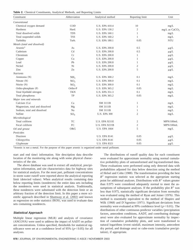
Table 2. Chemical Constituents, Analytical Methods, and Reporting Limits

Constituent Abbreviation Analytical method Reporting limit Unit

ConventionalChemical oxygen demand COD U.S. EPA 410.4 10 mg/LHardness Hard. U.S. EPA 130.2 2 mg/L asCaCO3

Total dissolved solids TDS U.S. EPA 160.1 1 mg/LTotal suspended solids TSS U.S. EPA 160.2 1 mg/LTurbidity Turb. U.S. EPA 180.1 0.05 NTU

Metals (total and dissolved)Arsenica As U.S. EPA 200.8 0.5 mg/LCadmium Cd U.S. EPA 200.8 0.5 mg/LChromium Cr U.S. EPA 200.8 1 mg/LCopper Cu U.S. EPA 200.8 1 mg/LLead Pb U.S. EPA 200.8 1 mg/LNickel Ni U.S. EPA 200.8 2 mg/LZinc Zn U.S. EPA 200.8 5 mg/L

NutrientsAmmonia ~N! NH3 U.S. EPA 300.2 0.1 mg/L

Nitrate ~N! NO3 U.S. EPA 300.0 0.1 mg/L

Nitrite ~N! NO2 U.S. EPA 300.0 0.1 mg/L

Ortho-phosphate~P! Ortho-P U.S. EPA 365.2 0.05 mg/LTotal Kjeldahl nitrogen TKN U.S. EPA 351.3 0.1 mg/LTotal phosphorus TP U.S. EPA 365.2 0.05 mg/L

Major ions and mineralsCalcium ~Ca! Ca SM 3111B 1 mg/LMagnesium, total and dissolved Mg SM 3111B 1 mg/LSodium, total and dissolved Na SM 3111B 1 mg/LSulfate SO4 U.S. EPA 300 2 mg/L

MicrobiologicalTotal coliform TC U.S. EPA 9211E 2 MPN/100mLFecal coliform FC U.S. EPA 9221B 2 MPN/100mL

Oil and grease O&G U.S. EPA 1664 5 mg/L

PesticidesDiazinon U.S. EPA 8141 0.05 mg/LChlorpyrifos U.S. EPA 8141 0.05 mg/LGlyphosate U.S. EPA 8321 0.05 mg/L

aArsenic is not a metal. For the purpose of this paper arsenic is organized under metal pollutant.

eac

cipiteiontintagallyr aci-

ta

eut-si

entula-ata.with

thodstrting

re as-

lity

and

ageec-tont

start and end time! information. Site description data describlocation of the monitoring site along with some physical charteristics of the site.

The above database was used to extract all analytical, pretation information, and site characteristics data for highway sfor statistical analysis. For the most part, pollutant concentratin storm water runoff were reported above the analytical reporlimit ~detected values!. When analytical results containing dabelow reporting limits~nondetects! the entire data sets includinthe nondetects were used in statistical analysis. Traditionthese nondetects were substituted with the detection limit oarbitrary fraction of the detection limit. In this paper a more sentific approach described in Shumway et al.~2002! and knownas regression on order statistics~ROS!, was used to evaluate dasets containing nondetects.

Statistical Approach

Multiple linear regression~MLR! and analysis of covarianc~ANCOVA! were used to address the impact of AADT on pollant concentrations. Unless specified, thresholds for statisticalnificance were set at a confidence level of 95% (p,0.05) for allanalyses.

978 / JOURNAL OF ENVIRONMENTAL ENGINEERING © ASCE / NOVEM

-

i-ssg

,n

g-

The distributions of runoff quality data for each constituwere evaluated for approximate normality using normal cumtive probability plots of untransformed and log-transformed dThese evaluations were performed using only detected dataprobabilities adjusted for data below detection using the meof Helsel and Cohn~1988!. The transformation providing the beR2 regression statistic was selected as the appropriate stapoint for additional analyses. Distributions withR2 values greatethan 0.975 were considered adequately normal to meet thsumptions of subsequent analyses. If the probability plotR2 wasless than 0.975, statistically significant deviation from normawas evaluated using the method of Ryan and Joiner~1976!. Thismethod is essentially equivalent to the method of ShapiroWilk ~1968! and D’Agostino~1971!. Significant deviations fromnormality were evaluated at 99% confidence level (p,0.01). Thedistributions of other continuous predictor variables~precipitationfactors, antecedent conditions, AADT, and contributing drainarea! were also evaluated for approximate normality by insption of cumulative probability plots, and were transformednatural logarithms~event rainfall, maximum intensity, antecededry period, and drainage area! or cube-roots~cumulative precipi-tation!, if appropriate.

BER 2003

Page 5

e

a

o

f

n

h

hn

i

o

t

t

m

l

dna-s,ma-

ap-ith

ffns

on-ra-eshem

ingis

di-y

ely

ol-se-n-oidngper,no

ese

4,ra-d.meofto

DTofex-

on

MLR and ANCOVA methods were used to evaluate the effecof precipitation factors, antecedent conditions, AADT, contribuing drainage area, and surrounding land use on highway runquality. MLR and ANCOVA analyses were performed using onldata reported above reporting limits. Pair-wise comparisons btween land use categories were performed using the TukKramer post-hoc test. MLR models were developed for each costituent. The primary assumptions of MLR analysis~equalvariance and normality! were assessed by inspection of residuplots. Problems due to unequal variance and non-normalityresiduals were largely avoided by transforming dependent aindependent variables to approximate normality prior to analysGenerally, all significant predictor variables (p,0.05) were in-cluded in the MLR model unless they exhibited symptomsmulticollinearity or codependence in the set of predictors. Indpendence of predictor variables~the absence of multicollinearity!was assessed by evaluating correlations and partial correlationthe variables. If correlation coefficients were greater than 0.4a pair of predictors, or if the signs of the correlation and particorrelation coefficients ‘‘disagreed,’’ one of the pair of predictovariables was excluded from the MLR model. Partial correlatiowere also used to select the independent variables for the Mmodels.

The final ‘‘optimized’’ MLR model was used to generate anew fitted variable calculated as the cumulative effects of tsignificant predictor variables for each constituent. This fittevariable was then included as the single covariate in tANCOVA models used to evaluate the effects of surrounding lause. Because of imbalances in the representation of land useegories, interaction between individual covariates in the MLmodel and the categorical variables could not be assessedstatistically rigorous way. Instead, potential interaction effecwere quantitatively evaluated by inspection of bivariate plotsthe dependent variable versus the MLR-fitted data. In all casinteraction was judged to be minimal and to have no substaneffect on the interpretation of the ANCOVA results.

Results and Discussion

Highway Classification

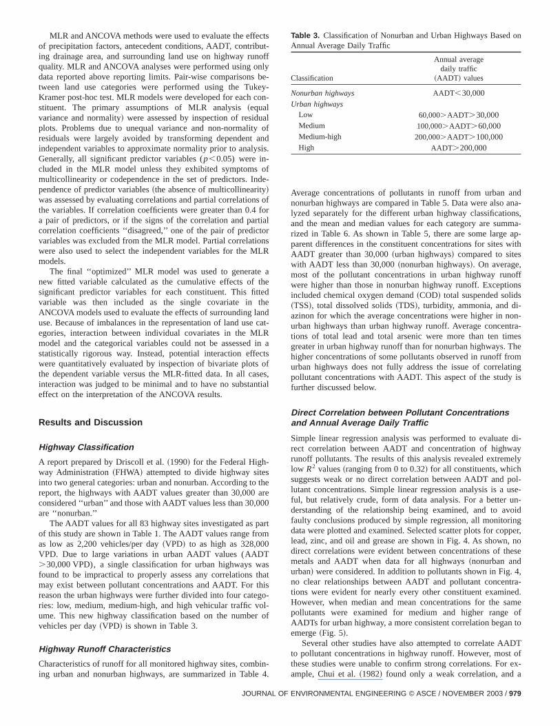
A report prepared by Driscoll et al.~1990! for the Federal High-way Administration~FHWA! attempted to divide highway sitesinto two general categories: urban and nonurban. According toreport, the highways with AADT values greater than 30,000 aconsidered ‘‘urban’’ and those with AADT values less than 30,00are ‘‘nonurban.’’

The AADT values for all 83 highway sites investigated as paof this study are shown in Table 1. The AADT values range froas low as 2,200 vehicles/per day~VPD! to as high as 328,000VPD. Due to large variations in urban AADT values (AADT.30,000 VPD), a single classification for urban highways wafound to be impractical to properly assess any correlations thmay exist between pollutant concentrations and AADT. For threason the urban highways were further divided into four categries: low, medium, medium-high, and high vehicular traffic voume. This new highway classification based on the numbervehicles per day~VPD! is shown in Table 3.

Highway Runoff Characteristics

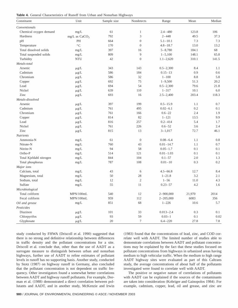
Characteristics of runoff for all monitored highway sites, combining urban and nonurban highways, are summarized in Table

JOURNAL O

tst-offye-y-n-

lofndis.

fe-

s oforalrs

LR

eded

cat-Rn atsf

es,ial

here0

rt

satiso--of

-4.

Average concentrations of pollutants in runoff from urban annonurban highways are compared in Table 5. Data were also alyzed separately for the different urban highway classificationand the mean and median values for each category are sumrized in Table 6. As shown in Table 5, there are some largeparent differences in the constituent concentrations for sites wAADT greater than 30,000~urban highways! compared to siteswith AADT less than 30,000~nonurban highways!. On average,most of the pollutant concentrations in urban highway runowere higher than those in nonurban highway runoff. Exceptioincluded chemical oxygen demand~COD! total suspended solids~TSS!, total dissolved solids~TDS!, turbidity, ammonia, and di-azinon for which the average concentrations were higher in nurban highways than urban highway runoff. Average concenttions of total lead and total arsenic were more than ten timgreater in urban highway runoff than for nonurban highways. Thigher concentrations of some pollutants observed in runoff frourban highways does not fully address the issue of correlatpollutant concentrations with AADT. This aspect of the studyfurther discussed below.

Direct Correlation between Pollutant Concentrationsand Annual Average Daily Traffic

Simple linear regression analysis was performed to evaluaterect correlation between AADT and concentration of highwarunoff pollutants. The results of this analysis revealed extremlow R2 values~ranging from 0 to 0.32! for all constituents, whichsuggests weak or no direct correlation between AADT and plutant concentrations. Simple linear regression analysis is a uful, but relatively crude, form of data analysis. For a better uderstanding of the relationship being examined, and to avfaulty conclusions produced by simple regression, all monitoridata were plotted and examined. Selected scatter plots for coplead, zinc, and oil and grease are shown in Fig. 4. As shown,direct correlations were evident between concentrations of thmetals and AADT when data for all highways~nonurban andurban! were considered. In addition to pollutants shown in Fig.no clear relationships between AADT and pollutant concenttions were evident for nearly every other constituent examineHowever, when median and mean concentrations for the sapollutants were examined for medium and higher rangeAADTs for urban highway, a more consistent correlation beganemerge~Fig. 5!.

Several other studies have also attempted to correlate AAto pollutant concentrations in highway runoff. However, mostthese studies were unable to confirm strong correlations. Forample, Chui et al.~1982! found only a weak correlation, and a

Table 3. Classification of Nonurban and Urban Highways BasedAnnual Average Daily Traffic

Classification

Annual averagedaily traffic

~AADT ! values

Nonurban highways AADT,30,000Urban highways

Low 60,000.AADT.30,000Medium 100,000.AADT.60,000Medium-high 200,000.AADT.100,000High AADT.200,000

F ENVIRONMENTAL ENGINEERING © ASCE / NOVEMBER 2003 / 979

Page 6

n

Table 4. General Characteristics of Runoff from Urban and Nonurban Highways

Constituent Unit Sample size Nondetects Range Mean Media

ConventionalsChemical oxygen demand mg/L 61 1 2.4–480 123.8 106Hardness mg/L asCaCO3 792 3 2–448 49.5 37.3

pH PH 664 0 5.1–10.1 7.3 7.3Temperature °C 170 0 4.8–18.7 13.0 13.2

Total dissolved solids mg/L 397 16 5–8,780 184.1 68Total suspended solids mg/L 809 9 1–5,100 148.1 65.8Turbidity NTU 42 0 1.1–2,620 310.1 141.5

Metals-totalArsenic mg/L 343 143 0.5–2,300 8.4 1.1Cadmium mg/L 586 184 0.15–13 0.9 0.6Chromium mg/L 586 32 1–100 8.8 5.8Copper mg/L 692 75 1–9,500 51.3 20.2Lead mg/L 694 54 0.5–2,300 79.6 21.8Nickel mg/L 639 110 1–317 10.1 6.0Zinc mg/L 693 16 2.5–2,400 203.4 118.3

Metals-dissolvedArsenic mg/L 397 199 0.5–15.9 1.1 0.7Cadmium mg/L 761 495 0.02–6.1 0.2 0.1Chromium mg/L 761 166 0.6–22 2.4 1.9Copper mg/L 814 82 1–121 13.5 9.9Lead mg/L 816 257 0.2–414 5.4 1.7Nickel mg/L 761 226 0.6–52 3.6 2.4Zinc mg/L 815 13 3–1,017 72.7 46.1

NutrientsAmmonia-N mg/L 61 0 0.08–6.4 1.1 0.8Nitrate-N mg/L 760 43 0.01–14.7 1.1 0.7Nitrite-N mg/L 94 58 0.05–1.7 0.1 0.1Ortho-P mg/L 514 121 0.01–1.03 0.1 0.1Total Kjeldahl nitrogen mg/L 844 104 0.1–57 2.0 1.3Total phosphorus mg/L 787 108 0.01–10 0.3 0.2

Major ionsCalcium, total mg/L 43 6 4.5–66.8 12.7 8.4Magnesium, total mg/L 50 28 1–21.8 3.2 2.1Sodium, total mg/L 12 2 1–56 11.0 4.3Sulfate mg/L 55 11 0.23–57 4.2 1.6

MicrobiologicalTotal coliform MPN/100mL 540 12 2–900,000 21,970 2014Fecal coliform MPN/100mL 959 112 2–205,000 6083 356

Oil and grease mg/L 851 68 1–226 10.6 5.7

PesticidesDiazinon mg/L 101 33 0.013–2.4 0.3 0.1Chlorpyrifos mg/L 93 59 0.03–1 0.1 0.02Glyphosate mg/L 20 7 6.4–220 27.8 7.8

t

is

aceftioo

or-otra-

oninggensnts

tsts

are

study conducted by FHWA~Driscoll et al. 1990! suggested thathere is no strong and definitive relationship between differenin traffic density and the pollutant concentrations for a sDriscoll et al. conclude that, other than the use of AADT asurrogate measure to distinguish between urban and nonuhighways, further use of AADT to refine estimates of pollutlevels in runoff has no supporting basis. Another study, conduby Stotz ~1987! on highway runoff in Germany, also concludthat the pollutant concentration is not dependent on trafficquency. Other investigators found a somewhat better correlabetween AADT and highway runoff pollutants. For example, Dman et al.~1988! demonstrated a direct correlation between plutants and AADT, and in another study, McKenzie and Irw

980 / JOURNAL OF ENVIRONMENTAL ENGINEERING © ASCE / NOVE

ceste.

arbanntteddre-onsr-l-

in

~1983! found that the concentrations of lead, zinc, and COD crelate well with AADT. The limited number of studies able tdemonstrate correlations between AADT and pollutant concentions may be explained by the fact that these studies focusedpollutant concentrations from highways in urbanized areas havmedium to high vehicular traffic. When the medium to high ranAADT highway sites were evaluated as part of this Caltrastudy, the average concentrations of about half of the pollutainvestigated were found to correlate well with AADT.

The positive or negative nature of correlations of pollutanwith AADT can be explained if the sources of the contaminanare taken into consideration~Kobriger and Gainopolos 1984!. Forexample, cadmium, copper, lead, oil and grease, and zinc

MBER 2003

Page 7

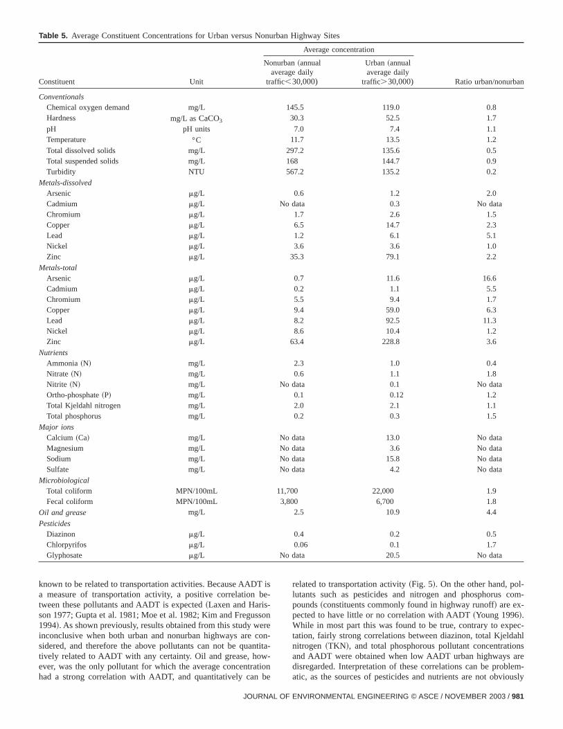
Table 5. Average Constituent Concentrations for Urban versus Nonurban Highway Sites

Constituent Unit

Average concentration

Ratio urban/nonurban

Nonurban~annualaverage daily

traffic,30,000)

Urban ~annualaverage daily

traffic.30,000)

ConventionalsChemical oxygen demand mg/L 145.5 119.0 0.8Hardness mg/L asCaCO3 30.3 52.5 1.7

pH pH units 7.0 7.4 1.1Temperature °C 11.7 13.5 1.2

Total dissolved solids mg/L 297.2 135.6 0.5Total suspended solids mg/L 168 144.7 0.9Turbidity NTU 567.2 135.2 0.2

Metals-dissolvedArsenic mg/L 0.6 1.2 2.0Cadmium mg/L No data 0.3 No dataChromium mg/L 1.7 2.6 1.5Copper mg/L 6.5 14.7 2.3Lead mg/L 1.2 6.1 5.1Nickel mg/L 3.6 3.6 1.0Zinc mg/L 35.3 79.1 2.2

Metals-totalArsenic mg/L 0.7 11.6 16.6Cadmium mg/L 0.2 1.1 5.5Chromium mg/L 5.5 9.4 1.7Copper mg/L 9.4 59.0 6.3Lead mg/L 8.2 92.5 11.3Nickel mg/L 8.6 10.4 1.2Zinc mg/L 63.4 228.8 3.6

NutrientsAmmonia ~N! mg/L 2.3 1.0 0.4Nitrate ~N! mg/L 0.6 1.1 1.8Nitrite ~N! mg/L No data 0.1 No dataOrtho-phosphate~P! mg/L 0.1 0.12 1.2Total Kjeldahl nitrogen mg/L 2.0 2.1 1.1Total phosphorus mg/L 0.2 0.3 1.5

Major ionsCalcium ~Ca! mg/L No data 13.0 No dataMagnesium mg/L No data 3.6 No dataSodium mg/L No data 15.8 No dataSulfate mg/L No data 4.2 No data

MicrobiologicalTotal coliform MPN/100mL 11,700 22,000 1.9Fecal coliform MPN/100mL 3,800 6,700 1.8

Oil and grease mg/L 2.5 10.9 4.4

PesticidesDiazinon mg/L 0.4 0.2 0.5Chlorpyrifos mg/L 0.06 0.1 1.7Glyphosate mg/L No data 20.5 No data

ibe

soreoti-

iobe

om-

c-hlnsreem-usly

known to be related to transportation activities. Because AADTa measure of transportation activity, a positive correlationtween these pollutants and AADT is expected~Laxen and Haris-son 1977; Gupta et al. 1981; Moe et al. 1982; Kim and Fregus1994!. As shown previously, results obtained from this study weinconclusive when both urban and nonurban highways are csidered, and therefore the above pollutants can not be quantively related to AADT with any certainty. Oil and grease, however, was the only pollutant for which the average concentrathad a strong correlation with AADT, and quantitatively can

JOURNAL O

s-

n

n-ta-

n

related to transportation activity~Fig. 5!. On the other hand, pol-lutants such as pesticides and nitrogen and phosphorus cpounds~constituents commonly found in highway runoff! are ex-pected to have little or no correlation with AADT~Young 1996!.While in most part this was found to be true, contrary to expetation, fairly strong correlations between diazinon, total Kjeldanitrogen ~TKN!, and total phosphorous pollutant concentratioand AADT were obtained when low AADT urban highways adisregarded. Interpretation of these correlations can be problatic, as the sources of pesticides and nutrients are not obvio

F ENVIRONMENTAL ENGINEERING © ASCE / NOVEMBER 2003 / 981

Page 8

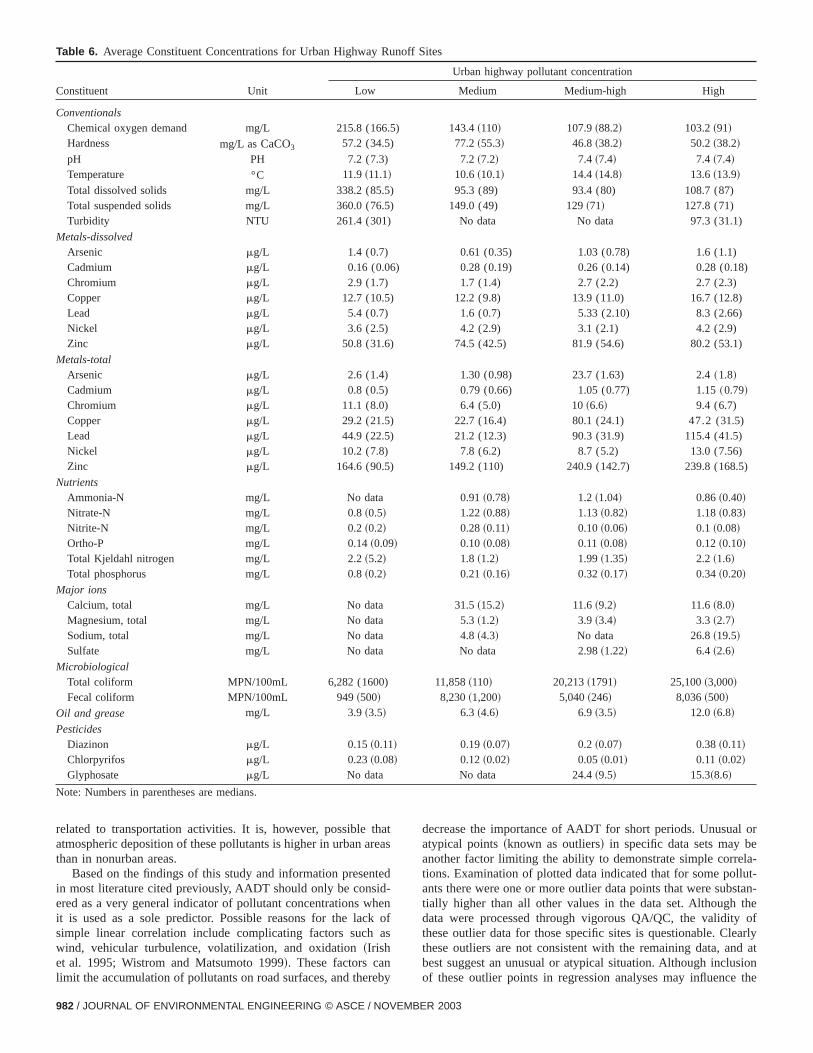
Table 6. Average Constituent Concentrations for Urban Highway Runoff Sites

Constituent Unit

Urban highway pollutant concentration

Low Medium Medium-high High

ConventionalsChemical oxygen demand mg/L 215.8 (166.5) 143.4~110! 107.9~88.2! 103.2~91!

Hardness mg/L asCaCO3 57.2 (34.5) 77.2~55.3! 46.8~38.2! 50.2~38.2!

pH PH 7.2 (7.3) 7.2~7.2! 7.4 ~7.4! 7.4 ~7.4!Temperature °C 11.9~11.1! 10.6~10.1! 14.4~14.8! 13.6~13.9!

Total dissolved solids mg/L 338.2 (85.5) 95.3 (89) 93.4 (80) 108.7 (87)Total suspended solids mg/L 360.0 (76.5) 149.0 (49) 129~71! 127.8 (71)Turbidity NTU 261.4 (301) No data No data 97.3 (31.1)

Metals-dissolvedArsenic mg/L 1.4 (0.7) 0.61 (0.35) 1.03 (0.78) 1.6 (1.1)Cadmium mg/L 0.16 (0.06) 0.28 (0.19) 0.26 (0.14) 0.28 (0.18)Chromium mg/L 2.9 (1.7) 1.7 (1.4) 2.7 (2.2) 2.7 (2.3)Copper mg/L 12.7 (10.5) 12.2 (9.8) 13.9 (11.0) 16.7 (12.8)Lead mg/L 5.4 (0.7) 1.6 (0.7) 5.33 (2.10) 8.3 (2.66)Nickel mg/L 3.6 (2.5) 4.2 (2.9) 3.1 (2.1) 4.2 (2.9)Zinc mg/L 50.8 (31.6) 74.5 (42.5) 81.9 (54.6) 80.2 (53.1)

Metals-totalArsenic mg/L 2.6 (1.4) 1.30 (0.98) 23.7 (1.63) 2.4~1.8!

Cadmium mg/L 0.8 (0.5) 0.79 (0.66) 1.05 (0.77) 1.15~0.79!Chromium mg/L 11.1 (8.0) 6.4 (5.0) 10~6.6! 9.4 (6.7)Copper mg/L 29.2 (21.5) 22.7 (16.4) 80.1 (24.1) 47.2 (31.5)Lead mg/L 44.9 (22.5) 21.2 (12.3) 90.3 (31.9) 115.4 (41.5)Nickel mg/L 10.2 (7.8) 7.8 (6.2) 8.7 (5.2) 13.0 (7.56)Zinc mg/L 164.6 (90.5) 149.2 (110) 240.9 (142.7) 239.8 (168.5)

NutrientsAmmonia-N mg/L No data 0.91~0.78! 1.2 ~1.04! 0.86~0.40!Nitrate-N mg/L 0.8~0.5! 1.22~0.88! 1.13~0.82! 1.18~0.83!Nitrite-N mg/L 0.2~0.2! 0.28~0.11! 0.10~0.06! 0.1 ~0.08!Ortho-P mg/L 0.14~0.09! 0.10~0.08! 0.11~0.08! 0.12~0.10!Total Kjeldahl nitrogen mg/L 2.2~5.2! 1.8 ~1.2! 1.99~1.35! 2.2 ~1.6!Total phosphorus mg/L 0.8~0.2! 0.21~0.16! 0.32~0.17! 0.34~0.20!

Major ionsCalcium, total mg/L No data 31.5~15.2! 11.6~9.2! 11.6~8.0!Magnesium, total mg/L No data 5.3~1.2! 3.9 ~3.4! 3.3 ~2.7!Sodium, total mg/L No data 4.8~4.3! No data 26.8~19.5!Sulfate mg/L No data No data 2.98~1.22! 6.4 ~2.6!

MicrobiologicalTotal coliform MPN/100mL 6,282 (1600) 11,858~110! 20,213~1791! 25,100~3,000!Fecal coliform MPN/100mL 949~500! 8,230~1,200! 5,040~246! 8,036~500!

Oil and grease mg/L 3.9~3.5! 6.3 ~4.6! 6.9 ~3.5! 12.0~6.8!

PesticidesDiazinon mg/L 0.15~0.11! 0.19~0.07! 0.2 ~0.07! 0.38~0.11!Chlorpyrifos mg/L 0.23~0.08! 0.12~0.02! 0.05~0.01! 0.11~0.02!Glyphosate mg/L No data No data 24.4~9.5! 15.3~8.6!

Note: Numbers in parentheses are medians.

aa

e-eos

b

or

a-t-

tan-eofrlyat

onthe

related to transportation activities. It is, however, possible thatmospheric deposition of these pollutants is higher in urban arethan in nonurban areas.

Based on the findings of this study and information presentin most literature cited previously, AADT should only be considered as a very general indicator of pollutant concentrations whit is used as a sole predictor. Possible reasons for the lacksimple linear correlation include complicating factors such awind, vehicular turbulence, volatilization, and oxidation~Irishet al. 1995; Wistrom and Matsumoto 1999!. These factors canlimit the accumulation of pollutants on road surfaces, and there

982 / JOURNAL OF ENVIRONMENTAL ENGINEERING © ASCE / NOVEM

ts

d

nf

y

decrease the importance of AADT for short periods. Unusualatypical points~known as outliers! in specific data sets may beanother factor limiting the ability to demonstrate simple correltions. Examination of plotted data indicated that for some polluants there were one or more outlier data points that were substially higher than all other values in the data set. Although thdata were processed through vigorous QA/QC, the validitythese outlier data for those specific sites is questionable. Cleathese outliers are not consistent with the remaining data, andbest suggest an unusual or atypical situation. Although inclusiof these outlier points in regression analyses may influence

BER 2003

Page 9

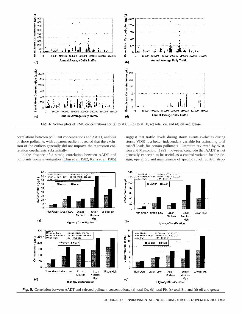
Fig. 4. Scatter plots of EMC concentrations for~a! total Cu,~b! total Pb,~c! total Zn, and~d! oil and grease

lysclu

co

an

talt-

tde-uc-

correlations between pollutant concentrations and AADT, anaof those pollutants with apparent outliers revealed that the exsion of the outliers generally did not improve the regressionrelation coefficients substantially.

In the absence of a strong correlation between AADTpollutants, some investigators~Chui et al. 1982; Kerri et al. 1985!

JOURNAL O

is-

r-

d

suggest that traffic levels during storm events~vehicles duringstorm, VDS! is a better independent variable for estimating torunoff loads for certain pollutants. Literature reviewed by Wisrom and Matsomoto~1999!, however, conclude that AADT is nogenerally expected to be useful as a control variable for thesign, operation, and maintenance of specific runoff control str

Fig. 5. Correlation between AADT and selected pollutant concentrations,~a! total Cu,~b! total Pb,~c! total Zn, and~d! oil and grease

F ENVIRONMENTAL ENGINEERING © ASCE / NOVEMBER 2003 / 983

Page 10

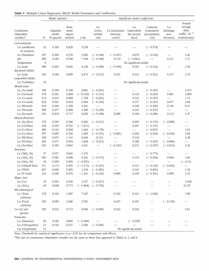
Table 7. Multiple Linear Regression~MLR! Model Parameters and Coefficients

Constituent~dependentvariable!a

Model statistics Significant model coefficients

N

Adjustedmodel

R-squared

Rootmeansquare

residual y-Int.

Ln@event

rainfall,cm#

Ln @maximumintensity,cm/hr#

Ln@antecedentdry period,

days#

Cuberoot@cumulativeprecipitation,

cm#

Ln@drainage

area,hectares#

Annualaveragedaily

traffic•1026

~vehicles/day!

ConventionalsLn ~coefficient

of variance!52 0.169 0.820 5.259 — — — (20.379) — —

Ln ~Hardness! 597 0.300 0.576 3.585 (20.189) (20.107) 0.076 (20.150) — 2.45pH 499 0.183 0.568 7.344 (20.248) 0.133 (20.061) — 0.111 1.71Temperature 9 No significant modelLn ~total

dissolved solids!309 0.303 0.645 4.238 (20.308) (20.109) 0.105 (20.124) — 2.38

Ln ~totalsuspended solids!

592 0.186 0.999 4.472 (20.213) 0.101 0.155 (20.321) 0.157 2.19

Ln ~Turbidity! 19 No significant model

Metals-totalLn ~As-total! 189 0.196 0.548 0.865 (20.201) — — (20.187) — 2.075Ln ~Cd-total! 479 0.281 0.684 (20.129) (20.131) — 0.129 (20.343) 0.081 2.893Ln ~Cr-total! 574 0.213 0.688 1.709 (20.205) — 0.110 (20.197) — 1.73Ln ~Cu-total! 626 0.501 0.654 2.944 (20.230) — 0.127 (20.247) 0.077 5.66Ln ~Pb-total! 619 0.346 1.209 2.441 — — 0.148 (20.340) 0.130 9.21Ln ~Ni-total! 560 0.257 0.649 2.386 (20.238) — 0.161 (20.235) — —Ln ~Zn-total! 591 0.454 0.717 4.650 (20.198) 0.080 0.164 (20.286) 0.113 5.37

Metals-dissolvedLn ~As-Diss! 176 0.205 0.546 0.492 (20.121) — 0.093 (20.176) (20.090) —Ln ~Cd-Diss! 254 0.103 0.762 (21.411) — — 0.207 (20.131) — —Ln ~Cr-Diss! 480 0.132 0.504 1.042 (20.178) — — (20.097) — 1.02Ln ~Cu-Diss! 597 0.485 0.520 1.943 (20.222) (20.081) 0.204 (20.204) (20.036) 2.96Ln ~Pb-Diss! 548 0.037 1.131 0.444 0.133 — 0.120 — — 2.38Ln ~Ni-Diss! 456 0.271 0.583 1.428 (20.221) — 0.186 (20.183) (20.040) —Ln ~Zn-Diss! 591 0.185 0.843 3.411 — (20.122) 0.231 (20.197) (20.053) 2.22

Nutrients

Ln (NH3-N) 57 0.557 0.642 1.353 — — — (20.775) — —

Ln (NO3-N) 585 0.381 0.608 0.202 (20.373) — 0.119 (20.264) 0.044 1.60

Ln (NO2-N) 34 0.309 0.569 (20.955) — — — — — (24.12)

Ln ~OrthoP-Diss! 371 0.173 0.595 (22.173) (20.187) — 0.121 (20.120) (20.043) —Ln ~TKN! 607 0.440 0.585 1.159 (20.285) — 0.141 (20.405) — 1.34Ln ~P-Total! 521 0.296 0.676 21.101 (20.216) 0.084 0.109 (20.301) 0.090 2.25

Major ionsLn ~Ca! 33 0.392 0.450 2.237 (20.427) — — — — 2.209

Ln (SO4) 44 0.648 0.773 (22.464) (20.730) — — — — 21.39

MicrobiologicalLn ~Total

coliform!278 0.194 1.687 7.547 — 0.192 0.321 (21.030) — 7.88

Ln ~Fecalcoliform!

595 0.085 2.046 5.591 — 0.247 0.347 — (20.159) —

Ln ~oil andgrease!

336 0.552 0.712 0.846 (20.560) 0.322 0.254 — — 5.61

PesticidesLn ~Diazinon! 30 0.186 0.895 (20.369) — — (20.328) — — —Ln ~Chlorpyrifos! 21 0.156 0.557 22.586 (20.506) — — — — —Ln ~Glyphosate! 12 No significant model

Note: Threshold for statistical significance isp,0.05 for all comparisons and effects.aThe unit of constituents~dependent variable! are the same as those that appeared in Tables 4, 5, and 6.

984 / JOURNAL OF ENVIRONMENTAL ENGINEERING © ASCE / NOVEMBER 2003

Page 11

s

Table 8. Summary of Significant Effects for Multiple Linear Regression Models

Covariate factor~predictor variable!

Dominant effect on pollutantconcentrationsa

Ratio of models exhibitingsignificant dominant effectb Exceptionsc Comments

Event rainfall Concentrations decrease withhigher total event rainfall

23 of 24 models had asignificant negativecoefficient

Positive: dissolved Pb;Not significant: total Pb,dissolved Zn, chemical oxygendemand, NH3, NO2 , fecaland total coliform, diazinon

Very consistent predictor.Same pattern for nearlyall models.

Maximum rainfallintensity

Concentrations increase withhigher maximum intensity

7 of 11 models had asignificant positivecoefficient

Negative: dissolved Cu and Zn,hardness, total dissolved solids

Not significantis themost common result.Maximum intensity iscorrelated with eventrainfall. Generallyappears not to be agood predictor variable.

Antecedent dryperiod

Concentrations increase withlonger antecedent dry period

23 of 25 models had asignificant positivecoefficient

Negative: pH, diazinon;Not significant: total As,dissolved Cr, Calcium, chemicaloxygen demand, SO4 , NH3,

NO2 , and chlorpyrifos

Very consistent predictor.Same pattern for nearlyall significant models.

Seasonal cumulativeprecipitation

Concentrations decrease ascumulative rainfall increases

24 of 24 models had asignificant negativecoefficient

Positive: noneNot significant: dissolved Pb,calcium, oil and grease,pH, SO4 , turbidity, NO2 ,fecal coliform, chlorpyrifosand diazinon

Very consistent predictor.Same pattern for allsignificant models.

Drainage area Concentrations are higherfor larger drainage areas

9 of 15 models had asignificant positivecoefficient

Negative: dissolved As, Cu,Ni, and Zn, dissolvedorthophosphate, and fecalcoliform

Positive for total metals,total P, and TSS. Negativeor not significantfor dissolved metals anddissolved ortho-P.

Annual averagedaily traffic

Concentrations are higherfor sites with higher traffic

22 of 23 models had asignificant positivecoefficient

Negative: NO2

Not significant: dissolvedAs, Cd, and Ni, total Ni,chemical oxygen demand,NH3 , ortho-P, fecalcoliform, chlorpyrifosand diazinon

Very consistent predictor.Same pattern for nearly allsignificant models.

aSummarized for multiple linear regression models including only whole storm or first flush data. ‘‘Dominant effect’’ is the most frequently observedignof significant coefficients for the factor in multiple linear regression models. In all cases, the relationship between covariate and dependent variables~aftertransforming to approximate normality! is approximately linear.bThreshold of statistical significance isp,0.05.cConstituents for which the predictor had a significant effect opposite to the dominant effect for the predictor.

t

lurga

t

ta-

ts.

t-s

n-

tures, as traffic intensity on a particular stretch of highwayexpected to be fairly constant from day to day.

From the discussion above, it appears that the AADT is notsole factor contributing to pollutant accumulation in highwasites. In the absence of a direct relationship between AADT ahighway runoff pollutants, the search for a better model shiftedmultiple regression, where variables other than AADT were cosidered.

Multiple Linear Regression Analysis

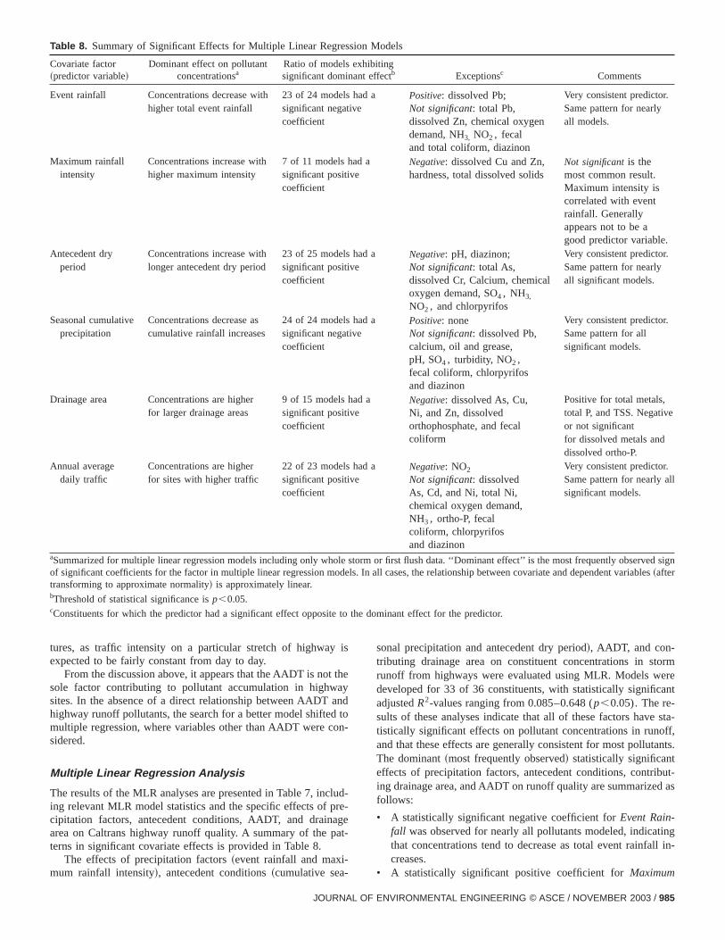
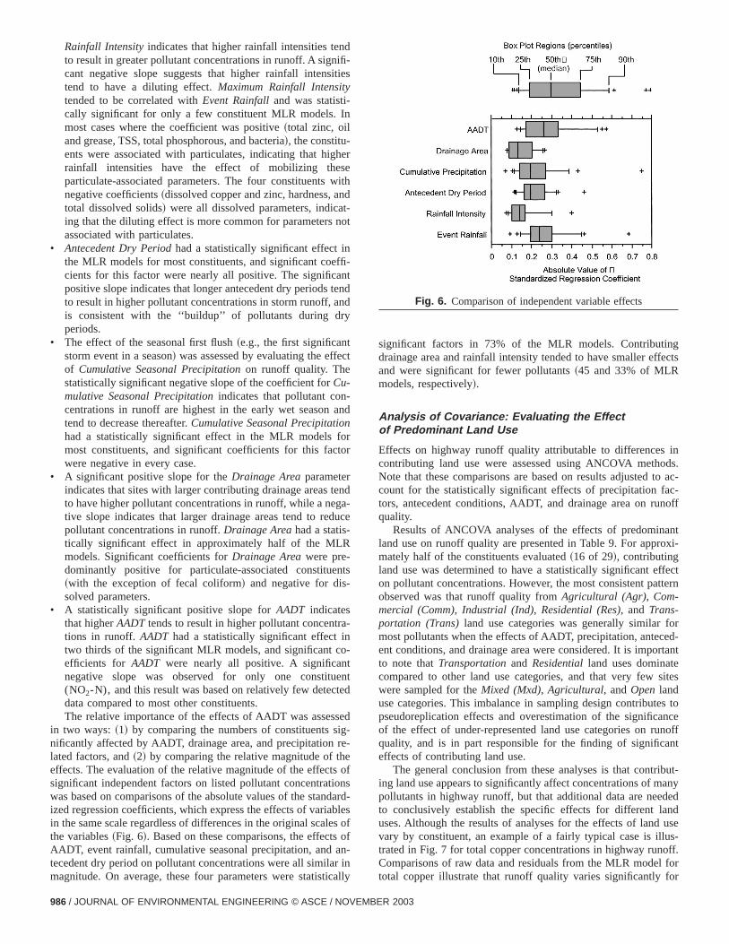
The results of the MLR analyses are presented in Table 7, incing relevant MLR model statistics and the specific effects of pcipitation factors, antecedent conditions, AADT, and drainaarea on Caltrans highway runoff quality. A summary of the pterns in significant covariate effects is provided in Table 8.

The effects of precipitation factors~event rainfall and maxi-mum rainfall intensity!, antecedent conditions~cumulative sea-

JOURNAL

is

heyndton-

d-e-et-

sonal precipitation and antecedent dry period!, AADT, and con-tributing drainage area on constituent concentrations in stormrunoff from highways were evaluated using MLR. Models weredeveloped for 33 of 36 constituents, with statistically significanadjustedR2-values ranging from 0.085–0.648 (p,0.05). The re-sults of these analyses indicate that all of these factors have stistically significant effects on pollutant concentrations in runoff,and that these effects are generally consistent for most pollutanThe dominant~most frequently observed! statistically significanteffects of precipitation factors, antecedent conditions, contribuing drainage area, and AADT on runoff quality are summarized afollows:

• A statistically significant negative coefficient forEvent Rain-fall was observed for nearly all pollutants modeled, indicatingthat concentrations tend to decrease as total event rainfall icreases.

• A statistically significant positive coefficient forMaximum

OF ENVIRONMENTAL ENGINEERING © ASCE / NOVEMBER 2003 / 985

Page 12

ndifi-itie

In

hesewindt-no

nffi-nttennd

y

tect

-annfortor

tengaduc

R

nts-

ra-no-tented

sedig-re-

hes oiondableess oan-r inica

cts

s.ac-

-off

txi-

ctern

rd-ant

tes

toceofft

ut-nyd

dse-f.orr

Rainfall Intensityindicates that higher rainfall intensities teto result in greater pollutant concentrations in runoff. A signcant negative slope suggests that higher rainfall intenstend to have a diluting effect.Maximum Rainfall Intensitytended to be correlated withEvent Rainfalland was statisti-cally significant for only a few constituent MLR models.most cases where the coefficient was positive~total zinc, oiland grease, TSS, total phosphorous, and bacteria!, the constitu-ents were associated with particulates, indicating that higrainfall intensities have the effect of mobilizing theparticulate-associated parameters. The four constituentsnegative coefficients~dissolved copper and zinc, hardness, atotal dissolved solids! were all dissolved parameters, indicaing that the diluting effect is more common for parametersassociated with particulates.

• Antecedent Dry Periodhad a statistically significant effect ithe MLR models for most constituents, and significant coecients for this factor were nearly all positive. The significapositive slope indicates that longer antecedent dry periodsto result in higher pollutant concentrations in storm runoff, ais consistent with the ‘‘buildup’’ of pollutants during drperiods.

• The effect of the seasonal first flush~e.g., the first significanstorm event in a season! was assessed by evaluating the effof Cumulative Seasonal Precipitationon runoff quality. Thestatistically significant negative slope of the coefficient forCu-mulative Seasonal Precipitationindicates that pollutant concentrations in runoff are highest in the early wet seasontend to decrease thereafter.Cumulative Seasonal Precipitatiohad a statistically significant effect in the MLR modelsmost constituents, and significant coefficients for this facwere negative in every case.

• A significant positive slope for theDrainage Areaparameterindicates that sites with larger contributing drainage areasto have higher pollutant concentrations in runoff, while a netive slope indicates that larger drainage areas tend to repollutant concentrations in runoff.Drainage Areahad a statis-tically significant effect in approximately half of the MLmodels. Significant coefficients forDrainage Areawere pre-dominantly positive for particulate-associated constitue~with the exception of fecal coliform! and negative for dissolved parameters.

• A statistically significant positive slope forAADT indicatesthat higherAADT tends to result in higher pollutant concenttions in runoff. AADT had a statistically significant effect itwo thirds of the significant MLR models, and significant cefficients for AADT were nearly all positive. A significannegative slope was observed for only one constitu(NO2-N), and this result was based on relatively few detecdata compared to most other constituents.The relative importance of the effects of AADT was asses

in two ways:~1! by comparing the numbers of constituents snificantly affected by AADT, drainage area, and precipitationlated factors, and~2! by comparing the relative magnitude of teffects. The evaluation of the relative magnitude of the effectsignificant independent factors on listed pollutant concentratwas based on comparisons of the absolute values of the stanized regression coefficients, which express the effects of variain the same scale regardless of differences in the original scalthe variables~Fig. 6!. Based on these comparisons, the effectAADT, event rainfall, cumulative seasonal precipitation, andtecedent dry period on pollutant concentrations were all similamagnitude. On average, these four parameters were statist

986 / JOURNAL OF ENVIRONMENTAL ENGINEERING © ASCE / NOVEM

s

r

th

t

d

d

d-e

t

fsrd-soff

lly

significant factors in 73% of the MLR models. Contributingdrainage area and rainfall intensity tended to have smaller effeand were significant for fewer pollutants~45 and 33% of MLRmodels, respectively!.

Analysis of Covariance: Evaluating the Effectof Predominant Land Use

Effects on highway runoff quality attributable to differences incontributing land use were assessed using ANCOVA methodNote that these comparisons are based on results adjusted tocount for the statistically significant effects of precipitation factors, antecedent conditions, AADT, and drainage area on runquality.

Results of ANCOVA analyses of the effects of predominanland use on runoff quality are presented in Table 9. For appromately half of the constituents evaluated~16 of 29!, contributingland use was determined to have a statistically significant effeon pollutant concentrations. However, the most consistent pattobserved was that runoff quality fromAgricultural (Agr), Com-mercial (Comm), Industrial (Ind), Residential (Res), and Trans-portation (Trans)land use categories was generally similar fomost pollutants when the effects of AADT, precipitation, anteceent conditions, and drainage area were considered. It is importto note thatTransportationand Residentialland uses dominatecompared to other land use categories, and that very few siwere sampled for theMixed (Mxd), Agricultural, andOpen landuse categories. This imbalance in sampling design contributespseudoreplication effects and overestimation of the significanof the effect of under-represented land use categories on runquality, and is in part responsible for the finding of significaneffects of contributing land use.

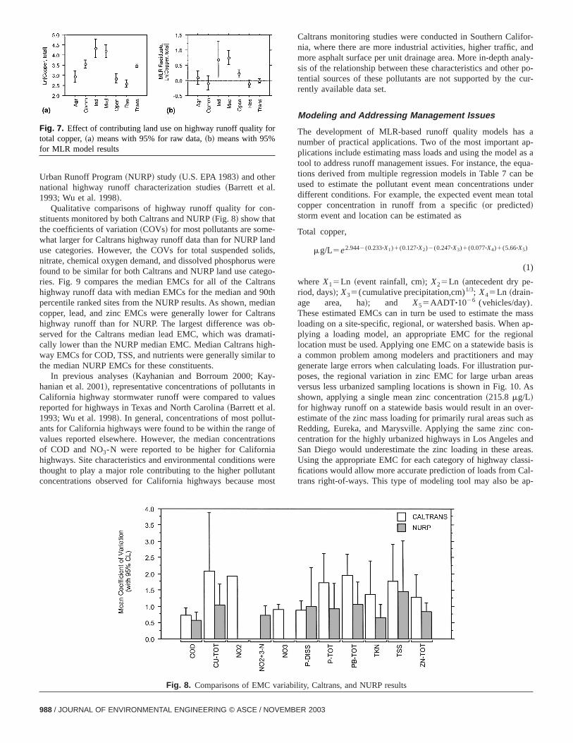
The general conclusion from these analyses is that contribing land use appears to significantly affect concentrations of mapollutants in highway runoff, but that additional data are needeto conclusively establish the specific effects for different lanuses. Although the results of analyses for the effects of land uvary by constituent, an example of a fairly typical case is illustrated in Fig. 7 for total copper concentrations in highway runofComparisons of raw data and residuals from the MLR model ftotal copper illustrate that runoff quality varies significantly fo

Fig. 6. Comparison of independent variable effects

BER 2003

Page 13

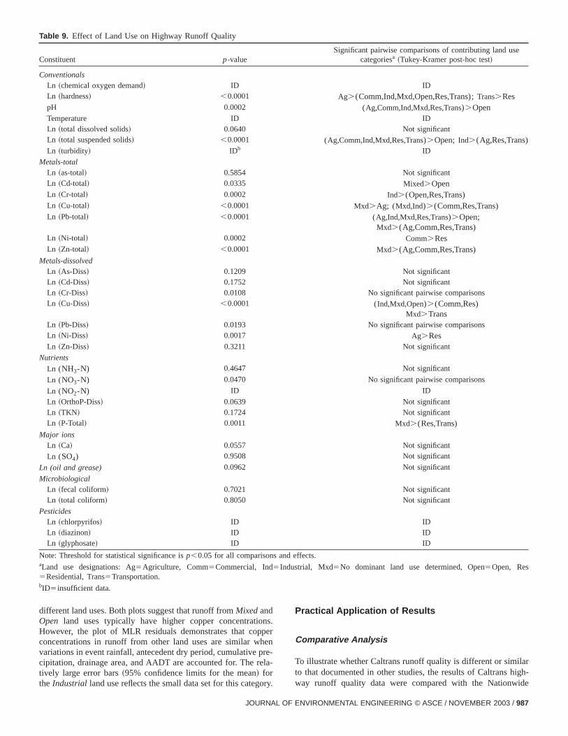
Table 9. Effect of Land Use on Highway Runoff Quality

Constituent p-valueSignificant pairwise comparisons of contributing land use

categoriesa ~Tukey-Kramer post-hoc test!

ConventionalsLn ~chemical oxygen demand! ID IDLn ~hardness! ,0.0001 Ag.(Comm,Ind,Mxd,Open,Res,Trans);Trans.RespH 0.0002 (Ag,Comm,Ind,Mxd,Res,Trans).OpenTemperature ID IDLn ~total dissolved solids! 0.0640 Not significantLn ~total suspended solids! ,0.0001 (Ag,Comm,Ind,Mxd,Res,Trans).Open; Ind.(Ag,Res,Trans)Ln ~turbidity! IDb ID

Metals-totalLn ~as-total! 0.5854 Not significantLn ~Cd-total! 0.0335 Mixed.OpenLn ~Cr-total! 0.0002 Ind.(Open,Res,Trans)Ln ~Cu-total! ,0.0001 Mxd.Ag; (Mxd,Ind).(Comm,Res,Trans)Ln ~Pb-total! ,0.0001 (Ag,Ind,Mxd,Res,Trans).Open;

Mxd.(Ag,Comm,Res,Trans)Ln ~Ni-total! 0.0002 Comm.ResLn ~Zn-total! ,0.0001 Mxd.(Ag,Comm,Res,Trans)

Metals-dissolvedLn ~As-Diss! 0.1209 Not significantLn ~Cd-Diss! 0.1752 Not significantLn ~Cr-Diss! 0.0108 No significant pairwise comparisonsLn ~Cu-Diss! ,0.0001 (Ind,Mxd,Open).(Comm,Res)

Mxd.TransLn ~Pb-Diss! 0.0193 No significant pairwise comparisonsLn ~Ni-Diss! 0.0017 Ag.ResLn ~Zn-Diss! 0.3211 Not significant

Nutrients

Ln (NH3-N) 0.4647 Not significant

Ln (NO3-N) 0.0470 No significant pairwise comparisons

Ln (NO2-N) ID ID

Ln ~OrthoP-Diss! 0.0639 Not significantLn ~TKN! 0.1724 Not significantLn ~P-Total! 0.0011 Mxd.(Res,Trans)

Major ionsLn ~Ca! 0.0557 Not significant

Ln (SO4) 0.9508 Not significant

Ln (oil and grease) 0.0962 Not significant

MicrobiologicalLn ~fecal coliform! 0.7021 Not significantLn ~total coliform! 0.8050 Not significant

PesticidesLn ~chlorpyrifos! ID IDLn ~diazinon! ID IDLn ~glyphosate! ID ID

Note: Threshold for statistical significance isp,0.05 for all comparisons and effects.aLand use designations: Ag5Agriculture, Comm5Commercial, Ind5Industrial, Mxd5No dominant land use determined, Open5Open, Res5Residential, Trans5Transportation.bID5 insufficient data.

ns.perenre-la

ry.

arigh-de

different land uses. Both plots suggest that runoff fromMixedandOpen land uses typically have higher copper concentratioHowever, the plot of MLR residuals demonstrates that copconcentrations in runoff from other land uses are similar whvariations in event rainfall, antecedent dry period, cumulative pcipitation, drainage area, and AADT are accounted for. The retively large error bars~95% confidence limits for the mean! forthe Industrial land use reflects the small data set for this catego

JOURNAL OF

-

Practical Application of Results

Comparative Analysis

To illustrate whether Caltrans runoff quality is different or similto that documented in other studies, the results of Caltrans hway runoff quality data were compared with the Nationwi

ENVIRONMENTAL ENGINEERING © ASCE / NOVEMBER 2003 / 987

Page 14

ddeo

ha

-t-o

s

t

or-ndaly-po-ur-

ap-s a

qua-bedertal

assap-al

isay

ur-asAs

r-as

n-ndas.si-l-

p-

Urban Runoff Program~NURP! study~U.S. EPA 1983! and othernational highway runoff characterization studies~Barrett et al.1993; Wu et al. 1998!.

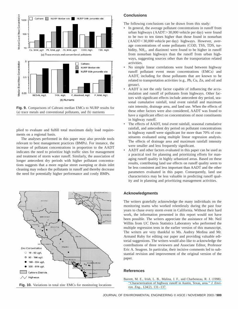
Qualitative comparisons of highway runoff quality for con-stituents monitored by both Caltrans and NURP~Fig. 8! show thatthe coefficients of variation~COVs! for most pollutants are some-what larger for Caltrans highway runoff data than for NURP lanuse categories. However, the COVs for total suspended solinitrate, chemical oxygen demand, and dissolved phosphorus wfound to be similar for both Caltrans and NURP land use categries. Fig. 9 compares the median EMCs for all of the Caltranhighway runoff data with median EMCs for the median and 90tpercentile ranked sites from the NURP results. As shown, medicopper, lead, and zinc EMCs were generally lower for Caltranhighway runoff than for NURP. The largest difference was observed for the Caltrans median lead EMC, which was dramacally lower than the NURP median EMC. Median Caltrans highway EMCs for COD, TSS, and nutrients were generally similar tthe median NURP EMCs for these constituents.

In previous analyses~Kayhanian and Borroum 2000; Kay-hanian et al. 2001!, representative concentrations of pollutants inCalifornia highway stormwater runoff were compared to valuereported for highways in Texas and North Carolina~Barrett et al.1993; Wu et al. 1998!. In general, concentrations of most pollut-ants for California highways were found to be within the range ovalues reported elsewhere. However, the median concentratioof COD and NO3-N were reported to be higher for Californiahighways. Site characteristics and environmental conditions wethought to play a major role contributing to the higher pollutanconcentrations observed for California highways because mo

Fig. 7. Effect of contributing land use on highway runoff quality fortotal copper,~a! means with 95% for raw data,~b! means with 95%for MLR model results

988 / JOURNAL OF ENVIRONMENTAL ENGINEERING © ASCE / NOVEM

s,re-

s

ns

i-

fns

re

st

Caltrans monitoring studies were conducted in Southern Califnia, where there are more industrial activities, higher traffic, amore asphalt surface per unit drainage area. More in-depth ansis of the relationship between these characteristics and othertential sources of these pollutants are not supported by the crently available data set.

Modeling and Addressing Management Issues

The development of MLR-based runoff quality models hasnumber of practical applications. Two of the most important aplications include estimating mass loads and using the model atool to address runoff management issues. For instance, the etions derived from multiple regression models in Table 7 canused to estimate the pollutant event mean concentrations undifferent conditions. For example, the expected event mean tocopper concentration in runoff from a specific~or predicted!storm event and location can be estimated as

Total copper,

mg/L5e2.9442(0.233"X1)1(0.127"X2)2(0.247"X3)1(0.077"X4)1(5.66"X5)

(1)

whereX15Ln ~event rainfall, cm!; X25Ln ~antecedent dry pe-riod, days!; X35(cumulative precipitation,cm)1/3; X45Ln ~drain-age area, ha!; and X55AADT "1026 (vehicles/day).These estimated EMCs can in turn be used to estimate the mloading on a site-specific, regional, or watershed basis. Whenplying a loading model, an appropriate EMC for the regionlocation must be used. Applying one EMC on a statewide basisa common problem among modelers and practitioners and mgenerate large errors when calculating loads. For illustration pposes, the regional variation in zinc EMC for large urban areversus less urbanized sampling locations is shown in Fig. 10.shown, applying a single mean zinc concentration~215.8mg/L!for highway runoff on a statewide basis would result in an oveestimate of the zinc mass loading for primarily rural areas suchRedding, Eureka, and Marysville. Applying the same zinc cocentration for the highly urbanized highways in Los Angeles aSan Diego would underestimate the zinc loading in these areUsing the appropriate EMC for each category of highway clasfications would allow more accurate prediction of loads from Catrans right-of-ways. This type of modeling tool may also be a

Fig. 8. Comparisons of EMC variability, Caltrans, and NURP results

BER 2003

Page 15

ls

f-

les

m

n-

-ted

y

--a-

oftots

ens-is.ty

as

setoer

usel-

eurrdeeil

pt..i-eor

b-e

r

plied to evaluate and fulfill total maximum daily load require-ments on a regional basis.

The analyses performed in this paper may also provide toorelevant to best management practices~BMPs!. For instance, theincrease of pollutant concentrations in proportion to the AADTindicates the need to prioritize high traffic sites for managemenand treatment of storm water runoff. Similarly, the association olonger antecedent dry periods with higher pollutant concentrations suggests that a more regular street sweeping or drain incleaning may reduce the pollutants in runoff and thereby decreathe need for potentially higher performance and costly BMPs.

Fig. 9. Comparisons of Caltrans median EMCs to NURP results fo~a! trace metals and conventional pollutants, and~b! nutrients

Fig. 10. Variations in total zinc EMCs for monitoring locations

JOURNAL OF

t

te

Conclusions

The following conclusions can be drawn from this study:• In general, the average pollutant concentrations in runoff fro

urban highways (AADT.30,000 vehicle per day) were foundto be two to ten times higher than those found in nonurba(AADT,30,000 vehicle per day) highways. However, average concentrations of some pollutants~COD, TSS, TDS, tur-bidity, NH3 , and diazinon! were found to be higher in runofffrom nonurban highways than the runoff from urban highways, suggesting sources other than the transportation relaactivities.

• No simple linear correlations were found between highwarunoff pollutant event mean concentrations~EMCs! andAADT, including for those pollutants that are known to berelated to transportation activities~e.g., Pb, Cu, Zn, and oil andgrease!.

• AADT is not the only factor capable of influencing the accumulation and runoff of pollutants from highways. Other factors with significant effects include antecedent dry period, sesonal cumulative rainfall, total event rainfall and maximumrain intensity, drainage area, and land use. When the effectsthese other factors were also considered, AADT was foundhave a significant effect on concentrations of most constituenin highway runoff.

• The effects of AADT, total event rainfall, seasonal cumulativrainfall, and antecedent dry period on pollutant concentratioin highway runoff were significant for more than 70% of constituents evaluated using multiple linear regression analysThe effects of drainage area and maximum rainfall intensiwere smaller and less frequently significant.

• AADT and other factors evaluated in this paper can be useda practical tool for planning and prioritizing efforts for man-aging runoff quality in highly urbanized areas. Based on theresults, contributing land use effects on runoff quality seembe less consistent and less important than AADT and the othparameters evaluated in this paper. Consequently, landcharacteristics may be less valuable in predicting runoff quaity and in planning and prioritizing management activities.

Acknowledgments

The writers gratefully acknowledge the many individuals on thmonitoring teams who worked relentlessly during the past foyears to chase every storm event in California. Without their hawork, the information presented in this report would not havbeen possible. The writers appreciate the assistance of Mr. NWillits from UC Davis Statistics Laboratory who performed themultiple regression tests in the earlier version of this manuscriThe writers are very thankful to Ms. Audrey Medina and MrArmand Ruby for editing our paper and providing valuable edtorial suggestions. The writers would also like to acknowledge thcontributions of three reviewers and Associate Editor, ProfessEric A. Seagren. In particular, their incisive comments led to sustantial revision and improvement of the original version of thpaper.

References

Barrett, M. E., Irish, L. B., Malina, J. F., and Charbeneau, R. J.~1998!.‘‘Characterization of highway runoff in Austin, Texas, area.’’J. Envi-ron. Eng.,124~2!, 131–137.

ENVIRONMENTAL ENGINEERING © ASCE / NOVEMBER 2003 / 989

Page 16

d

l-es

II:

um

he

n

n

e-

r

nd

h-

r

California Department of Transportation~Caltrans!. ~2000a!. Guidancemanual: Stormwater monitoring protocols, 2nd Ed., California Dept.of Transportation, Sacramento, Calif.,Rep. No. CTSW-RT-00-005.

Caltrans~2000b!. Data reporting protocols, 2nd Ed., California Dept. ofTransportation, Sacramento, Calif.,Rep. No. CTSW-RT-00-002.

Chui, T. W., Mar, B. W., and Horner, R. R.~1982!. ‘‘Pollutant loadingmodel for highway runoff.’’J. Environ. Eng.,108~6!, 1193–1210.

D’Agostino, R.~1971!. ‘‘An omnibus test of normality for moderate anlarge samples.’’Biometrika,58, 341–348.

Dorman, M. E.~1988!. ‘‘Retention, detention, and overland flow for polutant removal from highway stormwater runoff: Interim guidelinfor management measures.’’U.S. Dept. of Transportation, Washing-ton, D.C.

Driscoll, E. D., Shelley, P. E., and Strecker, E. W.~1990!. ‘‘Pollutantloadings and impacts from highway stormwater runoff volume IAnalytical investigation and research report.’’Publication No. FHWA-RD-88-008, Federal Highway Administration, Washington, D.C.

Gupta, M. K., Agnew, R. W., and Kobriger, N. P.~1981!. ‘‘Constituents ofhighway runoff Vol. 1 state-of-the-art report.’’Rep. No. FHWA/RD-81/042, Federal Highway Administration, Washington, D.C.

Helsel, D., and Cohn, T.~1988!. ‘‘Estimation of descriptive statistics formultiply censored water quality data.’’Water Resour. Res.,24~12!,1997–2004.

Irish, L. B. Jr., Malina, J. F., Charbeneau, R. J., and Ward, G. H.~1995!.‘‘Solids loading model for an urban highway.’’Proc., 1st Int. Conf. onWater Resources, Part 2. San Antonio, Tex.

Kayhanian, M., and Borroum, S.~2000!. ‘‘Characterization of the high-way stormwater runoff in California.’’Proc., 72nd Annual Conf. onCalifornia Water Environmental Association, Sacramento, Calif.,April 16–19.

Kayhanian, M., Johnston, M., Johnston, J., Yamaguchi, H., and BorroB. ~2001!. ‘‘Caltrans storm water management program.’’Stormwater,2~2!, 52–67.

Kerri, K. D., Racin, J. A., and Howell, R. B.~1985!. ‘‘Forecasting pol-lutant loads from highway runoff.’’Transp. Res. Rec.,1017, 39–46.

Kim, N. D., and Fregusson, J. E.~1994!. ‘‘The concentrations, distribu-tion and sources of cadmium, copper, lead, and zinc in the atmospof an urban environment.’’Sci. Total Environ.,144, 179–189.

990 / JOURNAL OF ENVIRONMENTAL ENGINEERING © ASCE / NOVEM

,

re

Kobriger, N. K., and Gainopolos, A.~1984!. ‘‘Sources and migration ofhighway runoff pollutants volume III: research report.’’PublicationNo. FHWA/RD-84/059, Federal Highway Administration, Washing-ton, D.C.

Laxen, D. P. H., and Harrison, R. M.~1977!. ‘‘Highway as a source ofwater pollution: an appraisal with the heavy metal lead.’’Water Res.,11~1!, 1–11.

Mckenzie, D. J., and Miller, T. L.~1983!. ‘‘Water-quality assessment ofstormwater runoff from a heavily used urban highway bridge iMiami, Florida.’’ Report No. 83-4153, USGS, Water Resources Inves-tigations, Menlo Park, Calif.

Moe, R. D., Bullin, J. A., and Lougheed, M. J.~1982!. ‘‘Atmosphericparticulate analysis and impact of highway runoff on water quality iTexas.’’Report No. 191-IF, Texas State Department of Highways andPublic Transportation.

Ryan, T., and Joiner, B.~1976!. ‘‘Normal probability plots and tests fornormality.’’ White paper, Statistics Dept., The Pennsylvania StateUniv., Univ. Park, Pa.

Shapiro, S., and Wilk, M.~1968!. ‘‘The joint assessment of normality ofseveral independent samples.’’Technometrics,10, 825–839.

Shumway, R. H., Azari, A. S., and Kayhanian, M.~2002! ‘‘Statisticalapproaches to estimating mean water quality concentrations with dtection limits.’’ Environ. Sci. Technol., 36~15!, 3345–3353.

Stotz, G. ~1987!. ‘‘Investigation of the properties of the surface waterunoff from federal highways in the FGR.’’Sci. Total Environ.,59,329–337.

U.S. Environmental Protection Agency~U.S. EPA! ~1983!. ‘‘Results ofthe nationwide urban runoff program—Vol. 1—Final report.’’PB84–185552, U.S. Environmental Protection Agency, Washington, D.C.

Wistrom, A. O., and Matsumoto, M. R.~1999!. ‘‘Highway runoff: Con-taminant sources and deposition mechanisms.’’ Dept. of Chemical aEnvironmental Engineering, Univ. of California, Riverside, Calif.

Wu, S. J., Allan, C. J., Saunders, W. L., and Evett, J. B.~1998!. ‘‘Char-acterization and pollutant loading estimation for urban and rural higway runoff.’’ J. Environ. Eng.,124~7!, 584–592.

Young, G.~1996!. ‘‘Evaluation and management of highway runoff watequality.’’ Federal Highway Administration, Washington, D.C.

BER 2003