Purdue University Purdue e-Pubs Open Access Dissertations eses and Dissertations Fall 2014 Image analysis using visual saliency with applications in hazmat sign detection and recognition Bin Zhao Purdue University Follow this and additional works at: hps://docs.lib.purdue.edu/open_access_dissertations Part of the Computer Engineering Commons , Computer Sciences Commons , and the Electrical and Electronics Commons is document has been made available through Purdue e-Pubs, a service of the Purdue University Libraries. Please contact [email protected] for additional information. Recommended Citation Zhao, Bin, "Image analysis using visual saliency with applications in hazmat sign detection and recognition" (2014). Open Access Dissertations. 401. hps://docs.lib.purdue.edu/open_access_dissertations/401

Welcome message from author
This document is posted to help you gain knowledge. Please leave a comment to let me know what you think about it! Share it to your friends and learn new things together.
Transcript
Purdue UniversityPurdue e-Pubs
Open Access Dissertations Theses and Dissertations
Fall 2014
Image analysis using visual saliency withapplications in hazmat sign detection andrecognitionBin ZhaoPurdue University
Follow this and additional works at: https://docs.lib.purdue.edu/open_access_dissertations
Part of the Computer Engineering Commons, Computer Sciences Commons, and the Electricaland Electronics Commons
This document has been made available through Purdue e-Pubs, a service of the Purdue University Libraries. Please contact [email protected] foradditional information.
Recommended CitationZhao, Bin, "Image analysis using visual saliency with applications in hazmat sign detection and recognition" (2014). Open AccessDissertations. 401.https://docs.lib.purdue.edu/open_access_dissertations/401

Graduate School ETD Form 9 (Revised 12/07)
PURDUE UNIVERSITY GRADUATE SCHOOL
Thesis/Dissertation Acceptance
This is to certify that the thesis/dissertation prepared
By
Entitled
For the degree of
Is approved by the final examining committee:
Chair
To the best of my knowledge and as understood by the student in the Research Integrity and Copyright Disclaimer (Graduate School Form 20), this thesis/dissertation adheres to the provisions of Purdue University’s “Policy on Integrity in Research” and the use of copyrighted material.
Approved by Major Professor(s): ____________________________________
____________________________________
Approved by: Head of the Graduate Program Date
Bin Zhao
Image Analysis Using Visual Saliency with Applications in Hazmat Sign Detection and Recognition
Doctor of Philosophy
EDWARD J. DELP
ARIF GHAFOOR
CHIH-CHUN WANG
JAN P. ALLEBACH
EDWARD J. DELP
V. Balakrishnan 10-15-2014


IMAGE ANALYSIS USING VISUAL SALIENCY WITH APPLICATIONS
IN HAZMAT SIGN DETECTION AND RECOGNITION
A Dissertation
Submitted to the Faculty
of
Purdue University
by
Bin Zhao
In Partial Fulfillment of the
Requirements for the Degree
of
Doctor of Philosophy
December 2014
Purdue University
West Lafayette, Indiana

ii
To my parents and my grandparents,
for their endless love, support, and encouragement

iii
ACKNOWLEDGMENTS
I would not have been the person I am today without the support and guidance
of my advisor, Professor Edward J. Delp. This dissertation would not have been
possible without the encouragement and insights from my advisor. I especially thank
him for teaching me how to learn, how to think, and how to collaborate. He has been
my best mentor and what he has taught me all these years is the enduring treasure
of my life.
I especially thank my advisory committee members: Professor Jan P. Allebach,
Professor Arif Ghafoor, and Professor Chih-Chun Wang for their inspired teaching,
support, and encouragement.
I want to thank Dr. Albert Parra, Joonsoo Kim, and He Li for their great collabo-
ration and contribution to the Mobile Emergency Response GuidE (MERGE) project,
for providing constructive feedback to my research and for always being willing to
support my work.
I want to extend my thanks to all my former and current colleagues in the Video
and Image Processing Laboratory (VIPER). I thank all my brilliant colleagues: Dr.
Aravind Mikkilineni, Dr. Kevin Lorenz, Dr. Nitin Khanna, Dr. Satyam Srivastava,
Dr. Ka Ki Ng, Dr. Fengqing Maggie Zhu, Dr. Marc Bosch Ruiz, Dr. Meilin Yang,
Dr. Ye He, Dr. Chang Xu, Dr. Albert Parra, Ziad Ahmad, Jeehyun Choe, Neeraj
Gadgil, Deen King-Smith, Joonsoo Kim, Soonam Lee, He Li, Khalid Tahboub, and
Yu Wang. I also thank the visiting students in the VIPER lab: Blanca Delgado, Javi
Ribera, Thitiporn Pramoun and Kharittha Thongkor. I thank all my friends in the
VIPER lab for all the help they have given and all the joy they have brought.
I want to deeply appreciate my parents and my grandparents for their endless
love, support, and encouragement. They have given me more than I could imagine in
my life.
iv
I gratefully thank the School of Electrical and Computer Engineering of Purdue
University for accepting me into the Doctoral program and providing such a memo-
rable environment to do research.
The hazardous material sign images shown in this thesis were partially obtained
in cooperation with the officers in the U.S. Transportation Security Administration
(TSA). I gratefully acknowledge their cooperation in the Mobile Emergency Response
GuidE (MERGE) project.
This dissertation was supported by the Visual Analytics for Command, Control,
and Interoperability Environments (VACCINE) Center of the U.S. Department of
Homeland Security (DHS) under Award Number 2009-ST-061-CI000. I gratefully
thank the VACCINE Center for the sponsorship of the MERGE research project in
this dissertation.

v
TABLE OF CONTENTS
Page
LIST OF TABLES . . . . . . . . . . . . . . . . . . . . . . . . . . . . . . . . ix
LIST OF FIGURES . . . . . . . . . . . . . . . . . . . . . . . . . . . . . . . xi
ABSTRACT . . . . . . . . . . . . . . . . . . . . . . . . . . . . . . . . . . . xv
1 INTRODUCTION . . . . . . . . . . . . . . . . . . . . . . . . . . . . . . 1
1.1 Problem Statement . . . . . . . . . . . . . . . . . . . . . . . . . . . 1
1.2 Visual Saliency . . . . . . . . . . . . . . . . . . . . . . . . . . . . . 1
1.3 Hazmat Sign Detection and Recognition . . . . . . . . . . . . . . . 3
1.4 Error Concealment for Scalable Video Coding . . . . . . . . . . . . 4
1.5 Contributions of This Thesis . . . . . . . . . . . . . . . . . . . . . . 5
1.6 Publications Resulting from This Thesis . . . . . . . . . . . . . . . 7
2 VISUAL SALIENCY MODELS INTHE FREQUENCY DOMAIN . . . . . . . . . . . . . . . . . . . . . . . 9
2.1 Visual Saliency . . . . . . . . . . . . . . . . . . . . . . . . . . . . . 9
2.2 Visual Saliency Model Families . . . . . . . . . . . . . . . . . . . . 11
2.2.1 Separate Visual Saliency Model Family . . . . . . . . . . . . 13
2.2.2 Composite Visual Saliency Model Family . . . . . . . . . . . 13
2.2.3 Connections Between Visual Saliency Model Families and EarlyHuman Visual System . . . . . . . . . . . . . . . . . . . . . 14
2.2.4 Color Spaces . . . . . . . . . . . . . . . . . . . . . . . . . . 17
2.2.5 Quaternion Representation . . . . . . . . . . . . . . . . . . . 19
2.3 Proposed Visual Saliency Models . . . . . . . . . . . . . . . . . . . 23
2.3.1 Spectral Analysis Approaches . . . . . . . . . . . . . . . . . 23
2.3.2 Entropy-Based Saliency Map Selection . . . . . . . . . . . . 26
2.3.3 Post-Processing . . . . . . . . . . . . . . . . . . . . . . . . . 27
vi
Page
2.3.4 Visual Saliency Model Using Gamma Corrected Spectrum (GCS) 27
2.3.5 Visual Saliency Model Using Gamma Corrected Log Spectrum(GCLS) . . . . . . . . . . . . . . . . . . . . . . . . . . . . . 29
2.3.6 Visual Saliency Model Using Low-Pass Filtered Spectrum (LPFS) 29
2.3.7 Visual Saliency Model Using Low-Pass Filtered Log Spectrum(LPFLS) . . . . . . . . . . . . . . . . . . . . . . . . . . . . . 31
2.3.8 Visual Saliency Model Using Gaussian Filtered Spectrum (GFS) 31
2.3.9 Visual Saliency Model Using Gaussian Filtered Log Spectrum(GFLS) . . . . . . . . . . . . . . . . . . . . . . . . . . . . . 32
2.3.10 Naming Convention of the Extended Models . . . . . . . . . 32
2.3.11 Visual Saliency Model Evaluation . . . . . . . . . . . . . . . 33
2.3.12 Parameter Issues . . . . . . . . . . . . . . . . . . . . . . . . 37
2.4 Experimental Results . . . . . . . . . . . . . . . . . . . . . . . . . . 40
2.4.1 Predicting Eye Fixation . . . . . . . . . . . . . . . . . . . . 40
3 HAZMAT SIGN DETECTION AND RECOGNITIONUSING VISUAL SALIENCY . . . . . . . . . . . . . . . . . . . . . . . . 65
3.1 Review of Existing Sign Detection and Recognition Methods . . . . 66
3.1.1 Sign Location Detection . . . . . . . . . . . . . . . . . . . . 66
3.1.2 Sign Recognition . . . . . . . . . . . . . . . . . . . . . . . . 68
3.1.3 Shape Descriptors . . . . . . . . . . . . . . . . . . . . . . . . 69
3.2 Review of Existing Hazmat Sign Detection and Recognition Systems 70
3.2.1 Hazmat Sign Detection Based on SURF and HBP . . . . . . 70
3.2.2 Hazmat Sign Detection Based on HOG . . . . . . . . . . . . 72
3.2.3 Comparison to MERGE . . . . . . . . . . . . . . . . . . . . 72
3.3 Proposed Hazmat Sign Detection and Recognition System . . . . . 74
3.3.1 MERGE System Overview . . . . . . . . . . . . . . . . . . . 74
3.4 Hazmat Sign Detection and Recognition Method 1 . . . . . . . . . . 78
3.4.1 Saliency Map Generation . . . . . . . . . . . . . . . . . . . . 79
3.4.2 Salient Region Extraction . . . . . . . . . . . . . . . . . . . 79
vii
Page
3.4.3 Convex Quadrilateral Shape Detection . . . . . . . . . . . . 80
3.4.4 Duplicate Sign Removal . . . . . . . . . . . . . . . . . . . . 80
3.4.5 Color Recognition . . . . . . . . . . . . . . . . . . . . . . . . 81
3.5 Hazmat Sign Detection and Recognition Method 2 . . . . . . . . . . 82
3.5.1 Saliency Map Generation . . . . . . . . . . . . . . . . . . . . 83
3.5.2 Salient Region Extraction . . . . . . . . . . . . . . . . . . . 85
3.5.3 Contour Extraction . . . . . . . . . . . . . . . . . . . . . . . 85
3.5.4 Fourier Descriptor Generation . . . . . . . . . . . . . . . . . 90
3.5.5 Correlation-Based Contour Matching . . . . . . . . . . . . . 91
3.5.6 Duplicate Sign Removal . . . . . . . . . . . . . . . . . . . . 93
3.5.7 Color Recognition . . . . . . . . . . . . . . . . . . . . . . . . 95
3.6 Experimental Results . . . . . . . . . . . . . . . . . . . . . . . . . . 102
3.6.1 Image Datasets . . . . . . . . . . . . . . . . . . . . . . . . . 102
3.6.2 The First Experiment . . . . . . . . . . . . . . . . . . . . . 109
3.6.3 The Second Experiment . . . . . . . . . . . . . . . . . . . . 118
4 ERROR CONCEALMENT FORSCALABLE VIDEO CODING . . . . . . . . . . . . . . . . . . . . . . . . 129
4.1 Error Concealment Methods . . . . . . . . . . . . . . . . . . . . . . 131
4.1.1 Conventional Error Concealment Methods . . . . . . . . . . 131
4.1.2 Related Work . . . . . . . . . . . . . . . . . . . . . . . . . . 131
4.1.3 Proposed Error Concealment Methods . . . . . . . . . . . . 133
4.2 System Implementation . . . . . . . . . . . . . . . . . . . . . . . . . 138
4.3 Experimental Results . . . . . . . . . . . . . . . . . . . . . . . . . . 140
5 CONCLUSIONS AND FUTURE WORK . . . . . . . . . . . . . . . . . . 148
5.1 Conclusions . . . . . . . . . . . . . . . . . . . . . . . . . . . . . . . 148
5.2 Future Work . . . . . . . . . . . . . . . . . . . . . . . . . . . . . . . 150
5.3 Publications Resulting from This Work . . . . . . . . . . . . . . . . 151
LIST OF REFERENCES . . . . . . . . . . . . . . . . . . . . . . . . . . . . 153

viii
Page
A MERGE IMAGE ACQUISITION PROTOCOL . . . . . . . . . . . . . . 164
VITA . . . . . . . . . . . . . . . . . . . . . . . . . . . . . . . . . . . . . . . 172

ix
LIST OF TABLES
Table Page
2.1 The rank of extended GCS models, the maximum sAUC score, and theassociated Gaussian σopt (in image largest dimension). . . . . . . . . . . 46
2.2 The rank of extended GCLS models, the maximum sAUC score, and theassociated Gaussian σopt (in image largest dimension). . . . . . . . . . . 46
2.3 The rank of extended LPFS models, the maximum sAUC score, and theassociated Gaussian σopt (in image largest dimension). . . . . . . . . . . 47
2.4 The rank of extended LPFLS models, the maximum sAUC score, and theassociated Gaussian σopt (in image largest dimension). . . . . . . . . . . 47
2.5 The rank of extended GFS models, the maximum sAUC score, and theassociated Gaussian σopt (in image largest dimension). . . . . . . . . . . 48
2.6 The rank of extended GFLS models, the maximum sAUC score, and theassociated Gaussian σopt (in image largest dimension). . . . . . . . . . . 48
2.7 The summary of the best extended models: The rank in the same modelgroup, the maximum sAUC score, and the associated Gaussian σopt (inimage largest dimension). . . . . . . . . . . . . . . . . . . . . . . . . . 49
2.8 The rank of each saliency model, the maximum sAUC score, and theassociated Gaussian σopt (in image largest dimension). . . . . . . . . . . 62
3.1 Thresholds and parameters used in our proposed method. Automaticallydetermined ones are denoted by *. . . . . . . . . . . . . . . . . . . . . 88
3.2 The color look-up table based on the 32 uniform distributed hue segments. 96
3.3 The relation among the image resolution, the distance from a camera toa hazmat sign, and the number of pixels on a hazmat sign in the thirdimage dataset (Dataset-3) with comparison to a typical STOP sign. . . 108
3.4 Average execution time (in seconds), distribution and score of the saliencymodels (color spaces) in the first image dataset (Dataset-1). . . . . . . 111
3.5 The pixel usage and sign coverage in the extracted salient regions for thethree image datasets. . . . . . . . . . . . . . . . . . . . . . . . . . . . . 119
3.6 Image analysis results for the first image dataset (Dataset-1). . . . . . 121

x
Table Page
3.7 Image analysis results for the second image dataset (Dataset-2). . . . . 122
3.8 Image analysis results of Method 1 using four saliency maps for the thirdimage dataset (Dataset-3). . . . . . . . . . . . . . . . . . . . . . . . . . 124
3.9 Image analysis results of Method 2 without using saliency maps for thethird image dataset (Dataset-3). . . . . . . . . . . . . . . . . . . . . . . 125
3.10 Image analysis results of Method 2 using two saliency maps for the thirdimage dataset (Dataset-3). . . . . . . . . . . . . . . . . . . . . . . . . . 126
4.1 Average Decoding Time per Frame of the Existing and Proposed ErrorConcealment Methods (in Milliseconds) . . . . . . . . . . . . . . . . . . 141

xi
LIST OF FIGURES
Figure Page
1.1 Example of hazmat signs. . . . . . . . . . . . . . . . . . . . . . . . . . 4
2.1 The generalization of visual saliency models in the frequency domain. . 12
2.2 Two visual saliency model families in the frequency domain. . . . . . . 12
2.3 The primary visual pathway of the human visual system and the three keycomponents. . . . . . . . . . . . . . . . . . . . . . . . . . . . . . . . . . 16
2.4 Examples of phase spectrum contains important visual saliency informa-tion. Reproduced from [30] . . . . . . . . . . . . . . . . . . . . . . . . 24
2.5 An example of amplitude spectrum contains both saliency and non-saliencyinformation. Reproduced from [35] . . . . . . . . . . . . . . . . . . . . 24
2.6 The classification of true positive, false positive, true negative, and falsenegative. . . . . . . . . . . . . . . . . . . . . . . . . . . . . . . . . . . . 36
2.7 An example of some prerequisites for computing sAUC score. (A) Thegenerated saliency map on a certain image, (B) The binarized saliencymap thresholded at 0.5, (C) The positive sample set of eye fixation pointsonly on this image (Gaussian blurred heat map representation), (D) Thenegative sample set of eye fixation points containing all fixation pointsacross the entire image dataset but excluding those points in the posi-tive sample set (Gaussian blurred heat map representation). Reproducedfrom [33] . . . . . . . . . . . . . . . . . . . . . . . . . . . . . . . . . . . 38
2.8 An example of the shuffled ROC used for computing the sAUC score (truepositive rate (TPR) versus false positive rate (FPR)). Reproduced from [33] 39
2.9 The sAUC score of each FT-based model in the separate model family(BT dataset). . . . . . . . . . . . . . . . . . . . . . . . . . . . . . . . . 42
2.10 The sAUC score of each HFT-based model in the composite model family(BT dataset). . . . . . . . . . . . . . . . . . . . . . . . . . . . . . . . . 43
2.11 The sAUC score of each FT-based model in the separate model family (Lidataset). . . . . . . . . . . . . . . . . . . . . . . . . . . . . . . . . . . . 44
2.12 The sAUC score of each HFT-based model in the composite model family(Li dataset). . . . . . . . . . . . . . . . . . . . . . . . . . . . . . . . . . 45
xii
Figure Page
2.13 The sAUC score of each model (BT dataset). . . . . . . . . . . . . . . 51
2.14 The average execution time of each model (BT dataset). . . . . . . . . 52
2.15 The sAUC score of each model (Li dataset). . . . . . . . . . . . . . . . 53
2.16 The average execution time of each model (Li dataset). . . . . . . . . . 54
2.17 Examples of saliency maps from different models for two images (BTdataset). . . . . . . . . . . . . . . . . . . . . . . . . . . . . . . . . . . . 55
2.18 Examples of saliency maps from different models for two images (BTdataset). . . . . . . . . . . . . . . . . . . . . . . . . . . . . . . . . . . . 56
2.19 Examples of saliency maps from different models for two images (BTdataset). . . . . . . . . . . . . . . . . . . . . . . . . . . . . . . . . . . . 57
2.20 Examples of saliency maps from different models for two images (Li dataset). 58
2.21 Examples of saliency maps from different models for two images (Li dataset). 59
2.22 Examples of saliency maps from different models for two images (Li dataset). 60
2.23 The distribution of eye fixation of all the images in BT dataset (left) andLi dataset (right). . . . . . . . . . . . . . . . . . . . . . . . . . . . . . . 64
2.24 The Gaussian blurred heat map representation of eye fixation of all theimages in BT dataset (left) and Li dataset (right), where the Gaussianσ = 0.005 (in image largest dimension). . . . . . . . . . . . . . . . . . . 64
3.1 Examples of two hazmat signs divided into three separate parts. . . . . 65
3.2 Hazmat sign location detection and content recognition system. . . . . 75
3.3 Manually search hazmat signs by UN identifier numbers, template images,symbols, and classes. . . . . . . . . . . . . . . . . . . . . . . . . . . . . 76
3.4 Mobile application user interface at each step. . . . . . . . . . . . . . . 77
3.5 Proposed hazmat sign detection and recognition method 1. . . . . . . . 78
3.6 Examples of image analysis. . . . . . . . . . . . . . . . . . . . . . . . . 81
3.7 A diamond shaped binary image represents the shape template of a hazmatsign. . . . . . . . . . . . . . . . . . . . . . . . . . . . . . . . . . . . . . 83
3.8 Proposed hazmat sign detection and recognition method 2. . . . . . . . 84
3.9 Example of image binarization using the proposed adaptive thresholdingmethod comparing with using Ostu’s method. . . . . . . . . . . . . . . 89
xiii
Figure Page
3.10 The the shape variations of using the first 4, 8, 16, 32, 50 and 100 ACFourier coefficients. . . . . . . . . . . . . . . . . . . . . . . . . . . . . . 92
3.11 Comparison of the contours of some shapes and their matching costs e. 94
3.12 Hazmat sign detection and recognition system. . . . . . . . . . . . . . . 95
3.13 Examples of the proposed color recognition method for two white hazmatsigns at 50 feet. . . . . . . . . . . . . . . . . . . . . . . . . . . . . . . . 98
3.14 Examples of the proposed color recognition method for two red hazmatsigns at 50 feet. . . . . . . . . . . . . . . . . . . . . . . . . . . . . . . . 99
3.15 Examples of the proposed color recognition method for orange and yellowhazmat signs at 50 feet. . . . . . . . . . . . . . . . . . . . . . . . . . . 100
3.16 Examples of the proposed color recognition method for green and bluehazmat signs at 50 feet. . . . . . . . . . . . . . . . . . . . . . . . . . . 101
3.17 Examples of the first image dataset (Dataset-1) in different conditions(left to right then top to bottom): low resolution, perspective distortion;blurred sign, shaded sign. . . . . . . . . . . . . . . . . . . . . . . . . . 103
3.18 Examples of the second image dataset (Dataset-2) in different conditions(left to right then top to bottom): low resolution, perspective distortion;blurred sign, shaded sign. . . . . . . . . . . . . . . . . . . . . . . . . . 104
3.19 Examples of the 6 signs of Dataset-3 at 10 feet in portrait mode (left toright then top to bottom): red sign, green sign, blue sign; orange sign,yellow sign, white sign. . . . . . . . . . . . . . . . . . . . . . . . . . . . 105
3.20 Examples of the 6 signs of Dataset-3 at 10 feet in landscape mode (leftto right then top to bottom): red sign, green sign, blue sign; orange sign,yellow sign, white sign. . . . . . . . . . . . . . . . . . . . . . . . . . . . 106
3.21 Examples of bounding box images for a typical STOP sign and a hazmatsign at the same distance 25, 50, 100, and 150 feet. . . . . . . . . . . . 107
3.22 An example of good saliency map with the four types of salient regions(top to bottom then left to right): original image, good saliency map;high salient regions, middle salient regions; low salient regions, non-salientregions. . . . . . . . . . . . . . . . . . . . . . . . . . . . . . . . . . . . 112
3.23 An example of fair saliency map with the four types of salient regions (topto bottom then left to right): original image, fair saliency map; high salientregions, middle salient regions; low salient regions, non-salient regions. 113
xiv
Figure Page
3.24 An example of bad saliency map with the four types of salient regions (topto bottom then left to right): original image, bad saliency map; high salientregions, middle salient regions; low salient regions, non-salient regions. 114
3.25 An example of lost saliency map with the four types of salient regions (topto bottom then left to right): original image, lost saliency map; high salientregions, middle salient regions; low salient regions, non-salient regions. 115
3.26 Examples of saliency maps from different methods for two hazmat signimages in portrait mode. . . . . . . . . . . . . . . . . . . . . . . . . . . 116
3.27 Examples of saliency maps from different methods for two hazmat signimages in landscape mode. . . . . . . . . . . . . . . . . . . . . . . . . . 117
4.1 The proposed inter-layer motion vector averaging approach using adap-tively averaging over multiple types of motion vectors in two layers. . . 134
4.2 Optimum index matrixes of different size. . . . . . . . . . . . . . . . . 136
4.3 The proposed slice interleaving scheme in a GOP (8 frames). . . . . . . 137
4.4 Y-PSNR of the Football BL & EL frames (BPLR=10%). . . . . . . . . 142
4.5 Y-PSNR of the Football BL & EL frames (BPLR=20%). . . . . . . . . 143
4.6 Rate-Distortion of the Bus sequence (BPLR=10%, 20%). . . . . . . . . 145
4.7 Rate-Distortion of the Football sequence (BPLR=10%, 20%). . . . . . . 146
4.8 Rate-Distortion of the Foreman sequence (BPLR=10%, 20%). . . . . . 147
A.1 Top view of the setup environment. . . . . . . . . . . . . . . . . . . . . 168
A.2 Image recording form for the MERGE project. . . . . . . . . . . . . . . 169
A.3 Hazmat sign identifiers. . . . . . . . . . . . . . . . . . . . . . . . . . . 170
A.4 Examples and screenshots of the two cases of image analysis results, haz-mat sign found (left) and not found (right). . . . . . . . . . . . . . . . 170
A.5 Examples of completed image recording form for hazmat sign found inFigure A.4 (left). . . . . . . . . . . . . . . . . . . . . . . . . . . . . . . 171
A.6 Examples of completed image recording form for hazmat sign not foundin Figure A.4 (right). . . . . . . . . . . . . . . . . . . . . . . . . . . . . 171

xv
ABSTRACT
Zhao, Bin Ph.D., Purdue University, December 2014. Image Analysis Using VisualSaliency with Applications in Hazmat Sign Detection and Recognition. MajorProfessor: Edward J. Delp.
Visual saliency is the perceptual process that makes attractive objects “stand
out” from their surroundings in the low-level human visual system. Visual saliency
has been modeled as a preprocessing step of the human visual system for selecting
the important visual information from a scene. We investigate bottom-up visual
saliency using spectral analysis approaches. We present separate and composite model
families that generalize existing frequency domain visual saliency models. We propose
several frequency domain visual saliency models to generate saliency maps using new
spectrum processing methods and an entropy-based saliency map selection approach.
A group of saliency map candidates are then obtained by inverse transform. A final
saliency map is selected among the candidates by minimizing the entropy of the
saliency map candidates. The proposed models based on the separate and composite
model families are also extended to various color spaces. We develop an evaluation
tool for benchmarking visual saliency models. Experimental results show that the
proposed models are more accurate and efficient than most state-of-the-art visual
saliency models in predicting eye fixation.
We use the above visual saliency models to detect the location of hazardous ma-
terial (hazmat) signs in complex scenes. We develop a hazmat sign location detection
and content recognition system using visual saliency. Saliency maps are employed to
extract salient regions that are likely to contain hazmat sign candidates and then use
a Fourier descriptor based contour matching method to locate the border of hazmat
signs in these regions. This visual saliency based approach is able to increase the

xvi
accuracy of sign location detection, reduce the number of false positive objects, and
speed up the overall image analysis process. We also propose a color recognition
method to interpret the color inside the detected hazmat sign. Experimental results
show that our proposed hazmat sign location detection method is capable of detect-
ing and recognizing projective distorted, blurred, and shaded hazmat signs at various
distances.
In other work we investigate error concealment for scalable video coding (SVC).
When video compressed with SVC is transmitted over loss-prone networks, the de-
compressed video can suffer severe visual degradation across multiple frames. In order
to enhance the visual quality, we propose an inter-layer error concealment method us-
ing motion vector averaging and slice interleaving to deal with burst packet losses and
error propagation. Experimental results show that the proposed error concealment
methods outperform two existing methods.
1
1. INTRODUCTION
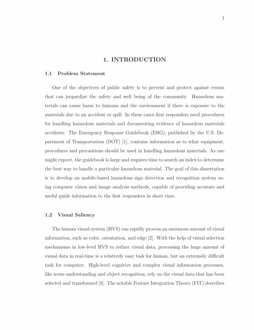
1.1 Problem Statement
One of the objectives of public safety is to prevent and protect against events
that can jeopardize the safety and well being of the community. Hazardous ma-
terials can cause harm to humans and the environment if there is exposure to the
materials due to an accident or spill. In these cases first responders need procedures
for handling hazardous materials and documenting evidence of hazardous materials
accidents. The Emergency Response Guidebook (ERG), published by the U.S. De-
partment of Transportation (DOT) [1], contains information as to what equipment,
procedures and precautions should be used in handling hazardous materials. As one
might expect, the guidebook is large and requires time to search an index to determine
the best way to handle a particular hazardous material. The goal of this dissertation
is to develop an mobile-based hazardous sign detection and recognition system us-
ing computer vision and image analysis methods, capable of providing accurate and
useful guide information to the first responders in short time.
1.2 Visual Saliency
The human visual system (HVS) can rapidly process an enormous amount of visual
information, such as color, orientation, and edge [2]. With the help of visual selection
mechanisms in low-level HVS to reduce visual data, processing the large amount of
visual data in real-time is a relatively easy task for human, but an extremely difficult
task for computer. High-level cognitive and complex visual information processes,
like scene understanding and object recognition, rely on the visual data that has been
selected and transformed [3]. The notable Feature Integration Theory (FIT) describes

2
visual attention as having two phases [4]. In the pre-attentive phase, the early vision
system can rapidly process an enormous amount of low-level visual features in parallel,
such as color, motion and edges [4]. Distinctive features (e.g., luminous color, high
velocity motion) will “stand out” automatically in the pre-attentive stage and then
the salient regions draw more attention. In the next phase, the visual cortex performs
more complex operations, such as object detection, tracking, recognition [5, 6].
There are close relations but also clear distinctions between visual attention and
visual saliency. Visual attention has been a broad concept covering many topics,
for instance, bottom-up/top-down, spatial/spatial-temporal, and overt/covert visual
attention [7–10]. Visual saliency is generally referring to bottom-up processes in
visual attention that select certain image regions more conspicuous, such as image
regions having different features from their surroundings. Bottom-up attention has
been mainly investigated in eye movement or fixation prediction on free-viewing of
images or videos and in stimuli-driven search tasks, like finding an odd object popping
out from their surroundings [9, 10]. Top-down attention deals with finding image
regions more relevant to high-level cognitive factors, like demands, expectations, and
current task. It has been studied in natural behaviors such as driving, shooting,
and interactive game playing [9, 10]. Bottom-up visual attention is mainly based on
the characteristics of visual stimuli, while top-down visual attention is determined
by cognitive phenomena such as knowledge, demands, rewards, expectations, and
goals [4]. Bottom-up visual attention is stimuli-driven, fast, and involuntary. Top-
down visual attention is task-driven, slow, and voluntary. Therefore computational
visual attention models often focus either on bottom-up or on top-down processes of
visual attention [9, 10]. In general, bottom-up visual attention is defined as visual
saliency and we use this definition in our work.

3
1.3 Hazmat Sign Detection and Recognition
A federal law in the U.S. requires vehicles transporting hazardous materials must
carry a standard sign (i.e., hazmat sign) identifying the type of hazardous substance in
the event of an emergency [11]. Typical hazmat signs are shown in Figure 1.1. Hazmat
signs have identifying information described by the sign shape, color, symbols, and
numbers. In the event of an emergency, first responders have to browse the Emergency
Response Guidebook (ERG) to identify the material and determine what equipment,
procedures and precautions should be used in handling hazardous materials. This
process is slow and difficult for these who are not familiar with the guidebook.
There exist several mobile applications that provide access to this guidebook for
first responders in the field. For example, the official ERG 2012 mobile application
lets a user browse the ERG guidebook by United Nations (UN) identifier numbers,
template images, and guide pages [1]. The WISER (Wireless Information System for
Emergency Responders) mobile application lets a user browse the ERG guidebook by
known substance types and hazard classifications [12]. However, these mobile appli-
cations only provide ways of manually searching the guidebook. We have developed
a mobile-based system that makes use of image analysis methods to automatically
detect and recognize the hazmat sign in an image and quickly provide guide infor-
mation to users. We call this hazmat sign image analysis system MERGE (Mobile
Emergency Response GuidE) [13]. The MERGE mobile application is capable of de-
tecting hazmat signs from an image acquired using the mobile device and querying
an internal database to provide accurate and useful information to first responders
in real time [14, 15]. MERGE also provides a complete easily searchable version of
the Emergency Response Guidebook (ERG) [1] by UN identifier numbers, template
images, symbols, and classes.

4
(a) An example of a haz-
mat sign used for a train
tank car.
(b) An Example of a haz-
mat sign used for a truck
trailer.
Fig. 1.1. Example of hazmat signs.
1.4 Error Concealment for Scalable Video Coding
With the rapid advancement of video coding, communication and networking
technologies, video transfer over the Internet has been widely used for a broad range
of social activities and applications. Users consume video via many types of terminals,
for example, HDTVs, laptops and smart phones. Scalable video coding (SVC) [16] has
been developed to deal with this heterogeneity in terminal types. An SVC encoder
can generate scalable bitstreams in terms of spatial, temporal and quality scalability.
The desired spatial resolution can then be extracted from the scalable bitstreams at
an SVC decoder. SVC video is usually encoded in a base layer and one or more
enhancement layers. Typically, the SVC decoder requires that the base layer frames
be delivered almost error-free and uses them to decode the enhancement layer frames.
Due to the nature of dynamic and lossy channels used for video delivery (partic-
ularly wireless channels), video bitstreams transmitted over packet networks usually
experience isolated and burst packet losses [17]. Moreover, once errors occur in video
bitstreams, they are prone to propagate from one frame to another due to motion-
compensated prediction used in SVC codec. These effects can result in severe visual
quality degradation of the decoded frames. Error concealment (EC) is an effective
scheme for error recovery. It reconstruct damaged regions can be ed from the cor-

5
rectly received neighboring regions. Due to the layered structure of SVC, one can
exploit the spatial and temporal correlations of video frames between different layers
to improve the performance of single layer error concealment [18].
1.5 Contributions of This Thesis
In this thesis we describe several visual saliency models in the frequency domain in
Chapter 2, a hazmat sign image analysis system (MERGE) using visual saliency for
location detection and content recognition in Chapter 3, and several error concealment
methods for scalable video coding (SVC) in chapter 4.
For visual saliency models in the frequency domain, we develop separate and
composite visual saliency model families for frequency domain visual saliency models.
We propose six visual saliency models based on new spectrum processing methods
and an entropy-based saliency map selection approach. We propose an entropy-
based saliency map selection approach to select a “good” final saliency map among
the set of map candidates. A group of extended saliency models that extends each
proposed visual saliency models are also developed by incorporating both separate
and composite model families and using variant color spaces. Experimental results
show that the six best extended models are more accurate and efficient than most
state-of-the-art models in predicting eye fixation on standard image datasets.
For hazmat sign image analysis system (MERGE), we develop hazmat sign lo-
cation detection and content recognition methods based on visual saliency. We use
the one of our proposed frequency domain models to extract salient regions that are
likely to contain hazmat sign candidates and then use a Fourier descriptor based con-
tour matching method to locate the border of hazmat signs in these regions. This
visual saliency based approach is able to increase the accuracy of sign location de-
tection, significantly reduce the number of false positives, and speed up the image
analysis process. This approach improves the accuracy of existing methods presented
in [14, 15]. We also propose a color recognition method to interpret the color inside
6
the detected hazmat signs. Our three image datasets consists of images taken in
the working field and outdoor field under variant lighting and weather conditions,
distances, and perspectives.
For error concealment for scalable video coding (SVC), we develop two error con-
cealment approaches robust to burst packet losses, i.e. inter-layer motion vector av-
eraging and slice interleaving using optimum ordering. A two-layer spatial-temporal
scalable video coding system are decribed to evaluate the existing and proposed error
concealment methods. Experimental results confirmed that the proposed error con-
cealment methods outperform two existing methods in reducing the impact of burst
packet losses and error propagation.
The main contributions of visual saliency models in the frequency domain are:
• We investigate bottom-up visual saliency using spectral analysis approaches.
• We develop separate and composite visual saliency model families for frequency
domain models.
• We propose six visual saliency models based on different spectrum processing.
• We propose an entropy-based saliency map selection approach.
• We develop an evaluation tool for benchmarking visual saliency models.
The main contributions of image analysis system for hazmat sign detection and
recognition are:
• We develop a hazmat sign location detection and content recognition system
using visual saliency.
• We used one of our proposed frequency domain models to extract salient regions.
• We developed a Fourier descriptor based contour matching method to locate
the border of hazmat signs.

7
• We proposed a color recognition method to interpret the color inside the de-
tected hazmat signs.
• We collected three hazmat sign image datasets.
The main contributions of error concealment methods for SVC are:
• We investigated the impact of burst packet loss and error propagation in base
and enhancement layers.
• We explored inter-layer spatial and temporal correlations for error concealment
against burst packet loss.
• We proposed two error concealment methods to enhance error recovery and
visual quality:
• (1) Inter-layer motion vector averaging
• (2) Slice interleaving using optimum ordering
• We developed a two-layer spatial-temporal scalable video coding system for
evaluation.
1.6 Publications Resulting from This Thesis
Conference Papers
1. Bin Zhao and Edward J. Delp, “Visual Saliency Models Based on Spectrum
Processing,” Proceedings of the IEEE Winter Conference on Applications of
Computer Vision, Waikoloa Beach, HI, USA, January 2015. (Accepted)
2. Bin Zhao, Albert Parra, and Edward J. Delp, “Mobile-Based Hazmat Sign
Detection and Recognition,” Proceedings of the IEEE Global Conference on
Signal and Information Processing, no. 6736996, pp. 735-738, Austin, TX,
USA, December 2013. (Invited Paper)

8
3. Bin Zhao and Edward J. Delp, “Inter-layer Error Concealment for Scalable
Video Coding,” Proceedings of the IEEE International Conference on Multime-
dia and Expo, no. 6607539, pp. 1-6, San Jose, CA, USA, July 2013.
4. Bin Zhao, “Interleaving-Based Error Concealment for Scalable Video Coding
System,” Proceedings of the IEEE Visual Communications and Image Process-
ing Conference, no. 6115965, pp. 1-4, Tainan City, Taiwan, November 2011.
5. Albert Parra, Bin Zhao, Joonsoo Kim, and Edward J. Delp, “Recognition,
Segmentation and Retrieval of Gang Graffiti Images on a Mobile Device,” Pro-
ceedings of the IEEE International Conference on Technologies for Homeland
Security, no. 6698996, pp. 178-183, Waltham, MA, USA, November 2013.
6. Albert Parra, Bin Zhao, Andrew Haddad, Mireille Boutin, and Edward J.
Delp, “Hazardous Material Sign Detection and Recognition,” Proceedings of the
IEEE International Conference on Image Processing, no. 6738544, pp. 2640-
2644, Melbourne, Australia, September 2013.
Journal Papers
1. Bin Zhao and Edward J. Delp, “Biologically-Inspired Visual Saliency Models
Using Spectrum Processing,” in preparation.
2. Bin Zhao, Albert Parra, and Edward J. Delp, “Hazmat Sign Detection and
Recognition Using Visual Saliency,” in preparation.

9
2. VISUAL SALIENCY MODELS IN
THE FREQUENCY DOMAIN
2.1 Visual Saliency
Visual saliency is the perceptual process that makes attractive objects “stand
out” from their surroundings in the low-level human visual system. Visual saliency
has been modeled as a preprocessing step of the human visual system for selecting
the important visual information from a scene [3]. It is often referred to as bottom-
up, low-level, stimulus-driven visual information processing. A master map of the
“salient objects” [4] or a saliency map [3] is generated by the early vision system to
indicate the locations of salient regions in a scene. High-level, cognitive and more
complex visual information interpretation are mostly focused on the selected salient
regions [3]. Visual saliency has been investigated in multiple fields including cognitive
psychology, neuroscience, computer vision, and image/video processing [7–10]. We
limit ourselves to focus on computational visual saliency models that are capable of
computing saliency maps from input image or video. Visual saliency models are used
in many applications including image and video compression [19, 20], content-aware
image resizing [21], object extraction [22], object recognition [23], and traffic sign
analysis [24].
Many visual saliency models have been proposed to emulate how the human vi-
sual system perceives and processes visual information [7–10]. For example, a notable
Saliency-Based Visual Attention (SBVA) model is proposed in [25] using intensity,
color and orientation features with a subsampled Gaussian pyramid. In [26] a Graph-
Based Visual Saliency (GBVS) method forms the activation map from each feature
map based on graph theory. A model of Attention based on Information Maxi-
mization (AIM) is presented in [27] using Independent Component Analysis (ICA)

10
based feature extraction, joint likelihood, and self-information. A Dynamic Visual
Attention (DVA) model based on the rarity of features is proposed in [28], which em-
ploys Incremental Coding Length (ICL) to measure the perspective entropy gain of
each feature. A Frequency-Tuned Saliency Detection (FTSD) approach is introduced
by [29] using low-level features of color and luminance. Two similar saliency models
are developed using the Phase spectrum of the Fourier Transform (PFT) [30] and the
Quaternion Fourier Transform (PQFT) [31] respectively to predict salient regions in
the spatio-temporal domain. Two biologically plausible visual saliency approaches,
frequency domain divisive normalization (FDN) and piecewise FDN (PFDN) meth-
ods, are proposed in [32], where PFDN has better performance and provides better
biological plausibility. In [33] an Discrete Cosine Transform (DCT) based Image Sig-
nature (IS) method generates a saliency map using the inverse DCT of the signs in
the cosine spectrum for image figure-ground separation. A quaternion DCT (QDCT)
based image signature approach is developed by [34] using signum function and the
inverse QDCT to compute a visual saliency map. A saliency detector based on the
Scale-Space Analysis (SSA) of hypercomplex Fourier transform spectrum is presented
in [35] using the convolution of the image amplitude spectrum with low-pass Gaussian
kernels.
The focus of this chapter is to investigate low-complexity bottom-up visual saliency
models in the frequency domain. The phase and amplitude spectrums of an image
has been utilized for frequency domain saliency models. Most existing models keep
the original phase spectrum and only modify the amplitude spectrum to generate
saliency maps. We propose six visual saliency models based on new spectrum pro-
cessing methods and an entropy-based saliency map selection approach. Six frequency
domain saliency models are proposed using six new frequency spectrum processing
methods, i.e. Gamma Corrected Spectrum (GCS) model, Gamma Corrected Log
Spectrum (GCLS) model, Low-Pass Filtered Spectrum (LPFS) model, Low-Pass Fil-
tered Log Spectrum (LPFLS) model, Gaussian Filtered Spectrum (GFS) model, and
Gaussian Filtered Log Spectrum (GFLS) model. A set of saliency map candidates are

11
generated by inverse transform using a set of modified amplitude spectrums and the
original phase spectrum. An entropy-based approach is proposed to select a “good” fi-
nal saliency map by minimizing the entropy among the set of saliency map candidates.
A group of extended saliency models that extends each proposed visual saliency mod-
els are also developed by incorporating both separate and composite model families
and using variant color spaces. The state-of-the-art frequency domain saliency models
are capable of providing accurate prediction of human eye fixation/tracking data on
the eye fixation image datasets. We did a comprehensive evaluation of the six best ex-
tended saliency models (GCS-FT-Lab, GCLS-FT-Lab, LPFS-FT-Lab, LPFLS-HFT-
IRGBY, GFS-FT-Lab, and GFLS-HFT-IRGBY) by comparing with 10 state-of-the-
art saliency models using two standard image datasets. Based on our analysis on
the comparison results and the eye fixation distribution of the datasets, we are able
to explain why the performance of some visual saliency models vary over different
standard image datasets.
2.2 Visual Saliency Model Families
We investigate bottom-up visual saliency using spectral analysis approaches and
generalize existing visual saliency models in the frequency domain shown in Fig-
ure 2.1. The existing visual saliency models in the frequency domain described above
fall into two categories: (1) Some frequency domain models generate the final saliency
map using separate color channel images. They use the spectrum of each color chan-
nel image individually and then fuse the individual saliency maps into the final map
(e.g. [30,33]). (2) The other frequency domain models determine salient regions using
a composite image representation. They usually merge color channel images into a
quaternion image and then use the Hypercomplex Fourier Transform (HFT) [36, 37]
to obtain the quaternion spectrum (e.g. [31, 35]). Note that the ideas of separate
and composite processes have been alternatively presented in existing frequency do-
main models and they are generalized and considered as different spatial domain

12
and frequency domain operations in Figure 2.1. We then develop both separate and
composite visual saliency model families to differentiate frequency domain models in
Figure 2.2.
Fig. 2.1. The generalization of visual saliency models in the frequency domain.
(a) The separate visual saliency model family.
(b) The composite visual saliency model family.
Fig. 2.2. Two visual saliency model families in the frequency domain.

13
2.2.1 Separate Visual Saliency Model Family
An image is first mapped into a specific color space and then each color channel
image is separately transformed by T1 into the frequency domain. The amplitude and
phase spectrums of each color channel are independently processed. The modified am-
plitude and phase spectrums are separately inverse transformed by T−11 to generate
a color channel saliency map. A fusion process is used to normalize and combine the
color channel saliency maps into an intermediate saliency map. A weighted summa-
tion approach is often used (e.g., average is used in [33]). S(x, y) =∑3
k=1wkS(x, y, k),
where wk is the weight for each channel saliency map S(x, y, k). The final saliency
map is generated after saliecy map selection and post-processing, such as border
cut [38], blurring/smoothing [33], and center-bias setting [26]. Note that T1 is a low-
complexity transform, e.g. the Fourier Transform (FT) is used in [30] and the Discrete
Cosine Transform (DCT) used in [33].
2.2.2 Composite Visual Saliency Model Family
An image is first mapped into a specific color space and then the color channel
images are composed into a quaternion image. This is transformed by T2 into the
frequency domain, usually the Hypercomplex Fourier Transform (HFT) [36, 37] is
utilized. The quaternion amplitude and phase spectrums in a hypercomplex axis
are also independently processed. The modified quaternion amplitude and phase
spectrums are inverse transformed by T−12 to form an intermediate saliency map.
Similarly, the final saliency map is generated after saliency map selection and post-
processing. Some existing saliency models are based on this composite model family
as described in [31, 35, 39].

14
2.2.3 Connections Between Visual Saliency Model Families and Early
Human Visual System
The two proposed visual saliency model families belong to “biologically plausible”
models. The basic idea of biologically plausible models is to develop bottom-up
visual saliency models by modeling some key components of the low-level human
visual system. The three well-studied key components in the primary visual pathway
of the human visual system are the Retina in the eye, the Lateral Geniculate Nucleus
(LGN) and the Primary Visual Cortex (V1) [7]. The retina can be considered as a
feature collector in the eyes. Visual signals collected by the retina are received by the
LGN and transmitted to the V1 cortex. The V1 cortex is the first visual information
processing module at low level for facilitating high level analysis. V1 creates a general,
pre-attentive saliency map [40], with the receptive field location of the most active V1
neuron responding to a region of scene most likely to be selected [41]. Figure 2.3(a)
and Figure 2.3(b) illustrate the primary visual pathway of the human visual system
and the three key components.
Because the retina, LGN, and V1 cortex are the key components in the primary
visual pathway, we focus on them to present an analogy between the visual saliency
model families and the early human visual system. Cones and rods are two types
of photoreceptors (specialized retinal neurons capable of phototransduction) turning
the light into signals in the retina. Cones are located in the central part of the
retina, called fovea, and rods are in the surrounding area of the fovea [42]. Cones
are responsible for color vision at high light levels and high spatial acuteness. Rods
are used for achromatic vision at very low light levels and low spatial acuteness.
There are three types of cones in the retina related to perception of colors. They
are conventionally labeled according to the wavelengths of the peaks of their spectral
sensitivities: short-wavelength cone (S-cone), middle-wavelength cone (M-cone), and
long-wavelength cone (L-cone) [43]. Based on the related work [44, 45], a pioneering
work [46, 47] first introduce a combination of the Fourier (amplitude) transform and

15
then log polar mapping for modeling the primary visual information processing in the
V1 cortex area. It has been demonstrated that the primary visual information from
the retina and the LGN is processed and analyzed in the V1 cortex by orientation
and frequency bands in the Fourier plane [48].
The color space conversions in the proposed model families correspond to modeling
the three types of cones’ color functionalities in the retina. LGN is considered as
an component that transmits visual signals from the retina to the V1 cortex. The
spatial domain operations in the proposed model families correspond to modeling
the rearrangement and transmission three-channel visual signals in LGN. It needs
further research on the LGN for such spatial domain operations to determine if it use
the separate or composite representation. The transform and spectrum processing
in the frequency domain of the proposed model families correspond to modeling the
primary visual information processing in the V1 cortex. Biologically plausible choices
of the building blocks of the two model families still await further investigation and
evidence. Inspired by the facts that a logarithm (log) conversion of contrast data is
used in [44] and the log polar mapping is presented in [46, 49, 50], we will develop
our visual saliency models using both original spectrum and log spectrum in the two
model families.

16
(a) The primary visual pathway of the human visual system.
(b) The Retina in the eye, the Lateral Geniculate
Nucleus (LGN) and the Primary Visual Cortex
(V1).
Fig. 2.3. The primary visual pathway of the human visual system andthe three key components.

17
2.2.4 Color Spaces
Most visual saliency models are based on particular color spaces. A color space
is a geometric representation of colors in a space, usually of three dimensions that
refers to three color channels [51, 52]. The color space is spanned by a set of basis
functions that are known as color matching functions. A color space is composed of
all 3-channel representations of possible colors in the space.
The RGB color space is an additive color space based on three color primaries,
i.e. red, green, and blue. Most people are familiar with the RGB color space. Com-
puter monitors, digital cameras and scanners use RGB primaries. Many variants of
the RGB color space have been proposed with some of them being adopted by in-
ternational standard organizations [53]. These RGB color spaces are often used for
image/video capture, representation, and display.
The Lab (CIE L∗a∗b∗) color space is used because it respectably represents hu-
man perceptual uniformity for color difference measurements [52]. The Lab color
space is used for model chromatic adaptation, model response compression, and use-
ful color difference measurement. CIE stands for the International Commission on
Illumination or in French, the Commission Internationale de l’Eclairage (CIE). The
L∗ component reflects human perception of lightness while the a∗ and b∗ components
approximate the human chromatic opponent system.
L∗ = 116f(Y
Yn)− 16, (2.1)
a∗ = 500[f(X
Xn)− f(
Y
Yn)], (2.2)
b∗ = 200[f(Y
Yn)− f(
Z
Zn)]. (2.3)
f(t) =
⎧⎨⎩ t
1
3 , if t > ( 629)3,
13(296)2t + 4
29, if t ≤ ( 6
29)3,
(2.4)

18
f(t) =
⎧⎪⎨⎪⎩t1
3 , if t > ( 629)3,
13(296)2t+ 4
29, if t ≤ ( 6
29)3,
(2.5)
where Xn, Yn and Zn are the tristimulus values of CIE XY Z color space with
a specific reference white point (the subscript n means normalized values). The
CIE XY Z color space includes almost all color sensations that an average person can
experience and it serves as a standard reference defining many other color spaces [52].
The IRGBY opponent color space is also employed because there exists a color
double-opponent system in human visual cortex for the red/green, green/red, blue/yellow,
and yellow/blue color pairs [54]. The IRGBY opponent color space is defined as fol-
lows. Let r, g, and b denote the red, green, and blue color primaries, four color
features are first generated as follows (negative values are set to zero).
Red : R = r − g + b
2, (2.6)
Green : G = g − r + b
2, (2.7)
Blue : B = b− r + g
2, (2.8)
Y ellow : Y =r + g
2− |r − g|
2− b. (2.9)
The intensity channel I is the average of the red, green, and blue color compo-
nents in Equation (2.10), Red-Green channel RG are used to simultaneously account
for red/green and green/red double opponency in Equation (2.11) and Blue-Yellow
channel BY for blue/yellow and yellow/blue for double opponency in Equation (2.12).
I =r + g + b
3, (2.10)
RG = R−G, (2.11)
BY = B − Y. (2.12)

19
2.2.5 Quaternion Representation
Quaternion Definitions
Developed byWilliam R. Hamilton [55], the quaternion represents a four-dimensional
(4D) algebra Q over the real numbers R and are an extension of the two-dimensional
(2D) complex numbers C. A quaternion q is defined as q = a + bi + cj + dk ∈ Q,
where a, b, c, d ∈ R, 1, i, j, and k denote the four basis, and i2 = j2 = k2 = ijk = −1
(ij = −ji = k, jk = −kj = i, ki = −ik = j). The addition (sum) of two quaternions
q1 and q2 (q1, q2 ∈ Q) is defined as follows:
q1 + q2 = (a1 + b1i+ c1j + d1k) + (a2 + b2i+ c2j + d2k) (2.13)
= (a1 + a2) + (b1 + b2)i+ (c1 + c2)j + (d1 + d2)k. (2.14)
The multiplication (product) of two quaternions q1 and q2 (q1, q2 ∈ Q) is defined
as follows:
q1q2 = (a1 + b1i+ c1j + d1k)(a2 + b2i+ c2j + d2k) (2.15)
= a1a2 − b1b2 − c1c2 − d1d2
+(a1b2 + b1a2 + c1d2 − d1c2)i
+(a1c2 − b1d2 + c1a2 + d1b2)j
+(a1d2 + b1c2 − c1b2 + d1a2)k. (2.16)
Under addition and multiplication, quaternions have all the properties of a field,
except multiplication (product) is not commutative. For example, by definition ij = k
while ji = −k. Therefore, we have to distinguish between left-sided and right-sided
multiplications in the following (marked by L and R, respectively). A quaternion q is
known as real if q = a+ 0i+ 0j + 0k and pure imaginary if q = 0 + bi+ cj + dk. We
can define the operators Re(q) = a and Im(q) = bi + cj + dk that extract the real
part and the imaginary part from a quaternion q = a+ bi+ cj + dk. As for complex
numbers, we can define a conjugate quaternion q∗ = a − bi − cj − dk as well as the
norm |q| = √qq∗.
20
Quaternion Image
Every image f(m,n, c) ∈ RM×N×C with at most four channels, i.e. C ≤ 4, can
be represented using a M × N quaternion matrix fQ(m,n) in the conventional and
symplectic forms [37].
fQ(m,n) = f4(m,n) + f1(m,n)i+ f2(m,n)j + f3(m,n)k (2.17)
= f4(m,n) + f1(m,n)i+ (f2(m,n)j + f3(m,n)i)j, (2.18)
where fc(m,n) denotes the M×N matrix of the c-th image channel. It is common
to represent the (potential) 4-th image channel as the scalar part f4(m,n), because
when using this definition it is capable of working with pure quaternions (f4(m,n) =
0) for the most common color spaces such as, e.g., RGB and Lab.
Weighted Quaternion Image
The quaternion definition was extended to include weights of importance for fea-
ture channels [56] et The relative importance of the feature channels for the visual
saliency can be modeled by introducing a weight vector of quaternion components
w = [w1 w2 w3 w4]T into Equation (2.17) and (2.18).
fQ(m,n) = w4f4(m,n) + w1f1(m,n)i+ w2f2(m,n)j + w3f3(m,n)k (2.19)
= w4f4(m,n) + w1f1(m,n)i+ (w2f2(m,n)j + w3f3(m,n)i)j. (2.20)
When using unit weights for equal contribution of each feature channel, Equa-
tion (2.17) and (2.18) are special cases of Equation (2.19) and (2.20).
Hypercomplex Fourier Transform (HFT)
Following the definition of the Hypercomplex Fourier Transform (HFT) [36, 37],
equivalently Quaternion Discrete Fourier Transform (QDFT), we can transform an

21
M ×N quaternion spatial matrix fQ(m,n) into a quaternion spectral matrix, either
F LQ(u, v) or F
RQ (u, v), due to the non-commutative multiplication rule of quaternions
in Section 2.2.5. There exist two forms of Forward Hypercomplex Fourier Trans-
form (FHFT) or Forward Quaternion Discrete Fourier Transform (FQDFT)
using either left-sided multiplication or right-sided multiplication:
F LQ(u, v) =
1√MN
M−1∑m=0
N−1∑n=0
exp(−q2π(
mv
M+
nu
N))fLQ(m,n), (2.21)
FRQ (u, v) =
1√MN
M−1∑m=0
N−1∑n=0
fRQ(m,n)exp
(−q2π(
mv
M+
nu
N)). (2.22)
The corresponding Inverse Hypercomplex Fourier Transform (IHFT) or
Inverse Quaternion Discrete Fourier Transform (IQDFT) is defined as follows:
fLQ(m,n) =
1√MN
N−1∑u=0
M−1∑v=0
exp(q2π(
mv
M+
nu
N))F LQ(u, v), (2.23)
fRQ(m,n) =
1√MN
N−1∑u=0
M−1∑v=0
FRQ (u, v)exp
(q2π(
mv
M+
nu
N)). (2.24)
Here, q is a unit pure quaternion that serves as an axis of the transform space
and determines a direction in a color space for color images [37]. The choice of q is
arbitrary, but it consequently can influence the results of quaternion-based transform.
An obvious axis choice for color images is the direction corresponding to the luminance
axis. For example, a good axis candidate would be the “gray line” in RGB color
space and thus q = (i+ j + k)/√3. In fact, this would decompose a color image into
luminance and chrominance color components [57].
Quaternion Discrete Cosine Transform (QDCT)
Following the definition of the Quaternion Discrete Cosine Transform (QDCT) [34,
58], we can transform an M×N quaternion spatial matrix fQ(m,n) into a quaternion

22
spectral matrix, either F LQ(u, v) or F
RQ (u, v), due to the non-commutative multiplica-
tion rule of quaternions in Section 2.2.5. There exist two forms of Forward Quater-
nion Discrete Cosine Transform (FQDCT) using either left-sided multiplication
or right-sided multiplication:
F LQ(u, v) = αM
u αNv
M−1∑m=0
N−1∑n=0
qfQ(m,n) cos
(π(2m+ 1)u
2M
)cos
(π(2n+ 1)v
2N
), (2.25)
FRQ (u, v) = αM
u αNv
M−1∑m=0
N−1∑n=0
fQ(m,n)q cos
(π(2m+ 1)u
2M
)cos
(π(2n+ 1)v
2N
), (2.26)
αMu =
⎧⎪⎨⎪⎩√
1M, if u = 0,√
2M, if u �= 0,
(2.27)
αNv =
⎧⎪⎨⎪⎩√
1N, if v = 0,√
2N, if v �= 0.
(2.28)
According to FQDCT, there are also two forms of Inverse Quaternion Discrete
Cosine Transform (IQDCT) as follows.
fLQ(m,n) =
M−1∑u=0
N−1∑v=0
αMu αN
v qFLQ(u, v) cos
(π(2v + 1)u
2M
)cos
(π(2n+ 1)m
2N
), (2.29)
fRQ (m,n) =
M−1∑u=0
N−1∑v=0
αMu αN
v FRQ (u, v)q cos
(π(2v + 1)u
2M
)cos
(π(2n+ 1)m
2N
). (2.30)
When comparing the QDCT and HFT (equivalently QDFT), the transform basis
q cos(
π(2m+1)u2M
)cos
(π(2n+1)v
2N
)of QDCT is distinct from the one exp
(−q2π(mvM
+ nuN))
of HFT because QDCT’s basis is real-valued instead of HFT’s is hypercomplex-valued.
The factors αMu and αN
v of QDCT are also different from the factor 1√MN
of HFT.
However, both definitions share the concept of a unit pure quaternion q that serves
as a transformation axis [57].
23
2.3 Proposed Visual Saliency Models
2.3.1 Spectral Analysis Approaches
We investigate bottom-up visual saliency and develop new visual saliency models
using spectral analysis approaches. Theoretically, the spatial variations of visual
information in an image can be broken down to frequency components, each being
characterized by an amplitude and a phase. The amplitude spectrum describes how
much energy of each sinusoidal component is present in an image and the phase
spectrum specifies where each of the sinusoidal components resides in the image [59].
Based on A. V. Oppenheim’s early discovery [60, 61], the phase spectrum specifies
important visual saliency information that indicates where the “proto-objects” or
salient regions are located in the spatial domain [30,33]. Figure 2.4 demonstrates that
phase spectrum contains important visual saliency information. A primary saliency
map is obtained only by phase spectrum from frequency domain reconstruction. When
the waveform is a positive or negative pulse function, this map contains the largest
sharp spikes at the jump edges of the input pulse function. This is because a variety of
sinusoidal components contribute the phase changes at the jump edges. In contrast,
when the input is a periodic sinusoidal function of a fixed frequency, there is no
significant spike in the middle of the map. Compared with the entire waveform, more
distinct or less repeated segment contains more visual saliency information at the
same location.
The amplitude spectrum also contains both saliency (distinct patterns) and non-
saliency (repeated patterns) information. The sharp peaks or spikes in the amplitude
spectrum correspond to non-saliency which should be suppressed for saliency detec-
tion [35]. Figure 2.5 demonstrates an example of amplitude spectrum contains both
saliency and non-saliency information. The input signal (1st row) is a periodic si-
nusoidal function of a fixed frequency, but there is a short segment where another
sinusoidal function of different frequency signal is replaced. The short segment is
quite distinct from the entire signal, so a good saliency model should be able to de-

24
Fig. 2.4. Examples of phase spectrum contains important visualsaliency information. Reproduced from [30]
Fig. 2.5. An example of amplitude spectrum contains both saliencyand non-saliency information. Reproduced from [35]
25
tect it. The amplitude spectrum of the above mixed sinusoidal signal is shown in the
2nd row. There are three very sharp spikes (labeled by solid boxes), one of which
corresponds to the constant component (Direct Current (DC) component) at zero
frequency and the other two spikes correspond to the repeated component (periodic
component). In addition, there are two rounded maxima (labeled by dashed boxes)
corresponding to the salient segment. The amplitude spectrum is then filtered by a
Gaussian kernel (3rd row) and a primary saliency map of the mixed sinusoidal signal
is generated by the filtered amplitude and original phase spectrum (4th row). Both
the constant and the repeated components are largely suppressed while the salient
segment is well preserved. The primary saliency map enhanced by post-processing is
shown in the 5th row.
Therefore, most frequency domain visual saliency models perform certain process-
ing on the amplitude spectrum but keep the phase spectrum unchanged to generate
saliency maps. Given an image f(x, y), it is transformed into the frequency domain
to obtain its frequency spectrum F(u, v) = T [f(x, y)]. The amplitude spectrum
A(u, v) = |F(u, v)| and the phase spectrum P(u, v) = angle(F(u, v)) are obtained,
and if necessary the log amplitude spectrum is obtained: L(u, v) = loge(A(u, v)) =
loge(|F(u, v)|). In our proposed models, the Fourier Transform (FT) [62] is used for
the separate model family and the Hypercomplex Fourier Transform (HFT) [36, 37]
is employed for the composite model family. The inverse transform can be written as
follows:
f(x, y) = T−1[F(u, v)], (2.31)
⇔ f(x, y) = T−1[A(u, v) · exp(i · P(u, v))], (2.32)
⇔ f(x, y) = T−1[exp(L(u, v) + i · P(u, v))]. (2.33)
26
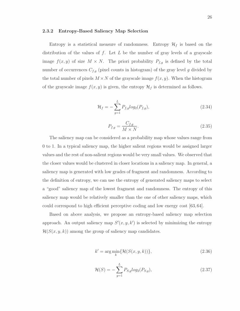
2.3.2 Entropy-Based Saliency Map Selection
Entropy is a statistical measure of randomness. Entropy Hf is based on the
distribution of the values of f . Let L be the number of gray levels of a grayscale
image f(x, y) of size M × N . The priori probability Pf,g is defined by the total
number of occurrences Cf,g (pixel counts in histogram) of the gray level g divided by
the total number of pixels M×N of the grayscale image f(x, y). When the histogram
of the grayscale image f(x, y) is given, the entropy Hf is determined as follows.
Hf = −L∑
g=1
Pf,glog2(Pf,g), (2.34)
Pf,g =Cf,g
M ×N. (2.35)
The saliency map can be considered as a probability map whose values range from
0 to 1. In a typical saliency map, the higher salient regions would be assigned larger
values and the rest of non-salient regions would be very small values. We observed that
the closer values would be clustered in closer locations in a saliency map. In general, a
saliency map is generated with low grades of fragment and randomness. According to
the definition of entropy, we can use the entropy of generated saliency maps to select
a “good” saliency map of the lowest fragment and randomness. The entropy of this
saliency map would be relatively smaller than the one of other saliency maps, which
could correspond to high efficient perceptive coding and low energy cost [63, 64].
Based on above analysis, we propose an entropy-based saliency map selection
approach. An output saliency map S ′(x, y, k′) is selected by minimizing the entropy
H(S(x, y, k)) among the group of saliency map candidates.
k′ = argmink
{H(S(x, y, k))}, (2.36)
H(S) = −L∑
g=1
PS,glog2(PS,g), (2.37)

27
PS,g =CS,g
M ×N, (2.38)
where H(S(x, y, k)) is the entropy of each saliency map candidate S(x, y, k).
2.3.3 Post-Processing
To achieve a better visual illustration, the final saliency map is generated after
some post-processing [10]. As introduced in [65], usually each element in the saliency
map is squared individually and then the saliency map is saliency map is convoluted
with a Gaussian burring kernel bopt(x, y) with an optimal sigma σopt determined by
experiments.
S ′′(x, y, k′) = bopt(x, y) � ‖S ′(x, y, k′)‖2, (2.39)
where bopt(x, y) is a Gaussian burring kernel with optimal sigma σopt, � denotes
the convolution operation and ‖ · ‖2 denotes the square of each element individually.
bopt(x, y) =1
2πσ2opt
exp
(−(x2 + y2)
2σ2opt
). (2.40)
We generate the kernel bopt(x, y) with the same size of the output saliency map by
sampling continuous Gaussian distributed values into discrete Gaussian distributed
values at the points of each pixel. The Gaussian values of this kernel are normalized
again by dividing each element by the sum of all elements in the kernel. In order to
further improve the output saliency map, other post-processing steps may be used,
e.g. border cut [38] and center-bias setting [26].
2.3.4 Visual Saliency Model Using Gamma Corrected Spectrum (GCS)
Gamma correction is a nonlinear operation used to modify the luminance or tris-
timulus values in an image display system [66]. It is defined by two reversible power
functions as follows.

28
Vout = (Vin)γ , (2.41)
Vin = (Vout)1
γ , (2.42)
where Vout and Vin are the input and output values. Under common illumination
conditions, the human visual systems follows an approximate power function, namely
the psychophysical power law, developed by Stanley S. Stevens [67]. Gamma correc-
tion is used to compensate for the human visual system, in order to maximize the use
of the bits or bandwidth according to how humans perceive light or color [66].
We propose a visual saliency model using Gamma Corrected Spectrum (GCS). A
set of gamma corrections with different gamma values γk are utilized to modify the
amplitude spectrum while keeping the phase spectrum unchanged. Saliency map can-
didates S(x, y, k) can be constructed by the inverse transform of the gamma corrected
amplitude spectrums AGCS(u, v, k) with the original phase spectrum P(u, v).
AGCS(u, v, k) = (A(u, v))γk , (2.43)
S(x, y, k) = T−1[(A(u, v))γk · exp(i · P(u, v))], (2.44)
S(x, y, k) = T−1[exp(L(u, v) · γk + i · P(u, v))], (2.45)
where k is an index k = {0, . . . , K} and γk = k16. K is determined by the largest
dimension of the size of the saliency map, K = �log4(max(H,W )) + 1, where W
and H are the width and height of the saliency map. For example, if the size of
the saliency map is 64 × 48, K = 4, k = {0, 1, 2, 3, 4}, and γk = {0, 116, 18, 14, 12}. An
output saliency map S ′(x, y, k′) is selected by minimizing the entropy H(S(x, y, k))
among the set of candidates using the same Equation (2.36) and (2.37). The final
GCS saliency map is generated by Equation (2.39).

29
2.3.5 Visual Saliency Model Using Gamma Corrected Log Spectrum (GCLS)
Following our Gamma Corrected Spectrum (GCS) model, we also develop a visual
saliency model using the Gamma Corrected Log Spectrum (GCLS). A set of gamma
corrections with different gamma values γk are used to modify the log amplitude
spectrum while keeping the phase spectrum unchanged. For convenience, we only
describe the main steps in the following equations.
LGCLS(u, v, k) = (L(u, v))γk , (2.46)
S(x, y, k) = T−1[exp((L(u, v))γk + i · P(u, v))], (2.47)
We use the same parameter settings as the GCS model and an output saliency
map S ′(x, y, k′) is generated by the same selection approach as Equation (2.36). The
final GCLS saliency map is obtained by Equation (2.39).
2.3.6 Visual Saliency Model Using Low-Pass Filtered Spectrum (LPFS)
The amplitude spectrum contains some information related to non-salient and
salient regions. ¿From our spectral analysis, the sharp peaks or spikes in the amplitude
spectrum are strongly related to repeated patterns (non-salient regions) while the
other entities correspond to distinct patterns (salient regions). In order to discard
non-salient regions and maintain the salient regions, a low-pass filter (LPF) can be
used to suppress sharp peaks or spikes to generate saliency map. We design a low-
pass filter LPF (u, v, k) in the frequency domain based on the k-th root of a two-
dimensional (2D) cosine function.
LPF (u, v, k) =
(1
4(1 + cos(u))(1 + cos(v))
) 1
k
, (2.48)
lpf(x, y, k) =
(1
16(δ(x− 1) + 2δ(x) + δ(x+ 1))(δ(y − 1) + 2δ(y) + δ(y + 1))
) 1
k
,(2.49)

30
where (u, v) ∈ [−π,+π] and 1kdenotes the k-th root of the 2D cosine function.
This low-pass filter with frequency response LPF (ej0, ej0) = 1, LPF (eju, e±jπ) = 0
and LPF (e±jπ, ejv) = 0 in the frequency domain. Note that when k = 1, this LPF
in the frequency domain corresponds to a 2D Finite Impulse Response (FIR) filter
lpf(x, y, 1) in the spatial domain.
LPF (u, v, 1) =1
4(1 + cos(u))(1 + cos(v)), (2.50)
lpf(x, y, 1) =1
16
⎡⎢⎢⎢⎣1 2 1
2 4 2
1 2 1
⎤⎥⎥⎥⎦ . (2.51)
This continuous low-pass filter in the frequency domain is sampled to generate a
discrete low-pass filter for each sampled frequency element. We remove the square
border elements within four lines on each side whose values equal or very close to
zero and then obtain a discrete low-pass filter LPF (u, v, k) with the same size of the
amplitude spectrum. The values of the sampled frequency elements are normalized
again by dividing each element by the sum of all elements in the LPF (u, v, k).
We propose a visual saliency model using Low-Pass Filtered Spectrum (LPFS). A
set of low-pass filters LPF (u, v, k) of various k-th roots of the 2D cosine function are
used to filter the amplitude spectrum while keeping the phase spectrum unchanged.
Saliency map candidates S(x, y, k) can be constructed by the inverse transform of
the Gaussian filtered amplitude spectrums ALPFS(u, v, k) with the original phase
spectrum P(u, v).
ALPFS(u, v, k) = A(u, v) � LPF (u, v, k), (2.52)
S(x, y, k) = T−1[A(u, v) � LPF (u, v, k) · exp(i · P(u, v))], (2.53)
where 1kdenotes the k-th root in the low-pass filter LPF (u, v, k) and k = 4n−1, n =
{1, . . . , N}. N is determined by the largest dimension of the size of the saliency
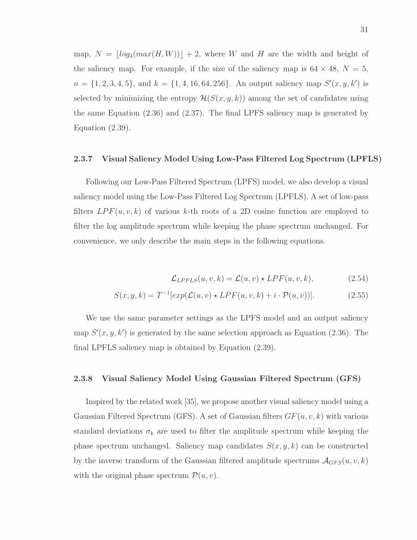
31
map, N = �log4(max(H,W )) + 2, where W and H are the width and height of
the saliency map. For example, if the size of the saliency map is 64 × 48, N = 5,
n = {1, 2, 3, 4, 5}, and k = {1, 4, 16, 64, 256}. An output saliency map S ′(x, y, k′) is
selected by minimizing the entropy H(S(x, y, k)) among the set of candidates using
the same Equation (2.36) and (2.37). The final LPFS saliency map is generated by
Equation (2.39).
2.3.7 Visual Saliency Model Using Low-Pass Filtered Log Spectrum (LPFLS)
Following our Low-Pass Filtered Spectrum (LPFS) model, we also develop a visual
saliency model using the Low-Pass Filtered Log Spectrum (LPFLS). A set of low-pass
filters LPF (u, v, k) of various k-th roots of a 2D cosine function are employed to
filter the log amplitude spectrum while keeping the phase spectrum unchanged. For
convenience, we only describe the main steps in the following equations.
LLPFLS(u, v, k) = L(u, v) � LPF (u, v, k), (2.54)
S(x, y, k) = T−1[exp(L(u, v) � LPF (u, v, k) + i · P(u, v))]. (2.55)
We use the same parameter settings as the LPFS model and an output saliency
map S ′(x, y, k′) is generated by the same selection approach as Equation (2.36). The
final LPFLS saliency map is obtained by Equation (2.39).
2.3.8 Visual Saliency Model Using Gaussian Filtered Spectrum (GFS)
Inspired by the related work [35], we propose another visual saliency model using a
Gaussian Filtered Spectrum (GFS). A set of Gaussian filters GF (u, v, k) with various
standard deviations σk are used to filter the amplitude spectrum while keeping the
phase spectrum unchanged. Saliency map candidates S(x, y, k) can be constructed
by the inverse transform of the Gaussian filtered amplitude spectrums AGFS(u, v, k)
with the original phase spectrum P(u, v).
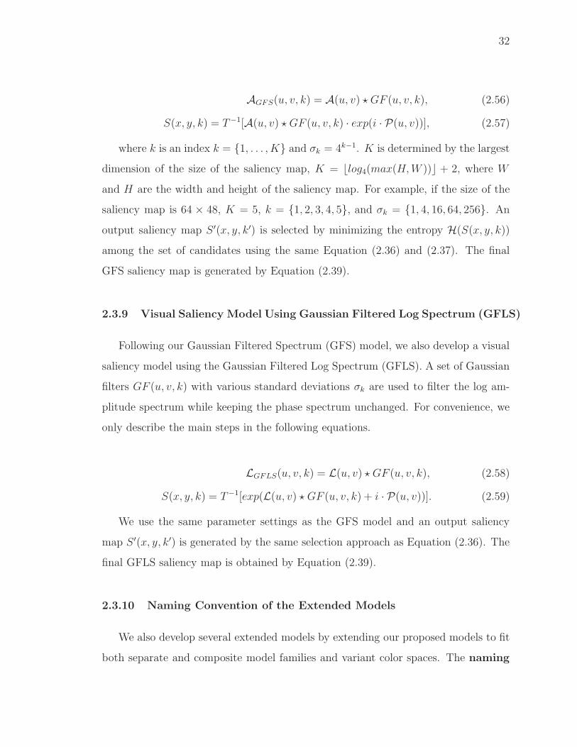
32
AGFS(u, v, k) = A(u, v) � GF (u, v, k), (2.56)
S(x, y, k) = T−1[A(u, v) � GF (u, v, k) · exp(i · P(u, v))], (2.57)
where k is an index k = {1, . . . , K} and σk = 4k−1. K is determined by the largest
dimension of the size of the saliency map, K = �log4(max(H,W )) + 2, where W
and H are the width and height of the saliency map. For example, if the size of the
saliency map is 64 × 48, K = 5, k = {1, 2, 3, 4, 5}, and σk = {1, 4, 16, 64, 256}. An
output saliency map S ′(x, y, k′) is selected by minimizing the entropy H(S(x, y, k))
among the set of candidates using the same Equation (2.36) and (2.37). The final
GFS saliency map is generated by Equation (2.39).
2.3.9 Visual Saliency Model Using Gaussian Filtered Log Spectrum (GFLS)
Following our Gaussian Filtered Spectrum (GFS) model, we also develop a visual
saliency model using the Gaussian Filtered Log Spectrum (GFLS). A set of Gaussian
filters GF (u, v, k) with various standard deviations σk are used to filter the log am-
plitude spectrum while keeping the phase spectrum unchanged. For convenience, we
only describe the main steps in the following equations.
LGFLS(u, v, k) = L(u, v) � GF (u, v, k), (2.58)
S(x, y, k) = T−1[exp(L(u, v) � GF (u, v, k) + i · P(u, v))]. (2.59)
We use the same parameter settings as the GFS model and an output saliency
map S ′(x, y, k′) is generated by the same selection approach as Equation (2.36). The
final GFLS saliency map is obtained by Equation (2.39).
2.3.10 Naming Convention of the Extended Models
We also develop several extended models by extending our proposed models to fit
both separate and composite model families and variant color spaces. The naming

33
convention of extended models is defined as “A-B-C”, where A represents a
proposed model’s abbreviation (i.e. GCS, GCLS, LPFS, LPFLS, GFS, and GFLS) or
an existing model’s abbreviation (i.e. IS and SSA); B represents a specific transform
used for an extended model (FT and DCT used for separate model family while
HFT used for composite model family); C represents a particular color space used
for an extended model, including Lab, IRGBY, and RGB color spaces.
2.3.11 Visual Saliency Model Evaluation
Popular evaluation measures for visual saliency model comparison are briefly re-
viewed. We discuss some challenges and open issues in model comparison and then
explained some ways to resolve them. Experimental results of comprehensive model
evaluations are shown next in Section 2.4.
The motivation for evaluating models with more than one measure is to ensure
that the main conclusions are independent of the choice of qualitative measures. A
ground-truth saliency map is denoted by G, which is based on the eye fixation array
of an image built by inserting 1s at fixation locations and 0s at the other locations.
The ground-truth saliency map G is usually computed by convoluting the eye fixation
array with a certain Gaussian kernel for smoothing. An estimated saliency map is
denoted by S, which is generated by a visual saliency model.
Normalized Scanpath Saliency (NSS)
Normalized scanpath saliency is the average of the response values at human eye
positions (xh, yh) in a model’s saliency map S [68]. Its values are normalized to have
zero mean and unit standard deviation.
NSS(G, S) =1
σS(S(xh, yh)− μS), (2.60)

34
where μS and σS are the mean and the standard deviation of the values in the
saliency map S. NSS is computed once for each saccade and subsequently the mean
and standard error are computed across the set of NSS scores. When NSS = 1, the
subjects’s eye positions fall in a region whose predicted saliency is one standard devi-
ation above average. NSS ≥ 1 indicates that the saliency map exhibits significantly
higher saliency values at human fixated locations compared to other locations. NSS
≤ 0 means that the model performs no better than picking a random position and
hence is at chance in predicting human gaze.
Kullback-Leibler (KL) Divergence
The KL divergence is usually used to measure distance between two probability
distributions. Using similar concept, it is used to measure the distance between
distributions of saliency values at human versus random eye positions [69, 70]. The
saliency magnitude at each sampled location is first normalized in the range [0, 1]. The
histogram of these magnitudes in l bins in the range [0, 1] across all eye movements
is calculated. Hk and Rk are the fraction of points in the bin k for salient and
random points respectively. The symmetric KL divergence (relative entropy) using
the difference between these histograms is defined as follows.
KL =1
2
l∑k=1
(Hklog2
(Hk
Rk
)+Rklog2
(Rk
Hk
)). (2.61)
Linear Correlation Coefficient (CC)
The linear correlation coefficient measures the strength of a linear relationship
between two saliency maps [71].
CC(G, S) =
∑x,y(G(x, y)− μG) · (S(x, y)− μS)√
σ2G · σ2
S
, (2.62)

35
where μG and μS are the means while σ2G and σ2
S are the variances of the G and S
saliency maps, respectively. When CC is close to +1 or 1 there is almost a perfectly
linear relationship between the two saliency maps.
Area Under The Curve (AUC)
AUC is the area under the Receiver Operating Characteristics (ROC) [72]. In the
context of saliency map evaluation, eye fixation points are considered as the positive
set and some points from the image are sampled to form the negative set [73]. The
saliency map S is then treated as a binary classifier to separate the positive samples
from the negative samples. By thresholding the saliency map at variant threshold
levels and plotting True Positive Rate (TPR) against False Positive Rate (FPR), an
ROC is obtained for each image.
TPR =TP
TP + FN, (2.63)
FPR =FP
FP + TN, (2.64)
where TP is the number of true positives, FP is the number of false positives, TN
is the number of true negatives, and FN is the number of false negatives. Figure 2.6
demonstrates the classification of true positive, false positive, true negative, and false
negative. The area underneath of each ROC is calculated for an image and the the
final AUC score is averaged over all images. Perfect prediction corresponds to a score
of 1 while a score of 0.5 indicates chance level.
Shuffled Area Under The Curve (sAUC)
As [10,38,73] pointed out, human eye fixations are often biased toward the center of
an image and this strong center-bias do significantly affect the performance evaluation
of visual saliency models using above evaluation measures. Based on [38,73], a shuffled
Area Under The Curve (sAUC) is proposed to resolve this issue. In order to remove
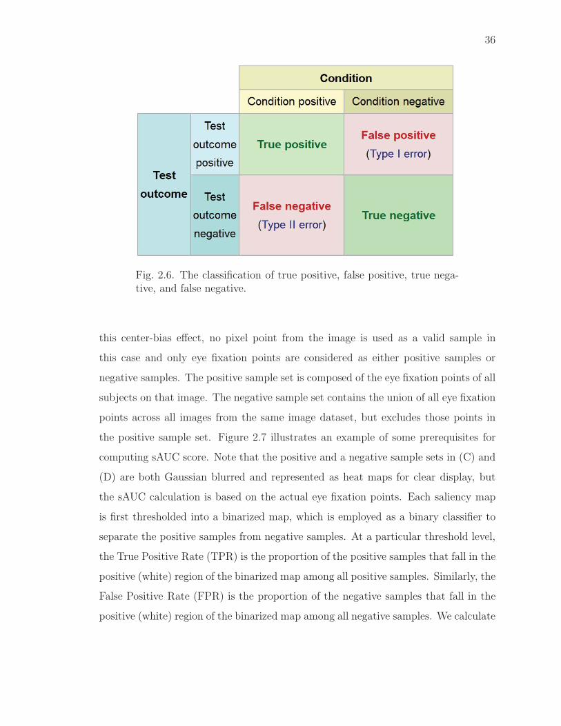
36
Fig. 2.6. The classification of true positive, false positive, true nega-tive, and false negative.
this center-bias effect, no pixel point from the image is used as a valid sample in
this case and only eye fixation points are considered as either positive samples or
negative samples. The positive sample set is composed of the eye fixation points of all
subjects on that image. The negative sample set contains the union of all eye fixation
points across all images from the same image dataset, but excludes those points in
the positive sample set. Figure 2.7 illustrates an example of some prerequisites for
computing sAUC score. Note that the positive and a negative sample sets in (C) and
(D) are both Gaussian blurred and represented as heat maps for clear display, but
the sAUC calculation is based on the actual eye fixation points. Each saliency map
is first thresholded into a binarized map, which is employed as a binary classifier to
separate the positive samples from negative samples. At a particular threshold level,
the True Positive Rate (TPR) is the proportion of the positive samples that fall in the
positive (white) region of the binarized map among all positive samples. Similarly, the
False Positive Rate (FPR) is the proportion of the negative samples that fall in the
positive (white) region of the binarized map among all negative samples. We calculate

37
a pair of TPR and FPR to obtain a point on the Receiver Operating Characteristics
(ROC) [72] (TPR versus FPR) based on a binarized map from a certain threshold.
TPR =TP
TP + FN, (2.65)
FPR =FP
FP + TN, (2.66)
where TP is the number of true positives, FP is the number of false positives,
TN is the number of true negatives, and FN is the number of false negatives.
Thresholding the saliency map at many threshold levels obtains a group of points
on the ROC and connecting these points yields a shuffled ROC. The area under this
curve is called the shuffled Area Under Curve (sAUC). The sAUC scores < 0.5
indicate a negative correlation while the sAUC scores > 0.5 indicate a positive
correlation. Perfect prediction leads to a sAUC score of 1.0 and chance level yields
0.5. Figure 2.8 demonstrates an example of the shuffled ROC used for computing the
sAUC score. The blue curve shows the shuffled ROC of the generated saliency map
for this image while the red reference line indicating the shuffled ROC of chance level.
The sAUC score of the black curve is 0.6329 and the one of the red reference line is
0.5.
All of above evaluation measures (except the sAUC) are significantly affected by
the center-bias and sAUC is more robust to center-bias and border effect [10]. The
sAUC score provides a good evaluation measure of the saliency map to accurately
predict where eye fixations occurred on an image. In order to fairly evaluate the
consistency between a saliency map and a set of fixations of an image dataset, we
employ shuffled Area Under Curve (sAUC) score as the evaluation measure in
our experiments.
2.3.12 Parameter Issues
Another issue regarding fair model comparison is how to adjust the parame-
ters of saliency models for different image datasets. It has been shown that blur-

38
Fig. 2.7. An example of some prerequisites for computing sAUC score.(A) The generated saliency map on a certain image, (B) The bina-rized saliency map thresholded at 0.5, (C) The positive sample setof eye fixation points only on this image (Gaussian blurred heat maprepresentation), (D) The negative sample set of eye fixation pointscontaining all fixation points across the entire image dataset but ex-cluding those points in the positive sample set (Gaussian blurred heatmap representation). Reproduced from [33]
ring/smoothing the resulting saliency maps has a significant influence on the sAUC
score of visual saliency models [33]. Some models provided the best settings of pa-
rameters for one image dataset, but sometime it’s not a good settings for other

39
Fig. 2.8. An example of the shuffled ROC used for computingthe sAUC score (true positive rate (TPR) versus false positive rate(FPR)). Reproduced from [33]
image datasets. We need to tune each model to achieve its best performance for
a certain image dataset by searching and selecting the optimal scale of Gaussian
blurring/smoothing. Ultimately, the model parameter issue will be better resolved
through an online challenge, where researchers can tune their own models to achieve
the best performance for different image datasets and share the resulting saliency
maps.

40
2.4 Experimental Results
Previous studies have shown that top-ranked visual saliency models are capable
of providing significantly accurate prediction of human eye fixation on natural images
in free viewing [7–10]. To evaluate the performance of our visual saliency models, we
did experiments to compare the proposed visual saliency models with some state-of-
the-art models. Our experiment is to use the proposed and existing visual saliency
models to predict human eye fixation on two standard image datasets. It should
be noted we did not do any actual eye fixation studies but used standard datasets.
We implemented all the extended models in MATLAB and set the saliency map’s
resolution to 64 × 48 pixels in all the experiments. We used the original MATLAB
implementation of models with the default settings and the recommended saliency
map’s resolution. The experiments were executed on a backend server with four
quad-core 3.2GHz CPU and 32GB RAM.
2.4.1 Predicting Eye Fixation
Eye Fixation Image Datasets
We adopted the shuffled AUC (sAUC) score [38, 73] as the evaluation measure
and developed an evaluation tool for benchmarking visual saliency models based on a
standard benchmark [33]. We did several experiments in predicting eye fixation using
two standard image datasets. (1) The Bruce and Tsotsos (BT) dataset [27] is the most
widely used dataset for comparing visual saliency models. It contains 120 color images
with resolution of 681x511 pixels from indoor and outdoor scenes and the eye fixation
data is based on 20 subjects. (2) The Li et al.’s (Li) dataset [35] is a new dataset
containing 235 color images with resolution of 640x480 pixels in six categories. 50
images with large salient regions, 80 with intermediate salient regions, 60 with small
salient regions, 15 with cluttered backgrounds, 15 with repeating distractors, and 15
with both large and small salient regions. Because blurring/smoothing the resulting

41
saliency maps is an important factor for fair comparison [33], we tune up each model
to achieve its best performance for above image datasets by searching and selecting
the optimal parameter of Gaussian blurring/smoothing. We blurred the saliency map
of each model by convoluting them with a series of Gaussian kernels with different
standard deviations σ (from 0.005 to 0.1 in steps of 0.005) in terms of the largest
dimension of an image. In our experiments, we kept all post-processing settings of
each model as original except the blurring/smoothing parameter.
Comparison of Extended Models
We made a systematic comparison of the six groups of 36 extended saliency models
that extends the proposed six visual saliency models by incorporating both separate
and composite model families and using variant color spaces. Note that naming
convention of extended models based on the six proposed models is provided in Sec-
tion 2.3.10. 18 FT-based extended models using the separate visual saliency model
family are compared with the baseline model SBVA(Itti) [25]. 18 HFT-based ex-
tended models using the composite visual saliency model family are also compared
with the baseline model SBVA(Itti) [25]. Based on the two standard image datasets,
Figure 2.9 and Figure 2.11 demonstrate the sAUC score of the FT-based extended
models while Figure 2.10 and Figure 2.12 illustrate the sAUC score of the HFT-based
extended models. Given the six groups of extended saliency models, the rank of
the extended models, the maximum sAUC score, and the optimal Gaussian standard
deviations σopt associated are shown in from Table 2.1 to Table 2.6. The results in-
dicate that the Lab and IRGBY color spaces work better with the FT-based models
in the separate model family and that the IRGBY color space works better with the
HFT-based models in the composite model family. Regarding the three color spaces,
Lab-based and IRGBY-based extended models are generally better than RGB-based
extended models in predicting human eye fixation. For the six groups of extended
saliency models, Table 2.7 shows the summary of the best extended models in the
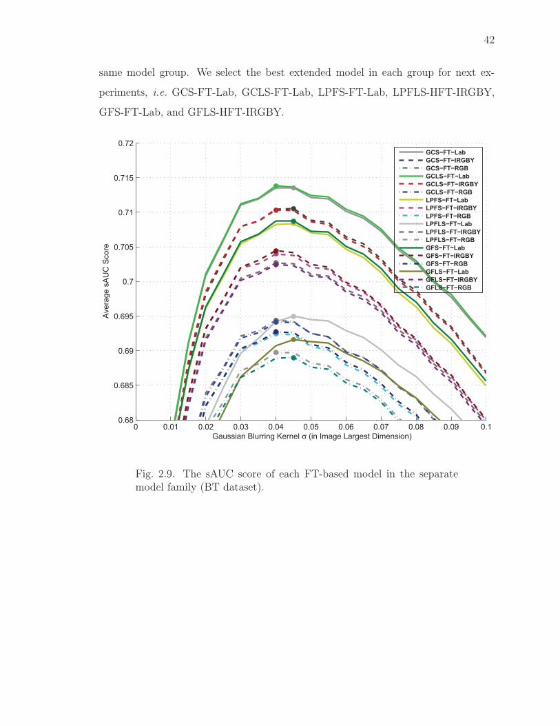
42
same model group. We select the best extended model in each group for next ex-
periments, i.e. GCS-FT-Lab, GCLS-FT-Lab, LPFS-FT-Lab, LPFLS-HFT-IRGBY,
GFS-FT-Lab, and GFLS-HFT-IRGBY.
0 0.01 0.02 0.03 0.04 0.05 0.06 0.07 0.08 0.09 0.10.68
0.685
0.69
0.695
0.7
0.705
0.71
0.715
0.72
Gaussian Blurring Kernel σ (in Image Largest Dimension)
Ave
rage
sA
UC
Sco
re
GCS−FT−LabGCS−FT−IRGBYGCS−FT−RGBGCLS−FT−LabGCLS−FT−IRGBYGCLS−FT−RGBLPFS−FT−LabLPFS−FT−IRGBYLPFS−FT−RGBLPFLS−FT−LabLPFLS−FT−IRGBYLPFLS−FT−RGBGFS−FT−LabGFS−FT−IRGBYGFS−FT−RGBGFLS−FT−LabGFLS−FT−IRGBYGFLS−FT−RGB
Fig. 2.9. The sAUC score of each FT-based model in the separatemodel family (BT dataset).

43
0 0.01 0.02 0.03 0.04 0.05 0.06 0.07 0.08 0.09 0.10.68
0.685
0.69
0.695
0.7
0.705
0.71
0.715
0.72
Gaussian Blurring Kernel σ (in Image Largest Dimension)
Ave
rage
sA
UC
Sco
re
GCS−HFT−LabGCS−HFT−IRGBYGCS−HFT−RGBGCLS−HFT−LabGCLS−HFT−IRGBYGCLS−HFT−RGBLPFS−HFT−LabLPFS−HFT−IRGBYLPFS−HFT−RGBLPFLS−HFT−LabLPFLS−HFT−IRGBYLPFLS−HFT−RGBGFS−HFT−LabGFS−HFT−IRGBYGFS−HFT−RGBGFLS−HFT−LabGFLS−HFT−IRGBYGFLS−HFT−RGB
Fig. 2.10. The sAUC score of each HFT-based model in the compositemodel family (BT dataset).

44
0 0.01 0.02 0.03 0.04 0.05 0.06 0.07 0.08 0.09 0.10.66
0.665
0.67
0.675
0.68
0.685
0.69
Gaussian Blurring Kernel σ (in Image Largest Dimension)
Ave
rage
sA
UC
Sco
re
GCS−FT−LabGCS−FT−IRGBYGCS−FT−RGBGCLS−FT−LabGCLS−FT−IRGBYGCLS−FT−RGBLPFS−FT−LabLPFS−FT−IRGBYLPFS−FT−RGBLPFLS−FT−LabLPFLS−FT−IRGBYLPFLS−FT−RGBGFS−FT−LabGFS−FT−IRGBYGFS−FT−RGBGFLS−FT−LabGFLS−FT−IRGBYGFLS−FT−RGB
Fig. 2.11. The sAUC score of each FT-based model in the separatemodel family (Li dataset).

45
0 0.01 0.02 0.03 0.04 0.05 0.06 0.07 0.08 0.09 0.10.66
0.665
0.67
0.675
0.68
0.685
0.69
Gaussian Blurring Kernel σ (in Image Largest Dimension)
Ave
rage
sA
UC
Sco
re
GCS−HFT−LabGCS−HFT−IRGBYGCS−HFT−RGBGCLS−HFT−LabGCLS−HFT−IRGBYGCLS−HFT−RGBLPFS−HFT−LabLPFS−HFT−IRGBYLPFS−HFT−RGBLPFLS−HFT−LabLPFLS−HFT−IRGBYLPFLS−HFT−RGBGFS−HFT−LabGFS−HFT−IRGBYGFS−HFT−RGBGFLS−HFT−LabGFLS−HFT−IRGBYGFLS−HFT−RGB
Fig. 2.12. The sAUC score of each HFT-based model in the compositemodel family (Li dataset).

46
Table 2.1The rank of extended GCS models, the maximum sAUC score, andthe associated Gaussian σopt (in image largest dimension).
Image GCS-FT GCS-HFT GCS-FT GCS-HFT GCS-FT GCS-HFT
Dataset -Lab -Lab -IRGBY -IRGBY -RGB -RGB
BT [27] Rank 1 3 2 4 6 5
Max sAUC 0.7135 0.7038 0.7105 0.7037 0.6944 0.6995
σopt 0.045 0.040 0.045 0.040 0.040 0.040
Li [35] Rank 1 5 3 2 6 4
Max sAUC 0.6805 0.6748 0.6786 0.6789 0.6739 0.6755
σopt 0.050 0.050 0.050 0.050 0.050 0.050
Table 2.2The rank of extended GCLS models, the maximum sAUC score, andthe associated Gaussian σopt (in image largest dimension).
Image GCLS-FT GCLS-HFT GCLS-FT GCLS-HFT GCLS-FT GCLS-HFT
Dataset -Lab -Lab -IRGBY -IRGBY -RGB -RGB
BT [27] Rank 1 4 2 3 6 5
Max sAUC 0.7138 0.7034 0.7103 0.7038 0.6941 0.6994
σopt 0.040 0.040 0.040 0.040 0.040 0.040
Li [35] Rank 1 5 3 2 6 4
Max sAUC 0.6803 0.6749 0.6779 0.6788 0.6736 0.6754
σopt 0.050 0.050 0.050 0.050 0.050 0.050

47
Table 2.3The rank of extended LPFS models, the maximum sAUC score, andthe associated Gaussian σopt (in image largest dimension).
Image LPFS-FT LPFS-HFT LPFS-FT LPFS-HFT LPFS-FT LPFS-HFT
Dataset -Lab -Lab -IRGBY -IRGBY -RGB -RGB
BT [27] Rank 1 3 2 4 6 5
Max sAUC 0.7084 0.7037 0.7040 0.7030 0.6924 0.6984
σopt 0.045 0.040 0.040 0.040 0.040 0.040
Li [35] Rank 2 4 3 1 6 5
Max sAUC 0.6767 0.6762 0.6775 0.6787 0.6718 0.6752
σopt 0.050 0.050 0.050 0.050 0.050 0.050
Table 2.4The rank of extended LPFLS models, the maximum sAUC score, andthe associated Gaussian σopt (in image largest dimension).
Image LPFLS-FT LPFLS-HFT LPFLS-FT LPFLS-HFT LPFLS-FT LPFLS-HFT
Dataset -Lab -Lab -IRGBY -IRGBY -RGB -RGB
BT [27] Rank 5 3 2 1 6 4
Max sAUC 0.6950 0.7010 0.7027 0.7031 0.6897 0.6985
σopt 0.045 0.045 0.040 0.040 0.040 0.040
Li [35] Rank 6 3 2 1 5 4
Max sAUC 0.6704 0.6766 0.6774 0.6787 0.6712 0.6751
σopt 0.045 0.050 0.050 0.050 0.050 0.050

48
Table 2.5The rank of extended GFS models, the maximum sAUC score, andthe associated Gaussian σopt (in image largest dimension).
Image GFS-FT GFS-HFT GFS-FT GFS-HFT GFS-FT GFS-HFT
Dataset -Lab -Lab -IRGBY -IRGBY -RGB -RGB
BT [27] Rank 1 3 2 4 6 5
Max sAUC 0.7087 0.7036 0.7044 0.7029 0.6927 0.6993
σopt 0.045 0.040 0.040 0.040 0.040 0.040
Li [35] Rank 2 4 2 1 6 5
Max sAUC 0.6780 0.6777 0.6780 0.6804 0.6727 0.6765
σopt 0.050 0.050 0.050 0.050 0.050 0.050
Table 2.6The rank of extended GFLS models, the maximum sAUC score, andthe associated Gaussian σopt (in image largest dimension).
Image GFLS-FT GFLS-HFT GFLS-FT GFLS-HFT GFLS-FT GFLS-HFT
Dataset -Lab -Lab -IRGBY -IRGBY -RGB -RGB
BT [27] Rank 5 3 2 1 6 4
Max sAUC 0.6916 0.7006 0.7024 0.7030 0.6890 0.6986
σopt 0.045 0.040 0.040 0.040 0.045 0.040
Li [35] Rank 6 3 2 1 5 4
Max sAUC 0.6695 0.6766 0.6772 0.6803 0.6719 0.6763
σopt 0.045 0.050 0.050 0.050 0.050 0.050

49
Table 2.7The summary of the best extended models: The rank in the samemodel group, the maximum sAUC score, and the associated Gaussianσopt (in image largest dimension).
Image GCS-FT GCLS-FT LPFS-FT LPFLS-HFT GFS-FT GFLS-HFT
Dataset -Lab -Lab -Lab -IRGBY -Lab -IRGBY
BT [27] Rank 1 1 1 1 1 1
Max sAUC 0.7135 0.7138 0.7084 0.7031 0.7087 0.7030
σopt 0.045 0.040 0.045 0.040 0.045 0.040
Li [35] Rank 1 1 2 1 2 1
Max sAUC 0.6805 0.6803 0.6767 0.6787 0.6780 0.6803
σopt 0.050 0.050 0.050 0.050 0.050 0.050

50
Comparison with Other Models
We did a comprehensive evaluation of the six best extended saliency models
(GCS-FT-Lab, GCLS-FT-Lab, LPFS-FT-Lab, LPFLS-HFT-IRGBY, GFS-FT-Lab,
and GFLS-HFT-IRGBY) by comparing with 10 saliency models from the literature
using two standard image datasets. The 10 models compared in this experiment are:
SBVA(Itti) [25], AIM [27], FTSD [29], PFDN [32], SR [65], PFT [30], PQFT [31],
QDCT [34], IS-DCT-Lab [33], SSA-HFT-IRGBY [35] The SBVA(Itti) and AIM are
spatial domain models while the FTSD, PFDN, SR, PFT, PQFT, IS-DCT-Lab, SSA-
HFT-IRGBY and the six best extended models are all frequency domain models.
Figure 2.13 and Figure 2.15 demonstrate the sAUC score of each model based on
the two standard image datasets. Figure 2.14 and Figure 2.16 illustrate the average
execution time per image of each model. Note that the time axis lower than 0.3
second uses a linear scale but it higher than 0.3 second is defined in a non-linear scale
based on the largest value of the average execution time per image. Figure 2.13 and
Figure 2.15 demonstrate the sAUC score of each model based on the two standard
image datasets. Figure 2.14 and Figure 2.16 illustrate the average execution time per
image of each model. Figure 2.17, Figure 2.18, and Figure 2.19 illustrate examples
of saliency maps from different visual saliency models for the same images in the BT
dataset. Figure 2.20, Figure 2.21, and Figure 2.22 illustrate examples of saliency maps
from different visual saliency models for the same images in the Li dataset. Note that
the table in the middle indicates the locations of the saliency maps corresponding to
which visual saliency models.
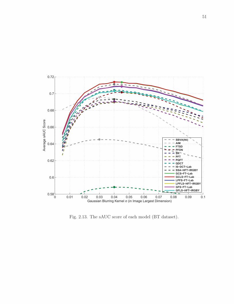
51
0 0.01 0.02 0.03 0.04 0.05 0.06 0.07 0.08 0.09 0.10.58
0.6
0.62
0.64
0.66
0.68
0.7
0.72
Gaussian Blurring Kernel σ (in Image Largest Dimension)
Ave
rage
sA
UC
Sco
re
SBVA(Itti)AIMFTSDPFDNSRPFTPQFTQDCTIS−DCT−LabSSA−HFT−IRGBYGCS−FT−LabGCLS−FT−LabLPFS−FT−LabLPFLS−HFT−IRGBYGFS−FT−LabGFLS−HFT−IRGBY
Fig. 2.13. The sAUC score of each model (BT dataset).

52
0.00
0.05
0.10
0.15
0.20
0.25
0.30
1.37
2.44
3.52
4.59
0.240
4.051
0.133 0.140
0.009 0.0080.019
0.0310.017
0.116
0.027 0.028
0.0570.067
0.0580.067
Visual Saliency Models
Ave
rage
Com
putin
g Ti
me
(Sec
ond)
======
SBVA(Itti)AIMFTSDPFDNSRPFTPQFTQDCTIS−DCT−LabSSA−HFT−IRGBYGCS−FT−LabGCLS−FT−LabLPFS−FT−LabLPFLS−HFT−IRGBYGFS−FT−LabGFLS−HFT−IRGBY
Fig. 2.14. The average execution time of each model (BT dataset).
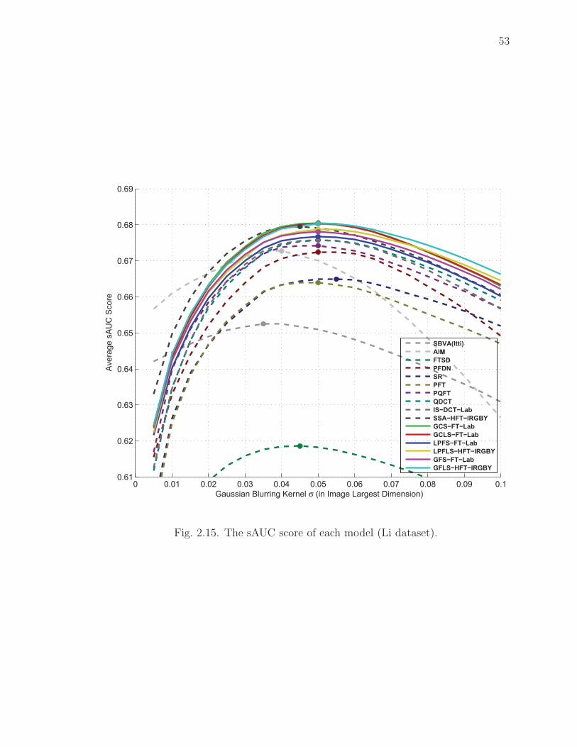
53
0 0.01 0.02 0.03 0.04 0.05 0.06 0.07 0.08 0.09 0.10.61
0.62
0.63
0.64
0.65
0.66
0.67
0.68
0.69
Gaussian Blurring Kernel σ (in Image Largest Dimension)
Ave
rage
sA
UC
Sco
re
SBVA(Itti)AIMFTSDPFDNSRPFTPQFTQDCTIS−DCT−LabSSA−HFT−IRGBYGCS−FT−LabGCLS−FT−LabLPFS−FT−LabLPFLS−HFT−IRGBYGFS−FT−LabGFLS−HFT−IRGBY
Fig. 2.15. The sAUC score of each model (Li dataset).

54
0.00
0.05
0.10
0.15
0.20
0.25
0.30
1.21
2.11
3.02
3.92
0.230
3.468
0.119
0.140
0.008 0.0070.018
0.0300.016
0.115
0.026 0.027
0.0550.066
0.0550.066
Visual Saliency Models
Ave
rage
Com
putin
g Ti
me
(Sec
ond)
======
SBVA(Itti)AIMFTSDPFDNSRPFTPQFTQDCTIS−DCT−LabSSA−HFT−IRGBYGCS−FT−LabGCLS−FT−LabLPFS−FT−LabLPFLS−HFT−IRGBYGFS−FT−LabGFLS−HFT−IRGBY
Fig. 2.16. The average execution time of each model (Li dataset).

55
Fig. 2.17. Examples of saliency maps from different models for twoimages (BT dataset).
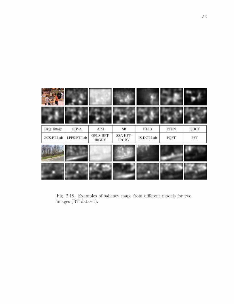
56
Fig. 2.18. Examples of saliency maps from different models for twoimages (BT dataset).
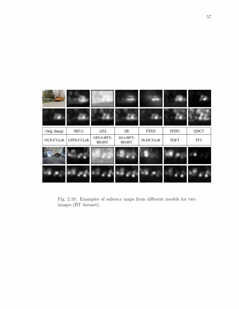
57
Fig. 2.19. Examples of saliency maps from different models for twoimages (BT dataset).
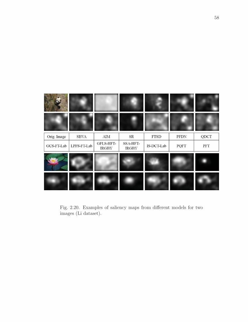
58
Fig. 2.20. Examples of saliency maps from different models for twoimages (Li dataset).

59
Fig. 2.21. Examples of saliency maps from different models for twoimages (Li dataset).
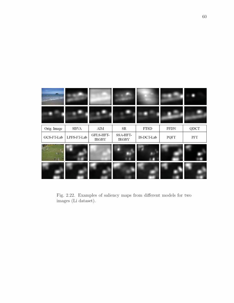
60
Fig. 2.22. Examples of saliency maps from different models for twoimages (Li dataset).
61
Table 2.8 shows the rank of each saliency model, the maximum sAUC score, and
the optimal Gaussian standard deviations σopt associated. The results show that
the six best extended models are generally better than most state-of-the-art models
because they are ranked in the top 8 out of all the 16 models for the BT dataset
and the top 7 out of all the 16 models for the Li dataset. Among the existing
models, IS-DCT-Lab [33], SSA-HFT-IRGBY [35], and QDCT [34] models performed
better than the rest while SBVA(Itti) [25], FTSD [29], SR [65], PFT [30] models
are ranked at the bottom. The proposed GCS-FT-Lab model has the highest sAUC
score for the Li dataset and is ranked the 2nd place among all models for the BT
dataset. The proposed GCLS-FT-Lab model has the highest sAUC score for the BT
dataset and is ranked the 2nd place among all models for the Li dataset. The QDCT
model has higher sAUC scores for the two datasets and it is ranked the 6th place
for the BT dataset and the 9th place for the Li dataset. The two spatial domain
models, SBVA(Itti) and AIM, have relatively low sAUC scores for the two datasets
and they are the two slowest models in terms of average computing time per image
in Figure 2.14 and Figure 2.16. For the BT dataset, SBVA(Itti) is about 8.9x slower
and AIM is about 150.0x than the proposed GCS-FT-Lab model. For the Li dataset,
SBVA(Itti) is about 8.8x slower and AIM is about 133.4x than the proposed GCS-
FT-Lab model. Moreover, the GCS-FT-Lab and GCLS-FT-Lab models are the two
most accurate ones in predicting eye fixation. Since the GCS-FT-Lab model has lower
complexity and is more efficient than GCLS-FT-Lab model, we select GCS-FT-Lab
model as the best one of all the 16 models.

62
Table 2.8The rank of each saliency model, the maximum sAUC score, and the associated Gaussian σopt (in imagelargest dimension).
Image SBVA AIM FTSD PFDN SR PFT PQFT QDCT IS-DCT SSA-HFT GCS-FT GCLS-FT LPFS-FT LPFLS-HFT GFS-FT GFLS-HFT
Dataset [25] [27] [29] [32] [65] [30] [31] [34] -Lab [33] -IRGBY [35] -Lab -Lab -Lab -IRGBY -Lab -IRGBY
BT [27] Rank 15 10 16 9 13 13 12 6 3 11 2 1 5 7 4 8
Max sAUC 0.6453 0.6956 0.5883 0.7015 0.6898 0.6898 0.6906 0.7041 0.7111 0.6932 0.7135 0.7138 0.7084 0.7031 0.7087 0.7030
σopt 0.030 0.030 0.040 0.045 0.040 0.040 0.040 0.040 0.040 0.040 0.045 0.040 0.045 0.040 0.045 0.040
Li [35] Rank 15 11 16 12 13 14 10 9 8 4 1 2 7 5 6 2
Max sAUC 0.6525 0.6727 0.6186 0.6724 0.6649 0.6639 0.6742 0.6757 0.6758 0.6795 0.6805 0.6803 0.6767 0.6787 0.6780 0.6803
σopt 0.035 0.040 0.045 0.050 0.055 0.050 0.050 0.050 0.050 0.045 0.050 0.050 0.050 0.050 0.050 0.050

63
Discussion
Our proposed GCS-FT-Lab and GCLS-FT-Lab models both achieve the top per-
formance for the two standard image datasets. Their performance is nearly consistent
over the two datasets but the performance of some visual saliency models vary over
different image datasets. The IS-DCT-Lab model [33] is among the top 3 models
for the BT dataset but results in average capability for the Li dataset. The SSA-
HFT-IRGBY model [35] is among the top 3 models for the Li dataset but performs
in the lower middle for the BT dataset. A reason could be that the two standard
image datasets have different distributions of eye fixation due to the characteristics
of the image datasets in terms of image/feature statistics, object/scene varieties, and
eye tracking biases. Figure 2.23 and Figure 2.24 illustrate the distribution and the
Gaussian blurred heat map representation of eye fixation of all the images in the two
datasets. The eye fixation of the BT dataset are less center-biased than the ones of
the Li dataset. We observed that the BT dataset images contain more sparse and
small salient objects while the Li dataset images include more dense and large salient
objects. This indicates that the IS-DCT-Lab model is good at detecting sparse and
small salient objects, the SSA-HFT-IRGBY model works better in capturing dense
and large salient objects, and the proposed GCS-FT-Lab model and GCLS-FT-Lab
models are good at both tasks.
Note that our GFLS-HFT-IRGBY model is similar to the SSA-HFT-IRGBY
model [35] using the same transform and color space. But it is different from the SSA-
HFT-IRGBY model in the way that the output saliency map is selected by minimizing
entropy directly. When the spectrum scale-space is constructed to select an optimal
scale for SSA-HFT-IRGBY model, an additional Gaussian kernel is used to filter each
saliency map candidate and then minimizing entropy is employed [35]. However, our
experimental results indicate that the additional Gaussian filtering provides a limited
benefit in predicting dense eye fixation but has a significant disadvantage in predicting
sparse eye fixation.

64
Fig. 2.23. The distribution of eye fixation of all the images in BTdataset (left) and Li dataset (right).
Fig. 2.24. The Gaussian blurred heat map representation of eye fix-ation of all the images in BT dataset (left) and Li dataset (right),where the Gaussian σ = 0.005 (in image largest dimension).

65
3. HAZMAT SIGN DETECTION AND RECOGNITION
USING VISUAL SALIENCY
Two typical hazmat signs used for a train tank car and a truck trailer are shown
in Figure 3.1. Hazmat signs have identifying visual information that can be distin-
guished from their surroundings by specific colors, shapes, symbols, and numbers.
However, there exist challenges for successful detection and recognition of hazmat
signs in complex scenes. Hazmat signs are usually divided into three separate parts
by placard holders with two horizontal strips. Various lighting and weather condi-
tions can deteriorate their color and shape over time. Additionally image distortions
may occur, such as blur and change in contrast.
(a) An example of haz-
mat sign used for a train
tank car.
(b) An example of a haz-
mat sign used for a truck
trailer.
Fig. 3.1. Examples of two hazmat signs divided into three separate parts.
In this chapter we describe a hazmat sign location detection and content recog-
nition system using visual saliency. In [14, 15] we reported some preliminary results
on this topic. We use saliency maps to denote regions likely containing hazmat signs
in complex scenes and use a convex quadrilateral shape detector to find hazmat sign
candidates in these regions. Based on our previous work [14, 15], we propose a new

66
approach to hazmat sign location detection using a new visual saliency model pro-
posed in Chapter 2 and a Fourier descriptor based contour matching method [74].
We use the best of our proposed frequency domain models to extract salient regions
that are likely to contain hazmat sign candidates and then use a Fourier descriptor
based contour matching method to locate the border of hazmat signs in these regions.
This visual saliency based approach is able to significantly increase the accuracy of
sign location detection, reduce the number of false positive objects, and speed up
the overall image analysis process. It uses contour-based shape representation and
correlation matching based on the magnitude and phase of the Fourier descriptor of
extracted contours. Closed contours are extracted from color channel images using
adaptive thresholding, image binarization, morphological operation and connected
component analysis. Experimental results show that our proposed hazmat sign lo-
cation detection method is capable of detecting and recognizing projective distorted,
blurred, and shaded hazmat signs in complex scenes.
3.1 Review of Existing Sign Detection and Recognition Methods
3.1.1 Sign Location Detection
Sign location detection approaches can be divided into three categories: color-
based methods [75], shape-based methods [76] and vision-based methods [24]. Color-
based methods take advantage of the fact that signs often have highly visible contrast-
ing colors. These specific colors are used for sign location detection. For example,
a color histogram backprojection method is used in [77] to detect interesting regions
possibly containing hazmat signs. In [78] sign location detection is performed using
a color-based segmentation method as a preprocessing step for shape detection. The
luminance homogeneity of blocks is used in [79] to identify homogenous regions as the
first step towards detection of information signs containing text. In [80] several color
components are used to segment traffic signs in various weather conditions. However,
color-based methods are not robust to lighting conditions and illumination changes.

67
Shape-based approaches first generate an edge map and then use shape charac-
teristics to find signs. For example, in [81] triangular, square and octagonal road
signs are detected by exploiting the properties of symmetry and edge orientations
exhibited by equiangular polygons. A shape classification method of a road-sign de-
tection system in [82] is based on linear and Gaussian-kernel support vector machines
(SVM). In [83] the authors present a system for detection and recognition of road
signs with red boundaries and black symbols inside. Pictograms are extracted from
the black regions and then matched against templates in a database. They propose
a fuzzy shape detector and a recognition approach that uses template matching to
recognize rotated and affine transformed road signs. In [84] the authors propose a
system for automatic detection and recognition of traffic signs based on maximally
stable extremal regions (MSERs) and a cascade of SVM classifiers trained using his-
togram of oriented gradient (HOG) features. The system works on images taken from
vehicles, operates under a range of weather conditions, runs at an average speed of
20 frames per second, and recognizes all classes of ideogram-based (nontext) traffic
symbols from an online road sign database. In most cases shape-based methods are
invariant to translation, rotation, and scaling, while in some situations to partial oc-
clusions. Because color-based or shape-based sign location detection methods have
both strengths and disadvantages, most color-based approaches take shape into ac-
count after using color features while some shape-based detectors also integrate some
color aspects.
Vision-based approaches approaches utilize selective visual attention models, which
imitate human early visual processing in order to overcome the above problems in
complex scenes. Many vision-based traffic sign location detection and analysis meth-
ods are using visual saliency models to generate saliency maps that denote areas
where signs are likely to be found [24]. For example, in [85] a saliency map of road
traffic signs is constructed by a weighted sum of color and edge feature maps. A
traffic sign recognition system in [86] uses a visual attention system to denote regions
with possible candidates. In our previous work [14, 15] we proposed several image

68
analysis methods using visual saliency for hazmat sign location detection and context
recognition. This extended work makes use of our proposed visual saliency models to
construct a saliency map as a part of hazmat sign location detection method.
3.1.2 Sign Recognition
Sign recognition methods can be classified into: geometric constraint methods,
boosted cascades of features, and statistical moments [24, 79, 87].
Methods based on geometric constraints include the use of Hough-like meth-
ods [88, 89], contour fitting [90, 91], or radial symmetry detectors [92, 93]. These
approaches apply constraints on the object to be detected, such as little or no affine
transformations, uniform contours, or uniform lightning conditions. Although these
conditions are usually met, they cannot be generalized. For example, [89] presents an
analysis of Hough-like methods and confirms that the detection of signs under real-
world conditions is still unstable. A novel Hough-like technique for detecting circular
and triangular shapes is also proposed, in order to overcome some of the limitations
exposed.
Methods based on the boosted cascades of features commonly use the Viola-
Jones framework [94–96]. These approaches often use object detectors with Haar-like
wavelets of different shapes, and produce better results when the feature set is large.
For example, in [95] a system for detection, tracking, and classification of U.S. speed
signs is presented. A classifier similar to the Viola-Jones detector is used to discard
objects other than speed signs in a dataset of more than 100,000 images. In [96]
the detection is based on a boosted detectors cascade, trained with a version of Ad-
aboost, which allows the use of large feature spaces. The system is robust to noise,
affine deformation, partial occlusions, and reduced illumination.
Methods based on statistical moments [97–99] use the central moments of the
projections of the object to be detected. They can be used to check the orientation of
the object, or to distinguish between different shapes such as circles, squares, triangles,

69
or octagons. These methods are not robust to projective distortions or non-uniform
lightning conditions. For example, in [99] a mobile-based sign interpretation system
uses detection of shapes with an approximate rotational symmetry, such as squares
or equilateral triangles. It is based on comparing the magnitude of the coefficients of
the Fourier series of the centralized moments of the Radon transform of the image
after segmentation. The experimental results show that the method is not robust to
projective distortions.
3.1.3 Shape Descriptors
Shape is an important low level object and image feature [76, 100–102]. Shape
can be described using “shape descriptor,” which can be generally classified into two
methods: contour-based methods and region-based methods [103]. Contour-based
methods only exploit the boundary information while region-based methods exploit
all the pixels within a region. Contour-based methods are widely used in many appli-
cations because of their computational efficiency but they may fail when objects have
low resolution. The Fourier descriptors (FD) is a classic and still popular method for
contour description [104, 105]. The key idea is to use the Fourier transform of the
periodic representation of the contour, which results in a shape descriptor in the fre-
quency domain. The low-frequency components of the descriptor contain information
about the general shape of the contour while the finer details are described in the high-
frequency components [74]. Although shape descriptors obtained from contour-based
methods are not generally robust to noise [106], the Fourier descriptor overcomes noise
sensitivity by usually using only the first few low frequency coefficients to describe
the shape [74, 103, 107]. The FD is also compact and easy to normalize. In addition,
it has been shown that the FD outperforms many other shape descriptors [106, 108].
Existing work on Fourier descriptor (FD) includes methods for generating de-
scriptors invariant to geometric transformations and matching methods for shape
similarity and matching. For example, a new Fourier descriptor for image retrieval

70
is proposed in [109] by exploiting the benefits of both the wavelet and Fourier trans-
forms. A complex wavelet transform is first used on the shape boundary and then the
Fourier transform of the wavelet coefficients at multiple scales is employed. Since FD
is used at multiple scales, the shape retrieval accuracy improves with respect to using
ordinary FD. FD feature vectors are analyzed for pedestrian shape representation
and recognition [110]. The results show that only ten descriptors of both low and
high frequency components of pedestrian and vehicle shapes are enough for accurate
shape recognition. The fast FD of some shapes are presented in [111] based on chain
codes and the Fourier transform for shape recognition. It is shown that the first ten
terms of Fourier coefficients are enough to approximate the shapes. In [74] a method
using the Fourier transform of local regions is developed to describe the contours in
these regions. A correlation-based contour matching method is also proposed in [74]
using both magnitude and phase information of Fourier descriptors for recognizing
road signs.
3.2 Review of Existing Hazmat Sign Detection and Recognition Systems
Although there exist several mobile-based applications that provide easy access
to the Emergency Response Guidebook (ERG) guidebook [1, 12], they only provide
manually browsing functionality. There are a few methods in the literature dealing
with sign detection and recognition, but we are only aware of two other published
papers with application to hazmat signs [77, 112].
3.2.1 Hazmat Sign Detection Based on SURF and HBP
In [77] the hazmat sign detection is done using color histogram back-projection
(HBP) and Speeded Up Robust Feature (SURF) [113] matching. The method was
implemented and tested on an autonomous mobile robot for the 2008 RoboCup World
Championship. Histogram back-projection is used to detect regions of interest in the
image and remove the background of the scene. A background image without a sign,
71
h(x, y), is used as a ground-truth to isolate the hazmat sign when it appears on the
scene and an image of it is captured, f(x, y). This is done by determining the euclidean
distance of the color coordinates of each pixel within h(x, y) and the corresponding
pixel within f(x, y). A threshold K is used to create a binary mask of the hazmat
sign by the use of an indicator function δ(x, y) = {(x, y) s.t. |f(x, y)− h(x, y)| > K}.Several color histograms are then estimated for the U and V channels on the YUV
color space, and summed up to create a single histogram Ho(U, V ) for every sign on
the image. A threshold θ(Ho, ε) is used for Ho(U, V ), resulting in a binary indicator
function πo(U, V ), which specifies which pixels form part of a sign. The value of ε is
manually set to 0.05. Finally, morphological filters are used to segment the masked
regions from the background and create one or more regions of interest to be used as
inputs to the matching process using SURF features.
SURF matching is used to find interest points and retrieve images from a database.
After the region of interest is determined from the image containing a hazmat signs,
multiple interest points are found using SURF. Interest points surrounding regions
that overlap the region of interest are discarded, since the do not provide enough infor-
mation about the sign. For the remaining interest points, their corresponding feature
vectors are matched against all features of all images in a database corresponding to
the colors found on the first step.
The experiments were done using a stereo camera system consisting of two cameras
with a resolution of 1024 × 768 pixels. The tests consisted of detecting five different
hazmat signs in 240 images. The images were taken at 1, 1.5 and 2 meters, with a
maximum distortion of 30◦. The results show a detection accuracy of 92% from 1
meter, 52% from 1.5 meters, and less than 20% from 2 meters. The running time
ranges from 1 to 1.6 second on a 2.7GHz Intel CPU.

72
3.2.2 Hazmat Sign Detection Based on HOG
In [112] hazmat sign detection using sliding windows and Histogram of Oriented
Gradients (HOG) [114] is described. The method was implemented and tested on a
wheeled USAR robot for the 2010 RoboCup World Championship.
The authors use the sliding window approach to exhaustively scan every pixel
over a range of positions and scales, with steps of 8 pixels and relative scale factors
of 1.05. For each position and scale a discriminative Support Vector Machine (SVM)
classifier is used to make binary decisions about the presence or absence of an object.
In order to describe the contents of the image at each particular location a HOG
descriptor is used along with color histograms in the Lab color space to distinguish
between multiple hazmat signs. For each hazmat sign hypothesis of the HOG based
detector, the color histogram is used to do the final classification by applying a k-
nearest neighbor approach in combination with χ2-distance.
The experimental results show a recognition rate of 37.5% using histograms based
on entire sliding windows and a recognition rate of 58.3% using sub-region based
histograms. Region-based histograms provide better representation of the image since
they are capable of capturing the spatial distribution of colors within the detection
window.
3.2.3 Comparison to MERGE
We proposed a hazmat sign location detection and content recognition system,
known as MERGE (Mobile Emergency Response GuidE) [13]. Although all methods
above are deployed on mobile environments, MERGE is intended for real-time use
by first responders, while [77] and [112] were intended for use in a very specific
context. The sign detection method proposed in [77] uses a ground-truth image
of the background to aid in detection when the hazmat sign appears. This is not a
feasible assumption in MERGE, since the first responders are expected to take images
of hazmat signs in a large variety of scenarios. In [112] a dataset of 1480 daylight
73
images is used for both people and hazmat sign recognition. However, the authors do
not specify how many images contain hazmat signs, or at what distances the signs
are located. They do not provide information about the resolution of the images or
the cameras used for acquisition. In MERGE no assumptions on the background
are made in order to detect the sign. Instead, color information is used to detect
candidate regions using a saliency map model.
Once the hazmat sign is detected [77] uses image matching based on SURF fea-
tures, and [112] uses HOG and color histogram descriptors, both being very time
consuming task. This step is not done in MERGE. Currently, the color of the hazmat
sign is considered to be uniform, and the detection is made at different color channels.
The recognition of non-uniformly-colored placards is presented as part of the future
work.
The goal of MERGE is to be able to detect hazmat signs at long distances. Our
experimental results show successfully detecting hazmat signs in some cases at more
than 100 feet. However, the experiments in [77] can only be considered successful at
1.5 meters, and the accuracy reported by [112] is very low. Finally, the execution
time of the overall process of our hazmat sign image analysis system MERGE is
several seconds, comparable with the hazmat sign image analysis system in [77]. No
execution time is reported in [112].
74
3.3 Proposed Hazmat Sign Detection and Recognition System
3.3.1 MERGE System Overview1
Figure 3.2 shows the overview of our proposed hazmat sign location detection
and content recognition system, known as MERGE (Mobile Emergency Response
GuidE) [13]. It consists of an application running on an Android/iOS mobile device2
and a backend server where many image analysis operations are done [14,15]. There
are two basic operational modes of our MERGE system: analysis of hazmat sign
images and searching internal database. The first mode includes capturing or selecting
an hazmat sign image from the mobile device and performing image analysis on the
backend server. Hazmat sign detection and recognition are done on the backend
server and the results are sent back to the mobile device [14, 15]. The second mode
includes searching the internal database to obtain guide information about a specific
hazmat sign. We designed an internal database based on the contents of the 2012
ERG guidebook. As shown in Figure 3.3, hazmat signs can be manually searched by
UN identifier numbers, template images, symbols, and classes.
Figure 3.4 shows the operational workflow and user interface at each step. The
image analysis results are used for matching related guide pages and querying internal
database to retrieve guide information. We display guide information about poten-
tial hazards, public safety and emergency response. All the information is from the
internal database on the mobile application. A suggested evacuation region is also
displayed on a map based on the chemical found, the size of the chemical spill, the
time of the day, and a weather-aware chemical spreading webservice.
1The work in this section was developed by the author jointly with my colleagues Albert Parra
and Joonsoo Kim.2The Android application was developed by my colleague Albert Parra and the iOS application
was developed by my colleague Joonsoo Kim.
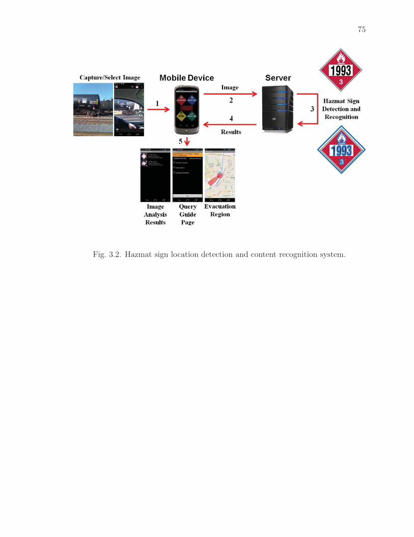
75
Fig. 3.2. Hazmat sign location detection and content recognition system.
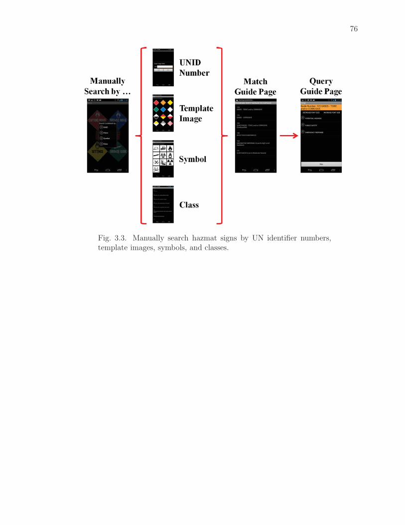
76
Fig. 3.3. Manually search hazmat signs by UN identifier numbers,template images, symbols, and classes.
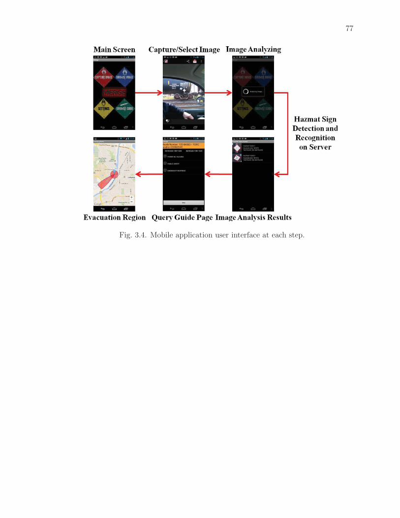
77
Fig. 3.4. Mobile application user interface at each step.

78
3.4 Hazmat Sign Detection and Recognition Method 1
We use visual saliency based methods and generate saliency maps using color
spaces. Spatial domain visual saliency models usually have high computational cost
and variant parameters for multiple feature maps, which make them impractical to
meet our needs. Frequency domain visual saliency models with fast computation
with high prediction accuracy could be suitable for our application. Our proposed
hazmat sign detection and recognition method is based on visual saliency. We use
two existing visual saliency models to generate saliency maps denoting salient regions
likely containing hazmat signs in complex scenes and develop a convex quadrilateral
shape detection method to extract the border of hazmat signs in these regions. The
block diagram in Figure 3.5 shows the building blocks of the proposed hazmat sign
detection and recognition method 1.
Fig. 3.5. Proposed hazmat sign detection and recognition method 1.

79
3.4.1 Saliency Map Generation
We use two existing visual saliency models to generate saliency maps from images
represented in both Lab and RGB color spaces, because we observed that color signs
have strong visual responses in Lab color space while white signs have strong visual
responses in RGB color space from our experiments. In each color space, two saliency
maps are generated separately using two visual saliency models, i.e. IS model [33]
and SSA model [35] respectively. The saliency maps assign higher saliency value
(ranging from lowest 0 to highest 1) to more visually attractive regions that are
likely containing hazmat signs in complex scenes. Note that the original SSA method
uses the IRGBY color space [35]. We modified this method to use Lab and RGB
color components with different weights ([12, 14, 14] for Lab and [1
3, 13, 13] for RGB). The
proposed hazmat sign detection method using the four saliency maps (two from Lab
and two from RGB), denoted as the combined method IS+SSA(Lab+RGB), has good
performance in the experiments. (see Section 3.6)
3.4.2 Salient Region Extraction
We threshold each saliency map to create a binary mask to extract the salient
regions from the original image. The threshold T1 is determined as k times the
average saliency value of a given saliency map.
T1 =k
W ×H
W∑x=1
H∑y=1
S(x, y), (3.1)
where W and H are the width and height of the saliency map, S(x, y) is the
saliency value at position (x, y) and k is empirically determined for the combined
detection method IS+SSA(Lab+RGB), i.e. k = 4.5 for IS models and k = 3.5 for
SSA models, which provides a good trade-off between hazmat sign coverage and com-
putational cost of extracted salient regions in the experiments. (see Section 3.6) The
80
following processing can take advantages of local distinctive features in the extracted
salient regions instead of the entire input image.
3.4.3 Convex Quadrilateral Shape Detection3
For each salient region found, we detect hazmat sign candidates in specific color
channels. We used black and white information from grayscale image, and red, green
and blue channels from RGB color space. Note that the possible colors for hazmat
signs also include yellow and orange, but these can be obtained by transforming
the image from RGB to a hue-based color space and then segment the hue channel.
The grayscale image and the color channels are thresholded to account for highly
chromatic areas using an empirically determined threshold T2 (85 for black, 170 for
white, and 127 for color). Each binarized region is morphologically opened to remove
small objects and morphologically dilated to merge areas that may belong to the
same object. We then retrieve contours from the resulting binary image using the
border following technique proposed in [115]. For each contour, we use the Hough
Transform [116] to find straight lines that approximate the contour as a polygon. The
intersections of these lines are the corners of the polygon which can be used to discard
non-quadrilateral shapes. If the contour is approximated by four vertices, we find its
convex hull [117]. If the convex hull still has four vertices, we check the angles formed
by the intersection of its points. If each of these angles is in the range 90◦± 1.5◦, and
the ratio of the sides formed by the convex hull is in the range 1 ± 0.5, we assume
that the convex quadrilateral is a hazmat sign candidate.
3.4.4 Duplicate Sign Removal
To remove duplicate sign candidates from different color channel images, we first
check all candidates passed the contour matching and estimate their minimal bound-
ing boxes. Any disqualified candidate with the aspect ratio of its bounding box
3The work in this section was developed by the author jointly with my colleague Albert Parra.

81
greater than 1.3 will be discarded. We then remove the duplicate sign candidates
that correspond to the same sign. This can be done by first dividing all candidates
that are overlapped more than 50% into multiple groups and then finding the optimal
diamond-shaped box for each group, whose four nodes are closest to the centroid of
its group. Each optimal diamond-shaped box is considered to be the location of a
detected hazmat sign.
3.4.5 Color Recognition4
Because signs are detected in specific color channels, the color is recognized directly
from the color channel where the sign was identified (black or white for grayscale and
red, green or blue for RGB). The recognized color is used for queuing the mobile
database for sign category identification and providing the general guide information
based on the 2012 ERG guidebook. Figure 3.6(a) illustrates a successful detection
of two signs using the previous Method 1, one of which is affected by projective and
rotational distortion. Figure 3.6(b) illustrates a true positive and a false positive from
the previous Method 1.
(a) Two true positives. (b) One true positive and one false positive.
Fig. 3.6. Examples of image analysis.
4The work in this section was developed by the author jointly with my colleague Albert Parra.

82
3.5 Hazmat Sign Detection and Recognition Method 2
We use our proposed frequency domain models in Chapter 2 to extract salient
regions that are likely to contain hazmat sign candidates and develop a Fourier de-
scriptor based contour matching method to extract the border of hazmat signs in these
regions. Based on our previous work [14], we propose a new approach to hazmat sign
location detection using a Fourier descriptor based contour matching method [74].
It uses contour-based shape representation and correlation matching based on the
magnitude and phase of the Fourier descriptor of extracted contours. The existing
method used to detect road signs in [74] cannot be directly used for hazmat sign
location detection. Hazmat signs mounted on vehicles are usually enclosed in a plac-
ard holders with two horizontal strips that divide a hazmat sign into three separate
parts as shown in Figure 3.1. In our case we need to use morphological operations to
merge separate parts that belong to a whole hazmat sign and then employ connected
component analysis to determine the boundary of the whole hazmat sign. Closed
contours are extracted from color channel images using adaptive thresholding, image
binarization, morphological operation and connected component analysis.
Fourier Descriptor (FD) is used to describe the shape of the extracted contours
through the Fourier transform [104, 105]. It has been proven to be a state-of-the-art
contour-based sign detection methods in terms of accuracy and tolerance of rotated,
scaled, and noisy signs [74, 105, 110]. In order to determine if an extracted contour
correspond to a hazmat sign, we need to compare its FD against the FD of the
contour of a shape template or a predefined shape contour. In our case, the shape
template of hazmat signs is represented by a diamond shaped binary image as shown
in Figure 3.7.
Contour matching can be done in the spatial or frequency domain. We use match-
ing in the frequency domain for two reasons. First, matching in the frequency domain
is scale independent, as opposed to spatial domain matching. Second, matching in
the spatial domain involves scanning an image multiple times modifying the scale

83
Fig. 3.7. A diamond shaped binary image represents the shape tem-plate of a hazmat sign.
and rotation of the shape template. Frequency domain matching methods have been
shown to be more computationally efficient when working with images of high res-
olution [118, 119]. FD-based matching is usually done by using only the magnitude
and ignoring the phase information. By discarding the phase information, rotation
and starting point invariance can be achieved [120]. However, because variant shapes
can have similar magnitude but different phase information, this makes FD-based
magnitude-only matching less accurate [74]. A correlation-based contour matching
method is proposed in [74] using both magnitude and phase information of Fourier
descriptors for recognizing road signs. It is shown that the normalized FDs are invari-
ant to scaling and the correlation-based contour matching using both magnitude and
phase information is invariant to rotation and starting point. We use this frequency
domain contour matching method [74] to detect the location of hazmat signs based
on a diamond shaped template. The block diagram in Figure 3.8 shows the building
blocks of the proposed hazmat sign detection and recognition method 2.
3.5.1 Saliency Map Generation
We use our proposed frequency domain models to generate saliency maps from
input images represented in both Lab and RGB color spaces, because we observed
that color signs have strong visual responses in Lab color space while white signs
have strong visual responses in RGB color space from our experiments. In each color
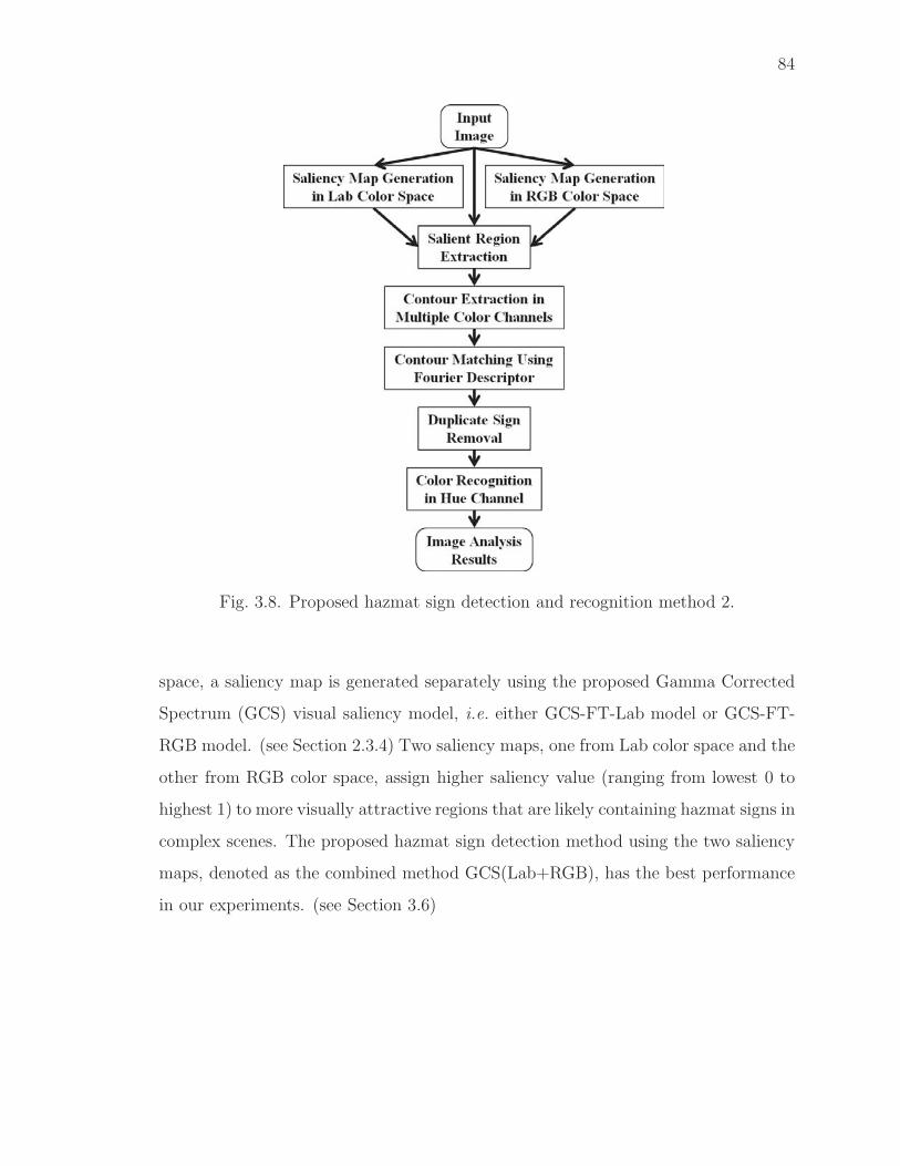
84
Fig. 3.8. Proposed hazmat sign detection and recognition method 2.
space, a saliency map is generated separately using the proposed Gamma Corrected
Spectrum (GCS) visual saliency model, i.e. either GCS-FT-Lab model or GCS-FT-
RGB model. (see Section 2.3.4) Two saliency maps, one from Lab color space and the
other from RGB color space, assign higher saliency value (ranging from lowest 0 to
highest 1) to more visually attractive regions that are likely containing hazmat signs in
complex scenes. The proposed hazmat sign detection method using the two saliency
maps, denoted as the combined method GCS(Lab+RGB), has the best performance
in our experiments. (see Section 3.6)

85
3.5.2 Salient Region Extraction
We threshold each saliency map to create a binary mask to extract the salient
regions from the original image. The threshold T1 is determined as k times the
average saliency value of a given saliency map.
T1 =k
W ×H
W∑x=1
H∑y=1
S(x, y), (3.2)
where W and H are the width and height of the saliency map, S(x, y) is the
saliency value at position (x, y) and k is empirically determined for the combined
detection method GCS(Lab+RGB), i.e. k = 2.0 for GCS-FT-Lab model and k =
2.0 for GCS-FT-RGB model, which provides a good trade-off between hazmat sign
coverage and computational cost in extracted salient regions in our experiments. (see
Section 3.6) The following processing can take advantages of local distinctive features
in the extracted salient regions instead of the entire input image.
3.5.3 Contour Extraction
The hazmat signs in our dataset contain either one or two of the following colors:
white, red, green, blue, and yellow. In order to obtain strong visual responses of
certain colors of hazmat signs, we transform an extracted salient region of the input
image into several channel images in different color spaces. The white signs can
be detected in the grayscale channel image. The red, green and blue signs can be
detected in R, G, B channel images from the RGB color space. The yellow signs can
be detected in the Y channel image from the CMYK color space. We process each
channel image of the extracted salient region separately in the following.
In order to binarize each channel image of the salient region ASRk , we propose
a new adaptive thresholding method that is a modification of Otsu’s thresholding
method [121]. Since images containing hazmat signs are likely acquired with various
lighting conditions, directly using Otsu’s thresholding method on the channel image

86
does not produce accurate results when images contain variable illumination [122].
For each channel image, Ii, i ∈ [1, 5], we first use a histogram of 256 bins for the
[0,255] grayscale values to characterize pixel distribution and then obtain the median
of the pixel counts of all bins NMEDi . Second, we find the starting location of two
significant peaks TLi and TH
i at the low and high ends of the histogram by checking
the change of pixel counts between two adjoining bins. The two index thresholds TLi
and THi are selected to clip the histogram.
NMEDi = median
(N (Bji )), (3.3)
TLi = argminj
(|N (Bji )−N (Bj
i − 1)| > FB ·NMEDi
), j ∈ [3, 128], (3.4)
THi = argmaxj
(|N (Bji )−N (Bj
i + 1)| > FB ·NMEDi
), j ∈ [129, 254],(3.5)
where N (Bji ) is the pixel count of the j-th bin in the histogram of the i-th channel
image, FB = 0.05 is a factor to determine index thresholds TLi and TH
i with respect
to NMEDi (empirically obtained by searching good values in our experiments), TL
i is
the starting location of the low-end significant peak (the index threshold of a low-
end bin), and THi is the starting location of the high-end significant peak (the index
threshold of a high-end bin). For each color channel image, we modify its histogram
by clipping the pixel counts N (Bji ) of the low-end and high-end bins into 0s based
on the two index thresholds TLi and TH
i .
N ′(Bji ) =
⎧⎨⎩ 0 Bj
i ≤ TLi or Bj
i ≥ THi
N (Bji ) otherwise
(3.6)
The modified histogram with new pixel counts N ′(Bji ) for all 256 bins is used with
the original Otsu’s method [121] to generate an adaptive threshold TBWi . Finally,
each original channel image Ii is then binarized using TBWi . Figure 3.9 illustrates
an example of image binarization using the proposed adaptive thresholding method
comparing with using Ostu’s method for a red channel image of an extracted salient
region. Note that our proposed adaptive thresholding method is capable of adapting
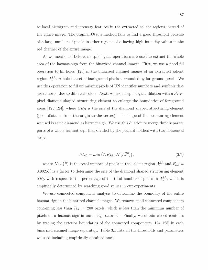
87
to local histogram and intensity features in the extracted salient regions instead of
the entire image. The original Otsu’s method fails to find a good threshold because
of a large number of pixels in other regions also having high intensity values in the
red channel of the entire image.
As we mentioned before, morphological operations are used to extract the whole
area of the hazmat sign from the binarized channel images. First, we use a flood-fill
operation to fill holes [123] in the binarized channel images of an extracted salient
region ASRk . A hole is a set of background pixels surrounded by foreground pixels. We
use this operation to fill up missing pixels of UN identifier numbers and symbols that
are removed due to different colors. Next, we use morphological dilation with a SED-
pixel diamond shaped structuring element to enlarge the boundaries of foreground
areas [123, 124], where SED is the size of the diamond shaped structuring element
(pixel distance from the origin to the vertex). The shape of the structuring element
we used is same diamond as hazmat sign. We use this dilation to merge three separate
parts of a whole hazmat sign that divided by the placard holders with two horizontal
strips.
SED = min(7, FSE · N (ASR
k )), (3.7)
where N (ASRk ) is the total number of pixels in the salient region ASR
k and FSE =
0.0025% is a factor to determine the size of the diamond shaped structuring element
SED with respect to the percentage of the total number of pixels in ASRk , which is
empirically determined by searching good values in our experiments.
We use connected component analysis to determine the boundary of the entire
hazmat sign in the binarized channel images. We remove small connected components
containing less than TCC = 200 pixels, which is less than the minimum number of
pixels on a hazmat sign in our image datasets. Finally, we obtain closed contours
by tracing the exterior boundaries of the connected components [124, 125] in each
binarized channel image separately. Table 3.1 lists all the thresholds and parameters
we used including empirically obtained ones.

88
Table 3.1Thresholds and parameters used in our proposed method. Automat-ically determined ones are denoted by *.
Symbol Description Value
NMEDi Median of the pixel counts of all bins *
TLi Low index threshold to clip the histogram *
THi High index threshold to clip the histogram *
TBWi Adaptive threshold to binarize channel images *
SED Size of the diamond shaped structuring element *
FB Factor to determine index thresholds TLi and TH
i 0.05
FSE Factor to determine the size of the structuring element SED 0.0025%
TCC Threshold to remove small connected components 200
Te Threshold for correlation-based matching cost e 1.751

89
(a) Original image (b) Extracted saliency regions
(c) Histogram of the saliency region in red channel
(d) Otsu’s method (e) Proposed method
Fig. 3.9. Example of image binarization using the proposed adaptivethresholding method comparing with using Ostu’s method.
90
3.5.4 Fourier Descriptor Generation
The Fourier Descriptor (FD) describes the shape of an object using a set of the
Fourier transform coefficients of the object’s contour [104, 105]. Given the extracted
contour c(k) has N pixels, numbered from 0 to N − 1, a set of pixel coordinates
describing the contour c(k) can be defined as follows.
c(k) = (x(k), y(k)) = x(k) + iy(k), (3.8)
where k = 0, 1, 2, . . . , N − 1. The Fourier transform of the contour points c(k)
generates a set of complex numbers C(v) which are the Fourier descriptors of the
contour.
C(v) = F(c(k)) =1
N
N−1∑k=0
c(k)exp
(−i2πvk
N
), (3.9)
where v = 0, 1, 2, . . . , N − 1. In order to describe the shape of a closed contour
generally, the Fourier descriptor have to be modified to make it invariant to translation
and scaling [74,109–111]. To achieve translation invariance, the DC Fourier coefficient
C(0) is set to zero C(0) = 0. All points on the contour are then shifted from its original
coordinate to (0, 0). The closed contour represented by the remaining Alternating
Current (AC) Fourier coefficients is invariant against translation, but it’s still affected
by scaling due to the magnitude of each AC coefficient. To achieve scaling invariance,
the remaining AC Fourier coefficients C(v) are normalized by√∑N−1
v=1 |C(v)|2. The
modified Fourier descriptor C ′(v) of the extracted contour c(k) are obtained as follows.
C ′(v) =
⎧⎨⎩
0, if v = 0,
C(v)√∑N−1
v=1|C(v)|2
, if v �= 0,(3.10)
where C(v) is the original Fourier coefficients. The low frequency components of
Fourier descriptors C ′(v) contain information about the general shape of the contour
while the high frequency components contain finer details. Therefore, the first P
91
modified AC Fourier descriptors can be used to create an approximate reconstruction
b(k) of the original contour points c(k) for contour matching.
c(k) =1
P
P∑v=0
C ′(v)exp(i2πvk
N
), (3.11)
where k = 0, 1, 2, . . . , N − 1.
3.5.5 Correlation-Based Contour Matching5
We use the correlation-based contour matching method [74] to locate the border of
hazmat signs based on a diamond shaped template. To achieve the rotation and start-
ing point invariance, the correlation-based contour matching using both magnitude
and phase information is required for hazmat sign location detection. The mod-
ified Fourier descriptors of extracted contours and the template contour can been
obtained in previous steps and their magnitude and phase information is used to
compute cross-correlation by employing complex conjugate multiplication XY . This
correlation-based contour matching method is able to achieve translation, scaling, ro-
tation and starting point variances. The cross-correlation rTE(l) between an extracted
contour cE and the template contour cT is defined as follows.
rTE(l) =
∫ K
0
cT (k)cE(l + k)dk
=N−1∑v=0
C ′T (v)C′E(v)exp
(−i2πvl
K
)(3.12)
= F−1{C ′TC ′E}(v). (3.13)
By using the first P modified Alternating Current (AC) Fourier descriptors with
both magnitude and phase information, this simplified contour matching method is
5The work in this section was developed by the author jointly with my colleague Kharittha
Thongkor.

92
able to approximately achieve translation, scaling, rotation and starting point vari-
ances. We say “approximately” because we are only using the first few modified
Fourier descriptors to describe the shape of the closed contour. In order to determine
the appropriate number P of modified AC Fourier descriptors needed for contour
matching, we examined the shape variations from a group of reconstructed contours of
the template diamond-shaped contour by varying the number of modified AC Fourier
descriptors we used. Figure 3.10 illustrates the shape variations of using the first 4,
8, 16, 32, 50 and 100 modified AC Fourier descriptors to reconstruct the template
contour of diamond shape. It is shown that using the first 8 modified AC Fourier
descriptors is a good approximation of the contour of the diamond shaped template.
Using more Fourier descriptors than necessary leads to increasing computational cost
with limited additional benefit [106]. Because using more modified AC Fourier de-
scriptors does not significantly improve the matching performance, we only use the
first 8 AC Fourier descriptors in our experiments.
(a) 4 (b) 8 (c) 16
(d) 32 (e) 50 (f) 100
Fig. 3.10. The the shape variations of using the first 4, 8, 16, 32, 50and 100 AC Fourier coefficients.
The modified Fourier descriptors of all the contours are used to match against the
ones of the template contour of hazmat signs in Figure 3.7. To decide if an extracted

93
contour cE is a good match of a hazmat sign, we check the results of a correlation-
based matching cost function. The matching cost e is based on the cross-correlation
rTE(l) of two modified Fourier descriptors between an extracted contour cE and the
template contour cT .
e = 2− 2maxl
|rTE(l)|, (3.14)
where rTE(l) is the cross-correlation between an extracted contour cE and the
template contour cT . If the matching cost e is lower than an empirically obtained
threshold Te, we accept the extracted contour cE as the border of a hazmat sign that
represents the location of that sign in the input image. If the matching cost e is
higher than the threshold Te, we reject the extracted contour cE and do nothing in
the following. In order to determine the threshold Te, we calculate the correlation-
based matching cost e between the contours of some shapes shown in Figure 3.11
and the contour of the diamond shaped template in Figure 3.7. Because the cost of
matching a general diamond shape (including the rotation as a square shape) against
the diamond shaped template is not greater than 1.750, we then set Te = 1.751.
Note that the contours of other shapes in Figure 3.11 are only used to determine the
threshold Te. We keep updating a list of borders representing the sign locations till
all the extracted contours in all saliency regions are matched against the template
contour. We then obtain the cropped hazmat sign images using the accepted contours
in the border list to crop the pixels of hazmat signs from the original image.
3.5.6 Duplicate Sign Removal
To remove duplicate sign candidates from different channel images, we first check
all candidates passed the contour matching and estimate their minimal bounding
boxes. Any disqualified candidate with the aspect ratio of its bounding box greater
than 1.25 will be discarded. We then remove the duplicate sign candidates that
correspond to the same sign. This can be done by first dividing all candidates that

94
(a) 1.667 (b) 1.750 (c) 1.925 (d) 1.942
(e) 1.953 (f) 1.961 (g) 1.973 (h) 1.974
Fig. 3.11. Comparison of the contours of some shapes and their matching costs e.
are overlapped more than 75% into multiple groups and then finding the optimal
diamond-shaped box for each group, whose four nodes are closest to the centroid of
its group. Each optimal diamond-shaped box is considered to be the location of a
detected hazmat sign.
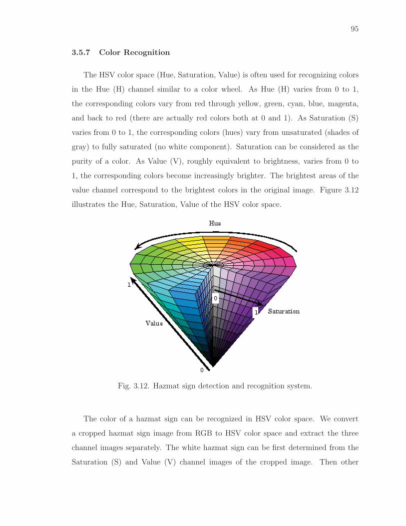
95
3.5.7 Color Recognition
The HSV color space (Hue, Saturation, Value) is often used for recognizing colors
in the Hue (H) channel similar to a color wheel. As Hue (H) varies from 0 to 1,
the corresponding colors vary from red through yellow, green, cyan, blue, magenta,
and back to red (there are actually red colors both at 0 and 1). As Saturation (S)
varies from 0 to 1, the corresponding colors (hues) vary from unsaturated (shades of
gray) to fully saturated (no white component). Saturation can be considered as the
purity of a color. As Value (V), roughly equivalent to brightness, varies from 0 to
1, the corresponding colors become increasingly brighter. The brightest areas of the
value channel correspond to the brightest colors in the original image. Figure 3.12
illustrates the Hue, Saturation, Value of the HSV color space.
Fig. 3.12. Hazmat sign detection and recognition system.
The color of a hazmat sign can be recognized in HSV color space. We convert
a cropped hazmat sign image from RGB to HSV color space and extract the three
channel images separately. The white hazmat sign can be first determined from the
Saturation (S) and Value (V) channel images of the cropped image. Then other

96
Table 3.2The color look-up table based on the 32 uniform distributed hue segments.
Recognized Colors Red(1) Orange Yellow Green Blue Red(2)
Hue Segment Range 0∼0.03125 0.03125∼0.09375 0.09375∼0.25 0.25∼0.5 0.5∼0.75 0.75∼1
Hue Segment Indexes 1 2,3 4∼8 9∼16 17∼24 25∼32
colorful hazmat sign can be recognized from the masked regions of the Hue (H)
channel image of the cropped image. This can be done by an image masking method
using image thresholding on saturation and value channel images because white’s
saturation is close to 0 and its value is close to 1. We compute the histograms of the
saturation and value channel images of the cropped image and then employ the Otsu’s
thresholding method [121] to binarize the channel images and obtain two masks of
resultant regions whose saturation and value are greater than their thresholds. A
combined mask is obtained by AND operations of saturation and value masks and it
denotes the mask of color regions in the cropped image since the Saturation (S) and
Value (V) channels are both orthogonal to the Hue (H) channel. The masked color
regions is used to check if the hazmat sign is white or other color. A hazmat sign is
considered as white if the size of the masked color regions is less than 0.4% of the
number of pixels in the cropped image, otherwise it is considered as other color in
the following.
To determine the color (except white) of the masked color regions, we first define
a set of K uniform distributed hue segments by equally dividing the whole range of
the hue channel (from 0 to 1). A histogram of K bins of the hue segments is used to
characterize the hue distribution of the cropped hazmat sign image. We find the index
Bk of the maximum number of pixel counts in the histogram and use it to determine
the color (except white) of the hazmat sign by searching Bk in an empirically obtained
color look-up table in Table 3.2 based on the K bins of the hue segments. The size
of look-up table is determined by the number of hue segments K and we use K = 32
in our color recognition method. Some examples of the proposed color recognition

97
method for white and colorful hazmat signs at 50 feet are illustrated from Figure 3.13
to Figure 3.16 respectively (The hazmat sign images with 4-digit UNID were captured
by 5 MP camera on an HTC Wildfire mobile telephone (2592×1952) and the ones
with warning text were captured by a 5 MP camera on a Samsung Galaxy Nexus
mobile telephone (2592×1944)). The recognized color is used for queuing the mobile
database for sign category identification and providing the general guide information
based on the 2012 ERG guidebook.

98
Fig. 3.13. Examples of the proposed color recognition method for twowhite hazmat signs at 50 feet.
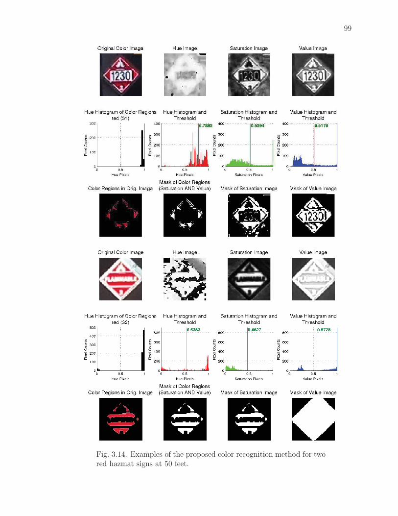
99
Fig. 3.14. Examples of the proposed color recognition method for twored hazmat signs at 50 feet.
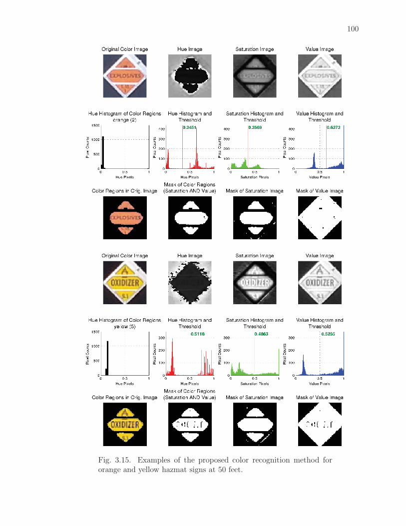
100
Fig. 3.15. Examples of the proposed color recognition method fororange and yellow hazmat signs at 50 feet.

101
Fig. 3.16. Examples of the proposed color recognition method forgreen and blue hazmat signs at 50 feet.
102
3.6 Experimental Results
We did two experiments to investigate the performance and accuracy of our pro-
posed hazmat sign detection and recognition method. The tests were executed on a
Galaxy Nexus mobile telephone with a dual-core 1.2GHz CPU and 1GB RAM and
a backend server with a quad-core 2.4GHz CPU and 4GB RAM. The first experi-
ment consisted of generating saliency maps using different visual saliency models and
evaluating their performance of locating hazmat signs based on ground-truth infor-
mation. The second experiment consisted of hazmat sign detection and recognition
on our image datasets and comparing the results with ground-truth information. The
ground-truth information include the image resolution, the number of pixels on the
sign, the distance from the camera to the sign, sign color, and sign location in the
image.
3.6.1 Image Datasets
Our first image dataset (Dataset-1) consisted of 50 images, each containing one or
more hazmat signs in a complex scene (62 hazmat signs in total). The hazmat sign
images were captured by a third party under various lighting conditions, distances
and perspectives using three different cameras: a 5 MP camera on an HTC Wildfire
mobile telephone (2592×1952), an 8.2 MP Kodak Easyshare C813 digital camera
(3296×2472), and a 16 MP Nikon Coolpix S800c digital camera (1600×1200) (MP
stands for Mega Pixel). Among the 50 images, 23 were reported at 10-50 feet, 23 at
50-100 feet, and 4 at 100-150 feet. Among the 62 hazmat signs, 2 had low resolution,
11 had projective distortion, 8 were blurred, and 6 were shaded. This image dataset
contains images of red, yellow, and white hazmat signs. Figure 3.17 illustrates some
examples of the first image dataset (Dataset-1) in different conditions.
Our second image dataset (Dataset-2) consisted of 100 images, each containing one
or more hazmat signs in a complex scene (111 hazmat signs in total). The hazmat sign
images were captured by a third party under various lighting conditions, distances

103
Fig. 3.17. Examples of the first image dataset (Dataset-1) in differentconditions (left to right then top to bottom): low resolution, perspec-tive distortion; blurred sign, shaded sign.
and perspectives using the 16 MP Nikon Coolpix S800c digital camera, including
36 low resolution 2 MP images (1600×1200) and 64 full resolution 16 MP images
(4608×3456) from the same camera. Among the 100 images, 22 were reported at 10-
50 feet, 35 at 50-100 feet, and 43 at 100-150 feet. Among the 111 hazmat signs, 46 had
low resolution, 25 had projective distortion, 12 were blurred, and 17 were shaded. This
image dataset contains images of red and white hazmat signs. Figure 3.18 illustrates
some examples of the second image dataset (Dataset-2) in different conditions.
Our third image dataset (Dataset-3) consisted of 252 images, each containing only
one hazmat sign in a complex scene (252 hazmat signs in total). We use 6 available
hazmat signs in different colors for this image dataset, including red, green, blue,
orange, yellow, and white. All of them have a warning text in the middle of the signs

104
Fig. 3.18. Examples of the second image dataset (Dataset-2) in dif-ferent conditions (left to right then top to bottom): low resolution,perspective distortion; blurred sign, shaded sign.
often used by truck trailer. The images were acquired by us in the outdoor field under
various lighting conditions and distances. We took the images at various distances
with ground-truth measurement, i.e. 10, 25, 50, 75, 100, 125, and 150 feet. The
hazmat sign images were captured by us using 3 different cameras: a 5 MP camera
on an HTC Wildfire mobile telephone (2592×1952), a 5 MP camera on a Samsung
Galaxy Nexus mobile telephone (2592×1944), and a 10 MP Canon PowerShot S95
digital camera (3648×2736) (MP stands for Mega Pixel). At each distance, 36 images
were taken by the 3 cameras in both portrait mode and landscape mode (12 images
of the 6 hazmat signs in each scene). Among the 252 images, 36 were measured and
captured in a straight view at 10 feet, 36 at 25 feet, 36 at 50 feet, 36 at 75 feet,
36 at 100 feet, 36 at 125 feet, and 36 at 150 feet. The 252 hazmat signs have clear
appearances without any shape distortion in the images. This image dataset contains
images of red, green, blue, orange, yellow, and white hazmat signs. Figure 3.19 and
Figure 3.20 illustrate some examples of the 6 signs of the third image dataset (Dataset-

105
3) at 10 feet in portrait an landscape mode respectively (Images were captured by
the 5 MP camera on a Samsung Galaxy Nexus mobile telephone).
The distance information of the first and second image datasets (Dataset-1 and
Dataset-2) is visually estimated and thus not reliable. The images were also acquired
by a third party in the working field, under various lighting and weather conditions,
distances, and perspectives. The distance information of the third image dataset
(Dataset-3) is reliable and obtained with ground-truth measurement. The images
were acquired by us in the outdoor field under various lighting conditions and dis-
tances.
Fig. 3.19. Examples of the 6 signs of Dataset-3 at 10 feet in portraitmode (left to right then top to bottom): red sign, green sign, bluesign; orange sign, yellow sign, white sign.

106
Fig. 3.20. Examples of the 6 signs of Dataset-3 at 10 feet in landscapemode (left to right then top to bottom): red sign, green sign, blue sign;orange sign, yellow sign, white sign.

107
Figure 3.21 illustrate some bounding box images for a typical STOP sign and a
hazmat sign at the same distance 25, 50, 100, and 150 feet. Table 3.3 shows the
relation among the image resolution of a certain camera, the distance from a camera
to a hazmat sign, and the number of pixels on a hazmat sign. It also reports the
pixel ratio of STOP and hazmat sign by comparing it to a typical STOP sign at each
distance. On average, a typical STOP sign contains 5.60 times pixels than a hazmat
sign at the same distance.
Fig. 3.21. Examples of bounding box images for a typical STOP signand a hazmat sign at the same distance 25, 50, 100, and 150 feet.

108
Table 3.3The relation among the image resolution, the distance from a camera to a hazmat sign, and the number ofpixels on a hazmat sign in the third image dataset (Dataset-3) with comparison to a typical STOP sign.
Camera (Image Resolution) 10 feet 25 feet 50 feet 75 feet 100 feet 125 feet 150 feet
Canon PowerShot S95 (3648×2736) 90312 14450 3444 1458 840 512 364
Hazmat Sign Bounding Box (Pixel Ratio=0.5) 425×425 170×170 83×83 54×54 41×41 32×32 27×27
HTC Wildfire (2592×1952) 57800 9522 2312 1012 578 364 242
Hazmat Sign Bounding Box (Pixel Ratio=0.5) 340×340 138×138 68×68 45×45 34×34 27×27 22×22
Samsung Galaxy Nexus (2592×1944) 56112 9248 2244 1012 578 364 242
Hazmat Sign Bounding Box (Pixel Ratio=0.5) 335×335 136×136 67×67 45×45 34×34 27×27 22×22
Samsung Galaxy Nexus (2592×1944) 298235 50952 12738 5845 3288 1989 1393
STOP Sign Bounding Box (Pixel Ratio=0.82843) 600×600 248×248 124×124 84×84 63×63 49×49 41×41
Pixel Ratio of STOP and Hazmat Sign (Avg=5.60) 5.315 5.510 5.676 5.776 5.689 5.464 5.756

109
3.6.2 The First Experiment
In the first experiment, we tested our best GCS visual saliency models and 4
state-of-the-art models, including SBVA [25], GBVS [26], IS-DCT-Lab [33], SSA-
HFT-IRGBY [35], by hazmat sign image dataset. This experiment consisted of eval-
uating their performance using a hazmat sign image dataset and scoring the resultant
saliency maps in locating hazmat signs based on ground-truth information. We use
the first hazmat sign image dataset (Dataset-1) for evaluation and it consists of 50
images and 62 hazmat signs in total.
The saliency models are evaluated in the experiment are: SBVA [25], GBVS [26],
IS [33], SSA [35]. We classified the resulting saliency maps into four categories:
good, fair, bad, and lost. For each sign, we assigned 3 points for a good saliency
map (sign was mostly contained in high salient regions SRhigh), 2 points for a fair
saliency map (sign was mostly contained in middle salient regions SRmiddle), 1 point
for a bad saliency map (sign was mostly contained in low salient regions SRlow),
and 0 points for a lost saliency map (sign was mostly contained in non-salient regions
SRnon). The type of salient regions are distinguished by a set of predefined thresholds
(The multiples of the average saliency value of a given saliency map based on the
Equation 3.2).
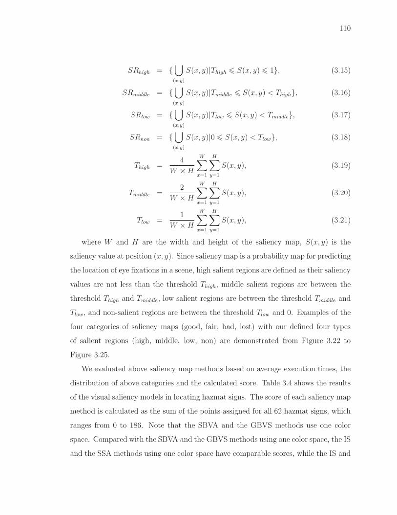
110
SRhigh = {⋃(x,y)
S(x, y)|Thigh � S(x, y) � 1}, (3.15)
SRmiddle = {⋃(x,y)
S(x, y)|Tmiddle � S(x, y) < Thigh}, (3.16)
SRlow = {⋃(x,y)
S(x, y)|Tlow � S(x, y) < Tmiddle}, (3.17)
SRnon = {⋃(x,y)
S(x, y)|0 � S(x, y) < Tlow}, (3.18)
Thigh =4
W ×H
W∑x=1
H∑y=1
S(x, y), (3.19)
Tmiddle =2
W ×H
W∑x=1
H∑y=1
S(x, y), (3.20)
Tlow =1
W ×H
W∑x=1
H∑y=1
S(x, y), (3.21)
where W and H are the width and height of the saliency map, S(x, y) is the
saliency value at position (x, y). Since saliency map is a probability map for predicting
the location of eye fixations in a scene, high salient regions are defined as their saliency
values are not less than the threshold Thigh, middle salient regions are between the
threshold Thigh and Tmiddle, low salient regions are between the threshold Tmiddle and
Tlow, and non-salient regions are between the threshold Tlow and 0. Examples of the
four categories of saliency maps (good, fair, bad, lost) with our defined four types
of salient regions (high, middle, low, non) are demonstrated from Figure 3.22 to
Figure 3.25.
We evaluated above saliency map methods based on average execution times, the
distribution of above categories and the calculated score. Table 3.4 shows the results
of the visual saliency models in locating hazmat signs. The score of each saliency map
method is calculated as the sum of the points assigned for all 62 hazmat signs, which
ranges from 0 to 186. Note that the SBVA and the GBVS methods use one color
space. Compared with the SBVA and the GBVS methods using one color space, the IS
and the SSA methods using one color space have comparable scores, while the IS and

111
Table 3.4Average execution time (in seconds), distribution and score of thesaliency models (color spaces) in the first image dataset (Dataset-1).
Saliency Map Time Good Fair Bad Lost Score
SBVA(IRGBY) 2.07 28 16 12 6 128
GBVS(IRGBY) 3.36 25 15 15 7 120
IS(Lab) 0.39 27 5 20 10 111
IS(RGB) 0.36 22 7 27 6 107
SSA(Lab) 0.55 33 8 12 9 127
SSA(RGB) 0.53 38 5 8 11 132
IS+SSA(Lab+RGB) 1.83 41 6 8 7 143
GCS(Lab) 0.43 37 10 8 7 139
GCS(RGB) 0.41 28 16 12 6 128
GCS(Lab+RGB) 0.84 52 6 1 3 169

112
Fig. 3.22. An example of good saliency map with the four types ofsalient regions (top to bottom then left to right): original image, goodsaliency map; high salient regions, middle salient regions; low salientregions, non-salient regions.
the SSA methods using two color spaces have higher scores. The GCS(Lab+RGB)
and the IS+SSA(Lab+RGB) methods using two color spaces run 2.46 and 1.13 times
faster than the SBVA method and 4.0 and 1.84 times faster than the GBVS method
respectively. The results verified that the proposed GCS(Lab+RGB) model, com-
bining GCS-FT-Lab and GCS-FT-RGB models, can improve the score of generated

113
Fig. 3.23. An example of fair saliency map with the four types ofsalient regions (top to bottom then left to right): original image, fairsaliency map; high salient regions, middle salient regions; low salientregions, non-salient regions.
saliency maps, while still running faster than SBVA and GBVS methods. Figure 3.26
and Figure 3.27 illustrate examples of saliency maps from different methods for the
same hazmat sign images in portrait mode and landscape mode. Note that the table
in the middle indicates the locations of the saliency maps corresponding to which
methods.

114
Fig. 3.24. An example of bad saliency map with the four types ofsalient regions (top to bottom then left to right): original image, badsaliency map; high salient regions, middle salient regions; low salientregions, non-salient regions.

115
Fig. 3.25. An example of lost saliency map with the four types ofsalient regions (top to bottom then left to right): original image, lostsaliency map; high salient regions, middle salient regions; low salientregions, non-salient regions.
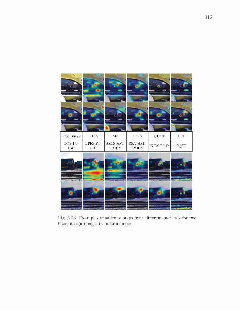
116
Fig. 3.26. Examples of saliency maps from different methods for twohazmat sign images in portrait mode.

117
Fig. 3.27. Examples of saliency maps from different methods for twohazmat sign images in landscape mode.
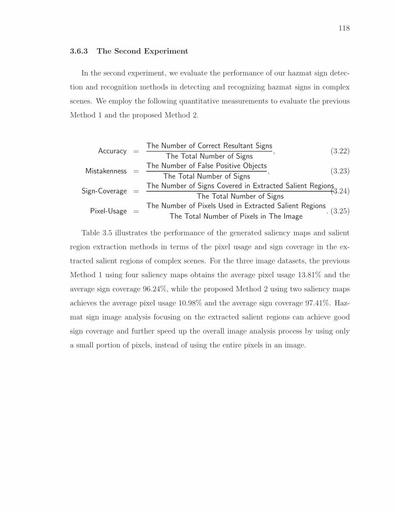
118
3.6.3 The Second Experiment
In the second experiment, we evaluate the performance of our hazmat sign detec-
tion and recognition methods in detecting and recognizing hazmat signs in complex
scenes. We employ the following quantitative measurements to evaluate the previous
Method 1 and the proposed Method 2.
Accuracy =The Number of Correct Resultant Signs
The Total Number of Signs, (3.22)
Mistakenness =The Number of False Positive Objects
The Total Number of Signs, (3.23)
Sign-Coverage =The Number of Signs Covered in Extracted Salient Regions
The Total Number of Signs,(3.24)
Pixel-Usage =The Number of Pixels Used in Extracted Salient Regions
The Total Number of Pixels in The Image. (3.25)
Table 3.5 illustrates the performance of the generated saliency maps and salient
region extraction methods in terms of the pixel usage and sign coverage in the ex-
tracted salient regions of complex scenes. For the three image datasets, the previous
Method 1 using four saliency maps obtains the average pixel usage 13.81% and the
average sign coverage 96.24%, while the proposed Method 2 using two saliency maps
achieves the average pixel usage 10.98% and the average sign coverage 97.41%. Haz-
mat sign image analysis focusing on the extracted salient regions can achieve good
sign coverage and further speed up the overall image analysis process by using only
a small portion of pixels, instead of using the entire pixels in an image.

119
Table 3.5The pixel usage and sign coverage in the extracted salient regions for the three image datasets.
Dataset-1 Dataset-1 Dataset-2 Dataset-2 Dataset-3 Dataset-3 Average Average
Proposed Method Pixel Usage Sign Coverage Pixel Usage Sign Coverage Pixel Usage Sign Coverage Pixel Usage Sign Coverage
IS+SSA(Lab+RGB) Sal. Maps 15.29% 98.39%(61/62) 14.63% 95.50%(106/111) 11.52% 96.03%(242/252) 13.81% 96.24%(409/425)
GCS(Lab+RGB) Sal. Maps 12.52% 98.39%(61/62) 11.73% 96.40%(107/111) 8.70% 97.62%(246/252) 10.98% 97.41%(414/425)
120
The accuracy of sign location detection is significantly related to the image res-
olution of a certain camera, the distance from a camera to a hazmat sign, and the
number of pixels on a hazmat sign. We then determine the color recognition accuracy
based on how many signs were correctly color recognized after a successful sign loca-
tion detection. Note that we used the recognized color inside the sign, not text or UN
identifier numbers, queuing the mobile database for sign category identification and
providing the general guide information. Therefore the overall accuracy is equivalent
to the color recognition accuracy in our experiments.
Table 3.6 illustrates the image analysis results of the proposed methods for the first
image dataset (Dataset-1). The previous Method 1 using the IS+SSA(Lab+RGB)
model has the location detection accuracy 64.52% and the color recognition accuracy
45.16% for all 62 hazmat signs. The proposed Method 2 using our GCS(Lab+RGB)
model obtains the location detection accuracy 67.74% and the color recognition ac-
curacy 61.29%, while the same method without using saliency maps yields 56.45%
and 50.00% respectively. Table 3.7 demonstrates the image analysis results of the
proposed methods for the second image dataset (Dataset-2). The previous Method
1 using the IS+SSA(Lab+RGB) model has the location detection accuracy 40.54%
and the color recognition accuracy 29.73% for all 111 hazmat signs. The proposed
Method 2 using our GCS(Lab+RGB) model obtain the location detection accuracy
54.05% and the color recognition accuracy 53.15%, while the same method without
using saliency maps yields 43.24% and 42.34% respectively. Compared with our pre-
vious Method 1 using the IS+SSA(Lab+RGB) model with four saliency maps, our
proposed Method 2 using our GCS(Lab+RGB) model with two saliency maps has
higher accuracy of sign location detection in general. Our experimental results con-
firmed that the proposed visual saliency based image analysis methods can increase
the accuracy of sign location detection and reduce the false positive (FP) objects.
For our third image dataset (Dataset-3), Table 3.8, Table 3.9 and Table 3.10 show
more image analysis results of the proposed methods at variant distances for the third
image dataset (Dataset-3), including the mistakenness of false positive (FP) objects,

121
Table 3.6Image analysis results for the first image dataset (Dataset-1).
Total FP Object FP Object Location Location Color Color Overall
Proposed Method Signs Extracted Mistakenness Detected Accuracy Recognized Accuracy Accuracy
Method 1 IS+SSA(Lab+RGB) Sal. Maps 62 10 16.13% 40 64.52% 28 45.16% 45.16%
Method 2 without Sal. Maps 62 32 51.61% 35 56.45% 31 50.00% 50.00%
Method 2 GCS(Lab+RGB) Sal. Maps 62 21 33.87% 42 67.74% 38 61.29% 61.29%

122
Table 3.7Image analysis results for the second image dataset (Dataset-2).
Total FP Object FP Object Location Location Color Color Overall
Proposed Method Signs Extracted Mistakenness Detected Accuracy Recognized Accuracy Accuracy
Method 1 IS+SSA(Lab+RGB) Sal. Maps 111 24 21.62% 45 40.54% 33 29.73% 29.73%
Method 2 without Sal. Maps 111 81 72.97% 48 43.24% 47 42.34% 42.34%
Method 2 GCS(Lab+RGB) Sal. Maps 111 45 40.54% 60 54.05% 59 53.15% 53.15%
123
the location detection accuracy, the color recognition accuracy, and the overall process
accuracy. The previous Method 1 using the IS+SSA(Lab+RGB) model has the av-
erage location detection accuracy 56.75% and the average color recognition accuracy
19.05% for all 252 hazmat signs. The proposed Method 2 using our GCS(Lab+RGB)
model achieves the average location detection accuracy 96.83% and the average color
recognition accuracy 90.87%, while the same method using saliency maps obtains
87.70% and 82.54% respectively. The previous Method 1 has high location accuracy
at short distances but decreases after 50 feet and fails to detect sign location after
125 feet. The proposed Method 2 achieve relatively consistent location accuracy at
all distances from 10 feet to 150 feet, because we used the adaptive contour extrac-
tion method within more accurate saliency regions and the robust contour matching
method based on Fourier descriptors.
For the overall process of our hazmat sign image analysis system, the average
execution time of the previous Method 1 and the one of the proposed Method 2
are 5.88 and 5.28 seconds respectively for the first image dataset (Dataset-1), 18.95
and 16.45 seconds respectively for the second image dataset (Dataset-2), while 10.24
and 8.98 seconds respectively for the third image dataset (Dataset-3). The average
execution time of the proposed Method 2 without using saliency maps are 8.49, 26.52,
and 14.36 seconds for the three image datasets respectively. Our experimental results
verified that the proposed visual saliency based methods can speed up the overall
image analysis process. With better location detection accuracy and color recognition
accuracy, the proposed Method 2 using the GCS(Lab+RGB) model is faster than
the previous Method 1 using the IS+SSA(Lab+RGB) model and more suitable for
practical applications and uses.

124
Table 3.8Image analysis results of Method 1 using four saliency maps for the third image dataset (Dataset-3).
Method 1 Total FP Object FP Object Location Location Color Color Overall
IS+SSA(Lab+RGB) Sal. Maps Signs Extracted Mistakenness Detected Accuracy Recognized Accuracy Accuracy
10 feet 36 8 22.22% 36 100.00% 10 27.78% 27.78%
25 feet 36 4 11.11% 36 100.00% 16 44.44% 44.44%
50 feet 36 2 5.56% 34 94.44% 10 27.78% 27.78%
75 feet 36 1 2.78% 23 63.89% 7 19.44% 19.44%
100 feet 36 1 2.78% 11 30.56% 3 8.33% 8.33%
125 feet 36 4 11.11% 3 8.33% 2 5.56% 5.56%
150 feet 36 4 11.11% 0 0.00% 0 0.00% 0.00%
Average 252 24 9.52% 143 56.75% 48 19.05% 19.05%

125
Table 3.9Image analysis results of Method 2 without using saliency maps for the third image dataset (Dataset-3).
Method 2 Total FP Object FP Object Location Location Color Color Overall
without using Sal. Maps Signs Extracted Mistakenness Detected Accuracy Recognized Accuracy Accuracy
10 feet 36 4 11.11% 33 91.67% 29 80.56% 80.56%
25 feet 36 50 138.89% 26 72.22% 26 72.22% 72.22%
50 feet 36 3 8.33% 34 94.44% 33 91.67% 91.67%
75 feet 36 5 13.89% 32 88.89% 30 83.33% 83.33%
100 feet 36 3 8.33% 34 94.44% 32 88.89% 88.89%
125 feet 36 9 25.00% 30 83.33% 28 77.78% 77.78%
150 feet 36 3 8.33% 32 88.89% 30 83.33% 83.33%
Average 252 77 30.56% 221 87.70% 208 82.54% 82.54%

126
Table 3.10Image analysis results of Method 2 using two saliency maps for the third image dataset (Dataset-3).
Method 2 Total FP Object FP Object Location Location Color Color Overall
GCS(Lab+RGB) Sal. Maps Signs Extracted Mistakenness Detected Accuracy Recognized Accuracy Accuracy
10 feet 36 0 0.00% 36 100.00% 32 88.89% 88.89%
25 feet 36 1 2.78% 36 100.00% 36 100.00% 100.00%
50 feet 36 0 0.00% 36 100.00% 35 97.22% 97.22%
75 feet 36 1 2.78% 36 100.00% 34 94.44% 94.44%
100 feet 36 7 19.44% 33 91.67% 31 86.11% 86.11%
125 feet 36 20 55.56% 33 91.67% 30 83.33% 83.33%
150 feet 36 19 52.78% 34 94.44% 31 86.11% 86.11%
Average 252 48 19.05% 244 96.83% 229 90.87% 90.87%

127
Discussion
¿From the experiments our accuracy ranged from approximately 90% for images
taken is a controlled test environment to approximately 60% for image acquired in
a more “typical” operating scenario. The accuracy we obtained in a more typical
operating scenario would not be acceptable for many situations. The overall accu-
racy of our hazmat sign image analysis system is affected by the location and color
recognition accuracy. The accuracy of sign location detection is significantly related
to the image resolution of the camera, the distance from the camera to a hazmat sign,
and the number of pixels forming the hazmat sign. As mentioned above, we show the
relation between these factors in Table 3.3. The location detection accuracy of the
first Dataset-1 67.74% and the second Dataset-2 54.05% were lower than the average
one of the third Dataset-3 96.83%, because there are a large number of blurred, low
resolution, and perspective distorted hazmat signs contained in the first Dataset-1
and the second Dataset-2. Note that hazmat signs in the third Dataset-3 were ac-
quired in a controlled test environment without any shape distortion in the images.
The location detection accuracy deteriorates due to the loss of boundary contours for
blurred and low resolution hazmat signs and poor correlation in contour matching for
perspective distorted hazmat signs.
The color recognition accuracy is based on how many signs were correctly color
recognized after a successful sign location detection. The color recognition accuracy of
the first Dataset-1 61.29% and the second Dataset-2 53.15% were also lower than the
average one of the third Dataset-3 90.87%, because the color recognition accuracy will
not exceed the previous location detection accuracy. The color recognition accuracy
is also degraded by the absence of color calibration for hazmat sign images, especially
for shaded signs, which cause our color recognition method to misidentify the sign
color.
The location detection accuracy could be improved by using supper-resolution
image reconstruction methods [126, 127] to refine hazmat sign images at the step of

128
image preprocessing. The color recognition accuracy could be increased by employing
proper color calibration methods [51] at the step of image acquisition. Therefore we
could further improve the overall accuracy of our hazmat sign image analysis system.

129
4. ERROR CONCEALMENT FOR
SCALABLE VIDEO CODING
A Scalable video coding (SVC) decoder typically requires that the base layer frames
be delivered almost error-free and uses them to decode the enhancement layer frames.
Due to the nature of dynamic and lossy channels used for video delivery (particularly
wireless channels), video bitstreams transmitted over packet networks usually expe-
rience isolated and burst packet losses [17]. An accurate distortion model for the
effect of different packet loss patterns on the encoded video was proposed in [128]. It
confirmed that a burst packet loss produces a larger distortion than an equal number
of isolated packet losses. Moreover, once errors occur in video bitstreams, they are
prone to propagate from one frame to another due to motion-compensated prediction
used in SVC codec. These effects can result in severe visual quality degradation of
the decoded frames.
Error concealment (EC) is an effective scheme for error recovery, which imposes
small complexity on the decoder and provides a flexible solution to the above prob-
lems [129, 130]. By the use of error concealment methods, damaged regions can be
reconstructed from the correctly received neighboring regions. Due to the layered
structure of SVC, it is advantageous to recover the damaged frames in one layer us-
ing the available frames in other layers. It has been shown that one can exploit the
spatial and temporal correlations of video frames between different layers to improve
the performance of single layer error concealment [18].
Slice structuring [130] is a useful strategy to reduce error propagation from a
damaged slice/packet to subsequent slices/packets from burst packet losses. Slice
interleaving (SI) [131] and flexible macroblock ordering (FMO) [132] are two com-
mon slice structuring schemes. Interleaving approach has been exploited for slice
130
structuring and packetization. A near-optimal packet interleaving method was pro-
posed in [133] based on an optimization criteria in terms of temporal neighbor packet
distance. Another packetization method was introduced in [134] based on optimal
packetization masks, which aims to simultaneously maximize the intra-partition dis-
tance and distribute neighboring coefficients equally among different packets. The
FMO technique has been employed to independently assign each macroblock (MB)
of a frame to a certain slice group (SG) by a macroblock allocation map (MBAmap).
The H.264/AVC video coding standard specifies seven types of FMO to support error
resilience [132]. FMO Type 1 is also known as scattered or dispersed slices. The
effect of error propagation between frames has been investigated in [135] and a more
suitable MBAmap with a reduced effect of error propagation can be generated based
on the evaluation of each macroblock’s importance. In [136], an adaptive MBAmap
updating scheme is proposed to reduce the computational cost of FMO and a slice
matching error concealment method is also introduced. In [137], a new FMO method
was proposed by solving an optimization problem of optimal MB labeling for burst
packet loss resilience.
In this chapter, a two-layer spatial-temporal SVC system is developed for inter-
layer error concealment. The enhancement layer has high spatial resolution at high
frame rate (e.g. 30 fps) and the base layer has low resolution at low frame rate (e.g.
15 fps). It is assumed that the packet delivery of the base layer is loss-prone the
same way as the enhancement layer. In this scenario, three inter-layer error conceal-
ment methods are proposed using two new approaches. (1) Motion vector averaging
using adaptively averaging over multiple types of motion vectors in different layers
for the recovery of lost motion vectors. (2) Slice interleaving utilizing an optimum
ordering technique to make the average distance between two contiguous slices as far
as possible. The proposed error concealment method is capable of decoding the SVC
bitstreams under burst packet losses and reconstructing the damaged frames with
enhanced visual quality. The effect of burst packet losses and error propagation on

131
video frames in both layers is investigated regarding two existing and three proposed
error concealment methods.
4.1 Error Concealment Methods
4.1.1 Conventional Error Concealment Methods
The SVC reference codec, Joint Scalable Video Model (JSVM), introduced four
non-normative error concealment (EC) methods [138] to address the problem of error
recovery. (1) Picture copy (PC): Each pixel value of the concealed frame is copied
from the corresponding pixel of the first frame in the reference frame list 0. (2)
Temporal direct motion vector generation (TD): This predicts a missing frame using
two reference frame lists and generates the desired missing motion vectors by scaling
the motion vectors inferred from its neighboring reference frames. (3) Motion and
residual upsampling or base layer skip (BLSkip): This conceals a lost enhancement
layer frame from the predicted P- or B-frames. The residuals and motion vectors of
the base layer will be up-sampled to higher resolution for the enhancement layer. (4)
Reconstruction base layer upsampling (RU): The base layer frame is reconstructed
and up-sampled using a 6-tap H.264/AVC filter for the lost enhancement layer frame.
In addition, a new intra-layer method was introduced in [18]. (5) Motion copy (MC):
The reconstruction of the last key frame is re-used as the reference. Motion vectors
are re-generated by copying the motion field of the last key frame. Single-layer EC
methods include FC, TD and MC, while inter-layer EC methods include BLSkip and
RU. The experimental results in [18] concluded that the BLSkip-based method is a
desirable SVC EC tool.
4.1.2 Related Work
Motion vector error concealment has been an active research area for many years.
A block-based motion vector extrapolation (MVE) method was proposed in [139].

132
Some MVs of correlated MBs in the previous frame are first extrapolated to the
current damaged frame and then the lost MV of the damaged MB is replaced by the
best MV of the motion extrapolated MB with the largest overlapped area. A pixel-
based MVE (PMVE) method was introduced [140] by extending the block-based
MVE method [139] to the pixel level. A hybrid MVE (HMVE) scheme was proposed
in [141] based on the pixel-based and block-based MVE, which is able to discard the
wrongly extrapolated MVs in order to obtain more accurate MV. In [142], a block-
based motion projection (MP) approach was proposed to reconstruct the lost MV of
the damaged block based on its qualified temporal blocks’ MVs and spatial neighbors’
MVs. In general, block-based MVE and MP methods are similar in terms of that
they all used MVs from the projected blocks in previous frame and select the best
MV of the block with the largest overlapped area. But MP employs a post-processing
stage and median filtering is capable of refining the reconstructed MV field.
The visual quality of the error concealed regions can be further improved with
the help of slice interleaving. It is aimed at spreading contiguous slices over different
packets against packet losses, so that damaged regions can be surrounded by some cor-
rectly received regions. A simple slice interleaving approach was used in [131], where
each slice consists of disjoint single lines of macroblocks in a frame. In [128], a packet
interleaver was presented to interleave the packets before transmission and cope with
burst packet losses, where packets are first loaded into the block interleaver in rows
and are transmitted by columns. A distance-based slice interleaving method [143]
was proposed to rearrange independently decodable slices of consecutive frames into
packets according to an optimal interleaving structure for packetization. Each slice is
interleaved by achieving the maximum minimal distance between contiguous slices.
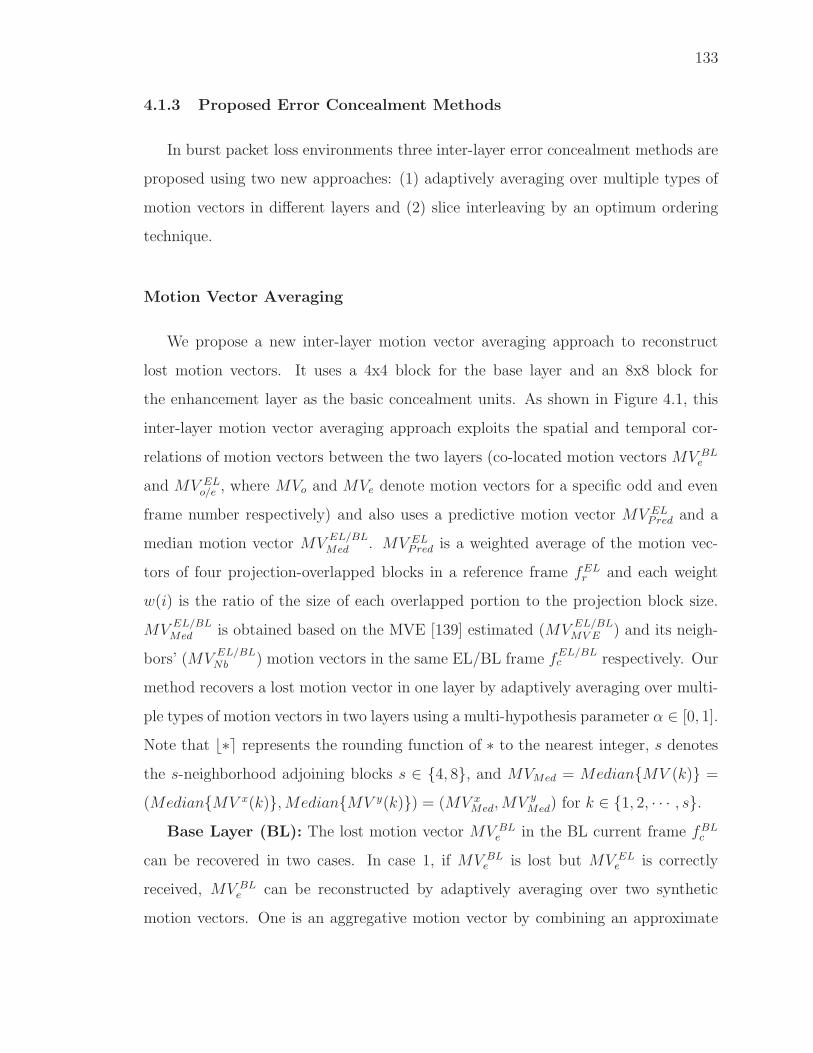
133
4.1.3 Proposed Error Concealment Methods
In burst packet loss environments three inter-layer error concealment methods are
proposed using two new approaches: (1) adaptively averaging over multiple types of
motion vectors in different layers and (2) slice interleaving by an optimum ordering
technique.
Motion Vector Averaging
We propose a new inter-layer motion vector averaging approach to reconstruct
lost motion vectors. It uses a 4x4 block for the base layer and an 8x8 block for
the enhancement layer as the basic concealment units. As shown in Figure 4.1, this
inter-layer motion vector averaging approach exploits the spatial and temporal cor-
relations of motion vectors between the two layers (co-located motion vectors MV BLe
and MV ELo/e , where MVo and MVe denote motion vectors for a specific odd and even
frame number respectively) and also uses a predictive motion vector MV ELPred and a
median motion vector MVEL/BLMed . MV EL
Pred is a weighted average of the motion vec-
tors of four projection-overlapped blocks in a reference frame fELr and each weight
w(i) is the ratio of the size of each overlapped portion to the projection block size.
MVEL/BLMed is obtained based on the MVE [139] estimated (MV
EL/BLMV E ) and its neigh-
bors’ (MVEL/BLNb ) motion vectors in the same EL/BL frame f
EL/BLc respectively. Our
method recovers a lost motion vector in one layer by adaptively averaging over multi-
ple types of motion vectors in two layers using a multi-hypothesis parameter α ∈ [0, 1].
Note that �∗ represents the rounding function of ∗ to the nearest integer, s denotes
the s-neighborhood adjoining blocks s ∈ {4, 8}, and MVMed = Median{MV (k)} =
(Median{MV x(k)},Median{MV y(k)}) = (MV xMed,MV y
Med) for k ∈ {1, 2, · · · , s}.Base Layer (BL): The lost motion vector MV BL
e in the BL current frame fBLc
can be recovered in two cases. In case 1, if MV BLe is lost but MV EL
e is correctly
received, MV BLe can be reconstructed by adaptively averaging over two synthetic
motion vectors. One is an aggregative motion vector by combining an approximate

134
Fig. 4.1. The proposed inter-layer motion vector averaging approachusing adaptively averaging over multiple types of motion vectors intwo layers.
motion vector 12MV EL
e in the EL corresponding frame fELc and a predictive motion
vector 12MV EL
Pred in the EL reference frame fELr . The other is a median motion vector
MV BLMed based on the MVE estimated and s neighbors’ motion vectors in the same
BL frame. In case 2, if MV ELe and MV BL
e are both lost, MV BLe can be reconstructed
using the median median motion vector MV BLMed in the same BL frame.
BL Case 1: If MV BLe is lost but MV EL
e is correctly received,
MV BLe = �α(1
2MV EL
e +1
2MV EL
Pred) + (1− α)MV BLMed , (4.1)
MV ELPred =
∑i
w(i) ∗MV ELo (i)/
∑i
w(i), (4.2)
MV BLMed = Median{MV BL
MV E
⋃MV BL
Nb (k)}. (4.3)
BL Case 2: If MV BLe and MV EL
e are both lost,
MV BLe = MV BL
Med. (4.4)

135
Enhancement Layer (EL): The lost motion vector MV ELo/e in the EL current
frame fELc can be reconstructed in two cases, where MV EL
o/e denotes either MV ELo
or MV ELe for a specific odd or even frame number. In case 1, if MV EL
o/e is lost but
MV BLe is correctly received, MV EL
o/e can be recovered by adaptively averaging over two
synthetic motion vectors. One is an approximate motion vector 2∗ 12MV BL
e = MV BLe
in BL corresponding frame fBLc . The other is a median motion vector MV EL
o/e,Med based
on the MVE estimated and s neighbors’ motion vectors in the same EL odd/even
frame. In case 2, if MV BLe and MV EL
o/e are both lost, MV ELo/e can be recovered using
the median motion vector MV ELo/e,Med in the same EL odd/even frame.
EL Case 1: If MV ELo/e is lost but MV BL
e is correctly received,
MV ELo/e = �αMV BL
e + (1− α)MV ELo/e,Med , (4.5)
MV ELo/e,Med = Median{MV EL
MV E
⋃MV EL
o/e,Nb(k)}. (4.6)
EL Case 2: If MV ELo/e and MV BL
e are both lost,
MV ELo/e = MV EL
o/e,Med. (4.7)
Slice Interleaving
In order to improve the performance against burst packet losses and reduce error
propagation across multiple frames, a new slice interleaving approach is developed to
make the average distance between two contiguous slices as far as possible. The slice
tool can be used at the encoder to generate independently decodable slices with the
cost of some loss in coding efficiency. The main idea of this approach is to rearrange
the slices according to a predefined interleaving structure, which would be designed
in such a way that the contiguous slices are distributed as far as possible. In [144],
an optimum ordering technique was developed for dispersed-dot ordered dithering for
halftone image processing. The method was used for obtaining the optimum index
for adding dots to lattices. The optimum index matrix is a square matrix and devised
with a simple rule: First, fill each cell of the matrix with a successive integer (e.g.
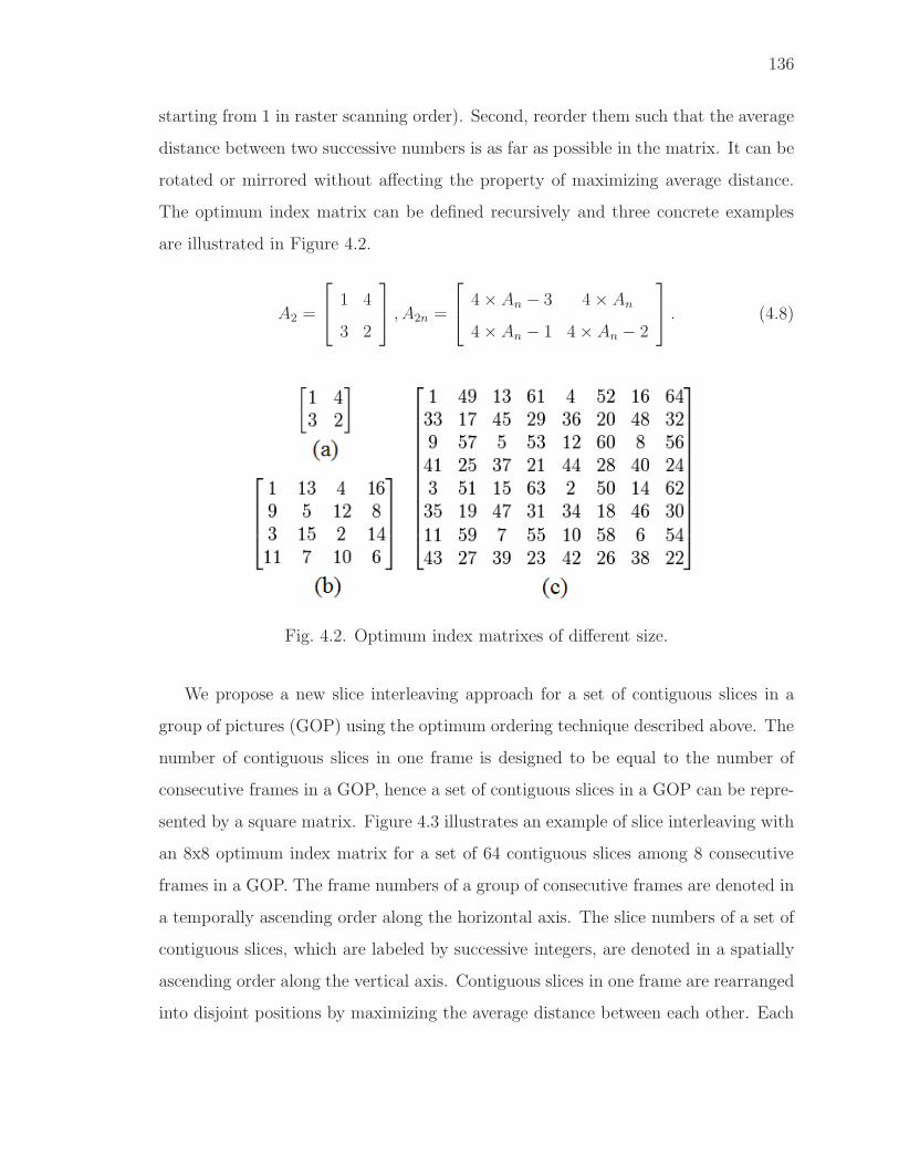
136
starting from 1 in raster scanning order). Second, reorder them such that the average
distance between two successive numbers is as far as possible in the matrix. It can be
rotated or mirrored without affecting the property of maximizing average distance.
The optimum index matrix can be defined recursively and three concrete examples
are illustrated in Figure 4.2.
A2 =
⎡⎣ 1 4
3 2
⎤⎦ , A2n =
⎡⎣ 4× An − 3 4× An
4× An − 1 4× An − 2
⎤⎦ . (4.8)
Fig. 4.2. Optimum index matrixes of different size.
We propose a new slice interleaving approach for a set of contiguous slices in a
group of pictures (GOP) using the optimum ordering technique described above. The
number of contiguous slices in one frame is designed to be equal to the number of
consecutive frames in a GOP, hence a set of contiguous slices in a GOP can be repre-
sented by a square matrix. Figure 4.3 illustrates an example of slice interleaving with
an 8x8 optimum index matrix for a set of 64 contiguous slices among 8 consecutive
frames in a GOP. The frame numbers of a group of consecutive frames are denoted in
a temporally ascending order along the horizontal axis. The slice numbers of a set of
contiguous slices, which are labeled by successive integers, are denoted in a spatially
ascending order along the vertical axis. Contiguous slices in one frame are rearranged
into disjoint positions by maximizing the average distance between each other. Each
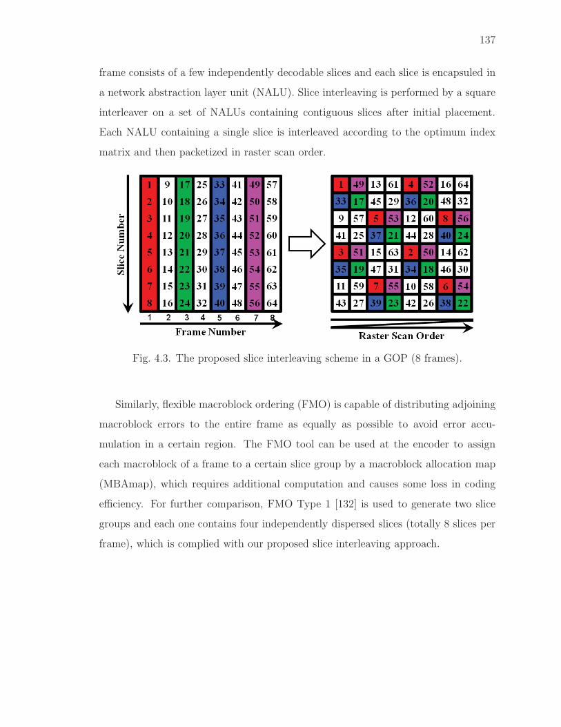
137
frame consists of a few independently decodable slices and each slice is encapsuled in
a network abstraction layer unit (NALU). Slice interleaving is performed by a square
interleaver on a set of NALUs containing contiguous slices after initial placement.
Each NALU containing a single slice is interleaved according to the optimum index
matrix and then packetized in raster scan order.
Fig. 4.3. The proposed slice interleaving scheme in a GOP (8 frames).
Similarly, flexible macroblock ordering (FMO) is capable of distributing adjoining
macroblock errors to the entire frame as equally as possible to avoid error accu-
mulation in a certain region. The FMO tool can be used at the encoder to assign
each macroblock of a frame to a certain slice group by a macroblock allocation map
(MBAmap), which requires additional computation and causes some loss in coding
efficiency. For further comparison, FMO Type 1 [132] is used to generate two slice
groups and each one contains four independently dispersed slices (totally 8 slices per
frame), which is complied with our proposed slice interleaving approach.

138
4.2 System Implementation
A two-layer spatial-temporal scalable video coding (SVC) system was developed
based on JSVM 9.8 [145], which was the last version officially supporting error con-
cealment tools. Sixty-four independently decodable slices in a GOP (8 frames in BL
and EL separately) are interleaved using the 8x8 optimum index matrix in Figure 4.3
at the encoder and correspondingly de-interleaved at the decoder. Each interleaved
slice was encapsulated into a single NALU during packetization. The parameters and
syntax elements of the 8x8 optimum index matrix and FMO Type 1 are independently
encoded into a picture parameter set (PPS) and transmitted to the decoder. The ex-
tra bits used for encoding these information were counted in the total bitrates. We
modified the JSVM reference decoder to deal with lost NALUs and conceal damaged
frames. It is able to manage the order of the NALUs received at decoder and iden-
tify the decoding information of the layer and slice in the received NALUs. Similar
to [146], a block-based status map is developed for each layer to inform the decoder
to decode available blocks and conceal lost blocks. The status map is reinitialized at
the beginning of decoding each slice.
Burst packet losses were simulated by removing NALUs from the encoded SVC
bitstreams based on random burst packet losses at different rates. Gilbert’s two-state
Markov model [147, 148] was used to independently generate random burst packet
loss patterns. This model can reasonably approximate Internet transmission [17].
In the good state G, all packets are correctly received, while in the bad state B,
all packets are lost. Two transition probabilities, pGB for going from G to B and
pBG for going from B to G, are sufficient to define the model. Moreover, other two
quantities are preferred to use: average burst packet loss probability PB = Pr(B) =
pGB/(pGB + pBG), the same as the well-defined burst packet loss rate (BPLR), and
average burst packet loss length LB = 1/pBG. The network simulation parameters
are defined using a pair (PB, LB). In our experiments, SVC video transmission over
burst packet loss channels are simulated in two scenarios: first corresponding to

139
(PB, LB) = (10%, 5) and second corresponding to (PB, LB) = (20%, 4). Damaged
frame are recovered by different error concealment methods, including three proposed
inter-layer methods using the two new approaches and FMO described above, i.e. (1)
motion vector averaging (MVAvg), (2) motion vector averaging and slice interleaving
(MVAvg+SliceIntlv) and (3) motion vector averaging, slice interleaving and FMO
(MVAvg+SliceIntlv+FMO), and two existing methods, i.e. (4) motion copy (MC) [18]
and (5) motion projection (MP) [142]. Because the original MC and MP methods
are developed for single-layer error concealment, the BLSkip-based extensions [18] of
the two methods are developed for inter-layer EC.
140
4.3 Experimental Results
Three video sequences with 300 frames, i.e. Bus, Football and Foreman, were used
to test our SVC system. The Bus sequence contains slow and homogenous motion
while the Football sequence has fast and chaotic motion. The Foreman sequence
involves normal motion and scene changes. Our experiments used the same quan-
tization parameter (QP) for encoding BL and EL frames (QP=28, 32, 36 and 40)
to evaluate different error concealment methods, running on a Linux desktop with a
2.8 GHz Quad-core CPU and 4 GB RAM. The frame coding structure was “IPP· · · ”with I-frame refresh after 2 successive P-frame GOPs in BL and 4 successive P-frame
GOPs in EL. For low complexity, we constantly set the parameter α = 0.5 and em-
ployed the 4-neighborhood of adjoining blocks s = 4. The average PSNR value of the
Y component (Y-PSNR) of damaged frames was used as an objective visual quality
measurement. The Y-PSNR was obtained by averaging the results of 50 random
burst packet loss patterns at each BPLR to ensure statistical significance of the re-
sults. Each burst packet loss pattern has 20 temporally circular shifts across the
entire frames, in total 20×50=1000 realizations of burst packet losses at a BPLR.
Table 4.1 demonstrates the average decoding time per frame of the existing and
proposed error concealment methods. The results show that the computational time
of the proposed MVAvg method is slightly longer than the MP and MC method.
It can be observed that the decoding delay (time difference between MVAvg-based
methods) caused by slice de-interleaving is relatively shorter than that introduced by
FMO.
The Y-PSNR of the first 60 frames of BL and EL Football sequence are illustrated
in Figure 4.4 and 4.5 with two concrete burst packet loss patterns at BPLR 10% and
20%, where the vertical dash lines indicate the damaged frames where burst packet
losses occurred. The visual quality in the enhancement layer is recovered slightly
faster than that in the base layer and the Y-PSNR drop in the enhancement layer
is comparatively smaller than that in the base layer. Visual distortion due to poorly

141
Table 4.1Average Decoding Time per Frame of the Existing and Proposed ErrorConcealment Methods (in Milliseconds)
Bus Football Foreman
Motion Copy (MC) 16.36 16.59 16.25
Motion Projection (MP) 17.33 17.82 17.14
MVAvg 17.94 18.53 17.68
MVAvg+SliceIntlv 19.95 20.60 19.72
MVAvg+SliceIntlv+FMO 24.08 24.76 23.87
concealed motion vectors is barely observed in the proposed three methods, except
for fast moving objects.

142
0 10 20 30 40 50 6014
16
18
20
22
24
26
28
30
32
Frame Number
Y−P
SN
R (d
B)
Football Base Layer (BPLR=10%)
Error FreeMVAvg+SliceIntlv+FMOMVAvgMVAvg+SliceIntlvMotion ProjectionMotion CopyCorrupted Frames
0 10 20 30 40 50 6014
16
18
20
22
24
26
28
30
32
Frame Number
Y−P
SN
R (d
B)
Football Enhancement Layer (BPLR=10%)
Error FreeMVAvg+SliceIntlv+FMOMVAvgMVAvg+SliceIntlvMotion ProjectionMotion CopyCorrupted Frames
Fig. 4.4. Y-PSNR of the Football BL & EL frames (BPLR=10%).

143
0 10 20 30 40 50 6014
16
18
20
22
24
26
28
30
32
Frame Number
Y−P
SN
R (d
B)
Football Base Layer (BPLR=20%)
Error FreeMVAvg+SliceIntlv+FMOMVAvgMVAvg+SliceIntlvMotion ProjectionMotion CopyCorrupted Frames
0 10 20 30 40 50 6014
16
18
20
22
24
26
28
30
32
Frame Number
Y−P
SN
R (d
B)
Football Enhancement Layer (BPLR=20%)
Error FreeMVAvg+SliceIntlv+FMOMVAvgMVAvg+SliceIntlvMotion ProjectionMotion CopyCorrupted Frames
Fig. 4.5. Y-PSNR of the Football BL & EL frames (BPLR=20%).

144
Compared with the perfect reconstruction from the error-free channel, the oper-
ational rate-distortion (RD) plots for various error concealment methods are shown
in Figure 4.6, 4.7 and 4.8. The proposed MVAvg method based on motion vec-
tor averaging is more effective than two existing methods in reducing the visual
quality degradation caused by burst packet losses and error propagation. The RD
plots illustrate that the Y-PSNR of the proposed MVAvg method is 0.9dB-3.2dB
higher than the existing MC method and is 0.3dB-2.1dB higher than the existing MP
method. The proposed MVAvg+SliceIntlv+FMO and MVAvg+SliceIntlv methods
outperform the other methods in significantly improving the visual quality. In fact,
the RD plots of the two methods are very close at low bitrate and low BPLR. The
MVAvg+SliceIntlv+FMO method is superior to the MVAvg+SliceIntlv method only
at high bitrate and high BPLR, because additional bit overhead for encoding FMO in-
formation undermines the coding efficiency at low bitrate. Therefore, considering the
tradeoff between complexity and performance, The the proposed MVAvg+SliceIntlv
method is more suitable for low burst packet loss channel.

145
Fig. 4.6. Rate-Distortion of the Bus sequence (BPLR=10%, 20%).
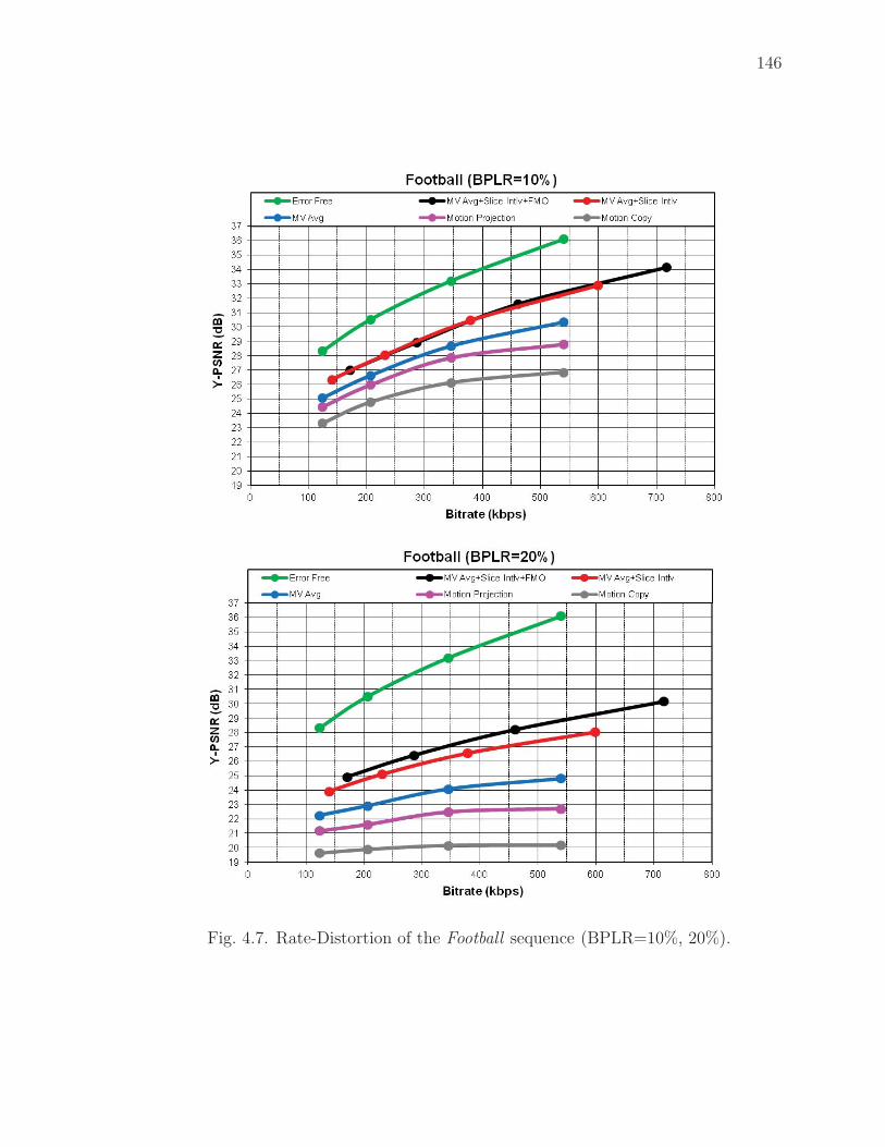
146
Fig. 4.7. Rate-Distortion of the Football sequence (BPLR=10%, 20%).

147
Fig. 4.8. Rate-Distortion of the Foreman sequence (BPLR=10%, 20%).

148
5. CONCLUSIONS AND FUTURE WORK
5.1 Conclusions
In this thesis we describe several visual saliency models in the frequency domain in
Chapter 2, a hazmat sign image analysis system (MERGE) using visual saliency for
location detection and content recognition in Chapter 3, and several error concealment
methods for scalable video coding (SVC) in chapter 4.
For visual saliency models in the frequency domain, we develop separate and
composite visual saliency model families for frequency domain visual saliency models.
We propose six visual saliency models based on new spectrum processing methods
and an entropy-based saliency map selection approach. We propose an entropy-
based saliency map selection approach to select a “good” final saliency map among
the set of map candidates. A group of extended saliency models that extends each
proposed visual saliency models are also developed by incorporating both separate
and composite model families and using variant color spaces. Experimental results
show that the six best extended models are more accurate and efficient than most
state-of-the-art models in predicting eye fixation on standard image datasets.
For hazmat sign image analysis system (MERGE), we develop hazmat sign lo-
cation detection and content recognition methods based on visual saliency. We use
the one of our proposed frequency domain models to extract salient regions that are
likely to contain hazmat sign candidates and then use a Fourier descriptor based con-
tour matching method to locate the border of hazmat signs in these regions. This
visual saliency based approach is able to increase the accuracy of sign location de-
tection, significantly reduce the number of false positives, and speed up the image
analysis process. This approach improves the accuracy of existing methods presented
in [14, 15]. We also propose a color recognition method to interpret the color inside
149
the detected hazmat signs. Our three image datasets consists of images taken in
the working field and outdoor field under variant lighting and weather conditions,
distances, and perspectives.
For error concealment for scalable video coding (SVC), we develop two error con-
cealment approaches robust to burst packet losses, i.e. inter-layer motion vector av-
eraging and slice interleaving using optimum ordering. A two-layer spatial-temporal
scalable video coding system are decribed to evaluate the existing and proposed error
concealment methods. Experimental results confirmed that the proposed error con-
cealment methods outperform two existing methods in reducing the impact of burst
packet losses and error propagation.
The main contributions of visual saliency models in the frequency domain are:
• We investigate bottom-up visual saliency using spectral analysis approaches.
• We develop separate and composite visual saliency model families for frequency
domain models.
• We propose six visual saliency models based on different spectrum processing.
• We propose an entropy-based saliency map selection approach.
• We develop an evaluation tool for benchmarking visual saliency models.
The main contributions of image analysis system for hazmat sign detection and
recognition are:
• We develop a hazmat sign location detection and content recognition system
using visual saliency.
• We used one of our proposed frequency domain models to extract salient regions.
• We developed a Fourier descriptor based contour matching method to locate
the border of hazmat signs.

150
• We proposed a color recognition method to interpret the color inside the de-
tected hazmat signs.
• We collected three hazmat sign image datasets.
The main contributions of error concealment methods for SVC are:
• We investigated the impact of burst packet loss and error propagation in base
and enhancement layers.
• We explored inter-layer spatial and temporal correlations for error concealment
against burst packet loss.
• We proposed two error concealment methods to enhance error recovery and
visual quality:
• (1) Inter-layer motion vector averaging
• (2) Slice interleaving using optimum ordering
• We developed a two-layer spatial-temporal scalable video coding system for
evaluation.
5.2 Future Work
Our long term goal for MERGE is to develop a hazmat sign image analysis sys-
tem capable of automatically recognizing hazmat signs from images acquired up to
300 feet and providing real-time guide information to first responders to identify the
hazardous materials and determine what specialty equipment, procedures and pre-
cautions should be taken in the event of an emergency.
One problem is the overall accuracy of our hazmat sign image analysis methods.
The accuracy needs to be improved. This can be done by improving our current sign
location detection approach and developing more robust color recognition techniques.
We may be able to use supper-resolution image reconstruction methods [126, 127] to
151
refine the hazmat sign images. It can improve the location detection accuracy at even
longer distances and it is more useful for blurred and low resolution hazmat signs.
We can also employ proper color calibration [51]. This can help the color recognition
technique to recognize colored hazmat signs more accurately. One could also use
character recognition methods to interpret the text inside the detected hazmat signs
when the image resolution is relatively high.
For visual saliency models in the frequency domain, one direction of future work
is testing our proposed visual saliency models using more eye fixation image datasets.
One could also study the tradeoff between accuracy and speed of the proposed fre-
quency domain saliency models for practical applications. Another direction is com-
bining several saliency models to achieve better accuracy of predicting eye fixation
and hazmat sign image analysis.
For error concealment for scalable video coding (SVC), one direction of future work
is testing our proposed error concealment models on high resolution video sequences.
5.3 Publications Resulting from This Work
Conference Papers
1. Bin Zhao and Edward J. Delp, “Visual Saliency Models Based on Spectrum
Processing,” Proceedings of the IEEE Winter Conference on Applications of
Computer Vision, Waikoloa Beach, HI, USA, January 2015. (Accepted)
2. Bin Zhao, Albert Parra, and Edward J. Delp, “Mobile-Based Hazmat Sign
Detection and Recognition,” Proceedings of the IEEE Global Conference on
Signal and Information Processing, no. 6736996, pp. 735-738, Austin, TX,
USA, December 2013. (Invited Paper)
3. Bin Zhao and Edward J. Delp, “Inter-layer Error Concealment for Scalable
Video Coding,” Proceedings of the IEEE International Conference on Multime-
dia and Expo, no. 6607539, pp. 1-6, San Jose, CA, USA, July 2013.
152
4. Bin Zhao, “Interleaving-Based Error Concealment for Scalable Video Coding
System,” Proceedings of the IEEE Visual Communications and Image Process-
ing Conference, no. 6115965, pp. 1-4, Tainan City, Taiwan, November 2011.
5. Albert Parra, Bin Zhao, Joonsoo Kim, and Edward J. Delp, “Recognition,
Segmentation and Retrieval of Gang Graffiti Images on a Mobile Device,” Pro-
ceedings of the IEEE International Conference on Technologies for Homeland
Security, no. 6698996, pp. 178-183, Waltham, MA, USA, November 2013.
6. Albert Parra, Bin Zhao, Andrew Haddad, Mireille Boutin, and Edward J.
Delp, “Hazardous Material Sign Detection and Recognition,” Proceedings of the
IEEE International Conference on Image Processing, no. 6738544, pp. 2640-
2644, Melbourne, Australia, September 2013.
Journal Papers
1. Bin Zhao and Edward J. Delp, “Biologically-Inspired Visual Saliency Models
Using Spectrum Processing,” in preparation.
2. Bin Zhao, Albert Parra, and Edward J. Delp, “Hazmat Sign Detection and
Recognition Using Visual Saliency,” in preparation.

LIST OF REFERENCES

153
LIST OF REFERENCES
[1] ERG, available: http://www.phmsa.dot.gov/hazmat/library/erg.
[2] L. Itti, “Models of bottom-up and top-down visual attention,” Ph.D. disserta-tion, California Institute of Technology, 2000.
[3] C. Koch and S. Ullman, “Shifts in selective visual attention: Towards theunderlying neural circuitry,” Human Neurobiology, vol. 4, no. 4, pp. 219–227,April 1985.
[4] A. M. Treisman and G. Gelade, “A feature-integration theory of attention,”Cognitive Psychology, vol. 12, no. 1, pp. 97–136, January 1980.
[5] J. M. Wolfe, “Guided search 2.0 A revised model of visual search,” PsychonomicBulletin & Review, vol. 1, no. 2, pp. 202–238, 1994.
[6] J. M. Wolfe and T. S. Horowitz, “What attributes guide the deployment ofvisual attention and how do they do it?” Nature Reviews Neuroscience, vol. 5,no. 6, pp. 495–501, June 2004.
[7] S. Frintrop, E. Rome, and H. I. Christensen, “Computational visual attentionsystems and their cognitive foundations: A survey,” ACM Transactions onApplied Perception, vol. 7, no. 1, pp. 6:1–6:39, January 2010.
[8] A. Toet, “Computational versus psychophysical bottom-up image saliency: Acomparative evaluation study,” IEEE Transactions on Pattern Analysis andMachine Intelligence, vol. 33, no. 11, pp. 2131–2146, November 2011.
[9] A. Borji and L. Itti, “State-of-the-art in visual attention modeling,” IEEETransactions on Pattern Analysis and Machine Intelligence, vol. 35, no. 1, pp.185–207, January 2013.
[10] A. Borji, D. N. Sihite, and L. Itti, “Quantitative analysis of human-model agree-ment in visual saliency modeling: A comparative study,” IEEE Transactionson Image Processing, vol. 22, no. 1, pp. 55–69, January 2013.
[11] United States Department of Transportation, Code of Federal Regulations,Title 49 - Transportation, 2012nd ed., October 2012.
[12] WISER, available: http://wiser.nlm.nih.gov.
[13] MERGE, available: http://www.hazmat-signs.org.
[14] B. Zhao, A. Parra, and E. J. Delp, “Mobile-based hazmat sign detectionsystem,” Proceedings of the IEEE Global Conference on Signal and InformationProcessing, pp. 735–738, December 2013, Austin, TX, USA.
154
[15] A. Parra, B. Zhao, A. Haddad, M. Boutin, and E. J. Delp, “Hazardousmaterial sign detection and recognition,” Proceedings of the IEEE InternationalConference on Image Processing, pp. 2640–2644, September 2013, Melbourne,Australia.
[16] H. Schwarz, D. Marpe, and T. Wiegand, “Overview of the scalable video codingextension of the H.264/AVC standard,” IEEE Transactions on Circuits andSystems for Video Technology, vol. 17, no. 9, pp. 1103–1120, September 2007.
[17] K. Stuhlmuller, N. Farber, M. Link, and B. Girod, “Analysis of video transmis-sion over lossy channels,” IEEE Journal on Selected Areas in Communications,vol. 18, no. 6, pp. 1012–1032, June 2000.
[18] Y. Guo, Y. Chen, Y.-K. Wang, H. Li, M. M. Hannuksela, and M. Gabbouj,“Error resilient coding and error concealment in scalable video coding,” IEEETransactions on Circuits and Systems for Video Technology, vol. 19, no. 6, pp.781–795, June 2009.
[19] C. Christopoulos, A. Skodras, and T. Ebrahimi, “The JPEG2000 still imagecoding system: An overview,” IEEE Transactions on Consumer Electronics,vol. 46, no. 4, pp. 1103–1127, November 2000.
[20] L. Itti, “Automatic foveation for video compression using a neurobiologicalmodel of visual attention,” IEEE Transactions on Image Processing, vol. 13,no. 10, pp. 1304–1318, October 2004.
[21] S. Avidan and A. Shamir, “Seam carving for content-aware image resizing,”ACM Transactions on Graphics, vol. 26, no. 3, pp. 1–9, July 2007.
[22] J. Han, K. N. Ngan, M. Li, and H. Zhang, “Unsupervised extraction of visualattention objects in color images,” IEEE Transactions on Circuits and Systemsfor Video Technology, vol. 16, no. 1, pp. 141–145, January 2006.
[23] D. Walther and C. Koch, “Modeling attention to salient proto-objects,” NeuralNetworks, vol. 19, no. 9, pp. 1395–1407, November 2006.
[24] A. Mogelmose, M. M. Trivedi, and T. B. Moeslund, “Vision-based traffic signdetection and analysis for intelligent driver assistance systems: Perspectivesand survey,” IEEE Transactions on Intelligent Transportation Systems, vol. 13,no. 4, pp. 1484–1497, December 2012.
[25] L. Itti, C. Koch, and E. Niebur, “A model of saliency-based visual attentionfor rapid scene analysis,” IEEE Transactions on Pattern Analysis and MachineIntelligence, vol. 20, no. 11, pp. 1254–1259, November 1998.
[26] J. Harel, C. Koch, and P. Perona, “Graph-based visual saliency,” Proceedingsof the Annual Conference on Neural Information Processing Systems, pp.545–552, December 2006, Vancouver, BC, Canada.
[27] N. D. B. Bruce and J. K. Tsotsos, “Saliency, attention, and visual search: Aninformation theoretic approach,” Journal of Vision, vol. 9, no. 3, pp. 1–24,March 2009.
[28] X. Hou and L. Zhang, “Dynamic visual attention: Searching for coding lengthincrements,” Proceedings of the Annual Conference on Neural InformationProcessing Systems, pp. 681–688, December 2008, Vancouver, BC, Canada.

155
[29] R. Achanta, S. Hemami, F. Estrada, and S. Susstrunk, “Frequency-tuned salientregion detection,” Proceedings of the IEEE Conference on Computer Vision andPattern Recognition, pp. 1597–1604, June 2009, Miami, FL, USA.
[30] C. Guo, Q. Ma, and L. Zhang, “Spatio-temporal saliency detection using phasespectrum of quaternion Fourier transform,” Proceedings of the IEEE Conferenceon Computer Vision and Pattern Recognition, pp. 1–8, June 2008, Anchorage,AK, USA.
[31] C. Guo and L. Zhang, “A novel multiresolution spatiotemporal saliency de-tection model and its applications in image and video compression,” IEEETransactions on Image Processing, vol. 19, no. 1, pp. 185–198, January 2010.
[32] P. Bian and L. Zhang, “Visual saliency: A biologically plausible contourlet-likefrequency domain approach,” Cognitive Neurodynamics, vol. 4, no. 3, pp.189–198, September 2010.
[33] X. Hou, J. Harel, and C. Koch, “Image signature: Highlighting sparse salientregions,” IEEE Transactions on Pattern Analysis and Machine Intelligence,vol. 34, no. 1, pp. 194–201, January 2012.
[34] B. Schauerte and R. Stiefelhagen, “Predicting human gaze using quaternionDCT image signature saliency and face detection,” Proceedings of the IEEEWorkshop on Applications of Computer Vision, pp. 137–144, January 2012,Breckenridge, CO, USA.
[35] J. Li, M. D. Levine, X. An, X. Xu, and H. He, “Visual saliency based onscale-space analysis in the frequency domain,” IEEE Transactions on PatternAnalysis and Machine Intelligence, vol. 35, no. 4, pp. 996–1010, April 2013.
[36] T. A. Ell, “Quaternion-Fourier transforms for analysis of two-dimensional lineartime-invariant partial differential systems,” Proceedings of the IEEE Conferenceon Decision and Control, vol. 2, pp. 1830–1841, December 1993, San Antonio,TX, USA.
[37] T. A. Ell and S. J. Sangwine, “Hypercomplex Fourier transforms of color im-ages,” IEEE Transactions on Image Processing, vol. 16, no. 1, pp. 22–35, Jan-uary 2007.
[38] L. Zhang, M. H. Tong, T. K. Marks, H. Shan, and G. W. Cottrell, “SUN: Abayesian framework for saliency using natural statistics,” Journal of Vision,vol. 8, no. 7, pp. 1–20, December 2008.
[39] Y. Fang, W. Lin, B.-S. Lee, C.-T. Lau, Z. Chen, and C.-W. Lin, “Bottom-up saliency detection model based on human visual sensitivity and amplitudespectrum,” IEEE Transactions on Multimedia, vol. 14, no. 1, pp. 187–198,February 2012.
[40] Z. Li, “A saliency map in primary visual cortex,” Trends in Cognitive Sciences,vol. 6, no. 1, pp. 9–16, January 2002.
[41] Z. Li and P. Dayan, “Pre-attentive visual selection,” Neural Networks, vol. 19,no. 9, pp. 1437–1439, November 2006.
156
[42] C. A. Curcio, K. R. Sloan, R. E. Kalina, and A. E. Hendrickson, “Humanphotoreceptor topography,” The Journal of Comparative Neurology, vol. 292,no. 4, pp. 497–523, February 1990.
[43] E. D. Montag, Rods and Cones, available:http://www.cis.rit.edu/people/faculty/montag/vandplite/pages/chap 9/ch9p1.html.
[44] C. Blakemore and F. W. Campbell, “On the existence of neurones in thehuman visual system selectively sensitive to the orientation and size of retinalimages,” The Journal of Physiology, vol. 203, no. 1, pp. 237–260, July 1969.
[45] D. Casasent and D. Psaltis, “New optical transforms for pattern recognition,”Proceedings of the IEEE, vol. 65, no. 1, pp. 77–84, January 1977.
[46] P. Cavanagh, “Size and position invariance in the visual system,” Perception,vol. 7, no. 2, pp. 167–177, 1978.
[47] ——, “Size invariance: Reply to Schwartz,” Perception, vol. 10, no. 4, pp.469–474, 1981.
[48] L. O. Harvey and V. V. Doan, “Visual masking at different polar angles in thetwo-dimensional Fourier plane,” Journal of the Optical Society of America A,vol. 7, no. 1, pp. 116–127, January 1990.
[49] E. L. Schwartz, “Spatial mapping in the primate sensory projection: Analyticstructure and relevance to perception,” Biological Cybernetics, vol. 25, no. 4,pp. 181–194, 1977.
[50] ——, “Computational anatomy and functional architecture of striate cortex:A spatial mapping approach to perceptual coding,” Vision Research, vol. 20,no. 8, pp. 645–669, 1980.
[51] H.-C. Lee, Color Imaging Science. Cambridge, UK: Cambridge UniversityPress, 2005.
[52] M. D. Fairchild, Color Appearance Models. Chichester, UK: Wiley-IS&T, 2013.
[53] S. Susstrunk, R. Buckley, and S. Swen, “Standard RGB color spaces,” Proceed-ings of the Color Imaging Conference: Color Science, Systems, and Applica-tions, pp. 127–134, November 1999, Scottsdale, AZ, USA.
[54] S. Engel, X. Zhang, and B. Wandell, “Colour tuning in human visual cortexmeasured with functional magnetic resonance imaging,” Nature, vol. 388, no.6637, pp. 68–71, July 1997.
[55] W. R. Hamilton, Elements of Quaternions. Dublin, Ireland: The Universityof Dublin Press, 1866.
[56] P. Bian and L. Zhang, “Biological plausibility of spectral domain approach forspatiotemporal visual saliency,” Proceedings of the International ConferenceNeuro-Information Processing, vol. 5506, pp. 251–258, November 2008,Auckland, New Zealand.
[57] B. Schauerte and R. Stiefelhagen, “Quaternion-based spectral saliencydetection for eye fixation prediction,” Proceedings of the European Conferenceon Computer Vision, pp. 116–129, October 2012, Florence, Italy.
157
[58] W. Feng and B. Hu, “Quaternion discrete cosine transform and its application incolor template matching,” Proceedings of the International Congress on Imageand Signal Processing, vol. 2, pp. 252–256, May 2008, Sanya, China.
[59] K. Castleman, Digital Image Processing. New York, USA: Prentice-Hall, 1996.
[60] A. V. Oppenheim and J. S. Lim, “The importance of phase in signals,” Pro-ceedings of the IEEE, vol. 69, no. 5, pp. 529–541, May 1981.
[61] M. H. Hayes, J. S. Lim, and A. V. Oppenheim, “Signal reconstruction fromphase or magnitude,” IEEE Transactions on Acoustics, Speech and Signal Pro-cessing, vol. 28, no. 6, pp. 672–680, December 1980.
[62] J. W. Cooley and J. W. Tukey, “An algorithm for the machine calculationof complex Fourier series,” Mathematics of Computation, vol. 19, no. 90, pp.297–301, April 1965.
[63] B. A. Olshausen and D. J. Field, “Emergence of simple-cell receptive fieldproperties by learning a sparse code for natural images,” Nature, vol. 381, no.6583, pp. 607–609, June 1996.
[64] D. J. Graham and D. J. Field, “Natural images: Coding efficiency,”Encyclopedia of Neuroscience, pp. 19–27, 2009.
[65] X. Hou and L. Zhang, “Saliency detection: A spectral residual approach,” Pro-ceedings of the IEEE Conference on Computer Vision and Pattern Recognition,pp. 1–8, June 2007, Minneapolis, MN, USA.
[66] C. A. Poynton, “Rehabilitation of gamma,” Proceedings of the SPIE Conferenceon Human Vision and Electronic Imaging III, vol. 3299, pp. 232–249, January1998, San Jose, CA, USA.
[67] S. S. Stevens, “On the psychophysical law,” Psychological Review, vol. 64,no. 3, pp. 153–181, May 1957.
[68] R. J. Peters, A. Iyer, L. Itti, and C. Koch, “Components of bottom-up gazeallocation in natural images,” Vision Research, vol. 45, no. 18, pp. 2397–2416,August 2005.
[69] S. Kullback, Information Theory and Statistics. New York, USA: Wiley, 1959.
[70] L. Itti and P. Baldi, “A principled approach to detecting surprising events invideo,” Proceedings of the IEEE Conference on Computer Vision and PatternRecognition, vol. 1, pp. 631–637, June 2005, San Diego, CA, USA.
[71] T. Jost, N. Ouerhani, R. von Wartburg, R. Mri, and H. Hgli, “Assessingthe contribution of color in visual attention,” Computer Vision and ImageUnderstanding, vol. 100, no. 1-2, pp. 107–123, Oct.-Nov. 2005.
[72] D. M. Green and J. A. Swets, Signal Detection Theory and Psychophysics. NewYork, USA: Wiley, 1966.
[73] B. W. Tatler, R. J. Baddeley, and I. D. Gilchrist, “Visual correlates of fixationselection: Effects of scale and time,” Vision Research, vol. 45, no. 5, pp.643–659, March 2005.

158
[74] F. Larsson, M. Felsberg, and P.-E. Forssen, “Correlating fourier descriptors oflocal patches for road sign recognition,” IET Computer Vision, vol. 5, no. 4,pp. 244–254, July 2011.
[75] T. Gevers and A. W. M. Smeulders, “Color-based object recognition,” PatternRecognition, vol. 32, no. 3, pp. 453–464, March 1999.
[76] C. Grigorescu and N. Petkov, “Distance sets for shape filters and shape recogni-tion,” IEEE Transactions on Image Processing, vol. 12, no. 10, pp. 1274–1286,October 2003.
[77] D. Gossow, J. Pellenz, and D. Paulus, “Danger sign detection using color his-tograms and SURF matching,” Proceedings of the IEEE International Work-shop on Safety, Security and Rescue Robotics, pp. 13–18, October 2008, Sendai,Japan.
[78] A. Broggi, P. Cerri, P. Medici, P. Porta, and G. Ghisio, “Real time road signsrecognition,” Proceedings of the IEEE Intelligent Vehicles Symposium, pp. 981–986, June 2007, Istambul, Turkey.
[79] K. L. Bouman, G. Abdollahian, M. Boutin, and E. J. Delp, “A low complexitysign detection and text localization method for mobile applications,” IEEETransactions on Multimedia, vol. 13, no. 5, pp. 922–934, October 2011.
[80] L. Song and Z. Liu, “Color-based traffic sign detection,” Proceedings of theInternational Conference on Quality, Reliability, Risk, Maintenance, and SafetyEngineering, pp. 353–357, June 2012, Chengdu, China.
[81] G. Loy and N. Barnes, “Fast shape-based road sign detection for a driver as-sistance system,” Proceedings of the IEEE/RSJ International Conference onIntelligent Robots and Systems, vol. 1, pp. 70–75, September 2004, Stockholm,Sweden.
[82] S. Maldonado-Bascon, S. Lafuente-Arroyo, P. Gil-Jimenez, H. Gomez-Moreno,and F. Lopez-Ferreras, “Road-sign detection and recognition based on supportvector machines,” IEEE Transactions on Intelligent Transportation Systems,vol. 8, no. 2, pp. 264–278, June 2007.
[83] R. Malik, J. Khurshid, and S. N. Ahmad, “Road sign detection and recognitionusing colour segmentation, shape analysis and template matching,” Proceedingsof the International Conference on Machine Learning and Cybernetics, vol. 6,pp. 3556–3560, August 2007, Hong Kong, China.
[84] J. Greenhalgh and M. Mirmehdi, “Real-time detection and recognition of roadtraffic signs,” IEEE Transactions on Intelligent Transportation Systems, vol. 13,no. 4, pp. 1498–1506, December 2012.
[85] W.-J. Won, M. Lee, and J.-W. Son, “Implementation of road traffic signs detec-tion based on saliency map model,” Proceedings of the IEEE Intelligent VehiclesSymposium, pp. 542–547, June 2008, Eindhoven, Netherlands.
[86] R. Kastner, T. Michalke, T. Burbach, J. Fritsch, and C. Goerick, “Attention-based traffic sign recognition with an array of weak classifiers,” Proceedings ofthe IEEE Intelligent Vehicles Symposium, pp. 333–339, June 2010, San Diego,CA, USA.

159
[87] R. Belaroussi, P. Foucher, J.-P. Tarel, B. Soheilian, P. Charbonnier, and N. Pa-paroditis, “Road sign detection in images: A case study,” Proceedings of theInternational Conference on Pattern Recognition, pp. 484–488, August 2010,Istambul, Turkey.
[88] D. C. W. Pao, H. F. Li, and R. Jayakumar, “Shapes recognition using thestraight line Hough transform: Theory and generalization,” IEEE Transactionson Pattern Analysis and Machine Intelligence, vol. 14, no. 11, pp. 1076–1089,November 1992.
[89] S. Houben, “A single target voting scheme for traffic sign detection,” Proceedingsof the IEEE Intelligent Vehicles Symposium, pp. 124–129, June 2011, Baden-Baden, Germany.
[90] H. Fleyeh and P. Zhao, “A contour-based separation of vertically attached trafficsigns,” Proceedings of the Annual Conference of the IEEE Industrial ElectronicsSociety, pp. 1811–1816, November 2008, Orlando, FL, USA.
[91] L.-W. Tsai, J.-W. Hsieh, C.-H. Chuang, Y.-J. Tseng, K.-C. Fan, and C.-C. Lee,“Road sign detection using eigen colour,” IET Computer Vision, vol. 2, no. 3,pp. 164–177, September 2008.
[92] G. Loy and A. Zelinsky, “Fast radial symmetry for detecting points of interest,”IEEE Transactions on Pattern Analysis and Machine Intelligence, vol. 25, no. 8,pp. 959–973, August 2003.
[93] N. Barnes, A. Zelinsky, and L. Fletcher, “Real-time speed sign detection usingthe radial symmetry detector,” IEEE Transactions on Intelligent Transporta-tion Systems, vol. 9, no. 2, pp. 322–332, June 2008.
[94] P. Viola and M. J. Jones, “Robust real-time face detection,” InternationalJournal of Computer Vision, vol. 57, no. 2, pp. 137–154, May 2004.
[95] C. G. Keller, C. Sprunk, C. Bahlmann, J. Giebel, and G. Baratoff, “Real-timerecognition of U.S. speed signs,” Proceedings of the IEEE Intelligent VehiclesSymposium, pp. 518–523, June 2008, Eindhoven, Netherlands.
[96] X. Baro, S. Escalera, J. Vitria, O. Pujol, and P. Radeva, “Traffic sign recognitionusing evolutionary Adaboost detection and Forest-ECOC classification,” IEEETransactions on Intelligent Transportation Systems, vol. 10, no. 1, pp. 113–126,March 2009.
[97] A. R. Rostampour and P. R. Madhvapathy, “Shape recognition using simplemeasures of projections,” Proceedings of the Annual International Phoenix Con-ference on Computers and Communications, pp. 474–479, March 1988, Scotts-dale, AZ, USA.
[98] P. Gil-Jimenez, S. Lafuente-Arroyo, H. Gomez-Moreno, F. Lopez-Ferreras, andS. Maldonado-Bascon, “Traffic sign shape classification evaluation. Part II. FFTapplied to the signature of blobs,” Proceedings of the IEEE Intelligent VehiclesSymposium, pp. 607–612, June 2005, Las Vegas, NV, USA.
[99] A. W. Haddad, S. Huang, M. Boutin, and E. J. Delp, “Detection of symmetricshapes on a mobile device with applications to automatic sign interpretation,”Proceedings of the IS&T/SPIE Electronic Imaging - Multimedia on Mobile De-vices, no. 8304, pp. 1–8, January 2012, San Francisco, CA, USA.
160
[100] T. Pavlidis, “A review of algorithms for shape analysis,” Computer Graphicsand Image Processing, vol. 7, no. 2, pp. 243–258, April 1978.
[101] ——, “Algorithms for shape analysis of contours and waveforms,” IEEE Trans-actions on Pattern Analysis and Machine Intelligence, vol. PAMI-2, no. 4, pp.301–312, July 1980.
[102] S. Belongie, J. Malik, and J. Puzicha, “Shape matching and object recognitionusing shape contexts,” IEEE Transactions on Pattern Analysis and MachineIntelligence, vol. 24, no. 4, pp. 509–522, April 2002.
[103] O. R. Mitchell and T. A. Grogan, “Global and partial shape discrimination forcomputer vision,” Optical Engineering, vol. 23, no. 5, pp. 484–491, October1984.
[104] C. T. Zahn and R. Z. Roskies, “Fourier descriptors for plane closed curves,”IEEE Transactions on Computers, vol. C-21, no. 3, pp. 269–281, March 1972.
[105] E. Persoon and K.-S. Fu, “Shape discrimination using Fourier descriptors,”IEEE Transactions on Systems, Man and Cybernetics, vol. SMC-7, no. 3, pp.170–179, March 1977.
[106] D. Zhang and G. Lu, “Evaluation of MPEG-7 shape descriptors against othershape descriptors,” Multimedia Systems, vol. 9, no. 1, pp. 15–30, July 2003.
[107] R. Chellappa and R. Bagdazian, “Fourier coding of image boundaries,” IEEETransactions onPattern Analysis and Machine Intelligence, vol. PAMI-6, no. 1,pp. 102–105, January 1984.
[108] C. Singh and P. Sharma, “Performance analysis of various local and globalshape descriptors for image retrieval,” Multimedia Systems, vol. 19, no. 4, pp.339–357, July 2013.
[109] I. Kunttu, L. Lepisto, J. Rauhamaa, and A. Visa, “Multiscale Fourier descriptorfor shape-based image retrieval,” Proceedings of the IEEE International Con-ference on Pattern Recognition, vol. 2, pp. 765–768, August 2004, Cambridge,UK.
[110] M. N. Tahir, A. Hussain, and M. M. Mustafa, “Fourier descriptor for pedestrianshape recognition using support vector machine,” Proceedings of the IEEE In-ternational Symposium on Signal Processing and Information Technology, pp.636–641, December 2007, Cairo, Egypt.
[111] J. Ma, Z. Zhang, H. Tang, and Q. Zhao, “Fast Fourier descriptor method of theshape feature in low resolution images,” Proceedings of the IEEE InternationalConference on Wireless Communications Networking and Mobile Computing,pp. 1–4, September 2010, Chengdu, China.
[112] J. Meyer, P. Schnitzspan, S. Kohlbrecher, K. Petersen, M. Andriluka,O. Schwahn, U. Klingauf, S. Roth, B. Schiele, and O. Stryk, “A semanticworld model for urban search and rescue based on heterogeneous sensors,”Proceedings of the Annual RoboCup International Symposium, vol. 6556, pp.180–193, June 2010, Singapore, Singapore.

161
[113] H. Bay, A. Ess, T. Tuytelaars, and L. V. Gool, “Speeded-up robust features(SURF),” Journal of Computer Vision and Image Understanding, vol. 110,no. 3, pp. 346–359, June 2008.
[114] N. Dalal and B. Triggs, “Histograms of oriented gradients for human detec-tion,” Proceedings of the IEEE Conference on Computer Vision and PatternRecognition, vol. 1, pp. 886–893, June 2005, San Diego, CA, USA.
[115] S. Suzuki and K. Abe, “Topological structural analysis of digitized binaryimages by border following,” Computer Vision, Graphics, and ImageProcessing, vol. 30, no. 1, pp. 32–46, April 1985.
[116] R. O. Duda and P. E. Hart, “Use of the Hough transformation to detect linesand curves in pictures,” Communications of the ACM, vol. 15, no. 1, pp.11–15, January 1972.
[117] J. Sklansky, “Finding the convex hull of a simple polygon,” Pattern RecognitionLetters, vol. 1, no. 2, pp. 79–83, December 1982.
[118] S. Pereira and T. Pun, “Robust template matching for affine resistant imagewatermarks,” IEEE Transactions on Image Processing, vol. 9, no. 6, pp. 1123–1129, Jun. 2000.
[119] F. Essannouni and D. Aboutajdine, “Fast frequency template matching usinghigher order statistics,” IEEE Transactions on Image Processing, vol. 19, no. 3,pp. 826–830, March 2010.
[120] I. Bartolini, P. Ciaccia, and M. Patella, “WARP: Accurate retrieval of shapesusing phase of Fourier descriptors and time warping distance,” IEEE Transac-tions on Pattern Analysis and Machine Intelligence, vol. 27, no. 1, pp. 142–147,January 2005.
[121] N. Otsu, “A threshold selection method from gray-level histograms,” IEEETransactions on Systems, Man and Cybernetics, vol. SMC-9, no. 1, pp. 62–66,January 1979.
[122] L.-S. Jin, L. Tian, R.-B. Wang, L. Guo, and J.-W. Chu, “An improved Otsuimage segmentation algorithm for path mark detection under variable illumi-nation,” Proceedings of the IEEE Intelligent Vehicles Symposium, pp. 840–844,June 2005, Las Vegas, NV, USA.
[123] P. Soille, Morphological Image Analysis: Principles and Applications. NewYork/Heidelberg: Springer-Verlag, 2003.
[124] H. Park and R. Chin, “Decomposition of arbitrarily shaped morphological struc-turing elements,” IEEE Transactions on Pattern Analysis and Machine Intel-ligence, vol. 17, no. 1, pp. 2–15, January 1995.
[125] R. C. Gonzalez, Digital Image Processing. New Jersey, USA: Prentice Hall,2000.
[126] S. C. Park, M. K. Park, and M. G. Kang, “Super-resolution image reconstruc-tion: A technical overview,” IEEE Signal Processing Magazine, vol. 20, no. 3,pp. 21–36, May 2003.

162
[127] W.-C. Siu and K.-W. Hung, “Review of image interpolation and super-resolution,” Proceedings of the Asia-Pacific Signal Information Processing As-sociation Annual Summit and Conference, no. 6411957, pp. 1–10, December2012, hollywood, CA, USA.
[128] Y. J. Liang, J. G. Apostolopoulos, and B. Girod, “Analysis of packet loss forcompressed video: Effect of burst losses and correlation between error frames,”IEEE Transactions on Circuits and Systems for Video Technology, vol. 18, no. 7,pp. 861–874, July 2008.
[129] Y. Wang and Q.-F. Zhu, “Error control and concealment for video communi-cation: A review,” Proceedings of the IEEE, vol. 86, no. 5, pp. 974–997, May1998.
[130] S. Kumar, L. Xu, M. K. Mandal, and S. Panchanathan, “Error resiliencyschemes in H.264/AVC standard,” Journal of Visual Communication andImage Representation, vol. 17, no. 2, pp. 425–450, April 2006.
[131] S. Wenger, “H.264/AVC over IP,” IEEE Transactions on Circuits and Systemsfor Video Technology, vol. 13, no. 7, pp. 645–656, July 2003.
[132] P. Lambert, W. D. Neve, Y. Dhondt, and R. V. de Walle, “Flexiblemacroblock ordering in H.264/AVC,” Journal of Visual Communication andImage Representation, vol. 17, no. 2, pp. 358–375, April 2006.
[133] Y. Zhao, S. C. Ahalt, and J. Dong, “Optimal interleaving for 3-D zerotreewavelet video packets over burst lossy channels,” Proceedings of the IEEE In-ternational Conference on Acoustics, Speech, and Signal Processing, vol. 2, pp.333–336, March 2005.
[134] J. Rombaut, A. Pizurica, and W. Philips, “Optimization of packetization masksfor image coding based on an objective cost function for desired packet spread-ing,” IEEE Transactions on Image Processing, vol. 17, no. 10, pp. 1849–1863,October 2008.
[135] T. H. Vu and S. Aramvith, “An error resilience technique based on FMO anderror propagation for H.264 video coding in error-prone channels,” Proceedingsof the IEEE International Conference on Multimedia and Expo, pp. 205–208,June 2009.
[136] K. Tan and A. Pearmain, “A new error resilience scheme based on FMO anderror concealment in H.264/AVC,” Proceedings of the IEEE International Con-ference on Acoustics, Speech and Signal Processing, pp. 1057–1060, May 2011.
[137] H. Hadizadeh and I. V. Bajic, “Burst-loss-resilient packetization of video,”IEEE Transactions on Image Processing, vol. 20, no. 11, pp. 3195–3206, Novem-ber 2011.
[138] C. Ying, J. Boyce, and X. Kai, “Frame loss error concealment for SVC,” JVTof ISO/IEC MPEG & ITU-T VCEG, Doc. JVT-Q046, October 2005.
[139] Q. Peng, T. Yang, and C. Zhu, “Block-based temporal error concealment forvideo packet using motion vector extrapolation,” Proceedings of the IEEE In-ternational Conference on Communications, Circuits and Systems and WestSino Expositions, vol. 1, pp. 10–14, June 2002.

163
[140] Y. Chen, K. Yu, J. Li, and S. Li, “An error concealment algorithm for en-tire frame loss in video transmission,” Proceedings of the IEEE Picture CodingSymposium, pp. 1–4, December 2004.
[141] B. Yan and H. Gharavi, “Efficient error concealment for the whole-frame lossbased on H.264/AVC,” Proceedings of the IEEE International Conference onImage Processing, pp. 3064–3067, October 2008.
[142] Z. Wu and J. M. Boyce, “An error concealment scheme for entire frame lossesbased on H.264/AVC,” Proceedings of the IEEE International Symposium onCircuits and Systems, pp. 4463–4466, May 2006.
[143] Y. Wang, J. Y. Tham, K. H. Goh, W. S. Lee, and W. Yang, “A distance-basedslice interleaving scheme for robust video transmission over error-prone net-works,” Proceedings of the IEEE International Conference on Acoustics, Speechand Signal Processing, pp. 1509–1512, May 2011.
[144] B. E. Bayer, “An optimum method for two-level rendition of continuous-tonepictures,” Proceedings of the IEEE International Conference on Communica-tions, vol. 1, pp. 2611–2615, June 1973.
[145] Joint Video Team (JVT) of ISO/IEC MPEG & ITU-T VCEG, SVC reference software JSVM 9.8, avail-able: http://ip.hhi.de/imagecom G1/savce/downloads/SVC-Reference-Software.htm.
[146] V. Varsa, M. M. Hannuksela, A. Hourunranta, and Y.-K. Wang, “Non-normative error concealment algorithms,” ITU-T VCEG, Doc. VCEG-N62,September 2001.
[147] E. N. Gilbert, “Capacity of a burst-noise channel,” Bell System Technical Jour-nal, vol. 39, pp. 1253–1266, September 1960.
[148] L. N. Kanal and A. R. K. Sastry, “Models for channels with memory and theirapplications to error control,” Proceedings of the IEEE, vol. 66, no. 7, pp. 724–744, July 1978.

APPENDIX

164
A. MERGE IMAGE ACQUISITION PROTOCOL
This Appendix describes the protocol used for acquiring test images for the MERGE
project. The images are used for testing various functions of the MERGE image
analysis system.
• Persons involved
– 1 MERGE staff member
• Equipment/Materials needed
– Pens or pencils
– 1 Mobile Telephone with Android OS
∗ Built-in camera (1MPx and above)
∗ 3G/4G/WiFi data connection
∗ GPS
– 1 Digital Camera with Android OS
∗ 3G/4G/WiFi data connection
∗ GPS
– Image Recording Forms
– External Hard Drive
1) Preliminaries (Internet connection required)
a) Check Date and Time settings on the Android mobile telephone and the
digital camera, and ensure date, time, and time zone are set to automatic
(network-provided).
b) Make sure the Android mobile telephone and the digital camera’s batteries
are fully charged.

165
c) Make sure the GPS is enabled on the Android mobile telephone and the
digital camera.
d) Verify all equipments/materials above are available.
e) Turn flash feature off on the Android mobile telephone and the digital cam-
era.
f) Note: The Image Taker will need to fill out an Image Recording Form for
each hazmat sign.
2) Set up environment
a) Stand in front of the hazmat sign, far enough so that the camera can cap-
ture all the content, up to 200 feet from the sign for the Android mobile
phone, and up to 500 feet from the sign for the digital camera. Stand prefer-
ably perpendicular to the surface containing the sign. Limited angles are
permitted (45 degrees), as shown in Figure A.1.
b) Make sure weather conditions do not obstruct the view of the hazmat sign.
c) Make sure there are no objects between the camera and the hazmat sign
that partially or completely obstruct the view of the hazmat sign.
3) Taking Images of Hazmat Signs
a) Launch the MERGE application on the Android mobile telephone and the
digital camera, and login using the Image Taker’s ID and password. If this
is the first time that the Image Taker is logging into the application, an
Internet connection will be required to connect with the MERGE database
on the server. From then on, the Image Taker’s credential will be stored on
the Android device for future use without an Internet connection.
b) Select the “Capture Image” option from the MERGE main screen. The
camera activity is then initialized. Note that a new directory with the name
MERGE will be created on the Android device’s image gallery, where all the
images taken using the MERGE application will be stored. Please refer to
166
this directory when copying the images to the external hard drive (Section
5a).
c) Prepare for taking the image (position the camera as desired, within the
recommended distance and angle from the hazmat sign). Make sure all the
contents of the hazmat sign can be seen on the device screen.
d) Take an image of the hazmat sign, trying to hold the device as much as
stable. The image can be retaken as many times as needed by tapping on
the retake option on the camera activity.
e) Tap on the OK button on the camera activity to save the current image. The
image will be automatically uploaded to the server and analyzed. The Image
Taker should see a notification dialog with the text “Uploading image...”
followed by another notification dialog with the text “Analyzing image...”.
If no Internet connection is available at the time, a warning dialog with
the text “No Internet connection available” will be shown to the Image
Taker. However, the image is stored in the Android device, and it can be
uploaded and analyzed in the future using the “Browse Image” option from
the MERGE main screen. If the image has not been uploaded to the server,
check the box “Not Successfully Uploaded” on the Image Recording Form.
f) If no Internet connection is available at the time, a warning dialog with
the text “No Internet connection available” will be shown to the Image
Taker. In this case, the captured image is stored in the device, and it can
be uploaded and analyzed in the future using the “Browse Image” option
from the MERGE main screen.
g) Please take different images for the same sign, at different distances (10-150
ft) and angles of view (0-45◦), and then write down an Image ID shown on
the top bar / pop-up window on the result screen, an approximate Angle
of View between your viewpoint and the perpendicular plane of the hazmat
sign’s surface, and an approximate Distance from your viewpoint to the
hazmat sign on the Image Recording Form (e.g., 123456, 15◦, and 125 ft).

167
h) Please take at least one image with No Zoom when using the digital camera,
and then check the box “No Zoom” on the Image Recording Form. Also
take some images using the Optical Zoom when using the digital camera (NO
Digital Zoom), and then check the box “Zoom” and mark on an approximate
Zoom Value in a box on the Image Recording Form (e.g., 3/4 of the entire
optical zoom range).
4) Completing the Image Recording Form (Figure A.2)
a) Record Date (MM/DD/YYYY), Starting Time (HH:MM:SS), the Make and
Model of the device used to capture the images (e.g., HTC Desire) and the
Image Taker’s Name and Affiliation on the Image Recording Form.
b) Complete the “Ground Truth Information” section on the Image Recording
Form with ground-truth information associated with each hazmat sign in
the captured image. This includes:
• The Total number of existing hazmat signs in the captured image
• For each existing hazmat sign
– Hazmat sign number of an existing hazmat sign in the captured image
– Color(s): color(s) found in the hazmat sign (NOT including hazmat
sign frame)
– UN Identification number (UNID) (Figure A.3(a))
– Symbol (Figure A.3(b))
– Class (Figure A.3(c))
– Text (Figure A.3(d))
– Comments: Additional information of the hazmat sign that does not
fit in the previous fields.
c) Complete the “Image Analysis Results” section on the Image Recording
Form with information retrieved from the server after a captured or browsed
image has been analyzed. This includes:
• The Image ID of the captured image
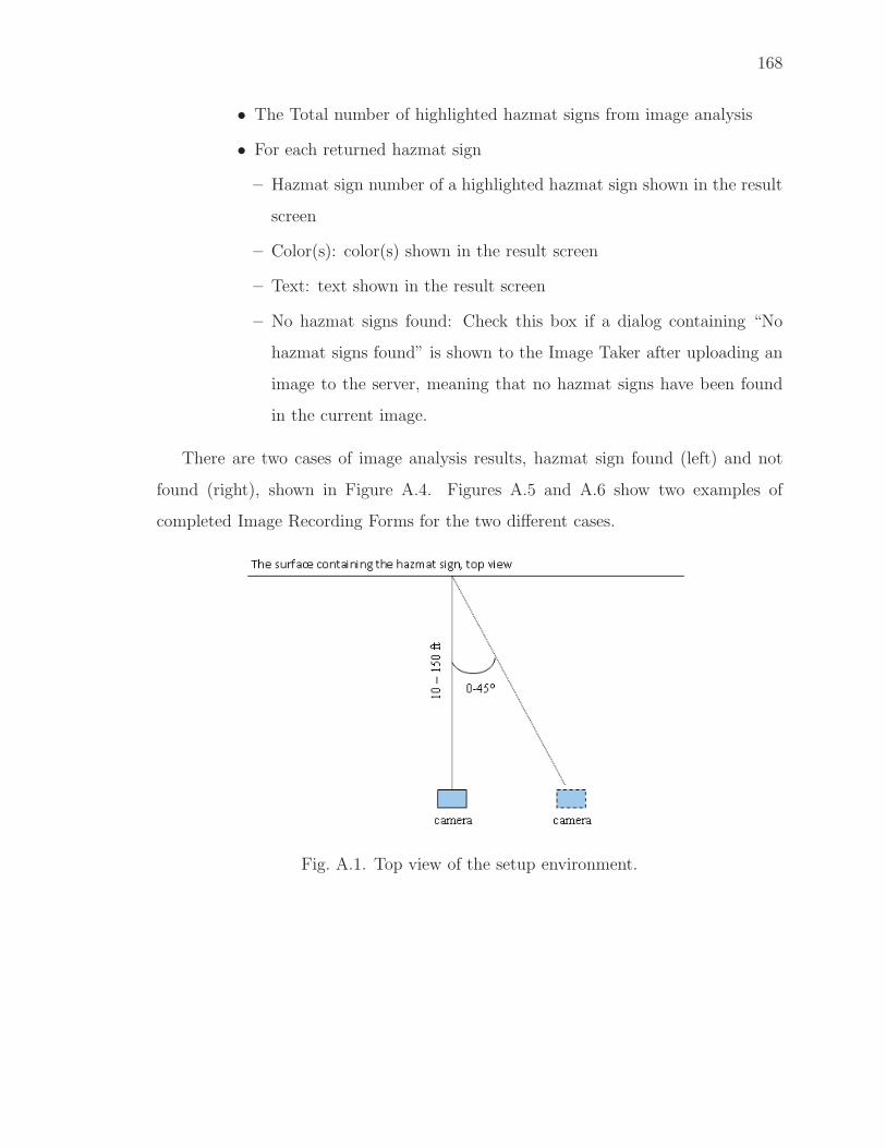
168
• The Total number of highlighted hazmat signs from image analysis
• For each returned hazmat sign
– Hazmat sign number of a highlighted hazmat sign shown in the result
screen
– Color(s): color(s) shown in the result screen
– Text: text shown in the result screen
– No hazmat signs found: Check this box if a dialog containing “No
hazmat signs found” is shown to the Image Taker after uploading an
image to the server, meaning that no hazmat signs have been found
in the current image.
There are two cases of image analysis results, hazmat sign found (left) and not
found (right), shown in Figure A.4. Figures A.5 and A.6 show two examples of
completed Image Recording Forms for the two different cases.
Fig. A.1. Top view of the setup environment.

169
Image Recording Form
Image Taker Name: ID: Affiliation:
Date: / / Starting Time: : :
Device Make: Device Model:
Ground Truth Information Angle of View ° Distance ft
Image
ID
Hazmat Sign
Number
Total Num. of
Hazmat Signs Color(s) UNID Symbol Class Text Comments
Image Analysis Results No Zoom [ ] Zoom [ ] 1/4 1/2 3/4 Full
Image
ID
Hazmat Sign
Number
Total Num. of
Hazmat Signs Color(s) UNID Symbol Class Text
No hazmat
signs found
[ ]
Fig. A.2. Image recording form for the MERGE project.

170
(a) UNID (b) Symbol (c) Class (d) Text
Fig. A.3. Hazmat sign identifiers.
Fig. A.4. Examples and screenshots of the two cases of image analysisresults, hazmat sign found (left) and not found (right).

171
Fig. A.5. Examples of completed image recording form for hazmatsign found in Figure A.4 (left).
Fig. A.6. Examples of completed image recording form for hazmatsign not found in Figure A.4 (right).

VITA

172
VITA
Bin Zhao obtained the B.S. degree in Telecommunication Engineering and the
M.S. degree in Information and Telecommunication Engineering (both with Highest
Distinction) from Xidian University, Xi’an, China. He was a Graduate Fellow and
Research Assistant of the National Key Laboratory of Integrated Service Networks
(ISN), Xi’an, China. He is pursuing the Ph.D. degree in Electrical and Computer
Engineering in Purdue University, West Lafayette, Indiana, USA. He was working as a
Graduate Teaching Assistant in the School of Electrical and Computer Engineering in
Purdue University from 2009 to 2010. He is working as a Graduate Research Assistant
in the Video and Image Processing Laboratory (VIPER) under the supervision of
Professor Edward J. Delp since 2010. He is a student member of the IEEE, the
IEEE Communications Society, and the IEEE Signal Processing Society. His research
interests include image analysis, image and video processing, computer vision, object
recognition, and machine learning.
Related Documents