PNNL-25185 RPT-IGTP-010 Rev. 0 Integrated Disposal Facility FY 2016: ILAW Evaluation of the eSTOMP Simulator May 2016 Vicky Freedman Diana Bacon Yilin Fang

Welcome message from author
This document is posted to help you gain knowledge. Please leave a comment to let me know what you think about it! Share it to your friends and learn new things together.
Transcript
PNNL-25185
RPT-IGTP-010 Rev. 0
Integrated Disposal Facility FY 2016: ILAW Evaluation of the eSTOMP Simulator
May 2016 Vicky Freedman Diana Bacon Yilin Fang
PNNL-25185 RPT-IGTP-010 Rev. 0
Integrated Disposal Facility FY 2016: ILAW Evaluation of the eSTOMP Simulator Vicky Freedman Diana Bacon Yilin Fang March 2016 Prepared for the U.S. Department of Energy under Contract DE-AC05-76RL01830 Pacific Northwest National Laboratory Richland, Washington 99352
iii
Executive Summary
This document describes two sets of simulations carried out to provide confidence in the eSTOMP simulator. In this report, the focus is on evaluating eSTOMP on a lysimeter experiment for the glassified waste, and verifying eSTOMP through a series of published benchmarks on cementitious wastes. These activities are carried out within the context of providing model confidence and support. Although eSTOMP meets safety software requirements, this designation refers to code management, documentation and testing requirements and is not directly related to terms commonly used to provide confidence in simulation codes, such as verification and validation. Whereas verification is a comparison of results among different simulators, validation is usually defined as a combination of the code and the site conceptual model, and is a measure of the model’s predictive capability. The use of the term evaluation is used in lieu of validation because the conceptual model for the lysimeter experiment is not well understood, and the standard for validation has not been met. While model evaluation for both the benchmark and lysimeter experiment entails both qualitative and quantitative comparisons of results, it is ultimately a subjective assessment.
To this end, the eSTOMP evaluation was executed by calibrating to the measured data for effluent concentrations and flow rates for the glass waste form emplaced within Hanford sediments. Not only was glass dissolution simulated, but also interactions with the near-field sediments. Problems with the manufacture of the glass meant that the parameters initially identified for glass degradation did not apply to the glass used in the lysimeter experiments, and the boron and molybdenum effluent concentrations that were used for comparison to model results represented an accelerated glass release rate. To account for the accelerated dissolution rate in the lysimeter simulations, calibration was performed using assumptions that differed from the 2005 immobilized low-activity waste performance assessment calculations. Changes in these assumptions produced a reasonable match between simulated and observed data.
In a separate effort, eSTOMP simulations were executed for five benchmark simulations published by Perko et al.1 All of the simulations included a crack within the cement, with contrasting physical and transport properties. The crack caused localized effects and also influenced the leaching process and degradation fronts. For all of the benchmark simulation cases, eSTOMP results were found to be in reasonable agreement with the results generated from other simulators.
The conclusion drawn from the benchmark publication and from the work presented in this report is that the numerical formulation of the simulators can significantly influence the results. The largest effect resulted from the kinetic formulation for solid-aqueous phase reactions used in eSTOMP, which, when using the quasi-equilibrium rate adopted by one of the other simulators in the benchmark, still showed impacts of its kinetic formulation. Only after increasing the intrinsic rate constant to more closely simulate equilibrium conditions did eSTOMP results more closely align with the predictions of the other simulators. This result underscored the importance of calibration, especially given the impacts that different numerical methods can have on the solution. Notably, eSTOMP was the only simulator that demonstrated the impact of the crack relative to the rest of the domain due to the kinetic formulation.
1 Perko J, KU Mayer, G Koskowski, L De Windt, J Govaerts, D Jacques, D Su, and JCL Meeussen. 2015. “Decalcification of cracked cement structures.” Computational Geosciences. doi:10.1007/s10596-014-9467-2.

iv
The simulations presented in this report demonstrate that eSTOMP can simulate the degradation of both glass and cementitious waste forms, as well as the coupled flow and geochemical reactions that may occur with any near-field materials influencing waste form behavior. In addition, the eSTOMP simulator can address the required process and property detail via massively parallel processing, and has been qualified as NQA-1 safety software. The results presented in this report provide confidence in the ability of eSTOMP to generate physically realistic results to support performance assessment modeling for the Integrated Disposal Facility at Hanford.
v
Acknowledgments
This work was completed as part of the ILAW Glass Testing for Disposal at IDF project. Support for this project came through Washington River Protection Solutions (WRPS). We thank Mark Rockhold (PNNL) for his technical review of the document, Guzel Tartakovsky (PNNL) for review of the calculated values used in this report, and Matt Wilburn (PNNL) for the editorial review of this report. We also wish to acknowledge Dave Swanberg, Steven Kelly, and Elvie Brown of WRPS for programmatic guidance, direction, and support.

vii
Acronyms and Abbreviations
aq aqueous
ASME American Society of Mechanical Engineers
ASTM ASTM International
DOE U.S. Department of Energy
EQL estimated quantification limit
eSTOMP exascale Subsurface Transport Over Multiple Phases (parallel computing version of computer model designated by “e”)
FEM finite element method
FVM finite volume method
FY fiscal year
GIM global implicit method
HCP hardened cement paste
IDF Integrated Disposal Facility
ILAW immobilized low-activity waste
LAW low-activity waste
MW molecular weight
NQA-1 ASME nuclear quality assurance standard
NRC U.S. Nuclear Regulatory Commission
OSM operator split method
PA performance assessment
PNNL Pacific Northwest National Laboratory
QA quality assurance
R&D research and development
SEM scanning electron microscopy
SSBench Subsurface Environmental Simulation Benchmarking
STORM Subsurface Transport Over Reactive Multiphases (computer code)
TST transition state theory
WRPS Washington River Protection Solutions
WTP Hanford Tank Waste Treatment and Immobilization Plant
WWFTP WRPS Waste Form Testing Program
XRD X-ray diffraction
viii
Units of Measure
°C temperature in degrees Celsius [T(°C) = T(K) – 273.15]
cm centimeter
d day
g gram
K kelvin
kJ kilojoules
L liter
m meter
M molarity, mole/Liter
meq milliequivalents
mL milliliter
mm millimeter
mol mole
nm nanometer
ppm parts per million
s second
vol% volume percent
micro (prefix, 10-6)
ix
Contents
Executive Summary ..................................................................................................................................... iii
Acknowledgments ......................................................................................................................................... v
Acronyms and Abbreviations ..................................................................................................................... vii
Units of Measure ........................................................................................................................................ viii
1.0 Introduction ...................................................................................................................................... 1.1
1.1 Model Evaluation .................................................................................................................... 1.1
1.1.1 Definitions .................................................................................................................. 1.1
1.1.2 Approach .................................................................................................................... 1.2
1.2 Simulation Requirements ........................................................................................................ 1.2
1.3 Purpose and Organization ....................................................................................................... 1.3
1.4 Quality Assurance ................................................................................................................... 1.3
2.0 eSTOMP Evaluation: Lysimeter Simulation Results ....................................................................... 2.1
2.1 Purpose ................................................................................................................................... 2.1
2.2 Background ............................................................................................................................. 2.1
2.2.1 Lysimeter D11 – HAN28F Glass ............................................................................... 2.1
2.2.2 Lysimeter D14 – LAWA44 Glass .............................................................................. 2.3
2.3 Simulation Input File Description ........................................................................................... 2.5
2.3.1 Grid Card ................................................................................................................... 2.5
2.3.2 Mechanical Properties, Hydraulic Properties, and Saturation Function Cards .......... 2.6
2.3.3 Aqueous and Gas Relative Permeability Cards ......................................................... 2.7
2.3.4 Solute/Porous Media Interaction Card ....................................................................... 2.7
2.3.5 Geochemistry (ECKEChem) Input Cards ................................................................ 2.10
2.4 Success Criteria ..................................................................................................................... 2.15
2.5 Simulation Results ................................................................................................................ 2.16
2.6 Discussion ............................................................................................................................. 2.18
3.0 eSTOMP Verification: Cementitious Waste Benchmark ................................................................. 3.1
3.1 Purpose ................................................................................................................................... 3.1
3.2 Simulation Description ........................................................................................................... 3.1
3.3 Benchmark Structure .............................................................................................................. 3.3
3.4 Solution Methods .................................................................................................................... 3.4
3.4.1 Numerical Methods .................................................................................................... 3.4
3.5 Success Criteria ....................................................................................................................... 3.5
3.6 Simulation Input File Description ........................................................................................... 3.6
3.6.1 Solution Control Card ................................................................................................ 3.6
3.6.2 Grid Card ................................................................................................................... 3.6
3.6.3 Rock/Soil Zonation Card ........................................................................................... 3.6
x
3.6.4 Mechanical Properties Card ....................................................................................... 3.6
3.6.5 Hydraulic Properties Card .......................................................................................... 3.8
3.6.6 Saturation Function Card ........................................................................................... 3.9
3.6.7 Aqueous Relative Permeability Card ......................................................................... 3.9
3.6.8 Solute/Porous Media Interaction Card ....................................................................... 3.9
3.6.9 Initial Conditions Card ............................................................................................... 3.9
3.6.10 Boundary Conditions Card ...................................................................................... 3.10
3.6.11 Output Control Card ................................................................................................ 3.11
3.6.12 Geochemistry (ECKEChem) Input Cards ............................................................... 3.11
3.7 Simulation Results ................................................................................................................ 3.16
3.7.1 Case 0: Conservative Tracer .................................................................................... 3.16
3.7.2 Case 1: Portlandite Dissolution – Diffusive Case .................................................... 3.17
3.7.3 Case 2: Portlandite Dissolution – Advective Case ................................................... 3.21
3.7.4 Case 3: Portlandite Dissolution – Diffusive/Advective Case with Porosity Update ..................................................................................................................... 3.25
3.7.5 Case 4: HCP Dissolution – Diffusive/Advective Case with Porosity Update ......... 3.31
3.8 Discussion ............................................................................................................................. 3.36
4.0 Discussion and Summary ................................................................................................................. 4.1
5.0 References ........................................................................................................................................ 5.1
Appendix A : eSTOMP Input File for Lysimeter D14 ............................................................................. A.1
Appendix B : Hydraulic Property Analysis of Lysimeter Backfill ............................................................B.1
Appendix C : Geochemist’s Workbench Input File for LAWA44 in Columbia River water ....................C.1
Appendix D : Geochemist Workbench Input File for Backfill in Columbia River Water ........................ D.1
Appendix E : toECKE Input File for Lysimeter D14 ................................................................................ E.1
Appendix F : Input File for Perko et al. (2015) Case 0 .............................................................................. F.1
Appendix G : Input File for Perko et al. (2015) Case 1 ............................................................................ G.1
Appendix H : Input File for Perko et al. (2015) Case 2 ............................................................................ H.1
Appendix I : Input File for Perko et al. (2015) Case 3 ................................................................................ I.1
Appendix J : Input File for Perko et al. (2015) Case 4 ............................................................................... J.1
Appendix K : toECKE Input File for Perko et al. (2015) Case 1, 2 and 3 ................................................ K.1
Appendix L : toECKE Input File for Perko et al. (2015) Case 4 ............................................................... L.1
xi
Figures
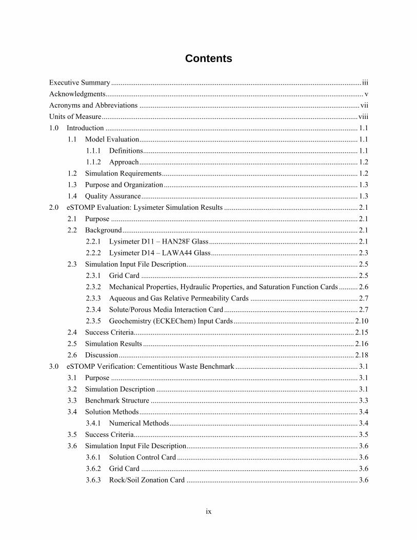
Figure 2.1. Simulated rhenium (Re) concentrations after 10 years of dissolution of small HAN-28 glass blocks surrounded by fine backfill under applied water flux of 200 mm/yr with dispersivity of 0.5 m. ............................................................................................................. 2.2
Figure 2.2. An example of the comparison between the results of chemical and transport calculations with STORM and observed releases of Re found in the drainage samples from lysimeter D11 .................................................................................................. 2.3
Figure 2.3. A comparison of the predicted and observed Mo (left) and B (right) releases for HAN-28F in lysimeter D11 ............................................................................................................. 2.3
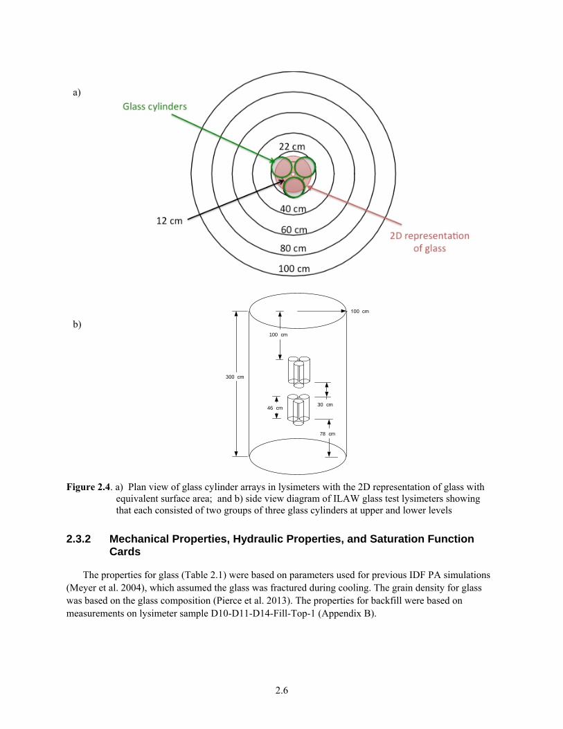
Figure 2.4. a) Plan view of glass cylinder arrays in lysimeters with the 2D representation of glass with equivalent surface area; and b) side view diagram of ILAW glass test lysimeters showing that each consisted of two groups of three glass cylinders at upper and lower levels ........................................................................................................... 2.6
Figure 2.5. Drainage from lysimeter D14 with time showing curve fit used to calculate recharge rate ......................................................................................................................................... 2.9
Figure 2.6. Comparison of measured and modeled drainage from lysimeter D14 .................................. 2.17
Figure 2.7. Comparison of measured and modeled B concentrations. D14-6 (outer diameter 12 cm), D14-5 (outer diameter 20 cm) and D14-4/7 (outer diameter 40 cm) are the innermost drainage rings, and the lines show modeled effluent concentrations at bottom radii of 1, 11.41, 21.615, and 28.145 cm, respectively. .......................................... 2.17
Figure 2.8. Comparison of measured and modeled Mo concentrations. D14-6 (outer diameter 12 cm), D14-5 (outer diameter 20 cm) and D14-4 (outer diameter 40 cm) are the innermost drainage rings, and the lines show modeled effluent concentrations at bottom radii of 1, 11.41, 21.615, and 28.145 cm, respectively. .......................................... 2.18
Figure 3.1. Benchmark simulation domain (from Perko et al. 2015) ........................................................ 3.2
Figure 3.2. Benchmark initial and boundary conditions for Cases 1–4 (from Perko et al. 2015) .............. 3.3
Figure 3.3. Mechanical properties card examples from a) Case 0 depicting a constant tortuosity for all three material types; and b) Case 3 invoking Archie’s Law for all three material types. Note the inert volume fraction is specified by the last number of each input line. ............................................................................................................................... 3.8
Figure 3.4. Excerpt from the hydraulic properties card that invokes the Kozeny-Carmen relationship for porosity and permeability. This relationship is used to update permeability based on mineral volumetric changes. ............................................................. 3.8
Figure 3.5. Comparison of dissolved tracer concentrations after 100 years along a) the horizontal profiles at y= 0.09 m from the bottom; and b) at the vertical profiles at x = 0.005 m from the center for Case 0. .................................................................................................. 3.17
Figure 3.6. Comparison of pH profiles after 100 years a) the horizontal profiles at y= 0.09 m from the bottom; and b) at the vertical profiles at x = 0.005 m from the center for Case 1. ........ 3.19
Figure 3.7. Comparison of Ca2+ profiles after 100 years a) the horizontal profiles at y= 0.09 m from the bottom; and b) at the vertical profiles at x = 0.005 m from the center for Case 1. ................................................................................................................................. 3.20
Figure 3.8. Comparison of portlandite concentrations after 100 years a) the horizontal profiles at y= 0.09 m from the bottom; and b) at the vertical profiles at x = 0.005 m from the center for Case 1. ................................................................................................................. 3.21
xii
Figure 3.9. Comparison of pH profiles after 100 years a) the horizontal profiles at y= 0.09 m from the bottom; and b) at the vertical profiles at x = 0.005 m from the center for Case 2. ........ 3.23
Figure 3.10. Comparison of Ca2+ profiles after 100 years a) the horizontal profiles at y= 0.09 m from the bottom; and b) at the vertical profiles at x = 0.005 m from the center for Case 2. ................................................................................................................................. 3.24
Figure 3.11. Comparison of portlandite concentrations after 100 years a) the horizontal profiles at y= 0.09 m from the bottom; and b) at the vertical profiles at x = 0.005 m from the center for Case 2. ................................................................................................................. 3.25
Figure 3.12. Comparison of pH profiles after 100 years a) the horizontal profiles at y= 0.09 m from the bottom; and b) at the vertical profiles at x = 0.005 m from the center for Case 3. ................................................................................................................................. 3.27
Figure 3.13. Comparison of Ca2+ profiles after 100 years a) the horizontal profiles at y= 0.09 m from the bottom; and b) at the vertical profiles at x = 0.005 m from the center for Case 3. ................................................................................................................................. 3.28
Figure 3.14. Comparison of portlandite concentrations after 100 years a) the horizontal profiles at y= 0.09 m from the bottom; and b) at the vertical profiles at x = 0.005 m from the center for Case 3. ................................................................................................................. 3.29
Figure 3.15. Comparison of porosity after 100 years a) the horizontal profiles at y= 0.09 m from the bottom; and b) at the vertical profiles at x = 0.005 m from the center for Case 3. ........ 3.30
Figure 3.16. Comparison of mineral volume fractions for a) portlandite, b) monocarboaluminate , c) calcite, d) hydrotalcite-OH, e) CSH_1.6, and f) CSH_1.2 after 100 years at vertical profiles at x = 0.005 m from the center for Case 4. ............................................... 3.32
Figure 3.17. Mineral volume fractions for all minerals at vertical profiles at x = 0.005 m from the top for Case 4 for a) eSTOMP, b) MIN3P, c) SC3K, d) HYTEC and e) SGS-GEM (Case 4) at 100 years. The eSTOMP dissolution front travels slightly faster. .................... 3.34
Figure 3.18. Mineral volume fractions for all minerals at vertical cross-section with the inert volume fraction removed at vertical profiles at x = 0.005 m from the center for Case 4 for a) eSTOMP, b) MIN3P, c) SC3K, d) HYTEC and e) OGS-GEM (Case 4) at 100 years. The eSTOMP dissolution front travels slightly faster. ....................................... 3.35
Figure 3.19. Porosity profile along the vertical profiles at x = 0.005 m from the center for Case 4. ...... 3.36
xiii
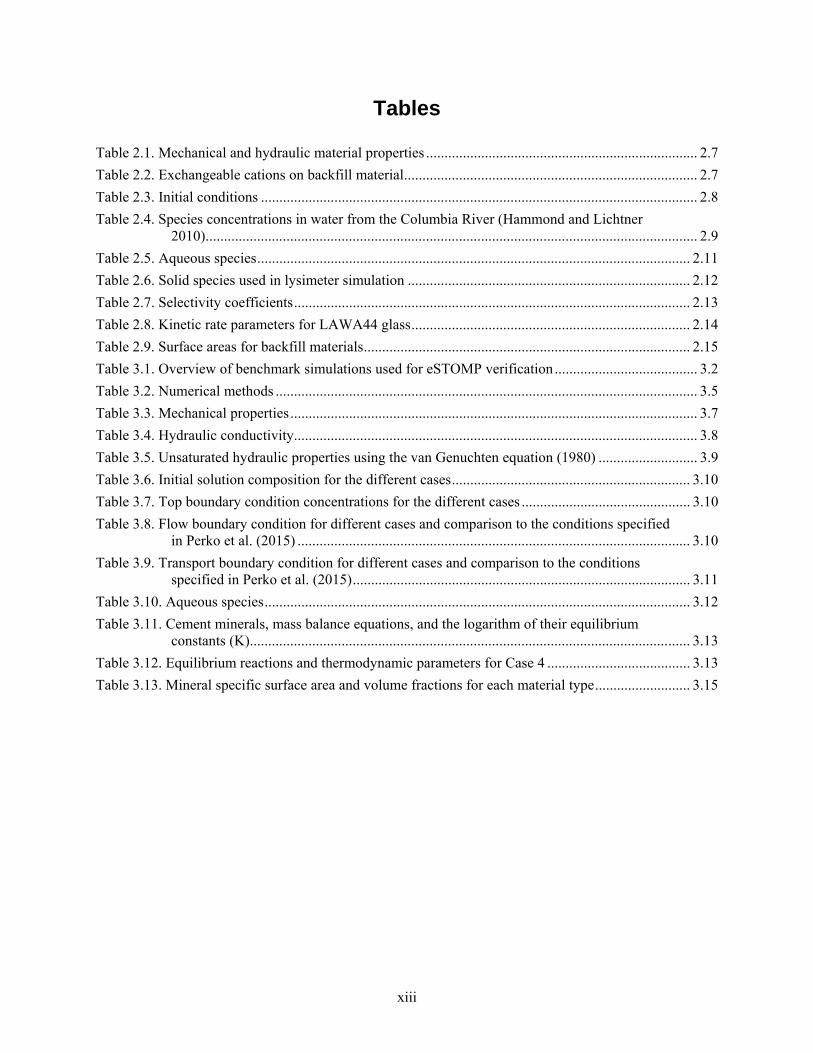
Tables
Table 2.1. Mechanical and hydraulic material properties .......................................................................... 2.7
Table 2.2. Exchangeable cations on backfill material ................................................................................ 2.7
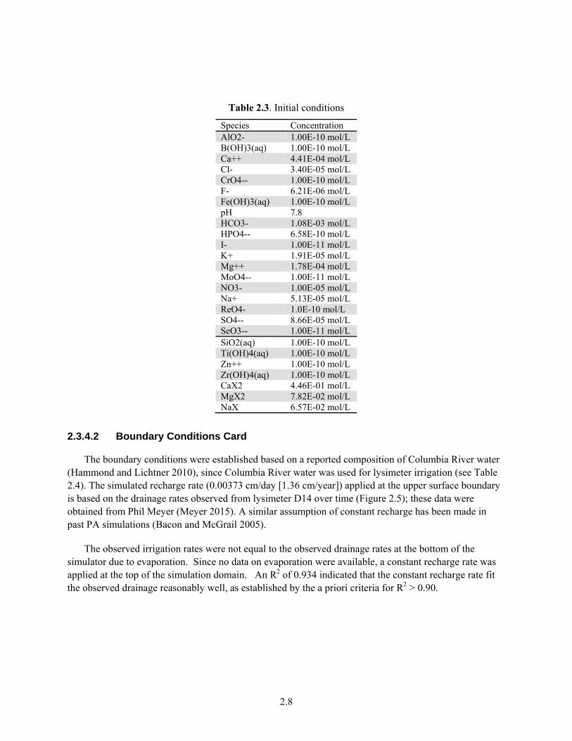
Table 2.3. Initial conditions ....................................................................................................................... 2.8
Table 2.4. Species concentrations in water from the Columbia River (Hammond and Lichtner 2010). ..................................................................................................................................... 2.9
Table 2.5. Aqueous species ...................................................................................................................... 2.11
Table 2.6. Solid species used in lysimeter simulation ............................................................................. 2.12
Table 2.7. Selectivity coefficients ............................................................................................................ 2.13
Table 2.8. Kinetic rate parameters for LAWA44 glass ............................................................................ 2.14
Table 2.9. Surface areas for backfill materials ......................................................................................... 2.15
Table 3.1. Overview of benchmark simulations used for eSTOMP verification ....................................... 3.2
Table 3.2. Numerical methods ................................................................................................................... 3.5
Table 3.3. Mechanical properties ............................................................................................................... 3.7
Table 3.4. Hydraulic conductivity .............................................................................................................. 3.8
Table 3.5. Unsaturated hydraulic properties using the van Genuchten equation (1980) ........................... 3.9
Table 3.6. Initial solution composition for the different cases ................................................................. 3.10
Table 3.7. Top boundary condition concentrations for the different cases .............................................. 3.10
Table 3.8. Flow boundary condition for different cases and comparison to the conditions specified in Perko et al. (2015) ........................................................................................................... 3.10
Table 3.9. Transport boundary condition for different cases and comparison to the conditions specified in Perko et al. (2015) ............................................................................................ 3.11
Table 3.10. Aqueous species .................................................................................................................... 3.12
Table 3.11. Cement minerals, mass balance equations, and the logarithm of their equilibrium constants (K)........................................................................................................................ 3.13
Table 3.12. Equilibrium reactions and thermodynamic parameters for Case 4 ....................................... 3.13
Table 3.13. Mineral specific surface area and volume fractions for each material type .......................... 3.15
1.1
1.0 Introduction
Subsurface flow simulations are a key component in the design and optimization of the Integrated Disposal Facility (IDF) at the Hanford Site in southeastern Washington State. Modeling and simulation can be used to explore the IDF design and inform risk as part of the performance assessment (PA) process. Although the eSTOMP (Fang et al. 2015; White and Oostrom 2000) simulator has recently been qualified as safety software and approved for use in the IDF PA, formal evaluation of the simulator is needed to provide further confidence in simulation results. Although eSTOMP is managed as NQA-1 software (see Section 1.4), this designation does not mean that the code has been ‘validated’, since the definition of validation is a combination of both the code and the site conceptual model (see Section 1.1.1).
1.1 Model Evaluation
1.1.1 Definitions
This document describes two sets of simulations carried out to provide further confidence in the eSTOMP simulator. Within the context of this document, verification is defined as the process of determining that a model implementation and its associated data accurately represent the developer’s conceptual description and specifications. With respect to process-based numerical models, verification frequently refers to comparing numerical simulation results to analytical solutions (de Marsily et al. 1992; Oreskes et al. 1994). However, for coupled processes, analytical solutions are often non-existent. Although in theory models can be verified, they cannot be verified in practice unless an exact analytical solution exists for the problem at hand (Konikow and Bredehoeft 1992). Hence, benchmarking may be used instead, which refers to the process of comparing results from two or more numerical models for the same simulation codes (Liu and Narasimhan 1989). This problem may be hypothetical or based on actual experiments. In the latter case, the comparison represents both a benchmark and a validation test, because it is based on measured data.
The term model validation has been used to provide ground-truthing for when both the conceptual model and the computer code provide a good representation of the actual processes within in the real system (IAEA 1982). However, the term validation often introduces polemic in its meaning and interpretation, as occurred in In Konikow and Bredehoft’s (1992) landmark paper on model validation that asserted that ground water models cannot be validated. A historical definition of model validation has included the process of obtaining assurance that the model reflects the behavior of the real world (NRC 1986; DOE 1986). Schlesinger (1979) provides a different interpretation by describing validation as providing substantial proof that a model has a range of accuracy. Although all of these definitions of model validation have merit, the use of this term is avoided altogether in this document, and is replaced with the term model evaluation. This is based on the National Research Council (NRC 2007) and the U.S. Environmental Protection Agency (EPA, 2009) guidance that recognizes model evaluation as a process of assessing whether a model is suitable for its intended purpose, builds confidence in model applications and increases the understanding of model strengths and limitations. Whereas “valid” may be useful in describing the processes represented in a model, it prejudices expectations toward a positive outcome. The term evaluation is recognized as a more neutral term when referring to what may be expected of the outcome (NRC 2007).
1.2
1.1.2 Approach
Model evaluation for the glass lysimeter experiments is carried out by demonstrating that the model is capable of making “sufficiently accurate” simulations (Refsgaard 1997). However, assessments of “sufficiently accurate” can be subjective. For example, two principal views on this subject are presented in Konikow and Bredehoft’s (1992) paper. The first is called positivism and argues that theories are confirmed or refuted on the basis of critical experiments designed for that purpose (Matalas et al. 1982). Clearly, this view is closely aligned with the goals of the lysimeter experiments; that is to demonstrate the behavior of the glass waste forms when emplaced within near-field sediments, and to simulate it with sufficient accuracy. The second view, however, argues the opposite, and holds that scientists cannot validate a hypothesis, only invalidate it (Popper 1959). Within this context, the concept of sufficiently accurate is subjective, since it relies on expert judgment and the model application.
Data limitations exist for the glass lysimeter simulations. Laboratory data supporting glass dissolution rates do not align with the field experimental conditions. This severely limits the model evaluation, but still provides value by demonstrating eSTOMP’s ability to simulate waste form interactions with near-field materials and subsequent transport to the bottom of the lysimeter. Hence, success in model evaluation is defined as agreement between eSTOMP predictions and lysimeter measurements of water drainage rates from the bottom of the lysimeter, and effluent concentrations at select times.
The evaluation for cementitious waste forms is carried out by comparing eSTOMP results to results generated from other simulators. Inherent in this approach is a known solution, with a range given by the other simulators. Metrics used for comparison are also given by the benchmarks published in Perko et al. (2015). Although this is more structured than the model evaluation for the glass lysimeter experiment, the evaluation is still a qualitative assessment. As stated in the introduction to the Special Issue (Steefel et al. 2015), the intent of the benchmarks was to develop simulator conformance with norms established by the subsurface science and engineering community. Achieving a common solution was the primary goal, although a range of solutions was anticipated.
Within this context, this report presents support for evaluating eSTOMP for simulating the degradation of both glass and cementitious waste forms that are to be emplaced within the IDF repository. Arguments are provided that support this evaluation, recognizing that the assessment is subjective.
1.2 Simulation Requirements
To simulate the range in possible performance for waste forms emplaced in the IDF, the simulator must be able to integrate 1) characterized properties for waste form, waste package, and sediments; 2) identified system of reactions, thermodynamics, and rates; 3) knowledge from laboratory and field experiments; 4) required flow, transport, and multicomponent reaction processes; and 5) subsurface conditions to forecast the waste form degradation and the release of contaminants of concern for 10,000 years or more. The simulator capabilities should include multiphase (gas and liquid) flow, dual-porosity modeling for fractures and matrix, and multicomponent reactive transport with feedback to flow due to changes in mineral volume fractions. For the most comprehensive and detailed 3D coupled-process, field-scale modeling scenarios, single-processing-node workstations will not be able to address the large memory and computational requirements.
1.3
The eSTOMP simulator can address the required process and property detail via massively parallel processing, and has been qualified as NQA-1 safety software. The ability of eSTOMP to simulate coupled, mechanistically detailed processes enables a more realistic representation of the conceptual model without compromising dimensionality, resolution, process, or property detail to make the run times tractable. If simple models are to be used for PA modeling, simulation results from the more mechanistically based eSTOMP reactive transport model can be used to provide the technical basis for model abstraction.
The simulation of relevant and realistically complex problems is especially important to the qualification of coupled-process simulators if they are to be used for the IDF PA. Cement-based benchmarks requiring varying degrees of sophistication are now available, developed primarily in collaboration with international teams who are involved in safety assessments of subsurface radioactive waste repositories. Members of the eSTOMP modeling team have convened and participated in the development and publication of these benchmarks through a series of Subsurface Environmental Simulation Benchmarking (SSBench) workshops (Berkeley, USA in 2011; Taipei, China in 2012; Leipzig, Germany in 2013; Cadarache, France in 2014) that included modeling teams from Australia, Belgium, Canada, China, France, Germany, Korea, Netherlands, Spain, Switzerland, Taiwan, and the U.S. (Steefel et al. 2015). A special issue of the Journal of Computational Geosciences was published in 2015 with several reactive transport benchmarks, some of which are relevant to the Cast Stone IDF PA (Perko et al. 2015).
1.3 Purpose and Organization
The purpose of this report is to provide the simulation results that further support the use of the eSTOMP simulator for use on the IDF PA. Section 2.0 presents simulation results from field tests conducted for approximately 8 years with immobilized low-activity waste (ILAW) glass samples in a lysimeter facility on the Hanford Site (Meyer et al. 2001). Section 3.0 describes the verification problem for a cementitious waste form, based on a benchmark problem published by Perko et al. (2015). Section 4.0 summarizes the reported results. Section 5.0 provides a list of references, and the appendices that provide a listing of input files and data.
1.4 Quality Assurance
This work was conducted with funding from Washington River Protection Solutions (WRPS) under contract 36437-161, ILAW Glass Testing for Disposal at IDF. The work was conducted as part of Pacific Northwest National Laboratory (PNNL) Project 66309, ILAW Glass Testing for Disposal at IDF.
All research and development (R&D) work at PNNL is performed in accordance with PNNL’s laboratory-level Quality Management Program, which is based on a graded application of NQA-1-2000, Quality Assurance Requirements for Nuclear Facility Applications, to R&D activities. In addition to the PNNL-wide quality assurance (QA) controls, the QA controls of the WRPS Waste Form Testing Program (WWFTP) QA program were also implemented for the work.
The WWFTP QA program consists of the WWFTP Quality Assurance Plan (QA-WWFTP-001) and associated QA-NSLW-numbered procedures that provide detailed instructions for implementing NQA-1 requirements for R&D work. The WWFTP QA program is based on the requirements of NQA-1-2008,
1.4
Quality Assurance Requirements for Nuclear Facility Applications, and NQA-1a-2009, Addenda to ASME NQA-1-2008 Quality Assurance Requirements for Nuclear Facility Applications, graded on the approach presented in NQA-1-2008, Part IV, Subpart 4.2, “Guidance on Graded Application of Quality Assurance (QA) for Nuclear-Related Research and Development.”
Simulations executed and documented this report were assigned the technology level “Applied Research” and were conducted in accordance with procedure QA-NSLW-1102, Scientific Investigation for Applied Research. All staff members contributing to the work have technical expertise in the subject matter and received QA training prior to performing quality-affecting work. The “Applied Research” technology level provides adequate controls to ensure that the activities were performed correctly. Use of both the PNNL-wide and WWFTP QA controls ensured that all client QA expectations were addressed in performing the work.
2.1
2.0 eSTOMP Evaluation: Lysimeter Simulation Results
2.1 Purpose
Performance assessment calculations for ILAW glass to be disposed of at the Hanford Site depend on simulations of long-term glass corrosion behavior and contaminant transport that are being performed via reactive chemical transport modeling (e.g., eSTOMP simulations). Confidence in the underlying physical and geochemical processes that are being simulated by such conceptual models and computer codes can be significantly enhanced through carefully controlled field testing (Wicks 2001). Field testing allows the IDF PA program to obtain independent and site-relevant data on glass corrosion at temperature conditions relevant to the actual disposal system, since glass corrosion rates are accelerated using elevated temperatures in the laboratory. Moreover, the impact of near-field sediments on corrosion rates and the impact of in-situ moisture conditions can also be better represented in the field. However, data on interactions with near-field sediments were not collected, and moisture conditions were higher than what is anticipated at the IDF protected with a barrier. Nonetheless, these data can be used to evaluate the models used to forecast the long-term behavior of the glass waste form as they provide additional information on actual (and potential) conditions at the repository.
The work presented in this section focuses on evaluating eSTOMP, using data from field tests conducted for approximately 7 years with ILAW glass samples in a lysimeter facility on the Hanford Site (Meyer et al. 2001). A list of these data is provided in Appendix B. This evaluation provides confidence that eSTOMP is producing reasonable estimates of glass corrosion rates and releases of contaminants of concern.
2.2 Background
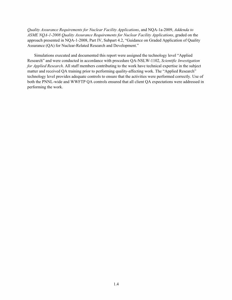
In 2002, before the lysimeter experiment was begun, preliminary simulations of expected HAN28F waste form degradation during the experiment were conducted (Meyer et al. 2001). These simulations were conducted using version 2 of the STORM simulator, as shown in Figure 2.1 (Bacon et al. 2000). The preliminary simulations were executed to establish the anticipated corrosion rates.
The glass corrosion was simulated using the anticipated field experimental conditions, using the non-radioactive rhenium (Re) as a surrogate for the radioactive technetium (Tc) to be sequestered in the glass. Rhenium was used due to the similarities in chemistry. Under oxidizing conditions, both Re and Tc have a minimal tendency to sorb to soil minerals, and persist in the environment as anions in the +7 oxidation state, i.e., pertechnetate (TcO4
-) and perrhenate (ReO4-). Both Tc and Re are subject to chemical reduction
to the +4 oxidation state, which is far less soluble and mobile in the environment.
2.2.1 Lysimeter D11 – HAN28F Glass
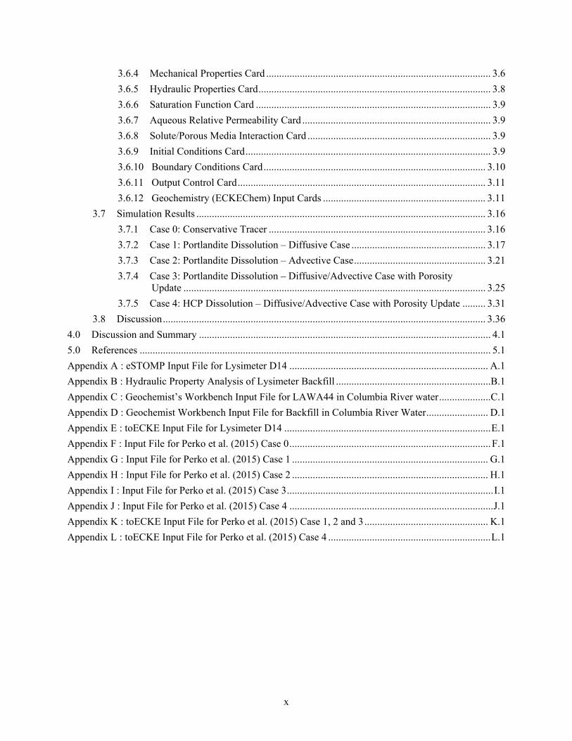
In 2009, model results were compared to observed data from the D11 lysimeter drainage containing the HAN28F glass (Strachan 2009). Because the soil hydraulic properties and recharge rates used in the preliminary STORM calculations from 2002 did not accurately reflect the lysimeter conditions, model predictions did not match the observed effluent concentrations. Recharge rates used in the Strachan (2009) simulations were 50 and 200 mm/yr, although the actual recharge rates at the lysimeter facility
2.2
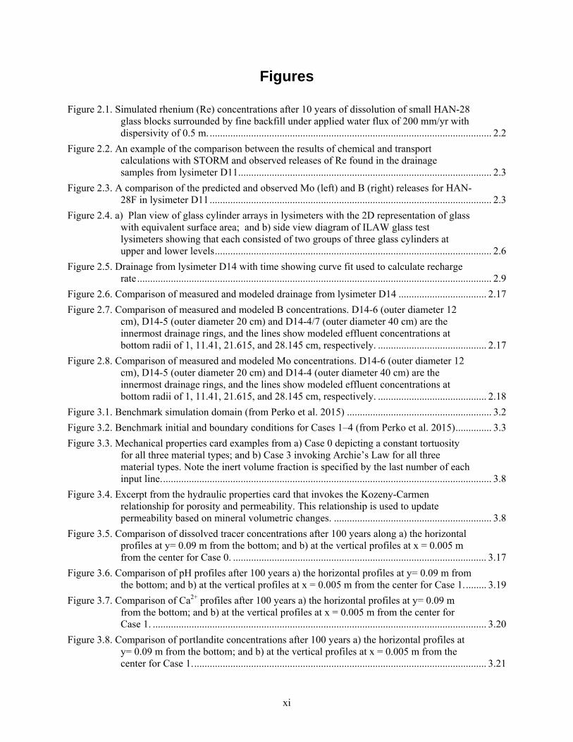
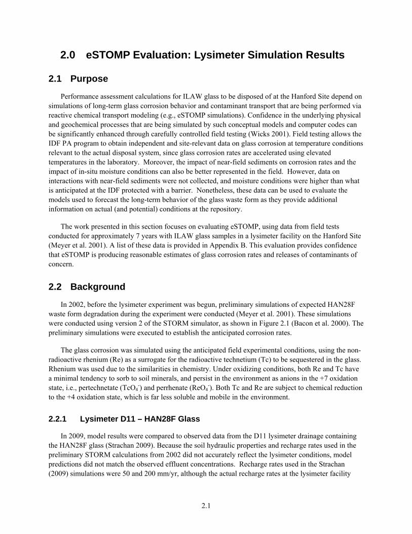
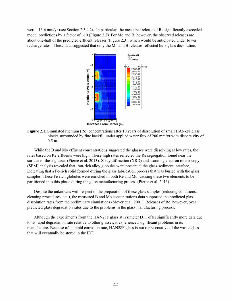
were ~13.6 mm/yr (see Section 2.3.4.2). In particular, the measured release of Re significantly exceeded model predictions by a factor of ~10 (Figure 2.2). For Mo and B, however, the observed releases are about one-half of the predicted effluent releases (Figure 2.3), which would be anticipated under lower recharge rates. These data suggested that only the Mo and B releases reflected bulk glass dissolution.
Figure 2.1. Simulated rhenium (Re) concentrations after 10 years of dissolution of small HAN-28 glass blocks surrounded by fine backfill under applied water flux of 200 mm/yr with dispersivity of 0.5 m.
While the B and Mo effluent concentrations suggested the glasses were dissolving at low rates, the rates based on Re effluents were high. These high rates reflected the Re segregation found near the surface of these glasses (Pierce et al. 2013). X-ray diffraction (XRD) and scanning electron microscopy (SEM) analysis revealed that iron-rich alloy globules were present at the glass-sediment interface, indicating that a Fe-rich solid formed during the glass fabrication process that was buried with the glass samples. These Fe-rich globules were enriched in both Re and Mo, causing these two elements to be partitioned into this phase during the glass manufacturing process (Pierce et al. 2013).
Despite the unknowns with respect to the preparation of these glass samples (reducing conditions, cleaning procedures, etc.), the measured B and Mo concentrations data supported the predicted glass dissolution rates from the preliminary simulations (Meyer et al. 2001). Releases of Re, however, over predicted glass degradation rates due to the problems in the glass manufacturing process.
Although the experiments from the HAN28F glass at lysimeter D11 offer significantly more data due to its rapid degradation rate relative to other glasses, it experienced significant problems in its manufacture. Because of its rapid corrosion rate, HAN28F glass is not representative of the waste glass that will eventually be stored in the IDF.
Distance From Center (m)
He
igh
tA
bo
veB
ott
om
(m)
0 0.25 0.5 0.75 10
0.5
1
1.5
2
2.5
3
ReO4- (moles/kg)2.76E-072.58E-072.39E-072.21E-072.02E-071.84E-071.66E-071.47E-071.29E-071.10E-079.20E-087.36E-085.52E-083.68E-081.84E-08
Fine Backfill10 yr200 mm/yr
2.3
Figure 2.2. An example of the comparison between the results of chemical and transport calculations with STORM and observed releases of Re found in the drainage samples from lysimeter D11
Figure 2.3. A comparison of the predicted and observed Mo (left) and B (right) releases for HAN-28F in lysimeter D11
2.2.2 Lysimeter D14 – LAWA44 Glass
In 2003, experiments were initiated with the LAWA44 waste glass in lysimeter D14, and executed for a period of 7 years. The LAWA44 glass dissolves more slowly than the HAN28F glass, which means that fewer data were collected. However, the LAWA44 glass formulation represents glass waste that will be stored in the IDF, and as a result, has been used as the base case glass for previous PA simulations (Bacon and McGrail 2005).
The LAWA44 glass prepared for the lysimeter experiments was subject to the same manufacturing problems described for HAN28F (Pierce et al. 2013). B, Mo, and Re were the only glass-specific species identified in effluent samples taken from lysimeter D14 (Meyer 2015). Other tracer species added to the glass, including iodine and selenium, were not observed in the effluent samples analyzed (Meyer 2015). As with the HAN28F experiments in lysimeter D11, B, Mo, and Re pore water leachate concentrations were thought to be higher than would be predicted by bulk dissolution of the glass (Pierce et al. 2013). A further problem was that there was a large number of non-detects (concentrations below the detection limit), leaving just a few measurements for comparison (Meyer 2015). Despite these difficulties, it was
Time, y
0 1 2 3 4
Re
Rel
ease
, g
0.0
0.2
0.4
0.6
0.8
Predicted - 200 mm/y 50 mm/y
Observed
Time, y
0 1 2 3 4
Mo
Re
leas
e, m
g
0.0
10.0
20.0
30.0
40.0
50.0
Predicted - 200 mm/y 50 mm/y
Observed
Time, y
0 1 2 3 4
B R
elea
se, g
0.0
0.1
0.2
0.3
0.4
Predicted - 200 mm/y 50 mm/y
Observed
2.4
assumed that, as in the HAN28F experiments, B and Mo might be more indicative of bulk dissolution of the glass than Re, and these species were chosen for comparison with modeled results.
2.2.2.1 Soil Water Extracts – Lysimeters D10, D11, D14
In FY 2012, experimental data were collected to identify the elemental concentration profiles for three lysimeters to determine the flux of elements from the glass samples as a function of depth (Pierce et al. 2013). This was accomplished with 1:1 water extracts on sediment samples collected from sediment cores taken from the lysimeters. Surface analysis of a select number of glass samples collected from the lysimeter facility was carried out using SEM and XRD analyses.
In FY 2014, geochemical modeling of the water extracts was conducted to verify the applicability of the currently used suite of secondary phases (Cantrell 2014). This work consisted of conducting saturation index calculations on the 1:1 water extracts and/or pore-water extractions of sediment samples collected from sediment cores taken from the lysimeters. The SEM and XRD results were used to verify the presence of phases identified in the geochemical modeling.
Only two detectable measurements of B were recorded for the soil water extracts. Also, since they were 1:1 water extracts, they did not represent actual pore water concentrations. Furthermore, effluent contaminant fluxes, not pore-water concentrations, are the performance objective for the PA (Mann et al. 2001). For these reasons, the soil-water extract data will not be used in the model evalution.
2.2.2.2 Glass Selection for Evaluation
Both the LAWA44 and HAN28F glasses were considered for eSTOMP evaluation. Because the HAN28F is a fast-dissolving glass, a large number of time-dependent measurements were available for comparison to simulated results. By contrast, the LAWA44 glass dissolved much more slowly, and fewer data were available for comparison. The initial goal was to include both glasses in the evaluation, and simulate the experiments at both lysimeter D-10 (HAN28F) and lysimeter D-14 (LAWA44). The benefit of simulating the dissolution of the HAN28F glass was the rich data set, whereas the benefit of the LAWA44 glass was that it represented a targeted glass for the WTP.
For both glasses, issues with the manufacture of the glass occurred. Both were placed in graphite crucibles that created reducing conditions, creating preferential precipitation of Re and Mo on the outer portion of the glass. Hence, the glass emplaced in the lysimeter was not the same as the glass used in laboratory experiments to identify rate parameters. Given the lack of data on the actual glass compositions and dissolution rates, the approach to the evaluation was to simulate the glass degradation using the data on glass composition from laboratory experiments because this was the only data available for parameterizing the model. This meant that calibration would be needed to match apparent or accelerated dissolution rates.
The simulations for both the HAN28F and LAWA44 followed the same procedures, as outlined in Section 2.3. However, only the LAWA44 glass evaluation case is documented in this report due to numerical instabilities that occurred during the HAN28F experiments. The numerical instabilities and convergence difficulties were associated with the high rates of dissolution. This is a common problem encountered when simulating reactive transport, since the numerical treatment of the large rates leads to a stiff matrix that can be difficult and impractical to solve due to small time-step requirements. Testing
2.5
with the STOMP (White and Oostrom 2000; White et al. 2015) simulator showed that it experienced the same numerical instabilities and convergence failures as eSTOMP. Modeling the HAN28F lysimeter experiments would have required more time than afforded in this effort, as iteration between batch and reactive transport modeling was required to identify secondary mineral precipitates forming under the high rates of dissolution. Hence, the evaluation focused on the experiments with the LAWA44 glass not only because it is a realistic target for the WTP, but because it was also used in the 2001 and 2005 Integrated Disposal Facility Performance Assessments (PA), and is considered in the current PA.
2.3 Simulation Input File Description
The objective of the eSTOMP evaluation is to simulate the experiment conditions in lysimeter D14, comparing predicted concentrations of selected glass species (B and Mo) in the effluent. Lysimeter D14 contained LAWA44 glass samples (Pierce et al. 2013).
A listing of the eSTOMP input file for Lysimeter D14 is given in Appendix A. The sources of data for each input card are described in the following sections. Model input parameters from previous PA simulations (Bacon and McGrail 2005) were used unless experimental data were available.
The eSTOMP input file is divided into sections called cards. Each card used in this work is described in the sections that follow.
2.3.1 Grid Card
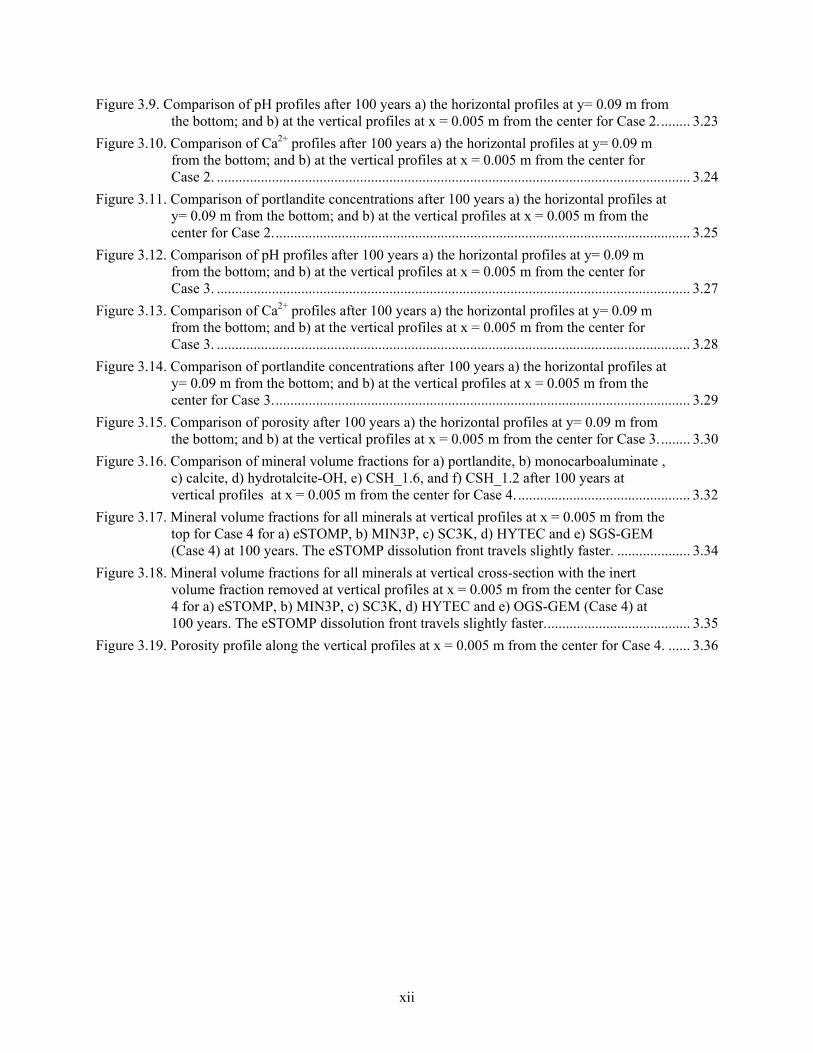
The model grid is based on the lysimeter schematic shown in Figure 2.4 (Pierce et al. 2013), which shows the different radii at the lysimeter facility (Figure 2.4a). A side-view image of the lysimeter is also shown in Figure 2.4b. Based on the experimental setup, a 2D radial grid was constructed, rather than a full 3D grid, to accelerate run times. Because the horizontal breaks between each waste package cannot be represented in a 2D radial grid, and the release rate from the glass is proportional to the exposed surface area of the glass, the 2D grid was constructed by assuming that a cylindrical ring of glass with the same surface area represents each cluster of three waste packages (see Figure 2.4a). Given that each waste package had a height of 46 cm and a radius of 10 cm, this yields a total surface area of ~942 cm2 for the three canisters. In two dimensions, the glass waste packages are represented by a cylindrical ring with an inner radius of 1 cm and an outer radius of 17.35 cm, yielding the same total surface area of the glass buried in lysimeter D14. This resulted in a 31 59 cell grid, with vertical grid spacing varying from 5 to 5.2 cm, and horizontal grid spacing varying from 1 cm in the center (left side) to 5 cm on the outside (right side).
2.6
Figure 2.4. a) Plan view of glass cylinder arrays in lysimeters with the 2D representation of glass with equivalent surface area; and b) side view diagram of ILAW glass test lysimeters showing that each consisted of two groups of three glass cylinders at upper and lower levels
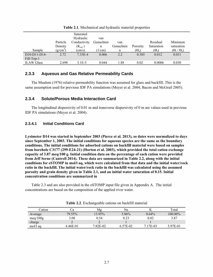
2.3.2 Mechanical Properties, Hydraulic Properties, and Saturation Function Cards
The properties for glass (Table 2.1) were based on parameters used for previous IDF PA simulations (Meyer et al. 2004), which assumed the glass was fractured during cooling. The grain density for glass was based on the glass composition (Pierce et al. 2013). The properties for backfill were based on measurements on lysimeter sample D10-D11-D14-Fill-Top-1 (Appendix B).
300 cm
100 cm
30 cm
100 cm
46 cm
78 cm
a)
b)
2.7
Table 2.1. Mechanical and hydraulic material properties
Sample
Particle Density (g/cm3)
Saturated Hydraulic
Conductivity (Ksat ) (cm/s)
van Genuchten
α (1/cm)
van Genuchten
nPorosity
(Θs)
Residual Saturation
(Θr)
Minimum saturation (Θr / Θs)
D10-D11-D14-Fill-Top-1
2.72 7.33E-4 0.006 2.2 0.385 0.012 0.031
ILAW Glass 2.698 3.1E-5 0.044 1.88 0.02 0.0006 0.030
2.3.3 Aqueous and Gas Relative Permeability Cards
The Mualem (1976) relative permeability function was assumed for glass and backfill. This is the same assumption used for previous IDF PA simulations (Meyer et al. 2004; Bacon and McGrail 2005).
2.3.4 Solute/Porous Media Interaction Card
The longitudinal dispersivity of 0.01 m and transverse dispersivity of 0 m are values used in previous IDF PA simulations (Meyer et al. 2004).
2.3.4.1 Initial Conditions Card
Lysimeter D14 was started in September 2003 (Pierce et al. 2013), so dates were normalized to days since September 1, 2003. The initial conditions for aqueous species are the same as the boundary conditions. The initial conditions for adsorbed cations on backfill material were based on samples from borehole C3177 (299-E24-21) (Horton et al. 2003), which provided the total cation exchange capacity of 3.87 meq/100 g. Initial condition data on the percentage of each cation were provided from Jeff Serne (Cantrell 2014). These data are summarized in Table 2.2, along with the initial conditions for eSTOMP in mol/l aq, which were calculated from that data and the initial water/rock ratio in the backfill. The initial water/rock ratio in the backfill was calculated using the assumed porosity and grain density given in Table 2.1, and an initial water saturation of 0.15. Initial concentration conditions are summarized in
Table 2.3 and are also provided in the eSTOMP input file given in Appendix A. The initial concentrations are based on the composition of the applied river water.
Table 2.2. Exchangeable cations on backfill material
Cation Ca Mg Na K Total Average 79.55% 13.95% 5.86% 0.64% 100.00% meq/100g 3.08 0.54 0.23 0.02 3.87 charge 2 2 1 1 mol/l aq 4.46E-01 7.82E-02 6.57E-02 7.17E-03 5.97E-01
2.8
Table 2.3. Initial conditions
Species Concentration AlO2- 1.00E-10 mol/L B(OH)3(aq) 1.00E-10 mol/L Ca++ 4.41E-04 mol/L Cl- 3.40E-05 mol/L CrO4-- 1.00E-10 mol/L F- 6.21E-06 mol/L Fe(OH)3(aq) 1.00E-10 mol/L pH 7.8 HCO3- 1.08E-03 mol/L HPO4-- 6.58E-10 mol/L I- 1.00E-11 mol/L K+ 1.91E-05 mol/L Mg++ 1.78E-04 mol/L MoO4-- 1.00E-11 mol/L NO3- 1.00E-05 mol/L Na+ 5.13E-05 mol/L ReO4- 1.0E-10 mol/L SO4-- 8.66E-05 mol/L SeO3-- 1.00E-11 mol/L SiO2(aq) 1.00E-10 mol/L Ti(OH)4(aq) 1.00E-10 mol/L Zn++ 1.00E-10 mol/L Zr(OH)4(aq) 1.00E-10 mol/L CaX2 4.46E-01 mol/L MgX2 7.82E-02 mol/L NaX 6.57E-02 mol/L
2.3.4.2 Boundary Conditions Card
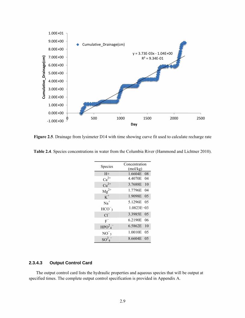
The boundary conditions were established based on a reported composition of Columbia River water (Hammond and Lichtner 2010), since Columbia River water was used for lysimeter irrigation (see Table 2.4). The simulated recharge rate (0.00373 cm/day [1.36 cm/year]) applied at the upper surface boundary is based on the drainage rates observed from lysimeter D14 over time (Figure 2.5); these data were obtained from Phil Meyer (Meyer 2015). A similar assumption of constant recharge has been made in past PA simulations (Bacon and McGrail 2005).
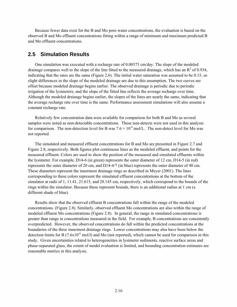
The observed irrigation rates were not equal to the observed drainage rates at the bottom of the simulator due to evaporation. Since no data on evaporation were available, a constant recharge rate was applied at the top of the simulation domain. An R2 of 0.934 indicated that the constant recharge rate fit the observed drainage reasonably well, as established by the a priori criteria for R2 > 0.90.
2.9
Figure 2.5. Drainage from lysimeter D14 with time showing curve fit used to calculate recharge rate
Table 2.4. Species concentrations in water from the Columbia River (Hammond and Lichtner 2010).
Species Concentration (mol/kg)
H+ 1.6604E�08
Ca2+ 4.4070E�04
Cu2+ 3.7688E�10
Mg2+ 1.7796E�04
K+ 1.9098E�05
Na+ 5.1296E�05
HCO−3 1.0823E−03
Cl− 3.3985E�05
F− 6.2190E�06
HPO24− 6.5862E�10
NO−3 1.0010E�05
SO24− 8.6604E�05
2.3.4.3 Output Control Card
The output control card lists the hydraulic properties and aqueous species that will be output at specified times. The complete output control specification is provided in Appendix A.
y = 3.73E‐03x ‐ 1.04E+00R² = 9.34E‐01
‐1.00E+00
0.00E+00
1.00E+00
2.00E+00
3.00E+00
4.00E+00
5.00E+00
6.00E+00
7.00E+00
8.00E+00
9.00E+00
1.00E+01
0 500 1000 1500 2000 2500
Cumulative_D
rainage(cm)
Day
Cumulative_Drainage(cm)
2.10
2.3.4.4 Surface Flux Card
The surface flux card specifies that the instantaneous and cumulative flux of B and Mo across the lower boundary of the lysimeter model will be output at each model time step.
2.3.5 Geochemistry (ECKEChem) Input Cards
The toECKE pre-processor builds many of the reactive transport input cards needed to execute simulations with the ECKEChem geochemistry module in eSTOMP. The toECKE input file is shown in Appendix E.
Prior to executing the toECKE pre-processor, the geochemical database was modified so that the thermodynamic database would be in agreement with experimental glass dissolution data, as reported in Pierce (2004). The thermo.com.V8.R6+.dat database (from Geochemist’s Workbench©) was modified using the procedures outlined in the eSTOMP quality assurance program. This created a new database named thermo.com.V8.R6+_lysimeter.dat, which was used to generate the geochemical inputs used in this work.
2.3.5.1 Aqueous Species Card
The aqueous species given in Table 2.5 were based on Geochemist’s Workbench simulations of the dissolution of glass and backfill materials. The Geochemist’s Workbench input file for LAWA44 glass dissolution is given in Appendix C. The Geochemist’s Workbench input file for backfill dissolution in Columbia River water is also provided in Appendix D. The formatted aqueous species card is provided in Appendix A. The effective diffusion coefficient was calculated using a power function model for backfill used in previous PAs (Meyer et al. 2004) given as
(2.1)
where
θ = volumetric water content (m3/m3)
De = effective diffusion coefficient (m2/s)
Dm = molecular diffusion coefficient (m2/s)
a, b = empirical fitting coefficients (dimensionless)
The power function model uses parameters of 1.84e-5 cm2/s for molecular diffusion, and fitting coefficients A = 1.486 and B = 1.956. Although eSTOMP (and STOMP) include the power function model, it does not vary by material type as implemented in STORM, and so the recommended diffusion coefficient model recommended by Meyer et al. (2004) for glass was not implemented.
2.11
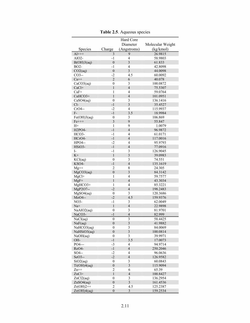
Table 2.5. Aqueous species
Species Charge
Hard Core Diameter
(Angstroms) Molecular Weight
(kg/kmol) Al+++ 3 9 26.9815 AlO2- -1 4 58.9803 B(OH)3(aq) 0 3 61.833 BO2- -1 4 42.8098 CO2(aq) 0 3 44.0098 CO3-- -2 4.5 60.0092 Ca++ 2 6 40.078 CaCO3(aq) 0 3 100.0872 CaCl+ 1 4 75.5307 CaF+ 1 4 59.0764 CaHCO3+ 1 4 101.0951 CaSO4(aq) 0 3 136.1416 Cl- -1 3 35.4527 CrO4-- -2 4 115.9937 F- -1 3.5 18.9984 Fe(OH)3(aq) 0 3 106.869 Fe+++ 3 9 55.847 H+ 1 9 1.0079 H2PO4- -1 4 96.9872 HCO3- -1 4 61.0171 HCrO4- -1 4 117.0016 HPO4-- -2 4 95.9793 HSiO3- -1 4 77.0916 I- -1 3 126.9045 K+ 1 3 39.0983 KCl(aq) 0 3 74.551 KSO4- -1 4 135.1619 Mg++ 2 8 24.305 MgCO3(aq) 0 3 84.3142 MgCl+ 1 4 59.7577 MgF+ 1 4 43.3034 MgHCO3+ 1 4 85.3221 MgP2O7-- -2 4 198.2483 MgSO4(aq) 0 3 120.3686 MoO4-- -2 4.5 159.9376 NO3- -1 3 62.0049 Na+ 1 4 22.9898 NaAlO2(aq) 0 3 81.9701 NaCO3- -1 4 82.999 NaCl(aq) 0 3 58.4425 NaF(aq) 0 3 41.9882 NaHCO3(aq) 0 3 84.0069 NaHSiO3(aq) 0 3 100.0814 NaOH(aq) 0 3 39.9971 OH- -1 3.5 17.0073 PO4--- -3 4 94.9714 ReO4- -1 4 250.2046 SO4-- -2 4 96.0636 SeO3-- -2 4 126.9582 SiO2(aq) 0 3 60.0843 Ti(OH)4(aq) 0 3 115.9094 Zn++ 2 6 65.39 ZnCl+ 1 4 100.8427 ZnCl2(aq) 0 3 136.2954 ZnSO4(aq) 0 3 161.4536 Zr(OH)2++ 2 4.5 125.2387 Zr(OH)4(aq) 0 3 159.2534
2.12
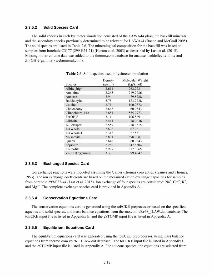
2.3.5.2 Solid Species Card
The solid species in each lysimeter simulation consisted of the LAWA44 glass, the backfill minerals, and the secondary species previously determined to be relevant for LAWA44 (Bacon and McGrail 2005). The solid species are listed in Table 2.6. The mineralogical composition for the backfill was based on samples from borehole C3177 (299-E24-21) (Horton et al. 2003) as described by Last et al. (2015). Missing molar volume data was added to the thermo.com database for anatase, baddelleyite, illite and Zn(OH)2(gamma) (webmineral.com).
Table 2.6. Solid species used in lysimeter simulation
Species Density (g/cm3)
Molecular Weight (kg/kmol)
Albite_high 2.611 262.223 Analcime 2.265 219.2786 Anatase 3.9 79.8788 Baddeleyite 5.75 123.2228 Calcite 2.71 100.0872 Chalcedony 2.648 60.0843 Clinochlore-14A 2.684 555.7973 Fe(OH)3 3.11 106.869 Gibbsite 2.441 78.0036 K-Feldspar 2.557 278.3315 LAWA44 2.698 67.06 LAWA44-H 2.315 57.55 Muscovite 2.831 398.3081 Quartz 2.648 60.0843 Sepiolite 2.268 647.8304 Tremolite 2.977 812.3665 Zn(OH)2(gamma) 3.33 99.4047
2.3.5.3 Exchanged Species Card
Ion exchange reactions were modeled assuming the Gaines-Thomas convention (Gaines and Thomas, 1953). The ion exchange coefficients are based on the measured cation exchange capacities for samples from borehole 299-E33-44 (Last et al. 2015). Ion exchange of four species are considered: Na+, Ca2+, K+, and Mg2+. The complete exchange species card is provided in Appendix A.
2.3.5.4 Conservation Equations Card
The conservation equations card is generated using the toECKE preprocessor based on the specified aqueous and solid species, and mass balance equations from thermo.com.v8.r6+_ILAW.dat database. The toECKE input file is listed in Appendix E, and the eSTOMP input file is listed in Appendix A.
2.3.5.5 Equilibrium Equations Card
The equilibrium equations card was generated using the toECKE preprocessor, using mass balance equations from thermo.com.v8.r6+_ILAW.dat database. The toECKE input file is listed in Appendix E, and the eSTOMP input file is listed in Appendix A. For aqueous species, the equations are selected from
2.13
the thermo.com.v8.r6+_ILAW.dat database. For ion exchange species, the relevant mass balance equations were taken from the llnl.dat database, distributed with PHREEQC (Parkhurst and Appello 1999) and added to the thermo.com.v8.r6+_ILAW.dat database.
2.3.5.6 Equilibrium Reactions Card
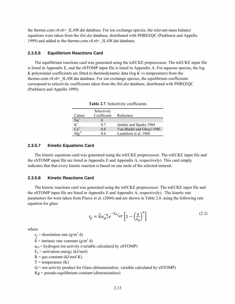
The equilibrium reactions card was generated using the toECKE preprocessor. The toECKE input file is listed in Appendix E, and the eSTOMP input file is listed in Appendix A. For aqueous species, the log K polynomial coefficients are fitted to thermodynamic data (log K vs temperature) from the thermo.com.v8.r6+_ILAW.dat database. For ion exchange species, the equilibrium coefficients correspond to selectivity coefficients taken from the llnl.dat database, distributed with PHREEQC (Parkhurst and Appello 1999).
Table 2.7. Selectivity coefficients
Cation Selectivity Coefficient Reference
Na+ 0 K+ 0.7 Jardine and Sparks 1984 Ca2+ 0.8 Van Bladel and Gheyi 1980 Mg2+ 0.6 Laudelout et al. 1968
2.3.5.7 Kinetic Equations Card
The kinetic equations card was generated using the toECKE preprocessor. The toECKE input file and the eSTOMP input file are listed in Appendix E and Appendix A, respectively). This card simply indicates that that every kinetic reaction is based on one mole of the selected mineral.
2.3.5.8 Kinetic Reactions Card
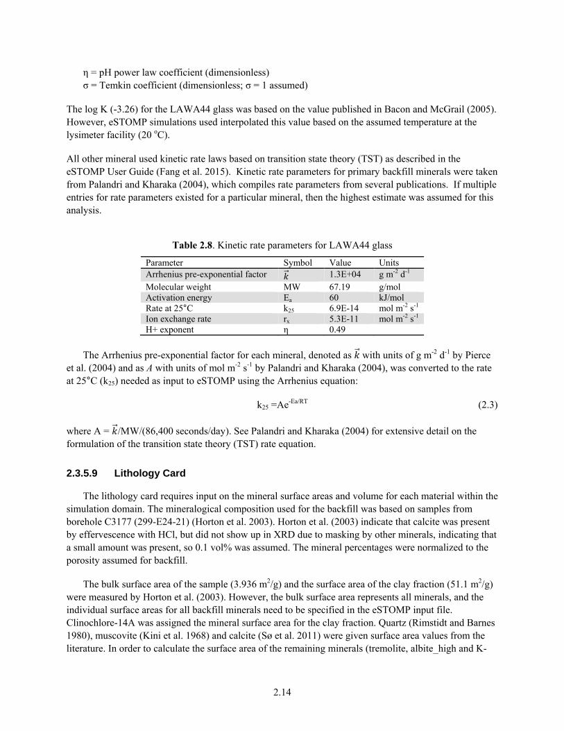
The kinetic reactions card was generated using the toECKE preprocessor. The toECKE input file and the eSTOMP input file are listed in Appendix E and Appendix A, respectively). The kinetic rate parameters for were taken from Pierce et al. (2004) and are shown in Table 2.8. using the following rate equation for glass
1 (2.2)
where rg = dissolution rate (g/m2 d)
= intrinsic rate constant (g/m2 d) aH+= hydrogen ion activity (variable calculated by eSTOMP) Ea = activation energy (kJ/mol) R = gas constant (kJ/mol K) T = temperature (K) Q = ion activity product for Glass (dimensionless; variable calculated by eSTOMP) Kg = pseudo-equilibrium constant (dimensionless)
2.14
η = pH power law coefficient (dimensionless) σ = Temkin coefficient (dimensionless; σ = 1 assumed)
The log K (-3.26) for the LAWA44 glass was based on the value published in Bacon and McGrail (2005). However, eSTOMP simulations used interpolated this value based on the assumed temperature at the lysimeter facility (20 oC).
All other mineral used kinetic rate laws based on transition state theory (TST) as described in the eSTOMP User Guide (Fang et al. 2015). Kinetic rate parameters for primary backfill minerals were taken from Palandri and Kharaka (2004), which compiles rate parameters from several publications. If multiple entries for rate parameters existed for a particular mineral, then the highest estimate was assumed for this analysis.
Table 2.8. Kinetic rate parameters for LAWA44 glass
Parameter Symbol Value Units Arrhenius pre-exponential factor 1.3E+04 g m-2 d-1 Molecular weight MW 67.19 g/mol Activation energy Ea 60 kJ/mol Rate at 25°C k25 6.9E-14 mol m-2 s-1 Ion exchange rate rx 5.3E-11 mol m-2 s-1 H+ exponent η 0.49
The Arrhenius pre-exponential factor for each mineral, denoted as with units of g m-2 d-1 by Pierce et al. (2004) and as A with units of mol m-2 s-1 by Palandri and Kharaka (2004), was converted to the rate at 25°C (k25) needed as input to eSTOMP using the Arrhenius equation:
k25 =Ae-Ea/RT (2.3)
where A = /MW/(86,400 seconds/day). See Palandri and Kharaka (2004) for extensive detail on the formulation of the transition state theory (TST) rate equation.
2.3.5.9 Lithology Card
The lithology card requires input on the mineral surface areas and volume for each material within the simulation domain. The mineralogical composition used for the backfill was based on samples from borehole C3177 (299-E24-21) (Horton et al. 2003). Horton et al. (2003) indicate that calcite was present by effervescence with HCl, but did not show up in XRD due to masking by other minerals, indicating that a small amount was present, so 0.1 vol% was assumed. The mineral percentages were normalized to the porosity assumed for backfill.
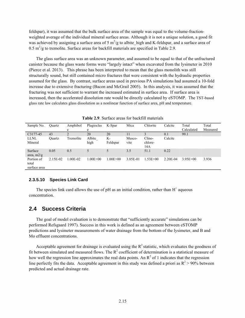
The bulk surface area of the sample (3.936 m2/g) and the surface area of the clay fraction (51.1 m2/g) were measured by Horton et al. (2003). However, the bulk surface area represents all minerals, and the individual surface areas for all backfill minerals need to be specified in the eSTOMP input file. Clinochlore-14A was assigned the mineral surface area for the clay fraction. Quartz (Rimstidt and Barnes 1980), muscovite (Kini et al. 1968) and calcite (Sø et al. 2011) were given surface area values from the literature. In order to calculate the surface area of the remaining minerals (tremolite, albite_high and K-
2.15
feldspar), it was assumed that the bulk surface area of the sample was equal to the volume-fraction-weighted average of the individual mineral surface areas. Although it is not a unique solution, a good fit was achieved by assigning a surface area of 5 m2/g to albite_high and K-feldspar, and a surface area of 0.5 m2/g to tremolite. Surface areas for backfill materials are specified in Table 2.9.
The glass surface area was an unknown parameter, and assumed to be equal to that of the unfractured canister because the glass waste forms were “largely intact” when excavated from the lysimeter in 2010 (Pierce et al. 2013). This phrase has been interpreted to mean that the glass monolith was still structurally sound, but still contained micro fractures that were consistent with the hydraulic properties assumed for the glass. By contrast, surface areas used in previous PA simulations had assumed a 10-fold increase due to extensive fracturing (Bacon and McGrail 2005). In this analysis, it was assumed that the fracturing was not sufficient to warrant the increased estimated in surface area. If surface area is increased, then the accelerated dissolution rate would be directly calculated by eSTOMP. The TST-based glass rate law calculates glass dissolution as a nonlinear function of surface area, pH and temperature.
Table 2.9. Surface areas for backfill materials
Sample No. Quartz Amphibole
Plagioclase
K-Spar Mica Chlorite Calcite Total Calculated
Total Measured
C3177-45 43 2 20 20 11 3 0.1 99.1 LLNL Mineral
Quartz Tremolite Albite_ high
K-Feldspar
Musco-vite
Clino-chlore-14A
Calcite
Surface area, m2/g
0.05 0.5 5 5 3.5 51.1 0.22
Portion of total surface area
2.15E-02 1.00E-02 1.00E+00 1.00E+00 3.85E-01 1.53E+00 2.20E-04 3.95E+00 3.936
2.3.5.10 Species Link Card
The species link card allows the use of pH as an initial condition, rather than H+ aqueous concentration.
2.4 Success Criteria
The goal of model evaluation is to demonstrate that “sufficiently accurate” simulations can be performed Refsgaard 1997). Success in this work is defined as an agreement between eSTOMP predictions and lysimeter measurements of water drainage from the bottom of the lysimeter, and B and Mo effluent concentrations.
Acceptable agreement for drainage is evaluated using the R2 statistic, which evaluates the goodness of fit between simulated and measured flows. The R2 coefficient of determination is a statistical measure of how well the regression line approximates the real data points. An R2 of 1 indicates that the regression line perfectly fits the data. Acceptable agreement in this study was defined a priori as R2 > 90% between predicted and actual drainage rate.
2.16
Because fewer data exist for the B and Mo pore-water concentrations, the evaluation is based on the observed B and Mo effluent concentrations fitting within a range of minimum and maximum predicted B and Mo effluent concentrations.
2.5 Simulation Results
One simulation was executed with a recharge rate of 0.00373 cm/day. The slope of the modeled drainage compares well to the slope of the line fitted to the measured drainage, which has an R2 of 0.934, indicating that the rates are the same (Figure 2.6). The initial water saturation was assumed to be 0.15, so slight differences in the slope of the modeled drainage are due to this assumption. The two curves are offset because modeled drainage begins earlier. The observed drainage is periodic due to periodic irrigation of the lysimeters, and the slope of the fitted line reflects the average recharge over time. Although the modeled drainage begins earlier, the slopes of the lines are nearly the same, indicating that the average recharge rate over time is the same. Performance assessment simulations will also assume a constant recharge rate.
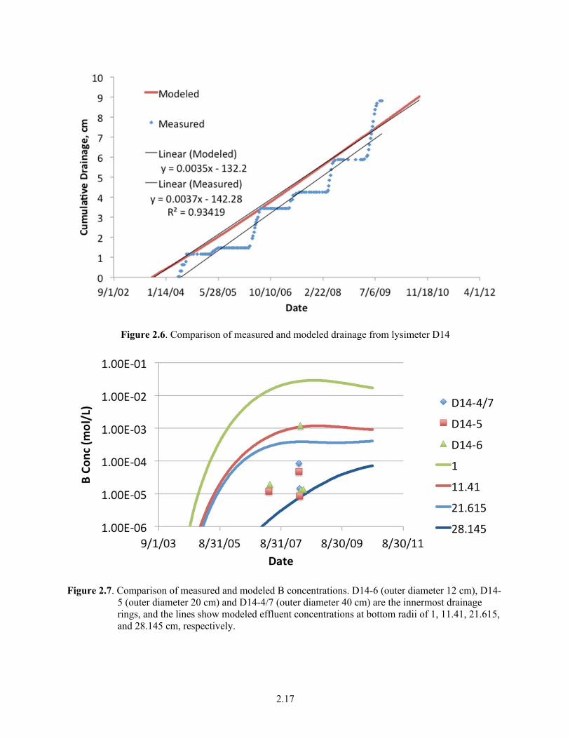
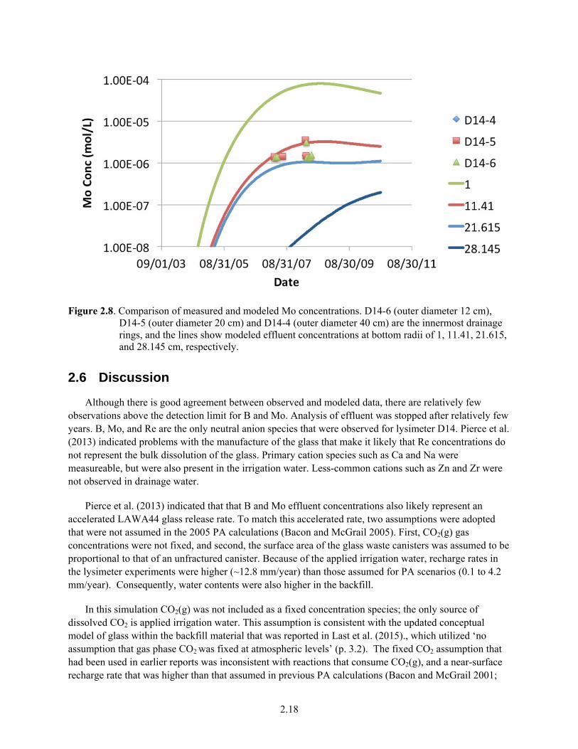
Relatively few concentration data were available for comparison for both B and Mo as several samples were noted as non-detectable concentrations. These non-detects were not used in this analysis for comparison. The non-detection level for B was 7.6 × 10-6.mol/L. The non-detect level for Mo was not reported.
The simulated and measured effluent concentrations for B and Mo are presented in Figure 2.7 and Figure 2.8, respectively. Both figures plot continuous lines as the modeled effluent, and points for the measured effluent. Colors are used to show the position of the measured and simulated effluents within the lysimeter. For example, D14-6 (in green) represents the outer diameter of 12 cm, D14-5 (in red) represents the outer diameter of 20 cm, and D14-4/7 (in blue) represents the outer diameter of 40 cm. These diameters represent the innermost drainage rings as described in Meyer (2001). The lines corresponding to these colors represent the simulated effluent concentrations at the bottom of the simulator at radii of 1, 11.41, 21.615, and 28.145 cm, respectively, which correspond to the bounds of the rings within the simulator. Because these represent bounds, there is an additional radius at 1 cm (a different shade of blue).
Results show that the observed effluent B concentrations fall within the range of the modeled concentrations. (Figure 2.8). Similarly, observed effluent Mo concentrations are also within the range of modeled effluent Mo concentrations (Figure 2.8). In general, the range in simulated concentrations is greater than range in concentrations measured in the field. For example, B concentrations are consistently overpredicted. However, the observed concentrations do fall within the predicted concentrations at the boundaries of the three innermost drainage rings. Lower concentrations may also have been below the detection limits for B (7.6x10⁻⁶ mol/l) and Mo (not reported), which cannot be used for comparison in this study. Given uncertainties related to heterogeneities in lysimeter sediments, reactive surface areas and phase-separated glass, the extent of model evaluation is limited, and bounding concentration estimates are reasonable metrics in this analysis.
2.17
Figure 2.6. Comparison of measured and modeled drainage from lysimeter D14
Figure 2.7. Comparison of measured and modeled B concentrations. D14-6 (outer diameter 12 cm), D14-5 (outer diameter 20 cm) and D14-4/7 (outer diameter 40 cm) are the innermost drainage rings, and the lines show modeled effluent concentrations at bottom radii of 1, 11.41, 21.615, and 28.145 cm, respectively.
2.18
Figure 2.8. Comparison of measured and modeled Mo concentrations. D14-6 (outer diameter 12 cm), D14-5 (outer diameter 20 cm) and D14-4 (outer diameter 40 cm) are the innermost drainage rings, and the lines show modeled effluent concentrations at bottom radii of 1, 11.41, 21.615, and 28.145 cm, respectively.
2.6 Discussion
Although there is good agreement between observed and modeled data, there are relatively few observations above the detection limit for B and Mo. Analysis of effluent was stopped after relatively few years. B, Mo, and Re are the only neutral anion species that were observed for lysimeter D14. Pierce et al. (2013) indicated problems with the manufacture of the glass that make it likely that Re concentrations do not represent the bulk dissolution of the glass. Primary cation species such as Ca and Na were measureable, but were also present in the irrigation water. Less-common cations such as Zn and Zr were not observed in drainage water.
Pierce et al. (2013) indicated that that B and Mo effluent concentrations also likely represent an accelerated LAWA44 glass release rate. To match this accelerated rate, two assumptions were adopted that were not assumed in the 2005 PA calculations (Bacon and McGrail 2005). First, CO2(g) gas concentrations were not fixed, and second, the surface area of the glass waste canisters was assumed to be proportional to that of an unfractured canister. Because of the applied irrigation water, recharge rates in the lysimeter experiments were higher (~12.8 mm/year) than those assumed for PA scenarios (0.1 to 4.2 mm/year). Consequently, water contents were also higher in the backfill.
In this simulation CO2(g) was not included as a fixed concentration species; the only source of dissolved CO2 is applied irrigation water. This assumption is consistent with the updated conceptual model of glass within the backfill material that was reported in Last et al. (2015)., which utilized ‘no assumption that gas phase CO2 was fixed at atmospheric levels’ (p. 3.2). The fixed CO2 assumption that had been used in earlier reports was inconsistent with reactions that consume CO2(g), and a near-surface recharge rate that was higher than that assumed in previous PA calculations (Bacon and McGrail 2001;
2.19
2005). Not fixing the CO2 gas concentration allowed the pH in the glass to increase, thereby increasing the dissolution rate. CO2 gas concentrations in the vadose zone are a balance between sources/sinks of CO2 gas and gas-phase diffusion/advection. The true CO2 gas partial pressures are likely to lie between those calculated by a fixed assumption and non-fixed assumption.
The glass corrosion rate is proportional to the surface area of the glass. The surface area of the glass was assumed to be equal to the surface area of the glass canister. In contrast to the PA simulations where the surface area of the glass was assumed to increase 10-fold over the surface area of the canister, no increase in surface area was assumed due to fracturing. Increasing the surface area 10-fold would increase the release of tracer species at least 10-fold, and likely more due to the nonlinear effect of increasing pH.
Because of uncertainties related to the manufacture of the glass, which may have caused accelerated release of B and Mo, it is not possible to confirm whether the assumptions regarding fixed CO2(g) or surface area are valid with regards to glass that will be produced by the Hanford Tank Waste Treatment and Immobilization Plant (WTP). It can only be confirmed that using these assumptions caused the modeled results to match the observations for the glass used in these experiments.
There are a number of uncertainties in the experimental data collected that cannot be resolved. The formation of iron rich alloys may have accelerated the release of B and Mo. It is not known how the water content in the backfill varied with time. It is not known how the gas phase CO2 varied with time. It is not known how the fracture surface area of the glass varied with time. The absence of these sensitive data make it difficult to obtain a unique solution and use this experiment for validation.
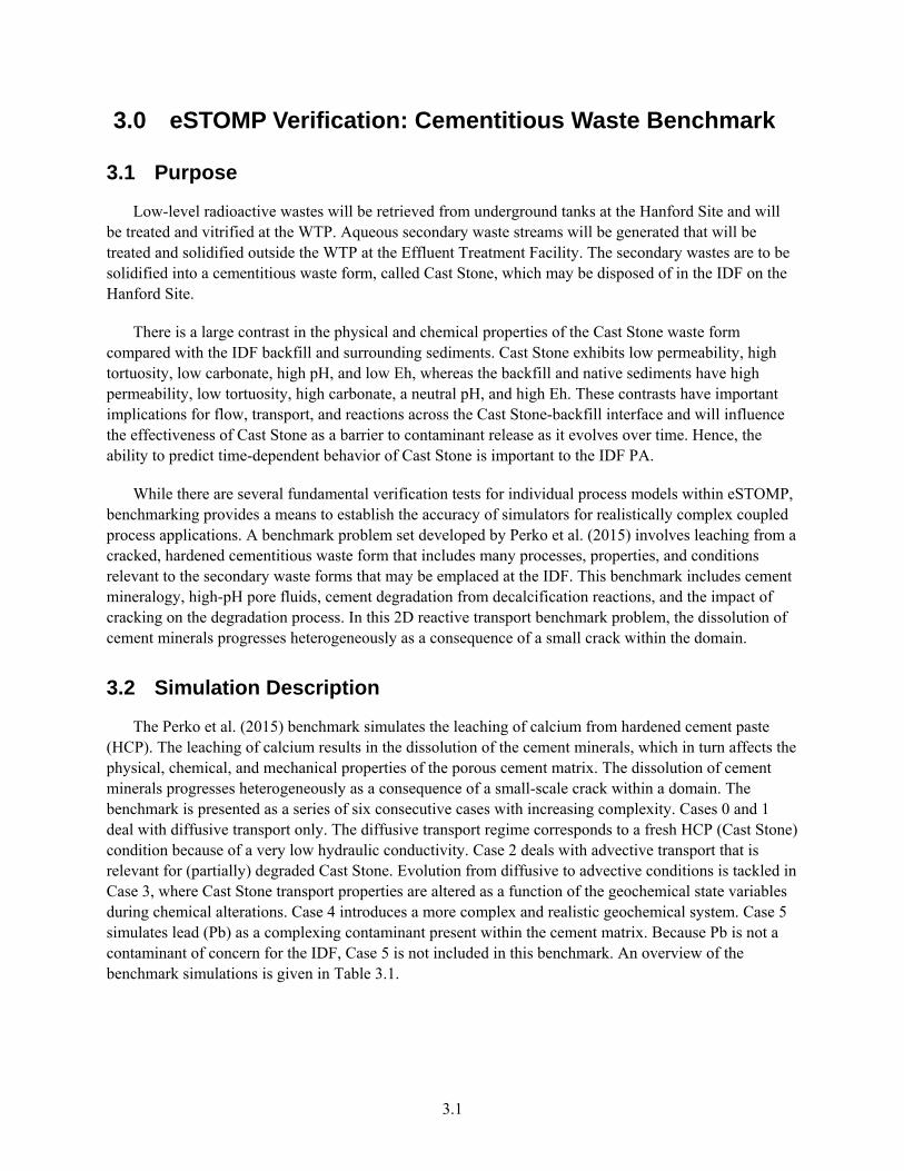
3.1
3.0 eSTOMP Verification: Cementitious Waste Benchmark
3.1 Purpose
Low-level radioactive wastes will be retrieved from underground tanks at the Hanford Site and will be treated and vitrified at the WTP. Aqueous secondary waste streams will be generated that will be treated and solidified outside the WTP at the Effluent Treatment Facility. The secondary wastes are to be solidified into a cementitious waste form, called Cast Stone, which may be disposed of in the IDF on the Hanford Site.
There is a large contrast in the physical and chemical properties of the Cast Stone waste form compared with the IDF backfill and surrounding sediments. Cast Stone exhibits low permeability, high tortuosity, low carbonate, high pH, and low Eh, whereas the backfill and native sediments have high permeability, low tortuosity, high carbonate, a neutral pH, and high Eh. These contrasts have important implications for flow, transport, and reactions across the Cast Stone-backfill interface and will influence the effectiveness of Cast Stone as a barrier to contaminant release as it evolves over time. Hence, the ability to predict time-dependent behavior of Cast Stone is important to the IDF PA.
While there are several fundamental verification tests for individual process models within eSTOMP, benchmarking provides a means to establish the accuracy of simulators for realistically complex coupled process applications. A benchmark problem set developed by Perko et al. (2015) involves leaching from a cracked, hardened cementitious waste form that includes many processes, properties, and conditions relevant to the secondary waste forms that may be emplaced at the IDF. This benchmark includes cement mineralogy, high-pH pore fluids, cement degradation from decalcification reactions, and the impact of cracking on the degradation process. In this 2D reactive transport benchmark problem, the dissolution of cement minerals progresses heterogeneously as a consequence of a small crack within the domain.
3.2 Simulation Description
The Perko et al. (2015) benchmark simulates the leaching of calcium from hardened cement paste (HCP). The leaching of calcium results in the dissolution of the cement minerals, which in turn affects the physical, chemical, and mechanical properties of the porous cement matrix. The dissolution of cement minerals progresses heterogeneously as a consequence of a small-scale crack within a domain. The benchmark is presented as a series of six consecutive cases with increasing complexity. Cases 0 and 1 deal with diffusive transport only. The diffusive transport regime corresponds to a fresh HCP (Cast Stone) condition because of a very low hydraulic conductivity. Case 2 deals with advective transport that is relevant for (partially) degraded Cast Stone. Evolution from diffusive to advective conditions is tackled in Case 3, where Cast Stone transport properties are altered as a function of the geochemical state variables during chemical alterations. Case 4 introduces a more complex and realistic geochemical system. Case 5 simulates lead (Pb) as a complexing contaminant present within the cement matrix. Because Pb is not a contaminant of concern for the IDF, Case 5 is not included in this benchmark. An overview of the benchmark simulations is given in Table 3.1.
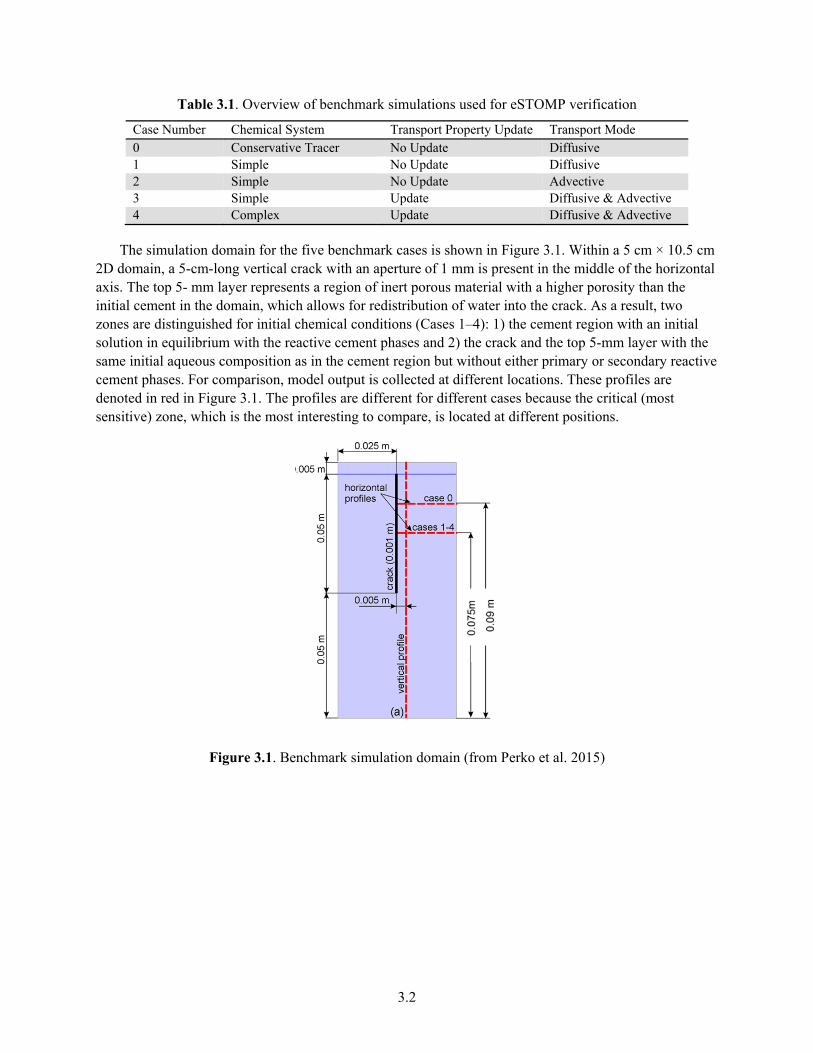
3.2
Table 3.1. Overview of benchmark simulations used for eSTOMP verification
Case Number Chemical System Transport Property Update Transport Mode 0 Conservative Tracer No Update Diffusive 1 Simple No Update Diffusive 2 Simple No Update Advective 3 Simple Update Diffusive & Advective4 Complex Update Diffusive & Advective
The simulation domain for the five benchmark cases is shown in Figure 3.1. Within a 5 cm × 10.5 cm 2D domain, a 5-cm-long vertical crack with an aperture of 1 mm is present in the middle of the horizontal axis. The top 5- mm layer represents a region of inert porous material with a higher porosity than the initial cement in the domain, which allows for redistribution of water into the crack. As a result, two zones are distinguished for initial chemical conditions (Cases 1–4): 1) the cement region with an initial solution in equilibrium with the reactive cement phases and 2) the crack and the top 5-mm layer with the same initial aqueous composition as in the cement region but without either primary or secondary reactive cement phases. For comparison, model output is collected at different locations. These profiles are denoted in red in Figure 3.1. The profiles are different for different cases because the critical (most sensitive) zone, which is the most interesting to compare, is located at different positions.
Figure 3.1. Benchmark simulation domain (from Perko et al. 2015)
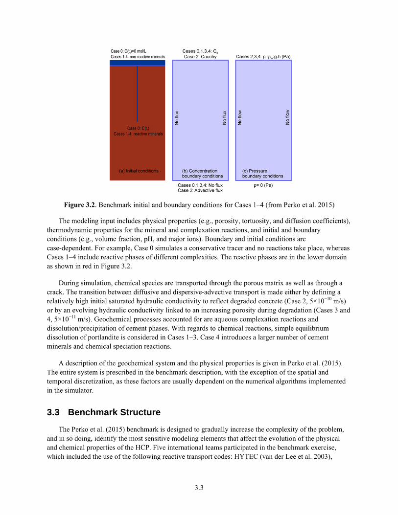
3.3
Figure 3.2. Benchmark initial and boundary conditions for Cases 1–4 (from Perko et al. 2015)
The modeling input includes physical properties (e.g., porosity, tortuosity, and diffusion coefficients), thermodynamic properties for the mineral and complexation reactions, and initial and boundary conditions (e.g., volume fraction, pH, and major ions). Boundary and initial conditions are case-dependent. For example, Case 0 simulates a conservative tracer and no reactions take place, whereas Cases 1–4 include reactive phases of different complexities. The reactive phases are in the lower domain as shown in red in Figure 3.2.
During simulation, chemical species are transported through the porous matrix as well as through a crack. The transition between diffusive and dispersive-advective transport is made either by defining a relatively high initial saturated hydraulic conductivity to reflect degraded concrete (Case 2, 5×10⁻¹⁰ m/s) or by an evolving hydraulic conductivity linked to an increasing porosity during degradation (Cases 3 and 4, 5×10⁻¹¹ m/s). Geochemical processes accounted for are aqueous complexation reactions and dissolution/precipitation of cement phases. With regards to chemical reactions, simple equilibrium dissolution of portlandite is considered in Cases 1–3. Case 4 introduces a larger number of cement minerals and chemical speciation reactions.
A description of the geochemical system and the physical properties is given in Perko et al. (2015). The entire system is prescribed in the benchmark description, with the exception of the spatial and temporal discretization, as these factors are usually dependent on the numerical algorithms implemented in the simulator.
3.3 Benchmark Structure
The Perko et al. (2015) benchmark is designed to gradually increase the complexity of the problem, and in so doing, identify the most sensitive modeling elements that affect the evolution of the physical and chemical properties of the HCP. Five international teams participated in the benchmark exercise, which included the use of the following reactive transport codes: HYTEC (van der Lee et al. 2003),
3.4
MIN3P (Mayer et al. 2002), OGS-GEM (Kulik et al. 2013), ORCHESTRA (Meeussen 2003), and COMSOL Multiphysics-iPHREEQC, referenced as SC3K (Parkhurst et al. 1999; COMSOL 2008). Not all codes reported results for every benchmark simulation, either due to code limitations or to disparate simulation results. For example, ORCHESTRA only participated in Case 1, whereas MIN3P and SC3K participated in all of the benchmark cases. The small scale of the benchmark simulations (5 cm × 10.5 cm 2D domain) means that comparisons of results were also performed at a very small scale, and that such differences at the field-scale may be less significant. The published benchmarks were verified based on yielding similar patterns in concentrations and mineralogy. In addition, the benchmark participants determined that differences in results also depended on 1) the weighting and conservation properties of different numerical methods, 2) the coupling between transport and reactive solver, and 3) the agreement of thermodynamic database (Perko et al. 2015).
3.4 Solution Methods
There are two major approaches to coupling hydrological transport and geochemical reactions: 1) the one-step or global implicit method (GIM) and 2) the operator split method (OSM) (Steefel and MacQuarrie 1996). The first approach solves the set of transport and chemical reaction equations simultaneously. All of the interaction chemistry is inserted directly into the transport equations, thereby reducing the problem to one strongly non-linear equation set. Because of the excessive requirement of computer resources, GIM is often not practical for large two- and three-dimensional applications. Yeh and Tripathi (1989) have found that the second method, OSM, can be a more practical approach. This approach is called operator split because it solves the advection-dispersion and reaction operations sequentially, in two separate steps. The geochemistry equations are typically solved first, followed by a transport step. Because these steps are decoupled, numerical errors can occur. If an iterative approach is used, then the “splitting error” can be reduced. The iteration would proceed until the concentration computed in the reaction equation agrees with the concentration computed in the transport equation within a certain tolerance. However, Yeh and Tripathi (1989) point out that several iterations are often required within a single time step. If the equations are highly non-linear, the iterative solution may not converge (Steefel and MacQuarrie 1996).
Although GIM can suffer from a lack of computational efficiency, the global convergence properties may be better than the multi-step methods. With a fully coupled scheme, it is sometimes possible to take larger time steps. This is often the case when the governing differential equations are “stiff”; that is, the time step needed to maintain numerical stability is much smaller than the time step needed for an accurate solution. This stiffness is common among systems that contain processes occurring over vastly different time scales, such as in equilibrium (fast) vs. kinetic (slow) chemical reactions.
3.4.1 Numerical Methods
Numerical approaches differed for the simulators participating in the benchmark study, with different transport models and solution methods, geochemical solvers, and coupling algorithms (iterative and non-iterative). Some of the codes used a finite volume method (FVM), whereas other used a finite element method (FEM) for the solution of the partial differential equations. The unknowns for FVM and FEM are at the cell center and vertex, respectively. For example, the MIN3P code is based on the FVM and uses GIM for solving the geochemistry and transport equations. HYTEC is based on an FVM with representative elementary volumes for mass transport and an iterative OSM for coupling between
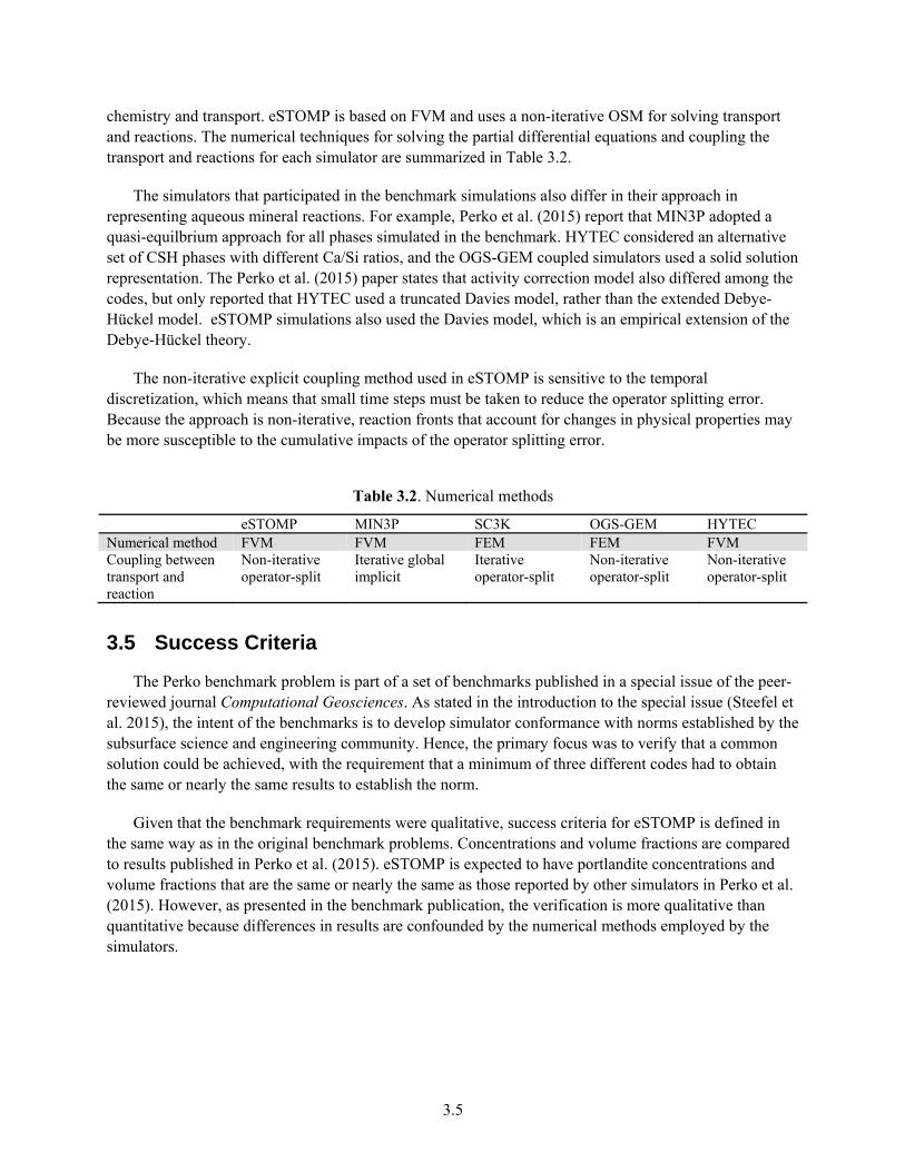
3.5
chemistry and transport. eSTOMP is based on FVM and uses a non-iterative OSM for solving transport and reactions. The numerical techniques for solving the partial differential equations and coupling the transport and reactions for each simulator are summarized in Table 3.2.
The simulators that participated in the benchmark simulations also differ in their approach in representing aqueous mineral reactions. For example, Perko et al. (2015) report that MIN3P adopted a quasi-equilbrium approach for all phases simulated in the benchmark. HYTEC considered an alternative set of CSH phases with different Ca/Si ratios, and the OGS-GEM coupled simulators used a solid solution representation. The Perko et al. (2015) paper states that activity correction model also differed among the codes, but only reported that HYTEC used a truncated Davies model, rather than the extended Debye-Hückel model. eSTOMP simulations also used the Davies model, which is an empirical extension of the Debye-Hückel theory.
The non-iterative explicit coupling method used in eSTOMP is sensitive to the temporal discretization, which means that small time steps must be taken to reduce the operator splitting error. Because the approach is non-iterative, reaction fronts that account for changes in physical properties may be more susceptible to the cumulative impacts of the operator splitting error.
Table 3.2. Numerical methods
eSTOMP MIN3P SC3K OGS-GEM HYTEC Numerical method FVM FVM FEM FEM FVM Coupling between transport and reaction
Non-iterative operator-split
Iterative global implicit
Iterative operator-split
Non-iterative operator-split
Non-iterative operator-split
3.5 Success Criteria
The Perko benchmark problem is part of a set of benchmarks published in a special issue of the peer-reviewed journal Computational Geosciences. As stated in the introduction to the special issue (Steefel et al. 2015), the intent of the benchmarks is to develop simulator conformance with norms established by the subsurface science and engineering community. Hence, the primary focus was to verify that a common solution could be achieved, with the requirement that a minimum of three different codes had to obtain the same or nearly the same results to establish the norm.
Given that the benchmark requirements were qualitative, success criteria for eSTOMP is defined in the same way as in the original benchmark problems. Concentrations and volume fractions are compared to results published in Perko et al. (2015). eSTOMP is expected to have portlandite concentrations and volume fractions that are the same or nearly the same as those reported by other simulators in Perko et al. (2015). However, as presented in the benchmark publication, the verification is more qualitative than quantitative because differences in results are confounded by the numerical methods employed by the simulators.
3.6
3.6 Simulation Input File Description
Simulation case names (Case 0 through Case 4) follow those in Perko et al. (2015). For each case, a flow simulation was executed to obtain a steady-state flow field, which served as an initial condition for the transient simulations. Results from the transient simulations are compared as part of the benchmark.
The sources of data for the eSTOMP input files are given in the sections below, with each card described in a separate section. These cards organize inputs and describe the individual sections of the input file. Model input parameters are from Perko et al. (2015) unless otherwise noted. The complete eSTOMP input files for each case are provided in Appendix F through Appendix J.
3.6.1 Solution Control Card
The solution control card controls general operational aspects of a simulation. Keywords are used to indicate solute or reactive transport, and solution options.
If porosity will be updated, the keyword “porosity” is needed so that as the cementitious waste form undergoes dissolution, and secondary minerals precipitate and dissolve, new mineral volumes are used to calculate changes in porosity for the porous medium. This option also includes an inert volume fraction that was used in the Perko et al. (2015) benchmarks also involve an inert volume fraction.
3.6.2 Grid Card
As previously stated, the spatial discretization used by the other simulators in the Perko et al. (2015) benchmark is not described, since the grid discretization is usually dependent on the numerical algorithms implemented in the simulator. Hence, the model grid was modified to fit the benchmark, and was mostly dependent on numerical considerations.
The model grid is based on the schematics shown in Figure 3.1 and Figure 3.2. The grid was constructed to define boundary of cement, crack, and the top inactive zones, as well as the location of the cross sections for model comparisons. Cases 0 to 2 use a refined grid and use the principle of symmetry to model half of the domain (minimum spacing = 0.125 mm, maximum spacing = 1.5 mm). In Cases 3 and 4, the full domain is used, but a coarser discretization is used to reduce the simulation time (minimum spacing = 1 mm, maximum spacing = 2.5 mm ).
3.6.3 Rock/Soil Zonation Card
The benchmark computational domain was subdivided into three distinct geologic units: top layer, cement, and crack, which were specified under the rock/soil zonation card. Once defined, physical and chemical properties were associated with each unit, as described in the cards below.
3.6.4 Mechanical Properties Card
The mechanical properties card allows the user to assign values to the particle density, porosity, specific storativity, compressibility, and tortuosity functions for each defined rock/soil type. The parameters used in each of the case studies are described in Table 3.3 for the three material types: top
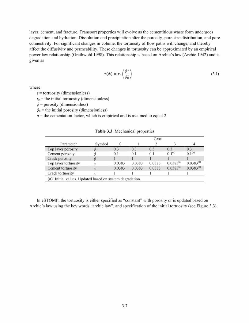
3.7
layer, cement, and fracture. Transport properties will evolve as the cementitious waste form undergoes degradation and hydration. Dissolution and precipitation alter the porosity, pore size distribution, and pore connectivity. For significant changes in volume, the tortuosity of flow paths will change, and thereby affect the diffusivity and permeability. These changes in tortuosity can be approximated by an empirical power law relationship (Grathwohl 1998). This relationship is based on Archie’s law (Archie 1942) and is given as
(3.1)
where τ = tortuosity (dimensionless) τ0 = the initial tortuosity (dimensionless) ϕ = porosity (dimensionless) ϕ0 = the initial porosity (dimensionless) a = the cementation factor, which is empirical and is assumed to equal 2
Table 3.3. Mechanical properties
Parameter Symbol Case
0 1 2 3 4 Top layer porosity ϕ 0.3 0.3 0.3 0.3 0.3 Cement porosity ϕ 0.1 0.1 0.1 0.1(a) 0.1(a)
Crack porosity ϕ 1 1 1 1 1 Top layer tortuosity 0.0383 0.0383 0.0383 0.0383(a) 0.0383(a)
Cement tortuosity 0.0383 0.0383 0.0383 0.0383(a) 0.0383(a) Crack tortuosity 1 1 1 1 1
(a) Initial values. Updated based on system degradation.
In eSTOMP, the tortuosity is either specified as “constant” with porosity or is updated based on Archie’s law using the key words “archie law”, and specification of the initial tortuosity (see Figure 3.3).
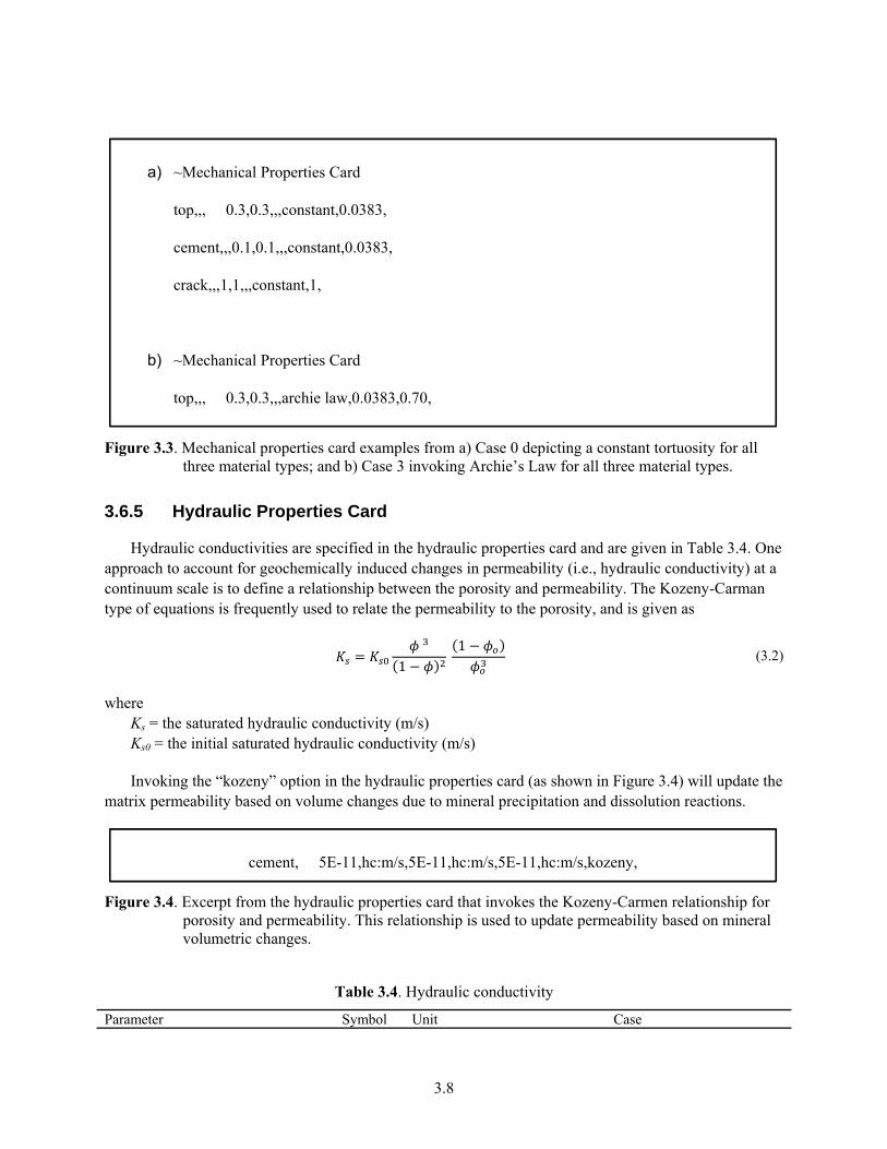
3.8
Figure 3.3. Mechanical properties card examples from a) Case 0 depicting a constant tortuosity for all three material types; and b) Case 3 invoking Archie’s Law for all three material types.
3.6.5 Hydraulic Properties Card
Hydraulic conductivities are specified in the hydraulic properties card and are given in Table 3.4. One approach to account for geochemically induced changes in permeability (i.e., hydraulic conductivity) at a continuum scale is to define a relationship between the porosity and permeability. The Kozeny-Carman type of equations is frequently used to relate the permeability to the porosity, and is given as
11
(3.2)
where Ks = the saturated hydraulic conductivity (m/s) Ks0 = the initial saturated hydraulic conductivity (m/s)
Invoking the “kozeny” option in the hydraulic properties card (as shown in Figure 3.4) will update the matrix permeability based on volume changes due to mineral precipitation and dissolution reactions.
Figure 3.4. Excerpt from the hydraulic properties card that invokes the Kozeny-Carmen relationship for porosity and permeability. This relationship is used to update permeability based on mineral volumetric changes.
Table 3.4. Hydraulic conductivity
Parameter Symbol Unit Case
a) ~Mechanical Properties Card
top,,, 0.3,0.3,,,constant,0.0383,
cement,,,0.1,0.1,,,constant,0.0383,
crack,,,1,1,,,constant,1,
b) ~Mechanical Properties Card
top,,, 0.3,0.3,,,archie law,0.0383,0.70,
cement, 5E-11,hc:m/s,5E-11,hc:m/s,5E-11,hc:m/s,kozeny,
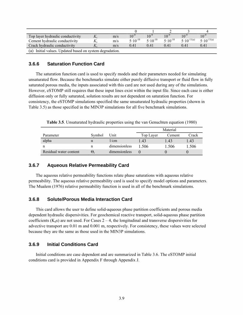
3.9
0 1 2 3 4 Top layer hydraulic conductivity Ks m/s 10-9 10-9 10-9 10-9 10-9 Cement hydraulic conductivity Ks m/s 5·10-10 5·10-10 5·10-10 5·10-11(a) 5·10-11(a) Crack hydraulic conductivity Ks m/s 0.41 0.41 0.41 0.41 0.41 (a) Initial values. Updated based on system degradation.
3.6.6 Saturation Function Card
The saturation function card is used to specify models and their parameters needed for simulating unsaturated flow. Because the benchmarks simulate either purely diffusive transport or fluid flow in fully saturated porous media, the inputs associated with this card are not used during any of the simulations. However, eSTOMP still requires that these input lines exist within the input file. Since each case is either diffusion only or fully saturated, solution results are not dependent on saturation function. For consistency, the eSTOMP simulations specified the same unsaturated hydraulic properties (shown in Table 3.5) as those specified in the MIN3P simulations for all five benchmark simulations.
Table 3.5. Unsaturated hydraulic properties using the van Genuchten equation (1980)
Parameter Symbol Unit Material
Top Layer Cement Crackalpha α 1/cm 1.43 1.43 1.43 n n dimensionless 1.506 1.506 1.506 Residual water content Θr dimensionless 0 0 0
3.6.7 Aqueous Relative Permeability Card
The aqueous relative permeability functions relate phase saturations with aqueous relative permeability. The aqueous relative permeability card is used to specify model options and parameters. The Mualem (1976) relative permeability function is used in all of the benchmark simulations.
3.6.8 Solute/Porous Media Interaction Card
This card allows the user to define solid-aqueous phase partition coefficients and porous media dependent hydraulic dispersivities. For geochemical reactive transport, solid-aqueous phase partition coefficients (Kds) are not used. For Cases 2 – 4, the longitudinal and transverse dispersivities for advective transport are 0.01 m and 0.001 m, respectively. For consistency, these values were selected because they are the same as those used in the MIN3P simulations.
3.6.9 Initial Conditions Card
Initial conditions are case dependent and are summarized in Table 3.6. The eSTOMP initial conditions card is provided in Appendix F through Appendix J.
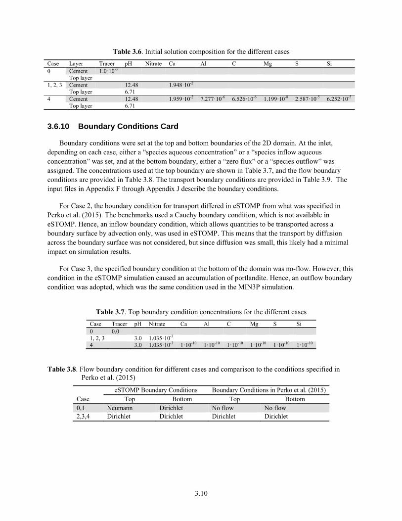
3.10
Table 3.6. Initial solution composition for the different cases
Case Layer Tracer pH Nitrate Ca Al C Mg S Si 0 Cement 1.0·10-3
Top layer 1, 2, 3 Cement 12.48 1.948·10-2
Top layer 6.71 4 Cement 12.48 1.959·10-2 7.277·10-6 6.526·10-6 1.199·10-8 2.587·10-5 6.252·10-5
Top layer 6.71
3.6.10 Boundary Conditions Card
Boundary conditions were set at the top and bottom boundaries of the 2D domain. At the inlet, depending on each case, either a “species aqueous concentration” or a “species inflow aqueous concentration” was set, and at the bottom boundary, either a “zero flux” or a “species outflow” was assigned. The concentrations used at the top boundary are shown in Table 3.7, and the flow boundary conditions are provided in Table 3.8. The transport boundary conditions are provided in Table 3.9. The input files in Appendix F through Appendix J describe the boundary conditions.
For Case 2, the boundary condition for transport differed in eSTOMP from what was specified in Perko et al. (2015). The benchmarks used a Cauchy boundary condition, which is not available in eSTOMP. Hence, an inflow boundary condition, which allows quantities to be transported across a boundary surface by advection only, was used in eSTOMP. This means that the transport by diffusion across the boundary surface was not considered, but since diffusion was small, this likely had a minimal impact on simulation results.
For Case 3, the specified boundary condition at the bottom of the domain was no-flow. However, this condition in the eSTOMP simulation caused an accumulation of portlandite. Hence, an outflow boundary condition was adopted, which was the same condition used in the MIN3P simulation.
Table 3.7. Top boundary condition concentrations for the different cases
Case Tracer pH Nitrate Ca Al C Mg S Si 0 0.0 1, 2, 3 3.0 1.035·10-3 4 3.0 1.035·10-3 1·10-10 1·10-10 1·10-10 1·10-10 1·10-10 1·10-10
Table 3.8. Flow boundary condition for different cases and comparison to the conditions specified in Perko et al. (2015)
Case eSTOMP Boundary Conditions Boundary Conditions in Perko et al. (2015)
Top Bottom Top Bottom 0,1 Neumann Dirichlet No flow No flow 2,3,4 Dirichlet Dirichlet Dirichlet Dirichlet
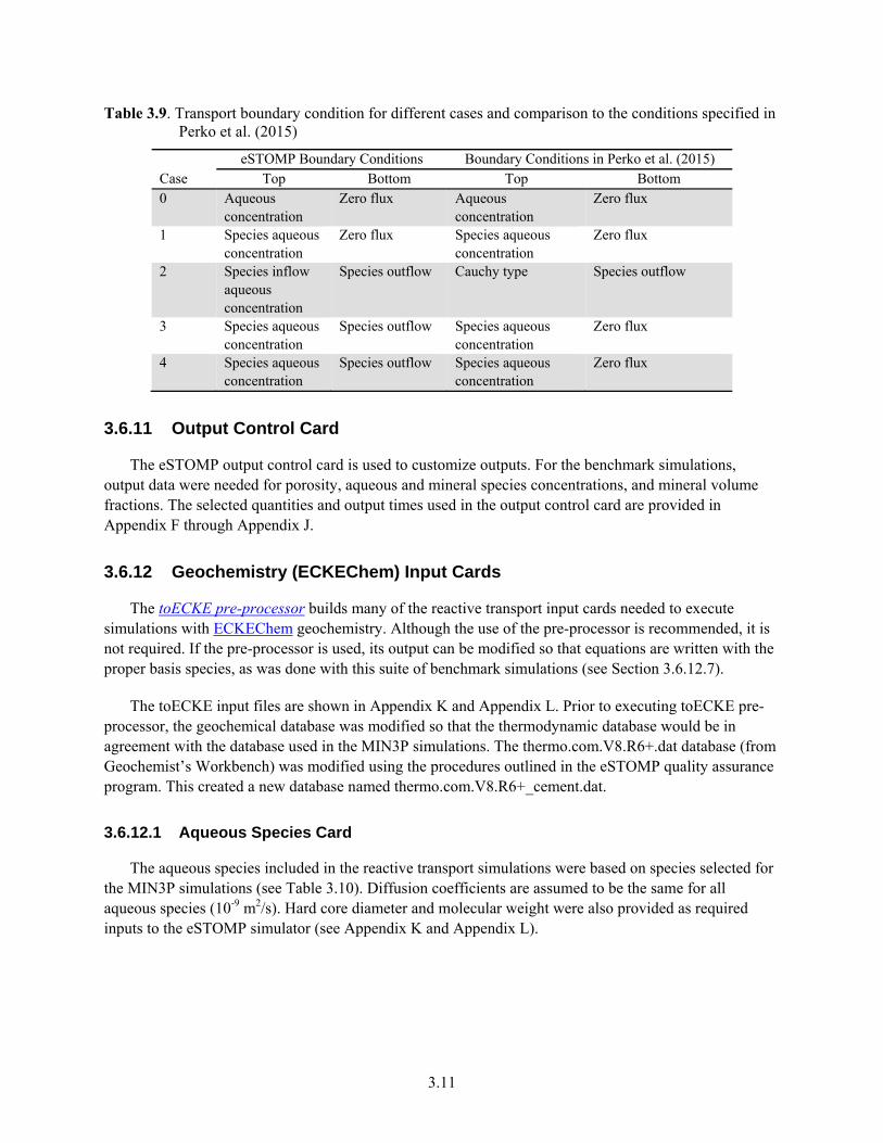
3.11
Table 3.9. Transport boundary condition for different cases and comparison to the conditions specified in Perko et al. (2015)
Case eSTOMP Boundary Conditions Boundary Conditions in Perko et al. (2015)
Top Bottom Top Bottom 0 Aqueous
concentration Zero flux Aqueous
concentration Zero flux
1 Species aqueous concentration
Zero flux Species aqueous concentration
Zero flux
2 Species inflow aqueous concentration
Species outflow Cauchy type Species outflow
3 Species aqueous concentration
Species outflow Species aqueous concentration
Zero flux
4 Species aqueous concentration
Species outflow Species aqueous concentration
Zero flux
3.6.11 Output Control Card
The eSTOMP output control card is used to customize outputs. For the benchmark simulations, output data were needed for porosity, aqueous and mineral species concentrations, and mineral volume fractions. The selected quantities and output times used in the output control card are provided in Appendix F through Appendix J.
3.6.12 Geochemistry (ECKEChem) Input Cards
The toECKE pre-processor builds many of the reactive transport input cards needed to execute simulations with ECKEChem geochemistry. Although the use of the pre-processor is recommended, it is not required. If the pre-processor is used, its output can be modified so that equations are written with the proper basis species, as was done with this suite of benchmark simulations (see Section 3.6.12.7).
The toECKE input files are shown in Appendix K and Appendix L. Prior to executing toECKE pre-processor, the geochemical database was modified so that the thermodynamic database would be in agreement with the database used in the MIN3P simulations. The thermo.com.V8.R6+.dat database (from Geochemist’s Workbench) was modified using the procedures outlined in the eSTOMP quality assurance program. This created a new database named thermo.com.V8.R6+_cement.dat.
3.6.12.1 Aqueous Species Card
The aqueous species included in the reactive transport simulations were based on species selected for the MIN3P simulations (see Table 3.10). Diffusion coefficients are assumed to be the same for all aqueous species (10-9 m2/s). Hard core diameter and molecular weight were also provided as required inputs to the eSTOMP simulator (see Appendix K and Appendix L).
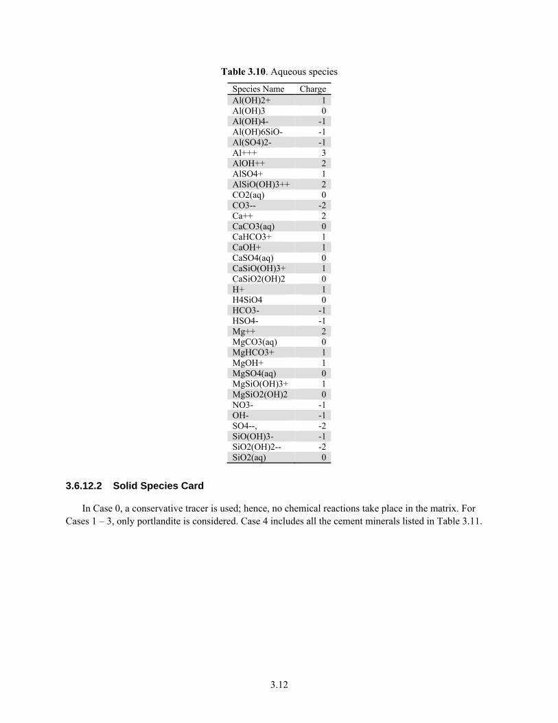
3.12
Table 3.10. Aqueous species
Species Name Charge Al(OH)2+ 1 Al(OH)3 0 Al(OH)4- -1 Al(OH)6SiO- -1 Al(SO4)2- -1 Al+++ 3 AlOH++ 2 AlSO4+ 1 AlSiO(OH)3++ 2 CO2(aq) 0 CO3-- -2 Ca++ 2 CaCO3(aq) 0 CaHCO3+ 1 CaOH+ 1 CaSO4(aq) 0 CaSiO(OH)3+ 1 CaSiO2(OH)2 0 H+ 1 H4SiO4 0 HCO3- -1 HSO4- -1 Mg++ 2 MgCO3(aq) 0 MgHCO3+ 1 MgOH+ 1 MgSO4(aq) 0 MgSiO(OH)3+ 1 MgSiO2(OH)2 0 NO3- -1 OH- -1 SO4--, -2 SiO(OH)3- -1 SiO2(OH)2-- -2 SiO2(aq) 0
3.6.12.2 Solid Species Card
In Case 0, a conservative tracer is used; hence, no chemical reactions take place in the matrix. For Cases 1 – 3, only portlandite is considered. Case 4 includes all the cement minerals listed in Table 3.11.
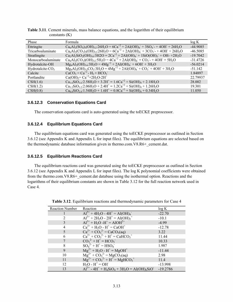
3.13
Table 3.11. Cement minerals, mass balance equations, and the logarithm of their equilibrium constants (K)
Phase Formula log K Ettringite Ca6Al2(SO4)3(OH)12:26H2O = 6Ca+2 + 2Al(OH)4
- + 3SO4-- + 4OH- + 26H2O -44.9085
Tricarboaluminate Ca6Al2(CO3)3(OH)12:26H2O = 6Ca+2 + 2Al(OH)4- + 3CO3
-- + 4OH- + 26H2O -46.5085 Stratlingite Ca2Al2SiO2(OH)10:3H2O = 2Ca+2 + 2Al(OH)4
- + 1SiO(OH)3- + OH- +2H2O -19.7042
Monocarboaluminate Ca4Al2(CO3)(OH)12:5H2O = 4Ca+2 + 2Al(OH)4- + CO3
-- + 4OH- + 5H2O -31.4726 Hydrotalcite-OH Mg4Al2(OH)14:3H2O = 4Mg+2 + 2Al(OH)4
- + 6OH- + 3H2O -56.0214 Hydrotalcite-CO3 Mg4Al2(OH)12CO3:3H2O = 4Mg+2 + 2Al(OH)4
- + CO3- + 4OH- + 3H2O -51.142
Calcite CaCO3 = Ca+2 - H2 + HCO3- 1.84897
Portlandite Ca(OH)2= Ca+2+2H2O-2H+ 22.79937 CSH(1.6) Ca1.6SiO3.6:2.58H2O + 3.2H+ = 1.6Ca+2 + Si(OH)4 + 2.18H2O 28.002 CSH(1.2) Ca1.2SiO3.2:2.06H2O + 2.4H+ = 1.2Ca+2 + Si(OH)4 + 1.26H2O 19.301 CSH(0.8) Ca0.8SiO2.8:1.54H2O + 1.6H+ = 0.8Ca+2 + Si(OH)4 + 0.34H2O 11.050
3.6.12.3 Conservation Equations Card
The conservation equations card is auto-generated using the toECKE preprocessor.
3.6.12.4 Equilibrium Equations Card
The equilibrium equations card was generated using the toECKE preprocessor as outlined in Section 3.6.12 (see Appendix K and Appendix L for input files). The equilibrium equations are selected based on the thermodynamic database information given in thermo.com.V8.R6+_cement.dat.
3.6.12.5 Equilibrium Reactions Card
The equilibrium reactions card was generated using the toECKE preprocessor as outlined in Section 3.6.12 (see Appendix K and Appendix L for input files). The log K polynomial coefficients were obtained from the thermo.com.V8.R6+_cement.dat database using the isothermal option. Reactions and the logarithms of their equilibrium constants are shown in Table 3.12 for the full reaction network used in Case 4.
Table 3.12. Equilibrium reactions and thermodynamic parameters for Case 4
Reaction Number Reaction log K 1 Al3+ + 4H2O - 4H+ = Al(OH)4
- -22.70 2 Al3+ + 2H2O - 2H+ = Al(OH)2
+ -10.1 3 Al3+ + H2O -H+ = AlOH2+ -4.99 4 Ca2+ + H2O - H+ = CaOH+ -12.78 5 Ca2+ + CO3
2- = CaCO3(aq) 3.22 6 Ca2+ + CO3
2- + H+ = CaHCO3+ 11.44
7 CO32- + H+ = HCO3
- 10.33 8 SO4
2- + H+ = HSO4- 1.987
9 Mg2+ + H2O - H+ = MgOH+ -11.44 10 Mg2+ + CO3
2- = MgCO3(aq) 2.98 11 Mg2+ + CO3
2- + H+ = MgHCO3+ 11.4
12 H2O - H+ = OH- -13.998 13 Al3+ - 4H+ + H4SiO4 + 3H2O = Al(OH)6SiO- -19.2786
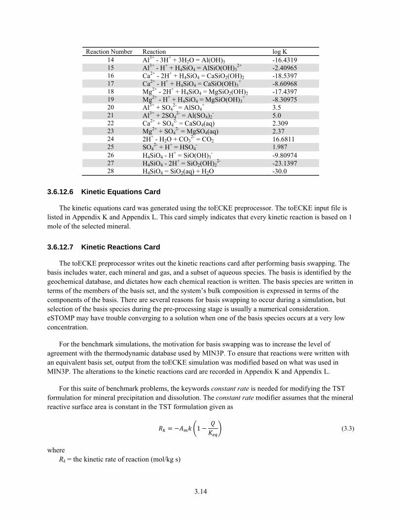
3.14
Reaction Number Reaction log K 14 Al3+ - 3H+ + 3H2O = Al(OH)3 -16.4319 15 Al3+ - H+ + H4SiO4 = AlSiO(OH)3
2+ -2.40965 16 Ca2+ - 2H+ + H4SiO4 = CaSiO2(OH)2 -18.5397 17 Ca2+ - H+ + H4SiO4 = CaSiO(OH)3
+ -8.60968 18 Mg2+ - 2H+ + H4SiO4 = MgSiO2(OH)2 -17.4397 19 Mg2+ - H+ + H4SiO4 = MgSiO(OH)3
+ -8.30975 20 Al3+ + SO4
2- = AlSO4+ 3.5
21 Al3+ + 2SO42- = Al(SO4)2
- 5.0 22 Ca2+ + SO4
2- = CaSO4(aq) 2.309 23 Mg2+ + SO4
2- = MgSO4(aq) 2.37 24 2H+ - H2O + CO3
2- = CO2 16.6811 25 SO4
2- + H+ = HSO4- 1.987
26 H4SiO4 - H+ = SiO(OH)3
- -9.80974 27 H4SiO4 - 2H+ = SiO2(OH)2
2- -23.1397 28 H4SiO4 = SiO2(aq) + H2O -30.0
3.6.12.6 Kinetic Equations Card
The kinetic equations card was generated using the toECKE preprocessor. The toECKE input file is listed in Appendix K and Appendix L. This card simply indicates that every kinetic reaction is based on 1 mole of the selected mineral.
3.6.12.7 Kinetic Reactions Card
The toECKE preprocessor writes out the kinetic reactions card after performing basis swapping. The basis includes water, each mineral and gas, and a subset of aqueous species. The basis is identified by the geochemical database, and dictates how each chemical reaction is written. The basis species are written in terms of the members of the basis set, and the system’s bulk composition is expressed in terms of the components of the basis. There are several reasons for basis swapping to occur during a simulation, but selection of the basis species during the pre-processing stage is usually a numerical consideration. eSTOMP may have trouble converging to a solution when one of the basis species occurs at a very low concentration.
For the benchmark simulations, the motivation for basis swapping was to increase the level of agreement with the thermodynamic database used by MIN3P. To ensure that reactions were written with an equivalent basis set, output from the toECKE simulation was modified based on what was used in MIN3P. The alterations to the kinetic reactions card are recorded in Appendix K and Appendix L.
For this suite of benchmark problems, the keywords constant rate is needed for modifying the TST formulation for mineral precipitation and dissolution. The constant rate modifier assumes that the mineral reactive surface area is constant in the TST formulation given as
1 (3.3)
where Rk = the kinetic rate of reaction (mol/kg s)
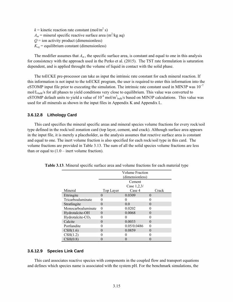
3.15
k = kinetic reaction rate constant (mol/m2 s) Am = mineral specific reactive surface area (m2/kg aq) Q = ion activity product (dimensionless) Keq = equilibrium constant (dimensionless)
The modifier assumes that Am , the specific surface area, is constant and equal to one in this analysis for consistency with the approach used in the Perko et al. (2015). The TST rate formulation is saturation dependent, and is applied throught the volume of liquid in contact with the solid phase.
The toECKE pre-processor can take as input the intrinsic rate constant for each mineral reaction. If this information is not input to the toECKE program, the user is required to enter this information into the eSTOMP input file prior to executing the simulation. The intrinsic rate constant used in MIN3P was 10−7 mol/Lbulk/s for all phases to yield conditions very close to equilibrium. This value was converted to eSTOMP default units to yield a value of 10-4 mol/m3
bulk/s based on MIN3P calculations. This value was used for all minerals as shown in the input files in Appendix K and Appendix L.
3.6.12.8 Lithology Card
This card specifies the mineral specific areas and mineral species volume fractions for every rock/soil type defined in the rock/soil zonation card (top layer, cement, and crack). Although surface area appears in the input file, it is merely a placeholder, as the analysis assumes that reactive surface area is constant and equal to one. The inert volume fraction is also specified for each rock/soil type in this card. The volume fractions are provided in Table 3.13. The sum of all the solid species volume fractions are less than or equal to (1.0 – inert volume fraction).
Table 3.13. Mineral specific surface area and volume fractions for each material type
Mineral
Volume Fraction(dimensionless)
Top Layer
CementCase 1,2,3/
Case 4 Crack Ettringite 0 0.0309 0 Tricarboaluminate 0 0 0 Stratlingite 0 0.0 0 Monocarboaluminate 0 0.0202 0 Hydrotalcite-OH 0 0.0068 0 Hydrotalcite-CO3 0 0 0 Calcite 0 0.0033 0 Portlandite 0 0.05/0.0486 0 CSH(1.6) 0 0.0859 0 CSH(1.2) 0 0 0 CSH(0.8) 0 0 0
3.6.12.9 Species Link Card
This card associates reactive species with components in the coupled flow and transport equations and defines which species name is associated with the system pH. For the benchmark simulations, the
3.16
species link card is used so that pH (i.e., H+ activity) can be used to describe the initial condition, rather than H+ aqueous concentration.
3.7 Simulation Results
Simulation results are presented at 100 years for pH, calcium concentration, and fields of portlandite for all of the benchmark simulations. These profiles of Ca2+ pH and portlandite are provided for the cross-sections shown in Figure 3.1. These quantities are used in the comparison because the pH influences the dissolution rate of the cementitious waste, and aqueous calcium concentrations follow the portlandite concentrations because calcium concentrations are buffered by portlandite. When porosity updates are considered, a comparison of those results is also provided. In the final case, additional minerals are included in the cementitious waste form and those volume fractions are also used for comparison to eSTOMP simulation results.
The benchmark is presented as a series of six consecutive cases with increasing complexity. Cases 0 and 1 deal with diffusive transport only. The diffusive transport regime corresponds to a fresh hardened cement paste (Cast Stone) condition because of a very low hydraulic conductivity. Case 2 deals with advective transport, which is relevant for (partially) degraded Cast Stone. Evolution from diffusive to advective conditions is tackled in Case 3, where Cast Stone transport properties are altered as a function of the geochemical state variables during chemical alterations. Case 4 introduces a more complex and realistic geochemical system. Whereas Case 3 assumes that only portlandite is present, Case 4 not only includes portlandite, but several other cement minerals.
3.7.1 Case 0: Conservative Tracer
The main purpose of Case 0, the simplest of all of the benchmark simulations, is to ensure that the implementation of a single crack is done correctly for a purely diffusive system using a conservatively transported tracer (i.e., no reactions). The 5 cm × 10 cm domain is discretized into 101 and 105 grid cells in the x- and z-directions, respectively, to evaluate the diffusion caused by the crack. Grid spacing varies from 0.125 to 0.25 mm in the x-direction and 0.5 to 1.5 mm in the z direction. The starting time step is 1 s and maximum time step is 0.1 d. The cement area including the crack has a uniform initial concentration of the tracer of 10−3 mol/L. The top layer, defined with a 5-mm thickness, initially has a zero tracer concentration. The top boundary condition is also defined as a constant zero concentration boundary condition. All other boundaries (sides and bottom) are zero flux and zero concentration boundary conditions. The initial and boundary conditions are shown in Figure 3.2 and summarized in Table 3.6 – Table 3.9.
Figure 3.5 shows the comparison of tracer concentrations for eSTOMP and the simulators reporting results in Perko et al. (2015) along the horizontal and vertical profiles shown in Figure 3.1 after 100 days (see select locations in Figure 3.1). The effective diffusion in the crack is higher than in the cement, as noted in the adjacent vertical profile (Figure 3.5b). Hence, the vertical concentration gradient in the cement adjacent to the crack is lower. All codes show that the concentration gradients are affected by the high diffusion crack zone. Higher diffusion in the crack caused tracer redistribution with higher vertical gradients at the boundary and lower vertical gradients close to the crack. The influence of the crack diminishes with distance from the crack. Model results vary a bit near the crack region in both profiles, possibly due to grid discretization (e.g., SC3K used a coarser grid) and numerical formulations.
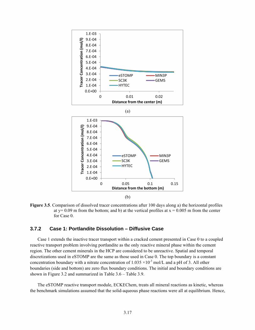
3.17
(a)
(b)
Figure 3.5. Comparison of dissolved tracer concentrations after 100 days along a) the horizontal profiles at y= 0.09 m from the bottom; and b) at the vertical profiles at x = 0.005 m from the center for Case 0.
3.7.2 Case 1: Portlandite Dissolution – Diffusive Case
Case 1 extends the inactive tracer transport within a cracked cement presented in Case 0 to a coupled reactive transport problem involving portlandite as the only reactive mineral phase within the cement region. The other cement minerals in the HCP are considered to be unreactive. Spatial and temporal discretizations used in eSTOMP are the same as those used in Case 0. The top boundary is a constant concentration boundary with a nitrate concentration of 1.035 ×10⁻³ mol/L and a pH of 3. All other boundaries (side and bottom) are zero flux boundary conditions. The initial and boundary conditions are shown in Figure 3.2 and summarized in Table 3.6 – Table 3.9.
The eSTOMP reactive transport module, ECKEChem, treats all mineral reactions as kinetic, whereas the benchmark simulations assumed that the solid-aqueous phase reactions were all at equilibrium. Hence,
0.E+00
1.E‐04
2.E‐04
3.E‐04
4.E‐04
5.E‐04
6.E‐04
7.E‐04
8.E‐04
9.E‐04
1.E‐03
0 0.01 0.02
Tracer Concentration (mol/l)
Distance from the center (m)
eSTOMP MIN3PSC3K GEMSHYTEC
0.E+00
1.E‐04
2.E‐04
3.E‐04
4.E‐04
5.E‐04
6.E‐04
7.E‐04
8.E‐04
9.E‐04
1.E‐03
0 0.05 0.1 0.15
Tracer Concentration (mol/l)
Distance from the bottom (m)
eSTOMP MIN3PSC3K GEMSHYTEC
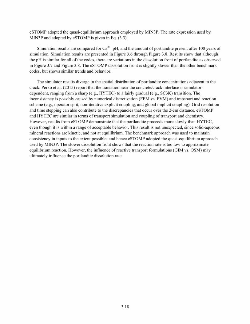
3.18
eSTOMP adopted the quasi-equilibrium approach employed by MIN3P. The rate expression used by MIN3P and adopted by eSTOMP is given in Eq. (3.3).
Simulation results are compared for Ca2+, pH, and the amount of portlandite present after 100 years of simulation. Simulation results are presented in Figure 3.6 through Figure 3.8. Results show that although the pH is similar for all of the codes, there are variations in the dissolution front of portlandite as observed in Figure 3.7 and Figure 3.8. The eSTOMP dissolution front is slightly slower than the other benchmark codes, but shows similar trends and behavior.
The simulator results diverge in the spatial distribution of portlandite concentrations adjacent to the crack. Perko et al. (2015) report that the transition near the concrete/crack interface is simulator-dependent, ranging from a sharp (e.g., HYTEC) to a fairly gradual (e.g., SC3K) transition. The inconsistency is possibly caused by numerical discretization (FEM vs. FVM) and transport and reaction scheme (e.g., operator split, non-iterative explicit coupling, and global implicit coupling). Grid resolution and time stepping can also contribute to the discrepancies that occur over the 2-cm distance. eSTOMP and HYTEC are similar in terms of transport simulation and coupling of transport and chemistry. However, results from eSTOMP demonstrate that the portlandite proceeds more slowly than HYTEC, even though it is within a range of acceptable behavior. This result is not unexpected, since solid-aqueous mineral reactions are kinetic, and not at equilibrium. The benchmark approach was used to maintain consistency in inputs to the extent possible, and hence eSTOMP adopted the quasi-equilibrium approach used by MIN3P. The slower dissolution front shows that the reaction rate is too low to approximate equilibrium reaction. However, the influence of reactive transport formulations (GIM vs. OSM) may ultimately influence the portlandite dissolution rate.
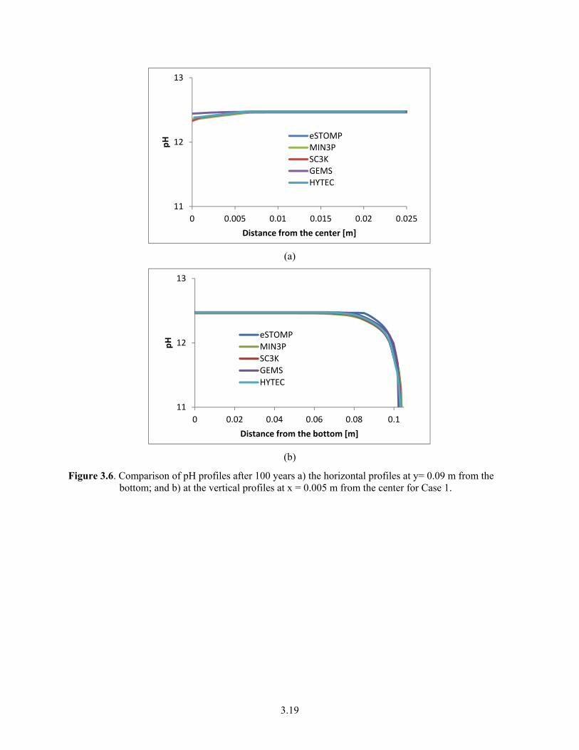
3.19
(a)
(b)
Figure 3.6. Comparison of pH profiles after 100 years a) the horizontal profiles at y= 0.09 m from the bottom; and b) at the vertical profiles at x = 0.005 m from the center for Case 1.
11
12
13
0 0.005 0.01 0.015 0.02 0.025
pH
Distance from the center [m]
eSTOMPMIN3PSC3KGEMSHYTEC
11
12
13
0 0.02 0.04 0.06 0.08 0.1
pH
Distance from the bottom [m]
eSTOMP
MIN3P
SC3K
GEMS
HYTEC
3.20
(a)
(b)
Figure 3.7. Comparison of Ca2+ profiles after 100 years a) the horizontal profiles at y= 0.09 m from the bottom; and b) at the vertical profiles at x = 0.005 m from the center for Case 1.
0.0E+00
5.0E‐03
1.0E‐02
1.5E‐02
2.0E‐02
2.5E‐02
0 0.005 0.01 0.015 0.02 0.025
Ca++ [m
ol/l]
Distance from the center [m]
eSTOMP
MIN3P
SC3K
GEMS
HYTEC
0.0E+00
5.0E‐03
1.0E‐02
1.5E‐02
2.0E‐02
2.5E‐02
0 0.02 0.04 0.06 0.08 0.1
Ca++ [m
ol/l)
Distance from the bottom [m]
eSTOMP
MIN3P
SC3K
GEMS
HYTEC
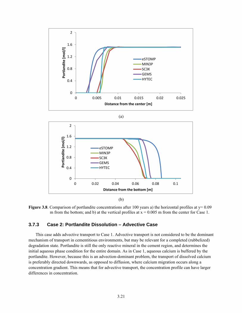
3.21
(a)
(b)
Figure 3.8. Comparison of portlandite concentrations after 100 years a) the horizontal profiles at y= 0.09 m from the bottom; and b) at the vertical profiles at x = 0.005 m from the center for Case 1.
3.7.3 Case 2: Portlandite Dissolution – Advective Case
This case adds advective transport to Case 1. Advective transport is not considered to be the dominant mechanism of transport in cementitious environments, but may be relevant for a completed (rubbelized) degradation state. Portlandite is still the only reactive mineral in the cement region, and determines the initial aqueous phase condition for the entire domain. As in Case 1, aqueous calcium is buffered by the portlandite. However, because this is an advection-dominant problem, the transport of dissolved calcium is preferably directed downwards, as opposed to diffusion, where calcium migration occurs along a concentration gradient. This means that for advective transport, the concentration profile can have larger differences in concentration.
0
0.4
0.8
1.2
1.6
2
0 0.005 0.01 0.015 0.02 0.025
Portlandite [m
ol/l]
Distance from the center [m]
eSTOMP
MIN3P
SC3K
GEMS
HYTEC
0
0.4
0.8
1.2
1.6
2
0 0.02 0.04 0.06 0.08 0.1
Portlandite [mol/l)
Distance from the bottom [m]
eSTOMPMIN3PSC3KGEMSHYTEC
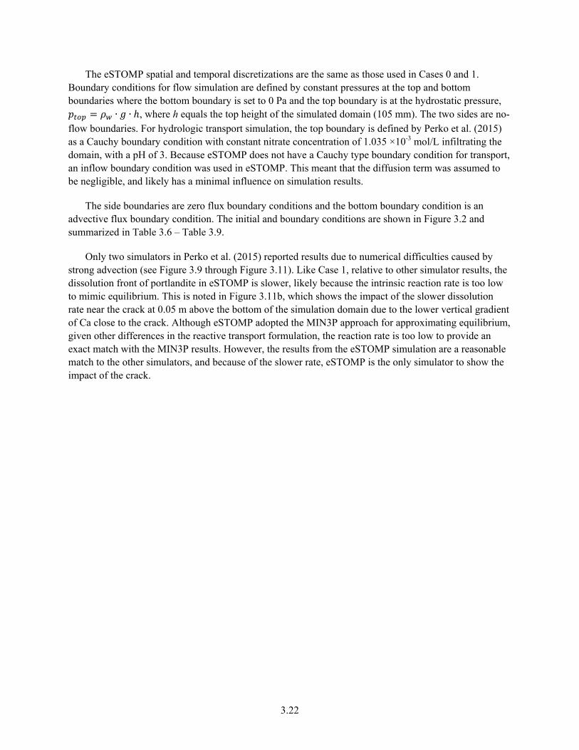
3.22
The eSTOMP spatial and temporal discretizations are the same as those used in Cases 0 and 1. Boundary conditions for flow simulation are defined by constant pressures at the top and bottom boundaries where the bottom boundary is set to 0 Pa and the top boundary is at the hydrostatic pressure,
∙ ∙ , where h equals the top height of the simulated domain (105 mm). The two sides are no-flow boundaries. For hydrologic transport simulation, the top boundary is defined by Perko et al. (2015) as a Cauchy boundary condition with constant nitrate concentration of 1.035 ×10⁻³ mol/L infiltrating the domain, with a pH of 3. Because eSTOMP does not have a Cauchy type boundary condition for transport, an inflow boundary condition was used in eSTOMP. This meant that the diffusion term was assumed to be negligible, and likely has a minimal influence on simulation results.
The side boundaries are zero flux boundary conditions and the bottom boundary condition is an advective flux boundary condition. The initial and boundary conditions are shown in Figure 3.2 and summarized in Table 3.6 – Table 3.9.
Only two simulators in Perko et al. (2015) reported results due to numerical difficulties caused by strong advection (see Figure 3.9 through Figure 3.11). Like Case 1, relative to other simulator results, the dissolution front of portlandite in eSTOMP is slower, likely because the intrinsic reaction rate is too low to mimic equilibrium. This is noted in Figure 3.11b, which shows the impact of the slower dissolution rate near the crack at 0.05 m above the bottom of the simulation domain due to the lower vertical gradient of Ca close to the crack. Although eSTOMP adopted the MIN3P approach for approximating equilibrium, given other differences in the reactive transport formulation, the reaction rate is too low to provide an exact match with the MIN3P results. However, the results from the eSTOMP simulation are a reasonable match to the other simulators, and because of the slower rate, eSTOMP is the only simulator to show the impact of the crack.
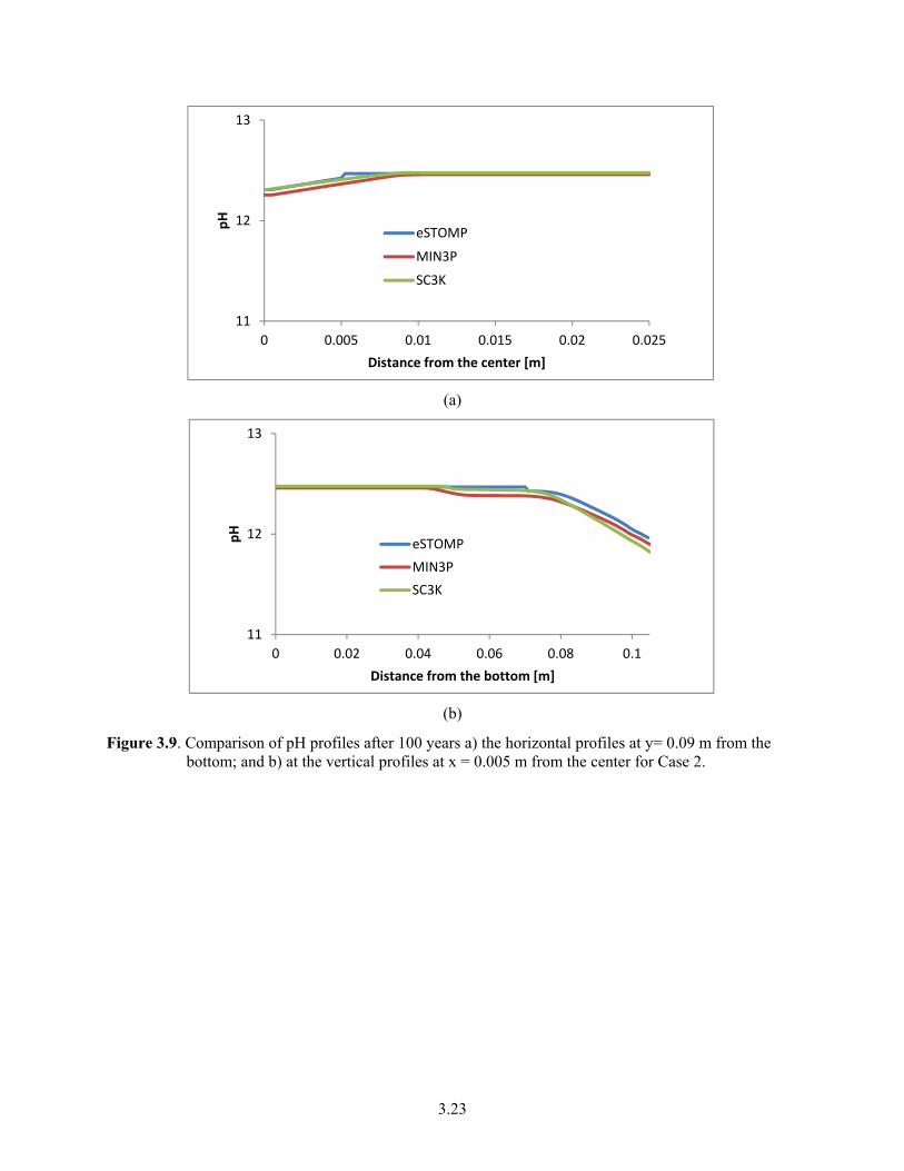
3.23
(a)
(b)
Figure 3.9. Comparison of pH profiles after 100 years a) the horizontal profiles at y= 0.09 m from the bottom; and b) at the vertical profiles at x = 0.005 m from the center for Case 2.
11
12
13
0 0.005 0.01 0.015 0.02 0.025
pH
Distance from the center [m]
eSTOMP
MIN3P
SC3K
11
12
13
0 0.02 0.04 0.06 0.08 0.1
pH
Distance from the bottom [m]
eSTOMP
MIN3P
SC3K
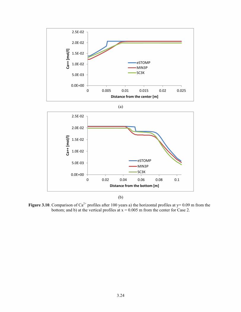
3.24
(a)
(b)
Figure 3.10. Comparison of Ca2+ profiles after 100 years a) the horizontal profiles at y= 0.09 m from the bottom; and b) at the vertical profiles at x = 0.005 m from the center for Case 2.
0.0E+00
5.0E‐03
1.0E‐02
1.5E‐02
2.0E‐02
2.5E‐02
0 0.005 0.01 0.015 0.02 0.025
Ca++ [m
ol/l]
Distance from the center [m]
eSTOMP
MIN3P
SC3K
0.0E+00
5.0E‐03
1.0E‐02
1.5E‐02
2.0E‐02
2.5E‐02
0 0.02 0.04 0.06 0.08 0.1
Ca++ [m
ol/l)
Distance from the bottom [m]
eSTOMP
MIN3P
SC3K
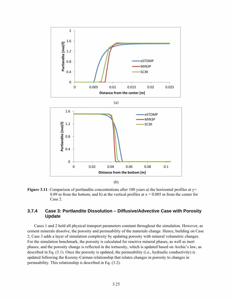
3.25
(a)
(b)
Figure 3.11. Comparison of portlandite concentrations after 100 years a) the horizontal profiles at y= 0.09 m from the bottom; and b) at the vertical profiles at x = 0.005 m from the center for Case 2.
3.7.4 Case 3: Portlandite Dissolution – Diffusive/Advective Case with Porosity Update
Cases 1 and 2 held all physical transport parameters constant throughout the simulation. However, as cement minerals dissolve, the porosity and permeability of the materials change. Hence, building on Case 2, Case 3 adds a layer of simulation complexity by updating porosity with mineral volumetric changes. For the simulation benchmark, the porosity is calculated for reactive mineral phases, as well as inert phases, and the porosity change is reflected in the tortuosity, which is updated based on Archie’s law, as described in Eq. (3.1). Once the porosity is updated, the permeability (i.e., hydraulic conductivity) is updated following the Kozeny-Carman relationship that relates changes in porosity to changes in permeability. This relationship is described in Eq. (3.2).
0
0.4
0.8
1.2
1.6
2
0 0.005 0.01 0.015 0.02 0.025
Portlandite [m
ol/l]
Distance from the center [m]
eSTOMP
MIN3P
SC3K
0
0.4
0.8
1.2
1.6
0 0.02 0.04 0.06 0.08 0.1
Portlandite [mol/l)
Distance from the bottom [m]
eSTOMP
MIN3P
SC3K
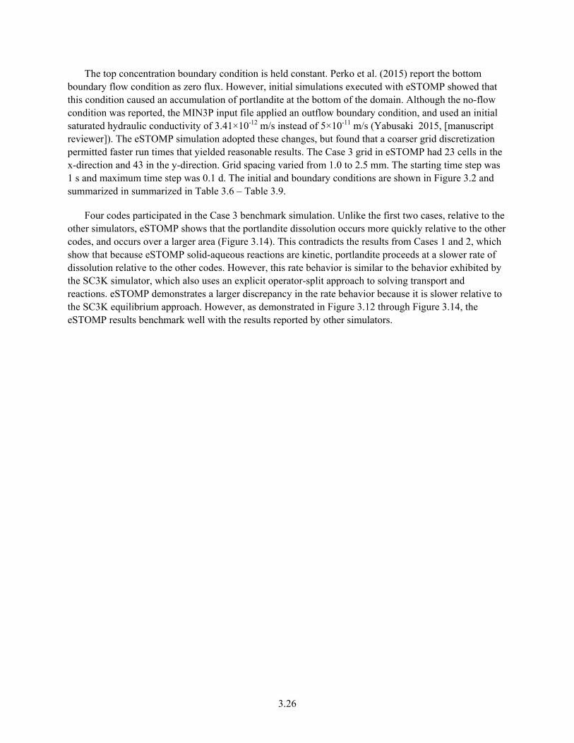
3.26
The top concentration boundary condition is held constant. Perko et al. (2015) report the bottom boundary flow condition as zero flux. However, initial simulations executed with eSTOMP showed that this condition caused an accumulation of portlandite at the bottom of the domain. Although the no-flow condition was reported, the MIN3P input file applied an outflow boundary condition, and used an initial saturated hydraulic conductivity of 3.41×10⁻¹² m/s instead of 5×10-11 m/s (Yabusaki 2015, [manuscript reviewer]). The eSTOMP simulation adopted these changes, but found that a coarser grid discretization permitted faster run times that yielded reasonable results. The Case 3 grid in eSTOMP had 23 cells in the x-direction and 43 in the y-direction. Grid spacing varied from 1.0 to 2.5 mm. The starting time step was 1 s and maximum time step was 0.1 d. The initial and boundary conditions are shown in Figure 3.2 and summarized in summarized in Table 3.6 – Table 3.9.
Four codes participated in the Case 3 benchmark simulation. Unlike the first two cases, relative to the other simulators, eSTOMP shows that the portlandite dissolution occurs more quickly relative to the other codes, and occurs over a larger area (Figure 3.14). This contradicts the results from Cases 1 and 2, which show that because eSTOMP solid-aqueous reactions are kinetic, portlandite proceeds at a slower rate of dissolution relative to the other codes. However, this rate behavior is similar to the behavior exhibited by the SC3K simulator, which also uses an explicit operator-split approach to solving transport and reactions. eSTOMP demonstrates a larger discrepancy in the rate behavior because it is slower relative to the SC3K equilibrium approach. However, as demonstrated in Figure 3.12 through Figure 3.14, the eSTOMP results benchmark well with the results reported by other simulators.
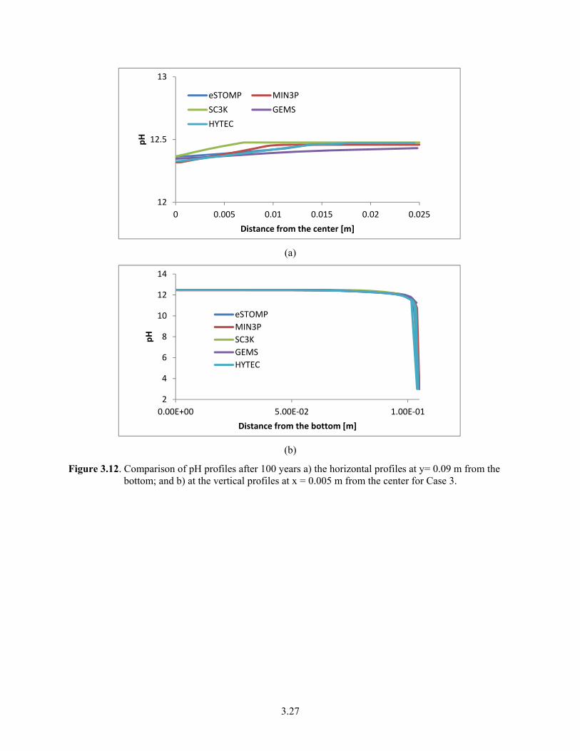
3.27
(a)
(b)
Figure 3.12. Comparison of pH profiles after 100 years a) the horizontal profiles at y= 0.09 m from the bottom; and b) at the vertical profiles at x = 0.005 m from the center for Case 3.
12
12.5
13
0 0.005 0.01 0.015 0.02 0.025
pH
Distance from the center [m]
eSTOMP MIN3P
SC3K GEMS
HYTEC
2
4
6
8
10
12
14
0.00E+00 5.00E‐02 1.00E‐01
pH
Distance from the bottom [m]
eSTOMP
MIN3P
SC3K
GEMS
HYTEC
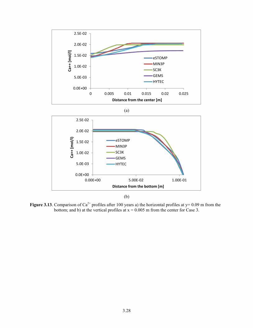
3.28
(a)
(b)
Figure 3.13. Comparison of Ca2+ profiles after 100 years a) the horizontal profiles at y= 0.09 m from the bottom; and b) at the vertical profiles at x = 0.005 m from the center for Case 3.
0.0E+00
5.0E‐03
1.0E‐02
1.5E‐02
2.0E‐02
2.5E‐02
0 0.005 0.01 0.015 0.02 0.025
Ca++ [m
ol/l]
Distance from the center [m]
eSTOMP
MIN3P
SC3K
GEMS
HYTEC
0.0E+00
5.0E‐03
1.0E‐02
1.5E‐02
2.0E‐02
2.5E‐02
0.00E+00 5.00E‐02 1.00E‐01
Ca++ [m
ol/l)
Distance from the bottom [m]
eSTOMP
MIN3P
SC3K
GEMS
HYTEC
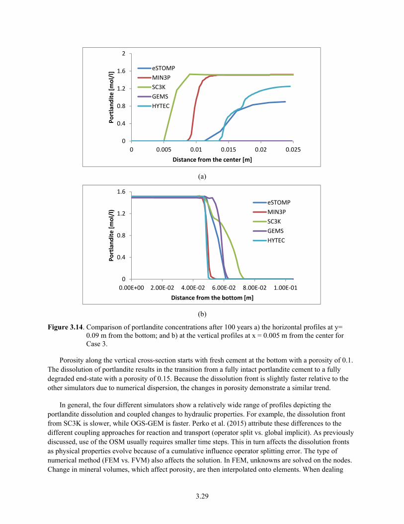
3.29
(a)
(b)
Figure 3.14. Comparison of portlandite concentrations after 100 years a) the horizontal profiles at y= 0.09 m from the bottom; and b) at the vertical profiles at x = 0.005 m from the center for Case 3.
Porosity along the vertical cross-section starts with fresh cement at the bottom with a porosity of 0.1. The dissolution of portlandite results in the transition from a fully intact portlandite cement to a fully degraded end-state with a porosity of 0.15. Because the dissolution front is slightly faster relative to the other simulators due to numerical dispersion, the changes in porosity demonstrate a similar trend.
In general, the four different simulators show a relatively wide range of profiles depicting the portlandite dissolution and coupled changes to hydraulic properties. For example, the dissolution front from SC3K is slower, while OGS-GEM is faster. Perko et al. (2015) attribute these differences to the different coupling approaches for reaction and transport (operator split vs. global implicit). As previously discussed, use of the OSM usually requires smaller time steps. This in turn affects the dissolution fronts as physical properties evolve because of a cumulative influence operator splitting error. The type of numerical method (FEM vs. FVM) also affects the solution. In FEM, unknowns are solved on the nodes. Change in mineral volumes, which affect porosity, are then interpolated onto elements. When dealing
0
0.4
0.8
1.2
1.6
2
0 0.005 0.01 0.015 0.02 0.025
Portlandite [m
ol/l]
Distance from the center [m]
eSTOMP
MIN3P
SC3K
GEMS
HYTEC
0
0.4
0.8
1.2
1.6
0.00E+00 2.00E‐02 4.00E‐02 6.00E‐02 8.00E‐02 1.00E‐01
Portlandite [mol/l)
Distance from the bottom [m]
eSTOMP
MIN3P
SC3K
GEMS
HYTEC
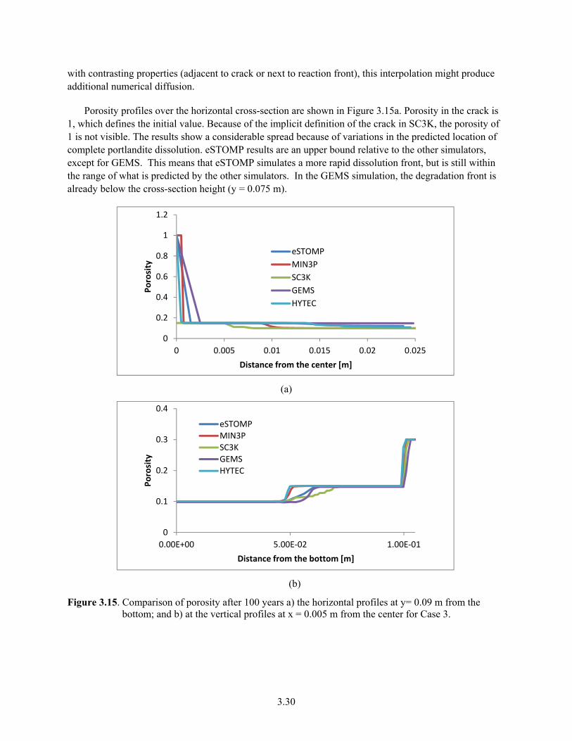
3.30
with contrasting properties (adjacent to crack or next to reaction front), this interpolation might produce additional numerical diffusion.
Porosity profiles over the horizontal cross-section are shown in Figure 3.15a. Porosity in the crack is 1, which defines the initial value. Because of the implicit definition of the crack in SC3K, the porosity of 1 is not visible. The results show a considerable spread because of variations in the predicted location of complete portlandite dissolution. eSTOMP results are an upper bound relative to the other simulators, except for GEMS. This means that eSTOMP simulates a more rapid dissolution front, but is still within the range of what is predicted by the other simulators. In the GEMS simulation, the degradation front is already below the cross-section height (y = 0.075 m).
(a)
(b)
Figure 3.15. Comparison of porosity after 100 years a) the horizontal profiles at y= 0.09 m from the bottom; and b) at the vertical profiles at x = 0.005 m from the center for Case 3.
0
0.2
0.4
0.6
0.8
1
1.2
0 0.005 0.01 0.015 0.02 0.025
Porosity
Distance from the center [m]
eSTOMP
MIN3P
SC3K
GEMS
HYTEC
0
0.1
0.2
0.3
0.4
0.00E+00 5.00E‐02 1.00E‐01
Porosity
Distance from the bottom [m]
eSTOMPMIN3PSC3KGEMSHYTEC
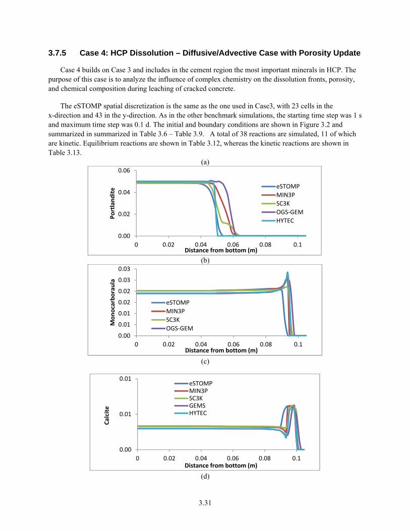
3.31
3.7.5 Case 4: HCP Dissolution – Diffusive/Advective Case with Porosity Update
Case 4 builds on Case 3 and includes in the cement region the most important minerals in HCP. The purpose of this case is to analyze the influence of complex chemistry on the dissolution fronts, porosity, and chemical composition during leaching of cracked concrete.
The eSTOMP spatial discretization is the same as the one used in Case3, with 23 cells in the x-direction and 43 in the y-direction. As in the other benchmark simulations, the starting time step was 1 s and maximum time step was 0.1 d. The initial and boundary conditions are shown in Figure 3.2 and summarized in summarized in Table 3.6 – Table 3.9. A total of 38 reactions are simulated, 11 of which are kinetic. Equilibrium reactions are shown in Table 3.12, whereas the kinetic reactions are shown in Table 3.13.
(a)
(b)
(c)
(d)
0.00
0.02
0.04
0.06
0 0.02 0.04 0.06 0.08 0.1
Portlandite
Distance from bottom (m)
eSTOMP
MIN3P
SC3K
OGS‐GEM
HYTEC
0.00
0.01
0.01
0.02
0.02
0.03
0.03
0 0.02 0.04 0.06 0.08 0.1
Monocarboraula
Distance from bottom (m)
eSTOMP
MIN3P
SC3K
OGS‐GEM
0.00
0.01
0.01
0 0.02 0.04 0.06 0.08 0.1
Calcite
Distance from bottom (m)
eSTOMPMIN3PSC3KGEMSHYTEC
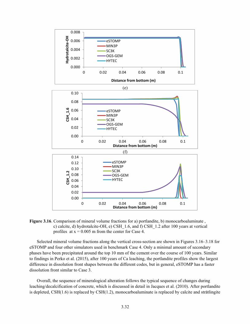
3.32
(e)
(f)
Figure 3.16. Comparison of mineral volume fractions for a) portlandite, b) monocarboaluminate , c) calcite, d) hydrotalcite-OH, e) CSH_1.6, and f) CSH_1.2 after 100 years at vertical profiles at x = 0.005 m from the center for Case 4.
Selected mineral volume fractions along the vertical cross-section are shown in Figures 3.16–3.18 for eSTOMP and four other simulators used in benchmark Case 4. Only a minimal amount of secondary phases have been precipitated around the top 10 mm of the cement over the course of 100 years. Similar to findings in Perko et al. (2015), after 100 years of Ca leaching, the portlandite profiles show the largest difference in dissolution front shapes between the different codes, but in general, eSTOMP has a faster dissolution front similar to Case 3.
Overall, the sequence of mineralogical alteration follows the typical sequence of changes during leaching/decalcification of concrete, which is discussed in detail in Jacques et al. (2010). After portlandite is depleted, CSH(1.6) is replaced by CSH(1.2), monocarboaluminate is replaced by calcite and strätlingite
0.000
0.002
0.004
0.006
0.008
0 0.02 0.04 0.06 0.08 0.1
Hydrotalcite‐OH
Distance from bottom (m)
eSTOMPMIN3PSC3KOGS‐GEMHYTEC
0.00
0.02
0.04
0.06
0.08
0.10
0 0.02 0.04 0.06 0.08 0.1
CSH
_1.6
Distance from bottom (m)
eSTOMPMIN3PSC3KOGS‐GEMHYTEC
0.00
0.02
0.04
0.06
0.08
0.10
0.12
0.14
0 0.02 0.04 0.06 0.08 0.1
CSH
_1.2
Distance from bottom (m)
eSTOMPMIN3PSC3KOGS‐GEMHYTEC
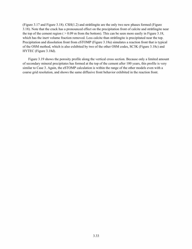
3.33
(Figure 3.17 and Figure 3.18). CSH(1.2) and strätlingite are the only two new phases formed (Figure 3.18). Note that the crack has a pronounced effect on the precipitation front of calcite and strätlingite near the top of the cement region ( > 0.09 m from the bottom). This can be seen more easily in Figure 3.18, which has the inert volume fraction removed. Less calcite than strätlingite is precipitated near the top. Precipitation and dissolution front from eSTOMP (Figure 3.18a) simulates a reaction front that is typical of the OSM method, which is also exhibited by two of the other OSM codes, SC3K (Figure 3.18c) and HYTEC (Figure 3.18d).
Figure 3.19 shows the porosity profile along the vertical cross section. Because only a limited amount of secondary mineral precipitates has formed at the top of the cement after 100 years, this profile is very similar to Case 3. Again, the eSTOMP calculation is within the range of the other models even with a coarse grid resolution, and shows the same diffusive front behavior exhibited in the reaction front.
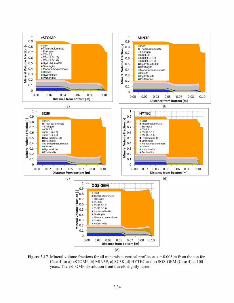
3.34
(a) (b)
(c) (d)
(e)
Figure 3.17. Mineral volume fractions for all minerals at vertical profiles at x = 0.005 m from the top for Case 4 for a) eSTOMP, b) MIN3P, c) SC3K, d) HYTEC and e) SGS-GEM (Case 4) at 100 years. The eSTOMP dissolution front travels slightly faster.
0
0.1
0.2
0.3
0.4
0.5
0.6
0.7
0.8
0.9
1
0.00 0.02 0.04 0.06 0.08 0.10
Mineral V
olume Fraction [‐]
Distance from bottom [m]
InertTricarboaluminateEttringiteCSH0.8CSH(1.0-1.2)CSH(1.3-1.6)Hydrotalcite-OHStratingiteMonocarboaluminateCalciteHydrotalcitePortlandite
eSTOMP
0
0.1
0.2
0.3
0.4
0.5
0.6
0.7
0.8
0.9
1
0.00 0.02 0.03 0.05 0.07 0.08 0.10
Mineral V
olume Fraction [‐]
Distance from bottom [m]
InertTricarboaluminateEttringiteCSH0.8CSH(1.0-1.2)CSH(1.3-1.6)Hydrotalcite-OHStratingiteMonocarboaluminateCalciteHydrotalcitePortlandite
MIN3P
0
0.1
0.2
0.3
0.4
0.5
0.6
0.7
0.8
0.9
1
0.00 0.02 0.03 0.05 0.07 0.08 0.10
Mineral V
olume Fraction [‐]
Distance from bottom [m]
InertTricarboaluminateEttringiteCSH0.8CSH(1.0‐1.2)CSH(1.3‐1.6)Hydrotalcite‐OHStratingiteMonocarboaluminateCalciteHydrotalcitePortlandite
SC3K
0
0.1
0.2
0.3
0.4
0.5
0.6
0.7
0.8
0.9
1
0.00 0.02 0.03 0.05 0.06 0.08 0.10
Mineral V
olume Fraction [‐]
Distance from bottom [m]
InertTricarboaluminateEttringiteCSH0.8CSH(1.0‐1.2)CSH(1.3‐1.6)Hydrotalcite‐OHStratingiteMonocarboaluminateCalciteHydrotalcitePortlandite
HYTEC
0
0.1
0.2
0.3
0.4
0.5
0.6
0.7
0.8
0.9
1
0.00 0.02 0.03 0.05 0.07 0.08 0.10
Mineral V
olume Fraction [‐]
Distance from bottom [m]
InertTricarboaluminateEttringiteCSH0.8CSH(1.0‐1.2)CSH(1.3‐1.6)Hydrotalcite‐OHStratingiteMonocarboaluminateCalciteHydrotalcite
OGS‐GEM
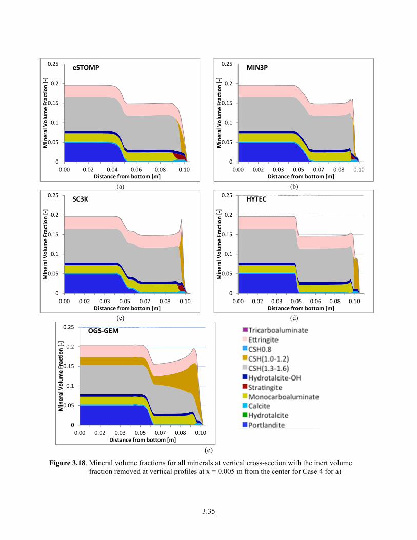
3.35
(a) (b)
(c) (d)
(e)
Figure 3.18. Mineral volume fractions for all minerals at vertical cross-section with the inert volume fraction removed at vertical profiles at x = 0.005 m from the center for Case 4 for a)
0
0.05
0.1
0.15
0.2
0.25
0.00 0.02 0.04 0.06 0.08 0.10
Mineral V
olume Fraction [‐]
Distance from bottom [m]
eSTOMP
0
0.05
0.1
0.15
0.2
0.25
0.00 0.02 0.03 0.05 0.07 0.08 0.10
Mineral V
olume Fraction [‐]
Distance from bottom [m]
MIN3P
0
0.05
0.1
0.15
0.2
0.25
0.00 0.02 0.03 0.05 0.07 0.08 0.10
Mineral V
olume Fraction [‐]
Distance from bottom [m]
SC3K
0
0.05
0.1
0.15
0.2
0.25
0.00 0.02 0.03 0.05 0.06 0.08 0.10
Mineral V
olume Fraction [‐]
Distance from bottom [m]
HYTEC
0
0.05
0.1
0.15
0.2
0.25
0.00 0.02 0.03 0.05 0.07 0.08 0.10
Mineral V
olume Fraction [‐]
Distance from bottom [m]
OGS‐GEM
3.36
eSTOMP, b) MIN3P, c) SC3K, d) HYTEC and e) OGS-GEM (Case 4) at 100 years. The eSTOMP dissolution front travels slightly faster.
Figure 3.19. Porosity profile along the vertical profiles at x = 0.005 m from the center for Case 4.
3.8 Discussion
The goal of the simulations described in this section of the report was to compare simulation results from eSTOMP to those results published in Perko et al. (2015), and to verify the eSTOMP simulator for simulating flow and reactive transport for cementitious waste forms (HCP). All of the simulations included a crack within the cement, with contrasting physical and transport properties. The crack caused localized effects and influenced the leaching process and degradation fronts.
eSTOMP showed a difference in the influence of the crack in Case 2 due to the influence of its kinetic formulation for aqueous-solid phase reactions. For consistency, eSTOMP used the same quasi-equilibrium approach adopted by MIN3P, but still exhibited a slower rate of portlandite dissolution. The kinetic formulation permitted it to be the only simulator that demonstrated the impact of the crack relative to the rest of the domain.
Perko et al. (2015) concluded that differences in simulators were due to differences in solution methods and numerical model formulations. None of the simulators in the benchmark publication was formulated in the same way. eSTOMP is also unique in its approach and formulation. In terms of solution methods, eSTOMP is similar to HYTEC and MIN3P in simulating flow and hydrologic transport. They are all based on the finite volume approach, but they differ in their coupling of hydrologic transport and chemistry. eSTOMP uses non-iterative operator splitting. HYTEC uses a sequential iterative operator-splitting method for coupling between chemistry and transport. The MIN3P code uses a direct substitution approach and the GIM for solving the model equations. SC3K and OGS-GEM are similar to eSTOMP in terms of the OSM used for solving transport and reactions, but they use finite elements to compute flow and transport. All of the codes used equilibrium formulations for describing aqueous mineral reactions, whereas eSTOMP and MIN3P treat these reactions as kinetic, and had to adopt a quasi-equilibrium approach to represent the mineral reactions.
0
0.1
0.2
0.3
0.4
0 0.02 0.04 0.06 0.08 0.1
Porosity
Distance from bottom (m)
eSTOMP MIN3P
SC3K OGS‐GEM
HYTEC
3.37
The non-reactive tracer agreement is excellent among all of the models. However, the largest differences among the codes were observed when mineral reactions were involved. Several possible causes were cited in Perko et al. (2015) and included the following: 1) spatial weighting of properties differs among the codes (e.g., for FEM, concentrations are computed on the nodes, but porosity is computed for the element, whereas for FVM all calculations occur on the nodes); 2) finite volume is a locally mass conservative method while finite element is globally mass conservative; 3) sequential non-iterative coupling causes numerical error; and 4) the cumulative impact of all of these differences over a large number of iterations led to small discrepancies between models. However, eSTOMP was demonstrated to be robust and provided similar results to the other codes.
4.1
4.0 Discussion and Summary
The goal of the work described in this report was to provide confidence to the extent possible in the use of the eSTOMP simulator. However, there were several challenges associated with demonstrating this successfully, since comparisons to other simulators were complicated by different conceptual and numerical formulations, and comparisons to data were obfuscated by data quality.
The eSTOMP benchmarking was challenged by differences in model formulations. The simulators participating in the benchmark simulations experienced this same challenge, as evidenced by the incomplete participation of all of the simulators in each of the benchmark cases. Modifications to the reported inputs were also identified, which underscores how small differences in numerical approaches may warrant adjustments to input data to match the desired outputs. This also emphasizes the importance of calibration for any application, especially with the knowledge of how numerical methods can influence the solution. Differences among the codes are expected given differences in approaches. These included the representation of solid and aqueous phase reactions, numerical formulation (FVM vs. FEM), and the coupling of reactions and transport. Because transport affects reaction-coupled systems, such differences can affect the final solution.
In the eSTOMP glass simulations, problems with the manufacture of the glass meant that the parameters initially identified for glass degradation did not apply to the glass used in the lysimeter experiments. As stated by Pierce et al. (2013), the B and Mo effluent concentrations represented an accelerated LAWA44 glass release rate. To account for the accelerated release in the lysimeter simulations, the CO2 gas concentrations were not fixed, which permitted a faster dissolution rate. Also contributing to a faster rate was the assumption that the reactive surface area was not influenced by water content. Although these two assumptions were not used in the 2005 ILAW PA calculations, the glass used in the lysimeter was not the same as the glass modeled in the PA. Elimination of these assumptions produced a reasonable match between simulated and observed data, which again underscores the need for model calibration.
The eSTOMP simulator is a parallel code, and therefore can simulate both laboratory and field-scale applications. For 3D efficiency, it has adopted an operator-split approach to transport and reactions, where transport and geochemical reaction solutions are computed in separate sub-steps. This contrasts with the global implicit approach, which, because it solves both transport and reactions simultaneously, is generally computationally limited to 1D and 2D simulations. Operator splitting methods typically generate a numerical widening of reaction fronts relative to the global implicit approach. Time steps must be kept small to reduce the splitting error. Because eSTOMP does not iterate between transport and reactions to a convergent solution, the time step constraint is strict, but presumably executes faster relative to an approach that iterates between the transport and reaction equations.
In a discussion of earth model verification and validation, Oreskes et al. (1994) defined the word verify as an assertion or establishment of truth. Thus, a literal interpretation is that the truth of a simulator has been demonstrated. Demonstrating model veracity, however, is a daunting task because of the complications presented by incomplete data sets and numerical formulations. Although it is recognized that this assessment is somewhat subjective, the simulations presented within this report demonstrate that eSTOMP can simulate the degradation of both glass and cementitious waste forms to be emplaced within

4.2
the IDF repository. These results provide confidence that eSTOMP can produce physically realistic simulation results for waste degradation and contaminant transport in support of the IDF PA.
5.1
5.0 References
Archie GE. 1942. “Electrical Resistivity Log as an Aid in Determining Some Reservoir Characteristics.” Trans. AIME 146:54–61.
ASME NQA-1-2000, Quality Assurance Requirements for Nuclear Facility Applications. American Society of Mechanical Engineers, New York.
ASME NQA-1-2008, Quality Assurance Requirements for Nuclear Facility Applications. American Society of Mechanical Engineers, New York.
ASME NQA-1a-2009, Addenda to ASME NQA-1-2008 Quality Assurance Requirements for Nuclear Facility Applications. American Society of Mechanical Engineers, New York.
ASTM Standard C29-85. 1985. Standard Test Method for Bulk Density (Unit Weight) and Voids in Aggregate. ASTM International, West Conshohocken, PA. doi:10.1520/C0033-03, www.astm.org.
Bacon DH and BP McGrail. 2005. Waste Form Release Calculations for the 2005 Integrated Disposal Facility Performance Assessment. PNNL-15198, Pacific Northwest National Laboratory, Richland, WA.
Bacon DH, MD White and BP McGrail. 2005. Subsurface Transport Over Reactive Multiphases (STORM): A Parallel, Coupled, Nonisothermal Multiphase Flow, Reactive Transport, and Porous Medium Alteration Simulator, Version 3.0 . PNNL-14783, Pacific Northwest National Laboratory, Richland, WA.
Bacon, DH and BP McGrail. 2001. Waste Form Release Calculations for the 2001 Immobilized Low- Activity Waste Performance Assessment. PNNL-13369, Pacific Northwest National Laboratory, Richland, WA.
Bacon DH, MD White, and BP McGrail. 2000. Subsurface Transport Over Reactive Multiphases (STORM): A General, Coupled, Nonisothermal Multiphase Flow, Reactive Transport, and Porous Medium Alteration Simulator, Version 2, User's Guide. Pacific Northwest National Laboratory, Richland, WA.
Cantrell KJ. 2014. Geochemical Modeling of ILAW Lysimeter Water Extracts. PNNL-23693, Pacific Northwest National Laboratory, Richland, WA.
COMSOL. 2008. COMSOL Multiphysics: User’s Guide. COMSOL, Inc., Burlington, MA.
Davis PA, NE Olague, and MT Goodrich. 1991. Approaches for the validation of models usedJor performance assessment of high-level nuclear waste repositories. SAND90-0575, Sandia National Laboratories, Albuquerque, NM.
de Marsily G, P Combes, and P Goblet P. 1992. “Comment on groundwater models cannot be validated, by L.F. Konikow and J.D. Bredehoeft.” Water Resour. Res. 15:367–9.
5.2
DOE. 1986. Environmental assessment-- Yucca Mountain site, Nevada Research and Development Area, Nevada. DOE/RW-0073, Vol. 2, U.S. Department of Energy, Office of Civilian Radioactive Waste Management,Washington, DC.
Fang, Y, D Appriou, D Bacon, V Freedman, M Rockhold, C Ruprecht, G Tartakovsky, M White, S White, and F Zhang. 2015. STOMP User Guide. Pacific Northwest National Laboratory. http://stomp.pnnl.gov/estomp_guide/eSTOMP_guide.stm
Gaines GL and HC Thomas. 1953. “Adsorption studies on clay minerals. II. A formulation of the thermodynamics of exchange adsorption..” Journal of Chemical Physics. 21:714-718.
Gee GW and JW Bauder. 1986. “Particle-size analysis.” p. 383–411. In A Klute (ed.) Methods of soil analysis. Part 1. 2nd ed. Agron.Monogr. 9. ASA and SSSA, Madison, WI.
Grathwohl P. 1998. Diffusion in Natural Porous Media: Contaminent Transport, Sorption/Desorption and Dissolution Kinetics. Kluwer Academic Publishers, Norwell, MA.
Hammond, GE and PC Lichtner. 2010. “Field-scale model for the natural attenuation of uranium at the Hanford 300 Area using high-performance computing. Water Resourc. Res. 46(9):W09527.
Horton DG, HT Schaef, RJ Serne, CF Brown, MM Valenta, TS Vickerman, IV Kutnyakov, SR Baum, KN Geiszler, and KE Parker. 2003. Geochemistry of Samples from Borehole C3177(299-E24-21). PNNL-14289, Pacific Northwest National Laboratory, Richland, WA.
Jacques D, L Wang, E Martens, and D Mallants. 2010. “Modelling chemical degradation of concrete during leaching with rain and soil water types.” Cem. Concr. Res. 40 1306–1313.
Jardine, PM and DL.Sparks. 1984. “Potassium-calcium exchange in a multi-reactive soil system.” Soil Sci. Soc. Am. J. 47:39-50.
Kini KA, RM Manser, and AS Joy. 1968. “Surface Area of Silicate Minerals by Bet Method Using Adsorption of Xenon at -78 Degrees.” Journal of Physical Chemistry 72(6):2127-2129 doi:10.1021/j100852a042
Klute A and C Dirksen. 1986. “Hydraulic conductivity anddiffusivity: laboratory methods.” In A Klute (ed.), Methods of Soil Analysis. Part 1. Physical and Mineralogical Methods, 2nd ed. Agron. Monogr. 9. ASA, Madison, WI, pp. 687–734.
Klute A. 1986. “Water retention: Laboratory methods.” p. 597–618. In A Klute (ed.) Methods of soil analysis. Part 1. 2nd ed. Agron. Monogr. 9. ASA and SSSA, Madison, WI.
Kulik DA, T Wagner, SV Dmytrieva, G Kosakowski, FF Hingerl, KV Chudnenko, and U Berner. 2013. “GEM-Selektor geochemical modeling package: Numerical kernel GEMS3K for coupled simulation codes.” Comput. Geosci. 17:1–24.
Konikow, LF, and JD Bredehoeft. 1992. “Ground-water models cannot be validated.” Advances in Water Resources. 15(1):75-83.
5.3
Last G, M Snyder, W Um, J Stephenson, I Leavy, C Strickland, D Bacon, N Qafoku, and R Serne. 2015. Technetium, Iodine, and Chromium Adsorption/Desorption Kd Values for Vadose Zone Pore Water, ILAW Glass, and Cast Stone Leachates Contacting an IDF Sand Sequence. PNNL-24683, Pacific Northwest National Laboratory, Richland, Washington. Laudelout H, R van Bladel, GH Bolt, AL Page. 1968. Thermodynamics of heterovalent cation exchange reactions in a montmorillonite clay. Trans. Faraday Soc. 64:1477-1488.
Liu, CW and TN Narasimhan. 1989. “Redox-controlled multiple-species reactive chemical transport 2. Verification and application.” Water Resour. Res. 25(5):869-882.
Mann, FM, Burgard, KC, Root, WR, Puigh, RP, Finfrock, SH, Khaleel, R, Bacon, DH, Freeman, EJ, McGrail, BP, Wurstner, SK, LaMont, PE. 2001. Hanford Immobilization Low-Activity Tank Waste Performance Assessment: 2001 Version. DOE/ORP-2000-24, US Department of Energy, Office of River Protection, Richland, WA.
Matalas, NC, JM Landwehr, and MG Wolman. 1982. “Prediction in water management.” In Scientific basis of water resource management. National Research Council, National Academy Press, Washington, DC.
Mayer, KU. 2015. Electronic mail communication to Yilin Fang (Pacific Northwest National Laboratory) from Uli Mayer (University of British Columbia). “Mineral Rate Expression.” December 16, 2015. Copy of data has been archived in ILAW Project Records for Report No. RPT-IGTP-010.
Mayer KU, EO Frind, and DW Blowes. 2002. “Multicomponent reactive transport modeling in variably saturated porous media using a generalized formulation for kinetically controlled reactions.” Water Resour. Res. 38.
McGrail BP. 2001. "Inverse Reactive Transport Simulator (Inverts): An Inverse Model for Contaminant Transport with Nonlinear Adsorption and Source Terms." Environmental Modelling & Software, with Environmental Data News 16(8):711-723.
Meeussen, JCL. 2003. “ORCHESTRA: An object-oriented framework for implementing chemical equilibrium models.” Environ Sci. Technol. 37:1175–1182.
Meyer, PD. 2015. Electronic mail communication to Diana Bacon (Pacific Northwest National Laboratory) from Philip Meyer (Pacific Northwest National Laboratory). “Lysimeter Data.” April 10, 2015. Copy of data has been archived in ILAW Project Records for Report No. RPT-IGTP-010.
Meyer, PD. 2015. Electronic mail communication to Diana Bacon (Pacific Northwest National Laboratory) from Philip Meyer (Pacific Northwest National Laboratory). “Lysimeter Data.” April 10, 2015. Copy of data has been archived in ILAW Project Records for Report No. RPT-IGTP-010.
Meyer PD, BP McGrail, and DH Bacon. 2001. Test Plan for Field Experiments to Support the Immobilized Low-Activity Waste Disposal Performance Assessment at the Hanford Site. PNNL-13670, Pacific Northwest National Laboratory, Richland, WA.
5.4
Meyer PD, KP Saripalli, and VL Freedman. 2004. Near-Field Hydrology Data Package for the Integrated Disposal Facility 2005 Performance Assessment. PNNL-14700, Pacific Northwest National Laboratory, Richland, WA. http://dx.doi.org/10.2172/15010637.
Mualem, Y. 1976. “A new model for predicting the hydraulic conductivity of unsaturated porous media.” Water Resourc. Res., 12: 513-522.
NRC. 1986. A revised modelling strategy document for high-level waste performance assessment. U.S. Nuclear Regulatory Commission, Washington, DC.
Oreskes N, K Shrader-Frechette K, and K Belitz. 1994. “Verification, validation and confirmation of numerical models in the earth sciences.” Science 263:641–6.
Palandri JL and YK Kharaka. 2004. A Compilation of Rate Parameters of Water-Mineral Interaction Kinetics for Application to Geochemical Modeling. Open File Report 2004-1068, U.S. Geological Survey, Menlo Park, California. http://pubs.usgs.gov/of/2004/1068/.
Parkhurst DL and CAJ Appello. 1999. “User’s guide to PHREEQC (version 2)—a computer program for speciation, reactionpath, 1D-transport, and inverse geochemical calculations.” US Geol. Surv. Water Resour. Inv. Rep. 312:99–4259 .
Perko J, KU Mayer, G Koskowski, L De Windt, J Govaerts, D Jacques, D Su, and JCL Meeussen. 2015. “Decalcification of cracked cement structures.” Computational Geosciences. doi:10.1007/s10596-014-9467-2
Pierce EM, BP McGrail, EA Rodriguez, HT Schaef, P Saripalli, RJ Serne, KM Krupka, PF Martin, SR Baum, KN Geiszler, LR Reed, and WJ Shaw. 2004. Waste Form Release Data Package for the 2005 Integrated Disposal Facility Performance Assessment. PNNL-14805, Pacific Northwest National Laboratory, Richland, WA. http://dx.doi.org/10.2172/15020942.
Pierce EM, SN Kerisit, EJ Krogstad, SD Burton, BN Bjornstad, VL Freedman, KJ Cantrell, MM Valenta, JV Crum, and JH Westsik. 2013. Integrated Disposal Facility FY 2012 Glass Testing Summary Report. PNNL-21812, Rev. 1, Pacific Northwest National Laboratory, Richland, WA.
Popper K. 1959. The Logic of Scientific Discovery. Harper and Row, New York.
Refsgaard JC. 1997. “Parameterisation, calibration and validation of distributed hydrological models.” Journal of Hydrology 198:69-97.
Rimstidt JD and HL Barnes. 1980. “The kinetics of silica-water reactions.” Geochim. et Cosmochim. Acta 44:1683-1699.
Schlesinger, S. 1979. “Terminology for model credibility.” Simulation. 32(3):103-104.
Serne, J. 2015. Electronic mail communication to Diana Bacon (Pacific Northwest National Laboratory) from Kirk Cantrell (Pacific Northwest National Laboratory), forwarding data that originated from Jeff Serne (Pacific Northwest National Laboratory). “Glass with Ion Exchange.” October 21, 2014. Copy of data has been archived in ILAW Project Records for Report No. RPT-IGTP-010.
5.5
Sø HU, D Postma, R Jakobsen, and F Larsen. 2011. “Sorption of phosphate onto calcite; results from batch experiments and surface complexation modeling.” Geochimica et Cosmochimica Acta 75(10):2911-2923. http://dx.doi.org/10.1016/j.gca.2011.02.031.
Steefel CI and KTB MacQuarrie. 1996. “Approaches to modeling of reactive transport in porous media.” In PC Lichtner, CI Steefel, EH Oelkers (eds.), Reviews in mineralogy, vol. 34. Mineralogical Society of America, Washington, DC, pp. 83–129 [chapter 2].
Steefel CI, SB Yabusaki, and Y Fang. 2015. "Reactive transport benchmarks for subsurface environmental simulation." Computational Geosciences. doi:10.1007/s10596-015-9499-2.
Strachan, D. 2009. Letter report on Re releases in the lysimeter tests. Pacific Northwest National Laboratory. Sent to Ms. Kris Colosi on January 14, 2009.
Van Bladel, R and HR Gheyi. 1980. “Thermodynamic study of calcium-sodium and calcium-magnesium exchange in calcareous soils.” Soil Sci. Soc. Am. J. 44:938–942.
van der Lee J, L De Windt, V Lagneau, and P Goblet. 2003. “Module oriented modeling of reactive transport with HYTEC.” Comput. Geosci. 29:265–275.
van Genuchten, MTh. 1980. “A closed-form equation for predicting the hydraulic conductivity of unsaturated soils.” Soil Sci. Soc. Am. J. 44: 892–898.
White M, D Appriou, D Bacon, Y Fang, V Freedman, M Rockhold, C Ruprecht, G Tartakovsky, S White, and F Zhang. 2015. STOMP User Guide. Pacific Northwest National Laboratory. http://stomp.pnnl.gov/user_guide/STOMP_guide.stm.
White MD and M Oostrom. 2000. STOMP Subsurface Transport Over Multiple Phases Version 2.0 Theory Guide. PNNL-12030, Pacific Northwest National Laboratory, Richland, WA.
Wicks GG. 2001. “US field testing programs and results.” Journal of Nuclear Materials 298(1): 78-85.
Yabusaki, S. 2015. Electronic mail communication to Yilin Fang (Pacific Northwest National Laboratory) from Steven Yabusaki (Pacific Northwest National Laboratory). “Perko et al. 2015 Benchmark Inputs and Outputs.” January 14, 2015. Copy of data has been archived in ILAW Project Records for Report No. RPT-IGTP-010.
Yeh GT and VS Tripathi. 1989. “A critical evaluation of recent developments in hydrogeochemical transport models of reactive multichemical components. Water Resour. Res. 25(1):93-108.
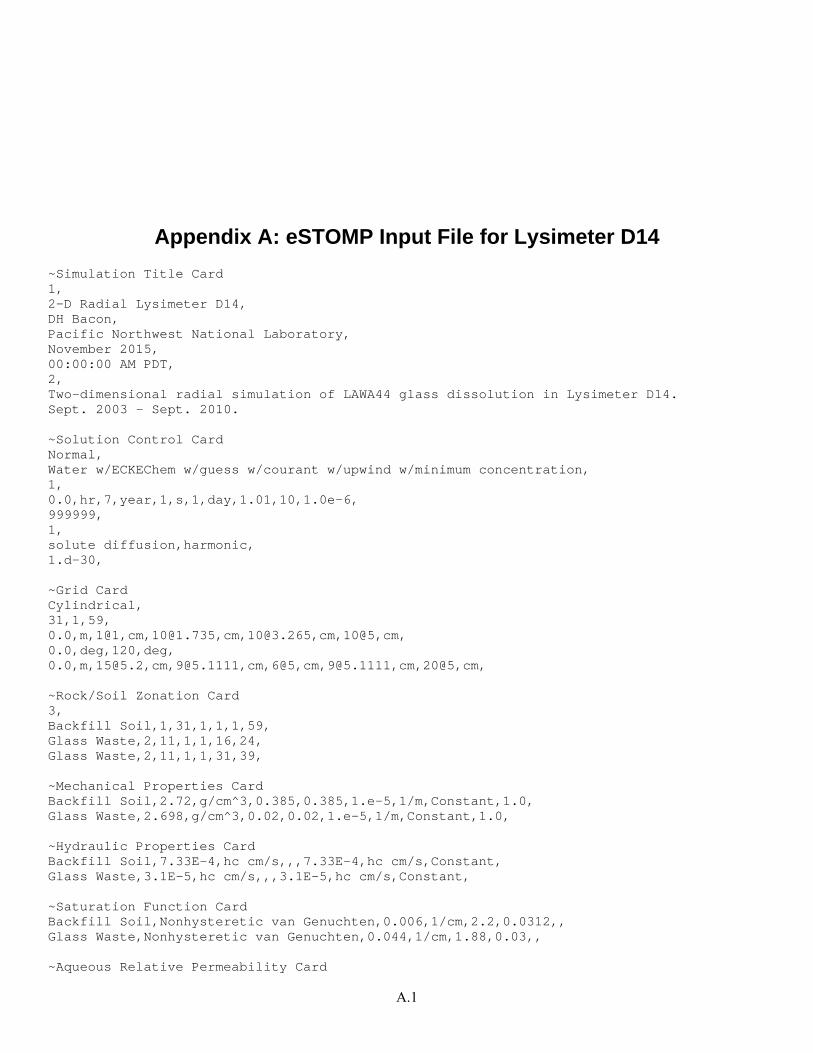
A.1
Appendix A: eSTOMP Input File for Lysimeter D14 ~Simulation Title Card 1, 2-D Radial Lysimeter D14, DH Bacon, Pacific Northwest National Laboratory, November 2015, 00:00:00 AM PDT, 2, Two-dimensional radial simulation of LAWA44 glass dissolution in Lysimeter D14. Sept. 2003 - Sept. 2010. ~Solution Control Card Normal, Water w/ECKEChem w/guess w/courant w/upwind w/minimum concentration, 1, 0.0,hr,7,year,1,s,1,day,1.01,10,1.0e-6, 999999, 1, solute diffusion,harmonic, 1.d-30, ~Grid Card Cylindrical, 31,1,59, 0.0,m,1@1,cm,[email protected],cm,[email protected],cm,10@5,cm, 0.0,deg,120,deg, 0.0,m,[email protected],cm,[email protected],cm,6@5,cm,[email protected],cm,20@5,cm, ~Rock/Soil Zonation Card 3, Backfill Soil,1,31,1,1,1,59, Glass Waste,2,11,1,1,16,24, Glass Waste,2,11,1,1,31,39, ~Mechanical Properties Card Backfill Soil,2.72,g/cm^3,0.385,0.385,1.e-5,1/m,Constant,1.0, Glass Waste,2.698,g/cm^3,0.02,0.02,1.e-5,1/m,Constant,1.0, ~Hydraulic Properties Card Backfill Soil,7.33E-4,hc cm/s,,,7.33E-4,hc cm/s,Constant, Glass Waste,3.1E-5,hc cm/s,,,3.1E-5,hc cm/s,Constant, ~Saturation Function Card Backfill Soil,Nonhysteretic van Genuchten,0.006,1/cm,2.2,0.0312,, Glass Waste,Nonhysteretic van Genuchten,0.044,1/cm,1.88,0.03,, ~Aqueous Relative Permeability Card
A.2
Backfill Soil,Mualem,, Glass Waste,Mualem,, ~Gas Relative Permeability Card Backfill Soil,Mualem,, Glass Waste,Mualem,, ~Solute/Porous Media Interaction Card Backfill Soil,0.01,m,0.0,m, Glass Waste,0.01,m,0.0,m, ~Aqueous Species Card 57,Power,1.84e-5,cm^2/s,1.486,1.956,Bdot,1.0, Al+++, 3.0, 9.0,A, 26.9815,kg/kmol, AlO2-, -1.0, 4.0,A, 58.9803,kg/kmol, B(OH)3(aq), 0.0, 3.0,A, 61.8330,kg/kmol, BO2-, -1.0, 4.0,A, 42.8098,kg/kmol, CO2(aq), 0.0, 3.0,A, 44.0098,kg/kmol, CO3--, -2.0, 4.5,A, 60.0092,kg/kmol, Ca++, 2.0, 6.0,A, 40.0780,kg/kmol, CaCO3(aq), 0.0, 3.0,A, 100.0872,kg/kmol, CaCl+, 1.0, 4.0,A, 75.5307,kg/kmol, CaF+, 1.0, 4.0,A, 59.0764,kg/kmol, CaHCO3+, 1.0, 4.0,A, 101.0951,kg/kmol, CaSO4(aq), 0.0, 3.0,A, 136.1416,kg/kmol, Cl-, -1.0, 3.0,A, 35.4527,kg/kmol, CrO4--, -2.0, 4.0,A, 115.9937,kg/kmol, F-, -1.0, 3.5,A, 18.9984,kg/kmol, Fe(OH)3(aq), 0.0, 3.0,A, 106.8690,kg/kmol, Fe+++, 3.0, 9.0,A, 55.8470,kg/kmol, H+, 1.0, 9.0,A, 1.0079,kg/kmol, H2PO4-, -1.0, 4.0,A, 96.9872,kg/kmol, HCO3-, -1.0, 4.0,A, 61.0171,kg/kmol, HCrO4-, -1.0, 4.0,A, 117.0016,kg/kmol, HPO4--, -2.0, 4.0,A, 95.9793,kg/kmol, HSiO3-, -1.0, 4.0,A, 77.0916,kg/kmol, I-, -1.0, 3.0,A, 126.9045,kg/kmol, K+, 1.0, 3.0,A, 39.0983,kg/kmol, KCl(aq), 0.0, 3.0,A, 74.5510,kg/kmol, KSO4-, -1.0, 4.0,A, 135.1619,kg/kmol, Mg++, 2.0, 8.0,A, 24.3050,kg/kmol, MgCO3(aq), 0.0, 3.0,A, 84.3142,kg/kmol, MgCl+, 1.0, 4.0,A, 59.7577,kg/kmol, MgF+, 1.0, 4.0,A, 43.3034,kg/kmol, MgHCO3+, 1.0, 4.0,A, 85.3221,kg/kmol, MgP2O7--, -2.0, 4.0,A, 198.2483,kg/kmol, MgSO4(aq), 0.0, 3.0,A, 120.3686,kg/kmol, MoO4--, -2.0, 4.5,A, 159.9376,kg/kmol, NO3-, -1.0, 3.0,A, 62.0049,kg/kmol, Na+, 1.0, 4.0,A, 22.9898,kg/kmol, NaAlO2(aq), 0.0, 3.0,A, 81.9701,kg/kmol, NaCO3-, -1.0, 4.0,A, 82.9990,kg/kmol, NaCl(aq), 0.0, 3.0,A, 58.4425,kg/kmol, NaF(aq), 0.0, 3.0,A, 41.9882,kg/kmol, NaHCO3(aq), 0.0, 3.0,A, 84.0069,kg/kmol, NaHSiO3(aq), 0.0, 3.0,A, 100.0814,kg/kmol, NaOH(aq), 0.0, 3.0,A, 39.9971,kg/kmol, OH-, -1.0, 3.5,A, 17.0073,kg/kmol, PO4---, -3.0, 4.0,A, 94.9714,kg/kmol, ReO4-, -1.0, 4.0,A, 250.2046,kg/kmol, SO4--, -2.0, 4.0,A, 96.0636,kg/kmol,
A.3
SeO3--, -2.0, 4.0,A, 126.9582,kg/kmol, SiO2(aq), 0.0, 3.0,A, 60.0843,kg/kmol, Ti(OH)4(aq), 0.0, 3.0,A, 115.9094,kg/kmol, Zn++, 2.0, 6.0,A, 65.3900,kg/kmol, ZnCl+, 1.0, 4.0,A, 100.8427,kg/kmol, ZnCl2(aq), 0.0, 3.0,A, 136.2954,kg/kmol, ZnSO4(aq), 0.0, 3.0,A, 161.4536,kg/kmol, Zr(OH)2++, 2.0, 4.5,A, 125.2387,kg/kmol, Zr(OH)4(aq), 0.0, 3.0,A, 159.2534,kg/kmol, ~Solid Species Card 17, Albite_high, 2.611,g/cm^3, 262.2230,kg/kmol, Analcime, 2.265,g/cm^3, 219.2786,kg/kmol, Anatase, 3.900,g/cm^3, 79.8788,kg/kmol, Baddeleyite, 5.750,g/cm^3, 123.2228,kg/kmol, Calcite, 2.710,g/cm^3, 100.0872,kg/kmol, Chalcedony, 2.648,g/cm^3, 60.0843,kg/kmol, Clinochlore-14A, 2.684,g/cm^3, 555.7973,kg/kmol, Fe(OH)3, 3.110,g/cm^3, 106.8690,kg/kmol, Gibbsite, 2.441,g/cm^3, 78.0036,kg/kmol, K-Feldspar, 2.557,g/cm^3, 278.3315,kg/kmol, LAWA44, 2.698,g/cm^3, 67.0600,kg/kmol, LAWA44-H, 2.315,g/cm^3, 57.5500,kg/kmol, Muscovite, 2.831,g/cm^3, 398.3081,kg/kmol, Quartz, 2.648,g/cm^3, 60.0843,kg/kmol, Sepiolite, 2.268,g/cm^3, 647.8304,kg/kmol, Tremolite, 2.977,g/cm^3, 812.3665,kg/kmol, Zn(OH)2(gamma), 3.330,g/cm^3, 99.4047,kg/kmol, ~Exchanged Species Card 4, 1,Gaines-Thomas, CaX2,Ca++,1, KX,K+,1, MgX2,Mg++,1, NaX,Na+,1, ~Conservation Equations Card 24, Total_AlO2-, 11,Al+++, 1.0000E+00,AlO2-, 1.0000E+00,Albite_high, 1.0000E+00,Analcime, 9.6000E-01,Clinochlore-14A, 2.0000E+00,Gibbsite, 1.0000E+00,K-Feldspar, 1.0000E+00,LAWA44, 8.1712E-02,LAWA44-H, 8.1712E-02,Muscovite, 3.0000E+00,NaAlO2(aq), 1.0000E+00, Total_B(OH)3(aq), 4,B(OH)3(aq), 1.0000E+00,BO2-, 1.0000E+00,LAWA44, 1.7179E-01,LAWA44-H, 1.7179E-01, Total_Ca++, 11,Ca++, 1.0000E+00,CaCO3(aq), 1.0000E+00,CaCl+, 1.0000E+00,CaF+, 1.0000E+00,CaHCO3+, 1.0000E+00,CaSO4(aq), 1.0000E+00,CaX2, 1.0000E+00,Calcite, 1.0000E+00,LAWA44, 2.3842E-02,LAWA44-H, 2.3842E-02,Tremolite, 2.0000E+00, Total_Cl-, 9,CaCl+, 1.0000E+00,Cl-, 1.0000E+00,KCl(aq), 1.0000E+00,LAWA44, 1.2319E-02,LAWA44-H, 1.2319E-02,MgCl+, 1.0000E+00,NaCl(aq), 1.0000E+00,ZnCl+, 1.0000E+00,ZnCl2(aq), 2.0000E+00, Total_CrO4--, 4,CrO4--, 1.0000E+00,HCrO4-, 1.0000E+00,LAWA44, 1.7683E-04,LAWA44-H, 1.7683E-04, Total_F-, 6,CaF+, 1.0000E+00,F-, 1.0000E+00,LAWA44, 3.5366E-04,LAWA44-H, 3.5366E-04,MgF+, 1.0000E+00,NaF(aq), 1.0000E+00, Total_Fe(OH)3(aq), 5,Fe(OH)3, 1.0000E+00,Fe(OH)3(aq), 1.0000E+00,Fe+++, 1.0000E+00,LAWA44, 5.8736E-02,LAWA44-H, 5.8736E-02, Total_H+, 26,Al+++, 4.0000E+00,BO2-,-1.0000E+00,CO2(aq), 1.0000E+00,CO3--,-1.0000E+00,CaCO3(aq),-1.0000E+00,Calcite,-1.0000E+00,Clinochlore-14A,-8.0000E+00,Fe+++, 3.0000E+00,Gibbsite, 1.0000E+00,H+, 1.0000E+00,H2PO4-, 1.0000E+00,HCrO4-, 1.0000E+00,
A.4
HSiO3-,-1.0000E+00,LAWA44,-5.4914E-01,LAWA44-H,-1.1551E-01,MgCO3(aq),-1.0000E+00,Muscovite, 2.0000E+00,NaCO3-,-1.0000E+00,NaHSiO3(aq),-1.0000E+00,NaOH(aq),-1.0000E+00,OH-,-1.0000E+00,PO4---,-1.0000E+00,Sepiolite,-8.0000E+00,Tremolite,-1.4000E+01, Zn(OH)2(gamma),-2.0000E+00,Zr(OH)2++, 2.0000E+00, Total_HCO3-, 10,CO2(aq), 1.0000E+00,CO3--, 1.0000E+00,CaCO3(aq), 1.0000E+00,CaHCO3+, 1.0000E+00,Calcite, 1.0000E+00,HCO3-, 1.0000E+00,MgCO3(aq), 1.0000E+00,MgHCO3+, 1.0000E+00,NaCO3-, 1.0000E+00,NaHCO3(aq), 1.0000E+00, Total_HPO4--, 6,H2PO4-, 1.0000E+00,HPO4--, 1.0000E+00,LAWA44, 2.8401E-04,LAWA44-H, 2.8401E-04,MgP2O7--, 2.0000E+00,PO4---, 1.0000E+00, Total_I-, 3,I-, 1.0000E+00,LAWA44, 5.2945E-04,LAWA44-H, 5.2945E-04, Total_K+, 8,K+, 1.0000E+00,K-Feldspar, 1.0000E+00,KCl(aq), 1.0000E+00,KSO4-, 1.0000E+00,KX, 1.0000E+00,LAWA44, 7.1324E-03,LAWA44-H, 7.1324E-03,Muscovite, 1.0000E+00, Total_Mg++, 13,Clinochlore-14A, 5.0000E+00,LAWA44, 3.3169E-02,LAWA44-H, 3.3169E-02,Mg++, 1.0000E+00,MgCO3(aq), 1.0000E+00,MgCl+, 1.0000E+00,MgF+, 1.0000E+00,MgHCO3+, 1.0000E+00,MgP2O7--, 1.0000E+00,MgSO4(aq), 1.0000E+00,MgX2, 1.0000E+00,Sepiolite, 4.0000E+00,Tremolite, 5.0000E+00, Total_MoO4--, 3,LAWA44, 4.6679E-04,LAWA44-H, 4.6679E-04,MoO4--, 1.0000E+00, Total_NO3-, 1,NO3-, 1.0000E+00, Total_Na+, 14,Albite_high, 1.0000E+00,Analcime, 9.6000E-01,CaX2,-2.0000E+00,KX,-1.0000E+00,LAWA44, 4.3363E-01,MgX2,-2.0000E+00,Na+, 1.0000E+00,NaAlO2(aq), 1.0000E+00,NaCO3-, 1.0000E+00,NaCl(aq), 1.0000E+00,NaF(aq), 1.0000E+00,NaHCO3(aq), 1.0000E+00,NaHSiO3(aq), 1.0000E+00,NaOH(aq), 1.0000E+00, Total_NaX, 4,CaX2, 2.0000E+00,KX, 1.0000E+00,MgX2, 2.0000E+00,NaX, 1.0000E+00, Total_ReO4-, 3,LAWA44, 3.0793E-04,LAWA44-H, 3.0793E-04,ReO4-, 1.0000E+00, Total_SO4--, 7,CaSO4(aq), 1.0000E+00,KSO4-, 1.0000E+00,LAWA44, 8.3922E-04,LAWA44-H, 8.3922E-04,MgSO4(aq), 1.0000E+00,SO4--, 1.0000E+00,ZnSO4(aq), 1.0000E+00, Total_SeO3--, 3,LAWA44, 6.0554E-04,LAWA44-H, 6.0554E-04,SeO3--, 1.0000E+00, Total_SiO2(aq), 14,Albite_high, 3.0000E+00,Analcime, 2.0400E+00,Chalcedony, 1.0000E+00,Clinochlore-14A, 3.0000E+00,HSiO3-, 1.0000E+00,K-Feldspar, 3.0000E+00,LAWA44, 4.9527E-01,LAWA44-H, 4.9527E-01,Muscovite, 3.0000E+00,NaHSiO3(aq), 1.0000E+00,Quartz, 1.0000E+00,Sepiolite, 6.0000E+00,SiO2(aq), 1.0000E+00,Tremolite, 8.0000E+00, Total_Ti(OH)4(aq), 4,Anatase, 1.0000E+00,LAWA44, 1.6735E-02,LAWA44-H, 1.6735E-02,Ti(OH)4(aq), 1.0000E+00, Total_Zn++, 7,LAWA44, 2.4442E-02,LAWA44-H, 2.4442E-02,Zn(OH)2(gamma), 1.0000E+00,Zn++, 1.0000E+00,ZnCl+, 1.0000E+00,ZnCl2(aq), 1.0000E+00,ZnSO4(aq), 1.0000E+00, Total_Zr(OH)4(aq), 5,Baddeleyite, 1.0000E+00,LAWA44, 1.6304E-02,LAWA44-H, 1.6304E-02,Zr(OH)2++, 1.0000E+00,Zr(OH)4(aq), 1.0000E+00, ~Equilibrium Equations Card 37, 3,Al+++,AlO2-, 1.0000,H+, 4.0000,EqRc-1, 1.0000, 3,BO2-,B(OH)3(aq), 1.0000,H+, -1.0000,EqRc-2, 1.0000, 3,CO2(aq),H+, 1.0000,HCO3-, 1.0000,EqRc-3, 1.0000, 3,CO3--,H+, -1.0000,HCO3-, 1.0000,EqRc-4, 1.0000, 4,CaCO3(aq),Ca++, 1.0000,H+, -1.0000,HCO3-, 1.0000,EqRc-5, 1.0000, 3,CaCl+,Ca++, 1.0000,Cl-, 1.0000,EqRc-6, 1.0000, 3,CaF+,Ca++, 1.0000,F-, 1.0000,EqRc-7, 1.0000, 3,CaHCO3+,Ca++, 1.0000,HCO3-, 1.0000,EqRc-8, 1.0000, 3,CaSO4(aq),Ca++, 1.0000,SO4--, 1.0000,EqRc-9, 1.0000, 4,CaX2,Ca++, 1.0000,Na+, -2.0000,NaX, 2.0000,EqRc-10, 1.0000, 3,Fe+++,Fe(OH)3(aq), 1.0000,H+, 3.0000,EqRc-11, 1.0000, 3,H2PO4-,H+, 1.0000,HPO4--, 1.0000,EqRc-12, 1.0000, 3,HCrO4-,CrO4--, 1.0000,H+, 1.0000,EqRc-13, 1.0000, 3,HSiO3-,H+, -1.0000,SiO2(aq), 1.0000,EqRc-14, 1.0000, 3,KCl(aq),Cl-, 1.0000,K+, 1.0000,EqRc-15, 1.0000, 3,KSO4-,K+, 1.0000,SO4--, 1.0000,EqRc-16, 1.0000, 4,KX,K+, 1.0000,Na+, -1.0000,NaX, 1.0000,EqRc-17, 1.0000, 4,MgCO3(aq),H+, -1.0000,HCO3-, 1.0000,Mg++, 1.0000,EqRc-18, 1.0000, 3,MgCl+,Cl-, 1.0000,Mg++, 1.0000,EqRc-19, 1.0000, 3,MgF+,F-, 1.0000,Mg++, 1.0000,EqRc-20, 1.0000,
A.5
3,MgHCO3+,HCO3-, 1.0000,Mg++, 1.0000,EqRc-21, 1.0000, 3,MgP2O7--,HPO4--, 2.0000,Mg++, 1.0000,EqRc-22, 1.0000, 3,MgSO4(aq),Mg++, 1.0000,SO4--, 1.0000,EqRc-23, 1.0000, 4,MgX2,Mg++, 1.0000,Na+, -2.0000,NaX, 2.0000,EqRc-24, 1.0000, 3,NaAlO2(aq),AlO2-, 1.0000,Na+, 1.0000,EqRc-25, 1.0000, 4,NaCO3-,H+, -1.0000,HCO3-, 1.0000,Na+, 1.0000,EqRc-26, 1.0000, 3,NaCl(aq),Cl-, 1.0000,Na+, 1.0000,EqRc-27, 1.0000, 3,NaF(aq),F-, 1.0000,Na+, 1.0000,EqRc-28, 1.0000, 3,NaHCO3(aq),HCO3-, 1.0000,Na+, 1.0000,EqRc-29, 1.0000, 4,NaHSiO3(aq),H+, -1.0000,Na+, 1.0000,SiO2(aq), 1.0000,EqRc-30, 1.0000, 3,NaOH(aq),H+, -1.0000,Na+, 1.0000,EqRc-31, 1.0000, 2,OH-,H+, -1.0000,EqRc-32, 1.0000, 3,PO4---,H+, -1.0000,HPO4--, 1.0000,EqRc-33, 1.0000, 3,ZnCl+,Cl-, 1.0000,Zn++, 1.0000,EqRc-34, 1.0000, 3,ZnCl2(aq),Cl-, 2.0000,Zn++, 1.0000,EqRc-35, 1.0000, 3,ZnSO4(aq),SO4--, 1.0000,Zn++, 1.0000,EqRc-36, 1.0000, 3,Zr(OH)2++,H+, 2.0000,Zr(OH)4(aq), 1.0000,EqRc-37, 1.0000, ~Equilibrium Reactions Card 37, EqRc-1,-3.6104201E+01, 2.2347262E+02, 3.3248430E-02,-4.4945327E+03, 9.1337848E+05, EqRc-2, 1.3364278E+02,-8.5728954E+02,-1.2929491E-01, 4.7129886E+04,-2.9262254E+06, EqRc-3,-1.0466886E+02, 6.7075751E+02, 1.0854663E-01,-3.8828135E+04, 2.6500825E+06, EqRc-4, 1.2746433E+02,-8.1738558E+02,-1.2875330E-01, 4.5293111E+04,-2.9073171E+06, EqRc-5,-1.4433579E+02, 9.1019242E+02, 1.4195678E-01,-4.9761623E+04, 2.6439418E+06, EqRc-6,-1.3058314E+02, 8.2734175E+02, 1.3341340E-01,-4.6644211E+04, 2.9011424E+06, EqRc-7,-1.4110734E+02, 8.9752496E+02, 1.4268258E-01,-5.1065171E+04, 3.1875163E+06, EqRc-8,-1.4182096E+02, 9.0320476E+02, 1.4258045E-01,-5.1790409E+04, 3.2954783E+06, EqRc-9,-2.6799784E+02, 1.7022738E+03, 2.6450665E-01,-9.3635940E+04, 5.5081979E+06, EqRc-10,-2.3609118E-08, 8.0000010E-01, 2.5238478E-11,-5.0545204E-06, 1.4801137E-04, EqRc-11,-3.5413541E-07, 1.2000001E+01, 3.7857717E-10,-7.5817108E-05, 2.2201538E-03, EqRc-12,-1.2415737E+02, 7.9474965E+02, 1.2486754E-01,-4.4293344E+04, 2.7718362E+06, EqRc-13,-1.4243957E+02, 9.1348259E+02, 1.4339802E-01,-5.2530554E+04, 3.3784061E+06, EqRc-14, 5.7328583E+00,-1.3744804E+01,-3.5380448E-02,-8.1725867E+03, 8.0882018E+05, EqRc-15,-1.1448640E+02, 7.2591437E+02, 1.1350215E-01,-4.0175455E+04, 2.2926552E+06, EqRc-16,-1.5234326E+02, 9.7107450E+02, 1.4891660E-01,-5.5087665E+04, 3.3918541E+06, EqRc-17,-2.0657808E-08, 7.0000008E-01, 2.2083613E-11,-4.4226763E-06, 1.2950785E-04, EqRc-18,-1.5479416E+02, 9.7658121E+02, 1.5006799E-01,-5.3425413E+04, 2.8858584E+06, EqRc-19,-1.4350895E+02, 9.1330075E+02, 1.4369386E-01,-5.2680707E+04, 3.3838497E+06, EqRc-20,-1.5339475E+02, 9.7868858E+02, 1.5168209E-01,-5.6229136E+04, 3.5567015E+06, EqRc-21,-1.4586155E+02, 9.3160227E+02, 1.4386843E-01,-5.4109821E+04, 3.4741117E+06, EqRc-22,-4.2341160E+02, 2.6997988E+03, 4.0807985E-01,-1.4987965E+05, 8.6328780E+06, EqRc-23, 6.4395987E+02,-4.1475789E+03,-5.4461310E-01, 2.4099611E+05,-1.4658059E+07, EqRc-24,-1.7706896E-08, 6.0000007E-01, 1.8929025E-11,-3.7908903E-06, 1.1100806E-04, EqRc-25,-1.5016629E+02, 9.5661902E+02, 1.4592599E-01,-5.4342285E+04, 3.2870069E+06, EqRc-26,-5.5278093E+01, 3.5310853E+02, 2.3940780E-02,-1.8827586E+04, 7.1454807E+05, EqRc-27,-1.2813605E+02, 8.1407063E+02, 1.2558322E-01,-4.5575758E+04, 2.7231584E+06, EqRc-28,-1.3862101E+02, 8.8130274E+02, 1.3497024E-01,-4.9442412E+04, 2.9415502E+06, EqRc-29, 1.0019688E+03,-6.4021809E+03,-9.2287731E-01, 3.6010397E+05,-2.1248880E+07, EqRc-30,-1.2932790E+02, 8.4551499E+02, 9.4216106E-02,-5.5742517E+04, 3.7260223E+06, EqRc-31,-9.6372475E+01, 6.0921895E+02, 9.0049820E-02,-3.7152654E+04, 2.0299852E+06, EqRc-32, 1.1666200E+02,-7.4547168E+02,-1.1699598E-01, 3.9157912E+04,-2.6371480E+06, EqRc-33, 1.1859641E+02,-7.6202526E+02,-1.2095675E-01, 4.1760930E+04,-2.6678093E+06, EqRc-34,-1.4933006E+02, 9.5430364E+02, 1.5173346E-01,-5.5267443E+04, 3.2749584E+06, EqRc-35,-2.6907554E+02, 1.7132588E+03, 2.7130634E-01,-9.7790596E+04, 5.9707918E+06, EqRc-36, 1.5121073E+03,-9.6995870E+03,-1.3369989E+00, 5.5424726E+05,-3.3217150E+07, EqRc-37,-3.6242909E-08, 1.2281001E+00, 3.8744341E-11,-7.7591976E-06, 2.2720918E-04, ~Kinetic Equations Card 17, Kinetic_Albite_high,1,Albite_high,1,
A.6
1,KnRc-39, 1.0000, Kinetic_Analcime,1,Analcime,1, 1,KnRc-40, 1.0000, Kinetic_Anatase,1,Anatase,1, 1,KnRc-41, 1.0000, Kinetic_Baddeleyite,1,Baddeleyite,1, 1,KnRc-42, 1.0000, Kinetic_Calcite,1,Calcite,1, 1,KnRc-43, 1.0000, Kinetic_Chalcedony,1,Chalcedony,1, 1,KnRc-44, 1.0000, Kinetic_Clinochlore-14A,1,Clinochlore-14A,1, 1,KnRc-45, 1.0000, Kinetic_Fe(OH)3,1,Fe(OH)3,1, 1,KnRc-46, 1.0000, Kinetic_Gibbsite,1,Gibbsite,1, 1,KnRc-47, 1.0000, Kinetic_K-Feldspar,1,K-Feldspar,1, 1,KnRc-48, 1.0000, Kinetic_LAWA44,1,LAWA44,1, 2,KnRc-49, 1.0000, KnRc-56, 1, Kinetic_LAWA44-H,1,LAWA44-H,1, 2,KnRc-50, 1.0000, KnRc-56, -1, Kinetic_Muscovite,1,Muscovite,1, 1,KnRc-51, 1.0000, Kinetic_Quartz,1,Quartz,1, 1,KnRc-52, 1.0000, Kinetic_Sepiolite,1,Sepiolite,1, 1,KnRc-53, 1.0000, Kinetic_Tremolite,1,Tremolite,1, 1,KnRc-54, 1.0000, Kinetic_Zn(OH)2(gamma),1,Zn(OH)2(gamma),1, 1,KnRc-55, 1.0000, ~Kinetic Reactions Card 18, KnRc-39,TST toward reactants,Albite_high, 3,AlO2-, 1.0000E+00,Na+, 1.0000E+00,SiO2(aq), 3.0000E+00, 1,Albite_high, 1.0000E+00, 2.75e-13,mol/m^2 s,69.8,kJ/mol,25,C, 4.3635972E+02,-2.8512090E+03,-3.5376852E-01, 1.7697356E+05,-1.2614263E+07, KnRc-40,TST,Analcime, 3,AlO2-, 9.6000E-01,Na+, 9.6000E-01,SiO2(aq), 2.0400E+00, 1,Analcime, 1.0000E+00, 4.54E-09,mol/m^2 s,0,kJ/mol,25,C, 3.4125730E+02,-2.2196597E+03,-2.8173994E-01, 1.3509337E+05,-9.4785556E+06, KnRc-41,TST,Anatase, 1,Ti(OH)4(aq), 1.0000E+00, 1,Anatase, 1.0000E+00, 6.92E-12,mol/m^2 s,37.9,kJ/mol,25,C, 1.9355230E-07,-6.5586008E+00,-2.0691093E-10, 4.1437335E-05,-1.2134314E-03, KnRc-42,TST,Baddeleyite, 1,Zr(OH)4(aq), 1.0000E+00, 1,Baddeleyite, 1.0000E+00, 5.75e-09,mol/m^2 s,42.0,kJ/mol,25,C, -8.8449440E+00, 5.5288530E+01, 2.2771582E-03,-4.3572930E+03, 2.1108205E+05, KnRc-43,TST,Calcite, 2,Ca++, 1.0000E+00,HCO3-, 1.0000E+00, 2,Calcite, 1.0000E+00,H+, 1.0000E+00, 1.55e-06,mol/m^2 s,23.5,kJ/mol,25,C, 1.4246751E+02,-9.0372062E+02,-1.4442948E-01, 5.0656947E+04,-2.9326072E+06, KnRc-44,TST,Chalcedony, 1,SiO2(aq), 1.0000E+00, 1,Chalcedony, 1.0000E+00, 7.24e-13,mol/m^2 s,62.9,kJ/mol,25,C, 1.0084908E+02,-6.6555226E+02,-7.4821812E-02, 4.3757874E+04,-3.2833743E+06, KnRc-45,TST,Clinochlore-14A, 3,AlO2-, 2.0000E+00,Mg++, 5.0000E+00,SiO2(aq), 3.0000E+00, 2,Clinochlore-14A, 1.0000E+00,H+, 8.0000E+00, 3.02e-13,mol/m^2 s,88.0,kJ/mol,25,C, 8.1482346E+02,-5.2741334E+03,-7.1775446E-01, 3.2495005E+05,-1.9807816E+07,
A.7
KnRc-46,TST,Fe(OH)3, 1,Fe(OH)3(aq), 1.0000E+00, 1,Fe(OH)3, 1.0000E+00, 1.15E-08,mol/m^2 s,86.5,kJ/mol,25,C, 8.3278283E+01,-5.4373558E+02,-8.2514309E-02, 3.2378985E+04,-1.5638973E+06, KnRc-47,TST,Gibbsite, 2,AlO2-, 1.0000E+00,H+, 1.0000E+00, 1,Gibbsite, 1.0000E+00, 3.16E-12,mol/m^2 s,61.2,kJ/mol,25,C, 1.0562230E+02,-6.6697853E+02,-1.1168190E-01, 3.2215633E+04,-2.1948955E+06, KnRc-48,TST toward reactants,K-Feldspar, 3,AlO2-, 1.0000E+00,K+, 1.0000E+00,SiO2(aq), 3.0000E+00, 1,K-Feldspar, 1.0000E+00, 3.89e-13,mol/m^2 s,38.0,kJ/mol,25,C, 4.2339858E+02,-2.7630231E+03,-3.4554935E-01, 1.6953559E+05,-1.2276518E+07, KnRc-49,TST toward reactants w/ pH w/ glass,LAWA44, 20,AlO2-, 8.1712E-02,B(OH)3(aq), 1.7179E-01,Ca++, 2.3842E-02,Cl-, 1.2319E-02,CrO4--, 1.7683E-04,F-, 3.5366E-04,Fe(OH)3(aq), 5.8736E-02,HPO4--, 2.8401E-04,I-, 5.2945E-04,K+, 7.1324E-03,Mg++, 3.3169E-02,MoO4--, 4.6679E-04,Na+, 4.3363E-01,ReO4-, 3.0793E-04,SO4--, 8.3922E-04,SeO3--, 6.0554E-04,SiO2(aq), 4.9527E-01,Ti(OH)4(aq), 1.6735E-02,Zn++, 2.4442E-02,Zr(OH)4(aq), 1.6304E-02, 2,H+, 5.4914E-01,LAWA44, 1.0000E+00, 6.910E-14,mol/m^2 s,6.000E+01,kJ/mol,25,C,-4.900E-01, -6.4063773E+01, 4.0610832E+02, 6.4247174E-02,-2.1503176E+04, 1.4481634E+06, KnRc-50,TST toward reactants w/ pH w/ glass,LAWA44-H, 19,AlO2-, 8.1712E-02,B(OH)3(aq), 1.7179E-01,Ca++, 2.3842E-02,Cl-, 1.2319E-02,CrO4--, 1.7683E-04,F-, 3.5366E-04,Fe(OH)3(aq), 5.8736E-02,HPO4--, 2.8401E-04,I-, 5.2945E-04,K+, 7.1324E-03,Mg++, 3.3169E-02,MoO4--, 4.6679E-04,ReO4-, 3.0793E-04,SO4--, 8.3922E-04,SeO3--, 6.0554E-04,SiO2(aq), 4.9527E-01,Ti(OH)4(aq), 1.6735E-02,Zn++, 2.4442E-02,Zr(OH)4(aq), 1.6304E-02, 2,H+, 1.1551E-01,LAWA44-H, 1.0000E+00, 6.910E-14,mol/m^2 s,6.000E+01,kJ/mol,25,C,-4.900E-01, -1.3475628E+01, 8.2849433E+01, 1.3514206E-02,-4.5231304E+03, 3.0461696E+05, KnRc-51,TST toward reactants,Muscovite, 4,AlO2-, 3.0000E+00,H+, 2.0000E+00,K+, 1.0000E+00,SiO2(aq), 3.0000E+00, 1,Muscovite, 1.0000E+00, 2.82e-14,mol/m^2 s,22.0,kJ/mol,25,C, 6.5385624E+02,-4.2321265E+03,-5.7332498E-01, 2.4303722E+05,-1.7117848E+07, KnRc-52,TST toward reactants,Quartz, 1,SiO2(aq), 1.0000E+00, 1,Quartz, 1.0000E+00, 3.98e-14,mol/m^2 s,90.9,kJ/mol,25,C, 1.0070659E+02,-6.6494144E+02,-7.4691599E-02, 4.3625741E+04,-3.2803366E+06, KnRc-53,TST,Sepiolite, 2,Mg++, 4.0000E+00,SiO2(aq), 6.0000E+00, 2,H+, 8.0000E+00,Sepiolite, 1.0000E+00, 1.00e-12,mol/m^2 s,73.5,kJ/mol,25,C, 8.4169160E+02,-5.5086576E+03,-6.6102947E-01, 3.6071224E+05,-2.3939269E+07, KnRc-54,TST toward reactants,Tremolite, 3,Ca++, 2.0000E+00,Mg++, 5.0000E+00,SiO2(aq), 8.0000E+00, 2,H+, 1.4000E+01,Tremolite, 1.0000E+00, 2.51e-11,mol/m^2 s,94.4,kJ/mol,25,C, 1.1880771E+03,-7.7681147E+03,-9.6165005E-01, 5.1352365E+05,-3.3382155E+07, KnRc-55,TST,Zn(OH)2(gamma), 1,Zn++, 1.0000E+00, 2,H+, 2.0000E+00,Zn(OH)2(gamma), 1.0000E+00, 5.75e-09,mol/m^2 s,42.0,kJ/mol,25,C, -3.5068842E-07, 1.1883201E+01, 3.7489212E-10,-7.5078569E-05, 2.1985173E-03, KnRc-56,TST Toward Reactants,LAWA44,3,Na+,0.43229,LAWA44-H,1,OH-,0.43229,1,LAWA44,1, 5.30e-11,mol/m^2 s,0,J/mol,15.0,C, -95.19394663,552.8858945,0.143718227,19.10956774,0.167265863, ~Lithology Card Backfill Soil,17, Albite_high,5,m^2/g,1.60209E-01, Calcite,0.1,m^2/g,6.10321E-04, Clinochlore-14A,51.1,m^2/g,1.83096E-02, K-Feldspar,5,m^2/g,1.26642E-01, Muscovite,3.5,m^2/g,5.95063E-02, Quartz,0.05,m^2/g,2.31413E-01, Tremolite,0.5,m^2/g,1.83096E-02, LAWA44,0,m^2/g,0, LAWA44-H,0,m^2/g,0, Analcime,1.00e-13,m^2/g,0,
A.8
Anatase,1.00e-13,m^2/g,0, Baddeleyite,1.00e-13,m^2/g,0, Chalcedony,1.00e-13,m^2/g,0, Fe(OH)3,1.00e-13,m^2/g,0, Gibbsite,1.00e-13,m^2/g,0, Sepiolite,1.00e-13,m^2/g,0, Zn(OH)2(gamma),1.00e-13,m^2/g,0, Glass Waste,17, Albite_high,1.e-13,m^2/g,0, Calcite,1.e-13,m^2/g,0, Clinochlore-14A,1.e-13,m^2/g,0, K-Feldspar,1.e-13,m^2/g,0, Muscovite,1.e-13,m^2/g,0, Quartz,1.e-13,m^2/g,0, Tremolite,1.e-13,m^2/g,0, LAWA44,9.43E-06,m^2/g,0.97999, LAWA44-H,9.43E-06,m^2/g,0.00001, Analcime,5.88e-3,m^2/g,0, Anatase,5.88e-3,m^2/g,0, Baddeleyite,5.88e-3,m^2/g,0, Chalcedony,5.88e-3,m^2/g,1.e-9, Fe(OH)3,5.88e-3,m^2/g,0, Gibbsite,5.88e-3,m^2/g,0, Sepiolite,5.88e-3,m^2/g,0, Zn(OH)2(gamma),5.88e-3,m^2/g,0, ~Species Link Card 1, H+,pH, ~Initial Conditions Card Gas Pressure,Aqueous Saturation, 29, Gas Pressure,101325.,Pa,0.0,1/m,0.0,1/m,0.0,1/m,1,31,1,1,1,59, Aqueous Saturation,0.15,,0.0,1/m,0.0,1/m,0.0,1/m,1,31,1,1,1,59, Species Aqueous Volumetric,Total_AlO2-,1.00E-10,mol/liter,,,,,,,1,31,1,1,1,59, Species Aqueous Volumetric,Total_B(OH)3(aq),1.00E-10,mol/liter,,,,,,,1,31,1,1,1,59, Species Aqueous Volumetric,Total_Ca++,4.41E-04,mol/liter,,,,,,,1,31,1,1,1,59, Species Aqueous Volumetric,Total_Cl-,3.40E-05,mol/liter,,,,,,,1,31,1,1,1,59, Species Aqueous Volumetric,Total_CrO4--,1.00E-10,mol/liter,,,,,,,1,31,1,1,1,59, Species Aqueous Volumetric,Total_F-,6.21E-06,mol/liter,,,,,,,1,31,1,1,1,59, Species Aqueous Volumetric,Total_Fe(OH)3(aq),1.00E-10,mol/liter,,,,,,,1,31,1,1,1,59, Species Aqueous Volumetric,pH,7.8,,,,,,,,1,31,1,1,1,59, Species Aqueous Volumetric,Total_HCO3-,1.08E-03,mol/liter,,,,,,,1,31,1,1,1,59, Species Aqueous Volumetric,Total_HPO4--,6.58E-10,mol/liter,,,,,,,1,31,1,1,1,59, Species Aqueous Volumetric,Total_I-,1.00E-11,mol/liter,,,,,,,1,31,1,1,1,59, Species Aqueous Volumetric,Total_K+,1.91E-05,mol/liter,,,,,,,1,31,1,1,1,59, Species Aqueous Volumetric,Total_Mg++,1.78E-04,mol/liter,,,,,,,1,31,1,1,1,59, Species Aqueous Volumetric,Total_MoO4--,1.00E-11,mol/liter,,,,,,,1,31,1,1,1,59, Species Aqueous Volumetric,Total_NO3-,1.00E-05,mol/liter,,,,,,,1,31,1,1,1,59, Species Aqueous Volumetric,Total_Na+,5.13E-05,mol/liter,,,,,,,1,31,1,1,1,59, Species Aqueous Volumetric,Total_ReO4-,1.00E-10,mol/liter,,,,,,,1,31,1,1,1,59, Species Aqueous Volumetric,Total_SO4--,8.66E-05,mol/liter,,,,,,,1,31,1,1,1,59, Species Aqueous Volumetric,Total_SeO3--,1.00E-11,mol/liter,,,,,,,1,31,1,1,1,59, Species Aqueous Volumetric,Total_SiO2(aq),1.00E-10,mol/liter,,,,,,,1,31,1,1,1,59, Species Aqueous Volumetric,Total_Ti(OH)4(aq),1.00E-10,mol/liter,,,,,,,1,31,1,1,1,59, Species Aqueous Volumetric,Total_Zn++,1.00E-10,mol/liter,,,,,,,1,31,1,1,1,59, Species Aqueous Volumetric,Total_Zr(OH)4(aq),1.00E-10,mol/liter,,,,,,,1,31,1,1,1,59, Species Aqueous Volumetric Zonation,CaX2,4.46E-01,mol/liter,Backfill Soil, Species Aqueous Volumetric Zonation,MgX2,7.82E-02,mol/liter,Backfill Soil, Species Aqueous Volumetric Zonation,NaX,6.57E-02,mol/liter,Backfill Soil,
A.9
Species Aqueous Volumetric Zonation,KX,7.17E-03,mol/liter,Backfill Soil, ~Boundary Conditions Card 2, Top,Neumann Aqueous,Species Inflow aqu, 57, Al+++, B(OH)3(aq), Ca++, Cl-, CrO4--, F-, Fe+++, H+, HCO3-, HPO4--, I-, K+, Mg++, MoO4--, NO3-, Na+, ReO4-, SO4--, SeO3--, SiO2(aq), Ti(OH)4(aq), Zn++, Zr(OH)2++, AlO2-, BO2-, CO2(aq), CO3--, CaCO3(aq), CaCl+, CaF+, CaHCO3+, CaSO4(aq), Fe(OH)3(aq), H2PO4-, HCrO4-, HSiO3-, KCl(aq), KSO4-, MgCO3(aq), MgCl+, MgF+, MgHCO3+, MgP2O7--, MgSO4(aq), NaAlO2(aq), NaCO3-, NaCl(aq), NaF(aq), NaHCO3(aq), NaHSiO3(aq), NaOH(aq), OH-, PO4---, ZnCl+, ZnCl2(aq),
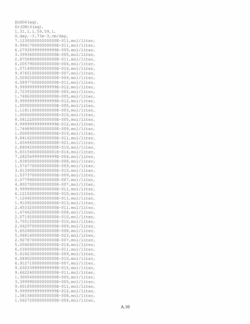
A.10
ZnSO4(aq), Zr(OH)4(aq), 1,31,1,1,59,59,1, 0,day,-3.73e-3,cm/day, 7.123050000000000E-011,mol/liter, 9.994170000000000E-011,mol/liter, 6.279359999999999E-005,mol/liter, 3.399360000000000E-005,mol/liter, 2.875080000000000E-011,mol/liter, 6.205790000000000E-006,mol/liter, 1.071490000000000E-016,mol/liter, 9.476510000000000E-007,mol/liter, 3.509220000000000E-004,mol/liter, 4.589770000000000E-011,mol/liter, 9.999999999999999E-012,mol/liter, 2.723930000000000E-005,mol/liter, 1.748630000000000E-005,mol/liter, 9.999999999999999E-012,mol/liter, 1.000000000000000E-005,mol/liter, 1.118110000000000E-003,mol/liter, 1.000000000000000E-010,mol/liter, 8.581220000000000E-005,mol/liter, 9.999999999999999E-012,mol/liter, 1.744890000000000E-009,mol/liter, 1.000000000000000E-010,mol/liter, 9.841620000000000E-011,mol/liter, 1.654940000000000E-021,mol/liter, 2.880420000000000E-010,mol/liter, 5.831540000000001E-014,mol/liter, 7.282569999999999E-004,mol/liter, 1.838500000000000E-008,mol/liter, 1.574770000000000E-009,mol/liter, 3.613900000000000E-010,mol/liter, 1.537370000000000E-009,mol/liter, 2.077990000000000E-007,mol/liter, 4.802700000000000E-007,mol/liter, 9.999990000000000E-011,mol/liter, 6.121020000000000E-010,mol/liter, 7.124920000000000E-011,mol/liter, 1.910920000000000E-013,mol/liter, 2.453320000000000E-011,mol/liter, 1.474620000000000E-008,mol/liter, 2.071920000000000E-010,mol/liter, 3.755150000000000E-010,mol/liter, 2.062970000000000E-009,mol/liter, 5.652680000000000E-008,mol/liter, 5.968140000000000E-023,mol/liter, 2.927870000000000E-007,mol/liter, 5.006060000000000E-014,mol/liter, 6.534500000000000E-011,mol/liter, 5.618230000000000E-009,mol/liter, 6.089020000000000E-010,mol/liter, 6.912710000000000E-007,mol/liter, 9.630339999999999E-015,mol/liter, 9.662240000000000E-011,mol/liter, 1.300540000000000E-005,mol/liter, 3.399990000000000E-005,mol/liter, 9.601850000000000E-011,mol/liter, 9.999999999999999E-012,mol/liter, 1.581580000000000E-008,mol/liter, 1.562720000000000E-004,mol/liter,
A.11
Bottom,Unit Gradient,Aqueous Species Outflow, 0, 1,31,1,1,1,1,1, 0,yr,,,,,,,, ~Inactive Nodes Card 0, ~Source Card 0, ~Output Control Card 31, 1,1,1, 2,1,1, 3,1,1, 4,1,1, 5,1,1, 6,1,1, 7,1,1, 8,1,1, 9,1,1, 10,1,1, 11,1,1, 12,1,1, 13,1,1, 14,1,1, 15,1,1, 16,1,1, 17,1,1, 18,1,1, 19,1,1, 20,1,1, 21,1,1, 22,1,1, 23,1,1, 24,1,1, 25,1,1, 26,1,1, 27,1,1, 28,1,1, 29,1,1, 30,1,1, 31,1,1, 1,1,day,cm,deg,6,6,6, 3, Species Aqueous Concentration,Total_B(OH)3(aq),mol/liter, Species Aqueous Concentration,Total_MoO4--,mol/liter, Species Aqueous Concentration,H+,mol/liter, 15, 0,sec, 1,sec, 1313,day, 1325,day, 1346,day, 1411,day, 1676,day, 1683,day, 1690,day, 1698,day, 1712,day,
A.12
1726,day, 1738,day, 1747,day, 10,yr, 113, Diffusive Porosity,, Aqueous Relative Permeability,, Aqueous Pressure,Pa, Aqueous Density,kg/m^3, Aqueous Moisture Content,, Aqueous Saturation,, Temperature,, xnc Aqueous Volumetric Flux,m/s, znc Aqueous Volumetric Flux,m/s, Species Aqueous Concentration,Al+++,mol/liter, Species Aqueous Concentration,B(OH)3(aq),mol/liter, Species Aqueous Concentration,Ca++,mol/liter, Species Aqueous Concentration,Cl-,mol/liter, Species Aqueous Concentration,CrO4--,mol/liter, Species Aqueous Concentration,F-,mol/liter, Species Aqueous Concentration,Fe+++,mol/liter, Species Aqueous Concentration,H+,mol/liter, Species Aqueous Concentration,HCO3-,mol/liter, Species Aqueous Concentration,HPO4--,mol/liter, Species Aqueous Concentration,I-,mol/liter, Species Aqueous Concentration,K+,mol/liter, Species Aqueous Concentration,Mg++,mol/liter, Species Aqueous Concentration,MoO4--,mol/liter, Species Aqueous Concentration,NO3-,mol/liter, Species Aqueous Concentration,Na+,mol/liter, Species Aqueous Concentration,ReO4-,mol/liter, Species Aqueous Concentration,SO4--,mol/liter, Species Aqueous Concentration,SeO3--,mol/liter, Species Aqueous Concentration,SiO2(aq),mol/liter, Species Aqueous Concentration,Ti(OH)4(aq),mol/liter, Species Aqueous Concentration,Zn++,mol/liter, Species Aqueous Concentration,Zr(OH)2++,mol/liter, Species Aqueous Concentration,AlO2-,mol/liter, Species Aqueous Concentration,BO2-,mol/liter, Species Aqueous Concentration,CO2(aq),mol/liter, Species Aqueous Concentration,CO3--,mol/liter, Species Aqueous Concentration,CaCO3(aq),mol/liter, Species Aqueous Concentration,CaCl+,mol/liter, Species Aqueous Concentration,CaF+,mol/liter, Species Aqueous Concentration,CaHCO3+,mol/liter, Species Aqueous Concentration,CaSO4(aq),mol/liter, Species Aqueous Concentration,Fe(OH)3(aq),mol/liter, Species Aqueous Concentration,H2PO4-,mol/liter, Species Aqueous Concentration,HCrO4-,mol/liter, Species Aqueous Concentration,HSiO3-,mol/liter, Species Aqueous Concentration,KCl(aq),mol/liter, Species Aqueous Concentration,KSO4-,mol/liter, Species Aqueous Concentration,MgCO3(aq),mol/liter, Species Aqueous Concentration,MgCl+,mol/liter, Species Aqueous Concentration,MgF+,mol/liter, Species Aqueous Concentration,MgHCO3+,mol/liter, Species Aqueous Concentration,MgP2O7--,mol/liter, Species Aqueous Concentration,MgSO4(aq),mol/liter, Species Aqueous Concentration,NaAlO2(aq),mol/liter, Species Aqueous Concentration,NaCO3-,mol/liter, Species Aqueous Concentration,NaCl(aq),mol/liter,
A.13
Species Aqueous Concentration,NaF(aq),mol/liter, Species Aqueous Concentration,NaHCO3(aq),mol/liter, Species Aqueous Concentration,NaHSiO3(aq),mol/liter, Species Aqueous Concentration,NaOH(aq),mol/liter, Species Aqueous Concentration,OH-,mol/liter, Species Aqueous Concentration,PO4---,mol/liter, Species Aqueous Concentration,ZnCl+,mol/liter, Species Aqueous Concentration,ZnCl2(aq),mol/liter, Species Aqueous Concentration,ZnSO4(aq),mol/liter, Species Aqueous Concentration,Zr(OH)4(aq),mol/liter, Species Volume Fraction,Albite_high,, Species Volume Fraction,Analcime,, Species Volume Fraction,Anatase,, Species Volume Fraction,Baddeleyite,, Species Volume Fraction,Calcite,, Species Volume Fraction,Chalcedony,, Species Volume Fraction,Clinochlore-14A,, Species Volume Fraction,Fe(OH)3,, Species Volume Fraction,Gibbsite,, Species Volume Fraction,K-Feldspar,, Species Volume Fraction,LAWA44,, Species Volume Fraction,LAWA44-H,, Species Volume Fraction,Muscovite,, Species Volume Fraction,Quartz,, Species Volume Fraction,Sepiolite,, Species Volume Fraction,Tremolite,, Species Volume Fraction,Zn(OH)2(gamma),, Species Aqueous Concentration,CaX2,mol/liter, Species Aqueous Concentration,KX,mol/liter, Species Aqueous Concentration,MgX2,mol/liter, Species Aqueous Concentration,NaX,mol/liter, Species Aqueous Concentration,Total_AlO2-,mol/liter, Species Aqueous Concentration,Total_B(OH)3(aq),mol/liter, Species Aqueous Concentration,Total_Ca++,mol/liter, Species Aqueous Concentration,Total_Cl-,mol/liter, Species Aqueous Concentration,Total_CrO4--,mol/liter, Species Aqueous Concentration,Total_F-,mol/liter, Species Aqueous Concentration,Total_Fe(OH)3(aq),mol/liter, Species Aqueous Concentration,Total_HCO3-,mol/liter, Species Aqueous Concentration,Total_HPO4--,mol/liter, Species Aqueous Concentration,Total_I-,mol/liter, Species Aqueous Concentration,Total_K+,mol/liter, Species Aqueous Concentration,Total_Mg++,mol/liter, Species Aqueous Concentration,Total_MoO4--,mol/liter, Species Aqueous Concentration,Total_NO3-,mol/liter, Species Aqueous Concentration,Total_Na+,mol/liter, Species Aqueous Concentration,Total_SO4--,mol/liter, Species Aqueous Concentration,Total_SiO2(aq),mol/liter, Species Aqueous Concentration,Total_SeO3--,mol/liter, Species Aqueous Concentration,Total_ReO4-,mol/liter, Species Aqueous Concentration,Total_Ti(OH)4(aq),mol/liter, Species Aqueous Concentration,Total_Zn++,mol/liter, Species Aqueous Concentration,Total_Zr(OH)4(aq),mol/L, Exchange Species Aqueous Concentration,total_NaX,mol/L, Exchange Species Volumetric Concentration,total_NaX,mol/L, Aqueous Courant,, Final Restart,, ~Surface Flux Card 3, Conservation Component Mass Flux,Total_B(OH)3(aq),mol/yr,mol,Bottom,1,31,1,1,1,1,

A.14
Conservation Component Mass Flux,Total_MoO4--,mol/yr,mol,Bottom,1,31,1,1,1,1, Aqueous Volumetric Flux,cm^3/day,cm^3,Bottom,1,31,1,1,1,1,
B.1
Appendix B: Hydraulic Property Analysis of Lysimeter Backfill Hydraulic property analyses of Phil Meyer’s samples Mart Oostrom, 1/27/05 Sample Names D10-D11-D14-Fill-Top-1 D10-D11-D14-Fill-Top-2 D10-D11 D14-Fill-1 D14-Fill-2 Particle Density Three replicates of the particle density test were performed using the pycnometer method (Blake and Hartge 1986) Sample Particle Density (g/cm3) D10-D11-D14-Fill-Top-1 2.72 D10-D11-D14-Fill-Top-2 2.73 D10-D11 2.71 D14-Fill-1 2.67 D14-Fill-2 2.68 Hydraulic Conductivity (Method: Constant head hydraulic conductivity; Klute and Dirksen, 1986) Reported values are averages of 3 measurements each for 3 different imposed heads. Sample Ksat (x 10-4) cm/s Standard Deviation (x 10-4)
cm/s D10-D11-D14-Fill-Top-1 7.33 1.03 D10-D11-D14-Fill-Top-2 9.12 1.08 D10-D11 9.04 0.77 D14-Fill-1 6.07 1.34 D14-Fill-2 5.04 0.73 Particle Size Distribution The PSD test was performed using the methods ASTM Standard C.29 and Gee and Bauder (1986). An analysis has been completed for samples D10-D11-D14-Fill-1, D10-11, and D14-Fill-1. The full analysis data of these samples are reported in accompanied Excel files. Sample File Name USDA Soil Type D10-D11-D14-Fill-Top-1 PSA-D10-D11-D14-Fill-Top-
1.xls Loamy sand
D10-D11 PSA-D10-D11.xls Sandy Loam D14-Fill-1 PSA-D14-Fill-1.xls Sandy Loam
B.2
Water Retention Water retention data for the samples were obtained using the EMSL saturation-pressure apparatus for pressure head up to 500 cm. The pressure plate method (Klute, 1986) was used to obtain water contents at 0.5, 1, 2, and 4 bar. The complete experimental data sets, analysis results, and plots are located in the Excel files listed below. In the subsequent table, an overview of the main fitting results is presented. Sample File D10-D11-D14-Fill-Top-1 vgfit_d10-d11-d14_fill_top_1.xls D10-D11-D14-Fill-Top-2 vgfit-d10-d11-d14-fill-top-2.xls D10-D11 vgfit_d10-d11.xls D14-Fill-1 vgfit_d14_fill_1.xls D14-Fill-2 vgfit_d14_fill_2.xls Sample VG alpha
(1/cm) VG n Theta s Theta r
D10-D11-D14-Fill-Top-1 0.006 2.20 0.385 0.012 D10-D11-D14-Fill-Top-2 0.006 2.32 0.387 0.015 D10-D11 0.009 2.23 0.405 0.017 D14-Fill-1 0.005 2.77 0.394 0.042 D14-Fill-2 0.004 2.66 0.407 0.036 Steady-State Constant Flux Test Steady-state constant flux tests were performed for three samples (2 relative permeabilities for each sample). The results are listed in the tables below. The experiments were done with 10-cm-long columns with a 5 cm inside diameter. The columns were equipped with 2 tensiometers, located 2.5 cm from either end. A flux was applied consistent with a relative permeability of either 0.2 or 0.1, based on the saturated hydraulic conductivity. The bottom outlet was lowered 1 cm at the time. It was assumed that unit gradient conditions were obtained when the pressures at both tensiometer locations were within 1 cm. Sample: D10-D11-D14-Fill-Top-1 Relative perm Saturation Suction (cm) upper
transducer Suction (cm) lower transducer
0.2 0.81 72.1 72.9 0.1 0.63 104.3 103.7 Sample: D10-D11 Relative perm Saturation Suction (cm) upper
transducer Suction (cm) lower transducer
0.2 0.74 80.4 81.3 0.1 0.53 111.7 112.5 Sample: D14-Fill-1 Relative perm Saturation Suction (cm) upper
transducer Suction (cm) lower transducer
0.2 0.70 60.4 60.8 0.1 0.58 99.2 99.8
C.1
Appendix C: Geochemist’s Workbench Input File for LAWA44 in Columbia River water
# React script, saved Thu Dec 10 2015 by D3A926
data = "..\thermo.com.V8.r6+_lysimeter.dat" verify
temperature = 15
H2O = 1 free kg
swap O2(g) for O2(aq)
O2(g) = -.7 log fugacity
swap CO2(g) for HCO3-
CO2(g) = -3.5 log fugacity
Ca++ = .0004407 molal
Mg++ = .00017796 molal
Na+ = 5.1296e-5 molal
K+ = 1.9098e-5 molal
Cl- = 3.3985e-5 molal
F- = 6.219e-6 molal
HPO4-- = 6.5862e-10 molal
swap NO3- for NH3(aq)
NO3- = 1.001e-5 molal
SO4-- = 8.6604e-5 molal
H+ = 1.6604e-8 molal
swap AlO2- for Al+++
AlO2- = 1e-10 molal
B(OH)3(aq) = 1e-10 molal
CrO4-- = 1e-10 molal
swap Fe(OH)3(aq) for Fe++
Fe(OH)3(aq) = 1e-10 molal
SiO2(aq) = 1e-10 molal
Ti(OH)4(aq) = 1e-10 molal
Zn++ = 1e-10 molal
swap Zr(OH)4(aq) for Zr(OH)2++
Zr(OH)4(aq) = 1e-10 molal
C.2
ReO4- = 1e-10 molal
MoO4-- = 1e-10 molal
SeO3-- = 1e-10 molal
I- = 1e-10 molal
balance off
reactants times 100
react .00041 mol of Al2O3
react .000863 mol of B2O3
react 6.19e-5 mol of HCl
react 8.88e-7 mol of Cr2O3
react 1.78e-6 mol of HF
react .000295 mol of Fe2O3
react 3.58e-5 mol of K2O
react .000333 mol of MgO
react .00218 mol of Na2O
react 1.43e-6 mol of P2O5
react 8.43e-6 mol of SO3
react .00498 mol of SiO2
react .000168 mol of TiO2
react .000246 mol of ZnO
react .000164 mol of Baddeleyite
fix fugacity of O2(g)
fix fugacity of CO2(g)
react .00024 mol of CaO
react 3.09e-6 mol of Re
react 4.69e-6 mol of Mo
react 5.32E-06 mol of HI
react 6.08e-6 mol of SeO2
suppress ALL
unsuppress Analcime Anatase Baddeleyite Chalcedony
unsuppress Fe(OH)3 Gibbsite Zn(OH)2(gamma)
alter Analcime 10.14 9.14 7.584 6.011 4.408 3.108 1.985 .927
alter Fe(OH)3 10.5 9.156 7.604 6.188 4.777 3.615 2.587 1.616
alter Sepiolite 47.39 45.44 42.17 38.9 35.72 33.33 31.41 29.67
alter Anatase 500 -6.559 -6.559 -6.559 500 500 500 500
alter Baddeleyite -5.604 -5.441 -5.278 -5.172 -5.132 -5.152 -5.216 -5.314
alter Chalcedony -4.036 -3.428 -2.931 -2.562 -2.228 -1.967 -1.751 -1.576
alter Zn(OH)2(gamma) 500 11.88 11.88 11.88 500 500 500 500
delxi = .01 log
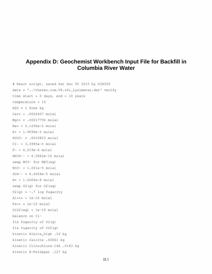
D.1
Appendix D: Geochemist Workbench Input File for Backfill in Columbia River Water
# React script, saved Sat Dec 05 2015 by D3A926
data = "..\thermo.com.V8.r6+_lysimeter.dat" verify
time start = 0 days, end = 10 years
temperature = 15
H2O = 1 free kg
Ca++ = .0004407 molal
Mg++ = .00017796 molal
Na+ = 5.1296e-5 molal
K+ = 1.9098e-5 molal
HCO3- = .0010823 molal
Cl- = 3.3985e-5 molal
F- = 6.219e-6 molal
HPO4-- = 6.5862e-10 molal
swap NO3- for NH3(aq)
NO3- = 1.001e-5 molal
SO4-- = 8.6604e-5 molal
H+ = 1.6604e-8 molal
swap O2(g) for O2(aq)
O2(g) = -.7 log fugacity
Al+++ = 1e-10 molal
Fe++ = 1e-10 molal
SiO2(aq) = 1e-10 molal
balance on Cl-
fix fugacity of O2(g)
fix fugacity of CO2(g)
kinetic Albite_high .16 kg
kinetic Calcite .00061 kg
kinetic Clinochlore-14A .0183 kg
kinetic K-Feldspar .127 kg
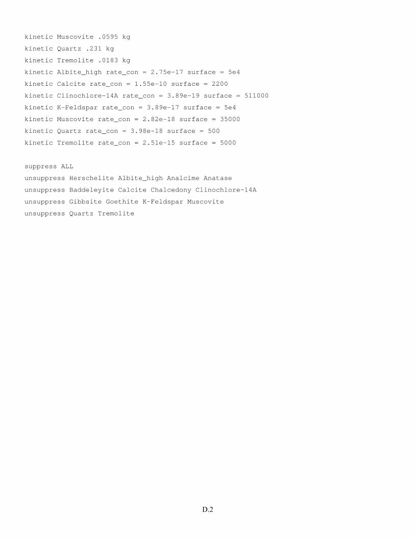
D.2
kinetic Muscovite .0595 kg
kinetic Quartz .231 kg
kinetic Tremolite .0183 kg
kinetic Albite_high rate_con = 2.75e-17 surface = 5e4
kinetic Calcite rate_con = 1.55e-10 surface = 2200
kinetic Clinochlore-14A rate_con = 3.89e-19 surface = 511000
kinetic K-Feldspar rate_con = 3.89e-17 surface = 5e4
kinetic Muscovite rate_con = 2.82e-18 surface = 35000
kinetic Quartz rate_con = 3.98e-18 surface = 500
kinetic Tremolite rate_con = 2.51e-15 surface = 5000
suppress ALL
unsuppress Herschelite Albite_high Analcime Anatase
unsuppress Baddeleyite Calcite Chalcedony Clinochlore-14A
unsuppress Gibbsite Goethite K-Feldspar Muscovite
unsuppress Quartz Tremolite
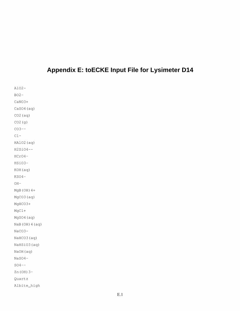
E.1
Appendix E: toECKE Input File for Lysimeter D14
AlO2-
BO2-
CaNO3+
CaSO4(aq)
CO2(aq)
CO2(g)
CO3--
Cl-
HAlO2(aq)
H2SiO4--
HCrO4-
HSiO3-
KOH(aq)
KSO4-
OH-
MgB(OH)4+
MgCO3(aq)
MgHCO3+
MgCl+
MgSO4(aq)
NaB(OH)4(aq)
NaCO3-
NaHCO3(aq)
NaHSiO3(aq)
NaOH(aq)
NaSO4-
SO4--
Zn(OH)3-
Quartz
Albite_high
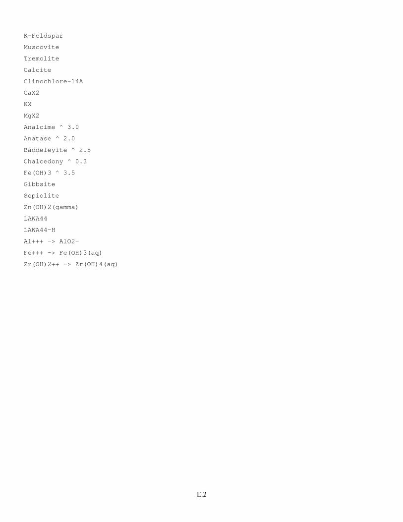
E.2
K-Feldspar
Muscovite
Tremolite
Calcite
Clinochlore-14A
CaX2
KX
MgX2
Analcime ^ 3.0
Anatase ^ 2.0
Baddeleyite ^ 2.5
Chalcedony ^ 0.3
Fe(OH)3 ^ 3.5
Gibbsite
Sepiolite
Zn(OH)2(gamma)
LAWA44
LAWA44-H
Al+++ -> AlO2-
Fe+++ -> Fe(OH)3(aq)
Zr(OH)2++ -> Zr(OH)4(aq)
F.1
Appendix F: Input File for Perko et al. (2015) Case 0
~Simulation Title Card
1,
Decalcification of cracked cement structures by Perko et al.,
Yilin Fang,
PNNL,
June 2015,
,
1,
case 0, conservative tracer,
#
~Solution Control Card
normal,
Water w/transport ,
1,
0.0,d,100,d,0.01,d,1,d,1.25,8,1.e-06,
10000,
0,
# Follow GEMs grid in Perko et al.
~Grid Card
cartesian,
101,1,105,
#
0,mm,0.25,mm,0.5,mm,0.625,mm,[email protected],mm,25,mm,
0,mm,1.0,mm,
0,mm,[email protected],mm,[email protected],mm,[email protected],mm,[email protected],mm,[email protected],mm,
#
~Rock/Soil Zonation Card
3,
F.2
cement, 1,101,1,1,1,105,
crack,1,2,1,1,51, 100,
top,1,101,1,1,101,105,
#
~Mechanical Properties Card
top,,, 0.3,0.3,,,constant,0.0383,
cement,,,0.1,0.1,,,constant,0.0383,
crack,,,1,1,,,constant,1,
#
~Hydraulic Properties Card
top,1E-9,hc:m/s, 1E-9,hc:m/s,1E-9,hc:m/s,
cement, 5E-10,hc:m/s,5E-10,hc:m/s,5E-10,hc:m/s,
crack,4.1E-1,hc:m/s, 4.1E-1,hc:m/s,4.1E-1,hc:m/s,
#
~Saturation Function Card
top,van Genuchten, 1.43,1/m,1.506,,,
crack,van Genuchten, 1.43,1/m,1.506,,,
cement,van Genuchten, 1.43,1/m,1.506,,,
#
~Aqueous Relative Permeability Card
top, Mualem,,
cement,Mualem,,
crack,Mualem,,
#
~Solute/Fluid Interaction Card
1,
tracer,constant,1e-9,m^2/s,continuous,1e20,yr,
0,
#
~Solute/Porous Media Interaction Card
top,0.1,m,0.1,m,
tracer,0.0,,
cement,0.1,m,0.1,m,
tracer,0.0,,
F.3
crack,0.1,m,0.1,m,
tracer,0.0,,
#
~Initial Conditions Card
Gas Pressure,Aqueous Pressure,
3,
Gas Pressure, 101325,Pa,,,,,,, 1,101,1,1,1,105,
Aqueous Pressure,110628,pa,,,,,-9793,1/m,1,101,1,1,1,105,
Solute aqueous volumetric,tracer,1e-3,1/L,,,,,,1/m,1,101,1,1,1,100,
#
~Boundary Conditions Card
2,
top,neumann,aqueous conc,
1,101,1,1,105,105,1,
0.0,d,0.0,mm/yr,0.0,1/L,
bottom,dirichlet,,
1,101,1,1,1,1,1,
0.0,d,110628,pa,,,
#
~Output Control Card
206,
#x = 5mm
21,1,1,
21,1,2,
21,1,3,
21,1,4,
21,1,5,
21,1,6,
21,1,7,
21,1,8,
21,1,9,
21,1,10,
21,1,11,
21,1,12,
21,1,13,
21,1,14,
F.4
21,1,15,
21,1,16,
21,1,17,
21,1,18,
21,1,19,
21,1,20,
21,1,21,
21,1,22,
21,1,23,
21,1,24,
21,1,25,
21,1,26,
21,1,27,
21,1,28,
21,1,29,
21,1,30,
21,1,31,
21,1,32,
21,1,33,
21,1,34,
21,1,35,
21,1,36,
21,1,37,
21,1,38,
21,1,39,
21,1,40,
21,1,41,
21,1,42,
21,1,43,
21,1,44,
21,1,45,
21,1,46,
21,1,47,
21,1,48,
21,1,49,
21,1,50,
21,1,51,
21,1,52,
21,1,53,
21,1,54,
F.5
21,1,55,
21,1,56,
21,1,57,
21,1,58,
21,1,59,
21,1,60,
21,1,61,
21,1,62,
21,1,63,
21,1,64,
21,1,65,
21,1,66,
21,1,67,
21,1,68,
21,1,69,
21,1,70,
21,1,71,
21,1,72,
21,1,73,
21,1,74,
21,1,75,
21,1,76,
21,1,77,
21,1,78,
21,1,79,
21,1,80,
21,1,81,
21,1,82,
21,1,83,
21,1,84,
21,1,85,
21,1,86,
21,1,87,
21,1,88,
21,1,89,
21,1,90,
21,1,91,
21,1,92,
21,1,93,
21,1,94,
F.6
21,1,95,
21,1,96,
21,1,97,
21,1,98,
21,1,99,
21,1,100,
21,1,101,
21,1,102,
21,1,103,
21,1,104,
21,1,105,
#y=90mm
1,1,90,
2,1,90,
3,1,90,
4,1,90,
5,1,90,
6,1,90,
7,1,90,
8,1,90,
9,1,90,
10,1,90,
11,1,90,
12,1,90,
13,1,90,
14,1,90,
15,1,90,
16,1,90,
17,1,90,
18,1,90,
19,1,90,
20,1,90,
21,1,90,
22,1,90,
23,1,90,
24,1,90,
25,1,90,
26,1,90,
27,1,90,
28,1,90,
F.7
29,1,90,
30,1,90,
31,1,90,
32,1,90,
33,1,90,
34,1,90,
35,1,90,
36,1,90,
37,1,90,
38,1,90,
39,1,90,
40,1,90,
41,1,90,
42,1,90,
43,1,90,
44,1,90,
45,1,90,
46,1,90,
47,1,90,
48,1,90,
49,1,90,
50,1,90,
51,1,90,
52,1,90,
53,1,90,
54,1,90,
55,1,90,
56,1,90,
57,1,90,
58,1,90,
59,1,90,
60,1,90,
61,1,90,
62,1,90,
63,1,90,
64,1,90,
65,1,90,
66,1,90,
67,1,90,
68,1,90,
F.8
69,1,90,
70,1,90,
71,1,90,
72,1,90,
73,1,90,
74,1,90,
75,1,90,
76,1,90,
77,1,90,
78,1,90,
79,1,90,
80,1,90,
81,1,90,
82,1,90,
83,1,90,
84,1,90,
85,1,90,
86,1,90,
87,1,90,
88,1,90,
89,1,90,
90,1,90,
91,1,90,
92,1,90,
93,1,90,
94,1,90,
95,1,90,
96,1,90,
97,1,90,
98,1,90,
99,1,90,
100,1,90,
101,1,90,
1,1,d,m,6,6,6,
1,
solute aqueous conc,tracer,1/L,
1,
0,day,
1,
solute aqueous conc,tracer,1/L,
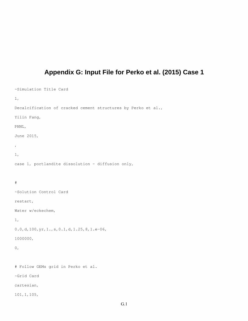
G.1
Appendix G: Input File for Perko et al. (2015) Case 1
~Simulation Title Card
1,
Decalcification of cracked cement structures by Perko et al.,
Yilin Fang,
PNNL,
June 2015,
,
1,
case 1, portlandite dissolution - diffusion only,
#
~Solution Control Card
restart,
Water w/eckechem,
1,
0.0,d,100,yr,1.,s,0.1,d,1.25,8,1.e-06,
1000000,
0,
# Follow GEMs grid in Perko et al.
~Grid Card
cartesian,
101,1,105,
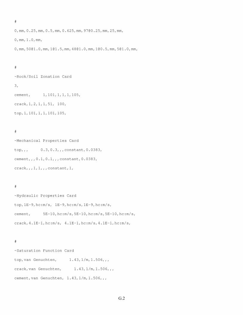
G.2
#
0,mm,0.25,mm,0.5,mm,0.625,mm,[email protected],mm,25,mm,
0,mm,1.0,mm,
0,mm,[email protected],mm,[email protected],mm,[email protected],mm,[email protected],mm,[email protected],mm,
#
~Rock/Soil Zonation Card
3,
cement, 1,101,1,1,1,105,
crack,1,2,1,1,51, 100,
top,1,101,1,1,101,105,
#
~Mechanical Properties Card
top,,, 0.3,0.3,,,constant,0.0383,
cement,,,0.1,0.1,,,constant,0.0383,
crack,,,1,1,,,constant,1,
#
~Hydraulic Properties Card
top,1E-9,hc:m/s, 1E-9,hc:m/s,1E-9,hc:m/s,
cement, 5E-10,hc:m/s,5E-10,hc:m/s,5E-10,hc:m/s,
crack,4.1E-1,hc:m/s, 4.1E-1,hc:m/s,4.1E-1,hc:m/s,
#
~Saturation Function Card
top,van Genuchten, 1.43,1/m,1.506,,,
crack,van Genuchten, 1.43,1/m,1.506,,,
cement,van Genuchten, 1.43,1/m,1.506,,,
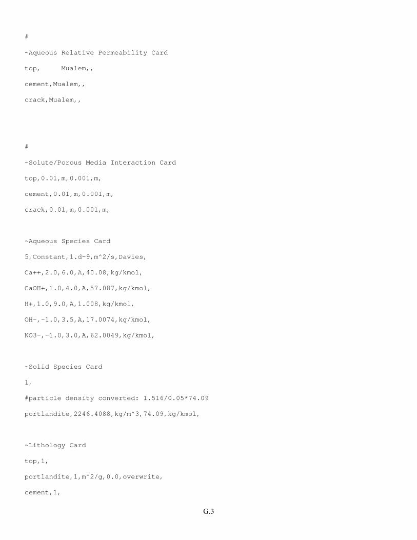
G.3
#
~Aqueous Relative Permeability Card
top, Mualem,,
cement,Mualem,,
crack,Mualem,,
#
~Solute/Porous Media Interaction Card
top,0.01,m,0.001,m,
cement,0.01,m,0.001,m,
crack,0.01,m,0.001,m,
~Aqueous Species Card
5,Constant,1.d-9,m^2/s,Davies,
Ca++,2.0,6.0,A,40.08,kg/kmol,
CaOH+,1.0,4.0,A,57.087,kg/kmol,
H+,1.0,9.0,A,1.008,kg/kmol,
OH-,-1.0,3.5,A,17.0074,kg/kmol,
NO3-,-1.0,3.0,A,62.0049,kg/kmol,
~Solid Species Card
1,
#particle density converted: 1.516/0.05*74.09
portlandite,2246.4088,kg/m^3,74.09,kg/kmol,
~Lithology Card
top,1,
portlandite,1,m^2/g,0.0,overwrite,
cement,1,
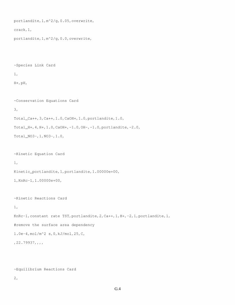
G.4
portlandite,1,m^2/g,0.05,overwrite,
crack,1,
portlandite,1,m^2/g,0.0,overwrite,
~Species Link Card
1,
H+,pH,
~Conservation Equations Card
3,
Total_Ca++,3,Ca++,1.0,CaOH+,1.0,portlandite,1.0,
Total_H+,4,H+,1.0,CaOH+,-1.0,OH-,-1.0,portlandite,-2.0,
Total_NO3-,1,NO3-,1.0,
~Kinetic Equation Card
1,
Kinetic_portlandite,1,portlandite,1.00000e+00,
1,KnRc-1,1.00000e+00,
~Kinetic Reactions Card
1,
KnRc-1,constant rate TST,portlandite,2,Ca++,1,H+,-2,1,portlandite,1,
#remove the surface area dependency
1.0e-4,mol/m^2 s,0,kJ/mol,25,C,
,22.79937,,,,
~Equilibrium Reactions Card
2,
G.5
EqRc-1,0.0,-13.998,0.0,0.0,0.0,1/mol,
EqRc-2,0.0,-12.780,0.0,0.0,0.0,1/mol,
~Equilibrium Equations Card
2,
2,OH-,H+,-1.00000e+00,EqRc-1,1.0,
3,CaOH+,Ca++,1.00000e+00,H+,-1.00000e+00,EqRc-2,1.0,
#
~Initial Conditions Card
Gas Pressure,Aqueous Pressure,
3,
#Gas Pressure, 101325,Pa,,,,,,, 1,101,1,1,1,105,
#Aqueous Pressure,110628,pa,,,,,-9793,1/m,1,101,1,1,1,105,
overwrite Species Aqueous Volumetric,pH,12.48,,,,,,,,1,101,1,1,1,100,
#overwrite Species Aqueous Volumetric,H+,1.948d-07,mol/liter,,,,,,,1,101,1,1,101,105,
overwrite Species Aqueous Volumetric,pH,6.71,,,,,,,,1,101,1,1,101,105,
overwrite Species Aqueous Volumetric,Ca++,1.948d-02,mol/liter,,,,,,,1,101,1,1,1,100,
#
~Boundary Conditions Card
2,
top,neumann,species aqueous conc,
3,H+,no3-,ca++,
1,101,1,1,105,105,1,
0.0,d,0.0,mm/yr,
1e-3,mol/L,1.035e-3,mol/L,1.e-16,mol/l,
bottom,dirichlet,,
0,
G.6
1,101,1,1,1,1,1,
0.0,d,110628,pa,
#
~Output Control Card
206,
#x = 5mm,105 cell vertical
21,1,1,
21,1,2,
21,1,3,
21,1,4,
21,1,5,
21,1,6,
21,1,7,
21,1,8,
21,1,9,
21,1,10,
21,1,11,
21,1,12,
21,1,13,
21,1,14,
21,1,15,
21,1,16,
21,1,17,
21,1,18,
21,1,19,
21,1,20,
21,1,21,
21,1,22,
G.7
21,1,23,
21,1,24,
21,1,25,
21,1,26,
21,1,27,
21,1,28,
21,1,29,
21,1,30,
21,1,31,
21,1,32,
21,1,33,
21,1,34,
21,1,35,
21,1,36,
21,1,37,
21,1,38,
21,1,39,
21,1,40,
21,1,41,
21,1,42,
21,1,43,
21,1,44,
21,1,45,
21,1,46,
21,1,47,
21,1,48,
21,1,49,
21,1,50,
21,1,51,
21,1,52,
G.8
21,1,53,
21,1,54,
21,1,55,
21,1,56,
21,1,57,
21,1,58,
21,1,59,
21,1,60,
21,1,61,
21,1,62,
21,1,63,
21,1,64,
21,1,65,
21,1,66,
21,1,67,
21,1,68,
21,1,69,
21,1,70,
21,1,71,
21,1,72,
21,1,73,
21,1,74,
21,1,75,
21,1,76,
21,1,77,
21,1,78,
21,1,79,
21,1,80,
21,1,81,
21,1,82,
G.9
21,1,83,
21,1,84,
21,1,85,
21,1,86,
21,1,87,
21,1,88,
21,1,89,
21,1,90,
21,1,91,
21,1,92,
21,1,93,
21,1,94,
21,1,95,
21,1,96,
21,1,97,
21,1,98,
21,1,99,
21,1,100,
21,1,101,
21,1,102,
21,1,103,
21,1,104,
21,1,105,
#y=75mm
1,1,75,
2,1,75,
3,1,75,
4,1,75,
5,1,75,
6,1,75,
G.10
7,1,75,
8,1,75,
9,1,75,
10,1,75,
11,1,75,
12,1,75,
13,1,75,
14,1,75,
15,1,75,
16,1,75,
17,1,75,
18,1,75,
19,1,75,
20,1,75,
21,1,75,
22,1,75,
23,1,75,
24,1,75,
25,1,75,
26,1,75,
27,1,75,
28,1,75,
29,1,75,
30,1,75,
31,1,75,
32,1,75,
33,1,75,
34,1,75,
35,1,75,
36,1,75,

G.11
37,1,75,
38,1,75,
39,1,75,
40,1,75,
41,1,75,
42,1,75,
43,1,75,
44,1,75,
45,1,75,
46,1,75,
47,1,75,
48,1,75,
49,1,75,
50,1,75,
51,1,75,
52,1,75,
53,1,75,
54,1,75,
55,1,75,
56,1,75,
57,1,75,
58,1,75,
59,1,75,
60,1,75,
61,1,75,
62,1,75,
63,1,75,
64,1,75,
65,1,75,
66,1,75,
G.12
67,1,75,
68,1,75,
69,1,75,
70,1,75,
71,1,75,
72,1,75,
73,1,75,
74,1,75,
75,1,75,
76,1,75,
77,1,75,
78,1,75,
79,1,75,
80,1,75,
81,1,75,
82,1,75,
83,1,75,
84,1,75,
85,1,75,
86,1,75,
87,1,75,
88,1,75,
89,1,75,
90,1,75,
91,1,75,
92,1,75,
93,1,75,
94,1,75,
95,1,75,
96,1,75,
G.13
97,1,75,
98,1,75,
99,1,75,
100,1,75,
101,1,75,
1,1,yr,m,6,6,6,
3,
species volumetric conc,portlandite,mol/L,
species aqueous conc,total_Ca++,mol/L,
#species aqueous conc,H+,mol/L,
pH,,
1,
9,yr,
3,
species volumetric conc,portlandite,mol/L,
species aqueous conc,ca++,mol/L,
species aqueous conc,h+,mol/L,
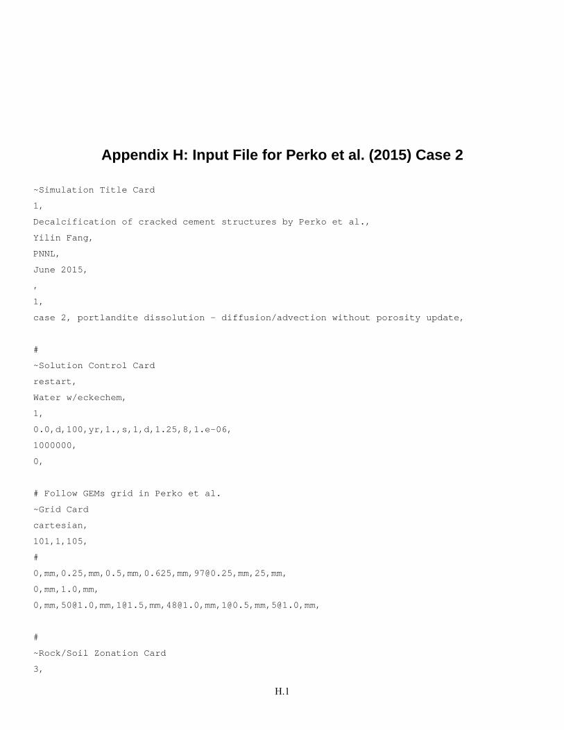
H.1
Appendix H: Input File for Perko et al. (2015) Case 2
~Simulation Title Card
1,
Decalcification of cracked cement structures by Perko et al.,
Yilin Fang,
PNNL,
June 2015,
,
1,
case 2, portlandite dissolution - diffusion/advection without porosity update,
#
~Solution Control Card
restart,
Water w/eckechem,
1,
0.0,d,100,yr,1.,s,1,d,1.25,8,1.e-06,
1000000,
0,
# Follow GEMs grid in Perko et al.
~Grid Card
cartesian,
101,1,105,
#
0,mm,0.25,mm,0.5,mm,0.625,mm,[email protected],mm,25,mm,
0,mm,1.0,mm,
0,mm,[email protected],mm,[email protected],mm,[email protected],mm,[email protected],mm,[email protected],mm,
#
~Rock/Soil Zonation Card
3,
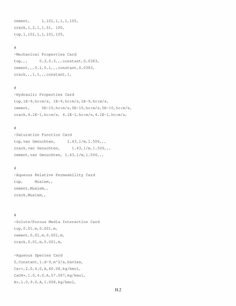
H.2
cement, 1,101,1,1,1,105,
crack,1,2,1,1,51, 100,
top,1,101,1,1,101,105,
#
~Mechanical Properties Card
top,,, 0.3,0.3,,,constant,0.0383,
cement,,,0.1,0.1,,,constant,0.0383,
crack,,,1,1,,,constant,1,
#
~Hydraulic Properties Card
top,1E-9,hc:m/s, 1E-9,hc:m/s,1E-9,hc:m/s,
cement, 5E-10,hc:m/s,5E-10,hc:m/s,5E-10,hc:m/s,
crack,4.1E-1,hc:m/s, 4.1E-1,hc:m/s,4.1E-1,hc:m/s,
#
~Saturation Function Card
top,van Genuchten, 1.43,1/m,1.506,,,
crack,van Genuchten, 1.43,1/m,1.506,,,
cement,van Genuchten, 1.43,1/m,1.506,,,
#
~Aqueous Relative Permeability Card
top, Mualem,,
cement,Mualem,,
crack,Mualem,,
#
~Solute/Porous Media Interaction Card
top,0.01,m,0.001,m,
cement,0.01,m,0.001,m,
crack,0.01,m,0.001,m,
~Aqueous Species Card
5,Constant,1.d-9,m^2/s,Davies,
Ca++,2.0,6.0,A,40.08,kg/kmol,
CaOH+,1.0,4.0,A,57.087,kg/kmol,
H+,1.0,9.0,A,1.008,kg/kmol,
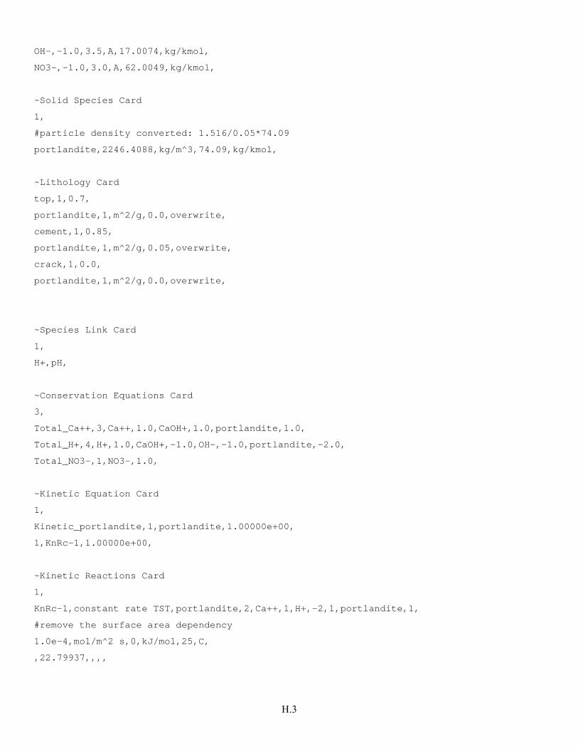
H.3
OH-,-1.0,3.5,A,17.0074,kg/kmol,
NO3-,-1.0,3.0,A,62.0049,kg/kmol,
~Solid Species Card
1,
#particle density converted: 1.516/0.05*74.09
portlandite,2246.4088,kg/m^3,74.09,kg/kmol,
~Lithology Card
top,1,0.7,
portlandite,1,m^2/g,0.0,overwrite,
cement,1,0.85,
portlandite,1,m^2/g,0.05,overwrite,
crack,1,0.0,
portlandite,1,m^2/g,0.0,overwrite,
~Species Link Card
1,
H+,pH,
~Conservation Equations Card
3,
Total_Ca++,3,Ca++,1.0,CaOH+,1.0,portlandite,1.0,
Total_H+,4,H+,1.0,CaOH+,-1.0,OH-,-1.0,portlandite,-2.0,
Total_NO3-,1,NO3-,1.0,
~Kinetic Equation Card
1,
Kinetic_portlandite,1,portlandite,1.00000e+00,
1,KnRc-1,1.00000e+00,
~Kinetic Reactions Card
1,
KnRc-1,constant rate TST,portlandite,2,Ca++,1,H+,-2,1,portlandite,1,
#remove the surface area dependency
1.0e-4,mol/m^2 s,0,kJ/mol,25,C,
,22.79937,,,,
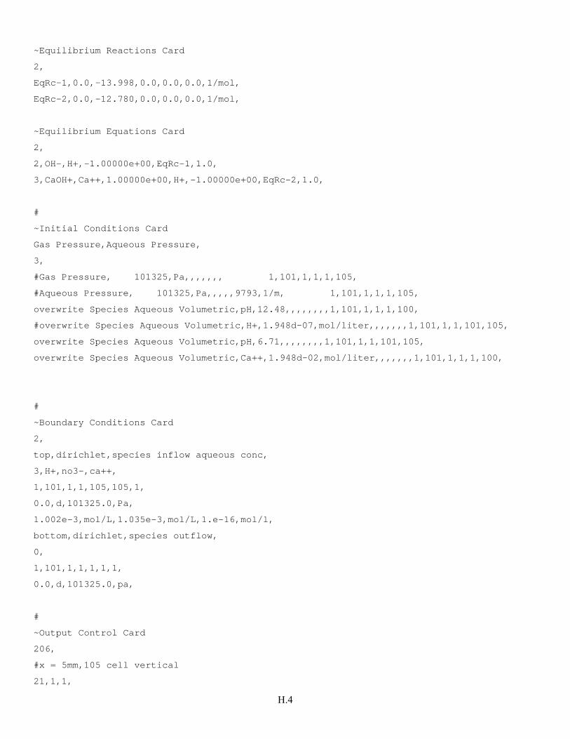
H.4
~Equilibrium Reactions Card
2,
EqRc-1,0.0,-13.998,0.0,0.0,0.0,1/mol,
EqRc-2,0.0,-12.780,0.0,0.0,0.0,1/mol,
~Equilibrium Equations Card
2,
2,OH-,H+,-1.00000e+00,EqRc-1,1.0,
3,CaOH+,Ca++,1.00000e+00,H+,-1.00000e+00,EqRc-2,1.0,
#
~Initial Conditions Card
Gas Pressure,Aqueous Pressure,
3,
#Gas Pressure, 101325,Pa,,,,,,, 1,101,1,1,1,105,
#Aqueous Pressure, 101325,Pa,,,,,9793,1/m, 1,101,1,1,1,105,
overwrite Species Aqueous Volumetric,pH,12.48,,,,,,,,1,101,1,1,1,100,
#overwrite Species Aqueous Volumetric,H+,1.948d-07,mol/liter,,,,,,,1,101,1,1,101,105,
overwrite Species Aqueous Volumetric,pH,6.71,,,,,,,,1,101,1,1,101,105,
overwrite Species Aqueous Volumetric,Ca++,1.948d-02,mol/liter,,,,,,,1,101,1,1,1,100,
#
~Boundary Conditions Card
2,
top,dirichlet,species inflow aqueous conc,
3,H+,no3-,ca++,
1,101,1,1,105,105,1,
0.0,d,101325.0,Pa,
1.002e-3,mol/L,1.035e-3,mol/L,1.e-16,mol/l,
bottom,dirichlet,species outflow,
0,
1,101,1,1,1,1,1,
0.0,d,101325.0,pa,
#
~Output Control Card
206,
#x = 5mm,105 cell vertical
21,1,1,
H.5
21,1,2,
21,1,3,
21,1,4,
21,1,5,
21,1,6,
21,1,7,
21,1,8,
21,1,9,
21,1,10,
21,1,11,
21,1,12,
21,1,13,
21,1,14,
21,1,15,
21,1,16,
21,1,17,
21,1,18,
21,1,19,
21,1,20,
21,1,21,
21,1,22,
21,1,23,
21,1,24,
21,1,25,
21,1,26,
21,1,27,
21,1,28,
21,1,29,
21,1,30,
21,1,31,
21,1,32,
21,1,33,
21,1,34,
21,1,35,
21,1,36,
21,1,37,
21,1,38,
21,1,39,
21,1,40,
21,1,41,
H.6
21,1,42,
21,1,43,
21,1,44,
21,1,45,
21,1,46,
21,1,47,
21,1,48,
21,1,49,
21,1,50,
21,1,51,
21,1,52,
21,1,53,
21,1,54,
21,1,55,
21,1,56,
21,1,57,
21,1,58,
21,1,59,
21,1,60,
21,1,61,
21,1,62,
21,1,63,
21,1,64,
21,1,65,
21,1,66,
21,1,67,
21,1,68,
21,1,69,
21,1,70,
21,1,71,
21,1,72,
21,1,73,
21,1,74,
21,1,75,
21,1,76,
21,1,77,
21,1,78,
21,1,79,
21,1,80,
21,1,81,
H.7
21,1,82,
21,1,83,
21,1,84,
21,1,85,
21,1,86,
21,1,87,
21,1,88,
21,1,89,
21,1,90,
21,1,91,
21,1,92,
21,1,93,
21,1,94,
21,1,95,
21,1,96,
21,1,97,
21,1,98,
21,1,99,
21,1,100,
21,1,101,
21,1,102,
21,1,103,
21,1,104,
21,1,105,
#y=75mm
1,1,75,
2,1,75,
3,1,75,
4,1,75,
5,1,75,
6,1,75,
7,1,75,
8,1,75,
9,1,75,
10,1,75,
11,1,75,
12,1,75,
13,1,75,
14,1,75,
15,1,75,
H.8
16,1,75,
17,1,75,
18,1,75,
19,1,75,
20,1,75,
21,1,75,
22,1,75,
23,1,75,
24,1,75,
25,1,75,
26,1,75,
27,1,75,
28,1,75,
29,1,75,
30,1,75,
31,1,75,
32,1,75,
33,1,75,
34,1,75,
35,1,75,
36,1,75,
37,1,75,
38,1,75,
39,1,75,
40,1,75,
41,1,75,
42,1,75,
43,1,75,
44,1,75,
45,1,75,
46,1,75,
47,1,75,
48,1,75,
49,1,75,
50,1,75,
51,1,75,
52,1,75,
53,1,75,
54,1,75,
55,1,75,
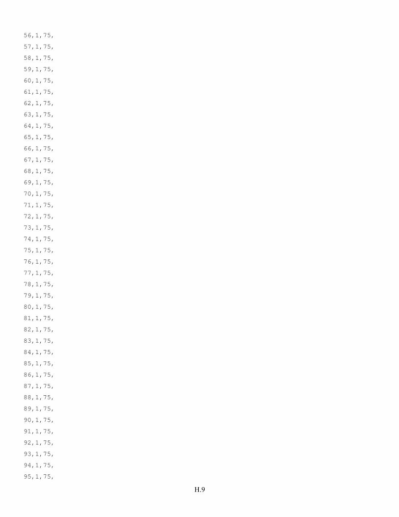
H.9
56,1,75,
57,1,75,
58,1,75,
59,1,75,
60,1,75,
61,1,75,
62,1,75,
63,1,75,
64,1,75,
65,1,75,
66,1,75,
67,1,75,
68,1,75,
69,1,75,
70,1,75,
71,1,75,
72,1,75,
73,1,75,
74,1,75,
75,1,75,
76,1,75,
77,1,75,
78,1,75,
79,1,75,
80,1,75,
81,1,75,
82,1,75,
83,1,75,
84,1,75,
85,1,75,
86,1,75,
87,1,75,
88,1,75,
89,1,75,
90,1,75,
91,1,75,
92,1,75,
93,1,75,
94,1,75,
95,1,75,
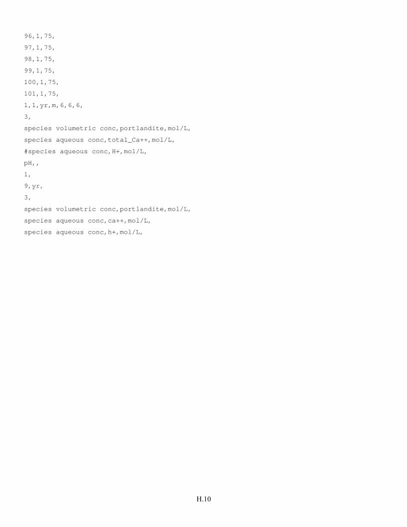
H.10
96,1,75,
97,1,75,
98,1,75,
99,1,75,
100,1,75,
101,1,75,
1,1,yr,m,6,6,6,
3,
species volumetric conc,portlandite,mol/L,
species aqueous conc,total_Ca++,mol/L,
#species aqueous conc,H+,mol/L,
pH,,
1,
9,yr,
3,
species volumetric conc,portlandite,mol/L,
species aqueous conc,ca++,mol/L,
species aqueous conc,h+,mol/L,
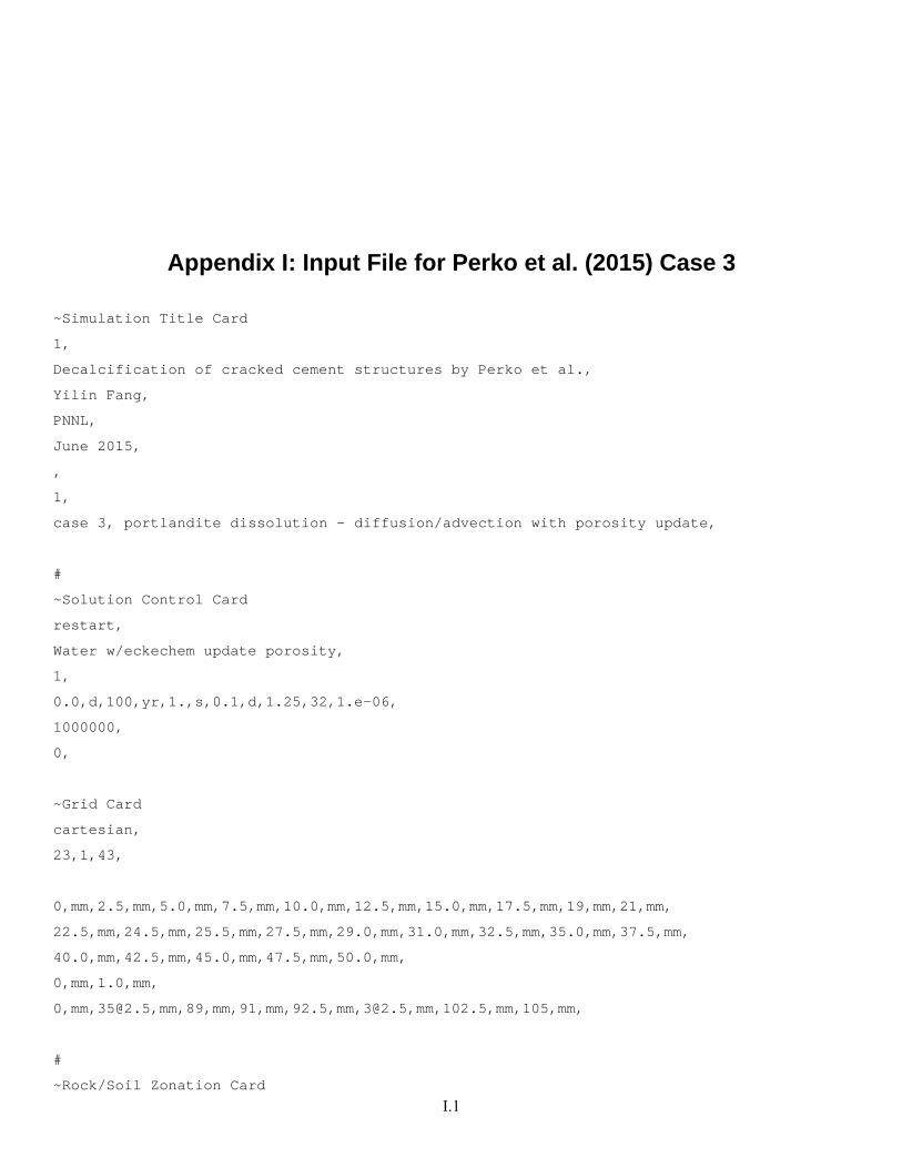
I.1
Appendix I: Input File for Perko et al. (2015) Case 3
~Simulation Title Card
1,
Decalcification of cracked cement structures by Perko et al.,
Yilin Fang,
PNNL,
June 2015,
,
1,
case 3, portlandite dissolution - diffusion/advection with porosity update,
#
~Solution Control Card
restart,
Water w/eckechem update porosity,
1,
0.0,d,100,yr,1.,s,0.1,d,1.25,32,1.e-06,
1000000,
0,
~Grid Card
cartesian,
23,1,43,
0,mm,2.5,mm,5.0,mm,7.5,mm,10.0,mm,12.5,mm,15.0,mm,17.5,mm,19,mm,21,mm,
22.5,mm,24.5,mm,25.5,mm,27.5,mm,29.0,mm,31.0,mm,32.5,mm,35.0,mm,37.5,mm,
40.0,mm,42.5,mm,45.0,mm,47.5,mm,50.0,mm,
0,mm,1.0,mm,
0,mm,[email protected],mm,89,mm,91,mm,92.5,mm,[email protected],mm,102.5,mm,105,mm,
#
~Rock/Soil Zonation Card
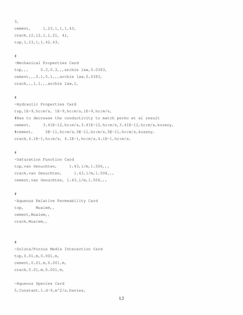
I.2
3,
cement, 1,23,1,1,1,43,
crack,12,12,1,1,21, 41,
top,1,23,1,1,42,43,
#
~Mechanical Properties Card
top,,, 0.3,0.3,,,archie law,0.0383,
cement,,,0.1,0.1,,,archie law,0.0383,
crack,,,1,1,,,archie law,1,
#
~Hydraulic Properties Card
top,1E-9,hc:m/s, 1E-9,hc:m/s,1E-9,hc:m/s,
#Has to decrease the conductivity to match perko et al result
cement, 3.41E-12,hc:m/s,3.41E-12,hc:m/s,3.41E-12,hc:m/s,kozeny,
#cement, 5E-11,hc:m/s,5E-11,hc:m/s,5E-11,hc:m/s,kozeny,
crack,4.1E-1,hc:m/s, 4.1E-1,hc:m/s,4.1E-1,hc:m/s,
#
~Saturation Function Card
top,van Genuchten, 1.43,1/m,1.506,,,
crack,van Genuchten, 1.43,1/m,1.506,,,
cement,van Genuchten, 1.43,1/m,1.506,,,
#
~Aqueous Relative Permeability Card
top, Mualem,,
cement,Mualem,,
crack,Mualem,,
#
~Solute/Porous Media Interaction Card
top,0.01,m,0.001,m,
cement,0.01,m,0.001,m,
crack,0.01,m,0.001,m,
~Aqueous Species Card
5,Constant,1.d-9,m^2/s,Davies,
I.3
Ca++, 2.0, 6.0,A, 40.0780,kg/kmol,
CaOH+, 1.0, 4.0,A, 57.0853,kg/kmol,
H+, 1.0, 9.0,A, 1.0079,kg/kmol,
NO3-, -1.0, 3.0,A, 62.0049,kg/kmol,
OH-, -1.0, 3.5,A, 17.0073,kg/kmol,
~Solid Species Card
1,
#particle density converted: 1.516/0.05*74.09
portlandite,2246.4088,kg/m^3,74.09,kg/kmol,
~Lithology Card
top,1,0.7,
portlandite,1,m^2/g,0.0,overwrite,
cement,1,0.85,
portlandite,1,m^2/g,0.05,overwrite,
crack,1,0.0,
portlandite,1,m^2/g,0.0,overwrite,
~Species Link Card
1,
H+,pH,
~Conservation Equations Card
3,
Total_Ca++, 3,Ca++, 1.0000E+00,CaOH+, 1.0000E+00,Portlandite, 1.0000E+00,
Total_H+, 4,CaOH+,-1.0000E+00,H+, 1.0000E+00,OH-,-1.0000E+00,Portlandite,-2.0000E+00,
Total_NO3-, 1,NO3-, 1.0000E+00,
~Kinetic Equation Card
1,
Kinetic_Portlandite,1,Portlandite,1,
1,KnRc-3, 1.0000,
~Kinetic Reactions Card
1,
KnRc-3,constant rate TST,Portlandite, 1,Ca++, 1.0000E+00, 2,H+, 2.0000E+00,Portlandite, 1.0000E+00,
#remove the surface area dependency
I.4
1.0e-4,mol/m^2 s,0,kJ/mol,25,C,
,22.79937,,,,
~Equilibrium Reactions Card
2,
EqRc-1, 0.0000000E+00,-1.2780000E+01, 0.0000000E+00, 0.0000000E+00, 0.0000000E+00,
EqRc-2, 0.0000000E+00,-1.3998000E+01, 0.0000000E+00, 0.0000000E+00, 0.0000000E+00,
~Equilibrium Equations Card
2,
3,CaOH+,Ca++, 1.0000,H+, -1.0000,EqRc-1, 1.0000,
2,OH-,H+, -1.0000,EqRc-2, 1.0000,
#
~Initial Conditions Card
Gas Pressure,Aqueous Pressure,
3,
#Gas Pressure, 101325,Pa,,,,,,, 1,23,1,1,1,43,
#Aqueous Pressure, 101325,Pa,,,,,,, 1,23,1,1,1,43,
overwrite Species Aqueous Volumetric,pH,12.48,,,,,,,,1,23,1,1,1,41,
#overwrite Species Aqueous Volumetric,H+,1.948d-07,mol/liter,,,,,,,1,23,1,1,42,43,
overwrite Species Aqueous Volumetric,pH,6.71,,,,,,,,1,23,1,1,42,43,
overwrite Species Aqueous Volumetric,Ca++,1.948d-02,mol/liter,,,,,,,1,23,1,1,1,41,
#
~Boundary Conditions Card
2,
top,dirichlet,species aqueous conc,
3,H+,no3-,ca++,
1,23,1,1,43,43,1,
0.0,d,101325.0,Pa,
1e-3,mol/L,1.035e-3,mol/L,0.e-16,mol/l,
#bottom,dirichlet,zero flux,
bottom,dirichlet,species outflow,
0,
1,23,1,1,1,1,1,
0.0,d,101325.0,pa,
I.5
#
~Output Control Card
55,
15,1,1,
15,1,2,
15,1,3,
15,1,4,
15,1,5,
15,1,6,
15,1,7,
15,1,8,
15,1,9,
15,1,10,
15,1,11,
15,1,12,
15,1,13,
15,1,14,
15,1,15,
15,1,16,
15,1,17,
15,1,18,
15,1,19,
15,1,20,
15,1,21,
15,1,22,
15,1,23,
15,1,24,
15,1,25,
15,1,26,
15,1,27,
15,1,28,
15,1,29,
15,1,30,
15,1,31,
15,1,32,
15,1,33,
15,1,34,
15,1,35,
15,1,36,
15,1,37,
I.6
15,1,38,
15,1,39,
15,1,40,
15,1,41,
15,1,42,
15,1,43,
12,1,30,
13,1,30,
14,1,30,
15,1,30,
16,1,30,
17,1,30,
18,1,30,
19,1,30,
20,1,30,
21,1,30,
22,1,30,
23,1,30,
1,1,yr,m,6,6,6,
5,
species volumetric conc,portlandite,mol/L,
species aqueous conc,total_Ca++,mol/L,
#species aqueous conc,H+,mol/L,
pH,,
diffusive porosity,,
znc aqueous saturation,,
1,
9,yr,
3,
species volumetric conc,portlandite,mol/L,
species aqueous conc,ca++,mol/L,
species aqueous conc,h+,mol/L,
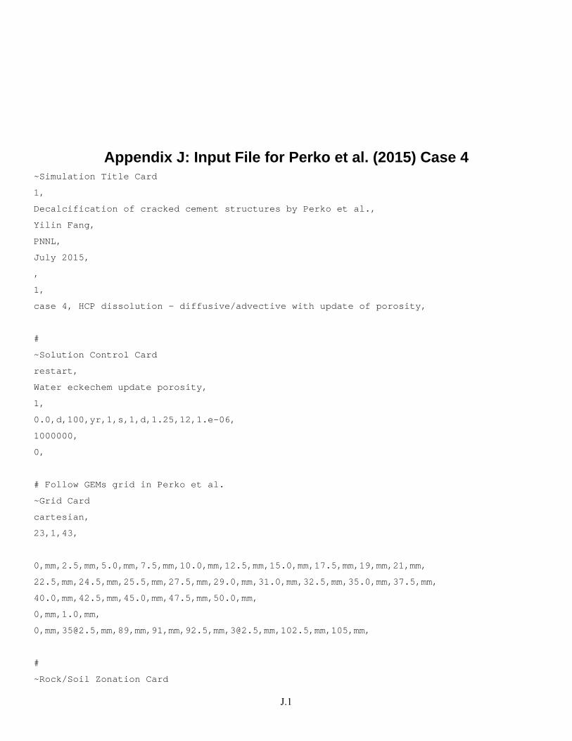
J.1
Appendix J: Input File for Perko et al. (2015) Case 4 ~Simulation Title Card
1,
Decalcification of cracked cement structures by Perko et al.,
Yilin Fang,
PNNL,
July 2015,
,
1,
case 4, HCP dissolution - diffusive/advective with update of porosity,
#
~Solution Control Card
restart,
Water eckechem update porosity,
1,
0.0,d,100,yr,1,s,1,d,1.25,12,1.e-06,
1000000,
0,
# Follow GEMs grid in Perko et al.
~Grid Card
cartesian,
23,1,43,
0,mm,2.5,mm,5.0,mm,7.5,mm,10.0,mm,12.5,mm,15.0,mm,17.5,mm,19,mm,21,mm,
22.5,mm,24.5,mm,25.5,mm,27.5,mm,29.0,mm,31.0,mm,32.5,mm,35.0,mm,37.5,mm,
40.0,mm,42.5,mm,45.0,mm,47.5,mm,50.0,mm,
0,mm,1.0,mm,
0,mm,[email protected],mm,89,mm,91,mm,92.5,mm,[email protected],mm,102.5,mm,105,mm,
#
~Rock/Soil Zonation Card
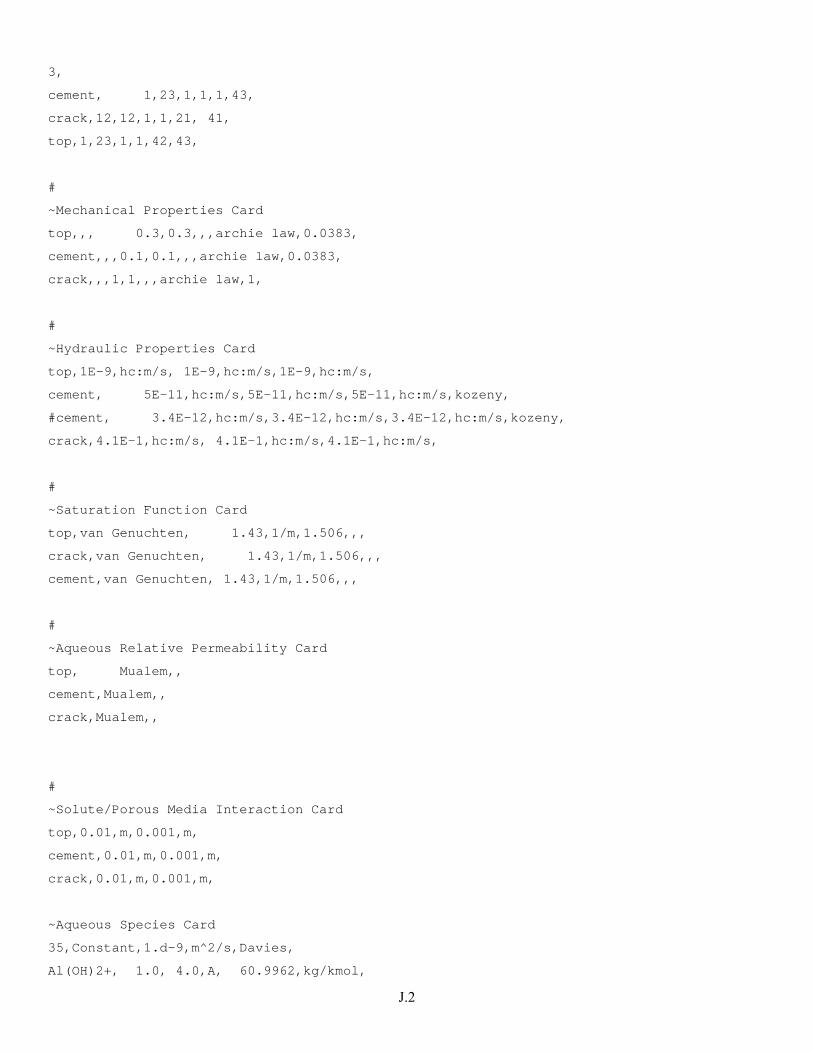
J.2
3,
cement, 1,23,1,1,1,43,
crack,12,12,1,1,21, 41,
top,1,23,1,1,42,43,
#
~Mechanical Properties Card
top,,, 0.3,0.3,,,archie law,0.0383,
cement,,,0.1,0.1,,,archie law,0.0383,
crack,,,1,1,,,archie law,1,
#
~Hydraulic Properties Card
top,1E-9,hc:m/s, 1E-9,hc:m/s,1E-9,hc:m/s,
cement, 5E-11,hc:m/s,5E-11,hc:m/s,5E-11,hc:m/s,kozeny,
#cement, 3.4E-12,hc:m/s,3.4E-12,hc:m/s,3.4E-12,hc:m/s,kozeny,
crack,4.1E-1,hc:m/s, 4.1E-1,hc:m/s,4.1E-1,hc:m/s,
#
~Saturation Function Card
top,van Genuchten, 1.43,1/m,1.506,,,
crack,van Genuchten, 1.43,1/m,1.506,,,
cement,van Genuchten, 1.43,1/m,1.506,,,
#
~Aqueous Relative Permeability Card
top, Mualem,,
cement,Mualem,,
crack,Mualem,,
#
~Solute/Porous Media Interaction Card
top,0.01,m,0.001,m,
cement,0.01,m,0.001,m,
crack,0.01,m,0.001,m,
~Aqueous Species Card
35,Constant,1.d-9,m^2/s,Davies,
Al(OH)2+, 1.0, 4.0,A, 60.9962,kg/kmol,
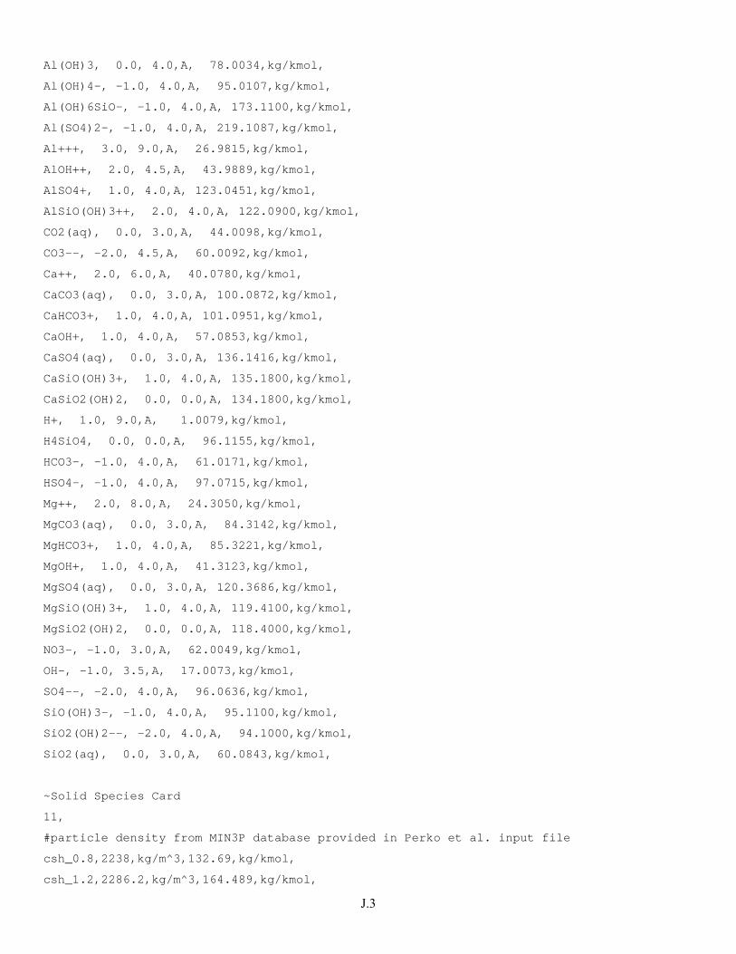
J.3
Al(OH)3, 0.0, 4.0,A, 78.0034,kg/kmol,
Al(OH)4-, -1.0, 4.0,A, 95.0107,kg/kmol,
Al(OH)6SiO-, -1.0, 4.0,A, 173.1100,kg/kmol,
Al(SO4)2-, -1.0, 4.0,A, 219.1087,kg/kmol,
Al+++, 3.0, 9.0,A, 26.9815,kg/kmol,
AlOH++, 2.0, 4.5,A, 43.9889,kg/kmol,
AlSO4+, 1.0, 4.0,A, 123.0451,kg/kmol,
AlSiO(OH)3++, 2.0, 4.0,A, 122.0900,kg/kmol,
CO2(aq), 0.0, 3.0,A, 44.0098,kg/kmol,
CO3--, -2.0, 4.5,A, 60.0092,kg/kmol,
Ca++, 2.0, 6.0,A, 40.0780,kg/kmol,
CaCO3(aq), 0.0, 3.0,A, 100.0872,kg/kmol,
CaHCO3+, 1.0, 4.0,A, 101.0951,kg/kmol,
CaOH+, 1.0, 4.0,A, 57.0853,kg/kmol,
CaSO4(aq), 0.0, 3.0,A, 136.1416,kg/kmol,
CaSiO(OH)3+, 1.0, 4.0,A, 135.1800,kg/kmol,
CaSiO2(OH)2, 0.0, 0.0,A, 134.1800,kg/kmol,
H+, 1.0, 9.0,A, 1.0079,kg/kmol,
H4SiO4, 0.0, 0.0,A, 96.1155,kg/kmol,
HCO3-, -1.0, 4.0,A, 61.0171,kg/kmol,
HSO4-, -1.0, 4.0,A, 97.0715,kg/kmol,
Mg++, 2.0, 8.0,A, 24.3050,kg/kmol,
MgCO3(aq), 0.0, 3.0,A, 84.3142,kg/kmol,
MgHCO3+, 1.0, 4.0,A, 85.3221,kg/kmol,
MgOH+, 1.0, 4.0,A, 41.3123,kg/kmol,
MgSO4(aq), 0.0, 3.0,A, 120.3686,kg/kmol,
MgSiO(OH)3+, 1.0, 4.0,A, 119.4100,kg/kmol,
MgSiO2(OH)2, 0.0, 0.0,A, 118.4000,kg/kmol,
NO3-, -1.0, 3.0,A, 62.0049,kg/kmol,
OH-, -1.0, 3.5,A, 17.0073,kg/kmol,
SO4--, -2.0, 4.0,A, 96.0636,kg/kmol,
SiO(OH)3-, -1.0, 4.0,A, 95.1100,kg/kmol,
SiO2(OH)2--, -2.0, 4.0,A, 94.1000,kg/kmol,
SiO2(aq), 0.0, 3.0,A, 60.0843,kg/kmol,
~Solid Species Card
11,
#particle density from MIN3P database provided in Perko et al. input file
csh_0.8,2238,kg/m^3,132.69,kg/kmol,
csh_1.2,2286.2,kg/m^3,164.489,kg/kmol,
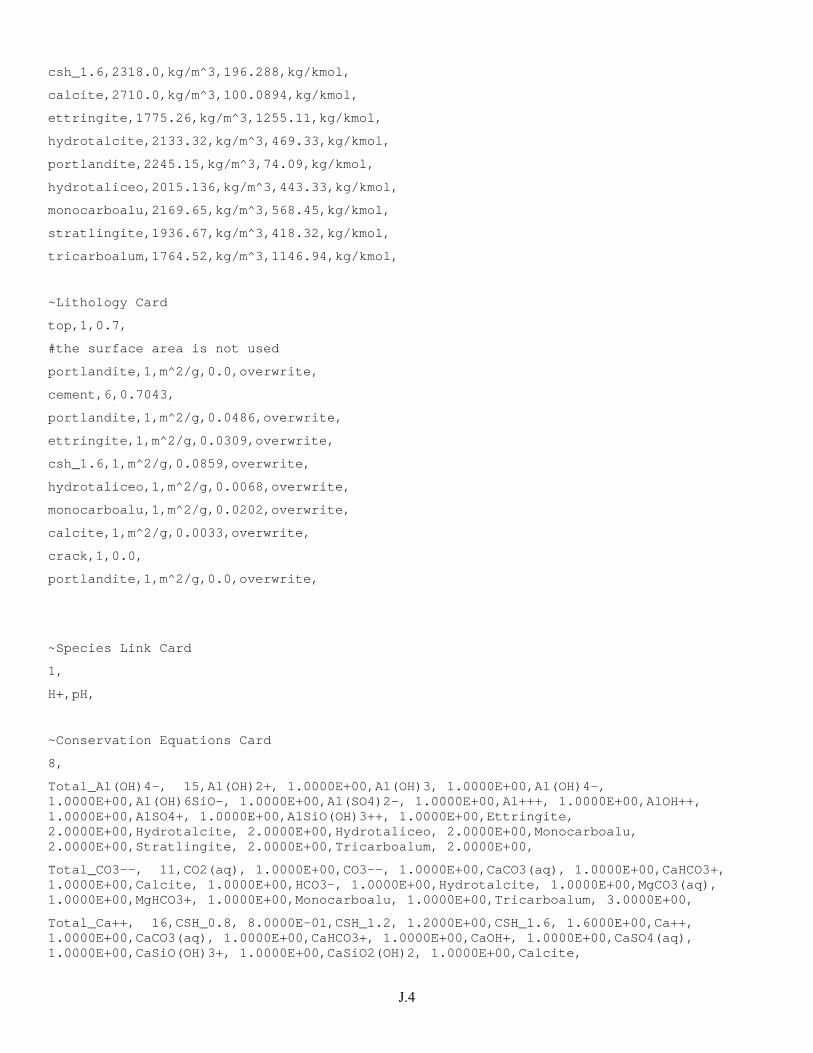
J.4
csh_1.6,2318.0,kg/m^3,196.288,kg/kmol,
calcite,2710.0,kg/m^3,100.0894,kg/kmol,
ettringite,1775.26,kg/m^3,1255.11,kg/kmol,
hydrotalcite,2133.32,kg/m^3,469.33,kg/kmol,
portlandite,2245.15,kg/m^3,74.09,kg/kmol,
hydrotaliceo,2015.136,kg/m^3,443.33,kg/kmol,
monocarboalu,2169.65,kg/m^3,568.45,kg/kmol,
stratlingite,1936.67,kg/m^3,418.32,kg/kmol,
tricarboalum,1764.52,kg/m^3,1146.94,kg/kmol,
~Lithology Card
top,1,0.7,
#the surface area is not used
portlandite,1,m^2/g,0.0,overwrite,
cement,6,0.7043,
portlandite,1,m^2/g,0.0486,overwrite,
ettringite,1,m^2/g,0.0309,overwrite,
csh_1.6,1,m^2/g,0.0859,overwrite,
hydrotaliceo,1,m^2/g,0.0068,overwrite,
monocarboalu,1,m^2/g,0.0202,overwrite,
calcite,1,m^2/g,0.0033,overwrite,
crack,1,0.0,
portlandite,1,m^2/g,0.0,overwrite,
~Species Link Card
1,
H+,pH,
~Conservation Equations Card
8,
Total_Al(OH)4-, 15,Al(OH)2+, 1.0000E+00,Al(OH)3, 1.0000E+00,Al(OH)4-, 1.0000E+00,Al(OH)6SiO-, 1.0000E+00,Al(SO4)2-, 1.0000E+00,Al+++, 1.0000E+00,AlOH++, 1.0000E+00,AlSO4+, 1.0000E+00,AlSiO(OH)3++, 1.0000E+00,Ettringite, 2.0000E+00,Hydrotalcite, 2.0000E+00,Hydrotaliceo, 2.0000E+00,Monocarboalu, 2.0000E+00,Stratlingite, 2.0000E+00,Tricarboalum, 2.0000E+00,
Total_CO3--, 11,CO2(aq), 1.0000E+00,CO3--, 1.0000E+00,CaCO3(aq), 1.0000E+00,CaHCO3+, 1.0000E+00,Calcite, 1.0000E+00,HCO3-, 1.0000E+00,Hydrotalcite, 1.0000E+00,MgCO3(aq), 1.0000E+00,MgHCO3+, 1.0000E+00,Monocarboalu, 1.0000E+00,Tricarboalum, 3.0000E+00,
Total_Ca++, 16,CSH_0.8, 8.0000E-01,CSH_1.2, 1.2000E+00,CSH_1.6, 1.6000E+00,Ca++, 1.0000E+00,CaCO3(aq), 1.0000E+00,CaHCO3+, 1.0000E+00,CaOH+, 1.0000E+00,CaSO4(aq), 1.0000E+00,CaSiO(OH)3+, 1.0000E+00,CaSiO2(OH)2, 1.0000E+00,Calcite,
J.5
1.0000E+00,Ettringite, 6.0000E+00,Monocarboalu, 4.0000E+00,Portlandite, 1.0000E+00,Stratlingite, 2.0000E+00,Tricarboalum, 6.0000E+00,
Total_H+, 32,Al(OH)2+, 2.0000E+00,Al(OH)3, 1.0000E+00,Al(SO4)2-, 4.0000E+00,Al+++, 4.0000E+00,AlOH++, 3.0000E+00,AlSO4+, 4.0000E+00,AlSiO(OH)3++, 3.0000E+00,CO2(aq), 2.0000E+00,CSH_0.8,-1.6000E+00,CSH_1.2,-2.4000E+00,CSH_1.6,-3.2000E+00,
CaHCO3+, 1.0000E+00,CaOH+,-1.0000E+00,CaSiO(OH)3+,-1.0000E+00,CaSiO2(OH)2,-2.0000E+00,Ettringite,-4.0000E+00,H+, 1.0000E+00,HCO3-, 1.0000E+00,HSO4-, 1.0000E+00,Hydrotalcite,-4.0000E+00,Hydrotaliceo,-6.0000E+00,MgHCO3+, 1.0000E+00,MgOH+,-1.0000E+00,MgSiO(OH)3+,-1.0000E+00,
MgSiO2(OH)2,-2.0000E+00,Monocarboalu,-4.0000E+00,OH-,-1.0000E+00,Portlandite,-2.0000E+00,SiO(OH)3-,-1.0000E+00,SiO2(OH)2--,-2.0000E+00,Stratlingite,-2.0000E+00,Tricarboalum,-4.0000E+00,
Total_H4SiO4, 14,Al(OH)6SiO-, 1.0000E+00,AlSiO(OH)3++, 1.0000E+00,CSH_0.8, 1.0000E+00,CSH_1.2, 1.0000E+00,CSH_1.6, 1.0000E+00,CaSiO(OH)3+, 1.0000E+00,CaSiO2(OH)2, 1.0000E+00,H4SiO4, 1.0000E+00,MgSiO(OH)3+, 1.0000E+00,MgSiO2(OH)2, 1.0000E+00,SiO(OH)3-, 1.0000E+00,SiO2(OH)2--, 1.0000E+00,SiO2(aq), 1.0000E+00,Stratlingite, 1.0000E+00,
Total_Mg++, 9,Hydrotalcite, 4.0000E+00,Hydrotaliceo, 4.0000E+00,Mg++, 1.0000E+00,MgCO3(aq), 1.0000E+00,MgHCO3+, 1.0000E+00,MgOH+, 1.0000E+00,MgSO4(aq), 1.0000E+00,MgSiO(OH)3+, 1.0000E+00,MgSiO2(OH)2, 1.0000E+00,
Total_NO3-, 1,NO3-, 1.0000E+00,
Total_SO4--, 7,Al(SO4)2-, 2.0000E+00,AlSO4+, 1.0000E+00,CaSO4(aq), 1.0000E+00,Ettringite, 3.0000E+00,HSO4-, 1.0000E+00,MgSO4(aq), 1.0000E+00,SO4--, 1.0000E+00,
~Kinetic Equation Card
11,
Kinetic_CSH_0.8,1,CSH_0.8,1,
1,KnRc-28, 1.0000,
Kinetic_CSH_1.2,1,CSH_1.2,1,
1,KnRc-29, 1.0000,
Kinetic_CSH_1.6,1,CSH_1.6,1,
1,KnRc-30, 1.0000,
Kinetic_Calcite,1,Calcite,1,
1,KnRc-31, 1.0000,
Kinetic_Ettringite,1,Ettringite,1,
1,KnRc-32, 1.0000,
Kinetic_Hydrotalcite,1,Hydrotalcite,1,
1,KnRc-33, 1.0000,
Kinetic_Hydrotaliceo,1,Hydrotaliceo,1,
1,KnRc-34, 1.0000,
Kinetic_Monocarboalu,1,Monocarboalu,1,
1,KnRc-35, 1.0000,
Kinetic_Portlandite,1,Portlandite,1,
1,KnRc-36, 1.0000,
J.6
Kinetic_Stratlingite,1,Stratlingite,1,
1,KnRc-37, 1.0000,
Kinetic_Tricarboalum,1,Tricarboalum,1,
1,KnRc-38, 1.0000,
~Kinetic Reactions Card
11,
KnRc-28,constant rate TST,csh_0.8,3,Ca++,0.8,h+,-1.6,h4sio4,1,1,csh_0.8,1,
1.e-4,mol/m^2 s,0,kJ/mol,25,C,
,11.0503,,,,
KnRc-29,constant rate TST,csh_1.2,3,Ca++,1.2,h+,-2.4,h4sio4,1,1,csh_1.2,1,
1.e-4,mol/m^2 s,0,kJ/mol,25,C,
,19.3013,,,,
KnRc-30,constant rate TST,csh_1.6,3,Ca++,1.6,h+,-3.2,h4sio4,1,1,csh_1.6,1,
1.e-4,mol/m^2 s,0,kJ/mol,25,C,
,28.0022,,,,
KnRc-31,constant rate TST,calcite,2,Ca++,1,co3--,1,1,calcite,1,
1.e-4,mol/m^2 s,0,kJ/mol,25,C,
,-8.475,,,,
KnRc-32,constant rate TST,ettringite,4,Ca++,6,al(oh)4-,2,so4--,3,oh-,4,1,ettringite,1,
1.e-4,mol/m^2 s,0,kJ/mol,25,C,
,-44.9085,,,,
KnRc-33,constant rate TST,hydrotalcite,4,al(oh)4-,2,mg++,4,oh-,4,co3--,1,1,hydrotalcite,1,
1.e-4,mol/m^2 s,0,kJ/mol,25,C,
,-51.142,,,,
KnRc-34,constant rate TST,hydrotaliceo,3,mg++,4,al(oh)4-,2,oh-,6,1,hydrotaliceo,1,
1.e-4,mol/m^2 s,0,kJ/mol,25,C,
,-56.0214,,,,
KnRc-35,constant rate TST,monocarboalu,4,Ca++,4,al(oh)4-,2,co3--,1,oh-,4,1,monocarboalu,1,
1.e-4,mol/m^2 s,0,kJ/mol,25,C,
,-31.4726,,,,
KnRc-36,constant rate TST,portlandite,2,Ca++,1,H+,-2,1,portlandite,1,
1.0e-4,mol/m^2 s,0,kJ/mol,25,C,
,22.79937,,,,
KnRc-37,constant rate TST,stratlingite,4,Ca++,2,al(oh)4-,2,sio(oh)3-,1,oh-,1,1,stratlingite,1,
1.e-4,mol/m^2 s,0,kJ/mol,25,C,
,-19.7042,,,,
J.7
KnRc-38,constant rate TST,tricarboalum,4,Ca++,6,al(oh)4-,2,co3--,3,oh-,4,1,tricarboalum,1,
1.e-4,mol/m^2 s,0,kJ/mol,25,C,
,-46.5085,,,,
~Equilibrium Reactions Card
27,
EqRc-1, 0.0000000E+00, 1.2600000E+01, 0.0000000E+00, 0.0000000E+00, 0.0000000E+00,
EqRc-2, 0.0000000E+00, 6.2681000E+00, 0.0000000E+00, 0.0000000E+00, 0.0000000E+00,
EqRc-3, 0.0000000E+00, 2.2700000E+01, 0.0000000E+00, 0.0000000E+00, 0.0000000E+00,
EqRc-4, 0.0000000E+00, 3.4214000E+00, 0.0000000E+00, 0.0000000E+00, 0.0000000E+00,
EqRc-5, 0.0000000E+00, 2.7700000E+01, 0.0000000E+00, 0.0000000E+00, 0.0000000E+00,
EqRc-6, 0.0000000E+00, 1.7710000E+01, 0.0000000E+00, 0.0000000E+00, 0.0000000E+00,
EqRc-7, 0.0000000E+00, 2.6200000E+01, 0.0000000E+00, 0.0000000E+00, 0.0000000E+00,
EqRc-8, 0.0000000E+00, 2.0290350E+01, 0.0000000E+00, 0.0000000E+00, 0.0000000E+00,
EqRc-9, 0.0000000E+00, 1.6681100E+01, 0.0000000E+00, 0.0000000E+00, 0.0000000E+00,
EqRc-10, 0.0000000E+00, 1.0330000E+01, 0.0000000E+00, 0.0000000E+00, 0.0000000E+00,
EqRc-11, 0.0000000E+00, 3.2200000E+00, 0.0000000E+00, 0.0000000E+00, 0.0000000E+00,
EqRc-12, 0.0000000E+00, 1.1440000E+01, 0.0000000E+00, 0.0000000E+00, 0.0000000E+00,
EqRc-13, 0.0000000E+00,-1.2780000E+01, 0.0000000E+00, 0.0000000E+00, 0.0000000E+00,
EqRc-14, 0.0000000E+00, 2.3090000E+00, 0.0000000E+00, 0.0000000E+00, 0.0000000E+00,
EqRc-15, 0.0000000E+00,-8.6096800E+00, 0.0000000E+00, 0.0000000E+00, 0.0000000E+00,
EqRc-16, 0.0000000E+00,-1.8539700E+01, 0.0000000E+00, 0.0000000E+00, 0.0000000E+00,
EqRc-17, 0.0000000E+00,-3.0000000E+01, 0.0000000E+00, 0.0000000E+00, 0.0000000E+00,
EqRc-18, 0.0000000E+00, 1.9870000E+00, 0.0000000E+00, 0.0000000E+00, 0.0000000E+00,
EqRc-19, 0.0000000E+00, 2.9800000E+00, 0.0000000E+00, 0.0000000E+00, 0.0000000E+00,
EqRc-20, 0.0000000E+00, 1.1400000E+01, 0.0000000E+00, 0.0000000E+00, 0.0000000E+00,
EqRc-21, 0.0000000E+00,-1.1440000E+01, 0.0000000E+00, 0.0000000E+00, 0.0000000E+00,
EqRc-22, 0.0000000E+00, 2.3700000E+00, 0.0000000E+00, 0.0000000E+00, 0.0000000E+00,
EqRc-23, 0.0000000E+00,-8.3097500E+00, 0.0000000E+00, 0.0000000E+00, 0.0000000E+00,
EqRc-24, 0.0000000E+00,-1.7439700E+01, 0.0000000E+00, 0.0000000E+00, 0.0000000E+00,
EqRc-25, 0.0000000E+00,-1.3998000E+01, 0.0000000E+00, 0.0000000E+00, 0.0000000E+00,
EqRc-26, 0.0000000E+00,-9.8097400E+00, 0.0000000E+00, 0.0000000E+00, 0.0000000E+00,
EqRc-27, 0.0000000E+00,-2.3139700E+01, 0.0000000E+00, 0.0000000E+00, 0.0000000E+00,
~Equilibrium Equations Card
27,
3,Al(OH)2+,Al(OH)4-, 1.0000,H+, 2.0000,EqRc-1, 1.0000,
J.8
3,Al(OH)3,Al(OH)4-, 1.0000,H+, 1.0000,EqRc-2, 1.0000,
3,Al+++,Al(OH)4-, 1.0000,H+, 4.0000,EqRc-3, 1.0000,
3,Al(OH)6SiO-,Al(OH)4-, 1.0000,H4SiO4, 1.0000,EqRc-4, 1.0000,
4,Al(SO4)2-,Al(OH)4-, 1.0000,H+, 4.0000,SO4--, 2.0000,EqRc-5, 1.0000,
3,AlOH++,Al(OH)4-, 1.0000,H+, 3.0000,EqRc-6, 1.0000,
4,AlSO4+,Al(OH)4-, 1.0000,H+, 4.0000,SO4--, 1.0000,EqRc-7, 1.0000,
4,AlSiO(OH)3++,Al(OH)4-, 1.0000,H+, 3.0000,H4SiO4, 1.0000,EqRc-8, 1.0000,
3,CO2(aq),CO3--, 1.0000,H+, 2.0000,EqRc-9, 1.0000,
3,HCO3-,CO3--, 1.0000,H+, 1.0000,EqRc-10, 1.0000,
3,CaCO3(aq),CO3--, 1.0000,Ca++, 1.0000,EqRc-11, 1.0000,
4,CaHCO3+,CO3--, 1.0000,Ca++, 1.0000,H+, 1.0000,EqRc-12, 1.0000,
3,CaOH+,Ca++, 1.0000,H+, -1.0000,EqRc-13, 1.0000,
3,CaSO4(aq),Ca++, 1.0000,SO4--, 1.0000,EqRc-14, 1.0000,
4,CaSiO(OH)3+,Ca++, 1.0000,H+, -1.0000,H4SiO4, 1.0000,EqRc-15, 1.0000,
4,CaSiO2(OH)2,Ca++, 1.0000,H+, -2.0000,H4SiO4, 1.0000,EqRc-16, 1.0000,
2,SiO2(aq),H4SiO4, 1.0000,EqRc-17, 1.0000,
3,HSO4-,H+, 1.0000,SO4--, 1.0000,EqRc-18, 1.0000,
3,MgCO3(aq),CO3--, 1.0000,Mg++, 1.0000,EqRc-19, 1.0000,
4,MgHCO3+,CO3--, 1.0000,H+, 1.0000,Mg++, 1.0000,EqRc-20, 1.0000,
3,MgOH+,H+, -1.0000,Mg++, 1.0000,EqRc-21, 1.0000,
3,MgSO4(aq),Mg++, 1.0000,SO4--, 1.0000,EqRc-22, 1.0000,
4,MgSiO(OH)3+,H+, -1.0000,H4SiO4, 1.0000,Mg++, 1.0000,EqRc-23, 1.0000,
4,MgSiO2(OH)2,H+, -2.0000,H4SiO4, 1.0000,Mg++, 1.0000,EqRc-24, 1.0000,
2,OH-,H+, -1.0000,EqRc-25, 1.0000,
3,SiO(OH)3-,H+, -1.0000,H4SiO4, 1.0000,EqRc-26, 1.0000,
3,SiO2(OH)2--,H+, -2.0000,H4SiO4, 1.0000,EqRc-27, 1.0000,
#
~Initial Conditions Card
Gas Pressure,Aqueous Pressure,
8,
#Gas Pressure, 101325,Pa,,,,,,, 1,23,1,1,1,43,
#Aqueous Pressure,101325,pa,,,,,-9800,1/m,1,23,1,1,1,43,
#concrete and crack
overwrite Species Aqueous Volumetric,pH,12.48,,,,,,,,1,23,1,1,1,41,
overwrite Species Aqueous Volumetric,al+++,7.277d-6,mol/liter,,,,,,,1,23,1,1,1,41,
overwrite Species Aqueous Volumetric,co3--,6.526d-6,mol/liter,,,,,,,1,23,1,1,1,41,
overwrite Species Aqueous Volumetric,ca++,1.959d-6,mol/liter,,,,,,,1,23,1,1,1,41,
overwrite Species Aqueous Volumetric,mg++,1.199d-8,mol/liter,,,,,,,1,23,1,1,1,41,
overwrite Species Aqueous Volumetric,so4--,2.587d-5,mol/liter,,,,,,,1,23,1,1,1,41,
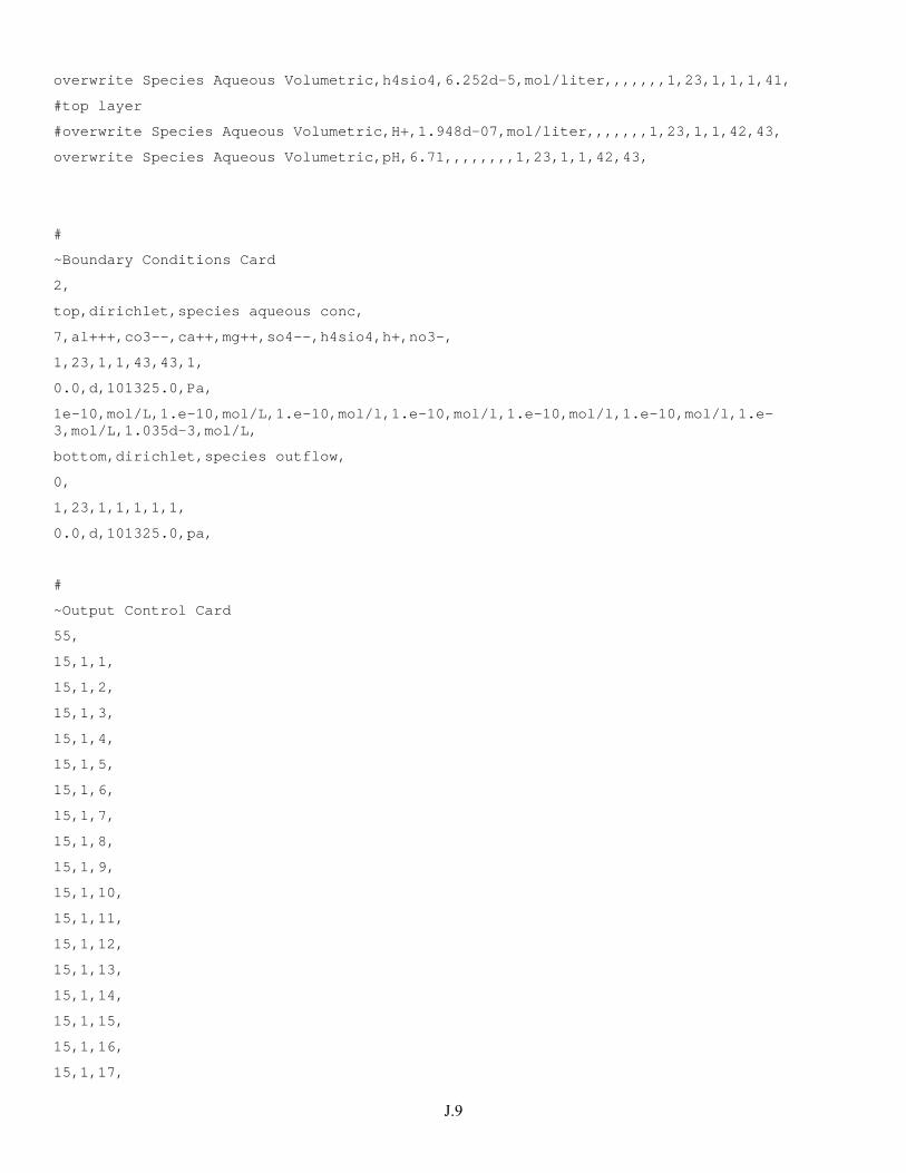
J.9
overwrite Species Aqueous Volumetric,h4sio4,6.252d-5,mol/liter,,,,,,,1,23,1,1,1,41,
#top layer
#overwrite Species Aqueous Volumetric,H+,1.948d-07,mol/liter,,,,,,,1,23,1,1,42,43,
overwrite Species Aqueous Volumetric,pH,6.71,,,,,,,,1,23,1,1,42,43,
#
~Boundary Conditions Card
2,
top,dirichlet,species aqueous conc,
7,al+++,co3--,ca++,mg++,so4--,h4sio4,h+,no3-,
1,23,1,1,43,43,1,
0.0,d,101325.0,Pa,
1e-10,mol/L,1.e-10,mol/L,1.e-10,mol/l,1.e-10,mol/l,1.e-10,mol/l,1.e-10,mol/l,1.e-3,mol/L,1.035d-3,mol/L,
bottom,dirichlet,species outflow,
0,
1,23,1,1,1,1,1,
0.0,d,101325.0,pa,
#
~Output Control Card
55,
15,1,1,
15,1,2,
15,1,3,
15,1,4,
15,1,5,
15,1,6,
15,1,7,
15,1,8,
15,1,9,
15,1,10,
15,1,11,
15,1,12,
15,1,13,
15,1,14,
15,1,15,
15,1,16,
15,1,17,
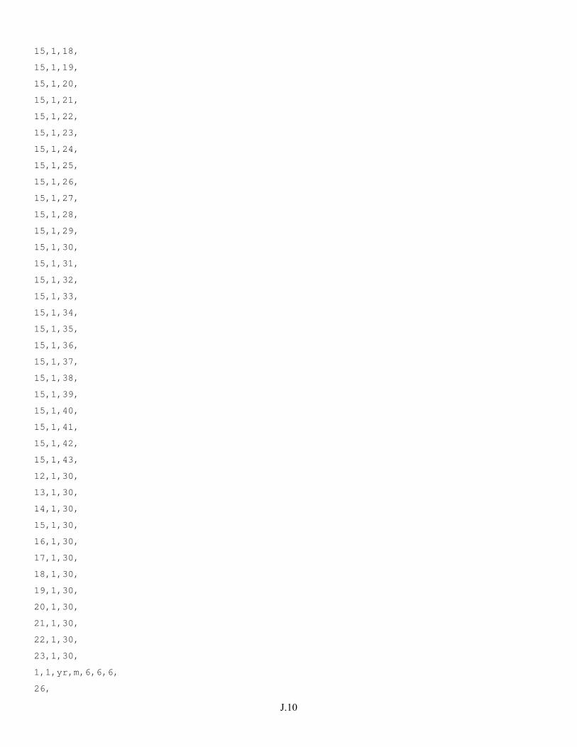
J.10
15,1,18,
15,1,19,
15,1,20,
15,1,21,
15,1,22,
15,1,23,
15,1,24,
15,1,25,
15,1,26,
15,1,27,
15,1,28,
15,1,29,
15,1,30,
15,1,31,
15,1,32,
15,1,33,
15,1,34,
15,1,35,
15,1,36,
15,1,37,
15,1,38,
15,1,39,
15,1,40,
15,1,41,
15,1,42,
15,1,43,
12,1,30,
13,1,30,
14,1,30,
15,1,30,
16,1,30,
17,1,30,
18,1,30,
19,1,30,
20,1,30,
21,1,30,
22,1,30,
23,1,30,
1,1,yr,m,6,6,6,
26,
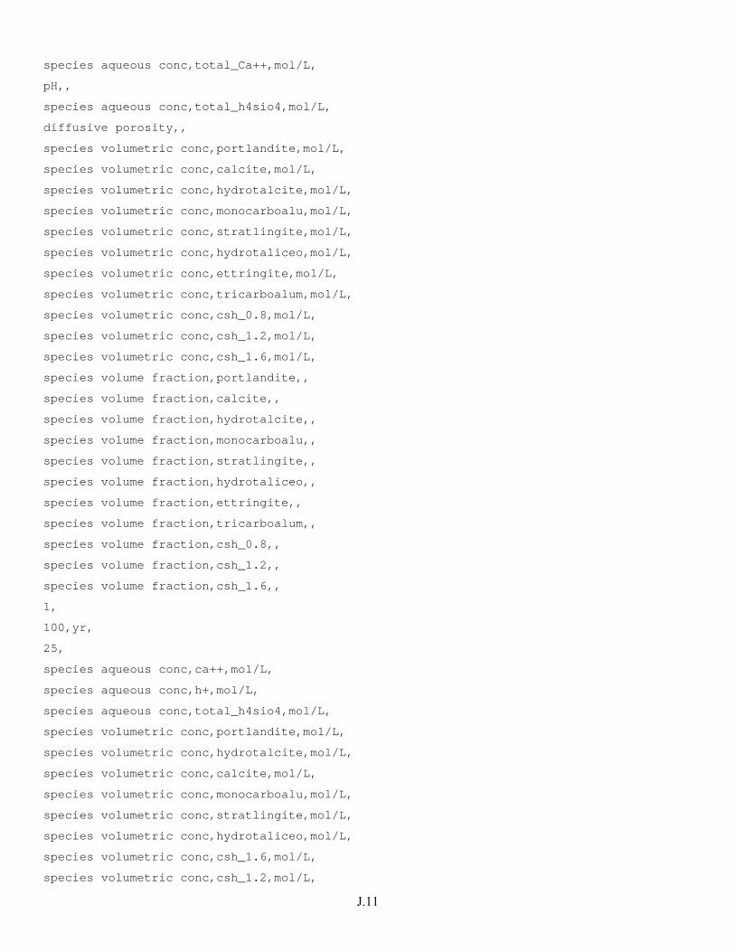
J.11
species aqueous conc,total_Ca++,mol/L,
pH,,
species aqueous conc,total_h4sio4,mol/L,
diffusive porosity,,
species volumetric conc,portlandite,mol/L,
species volumetric conc,calcite,mol/L,
species volumetric conc,hydrotalcite,mol/L,
species volumetric conc,monocarboalu,mol/L,
species volumetric conc,stratlingite,mol/L,
species volumetric conc,hydrotaliceo,mol/L,
species volumetric conc,ettringite,mol/L,
species volumetric conc,tricarboalum,mol/L,
species volumetric conc,csh_0.8,mol/L,
species volumetric conc,csh_1.2,mol/L,
species volumetric conc,csh_1.6,mol/L,
species volume fraction,portlandite,,
species volume fraction,calcite,,
species volume fraction,hydrotalcite,,
species volume fraction,monocarboalu,,
species volume fraction,stratlingite,,
species volume fraction,hydrotaliceo,,
species volume fraction,ettringite,,
species volume fraction,tricarboalum,,
species volume fraction,csh_0.8,,
species volume fraction,csh_1.2,,
species volume fraction,csh_1.6,,
1,
100,yr,
25,
species aqueous conc,ca++,mol/L,
species aqueous conc,h+,mol/L,
species aqueous conc,total_h4sio4,mol/L,
species volumetric conc,portlandite,mol/L,
species volumetric conc,hydrotalcite,mol/L,
species volumetric conc,calcite,mol/L,
species volumetric conc,monocarboalu,mol/L,
species volumetric conc,stratlingite,mol/L,
species volumetric conc,hydrotaliceo,mol/L,
species volumetric conc,csh_1.6,mol/L,
species volumetric conc,csh_1.2,mol/L,
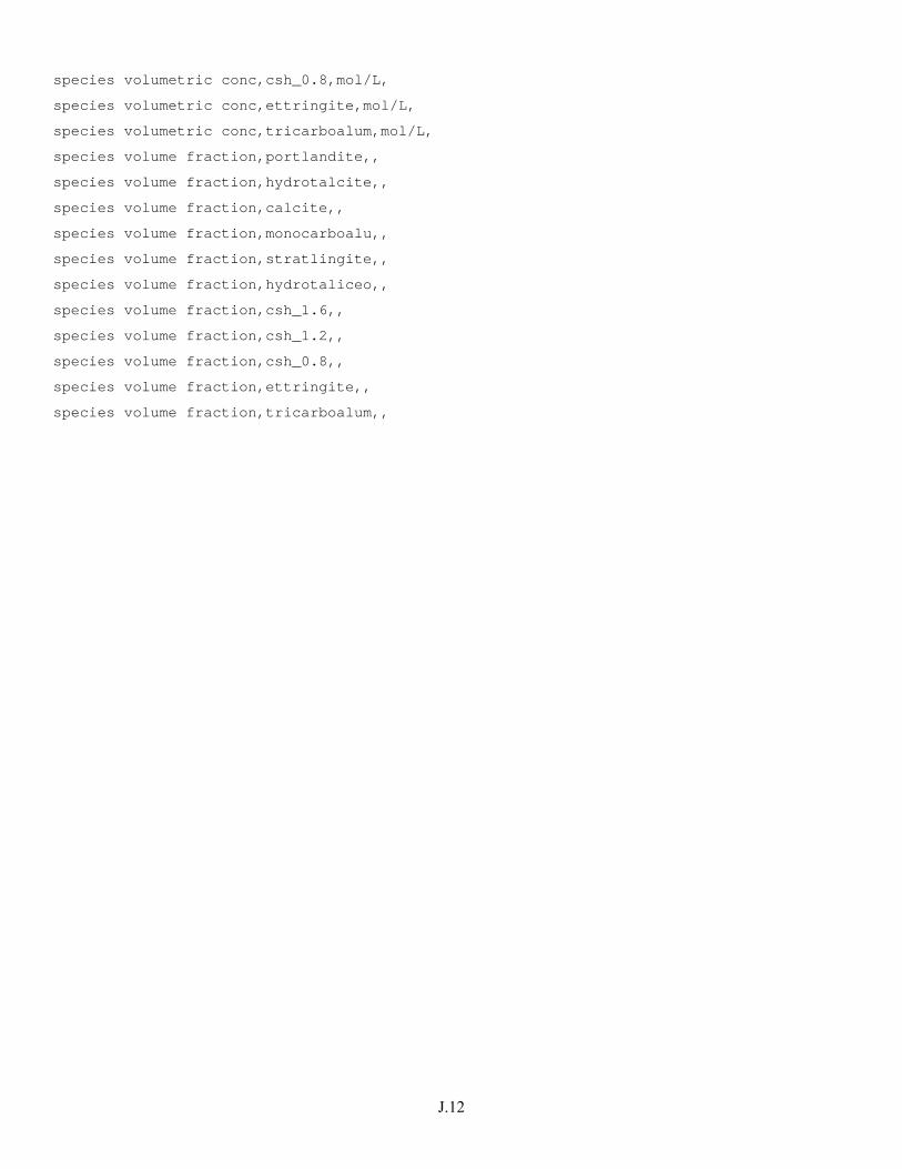
J.12
species volumetric conc,csh_0.8,mol/L,
species volumetric conc,ettringite,mol/L,
species volumetric conc,tricarboalum,mol/L,
species volume fraction,portlandite,,
species volume fraction,hydrotalcite,,
species volume fraction,calcite,,
species volume fraction,monocarboalu,,
species volume fraction,stratlingite,,
species volume fraction,hydrotaliceo,,
species volume fraction,csh_1.6,,
species volume fraction,csh_1.2,,
species volume fraction,csh_0.8,,
species volume fraction,ettringite,,
species volume fraction,tricarboalum,,
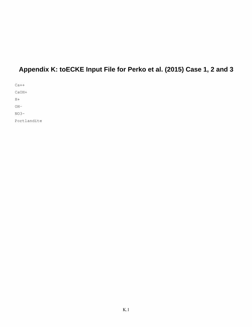
K.1
Appendix K: toECKE Input File for Perko et al. (2015) Case 1, 2 and 3
Ca++
CaOH+
H+
OH-
NO3-
Portlandite
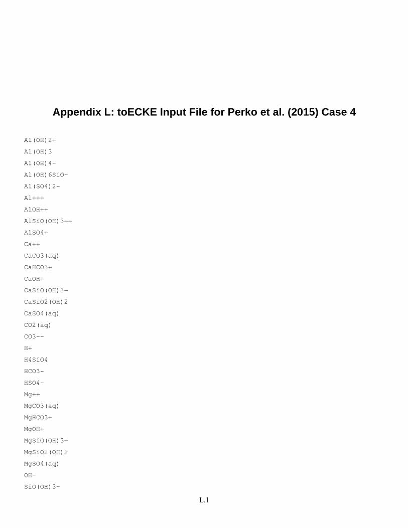
L.1
Appendix L: toECKE Input File for Perko et al. (2015) Case 4
Al(OH)2+
Al(OH)3
Al(OH)4-
Al(OH)6SiO-
Al(SO4)2-
Al+++
AlOH++
AlSiO(OH)3++
AlSO4+
Ca++
CaCO3(aq)
CaHCO3+
CaOH+
CaSiO(OH)3+
CaSiO2(OH)2
CaSO4(aq)
CO2(aq)
CO3--
H+
H4SiO4
HCO3-
HSO4-
Mg++
MgCO3(aq)
MgHCO3+
MgOH+
MgSiO(OH)3+
MgSiO2(OH)2
MgSO4(aq)
OH-
SiO(OH)3-
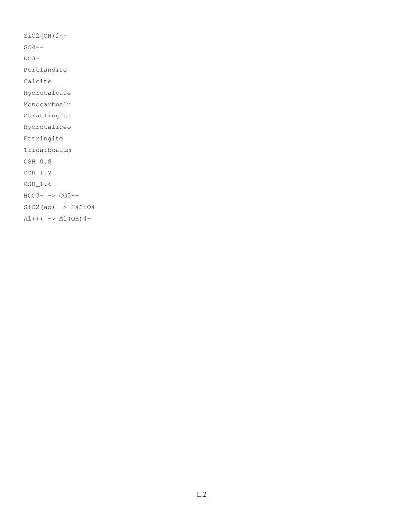
L.2
SiO2(OH)2--
SO4--
NO3-
Portlandite
Calcite
Hydrotalcite
Monocarboalu
Stratlingite
Hydrotaliceo
Ettringite
Tricarboalum
CSH_0.8
CSH_1.2
CSH_1.6
HCO3- -> CO3--
SiO2(aq) -> H4SiO4
Al+++ -> Al(OH)4-

L.1
RPT-IGTP-010 Rev. 0
Distribution*
No. of No. of Copies Copies
Distr. 1
OFFSITE Oak Ridge National Laboratory EM Pierce U.S. Department of Energy Office of River Protection AA Kruger GL Pyles Washington River Protection Solutions EE Brown PA Cavanah SE Kelly KP Lee (AREVA) WG Ramsey KH Subramanian DJ Swanberg LE Thompson Savannah River National Laboratory AD Cozzi GP Flach KM Fox CC Herman CM Jantzen Vitreous State Laboratory H Gan W Kot I Muller IL Pegg Energy Solutions I Joseph Intera R Andrews *All electronic distributions.
ONSITE Pacific Northwest National Laboratory DH Bacon SD Burton VL Freedman SN Kerisit JJ Neeway DK Peeler ML Rockhold JV Ryan RJ Serne GL Smith MM Valenta JD Vienna JH Westsik, Jr.


Related Documents