Iipm chapter 3

Advanced Excel – Version 1.2 Updated Jan 10, 2010 - IIPM

All rights reserved. Material Designed by Rahul Kumar Kandoi.

Chapter

3

Excel Tools

Conditional Formatting

If a cell contains formula results or other cell values that you want to monitor, you can identify the cells by applying conditional formats. For example, you can apply green shading (highlighting) to

the cell if the sales exceed forecast and red shading if sales fall short.

Select the cells to be formatted.

On the Format menu, click Conditional Formatting. On the conditional formatting window, select the condition you want to set for the values in the cells. To change formats, click Format for the condition you want to change. To reselect formats on the current tab of the Format Cells dialog box, click Clear.



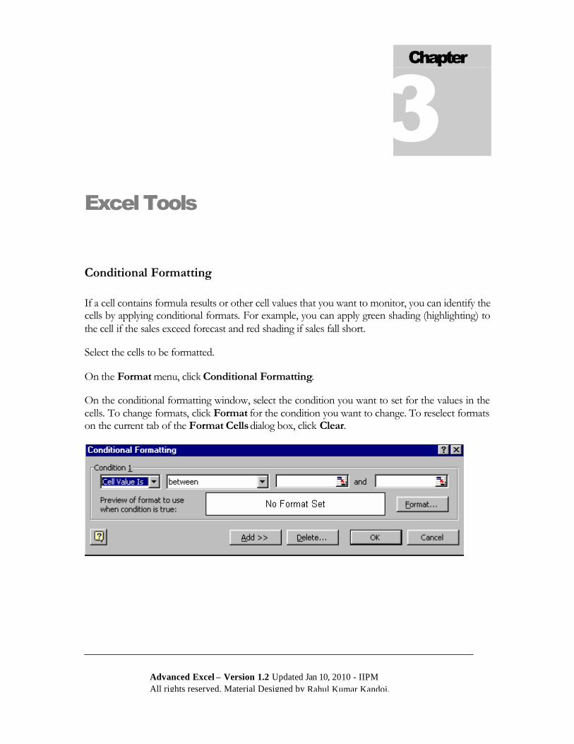
Select the Font Style, Color, Underline, and Strikethrough from the Font Tab.

From the Border Tab, select if border is needed, kind of Border, Color of Border.



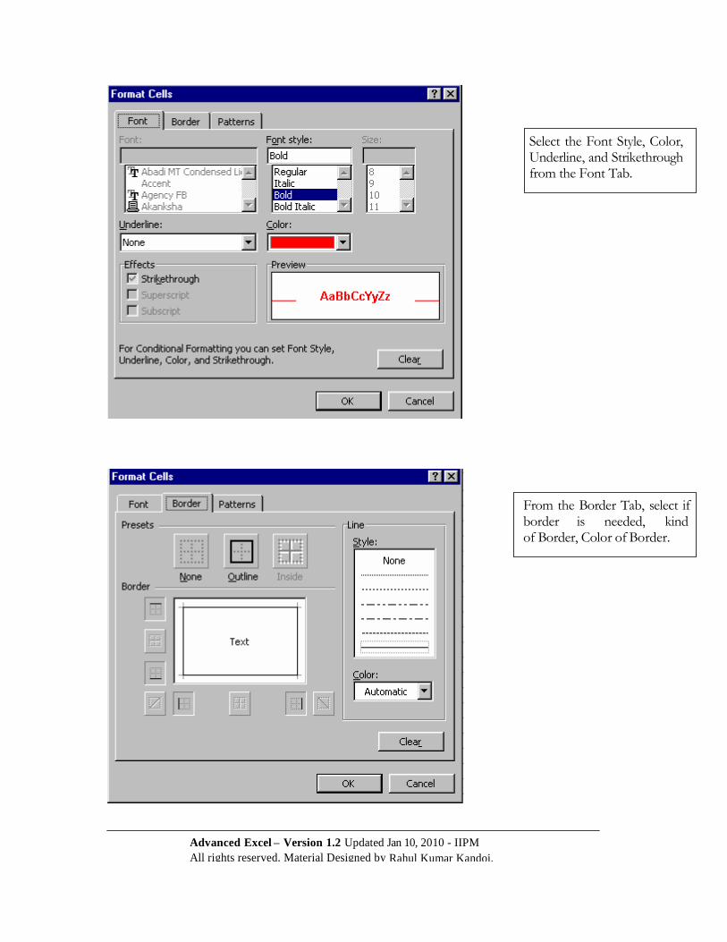
Click on the Pattern Tab to select background and Pattern of Fill.

This is what the Conditional Formatting Window appears like after setting the format.

To add a new condition, click Add.

To remove one or more conditions, click Delete on the condition you want to delete.



H Hyperlink

yperlink creates a shortcut or jump that opens a document stored on a network

server, an intranet, or the Internet. When you click the cell that contains the

HYPERLINK function, Microsoft Excel opens the file stored at link_location.

Create a hyperlink to an existing file

1. Right-click the text or graphic you want to represent the hyperlink, and then click

Hyperlink on the shortcut menu.

2. Under Link to, click Existing file or Web page.

3. Do one of the following:

To select the file from a list of files you have recently used, click Recent Files

and then click the file you want to link to.

4. To select the file from a list of existing files, click the File button under Browse

for, and then locate and double-click the file you want to link to.

5. To assign a tip to be displayed when you rest the pointer on the hyperlink, click

ScreenTip and then type the text you want in the ScreenTip text box. Click O K.

Create a hyperlink to a Web page

1. Right-click the text or graphic you want to represent the hyperlink, and then click

Hyperlink on the shortcut menu.

2. Under Link to, click Existing file or Web page.

3. Do one of the following:

To select the Web page from a list of Web pages you have recently browsed, click

Browsed Pages and then click the Web page you want to link to.

To select the Web page by openi ng your browser and searching for the page, click

the Web Page button under Browse for, open the Web page you want to link to,

and then switch back to Microsoft Excel without closing your browser.

4. To assign a tip to be displayed when you rest the pointer on the hyperlink, click

ScreenTip and then type the text you want in the ScreenTip text box. Click O K



Filter

Filtering is a quick and easy way to find and work with a subset of data in a list. A

filtered list displays only the rows that meet the criteria you specify for a column.

Microsoft Excel provides two commands for filtering lists:

AutoFilter, which includes filter by selection, for simple criteria

Advanced Filter, for more complex criteria

Unlike sorting, filtering does not rearrange a list. Filtering temporarily hides rows you do

not want displayed.

When Excel filters rows, you can edit, format, chart, and print your list subset without

rearranging or moving it.

Auto Filter

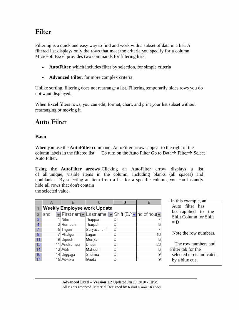
Basic When you use the AutoFilter command, AutoFilter arrows appear to the right of the

column labels in the filtered list. To turn on the Auto Filter Go to Data Filter Select

Auto Filter. Using the AutoFilter arrows Clicking an AutoFilter arrow displays a list

of all unique, visible items in the column, including blanks (all spaces) and

nonblanks. By selecting an item from a list for a specific column, you can instantly

hide all rows that don't contain

the selected value.

In this example, an

Auto filter has been applied to the

Shift Column for Shift = D

Note the row numbers.

The row numbers and

Filter tab for the selected tab is indicated

by a blue cue.



Quickly filtering values If you are filtering a list of numbers, you can quickly view the

largest values in the list by clicking the Top 10 item in the AutoFilter list. To resume

viewing everything in the column, click All. Viewing a filtered list Microsoft Excel indicates the filtered items with some visual

cues.

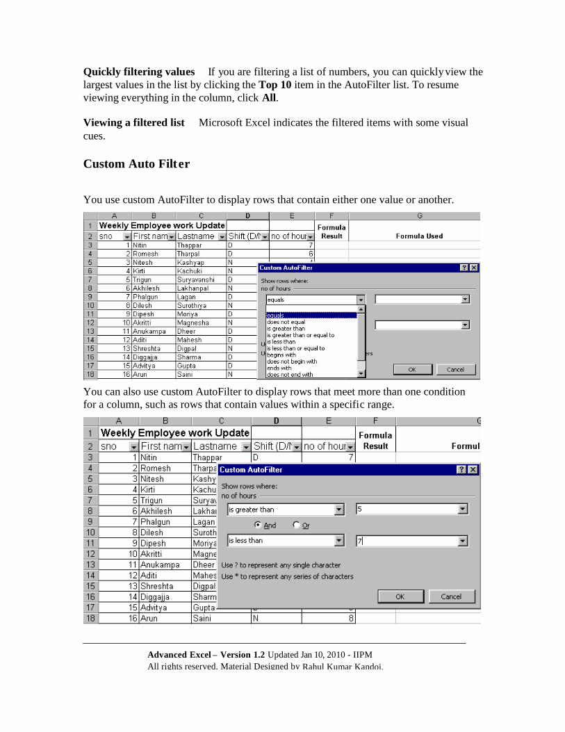
Custom Auto Filt er

You use custom AutoFilter to display rows that contain either one value or another.

You can also use custom AutoFilter to display rows that meet more than one condition

for a column, such as rows that contain values within a specific range.



Advanced Filter

As the name suggests, Advanced Filter is a step ahead of the Basic Filter. Advanced

filter criteria can include multiple conditions applied in a single column, multiple criteria

applied to multiple columns, and conditions created as the result of a formula.

Filter a list by using advanced criteria

Your worksheet should have at least three blank rows above the list that can be used as a

criteria range. The list must have column labels.

1. Select the column labels from the list for the columns that contain the values you want to

filter, and click Copy

2. Select the first blank row of the criteria range, and click Paste

3. In the rows below the criteria labels, type the criteria you want to match. Make

sure there is at least one blank row between the criteria values and the list.

4. Click a cell in the list.

5. On the Data menu, point to Filter, and then click Advanced Filter.

6. To filter the list by hiding rows that don't match your criteria, click Filter the list,

in-place.

7. To filter the list by copying rows that match your criteria to another area of

the worksheet, click Copy to another location, click in the Copy to box, and

then click the upper-left corner of the area where you want to paste the rows.

8. In the Criteria range box, enter the reference for the criteria range, including the

criteria labels.

9. To move the Advanced Filter dialog box out of the way temporarily while you

select the criteria range, click Collapse Dialog



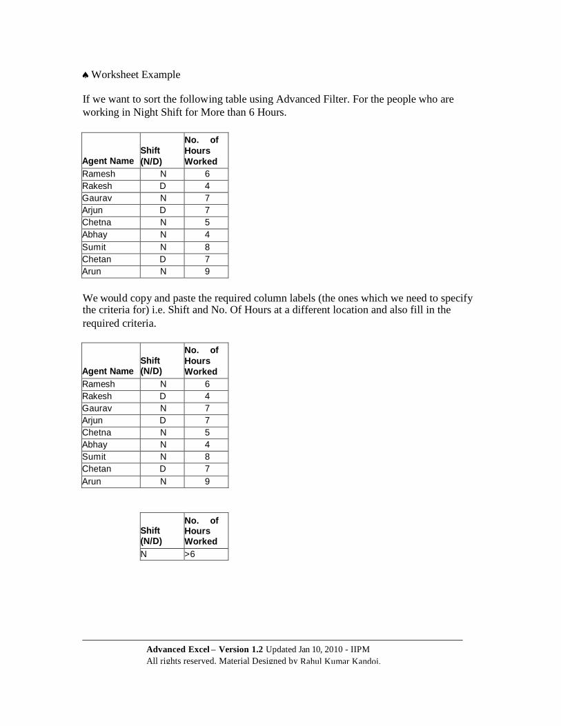
Worksheet Example If we want to sort the following table using Advanced Filter. For the people who are

working in Night Shift for More than 6 Hours.

Agent Name

Shift

(N/D)

No. of

Hours

Worked Ramesh N 6 Rakesh D 4 Gaurav N 7 Arjun D 7 Chetna N 5 Abhay N 4

Sumit N 8 Chetan D 7 Arun N 9

We would copy and paste the required column labels (the ones which we need to specify the criteria for) i.e. Shift and No. Of Hours at a different location and also fill in the

required criteria.

Agent Name

Shift (N/D)

No. of

Hours Worked

Ramesh N 6 Rakesh D 4 Gaurav N 7 Arjun D 7 Chetna N 5 Abhay N 4 Sumit N 8 Chetan D 7

Arun N 9

Shift (N/D)

No. of Hours Worked

N >6



__________________________

___________________________

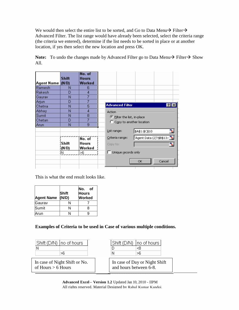
We would then select the entire list to be sorted, and Go to Data Menu Filter

Advanced Filter. The list range would have already been selected, select the criteria range

(the criteria we entered), determine if the list needs to be sorted in place or at another

location, if yes then select the new location and press OK.

Note: To undo the changes made by Advanced Filter go to Data Menu Filter Show

All.

This is what the end result looks like.

Agent Name

Shift (N/D)

No. of Hours Worked

Gaurav N 7 Sumit N 8

Arun N 9

Examples of Criteria to be used in Case of various multiple conditions.

In case of Night Shift or No. of Hours > 6 Hours

In case of Day or Night Shift and hours between 6-8.

_



Sorting Data

Default Sort Orders

Microsoft Excel uses specific sort orders to arrange data according to the value, not the

format, of the data.

In an ascending sort, Excel uses the following order. (In a descending sort, this sort order

is reversed except for blank cells, which are always placed last.)

Numbers Numbers are sorted from the smallest negative number to the largest positive

number.

Alphanumeric sort When you sort alphanumeric text, Excel sorts left to right, character

by character. For example, if a cell contains the text "A100," Excel places the cell after a

cell that contains the entry "A1" and before a cell that contains the entry "A11."

Text and text that includes numbers are sorted in the following order:

0 1 2 3 4 5 6 7 8 9 (space) ! " # $ % & ( ) * , . / : ; ? @ [ \ ] ^ _ ` { | } ~ + < = > A B C D E

F G H I J K L M N O P Q R S T U V W X Y Z Apostrophes (') and hyphens (-) are ignored, with one exception: If two text strings are

the same except for a hyphen, the text with the hyphen is sorted last.

Logical values In logical values, FALSE is placed before TRUE.

Error values All error values are equal.

Blanks Blanks are always placed last.

Sort Data

1. Click a cell in the list you want to sort.

2. On the Data menu, click Sort.

3. Click Options to choose Orientation of the data you want to sort. (Default is top to bottom)

4. In the Sort by and Then by boxes, click the way you want to sort your data.



Worksheet Example

Result:



Subtotals

Microsoft Excel can automatically summarize data by calculating subtotal and grand total

values in a list. To use automatic subtotals, your list must contain labeled columns and

and the list must be sorted on the columns for which you want subtotals. When you insert automatic subtotals, Excel outlines the list by grouping detail rows with

each associated subtotal row, and grouping subtotal rows with the grand total row. You

can choose the function for Excel to use when it calculates totals.

Insert Subtotals in a list.

1. Sort the list by the column for which you want to calculate subtotals. For

example, to summarize the units sold by each salesperson in a list of salespeople, sales amounts, and the number of units sold, sort the list by the salesperson

column.

2. Click a cell in the list.

3. On the Data menu, click Subtotals.

Page 14 of 29

________________________________________________

Advanced Excel – Version 1.1 Nov

Convergys Corporation, Company confidential. All rights re

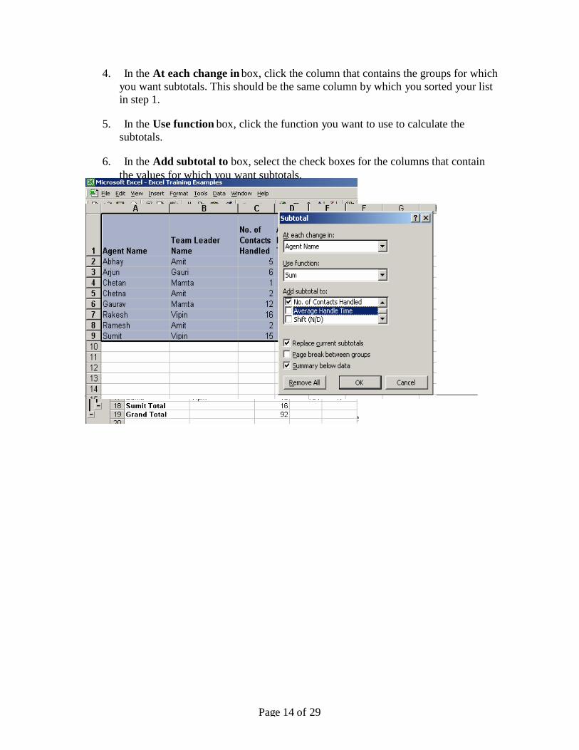
4. In the At each change in box, click the column that contains the groups for which

you want subtotals. This should be the same column by which you sorted your list

in step 1.

5. In the Use function box, click the function you want to use to calculate the

subtotals.

6. In the Add subtotal to box, select the check boxes for the columns that contain

the values for which you want subtotals.

Page 15 of 29

_________________________________________________________

Advanced Excel – Version 1.1 Nov 5, 2002

Group and Outline

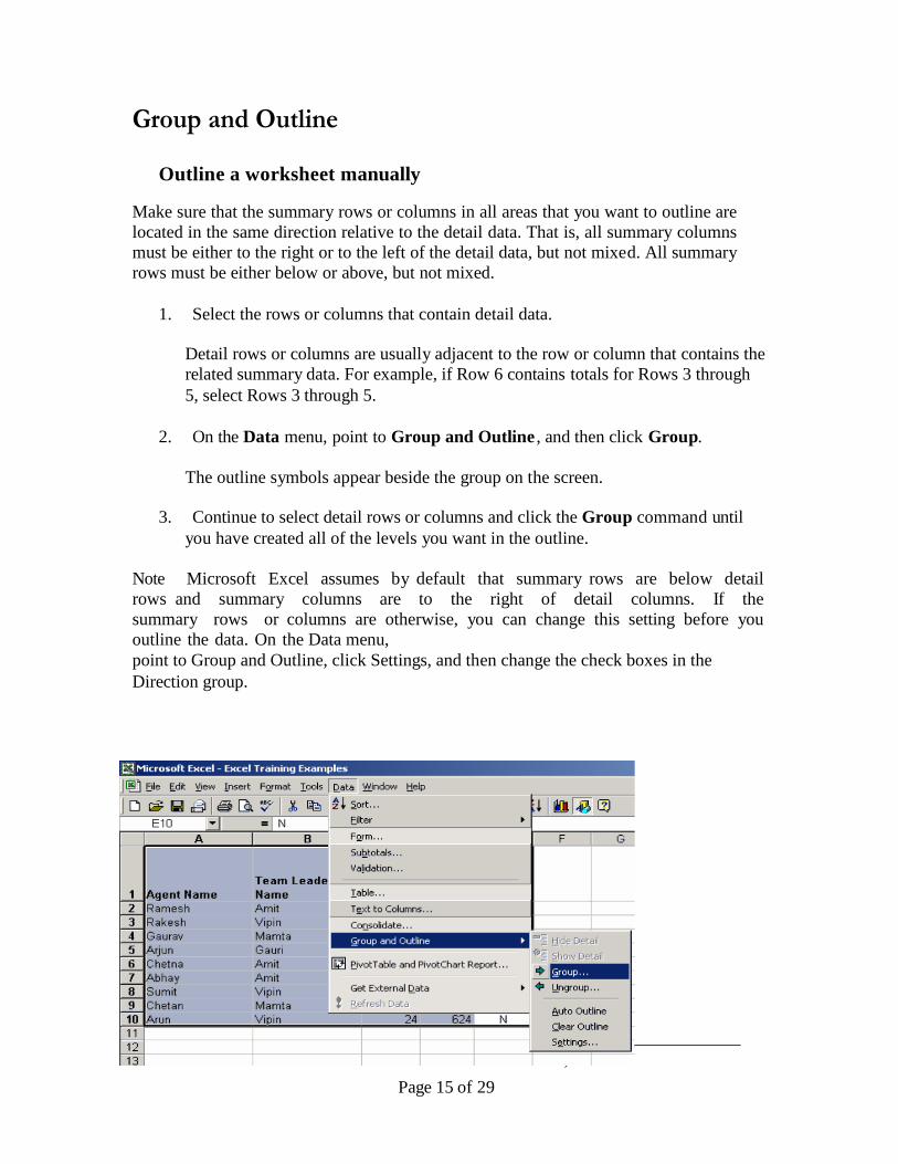
Outline a worksheet manually

Make sure that the summary rows or columns in all areas that you want to outline are

located in the same direction relative to the detail data. That is, all summary columns

must be either to the right or to the left of the detail data, but not mixed. All summary

rows must be either below or above, but not mixed.

1. Select the rows or columns that contain detail data.

Detail rows or columns are usually adjacent to the row or column that contains the

related summary data. For example, if Row 6 contains totals for Rows 3 through

5, select Rows 3 through 5.

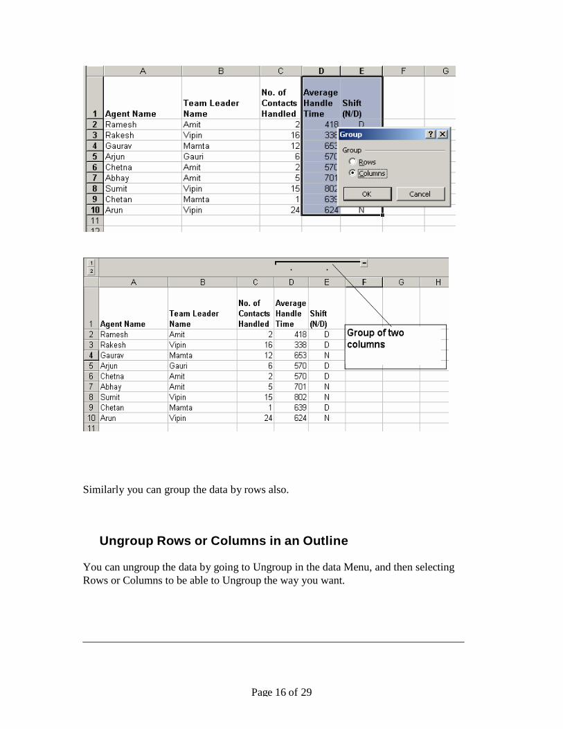
2. On the Data menu, point to Group and Outline , and then click Group.

The outline symbols appear beside the group on the screen.

3. Continue to select detail rows or columns and click the Group command until

you have created all of the levels you want in the outline.

Note Microsoft Excel assumes by default that summary rows are below detail

rows and summary columns are to the right of detail columns. If the

summary rows or columns are otherwise, you can change this setting before you

outline the data. On the Data menu,

point to Group and Outline, click Settings, and then change the check boxes in the

Direction group.

Page 16 of 29

Similarly you can group the data by rows also.

Ungroup Rows or Columns in an Outline You can ungroup the data by going to Ungroup in the data Menu, and then selecting

Rows or Columns to be able to Ungroup the way you want.

Page 17 of 29

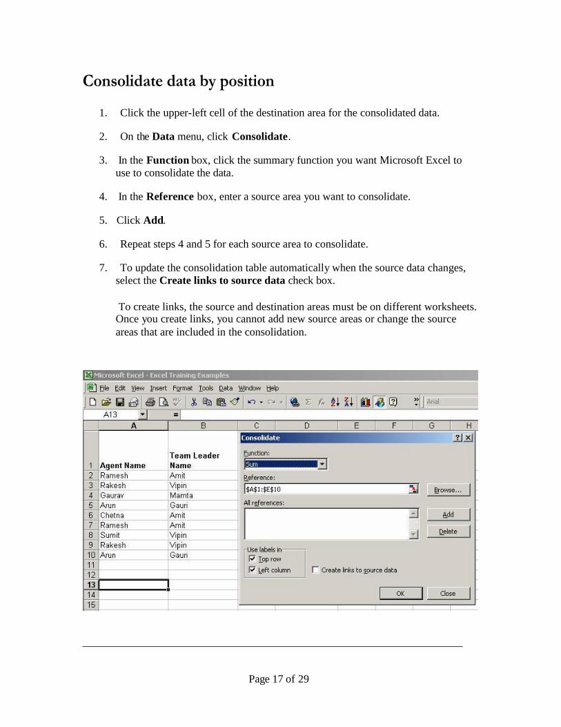
Consolidate data by position

1. Click the upper-left cell of the destination area for the consolidated data.

2. On the Data menu, click Consolidate.

3. In the Function box, click the summary function you want Microsoft Excel to

use to consolidate the data.

4. In the Reference box, enter a source area you want to consolidate.

5. Click Add.

6. Repeat steps 4 and 5 for each source area to consolidate.

7. To update the consolidation table automatically when the source data changes,

select the Create links to source data check box.

To create links, the source and destination areas must be on different worksheets. Once you create links, you cannot add new source areas or change the source

areas that are included in the consolidation.

Page 18 of 29

What If Analysis Tools

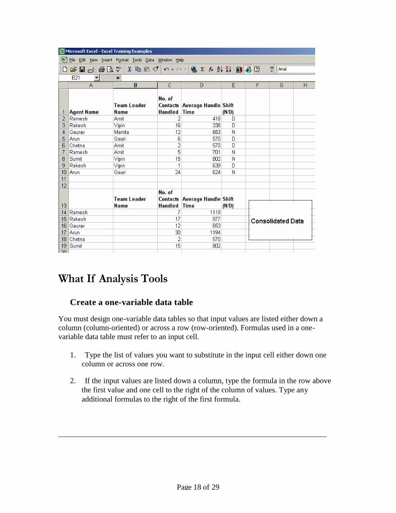
Create a one-variable data table

You must design one-variable data tables so that input values are listed either down a

column (column-oriented) or across a row (row-oriented). Formulas used in a one-

variable data table must refer to an input cell.

1. Type the list of values you want to substitute in the input cell either down one

column or across one row.

2. If the input values are listed down a column, type the formula in the row above

the first value and one cell to the right of the column of values. Type any

additional formulas to the right of the first formula.

Page 19 of 29

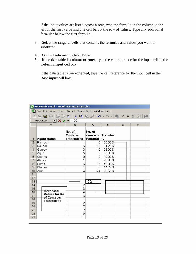
If the input values are listed across a row, type the formula in the column to the

left of the first value and one cell below the row of values. Type any additional

formulas below the first formula.

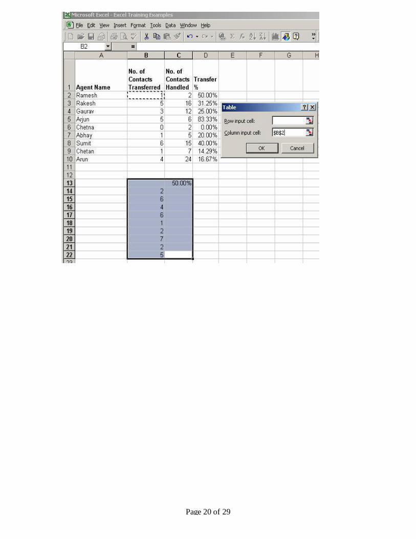
3. Select the range of cells that contains the formulas and values you want to

substitute.

4. On the Data menu, click Table .

5. If the data table is column-oriented, type the cell reference for the input cell in the

Column input cell box.

If the data table is row -oriented, type the cell reference for the input cell in the

Row input cell box.

Page 20 of 29

Page 21 of 29

_____________________________________________________________________

Create a two-variable data table

Two-variable data tables use only one formula with two lists of input values. The formula

must refer to two different input cells.

1. In a cell on the worksheet, enter the formula that refers to the two input cells.

2. Type one list of input values in the same column, below the formula. Type the

second list in the same row, to the right of the formula.

3. Select the range of cells that contains the formula and both the row and column of

values.

4. On the Data menu, click Table .

5. In the Row input cell box, enter the reference for the input cell for the input

values in the row.

6. In the Column input cell box, enter the reference for the input cell for the input

values in the column.

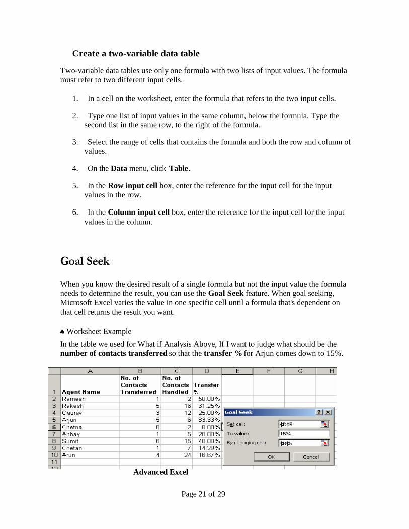
Goal Seek

When you know the desired result of a single formula but not the input value the formula

needs to determine the result, you can use the Goal Seek feature. When goal seeking,

Microsoft Excel varies the value in one specific cell until a formula that's dependent on

that cell returns the result you want.

Worksheet Example

In the table we used for What if Analysis Above, If I want to judge what should be the

number of contacts transferred so that the transfer % for Arjun comes down to 15%.

Advanced Excel

Page 22 of 29

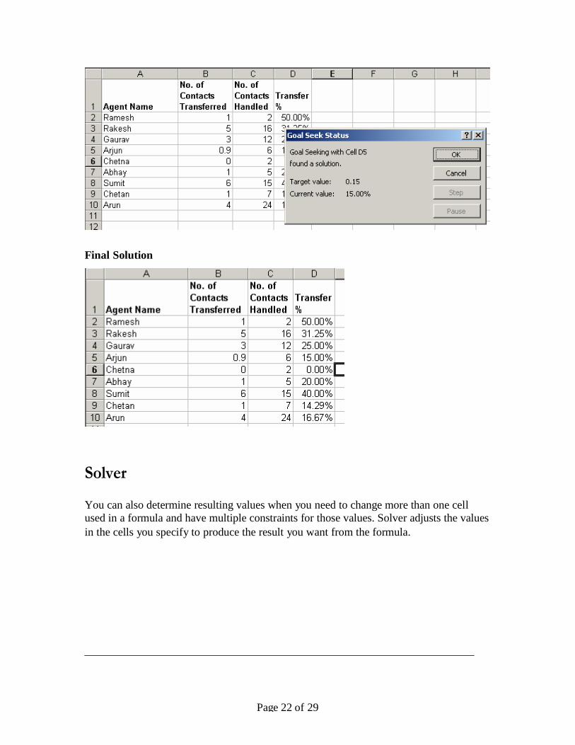
Final Solution

Solver

You can also determine resulting values when you need to change more than one cell

used in a formula and have multiple constraints for those values. Solver adjusts the values

in the cells you specify to produce the result you want from the formula.

Page 23 of 29

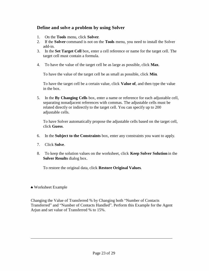
Define and solve a problem by using Solver

1. On the Tools menu, click Solver.

2. If the Solver command is not on the Tools menu, you need to install the Solver add-in.

3. In the Set Target Cell box, enter a cell reference or name for the target cell. The

target cell must contain a formula.

4. To have the value of the target cell be as large as possible, click Max.

To have the value of the target cell be as small as possible, click Min.

To have the target cell be a certain value, click Value of, and then type the value

in the box.

5. In the By Changing Cells box, enter a name or reference for each adjustable cell,

separating nonadjacent references with commas. The adjustable cells must be

related directly or indirectly to the target cell. You can specify up to 200

adjustable cells.

To have Solver automatically propose the adjustable cells based on the target cell,

click Guess.

6. In the Subject to the Constraints box, enter any constraints you want to apply.

7. Click Solve.

8. To keep the solution values on the worksheet, click Keep Solver Solution in the

Solver Results dialog box.

To restore the original data, click Restore Original Values.

Worksheet Example

Changing the Value of Transferred % by Changing both “Number of Contacts

Transferred” and “Number of Contacts Handled”. Perform this Example for the Agent

Arjun and set value of Transferred % to 15%.

Page 24 of 29

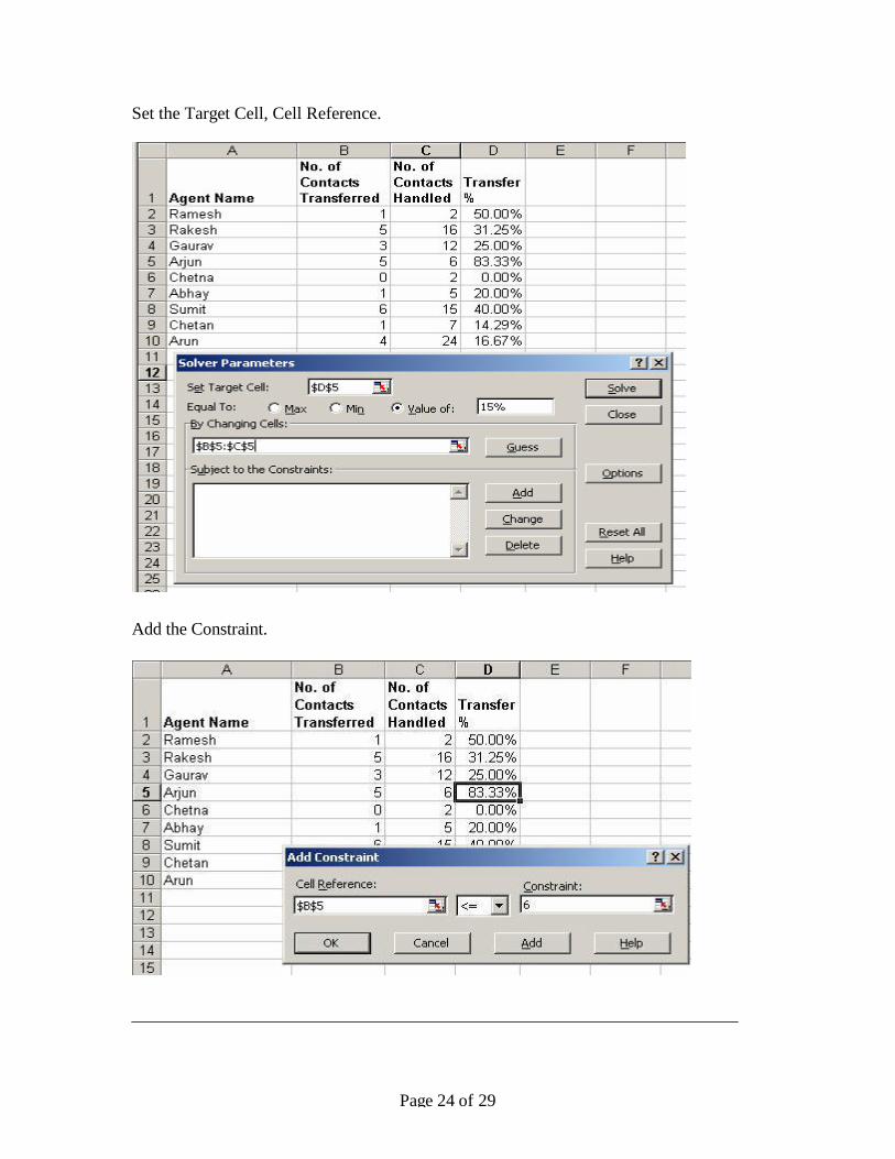
Set the Target Cell, Cell Reference.

Add the Constraint.

Page 25 of 29

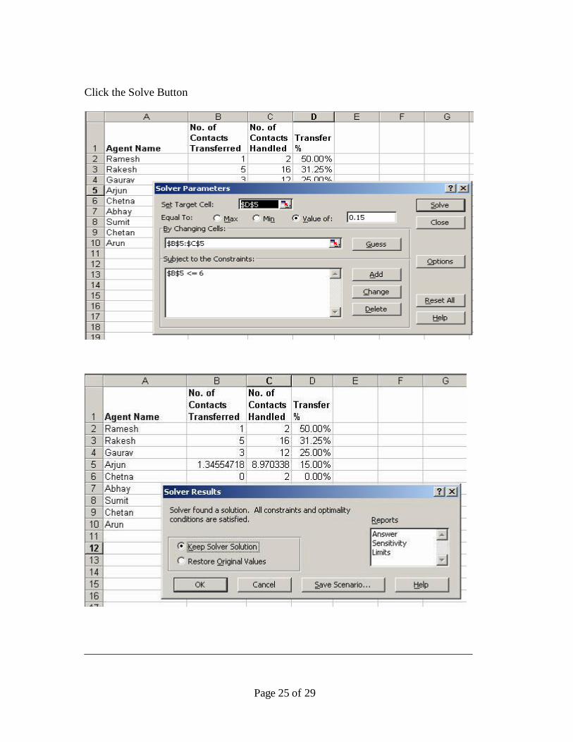
Click the Solve Button

Page 26 of 29

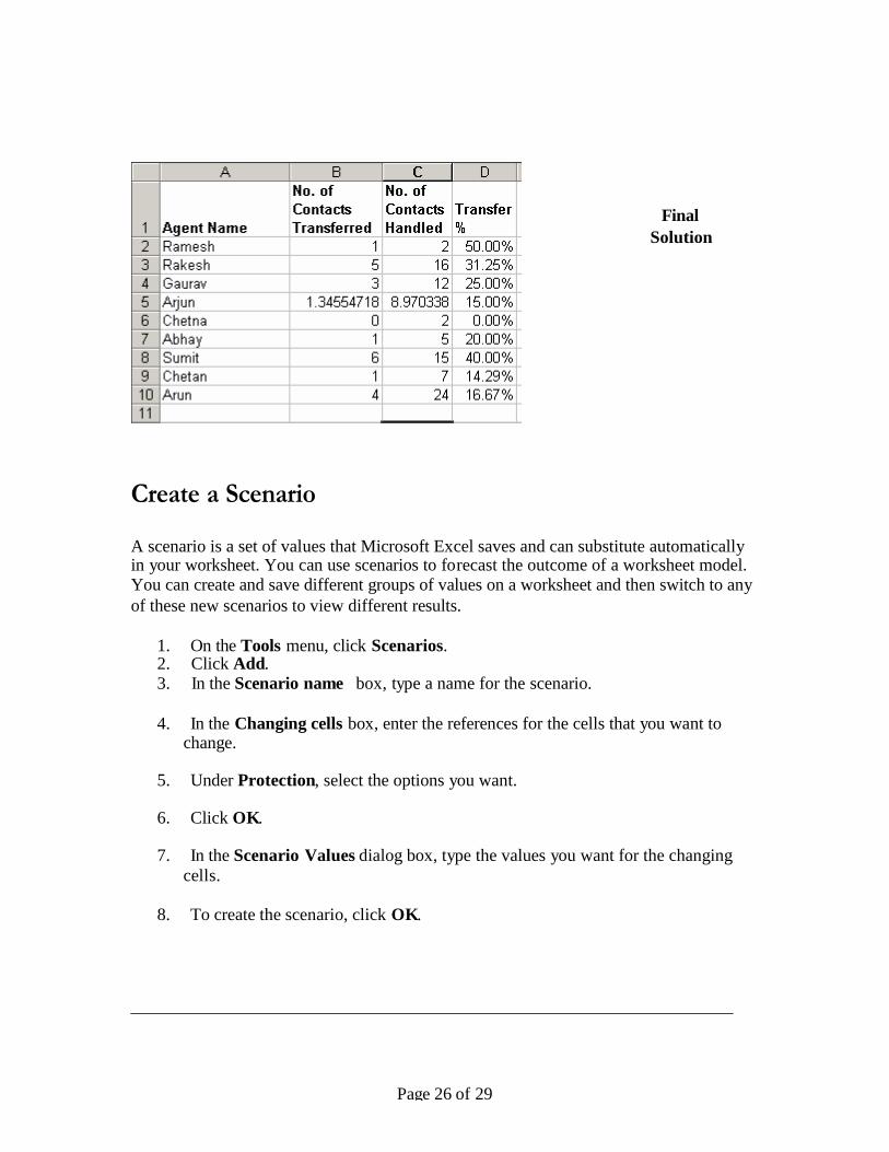
Create a Scenario

Final

Solution

A scenario is a set of values that Microsoft Excel saves and can substitute automatically in your worksheet. You can use scenarios to forecast the outcome of a worksheet model. You can create and save different groups of values on a worksheet and then switch to any

of these new scenarios to view different results.

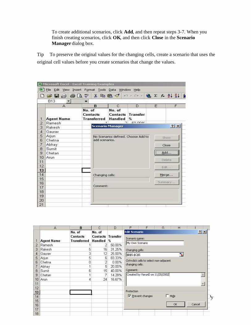
1. On the Tools menu, click Scenarios. 2. Click Add. 3. In the Scenario name box, type a name for the scenario.

4. In the Changing cells box, enter the references for the cells that you want to change.

5. Under Protection, select the options you want.

6. Click OK.

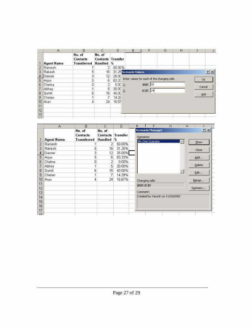
7. In the Scenario Values dialog box, type the values you want for the changing

cells.

8. To create the scenario, click OK.

_____________________________________________________________________

Advanced Excel – Version 1.1 Nov 5, 2002

Convergys Corporation, Company confidential. All rights reserved. Material Designed b Varun Dhamija.

Page 26 of 29

To create additional scenarios, click Add, and then repeat steps 3-7. When you

finish creating scenarios, click OK, and then click Close in the Scenario

Manager dialog box.

Tip To preserve the original values for the changing cells, create a scenario that uses the

original cell values before you create scenarios that change the values.

y

Page 27 of 29

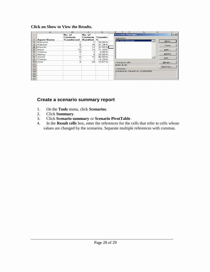
Click on Show to View the Results.

Create a scenario summary report

1. On the Tools menu, click Scenarios.

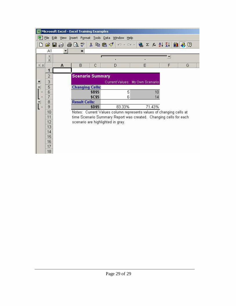
2. Click Summary. 3. Click Scenario summary or Scenario PivotTable . 4. In the Result cells box, enter the references for the cells that refer to cells whose

values are changed by the scenarios. Separate multiple references with commas.

Page 28 of 29

Page 29 of 29

Iipm chapter 3

Documents