Ift 2421 Chapitre 4 Interpolation polynomiale : Collocation

Ift2421 1 Chapitre 4

Ift 2421

Chapitre 4

Interpolationpolynomiale :Collocation

Ift2421 2 Chapitre 4

Introduction

Lancement d'une fusée.Déterminer la trajectoire avec précision.

La position n'est alors connue qu'en fonction d'un certainnombre de points d'abscisses fixes.

Le problème consiste à évaluer cette fonctionailleurs qu'aux points donnés.

Interpolation

Extrapolation

Ift2421 3 Chapitre 4

Linéarisation par morceaux

Droite entre deux pointsconsécutifs.

Méthode en généralimprécise.

Ift2421 4 Chapitre 4

Méthode de collocation

Trouver un polynômequi passe par tous les points donnés.

Avec (x0,f0), (x1,f1), (x2,f2), ... , (xn,fn) et xi ≠ xj

Il y a n+1 conditions.

Trouver le polynôme Pn(x) tel quePn(xi) = fi pour i = 0, 1, ... , n

Exemple :

2 points → droite y = ax + b(polynôme de degré 1)

3 points → paraboley = ax2 + bx +c

(polynôme de degré 2)

Remarque :

Quelque soit la méthode, lepolynôme de collocation sera

toujours le même.

Ift2421 5 Chapitre 4

Recherche de Pn(x) : première approche

Pn(x) est donné par :

Pn(x) = a0 + a1 x + a2 x2 + ... + an x

n

Le polynôme de collocation vérifie les n+1 conditions :

Pn(xi) = fi pour i = 0, 1 , ..., n.

Les n+1 coefficients a0, a1, ..., an sont donnéspar la résolution du système

de n+1 équations et n+1 inconnues :

Pn(x0) = a0 + a1 x0 + a2 x02 + ... + an x0

n

Pn(x1) = a0 + a1 x1 + a2 x12 + ... + an x1

n

...Pn(xn) = a0 + a1 xn + a2 xn

2 + ... + an xnn

Remarque :

Cette approche n’est pas un moyen pratique de calculer Pn(x).

Ift2421 6 Chapitre 4

Unicité du polynôme de collocation

théorème:

Le polynôme de collocation de degré nqui satisfait les n+1 conditionsPn( xi ) = fi pour i = 0, 1 , ..., n

est unique.

Preuve:

Supposons l'existence de deux polynômes de collocationPn et Qn qui satisfont les n+1 conditions

Pn(xi) = fi pour i = 0, 1 , ..., n.Qn(xi) = fi pour i = 0, 1 , ..., n.

D(x) = Pn(x) - Qn(x)est au plus de degré n.

D(xi) = Pn(xi) - Qn(xi) = fi - fi = 0

donc possède au moins n+1 racines : i = 0, 1 , ..., n.

Or un polynôme de degré n ne peut pas posséderplus de n racines.

La seule possibilité D = 0.Donc Pn = Qn

Ift2421 7 Chapitre 4

Existence du polynôme de collocation

1.Cas linéaire ( n = 1 )

Avec P0(x0,f0) et P1(x1,f1), 2 conditions

Cherchons P1(x) = a0 + a1 x

conditions de collocation:

P1(x0) = a0 + a1 x0 = f0

P1(x1) = a0 + a1 x1 = f1

Solution sous la forme

P xx x

x xf

x x

x xf1

1

0 10

0

1 01( )

( )

( )

( )

( )=

−−

+−−

⇒ polynôme de Lagrange de degré 1.

Note:

1

10

1

0

1

0

1

x

x

a

a

f

f

⋅

=

det(A) = (x1 - x0) ≠ 0 si x1 ≠ x0

⇒ A régulière⇒ Solution a0, a1 unique

⇒ P1(x) unique

Ift2421 8 Chapitre 4

Exemple:

Trouver le polynôme de collocationpassant par les deux points

xi : 1.0 4.0fi : 2.0 0.5

P xx x

1

4

1 42 0

1

4 10 5( )

( )

( ).

( )

( ).=

−−

+−−

P x x x1

2

3

8

3

1

6

1

6( ) = − + + −

P x x1

1

2

5

2( ) = − +

-1 1 2 3 4 5 6

-0.5

0.5

1

1.5

2

2.5

3

3.5

x1

x2

Ift2421 9 Chapitre 4

Existence du polynôme de collocation

2.Cas parabolique { n = 2 }

Avec (x0,f0), (x1,f1) et (x2,f2).

3 conditions

P2(x0) = a0 + a1 x0 + a2 x02 = f0

P2(x1) = a0 + a1 x1 + a2 x12 = f1

P2(x2) = a0 + a1 x2 + a2 x22 = f2

Pour avoir une solution unique:

1

1

1

0 02

1 12

2 22

0

1

2

0

1

2

x x

x x

x x

a

a

a

f

f

f

⋅

=

det( ) det detA

x x

x x

x x

x x

x x x x

x x x x

=

= − −− −

1

1

1

1

0

0

0 02

1 12

2 22

0 02

1 0 12

02

2 0 22

02

det( ) ( )( ) ( )( )

( )( )( ) ( )( )( )

( )( )[ ]

( )( )( )

A x x x x x x x x

x x x x x x x x x x x x

x x x x x x x x

x x x x x x

= − − − − −= − − + − − − += − − + − −= − − −

1 0 22

02

2 0 12

02

1 0 2 0 2 0 2 0 1 0 1 0

1 0 2 0 2 0 1 0

1 0 2 0 2 1

det(A) ≠ 0 si xi ≠ xj

Ift2421 10 Chapitre 4

Solution sous la forme

P xx x x x

x x x xf

x x x x

x x x xf

x x x xx x x x

f

21 2

0 1 0 20

0 2

1 0 1 21

0 1

2 0 2 12

( )( )( )

( )( )

( )( )

( )( )

( )( )

( )( )

=− −− −

+− −− −

+− −− −

⇒ polynôme de Lagrange de degré 2.

Exercice :Interpoler F(1.7) dans la table

x F(x)0 11 12 2

1. Interpolation linéaireP1(x) = x

P1(1.7) = 1.7

2. Interpolation quadratiqueP2(x) = ½ (x2 - x +2)

P2(1.7) = 1.595

-1 1 2 3 4 5

1

2

3

4

5

P1(x)P2(x)

Ift2421 11 Chapitre 4

Formulation générale de la méthode de Lagrange

Soient les conditions de collocation:

x f(x)x0 f0

x1 f1

... ...xn fn

Définissons le polynôme

π i jjj i

n

x x x pour i n( ) ( ) , ,...,= − ==≠

∏ 0 10

alors le polynôme Pn(x) défini par

P xxx

fni

i ii

n

i( )( )

( )=

=∑ π

π0

satisfait les conditions de collocation.

Ift2421 12 Chapitre 4

Exercice (suite):Nous ajoutons un point

x F(x)0 11 12 23 5

3.Interpolation cubique

P x x x331

66( ) ( )= − +

P3(1.7) = 1.5355

-1 1 2 3 4 5

1

2

3

4

5

P1(x)P2(x)

P3(x)

Inconvénients de méthodede Lagrange

1.) il y a beaucoup d'opérations à fairepour calculer le polynôme de

collocation.

2.) II faut recommencer tout les calculssi nous ajoutons un point.

Ift2421 13 Chapitre 4

Formule d'erreur du polynôme de collocation

Théorème:

Fonction d'erreur E:E(x) = f(x) - Pn(x)

alors il existe ξ dans I = [x0, xn] tel que

E xf

nx x

n

ii

n

( )( )

( )!( )

( )

=+

−+

=∏

1

01

ξ

Preuve:

W t f t P t g x t xn ii

n

( ) ( ) ( ) ( ) ( )= − − −=

∏0

Cette fonction possède n+2 zéros { x, x0, x1 ... , xn }dans I = [x0, xn];

W'(t) possède n+1 zérosW''(t) possède n zéros

...W(n+1)(t) possède 1 zéro (noté ξ)

Si nous calculons les dérivées successives, nous trouvons:W(n+1)(t) = f(n+1)(t) - 0 - (n+1)! g(x)

donc il existe ξ dans I = [x0, xn] tel que g xf

n

n

( )( )

( )!

( )

=+

+1

1

ξ

Ift2421 14 Chapitre 4

Calcul pratique de l'erreur

Remarque: ξ = ξ(x) dans :

E xf

nx x

n

ii

n

( )( )

( )!( )

( )

=+

−+

=∏

1

01

ξ

1. Si f(x) est connue :nous trouvons des bornes inférieures et supérieures

pour l'erreur E(x).

2. Si f(x) est inconnue :nous ne pouvons pas estimer directement l'erreur

par la formule ci-dessus.

Remarques :

1. Lorsque la fonction tend vers une fonction polynomiale,l’erreur tend vers 0.

2. Lorsque nous extrapolons la valeur de la fonction en un pointxe, l’erreur sur Pn( xe ) est grande en utilisant un polynôme de

collocation.

[ ]x x x donc x x est grande n e ii

n

∉ −=

∏00

, ( )

3. L'erreur est nulle pour les points de collocation.

Ift2421 15 Chapitre 4

Exemple: y = sinus(x)

Avec la tableX Y

0.1 0.099830.5 0.479430.9 0.783331.3 0.963561.7 0.99166 -0.5 0.5 1 1.5 2 2.5 3

-0.4

-0.2

0.2

0.4

0.6

0.8

1

Sin(x)

P2(x)

Estimer l’erreur d’interpolation commise en x=0.8 en utilisant lepolynôme de collocation P2(x) construit à partir des 3 premiers

points.P2(x) = -0.00689813 + 1.09094 x - 0.236563 x2

P2(0.8) = 0.714452, or sin(0.8) = 0.717356

En dérivant, nous avons y’ = cos(x), y’’ = - sin(x)et y’’’ = - cos(x)

La formule d’erreur E(x) devient :

E x x x x( )cos( )

!( . )( . )( . )=

−− − −

ξ3

01 0 5 0 9

x = 0.8 et ξ∈[0.1, 0.9]donc nous avons

0.218 ≤ E(0.8) ≤ 0.00348

Ift2421 16 Chapitre 4

Cas où les abscisses sont équidistantes

xi+1 - xi = h

Définition :

Différences descendantes

∆0fi = fi

∆1fi = fi+1 - fi

∆2fi = ∆1fi+1 - ∆1fi

........∆n+1fi = ∆(∆nfi) = ∆nfi+1 - ∆nfi

Remarque :L’ordre le plus élevé d’un tableau de n+1 valeurs est n.

Exemple la table des différences de f(x) = Sin(x)

x f(x)=∆0f ∆f ∆2f ∆3f ∆4f0.1 0.09983

0.379600.5 0.47943 -0.07570

0.30390 -0.047970.9 0.78333 -0.12367 0.01951

0.18023 -0.028461.3 0.96356 -0.15213

0.028101.7 0.99166

Ift2421 17 Chapitre 4

Formule de Newton Gregory descendante(cas où les abscisses sont équidistantes)

Soit (xi,yi) i = 0, ... ,n tels que xi+1 - xi = h pour i = 0, ..., n-1.Alors

P x ffh

x xf

hx x x x

fn h

x x x x

n

n

n n

( ) ( )!

( )( )

!( ) ( )

= + − + − −

+ + − − −

00

0

202 0 1

00 1

2

∆ ∆

∆Κ Κ

xi = x0 + i hOr nous pouvons définir s par : x = x0 + s h

x - xi = ( s - i ) hdonc

P x ff

ks jn

k

j

k

k

n

( )!

( )= + −

=

−

=∏∑0

0

0

1

0

∆

Ift2421 18 Chapitre 4

x f(x)=∆0f ∆f ∆2f0.1 0.09983

0.379600.5 0.47943 -0.07570

0.303900.9 0.78333 -0.12367

0.180231.3 0.96356 -0.15213

0.028101.7 0.99166

Calculer Sin(0.8)avec x0 = 0.1 et un polynôme

de degré 2.

P x ff

sf

s s2 0

10

20

1 21( )

! !( )= + + −

∆ ∆

P x s

s s

2 0 09983 0 37960

0 07570

21

( ) . .

.

!( )

= +

+−

−

avec s = (x - 0.1) / (0.4)

Pour x = 0.8, nous avonss = 7/4

Donc P2(0.8) = 0.71445

Notation :

s

ks s s s k

k

=

− − − +( )( ) ( )

!

1 2 1Κ

Le polynôme de collocation est donc

P x ys

ys

ys

ys

nyn

n( ) = +

+

+

+ +

0 0

20

30 01 2 3

∆ ∆ ∆ ∆Κ

Ift2421 19 Chapitre 4

Remarques :

1.Les points x0 , x1 , x2 , ... , xn doivent être ordonnés.x0 < x1 < x2 < ... < xn

pour que la formule xi = x0 + i h soit valide.

2.Si nous ajoutons un nouveau point (xn+1, yn+1), il doit être àdroite de xn, xn+1 = xn + h

3.Le polynôme de collocation de degré n est :

P x fs

fs

fs

nfn

n( ) = +

+

+ +

0 0

20 01 2

∆ ∆ ∆Κ

Le polynôme Pn+1(x) qui passe par les points précédents et lenouveau point est donné par :

P x fs

fs

fs

nf

s

nfn

n n+

+= +

+

+ +

+

+

1 0 0

20 0

101 2 1

( ) ∆ ∆ ∆ ∆Κ

donc

P x P xs

nfn n

n+

+= ++

1

101

( ) ( ) ∆

Ift2421 20 Chapitre 4

Exemple : Sin(x) (suite)

Nous voulons calculer le polynôme de degré 3 qui passe par les4 premiers points.

x f(x)=∆0f ∆f ∆2f ∆3f ∆4f0.1 0.09983

0.379600.5 0.47943 -0.07570

0.30390 -0.047970.9 0.78333 -0.12367 0.01951

0.18023 -0.028461.3 0.96356 -0.15213

0.028101.7 0.99166

Le polynôme de collocation de degré 2 qui passe par les 3premiers points est :

P x s s s2 0 09983 0 379600 07570

21( ) . .

.

!( )= + +

−−

avec s = 2.5 x - 0.25

P x P x s s s3 2

0 04797

31 2( ) ( )

.

!( )( )= +

−− −

-0.5 0.5 1 1.5 2 2.5 3

-0.4

-0.2

0.2

0.4

0.6

0.8

1

Sin(x)

P3(x)

P3(x) = - 0.00127664 + 1.01723 x - 0.0491797 x2 - 0.124922 x3

Ift2421 21 Chapitre 4

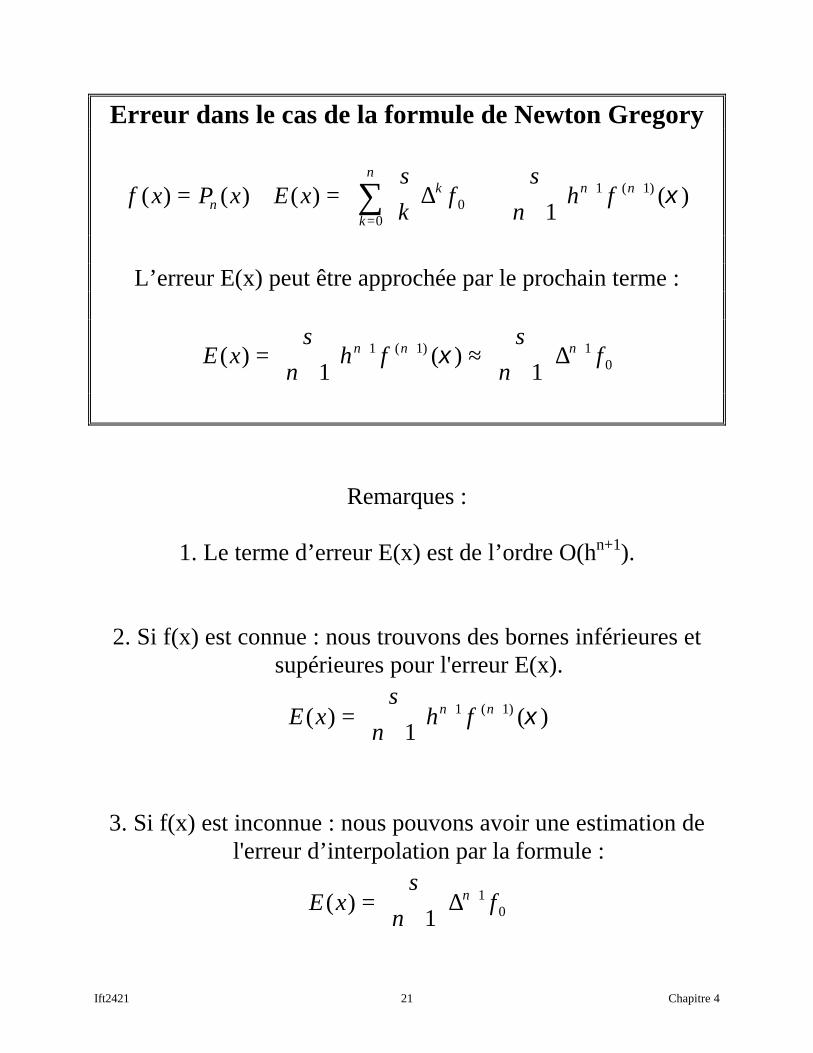
Erreur dans le cas de la formule de Newton Gregory

f x P x E xs

kf

s

nh fn

k

nk n n( ) ( ) ( ) ( )( )= + =

++

=

+ +∑0

01 1

1∆ ξ

L’erreur E(x) peut être approchée par le prochain terme :

E xs

nh f

s

nfn n n( ) ( )( )=

+

≈

+

+ + +

1 11 1 1

0ξ ∆

Remarques :

1. Le terme d’erreur E(x) est de l’ordre O(hn+1).

2. Si f(x) est connue : nous trouvons des bornes inférieures etsupérieures pour l'erreur E(x).

E x

s

nh fn n( ) ( )( )=

+

+ +

11 1 ξ

3. Si f(x) est inconnue : nous pouvons avoir une estimation del'erreur d’interpolation par la formule :

E xs

nfn( ) =

+

+

11

0∆

Ift2421 22 Chapitre 4

Exemple :

L’approximation de l’erreur sur Sin(0.8) avec le polynômequadratique avec x0 = 0.1.

x f(x)=∆0f ∆f ∆2f ∆3f ∆4f0.1 0.09983

0.379600.5 0.47943 -0.07570

0.30390 -0.047970.9 0.78333 -0.12367 0.01951

0.18023 -0.028461.3 0.96356 -0.15213

0.028101.7 0.99166

1. Nous ne connaissons pas la fonction f(x)Une approximation de l’erreur est donnée par :

E xs

fs s s

23

03

1 2

60 04797( )

( )( )( . )=

=

− −−∆

s = 2.5 0.8 -0.25 = 1.75

E2(0.8) = 0.002623

Remarque :Sin(0.8) - P2(0.8) = 0.00290422

Ift2421 23 Chapitre 4

2. Nous connaissons la fonction f(x) = Sin(x)L’erreur est donnée par :

E xs

h f23 3

3( ) ( )=

ξ avec 0.1 ≤ ξ ≤ 0.9

f3(x) = - Cos(x)

Es

h Cos2308

3( . ) ( )= −

ξ

0 62161 0 9 01 0 995004. ( . ) ( ) ( . ) .= ≤ ≤ =Cos Cos Cosξ

0 4 0 62161 0 4 0 9950043 3 3. . ( ) . .∗ ≤ ≤ ∗h Cos ξ

− ∗ ≥ − ≥ − ∗0 4 0 62161 0 4 0 9950043 3 3. . ( ) . .h Cos ξ

or x = 0.8 donc s = ( 0.8 - 0.1) / 0.4

ss s s

31

61 2

1

6

7

4

3

4

1

4

7

128

= − − = −

= −( )( )

7

1280 4 0 62161

37

1280 4 0 9950043 3 3. . ( ) . .∗ ≤ −

≤ ∗

sh Cos ξ

0 00217564 08 0 003482512. ( . ) .≤ ≤E

Ift2421 24 Chapitre 4

Avantages de la formules de Newton Gregory

1. Passage facile d’un polynôme de degré n à n+1.

P x P xs

nfn n

n+

+= ++

1

101

( ) ( ) ∆

2. La multiplication imbriquée minimise le nombre desopérations.

P x s s s

s s

2 0 09983 0 379600 07570

21

0 09983 0 379600 07570

21

( ) . ..

!( )

. ..

( )

= + +−

−

= + − −

3. Approximation simple de l’erreur commise.

Inconvénients

Intervalles égaux et points ordonnés

Ift2421 25 Chapitre 4

Différences diviséesDéfinitions :

Soit (xi , yi) i = 0, 1, ... , navec des intervalles irréguliers :

Les premières différences divisées sont :

[ ]∆ x xy y

x xou i j n i ji j

j i

j i

, , ,=−

−≤ ≤ ≠0

Les différences divisées du deuxième ordre sont :

[ ] [ ] [ ]∆

∆ ∆2 x x x

x x x x

x xi j k

j k i j

k i

, ,, ,

=−

−

Récursivement, les différences divisées du nième ordre sont

[ ] [ ] [ ]∆

∆ ∆n

n

nn

nn

n

x x xx x x x x x

x x0 1

11 2

10 1 1

0

, , ,, , , , , ,

ΚΚ Κ

=−

−

− −−

Nous avons donc une table des différences divisées.Exemple :

x0 y0

∆[x0,x1]x1 y1 ∆2[x0,x1,x2]

∆[x1,x2] ∆3[x0,x1,x2,x3]x2 y2 ∆2[x1,x2,x3]

∆[x2,x3]x3 y3

Ift2421 26 Chapitre 4

Formule de Newton pour les différences divisées

(cas où les abscisses sont quelconques)

Soit (xi,yi) i = 0, ... ,nAlors

[ ][ ]

P x f x x x x

x x x x x x x

n

nn n

( ) , ( )

, , , ( ) ( )

= + − +

+ − − −

0 0 1 0

0 1 0 1

∆

∆

Κ

Κ Κ

vérifie les n+1 conditions de collocations.

Ift2421 27 Chapitre 4

Exemple :Calculons le Polynôme de degré 3 passant par :

x0=0 y0=10

x1=1 y1=1 1/21 -1/12

x2=2 y2=2 1/63/2

x3=4 y3=5

P x a a x x a x x x x a x x x x x x3 0 1 0 2 0 1 3 0 1 2( ) ( ) ( ) ( ) ( ) ( )( )= + − + − − + − − −

P x x x x x x3 1 01

20 1

1

120 1 2( ) ( ) ( ) ( ) ( )( )= + + − − − − − −

P x x x x33 21

129 8 12( ) ( )= − + − +

1 2 3 4 5

1

2

3

4

5

6

P3(x)

X0X1

X2

X3

Ift2421 28 Chapitre 4

Calculons le Polynôme de degré 4 passant par les 4 pointsprécédents et ( x4 = 3, y4 = 5 ) :

P x a a x x a x x x x a x x x x x x

a x x x x x x x x4 0 1 0 2 0 1 3 0 1 2

4 0 1 2 3

( ) ( ) ( ) ( ) ( ) ( )( )

( ) ( )( )( )

= + − + − − + − − −+ − − − −

P x P x a x x x x x x x x4 3 4 0 1 2 3( ) ( ) ( ) ( )( )( )= + − − − −

donc

P x P x x x x x4 3

1

41 2 4( ) ( ) ( )( )( )= − − − −

P x x x x x44 3 21

4

5

3

11

4

4

31( ) = − + − + +

1 2 3 4 5

1

2

3

4

5

6

P44(x)

P3(x)

X0X1

X2

X3

X4

Ift2421 29 Chapitre 4

Instabilité des polynômes d’interpolation d’ordre élevé

Considérons la fonction définie par :

f(x) = 0 -1.2 ≤ x ≤ -0.2f(x) = 1 - | 5 x | -0.2 ≤ x ≤ 0.2f(x) = 0 0.2 ≤ x ≤ 1.0

-1 -0.5 0.5 1

-0.5

0.5

1

1.5

Ift2421 30 Chapitre 4

-1 -0.5 0.5 1

-0.5

0.5

1

1.5

P2(x)

-1 -0.5 0.5 1

-1

-0.5

0.5

1

1.5

P4(x)

Ift2421 31 Chapitre 4

-1 -0.5 0.5 1

-1

-0.5

0.5

1

1.5

P6(x)

-1 -0.5 0.5 1

-6

-5

-4

-3

-2

-1

1

P8(x)

Ift2421 32 Chapitre 4

Conclusion sur les polynôme de collocation

1. Degré assez grand mais pas trop.

2. Intervalle centré autour du point d’interpolation.

3. Il vaut mieux utiliser des polynômes de collocation de degrémoins grand sur différents sous intervalles.

Exemple :

f(x) estinterpolée par 3polynômes de

degré 2.-1 -0.5 0.5 1

-1

-0.5

0.5

1

1.5

Ift2421 33 Chapitre 4

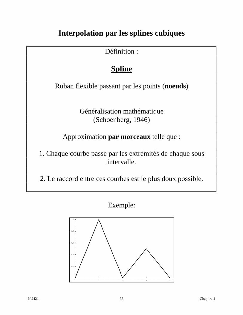
Interpolation par les splines cubiques

Définition :

Spline

Ruban flexible passant par les points (noeuds)

Généralisation mathématique(Schoenberg, 1946)

Approximation par morceaux telle que :

1. Chaque courbe passe par les extrémités de chaque sousintervalle.

2. Le raccord entre ces courbes est le plus doux possible.

Exemple:

1 2 3 4

0.2

0.4

0.6

0.8

1

Ift2421 34 Chapitre 4

Spline cubique

permet un raccord 2 fois différentiable :

Continuité de f, f’ et f’’.

Exemple:

1 2 3 4

0.2

0.4

0.6

0.8

1

Ift2421 35 Chapitre 4

Interpolation par les splines cubiques

Q x a x x b x x c x x d1 1 13

1 12

1 1 1( ) ( ) ( ) ( )= − + − + − +Q x a x x b x x c x x d2 2 2

32 2

22 2 2( ) ( ) ( ) ( )= − + − + − +

...Q x a x x b x x c x x di i i i i i i i( ) ( ) ( ) ( )= − + − + − +3 2

...Q x a x x b x x c x x dn n n n n n n n− − − − − − − −= − + − + − +1 1 1

31 1

21 1 1( ) ( ) ( ) ( )

Trouver ai, bi, ci, di pour i = 1,2, ... , n-1.

Ift2421 36 Chapitre 4

Condition 1 : Continuité des fonctions.y Q x1 1 1= ( )

y Q x Q x2 1 2 2 2= =( ) ( )...

y Q x Q xi i i i i= =−1( ) ( )...

y Q x Q xn n n n n− − − − −= =1 2 1 1 1( ) ( )y Q xn n n= −1( )

Condition 2 : Continuité des dérivées premières.′Q x1 1( )

′ = ′Q x Q x1 2 2 2( ) ( )...

′ = ′−Q x Q xi i i i1( ) ( )...

′ = ′− − − −Q x Q xn n n n2 1 1 1( ) ( )′−Q xn n1( )

Condition 3 : Continuité des dérivées secondes.′′ =Q x S1 1 1( )

′′ = ′′ =Q x Q x S1 2 2 2 2( ) ( )...

′′ = ′′ =−Q x Q x Si i i i i1( ) ( )...

′′ = ′′ =− − − − −Q x Q x Sn n n n n2 1 1 1 1( ) ( )′′ =−Q x Sn n n1( )

Ift2421 37 Chapitre 4

Condition 3 : Continuité des dérivées secondes.

a. i =1S Q x1 1 1= ′′( )

Q x a x x b x x c x x d1 1 13

1 12

1 1 1( ) ( ) ( ) ( )= − + − + − +′′ = − +Q x a x x b1 1 1 16 2( ) ( )

∴ S b1 12=

∴bS

11

2= pour i =1 (1)

b. i = 2, ... , n-1

S Q x Q xi i i i i= ′′ = ′′−1( ) ( )

Q x a x x b x x c x x di i i i i i i i( ) ( ) ( ) ( )= − + − + − +3 2

′′ = − +Q x a x x bi i i i( ) ( )6 2

∴ S Q x bi i i= ′′ =( ) 2

∴bS

ii=

2 pour i =2, ... , n-1 (2)

En combinant (1) et (2), nous obtenons :

∴bS

ii=

2 pour i =1, ... , n-1 (3)

Si on trouve S1, S2, ... , Sn-1, nous aurons b1, b2, ... , bn-1

Ift2421 38 Chapitre 4

Q x a x x b x x c x x di i i i i i i i− − − − − − − −= − + − + − +1 1 13

1 12

1 1 1( ) ( ) ( ) ( )′′ = − +− − − −Q x a x x bi i i i1 1 1 16 2( ) ( )

∴ S Q x Q xi i i i i= ′′ = ′′−1( ) ( )S a h bi i i i= +− − −6 21 1 1 or 2 1 1b Si i− −=

aS S

hii i

i−

−

−

=−

11

16 pour i =2, ... , n-1 (4)

∴ S S S a a an n1 2 1 1 2 2, , , , , ,Κ Κ− −⇒

c. i = nQ x a x x b x x c x x dn n n n n n n n− − − − − − − −= − + − + − +1 1 1

31 1

21 1 1( ) ( ) ( ) ( )

′′ = − +− − − −Q x a x x bn n n n1 1 1 16 2( ) ( )S a h b a h Sn n n n n n n= + = +− − − − − −6 2 61 1 1 1 1 1

∴ aS S

hnn n

n−

−

−

=−

11

16 pour i =n (5)

En combinant (4) et (5), nous obtenons :

aS S

hii i

i−

−

−

=−

11

16 pour i =2, ... , n-1, n (6)

ou alors

aS S

hii i

i

=−+1

6 pour i =1, 2, ... , n-1 (7)

∴ S S S a a an n1 2 1 2 1, , , , , ,Κ Κ⇒ −

Ift2421 39 Chapitre 4

Condition 1 : Continuité des fonctions.a. i =1

y Q x1 1 1= ( )

Q x a x x b x x c x x d1 1 13

1 12

1 1 1( ) ( ) ( ) ( )= − + − + − +

∴ d y1 1= pour i =1 (8)

b. i = 2, ... , n-1

y Q x Q xi i i i i= =−1( ) ( )

Q x a x x b x x c x x di i i i i i i i( ) ( ) ( ) ( )= − + − + − +3 2

∴ d yi i= pour i =2, ... , n-1 (9)

En combinant (8) et (9), nous obtenons :∴ d yi i= pour i =1, 2, ... , n-1 (10)

∴ y y y d d dn n1 2 1 1 2 1, , , , , ,Κ Κ− −⇒

de même:Q x a x x b x x c x x di i i i i i i i− − − − − − − −= − + − + − +1 1 1

31 1

21 1 1( ) ( ) ( ) ( )

∴ y a h b h c h di i i i i i i i= + + +− − − − − − −1 13

1 12

1 1 1

pour i =2, ... , n-1 (11)

Ift2421 40 Chapitre 4

c. i = ny Q xn n n= −1( )

Q x a x x b x x c x x dn n n n n n n n− − − − − − − −= − + − + − +1 1 13

1 12

1 1 1( ) ( ) ( ) ( )

∴ y a h b h c h dn n n n n n n n= + + +− − − − − − −1 13

1 12

1 1 1 (12)

En combinant (11) et (12), nous obtenons :

∴ y a h b h c h di i i i i i i i= + + +− − − − − − −1 13

1 12

1 1 1 pour i =2, ... , n (13)

ou bien

∴ y a h b h c h di i i i i i i i+ = + + +13 2

pour i =1, ... , n-1 (14)

dans (14) substituons ai, bi di par (3), (7), (10) et isolons Ci:

cy y

h

h S h Si

i i

i

i i i i=−

−++ +1 12

6 pour i =1, ... , n-1 (15)

∴ S S S c c cn n1 2 1 2 1, , , , , ,Κ Κ⇒ −

Ift2421 41 Chapitre 4

Condition 2 : Continuité des dérivées premières.Il ne reste donc qu'à trouver S1, S2, ... , Sn

a. i =1′ = ′Q x y notation1 1 1( ) ( )

Q x a x x b x x c x x d1 1 13

1 12

1 1 1( ) ( ) ( ) ( )= − + − + − +

′ = − + − +Q x a x x b x x c1 1 12

1 11

13 2( ) ( ) ( )

∴ ′ =y c1 1 pour i =1 (16)

b. i = 2, ... , n-1

′ = ′ = ′−y Q x Q xi i i i i1( ) ( )

′ = − + − +Q x a x x b x x ci i i i i i( ) ( ) ( )3 22 1

∴ ′=y ci i pour i = 2, ... , n-1 (17)

En combinant (16) et (17), nous obtenons :

∴ ′=y ci i pour i = 1, ... , n-1 (18)

∴ S S S c c c y y yn n n1 2 1 2 1 1 2 1, , , , , , , , ,Κ Κ Κ⇒ ⇒ ′ ′ ′− −

de même: ′ = − + − +− − − − − −Q x a x x b x x ci i i i i i1 1 12

1 1 13 2( ) ( ) ( )

∴ ′ = + +− − − − −y x a h b h ci i i i i i( ) 3 21 12

1 12

1 pour i = 2, ... , n-1 (19)

Ift2421 42 Chapitre 4

c. i = n

′ = ′−y Q xn n n1( )

Q x a x x b x x c x x dn n n n n n n n− − − − − − − −= − + − + − +1 1 13

1 12

1 1 1( ) ( ) ( ) ( )

′ = − + − +− − − − − −Q x a x x b x x cn n n n n n1 1 12

1 1 13 2( ) ( ) ( )

′ = + +− − − − − −Q x a h b h cn n n n n n1 1 12

1 1 13 2( ) pour i = n (20)

En combinant (19) et (20), nous obtenons :

′ = + +− − − − −y x a h b h ci i i i i n( ) 3 21 12

1 1 1 pour i = 2, ... , n (21)

En égalant (18) et (21) pour le domaine commun i = 2, ... , n-1,nous obtenons:

c a h b h ci i i i i i= + +− − − − −3 21 12

1 1 1 pour i = 2, ... , n-1 (22)

Ift2421 43 Chapitre 4

Dans (22), utilisons les formules (3), (7) et (15):

∴bS

ii=

2 pour i =1, ... , n-1 (3)

aS S

hii i

i

=−+1

6 pour i =1, 2, ... , n-1 (7)

cy y

h

h S h Si

i i

i

i i i i=−

−++ +1 12

6 pour i =1, ... , n-1 (15)

pour i = 2, ... , n-1, nous obtenons:

y y

h

h S h S S S

hh

Sh

y yh

h S h S

i i

i

i i i i i i

ii

ii

i i

i

i i i i

+ + −

−−

−−

−

−

− − −

−−

+=

−

+

+−

−+

1 1 1

11

2

11

1

1

1 1 1

2

63

6

22

2

6

( )

( )

∴ h S h h S h Sy y

h

y y

hi i i i i i ii i

i

i i

i− − − +

+ −

−

+ + + =−

−−

1 1 1 1

1 1

1

2 2 6( )

Pour i = 2, ... , n-1 donc (n-2) équations à n inconnues S1, ... , Sn

Ift2421 44 Chapitre 4

Nous avons un système de (n-2) équationsà n inconnues S1, ... , Sn à résoudre.

i h S h h S h Sy y

h

y y

h

i h S h h S h Sy y

h

y y

h

i h S h h S h Sy y

h

y y

h

i n h Sn n

= + + + =−

−−

= + + + =−

−−

= + + + =−

−−

= − +− −

2 2 6

3 2 6

4 2 6

1 2

1 1 1 2 2 2 33 2

2

2 1

1

2 2 2 3 3 3 44 3

3

3 2

2

3 3 3 4 4 4 55 4

4

4 3

3

2 2

( )

( )

( )

( )h h S h Sy y

h

y y

hn n n n nn n

n

n n

n− − − −

−

−

− −

−

+ + =−

−−

2 1 1 1

1

1

1 2

2

6

Nous réduisons ce système à (n-2) inconnues en imposant des valeurs(Conditions frontières) pour S1 et Sn aux extrémités de l'intervalle:

x x

x x x

x x x

x x x

x x x

x x

S

S

S

S

S

z

z

z

z

zn

n

n

n

0

0

2

3

4

2

1

2

3

4

2

1

Ο Ο Ο

Ο Ο Ο

Μ

Μ

Μ

Μ

Μ

Μ

⋅

=

−

−

−

−

⇒ ⇒ ⇒S S S a b c d Q xn i i i i i1 2, , , , , , ( )Κ

Ift2421 45 Chapitre 4

Les coefficients de chaque polynôme de degré 3

Q x a x x b x x c x x d1 1 13

1 12

1 1 1( ) ( ) ( ) ( )= − + − + − +Q x a x x b x x c x x d2 2 2

32 2

22 2 2( ) ( ) ( ) ( )= − + − + − +

...Q x a x x b x x c x x di i i i i i i i( ) ( ) ( ) ( )= − + − + − +3 2

...Q x a x x b x x c x x dn n n n n n n n− − − − − − − −= − + − + − +1 1 1

31 1

21 1 1( ) ( ) ( ) ( )

sont donnés par :

( )

( )

aS S

h

bS

cy y

h

S S h

d y

ii i

i

ii

ii i

i

i i i

i i

=−

=

=−

−+

=

+

+ +

1

1 1

6

2

2

6

Ift2421 46 Chapitre 4

Splines cubiques : Conditions frontières

1. Extrémités libres (free boundary conditions) Type 1

Dans les splines dites Naturelles (natural spline), nous ajoutonsles 2 équations :

S1 = 0Sn = 0

La spline a un comportement parabolique linéaire aux bouts.(près de extrémités)

La première équation devient :

2 61 2 2 2 33 2

2

2 1

1

( )h h S h Sy y

h

y y

h+ + =

−−

−

La dernière équation devient :

h S h h Sy y

h

y y

hn n n n nn n

n

n n

n− − − − −

−

−

− −

−

+ + =−

−−

2 2 2 1 1

1

1

1 2

2

2 6( )

Ift2421 47 Chapitre 4

Exemple :

Faire passer une spline cubique naturelle par les points suivants :

i 1 2 3 4xi 1 2 3 4

f(xi) 4 -2 3 1

Spline naturelle : S1 = 0 et S4 = 0

2

2

6

6

1 2 2

2 2 3

2

3

3 2

2

2 1

1

4 3

3

3 2

2

( )

( )

h h h

h h h

S

S

y yh

y yh

y yh

y yh

++

⋅

=

−−

−

−−

−

[ ][ ]

4 1

1 4

6 3 2 2 4

6 1 3 3 22

3

⋅

=

+ − − −− − +

S

S( ) ( )

( ) ( )

4 1

1 4

66

422

3

⋅

=

−

S

S

Nous avons donc la solution :

S1 = 0, S2 = 20.4, S3 = -15.6 et S4 = 0

Ift2421 48 Chapitre 4

( )

( )

aS S

hb

S

cy y

h

S S h

d y

12 1

11

1

12 1

1

1 2 1

1 1

6 2

2

6

=−

=

=−

−+

=

, ,

,

a b c d1 1 1 134 0 9 4 4= = = − =. , , . ,

Q x x x133 4 1 9 4 1

4

( ) . ( ) . ( )= − − −+

1 2 3 4

-2

0

2

4

6

Q1(x)

( )

( )

aS S

hb

S

cy y

h

S S h

d y

23 2

22

2

23 2

2

2 3 2

2 2

6 2

2

6

=−

=

=−

−+

=

, ,

,

a b c

d2 2 2

2

6 10 2 0 8

2

= − = == −

, . , . ,

Q x x x

x2

3 26 2 10 2 2

0 8 2 2

( ) ( ) . ( )

. ( )

= − − + −+ − −

1 2 3 4

-2

0

2

4

6

Q2(x)

Ift2421 49 Chapitre 4

( )

( )

aS S

hb

S

cy y

h

S S h

d y

34 3

33

3

34 3

3

3 4 3

3 3

6 2

2

6

=−

=

=−

−+

=

, ,

,

a b c d3 3 3 32 6 7 8 32 3= = − = =. , . , . ,

Q x x x

x3

3 22 6 3 7 8 3

3 2 3 3

( ) . ( ) . ( )

. ( )

= − − −+ − +

1 2 3 4

-2

0

2

4

6

Q3(x)

1 2 3 4

-2

0

2

4

6

Q1(x)

Q2(x)Q3(x)

Ift2421 50 Chapitre 4

2. nous ajoutons les 2 conditions : Type 2

S1 = S2

Sn = Sn-1

La spline a un comportement parabolique aux bouts.(près des extrémités)

La première équation devient :

( )3 2 61 2 2 2 33 2

2

2 1

1

h h S h Sy y

h

y y

h+ + =

−−

−

La dernière équation devient :

h S h h Sy y

h

y y

hn n n n nn n

n

n n

n− − − − −

−

−

− −

−

+ + =−

−−

2 2 2 1 1

1

1

1 2

2

2 3 6( )

Exemple (suite)

Utilisons des conditions frontières de type 2.

S1 = S2 = 15.5S3 = S4 = -11.5

Ift2421 51 Chapitre 4

3. nous ajoutons les 2 conditions : Type 3

S1 = Extrapolation linéaire de S2 et S3

Sn = Extrapolation linéaire de Sn-2 et Sn-1

S S

h

S S

h3 2

2

2 1

1

−=

− S S

h

S S

hn n

n

n n

n

− −

−

−

−

−=

−2 1

2

1

1

S Sh h

h

h

hS1 2

1 2

2

1

23=

+

− S

h

hS

h h

hSn

n

nn

n n

nn= − +

+

−

−−

− −

−−

1

22

2 1

21

La première équation devient :( )( ) ( )

Sh h h h

hS

h h

hy y

hy y

h2

1 2 1 2

23

22

12

2

3 2

2

2 1

1

26

+ +

+

−=

−−

−

La dernière équation devient :( ) ( )( )

Sh h

hS

h h h h

hy y

hy y

hnn n

nn

n n n n

n

n n

n

n n

n−

− −

−−

− − − −

−

−

−

− −

−

−+

+ +

+ =

−−

−

2

22

12

21

1 2 1 2

2

1

1

1 2

2

26

Exemple (suite) : S1 = 29, S2 = 11, S3 =-7, S4 = -25

Ift2421 52 Chapitre 4

4. nous imposons des valeurs aux pentes des extrémités Type 4

′ = ′Q x y1 1 1( ) Imposée′ = ′−Q x yn n n1( ) Imposée

Q x a x x b x x c x x d1 1 13

1 12

1 1 1( ) ( ) ( ) ( )= − + − + − +

′ = − + − +Q x a x x b x x c1 1 12

1 1 13 2( ) ( ) ( )

′ = = ′Q x c y1 1 1 1( )

( )y y

h

S S hy2 1

1

1 2 1

1

2

6

−−

+= ′

hS

hS

y y

hy1

11

22 1

113 6

+ =−

− ′ (a)

Ift2421 53 Chapitre 4

De même

Q x a x x b x x c x x dn n n n n n n n− − − − − − − −= − + − + − +1 1 13

1 12

1 1 1( ) ( ) ( ) ( )

′ = − + − +− − − − − −Q x a x x b x x cn n n n n n1 1 12

1 1 13 2( ) ( ) ( )

′ = + + = ′− − − − − −Q x a h b h c yn n n n n n n1 1 12

1 1 13 2( )

36

22

2

61

11

2 11

1

1

1 1 1S S

hh

Sh

y y

h

h S h Syn n

nn

nn

n n

n

n n n nn

−+ +

−−

+

= ′−

−−

−−

−

−

− − −

hS

hS y

y y

hn

nn

n nn n

n

−−

− −

−

+ = ′ −−1

11 1

16 3 (b)

Nous devons maintenant ajouter ces 2 équations aux n-2équations que nous avons déjà, et résoudre le système de n

équations à n inconnues.

Ift2421 54 Chapitre 4

Exemple :

Faire passer des splines cubiques par les points suivants :Avec des conditions frontières de types 1, 2 et 3.

i 1 2 3 4 5 6xi 1 2 3 4 5 6

f(xi) 4 -2 3 1 4 0

La résolution du système nous donne:

=

38.6

11

16.6

13.4

7

27.4

=Stype 1

0

21.474

19.895

16.105

14.526

0

=

16.893

16.893

18.464

14.964

11.393

11.393

Stype 2Stype 3

0 1 2 3 4 5 6 7 85

0

5

10

yi

interp( ),,,dl x y x2

interp( ),,,dp x y x2

interp( ),,,dc x y x2

,xi

x2

Ift2421 55 Chapitre 4

Interpolation par les splines cubiquesAlgorithme de résolution de système tridiagonal

a a

a a a

a a a

a a a

a a a

a a a

a a

S

S

S

S

S

S

S

1 2 1 3

2 1 2 2 2 3

3 1 3 2 3 3

4 1 4 2 4 3

5 1 5 2 5 3

6 1 6 2 6 3

7 1 7 2

1

2

3

4

5

6

7

0 0 0 0 0

0 0 0 0

0 0 0 0

0 0 0 0

0 0 0 0

0 0 0 0

0 0 0 0 0

, ,

, , ,

, , ,

, , ,

, , ,

, , ,

, ,

=

a

a

a

a

a

a

a

1 4

2 4

3 4

4 4

5 4

6 4

7 4

,

,

,

,

,

,

,

Une résolution par élimination de Gauss est équivalente à :

1. Factorisation :

a aa

aa a pour i n

a aa

aa a a

i ii

ii i

i ii

ii i i

, ,,

,, ,

, ,,

,, , ,

, ,2 21

1 21 3 1

4 41

1 21 4 3 3

0 2= − = =

= − =

−−

−−

Κ

2. Substitution arrière :

aa

apour i n

aa a a

a

nn

n

ii i i

i

,

,

,

,

, , ,

,

, ,

*

4

4

2

4

4 3 1 4

2

1 1= = −

=− +

Κ

Ift2421 56 Chapitre 4

Les lignes courbes : Courbes de Bézier

Inventées dans le but de mieux contrôler la conception (CAO)d’automobile chez la compagnie Renault par Pierre Bézier.

La notion de points de contrôle apparaît dans le but demanipuler la courbe plus facilement.

Cependant, la modification d'un seul point de contrôle entraîneune modification de la courbe entière: on parle alors de contrôle

global.

On se libère de cette contrainte en définissant une courbe deBézier par morceau.

On peut définir une portion de courbe de Bézier à partir de n+1points à l'aide de polynômes particuliers qui jouent le rôle de

facteurs de pondération entre les points.

Le polynôme de Bézier de degré n est donné par :

P un

iu u p avec

n

in

i n in i i

ii

n

( ) ( )!

!( )!=

−

=

−−

=∑ 1

0

Représentation paramétrique :

p ux u

y uavec u( )

( )

( )=

≤ ≤0 1

Ift2421 57 Chapitre 4

avec px

yi

i

i

=

0 ≤ i ≤ n (n+1 points)

Ces fonctions de pondération sont les polynômes de Bernstein.

BEZ un

iu ui n

n i i, ( ) ( )=

− −1

Le polynôme de Bézier de degré n est équivalent à :

x un

iu u xn i i

ii

n

( ) ( )=

− −

=∑ 1

0

y un

iu u yn i i

ii

n

( ) ( )=

− −

=∑ 1

0

Remarque :

BEZ uk

ku u uk k

k k k k, ( ) ( )=

− =−1

BEZ uk

u u ukk k

00 0

01 1, ( ) ( ) ( )=

− = −−

Ift2421 58 Chapitre 4

Courbes de Bézier cubiques :

Nous avons alors les polynômes de Bernstein suivants :

BEZ u0 331, ( )= −

BEZ u u u1 323 1, ( ) ( )= −

BEZ u u u2 323 1, ( ) ( )= −

BEZ u u3 33

, ( ) =

doncx u u x u u x u u x u x( ) ( ) ( ) ( )= − + − + − +1 3 1 3 13

02

12

23

3

y u u y u u y u u y u y( ) ( ) ( ) ( )= − + − + − +1 3 1 3 130

21

22

33

Ift2421 59 Chapitre 4

Propriétés des courbes de Bézier :

1. Une courbe de Bézier passe toujours par le premier et ledernier point.

p p( )0 0=p pn( )1 =

2. La courbe de Bézier est contenue dans l'enveloppe convexeformée par les points de contrôle.

L'enveloppe convexe d'un ensemble de points est le plus petitensemble convexe contenant tout ces points.

3. À u = 0, dxdu

x x= −3 1 0( ) et dydu

y y= −3 1 0( )

La pente de la courbe à u = 0 est dydx

y y

x x=

−−

( )

( )1 0

1 0.

C'est la pente de la droite passant par p0 et p1.

De la même façon, en u =1, la pente de la courbe de Bézier audernier point est la même que la pente de la droite joignant les 2

derniers points.

Ift2421 60 Chapitre 4

Ift2421 61 Chapitre 4

P2, P3 et P4 ne sont pas alignés.

P2, P3 et P4 sont alignés.

Ift2421 62 Chapitre 4

Ift2421 63 Chapitre 4

Représentation matricielle des courbes de Bézier cubiques :

P un

iu u p avec

n

in

i n in i i

ii

n

( ) ( )!

!( )!=

−

=

−−

=∑ 1

0

peut être écrit pour une courbe de Bézier cubique:

[ ]P u u u u

p

p

p

p

( ) , , ,=

− −−

−

3 2

0

1

2

3

1

1 3 3 1

3 6 3 0

3 3 0 0

1 0 0 0

P u u M pTBez( ) =

Ift2421 64 Chapitre 4

Exemple d'utilisation des courbes de Bézier :

Courbe Fermée:

Passage plus proche d'un point de contrôle:

Ift2421 65 Chapitre 4

Les Surfaces courbes de Bézier: 3D

Pour étendre les calculs précédents à des surfaces, il s'agitd'ajouter un paramètre v et la surface est donnée par:

P u v p BEZ v BEZ uj k j m k nk

n

j

m

( , ) ( ) ( ), , ,===

∑∑00

Pour des surfaces de Béziers cubiques, nous allons avoir besoinde 16 points (4x4)

en notation matricielle, nous avons :

[ ] [ ]x u v u u u M X M v v vBez BezT T

( , ) = 3 2 3 21 1

[ ] [ ]y u v u u u M Y M v v vBez BezT T

( , ) = 3 2 3 21 1

[ ] [ ]z u v u u u M Z M v v vBez BezT T

( , ) = 3 2 3 21 1

avec X

x x x x

x x x x

x x x x

x x x x

=

0 0 0 1 0 2 0 3

1 0 1 1 1 2 1 3

2 0 2 1 2 2 2 3

3 0 3 1 3 2 3 3

, , , ,

, , , ,

, , , ,

, , , ,

Ift2421 66 Chapitre 4

Les lignes courbes: Courbe B-Spline cubique

B-Spline cubique:

Inventée aussi dans le but de mieux contrôler le design.(DAO etCAO).

La notion de points de contrôle existe aussi dans le but demanipuler la courbe plus facilement mais contrairement auxcourbes de Bézier, l'effet de la manipulation d’un point de

contrôle demeure locale.

On peut définir une portion de courbe de B-Spline cubique àpartir de 4 points avec l'aide de polynômes particulier qui jouent

le rôle de fonctions de "mélange" entre les points.

Contrairement aux courbes de Bézier cependant, les ler et 4e

points n’appartiennent pas nécessairement par la courbe ainsi les4 points agissent comme des points de contrôle.

Ift2421 67 Chapitre 4

Comme pour les splines cubiques, les mêmes contraintes decontinuité sont utilisées pour joindre les segments de B-Splines.

On prend des groupes de 4 points se chevauchants :

Cependant si on désire terminer la courbe aux points extrémitésP0 et Pn, il suffit de générer 4 nouveaux points

i.e. P-1 = P-2 = P0 ainsi que Pn+1 = Pn+2 = Pn.

Ift2421 68 Chapitre 4

L’équation paramétrique d’une B-Spline cubique est :

pour n+1 points pi =(xi,yi) i = 0, ... ,n.La B-Spline cubique pour l’intervalle (pi,pi+1)

pour i = 1,2,..., n-1

B u b pi k i kk

( ) = +=−∑

1

2

avec

où les bi sont des fonctions de ‘mélange’.

bu

bu

u

bu u u

bu

u

− =−

= − +

= − + + +

= ≤ ≤

1

3

0

32

1

3 2

2

3

1

6

2

2

3

2 2 2

1

6

60 1

( )

,

Ift2421 69 Chapitre 4

Représentation matricielle des courbes de B-Splinescubiques :

B u b pi k i kk

( ) = +=−∑

1

2

peut être écrit pour une courbe B-Spline cubique:

[ ]B u u u u

p

p

p

p

i

i

i

i

i

( ) , , ,=

− −−

−

−

+

+

1

61

1 3 3 1

3 6 3 0

3 0 3 0

1 4 1 0

3 2 1

1

1

2

B uu M p

i

Tb( ) =

6

Ift2421 70 Chapitre 4

Passer par les extrémités dans les courbes B-Splinescubiques :

Démonstration :

Si nous désirons terminer la courbe aux points extrémités p0 etpn, il suffit de générer 4 nouveaux points:

p-2 = p-1 = p0 et pn+2 = pn+1 = pn

L’équation de la B-Spline est :

[ ]B u u u u

p

p

p

p

i

i

i

i

i

( ) , , ,=

− −−

−

−

+

+

1

61

1 3 3 1

3 6 3 0

3 0 3 0

1 4 1 0

3 2 1

1

1

2

Ift2421 71 Chapitre 4

Évaluons cette équation pour le nouveau premier segment c-à-dB-1 en posant p-2 = p-1 = p0 alors :

[ ]B u u u u

p

p

p

p

−

−

−=

− −−

−

13 2 1

2

1

0

1

1

61

1 3 3 1

3 6 3 0

3 0 3 0

1 4 1 0

( ) , , ,

[ ]B u u u u

p

p

p

p

− =

− −−

−

13 2 1

0

0

0

1

1

61

1 3 3 1

3 6 3 0

3 0 3 0

1 4 1 0

( ) , , ,

B u p p u p− = − +1 1 03

0

1

6( ) ( )

Pour u = 0, nous obtenons bien : B-1(0) = p0.

Note : un développement similaire peu être fait pour pn.

Ift2421 72 Chapitre 4

Ift2421 73 Chapitre 4

Joindre 2 courbes B-Spline:

p2 , p3 et p4 ne sont pas alignés

p2 , p3 et p4 sont alignés

Ift2421 74 Chapitre 4

Les Surfaces courbes B-Spline : 3D

Pour étendre les calculs précédents à des surfaces, il s'agitd'ajouter un paramètre v et la surface est donnée par:

[ ] [ ]x u v u u u M X M v v vb i j bT T

( , ) ,=1

361 13 2 3 2

[ ] [ ]y u v u u u M Y M v v vb i j bT T

( , ) ,=1

361 13 2 3 2

[ ] [ ]z u v u u u M Z M v v vb i j bT T

( , ) ,=1

361 13 2 3 2

avec X

x x x x

x x x x

x x x x

x x x x

i j

i j i j i j i j

i j i j i j i j

i j i j i j i j

i j i j i j i j

,

, , , ,

, , , ,

, , , ,

, , , ,

=

− − − − + − +

− + +

+ − + + + + +

+ − + + + + +

1 1 1 1 1 1 2

1 1 2

1 1 1 1 1 1 2

2 1 2 2 1 2 2

Pour des surfaces B-Splines cubiques, nous allons avoir besoinde 16 points (4x4)

Ift2421 75 Chapitre 4

Interpolation de surfaces par des surfacespolynomiales de collocation

But : interpoler un point en 3 dimensions.

Pour une fonction à 2 variables z = f(x,y)

x\y 0.2 0.3 0.4 0.51.0 0.640 1.003 1.359 1.7031.5 0.990 1.524 2.045 2.5492.0 1.568 2.384 3.177 3.943

z f x y e Sin y yx= = + −( , ) ( ) .01

Nous voulons interpoler la valeur de la fonction en f(1.6,0.33).

2 approches possibles :

1. Interpoler directement la fonction au point considéré.

2. Calculer l'équation de la surface de collocation et utiliserl’équation de cette surface pour interpoler la valeur de la

fonction au point d'intérêt.

Ift2421 76 Chapitre 4

1. Interpoler directement la fonction au point considéré.

0

1

2

3

x

0.1

0.2

0.30.4

0.5 y

0

1

2

3

4

z

0

1

2

3

x

0.1

0.2

0.30.4

0.5 y

1

2

3

4

5

6

7

8

9

10

11

12

Ensemble de points

Pour x constant,interpolation en y.

01 2 3x

0.10.20.30.40.5

y

0

1

2

3

4

z

0

1

2

3

4

z

1

2

3

4

A 5

6

7

8

B 9

10

11

12

C

Ift2421 77 Chapitre 4

Interpolation en x pour y = 1.6

0

1

2

3

x

0.1

0.2

0.30.4

0.5 y

0

1

2

3

4

z

0

1

2

3

x

0.1

0.2

0.30.4

0.5 y

1

2

3

4

A

5

6

7

8

B

9

10

11

12

C

A

B

C

X

0 1 2 3

x

0.10.20.30.40.5

y

0

1

2

3

4

z

0 1 2 3

x

0.10.20.30.40.5

y

1

2

3

4

A

5

6

7

8

B

9

10

11

12

C

A

B

C

X

Ift2421 78 Chapitre 4

Interpolation en yy z ∆∆z ∆∆2z ∆∆3z

0.2 0.6400.363

0.3 1.003 -0.007x = 0.1 0.356 -0.005

0.4 1.359 -0.0120.344

0.5 1.7030.2 0.990

0.5340.3 1.524 -0.013

x = 1.5 0.521 -0.0040.4 2.045 -0.017

0.5040.5 2.5490.2 1.568

0.8160.3 2.384 -0.023

x = 2.0 0.793 -0.0040.4 3.177 -0.027

0.7660.5 3.943

Étape 1 :x = 1.0

z P y zS

zS

zS

z= = +

+

+

3 0 0

20

301 2 3

( ) ∆ ∆ ∆

S=(y-y0)/h = (0.33-0.2)/0.1 = 1.3

P3(0.33) = 0.640+1.3*0.363+1.3*0.3*(-0.007)/2+1.3*0.3*(-0.7)(-0.005)/6

P3(0.33) = 1.1108

Ift2421 79 Chapitre 4

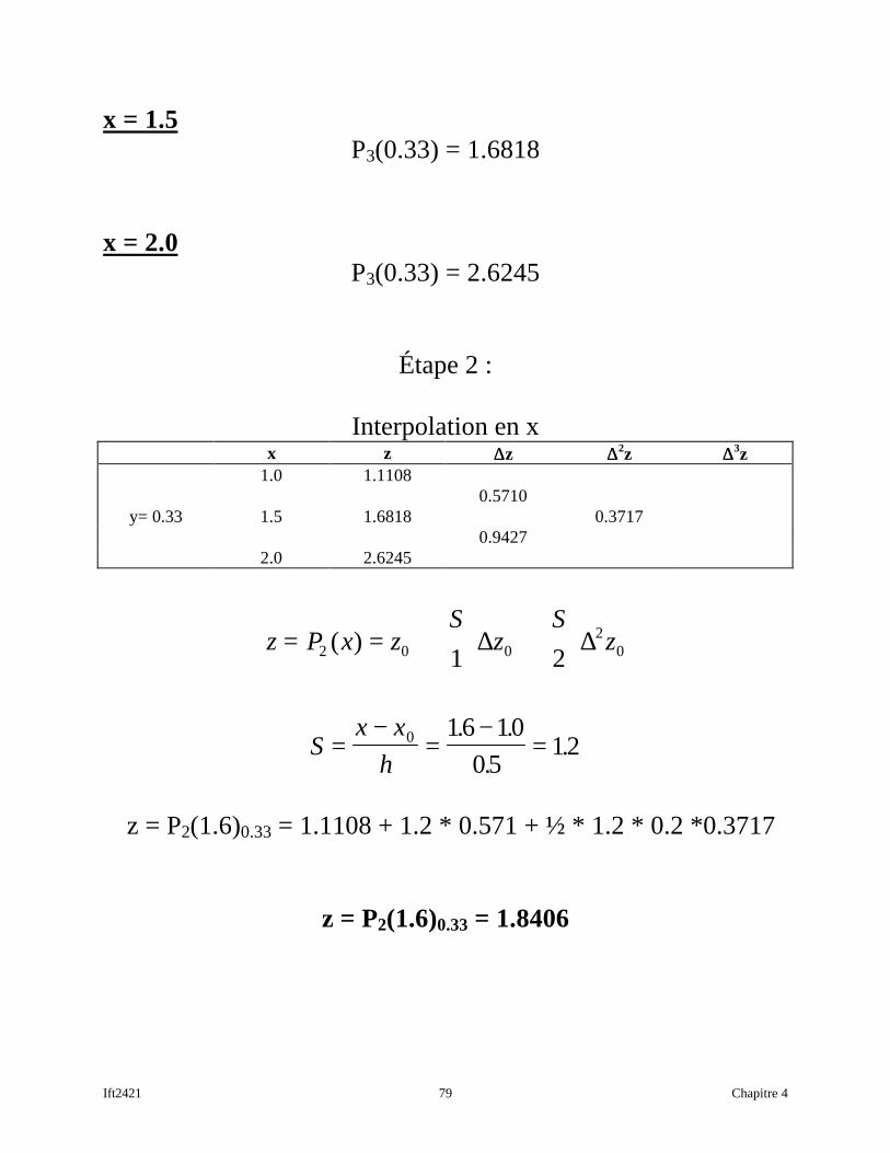
x = 1.5P3(0.33) = 1.6818

x = 2.0P3(0.33) = 2.6245

Étape 2 :

Interpolation en xx z ∆∆z ∆∆2z ∆∆3z

1.0 1.11080.5710

y= 0.33 1.5 1.6818 0.37170.9427

2.0 2.6245

z P x zS

zS

z= = +

+

2 0 0

201 2

( ) ∆ ∆

Sx x

h=

−=

−=0 16 10

0512

. .

..

z = P2(1.6)0.33 = 1.1108 + 1.2 * 0.571 + ½ * 1.2 * 0.2 *0.3717

z = P2(1.6)0.33 = 1.8406

Ift2421 80 Chapitre 4

2. Calculer l'équation de la surface de collocation et utiliserl’équation de cette surface.

L'équation de la surface de collocation est:

P2,3(x,y) = -0.065 - 0.018 x - 0.004 x2 + 3.28167 y - 2.02667 x y+ 2.33333 x2 y + 1.15 y2 - 0.65 x y2 - 0.1 x2 y2 - 1.66667 y3 +

1.16667 x y3 - 0.333333 x2 y3

0

1

2

3

x

0.1

0.2

0.30.4

0.5 y

0

1

2

3

4

z

0

1

2

3

x

0.1

0.2

0.30.4

0.5 y

1

2

3

4

5

6

7

8

9

10

11

12

P(0.33, 1.6) = 1.8406

Ift2421 81 Chapitre 4

Ift 2421

Chapitre 4

Interpolationpolynomiale :

Moindres carrés

Ift2421 82 Chapitre 4

Introduction

Ti (°C) Ri (ohms)20.5 76532.7 82651.0 87373.2 94295.7 1032

Lissage par moindres carrés(régression linéaire)

Quelle est la meilleuredroite ?

(observation ou théorie)

R = a T + b

Ift2421 83 Chapitre 4

Lissage par moindres carrés

But :

Trouver un polynôme de degré fable passant par beaucoup depoints.

Déterminer Pn(x) avec n ≤ m-1qui minimise l’écart quadratique

R e e e eN2 12

22

32 2= + + + +{ } { } { } { }Κ

Ift2421 84 Chapitre 4

Lissage par moindres carrés(régression linéaire)

Dans le cas de la droite, P1(x) = a x + b = y

Soit ei = Yi - yi

R eii

m

22

1

==∑

R Y y Y a x b R a bi ii

m

i ii

m

22

1

22

1

= − = − − == =∑ ∑( ) ( ) ( , )

Trouver a et b pour que R2 soit minimum.

RR

aet

R

a22 20 0min ⇒ = =

∂∂

∂∂

∂∂

∂∂

R

aY a x b

aY a x bi i i i

i

m2

1

2 0= − − − −

=

=∑ ( ) ( )

∂∂

∂∂

Rb

Y a x bb

Y a x bi i i ii

m2

1

2 0= − − − −

=

=∑ ( ) ( )

( )

( )

( )(

( )(

Y a x b x

Y a x b

i i ii

m

i ii

m

− − − =

− − − =

=

=

∑

∑

0

1 0

1

1

Équations Normales

a x b x x y

a x bm y

i i i i

i i

2∑ ∑ ∑∑ ∑

+ =

+ = ⇒ a, b : y=ax + b

Ift2421 85 Chapitre 4

Lissage par moindres carrés(régression linéaire)

Exemple :Ti (°C) Ri (ohms) Ti

2 Ti Ri

20.5 76532.7 82651.0 87373.2 94295.7 1032

Total : 273.1 4438 18607.27 254932.5

18607 27 2731

2731 5 0

254932 5

4438 0

. .

. .

.

.

=

a

b

P1(x) = a x + b = 3.395 x + 702.2

Ift2421 86 Chapitre 4

Remarque : les problèmes de ce type peuvent aussi être résoluspar la méthode des systèmes surdéterminés.

y ax b

y ax b

y ax b

x

x

x

a

b

y

y

y

A Ax A b

m m m m

T T

1 1

2 2

1

2

1

2

1

1

1

1

= += +

= +

⇔

=

⇒ =Μ Μ Μ

x x x

x

x

x

a

b

x x x

y

y

y

m

m

m

m

1 2

1

2 1 2

1

2

1 1 1

1

1

1

1 1 1

Κ

Μ

Κ

⋅

⋅

=

⋅

x x x x x x

x x x m

a

b

x y x y x y

y y ym m

m

m m

m

12

22 2

1 2

1 2

1 1 2 2

1 2

+ + + + + ++ + +

⋅

=

+ + ++ + +

Κ Κ

Κ

Κ

Κ

x x

x m

a

bx y

yi i

i

i i

i

2∑ ∑∑

∑∑

⋅

=

a x b x x y

a x bm y

i i i i

i i

2∑ ∑ ∑∑ ∑

+ =

+ =

Ift2421 87 Chapitre 4

Lissage par moindres carrés(régression non linéaire)

Polynôme

Dans d’un polynôme de degré arbitraire,

Pn(x) = a0 + a1 x + a2 x2 + ... + an x

n

Soit ei = Yi - Pn(xi)

( )( )R e Y P xii

m

i N ii

m

22

1

2

1

= = −= =∑ ∑

Minimum pour :

∂∂Ra

Y P x xj

i N i ij

i

m2

1

2 0= − − ==∑ ( ( ))( )

11 1 1

1

2

1

1

1

1

1

1

2

1

0

1

1

1

1

i

m

ii

m

iN

i

m

ii

m

ii

m

iN

i

m

iN

i

m

iN

i

m

iN

i

mN

ii

m

i ii

m

iN

ii

m

x x

x x x

x x x

a

a

a

x

x y

x y

= = =

= =

+

=

=

+

= =

=

=

=

∑ ∑ ∑

∑ ∑ ∑

∑ ∑ ∑

∑

∑

∑

⋅

=

Κ

Κ

Κ Κ Κ Κ

Κ

ΚΚ

Ift2421 88 Chapitre 4

Lissage par moindres carrés(régression non linéaire)Différent d’un polynôme

Autre formes :

1. y = a xb

2. y = a ebx

Nous obtenons des systèmes linéaires difficiles à résoudre.

Changement de variables :

z = ln(y)w = ln(x)

1. ln(y) = ln(a) + b ln(x)Modifications qui conduisent à la méthode linéaire :

z = A + b w

2. ln(y) = ln(a) + b xModifications qui conduisent à la méthode linéaire :

z = A + b x

Ift2421 89 Chapitre 4

Exemple : Régression en y = a ebx avec la table :

x 1.0 2.0 4.0y 2.0 7.2 500.1

2. ln(y) = ln(a) + b x

x 1.0 2.0 4.0ln(y) 0.693 1.974 6.215

Modifications qui conduisent à la méthode linéaire :z = A + b x

x z = ln(y) x2 x ln(y)1 0.693 1 0.6932 1.974 4 3.9484 6.215 16 24.859

x x

x m

b

Ax z

zi i

i

i i

i

2∑ ∑∑

∑∑

⋅

=

21 7

7 3

29 5

8882

⋅

=

b

A

.

.

b

A

b

a e

=

−

⇒

== =−

188

1427

188

0 241 427

.

.

.

..1 2 3 4

0

100

200

300

400

500

600

Ift2421 90 Chapitre 4

Autres méthodes de lissage

Moindres carrés : méthode populaire

D’autres méthodes de lissagebasées sur d’autres mesures pour l’erreur,

par exemple :

R ei m

i∞≤ ≤

=1

max

R eii

m

11

==∑

La méthode des moindres carrés est pratique pourprincipalement deux raisons :

1. L’écart quadratique est dérivable (pas de valeur absolue).

2. En accord avec le principe de vraisemblance maximale desstatistiques.