IEEE TRANSACTIONS ON EVOLUTIONARY COMPUTATION, VOL. X, NO. Y, MONTH YEAR 1 Frequency Fitness Assignment Thomas Weise, Member, IEEE, Mingxu Wan, Member, IEEE, Pu Wang, Member, IEEE, Ke Tang, Member, IEEE, Alexandre Devert, and Xin Yao, Fellow, IEEE Abstract—Metaheuristic optimization procedures such as Evo- lutionary Algorithms are usually driven by an objective function which rates the quality of a candidate solution. However, it is not clear in practice whether an objective function adequately rewards intermediate solutions on the path to the global optimum and it may exhibit deceptiveness, epistasis, neutrality, ruggedness, and a lack of causality. In this paper, we introduce the Frequency Fitness H, subject to minimization, that rates how often solutions with the same objective value have been discovered so far. The ideas behind this method are that good solutions are hard to find and that if an algorithm gets stuck at a local optimum, the frequency of the objective values of the surrounding solutions will increase over time, which will eventually allow it to leave that region again. We substitute a Frequency Fitness Assignment process (FFA) for the objective function into several different optimization algorithms. We conduct a comprehensive set of experiments: the synthesis of algorithms with Genetic Program- ming (GP), the solution of MAX-3SAT problems with Genetic Algorithms, classification with Memetic Genetic Programming, and numerical optimization with a (1+1) Evolution Strategy, in order to verify the utility of FFA. Given that they have no access to the original objective function at all, it is surprising that for some problems (e.g., the algorithm synthesis task) the FFA- based algorithm variants perform significantly better. However, this cannot be guaranteed for all tested problems. We thus also analyze scenarios where algorithms using FFA do not perform better than with the original objective functions. Index Terms—Fitness Assignment, Frequency, Diversity, Com- binatorial Optimization, Numerical Optimization, Genetic Pro- gramming I. I NTRODUCTION Single-objective optimization is a process with the goal of finding good (ideally best, i.e., optimal) solutions x from within a space X of possible solutions. An objective func- tion f serves as quality measure guiding the search. Black- box metaheuristic approaches are methods that only require such an objective function and search operations to solve an optimization problem without any further insight into their structure. The most prominent family of these methods are Evolutionary Algorithms, which have wide applications ranging from engineering, planning and scheduling, numerical optimization, to even program synthesis. Most metaheuristic optimization methods start with a ran- domly generated set of candidate solutions. New points in the search space are derived by modifying or combining T. Weise ([email protected]), M.X. Wan ([email protected]), P. Wang ([email protected]), K. Tang ([email protected]), and A. Devert ([email protected]) are with the USTC-Birmingham Joint Research Institute in Intelligent Computation and Its Applications, School of Computer Science and Technology, University of Science and Technology of China; Hefei, Anhui, China, 230027. X. Yao ([email protected]) is with NICAL at USTC and CERCIA in the School of Computer Science, The University of Birmingham; Birmingham, U.K. Manuscript received June 27, 2012. promising existing solutions. Promising here means having a better objective value than the other points visited so far, maybe combined with some considerations about diversity. The rationale is that: 1) In the ideal case, solutions which have better objective values should be closer to the global optimum or, at least, may have even better solutions in their vicinity. The principle of tending to choose areas of the solution space for sampling where points with better objective values have previously been discovered is one of the most universally applied ideas in black-box optimization. Lehman and Stanley [1] argued that “increasing fitness does not always reveal the best path through the search space”. Building on their work, we believe that there is at least one other fundamental principle inherent to non-trivial optimization problems that can be exploited to solve them: 2) Good solutions (and hence, good objective values) are hard to find. If we consider optimization as sampling of the search space, then we would expect the frequency of discoveries of good or optimal solutions to be low. We will show that the objective function f used by an optimization algorithm can be replaced by the frequency H [d (f (x))] of previous discoveries of (discretized) objective values f (x) during the optimization process. We will refer to that measure as Frequency Fitness. Here, a solution is considered the more promising the lower its Frequency Fitness is, i.e., H is subject to minimization. This indirect fitness measure does not correlate with f and changes over time (whereas f usually is static). In the follow- ing, we first describe the features of this new fitness measure and show that it can be substituted in form of a Frequency Fitness Assignment (FFA) procedure into various optimization algorithms in a straightforward way (Section II). We then outline the works of Lehman and Stanley [1, 2] and Legg et al. [3–5], on which our approach is building, along with other related works in Section III. In Section IV we present a comprehensive experimental study showcasing situations where FFA leads to similar, better, and worse performance than using the original objective function f directly in different optimization algorithms and scenarios. This study comprises algorithm synthesis with Genetic Programming, combinatorial optimization with a Genetic Algorithm, classifier synthesis with Memetic Genetic Programming, and numerical optimiza- tion with an Evolution Strategy. We show that the Frequency Fitness can be utilized as an alternative optimization criterion, even though its nature is entirely differently from the original objective function f . We conclude our paper by summarizing our findings and discussing future work in Section V.

Welcome message from author
This document is posted to help you gain knowledge. Please leave a comment to let me know what you think about it! Share it to your friends and learn new things together.
Transcript

IEEE TRANSACTIONS ON EVOLUTIONARY COMPUTATION, VOL. X, NO. Y, MONTH YEAR 1
Frequency Fitness AssignmentThomas Weise,Member, IEEE, Mingxu Wan,Member, IEEE, Pu Wang,Member, IEEE, Ke Tang,Member, IEEE,
Alexandre Devert, and Xin Yao,Fellow, IEEE
Abstract—Metaheuristic optimization procedures such as Evo-lutionary Algorithms are usually driven by an objective functionwhich rates the quality of a candidate solution. However, it isnot clear in practice whether an objective function adequatelyrewards intermediate solutions on the path to the global optimumand it may exhibit deceptiveness, epistasis, neutrality, ruggedness,and a lack of causality. In this paper, we introduce the FrequencyFitnessH, subject to minimization, that rates how often solutionswith the same objective value have been discovered so far. Theideas behind this method are thatgood solutions are hard tofind and that if an algorithm gets stuck at a local optimum, thefrequency of the objective values of the surrounding solutionswill increase over time, which will eventually allow it to leavethat region again. We substitute a Frequency Fitness Assignmentprocess (FFA) for the objective function into several differentoptimization algorithms. We conduct a comprehensive set ofexperiments: the synthesis of algorithms with Genetic Program-ming (GP), the solution of MAX-3SAT problems with GeneticAlgorithms, classification with Memetic Genetic Programming,and numerical optimization with a (1+1) Evolution Strategy, inorder to verify the utility of FFA. Given that they have no accessto the original objective function at all, it is surprising thatfor some problems (e.g., the algorithm synthesis task) the FFA-based algorithm variants perform significantly better. However,this cannot be guaranteed for all tested problems. We thus alsoanalyze scenarios where algorithms using FFA do not performbetter than with the original objective functions.
Index Terms—Fitness Assignment, Frequency, Diversity, Com-binatorial Optimization, Numerical Optimization, Genetic Pro-gramming
I. I NTRODUCTION
Single-objective optimization is a process with the goal offinding good (ideally best, i.e., optimal) solutionsx fromwithin a spaceX of possible solutions. An objective func-tion f serves as quality measure guiding the search. Black-box metaheuristic approaches are methods that only requiresuch an objective function and search operations to solvean optimization problem without any further insight intotheir structure. The most prominent family of these methodsare Evolutionary Algorithms, which have wide applicationsranging from engineering, planning and scheduling, numericaloptimization, to even program synthesis.
Most metaheuristic optimization methods start with a ran-domly generated set of candidate solutions. New points inthe search space are derived by modifying or combining
T. Weise ([email protected]), M.X. Wan ([email protected]),P. Wang ([email protected]), K. Tang ([email protected]), andA. Devert ([email protected]) are with the USTC-BirminghamJointResearch Institute in Intelligent Computation and Its Applications, Schoolof Computer Science and Technology, University of Science and Technologyof China; Hefei, Anhui, China, 230027. X. Yao ([email protected]) iswith NICAL at USTC and CERCIA in the School of Computer Science, TheUniversity of Birmingham; Birmingham, U.K.
Manuscript received June 27, 2012.
promising existing solutions.Promising here means havinga better objective value than the other points visited so far,maybe combined with some considerations about diversity.The rationale is that:
1) In the ideal case, solutions which have better objectivevalues should be closer to the global optimum or, atleast, may have even better solutions in their vicinity.
The principle of tending to choose areas of the solution spacefor sampling where points with better objective values havepreviously been discovered is one of the most universallyapplied ideas in black-box optimization. Lehman and Stanley[1] argued that “increasing fitness does not always revealthe best path through the search space”. Building on theirwork, we believe that there is at least one other fundamentalprinciple inherent to non-trivial optimization problems that canbe exploited to solve them:
2) Good solutions (and hence, good objective values) arehard to find.
If we consider optimization as sampling of the search space,then we would expect the frequency of discoveries of good oroptimal solutions to be low. We will show that the objectivefunctionf used by an optimization algorithm can be replacedby the frequencyH [d (f(x))] of previous discoveries of(discretized) objective valuesf(x) during the optimizationprocess. We will refer to that measure asFrequency Fitness.Here, a solution is considered the more promising the lowerits Frequency Fitness is, i.e.,H is subject to minimization.
This indirect fitness measure doesnot correlatewith f andchanges over time (whereasf usually is static). In the follow-ing, we first describe the features of this new fitness measureand show that it can be substituted in form of aFrequencyFitness Assignment(FFA) procedure into various optimizationalgorithms in a straightforward way (Section II). We thenoutline the works of Lehman and Stanley [1, 2] and Legget al. [3–5], on which our approach is building, along withother related works in Section III. In Section IV we presenta comprehensive experimental study showcasing situationswhere FFA leads to similar, better, and worse performancethan using the original objective functionf directly in differentoptimization algorithms and scenarios. This study comprisesalgorithm synthesis with Genetic Programming, combinatorialoptimization with a Genetic Algorithm, classifier synthesiswith Memetic Genetic Programming, and numerical optimiza-tion with an Evolution Strategy. We show that the FrequencyFitness can be utilized as an alternative optimization criterion,even though its nature is entirely differently from the originalobjective functionf . We conclude our paper by summarizingour findings and discussing future work in Section V.

IEEE TRANSACTIONS ON EVOLUTIONARY COMPUTATION, VOL. X, NO. Y, MONTH YEAR 2
II. FREQUENCYFITNESSASSIGNMENT (FFA)
A. Definition
In the context of this work, we aim at optimizing a singleobjective functionf : X 7→ R
+ that maps the solution spaceX containing the candidate solutionsx ∈ X to the positivereal numbersR+ (including0). Depending on the nature of theoptimization problem,f may either be subject to minimizationor maximization.
Especially in the context of Evolutionary Algorithms, ob-jective functions and fitness are distinguished [6, 7]. Objectivevalues are a direct measure of utility for single candidatesolutions with a meaning also outside of the optimizationprocess, e.g., to a human user. Fitness is a heuristic used onlyinside the optimization process, with a meaning depending onthe current state, maybe incorporating arbitrary informationsources such as density metrics or the rank inside a population.It is used to determine which candidate solutions are promisingfor further investigation.
Frequency Fitness is such a fitness measure. It is subject tominimization, i.e., the smaller the Frequency FitnessH, thebetter. The Frequency FitnessH of a candidate solutionx ∈ X
can be defined asH [d (f(x))], where1) f(x) ∈ R
+ is the objective value ofx,2) d : R
+ 7→ D discretizes the real-valued objectivefunction to a finite spaceD ⊂ N0, and
3) H : D 7→ N0 is the history of the search accumulatedin a lookup table containing the absolute frequencies ofdiscovery of the discretized values.
For each element inD, H holds the number of times itwas discovered during the optimization process. The possibleindices into tableH must be discrete and the total numberof table entries must be well below the maximum numberFE of function evaluations in order to allow these frequencyvalues to become meaningful. FFA was originally designedfor problems where the number of possible objective valuesis small (see the experiment Section IV-A), i.e., where theseconditions are automatically met. Then, the tableH can beused to directly count the occurrences of the objective valuesf(x) andd can formally be replaced by an identity mapping.
In problems with many objective values or even continuouscodomains,d is used both for reducing the number of indicesinto H (the size ofD) and for discretization. This approachwas chosen in this work to investigate whether FFA can alsowork on problems for which it was not designed, such ascontinuous optimization (see Section IV-D).
B. Features & Assumption about FFA
In FFA, a candidate solution is considered more promising ifithas an objective value less often encountered. Modifying sucha candidate solution may lead to the discovery of elementswith new features in terms of the objective values. Therefore,like Novelty Search [1], FFA drives the search forward toexplore the objective space. Whereas traditional approachesfollow a trend in the objective functions, our method followsa trend in the frequency landscape.
1) Features of FFA:a. Sampling a candidate solutionx increases its frequency
counterH [d (f(x))] as well as the Frequency Fitnessvalues of all candidate solutions with the same objectivevalue.
b. The global optima of the objective function are alsoglobal optima of the frequency landscape – at least untilthe first discovery of a global optimum. The globaloptimum has the best possible objective value. Untilsuch a value, i.e., a corresponding candidate solution,has been discovered, its sampling frequency and thus,its Frequency Fitness value is0 (optimal).
c. FFA both maximizes and minimizes the objective func-tion at the same time, as both hard-to-find optima aswell as hard-to-find bad solutions will be rewarded inthe same way.
d. The approach is general and can be integrated intoarbitrary black-box methods.
e. The approach has a low computational complexity, as theFrequency Fitness data can be gathered within a simplelookup table inO(n) per algorithm iteration wherenis the number of candidate solutions to evaluate periteration.
2) Assumptions about FFA:Although being uncorrelatedto the objective function, we will show that the FrequencyFitness is an efficient and sufficient optimization criterion thatcan drive a search process to discover good solutions in manycases. In this paper, we want to investigate the followinghypotheses as foundation of that assumption:
i. With FFA, candidate solutions with a frequently occur-ring objective value will quickly degenerate in fitness(receive highH values). This drives the search awayfrom areas of low information.
ii. In optimization problems where the amount of bad solu-tions is much higher than the amount of good solutions,this creates selection pressure towards solutions withgood objective values.
iii. As Frequency Fitness is uncorrelated to the objectivefunction f , it does not depend on whetherf rewardssolutions which are “stepping stone” towards the globaloptimum properly. In other words, similar to the relatedapproaches discussed in Sections III-B and III-C, it doesnot make the assumption that a better objective valuemeans that the corresponding solution is closer to theglobal optimum.
iv. This feature should also enable it to deal with deceptiveand epistatic objective functions properly.
v. Optimization based on the Frequency Fitness shouldtherefore be able to yield good results in the presenceof difficult problem features such as low causality, highruggedness or deceptiveness of the objective function,neutrality, or epistasis [8].
vi. On the other hand, Frequency Fitness-based methodsshould perform worse than methods relying onf directlyin problems where these features are not present, wheref is smooth, has a low total variation, where the BuildingBlock Hypothesis [9] can be exploited, or where it is

IEEE TRANSACTIONS ON EVOLUTIONARY COMPUTATION, VOL. X, NO. Y, MONTH YEAR 3
harder to find bad solutions than finding good solutions.FFA may then also hide existing meaningful causality.
vii. Frequency Fitness provides a simple self-adaptive bal-ance between exploration and exploitation. If an opti-mization process using FFA always exploits the solu-tions with best fitness, then this means that an optimumof the original objective function will be exploited aslong as it is new. As soon as no improvement inthe objective functions can be achieved anymore, thefrequency of that optimum will just keep increasingwhich will drive the optimization process away fromit and a new phase of exploration in the search spacesets in.
viii. A process of oscillation between exploitation and ex-ploration, as described above, can also be consideredas soft restartswithout losing any of the aggregatedknowledge. An areaQ in the objective or search spacemay be exploited for some time. However, as a result, itsFrequency Fitness will deteriorate which will drive thesearch away from it. If other areas have sufficiently beenexplored, their Frequency Fitness values may becomehigher andQ may become attractive again.
ix. FFA jointly penalizes solutions that share the same ob-jective values. This means when an optimum is exploitedand its fitness degenerates in the process, the fitness ofsimilar optima will degenerate as well. This can be abad feature if two optima are immediately adjacent orare exploited at the same time. In other cases, it maybe beneficial as it forces the search to sample worsesolutions in between two exploitation cycles, i.e., toconduct exploration, which may enable it to escape fromdeceptive local optima.
C. Implementation
FFA can easily be inserted into any black-box optimizationalgorithmA. For this purpose, first a frequency tableH needsto be allocated and filled with zeros. In all places ofAwhere new candidate solutionsx are created, code needs tobe inserted that calls the objective functionf and increasesH [d (f(x))] by one. All references to the objective functionin A need to be replaced with lookups toH. It should be notedthat the Frequency Fitness is dynamic even for static problems:the fitness of candidate solutions will deteriorate when similarsolutions are discovered. This means that storing fitness valuesin variables inA is not permitted and all such variablesneed to be replaced with frequency table lookups as well.A now only accesses the Frequency FitnessH [d (f(x))] andnot the true objective valuesf(x). Therefore it is necessaryto revise stopping criteria and fitness-based self-adaptationmethods (see Section IV-D), and to store the best solutionencountered (according tof ) in an additional variable. As theoriginal optimization process can no longer assess the truequality of an individual, the FFA implementation itself mustremember the best candidate solution ever encountered (interms of objective value!) in a variable outside of the originaloptimization algorithm.
III. R ELATED WORK
An optimization process has converged if it keeps producingcandidate solutions from within the same limited area of thesolution space and cannot explore other regions anymore.Premature convergence is convergence to a local optimum andcan be caused by fitness landscape features such as multi-modality, ruggedness, neutrality, and epistasis [8]. The idea toprevent the optimization process from converging to a singlebasin of attraction thus suggests itself, as it is usually not apriori known whether the best candidate solution discoveredso far is a global optimum or not [7, 10].
A. Sharing and Niching
There exists much related work in population-based ap-proaches such as EAs on this issue, including sharing, niching,and clearing-based methods [7, 11–13] as well as cluster-ing [14] of the populations. In short, these methods havein common with FFA that they try to prevent prematureconvergence by driving the search away from areas of thesearch space that have frequently been sampled.
However, the differences are that(1) The main criterionfor optimization under these techniques is still the objectivefunction. It may be modified by a niche count or with a(death-)penalty for crowded areas. Still deceptive objectivefunctionsf remain deceptive and local optima off are stilllocal optima under sharing and niching methods. In FFA, theobjective function is not visible to the optimization algorithm,the Frequency Fitness is uncorrelated to the objective values,and these problems may (gradually) disappear.(2) Thesemethods only reflect thecurrent state of the population,whereas FFA considers the whole history of the search pro-cess, i.e., utilizes more information to (hopefully better) guidethe search.(3) Sharing, niching, and similar techniques areusually defined over the solution space and based on a distancemetric. FFA is based on the equality of (discretized) objectivevalues only, i.e., makes much fewer assumptions about theproperties of solution space.
B. Fitness Uniform Selection and Deletion
The Fitness Uniform Selection Scheme (FUSS) [3–5] is aselection procedure for population-based algorithms (such asEAs), which works as follows:
i. Sort the population according to the objective value.ii. Obtain the minimum and maximum objective values
(fmin, fmax) in the populationiii. For each slot in the mating pool,
a) pick a random numberU uniformly distributedbetweenfmin andfmax.
b) from all the individuals which have an objectivevalue closest toU , randomly pick one
Fitness Uniform Deletion Scheme (FUDS) [10, 15] worksquite similarly. Instead of selecting individuals for reproduc-tion, the FUSS idea is used to delete individuals when morespace is required in the population of an EA, e.g., in order tointegrate the offspring of a generation into the population.
IEEE TRANSACTIONS ON EVOLUTIONARY COMPUTATION, VOL. X, NO. Y, MONTH YEAR 4
There are several essential differences between FFA andFUSS/FUDS:(1) FFA can be integrated into arbitrary op-timization algorithms, ranging from Hill Climbing to Evo-lutionary Algorithms or Memetic Algorithms. FUSS canonly be used inside population-based algorithms.(2) FFAis a fitness assignment procedure which can be employedtogether with arbitrary selection schemes. FUSS is a se-lection scheme.(3) FUDS and FUSS aim to achieve auniform distribution of objective values in the populationofan Evolutionary Algorithm at each generation. FFA tries toachieve a uniform distribution of objective values throughoutthe entire optimization process.(4) FFA aims for an ideallynever ending alternation between exploration and exploitation,allowing the search to temporarily fully concentrate on a localoptimum while forcing it away from it after stagnation. Inboth FUSS and FUDS, individuals from all objective valuelevels are steadily generated so a collapse of the populationis impossible, but also a fast exploitation of a new optimum(as possible with FFA) will not happen. In FFA, a collapse toone objective value level is possible, but may be amendedby increased exploration after Frequency Fitness degenera-tion. (5) FFA incorporates the whole history of the search withthe goal to prevent convergence. FUSS/FUDS only utilize thecurrent state of the algorithm and maintain no explicit searchhistory.(6) FFA requires discretization of the objective valuesto a finite set with a small cardinality with respect to themaximum numberFE of function evaluations. FUSS/FUDSdo not have such a requirement.
However, there are also some similarities, such as:(a) BothFUSS/FUDS and FFA try to prevent the optimization processfrom converging.(b) Both take into account that sometimes,the path to the global optimum leads over a set of inferiorintermediate steps.(c) Both aim for a uniform distribution ofobjective values, just in different time scales.
C. Novelty Search
Novelty Search [1, 2] is the approach most closely related toFFA. If Novelty Search is integrated into an EA, the conceptis to abandon the objective functionf . The reason is that, onone hand, in case of deceptive problems,f may be misleadingand guide the search away from the optima. On the otherhand, as mentioned in [1, 2] and Section II-B2, it is alsonot clear whetherf adequately rewards stepping stones, i.e.,intermediate solutions, between some initially chosen startingpoints and the global optimum.
Novelty Search applies a measureρ of behavior novelty,called a novelty metric, which is different from the objec-tive function. Instead of rewarding absolute performance,itrewards divergence from previous behaviors. This novelty ofa candidate solution is computed with respect to an archiveof behaviors of past (novel) individualsx and the currentpopulation of the EA. It could be measured as the meanbehavior difference to thek nearest neighbors in these sets.
For example, in a maze navigation domain [1, 2], where thegoal is to find a controller steering a robot out of the maze, astraightforwardobjective functionwould measure the distanceof the robot to the maze’s exit after a fixed amount of time. The
behaviors, however, could be the coordinates of the locationof the robot at that time and thenoveltymeasure would be themean Euclidean distance to thek nearest endpoints reachedby the other robot controllers in the archive or population.
The differences between Novelty Search and FFAare:(1) Novelty Search aims to make the concept of objectivefunctions unnecessary. The objective functionf is still thecore of FFA – it is just hidden and indirectly presented to theoptimization algorithm. Even though it may be ill-designed, fstill represents the user’s wishes, so its indirect use in FFAmay be better than completely abandoning it.(2) NoveltySearch preserves candidate solutions or their behaviors inanarchive as reference set for computing the novelty metric.The fitness in FFA comes from the fixed-size frequency tablewhich represents every single candidate solution ever evaluated(without the need to preserve any one of them).(3) NoveltySearch tries to circumvent deceptive objective functions byomitting them. In FFA, local optima or deceptive basinsof attraction are likely to be “filled” and degenerated inFrequency Fitness, hence driving the search away from themafter some exploitation.(4) The application of Novelty Searchis largely focused on topics such as the evolution of virtualcreatures [16], walking behaviors [1], robot controllers [1, 2],etc., though not limited to these domains. FFA, from the start,is aimed at general optimization tasks that exhibit problematicaspects such as epistasis, neutrality, ruggedness, low causality,etc.
The similarities between Novelty Search and FFAare: (a) Novelty Search as well as FFA try to discovernovel behaviors according to some metric. FFA applies anabsolute metric (objective function) which is “relativized” viathe history information. In Novelty Search, any possible setof metrics can be applied.(b) FFA and Novelty Search bothaim at open-endedness of evolution.(c) Both methods employrelative measures of novelty.
In some works [16–18], Novelty Search is combined withother fitness measures to obtain better solutions. In FFA,this does not seem to bea priori necessary since it already(indirectly) utilizes the objective function. Nevertheless, it maybe a good idea in order to better guide the search.
Although the authors of Novelty Search propose abandoningf , they also test usingf as behavior definition [1]. Then, thenovelty measure represents a mean distanceρ to k neighbors(or all solutions ever found) in the objective space, instead ofthe numberH of occurrences of the same objective valuesin FFA. Using such a mean distance would rely on theimplicit assumption that differences of objective values aremeaningful. FFA does not make this assumption as it onlyinvolves comparison for equality. Furthermore, if the distancesum ρ is computed over only thek nearest neighbors of asolution, thenonly thesecan influence its fitness, whereasallidentical individuals ever discovered will determine the fitnessof a solution in FFA.
D. Tabu Search
Tabu Search [19, 20] extends Hill Climbing by declaringcandidate solutions which have already been visited as tabu,

IEEE TRANSACTIONS ON EVOLUTIONARY COMPUTATION, VOL. X, NO. Y, MONTH YEAR 5
i.e., preventing them from being sampled again. The simplestrealization of this approach is to use a list which stores thelastν candidate solutions that have been tested, hence preventingcycles of at most lengthν. More commonly, instead of storingthe phenotypes directly, the search moves leading to theircreation are stored.
It is clear that Tabu Search and FFA are similar in somepoints: (1) Both methods try to avoid producing similarsolutions, i.e., try to avoid premature convergence.(2) Bothmethods keep a history of the search.
Some of the essential differences between Tabu Search andFFA are: (1) While Tabu Search stores whole solutions, so-lution features, or search operation applications, i.e., complexdata structures, FFA uses a simple frequency lookup tablewhich can be indexed with integers.(2) Tabu Search or otheralgorithms that use principles like the tabu list still essentiallyoptimize based on the objective functionf . If two solutionsare not tabu, then they are compared based on their objectivevalues. In FFA, this is not the case: Frequency Fitness isentirely uncorrelated with the objective function and the solecriterion utilized for driving the search.(3) Tabu Search is anoptimization algorithm, FFA is a fitness assignment schemethat can be integrated into optimization algorithms.
IV. EXPERIMENTAL STUDIES
In this section, we will describe four experiments in which weintegrate FFA into different optimization algorithms and solveoptimization problems of different types. Our goal is to showthe generality of FFA and to understand the behaviors of FFAon different problems. The first experiment concerns algorithmsynthesis with Genetic Programming (Section IV-A), followedby an experiment on solving MAX-3SAT instances with aGenetic Algorithm in Section IV-B. In the third experiment(discussed in Section IV-C), we synthesize classifiers withMGP. We then investigate numerical optimization with a(1 + 1) Evolution Strategy in Section IV-D. In each of theseexperiments, we compare the performance of FFA with theoriginal algorithms and, where appropriate, other approaches.The basic features of these experiments and the settings usedare described in Table I.
A. Genetic Programming for Algorithm Synthesis
In our previous works [21, 31], we used Genetic Programming(GP) to synthesize non-trivial, exact (i.e., non-approximative),deterministic algorithms which compute discrete results anduse addressable memory. This task is very different fromsymbolic regression, where the solutions (formulas) are ap-proximations and where GP excels [32]. In algorithm synthesisproblems, traditional program representations exhibit strongepistatic effects [31, 33]: It is not possible to modify onepart of a program without affecting the behavior of theother parts [31]. As a consequence, the fitness landscapes ofthe problems under consideration are often very rugged andlikely contain large neutral areas surrounding steep ascendsor descends: Most possible programs are dysfunctional, anda program which solves a problem partly can be rendereddysfunctional with only a single modification due to the weak
causality. If a program generates the right outputs in a largersubset of the training cases than another one, this does notnecessarily mean that its structure is also more similar to acorrect solution. Such features pose a problem for any black-box optimization method [1] and provide the ideal test bed forFFA, which is intended for exactly this scenario.
In [21], we compared the performance of five different looprepresentations on four different discrete algorithm synthesisproblems. We briefly discuss them here and then performexperiments similar to [21] with FFA.
1) Problem Description: We try to synthesize discretealgorithms that use memory for four different problems, threeof which require the use of a loop structure. For each problem,we usetc training casesti which are stored in the first memorycell(s) on program startup. After executing an evolved programx, we expect its resultx(ti) to be stored in its last memory cellvq, whereq = 2 for the first three and3 for the last problem.
As objective functionfgp, given in Equation 1, we use thenumber of hits, i.e., the number of solved training casestiwhere the resultx(ti) computed by programx equals theexpected resultφ(ti). fgp is subject to maximization:
fgp(x) = |{(i ∈ 1..tc) ∧ (φ(ti) = x(ti))}| (1)
a) Polynomial Problem (poly): First, we propose atrivial polynomial problemφpoly(ti) = t3i + t2i + 2 ∗ ti,designed to test whether the Genetic Programming systemworks correctly if FFA is applied. We use thetc = 100training cases fromt1 = 1 to t100 = 100.
b) Sum Problem (sum): The second problem is to findthe sumφsum(ti) =
∑tij=1
j of the first ti natural numbers.We omit the division operation from the instruction set, thusprohibiting Gauss’ formula from being discovered and forcingGP to synthesize loops to solve this problem. We again usethe training cases from1 to 100.
c) Factorial Problem (fact): The factorial problem,i.e., synthesizing a program which can computeφfact(ti) =ti! of a natural numberti, also requires at least one loop. Weusetc = 12 training casesti ∈ 1 . . . 12. Here, the last memorycell is always initialized with1.
d) GCD Problem (gcd): In the GCD problem, we tryto find an algorithm which can compute the greatest commondivisor φgcd(ti,1, ti,2) = gcd(ti,1, ti,2). A training caseti =(ti,1, ti,2) this time consists of the two natural numbersti,1and ti,2. We randomly createtc = 100 cases that cover awide range of different result values.
2) Experimental Settings:In order to synthesize algorithmsfor the above problems, we provide GP with the followingoperators:+, −, ∗, modulo, a nodea ◦ b which executestwo child instructionsa and b sequentially, the= operatorassigning the value of an expression to a memory cell, thetwo constants0 and 1, as well as one terminalvi for eachof the q memory cells. To this basic instruction set, we addone loop instruction for each experiment: the counter loopCLexecuting its loop body (sub-tree 2) as often as determinedby one expression (sub-tree 1), the while loopWL executing aloop body (sub-tree 2) until its condition (sub-tree 1) becomes0, and the memory loopML that decreases a variable by onefor each iteration of its sub-tree until it reaches0. Two indirect

IEEE TRANSACTIONS ON EVOLUTIONARY COMPUTATION, VOL. X, NO. Y, MONTH YEAR 6
Table IEXPERIMENT DESCRIPTION AND PARAMETER SETTINGS. In this table we describe the setups of the four experiments carried out in this research. A setupincludes the type of problem to be solved, the basic algorithm chosen (FFA is then integrated into this algorithm), the configuration of the algorithm, as
well as the number of function evaluationsFE per run and the number of runs performed.
Section IV-A Section IV-B Section IV-C Section IV-DProblem: Algorithm Synthesis Combinatorial Classification Function Optimization
Section: Section IV-A Section IV-B Section IV-C Section IV-DSearch Space: trees, 5 different loops bit strings{0,1} trees, SGDTs continuous in[−10, 10]
Dimension: max-depth 17 length 150 max-depth 17 dimensionm ∈ 1. . .5Instances: 4 from [21] 100 from [22, 23] 7 from [24] 8 from [25, 26]
Objective: max training hits max true clauses max entropyfE min function valueDiscretizationd: discrete by nature, i.e.,d (y) = y d (y) = ⌊200y⌋ d (y) ∼ ln(y) (see Eq. 5)
Algorithm: Genetic Programming [21] Genetic Algorithm [9] MGP [27] Evolution Strategy [28–30]Comparison: GP± FFA GA ± FFA, FUSS, Rand. Walk MGP ± FFA ES± FFA
Population Sizen: n = 1000 n ∈ {500, 5000, 50 000} n = 100 λ = µ = 1
Selection: Tournament Tournament / FUSS Tournament (µ+ λ)Selection parameter: t = 7 t ∈ 1..12 t = 4 λ = µ = 1
Initialization: ramped-half-&-half (RHAH) random uniform RHAH, max-depth 4 random uniform
Mutation: sub-tree replacement single-bit flip sub-tree replacement normally distributedMutation rate: 0.1 0.5 0.1 1
Crossover: sub-tree exchange uniform sub-tree exchange —Crossover rate: 0.9 0.5 0.9 0
Adaptation: — — dynamic termination 1/5th Ruleparameters: — — — a ∈ {0.5, 0.85, 0.975},
L ∈ {10, 100}
Max F. Evals. FE : FE = 100n FE = 100n FE ≤ 150n (self-adaptive) FE ∈ 102..7
Runs: 100 per instance 1 per instance 20×(5-fold cross-valid.) 100 per instance/setting
loop structures are tested as well: In theCA method, “=” isreplaced by a conditional assignment and the whole program isexecuted repetitively until no variable changes anymore. Theimplicit loop IL executes its body until no variable changesanymore. More explanations regarding these representationsare given in [21] and further experimental settings can befound in Table I.
3) Experimental Results:In Figure 1, we display the boxplots for the results of the five different program representa-tions on the four algorithm synthesis problems. In each dia-gram, we put the boxes for the original Genetic Programmingapproach that directly uses the objective values (GP-DIR) nextto the results achieved with the FFA-based method (GP-FFA)for easier comparison. At first glance, we can see that themajority of the runs for one setting usually yield very similarresults in terms of objective values, resulting in the collapseof the corresponding box, often leaving only 5% and 95%quantiles and extrema. This is typical for the tested kindof hard problems which are highly epistatic and neutral andwhere many local optima actually are “dead ends”.
A closer look reveals that GP-FFA, for most programrepresentations, actually outperforms the GP-DIR settings andoften achieves a wider spread of different results.
In order to better visualize the behavior of FFA in this con-text, we present the results of two-tailed Mann-Whitney U testat significance level 0.02 in Figure 2. This figure displays fourgraphs, one for each experiment. Each graph holds a box foreach representation for both, GP-FFA and GP-DIR. An arrowfrom box a to box b means that settingb outperforms settinga significantly. Arrows (and thus, performance relationships)
are transitive [34]. From these figures we can see that
i. for each experiment, there is always one GP-FFA set-ting losing to no other setting,
ii. there is only one experiment (sum) with a GP-DIRsetting not beaten by an GP-FFA setting and
iii. there is only one such setting,iv. no GP-FFA setting ever loses against the corresponding
GP-DIR setting with the same program representation,and
v. in about half of the cases the GP-FFA settings outper-form the corresponding GP-DIR settings significantly,in the rest there is no significant difference.
4) Behavior ofFFA: We now take a closer look on howsingle runs under FFA perform in Figure 3. We repeat thegcdexperiment for 500 generations in Figure 3.a for the memoryloop structureML. As there are 100 training cases,fgp hereranges from 0 to 100. In the left part of the figure, we plot howoften programs achieving each of these values were sampledper generation. This resembles the absolute change∆H [fgp])of the Frequency FitnessH [fgp], which we plot on the righthand side.1
As can be seen, candidate solutions withfgp = 0 andfgp ∈ {5, 17} occur particularly often, as entirely dysfunc-tional programs or programs that always guess1 or 2 to bethe greatest common divisor of two random numbers are easyto generate and often the result of mutation or crossover.For the otherfgp values, however, we can observe that therelated Frequency FitnessesH [fgp] become nearly identical
1The discretizerd has been omitted here, as it is the identity mapping.
IEEE TRANSACTIONS ON EVOLUTIONARY COMPUTATION, VOL. X, NO. Y, MONTH YEAR 7
Fig. 1.a: Performance onpoly
Fig. 1.b: Performance onsum
Fig. 1.c: Performance onfact
Fig. 1.d: Performance ongcd
Fig. 1. Box plots showing the experimental outcomes for GP-DIRandGP-FFA of the four algorithm synthesis experiments over 100 runs in termsof the hit ratefgp. GP-FFA tends to have a higher hit rate than GP-DIR.
once corresponding programs have been found. This is whatdistinguishes FFA from FUSS: While the former tries toachieve uniform sampling of objective values throughout thecomplete search process, the latter tries to achieve this inthecurrent population. FFA thus permits temporary over-samplingof a given category of programs, which is manifested bysteep spikes in the left part of the figures (∆H [fgp]), i.e.,in exploiting the best currently known candidate solutions(asthese here also are the rarest ones).
In the left part of the figure we can also see one oscillationcycle: After about 165 generations, solutions with196 < f <99 have been discovered and are sampled heavily – but onlyuntil approximately generation 200. At around generation 250,even solutions withf ≥ 93 are not sampled anymore. Theirfitness has deteriorated and GP now focuses on exploration.At around generation 310, however, the fitness of the weakersolutions has increased enough and the search can re-discover
Fig. 2.a: Statistical comparison onpoly.
Fig. 2.b: Statistical comparison onsum.
Fig. 2.c: Statistical comparison onfact.
Fig. 2.d: Statistical comparison ongcd.
Fig. 2. Comparisons of the different combinations of GP-FFA and GP-DIRwith the five loop structures in terms offgp. The test result graphs represent-ing partial orders offgp according to two-tailed Mann-Whitney U test atsignificance level 0.02 over 100 runs. A (transitive) arrow from approachato b means thatb is significantly better thana. The GP-FFA methods tendto be better than GP-DIR.
and exploit solutions of better objective values again.In Figure 3.b we apply GP-FFA withML to the factorial
problem fact with tc = 12 training cases. Similar trendscan be observed: programs computingz = z! for z ∈ 1 . . . 2or being completely dysfunctional are sampled from the be-ginning. Their Frequency Fitness increases quickly. As soonas programs which are able to solve more training cases arediscovered, they are sampled more often to achieve an overallbalanced frequency tableH where possible.
The balanced Frequency Fitness is what enables GP-FFA toescape local optima that trap GP-DIR. The afore-mentionedtrivial programs receive the same fitness and after the localoptima that can solve three and four cases have been ex-ploited, they are treated equally, which prevents prematureconvergence and finally leads to the discovery of new traitsand the solution of the problem near the end of the run.
FFA does not a priori prefer a partial solution which iscorrect on 20% of the training cases over one that is correcton 10% only. In the presented problems, this is good, as itis not clear which one can be modified to a globally optimalsolution with fewer steps. Together, these effects result in goodFFA performance.
B. Combinatorial Optimization: MAX-3SAT
In satisfiability problems (SATs), a formulaB in Boolean logicis defined overv Boolean variablesx1, x2, . . . , xv, each of

IEEE TRANSACTIONS ON EVOLUTIONARY COMPUTATION, VOL. X, NO. Y, MONTH YEAR 8
Fig. 3.a: One run of GP-FFA withML on gcd.
Fig. 3.b: One run of GP-FFA withML on fact.
Fig. 3. Visualization of two example runs of GP-FFA in terms of frequencyH [fgp] with which a certain hit ratefgp is sampled accumulated over thegenerations and for a given generation (∆H [fgp]).
which can be eithertrue or false. The goal is to finda setting for these variables, i.e., an element of the solutionspaceX = {0,1}v so thatB becomestrue. According to[35], MAX-SAT problems are deceptive with many neutralregions. For a Genetic Algorithm, it is therefore hard to findthe global optimum.
1) Problem Description: In CNF 3-SAT problems, theformulaB consists ofc clausesC1, C2, . . . Cc:
a. Each clause consists of three literals.b. A literal can either be a variable (e.g.,x5) or a negated
variable (e.g.,¬x5).c. In a clause, the literals are combined with logicalor (∨)d. In the formulaB, all c clauses are combined with logical
and (∧).
As such a formulaB becomestrue if and only if all clausesare true, the problem can be rephrased from its Booleannature (B is true or false) to a combinatorial optimizationtask with the goal of maximizing the number of clauses thataretrue. The objective functionf3s for such a MAX-3SATproblem is defined in Equation 2.
f3s(x) =
c∑
i=1
{1 if Ci(x) is true0 otherwise
(2)
As benchmark instances of this problem, we chose the setuf150-645 from SATLIB [22, 23], which consists of 100instances. Each instance hasc = 645 clauses defined overv = 150 variables and at least one correct solution.
2) Experimental Settings:Because of the binary nature ofthe search space, we chose a Genetic Algorithm (GA) as opti-mization method in this experiment. We used three populationsizesn ∈ {500, 5000, 50 000} and twelve tournament sizest ∈ 1 . . . 12. Notice that tournament sizet = 1 transforms theGAs into parallel random walks. Each setting was executedfor exactly 100 generations once for each of the 100 bench-mark instances. We compared the original GA without anymodifications (GA-DIR), a GA using our Frequency Fitnessassignment (GA-FFA), and a GA with the related approachFUSS as selection scheme (GA-FUSS).
3) Experimental Results:For the MAX-3SAT problem, thekey statistic is the number of cases that an approach can solve.From [35], we know that GAs are weak in solving theseproblems. The best six GA-DIR setups (all with a populationsize n = 50 000) can solve at most 5 of 100 cases, whichis more likely the result of random mutations than targetedsearch. The best GA-FFA settings are even worse than thatand can only solve a single case each. GA-FUSS could notdiscover a single solution at all. We will therefore focus onthe approximation quality provided by the approaches.
In Figure 4, it can be seen that the original Genetic Algo-rithm, GA-DIR, performs best when solving the MAX-3SATproblem. Low tournament sizest improve its performance forthe smaller populations. For larger populations, the spread ofsolutions gets smaller and the influence oft decreases. AllGA-FFA settings lose in a two-tailed Mann-Whitney U testat significance level 0.02 against the corresponding GA-DIRsetup. As also discussed in [10], the GA with FUSS(GA-FUSS) did not perform well here. It is worse thanGA-FFA but still clearly better than parallel random walks(t = 1).
The results delivered by the GA with FFA (GA-FFA) forpopulation sizen = 500 tend to have better median, upperquartile, 95% quartile, and maximum objective value thanFUSS but cannot reach the quality of GA-DIR. They havea larger spread of results. For tournament sizet = 2, theperformance is worse than GA-FUSS. For higher populationsizes, the performance of GA-FFA becomes more similar tothe original GA. Their lower quartile of the objective valuesis often better than the median results of GA-FUSS. Thetournament size also loses its influence on the performance,except fort = 2 which remains a dysfunctional setting.
4) Behavior ofFFA: We now compare the change in thepopulation structures in the GAs during the course of theevolution in Figure 5. Each of the eight small plots display thebest, worst, median, lower and upper quartile objective valuesin the population at a specific generation of randomly chosenbut typical experimental runs. In the first two plots (Figure5.aand 5.b), for instance, we can see that the population ofthe GA-DIR converges to good quality solutions after 50generations for tournament sizet = 2 and after about 30 fort = 3 for a population ofn = 500 individuals.
GA-FFA for tournament sizet = 2 and a population ofn = 500 individuals first searches in the wrong direction(Figure 5.c), which happened with about 50% probability,as both directions are initially “novel”. However, after about50 generations, the search turns around. Now reaching good

IEEE TRANSACTIONS ON EVOLUTIONARY COMPUTATION, VOL. X, NO. Y, MONTH YEAR 9
Fig. 4.a: GA-DIR (n = 500). Fig. 4.b: GA-DIR (n = 5000). Fig. 4.c: GA-DIR (n = 50000).
Fig. 4.d: GA-FFA, GA-FUSS (n = 500). Fig. 4.e: GA-FFA, GA-FUSS (n = 5000). Fig. 4.f: GA-FFA, GA-FUSS (n = 50000).
Fig. 4. Box plots of the experimental outcomes of the MAX-3SAT experiments: Statistics for different tournamentt and population sizesn are given interms off3s for GA-DIR, GA-FFA, and GA-FUSS. GA-DIR performs better thanGA-FFA, which in turn outperforms GA-FUSS.
Fig. 5.a: GA-DIR (n = 500, t = 2,FE = 100).
Fig. 5.b: GA-DIR (n = 500, t = 3,FE = 100).
Each subfigure displays the popula-tion structure of one typical run for aspecific algorithm configuration. Foreach generation of that run, the di-agrams display the objective valuesof the best, 75% quantile, median,25% quantile, and worst individualsin the population.
Fig. 5.c: GA-FFA (n = 500, t = 2,FE = 100n).
Fig. 5.d: GA-FFA (n = 500, t = 3,FE = 100n).
Fig. 5.e: GA-FUSS (n = 500,FE = 100n).
Fig. 5.f: GA-FFA (n = 500, t = 2,FE = 400n).
Fig. 5.g: GA-FFA (n = 500, t = 3,FE = 400n).
Fig. 5.h: GA-FUSS (n = 500,FE = 400n).
Fig. 5. Population structures of typical runs of GA-FFA, GA-DIR, and GA-FUSS for different configurations in the MAX-3SAT experiments in terms off3s. The population of GA-DIR converges quickly, the population of GA-FFA oscillate between exploration and exploitation, whereas GA-FUSS retains auniform distribution of good and bad solutions all the time.
IEEE TRANSACTIONS ON EVOLUTIONARY COMPUTATION, VOL. X, NO. Y, MONTH YEAR 10
solutions, the population makes a few small oscillations beforeconverging. In the third row of Figure 5, we repeated the exactruns of the second row, this time granting 400 generations, toget a better visual impression, see e.g., Figure 5.d.
For a tournament size oft = 3, the oscillation is much morevisible. The median population moves back and forth betweengood and bad solutions multiple times before converging atbad solutions after more than 200 generations. This conver-gence happens much later as in GA-DIR. Furthermore, as longas good solutions have been discovered (and are rememberedoutside the search process) at some point in time, the exactobjective value around which the convergence finally occursplays no role.
The graphs for one run of GA-FUSS (Figure 5.e and 5.h)show a different behavior. GA-FUSS manages to retain a widespread of different objective values in the population all thetime and never actually converges. The reason for the betterresults obtained by GA-FFA may be the soft restarts proposedin the introduction. Whereas the GA-FUSS tries to maintaina uniform objective value distribution and therefore only putsvery little pressure towards a specific direction. In FFA, therealways exists a higher selection pressure, but the characteristicsfavored by selection change.
When analyzing the behavior of FFA in the MAX-3SATdomain, we should remember that in the algorithm synthesisexperiments, it was extremely easy to discover the globalinfimum, i.e., programs which do not work at all and have a hitratefgp of zero. Most of the selection pressure resulting fromthe Frequency Fitness thus was targeted for improvements andFFA outperformed the GP-DIR. Finding the global infimumof a MAX-3SAT problem, however, is as hard as finding theglobal optimum.
Even more, randomly sampled solutions often have ob-jective values of more than 550. This leaves only about100 different objective values for improvement, but 550 thatcould exist in the direction of worse solutions. The selectionforce of GP-FFA is directed mainly towards new and bettersolutions, whereas it can, at best, oscillate between good andbad solutions in GA-FFA.
As a result, GA-FFA is not as effective as the GA-DIRfor the MAX-3SAT problem. Still, it clearly leads to resultswhich are significantly better than those of the related FUSSapproach. Furthermore, the spread of the selection pressuretowards the wrong direction could probably be mitigated byintroducing a functiond that could, for instance, put allsolutions that are worse than the mean solutions of the firstgeneration into the same bucket ofH. A comprehensive studyof such adaptations will be part of our future work.
C. Classification:MGP
We integrated FFA into the Memetic Genetic Programming(MGP) system developed by Wang et al. [27]. Evolvingclassifiers with GP exhibits less epistasis, ruggedness, andneutrality than the synthesis of deterministic algorithmswithdiscrete, non-approximative results but still is a computationalhard problem. The MGP system additionally has anotherfeature that makes it interesting as an application area for
FFA: it is a highly specialized, fine-tuned tool with perfectlymatched components. We will now outline the original MGPsystem briefly (while pointing to [27] for more details).
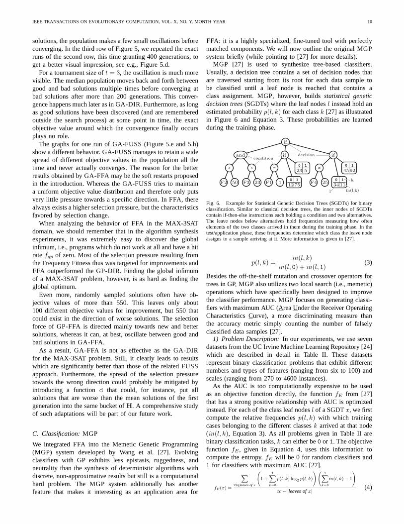
MGP [27] is used to synthesize tree-based classifiers.Usually, a decision tree contains a set of decision nodes thatare traversed starting from its root for each data sample tobe classified until a leaf node is reached that contains aclass assignment. MGP, however, buildsstatistical geneticdecision trees(SGDTs) where the leaf nodesl instead hold anestimated probabilityp(l, k) for each classk [27] as illustratedin Figure 6 and Equation 3. These probabilities are learnedduring the training phase.
Fig. 6. Example for Statistical Genetic Decision Trees (SGDTs) for binaryclassification. Similar to classical decision trees, the inner nodes of SGDTscontain if-then-else instructions each holding a condition and two alternatives.The leave nodes below alternatives hold frequencies measuring how oftenelements of the two classes arrived in them during the training phase. In thetest/application phase, these frequencies determine whichclass the leave nodeassigns to a sample arriving at it. More information is given in[27].
p(l, k) =in(l, k)
in(l, 0) + in(l, 1)(3)
Besides the off-the-shelf mutation and crossover operators fortrees in GP, MGP also utilizes two local search (i.e., memetic)operations which have specifically been designed to improvethe classifier performance. MGP focuses on generating classi-fiers with maximum AUC (Area Under the Receiver OperatingCharacteristics Curve), a more discriminating measure thanthe accuracy metric simply counting the number of falselyclassified data samples [27].
1) Problem Description:In our experiments, we use sevendatasets from the UC Irvine Machine Learning Repository [24]which are described in detail in Table II. These datasetsrepresent binary classification problems that exhibit differentnumbers and types of features (ranging from six to 100) andscales (ranging from 270 to 4600 instances).
As the AUC is too computationally expensive to be usedas an objective function directly, the functionfE from [27]that has a strong positive relationship with AUC is optimizedinstead. For each of the class leaf nodesl of a SGDTx, we firstcompute the relative frequenciesp(l, k) with which trainingcases belonging to the different classesk arrived at that node(in(l, k), Equation 3). As all problems given in Table II arebinary classification tasks,k can either be0 or 1. The objectivefunction fE , given in Equation 4, uses this information tocompute the entropy.fE will be 0 for random classifiers and1 for classifiers with maximum AUC [27].
fE(x) =
∑
∀l∈leaves ofx
(1 +
1∑
k=0
p(l, k) log2 p(l, k)
)(1∑
k=0
in(l, k)− 1
)
tc− |leaves ofx|(4)

IEEE TRANSACTIONS ON EVOLUTIONARY COMPUTATION, VOL. X, NO. Y, MONTH YEAR 11
Table IIDATA SETS [24] USED FOR THE CLASSIFICATION EXPERIMENTS. For each of the 7 data sets, we provide the shortcut and name, the number of instances,
the class distribution (0/1), a short summary on the features,and a reference to the corresponding literature.
Name Instances (Distribution) Features Referencebands Cylinder Bands 512 (312/200) 39: 19 nominal, 20 continuous [36]crx Credit Approval 690 (307/383) 15: 9 nominal, 6 continuous, some missing [37]
heart Statlog (Heart) 270 (150/120) 13: 3 binary, 1 ordered, 3 nominal, 6 continuous [38]hv Hill-Valley (both training sets) 1212 (612/600) 100 continuous [39]
mammo Mammographic Mass 961 (516/445) 6 integer/nominal, some missing [40]monks MONK’s Problem #1 (test sets) 432 (216/216) 6 integer (+ 1 id) [41]spam Spambase 4601 (2788/1813) 48 continuous [42]
Fig. 7.a: AUC performance on the training data.
Fig. 7.b: AUC performance on the test data.
Fig. 7. Box plots of the AUC of MGP-FFA and MGP-DIR over 100 runs (≡20 × five-fold cross-validation). Whereas MGP-DIR tends to perform betteron the training data (Figure 7.a, FFA seemingly decreased theoverfitting andimproved the diversity of the evolved classifiers, so that theperformance onthe test data (Figure 7.b) is very similar.
2) Experimental Settings:At first, we run the experimentswith the original algorithm, here denoted as MGP-DIR. Wethen directly introduce FFA into the MGP source code,replacing all accesses to the objective function with accesses tothe mapH, yielding algorithm MGP-FFA. In the experiments,we apply the dynamic stopping criterion of the latest MGPrelease that terminates the procedure if, after more than 50generations, no further improvement in terms of fitness couldbe achieved for ten generations and the AUC on the trainingdata is 1. All further algorithm settings are the same as in [27]and described in Table I.
3) Experimental Results:In Figure 7, we sketch the Boxplots of the classification experiment for the final achievedresults in terms of AUC on the training data (Figure 7.a) andtest data (Figure 7.b).
There is a small advantage of MGP-DIR over MGP-FFAon the training data and MGP-FFA has a much wider spreadof obtained solution quality – for the worse, that is. Themedians and quartiles on the test data, however, are oftenabout the same. In themonks problem, the 25% quan-
tile of MGP-FFA already reaches an AUC of 1, whereasMGP-DIR’s 25% quantile and median are 0.90 and 0.99,respectively. On the test data, MGP-DIR significantly out-performed MGP-FFA inbands and heart, MGP-FFAdelivers significantly better results inmonks, while there isno significant difference in the remaining datasets, accordingto two-tailed Mann-Whitney U test at significance level 0.02.
Although the performance of MGP-FFA on the test datais not much different from MGP-DIR, it produces morediverse classifiers with less overfitting – a wider spread oftraining AUC maps to basically the same range of test AUC.This makes MGP-FFA an interesting option for synthesizingensemble classifiers where diversity is favorable [43]. In sum-mary, FFA can indeed be used as a replacement for a directfitness measure – even in a highly specialized and complexsystem such as MGP.
D. Numerical Optimization: (1+1) ES
FFA intuitively seems to only be suitable for problemswith discrete objective values and indeed, all the previousexperiments were of this type. In this section we presenta straightforward extension to continuous optimization. Weassume the minimization of continuous,m-dimensional func-tions fi : R
m 7→ [0,+∞) on a computer with limitedprecision.2
If the computations are done with IEEE 754 double pre-cision floating point numbers [44], the range of positivefinite representable values spans from roughly 4.9· 10−324 to1.8· 10308. As ⌊ln(4.9 · 10−324)⌋ = −745, one possible wayto discretize such values into a tractable interval would betoapply the mappingd given in Equation 5.
d (y) =
{746 + round(ln(y)) if y > 0
0 otherwise(5)
As ⌈ln(1.8 · 10308)⌉ = 710, all possible outputs off canbe discretized into the interval0. . .1456, i.e., the FrequencyFitness mapping can be maintained as a lookup table with atmost 1457 entries.
1) Experimental Settings:To evaluate whether FFA canactually be applied in such a crude way to numerical opti-mization, we chose a well-studied algorithm as basis for ourexperiments: The(1 + 1) Evolution Strategy (ES) with self-adaptation via the1/5th rule [28, 29]. This algorithm keepsthe best candidate solutionx⋆ discovered so far and in each
2Strictly speaking, this makes the problems discrete again. However, suchproblems are commonly regarded as continuous.
IEEE TRANSACTIONS ON EVOLUTIONARY COMPUTATION, VOL. X, NO. Y, MONTH YEAR 12
generation generates one new vector by adding normally-distributed random numbers (mean0, standard deviationσ)to the elements ofx⋆. The outcome is accepted if it has betteror the same fitness asx⋆.
The step widthσ is initially set to σ0 = 1 and adaptedeveryL function evaluations (FEs), here withL ∈ {10, 100}.The adaptation setsσ = σ ∗ a if less than20% = 1/5 of themutation aresuccessful, i.e., leading tofitnessimprovementsduring the lastL steps and toσ = σ/a otherwise, wherea ∈ {0.5, 0.85, 0.975}. We chose the(1 + 1) ES because ofits simplicity, the mature state of the research on it, and formaximum replicability of experiments. We will refer to theoriginal form of this algorithm as ES-DIR.
We apply ES-DIR to eleven benchmark functions (seeTable III) for dimensions3 m ranging from1 to 5 in the interval[−10, 10]. We perform 100 runs for each setting and collect thebest results obtained per run afterFE = 10t with t ∈ 2 . . . 7FEs.
We then substitute FFA for the original objective functioninto the algorithm and repeat the experiments. We will callthe modified algorithm ES-FFA. Notice that the substitutionof FFA for the objective function will also affect the definitionof successwhich now means generating a candidate solutionwith a less-often discovered scale of fitness compared to thecurrently best solution.
2) Experimental Results:In this experiment, the resultsare quite clear. Similar to the MAX-3SAT experiments, nota single ES-FFA configuration can strictly outperform thecorresponding ES-DIR setting on any function. However,some settings come quite close: Form = 5 dimensions atFE = 105, 106, or 107 with L = 10 anda = 0.975, ES-FFAmanages to provide statistically significantly better resultsthan ES-DIR on three functions while being worse at four(according to two-tailed Mann-Whitney U test at significancelevel 0.02). The best ES-DIR setting withL = 100 anda = 0.5 outperforms all other settings 1944 times, loses 361times, and is not significantly different 1259 times, over allfunctions, dimensions, andFE settings. The best ES-FFAsetting (L = 10 and a = 0.975), in turn outperforms theother settings 1568 times, is not different 1094 times, and loses902 times – thus being better than one third of the ES-DIRsettings.
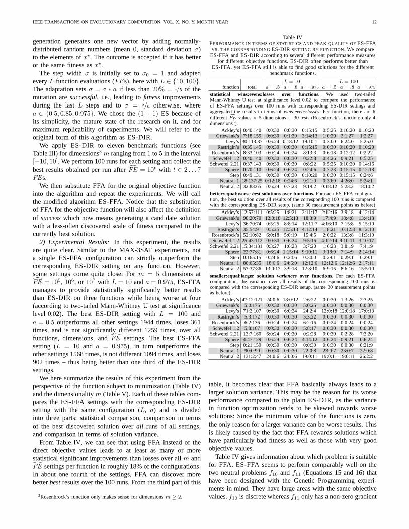
We here summarize the results of this experiment from theperspective of the function subject to minimization (TableIV)and the dimensionalitym (Table V). Each of these tables com-pares the ES-FFA settings with the corresponding ES-DIRsetting with the same configuration (L, a) and is dividedinto three parts: statistical comparison, comparison in termsof the best discovered solution overall runs of all settings,and comparison in terms of solution variance.
From Table IV, we can see that using FFA instead of thedirect objective values leads to at least as many or morestatistical significant improvements than losses over allm andFE settings per function in roughly 18% of the configurations.In about one fourth of the settings, FFA can discover morebetterbestresults over the 100 runs. From the third part of this
3Rosenbrock’s function only makes sense for dimensionsm ≥ 2.
Table IVPERFORMANCE IN TERMS OF STATISTICS AND PEAK QUALITY OFES-FFAVS. THE CORRESPONDINGES-DIR SETTING BY FUNCTION. We compareES-FFA and ES-DIR according to several different performance measures
for different objective functions. ES-DIR often performs better thanES-FFA, yet ES-FFA still is able to find good solutions for thedifferent
benchmark functions.
L = 10 L = 100function total a = .5 a = .8 a = .975 a = .5 a = .8 a = .975
statistical wins:evens:losses over functions. We used two-tailedMann-Whitney U test at significance level 0.02 to compare the performanceof ES-FFA settings over 100 runs with corresponding ES-DIR settings andaggregated the results in terms ofwins:evens:losses. Per function, there are 6different FE values× 5 dimensions≡ 30 tests (Rosenbrock’s function: only 4dimensions3).
Ackley’s 0:40:140 0:0:30 0:0:30 0:15:15 0:5:25 0:10:20 0:10:20Griewank’s 7:18:155 0:0:30 0:1:29 3:14:13 1:0:29 2:1:27 1:2:27
Levy’s 30:113:37 0:6:24 0:18:12 19:10:1 0:30:0 6:24:0 5:25:0Rastrigin’s 0:35:145 0:0:30 0:0:30 0:15:15 0:0:30 0:10:20 0:10:20
Rosenbrock’s 8:33:103 0:0:24 0:0:24 8:13:3 0:6:18 0:12:12 0:2:22Schwefel 1.2 0:40:140 0:0:30 0:0:30 0:22:8 0:4:26 0:9:21 0:5:25
Schwefel 2.21 0:37:143 0:0:30 0:0:30 0:8:22 0:5:25 0:10:20 0:14:16Sphere 0:70:110 0:6:24 0:6:24 0:24:6 0:7:23 0:15:15 0:12:18
Step 0:49:131 0:0:30 0:0:30 0:10:20 0:0:30 0:15:15 0:24:6Neutral 1 18:137:25 0:12:18 0:24:6 9:21:0 0:30:0 4:26:0 5:24:1Neutral 2 32:83:65 0:6:24 0:7:23 9:19:2 0:18:12 5:23:2 18:10:2
better:equal:worse bestsolutions over functions.For each ES-FFA configura-tion, the best solution over all results of the corresponding 100 runs is comparedwith the corresponding ES-DIR setup. (same 30 measurement points as before)
Ackley’s 12:57:111 0:5:25 1:8:21 2:11:172:12:16 3:9:18 4:12:14Griewank’s 90:20:70 12:0:18 12:5:13 18:3:9 17:4:9 18:4:8 13:4:13
Levy’s 36:70:74 0:5:25 8:8:14 12:11:74:16:10 7:15:8 5:15:10Rastrigin’s 35:54:91 0:5:25 12:5:13 4:12:14 1:8:21 10:12:8 8:12:10
Rosenbrock’s 52:10:82 6:0:18 5:0:19 15:4:5 2:0:22 13:3:8 11:3:10Schwefel 1.225:43:112 0:0:30 0:6:24 9:5:16 4:12:14 9:10:11 3:10:17
Schwefel 2.2115:34:131 0:3:27 1:6:23 3:7:20 1:6:23 3:8:19 7:4:19Sphere 22:77:81 0:6:24 1:15:14 9:10:11 3:18:9 7:14:9 2:14:14
Step 0:165:15 0:24:6 0:24:6 0:30:0 0:29:1 0:29:1 0:29:1Neutral 1 80:65:35 18:6:6 24:6:0 12:12:6 12:12:6 12:12:6 2:17:11Neutral 2 57:37:86 13:0:17 3:9:18 12:8:10 6:9:15 8:6:16 15:5:10
smaller:equal:larger solution variances over functions. For each ES-FFAconfiguration, the variance over all results of the corresponding 100 runs iscompared with the corresponding ES-DIR setup. (same 30 measurement pointsas before)
Ackley’s 47:12:121 24:0:6 18:0:12 2:6:22 0:0:30 1:3:26 2:3:25Griewank’s 5:0:175 0:0:30 0:0:30 5:0:25 0:0:30 0:0:30 0:0:30
Levy’s 71:2:107 0:0:30 6:0:24 24:2:4 12:0:18 12:0:18 17:0:13Rastrigin’s 5:3:172 0:0:30 0:0:30 5:3:22 0:0:30 0:0:30 0:0:30
Rosenbrock’s 6:2:136 0:0:24 0:0:24 6:2:16 0:0:24 0:0:24 0:0:24Schwefel 1.2 5:8:167 0:0:30 0:0:30 5:8:17 0:0:30 0:0:30 0:0:30
Schwefel 2.21 13:7:160 6:0:24 0:0:30 0:2:28 0:0:30 0:2:28 7:3:20Sphere 4:47:129 0:6:24 0:6:24 4:14:12 0:6:24 0:9:21 0:6:24
Step 0:21:159 0:0:30 0:0:30 0:0:30 0:0:30 0:0:30 0:21:9Neutral 1 90:0:90 0:0:30 0:0:30 22:0:8 23:0:7 23:0:7 22:0:8Neutral 2 131:2:47 24:0:6 24:0:6 19:0:1119:0:11 19:0:11 26:2:2
table, it becomes clear that FFA basically always leads to alarger solution variance. This may be the reason for its worseperformance compared to the plain ES-DIR, as the variancein function optimization tends to be skewed towards worsesolutions: Since the minimum value of the functions is zero,the only reason for a larger variance can be worse results. Thisis likely caused by the fact that FFA rewards solutions whichhave particularly bad fitness as well as those with very goodobjective values.
Table IV gives information about which problem is suitablefor FFA. ES-FFA seems to perform comparably well on thetwo neutral problemsf10 andf11 (Equations 15 and 16) thathave been designed with the Genetic Programming experi-ments in mind. They have large areas with the same objectivevalues.f10 is discrete whereasf11 only has a non-zero gradient

IEEE TRANSACTIONS ON EVOLUTIONARY COMPUTATION, VOL. X, NO. Y, MONTH YEAR 13
Table IIITHE ELEVEN NUMERICAL BENCHMARK FUNCTIONS. We define all benchmark functions used in the ES-FFA/ES-DIR experiments with their well-knownname, mathematical definition, and reference to literature (ifany). The two neutral poblems in Equations 15 and 16 have been designed for this study with
the Genetic Programming experiment (Section IV-A) in mind.
Ackley’s Function f1(x)=−20 exp(
−0.2√
1
m
∑m
i=1x2i
)
− exp(
1
m
∑m
i=1cos (2πxi)
)
+ 20 + e Eq. (6), see [25]
Griewank’s Function f2(x)=1
4000
∑m
i=1x2i −
∏m
i=1cos
(
xi√i
)
+ 1 Eq. (7), see [25]
Levy’s Function f3(x)= sin2 (πy1) +∑m−1
i=1(yi − 1)2 ·
[
1 + 10 sin2 (πyi + 1)]
+(yn − 1)2[
1 + sin2 (2 ∗ πxn)]
whereyi = 1 + xi−1
4
Eq. (8), see [26]
Rastrigin’s Function f4(x)=∑m
i=1
[
x2i − 10 cos (2πxi) + 10
]
Eq. (9), see [25]
Rosenbrock’s Function f5(x)=∑m−1
i=1
[
100(
xi+1 − x2i
)2+ (xi − 1)2
]
Eq. (10), see [25]
Schwefel’s Problem 1.2 f6(x)=∑n
i=1
(
∑i
j=1xi
)2
Eq. (11), see [25]
Schwefel’s Problem 2.21 f7(x)=maxi∈1...m {|xi|} Eq. (12), see [25]Sphere Function f8(x)=
∑n
i=1x2i Eq. (13), see [25]
Step Function f9(x)=∑n
i=1(⌊xi + 0.5⌋)2 Eq. (14), see [25]
Neutral Problem 1 f10(x)=1
m
∑m
i=1sin2 ⌊ixi⌋
iEq. (15)
Neutral Problem 2 f11(x)=1
m
∑m
i=1
{
x2i if x2
i ≤ 1
i
1 otherwiseEq. (16)
Table VPERFORMANCE IN TERMS OF STATISTICS AND PEAK QUALITY OFES-FFA
VS. THE CORRESPONDINGES-DIR SETTING BY DIMENSIONm. Wecompare the ES-FFA and ES-DIR for rising function dimensionsm andfind that ES-FFA tends to lose more comparisons with risingm, likely
because of an increasing span of possible objective values.
L = 10 L = 100m total a = .5 a = .8 a = .975 a = .5 a = .8 a = .975
statistical wins:evens:losses over dimensions.We used two-tailedMann-Whitney U test at significance level 0.02 to compare the performanceof ES-FFA settings over 100 runs with corresponding ES-DIR settings andaggregated the results in terms ofwins:evens:losses. Per dimension, there are6 different FE values× 11 functions≡ 66 tests (Rosenbrock’s function:only 4 dimensions3).
1 18:192:150 0:18:42 0:25:35 8:40:12 1:34:25 3:38:19 6:37:172 22:154:220 0:12:54 0:12:54 8:42:16 0:22:44 4:37:25 10:29:273 20:136:240 0:0:66 0:12:54 10:37:190:19:47 5:36:25 5:32:294 18:95:283 0:0:66 0:6:60 9:31:26 0:12:54 5:26:35 4:20:425 17:78:301 0:0:66 0:1:65 13:21:320:18:48 0:18:48 4:20:42
better:equal:worse best solutions over dimensions.For each ES-FFAconfiguration, the best solution over all results of the corresponding 100 runsis compared with the corresponding ES-DIR setup. (same 66 measurementpoints as before.)
1 86:206:68 13:30:17 12:40:8 19:32:9 13:38:9 13:34:13 16:32:122 112:158:126 18:6:42 25:26:15 21:27:18 12:35:19 17:33:16 19:31:163 88:135:173 12:6:48 12:17:37 19:24:2310:29:27 21:28:17 14:31:214 48:88:260 0:12:54 6:9:51 18:18:30 3:16:47 16:15:35 5:18:435 90:45:261 6:0:60 12:0:54 19:12:3514:8:44 23:12:31 16:13:37
smaller:equal:larger solution variances over dimensions. For eachES-FFA configuration, the variance over all results of the corresponding100 runs is compared with the corresponding ES-DIR setup. (same 66measurement points as before.)
1 56:62:242 6:6:48 6:6:48 11:17:3212:6:42 8:11:41 13:16:312 94:14:288 12:0:54 12:0:54 24:8:34 13:0:53 13:0:53 20:6:403 71:14:311 12:0:54 6:0:60 17:6:43 11:0:55 11:3:52 14:5:474 88:8:300 12:0:54 12:0:54 23:4:39 12:0:54 12:0:54 17:4:455 68:6:322 12:0:54 12:0:54 17:2:47 6:0:60 11:0:55 10:4:52
in a small area of the search space. During 100 runs, ES-FFAalso discovered better best results on Levy’s and Griewank’sfunction more often than ES-DIR.
Table V shows that with rising dimensionalitym of the ob-jective functions, there is a clear trend towards more statisticallosses of ES-FFA to ES-DIR. The reason for this maybe isthat the span width of different possible objective values for
the points within[−10, 10]m increases withm and so does thenumber of entries in the frequency table that are used. Thisprobably disperses the selection pressure.
3) Behavior of FFA:We now show how FFA works withinES-FFA forL = 10 anda = 0.975.
a) Sphere Function:As the first example we chose theSphere function (f8 in Table III) because of its simplicity. InFigure 8, we illustrate the Sphere function itself (Figure 8.a).This function is unimodal, smooth, and symmetric around0,so we can also plot one half of it by using a logarithmic scalefor x (right part of the subfigure).
In the second plot (Figure 8.b), the trace of a typical run ofES-FFA onf8 is shown. On the x-axis, we plot the functionevaluationFE . The y-axis is logarithmically scaled. We showthe distance of the pointx sampled by the ES-FFA at aspecificFE to the global optimum0, i.e., |x|. It can be seenthat this distance tends to get smaller in scale. The(1 + 1)-ES always holds the best pointx⋆ found so far, and forES-FFA, best is defined in terms of the Frequency Fitness.With the thick black line, we illustrate|x⋆|. As it can be seen,this value also tends to get logarithmically smaller, but notmonotonically – FFA here sometimes prefers to make a stepback. We also plotf8(x⋆) which (due tof8(x) = x2) hasthe same characteristics. The1/5th rule leads to a monotonousdecrease in scale ofσ.
The shape of this run thus is very similar to what weget from ES-DIR. We now investigate how the frequencyinformationH [d ( · )] within the ES-FFA is constructed andtherefore plot the frequency table at four distinct functionevaluations (FE∈ {10, 100, 1000, 10000} in Figures 8.c to 8.f.Each subfigure has two parts, on the left side we plotH [d (f8(x))] over the whole search spacex ∈ [−10, 10]. Onthe right side, we use a logarithmically scaled x-axis from10−18 to 10 (as f8 is symmetric, i.e.,f8(x) = f8(−x) =f8(|x|), we can join the positive and negative side into onediagram by plotting values for|x|).
After sampling ten points (Figure 8.c), high absolute valuesof x (and thus,f8) have been discovered around five times,

IEEE TRANSACTIONS ON EVOLUTIONARY COMPUTATION, VOL. X, NO. Y, MONTH YEAR 14
Fig. 8.a: The shape of the Sphere function (f8). Fig. 8.b: The trace of a typical ES-FFA run onf8.
Fig. 8.c: The frequency state of that run after 10FEs. Fig. 8.d: The frequency state of that run after 100FEs.
Fig. 8.e: The frequency state of that run after 1000FEs. Fig. 8.f: The frequency state of that run after 10000FEs.
Fig. 8. Behavior of FFA on the Sphere function (f8). Here we illustrate the behavior of a typical run of ES-FFA when optimizing the Sphere function(heref8) plotted in Figure 8.a. Figure 8.b shows how the search progresses in terms of solution quality whereas Figures 8.c to 8.f illustrate the contents ofthe frequency tableH after different numbers function evaluations.
whereas the area around the optimum has not yet beensampled. Together with the worst possible areas on the bordersof the search space, there are three undiscovered local optimain the frequency landscape.
After 100 FEs (Figure 8.d), the frequency landscape nowlooks very different from the originalf8. ES-FFA has en-tered the area round0 and sampled many points around it,which created two big walls dividing it from the rest ofthe search space. If we remember that objective values arediscretized logarithmically (see Equation 5) and thatσ isconstantly reduced due to self-adaptation, the right side ofthe plot gives better information. From the perspective of theES-FFA, |x| ∈ [1, 10] would be interesting, but is dividedfrom the currentx⋆ by walls of solutions with very bad fitness(|x| ∈ [0.1, 1]). On the left side of these solutions, however,there is a large local optimum, a (logarithmically) big spaceof solutions with a zero frequency.
This pool is now explored during the remainingFEs (Fig-ures 8.e and 8.f). Whenever ES-FFA samples a point, it caneither be in the unexplored area closer to the global optimum(thus having a low frequency), or on the wall separating theoutside of the search space – hence having a bad fitness. Thesearch is driven towards the global optimum0. It samples
many objective values of smaller and smaller scale, makingthe wall to the outside of the search space wider and wider.
b) Ackley’s Function:On Ackley’s function (f1 in Ta-ble III), we illustrate an example run where FFA correctsthe direction of the search. In Figure 9, we first plot theshape of Ackley’s function (Figure 9.a) and the first 100function evaluations of a typical run (Figure 9.b).f1 issymmetric around its global optimum0. The illustrated runstarts with a random initial point around 5, then searches inthe wrong direction (towards 10) for some time, until it beginsto converge towards the global optimum after around 30FEs.
The four plots in Figures 9.c to 9.f illustrate the aggregatedfrequency information for 10, 15, 20, and 50FEs. It can beseen that after 10FEs, there are three large locally optimalareas in the frequency landscape: around the true globaloptimum0 and around both ends of the search space. ES-FFAthen explores the upper end of the search space. The objectivevalues of this area, due to logarithmic discretization, largelyfall into the same frequency table index and thus quicklydegenerate in fitness (Figures 9.d and 9.e). Only the center arearemains as the global optimum in the frequency landscape.Starting at around 50FEs, ES-FFA again aggregates wallsaround this locally optimal area. The algorithm now behaves

IEEE TRANSACTIONS ON EVOLUTIONARY COMPUTATION, VOL. X, NO. Y, MONTH YEAR 15
Fig. 9.a: The shape of Ackley’s function (f1). Fig. 9.b: The trace of a typical ES-FFA run onf1.
Fig. 9.c: The frequency state of that run after 10FEs. Fig. 9.d: The frequency state of that run after 15FEs.
Fig. 9.e: The frequency state of that run after 20FEs. Fig. 9.f: The frequency state of that run after 50FEs.
Fig. 9. Behavior of FFA on Ackley’s function (f1). Here we illustrate the behavior of a typical run of ES-FFA when optimizing the Ackley’s function(heref1) plotted in Figure 9.a. Figure 9.b shows how the search progresses in terms of solution quality whereas Figures 9.c to 9.f illustrate the contents ofthe frequency tableH after different numbers function evaluations.
exactly in the way that we already observed for the Spherefunction in the previous section. This makes sense, as in theright part of Figure 9.a, we see that the logarithmic-scale shapeof Ackley’s function is actually quite similar to the Spherefor|x| < 1.
c) Discussion: We analyzed ES-FFA with plots onmultiple benchmark functions and generally observed thebehaviors discussed in the previous section. In most of the runsthat we plotted, the behavior and convergence of ES-FFA isvery similar to ES-DIR.
In some cases, however, ES-FFA would prematurely con-verge, which accounts for its worse overall performance. Thisseems to be puzzling, as FFA is a technique devised exactlyto prevent this. The reason is that the1/5th rule prescribes thatthe mutation step width should be decreased when too manymutations fail. If this happens too early andσ gets so smallthat no points outside the current “bucket”d ( · ) of H can besampled anymore, mutation will no longer succeed andσ willcontinue to be decreased. We observe this effect especiallywith low settings forL anda and even more under the moreaggressive adaptation rule given in [45].
Some methodd to discretize the objective values is nec-essary if FFA is applied to a continuous problem – there
can only be finitely many indices for the tableH. Thisexperiment here emphasizes the influence ofd. The static,logarithm-based approach given in Equation 5 clashes withthe self-adaptation of the ES. If future applications of FFAforcontinuous optimization are to be competitive, it is necessaryto either devise better mappings, to develop a new approachnot needing a tableH, or to apply other methods like NoveltySearch [1, 2] that do not have this requirement in the firstplace instead.
V. CONCLUSIONS
In this paper, we introduced FFA as a new fitness assign-ment method and showed that it(a) can self-adaptively andsmoothly switch between exploration and exploitation,(b) cansignificantly improve the solution quality,(c) can increase thesolution diversity, and(d) can be integrated both into basicmetaheuristics as well as into complicated existing optimiza-tion systems in a straightforward way (see Section IV-C).
We found that it performs particularly well on problemswhere most randomly sampled candidate solutions have badobjective values. In the Genetic Programming experiment(Section IV-A), where the objective function is very ruggedand there is a high degree of epistasis in the search space,
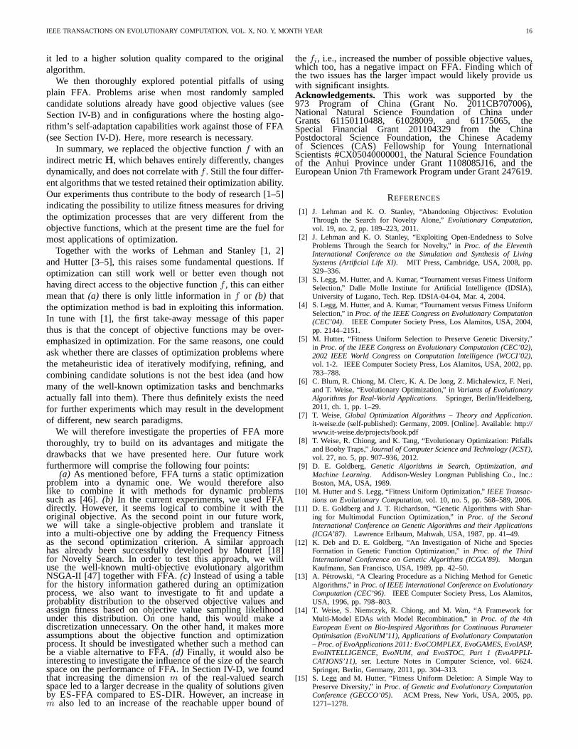
IEEE TRANSACTIONS ON EVOLUTIONARY COMPUTATION, VOL. X, NO. Y, MONTH YEAR 16
it led to a higher solution quality compared to the originalalgorithm.
We then thoroughly explored potential pitfalls of usingplain FFA. Problems arise when most randomly sampledcandidate solutions already have good objective values (seeSection IV-B) and in configurations where the hosting algo-rithm’s self-adaptation capabilities work against those of FFA(see Section IV-D). Here, more research is necessary.
In summary, we replaced the objective functionf with anindirect metricH, which behaves entirely differently, changesdynamically, and does not correlate withf . Still the four differ-ent algorithms that we tested retained their optimization ability.Our experiments thus contribute to the body of research [1–5]indicating the possibility to utilize fitness measures for drivingthe optimization processes that are very different from theobjective functions, which at the present time are the fuel formost applications of optimization.
Together with the works of Lehman and Stanley [1, 2]and Hutter [3–5], this raises some fundamental questions. Ifoptimization can still work well or better even though nothaving direct access to the objective functionf , this can eithermean that(a) there is only little information inf or (b) thatthe optimization method is bad in exploiting this information.In tune with [1], the first take-away message of this paperthus is that the concept of objective functions may be over-emphasized in optimization. For the same reasons, one couldask whether there are classes of optimization problems wherethe metaheuristic idea of iteratively modifying, refining,andcombining candidate solutions is not the best idea (and howmany of the well-known optimization tasks and benchmarksactually fall into them). There thus definitely exists the needfor further experiments which may result in the developmentof different, new search paradigms.
We will therefore investigate the properties of FFA morethoroughly, try to build on its advantages and mitigate thedrawbacks that we have presented here. Our future workfurthermore will comprise the following four points:
(a) As mentioned before, FFA turns a static optimizationproblem into a dynamic one. We would therefore alsolike to combine it with methods for dynamic problemssuch as [46].(b) In the current experiments, we used FFAdirectly. However, it seems logical to combine it with theoriginal objective. As the second point in our future work,we will take a single-objective problem and translate itinto a multi-objective one by adding the Frequency Fitnessas the second optimization criterion. A similar approachhas already been successfully developed by Mouret [18]for Novelty Search. In order to test this approach, we willuse the well-known multi-objective evolutionary algorithmNSGA-II [47] together with FFA.(c) Instead of using a tablefor the history information gathered during an optimizationprocess, we also want to investigate to fit and update aprobablity distribution to the observed objective values andassign fitness based on objective value sampling likelihoodunder this distribution. On one hand, this would make adiscretization unnecessary. On the other hand, it makes moreassumptions about the objective function and optimizationprocess. It should be investigated whether such a method canbe a viable alternative to FFA.(d) Finally, it would also beinteresting to investigate the influence of the size of the searchspace on the performance of FFA. In Section IV-D, we foundthat increasing the dimensionm of the real-valued searchspace led to a larger decrease in the quality of solutions givenby ES-FFA compared to ES-DIR. However, an increase inm also led to an increase of the reachable upper bound of
the fi, i.e., increased the number of possible objective values,which too, has a negative impact on FFA. Finding which ofthe two issues has the larger impact would likely provide uswith significant insights.Acknowledgements. This work was supported by the973 Program of China (Grant No. 2011CB707006),National Natural Science Foundation of China underGrants 61150110488, 61028009, and 61175065, theSpecial Financial Grant 201104329 from the ChinaPostdoctoral Science Foundation, the Chinese Academyof Sciences (CAS) Fellowship for Young InternationalScientists #CX05040000001, the Natural Science Foundationof the Anhui Province under Grant 1108085J16, and theEuropean Union 7th Framework Program under Grant 247619.
REFERENCES
[1] J. Lehman and K. O. Stanley, “Abandoning Objectives: EvolutionThrough the Search for Novelty Alone,”Evolutionary Computation,vol. 19, no. 2, pp. 189–223, 2011.
[2] J. Lehman and K. O. Stanley, “Exploiting Open-Endedness to SolveProblems Through the Search for Novelty,” inProc. of the EleventhInternational Conference on the Simulation and Synthesis of LivingSystems (Artificial Life XI). MIT Press, Cambridge, USA, 2008, pp.329–336.
[3] S. Legg, M. Hutter, and A. Kumar, “Tournament versus Fitness UniformSelection,” Dalle Molle Institute for Artificial Intelligence (IDSIA),University of Lugano, Tech. Rep. IDSIA-04-04, Mar. 4, 2004.
[4] S. Legg, M. Hutter, and A. Kumar, “Tournament versus Fitness UniformSelection,” inProc. of the IEEE Congress on Evolutionary Computation(CEC’04). IEEE Computer Society Press, Los Alamitos, USA, 2004,pp. 2144–2151.
[5] M. Hutter, “Fitness Uniform Selection to Preserve Genetic Diversity,”in Proc. of the IEEE Congress on Evolutionary Computation (CEC’02),2002 IEEE World Congress on Computation Intelligence (WCCI’02),vol. 1-2. IEEE Computer Society Press, Los Alamitos, USA, 2002, pp.783–788.
[6] C. Blum, R. Chiong, M. Clerc, K. A. De Jong, Z. Michalewicz,F. Neri,and T. Weise, “Evolutionary Optimization,” inVariants of EvolutionaryAlgorithms for Real-World Applications. Springer, Berlin/Heidelberg,2011, ch. 1, pp. 1–29.
[7] T. Weise, Global Optimization Algorithms – Theory and Application.it-weise.de (self-published): Germany, 2009. [Online]. Available: http://www.it-weise.de/projects/book.pdf
[8] T. Weise, R. Chiong, and K. Tang, “Evolutionary Optimization: Pitfallsand Booby Traps,”Journal of Computer Science and Technology (JCST),vol. 27, no. 5, pp. 907–936, 2012.
[9] D. E. Goldberg, Genetic Algorithms in Search, Optimization, andMachine Learning. Addison-Wesley Longman Publishing Co., Inc.:Boston, MA, USA, 1989.
[10] M. Hutter and S. Legg, “Fitness Uniform Optimization,”IEEE Transac-tions on Evolutionary Computation, vol. 10, no. 5, pp. 568–589, 2006.
[11] D. E. Goldberg and J. T. Richardson, “Genetic Algorithmswith Shar-ing for Multimodal Function Optimization,” inProc. of the SecondInternational Conference on Genetic Algorithms and their Applications(ICGA’87). Lawrence Erlbaum, Mahwah, USA, 1987, pp. 41–49.
[12] K. Deb and D. E. Goldberg, “An Investigation of Niche andSpeciesFormation in Genetic Function Optimization,” inProc. of the ThirdInternational Conference on Genetic Algorithms (ICGA’89). MorganKaufmann, San Francisco, USA, 1989, pp. 42–50.
[13] A. Petrowski, “A Clearing Procedure as a Niching Method for GeneticAlgorithms,” in Proc. of IEEE International Conference on EvolutionaryComputation (CEC’96). IEEE Computer Society Press, Los Alamitos,USA, 1996, pp. 798–803.
[14] T. Weise, S. Niemczyk, R. Chiong, and M. Wan, “A Framework forMulti-Model EDAs with Model Recombination,” inProc. of the 4thEuropean Event on Bio-Inspired Algorithms for Continuous ParameterOptimisation (EvoNUM’11), Applications of Evolutionary Computation– Proc. of EvoApplications 2011: EvoCOMPLEX, EvoGAMES, EvoIASP,EvoINTELLIGENCE, EvoNUM, and EvoSTOC, Part 1 (EvoAPPLI-CATIONS’11), ser. Lecture Notes in Computer Science, vol. 6624.Springer, Berlin, Germany, 2011, pp. 304–313.
[15] S. Legg and M. Hutter, “Fitness Uniform Deletion: A Simple Way toPreserve Diversity,” inProc. of Genetic and Evolutionary ComputationConference (GECCO’05). ACM Press, New York, USA, 2005, pp.1271–1278.

IEEE TRANSACTIONS ON EVOLUTIONARY COMPUTATION, VOL. X, NO. Y, MONTH YEAR 17
[16] J. Lehman and K. O. Stanley, “Evolving a Diversity of Virtual CreaturesThrough Novelty Search and Local Competition,” inProc. of the Geneticand Evolutionary Computation Conference (GECCO’11), 2011, pp.211–218.
[17] G. Cuccu, F. Gomez, and T. Glasmachers, “Novelty-Based Restartsfor Evolution Strategies,” inProc. of the 12th IEEE Congress onEvolutionary Computation (CEC’11), 2011, pp. 158–163.
[18] J. Mouret, “Novelty-based Multiobjectivization,” inNew Horizonsin Evolutionary Robotics – Extended Contributions from the2009EvoDeRob Workshop (EvoDeRob’09), ser. Studies in ComputationalIntelligence, vol. 341. Springer, Berlin/Heidelberg, 2009, pp. 139–154.
[19] F. Glover, E. D. Taillard, and D. de Werra, “A User’s Guide to TabuSearch,”Annals of Operations Research, vol. 41, no. 1, pp. 3–28, 1993.
[20] A. Hertz, E. D. Taillard, and D. de Werra, “A Tutorial on TabuSearch,” inGiornate di Lavoro (Entreprise Systems: Management ofTechnological and Organizational Changes, “Gestione del cambiamentotecnologico ed organizzativo nei sistemi d’impresa”) (AIRO’95). Op-timization and Decision Sciences (AIRO), 1995, pp. 13–24.
[21] M. Wan, T. Weise, and K. Tang, “Novel Loop Structures andtheEvolution of Mathematical Algorithms,” inProc. of the 14th EuropeanConference on Genetic Programming (EuroGP’11), ser. Lecture Notesin Computer Science, vol. 6621/2011. Springer, Berlin, Germany, 2011,pp. 49–60.
[22] H. H. Hoos and T. Stutzle, “SATLIB – The Satisfiability Library,” 2005.[Online]. Available: http://www.cs.ubc.ca/∼hoos/SATLIB/benchm.html
[23] H. H. Hoos and T. Stutzle, “SATLIB: An Online Resource for Researchon SAT,” in SAT2000 – Highlights of Satisfiability Research in the Year2000, ser. Frontiers in Artificial Intelligence and Applications. IOSPress, Amsterdam, The Netherlands, 2000, vol. 63, pp. 283–292.
[24] “UC Irvine Machine Learning Repository.” [Online]. Available: http://archive.ics.uci.edu/ml/
[25] X. Yao, Y. Liu, and G. Lin, “Evolutionary Programming MadeFaster,”IEEE Transactions on Evolutionary Computation, vol. 3, no. 2, pp. 82–102, 1999.
[26] A. V. Levy and A. J. Montalvo, “The Tunneling Algorithm for the GlobalMinimization of Functions,”SIAM Journal of Scientific and StatisticalComputing, vol. 6, no. 1, pp. 15–29, 1985.
[27] P. Wang, K. Tang, E. P. K. Tsang, and X. Yao, “A Memetic GeneticProgramming with Decision Tree-Based Local Search for ClassificationProblems,” inProc. of the 12th IEEE Congress on Evolutionary Com-putation (CEC’11), 2011, pp. 917–924.
[28] H. Beyer and H. Schwefel, “Evolution Strategies – A ComprehensiveIntroduction,” Natural Computing: An International Journal, vol. 1,no. 1, pp. 3–52, 2002.
[29] H. Beyer,The Theory of Evolution Strategies, ser. Natural ComputingSeries. Springer, New York, USA, 2001.
[30] I. Rechenberg, “Evolutionsstrategie: Optimierung technischer Systemenach Prinzipien der biologischen Evolution,” Ph.D. dissertation, Tech-nische Universitat Berlin, Germany, 1971.
[31] T. Weise and K. Tang, “Evolving Distributed Algorithms with Ge-netic Programming,”IEEE Transactions on Evolutionary Computation,vol. 16, no. 2, pp. 242–265, 2012.
[32] J. R. Koza,Genetic Programming: On the Programming of Computersby Means of Natural Selection, ser. Bradford Books. MIT Press,Cambridge, USA, 1992.
[33] T. Weise, M. Zapf, and K. Geihs, “Rule-based Genetic Programming,”in Proc. of the 2nd International Conference on Bio-Inspired Models ofNetwork, Information, and Computing Systems (BIONETICS’07). IEEEComputer Society, Piscataway, USA, 2007, pp. 8–15.
[34] T. Weise, “Illustration of Statistical Test Results for ExperimentEvaluation,” University of Science and Technology of China(USTC),School of Computer Science and Technology, Nature InspiredComputation and Applications Laboratory (NICAL): Hefei, Anhuı,China, Tech. Rep., 2011. [Online]. Available: http://www.it-weise.de/documents/files/W2011IOSTRFEE.pdf
[35] S. B. Rana and L. D. Whitley, “Genetic Algorithm Behaviorin theMAXSAT Domain,” in Proc. of the 5th International Conference onParallel Problem Solving from Nature (PPSN V), ser. Lecture Notes inComputer Science, vol. 1498/1998. Springer, Berlin, Germany, 1998,pp. 785–794.
[36] B. Evans,Cylinder Bands Data Set. UCI Machine Learning Repository,Center for Machine Learning and Intelligent Systems, DonaldBrenSchool of Information and Computer Science, University of California:Irvine, CA, USA, 1995. [Online]. Available: http://archive.ics.uci.edu/ml/datasets/Cylinder+Bands
[37] Credit Approval Data Set. UCI Machine Learning Repository, Centerfor Machine Learning and Intelligent Systems, Donald Bren School
of Information and Computer Science, University of California:Irvine, CA, USA, 1987. [Online]. Available: http://archive.ics.uci.edu/ml/datasets/Credit+Approval
[38] Statlog (Heart) Data Set. UCI Machine Learning Repository, Centerfor Machine Learning and Intelligent Systems, Donald Bren Schoolof Information and Computer Science, University of California:Irvine, CA, USA, 1997. [Online]. Available: http://archive.ics.uci.edu/ml/datasets/Statlog+%28Heart%29
[39] L. Graham and F. Oppacher,Hill-Valley Data Set. UCI MachineLearning Repository, Center for Machine Learning and IntelligentSystems, Donald Bren School of Information and Computer Science,University of California: Irvine, CA, USA, 2008. [Online].Available:http://archive.ics.uci.edu/ml/datasets/Hill-Valley
[40] M. Elter and R. Schulz-Wendtland,Mammographic Mass Data Set.UCI Machine Learning Repository, Center for Machine Learning andIntelligent Systems, Donald Bren School of Information and ComputerScience, University of California: Irvine, CA, USA, 2007. [Online].Available: http://archive.ics.uci.edu/ml/datasets/Mammographic+Mass
[41] S. B. Thrun,MONK’s Problems Data Set. UCI Machine LearningRepository, Center for Machine Learning and Intelligent Systems,Donald Bren School of Information and Computer Science, Universityof California: Irvine, CA, USA, 1992. [Online]. Available:http://archive.ics.uci.edu/ml/datasets/MONK%27s+Problems
[42] M. Hopkins, E. Reeber, G. Forman, and J. Suermondt,Spambase DataSet. UCI Machine Learning Repository, Center for Machine Learningand Intelligent Systems, Donald Bren School of Information andComputer Science, University of California: Irvine, CA, USA, 1999.[Online]. Available: http://archive.ics.uci.edu/ml/datasets/Spambase
[43] L. I. Kuncheva and C. J. Whitaker, “Measures of Diversityin Classi-fier Ensembles and Their Relationship with the Ensemble Accuracy,”Machine Learning, vol. 51, no. 2, pp. 181–207, 2003.
[44] ANSI/IEEE Std 754-1985 – IEEE Standard for Binary Floating-PointArithmetic. IEEE, Piscataway, USA, 1985.
[45] A. Auger, “Benchmarking the (1+1) Evolution Strategy with One-FifthSuccess Rule on the BBOB-2009 Function Testbed,” inProc. of the11th Annual Conference on Genetic and Evolutionary Computation(GECCO’09). ACM, New York, USA, 2009, pp. 2447–2452.
[46] S. Yang, Y. Ong, and Y. Jin, Eds.,Evolutionary Computation in Dynamicand Uncertain Environments, ser. Studies in Computational Intelligence.Springer, Berlin/Heidelberg, 2007, vol. 51/2007.
[47] K. Deb, S. Agrawal, A. Pratab, and T. Meyarivan, “A Fast Elitist Non-Dominated Sorting Genetic Algorithm for Multi-Objective Optimization:NSGA-II,” in Proc. of the 6th International Conference on ParallelProblem Solving from Nature (PPSN VI), ser. Lecture Notes in ComputerScience, vol. 1917/2000. Springer, Berlin, Germany, 2000, pp. 849–858.
Thomas Weise(M’10) received the Diplom Infor-matiker (equivalent to M.Sc.) degree from the De-partment of Computer Science, Chemnitz Universityof Technology, Chemnitz, Germany, in 2005, andthe Ph.D. degree at the Distributed Systems Groupof the Fachbereich Elektrotechnik and Informatik,University of Kassel, Kassel, Germany in 2009.
In 2009, he took a position post-doctoral re-searcher at the School of Computer Science andTechnology, University of Science and Technologyof China (USTC), Hefei, China. Subsequently, in
2011, he was promoted to Associate Professor at USTC-Birmingham JointResearch Institute in Intelligent Computation and Its Applications (UBRI)which is part of the same school. His major research interests include planningfor logistics applications, Evolutionary Computation, Genetic Programming,and real-world applications of optimization algorithms. Hisexperience rangesfrom applying GP to distributed systems and multi-agent systems, efficientweb service composition for Service Oriented Architectures, to solvinglarge-scale real-world vehicle routing problems for multimodal logistics andtransportation.
Besides being the author/co-author of over 60 refereed publications, Dr.Weise also authors the electronic bookGlobal Optimization Algorithms –Theory and Applicationwhich is freely available at his website http://www.it-weise.de/.

IEEE TRANSACTIONS ON EVOLUTIONARY COMPUTATION, VOL. X, NO. Y, MONTH YEAR 18
Mingxu Wan Mingxu Wan graduated from theUSTC-Birmingham Joint Research Institute in In-telligent Computation and Its Applications (UBRI),School of Computer Science and Technology, Uni-versity of Science and Technology of China (USTC),Hefei, China in 2012 and pursued a carreer in thesoftware industry thereafter.
Ke Tang Ke Tang (S’05—M’07—SM’12) receivedthe B.Eng. degree from the Huazhong University ofScience and Technology, Wuhan, China, in 2002,and the Ph.D. degree from the School of Electricaland Electronic Engineering, Nanyang TechnologicalUniversity, Singapore, in 2007.
In 2007, he joined the USTC-Birmingham JointResearch Institute in Intelligent Computation and ItsApplications (UBRI), School of Computer Scienceand Technology, University of Science and Tech-nology of China (USTC), Hefei, China, and was
promoted to professor in 2011. He is also an Honorary Senior Research Fellowin the School of Computer Science, University of Birmingham, UK. He hasauthored/co-authored more than 50 refereed publications. His major researchinterests include evolutionary computation and machine learning. He is anassociate editor of IEEE Computational Intelligence Magazine and served asa program co-chair of CEC2010, held in Barcelona.
Pu Wang Pu Wang received the Bachelors degreein computer science from the University of Scienceand Technology of China (USTC), Hefei, China, in2008.
He is currently pursuing the Ph.D. degree fromthe USTC-Birmingham Joint Research Institutein Intelligent Computation and Its Applications(UBRI), School of Computer Science and Technol-ogy, USTC. His current research interests includeevolutionary computation, memetic algorithms, andmultiobjective optimization for classification prob-
lems in machine learning, and genetic programming for model checking insoftware engineering.
Alexandre Devert Alex, please provide me withsome input here.
Xin Yao (M’91—SM’96—F’03) is a Chair (Pro-fessor) of Computer Science at the University ofBirmingham, UK. He is the Director of CERCIA(the Centre of Excellence for Research in Com-putational Intelligence and Applications), Univer-sity of Birmingham, UK, and of the Joint USTC-Birmingham Research Institute of Intelligent Com-putation and Its Applications. He is an IEEE Fellowand a Distinguished Lecturer of IEEE ComputationalIntelligence Society (CIS). He won the 2001 IEEEDonald G. Fink Prize Paper Award, 2010 IEEE
Transactions on Evolutionary Computation Outstanding Paper Award, 2010BT Gordon Radley Award for Best Author of Innovation (Finalist), 2011IEEE Transactions on Neural Networks Outstanding Paper Award, and manyother best paper awards at conferences. He won the prestigious Royal SocietyWolfson Research Merit Award in 2012 and was selected to receive the 2013IEEE CIS Evolutionary Computation Pioneer Award. He was the Editor-in-Chief (2003-08) of IEEE Transactions on Evolutionary Computation. He hasbeen invited to give more than 65 keynote/plenary speeches atinternationalconferences in many different countries. His major research interests includeevolutionary computation and neural network ensembles. He has more than400 refereed publications in international journals and conferences. Accordingto Google Scholar, his H-index is 57 and total citations more than 17,000.
Related Documents