126 IEEE TRANSACTIONS ON EVOLUTIONARY ...atarazanas.sci.uma.es/docs/tesisuma/1661480x.pdf128 IEEE TRANSACTIONS ON EVOLUTIONARY COMPUTATION, VOL. 9, NO. 2, APRIL 2005 Fig. 2. Growth

126 IEEE TRANSACTIONS ON EVOLUTIONARY COMPUTATION, VOL. 9, NO. 2, APRIL 2005

The Exploration/Exploitation Tradeoff in DynamicCellular Genetic Algorithms

Enrique Alba and Bernabé Dorronsoro

Abstract—This paper studies static and dynamic decentralizedversions of the search model known as cellular genetic algorithm(cGA), in which individuals are located in a specific topology andinteract only with their neighbors. Making changes in the shapeof such topology or in the neighborhood may give birth to a highnumber of algorithmic variants. We perform these changes ina methodological way by tuning the concept of ratio. Since therelationship (ratio) between the topology and the neighborhoodshape defines the search selection pressure, we propose to analyzein depth the influence of this ratio on the exploration/exploitationtradeoff. As we will see, it is difficult to decide which ratio is bestsuited for a given problem. Therefore, we introduce a prepro-grammed change of this ratio during the evolution as a possibleadditional improvement that removes the need of specifying asingle ratio. A later refinement will lead us to the first adaptive dy-namic kind of cellular models to our knowledge. We conclude thatthese dynamic cGAs have the most desirable behavior among allthe evaluated ones in terms of efficiency and accuracy; we validateour results on a set of seven different problems of considerablecomplexity in order to better sustain our conclusions.

Index Terms—Cellular genetic algorithm (cGA), evolutionary al-gorithm (EA), dynamic adaptation, neighborhood-to-populationratio.

I. INTRODUCTION

THE APPLICATION of evolutionary algorithms (EAs)to optimization problems has been very intense during

the last decade [1]. It is possible to find this kind of algo-rithm applied for solving complex problems like constrainedoptimization tasks, problems with a noisy objective function,or problems having high epistasis and multimodality. Thesealgorithms work over a set (population) of potential solutions(individuals) by applying some stochastic operators on them inorder to search for the best solutions. Most EAs use a singlepopulation (panmixia) of individuals and apply operators onthem as a whole [see Fig. 1(a)]. In contrast, there exists alsosome tradition in using structured EAs (where the population isdecentralized somehow), especially in relation to their parallelimplementation.

Among the many types of structured EAs, distributed andcellular algorithms are two popular optimization tools [2], [3]

Manuscript received June 16, 2003; revised October 14, 2004. This work wassupported in part by the Ministry of Science and Technology (MCYT) and inpart by the Regional Development European Fund (FEDER) under ContractTIC2002-04498-C05-02.

E. Alba is with the Department of Computer Science, University of Málaga,Málaga 29071, Spain (e-mail: [email protected]).

B. Dorronsoro is with the Computing Central Services, University of Málaga,Málaga 29071, Spain (e-mail: [email protected]).

Digital Object Identifier 10.1109/TEVC.2005.843751

Fig. 1. (a) Panmictic EA has all its individual black points in the samepopulation. Structuring the population usually leads to distinguish between(b) distributed, and (c) cEAs.

(see Fig. 1). In many cases [4], these algorithms (those using de-centralized populations) provide a better sampling of the searchspace and improve the numerical behavior of an equivalent al-gorithm in panmixia.

On the one hand, in the case of distributed EAs (dEAs), thepopulation is partitioned in a set of islands in which isolated EAsare executed. Sparse exchanges of individuals are performedamong these islands with the goal of introducing some diver-sity into the subpopulations, thus preventing them from gettingstuck in local optima.

On the other hand, in a cellular EA (cEA) the concept of(small) neighborhood is intensively used; this means that anindividual may only interact with its nearby neighbors in thebreeding loop [5]. The overlapped small neighborhoods of cEAshelp in exploring the search space because the induced slow dif-fusion of solutions through the population provides a kind ofexploration (diversification), while exploitation (intensification)takes place inside each neighborhood by genetic operations.

These cEAs were initially designed for working in massivelyparallel machines, although the model itself has been adoptedrecently also for monoprocessor machines, with no relation toparallelism at all. This issue may be stated clearly from thebeginning, since many researchers still hold in their minds therelationship between massively parallel EAs and cEAs, whatnowadays represents an incorrect link: cEAs are just a differentsort of EAs, like memetic algorithms, the cross generationalelitist selection heterogeneous recombination cataclysmic mu-tation algorithm (CHC), or estimation of distribution algorithms(EDAs) [6].

The importance of cEAs is growing for several reasons. First,they are endowed of an internal spatial structure that allows fit-ness and genotype diversity for a larger number of iterations [7]than panmictic EAs. Also, some works [8], [9] have establishedthe advantages of using cEAs over other EA models for complexoptimization tasks, where high efficacy and reduced number ofsteps are needed (e.g., training neural networks [10] and solving

1089-778X/$20.00 © 2005 IEEE

ALBA AND DORRONSORO: EXPLORATION/EXPLOITATION TRADEOFF IN DYNAMIC cGSs 127

SAT problems [11], etc.). Finally, the similarity between cEAsand cellular automata (formally, proven in [12] and [13]), theirpotential applications, and their suitability for including localsearch embedded algorithms make them worth of study.

In the literature, there are additional results (like [9] for largeTSP problem instances, or [8] and [14] for function optimiza-tion) that suggest (but do not analyze) that the shape of thegrid actually influences the quality of the search. Some morerecent works [15]–[17] have studied quantitatively the perfor-mance improvement got when using cEAs with a non perfectlysquare grid. Specifically, in [17], a comparative study amongdifferent grid shapes for several problems can be found. In allthese works, the use of narrow (non square) grids has led to veryefficient algorithms.

Our first objective in this paper is to check whether the resultsin [17] (nonsquare grids are often more efficient than squareones) still hold when using an extended set of complex prob-lems. Our second objective is to analyze comparatively the be-havior of cGAs using one static grid during the overall searchwith other cGAs introducing an a priori change in the grid shape(i.e., using two different grid shapes during the evolution). Thisis made for the group of three problems presented in [17], butwe want to analyze this preprogrammed change on other prob-lems. Therefore, we will focus on cGAs in this paper, althoughthe same methodology can be extended to other EAs.

The underlying contribution of this work is to get a deeperknowledge of the high importance of the topology and neighbor-hood relationship when using cGAs. By using the quantitativenotion of ratio, we will study static and preprogrammed algo-rithms, as well as we will define a new adaptive algorithmicmodel that will choose the most desirable degree of explo-ration/exploitation by itself. Consequently, the designer will notneed to preset the value of the ratio when solving a problem.

This paper is organized as follows. In the next section, wewill discuss the cGA canonical model, and the concept of ratio.Section III summarizes the state of the art on self-adaptation.In Section IV, we present the different cEAs analyzed in thispaper, and a simple proposal for relocating the individuals whenthe topology shape changes. Section V discusses and justifiesthe selection of the problems used for our analysis, while inSection VI, we explain the results of our experiments. Finally,in Section VII, some conclusions are drawn and future researchlines are suggested.

II. CHARACTERIZING THE CELLULAR GA (cGA)

We begin this section by including a pseudocode descriptionof the canonical cGA search model and an explanation of thealgorithm. After that, we will characterize the diversificationcapabilities of the cGA by a single parameter (the ratio).

The EA family we are using as a case study here is a cellulargenetic algorithm (cGA), which is described in Algorithm 1.The most common population topology used in cEAs is atoroidal grid where all the individuals live in; moreover, it canbe proved that using this topology does not restrict our study[15]. Hence, we always use in this work a population structuredin a two-dimensional (2-D) toroidal grid, and the neighborhooddefined on it (line 5) contains five individuals: the considered

one plus the north, east, west, and southstrings (called NEWS, linear5, or Von Neumann). We studyalgorithms using either binary tournament and fitness propor-tional selection methods—Local Select (lines 5 and 7).The considered individual itself is always selected for beingone of its two parents (line 6).

We use a two point crossover operator (DPX1) that yieldsonly one child [the one having the larger portion of thebest parent (line 8)], and a traditional binary mutation op-erator—bit-flip (line 9). After applying these operators, thealgorithm calculates the fitness value of the new individual(line 10).

Algorithm 1 Pseudocode of a simple cGA1: proc Steps Up(cga) //Algorithm parameters in “cga”2: for s 1 to MAX STEPS do3: for x 1 to WIDTH do4: for y 1 to HEIGHT do5: n list Compute Neigh(cga, position(x, y));6: parent1 Individual At(cga, position(x, y));7: parent2 Local Select(n list);8: DPX1(cga.Pc, n list[parent1], n list[parent2],

aux ind.chrom); // Recombination9: Bit-Flip(cga.Pm,aux ind.chrom); // Mutation

10: aux ind.fit cga.Fit(Decode(aux ind.chrom));11: Insert New Ind(position(x, y), aux ind,

[if better j always], cga, aux pop);12: end for13: end for14: cga.pop aux pop;15: Update Statistics(cga);16: end for17: end proc Steps Up.

In our monoprocessor implementation of this cGA, the suc-cessive populations replace each other completely (line 14), sothe new individuals generated by local selection, crossover, andmutation are placed in a temporal population (line 11).

This replacement step (line 11) could be implemented byusing the old population (e.g., replacing if the new string isbetter than the old one) or not (always adding the new stringto the next population). The first issue (replacement by binarytournament) is the preferred one [4] for this study.

The second alternative is called an “asynchronous” updatemethod in the literature, and lies in placing the offspringsdirectly in the current population by following some rules[18] instead of updating all the individuals simultaneously(Algorithm 1). This issue is not explored here because of themany implications and numerous asynchronous policies.

Computing basic statistics (line 15) is rarely found in thepseudocodes of other authors. However, it is an essential step forthe work and monitoring of the algorithm. In fact, it is possibleto use some kind of statistical descriptors to guide an adaptivesearch, as we will show in this work. Also, we need to computethe list of neighbors for a given individual located at coordinates

(line 5). This operation is needed whenever it is contem-plated a future change in the type of neighborhood (although wedo not change it here).


Fig. 2. Growth curves of the best individual for two cGAs (using binarytournament selection) with different neighborhood and population shapes, butsimilar ratio values.

After explaining our basic algorithm, we now proceed to char-acterize the population grid. We use the “radius” definition givenin [17], which is refined from the seminal one appeared in [15]to account for nonsquare grids. The grid is considered to havea radius equal to the dispersion of points in a circle centeredin (1). This definition always assigns different numericvalues to different grids.

Although it is called a “radius,” rad measures the dispersion ofpatterns. Other possible measures for symmetrical neighbor-

hoods would allocate the same numeric value to different neigh-borhoods (which is undesirable). Two examples are the radiusof a circle surrounding a rectangle containing the neighborhoodor an asymmetry coefficient

(1)

This definition does not only characterize the grid shape butit also can provide a radius value for the neighborhood. Asproposed in [15], the grid-to-neighborhood relationship can bequantified by the ratio between their radii (2). Algorithms withsimilar ratio show a similar selection pressure when using thesame selection method, as stated in [16]. In Fig. 2, we plot such asimilar behavior for two algorithms with different neighborhoodand population radii, but having two very similar ratio values.The algorithms plotted are those using a linear5 -L5- neighbor-hood with a 32 32 population, and a compact21 -C21- neigh-borhood with a population of 64 64 individuals

ratio (2)

When solving a given problem with a constant number ofindividuals ( , for making fair comparisons) the topologyradius will increase as the grid gets thinner [Fig. 3(b)]. Sincethe neighborhood is kept constant in size and shape throughoutthis paper [we always use NEWS, Fig. 3(a)], the ratio will besmaller as the grid gets thinner.

Fig. 3. (a) Radius of neighborhood NEWS. (b) 5� 5 = 25 and 3� 8 � 25

grids; equal number of individuals with two different ratios.

Reducing the ratio means reducing the global selectionintensity on the population, thus promoting exploration. Thisis expected to allow for a higher diversity that could improvethe results in difficult problems (like in multimodal or epistatictasks). Besides, the search performed inside each neighborhoodis guiding the exploitation of the algorithm. We study in thispaper how the ratio affects the search efficiency over a varietyof domains. Changing the ratio during the search is a uniquefeature of cGAs that can be used to shift from exploration toexploitation at a minimum complexity without introducing justanother new algorithm family in the literature.

Many techniques for managing the exploration/exploitationtradeoff are possible. Among them, it is worth making a specialmention of heterogeneous EAs [19], [20], in which algorithmswith different features run in multiple subpopulations and col-laborate in order to avoid premature convergence. A different al-ternative is using memetic algorithms [21], [22], in which localsearch is combined with the genetic operators in order to pro-mote local exploitation.

In the case of cGAs, it is very easy to increase populationdiversity by simply relocating the individuals that compose it bychanging the grid shape, as we will see in Section IV. The reasonis that a cellular model provides restrictions on the distance forthe mating of solutions due to the use of neighborhoods (onesolution may only mate with one of its neighbors). Hence, acGA can be seen as a mating restriction algorithm based on theEuclidean distance.

III. BACKGROUND ON SELF-ADAPTATION

One important contribution of the present paper is to definecGAs capable of self-adapting their exploration/exploitationratio. In this section, we will make an introduction to the fieldof adaptation and self-adaptation in EAs.

Let us first revisit a well-known classification of adaptive EAs[23], [24] (see Fig. 4 for the details). We can make a classifica-tion of the type of adaptation on the basis of the mechanismused for this purpose; in particular, attention is paid to the issueof whether a feedback from the EA is used or not.

• Parameter tuning: It appears whenever the strategy pa-rameters have constant values throughout the run of theEA (there is no adaptation). Consequently, an externalagent or mechanism (e.g., a person or program) is neededto tune the desired strategy parameters and to choose themost appropriate values. We study some algorithms withhand tuned parameters in this work.


Fig. 4. Taxonomy of adaptation models for EAs in terms of the ratio.

• Dynamic:. Dynamic adaptation appears when there issome mechanism which modifies a strategy search pa-rameter without any external control. The class of EAsthat use dynamic adaptation can be further subdividedinto three subclasses, where the mechanism of adaptationis the criterion.

— Deterministic: Deterministic dynamic adaptationtakes place if the value of a strategy parameter isaltered by some deterministic rule; this rule modifiesthe strategy parameter deterministically withoutusing any feedback from the EA. Examples of thiskind of adaptation are the preprogrammed criteriawe study in this work.

— Adaptive: Adaptive dynamic adaptation takes placeif there is some form of feedback from the EA thatis used to set the direction and/or magnitude of thechange to the strategy parameters (this kind of adap-tation is also used in this work).

— Self-adaptive: The idea of the “evolution of evolu-tion” can be used to implement the self-adaptation ofparameters. In this case, the parameters to be adaptedare encoded into the representation of the solution(e.g., the chromosome) and undergo mutation and re-combination [25].

We can distinguish among different families of these dynamicEAs attending to the level at which the adaptive parameters op-erate: environment (adaptation of the individual as a responseto changes in the environment, e.g., penalty terms in the fit-ness function), population (parameters global to the entire pop-ulation), individual (parameters held within an individual), andcomponent (strategy parameters local to some component orgene of the individual). These levels of adaptation can be usedwith each of the types of dynamic adaptation; in addition, a mix-ture of levels and types of adaptation can be used within an EA,leading to algorithms of difficult classification.

This taxonomy on adaptation will guide the reader in classi-fying the kind of algorithms we are dealing with in this work.This provides an appropriate context to discuss the ideas in-cluded in the forthcoming sections.

IV. DESCRIPTION OF THE ALGORITHMS

The performance of a cGA may change as a function of sev-eral parameters. Among them, we will pay special attention tothe ratio, which is the relationship between the neighborhoodand the population radii (2), as stated in Section II. Our goal isto study the effects of this ratio on the behavior of the algorithm.Since we always use the same neighborhood (NEWS), the studyof such a ratio is reduced to the analysis of the effects of usingdifferent population shapes.

We begin by considering three different static populationshapes. Then, we propose two methods for changing the value

Fig. 5. Idealized evolution of the ratio for (a) static, (b) preprogrammed, and(c) adaptive criteria.

of the ratio during the execution in order to promote the explo-ration or exploitation in certain steps of the search. The firstapproach to this idea is to modify the value of the ratio at a fixed(predefined) point of the execution. For this goal, we proposetwo different criteria: 1) changing from exploration to exploita-tion and 2) changing from exploitation to exploration. In thesecond approach, we propose a dynamic self-manipulation ofthe ratio as a function of the evolution progress.

In Fig. 5, we show a theoretical idealization of the evolu-tion of the ratio value in the three different classes of algo-rithms we study in this paper. We can see how static algorithms[Fig. 5(a)] keep constant the ratio value along the whole evo-lution, while the other two algorithms change it. For prepro-grammed algorithms [Fig. 5(b)], this change in the ratio is madein an a priori point of the execution, in contrast to adaptive algo-rithms [Fig. 5(c)], where the ratio varies automatically along thesearch as a function of the convergence speed of the algorithm.

All the algorithms studied in this paper (shown in Fig. 6) areobtained from the same canonical cGA by changing only theratio between the neighborhood and the population topologyradii in different manners. We study the influence of thisratio over a representative family of nontrivial problems. Thisfamily of problems is extended from the initial benchmarkincluded in [17], where a relationship between low/high ratioand exploration/exploitation of the algorithm is established. Inorder to help the reader to understand the results, we explainin Section IV-A the algorithms employed in that work. Afterthat, we will introduce an adaptive algorithmic proposal withthe objective of avoiding the researcher to make an ad hoc defi-nition of the ratio, that will (hopefully) improve the efficiencyor accuracy of the algorithm (Section IV-B).

A. Static and Preprogrammed Algorithms

In this section, we discuss five different algorithms whichwere initially proposed in [17]. Three of them use static ratiosand the other two implement preprogrammed ones (see Fig. 6).Our first aim is to extend this seminal study to a larger and harderset of problems.

First, we tackle a cGA in which three clearly differentstatic ratios have been used (remember, we always useNEWS–linear5–neighborhood).

• Square: Ratio (20 20 individuals).• Rectangular: Ratio (10 40 individuals).• Narrow: Ratio (4 100 individuals).


Fig. 6. Algorithms studied in this work.

The total population size is always 400 individuals, struc-tured in three different grid shapes, each one with different ex-ploration/exploitation features. Additionally, we have used twomore criteria with a dynamic but a priori preprogrammed ratiochange. These two criteria change the algorithm ratio in a dif-ferent manner at a fixed point of the execution. In our case, thischange is performed in the “middle” of a “typical” execution

. We define the “middle” of a “typical” run as the pointwherein the algorithm reaches half the mean number of evalua-tions needed to solve the problem with the (traditional) squaregrid. The preprogrammed algorithms studied change the ratiofrom 0.110 to 0.031 [we call it square to narrow (SqNar)] andfrom 0.031 to 0.110 [we call it narrow to square (NarSq)].

Since shifting between exploration and exploitation is madeby changing the shape of the population (and, thus, its radius)in this work, we theoretically consider the population as a listof length , such that the first row of the grid iscomposed by the first individuals of the list, the second rowis made up with the next individuals, and so on. Therefore,when performing a change from a grid to a newgrid (being ) the individual placed at position

will be relocated as follows:

(3)

We call this redistribution method contiguous, because thenew grid is filled up by following the order of appearance of theindividuals in the list. It is shown in Fig. 7 how the consideredindividual plus its neighbors are relocated when the grid shapechanges from 8 8 to 4 16, as described in (3). The readercan notice how (in general) a part of a cell neighborhood is kept,while the other part may change. In Fig. 7, we have drawn therelocation of the individual in position (2, 4) and its neighbors.When the grid shape changes, that individual is relocated at po-sition (1, 4), changing its neighbors placed at its north and southpositions, and keeping close those placed at its east and westpositions. This change in the grid shape can be seen as an ac-

Fig. 7. Relocation of an individual and its neighbors when the grid changesfrom (a) 8� 8 to other with (b) shape 4� 16.

tual migration of individuals among neighborhoods, which willintroduce additional diversity into the population for the forth-coming generations.

B. Adaptive Algorithms

Let us focus in this section on our last proposed class of cGAs.The core idea, like in most other adaptive algorithms, is to usesome feedback mechanism that monitors the evolution and thatdynamically rewards or punishes parameters according to theirimpact on the quality of the solutions. An example of thesemechanisms is the method of Davis [26] to adapt operator prob-abilities in genetic algorithms based on their observed successor failure to yield a fitness improvement. Other examples arethe approaches of [27] and [28] to adapt population sizes eitherby assigning lifetimes to individuals based on their fitness or byhaving a competition between subpopulations based on the fit-ness of the best population members.

A main difference here is that the monitoring feedback andthe actions undertaken are computationally inexpensive in ourcase. We really believe that this is the primary feature of anyadaptive algorithm in order to be useful for other researchers.The literature contains numerous examples of interesting adap-tive algorithms whose feedback control or adaptive actions areso expensive that many other algorithms or hand-tuning opera-tions could result in easier or more efficient algorithms.

Our adaptive mechanisms are shown in Fig. 6 (we analyzeseveral mechanisms, not only one). They modify the grid shapeduring the search as a function of the convergence speed. An im-portant advantage for these adaptive criteria lies in that it is notnecessary to set the population shape to any one ad hoc value,because a dynamical recalculation of which is the most appro-priate one is achieved with a given frequency during thesearch. This also helps in reducing the overhead to a minimum.Algorithm 2 describes the basic adaptive pattern; and rep-resent the measures of the convergence speed to use.

Algorithm 2 Pattern for our dynamic adaptive criteria.1: if C1 then2: ChangeTo(square) //exploit3: else if C2 then4: ChangeTo(narrow) //explore5: else6: Do not Change7: end if

The adaptive criteria try to increase the local exploitationby changing to the next more square grid shape whenever the


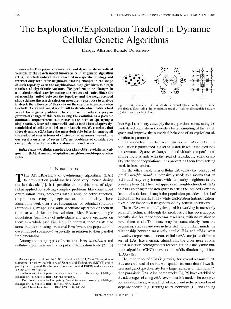
Fig. 8. Change in the ratio performed when conditions C and C ofAlgorithm 2 hold.

algorithm evolves slowly, i.e., when the convergence speed de-cays below a given threshold value . This is rep-resented by the condition of line 1 in Algorithm 2. If, on theother side, the search is proceeding too fast, diversity could belost quickly and there exists a risk of getting stuck in a local op-timum. In this second case, the population shape will be changedto a narrower grid and, thus, promote exploration and diversityin the forthcoming generations. The condition for detecting thissituation is expressed by line 3 in Algorithm 2. If neither nor

are true, the shape is not changed (line 6).As it can be seen, this is a general search pattern, and mul-

tiple criteria could be used to control whether the algo-rithm should explore or exploit the individuals for the nextgenerations.

The objective of these adaptive criteria is to maintain the di-versity and to pursue the global optimum during the execution.Notice that a change in the grid shape implies the relocation ofindividuals, which is a kind of migration since individuals indifferent areas become neighbors. Therefore, this change in thetopology is also an additional source for increasing the diversity,intrinsic to the adaptive criterion.

Whenever the criterion is fulfilled, the adaptive searchpattern performs a change in the grid shape. The functionChangeTo(square/narrow) in Algorithm 2 changes the grid tothe immediately next more square/narrow allowed shape. Thebounding cases are the square grid shape and the completelylinear (ring-like) shape, as shown in Fig. 8. When the currentgrid is square and the algorithm needs to change to the next“more square” one, or when the present grid shape is thenarrowest one and the algorithm needs to change to the next“narrower” one, the algorithm does not make any change in thepopulation shape at all. In the rest of cases, when the change ispossible, it is accomplished by computing a new position forevery individual whose general location is , as shown in(3). Of course, other changes could have been used, but, in ourquest for efficiency, the proposed one is considered to introducea negligible overhead.

Once we have fixed the basic adaptive pattern and grid shapemodification rules, we now proceed to explain the criteria usedto determine when the population is going “too” fast or “too”slow. We propose in this paper three different criteria for mea-suring the search speed. The measures are based on the averagefitness (criterion AF), the population entropy (criterion PH), oron a combination of the two (criterion ). Since thesecriteria check simple conditions over the average fitness and thepopulation entropy (calculated in every run in the populationstatistics computation step), we can say that they are inexpen-sive to measure, and they are indicative of the search states atthe same time too. The complexity for calculating the average

fitness is , while in the case of the population entropy it isbeing the size of the population and the length of

the chromosomes. The details on their internals are as follows.

• AF: This criterion is based on the average fitness of thepopulation. Hence, our measure of the convergence speedis based in terms of the diversity of phenotypes. We define

as the difference between the average fitness valuesin generation and . The algorithmwill change the ratio value to the immediately larger one(keeping constant the population size) if the difference

between two contiguous generations ( and )decreases at least in a factor of

(condition of Algorithm 2). On the contrary,the ratio will be changed to its closer smaller value if thatdifference increases in a factor greater than

(condition ). Formally, wedefine and as follows:

• PH: We now propose to measure the convergence speed interms of the genotypic diversity. The population entropy isthe metric used for this purpose. We calculate this entropy

as the average value of the entropy of each genein the population. Hence, this criterion is similar to AFexcept for that it uses the change in the population entropybetween two generations instead ofthe average fitness variation. Consequently, conditionsand are expressed as

• : This is the third and last proposed criterion tocreate an adaptive cGA. It considers both the populationentropy and the average fitness acceleration by combiningthe two previous criteria (AF and PH). Thus, it relays onthe phenotype and genotype diversity in order to obtainthe best exploration/exploitation tradeoff. This is a morerestrictive criterion with respect to the two previous ones,since although genetic diversity usually implies pheno-typic diversity, the reciprocal is not always true. Condi-tion in this case is the result of the logic operationof conditions of the two preceding criteria. In the sameway, will be the operation of conditions of AFand PH

Moreover, for each adaptive criterion (AF, PH, and ),we can begin the execution by using: 1) the square grid shape;2) the narrowest one; or 3) the one having a medium ratio value(rectangular). In our terminology, we will specify the initial gridshape by adding at the beginning of the criterion name a , or


Fig. 9. Basic deceptive bipolar function (s ) for MMDP.

for executions that begins at the square, narrowest, or rectan-gular ratio grid shapes, respectively. For example, the algorithmwhich uses criterion AF beginning at the narrowest shape willbe denoted as AF.

In short, we have proposed in this section three different adap-tive criteria. The first one, AF, is based on the phenotypic diver-sity, while the second one, PH, is based on genotypic diversity.Finally, is a combined criterion accounting for diver-sity at these two levels.

V. TEST PROBLEMS

In this section, we present the set of problems chosen forthis study. The benchmark is representative because it containsmany different interesting features in optimization, such asepistasis, multimodality, deceptiveness, use of constraints,parameter identification, and problem generators. These are im-portant ingredients in any work trying to evaluate algorithmicapproaches with the objective of getting reliable results, asstated by Whitley et al. in [29].

Initially, we will experiment with the reduced set of prob-lems studied in [17], which includes the massively multimodaldeceptive problem (MMDP), the frequency modulation sounds(FMS), and the multimodal problem generator P-PEAKS;next, we will extend this basic three-problem benchmark withCOUNTSAT (an instance of MAXSAT), error correcting codedesign (ECC), maximum cut of a graph (MAXCUT), and theminimum tardy task problem (MTTP). The election of thisset of problems is justified by both their difficulty and theirapplication domains (combinatorial optimization, continuousoptimization, telecommunications, scheduling, etc.). This guar-antees a high level of confidence in the results, although theevaluation of conclusions will result more laborious than witha small test suite.

The problems selected for this benchmark are explained inSections V-A–V-G. We include the explanations in this paper tomake it self-contained and to avoid the typical small lacks thatcould preclude other researchers from reproducing the results.

A. Massively Multimodal Deceptive Problem (MMDP)

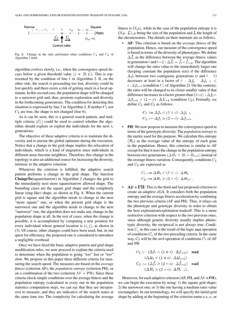
The MMDP is a problem that has been specifically designedto be difficult for an EA [30]. It is made up of deceptive sub-problems of 6 bits each one, whose value depends on thenumber of ones (unitation) a binary string has (see Fig. 9). It iseasy to see (graphic of Fig. 9) that these subfunctions have twoglobal maxima and a deceptive attractor in the middle point.

In MMDP, each subproblem contributes to the fitness valueaccording to its unitation (Fig. 9). The global optimum has a

value of and it is attained when every subproblem is composedof zero or six ones. The number of local optima is quite large

, while there are only global solutions. Therefore, thedegree of multimodality is regulated by the parameter. We usehere a considerably large instance of subproblems. Theinstance we try to maximize for solving the problem is shownin (4), and its maximum value is 40

fitness (4)

B. Frequency Modulation Sounds (FMS)

The FMS problem [31] is defined as determining the six real-parameters of the frequency mod-ulated sound model given in (5) for approximating it to thesound wave given in (6) (where ). The parametersare defined in the range , and we encode each pa-rameter into a 32 bit substring in the individual

(5)

(6)

The goal is to minimize the sum of square errors given by (7).This problem is a highly complex multimodal function havingstrong epistasis, with optimum value 0.0. Due to the high diffi-culty of solving this problem with high accuracy without ap-plying local search or specific operators for continuous opti-mization (like gradual GAs [19]), we stop the algorithm whenthe error falls below 10 . Hence, our objective for this problemwill be to minimize (7)

(7)

C. Multimodal Problem Generator (P-PEAKS)

The P-PEAKS problem [32] is a multimodal problem gen-erator. A problem generator is an easily parameterizable taskwhich has a tunable degree of difficulty. Also, using a problemgenerator removes the opportunity to hand-tune algorithms toa particular problem, therefore allowing a larger fairness whencomparing algorithms. With a problem generator, we evaluateour algorithms on a high number of random problem instances,since a different instance is solved each time the algorithm runs,then the predictive power of the results for the problem class asa whole is increased.

The idea of P-PEAKS is to generate random -bit stringsthat represent the location of peaks in the search space. Thefitness value of a string is the number of bits the string has incommon with the nearest peak in that space, divided by [asshown in (8)]. As stated in [32], “ Problems with a small/largenumber of peaks are weakly/strongly epistatic .” In this paper,we have used an instance of peaks of length


Fig. 10. COUNTSAT function with n = 20 variables.

bits each, which represents a medium/high difficulty level[17]. The maximum fitness value for this problem is 1.0

Hamming Peak

(8)

D. COUNTSAT Problem

The COUNTSAT problem [33] is an instance of MAXSAT.Let us consider the following clauses [34]:

• ;• .In COUNTSAT, the solution value is the number of clauses

(among those specified above) that are satisfied by a -bit inputstring. It is easy to check that the optimum value is that havingall the variables set to 1 . In this work, an instance of

variables has been used, with optimum value of 6860(9)

(9)

The COUNTSAT function is extracted from MAXSAT withthe objective of being very difficult to solve with GAs [33].Every uniformly generated random input will have approxi-mately ones. Then, local changes decreasing the number ofones will lead to better inputs, while local changes increasingthe number of ones decrease the fitness (Fig. 10). Hence, wemight expect that EAs quickly find the all-zero string and havedifficulties to find the all-one string.

E. Error Correcting Code Design Problem (ECC)

The ECC problem was presented in [35]. We will consider athree-tuple , where is the length of each codeword(number of bits), is the number of codewords, and is theminimum Hamming distance between any pair of codewords.Our objective will be to find a code which has a value foras large as possible (reflecting greater tolerance to noise and

errors), given previously fixed values for and . The problemwe have studied is basically the same presented in [35]. Thefitness function to be maximized is

(10)

where represents the Hamming distance between codewordsand in the code (made up of codewords, each of length). We consider in the present paper an instance where

and . The search space is of size , which isapproximately 10 . The optimum solution for and

has a fitness value of 0.0674 [36].

F. Maximum Cut of a Graph (MAXCUT)

The MAXCUT problem looks for a partition of the set of ver-tices of a weighted graph into two disjoint sub-sets and so that the sum of the weights of the edges withone endpoint in and the other one in is maximized. Forencoding the problem, we use a binary stringof length , where each digit corresponds to a vertex. If a digitis 1, then the corresponding vertex is in set ; if it is 0, then thecorresponding vertex is in set . The function to be maximized[37] is

(11)

Note that contributes to the sum only if nodes and arein different partitions. We have considered three different graphexamples in this study. Two of them are randomly generatedgraphs of moderate sizes: a sparse one “cut20.01” and a denseone “cut20.09,” both of them are made up of 20 vertices. Theother instance is a scalable weighted graph of 100 vertices. Theglobally optimal solutions for these instances are 10.119 812 for“cut20.01,” 56.740 064 in the case of “cut20.09,” and 1077 for“cut100” [37].

G. Minimum Tardy Task Problem (MTTP)

MTTP [38] is a task-scheduling problem, wherein each taskfrom the set of tasks has a length (the timeit takes for its execution), a deadline (before which a taskmust be scheduled, and its execution completed), and a weight

. The weight is a penalty that has to be added to the objectivefunction in the event that the task remains unscheduled. Thelengths, weights and deadlines of tasks are all positive integers.Scheduling the tasks of a subset of is to find the starting timeof each task in , such as at most one task at time is performedand such that each task finishes before its deadline.

We characterize a one-to-one scheduling function definedon a subset of tasks , so that for all tasks

has the following properties.

1) A task cannot be scheduled before any previous one hasfinished: .

2) Every task finishes before its deadline: .


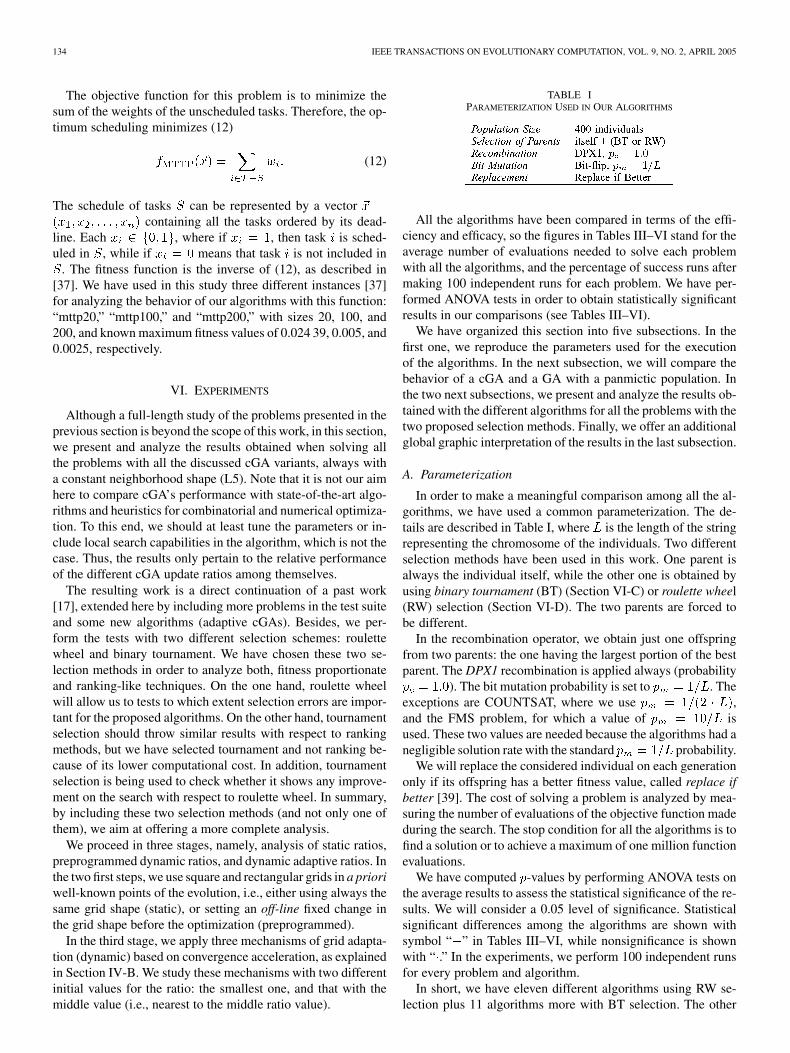
The objective function for this problem is to minimize thesum of the weights of the unscheduled tasks. Therefore, the op-timum scheduling minimizes (12)

(12)

The schedule of tasks can be represented by a vectorcontaining all the tasks ordered by its dead-

line. Each , where if , then task is sched-uled in , while if means that task is not included in

. The fitness function is the inverse of (12), as described in[37]. We have used in this study three different instances [37]for analyzing the behavior of our algorithms with this function:“mttp20,” “mttp100,” and “mttp200,” with sizes 20, 100, and200, and known maximum fitness values of 0.024 39, 0.005, and0.0025, respectively.

VI. EXPERIMENTS

Although a full-length study of the problems presented in theprevious section is beyond the scope of this work, in this section,we present and analyze the results obtained when solving allthe problems with all the discussed cGA variants, always witha constant neighborhood shape (L5). Note that it is not our aimhere to compare cGA’s performance with state-of-the-art algo-rithms and heuristics for combinatorial and numerical optimiza-tion. To this end, we should at least tune the parameters or in-clude local search capabilities in the algorithm, which is not thecase. Thus, the results only pertain to the relative performanceof the different cGA update ratios among themselves.

The resulting work is a direct continuation of a past work[17], extended here by including more problems in the test suiteand some new algorithms (adaptive cGAs). Besides, we per-form the tests with two different selection schemes: roulettewheel and binary tournament. We have chosen these two se-lection methods in order to analyze both, fitness proportionateand ranking-like techniques. On the one hand, roulette wheelwill allow us to tests to which extent selection errors are impor-tant for the proposed algorithms. On the other hand, tournamentselection should throw similar results with respect to rankingmethods, but we have selected tournament and not ranking be-cause of its lower computational cost. In addition, tournamentselection is being used to check whether it shows any improve-ment on the search with respect to roulette wheel. In summary,by including these two selection methods (and not only one ofthem), we aim at offering a more complete analysis.

We proceed in three stages, namely, analysis of static ratios,preprogrammed dynamic ratios, and dynamic adaptive ratios. Inthe two first steps, we use square and rectangular grids in a prioriwell-known points of the evolution, i.e., either using always thesame grid shape (static), or setting an off-line fixed change inthe grid shape before the optimization (preprogrammed).

In the third stage, we apply three mechanisms of grid adapta-tion (dynamic) based on convergence acceleration, as explainedin Section IV-B. We study these mechanisms with two differentinitial values for the ratio: the smallest one, and that with themiddle value (i.e., nearest to the middle ratio value).

TABLE IPARAMETERIZATION USED IN OUR ALGORITHMS

All the algorithms have been compared in terms of the effi-ciency and efficacy, so the figures in Tables III–VI stand for theaverage number of evaluations needed to solve each problemwith all the algorithms, and the percentage of success runs aftermaking 100 independent runs for each problem. We have per-formed ANOVA tests in order to obtain statistically significantresults in our comparisons (see Tables III–VI).

We have organized this section into five subsections. In thefirst one, we reproduce the parameters used for the executionof the algorithms. In the next subsection, we will compare thebehavior of a cGA and a GA with a panmictic population. Inthe two next subsections, we present and analyze the results ob-tained with the different algorithms for all the problems with thetwo proposed selection methods. Finally, we offer an additionalglobal graphic interpretation of the results in the last subsection.

A. Parameterization

In order to make a meaningful comparison among all the al-gorithms, we have used a common parameterization. The de-tails are described in Table I, where is the length of the stringrepresenting the chromosome of the individuals. Two differentselection methods have been used in this work. One parent isalways the individual itself, while the other one is obtained byusing binary tournament (BT) (Section VI-C) or roulette wheel(RW) selection (Section VI-D). The two parents are forced tobe different.

In the recombination operator, we obtain just one offspringfrom two parents: the one having the largest portion of the bestparent. The DPX1 recombination is applied always (probability

). The bit mutation probability is set to . Theexceptions are COUNTSAT, where we use ,and the FMS problem, for which a value of isused. These two values are needed because the algorithms had anegligible solution rate with the standard probability.

We will replace the considered individual on each generationonly if its offspring has a better fitness value, called replace ifbetter [39]. The cost of solving a problem is analyzed by mea-suring the number of evaluations of the objective function madeduring the search. The stop condition for all the algorithms is tofind a solution or to achieve a maximum of one million functionevaluations.

We have computed -values by performing ANOVA tests onthe average results to assess the statistical significance of the re-sults. We will consider a 0.05 level of significance. Statisticalsignificant differences among the algorithms are shown withsymbol “ ” in Tables III–VI, while nonsignificance is shownwith “ .” In the experiments, we perform 100 independent runsfor every problem and algorithm.

In short, we have eleven different algorithms using RW se-lection plus 11 algorithms more with BT selection. The other


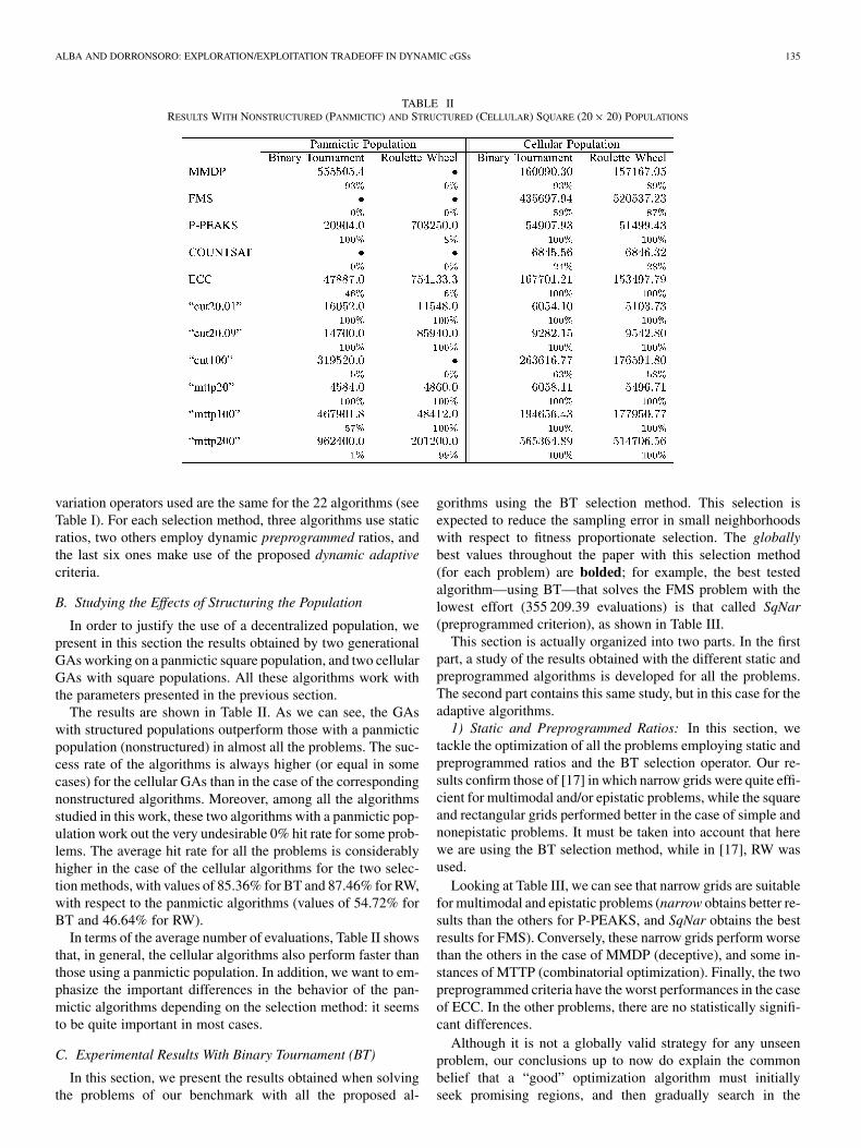
TABLE IIRESULTS WITH NONSTRUCTURED (PANMICTIC) AND STRUCTURED (CELLULAR) SQUARE (20� 20) POPULATIONS

variation operators used are the same for the 22 algorithms (seeTable I). For each selection method, three algorithms use staticratios, two others employ dynamic preprogrammed ratios, andthe last six ones make use of the proposed dynamic adaptivecriteria.

B. Studying the Effects of Structuring the Population

In order to justify the use of a decentralized population, wepresent in this section the results obtained by two generationalGAs working on a panmictic square population, and two cellularGAs with square populations. All these algorithms work withthe parameters presented in the previous section.

The results are shown in Table II. As we can see, the GAswith structured populations outperform those with a panmicticpopulation (nonstructured) in almost all the problems. The suc-cess rate of the algorithms is always higher (or equal in somecases) for the cellular GAs than in the case of the correspondingnonstructured algorithms. Moreover, among all the algorithmsstudied in this work, these two algorithms with a panmictic pop-ulation work out the very undesirable 0% hit rate for some prob-lems. The average hit rate for all the problems is considerablyhigher in the case of the cellular algorithms for the two selec-tion methods, with values of 85.36% for BT and 87.46% for RW,with respect to the panmictic algorithms (values of 54.72% forBT and 46.64% for RW).

In terms of the average number of evaluations, Table II showsthat, in general, the cellular algorithms also perform faster thanthose using a panmictic population. In addition, we want to em-phasize the important differences in the behavior of the pan-mictic algorithms depending on the selection method: it seemsto be quite important in most cases.

C. Experimental Results With Binary Tournament (BT)

In this section, we present the results obtained when solvingthe problems of our benchmark with all the proposed al-

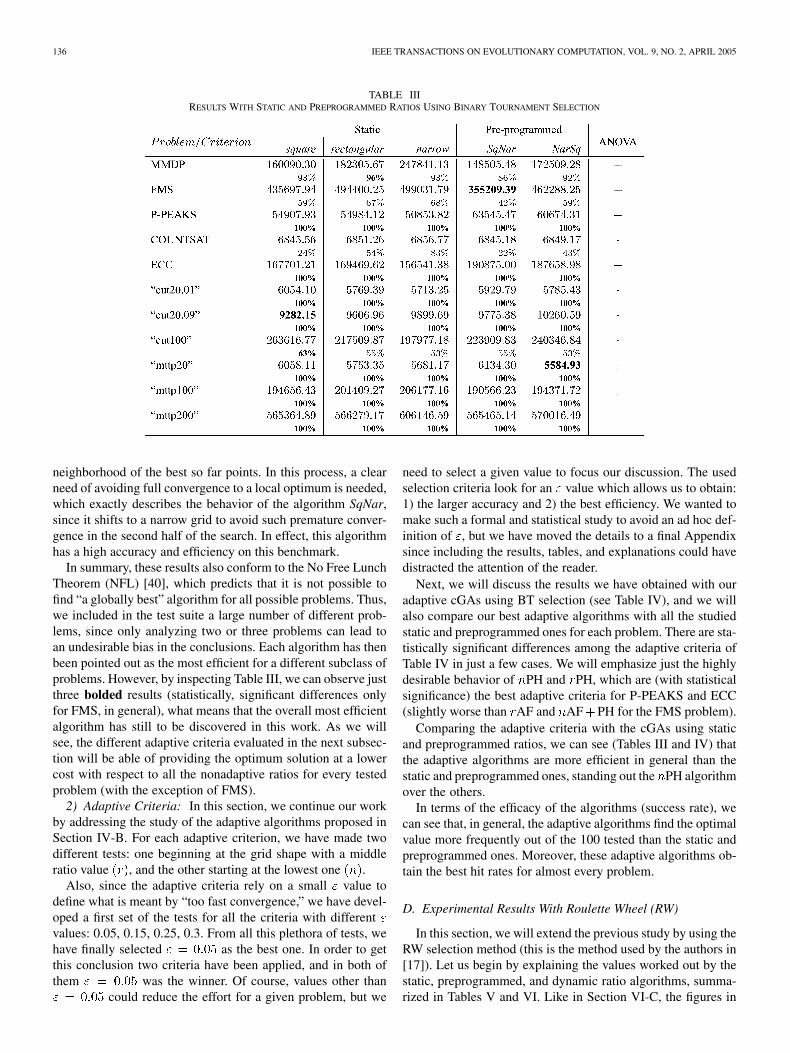
gorithms using the BT selection method. This selection isexpected to reduce the sampling error in small neighborhoodswith respect to fitness proportionate selection. The globallybest values throughout the paper with this selection method(for each problem) are bolded; for example, the best testedalgorithm—using BT—that solves the FMS problem with thelowest effort (355 209.39 evaluations) is that called SqNar(preprogrammed criterion), as shown in Table III.

This section is actually organized into two parts. In the firstpart, a study of the results obtained with the different static andpreprogrammed algorithms is developed for all the problems.The second part contains this same study, but in this case for theadaptive algorithms.

1) Static and Preprogrammed Ratios: In this section, wetackle the optimization of all the problems employing static andpreprogrammed ratios and the BT selection operator. Our re-sults confirm those of [17] in which narrow grids were quite effi-cient for multimodal and/or epistatic problems, while the squareand rectangular grids performed better in the case of simple andnonepistatic problems. It must be taken into account that herewe are using the BT selection method, while in [17], RW wasused.

Looking at Table III, we can see that narrow grids are suitablefor multimodal and epistatic problems (narrow obtains better re-sults than the others for P-PEAKS, and SqNar obtains the bestresults for FMS). Conversely, these narrow grids perform worsethan the others in the case of MMDP (deceptive), and some in-stances of MTTP (combinatorial optimization). Finally, the twopreprogrammed criteria have the worst performances in the caseof ECC. In the other problems, there are no statistically signifi-cant differences.

Although it is not a globally valid strategy for any unseenproblem, our conclusions up to now do explain the commonbelief that a “good” optimization algorithm must initiallyseek promising regions, and then gradually search in the


TABLE IIIRESULTS WITH STATIC AND PREPROGRAMMED RATIOS USING BINARY TOURNAMENT SELECTION

neighborhood of the best so far points. In this process, a clearneed of avoiding full convergence to a local optimum is needed,which exactly describes the behavior of the algorithm SqNar,since it shifts to a narrow grid to avoid such premature conver-gence in the second half of the search. In effect, this algorithmhas a high accuracy and efficiency on this benchmark.

In summary, these results also conform to the No Free LunchTheorem (NFL) [40], which predicts that it is not possible tofind “a globally best” algorithm for all possible problems. Thus,we included in the test suite a large number of different prob-lems, since only analyzing two or three problems can lead toan undesirable bias in the conclusions. Each algorithm has thenbeen pointed out as the most efficient for a different subclass ofproblems. However, by inspecting Table III, we can observe justthree bolded results (statistically, significant differences onlyfor FMS, in general), what means that the overall most efficientalgorithm has still to be discovered in this work. As we willsee, the different adaptive criteria evaluated in the next subsec-tion will be able of providing the optimum solution at a lowercost with respect to all the nonadaptive ratios for every testedproblem (with the exception of FMS).

2) Adaptive Criteria: In this section, we continue our workby addressing the study of the adaptive algorithms proposed inSection IV-B. For each adaptive criterion, we have made twodifferent tests: one beginning at the grid shape with a middleratio value , and the other starting at the lowest one .

Also, since the adaptive criteria rely on a small value todefine what is meant by “too fast convergence,” we have devel-oped a first set of the tests for all the criteria with differentvalues: 0.05, 0.15, 0.25, 0.3. From all this plethora of tests, wehave finally selected as the best one. In order to getthis conclusion two criteria have been applied, and in both ofthem was the winner. Of course, values other than

could reduce the effort for a given problem, but we

need to select a given value to focus our discussion. The usedselection criteria look for an value which allows us to obtain:1) the larger accuracy and 2) the best efficiency. We wanted tomake such a formal and statistical study to avoid an ad hoc def-inition of , but we have moved the details to a final Appendixsince including the results, tables, and explanations could havedistracted the attention of the reader.

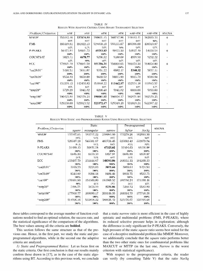
Next, we will discuss the results we have obtained with ouradaptive cGAs using BT selection (see Table IV), and we willalso compare our best adaptive algorithms with all the studiedstatic and preprogrammed ones for each problem. There are sta-tistically significant differences among the adaptive criteria ofTable IV in just a few cases. We will emphasize just the highlydesirable behavior of PH and PH, which are (with statisticalsignificance) the best adaptive criteria for P-PEAKS and ECC(slightly worse than AF and AF PH for the FMS problem).

Comparing the adaptive criteria with the cGAs using staticand preprogrammed ratios, we can see (Tables III and IV) thatthe adaptive algorithms are more efficient in general than thestatic and preprogrammed ones, standing out the PH algorithmover the others.

In terms of the efficacy of the algorithms (success rate), wecan see that, in general, the adaptive algorithms find the optimalvalue more frequently out of the 100 tested than the static andpreprogrammed ones. Moreover, these adaptive algorithms ob-tain the best hit rates for almost every problem.

D. Experimental Results With Roulette Wheel (RW)

In this section, we will extend the previous study by using theRW selection method (this is the method used by the authors in[17]). Let us begin by explaining the values worked out by thestatic, preprogrammed, and dynamic ratio algorithms, summa-rized in Tables V and VI. Like in Section VI-C, the figures in


TABLE IVRESULTS WITH ADAPTIVE CRITERIA USING BINARY TOURNAMENT SELECTION

TABLE VRESULTS WITH STATIC AND PREPROGRAMMED RATIOS USING ROULETTE WHEEL SELECTION

these tables correspond to the average number of function eval-uations needed to find an optimal solution, the success rate, andthe statistical significance of the comparison of the algorithms.The best values among all the criteria are bolded.

This section follows the same structure as that of the pre-vious one. Hence, in the first part, we study the static and pre-programmed algorithms, while in the second one the adaptivecriteria are analyzed.

1) Static and Preprogrammed Ratios: Let us focus first onthe static criteria. Our first conclusion is that our results mainlyconfirm those drawn in [17], as in the case of the static algo-rithms using BT. According to this previous work, we conclude

that a static narrow ratio is more efficient in the case of highlyepistatic and multimodal problems (FMS, P-PEAKS), whereits reduced selective pressure helps in exploration; althoughthe difference is only significant for P-PEAKS. Conversely, thehigh pressure of the static square ratio seems best suited for thecase of a deceptive multimodal problem like MMDP. Moreover,we additionally conclude that the square ratio performs betterthan the two other static ones for combinatorial problems likeMAXCUT or MTTP (in the last one, Narrow is the worstcriterion with statistical significance).

With respect to the preprogrammed criteria, the readercan verify (by consulting Table V) that the ratio NarSq


TABLE VIRESULTS WITH ADAPTIVE CRITERIA USING ROULETTE WHEEL SELECTION

TABLE VIICOMPARING THE BEST ADAPTIVE CRITERIA VERSUS NONADAPTIVE RATIOS USING BINARY TOURNAMENT AND ROULETTE WHEEL (BT, RW)

(exploration-to-exploitation) does not improve the best resultsobtained with respect to the rest of static and preprogrammedstudied criteria in any case. Besides, the other proposed pre-programmed ratio SqNar (which represents a change for largerdiversity in the second phase of the algorithm) outperforms theefficiency of the other criteria of Table V only for the instance“mttp100,” although there is no statistical significance. Thetwo preprogrammed criteria are worse than all the static oneswith statistical significance in the cases of ECC and P-PEAKSproblems.

2) Adaptive Criteria: As we did in Section VI-C2, we willstudy the behavior of our adaptive algorithms with the RW se-lection method, and compare them with the static and prepro-grammed ones. In Table VI, we show the results obtained withthe six adaptive criteria. The first conclusion we can draw fromthat table is that, as in the case of Section VI-C2, the behaviorof the algorithms is globally improved by making them adaptive(notice the large number of boldfaced results, i.e., most efficientalgorithms).

Moreover, the most effective algorithm for every problem isalways an adaptive one. The reader can verify it in Tables Vand VI, since the highest hit rates for every problem are ob-

tained by the adaptive algorithms. Hence, we can conclude that,in general, the adaptive algorithms (either using binary tourna-ment or roulette wheel) outperform the other studied ones in thetwo checked features: efficiency and efficacy.

In Table VII, we compare, for every problem, our best adap-tive algorithm with the static and preprogrammed ones. Thistable accounts for algorithms using both BT and RW selec-tion methods. Symbol “ ” means that the adaptive algorithm isbetter with statistical significance than the compared nonadap-tive one, while “ ” stands for nonsignificant differences. We cansee that, for the two selection methods, there is not any staticor preprogrammed algorithm better than the best adaptive onefor every problem. Hence, the bolded values in Tables III andV corresponding to a best nonadaptive algorithm are undistin-guishable of the adaptive ones. For all the problems, the existingstatistically significant differences favors the adaptive criteriaagainst the static and preprogrammed ones.

E. Additional Discussion

If we look among all the adaptive criteria, we conclude (asexpected from the theory) that there is no adaptive criterionthat significatively outperforms the rest for all the test suite,


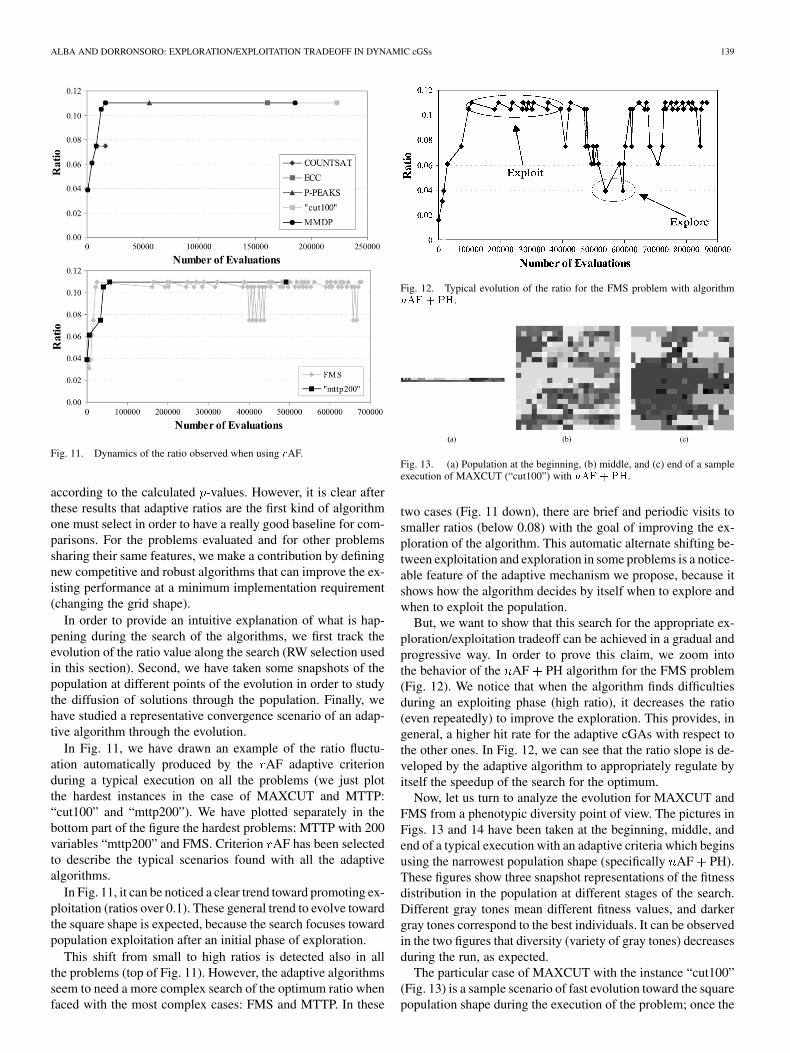
Fig. 11. Dynamics of the ratio observed when using rAF.

according to the calculated -values. However, it is clear afterthese results that adaptive ratios are the first kind of algorithmone must select in order to have a really good baseline for com-parisons. For the problems evaluated and for other problemssharing their same features, we make a contribution by definingnew competitive and robust algorithms that can improve the ex-isting performance at a minimum implementation requirement(changing the grid shape).

In order to provide an intuitive explanation of what is hap-pening during the search of the algorithms, we first track theevolution of the ratio value along the search (RW selection usedin this section). Second, we have taken some snapshots of thepopulation at different points of the evolution in order to studythe diffusion of solutions through the population. Finally, wehave studied a representative convergence scenario of an adap-tive algorithm through the evolution.

In Fig. 11, we have drawn an example of the ratio fluctu-ation automatically produced by the AF adaptive criterionduring a typical execution on all the problems (we just plotthe hardest instances in the case of MAXCUT and MTTP:“cut100” and “mttp200”). We have plotted separately in thebottom part of the figure the hardest problems: MTTP with 200variables “mttp200” and FMS. Criterion AF has been selectedto describe the typical scenarios found with all the adaptivealgorithms.

In Fig. 11, it can be noticed a clear trend toward promoting ex-ploitation (ratios over 0.1). These general trend to evolve towardthe square shape is expected, because the search focuses towardpopulation exploitation after an initial phase of exploration.

This shift from small to high ratios is detected also in allthe problems (top of Fig. 11). However, the adaptive algorithmsseem to need a more complex search of the optimum ratio whenfaced with the most complex cases: FMS and MTTP. In these

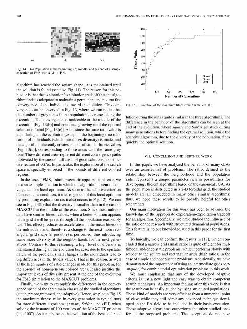
Fig. 12. Typical evolution of the ratio for the FMS problem with algorithmnAF + PH.

Fig. 13. (a) Population at the beginning, (b) middle, and (c) end of a sampleexecution of MAXCUT (“cut100”) with nAF + PH.

two cases (Fig. 11 down), there are brief and periodic visits tosmaller ratios (below 0.08) with the goal of improving the ex-ploration of the algorithm. This automatic alternate shifting be-tween exploitation and exploration in some problems is a notice-able feature of the adaptive mechanism we propose, because itshows how the algorithm decides by itself when to explore andwhen to exploit the population.

But, we want to show that this search for the appropriate ex-ploration/exploitation tradeoff can be achieved in a gradual andprogressive way. In order to prove this claim, we zoom intothe behavior of the AF PH algorithm for the FMS problem(Fig. 12). We notice that when the algorithm finds difficultiesduring an exploiting phase (high ratio), it decreases the ratio(even repeatedly) to improve the exploration. This provides, ingeneral, a higher hit rate for the adaptive cGAs with respect tothe other ones. In Fig. 12, we can see that the ratio slope is de-veloped by the adaptive algorithm to appropriately regulate byitself the speedup of the search for the optimum.

Now, let us turn to analyze the evolution for MAXCUT andFMS from a phenotypic diversity point of view. The pictures inFigs. 13 and 14 have been taken at the beginning, middle, andend of a typical execution with an adaptive criteria which beginsusing the narrowest population shape (specifically AF PH).These figures show three snapshot representations of the fitnessdistribution in the population at different stages of the search.Different gray tones mean different fitness values, and darkergray tones correspond to the best individuals. It can be observedin the two figures that diversity (variety of gray tones) decreasesduring the run, as expected.

The particular case of MAXCUT with the instance “cut100”(Fig. 13) is a sample scenario of fast evolution toward the squarepopulation shape during the execution of the problem; once the


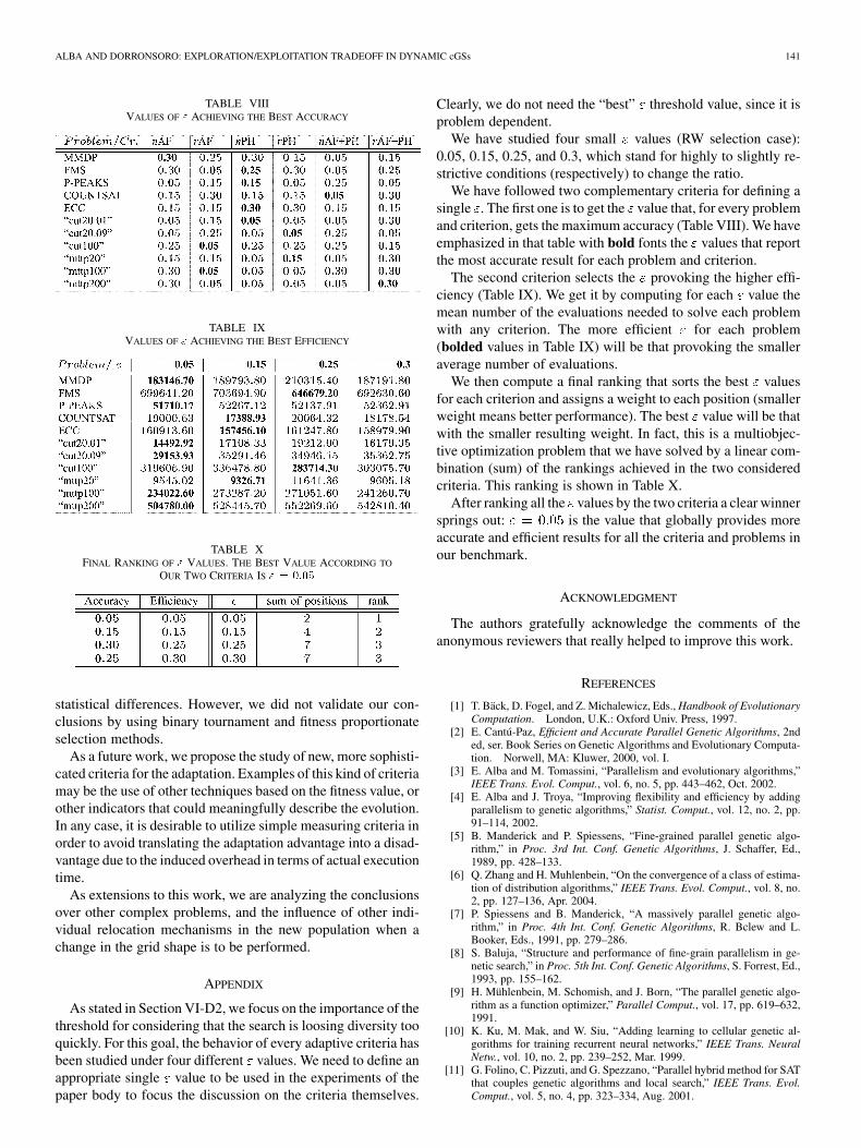
Fig. 14. (a) Population at the beginning, (b) middle, and (c) end of a sampleexecution of FMS with nAF + PH.

algorithm has reached the square shape, it is maintained untilthe solution is found (see also Fig. 11). The reason for this be-havior is that the exploration/exploitation tradeoff that the algo-rithm finds is adequate to maintain a permanent and not too fastconvergence of the individuals toward the solution. This con-vergence can be observed in Fig. 13, where we can notice thatthe number of grey tones in the population decreases along theexecution. The convergence is noticeable at the middle of theexecution [Fig. 13(b)] and continues growing until the optimalsolution is found [Fig. 13(c)]. Also, since the same ratio value iskept during all the evolution (except at the beginning), no relo-cation of individuals (which introduces diversity) is made, andthe algorithm inherently creates islands of similar fitness values[Fig. 13(c)], corresponding to those areas with the same graytone. These different areas represent different convergence pathsmotivated by the smooth diffusion of good solutions, a distinc-tive feature of cGAs. In particular, the exploration of the searchspace is specially enforced in the bounds of different coloredregions.

In the case of FMS, a similar scenario appears; in this case, weplot an example situation in which the algorithm is near to con-vergence to a local optimum. As soon as the adaptive criteriondetects such a condition, it tries to get out of this local optimumby promoting exploration (as it also occurs in Fig. 12). We cansee in Fig. 14(b) that the diversity is smaller than in the case ofMAXCUT in the middle of the execution. Since most individ-uals have similar fitness values, when a better solution appearsin the grid it will be spread through all the population reasonablyfast. This effect produces an acceleration in the mean fitness ofthe individuals and, therefore, a change to the next more rect-angular grid shape (if possible) is performed, thus introducingsome more diversity at the neighborhoods for the next gener-ations. Contrary to this reasoning, a high level of diversity ismaintained during all the evolution because, due to the epistaticnature of the problem, small changes in the individuals lead tobig differences in the fitness values. That is the reason, as wellas the high number of ratio changes made for this problem, forthe absence of homogeneous colored areas. It also justifies theimportant levels of diversity present at the end of the evolutionfor FMS (in relation to the MAXCUT problem).

Finally, we want to exemplify the differences in the conver-gence speed of the three main classes of the studied algorithms(static, preprogrammed, and adaptive). Hence, we plot in Fig. 15the maximum fitness value in every generation in typical runsfor three different algorithms (square, SqNar, and PH) whensolving the instance of 100 vertices of the MAXCUT problem(“cut100”). As it can be seen, the evolution of the best so far so-

Fig. 15. Evolution of the maximum fitness found with “cut100.”

lution during the run is quite similar in the three algorithms. Thedifference in the behavior of the algorithms can be seen at theend of the evolution, where square and SqNar get stuck duringmany generations before finding the optimal solution, while theadaptive algorithm, due to the diversity of the population, findsquickly the optimal solution.

VII. CONCLUSION AND FURTHER WORK

In this paper, we have analyzed the behavior of many cEAsover an assorted set of problems. The ratio, defined as therelationship between the neighborhood and the populationradii, represents a unique parameter rich in possibilities fordeveloping efficient algorithms based on the canonical cGA. Asthe population is distributed in a 2-D toroidal grid, the studiedmodels are all embedded in many other similar algorithms;thus, we hope these results to be broadly helpful for otherresearchers.

Our main motivation for this work has been to advance theknowledge of the appropriate exploration/exploitation tradeofffor an algorithm. Specifically, we have studied the influence ofthe ratio on the research with structured dynamical populations.This feature is, to our knowledge, used in this paper for the firsttime.

Technically, we can confirm the results in [17], which con-cluded that a narrow grid (small ratio) is quite efficient for mul-timodal and/or epistatic problems, while it performs slowly withrespect to the square and rectangular grids (high ratios) in thecase of simple and nonepistatic problems. Additionally, we havedemonstrated the importance of using an intermediate grid (rect-angular) for combinatorial optimization problems in this work.

We must emphasize that any of the developed adaptivecriteria is just a new light and easy way to obtain competentsearch techniques. An important feeling after this work is thatthe search can be easily guided by using structured populations.These kind of models are very efficient from a numerical pointof view, while they still admit any advanced technique devel-oped in the EA field to be included in their basic execution.These adaptive algorithms outperform the other studied onesfor all the proposed problems. The exceptions do not have


TABLE VIIIVALUES OF " ACHIEVING THE BEST ACCURACY

TABLE IXVALUES OF " ACHIEVING THE BEST EFFICIENCY

TABLE XFINAL RANKING OF " VALUES. THE BEST VALUE ACCORDING TO

OUR TWO CRITERIA IS " = 0:05

statistical differences. However, we did not validate our con-clusions by using binary tournament and fitness proportionateselection methods.

As a future work, we propose the study of new, more sophisti-cated criteria for the adaptation. Examples of this kind of criteriamay be the use of other techniques based on the fitness value, orother indicators that could meaningfully describe the evolution.In any case, it is desirable to utilize simple measuring criteria inorder to avoid translating the adaptation advantage into a disad-vantage due to the induced overhead in terms of actual executiontime.

As extensions to this work, we are analyzing the conclusionsover other complex problems, and the influence of other indi-vidual relocation mechanisms in the new population when achange in the grid shape is to be performed.

APPENDIX

As stated in Section VI-D2, we focus on the importance of thethreshold for considering that the search is loosing diversity tooquickly. For this goal, the behavior of every adaptive criteria hasbeen studied under four different values. We need to define anappropriate single value to be used in the experiments of thepaper body to focus the discussion on the criteria themselves.

Clearly, we do not need the “best” threshold value, since it isproblem dependent.

We have studied four small values (RW selection case):0.05, 0.15, 0.25, and 0.3, which stand for highly to slightly re-strictive conditions (respectively) to change the ratio.

We have followed two complementary criteria for defining asingle . The first one is to get the value that, for every problemand criterion, gets the maximum accuracy (Table VIII). We haveemphasized in that table with bold fonts the values that reportthe most accurate result for each problem and criterion.

The second criterion selects the provoking the higher effi-ciency (Table IX). We get it by computing for each value themean number of the evaluations needed to solve each problemwith any criterion. The more efficient for each problem(bolded values in Table IX) will be that provoking the smalleraverage number of evaluations.

We then compute a final ranking that sorts the best valuesfor each criterion and assigns a weight to each position (smallerweight means better performance). The best value will be thatwith the smaller resulting weight. In fact, this is a multiobjec-tive optimization problem that we have solved by a linear com-bination (sum) of the rankings achieved in the two consideredcriteria. This ranking is shown in Table X.

After ranking all the values by the two criteria a clear winnersprings out: is the value that globally provides moreaccurate and efficient results for all the criteria and problems inour benchmark.

ACKNOWLEDGMENT

The authors gratefully acknowledge the comments of theanonymous reviewers that really helped to improve this work.

REFERENCES

[1] T. Bäck, D. Fogel, and Z. Michalewicz, Eds., Handbook of EvolutionaryComputation. London, U.K.: Oxford Univ. Press, 1997.

[2] E. Cantú-Paz, Efficient and Accurate Parallel Genetic Algorithms, 2nded, ser. Book Series on Genetic Algorithms and Evolutionary Computa-tion. Norwell, MA: Kluwer, 2000, vol. I.

[3] E. Alba and M. Tomassini, “Parallelism and evolutionary algorithms,”IEEE Trans. Evol. Comput., vol. 6, no. 5, pp. 443–462, Oct. 2002.

[4] E. Alba and J. Troya, “Improving flexibility and efficiency by addingparallelism to genetic algorithms,” Statist. Comput., vol. 12, no. 2, pp.91–114, 2002.

[5] B. Manderick and P. Spiessens, “Fine-grained parallel genetic algo-rithm,” in Proc. 3rd Int. Conf. Genetic Algorithms, J. Schaffer, Ed.,1989, pp. 428–133.

[6] Q. Zhang and H. Muhlenbein, “On the convergence of a class of estima-tion of distribution algorithms,” IEEE Trans. Evol. Comput., vol. 8, no.2, pp. 127–136, Apr. 2004.

[7] P. Spiessens and B. Manderick, “A massively parallel genetic algo-rithm,” in Proc. 4th Int. Conf. Genetic Algorithms, R. Bclew and L.Booker, Eds., 1991, pp. 279–286.

[8] S. Baluja, “Structure and performance of fine-grain parallelism in ge-netic search,” in Proc. 5th Int. Conf. Genetic Algorithms, S. Forrest, Ed.,1993, pp. 155–162.

[9] H. Mühlenbein, M. Schomish, and J. Born, “The parallel genetic algo-rithm as a function optimizer,” Parallel Comput., vol. 17, pp. 619–632,1991.

[10] K. Ku, M. Mak, and W. Siu, “Adding learning to cellular genetic al-gorithms for training recurrent neural networks,” IEEE Trans. NeuralNetw., vol. 10, no. 2, pp. 239–252, Mar. 1999.

[11] G. Folino, C. Pizzuti, and G. Spezzano, “Parallel hybrid method for SATthat couples genetic algorithms and local search,” IEEE Trans. Evol.Comput., vol. 5, no. 4, pp. 323–334, Aug. 2001.


[12] M. Tomassini, “The parallel genetic cellular automata: Application toglobal function optimization,” in Proc. Int. Conf. Artif. Neural Netw. Ge-netic Algorithms, R. Albrecht, C. Reeves, and N. Steele, Eds, 1993, pp.385–391.

[13] D. Whitley, “Cellular genetic algorithms,” in Proc. 5th Int. Conf. GeneticAlgorithms, S. Forrest, Ed., 1993, p. 658.

[14] V. Gordon and D. Whitley, “Serial and parallel genetic algorithms asfunction optimizers,” in Proc. 5th Int. Conf. Genetic Algorithms, S. For-rest, Ed., 1993, pp. 177–183.

[15] J. Sarma and K. De Jong, “An analysis of the effect of the neighborhoodsize and shape on local selection algorithms,” in Lecture Notes in Com-puter Science, H. Voigt, W. Ebeling, I. Rechenberg, and H. Schwefel,Eds. Berlin, Germany: Springer-Verlag, 1996, vol. 1141, Proc. Int.Conf. Parallel Prob. Solving from Nature IV, pp. 236–244.

[16] , “An analysis of local selection algorithms in a spatially structuredevolutionary algorithm,” in Proc. 7th Int. Conf. Genetic Algorithms, T.Bäck, Ed., 1997, pp. 181–186.

[17] E. Alba and J. Troya, “Cellular evolutionary algorithms: Evaluating theinfluence of ratio,” in Lecture Notes in Computer Science, vol. 1917,Proc. Int. Conf. Parallel Prob. Solving from Nature VI, M. Schoenauer,Ed.. Berlin, Germany, 2000, pp. 29–38.

[18] M. Giacobini, E. Alba, and M. Tomassini, “Selection intensity inasynchronous cellular evolutionary algorithms,” in Proc. Genetic Evol.Comput. Conf., 2003, pp. 955–966.

[19] F. Herrera and M. Lozano, “Gradual distributed real-coded genetic algo-rithms,” IEEE Trans. Evol. Comput., vol. 4, no. 1, pp. 43–62, Apr. 2000.

[20] P. Adamidis and V. Petridis, “Co-operating populations with differentevolution behaviors,” in Proc. 3rd IEEE Conf. Evol. Comput., 1996, pp.188–191.

[21] Handbook of Applied Optimization, Memetic Algorithms, P. Pardalosand M. Resende, Eds., Oxford Univ. Press, London, U.K., 2000. P.Moscato.

[22] Y. Ong and A. Keane, “Meta-Lamarckian teaming in memetic algo-rithms,” IEEE Trans. Evol. Comput., vol. 8, no. 2, pp. 99–110, Apr. 2004.

[23] R. Hinterding, Z. Michalewicz, and A. Eiben, “Adaptation in evolu-tionary computation: A survey,” in Proc. IEEE Conf. Evol. Comput.,IEEE World Congr. Comput. Intell., 1997, pp. 65–69.

[24] T. Bäck, “Introduction to the special issue: Self-adaptation,” Evol.Comput., vol. 9, no. 2, pp. iii–iv, 2001.

[25] P. Angeline, “Adaptive and self-adaptive evolutionary computations,”in Computational Intelligence: A Dynamic Systems Perspective, M.Palaniswami and Y. Attikiouzel, Eds. Piscataway, NJ: IEEE Press,1995, pp. 152–163.

[26] L. Davis, “Adapting operator probabilities in genetic algorithms,” inProc. 3rd Int. Conf. Genetic Algorithms, J. Schaffer, Ed., 1989, pp.61–69.

[27] J. Arabas, Z. Michalewicz, and J. Mulawka, “GAVaPS—A genetic algo-rithm with varying population size,” in Proc. IEEE Conf. Evol. Comput.,vol. 1, 1994, pp. 73–78.

[28] D. Schlierkamp-Voosen and H. Mühlenbein, “Adaption of populationsizes by competing subpopulations,” in Proc. IEEE Conf. Evol. Comput.,1996, pp. 330–335.

[29] D. Whitley, S. Rana, J. Dzubera, and K. Mathias, “Evaluating evolu-tionary algorithms,” Artif. Intell., vol. 85, pp. 245–276, 1997.

[30] D. Goldberg, K. Deb, and J. Horn, “Massively multimodaliry, deception,and genetic algorithms,” in Proc. Int. Conf. Parallel Prob. Solving fromNature II, R. Männer and B. Manderick, Eds., 1992, pp. 37–46.

[31] S. Tsutsui and Y. Fujimoto, “Forking genetic algorithm with blockingand shrinking modes,” in Proc. 5th Int. Conf. Genetic Algorithms, S.Forrest, Ed., 1993, pp. 206–213.

[32] K. De Jong, M. Potter, and W. Spears, “Using problem generators to ex-plore the effects of epistasis,” in Proc. 7th Int. Conf. Genetic Algorithms,T. Bäck, Ed., 1997, pp. 338–345.

[33] S. Droste, T. Jansen, and I. Wegener, “A natural and simple functionwhich is hard for all evolutionary algorithms,” in Proc. 3rd Asia-PacificConf. Simulated Evol. Learning, 2000, pp. 2704–2709.

[34] C. Papadimitriou, Computational Complexity. Reading, MA: Ad-dison-Wesley, 1994.

[35] F. MacWilliams and N. Sloane, The Theory of Error-CorrectingCodes. Amsterdam, The Netherlands: North-Holland, 1977.

[36] H. Chen, N. Flann, and D. Watson, “Parallel genetic simulated an-nealing: A massively parallel SIMD algorithm,” IEEE Trans. ParallelDistrib. Syst., vol. 9, no. 2, pp. 126–136, 1998.

[37] S. Khuri, T. Bäck, and J. Heitkötter, “An evolutionary approach tocombinatorial optimization problems,” in Proc. 22nd ACM Comput.Sci. Conf., 1994, pp. 66–73.

[38] D. Stinson, An Introduction to the Design and Analysis of Algorithms,2nd ed. Winnipeg, MB, Canada: The Charles Babbage ResearchCenter, 1985, 1987.

[39] J. Smith and F. Vavak, “Replacement strategies in steady state genetic al-gorithms: Static environments,” in Foundations of Genetic Algorithms V,W. Banzhaf and C. Reeves, Eds: Morgan Kaufmann, 1998, pp. 219–234.

[40] D. Wolpert and W. Macready, “No free lunch theorems for optimiza-tion,” IEEE Trans. Evol. Comput., vol. 1, no. 1, pp. 67–82, Apr. 1997.

Enrique Alba received the Ph.D. degree in designingand analyzing parallel and distributed genetic algo-rithms from the University of Málaga, Málaga, Spain,in 1999.

He is a Professor of Computer Science at the Uni-versity of Málaga. He has published many scientificpapers in international conferences and journals, aswell as he holds national and international awardsto his research results. His current research interestsinvolve the design and application of evolutionary al-gorithms, neural networks, and other bioinspired sys-

tems to real problems including telecommunications, combinatorial optimiza-tion, and bioinformatics. The main focus of all his work is on parallelism.

Bernabé Dorronsoro received the Engineeringdegree in computer science from the University ofMálaga, Málaga, Spain, in 2002. He is currentlyworking towards the Ph.D. degree in the design ofnew evolutionary algorithms, specifically on struc-tured algorithms, and their application to complexproblems in the domains of logistics, telecommuni-cations, and combinatorial optimization.

126 IEEE TRANSACTIONS ON EVOLUTIONARY ...atarazanas.sci.uma.es/docs/tesisuma/1661480x.pdf128 IEEE TRANSACTIONS ON EVOLUTIONARY COMPUTATION, VOL. 9, NO. 2, APRIL 2005 Fig. 2. Growth

Documents