IEEE TRANSACTIONS ON EVOLUTIONARY COMPUTATION, VOL. 14, NO. 1, FEBRUARY 2010 1 Analysis of Computational Time of Simple Estimation of Distribution Algorithms Tianshi Chen, Student Member, IEEE, Ke Tang, Member, IEEE, Guoliang Chen, and Xin Yao, Fellow, IEEE NOTE: This paper was part of the Special Issue on Evolutionary Algorithms Based on Probabilistic Models that should have appeared in the IEEE TRANSACTIONS ON EVOLUTIONARY COMPUTATION, Vol. 13, No. 6, December 2009. Abstract —Estimation of distribution algorithms (EDAs) are widely used in stochastic optimization. Impressive experimental results have been reported in the literature. However, little work has been done on analyzing the computation time of EDAs in relation to the problem size. It is still unclear how well EDAs (with a finite population size larger than two) will scale up when the dimension of the optimization problem (problem size) goes up. This paper studies the computational time complexity of a simple EDA, i.e., the univariate marginal distribution algorithm (UMDA), in order to gain more insight into EDAs complex- ity. First, we discuss how to measure the computational time complexity of EDAs. A classification of problem hardness based on our discussions is then given. Second, we prove a theorem related to problem hardness and the probability conditions of EDAs. Third, we propose a novel approach to analyzing the computational time complexity of UMDA using discrete dynamic systems and Chernoff bounds. Following this approach, we are able to derive a number of results on the first hitting time of UMDA on a well-known unimodal pseudo-boolean function, i.e., the LeadingOnes problem, and another problem derived from LeadingOnes, named BVLeadingOnes. Although both problems are unimodal, our analysis shows that LeadingOnes is easy for the UMDA, while BVLeadingOnes is hard for the UMDA. Finally, in order to address the key issue of what problem characteristics make a problem hard for UMDA, we discuss in depth the idea of “margins” (or relaxation). We prove theoretically that the UMDA with margins can solve the BVLeadingOnes problem efficiently. Index Terms—Computational time complexity, estimation of distribution algorithms, first hitting time, heuristic optimization, univariate marginal distribution algorithms. Manuscript received November 26, 2007; revised October 28, 2008, February 5, 2009, and May 10, 2009. Current version published January 29, 2010. This work was supported in part by the National Natural Science Foundation of China under Grants 60533020 and U0835002, the Fund for Foreign Scholars in the University Research and Teaching Programs (111 Project) in China under Grant B07033, and an Engineering and Physical Science Research Council Grant EP/C520696/1 in the U.K. T. Chen, K. Tang, and G. Chen are with the Nature Inspired Computation and Applications Laboratory, School of Computer Science and Technology, University of Science and Technology of China, Hefei, Anhui 230027, China (e-mail: [email protected]; [email protected]; [email protected]). X. Yao is with the Nature Inspired Computation and Applications Labo- ratory, School of Computer Science and Technology, University of Science and Technology of China, Hefei, Anhui 230027, China, and also with the Center of Excellence for Research in Computational Intelligence and Appli- cations, School of Computer Science, University of Birmingham, Edgbaston, Birmingham B15 2TT, U.K. (e-mail: [email protected]). Digital Object Identifier 10.1109/TEVC.2009.2040019 I. Introduction E STIMATION of distribution algorithms (EDAs) [25], [28] are population-based stochastic algorithms that in- corporate learning into optimization. Unlike evolutionary algo- rithms (EAs) that rely on variation operators to produce off- spring, EDAs create offspring through sampling a probabilistic model that has been learned so far in the optimization process. Obviously, the performance of an EDA depends on how well we have learned the probabilistic model that tries to estimate the distribution of the optimal solutions. The general procedure of EDAs can be summarized in Table I. In recent years, many variants of EDAs have been proposed. On one hand, they have been shown experimentally to outperform other existing algorithms on many benchmark test functions. On the other hand, there were also experimental observations that showed EDAs did not scale well to large problems. In spite of a large number of experimental studies, theoretical analysis of EDAs has been few, especially on the computational time complexity of EDAs. The importance of the time complexity of EDAs was rec- ognized by several researchers. M¨ uhlenbein and Schlierkamp- Voosen [31] studied the convergence time of constant se- lection intensity algorithms on the OneMax function. Later, M¨ uhlenbein [27] studied the response to selection equation of the univariate marginal distribution algorithm (UMDA) on the OneMax function through experiments as well as theoretical analysis. Pelikan et al. [32] studied the convergence time of Bayesian optimization algorithm on the OneMax function. Rastegar and Meybodi [35] carried out a theoretical study of the global convergence time of a limit model of EDAs using drift analysis, but they did not investigate any relations between the problem size and computation time of EDAs. In addition to convergence time, the time complexity of EDAs can be measured by the first hitting time (FHT), which is defined as the first time for a stochastic optimization algorithm to reach the global optimum. Although recent work pointed out the significance of studying the FHT of EDAs [29], [33], few results have been reported. Droste’s results [8] on the compact genetic algorithm (cGA) are a rare example. He analyzed rigorously the FHT of cGA with population size 2 [14] on linear functions. The other example is Gonz´ alez’s doctoral dissertation [13], where she analyzed the FHT of EDAs on the pseudo-boolean injective function using the analytical Markov chain framework proposed by He and Yao [17]. Gonz´ alez [13] proved an important result that the worst-case mean FHT 1089-778X/$26.00 c 2010 IEEE

Welcome message from author
This document is posted to help you gain knowledge. Please leave a comment to let me know what you think about it! Share it to your friends and learn new things together.
Transcript

IEEE TRANSACTIONS ON EVOLUTIONARY COMPUTATION, VOL. 14, NO. 1, FEBRUARY 2010 1
Analysis of Computational Time of SimpleEstimation of Distribution Algorithms
Tianshi Chen, Student Member, IEEE, Ke Tang, Member, IEEE,Guoliang Chen, and Xin Yao, Fellow, IEEE
NOTE: This paper was part of the Special Issue onEvolutionary Algorithms Based on Probabilistic Modelsthat should have appeared in the IEEE TRANSACTIONS ON
EVOLUTIONARY COMPUTATION, Vol. 13, No. 6, December2009.
Abstract—Estimation of distribution algorithms (EDAs) arewidely used in stochastic optimization. Impressive experimentalresults have been reported in the literature. However, little workhas been done on analyzing the computation time of EDAs inrelation to the problem size. It is still unclear how well EDAs(with a finite population size larger than two) will scale up whenthe dimension of the optimization problem (problem size) goesup. This paper studies the computational time complexity of asimple EDA, i.e., the univariate marginal distribution algorithm(UMDA), in order to gain more insight into EDAs complex-ity. First, we discuss how to measure the computational timecomplexity of EDAs. A classification of problem hardness basedon our discussions is then given. Second, we prove a theoremrelated to problem hardness and the probability conditions ofEDAs. Third, we propose a novel approach to analyzing thecomputational time complexity of UMDA using discrete dynamicsystems and Chernoff bounds. Following this approach, we areable to derive a number of results on the first hitting time ofUMDA on a well-known unimodal pseudo-boolean function, i.e.,the LeadingOnes problem, and another problem derived fromLeadingOnes, named BVLeadingOnes. Although both problemsare unimodal, our analysis shows that LeadingOnes is easy forthe UMDA, while BVLeadingOnes is hard for the UMDA. Finally,in order to address the key issue of what problem characteristicsmake a problem hard for UMDA, we discuss in depth the idea of“margins” (or relaxation). We prove theoretically that the UMDAwith margins can solve the BVLeadingOnes problem efficiently.
Index Terms—Computational time complexity, estimation ofdistribution algorithms, first hitting time, heuristic optimization,univariate marginal distribution algorithms.
Manuscript received November 26, 2007; revised October 28, 2008,February 5, 2009, and May 10, 2009. Current version published January29, 2010. This work was supported in part by the National Natural ScienceFoundation of China under Grants 60533020 and U0835002, the Fund forForeign Scholars in the University Research and Teaching Programs (111Project) in China under Grant B07033, and an Engineering and PhysicalScience Research Council Grant EP/C520696/1 in the U.K.
T. Chen, K. Tang, and G. Chen are with the Nature Inspired Computationand Applications Laboratory, School of Computer Science and Technology,University of Science and Technology of China, Hefei, Anhui 230027, China(e-mail: [email protected]; [email protected]; [email protected]).
X. Yao is with the Nature Inspired Computation and Applications Labo-ratory, School of Computer Science and Technology, University of Scienceand Technology of China, Hefei, Anhui 230027, China, and also with theCenter of Excellence for Research in Computational Intelligence and Appli-cations, School of Computer Science, University of Birmingham, Edgbaston,Birmingham B15 2TT, U.K. (e-mail: [email protected]).
Digital Object Identifier 10.1109/TEVC.2009.2040019
I. Introduction
ESTIMATION of distribution algorithms (EDAs) [25],[28] are population-based stochastic algorithms that in-
corporate learning into optimization. Unlike evolutionary algo-rithms (EAs) that rely on variation operators to produce off-spring, EDAs create offspring through sampling a probabilisticmodel that has been learned so far in the optimization process.Obviously, the performance of an EDA depends on how wellwe have learned the probabilistic model that tries to estimatethe distribution of the optimal solutions. The general procedureof EDAs can be summarized in Table I. In recent years, manyvariants of EDAs have been proposed. On one hand, theyhave been shown experimentally to outperform other existingalgorithms on many benchmark test functions. On the otherhand, there were also experimental observations that showedEDAs did not scale well to large problems. In spite of a largenumber of experimental studies, theoretical analysis of EDAshas been few, especially on the computational time complexityof EDAs.
The importance of the time complexity of EDAs was rec-ognized by several researchers. Muhlenbein and Schlierkamp-Voosen [31] studied the convergence time of constant se-lection intensity algorithms on the OneMax function. Later,Muhlenbein [27] studied the response to selection equation ofthe univariate marginal distribution algorithm (UMDA) on theOneMax function through experiments as well as theoreticalanalysis. Pelikan et al. [32] studied the convergence time ofBayesian optimization algorithm on the OneMax function.Rastegar and Meybodi [35] carried out a theoretical studyof the global convergence time of a limit model of EDAsusing drift analysis, but they did not investigate any relationsbetween the problem size and computation time of EDAs. Inaddition to convergence time, the time complexity of EDAscan be measured by the first hitting time (FHT), which isdefined as the first time for a stochastic optimization algorithmto reach the global optimum. Although recent work pointed outthe significance of studying the FHT of EDAs [29], [33], fewresults have been reported. Droste’s results [8] on the compactgenetic algorithm (cGA) are a rare example. He analyzedrigorously the FHT of cGA with population size 2 [14] onlinear functions. The other example is Gonzalez’s doctoraldissertation [13], where she analyzed the FHT of EDAs on thepseudo-boolean injective function using the analytical Markovchain framework proposed by He and Yao [17]. Gonzalez[13] proved an important result that the worst-case mean FHT
1089-778X/$26.00 c© 2010 IEEE
Authorized licensed use limited to: Ke Tang. Downloaded on February 13,2010 at 20:36:32 EST from IEEE Xplore. Restrictions apply.

2 IEEE TRANSACTIONS ON EVOLUTIONARY COMPUTATION, VOL. 14, NO. 1, FEBRUARY 2010
TABLE I
General Procedure of EDA
ξ1 ← N individuals are generated by the initial probability distribution;% Beginning of the 0th generation.
t← 1; % End of the 0th generation.Repeat
ξ(s)t ← M individuals are selected from the N individuals in ξt ;
% Beginning of the tth generation (t ≥ 1).p(x|ξ(s)
t )← The joint probability distribution is estimated from ξ(s)t ;
ξt+1 ← N individuals are sampled from p(x|ξ(s)t );
t← t + 1; % End of the tth generation.Until the Stopping Criterion is Met.
ξt and ξ(s)t are the populations before and after selection at the tth generation.
is exponential in the problem size for four commonly usedEDAs. However, no specific problem was analyzed theoreti-cally. Instead, Gonzalez et al. [10] studied experimentally themean FHT of three different types of EDAs, including theUMDA, on the Linear function, LeadingOnes function [4],[7], [16], [37], and Unimax (long-path) function [22].
This paper concerns theoretical analysis of the FHT ofEDAs on the optimization problems with a unique globaloptimum. First, we provide a classification of problem hard-ness based on the FHT of EDAs, so that we can relate theproblem characteristics to EDAs. This is very important forinvestigating the principles of when to use which EDAs fora given problem. Given such a classification (with respect toan EDA), we then investigate the relationship between EDAsprobability conditions and problem hardness. Specifically, thetime complexity of a simple EDA, the UMDA with truncationselection, is analyzed on two unimodal problems. The firstproblem is the LeadingOnes problem [37], which has fre-quently been studied in the field of time complexity analysisof EAs [7], [16]–[18]. The other problem is a variant ofLeadingOnes, namely BVLeadingOnes.
Our analysis can be briefly summarized from two aspects.First, we propose a general approach to time complexityanalysis of EDAs with finite populations. In the domain ofEDAs, lots of theoretical results are based on infinite popu-lation assumption (e.g., [3], [11], [45]), while few considerthe more realistic scenario that employs finite populations.Though we restrict our analysis to UMDA, our approach mayalso be useful for other EDAs. Second, both LeadingOnes
and BVLeadingOnes are unimodal problems, and hence areusually expected to be easy for EDAs [11]. Our analysisconfirms that LeadingOnes is easy for the UMDA studied.However, we interestingly find that BVLeadingOnes is hardfor the UMDA. To deal with this issue, we relax the UMDAby the so-called margins, and prove that BVLeadingOnes
becomes easy for this relaxed version of UMDA.The rest of the paper is organized as follows. Section II
discusses why FHT is more appropriate for time complexityanalysis of EDAs and presents the classification of problemhardness and the corresponding probability conditions forEDAs. Section III presents the new approach to analyzingEDAs with finite populations and describes the UMDA studiedin this paper. Then, UMDA is analyzed on LeadingOnes andBVLeadingOnes problems in Sections IV and V, respec-tively. Section VI studies the relaxation form of the UMDA on
the BVLeadingOnes problem. Finally, Section VII concludesthe paper.
II. Time Complexity Measures for EDAs
A. How to Measure the Time Complexity of EDAs
The concept of “convergence” is often used to measure thelimit behaviors of EAs, including EDAs, which was derivedfrom the concept of convergence of random sequences [37].For EDAs, the following formal definition of “convergence”was given by Zhang and Muhlenbein [45]:
If limt→∞ F (t) = g∗ holds for a given EDA, whereF (t) is the average fitness of individuals in thetth generation and g∗ is the fitness of the globaloptimum, then we say that the EDA converges to theglobal optimum.
There has been some work concerning such convergence ofEDAs [12], [30]. It is worth noting that the above definitionof convergence requires all individuals of a population toreach the global optimum. If we assume that an EDA ona problem converges to the global optimum, we can thenmeasure the EDAs time complexity using the minimal numberof generations that is needed for it to converge. This concept iscalled the convergence time (CT), denoted by T in this paper.For EDAs, the CT is formally defined by
T �min{t; p(x∗|ξ(s)t ) = 1} (1)
where x∗ is the global optimum of a given problem, and ξ(s)t is
the population after selection at the tth generation. p(x∗|ξ(s)t )
is the estimated probability (of generating x∗) by the EDA atthe tth generation.
In addition to CT, the FHT is also a commonly used conceptfor measuring the time complexity of EAs [16], [17]. TheFHT [16], [17], [43], denoted by τ, is defined for the generalprocedure of EDA shown in Table I
τ �min{t; x∗ ∈ ξt+1} (2)
where ξt+1 is the population generated at the end of tthgeneration. In the domain of EA, the FHT records the smallestnumber of generations needed to find the optimum, which isby a factor N smaller than another commonly used measurenamed number of fitness evaluations, where N is the numberof fitness evaluations in every generation [9]. As Gonzalezpointed out in [13], the FHT can also be used to measure thetime complexity of EDAs.
Authorized licensed use limited to: Ke Tang. Downloaded on February 13,2010 at 20:36:32 EST from IEEE Xplore. Restrictions apply.

CHEN et al.: ANALYSIS OF COMPUTATIONAL TIME OF SIMPLE ESTIMATION OF DISTRIBUTION ALGORITHMS 3
Since EDAs are stochastic algorithms, both CT T and FHTτ are random variables. Noting that the FHT measures the timefor the global optimum to be found for the first time, thus theCT is no smaller than FHT
T ≥ τ (3)
which implies a natural way to bound CT from below by FHTor bound FHT from above by the CT.
In practical optimization, we are most interested in thetime spent in finding the global optimum, not in waitingfor the whole population to converge to the global optimum.Hence, the FHT is a better measure for analyzing the timecomplexity of the EDAs. It is worth noting that for a givenEDA on a problem, it may have a small FHT but large CT.In other words, the population may take a long time (eveninfinite) to converge to the global optimum. In such cases, theanalysis of FHT is still valid while the analysis of CT is ratheruninteresting. It is possible that an EDA could find the globaloptimum efficiently (in polynomial time), but the populationdoes not converge to the global optimum. We will discuss suchan example in Section VI.
B. Probability Conditions for EDA–Hardness
In order to understand better the relationship between prob-lem characteristics and algorithmic features of an EDA, weintroduce a problem classification for a given EDA. However,we should introduce some notations first.
Denote Poly(n) as the polynomial function class of the prob-lem size n and SuperPoly(n) as the super-polynomial functionclass of the problem size n. For a function f (n) (wheref (n) > 1 always holds, and when n → ∞, f (n) → ∞),denote the following:
1) f (n) ≺ Poly(n) and g(n) = 1f (n) � 1
Poly(n) if and only if∃a, b ∈ R+, n0 ∈ N: ∀n > n0, f (n) ≤ anb;
2) f (n) � SuperPoly(n) and g(n) = 1f (n) ≺ 1
SuperPoly(n) ifand only if ∀a, b ∈ R+: ∃n0 ∈ N: ∀n > n0, f (n) > anb.
Based on the above definitions, we know that “≺” and “�”imply “<” and “>” respectively, when n is sufficiently large.Poly(n) [SuperPoly(n)] implies that there exists a monotoni-cally increasing function that is polynomial (super-polynomial)in the problem size n. Note that g(n) = 1
f (n) ∈ (0, 1), and itsasymptotic form g(n) � 1
Poly(n) or g(n) ≺ 1SuperPoly(n) , can be
used to measure the asymptotic order of a probability (e.g.,the probability of generating a certain individual), since aprobability always takes its value in the interval [0, 1].1 Thenwe provide the following problem classification for a givenEDA.
1For g(n) ∈ [0, 1], there are more detailed asymptotic orders in the interval[0, 1]:
1) g(n) ≺ 1SuperPoly(n) ;
2) 1Poly(n) ≺ g(n) ≺ 1 − 1
Poly(n) [if and only if ∃a1, b1, a2, b2 ∈ R+,n0, n1 ∈ N: ∀n > max{n0, n1}, 1/(a1n
b1 ) ≤ g(n) ≤ 1− 1/(a2nb2 )];
3) g(n) � 1− 1SuperPoly(n) [if and only if ∀a, b ∈ R+: ∃n0 ∈ N: ∀n > n0,
g(n) ≥ 1− 1/(anb)].
If necessary, these detailed asymptotic orders can be obtained by consideringthe regions c ± 1
Poly(n) and c ± 1SuperPoly(n) , where 0 < c < 1.
1) EDA-easy Class. For a given EDA, a problem isEDA-easy if, and only if, with the probability of1−1/SuperPoly(n), the FHT needed to reach the globaloptimum is polynomial in the problem size n.
2) EDA-hard Class. For a given EDA, a problem is EDA-hard if, and only if, with the probability of 1/Poly(n),the FHT needed to reach the global optimum is super-polynomial in the problem size n.
The above classification can be considered as a direct gener-alization of the following EA-hardness classification for EAsproposed by He and Yao [18].
1) EA-easy Class. For a given EA, a problem is EA-easyif, and only if, the mean FHT needed to reach the globaloptimum is polynomial in the problem size n.
2) EA-hard Class. For a given EA, a problem is EA-hardif, and only if, the mean FHT needed to reach the globaloptimum is super-polynomial in the problem size n.
We see that He and Yao’s classification for EAs is based onmean FHT, while our classification for EDAs concerns moredetailed characteristics of the probability distribution of FHT.Given a problem, if the FHT of an EDA is polynomial with aprobability super-polynomially close to 1 (the probability willbe called “an overwhelming probability” in the following partsof the paper), then we can say that in most of independent runs,the EDA can find the optimum of the problem efficiently. Onthe other hand, if the FHT of an EDA is super-polynomial witha probability that is polynomially large. i.e., 1/Poly(n), thenit is very likely that the EDA cannot find the optimum of theproblem efficiently. A similar idea can be found in [42], whichdefined efficiency measures for randomized search heuristics.
From the definition of expectation in probability theory, weknow that for an algorithm, the problems belonging to theEDA-hard class in our classification will still be hard underthe classification based on mean FHT. But our classificationdefines EDA-easy differently from the classification based onmean FHT. In practice, it is possible that an EDA finds theoptimum efficiently in most of the independent runs, whilespends extremely long time in the other runs. This kind ofproblems will considered to be “hard” cases if using meanFHT for classification. However, in our classification, suchproblems are considered to be easy cases, which is more likelyto fit the practitioners’ point of view.
We now establish conditions under which a problem isEDA-hard (or EDA-easy) for a given EDA. Let P(τ = t)(t ∈ N) be the probability distribution of the FHT, which isdetermined by the probabilistic model at the tth generation. AnEDA can be regarded as a random process K = {Kt : t ∈ N},where Kt is the probabilistic model (including the parameters)maintained at the tth generation. Obviously, Kt implies theprobability of generating the global optimum in one samplingat the tth generation, denoted by P∗t
∀t ∈ N : Kt � P∗t . (4)
Meanwhile, to obtain the probability distribution of theFHT τ, we let P ′t be the probability of generating the globaloptimum in one sampling at the tth generation, conditionalon the event τ ≥ t (i.e., the global optimum has not been
Authorized licensed use limited to: Ke Tang. Downloaded on February 13,2010 at 20:36:32 EST from IEEE Xplore. Restrictions apply.

4 IEEE TRANSACTIONS ON EVOLUTIONARY COMPUTATION, VOL. 14, NO. 1, FEBRUARY 2010
generated before the tth generation). Consequently, we obtainthe following lemma:
Lemma 1: The probability distribution of the FHT τ satis-fies
∀t ≥ 0 : P(τ = t) =(1− (1− P ′t )
N) t−1∏
j=0
(1− P ′j)N. (5)
Proof: Let x∗ be the global optimum. As Table I and (2),we also let ξt+1 be the generated population at the end of tthgeneration (t ∈ N). According to the FHT defined in (2), forany t ∈ N+ we have
P(τ = t) = P(x∗ ∈ ξt+1, x
∗ /∈ ξt, . . . , x∗ /∈ ξ2, x
∗ /∈ ξ1
)= P(x∗ ∈ ξt+1, x
∗ /∈ ξt, . . . , x∗ /∈ ξ2 | x∗ /∈ ξ1
)·P(x∗ /∈ ξ1
)= P(x∗ ∈ ξt+1, x
∗ /∈ ξt, . . . , x∗ /∈ ξ3 | x∗ /∈ ξ2, x
∗ /∈ ξ1
)·P(x∗ /∈ ξ2 | x∗ /∈ ξ1
)P
(x∗ /∈ ξ1
)= P(x∗ ∈ ξt+1 | x∗ /∈ ξt, . . . , x
∗ /∈ ξ1
)P
(x∗ /∈ ξ1
)
·t−1∏j=1
P
(x∗ /∈ ξj+1 | x∗ /∈ ξj, . . . , x
∗ /∈ ξ1
)
= P(x∗ ∈ ξt+1 | τ ≥ t
) t−1∏j=0
P
(x∗ /∈ ξj+1 | τ ≥ j
)
=(1− (1− P ′t )
N) t−1∏
j=0
(1− P ′j)N
where N is the population size, the item 1− (1− P ′t )N is the
probability that the optimum is found at the tth generation,conditional on the event τ ≥ t, and the item
∏t−1j=0(1 − P ′j)N
is the probability that the optimum has not been found beforethe tth generation. Combining the above result with the factP(τ = 0) = 1− (1− P ′0)N , we have proven the lemma.
Moreover, let us consider the following lemma:Lemma 2: If P(τ ≺ Poly(n)) � 1 − 1
SuperPoly(n) , then ∃t′ ≤�E[τ | τ ≺ Poly(n)]� + 1 such that
P(τ = t′) � 1
Poly(n).
Proof: Assume that ∀t ≤ �E[τ | τ ≺ Poly(n)]� + 1, P(τ =t) ≺ 1
SuperPoly(n) , then we know that
max{P(τ = t); t ≤ �E[τ | τ ≺ Poly(n)]� + 1
}≺ 1
SuperPoly(n).
Hence, we can obtain
P(τ ≤ �E[τ | τ ≺ Poly(n)]� + 1)
=�E[τ|τ≺Poly(n)]�+1∑
t=0
P(τ = t)
≤(�E[τ | τ ≺ Poly(n)]� + 2
)
·max{P(τ = t); t ≤ �E[τ | τ ≺ Poly(n)]� + 1
}≺ Poly(n)
SuperPoly(n).
Now we can estimate the expectation of the FHT τ
E[τ | τ ≺ Poly(n)] =+∞∑t=0
tP(τ = t | τ ≺ Poly(n))
=Poly(n)∑
t=0
tP(τ = t, τ ≺ Poly(n))
P(τ ≺ Poly(n))
=Poly(n)∑
t=0
tP(τ = t)
P(τ ≺ Poly(n))≥
Poly(n)∑t=0
tP(τ = t)
=�E[τ|τ≺Poly(n)]�+1∑
t=0
tP(τ = t)
+Poly(n)∑
t=�E[τ|τ≺Poly(n)]�+2
tP(τ = t)
> (�E[τ | τ ≺ Poly(n)]� + 2)
·P(Poly(n) � τ > �E[τ | τ ≺ Poly(n)]� + 1
)= (�E[τ | τ ≺ Poly(n)]� + 2)
(P(τ ≺ Poly(n)
)−P(τ ≤ �E[τ | τ ≺ Poly(n)]� + 1
))= (�E[τ | τ ≺ Poly(n)]� + 2)
·(
1− 1
SuperPoly(n)− Poly(n)
SuperPoly(n)
)
� (�E[τ | τ ≺ Poly(n)]� + 2)− Poly(n)
SuperPoly(n)
−Poly(n)Poly(n)
SuperPoly(n).
As n → ∞, Poly(n)SuperPoly(n) → 0 and Poly(n)Poly(n)
SuperPoly(n) → 0. Hence,there exists a sufficiently large problem size n such that
E[τ | τ ≺ Poly(n)] > �E[τ | τ ≺ Poly(n)]� + 1 (6)
which is an obvious contradiction. So we have proven thelemma.
Formally, an optimization problem can be denoted by I =(�, f ), where � is the search space and f the fitness function.Following He et al. [19], we use P = (�, f,A) to indicatean algorithm A on a fitness function f in the search space�. Let the FHT of A on I be τ(P). The following theoremdescribes the relation between EDA-hardness and probabi-lity P∗i .
Theorem 1: For a given P , if the population size N of theEDA A is polynomial in the problem size n, then:
1) if I is EDA-easy for A, then ∃t′′ ≤ �E[τ(P) | τ(P) ≺Poly(n)]� + 1 such that
P∗t′′ �1
Poly(n);
2) if ∀t = t(n) ≺ Poly(n), P∗t ≺ 1SuperPoly(n) , then I is EDA-
hard for A.Proof: Note that the second part of this theorem is a
corollary of the first part. We only need to prove the first part.
Authorized licensed use limited to: Ke Tang. Downloaded on February 13,2010 at 20:36:32 EST from IEEE Xplore. Restrictions apply.

CHEN et al.: ANALYSIS OF COMPUTATIONAL TIME OF SIMPLE ESTIMATION OF DISTRIBUTION ALGORITHMS 5
According to Lemma 1, we have
P(τ(P) = i) < 1− (1− P ′i )N.
On the other hand, according to Lemma 2, we know that ∃t′ ≤�E[τ(P) | τ(P) ≺ Poly(n)]� + 1 such that
P(τ(P) = t′) � 1
Poly(n).
Thus, we can define t′′ as follows:
t′′ = min
{t′; t′ ≤ �E[τ(P) | τ(P) ≺ Poly(n)]� + 1,
P(τ(P) = t′) � 1
Poly(n)
}. (7)
Since P(τ(P) = t′′) � 1Poly(n) , we have
1− (1− P ′t′′ )N � 1
Poly(n). (8)
Let us assume that P∗t′′ ≺ 1SuperPoly(n) . Here we let E represent
the event “the global optimum is generated in one sampling atthe t′′-th generation,” then according to the definitions of P∗t′′and P ′t′′ mentioned in Section II-B, we obtain the followinginequality:
P∗t′′ = P(E) ≥ P(E, τ(P) ≥ t′′)= P(E | τ(P) ≥ t′′)P(τ(P) ≥ t′′)= P ′t′′P(τ(P) ≥ t′′). (9)
Meanwhile, (7) implies that
P(τ(P) ≥ t′′) ≥ P(τ(P) = t′′) � 1
Poly(n). (10)
Combining (9) and (10) together, we know that P∗t′′ ≺1
SuperPoly(n) yields P ′t′′ ≺ 1SuperPoly(n) .
Now ∀f (n) ≺ Poly(n), we estimate
limn→∞
1− (1− P ′t′′)N
1/f (n)(11)
where N = N(n) ≺ Poly(n) is the population size of the EDA.Equation (11) can be calculated as follows:
limn→∞
1− (1− P ′t′′)N(n)
1/f (n)
= limn→∞
1−((
1− P ′t′′) 1
P ′t′′
)P ′t′′N(n)
1/f (n)
= limn→∞
(f (n)− f (n)e−P ′
t′′N(n))
= limn→∞
(f (n)− f (n)
(1− P ′t′′N(n)
+(P ′t′′N(n))2
2+ o(
(P ′t′′N(n))2)))
= limn→∞ f (n)P ′t′′N(n)− lim
n→∞f (n)(P ′t′′N(n))2
2
− limn→∞ o
(f (n)
(P ′t′′N(n)
)2)
≺ limn→∞
Poly2(n)
SuperPoly(n)− lim
n→∞Poly3(n)
SuperPoly2(n)
− limn→∞ o
(Poly3(n)
SuperPoly2(n)
)= 0.
Hence, we know that 1−(1−P ′t′′ )N is smaller than 1
f (n) � 1Poly(n)
when n→∞. In other words
1− (1− P ′t′′ )N ≺ 1
SuperPoly(n)
where we obtain a contradiction to (8).So we have
P∗t′′ �1
Poly(n).
The theorem is proven.The theorem above provides us with two simple probability
conditions related to the problem classification in terms ofEDA-hardness. Later, we will use this theorem to obtain morespecific results related to EDA-hardness for the UMDA.
III. Time Complexity Analysis of EDAs With Finite
Population Sizes
A. A General Approach to Analyzing EDAs With Finite Pop-ulation Sizes
In the domain of EA, several different approaches have beenproposed for analyzing theoretically the FHT, such as driftanalysis [16], [18], analytical Markov chain [17], Chernoffbounds [7], [23], [24], and convergence rate [15], [43]. Someof them have been applied to EDAs as well. Gonzalez used theanalytical Markov chain to study the worst case exponentialFHT of some EDAs [13]. Droste employs drift analysis andChernoff bounds to analyze the time complexity of cGA (witha population size of two) on linear pseudo-boolean functions[8]. However, those existing techniques might not be sufficientfor time complexity analysis of EDAs, because EDAs do notuse any variation operators (e.g., mutation and crossover) butrely on sampling successive probabilistic models. Hence, somenew ideas are needed to deal with probabilistic models.
One of the main difficulties of analyzing probabilisticmodels is due to the errors brought by the random samplingprocesses. Such random errors may occur when a probabilisticmodel is updated via random sampling. An intuitive idea ofhandling the random errors is to assume infinite populationsizes for EDAs. This assumption has been adopted in themost existing literature, such as the well-known exampleof OneMax given by Muhlenbein and Schlierkamp-Voosen[31], and Zhang’s convergence analysis of EDAs [45]. Twoexceptions are the aforementioned Droste’s results on cGA[8] and Gonzalez’s general worst case analysis of EDAs [13].
In this section, we will provide a general approach toanalyzing theoretically EDAs with finite population sizes. Theapproach is closely related to Chernoff bounds and the dis-crete dynamic system model of population-based incrementallearning (PBIL) [1]. PBIL is a more general version of UMDAand its discrete dynamic system model was first presentedby Gonzalez et al. [11]–[13]. Assume there is a functionG : Rn → Rn, then A(t + 1) = G(A(t)) (t = 0, 1, . . .) is called
Authorized licensed use limited to: Ke Tang. Downloaded on February 13,2010 at 20:36:32 EST from IEEE Xplore. Restrictions apply.
6 IEEE TRANSACTIONS ON EVOLUTIONARY COMPUTATION, VOL. 14, NO. 1, FEBRUARY 2010
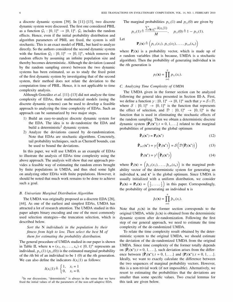
a discrete dynamic system [39]. In [11]–[13], two discretedynamic system were discussed. The first one considered PBILas a function G1 : [0, 1]n → [0, 1]n. G1 includes the randomeffects. Hence, even if the initial probability distribution andalgorithm parameters of PBIL are fixed, the system is stillstochastic. This is an exact model of PBIL, but hard to analyzedirectly. So the authors considered the second dynamic systemwith the function G2 : [0, 1]n → [0, 1]n, which removes therandom effects by assuming an infinite population size andthereby becomes deterministic. Although the deviation (causedby the random sampling errors) between the two dynamicsystems has been estimated, so as to study the fixed pointof the first dynamic system by investigating that of the secondsystem, their method does not relate the deviation to thecomputation time of PBIL. Hence, it is not applicable to timecomplexity analysis.
Although Gonzalez et al. [11]–[13] did not analyze the timecomplexity of EDAs, their mathematical models (using thediscrete dynamic systems) can be used to develop a feasibleapproach to analyzing the time complexity of EDAs. Such anapproach can be summarized by two major steps.
1) Build an easy-to-analyze discrete dynamic system forthe EDA. The idea is to de-randomize the EDA andbuild a deterministic2 dynamic system.
2) Analyze the deviations caused by de-randomization.Note that EDAs are stochastic algorithms. Concretely,tail probability techniques, such as Chernoff bounds, canbe used to bound the deviations.
In this paper, we will use UMDA as an example of EDAsto illustrate the analysis of EDAs time complexity using theabove approach. The analysis will show that our approach pro-vides a feasible way of estimating the random errors broughtby finite populations in UMDA, and thus shed some lighton analyzing other EDAs with finite populations. However, itshould be noted that much work remains to be done to achievesuch a goal.
B. Univariate Marginal Distribution Algorithm
The UMDA was originally proposed as a discrete EDA [28],[44]. As one of the earliest and simplest EDAs, UMDA hasattracted a lot of research attention. The UMDA studied in thispaper adopts binary encoding and one of the most commonlyused selection strategies—the truncation selection, which isdescribed below.
Sort the N individuals in the population by theirfitness from high to low. Then select the best M ofthem for estimating the probability distribution.
The general procedure of UMDA studied in our paper is shownin Table II, where x = (x1, x2, . . ., xn) ∈ {0, 1}n represents anindividual, pt,i(1) (pt,i(0)) is the estimated marginal probabilityof the ith bit of an individual to be 1 (0) at the tth generation.We can also define the indicators δ(xi|1) as follows:
δ(xi|1)�{
1, xi = 10, xi = 0.
2In our discussions, “deterministic” is always in the sense that we havefixed the initial values of all the parameters of the non-self-adaptive EDA.
The marginal probabilities pt,i(1) and pt,i(0) are given by
pt,i(1)�∑
x∈ξ(s)t
δ(xi|1)
M, pt,i(0)� 1− pt,i(1).
LetPt(x)�
(pt,1(x1), pt,2(x2), . . . , pt,n(xn)
)where Pt(x) is a probability vector, which is made up ofn random variables (that is because, UMDA is a stochasticalgorithm). Then the probability of generating individual x inthe tth generation is
pt(x) =n∏
i=1
pt,i(xi).
C. Analyzing Time Complexity of UMDA
The UMDA given in the former section can be analyzedfollowing the general idea presented in Section III-A. First,we define a function γ : [0, 1]n→ [0, 1]n such that γ = S ◦D,where S : [0, 1]n → [0, 1]n is the function that representsthe effect of selection, and D : [0, 1]n → [0, 1]n is thefunction that is used in eliminating the stochastic effects ofthe random sampling. Then we obtain a deterministic discretedynamic system {Pt(x∗); t = 0, 1, . . .} related to the marginalprobabilities of generating the global optimum
P0(x∗) = P0(x∗) (12)
Pt+1(x∗) = γ(
Pt(x∗))
= S(D(Pt(x∗)
))(13)
Pt(x∗) = γt(
P0(x∗))
(14)
where Pt(x) =(pt,1(x1), . . . , pt,n(xn)
)is the marginal prob-
ability vector of the deterministic system for generating anindividual x, and x∗ is the global optimum. Since UMDA isusually initialized with a uniform distribution, we considerP0(x) = P0(x) =
(12 , . . . , 1
2
)in this paper. Correspondingly,
the probability of generating an individual x is
pt(x) =n∏
i=1
pt,i(xi).
Note that pt(x) in the former section corresponds to theoriginal UMDA, while pt(x) is obtained from the deterministicdynamic system after de-randomization. Following the firststep of our general approach, we need to estimate the timecomplexity of the de-randomized UMDA.
To relate the time complexity result obtained by the deter-ministic system to the original UMDA, we should estimatethe deviation of the de-randomized UMDA from the originalUMDA. Since time complexity of the former totally dependson {Pt(x∗); t = 0, 1, . . .}, such deviation arises from the differ-ence between {Pt(x∗); t = 0, 1, . . .} and {Pt(x∗); t = 0, 1, . . .}.Ideally, we want to exactly calculate the difference betweenthe two sequences of marginal probability vectors. However,this is a non-trivial work (if not impossible). Alternatively, weresort to estimating the probabilities that the deviations aresmaller than some specific values. Two crucial lemmas forthis task are given below.
Authorized licensed use limited to: Ke Tang. Downloaded on February 13,2010 at 20:36:32 EST from IEEE Xplore. Restrictions apply.

CHEN et al.: ANALYSIS OF COMPUTATIONAL TIME OF SIMPLE ESTIMATION OF DISTRIBUTION ALGORITHMS 7
TABLE II
Univariate Marginal Distribution Algorithm (UMDA) With Truncation Selection
p0,i(xi)← Initial values (∀i = 1, . . . , n)ξ1 ← N individuals are sampled according to the distribution
p0(x) =∏n
i=1 p0,i(xi)t← 1;Repeat
ξ(s)t ← The best M individuals are selected from the N individuals in ξt (N > M)
pt,i(1)←∑
x∈ξ(s)t
δ(xi|1)
M, pt,i(0)← 1− pt,i(1) (∀i = 1, . . . , n)
ξt+1 ← N individuals are sampled according to the distributionpt(x) =
∏n
i=1 pt,i(xi)t← t + 1;
Until the Stopping Criterion is Met
Lemma 3 ([26]): Chernoff Bounds. Let X1, X2, . . . , Xk ∈{0, 1} be k independent random variables (take the value ofeither 0 or 1) with a same distribution
∀i �= j : P(Xi = 1) = P(Xj = 1)
where i, j ∈ {1, . . . , k}. Let X be the sum of those randomvariables, i.e., X =
∑ki=1 Xi, then we have:
1) ∀0 < δ < 1
P
(X < (1− δ)E[X]
)< e−E[X]δ2/2;
2) ∀δ ≤ 2e− 1
P
(X > (1 + δ)E[X]
)< e−E[X]δ2/4.
Lemma 4 ([21], [38]): Consider sampling without replace-ment from a finite population (X1, . . . , XN ) ∈ {0, 1}N . Let(Y1, . . . , YM) ∈ {0, 1}M be a sample of size M get randomlywithout replacement from the whole population, Y (M) andX(N) be the sums of the random variables in the sampleand population, respectively, i.e., Y (M) =
∑Mi=1 Yi and X(N) =∑N
i=1 Xi, then we have
P
(Y (M) − MX(N)
N≥ Mδ
)≤ e− 2Mδ2
1−(M−1)/N
< e−2Mδ2
P
(∣∣∣Y (M) − MX(N)
N
∣∣∣ > Mδ
)≤ 2e
− 2Mδ2
1−(M−1)/N
< 2e−2Mδ2
where δ ∈ [0, 1] is some constant.3
Another issue that will be involved in our further analysisis to estimate the probability of the following events:
∀t ∈ N0 : pt(x∗)⊕ pt(x∗) (15)
where ⊕ ∈ {≤,≥}. As we will show soon, they can be handledon the basis of estimation of the probabilities of deviations.Finally, before presenting the case studies in detail, it shouldbe noted that we always consider finite population sizesthroughout this paper. Although we will sometimes utilize astatement like “when the problem size becomes sufficientlylarge,” that does not mean that we assume infinite population
3The first inequality can be found in Corollary 1.1 in [38], or a similar formcan be found in [21], and the second inequality is in (3.3) in [38].
sizes, it is merely used to obtain the asymptotic order of afunction of the problem size n. The main difference is thatthe infinite population assumption implies infinite populationsizes for all problem sizes (so that the random sampling errorsare removed), while in our case the population size will beinfinite only if the problem size has become infinite.
IV. Worst Case Analysis of UMDA on the
LeadingOnes Problem
The first maximization problem we investigate is called theLeadingOnes problem, formally defined as follows:
LeadingOnes(x)�n∑
i=1
i∏j=1
xj, xj ∈ {0, 1}. (16)
The global optimum of LeadingOnes is x∗ = (1, . . . , 1).The fitness of an individual is determined by the number ofthe leading 1-bits in the individual, and it is not influencedby any bits right to the leftmost 0-bit of the individual. Thevalue of the bits right to the leftmost 0-bit will not influencethe output of fitness-based selection operators in EAs. Due tothis characteristic, a population will begin to converge to 1 ata bit if the bits left to it have almost converged to 1’s, andthus a sequential convergence phenomenon, namely Dominoconvergence [3], [36], [41], will happen.
In the literature of EDAs, the LeadingOnes problem hasbeen investigated empirically [10], but no rigorous theoreticalresult exists. This section will provide the first theoreticalresult that put a sound foundation to the time complexityanalysis of the UMDA on this problem.
First, we introduce the following concept.Definition 1 (b-Promising Individual): In the population
that contains N individuals, the b-promising individuals arethose individuals with fitness no smaller than a threshold b.
Since the UMDA adopts the truncation selection, we havethe following lemma.
Lemma 5: For the UMDA with truncation selection, thepoportion of the b-promising individuals after selection at thetth generation satisfies
Q(s)t,b =
{Qt,bN
M, Qt,b ≤ M
N
1, Qt,b > MN
(17)
Authorized licensed use limited to: Ke Tang. Downloaded on February 13,2010 at 20:36:32 EST from IEEE Xplore. Restrictions apply.

8 IEEE TRANSACTIONS ON EVOLUTIONARY COMPUTATION, VOL. 14, NO. 1, FEBRUARY 2010
where Qt,b ≤ 1 is the proportion of the b-promising individ-uals before the truncation selection.
Define the i-convergence time Ti to be the number ofgenerations for a discrete EDA to converge to the globallyoptimal value on the ith bit of the solution. It is definedformally as
Ti � min{t; pt,i(x∗i ) = 1}.
Let T0 = 0.Moreover, in the following parts of the paper, we use
the notation “ω” to demonstrate the relationship betweenthe asymptotic orders of two functions [5], [24]. Given twopositive functions of the problem size n, say f = f (n) andg = g(n), f = ω(g) holds if and only if limn→∞ g(n)/f (n) = 0.Now we reach the following theorem.
Theorem 2: Given the population sizes N = ω(n2+α log n),M = ω(n2+α log n) (where α can be any positive constant) andM = βN (β ∈ (0, 1) is some constant), for the UMDA withtruncation selection on the LeadingOnes problem, initializedwith a uniform distribution, at least with the probability of(
1− n−ω(n2+α)δ2)τ(
1− n−(
1−( 1n
)1+ α2
)2ω(1))2(n−1)τ
its FHT satisfies
τ < τ =n(
ln eMN− ln(1− δ)
)ln(1− δ) + ln
(NM
) + 2n
where δ ∈ (max{0, 1 − 2MN}, 1 − M
N) is a positive constant,
and τ represents an upper bound4 of the random variable τ.In other words, the LeadingOnes problem is EDA-easy forthe UMDA.
Proof: The basic idea of the proof is based on theapproach outlined in the former section. We first de-randomizethe UMDA. Since the LeadingOnes problem is associatedwith the domino convergence property, we can further dividethe optimization process into n stages. The ith stage startswhen all bits at the left side of the ith bit have converged to 1’s,and ends when the ith bit has converged. Suppose generationt + 1 belongs to the ith stage, then the marginal probabilitiesat the generation are
Pt+1(x∗) = γi(Pt(x∗)) =(pt,1(x∗1), . . . , pt,i−1(x∗i−1),
[Gpt,i(x∗i )], Rpt,i+1(x∗i+1), . . . , Rpt,n(x∗n)
)where x∗ = (x∗1, . . . , x
∗n) = (1, . . . , 1) is the global optimum of
the LeadingOnes problem, G = (1 − δ) NM
(δ ∈ (max{0, 1 −2MN}, 1 − M
N) is a constant), and R = (1 − η)(1 − η′) (η < 1
and η′ < 1 are positive functions of the problem size n). Weconsider three different cases in the above equation.
1) j ∈ {1, . . . , i − 1}. In the deterministic system above,the marginal probabilities pt,j(x∗j ) have converged to 1,thus at the next generation they will not change.
2) j = i. In the deterministic system above, the marginalprobability pt,i(x∗i ) is converging, and we use the factorG = (1 − δ) N
Mto demonstrate the impact of selection
4Given the values of the population sizes and the constant δ, the value of τ
is then determined by the problem size n. Thus, τ is not a random variable.
pressure on this converging marginal probability,5 whereNM
represents the influence of the selection operator (seeLemma 5).
3) j ∈ {i + 1, . . . , n}. The jth bits of individuals are notexposed to selection pressure, and we use the factor R =(1−η)(1−η′) to demonstrate the impact of genetic drift6
on these marginal probabilities.
In Case 3, we consider the jth marginal probability p.,j(x∗j )(j ∈ {i + 1, . . . , n}) which is not affected by the selectionpressure. This is rather pessimistic, because the UMDA tendsto preserve the value of x∗j = 1 that leads to higher fitness, andthus tends to increase p.,j(x∗j ). Utilizing the idea mentionedin (15), we will study the time complexity of the UMDAby studying the above deterministic system, and estimatethe deviation between the deterministic system and the realUMDA in terms of the probability that the stochastic marginalprobabilities of the UMDA are bounded by the correspondingdeterministic marginal probabilities of the deterministic sys-tem. Before our analysis, we first provide the formal definitionof the deterministic system.
With P0(x∗) =(
12 , . . . , 1
2
), we have
Pt(x∗) = γt−Ti−1i
(PTi−1 (x∗)
)where Ti−1 < t ≤ Ti (i = 1, . . . , n). Since {γi}ni=1 de-randomizes the whole optimization process, {Ti}ni=1 in theabove equation are no longer random variables. For the sakeof clarity, we rewrite the above equation as
Pt(x∗) = γt−Ti−1i
(PTi−1
(x∗))
where Ti−1 < t ≤ Ti (i = 1, . . . , n). As we will showimmediately, Ti (1 ≤ i ≤ n) is an upper bound of the randomvariable Ti with some probability. Since Tn ≥ τ, our taskfinally becomes calculating the Tn and the probability that Tn
holds as an upper bound of Tn.Now we present the proof in detail. First, we estimate T1
and T1 for the UMDA, which is the first stage of our analysis.Consider the 1-promising individuals. Note that the first bits ofthe 1-promising individuals are 1’s. The sampling procedureof the UMDA can be considered as a large number of eventsresulting in either 0 or 1. Hence, when pt−1,1(1) ≤ M
N(1−δ) , forthe sampling procedure of the UMDA, by noting Lemma 5,we can apply Chernoff bounds to obtain the following:
P
(Mpt,1(1) ≥ (1− δ)pt−1,1(1)N | pt−1,1(1) ≤ M
N(1− δ)
)
> 1− e−pt−1,1(1)N
2 δ2
where N = ω(n2 log n), thus the probability above is super-polynomially close to 1, i.e., an overwhelming probability. An
5The notation “[ ]” can be interpreted as follows: given a > 1, [a] = 1;given a ∈ (0, 1), [a] = a. For the sake of brevity, we will omit this notation butimplicitly restrict the value of a probability not to exceed 1 in the followingparts of the paper.
6When there is no selection pressure, the proportion of alleles in apopulation with finite genes will fluctuate due to the errors brought by randomsampling. For more details, one can refer to [6], [41].
Authorized licensed use limited to: Ke Tang. Downloaded on February 13,2010 at 20:36:32 EST from IEEE Xplore. Restrictions apply.

CHEN et al.: ANALYSIS OF COMPUTATIONAL TIME OF SIMPLE ESTIMATION OF DISTRIBUTION ALGORITHMS 9
TABLE III
Calculation of Probability That pt,1(1) Is Lower Bounded by pt,1(1)
P
(pt,1(1) ≥ pt,1(1) | p0,1(1) = p0,1(1)
)=
∑∀t′<t:at′ ∈
{0, 1
M, 2M
,···,1}P(
pt,1(1) ≥ Gtp0,1(1), pt−1,1(1) = at−1, · · · , p1,1(1) = a1 | p0,1(1) = p0,1(1))
> P
(pt,1(1) ≥ Gpt−1,1(1), · · · , p1,1(1) ≥ Gp0,1(1) | p0,1(1) = p0,1(1)
)= P(
pt−1,1(1) ≥ Gpt−2,1(1), · · · , p1,1(1) ≥ Gp0,1(1) | p0,1(1) = p0,1(1))
P
(pt,1(1) ≥ Gpt−1,1(1) | pt−1,1(1) ≥ Gpt−2,1(1), · · · , p1,1(1) ≥ Gp0,1(1), p0,1(1) = p0,1(1)
)= P(
p1,1(1) ≥ Gp0,1(1) | p0,1(1) = p0,1(1))
t∏k=2
P
(pk,1(1) ≥ Gpk−1,1(1) | pk−1,1(1) ≥ Gpk−2,1(1), · · · , p1,1(1) ≥ Gp0,1(1), p0,1(1) = p0,1(1)
)
= P(
p1,1(1) ≥ Gp0,1(1) | p0,1(1) = p0,1(1))
t∏k=2
P
(pk,1(1) ≥ Gpk−1,1(1) | pk−1,1(1) ≥ pk−1,1(1) = Gk−1p0,1(1)
)
>
t∏k=1
(1− e−pk−1,1(1)Nδ2/2
)=
t∏k=1
(1− e−Gk−1p0,1(1)Nδ2/2
)>
(1− e−p0,1(1)Nδ2/2
)t
TABLE IV
Calculation of Probability That T1 Is Upper Bounded by T1
P
(T1 ≤ T1 | p0,1(1) = p0,1(1)
)(18)
> P
(pT1−1,1(1) ≥ M
N(1− δ)| p0,1(1) = p0,1(1)
)(1− e−
p0,1(1)N2 δ2
)(19)
> P
(pT1−1,1(1) ≥ pT1−1,1(1) = GT1−1p0,1(1) >
M
N(1− δ)| p0,1(1) = p0,1(1)
)(1− e−
p0,1(1)N2 δ2
)> P
(pT1−1,1(1) ≥ pT1−1,1(1) | p0,1(1) = p0,1(1), pT1−1,1(1) >
M
N(1− δ)
)·P(
pT1−1,1(1) >M
N(1− δ)| p0,1(1) = p0,1(1)
)(1− e−
p0,1(1)N2 δ2
)
TABLE V
Bounding N(s)t,j (x∗j ) From Below With an Overwhelming Probability
P
(N
(s)t,j (x∗j ) > (1− η′)
(1− η)pt−1,j(x∗j )N
NM | Nt,j(x∗j ) ≥
(1−(
1
n
)1+ α2)
pt−1,j(x∗j )N, pt−1,j(xj)
)
= P
((1− η)pt−1,j(x∗j )N
NM −N
(s)t,j (x∗j ) < η′
(1− η)pt−1,j(x∗j )N
NM | Nt,j(x∗j ) ≥
(1−(
1
n
)1+ α2)
pt−1,j(x∗j )N, pt−1,j(x∗j )
)> 1− 2e
−2(1−η)2p2t−1,j
(x∗j
)η′2M
Authorized licensed use limited to: Ke Tang. Downloaded on February 13,2010 at 20:36:32 EST from IEEE Xplore. Restrictions apply.

10 IEEE TRANSACTIONS ON EVOLUTIONARY COMPUTATION, VOL. 14, NO. 1, FEBRUARY 2010
TABLE VI
Calculation of the Joint Probability That T1 Is Bounded Above by T2
P
(T2 ≤ T2, T1 ≤ T1, pT1,2(1) ≥ pT1,2(1) >
1
e| p0,1(1) = p0,1(1), p0,2(1) = p0,2(1)
)(20)
> P
(pT2−1,2(1) ≥ M
N(1− δ)| p0,1(1) = p0,1(1), p0,2(1) = p0,2(1), T1 ≤ T1, pT1,2(1) ≥ pT1,2(1) >
1
e
)
·(
1− e−ω(n2+α log n)
2eδ2)T1(
1− n−(
1−( 1n )
1+ α2)2
ω(1)
)2T1(1− e−
pT1 ,2(1)N
2 δ2)
(21)
> P
(pT2−1,2(1) ≥ pT2−1,2(1) = GT2−T1−1pT1,2(1) >
M
N(1− δ)| pT1,1(1) = 1, pT1,2(1) ≥ pT1,2(1) >
1
e
)
·(
1− e−ω(n2+α log n)
2eδ2)T1(
1− n−(
1−( 1n )
1+ α2)2
ω(1)
)2T1(1− e−
pT1 ,2(1))N
2 δ2)
> P
(pT2−1,2(1) ≥ pT2−1,2(1) | pT1,1(1) = 1, pT1,2(1) ≥ pT1,2(1) >
1
e, pT2−1,2(1) >
M
N(1− δ)
)(22)
P
(pT2−1,2(1) >
M
N(1− δ)| pT1,1(1) = 1, pT1,2(1) ≥ pT1,2(1) >
1
e
)
·(
1− e−ω(n2+α log n)
2eδ2)T1(
1− n−(
1−( 1n )
1+ α2)2
ω(1)
)2T1(1− e−
ω(n2+α log n)2e
δ2)
TABLE VII
Bounding N(s)t,q (x∗q) From Above With an Overwhelming Probability
P
(N
(s)t,q (x∗q) < (1 + η′)
(1 + η)pt−1,q(x∗q)N
NM | Nt,q(x∗q) ≤
(1 +(
1
n
)1+ α2)
pt−1,q(x∗q)N, pt−1,q(x∗q)
)
= P
(N
(s)t,q (x∗q)− (1 + η)pt−1,q(x∗q)N
NM < η′
(1 + η)pt−1,q(x∗q)N
NM | Nt,q(x∗q) ≤
(1 +(
1
n
)1+ α2)
pt−1,q(x∗q)N, pt−1,q(x∗q)
)> 1− e
−2(1+η)2p2t−1,q
(x∗q )η′2M(23)
equivalent form of the equation above is
P
(pt,1(1) ≥ (1− δ)pt−1,1(1)N
M| pt−1,1(1) ≤ M
N(1−δ)
)> 1− e−
pt−1,1(1)N
2 δ2
which demonstrates with an overwhelming probability themarginal probability pt,1(1) is lower bounded by Gpt−1,1(1) =(1 − δ)pt−1,1(1)N
M. Furthermore, given pt,1(1) = Gtp0,1(1) and
G > 1, we can obtain the inequality in Table III.We now study the distribution of T1. Considering the
probability that T1 is bounded by a value, say T1: givenT1 < T1, then according to Lemma 5, at the (T1 − 1)thgeneration, the marginal probability pT1−1,1(1) should be atleast M
N(1−δ) . The above proposition is presented in Table IV,
where in (19) the factor (1 − e−p0,1(1)N
2 δ2) is added since we
apply Chernoff bounds once at the end of the (T1 − 1)thgeneration and obtain the probability that pT1,1(1) = 1, underthe condition pT1−1,1(1) ≥ M
N(1−δ) . Now let us consider thefollowing item. Noting that pT1−1,1(1) is deterministic, we
know
P
(pT1−1,1(1) >
M
N(1− δ)| p0,1(1) = p0,1(1)
)(24)
must be either 0 or 1, and we need to find the value of T1 thatmakes the probability above 1. Given that p0,1(1) = 1
2 , thecondition that ∀t < T1− 1 : M
N(1−δ) > pt,1(1) > (1− δ) pt−1,1(1)NM
and Lemma 5 together imply the following inequalities.
GT1−2p0,1(1) = (1− δ)T1−2
(N
M
)T1−2
p0,1(1)
<M
N(1− δ)
GT1−1p0,1(1) = (1− δ)T1−1
(N
M
)T1−1
p0,1(1)
≥ M
N(1− δ).
Solving the inequalities above, we get
T1 ≤ln 2M
N− ln(1− δ)
ln(1− δ) + ln(
NM
) + 2
Authorized licensed use limited to: Ke Tang. Downloaded on February 13,2010 at 20:36:32 EST from IEEE Xplore. Restrictions apply.

CHEN et al.: ANALYSIS OF COMPUTATIONAL TIME OF SIMPLE ESTIMATION OF DISTRIBUTION ALGORITHMS 11
where δ ∈ (max{0, 1 − 2MN}, 1 − M
N) is a constant, and it
is easy to show that T1 = (1). On the other hand, recallthe inequalities in Table III, we can continue to estimate thecorresponding probability mentioned in (18)
P
(T1 ≤ T1 | p0,1(1) = p0,1(1)
)> P
(pT1−1,1(1) ≥ pT1−1,1(1) | p0,1(1) = p0,1(1)
)·(
1− e−p0,1(1)N
2 δ2)
>(
1− e−p0,1(1)N
2 δ2)T1
. (25)
The analysis above tells us, the probability to which themarginal probability converges before the T1th generation
(T1 < T1) is at least(
1− e−N4 δ2)T1
. Since N = ω(n2+α log n),
M = βN (β ∈ (0, 1) is a constant) and T1 is polynomial in theproblem size n, we know that the probability is overwhelming.
At every stage, the bits on the right-hand side of thecurrently converging bit are not exposed to selection pressure.However, we should still consider the errors brought by therepeated sampling procedures in UMDA, which is related tothe genetic drift [6], [41].
Take the first stage as an example. The jth bit (j = 2, . . . , n)is affected by genetic drift. First, we utilize Chernoff boundsto study the deviations brought by the random samplingprocedures of the UMDA
P
(Nt,j(x∗j ) ≥ (1− η)pt−1,j(x∗j )N | pt−1,j(x∗j )
)
> 1− e−pt−1,j (1)N
2 η2
where η is a parameter that controls the size of deviation, andNt,j(xj) is the number of individuals that takes the value xj
in their jth bit in the population before selection, ξt . Here we
set η =(
1n
)1+ α2, and obtain
P
(Nt,j(x∗j ) ≥
(1−
(1
n
)1+ α2)pt−1,j(x∗j )N | pt−1,j(x∗j )
)
> 1− e−pt−1,j (x∗
j)ω(log n)
2 = 1− n−pt−1,j (x∗
j)ω(1)
2 .
Second, we further consider the selection procedure, sinceit may also bring some deviations. In our worst case analysis,the jth bits of individuals are considered to not be exposedto the selection pressure, then for these bits the selectionprocedure can be regarded as get a simple random sampleof M individuals from a finite population with N individuals[34]. More precisely, since one individual cannot be selectedmore than once by the truncation selection, this procedure isknown as random sampling without replacement from a finitepopulation [34] in the field of statistics. From Lemma 4, wecan bound from below the probability such that the number ofindividuals taking the value x∗j on their jth bits after selection[denoted by N
(s)t,j (x∗j )] is lower bounded, which is shown by the
inequalities presented in Table V, where η′ is a parameter thatcontrols the size of deviation, and N
(s)t,j (x∗j ) = pt,j(x∗j )M. By
setting η′ = η =(
1n
)1+ α2, since M = ω(n2+α log n) we obtain
P
(pt,j(x∗j ) ≥
(1−
(1
n
)1+ α2)2
pt−1,j(x∗j ) | pt−1,j(x∗j )
)
>(
1− n−pt−1,j(x∗
j)ω(1))
·(
1− n−(
1−( 1n
)1+ α2
)2p2
t−1,j(x∗
j)ω(1))
>(
1− n−(
1−( 1n
)1+ α2
)2p2
t−1,j(x∗
j)ω(1))2
.
Since the factor R =(
1−(
1n
)1+ α2)2
< 1, for ∀j = 2 . . . , n
and t = 1, . . . , T1, similar to the analysis shown in Table III,we further obtain
P
(pt,j(x∗j ) ≥
(1−
(1n
)1+ α2)2t
p0,j(x∗j )
| p0,j(x∗j ) = p0,j(x∗j )
)
>
(1− n
−(
1−( 1n
)1+ α2
)2p2
t−1,j(x∗
j)ω(1))2t
. (26)
Given any t = O(n), according to the definition of thedeterministic system, we know
pt,j(x∗j ) ≥(
1−(1
n
)1+ α2)O(n)
p0,j(x∗j ) >1
e
holds. The above inequality implies that within the numberof generations t = O(n), the probability in (26) is an over-whelming one.
To generalize the above analysis to other stages, let usconsider the ith (i ∈ {2, . . . , n}) stage is about to start.Due to the genetic drift, the marginal probability pt,j(x∗j )(j ∈ {i, . . . , n}) has dropped to a lower level than the initialvalue 1
2 by multiplying the factor Rt . We concern the value ofpt,i(x∗i ). For any t = O(n), similar to (26), the probability thatpt,i(x∗i ) maintains a level of
pt,i(x∗i ) ≥
(1−
(1
n
)1+ α2)O(n)
p0,i(x∗i ) >
1
e(27)
is super-polynomially close to 1 (an overwhelming pro-bability).
According to (27), we know that pt,i(x∗i ) is above 1e
with anoverwhelming probability. Consequently, the joint probabilitythat the first bit has converged to 1 and the genetic drift cannotreduce pT1,2(1) to be smaller than 1
eby the end of the first
stage is(1− e−
ω(n2+α log n)2e
δ2)T1(
1− n−(
1−( 1n
)1+ α2
)2ω(1))2T1
(28)
which is again an overwhelming probability. Now we havefinished the analysis of the first stage.
As the dynamic system we described at the beginning ofthe proof, in the second stage, for T1 < t ≤ T2, we have
pt,2(1) = Gpt−1,2(1).
Given T1 and the corresponding marginal probabilities, weconsider the joint probability that T2 is bounded above byT2 by inequalities presented in Table VI.
Authorized licensed use limited to: Ke Tang. Downloaded on February 13,2010 at 20:36:32 EST from IEEE Xplore. Restrictions apply.
12 IEEE TRANSACTIONS ON EVOLUTIONARY COMPUTATION, VOL. 14, NO. 1, FEBRUARY 2010
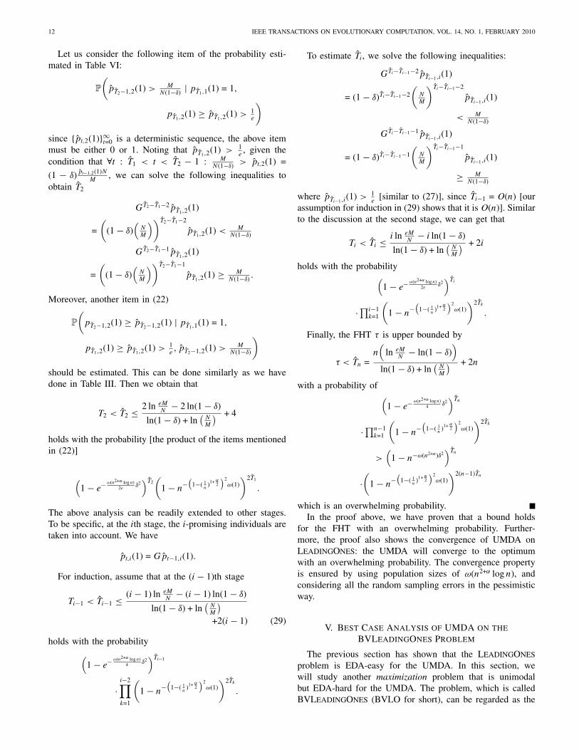
Let us consider the following item of the probability esti-mated in Table VI:
P
(pT2−1,2(1) > M
N(1−δ) | pT1,1(1) = 1,
pT1,2(1) ≥ pT1,2(1) > 1e
)
since {pt,2(1)}∞t=0 is a deterministic sequence, the above itemmust be either 0 or 1. Noting that pT1,2(1) > 1
e, given the
condition that ∀t : T1 < t < T2 − 1 : MN(1−δ) > pt,2(1) =
(1 − δ) pt−1,2(1)NM
, we can solve the following inequalities toobtain T2
GT2−T1−2pT1,2(1)
=
((1− δ)
(NM
))T2−T1−2
pT1,2(1) < MN(1−δ)
GT2−T1−1pT1,2(1)
=
((1− δ)
(NM
))T2−T1−1
pT1,2(1) ≥ MN(1−δ) .
Moreover, another item in (22)
P
(pT2−1,2(1) ≥ pT2−1,2(1) | pT1,1(1) = 1,
pT1,2(1) ≥ pT1,2(1) > 1e, pT2−1,2(1) > M
N(1−δ)
)
should be estimated. This can be done similarly as we havedone in Table III. Then we obtain that
T2 < T2 ≤2 ln eM
N− 2 ln(1− δ)
ln(1− δ) + ln(
NM
) + 4
holds with the probability [the product of the items mentionedin (22)]
(1− e−
ω(n2+α log n)2e
δ2)T2(
1− n−(
1−( 1n
)1+ α2
)2ω(1))2T1
.
The above analysis can be readily extended to other stages.To be specific, at the ith stage, the i-promising individuals aretaken into account. We have
pt,i(1) = Gpt−1,i(1).
For induction, assume that at the (i− 1)th stage
Ti−1 < Ti−1 ≤(i− 1) ln eM
N− (i− 1) ln(1− δ)
ln(1− δ) + ln(
NM
)+2(i− 1) (29)
holds with the probability(1− e−
ω(n2+α log n)4 δ2
)Ti−1
·i−2∏k=1
(1− n
−(
1−( 1n
)1+ α2
)2ω(1))2Tk
.
To estimate Ti, we solve the following inequalities:
GTi−Ti−1−2pTi−1,i(1)
= (1− δ)Ti−Ti−1−2
(NM
)Ti−Ti−1−2
pTi−1,i(1)
< MN(1−δ)
GTi−Ti−1−1pTi−1,i(1)
= (1− δ)Ti−Ti−1−1
(NM
)Ti−Ti−1−1
pTi−1,i(1)
≥ MN(1−δ)
where pTi−1,i(1) > 1
e[similar to (27)], since Ti−1 = O(n) [our
assumption for induction in (29) shows that it is O(n)]. Similarto the discussion at the second stage, we can get that
Ti < Ti ≤i ln eM
N− i ln(1− δ)
ln(1− δ) + ln(
NM
) + 2i
holds with the probability(1− e−
ω(n2+α log n)2e
δ2)Ti
·∏i−1k=1
(1− n
−(
1−( 1n
)1+ α2
)2ω(1))2Tk
.
Finally, the FHT τ is upper bounded by
τ < Tn =n(
ln eMN− ln(1− δ)
)ln(1− δ) + ln
(NM
) + 2n
with a probability of (1− e−
ω(n2+α log n)4 δ2
)Tn
·∏n−1k=1
(1− n
−(
1−( 1n
)1+ α2
)2ω(1))2Tk
>(
1− n−ω(n2+α)δ2)Tn
·(
1− n−(
1−( 1n
)1+ α2
)2ω(1))2(n−1)Tn
which is an overwhelming probability.In the proof above, we have proven that a bound holds
for the FHT with an overwhelming probability. Further-more, the proof also shows the convergence of UMDA onLeadingOnes: the UMDA will converge to the optimumwith an overwhelming probability. The convergence propertyis ensured by using population sizes of ω(n2+α log n), andconsidering all the random sampling errors in the pessimisticway.
V. Best Case Analysis of UMDA on the
BVLeadingOnes Problem
The previous section has shown that the LeadingOnes
problem is EDA-easy for the UMDA. In this section, wewill study another maximization problem that is unimodalbut EDA-hard for the UMDA. The problem, which is calledBVLeadingOnes (BVLO for short), can be regarded as the
Authorized licensed use limited to: Ke Tang. Downloaded on February 13,2010 at 20:36:32 EST from IEEE Xplore. Restrictions apply.
CHEN et al.: ANALYSIS OF COMPUTATIONAL TIME OF SIMPLE ESTIMATION OF DISTRIBUTION ALGORITHMS 13
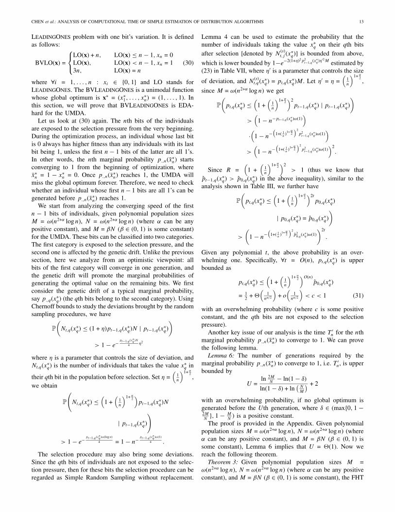
LeadingOnes problem with one bit’s variation. It is definedas follows:
BVLO(x) =
⎧⎨⎩
LO(x) + n, LO(x) ≤ n− 1, xn = 0LO(x), LO(x) < n− 1, xn = 13n, LO(x) = n
(30)
where ∀i = 1, . . . , n : xi ∈ {0, 1} and LO stands forLeadingOnes. The BVLeadingOnes is a unimodal functionwhose global optimum is x∗ = (x∗1, . . . , x
∗n) = (1, . . . , 1). In
this section, we will prove that BVLeadingOnes is EDA-hard for the UMDA.
Let us look at (30) again. The nth bits of the individualsare exposed to the selection pressure from the very beginning.During the optimization process, an individual whose last bitis 0 always has higher fitness than any individuals with its lastbit being 1, unless the first n− 1 bits of the latter are all 1’s.In other words, the nth marginal probability p.,n(x∗n) startsconverging to 1 from the beginning of optimization, wherex∗n = 1 − x∗n = 0. Once p.,n(x∗n) reaches 1, the UMDA willmiss the global optimum forever. Therefore, we need to checkwhether an individual whose first n− 1 bits are all 1’s can begenerated before p.,n(x∗n) reaches 1.
We start from analyzing the converging speed of the firstn − 1 bits of individuals, given polynomial population sizesM = ω(n2+α log n), N = ω(n2+α log n) (where α can be anypositive constant), and M = βN (β ∈ (0, 1) is some constant)for the UMDA. These bits can be classified into two categories.The first category is exposed to the selection pressure, and thesecond one is affected by the genetic drift. Unlike the previoussection, here we analyze from an optimistic viewpoint: allbits of the first category will converge in one generation, andthe genetic drift will promote the marginal probabilities ofgenerating the optimal value on the remaining bits. We firstconsider the genetic drift of a typical marginal probability,say p.,q(x∗q) (the qth bits belong to the second category). UsingChernoff bounds to study the deviations brought by the randomsampling procedures, we have
P
(Nt,q(x∗q) ≤ (1 + η)pt−1,q(x∗q)N | pt−1,q(x∗q)
)
> 1− e−pt−1,q (x∗q )N
4 η2
where η is a parameter that controls the size of deviation, andNt,q(x∗q) is the number of individuals that takes the value x∗q in
their qth bit in the population before selection. Set η =(
1n
)1+ α2,
we obtain
P
(Nt,q(x∗q) ≤
(1 +(
1n
)1+ α2)pt−1,q(x∗q)N
| pt−1,q(x∗q)
)
> 1− e−pt−1,q (x∗q )ω(log n)
4 = 1− n−pt−1,q (x∗q )ω(1)
4 .
The selection procedure may also bring some deviations.Since the qth bits of individuals are not exposed to the selec-tion pressure, then for these bits the selection procedure can beregarded as Simple Random Sampling without replacement.
Lemma 4 can be used to estimate the probability that thenumber of individuals taking the value x∗q on their qth bitsafter selection [denoted by N
(s)t,j (x∗q)] is bounded from above,
which is lower bounded by 1−e−2(1+η)2p2
t−1,q(x∗q)η′2M estimated by
(23) in Table VII, where η′ is a parameter that controls the size
of deviation, and N(s)t,q(x∗q) = pt,q(x∗q)M. Let η′ = η =
(1n
)1+ α2,
since M = ω(n2+α log n) we get
P
(pt,q(x∗q) ≤
(1 +(
1n
)1+ α2)2
pt−1,q(x∗q) | pt−1,q(x∗q)
)
>(
1− n−pt−1,q(x∗q)ω(1))
·(
1− n−(
1+( 1n
)1+ α2
)2p2
t−1,q(x∗q)ω(1)
)>(
1− n−(
1+( 1n
)1+ α2
)2p2
t−1,q(x∗q)ω(1)
)2.
Since R =(
1 +(
1n
)1+ α2)2
> 1 (thus we know thatpt−1,q(x∗q) > p0,q(x∗q) in the above inequality), similar to theanalysis shown in Table III, we further have
P
(pt,q(x∗q) ≤
(1 +(
1n
)1+ α2)2t
p0,q(x∗q)
| p0,q(x∗q) = p0,q(x∗q)
)
>
(1− n
−(
1+( 1n
)1+ α2
)2p2
0,q(x∗q)ω(1)
)2t
.
Given any polynomial t, the above probability is an over-whelming one. Specifically, ∀t = O(n), pt,q(x∗q) is upperbounded as
pt,q(x∗q) ≤(
1 +(
1n
)1+ α2)O(n)
p0,q(x∗q)
= 12 +
(1
nα/2
)+ o(
1nα/2
)< c < 1 (31)
with an overwhelming probability (where c is some positiveconstant, and the qth bits are not exposed to the selectionpressure).
Another key issue of our analysis is the time T ′n for the nthmarginal probability p.,n(x∗n) to converge to 1. We can provethe following lemma.
Lemma 6: The number of generations required by themarginal probability p.,n(x∗n) to converge to 1, i.e. T ′n, is upperbounded by
U =ln 2M
N− ln(1− δ)
ln(1− δ) + ln(
NM
) + 2
with an overwhelming probability, if no global optimum isgenerated before the Uth generation, where δ ∈ (max{0, 1 −2MN}, 1− M
N) is a positive constant.
The proof is provided in the Appendix. Given polynomialpopulation sizes M = ω(n2+α log n), N = ω(n2+α log n) (whereα can be any positive constant), and M = βN (β ∈ (0, 1) issome constant), Lemma 6 implies that U = (1). Now wereach the following theorem.
Theorem 3: Given polynomial population sizes M =ω(n2+α log n), N = ω(n2+α log n) (where α can be any positiveconstant), and M = βN (β ∈ (0, 1) is some constant), the FHT
Authorized licensed use limited to: Ke Tang. Downloaded on February 13,2010 at 20:36:32 EST from IEEE Xplore. Restrictions apply.

14 IEEE TRANSACTIONS ON EVOLUTIONARY COMPUTATION, VOL. 14, NO. 1, FEBRUARY 2010
of the UMDA with truncation selection on the BVLeadin-
gOnes problem is infinity with an overwhelming probability.In other words, the UMDA with truncation selection cannotfind the optimum of the BVLeadingOnes problem with anoverwhelming probability.
Proof: We have proven that the number of generationsrequired for p.,n(x∗n) to reach 1 (denoted by T ′n) is upperbounded by a constant function U with an overwhelmingprobability, under the condition that no global optimum isgenerated before the Uth generation. We now further provethat the probability that no global optimum is generated beforethe Uth generation is also overwhelming.
As mentioned before, we classify the first n − 1 bits ofindividuals into two categories. The first category, which con-tains the bits being exposed to the selection, further containstwo types of bits. The first type contains the bits which havealready converged to the optimal values, and the second typecontains the bits that are exposed to the selection pressurebut have not converged to the optimal values yet. In our bestcase analysis, for the bits of the second type, we consider thatonly one generation is needed for the corresponding marginalprobabilities (to the optimal values) to converge. In otherwords, before the Uth generation, the marginal probabilities(of the first n− 1 bits of individuals) are either 1 or no morethan the constant c. Noting that U = (1), according to (31),c ∈ ( 1
2 , 1), and it demonstrates the result of genetic drift withinO(n) generations.
From an optimistic viewpoint, we further consider that inevery generation, besides the marginal probability p.,n(x∗n), atmost log2 n other marginal probabilities7 are also convergingwith an overwhelming probability. log2 n is used here becausethe joint probability of generating log2 n consecutive 1’s (so asto produce the selection pressure on the corresponding bits) bylog2 n non-converged marginal probabilities is no more thanclog2 n, which is super-polynomially small.
The above result implies that the probability of gener-ating the global optimum in one generation is also super-polynomially small. Noting that U = (1), then the probabilityof generating the optimum before the Uth generation is alsosuper-polynomially small. Combining this probability withthe conditional probability mentioned in Lemma 6, we knowthat the joint probability that no global optimum is generatedbefore the Uth generation, and p.,n(x∗n) converges to 1 no laterthan the Uth generation, is super-polynomially close to 1,i.e., an overwhelming probability. Combining with the factthat once the nth marginal probability p.,n(x∗n) has alreadyconverged to 0, the probability of finding the optimum willdrop to 0, we have proven the theorem.
According to Theorem 1, given polynomial population sizesM = ω(n2+α log n) and N = ω(n2+α log n) (M = βN, β ∈(0, 1) is a constant.), BVLeadingOnes is EDA-hard for theUMDA.
For the sake of consistence, we also provide the formaldescription of the deterministic dynamic system utilized inthis section. Considering the ith stage (i ≤ min{T ′n, n−1
log2 n})
7For the sake of brevity, we assume that log2 n is an integer and thus omitthe notation “� �.”
which starts when all the marginal probabilities p.,k(x∗k) (k ≤(i − 1) log2 n}) have just converged to 1 and ends when allthe marginal probabilities p.,j(x∗j ) (j ≤ i log2 n) have justconverged to 1, we can obtain Pt+1(x∗) by defining γi asfollows.
Pt+1(x∗) = γi(Pt(x∗)) =(pt,1(x∗1), . . . , pt,(i−1) log2 n(x∗
(i−1) log2 n), 1, . . . , 1,
Rpt,i log2 n+1(x∗i log2 n+1
), . . . , Rpt,n−1(x∗n−1),
1−G(1− pt,n(x∗n))
)
where R = (1 + η)(1 + η′) (η < 1 and η′ < 1 are positivefunctions of the problem size n), and G = (1 − δ) N
M(δ ∈
(max{0, 1− 2MN}, 1− M
N) is a constant). In the above equation,
we consider four different cases.1) j ∈ {1, . . . , (i − 1) log2 n}. In the deterministic system
above, the marginal probabilities pt,j(x∗j ) have con-verged to 1, thus at the next generation they will notchange.
2) j ∈ {(i− 1) log2 n + 1, . . . , i log2 n}. In the deterministicsystem above, the marginal probabilities pt,j(x∗j ) areconverging to the optimum, and they will converge inone generation in the best case analysis.
3) j ∈ {i log2 n + 1, . . . , n− 1}. The jth bits of individualsare not exposed to selection pressure, and we use thefactor R = (1 + η)(1 + η′) to demonstrate the impact ofgenetic drift in the deterministic system above.
4) j = n. The marginal probability pt,n(x∗n) = 1 − pt,n(x∗n)is converging, and we use the factor G = (1 − δ) N
M
to demonstrate the impact of selection pressure onthis converging marginal probability in the determin-istic system above, which is a best case style forpt,n(x∗n).
With P0(x∗) =(
12 , . . . , 1
2
), noting that one stage actually
refers to one generation (thus i = t), we have
Pt(x∗) = γt ◦ γt−1 . . . ◦ γ1
(P0(x∗)
)where t ≤ min
{T ′n,
n−1log2 n
}. Since {γi}ti=1 de-randomizes the
whole optimization process, T ′n in the above equation is nolonger random variable. For the sake of clarity, we rewrite theabove equation as
Pt(x∗) = γt ◦ γt−1 . . . ◦ γ1
(P0(x∗)
)where t ≤ min
{T ′n,
n−1log2 n
}≤ min
{U, n−1
log2 n
}.
VI. A Modified UMDA: Relaxation by Margins
So far we have seen both EDA-easy and EDA-hard prob-lems for the UMDA. This section will analyze more in-depththe relationship between EDA-hardness and the algorithms.The BVLeadingOnes problem, which has proven to beEDA-hard for the UMDA with finite populations, will beemployed as the target problem in this section. We will showthat a simple “relaxed” version of UMDA with truncation
Authorized licensed use limited to: Ke Tang. Downloaded on February 13,2010 at 20:36:32 EST from IEEE Xplore. Restrictions apply.
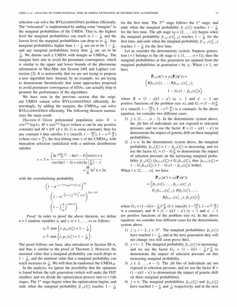
CHEN et al.: ANALYSIS OF COMPUTATIONAL TIME OF SIMPLE ESTIMATION OF DISTRIBUTION ALGORITHMS 15
selection can solve the BVLeadingOnes problem efficiently.The “relaxation” is implemented by adding some “margins” tothe marginal probabilities of the UMDA. That is, the highestlevel the marginal probabilities can reach is 1 − 1
Mand the
lowest level the marginal probabilities can drop to is 1M
. Anymarginal probabilities higher than 1− 1
Mare set to be 1− 1
M,
and any marginal probabilities lower than 1M
are set to be1M
. We denote such a UMDA with margin as UMDAM . Themargins here aim to avoid the premature convergence, whichis similar to the upper and lower bounds of the pheromoneinformation in Max-Min Ant System [40] and Laplace cor-rection [2]. It is noteworthy that we are not trying to proposea new algorithm here. Instead, by an example, we are tryingto demonstrate theoretically that some approaches proposedto avoid premature convergence of EDAs, can actually help topromote the performance of the algorithms.
We have seen in the previous section that the origi-nal UMDA cannot solve BVLeadingOnes efficiently. In-terestingly, by adding the margins, the UMDAM can solveBVLeadingOnes efficiently. The following theorem summa-rizes the main result.
Theorem 4: Given polynomial population sizes N =ω(n2+α log n), M = ω(n2+α log n) (where α can be any positiveconstant) and M = βN (β ∈ (0, 1) is some constant), then forany constant δ that satisfies δ ∈ (max{0, 1− 2M
N}, 1− e
1ε(n) M
N)
(where ε(n) = Mn
), the first hitting time τ of the UMDAM withtruncation selection (initialized with a uniform distribution)satisfies
τ < τ =
(ln e(M−1)
N− ln(1− δ)
)nε(n) + n
ε(n) ln(1− δ) + ε(n) ln(
NM
)− 1
+M
Nln2 n + 2n
with the overwhelming probability(1− n−e−1/ε(n)ω(n2+α)δ2/2e
)2τ
·(
1− n−(
1−( 1n
)1+ α2
)2ω(1))2(n−1)τ
·(
1−(1
e
)ω(ln n))
.
Proof: In order to proof the above theorem, we definen + 1 random variables t0 and ti (i = 1, . . . , n) as follows:
t0 � min{
t; pt,n(x∗n) = 1− 1M
}ti � min
{t; pt,i(x∗i ) = 1− 1
M
}.
The proof follows our basic idea introduced in Section III-A,and thus is similar to the proof of Theorem 2. However, themaximal value that a marginal probability can reach drops to1− 1
M, and the minimal value that a marginal probability can
reach increases to 1M
. We will then de-randomize the UMDAM .In the analysis, we ignore the possibility that the optimum
is found before the t0th generation (which will make the FHTsmaller), and we divide the optimization process into (n+ 1)thstages. The 1st stage begins when the optimization begins, andends when the marginal probability p.,n(x∗n) reaches 1 − 1
M
for the first time. The 2nd stage follows the 1st stage, andends when the marginal probability p.,1(x∗1) reaches 1 − 1
M
for the first time. The qth stage (q ∈ {2, . . . , n}) begins whenthe marginal probability p.,q−2(x∗q−2) reaches 1 − 1
Mfor the
first time, and ends when the marginal probability p.,q−1(x∗q−1)reaches 1− 1
Mfor the first time.
Let us consider the deterministic system. Suppose genera-tion t + 1 belongs to the ith stage (i ∈ {1, . . . , n + 1}), then themarginal probabilities at this generation are updated from themarginal probabilities at generation t by γi. When i = 1, wehave
Pt+1(x∗) = γ1(Pt(x∗)) =(Rpt,1(x∗1), . . . , Rpt,n−1(x∗n−1),
1−G1(1− pt,n(x∗n)))
where R = (1 − η)(1 − η′) (η < 1 and η′ < 1 arepositive functions of the problem size n), and G1 = (1− δ) N
M
(δ ∈ (max{0, 1− 2MN}, 1− e
1ε(n) M
N) is a constant). In the above
equation, we consider two different cases.1) j ∈ {1, . . . , n − 1}. In the deterministic system above,
the jth bits of individuals are not exposed to selectionpressure, and we use the factor R = (1 − η)(1 − η′) todemonstrate the impact of genetic drift on these marginalprobabilities.
2) j = n. In the deterministic system above, the marginalprobability pt,n(x∗n) = 1− pt,n(x∗n) is increasing, and weuse the factor G1 = (1− δ) N
Mto demonstrate the impact
of selection pressure on the increasing marginal proba-bility p.,n(x∗n) (pt+1,n(x∗n) = G1pt,n(x∗n), thus pt+1,n(x∗n) =1−G1pt,n(x∗n) = 1−G1(1− pt,n(x∗n)) holds).
When i ∈ {2, . . . , n}, we have
Pt+1(x∗) = γi(Pt(x∗))
=(pt,1(x∗1), . . . , pt,i−2(x∗i−2),
G2pt,i−1(x∗i−1), Rpt,i(x∗i ), . . . ,
Rpt,n−1(x∗n−1), pt,n(x∗n))
where G2 = (1−δ)(1− 1M
)n NM
(δ ∈ (max{0, 1− 2MN}, 1−e
1ε(n) M
N)
is a constant), and R = (1 − η)(1 − η′) (η < 1 and η′ < 1are positive functions of the problem size n). In the aboveequation, we consider four different cases for the deterministicsystem above.
1) j ≤ i − 2, j ∈ N+. The marginal probabilities pt,j(x∗j )have reached 1− 1
M, and at the next generation they will
not change (we will soon prove this).2) j = i−1. The marginal probability pt,j(x∗j ) is increasing,
and we use the factor G2 = (1 − δ)(1 − 1M
)n NM
todemonstrate the impact of selection pressure on thisincreasing marginal probability.
3) j ∈ {i, . . . , n − 1}. The jth bits of individuals are notexposed to selection pressure, and we use the factor R =(1−η)(1−η′) to demonstrate the impact of genetic drifton these marginal probabilities.
4) j = n. The marginal probabilities pt,n(x∗n) and pt,n(x∗n)have reached 1− 1
Mand 1
Mrespectively, and at the next
Authorized licensed use limited to: Ke Tang. Downloaded on February 13,2010 at 20:36:32 EST from IEEE Xplore. Restrictions apply.

16 IEEE TRANSACTIONS ON EVOLUTIONARY COMPUTATION, VOL. 14, NO. 1, FEBRUARY 2010
TABLE VIII
Calculation of Probability That t0 Is Upper Bounded by t0
P
(t0 ≤ t0 | p0,n(x∗n) = p0,n(x∗n)
)(32)
> P
(pt0−1,1(1) ≥ M − 1
N(1− δ)| p0,n(x∗n) = p0,n(x∗n)
)(1− e−
p0,1(1)N2 δ2
)(33)
> P
(pt0−1,1(1) ≥ pt0−1,1(1) = Gt0−1p0,n(x∗n) >
M − 1
N(1− δ)| p0,n(x∗n) = p0,n(x∗n)
)(1− e−
p0,1(1)N2 δ2
)
> P
(pt0−1,1(1) ≥ pt0−1,n(x∗n) | p0,n(x∗n) = p0,n(x∗n), pt0−1,n(x∗n) >
M − 1
N(1− δ)
)
·P(
pt0−1,n(x∗n) >M − 1
N(1− δ)| p0,n(x∗n) = p0,n(x∗n)
)(1− e−p0,n(x∗n)Nδ2/2
)
TABLE IX
Calculation of (34) and (35)
Gti−ti−1−22 pti−1,i(x
∗i ) = (1− δ)ti−ti−1−2
(1− 1
M
)(ti−ti−1−2)n(
NM
)ti−ti−1−2
pti−1,i(x∗i ) < M−1
N(1−δ)(1− 1M
)n(34)
Gti−ti−1−12 pti−1,i(x
∗i ) = (1− δ)ti−ti−1−1
(1− 1
M
)(ti−ti−1−1)n(
NM
)ti−ti−1−1
pti−1,i(x∗i ) ≥ M−1
N(1−δ)(1− 1M
)n(35)
generation they will not change (we will soon provethis).
Consider the (n + 1)th stage, we have
Pt+1(x∗) = γn+1(Pt(x∗))
=(pt,1(x∗1), . . . , pt,n−1(x∗n−1), pt,n(x∗n)
)where we consider two different cases for this deterministicsystem.
1) j ∈ {1, . . . , n − 1}. The marginal probabilities pt,j(x∗j )have reached 1− 1
M, and at the next generation they will
not change (we will soon prove this).2) j = n. The marginal probability pt,n(x∗n) is always no
smaller than 1M
.
With P0(x∗) =(
12 , . . . , 1
2
), we have
Pt(x∗) = γt−ti−2i
(Pti−2 (x∗)
)where ti−2 < t ≤ ti−1 (i = 1, . . . , n + 1), and we let t−1 =0 represent the beginning of the optimization process. Since{γi}n+1
i=1 de-randomizes the whole optimization process, {ti}ni=0in the above equation are no longer random variables. For thesake of clarity, we rewrite the above equation as
Pt(x∗) = γt−ti−2i
(Pti−2 (x∗)
)where ti−2 < t ≤ ti−1 (i = 1, . . . , n + 1). As we will showimmediately, ti (0 ≤ i ≤ n) is an upper bound of the randomvariable ti with some probability. Once all ti can be estimated,and all the marginal probabilities pt,j(x∗j ) (j = 1, . . . , n) have
reached 1 − 1M
, the optimum might already be found, or itwill take only a few steps to generate the optimum. Thus, ifwe can prove that once the marginal probabilities pt,j(x∗j ) (j =1, . . . , n− 1) have reached 1− 1
M, it will never reduce again,
our task finally becomes calculating the tn, the probability thattn holds as an upper bound of tn.
We now provide the formal proof stage by stage. At the1st stage, we analyze the case with the nth bit. At the tthgeneration (which belongs to the 1st stage), according toLemma 5 and Chernoff bounds, we have
P
(pt,n(x∗n) ≥ (1− δ)pt−1,n(x∗n)N
M
| pt−1,n(x∗n) ≤ M−1N(1−δ)
)> 1− e−pt−1,n(x∗n)Nδ2/2
where δ ∈ (max{0, 1− 2MN}, 1− e
1ε(n) M
N) is a positive constant,
and pt,n(x∗n) ≤ 1− 1M
(since the UMDA adopts margins) yieldsthe condition that pt−1,n(x∗n) ≤ M−1
N(1−δ) . Similar to Table III inthe proof of Theorem 2 we can obtain
P
(pt,n(x∗n) ≥ Gt
1p0,n(x∗n) | p0,n(x∗n) = p0,n(x∗n))
>(
1− e−p0,n(x∗n)Nδ2/2)t
. (36)
Consider the probability that t0 is upper bounded bysome value, say t0, we obtain the inequalities estimated inTable VIII, where in (33) the factor
(1 − e−p0,n(x∗n)Nδ2/2
)is
Authorized licensed use limited to: Ke Tang. Downloaded on February 13,2010 at 20:36:32 EST from IEEE Xplore. Restrictions apply.

CHEN et al.: ANALYSIS OF COMPUTATIONAL TIME OF SIMPLE ESTIMATION OF DISTRIBUTION ALGORITHMS 17
added since we apply Chernoff bounds at the end of the(t0 − 1)th generation. Now we consider the following item:
P
(pt0−1,n(x∗n) > M−1
N(1−δ) | p0,n(x∗n) = p0,n(x∗n)
)
= P
(pt0−1,n(x∗n) > M−1
N(1−δ)
). (37)
Since {pt,n(x∗n)}∞t=0 is a deterministic sequence, the probabilityabove must be either 0 or 1. We need to find the value of t0that makes the above probability 1. Given that p0,n(x∗n) = 1
2 ,the definition of t0 (it is an upper bound of t0 defined at thebeginning of the proof) and the condition that ∀t < t0 − 1 :M−1
N(1−δ) > pt,n(x∗n) > (1− δ) pt−1,n(x∗n)NM
together imply
Gt0−21 p0,n(x∗n)
=
((1− δ)
(NM
))t0−2
p0,n(x∗n) < M−1N(1−δ)
Gt0−11 p0,n(x∗n)
=
((1− δ)
(NM
))t0−1
p0,n(x∗n) ≥ M−1N(1−δ) .
Hence, we obtain the value of t0
t0 ≤ln 2M−2
N− ln(1− δ)
ln(1− δ) + ln(
NM
) + 2.
Now we can continue to estimate the probability mentionedin (32), which can provide us the probability that t0 is upperbounded by t0. Similar to (25) in the proof of Theorem 2,according to (36), we can obtain that the probability is at least(
1− e−p0,n(x∗n)Nδ2/2)t0
.On the other hand, we can deal with the genetic drift in the
same way as we did for Theorem 2: since t0 = (1), whent = t0, for the marginal probabilities of other bits, a level of 1
e
can be maintained at least with the overwhelming probabilityof (
1− e−ω(n2+α log n)
2eδ2)t0(
1− n−(
1−( 1n
)1+ α2
)2ω(1))2t0
where the second factor
(1−n
−(
1−( 1n
)1+ α2
)2ω(1))2t0
comes from
the analysis of genetic drift (please refer to (26) for details).The proof details will be very similar to those in the proof ofTheorem 2. For the sake of brevity, we omit the details. Nowwe have finished the analysis of the 1st stage.
After the marginal probability p.,n(x∗n) has reached 1− 1M
,i.e., t ≥ t0, p.,n(x∗n) will not drop to a level that is smaller than1− 1
Magain unless the algorithm has found the optimum. In
fact, for other marginal probabilities, similar fact also holds.In order to prove it, let us consider the (i + 1)th stage (1 ≤i < n), and we use the factor G2 to demonstrate the impactof selection, by which the interactions among bits are takeninto account. For the ith bit, at the kth generation, we caninvestigate the following situation:
pk,i(x∗i ) < 1− 1M
,
∀j ≤ i− 1 : pk,j(x∗j ) = 1− 1M
.
We will then prove that once ∀1 ≤ j ≤ i − 1, p.,j(x∗j )reach 1 − 1
M, with an overwhelming probability, none of
them will decrease again with an overwhelming probability.Let rk+1
((1i−1 ∗ ∗ · · · ∗ 1)
)be the proportion of individuals
(1i−1 ∗ ∗ · · · ∗ 1) before selection at the (k + 1)th generation,where ∗ must be either 0 or 1. According to Chernoff bounds,and with N > M = ε(n)n, we have
P
(rk+1
((1i−1 ∗ ∗ · · · ∗ 1)
)> (1− δ)
(1− 1
M
)i
| pk,n(x∗n) = 1− 1M
,∀j ≤ i− 1 : pk,j(x∗j ) = 1− 1M
)
> 1− e−(1− 1M
)iNδ2/2 > 1− e−(1− 1M
)nNδ2/2
> 1− e−(1− 1
ε(n)n )nε(n)nδ2/2
→ 1− e−e−1/ε(n)ε(n)nδ2/2
which is an overwhelming probability when n → ∞. Sinceδ ∈ (max{0, 1− 2M
N}, 1− e
1ε(n) M
N), we know that
rk+1
((1i−1 ∗ ∗ · · · ∗ 1)
)> (1− δ)
(1− 1
M
)i
> (1− δ)
(1− 1
M
)n
>M
N
holds with an overwhelming probability 1−e−e−1/ε(n)ε(n)nδ2/2. Atthe same time, it is obvious that the individuals (1i−1∗∗ · · ·∗1)have the highest fitness in the population. After truncationselection, according to Lemma 5, we obtain that (note that weuse margins for the marginal probabilities)
P
(∀j ≤ i− 1 : pk+1,j(x∗j ) = 1− 1
M| pk,n(x∗n) = 1− 1
M,
∀j ≤ i− 1 : pk,j(x∗j ) = 1− 1M
)
> 1− e−e−1/ε(n)ε(n)nδ2/2 (38)
which means with an overwhelming probability, the marginalprobabilities p.,j(x∗j ) (∀j ≤ i− 1) will no longer change oncethey reach 1− 1
M.
Now we consider the (i + 1)th stage (i ≤ n − 1), at whichthe ith bits of individuals are of our interest. Similar to thecase of the 1st stage, in which the marginal probability p.,n(x∗n)is investigated, we can estimate the time that p.,i(x∗i ) reaches1− 1
M, i.e., ti (1 ≤ i < n). As presented in Table IX, it is not
hard to obtain (34) and (35).In order to obtain ti. we need to know pti−1,i(x
∗i ) so as to
solve (34) and (35). It is worth noting that pti−1,i(x∗i ) is related
to the genetic drift. Similar to what we did in Section IV,when the bits are not exposed to selection pressure, given thatti−1 = O(n), the marginal probability p.,i(x∗i ) will remain to
Authorized licensed use limited to: Ke Tang. Downloaded on February 13,2010 at 20:36:32 EST from IEEE Xplore. Restrictions apply.

18 IEEE TRANSACTIONS ON EVOLUTIONARY COMPUTATION, VOL. 14, NO. 1, FEBRUARY 2010
be as 1e. 8 Hence, we have pti−1,i(x
∗i ) > 1
eholds with the
overwhelming probability ofi−1∏k=0
(1− n
−(
1−( 1n
)1+ α2
)2ω(1))2tk
(39)
where the item (1− n
−(
1−( 1n
)1+ α2
)2ω(1))2tk
represents the probability that the (k+1)th marginal probabilityis at least 1
eafter genetic drift. Detailed analysis can be found
in the proof of Theorem 2.Now we can solve the equations given in (34) and (35), and
get
ti = t0 +i∑
k=1
(tk − tk−1)
<
(i+1)
(ln e(M−1)
N−ln(1−δ)+ 1
ε(n)
)ln(1−δ)+ln
(NM
)− 1
ε(n)
+2(i + 1) (40)
where i ≤ n− 1 holds.Next, we need to estimate the joint probability that the
random variable ti is upper bounded by ti. Since similar workhas been done in (32) and (33), and (20) in the proof ofTheorem 2, we only informally describe it here for the sakeof brevity. This joint probability contains four parts.
1) The probability that ∀k ∈ {1, . . . , i−1} : tk < tk. (It canbe obtained by induction. For more details, please referto (20).)
2) The probability that after genetic drift of the ith bit, themarginal probability pti−1,i(x
∗i ) is larger than 1
e. (We have
already mentioned it in (39).)3) The probability that after the marginal probabilities
p.,j(x∗j ) (j �= n) have reached 1 − 1M
, they will neverdrop to a lower level again. (We can utilize the resultgiven in (38).)
4) The probability that pt,i(x∗i ) is lower bounded by pt,i(x∗i )(ti−1 < t ≤ ti), given the condition that pti−1,i(x
∗i ) ≥
pti−1,i(x∗i ).
Now we briefly estimate the probability mentioned in Item 4(and a more detailed example can be found in Table IIIin the proof of Theorem 2). As the first step, we con-sider the relation between pt,i(x∗i ) and pt−1,i(x∗i ) (ti−1 <
t ≤ ti) by applying Chernoff bounds twice. As a result,we obtain the inequalities presented in Table X, where weutilize “min” to take into account the situation in which(1 − δ) N
Mpt−1,i(x∗i )pt−1,n(x∗n)
∏i−1j=1 pt−1,j(x∗j ) > 1 − 1
Mholds.
In this case, noting that the UMDA has adopted margins, the
8For the sake of brevity, we write the results of different stages together.It is noteworthy that the proof here contains no loop, since we can prove theresult for different values of i (i = 1, . . . , n− 1 is the index of bits) one afteranother as we have done in Theorem 2. Similar to the case of Theorem 2,since ∀i = 1, . . . , n− 1, ti− ti−1 = (1), the sum of at most i such items [see(40)] is always O(n), and the impact of genetic drift can be estimated as wehave done in Theorem 2 for the (i + 1)th bit: at least a level of 1/e can bemaintained with an overwhelming probability.
marginal probability pt,i(x∗i ) is set to be 1− 1M
. By setting thecondition of the above probability as pt−1,i(x∗i ) ≥ pt−1,i(x∗i ) =G
t−ti−1−12 pti−1,i(x
∗i ), the above inequality further implies that
P
(pt,i(x∗i ) ≥ min
{G2pt−1,i(x∗i ), 1− 1
M
}
| pt−1,i(x∗i ) ≥ Gt−ti−1−12 pti−1,i(x
∗i )
)
> 1− e−(1− 1M
)nGt−ti−1−12 pti−1 ,i(x∗i )Nδ2/2
> 1− e−(1− 1M
)npti−1 ,i(x∗i )Nδ2/2
> 1− e−(1− 1M
)nNδ2/2e
holds, where we utilize the facts that pti−1,i(x∗i ) > 1
eholds
with an overwhelming probability (the consequence of geneticdrift. Original analysis can be found before (27), and G2 > 1(which ensures that pt,i(x∗i ) is mono-increasing when the timeindex t satisfies ti−1 < t ≤ ti). As a consequence of the aboveinequality, similar to Table III in the proof of Theorem 2, weobtain the probability mentioned in Item 4(
1− e−(1− 1M
)nNδ2/2e)ti−ti−1
=(
1− e−e−1/ε(n)ω(n2+α log n)δ2/2e)ti−ti−1
.
Now combining the probabilities mentioned in Items 1, 2, 3and 4 together, we can obtain that ti is upper bounded by tiat least with the probability of(
1− n−e−1/ε(n)ω(n2+α)δ2/2e)2ti
·i−1∏k=0
(1− n
−(
1−( 1n
)1+ α2
)2ω(1))2tk
.
As a result, tn−1 is bounded by tn−1 with the overwhelmingprobability of
(1− n−e−1/ε(n)ω(n2+α)δ2/2e
)2tn−1 ·n−2∏k=0
(1− n
−(
1−( 1n
)1+ α2
)2ω(1))2tk
.
When all the marginal probabilities p.,i(x∗i ) (i �= n) havereached 1− 1
M, the marginal probability p.,n(x∗n) will become
smaller and smaller and the probability of finding the optimumbecomes larger and larger.
Now we consider the (n + 1)th stage, in which two eventshold: 1) ptn−1,n(x∗n) ≥ 1
Mholds; 2) ∀t > tn−1, t ≺ Poly(n),∀j ≤
n−1 : pt,j(x∗j ) = 1− 1M
holds with an overwhelming probability(38). Thus, there is no genetic drift to be taken into account.Meanwhile, the probability of generating the optimum in onesampling of a generation, conditional on the above two events,is at least (1− 1
M)n−1 1
M= e−(n−1)/nε(n) 1
M, which implies that if
the above two events both happen (which is true in the (n+1)thstage), then the optimum will be found within M ln2 n extrasamplings (which generates M ln2 n new individuals) with theoverwhelming probability 1 − ( 1
e
)ω(ln n). Consequently, after
the first n stages, at most MN
ln2 n generations can guarantee theemergence of the optimum with an overwhelming probability.
Authorized licensed use limited to: Ke Tang. Downloaded on February 13,2010 at 20:36:32 EST from IEEE Xplore. Restrictions apply.

CHEN et al.: ANALYSIS OF COMPUTATIONAL TIME OF SIMPLE ESTIMATION OF DISTRIBUTION ALGORITHMS 19
TABLE X
Bounding pt,i(x∗i ) From Below With an Overwhelming Probability
P
(pt,i(x∗i ) ≥ min
{(1− δ) N
Mpt−1,i(x∗i )pt−1,n(x∗n)
∏i−1j=1 pt−1,j(x∗j ), 1− 1
M
}
| pt−1,i(x∗i ), pt,n(x∗n) = 1− 1M
,∀j ≤ i− 1 : pt−1,j(x∗j ) = 1− 1M
)
> P
(pt,i(x∗i ) ≥ min
{(1− δ) N
M(1− 1
M)npt−1,i(x∗i ), 1− 1
M
}| pt−1,i(x∗i )
)> 1− e
−(1− 1M
)npt−1,i(x∗i
)Nδ2/2
TABLE XI
Calculation of Probability That T ′n Is Upper Bounded by T ′n
P
(T ′n ≤ T ′n | p0,n(x∗n) = p0,n(x∗n)
)(41)
> P
(pT ′n−1,1(1) ≥ M
N(1− δ)| p0,n(x∗n) = p0,n(x∗n)
)(1− e−
p0,1(1)N2 δ2
)(42)
> P
(pT ′n−1,1(1) ≥ pT ′n−1,1(1) = GT ′n−1p0,n(x∗n) >
M
N(1− δ)| p0,n(x∗n) = p0,n(x∗n)
)(1− e−
p0,1(1)N2 δ2
)
> P
(pT ′n−1,1(1) ≥ pT ′n−1,n(x∗n) | p0,n(x∗n) = p0,n(x∗n), pT ′n−1,n(x∗n) >
M
N(1− δ)
)
P
(pT ′n−1,n(x∗n) >
M
N(1− δ)| p0,n(x∗n) = p0,n(x∗n)
)(1− e−p0,n(x∗n)Nδ2/2
)
Hence, the first hitting time τ is upper bounded by adeterministic value τ
τ < τ =
(ln e(M−1)
N− ln(1− δ)
)nε(n) + n
ε(n) ln(1− δ) + ε(n) ln(
NM
)− 1
+M
Nln2 n + 2n
with the overwhelming probability at least(1− n−e−1/ε(n)ω(n2+α)δ2/2e
)2τ
·(
1− n−(
1−( 1n
)1+ α2
)2ω(1))2(n−1)τ
·(
1−(1
e
)ω(ln n))
.
The results in this section show that margins can avoid mis-leading convergence and leave some chances to the UMDAM
to find the global optimum. However, UMDAM cannot con-verge to the global optimum completely anymore, i.e., the CTbecomes infinite. This is an interesting case where the FHTis bounded polynomially in the problem size, but the CT isinfinite, and it demonstrates that FHT is a more appropriatemeasure for EDAs time complexity than CT. It is noteworthythat the idea of margins is quite similar to the Laplace cor-rection [2], which was also proposed to prevent the marginalprobabilities from premature convergence. However, since our
purpose here is to demonstrate the influence of forbidding amarginal probability to be 0 or 1, the slight difference betweenrelaxation and Laplace correction is not investigated.
VII. Conclusion
In this paper, we utilized the FHT to measure the timecomplexity of EDAs. Based on the FHT measure, we pro-posed a classification of problem hardness for EDAs and thecorresponding probability conditions. This is the first time thegeneral issues related to the time complexity of EDAs werediscussed theoretically. After that, a new approach to analyzingthe FHT for EDAs with finite population was introduced.Using this approach, we investigated the time complexity ofUMDAs as examples.
In this paper, UMDAs were analyzed in depth on twoproblems: LeadingOnes [37] and BVLeadingOnes. Bothof the problems are unimodal. The latter was derived fromthe former, and inherited the domino convergence property ofthe former. For the original UMDA, LeadingOnes is shownto be EDA-easy, and BVLeadingOnes is shown to be EDA-hard. Comparing the theoretical results of EDAs with thoseof the EAs’, although the first result is similar to EAs’, i.e.,LeadingOnes is easy, it should be noted that the general casedoes not hold. That is, a problem that is easy for the EAscould be hard for EDAs, e.g., the BVLeadingOnes problem.However, it is still an open issue to analyze problems that arehard for the EAs but easy for the EDAs.
Authorized licensed use limited to: Ke Tang. Downloaded on February 13,2010 at 20:36:32 EST from IEEE Xplore. Restrictions apply.

20 IEEE TRANSACTIONS ON EVOLUTIONARY COMPUTATION, VOL. 14, NO. 1, FEBRUARY 2010
If the UMDA is further relaxed by margins, BVLeadin-
gOnes will no longer be EDA-hard. Our analysis shows thatthe margin is helpful for UMDA to avoid wrong convergenceand thus significantly increases the performance of UMDA onBVLeadingOnes. This is the first rigorous time complexityevidence that supports the efficacy of relaxations (corrections)of EDAs.
Finally, although we only analyze UMDAs, our approachhas the potential for analyzing other EDAs with the finitepopulations. The general idea is to find a way to simplify theEDAs and then estimate the probability that this simplificationholds. However, since different EDAs may have different char-acteristics, more work needs to be done for the generalizationof our approach.
APPENDIX
Proof of Lemma 6. According to Chernoff bounds, we have
P
(pt,n(x∗n) ≥ (1− δ)pt−1,n(x∗n)N
M
| pt−1,n(x∗n) ≤ MN(1−δ)
)> 1− e−pt−1,n(x∗n)Nδ2/2,∀t ≤ U
where δ ∈ (max{0, 1− 2MN}, 1−M
N) is a positive constant. Since
no global optimum is generated before the Uth generation, wehave
pt,n(x∗n) = Gtp0,n(x∗n),∀t ≤ U
where G = (1 − δ) NM
, and pt,n(x∗n) is deterministic given theinitial value p0,n(x∗n) = p0,n(x∗n) = 1
2 . Furthermore, setting t =U in the above equation, by calculation we obtain that
pU,n(x∗n) = 1.
Let T ′n denote the minimal t for pt,n(x∗n) to reach 1, then theabove equation implies T ′n ≤ U. We study the probability thatthe random variable pt,n(x∗n) is larger than pt,n(x∗n). Similar toTable III, ∀t ≤ T ′n we obtain
P
(pt,n(x∗n) ≥ pt,n(x∗n) | p0,n(x∗n) = p0,n(x∗n)
)>(
1− e−p0,n(x∗n)Nδ2/2)t
.
By inequalities in Table XI, we estimate the probabil-ity that T ′n is bounded by T ′n, where in (42) the factor(
1− e−p0,n(x∗n)Nδ2/2)
is added since we apply Chernoff bounds
at the end of the (T ′n − 1)th generation. We then consider thefollowing item:
P
(pT ′n−1,n(x∗n) > M
N(1−δ) | p0,n(x∗n) = p0,n(x∗n)
)
= P
(pT ′n−1,n(x∗n) > M
N(1−δ)
).
According to the definition of T ′n, and noting thatpT ′n−1,n(x∗n) > M
N(1−δ) is deterministic, we know the probability
above is 1. Thus, we continue to estimate the correspondingprobability mentioned in (41)
P
(T ′n ≤ T ′n | p0,n(x∗n) = p0,n(x∗n)
)> P
(pT ′n−1,n(x∗n) ≥ pT ′n−1,n(x∗n)
| p0,n(x∗n) = p0,n(x∗n))(
1− e−p0,n (1)N
2 δ2)
>(
1− e−p0,n (1)N
2 δ2)T ′n
.
Since T ′n ≤ U, we further get
P
(T ′n ≤ U | p0,n(x∗n) = p0,n(x∗n)
)> P
(T ′n ≤ T ′n | p0,n(x∗n) = p0,n(x∗n)
)>(
1− e−p0,n (1)N
2 δ2)U
.
The analysis above tells us, the probability that the marginalprobability converges before the Uth generation (Tn < U) is
at least(
1− e−N4 δ2)U
. Since N = ω(n2+α log n), M = βN (β ∈(0, 1) is a constant) and U is polynomial in the problem sizen, this probability is overwhelming. Hence, we have proventhe lemma.
Acknowledgment
The authors are grateful to Prof. J. A. Lozano for hisconstructive comments. T. Chen would like to thank Dr. J.He for his kind helps and suggestions over the years.
References
[1] S. Baluja, “Population-based incremental learning: A method for in-tegrating genetic search based function optimization and competitivelearning,” Carnegie Mellon Univ., Pittsburgh, PA, Tech. Rep. CMU-CS-94-163, 1994.
[2] B. Cestnik, “Estimating probabilities: A crucial task in machine learn-ing,” in Proc. Eur. Conf. Artif. Intell., 1990, pp. 147–149.
[3] T. Chen, K. Tang, G. Chen, and X. Yao, “On the analysis of averagetime complexity of estimation of distribution algorithms,” in Proc. IEEECongr. Evol. Comput. (CEC), 2007, pp. 453–460.
[4] T. Chen, J. He, G. Sun, G. Chen, and X. Yao, “A new approach toanalyzing average time complexity of population-based evolutionaryalgorithms on unimodal problems,” IEEE Trans. Syst., Man, Cybern.B, Cybern., vol. 39, no. 5, pp. 1092–1106, Oct. 2009.
[5] T. Cormen, C. Leiserson, R. Rivest, and C. Stein, Introduction toAlgorithms. New York: McGraw-Hill, 2001.
[6] J. F. Crow and M. Kimura, An Introduction of Population GeneticsTheory. New York: Harper and Row, 1970.
[7] S. Droste, T. Jansen, and I. Wegener, “On the analysis of the (1+1)evolutionary algorithm,” Theor. Comput. Sci., vol. 276, nos. 1–2, pp.51–81, Apr. 2002.
[8] S. Droste, “A Rigorous analysis of the compact genetic algorithm forlinear functions,” Natural Comput., vol. 5, no. 3, pp. 257–283, 2006.
[9] S. Droste, T. Jansen, and I. Wegener, “Upper and lower bounds forrandomized search heuristics in black-box optimization,” Theor. Comput.Syst., vol. 39, no. 4, pp. 525–544, 2006.
[10] C. Gonzalez, A. Ramırez, J. A. Lozano, and P. Larranaga, “Averagetime complexity of estimation of distribution algorithms,” in Proc. 8thInt. Work Conf. Artif. Neural Netw. (IWANN), LNCS 3512. 2005, pp.42–49.
[11] C. Gonzalez, J. A. Lozano, and P. Larranaga, “Analyzing the PBILalgorithm by means of discrete dynamical systems,” Complex Syst.,vol. 12, no. 4, pp. 465–479, 2000.
Authorized licensed use limited to: Ke Tang. Downloaded on February 13,2010 at 20:36:32 EST from IEEE Xplore. Restrictions apply.

CHEN et al.: ANALYSIS OF COMPUTATIONAL TIME OF SIMPLE ESTIMATION OF DISTRIBUTION ALGORITHMS 21
[12] C. Gonzalez, J. A. Lozano, and P. Larranaga, “Mathematical modellingof discrete estimation of distribution algorithms,” in Estimation ofDistribution Algorithms: A New Tool for Evolutionary Computation, P.Larranaga and J. A. Lozano, Eds. Norwell, MA: Kluwer, 2002, pp. 147–163.
[13] C. Gonzalez, “Contributions on theoretical aspects of estimation ofdistribution algorithms,” Doctoral dissertation, Dept. Comput. Sci. Artif.Intell., Univ. Basque Country, Donostia, San Sebastián, Spain, 2005.
[14] G. R. Harik, F. G. Lobo, and D. E. Goldberg, “The compact geneticalgorithm,” in Proc. IEEE Int. Conf. Evol. Comput., 1998, pp. 523–528.
[15] J. He and L. Kang, “On the convergence rate of genetic algorithms,”Theor. Comput. Sci., vol. 229, nos. 1–2, pp. 23–39, Nov. 1999.
[16] J. He and X. Yao, “Drift analysis and average time complexity ofevolutionary algorithms,” Artif. Intell., vol. 127, no. 1, pp. 57–85, Mar.2001.
[17] J. He and X. Yao, “Toward an analytic framework for analysing thecomputation time of evolutionary algorithms,” Artif. Intell., vol. 145,nos. 1–2, pp. 59–97, Apr. 2003.
[18] J. He and X. Yao, “A study of drift analysis for estimating computationtime of evolutionary algorithms,” Natural Comput., vol. 3, no. 1, pp.21–35, 2004.
[19] J. He, C. Reeves, and X. Yao, “A discussion on posterior and priormeasures of problem difficulties,” in Proc. Parallel Problem SolvingNature 9th Workshop Evol. Algor. Bridging Theory Practice, 2006.
[20] J. He, C. Reeves, C. Witt, and X. Yao, “A note on problem difficultymeasures in black-box optimization: Classification, realizations andpredictability,” Evol. Comput., vol. 15, no. 4, pp. 435–444, 2007.
[21] W. Hoeffding, “Probability inequalities for sums of bounded randomvariables,” J. Am. Statist. Assoc., vol. 58, no. 301, pp. 13–30, 1963.
[22] J. Horn, D. E. Goldberg, and K. Deb, “Long path problems,”in Proc. 3rd Parallel Problem Solving Nature, LNCS 886. 1994,pp. 149–158.
[23] T. Jansen and I. Wegener, “Evolutionary algorithms: How to cope withplateaus of constant fitness and when to reject strings of the samefitness,” IEEE Trans. Evol. Comput., vol. 5, no. 6, pp. 589–599, Dec.2001.
[24] T. Jansen, K. A. D. Jong, and I. Wegener, “On the choice of the offspringpopulation size in evolutionary algorithms,” Evol. Comput., vol. 13, no.4, pp. 413–440, 2005.
[25] P. Larranaga and J. A. Lozano, Estimation of Distribution Algorithms: ANew Tool for Evolutionary Computation. Norwell, MA: Kluwer, 2001.
[26] R. Motwani and P. Raghavan, Randomized Algorithms. Cambridge, MA:Cambridge University Press, 1995.
[27] H. Muhlenbein, “The equation for response to selection and its use forprediction,” Evol. Comput., vol. 5, no. 3, pp. 303–346, 1997.
[28] H. Muhlenbein and G. Paaß, “From recombination of genes to theestimation of distribution, I: Binary parameters,” in Proc. 4th ParallelProblem Solving Nature, LNCS 1411. 1996, pp. 178–187.
[29] H. Muhlenbein and T. Mahnig, “Evolutionary optimization and the esti-mation of search distributions with applications to graph bipartitioning,”Int. J. Approx. Reasoning, vol. 31, no. 3, pp. 157–192, Nov. 2002.
[30] H. Muhlenbein, T. Mahnig, and A. Ochoa, “Schemata, distributions andgraphical models in evolutionary optimization,” J. Heuristics, vol. 5, pp.215–247, Jul. 1999.
[31] H. Muhlenbein and D. Schlierkamp-Voosen, “Predictive models forthe Breeder Genetic Algorithm, I: Continuous parameter optimization,”Evol. Comput., vol. 1, no. 1, pp. 25–49, 1993.
[32] M. Pelikan, K. Sastry, and D. E. Goldberg, “Evolutionary algorithms+ graphical models = scalable black-box optimization,” Illinois Ge-netic Algorithms Lab., Univ. Illinois, Urbana-Champaign, IlliGAL Rep.2001029, 2001.
[33] M. Pelikan, K. Sastry, and D. E. Goldberg, “Scalability of the Bayesianoptimization algorithm,” Int. J. Approx. Reasoning, vol. 31, no. 3, pp.221–258, Nov. 2002.
[34] J. A. Rice, Mathematical Statistics and Data Analysis. Belmont, CA:Duxbury Press, 1994.
[35] R. Rastegar and M. R. Meybodi, “A study on global convergence timecomplexity of estimation of distribution algorithms,” in Proc. Rough SetsFuzzy Sets Data Mining Granular Comput. (RSFDGrC), LNAI 3641.2005, pp. 441–450.
[36] M. Rudnick, “Genetic algorithms and fitness variance with an appli-cation to the automated design of artificial neural networks,” Doc-toral dissertation, Oregon Graduate Instit. Sci. Technol., Beaverton,1992.
[37] G. Rudolph, “Finite Markov chain results in evolutionary computation:A tour d’horizon,” Fundamenta Informaticae, vol. 35, nos. 1–4, pp. 67–89, Aug. 1998.
[38] R. J. Serfling, “Probability inequalities for the sum in sampling withoutreplacement,” Ann. Statist., vol. 2, no. 1, pp. 39–48, 1974.
[39] E. R. Sheinerman, Invitation to Dynamical Systems. Upper Saddle River,NJ: Prentice-Hall, 1996.
[40] T. Stutzle and H. H. Hoos, “MAX-MIN ant system,” Future GenerationComput. Syst., vol. 16, no. 9, pp. 889–914, 2000.
[41] D. Thierens, D. E. Goldberg, and A. G. Pereira, “Domino convergence,drift, and the temporal-salience structure of problems,” in Proc. IEEEInt. Conf. Evol. Comput., 1998, pp. 535–540.
[42] I. Wegener, “Simulated annealing beats metropolis in combinatorial opti-mization,” in Proc. 32nd Int. Colloq. Automata Languages Programming(ICALP), 2005, pp. 589–601.
[43] Y. Yu and Z.-H. Zhou, “A new approach to estimating the expected firsthitting time of evolutionary algorithms,” Artif. Intell., vol. 172, no. 15,pp. 1809–1832, Oct. 2008.
[44] Q. Zhang, “On stability of fixed points of limit models of univariatemarginal distribution algorithm and factorized distribution algorithm,”IEEE Trans. Evol. Comput., vol. 8, no. 1, pp. 80–93, Feb. 2004.
[45] Q. Zhang and H. Muhlenbein, “On the convergence of a class ofestimation of distribution algorithms,” IEEE Trans. Evol. Comput., vol.8, no. 2, pp. 127–136, Apr. 2004.
Tianshi Chen (S’07) received the B.S. degree inmathematics from the Special Class for the GiftedYoung, University of Science and Technology ofChina (USTC), Hefei, Anhui, China, in 2005. He iscurrently working toward the Ph.D. degree in com-puter science from the Nature Inspired Computationand Applications Laboratory, School of ComputerScience and Technology, USTC.
His research interests include theoretical aspectsof evolutionary algorithms, various real-world ap-plications of evolutionary algorithms, and theoretical
aspects of parallel computing.
Ke Tang (S’05–M’07) received the B.E. degree fromthe Department of Control Science and Engineering,Huazhong University of Science and Technology,Wuhan, China, in 2002, and the Ph.D. degree fromthe School of Electrical and Electronic Engineering,Nanyang Technological University, Singapore, in2007.
Since 2007, he has been an Associate Professorwith the Nature Inspired Computation and Applica-tions Laboratory, School of Computer Science andTechnology, University of Science and Technology
of China, Hefei, Anhui, China. He is the coauthor of more than 30 refereedpublications. His major research interests include machine learning, patternanalysis, evolutionary computation, data mining, metaheuristic algorithms, andreal-world applications.
Dr. Tang is an Editorial Board Member of three international journals andthe Chair of the IEEE Task Force on Large Scale Global Optimization.
Guoliang Chen received the B.S. degree from XianJiaotong University, Xian, China, in 1961.
Since 1973, he has been with the University ofScience and Technology of China, Hefei, Anhui,China, where he is currently the Academic Com-mittee Chair of the Nature Inspired Computationand Applications Laboratory, a Professor with theSchool of Computer Science and Technology, andthe Director of the School of Software Engineering.From 1981 to 1983, he was a Visiting Scholarwith Purdue University, West Lafayette, IN. He is
currently also the Director of the National High Performance ComputingCenter, Hefei, Anhui, China. He has published nine books and more than 200research papers. His research interests include parallel algorithms, computerarchitecture, computer networks, and computational intelligence.
Prof. Chen is an Academician of the Chinese Academy of Sciences. He wasthe recipient of the National Excellent Teaching Award of China in 2003.
Authorized licensed use limited to: Ke Tang. Downloaded on February 13,2010 at 20:36:32 EST from IEEE Xplore. Restrictions apply.

22 IEEE TRANSACTIONS ON EVOLUTIONARY COMPUTATION, VOL. 14, NO. 1, FEBRUARY 2010
Xin Yao (M’91–SM’96–F’03) received the B.S. de-gree from the University of Science and Technologyof China (USTC), Hefei, Anhui, China, in 1982,the M.S. degree from the North China Institute ofComputing Technology, Beijing, China, in 1985,and the Ph.D. degree from USTC, in 1990, all incomputer science.
From 1985 to 1990, he was an Associate Lecturerand Lecturer with USTC, while working towardthe Ph.D. degree in simulated annealing and evo-lutionary algorithms. In 1990, he was a Postdoc-
toral Fellow with the Computer Sciences Laboratory, Australian NationalUniversity, Canberra, Australia, where he continued his work on simulatedannealing and evolutionary algorithms. In 1991, he was with the Knowledge-Based Systems Group, Commonwealth Scientific and Industrial ResearchOrganization Division of Building, Construction and Engineering, Melbourne,Australia, where he worked primarily on an industrial project on automaticinspection of sewage pipes. In 1992, he returned to Canberra to take upa Lectureship with the School of Computer Science, University College,University of New South Wales, Australian Defense Force Academy, Sydney,Australia, where he was later promoted to a Senior Lecturer and AssociateProfessor. Attracted by the English weather, he moved to the University ofBirmingham, Edgbaston, Birmingham, U.K., where he became a Professor(Chair) of computer science on April 1, 1999. He is currently the Directorof the Center of Excellence for Research in Computational Intelligence andApplications, School of Computer Science, University of Birmingham. He iscurrently also a Changjiang (Visiting) Chair Professor (Cheung Kong Scholar)with the Nature Inspired Computation and Applications Laboratory, School ofComputer Science and Technology, USTC. He has given more than 50 invitedkeynote and plenary speeches at conferences and workshops worldwide. Hehas more than 300 refereed publications. His major research interests includeevolutionary artificial neural networks, automatic modularization of machine-learning systems, evolutionary optimization, constraint-handling techniques,computational time complexity of evolutionary algorithms, coevolution, iter-ated prisoner’s dilemma, data mining, and real-world applications.
Dr. Yao was the Editor-in-Chief of the IEEE Transactions on
Evolutionary Computation from 2003 to 2008, an Associate Editoror Editorial Board Member of 12 other journals, and the Editor of theWorld Scientific Book Series on Advances in Natural Computation. Hewas the recipient of the President’s Award for Outstanding Thesis by theChinese Academy of Sciences for his Ph.D. work on simulated annealingand evolutionary algorithms in 1989. He was the recipient of the 2001 IEEEDonald G. Fink Prize Paper Award for his work on evolutionary artificialneural networks.
Authorized licensed use limited to: Ke Tang. Downloaded on February 13,2010 at 20:36:32 EST from IEEE Xplore. Restrictions apply.
Related Documents