Identifying the robust economic, geographical and political determinants of FDI: an Extreme Bounds Analysis (with Melisa Chanegriha and Chris Stewart)

1

Identifying the robust economic, geographical and political determinants of FDI: an

Extreme Bounds Analysis1

Melisa Chanegriha

Middlesex University, London, UK

Chris Stewart

Kingston University, London, UK

Chris Tsoukis

London Metropolitan University, London, UK

August 2014

Abstract

Understanding what determines Foreign Direct Investment (FDI) inflows remains a primary

concern of economists and policy makers; yet, the uncertainty surrounding FDI theories and

empirical approaches has created much ambiguity regarding the determinants of FDI. This

paper undertakes an exhaustive search for robust determinants of FDI. We apply Extreme

Bound Analysis to deal with model uncertainty, using a large panel data set that covers 168

countries from 1970 to 2006. We consider 58 potential determinants of FDI that include

economic, geographic and political variables. We show that more than half of the previously

suggested FDI determinants are not robust. Our findings reaffirm the view that, in order to

become attractive destinations for foreign investors, countries need to reinforce their

infrastructure facilities, liberalise their local and global investment policies, improve the

quality of governance institutions and reduce internal conflict and political risk.

JEL classification: F21; C4

Keywords: Foreign direct investment; Extreme Bounds Analysis; panel data; economic,

geographic and political determinants.

1 We are grateful to Christopher Adock , Jonathan Temple, Sushanta Mallick, Yong Yang and participants at the

GPEN-CGR conference, Queen Mary College, University of London (2013) for helpful comments and

suggestions. We are responsible for any remaining errors.

Addresses:

Chanegriha: Economics and International Development, Business School, Middlesex University, Hendon

campus, The Burroughs, London NW4 4BT, UK; [email protected].

Stewart : School of Economics, History and Politics, Kingston University, Penrhyn Road, Kingston upon

Thames, Surrey KT1 2EE, UK; [email protected].

Tsoukis : Economics, FBL, London Metropolitan University, Calcutta House, Old Castle Street, London E1

7NT, UK ; [email protected].

2

1. Introduction

Understanding what determines Foreign Direct Investment (FDI) remains a primary concern

of economists and policy makers. However, the main determinants of FDI are still poorly

understood because of the uncertainty and ambiguity surrounding both theories and empirical

approaches to FDI. Formally, model uncertainty concerns the question of what variables to

include in a regression. Economic theory often does not provide unambiguous guidance

regarding the complete specification, and this is true for modelling FDI. Even when statistical

tests are carried out the ambiguity may not be resolved. Thus several different models may all

seem reasonable given the data (they have equal theoretical status) but generate different

conclusions about the parameters of interest. 2

Various methods have been proposed to deal

with this problem, including the use of Extreme Bounds Analysis (EBA) to determine which

coefficients of the explanatory variables are robust determinants of the regression and which

are fragile.

EBA is a procedure theoretically developed by Leamer (1983) and Leamer and Leonard

(1983) and applied, for example, by Levine and Renelt (1992) and Sala-i-Martin (1997) to

provide robustness and sensitivity tests of explanatory variables when constructing

econometric models3. This method facilitates the examination of which explanatory variables

are robust determinants of a variable such as FDI. It is a relatively neutral way of coping with

the problem of selecting variables for an empirical model in situations where there are

conflicting or inconclusive suggestions. The EBA procedure allows the researcher to estimate

a large number of regressions and check the robustness of a particular variable of interest by

varying the subset of control variables and assessing whether the variable of interest and the

dependent variable have a consistently strong correlation (with broadly the same sign). If this

is deemed so, according to a particular criterion, the variable of interest’s coefficient is

considered robust.4

2 Presenting only the results of a single preferred model can be misleading, see Temple (2000).

3 Studies that have examined the robustness of coefficient estimates in the context of cross-country growth

regressions include Levine and Renelt (1992), Sala-i-Martin (1997), Fernández et al. (2001), Hendry and

Krolzig (2004), Sala-i-Martin et al. (2004), Hoover and Perez (2004) and Sturm and de Haan (2005). EBA has

since spread to other fields of research such political economy and environment (Moser and Sturm 2011,

Gassebner et al., 2012) and international finance (Levine, Loayza et al., 2000 and Levine 2003). 4 As pointed out by Temple (2000), robustness of a variable (in the sense that its significance does not depend

on the choice of conditioning variables) is neither a necessary nor a sufficient condition for an interesting

finding. Especially if causality is indirect (e.g. a variable affects investment or human capital), a finding that a

variable is fragile in a growth model should be interpreted extremely carefully. Furthermore, a robust variable

may not be very interesting as robustness is defined in terms of significance of coefficients; yet a robust variable

3

This paper undertakes an exhaustive search for robust determinants of FDI by applying the

Extreme Bound Analysis (EBA) technique in order to deal with model uncertainty. We use a

large panel data set that covers 168 countries from 1970 to 2006 and consider a broad set of

58 potential determinants of FDI that include economic, geographic and political variables;

practically, all the variables that are suggested by previous literature. We employ two EBA

methods that have been proposed as appropriate for isolating robust relationships (due to

Leamer, 1983; Sala-i-Martin, 1997) that allow us to characterise these potential determinants

as robust or fragile.

We advance the literature on model uncertainty applied to the determinants of FDI in several

ways. First, we use a larger sample and a more comprehensive set of variables than in

previous work on FDI. In our selection of variables we attempt to utilise all of the theories of

the determination of FDI, which we group into two categories: “economic” and

“geopolitical” country characteristics. Second, we apply the two EBA tests using a panel data

set (previous applications of EBA are typically applied in a cross section context). To our

knowledge, the use of EBA to check the robustness of the determinants of FDI employing

panel data has not been applied before. Indeed, the majority of applications of EBA are in the

growth literature. Third, the study considers the possible endogeneity between FDI and the

following three potential determinants: the current account balance, GDP growth and per-

capita GDP. Fourth, we employ two different panel data estimators in two separate

applications of EBA. The first exclusively considers economic determinants and uses the

fixed-effect estimator while the second considers both economic and geopolitical covariates,

which can only be implemented using the random-effects estimator due to collinearity issues.

The consideration of geopolitical variables in addition to economic determinants is a

particularly noteworthy contribution of our paper.

We show that more than half of the previously suggested FDI determinants are not robust.

Our findings contradict some earlier results, but reaffirm the view that countries need to

reinforce their infrastructure facilities and liberalise their local and global investment policies.

Countries should focus on the quality of governance by building democratic institutions and

reducing internal conflict and political risk in order to improve inward FDI performance and

become attractive destinations for foreign investors. The remainder of the paper is structured

may be of little quantitative importance. Despite these qualifications, Temple (2000) goes on to argue,

robustness would be a useful finding as it informs about the sensitivity of the results to alternative models.

4

as follows. The next section reviews the relevant literature and outlines the EBA

methodology. Section 3 discusses the data design and the variables to be used in each EBA

application. The results are presented and discussed in section 4 while section 5 summarises

and concludes the paper.

2 Theoretical Considerations

2.1 Motivating Extreme Bounds Analysis

Cross-sectional studies of the inwards determinants of FDI are usually based on a regression

that takes the following form:

(

) ∑

(1)

where (

) is FDI inflows as a percentage of GDP into country i and denotes the k

th

explanatory variable of country i. Many studies report a sample of regressions, using a certain

set of explanatory variables5.

The difficulty in formulating (1) is that theory (including the theory of FDI) is not adequately

explicit about the variables that should appear in the “true” model; rather there is a long list

of potential explanatory variables (the list of all variables that we consider is given in Tables

1and 2). Conversely, numerous different models may all seem reasonable given the data, but

5 “Economists are notorious for estimating 1000 regressions, throwing 999 in the bin and reporting the ‘best’

estimated model. This is typically the procedure used in the empirical studies of FDI due to the lack of a

comprehensive theoretical model. True scientific research should be based on a quest for the truth. As a result of

current practice, readers are left uninformed about the sensitivity of the results to small changes in the

estimation set” (Moosa 2006). Gilbert (1986, p. 288) casts significant doubt on the validity of the practice of

assigning 999 regressions to the waste bin because they do not produce the anticipated results. Because of this

problem, Leamer (1983) suggested, “econometricians confine themselves to publishing mappings from prior to

posterior distributions rather than actually making statements about the economy”.

5

yield different conclusions about the parameters of interest (see Sturm and de Haan, 2005).

X1 may be significant when the regression includes X2 and X3, but not when X4 is included.

The problem is to decide which combination of all available s should be identified as the

determinants of the dependent variable.

Studies, especially in the growth literature, often restrict their analysis to certain subsets of

the possible determinants and often ignore the effects of any omitted variable bias when other

variables are not included. Others report the most “appealing” or convenient regression or

regressions after extensive search and data mining and those that possibly confirm a

preconceived idea. The results of these studies sometimes differ substantially. At the same

time, most studies do not offer a careful sensitivity analysis to double check how robust their

conclusions are with respect to model specification. As pointed out by Temple (2000),

presenting only the results of the model preferred by the author can be misleading. Hussain

and Brookins (2001) argue that: the usual practice of reporting a preferred model with its

diagnostic tests (which is what was invariably done in previous studies of FDI) need not be

sufficient to convey the degree of reliability of the determinants.

The EBA procedure is designed to overcome this difficulty this: it enables the investigator to

find upper and lower bounds for the parameter of interest from all possible combinations of

potential explanatory variables. It does so by running many regressions, continuously

permuting explanatory variables, and by assessing how the variable of interest “behaves” (for

example, how often it is significant) with respect to the conditioning set, in order to ascertain

the robustness of the determinants across various specifications. Among the advantages of

EBA is that it provides a useful method for assessing and reporting the sensitivity of

estimated results to specification changes. As argued by Temple (2000), in empirical research

6

it is rare that we can say with certainty that some model dominates all other possibilities in all

dimensions. In these circumstances, it makes sense to provide information about how

sensitive the findings are to alternative modelling choices. EBA provides a relatively simple

means of doing exactly this. Previous applications of this method in the literature have

mainly been in the area of economic growth;6

its application in the context of the

determinants of FDI is limited. As far as we are aware, only Chakrabarti (2001) and Imad

Moosa (2006) have used EBA to identify the robust determinants of FDI.

Moosa (2006) has considered eight possible determining variables of FDI in his EBA

analysis using a cross sectional sample of 136 countries between 1998 and 2000. With GDP

growth serving as the only core variable, each of the remaining seven variables was

considered (in turn) as the variable of interest (I), and combinations of three other variables

are selected from the remaining six (the Z set), which leads to a total of 140 regressions (20

regressions for each variable of interest). The results reveal three robust variables: exports as

a percentage of GDP, telephone lines per 1000 of the population and country risk. In contrast,

the variables GDP growth, commercial energy use, domestic investment and tertiary

enrolments are found to be fragile. Moosa (2006) concludes that developed countries with

large economies, a high degree of openness and low country risk tend to be more successful

than others in attracting FDI.

Chakrabarti’s (2001) EBA analysis of the determinants of FDI used data involving 135

countries for the year 1994 only and found that the 7 variables tested (namely, tax, wage,

openness, exchange rate, tariff on imports, growth rate of GDP and the trade balance) appear

to be fragile and highly sensitive to small alterations in the conditioning information set. Only

6 See Sturm and de Haan (2005) for a further discussion.

7

the openness variable could possibly be regarded as robust as its Cumulative Density

Function (CDF) is 0.91. Chakrabarti (2001) attributes the lack of consensus upon

determinants in the FDI literature to “the wide differences in perspectives, methodologies,

sample-selection and analytical tools” used.

This argument may explain the contradiction in results of previous applications of EBA to

FDI (Chakrabarti and Moosa) and our results. In our work we use a substantially larger panel

data set and consider far more variables (168 countries over the sample period 1970-2006

with 58 variables) than these previous applications of EBA to FDI. Further, these previous

studies are smaller-sample cross-sectional data analyses whereas we employ a large panel

data set. To estimate our model and test the robustness of various explanatory variables in

determining FDI, we use the fixed-effects and random-effects estimators in a panel data

context and apply (variants of) EBA as suggested by Leamer (1983) and developed by Levine

and Renelt (1992) and Sala-i-Martin (1996 and 1997).7

2.2 Modelling Approach:

A widely employed means of conducting EBA is to divide the variables into four groups, as

expressed in equation (2). For each country i, and each specific regression jk (where j[1,M],

k[1,K] as specified below), we have:

(

)

(2)

7 We apply the fixed-effects estimator when considering only economic variables and the random-effects

estimator when political and geographical variables are included in the analysis. The fixed-effects estimator

cannot be used in the latter case since many of the geographical and political variables are perfectly

multicollinear with the fixed effects.

8

The first is the dependent variable (in our case, the FDI/GDP ratio) and the second is the n

standard core explanatory variables that are included in every single regression (in addition to

a constant) denoted ( ) , where, ( ) .

Following Levine and Renelt (1992), we use a set of exactly three core variables, , that are

always kept in the equation. The third is , which is the kth

single variable of interest whose

robustness we are testing and is a single variable selected from the set of variables where

the latter is a Kx1 vector containing all of the possible determinants of FDI that are not

included in . Following Leamer (1983), we consider all of the remaining variables in

(one at a time and each in turn) as . is identified from a wide range of past studies as

including potentially important candidate determinants (beyond ) that need to be

controlled for in FDI regressions. The fourth is , which is a 3x1 vector of exactly three

additional control variables chosen from the pool of possible (non-core) explanatory

variables, , that do not include k. For each k, all the possible combinations of the

remaining K-1 variables in the predetermined pool of variables is considered; there are

[ ( )

( ) ] such combinations. Further j=1,2,….M, where j denotes the j

th estimated

combination of the variables: the jth

model. The robustness of each variable of interest, , is

tested while controlling for and all the possible combinations .

8 Exactly three

variables are included in , partly to follow Sala-i-Martin’s (1997) original methodology.

9

It is also because we want to tie our hands as tightly as possible in the regression

8 We apply EBA with an intercept, the variable of interest, , the same three core variables in all regressions,

, and allowing the variables to come in combinations of exactly three, giving seven explanatory variables

plus an intercept in all estimated models. This follows almost all of the growth literature where at least seven

explanatory variables are included in reported models. Fixing the number of regressors that appear in each

regression has a direct effect on the size of the estimated coefficients (see Leon Gonzalez and Montolio, 2003)

and it limits the number of the models that are explored. 9 Levine and Renelt (1992) allow the

variables to be combined in sets of up to three variables.

9

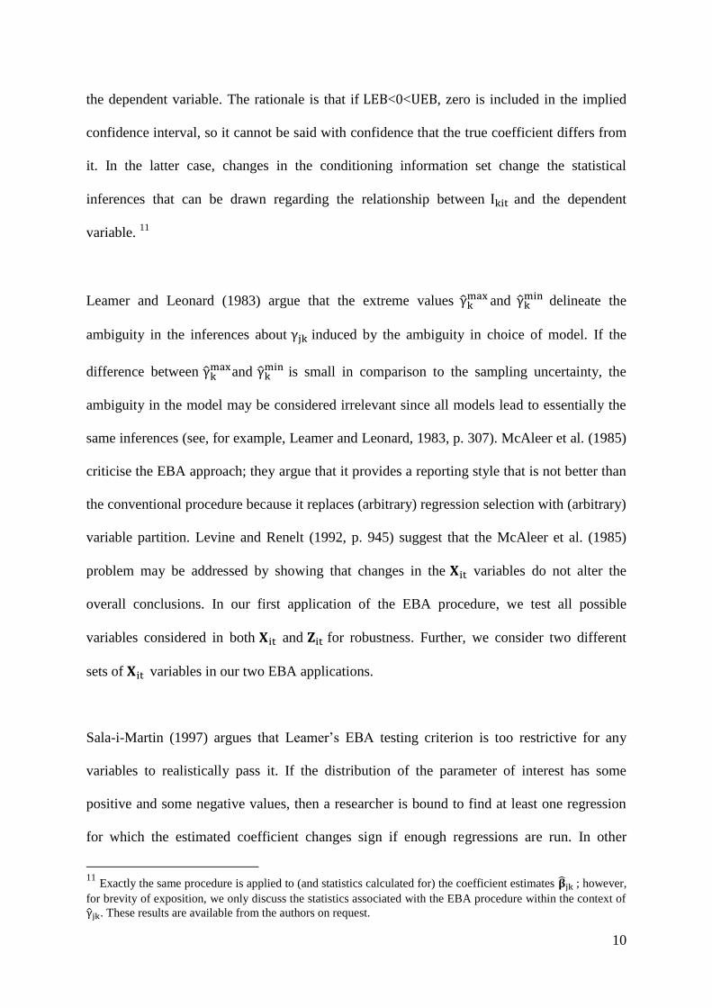
specification process in order to avoid the perception of data mining or selective reporting of

results. There are M possible combinations for each of the k=1,2,…,K variables of interest,

giving a total of possible regressions. Finally, is an error term. The aim is to

investigate the effects on the statistical significance of , the coefficient on the kth

variable

of interest, when varying the combinations of three variables included in .

10

The ( ) estimated coefficients for each , , and , , are recorded. The

standard deviation of these coefficient estimates is calculated for the each and is

denoted as . The highest and lowest values of are represented by and

,

respectively. The “extreme bounds" are defined as in Leamer (1983), where the lower

extreme bound ( ) and upper extreme bound ( ) are calculated using:

(3)

(4)

Clearly, LEB<UEB and these values form a range within which the true coefficient lies.

According to Leamer (1983, 1985), the variable is a “robust” determinant of the

dependent variable if the extreme bounds ( and ) are of the same sign; whereas, if

and have different signs, is described as having a “fragile” relationship with

10

To give the results more credibility, Levine and Renelt (1992) restrict their EBA in three ways. First, they use

three variables only, hence restricting the number of explanatory variables in each equation. Second, they

choose a small pool of variables from which the three variables are chosen. Third, for every variable of

interest, they restrict the pool of variables from which the variables are chosen by excluding variables that, a

priori, might measure the same phenomenon (ensuring that there are no close substitutes). They argue that these

restrictions make it more difficult to endogenously obtain fragile results. We also apply the first and third of

these restrictions, however, we do not apply the second because we believe that the large pool of economic and

geopolitical variables, , that we draw from, is a strength of our paper.

10

the dependent variable. The rationale is that if <0< , zero is included in the implied

confidence interval, so it cannot be said with confidence that the true coefficient differs from

it. In the latter case, changes in the conditioning information set change the statistical

inferences that can be drawn regarding the relationship between and the dependent

variable. 11

Leamer and Leonard (1983) argue that the extreme values and

delineate the

ambiguity in the inferences about induced by the ambiguity in choice of model. If the

difference between and

is small in comparison to the sampling uncertainty, the

ambiguity in the model may be considered irrelevant since all models lead to essentially the

same inferences (see, for example, Leamer and Leonard, 1983, p. 307). McAleer et al. (1985)

criticise the EBA approach; they argue that it provides a reporting style that is not better than

the conventional procedure because it replaces (arbitrary) regression selection with (arbitrary)

variable partition. Levine and Renelt (1992, p. 945) suggest that the McAleer et al. (1985)

problem may be addressed by showing that changes in the variables do not alter the

overall conclusions. In our first application of the EBA procedure, we test all possible

variables considered in both and for robustness. Further, we consider two different

sets of variables in our two EBA applications.

Sala-i-Martin (1997) argues that Leamer’s EBA testing criterion is too restrictive for any

variables to realistically pass it. If the distribution of the parameter of interest has some

positive and some negative values, then a researcher is bound to find at least one regression

for which the estimated coefficient changes sign if enough regressions are run. In other

11

Exactly the same procedure is applied to (and statistics calculated for) the coefficient estimates ; however,

for brevity of exposition, we only discuss the statistics associated with the EBA procedure within the context of

. These results are available from the authors on request.

11

words, under this test a variable is considered “fragile” if only one regression out of many

thousands causes a change in the sign of a coefficient. He noted that if one keeps trying

different combinations of control variables included in the samples drawn within some error

from the true population, then one is virtually guaranteed to find a model for which the

coefficient of interest becomes insignificant or even changes sign. As a result, one may

conclude that no variables are robust or that the test of robustness is extremely difficult to

pass.

Sala-i-Martin (1997) proposes an alternative form of EBA to determine a variable’s

robustness, derived from Leamer’s (1983) methodology and using essentially the same model

as specified in equation (2). However, his approach differs in the way the extreme bounds of

are calculated. His determination of robustness is based on the fraction of the Cumulative

Density Function (CDF) of that lies to the right of zero (using the entire distribution of the

estimated coefficients). If this fraction is sufficiently large (small) for a positive (negative)

relationship, is regarded as robust. Sala-i-Martin argues that if at least 90% of the CDF

for lies on either side of zero, it is probably safe to conclude that is robust. Sala-i-

Martin’s criterion is more lenient than Leamer’s and increases the likelihood that a variable is

robust. This discussion illustrates that there is no uniform definition of robustness.12

We

regard a variable as robust if it passes either Leamer’s or Sala-i-Martin’s EBA criteria.

We apply two variants of Sala-i-Martin’s (1997) EBA, being the normal and non-normal

12

This is explicitly recognised in Florax et al. (2002), who consider a range of definitions of robustness. They

analyse the sign, size and significance of regression results. This analysis extends Levine and Renelt and Sala-i-

Martin’s work by not only considering a wide range of robustness definitions but also explicitly analysing the

robustness of the sizes of the estimated effects. The robustness criteria adopted by Levine and Renelt and Sala-i-

Martin focus mainly on statistical significance. Whether the estimated effect sizes are robust to changes in the

conditioning set of variables is hardly addressed. We refer here to McCloskey and Ziliak (1996), for a pervasive

critique on this practice in economics. To assess robustness along this dimension, Florax et al. (2002) extend the

definition of robustness by requiring that the average estimated effect sizes conditional upon the inclusion of a

particular variable are within predetermined bounds from the overall average estimated effect size.

12

CDF methods. We discuss both below.

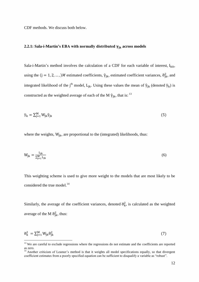
2.2.1: Sala-i-Martin’s EBA with normally distributed across models

Sala-i-Martin’s method involves the calculation of a CDF for each variable of interest, ,

using the ( ) estimated coefficients, , estimated coefficient variances, , and

integrated likelihood of the jth

model, . Using these values the mean of (denoted ) is

constructed as the weighted average of each of the M , that is: 13

∑ (5)

where the weights, , are proportional to the (integrated) likelihoods, thus:

∑

(6)

This weighting scheme is used to give more weight to the models that are most likely to be

considered the true model.14

Similarly, the average of the coefficient variances, denoted , is calculated as the weighted

average of the M , thus:

∑

(7)

13

We are careful to exclude regressions where the regressions do not estimate and the coefficients are reported

as zero. 14

Another criticism of Leamer’s method is that it weights all model specifications equally, so that divergent

coefficient estimates from a poorly specified equation can be sufficient to disqualify a variable as “robust”.

13

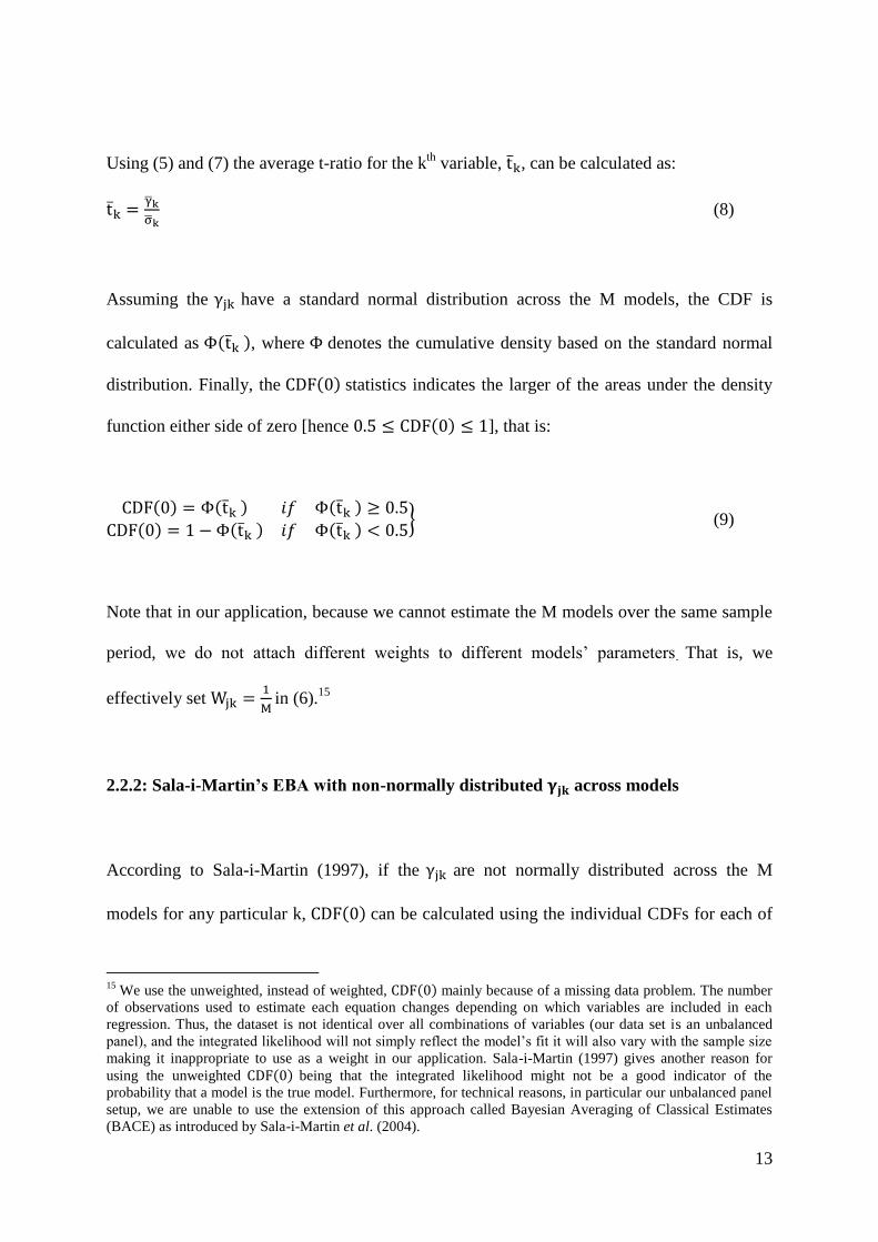
Using (5) and (7) the average t-ratio for the kth

variable, , can be calculated as:

(8)

Assuming the have a standard normal distribution across the M models, the CDF is

calculated as ( ), where denotes the cumulative density based on the standard normal

distribution. Finally, the ( ) statistics indicates the larger of the areas under the density

function either side of zero [hence ( ) ], that is:

( ) ( ) ( )

( ) ( ) ( ) } (9)

Note that in our application, because we cannot estimate the M models over the same sample

period, we do not attach different weights to different models’ parameters. That is, we

effectively set

in (6).

15

2.2.2: Sala-i-Martin’s EBA with non-normally distributed across models

According to Sala-i-Martin (1997), if the are not normally distributed across the M

models for any particular k, ( ) can be calculated using the individual CDFs for each of

15

We use the unweighted, instead of weighted, ( ) mainly because of a missing data problem. The number

of observations used to estimate each equation changes depending on which variables are included in each

regression. Thus, the dataset is not identical over all combinations of variables (our data set is an unbalanced

panel), and the integrated likelihood will not simply reflect the model’s fit it will also vary with the sample size

making it inappropriate to use as a weight in our application. Sala-i-Martin (1997) gives another reason for

using the unweighted ( ) being that the integrated likelihood might not be a good indicator of the

probability that a model is the true model. Furthermore, for technical reasons, in particular our unbalanced panel

setup, we are unable to use the extension of this approach called Bayesian Averaging of Classical Estimates

(BACE) as introduced by Sala-i-Martin et al. (2004).

14

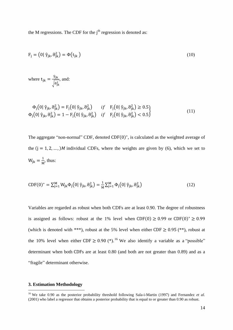
the M regressions. The CDF for the jth

regression is denoted as:

( | ) ( ) (10)

where

√

, and:

( | ) ( |

) ( | )

( | ) ( |

) ( | )

} (11)

The aggregate “non-normal” CDF, denoted ( ) , is calculated as the weighted average of

the ( ) individual CDFs, where the weights are given by (6), which we set to

, thus:

( ) ∑ ( | )

∑ ( |

) (12)

Variables are regarded as robust when both CDFs are at least 0.90. The degree of robustness

is assigned as follows: robust at the 1% level when ( ) or ( )

(which is denoted with ***), robust at the 5% level when either (**), robust at

the 10% level when either (*).16

We also identify a variable as a “possible”

determinant when both s are at least 0.80 (and both are not greater than 0.89) and as a

“fragile” determinant otherwise.

3. Estimation Methodology

16

We take 0.90 as the posterior probability threshold following Sala-i-Martin (1997) and Fernandez et al.

(2001) who label a regressor that obtains a posterior probability that is equal to or greater than 0.90 as robust.

15

3.1. Data

In order to assess the determinants of FDI, we have assembled a large panel dataset with an

extensive list of potential explanatory factors. These factors were chosen using theories of the

determinants of FDI and previous empirical studies on the determinants of FDI. 17

The

definitions and sources of the variables used are given in Table 1 and Table 2. Data were

constructed from a number of data sources, including World Development Indicators 2006

(denoted WDI in the tables). The political and institutional variables are obtained from the

International Country Risk Guide (ICRG) and we construct the geographical dummy

variables. Our sample is an unbalanced annual panel dataset consisting of 58 economic,

political and geographical variables for 168 economies over the period 1970–2006, which

gives a (maximum) total of 6048 observations. As far as we are aware no previous study of

FDI has covered such a long period with such a large number of economic, geographical and

political variables.

[Insert Table 1]

[Insert Table 2]

The sample period covered is determined by the availability of the data. The sample size

varies for different regressions estimated in the EBA procedure due the availability of data

being different for the different combinations of variables included in a particular regression.

17

See Chakrabarti (2001, Table 1) for a detailed discussion of empirical findings on the determinants of FDI.

Table 1 in his paper indicates how ambiguous the evidence is.

16

3.2. Estimation issues

Since the fixed-effects estimator does not assume that effects are uncorrelated with the error

term while the random-effects estimator does, it is far more likely that the strict exogeneity

assumption will be violated with the latter than the former method. Hence, the fixed-effects

estimator is more likely to ensure consistent estimates in our numerous EBA regressions than

the random-effects estimator and its use is therefore favoured a priori.18

For this reason our

first application of EBA that considers only economic determinants employs the fixed-effects

estimator in all regressions.

However, when political and geographical variables are added to the analysis, we can only

estimate the models using the random-effects estimator because some of these variables will

be perfectly collinear with the (cross-sectional) fixed effects. For example, our geographical

covariates include dummy variables for five different regions; these variables only vary

across sections and not through time – see Table 2 for the regions considered. Hence the

random-effects estimator is employed in our second application of EBA that incorporates

economic, geographical and political variables.

To obtain a satisfactory econometric model we have to consider the issue of endogeneity.

When explanatory variables are endogenous, ordinary least squares (OLS) gives biased and

inconsistent estimates of the causal effect of an explanatory variable on the dependent

variable. We identify three potential determinants as being the most likely to be

endogenously determined with FDI as the current account balance (CAB), GDP growth

18

Application of the Hausman test and F-test in initial modelling suggested the use of the fixed-effects estimator

when only time–variant (economic) variables are included as determinants.

17

(GDPG) and per-capita GDP (GDPP). 19

Temple (1999) argues that there exists a robust correlation between investment and growth

and empirically a number of studies have shown that causality runs from growth to

investment and vice versa. Hence FDI may determine growth. For example, FDI may affect

economic growth directly because it contributes to capital accumulation and the transfer of

new technologies to the recipient country. In addition, FDI enhances economic growth

indirectly where the direct transfer of technology augments the stock of knowledge in the

recipient country through labour training and skill acquisition, new management practices

and organizational arrangements (Blomstrom et al., 1994; Barro and Lee, 2001; and Sala-i-

Martin, 1996).

Mencinger (2008) highlights three indirect effects of FDI on the current account balance as

follows. First, if FDI increases capital formation without crowding out domestically financed

investment, it worsens the current account by the same amount. Second, if FDI crowds out

domestically financed investment, the effects depend on the reduction of domestically

financed investment; a part of FDI can be used to finance existing indebtedness of the

country. Third, if FDI implies acquisition of the existing assets in the host country, FDI

19

To consider the presence of endogeneity we apply the Wu-Hausman test. The Wu-Hausman tests are based

upon a fixed-effects estimated example regression of (

) on the 6 covariates CAB, GDPG, GDPP, OPEN,

INFL, TTRADE and the 3 residual series from the reduced form instrument equations for the 3 potentially

endogenous variables CAB, GDPG and GDPP. The reduced form instrument equations are fixed-effects

regressions of each of the 3 potentially endogenous variables on the 7 (presumed) weakly exogenous covariates

OPEN, INFL, TTRADE, CGD, RATIOT, GS and GCF. The results of these tests are available upon request.

The probability value for the Wu-Hausman F-statistic for testing the joint exclusion of the three residual series is

0.0822. This means that the three variables are jointly weakly exogenous at the 5% level although they are not

jointly weakly exogenous at the 10 % level. The 3 Wu-Hausman t-tests indicates that CAB is not weakly

exogenous (the t-ratio is –2.253) while GDPG (–0.413) and GDP (–0.604) are weakly exogenous. Hence, there

is some evidence that weak exogeneity is violated for all three variables jointly (at the 10% level) and CAB

individually. We are also concerned that our instrument equation for GDPG may be weak which may affect the

results from the Wu- Hausman test (the F-statistics of the fixed-effects instrument regressions are 14.418 for the

CAB equation, 279.070 for GDPG and 5.125 for GDPG which are all significant at the 5% level). Given that

there are reasons to believe that these three variables are potentially endogenous these example results suggest

that we should not assume that these variables are weakly exogenous.

18

provides a source of financing of the existing current account deficit.

We therefore treat CAB, GDPG and GDPP as endogenous in our EBA applications because

the costs of incorrectly treating exogenous variables as endogenous are much lower than

incorrectly assuming endogenous variables are exogenous. This means that these three

variables are excluded from and in all EBA applications and are only considered as

variables. Hence, the only inference that could be affected by endogeneity bias is when

these covariates are considered as the variable of interest.

4. Econometric Results

This section presents and discusses the results of our robustness analyses using EBA. The

empirical results are presented in two subsections. In section 4.1 we discuss the results of the

EBA applied only to economic variables whereas section 4.2 discusses the EBA application

involving economic, political and geographical variables.

4.1. EBA using only economic variables

The 30 potential economic determinants of FDI that we consider in our first EBA application

are listed in Table 1. The following three core variables, , that are always kept in the

equation are: openness (denoted Open), inflation (Infl), and tax on trade (Ttrade). These core

variables are chosen because they have been shown to be robustly linked to FDI in previous

empirical work (as well as in our initial experiments) and we do not expect them to be

endogenous. All of the remaining 27 economic determinants are considered as the variable of

interest, , however only 24 of these are included in because we are seeking to

19

minimise the impact of any endogeneity bias that the current account balance (CAB), GDP

growth (GDPG) and per-capita GDP (GDPP) variables may cause.20

Tables 3 to 6 summarise the results of our first EBA application. The first column reports the

variable of interest under consideration. For each variable four sets of EBA statistics are

reported: one set for the variable (reported in Table 6) and one set for each of the 3 core

variables: Open (Table 3), Infl (Table 4) and Ttrade (Table 5).21

The column headed “Obs”

gives the number of regressions estimated for each .22

This is below the maximum number

of possible regressions and this is mainly due to insufficient observations preventing the

estimation of some models. This causes some variation in the number of regressions run for

the different .

[Insert Table 3]

[Insert Table 4]

20

We note that in our first EBA application the variables in have pairwise correlation coefficients that are (in

all cases) below 0.5 in magnitude. This should limit the problem of multicollinearity which can adversely affect

conclusions regarding robustness. 21

In Tables 3 – 5 each core variable is tested for robustness with the test results specified in a disaggregated

form for each of the non-core variables. In contrast, Table 6 assess the robustness of the non-core variables of

interest, . 22

Assuming that all models contain the same number of variables in , p, the total possible number of

regressions for any particular is: ( )

( ) , where the ( ) arises because the variable is

removed from the set of variables in from which the various combinations of p=3 variables in are

taken. For all in a whole EBA application the total number of regression is . Because we exclude 3

potentially endogenous variables from this implies that ( ) for these 24 “non-endogenous”

variables’ applications of EBA. Hence, the number of regressions for each of these 24 variables is ( ( )

( ) ) and the total for all 24 variables is ( ) . Whereas, for the three

potentailly endogenous variables we only exclude the other 2 potentially endogenous variables from their EBA

applications, hence ( ) . Thus, for each potentially endogenous variable the number of estimated

regressions is ( ( )

( ) ) and so for all 3 of these variables the total is ( ) .

Hence, the maximum number of regressions estimated in the first EBA application is

( ) . Because some models do not estimate due to, for example, insufficient

observations, the actual number of estimated models in the EBA application is below this.

20

[Insert Table 5]

[Insert Table 6]

The column headed “AVG coeft” gives the variable’s coefficient averaged over the number

regressions (Obs) used in the EBA application. Also reported in the tables are the averaged

coefficient standard error (“AVG S.E.”) and absolute t-ratio (“AVG T”).23

The columns

headed and give Leamer’s lower and upper bounds, respectively.24

Sala-i-

Martin’s (1997) non-normal CDF [denoted ( ) ] and normal CDF [ ( )] statistics are

also reported in the tables.25

The final column (“robustness”) indicates whether a variable is

robust (and its degree of robustness), possibly robust or fragile, based upon Sala-i-Martin’s

criteria. For a variable to be robust it must have a CDF of at least 0.90 according to both

normal and non-normal criteria (the normal and non-normal CDF broadly yield the same

inference). Similarly a variable is a possible determinant if both CDF criteria are at least 0.80

(and the variable is not regarded as robust), otherwise the variable is said to be fragile.

The first inference we draw from Table 3 – 6 is that none of the 27 variables are robust

according to Leamer’s (1983) criterion because and have different signs in all

cases. This likely reflects the overly stringent nature of this criterion and we therefore do not

base our conclusions upon it.

23

Note that AVG T is not equivalent to (8). This is because (8) averages the numerator and denominator of the

t-ratio before applying the division whereas AVG T divides the numerator by the denominator first and then

averages the result. 24

These are calculated using (3) and (4). 25

These are calculated using (12) and (9).

21

However, variables are robust according to Sala-i-Martin’s (1997) CDF criteria. Table 3

indicates that the core variable, Open, is robust in 26 out of 27 sets of EBA results (the

exception is when Timeb is the variable of interest). This result is consistent with many

previous studies that found openness toward trade to be a significant determinant of FDI as it

provides funds for economic expansion (see Chakrabarti, 2001 and Moosa, 2006). In all 27

cases Open has an average coefficient sign (see the column headed “AVG coeft”) that is

positive which is consistent with theoretical expectations. In contrast, the Infl core variable is

robust in only one (Ratiot) of the 27 EBA sets – see Table 4. Infl is a “possible” determinant

for 3 variables of interest (Internet, Liquid and Timeb) because both of their CDFs are

between 0.80 and 0.89 and is a fragile determinant for the remaining 23 . The Ttrade core

variable is robust in only one (Cgd) of the 27 EBA sets and is a “possible” determinant for 3

variables (REX, TEL and UNEM), see Table 5. Hence, we consider this as strong evidence

against Ttrade and Infl being robust determinants of FDI.

From Table 6 we see that eight non-core variables are unambiguously robust determinants of

FDI according to Sala-i-Martin’s criteria because both of their CDFs exceed 0.90. These are

CAB, GDPG, GDPP, Hmtaxcor, FDIO, Ratiot, Ratios and GFE. Four variables, (Wgetogdpl,

GCF, TEL and Taxprofr) are considered “possible” determinants because both their CDFs are

at least 0.80 and do not exceed 0.89. All of the other variables in our first EBA application

are fragile. Comparing our findings with previous applications of EBA to FDI using EBA

(that considered far fewer potential determinants than we do) provides interesting insights.

Moosa (2006) found telephone mainlines to be robust whereas we find it to be fragile.

Further, Moosa found GDP growth and tertiary enrolments to be fragile while we find these

variables to be robust. Chakrabarti (2001) found openness and GDP to be robust as we do.

Hence, whilst previous studies provide some inferences that are consistent with our results

22

many are not consistent. We believe that our results are more reliable due to the greater

coverage of data, sample size and larger number of potential determinants considered.

We now discuss the variables that we find to be robust and “possible” determinants in more

detail. The robust Hmtaxcor variable combines the effects of corporate taxes on FDI with

very high levels of profitability and effects on marginal investments which determine the

volume of an existing capital stock. The effect of Hmtaxcor on FDI is expected to be negative

because a multinational corporation (MNC) will decide to invest where tax on marginal profit

is lower compared to alternative locations. As expected Hmtaxcor has a generally negative

sign (indicated by the “AVG coeft” statistic) as a higher Hmtaxcor implies a lower level of

after tax profits. Our results suggest that a host country with high corporate taxes will have a

robust negative effect on FDI.26

FDI outflows (FDIO) is another robust determinant of FDI inflows. Increased

competitiveness is one of the prime benefits that a developing country’s MNCs can derive

from their FDI outflow activities. We find that FDIO generally has a positive impact on FDI

which is consistent with theoretical expectations.

The tertiary enrolment ratio (Ratiot) and secondary enrolment ratio (Ratios) are both found to

be robust determinants of FDI and represent those factors that capture the impact of labor

productivity and wage rates on FDI. Theory suggests a clear-cut sign for these coefficients

(positive), as human capital is generally considered a prime driver of productivity and

investment; FDI should be no exception here. Indeed, we find that both Ratios and Ratiot

26

Recently Becker et al (2012) stated that the quantity of FDI is affected if corporate taxes reduce the

equilibrium stock of foreign capital in a given country, while quality effects arise if taxes decrease the extent to

which investment contributes to the corporate tax base and capital intensity of production.

23

have generally positive coefficients which are consistent with theoretical expectations and

implies that education attracts vertical FDI.27

Government expenditure as a proportion of GDP (GFE) is robust and has, on average, a

negative sign, as is theoretically expected. The reason for this negative relationship as

suggested by Onyeiwu (2003) and Filipovic (2005) is that a large size of the government may

create opportunities for misuse of funds by government officials, crowd-out private

investment (including FDI) and creates an elaborate and complex bureaucratic structure that

makes the investment climate unattractive to FDI as it may increase future taxation.

Theory suggests that an increase in GDPG and GDPP leads to an increase in FDI. For

example, higher GDPP indicates greater aggregate income and or more companies, and

therefore a higher ability to invest abroad, while smaller GDPP in host country implies

limited market size and a consequent desire by companies to expand their operations overseas

in order to gain market share. We find that both GDP variables are robust and have generally

positive coefficient signs, which is consistent with theoretical expectations.

Next, we find that the current account balance (CAB) affects FDI with an overall negative

sign. This is consistent with theory, as from National Income Accounting we have CA=S-I, in

obvious notation.28

Thus, if incoming FDI augments total domestic investment and does not

27

The hypothesis that human capital in host countries is a determinant of FDI has been embodied in the

theoretical literature. For example, Lucas (1993) conjectures that lack of human capital discouraged foreign

investment in less-developed countries. Zhang and Markusen (1999) present a model where the availability of

skilled labor in the host country is a direct requirement of MNCs and affects the volume of FDI inflows.

Dunning (1988) maintains that the skill and education level of labor can influence both the volume of FDI

inflows and the activities that MNCs undertake in a country. Noorbakhsh et al. (2001) concluded that human

capital plays an increasingly important role over time in attracting FDI. Further, the educational level and skills

of workers affect their productivity. Indeed the level of human capital increases the ability of workers to learn

and adopt new technologies faster and more efficiently and thus boost up the productivity of the sector. 28

To see this, we can start from basics : GNP=C+I+G+CA, therefore GNP-C-G=I+CA, therefore CA=S-I,

where S is national saving (private + public).

24

simply crowd out indigenous investment one-for-one (an extreme outcome), I increases with

FDI. If the marginal propensity to save is between zero and one, as is plausible, then S will

rise but by a smaller amount. Thus, CA will fall.

We now discuss the 4 determinants (Gcf, TEL, Wgetogdpl and Taxprofr) that we find to be

“possibly” robust in more detail. Gross Fixed Capital Formation (Gcf) is total domestic

investment, so, following the above reasoning, there will be a positive relation with FDI

except in the extreme and unlikely situation where foreign investment entirely crowds out the

indigenous one. We find a generally positive relationship which is consistent with this

theoretical expectation. The number of telephones per 1000 inhabitants (TEL) is a standard

proxy of infrastructure development in the literature. An established and advanced

infrastructure facility of the host country provides a great platform for investment and leads

to greater FDI (a positive coefficient is expected). Our results indicate a generally positive

coefficient for this variable which is consistent with theoretical expectations. However, the

wage-GDP ratio (Wgetogdpl) has, on average, a positive coefficient which is theoretically

unexpected. Having said this, Charkrabarti (2001) argues that using the wage to proxy labour

costs as a determinant of FDI is contentious. There is no unanimity in the previous studies

regarding the role of wages in attracting FDI. ODI (1997) suggests that empirical research

has found the wage to be statistically significant for foreign investment in labour-intensive

industries and for export–oriented subsidiaries. However, when the cost of labour varies little

from one country to another, it is the skills of the labour force that are expected to have an

impact on decisions about FDI location.

Tax on profit (Taxprofr) is our last “possible” economic determinant of FDI. One potential

explanation is linked to whether the parent multinational company (MNC) is export oriented,

25

in which case it may view taxes as highly influential in its investment decisions, while a retail

MNC seeking specific advantages from the domestic market may prioritise factors other than

tax. Our finding is in line with Morisset’s (2003) statement that, “the effectiveness of tax

incentives is likely to vary depending on a firm’s activity and its motivations for investing

abroad”. Another possible justification of Taxprofr being a “possible” determinant is an

increase in profit shifting opportunities (or costs) from one host country to another is a

strategy of MNCs to reduce the tax rate. Genschel (2001) suggests that MNCs that undertake

production activities face in general high transactions cost and profit-shifting is almost

prohibitive so that locational advantages such as tax on profit become an important

determinant. However MNCs that invest in services, finance and R&D face relatively low

costs when shifting profits and hence real activity plays only a small role in determining

investment decisions. We find that Taxprofr typically has a negative coefficient which is

consistent with our theoretical expectations.

Of these 9 robust, and 4 possibly robust, variables (Open, GFE, FDIO, Tel, Ratios, Ratiot,

Cab, GDPG, GDPP, Hmtaxcor, Taxprofr, Gcf, Wgetogdpl), 12 have theoretically expected

(average) coefficient signs. However, the possibly robust Wgetogdpl variable has a

theoretically unexpected average coefficient sign. However, we treat the finding of

robustness for the three potentially endogenous variables Cab, GDPG and GDPP with caution

and hesitate to conclude that our results offer strong support for their robustness.

4.2. EBA using economic, geographical and political variables

In our second EBA application we include Open, Gfe and Ratios as our core variables

following the results of our first EBA. Open is chosen because it is the only core variable

26

from our first EBA application that is robust. Since the other two core variables (Infl and

Ttrade) are not robust in our first EBA application we seek two different core variables for

our second EBA application. The criteria used to select these two core variables are those

robust variables with an average coefficient sign that is consistent with theoretical

expectations in the first EBA application that have the highest value for ( ) and are not

one of the 3 potentially endogenous variables. The 3 variables with the highest values for

( ) are Gfe ( ( ) ), Ratios (0.95) and Cab (0.95). Since we regard Cab as

potentially endogenous we select the other 2 as core variables, along with Open, to be

employed in our second EBA application. Our first EBA application arguably suggests that

these are the most likely economic variables to be robust.

We add 28 geographical and political variables (Table 2) to the economic variables to be

considered in the second EBA application allowing us to test the robustness of an extended

set of variables. The geopolitical variables are not included in the core set of variables, , or

the set of three variables (to help avoid multicollinearity), however, they are all

considered (in turn) as the variable of interest, . All of the economic variables (except the

3 core variables) are considered (in turn) as and in (except for the potentially

endogenous variables, Cab, GDPG and GDPP, and the 3 core variables).29

In this second application, based on the institutional quality hypothesis by North (1990) that

highlight the relationship between FDI and political institutions we are trying to determine

29

For the EBA involving the 24 (not potentially endogenous) economic and 28 geopolitical variables the

(maximum) number of estimated models (with K=24 variables in ) for each variable of interest is (

( )

( ) ) , giving a total of {[(24+28) * 1771]=} 92092 regressions. For the 3 endogenous variables

the (maximum) total number of regressions is ( ) – see calculations above. Hence, the

maximum number of regressions estimated in this second EBA application is 98164. Thus, in the two EBA

applications, we estimated (98164+48576=) 146740 models.

27

whether country specific institutions (such as democracy, corruption, bureaucracy and

conflict), cultural factors (languages) or geographical locations (number of boundaries, costal

location, abundance of natural resources, proximity to particular regions) can influence FDI.

Many geographical and political/institutional factors have been conclusively linked to

economic growth (see e.g. Durlauf et al., 2005) and remain active areas of research. The

results of our second EBA application are reported in Table 7 and for economic variables and

in Table 8 for geopolitical variables. As before, none of the 55 variables are robust according

to Leamer’s (1983) criterion because and have different signs in all cases; again,

due to the overly stringent nature of this criterion, we do not base our conclusions upon it.

According to both of Sala-i-Martin’s (1997) CDF criteria, only 10 of the 28 geopolitical

variables are considered as robust determinants of FDI as both of their CDFs are at least 0.90.

These include the dummies for: countries in the South Asia region (SA), countries in the East

Asia and pacific region (EAP), countries with more than 3 boundaries (GTBUN), countries

that are not land-locked (landunlocked), Spanish (SPN) and Arabic speaking countries (ARB)

as well as nations with greater democratic accountability (DEMO). These seven determinants

are all generally positively correlated with FDI inflows. The other three robust geopolitical

variables are dummies for: countries experiencing low international and internal conflict

(conflictint) and economies with an abundance of the natural resources: oil (oildummy) and

gas (gasdummy).

[Insert Table 7]

The results indicate regional effects such that the South Asia and EAP regions receive

relatively high FDI after controlling for other factors. This is consistent with the empirical

28

evidence that South Asia countries received the largest share of FDI. Vial (2002) suggested

many reasons behind the increase of FDI to this particular region such as the change in the

political climate and the receptivity towards foreign capital. Further, the process of reforms

through which these countries have gone through and the new business climate in natural

resource sectors may also explain the increase in FDI in this region. Other possible

explanation is the geographic proximity of this region to China.30

SA and EAP regions have captured most of the increased investment. These regions include

economies which offer the best climate for doing business. The development experiences of

EAP countries such China, Singapore, Hong Kong and Taiwan emerged as locations offering

distinct hubs of labour-intensive exports owing to low labour costs.

Democracy can increase FDI inflows because they provide checks and balances on elected

officials, and this in turn reduces arbitrary government intervention, increases information

and transparency, lowers the risk of policy reversal and strengthens property right protection

(Jensen, 2008 and Li, 2009).31

This is consistent with our finding of DEMO as a robust

determinant with a generally positive coefficient sign.

The Internal and external conflict variable (conflictint) is found to be robust in determining

FDI with a generally negative coefficient sign. This is consistent with a priori expectations as

less conflict reduces incertitude amongst potential investors, which raises FDI. As Sacks

(2003) explains, an investor’s mindset is to invest in a venture if the payoff is high enough

30

Our results also show that the SSA and MENA dummies are fragile determinants of FDI. One of the plausible

explanations is the weak institutions in these regions. 31

However, Asiedu (2011) finds that democracy attracts FDI in countries where the share of natural resources in

total exports is low, but has a negative effect on FDI in countries where exports are dominated by natural

resources. This statement may to some extent explain why we did not find the SSA and Mena regions as robust

determinants of FDI (the countries in these regions have weak democracy and their exports are dominated by

natural resources).

29

given the risk. Hence, an increase in institutional quality (as indicated by greater democracy

and lower conflict) would increase FDI inflow.

Our results also suggest that language can be considered as a dynamic instrument to attract

FDI. We found that countries that speak Arabic and Spanish increase FDI ceteris paribus.

The main possible explanation is that the transaction costs of those two languages are higher

than, for example, French and English (dummies representing countries speaking these latter

two languages are found to be fragile). Hence, these results are consistent with prior beliefs.

Being a landlocked country is disadvantageous because the country has no direct access to

seaborne trade. Landlocked developing countries have significantly higher costs of

international cargo transportation compared to coastal developing countries and more

freedom to choose their trading partners. It has been found in growth empirics that economic

growth is negatively affected if a country is landlocked (Easterly and Levine, 2001).

Consistent with that, we find that coastal countries tend to attract more FDI.32

This is

consistent with our finding that the dummy variable “landunlocked”, measuring countries that

are not landlocked, is a robust determinant with a generally positive sign. We also find that

countries with more than 3 boundaries attract more FDI than those with fewer boundaries

given the robust and generally positive coefficient. This is also in the spirit of the previous

finding (the landlocked feature): a country with more neighbours has more freedom to trade.

Hence, there are better prospects for incoming FDI. While “landlockdeness” has been

emphasised in the past as a factor affecting growth and FDI, the finding that the numbers of

borders affects FDI is, we believe, novel.

32

As an interesting aside, the surface area of a country is not a robust determinant of FDI.

30

Natural resource abundance in the form of oil and gas (oildummy and gasdummy,

respectively) are found to be robust determinants of FDI with generally negative coefficient

signs. Our finding is consistent with the results of Sachs and Warner (1996) who find that the

natural resource abundance induces a kind of ‘Dutch disease’ that affects growth negatively.

Furthermore, as has been suggested by Tietenburg (2006), large rents in the natural resource

sector crowd out investment in other sectors, and therefore possibly inward FDI. This

reasoning will of course not apply to specifically resource-seeking firms, which would

naturally be attracted by resource abundance; this would explain the inflows of FDI into the

Arab Gulf and African countries.

Finally, rule of law, parliamentary regime and the Europe and central Asia dummy variables

are found to be possible determinants of FDI while all other geopolitical variables exert only

a fragile influence on FDI. As mentioned, political and other institutions are a vibrant area of

research in growth theory and empirics (see e.g. Easterly et al., 2004; Glaeser et al., 2004;

and the review of Durlauf et al., 2005).

From Table 8 we see that eight non-core economic variables are robust determinants of FDI

according to Sala-i-Martin’s criteria. These are CAB, GDPG, GDPP, CGD, FDIO,

INTERNET, RATIOT and TEL.

[Insert Table 8]

The findings in Table 8 are similar to those in Table 6 in that FDIO, RATIOT, CAB, GDPG

and GDPP are found to be robust in both of our EBA applications. The average coefficient

signs are the same in Table 8 and Table 6 except for RATIOT which has a generally negative

31

coefficient sign in Table 8; this is rather counterintuitive. This change in coefficient sign

between the two EBA applications may be due to RATIOS being a core variable in the

second application and not the first. This broadly confirms the robustness of these results.

Table 8 suggests three additional robust variables, which are central government debt (CGD),

internet use (internet) and telephone mainline use (TEL). CGD appears as robust with a

generally negative coefficient: this is expected, as debt may have a number of adverse

consequences, such as inducing higher interest rates and raising default risk. The latter two

capture communication facilities. As expected an increase in internet and telephone use

increases FDI inflows as indicated by the generally positive coefficient signs for these

variables.

Four variables, (LIQUID, POPTL, GCF and TAXPROFR) are considered “possible”

determinants of FDI. The last two variables (GCF and TAXPROFR) were also found to be

“possible” determinants of FDI in our first EBA application indicating some further

consistency of results. All of the other variables in our second EBA application are fragile.

Overall, our results in Table 7 and 8 are in accordance with the literature, and support the

hypotheses that market size and market potential, human capital and communication facilities

as well as the availability of natural resources robustly determine FDI inflows. However, we

note that 37 of the 55 variables considered in our second EBA application are not robust. In

addition, we are cautious in concluding that the 3 potentially endogenous variables (GDPP,

GDPG and CAB) are robust determinants of FDI.

5. Conclusion

32

We investigate the determinants of FDI using an unbalanced panel dataset covering 168

countries over the period 1970 to 2006. We consider 58 economic, geographical and political

variables that have been previously proposed as determinants of FDI using EBA to address

the issue of model uncertainty. As far as we are aware this is the most variables that have

been considered using the largest coverage of data in any EBA application of the

determinants of FDI. Our EBA application to FDI extends previous work in its use of a large

unbalanced panel data set instead of just cross-sectional data which the majority of previous

analyses of FDI employ. Further, we consider a larger number of economic, political and

geographical variables than has been previously used in one empirical investigation in the

literature. We particularly emphasize the novelty of our use of political and geographical

factors. In these respects we believe our work significantly extends the existing literature that

seeks to understand the determinants of FDI.

We find that the Sala-i-Martin (1997) EBA approach is more ‘permissive’ than the Leamer

(1983) method. This is because no variables are found to be robust using the Leamer method,

whereas robust determinants can be identified using Sala-i-Martin’s approach. This confirms

the conclusions of the previous literature that the Leamer criterion is likely to be too strict to

usefully uncover the determinants of any particular variable. In contrast, Sala-i-Martin’s

approach can discern those determinants that are robust and those that are not.

In our first EBA application that only considers economic determinants of FDI we find that

the following six variables (excluding the 3 potentially endogenous covariates) have a robust

relationship (with average coefficient signs that are consistent with theoretical expectations)

according to both of Sala-i-Martin’s CDF criteria: Open, FDIO, GFE, Hmtaxcor, Ratiot and

Ratios. Based upon this we use Open, GFE and Ratios as the core variables in our second

33

EBA application that considers both economic and geopolitical determinants of FDI.

According to both of Sala-i-Martin’s (1997) CDF criteria our second EBA application reveals

that 18 of the 55 (non-core) variables are robust determinants of FDI. There are ten robust

geopolitical determinants that suggest the following relations with inward FDI. Countries

located in South Asia, East Asia and the pacific region, that have more than 3 boundaries,

that are not land-locked, that are Spanish or Arabic speaking, that have greater democratic

accountability and that experience less conflict attract more FDI. These results are consistent

with theoretical expectations and Globerman and Shapiro (2002) who concluded that

democratic governance as well as a reasonable level of peace and order and infrastructure are

perquisites for greater FDI inflows. Additionally, we re-affirm the Sachs and Warner (1996)

findings that natural resource abundance induces a “Dutch disease”; they explored the effect

for growth, while here we find that this affects negatively incoming FDI.

The three core economic variables used in our second EBA application were not tested for

robustness. Nevertheless, these three variables – trade (openness), government expenditure

and human capital (secondary enrolment rates) – are presented as robust determinants of FDI.

Excluding the three potentially endogenous variables there are five robust (non-core)

economic determinants of inward FDI identified by our second EBA application. Notably

RATIOT is robust and has a generally negative coefficient which means that FDI tends to be

horizontal rather than vertical. Indeed, the finding that tertiary enrolment rates are robust in

the second EBA is consistent with secondary enrolment rates being robust in our first EBA.

However, RATIOT had a robust and generally positive coefficient in the first EBA

application and a robust and negative average coefficient in the second. This change in

34

coefficient sign between the two EBA applications may be due to RATIOS being a core

variable in the second application and not the first. The 4 economic variables, FDIO,

INTERNET, TEL and CGD are robust and have average coefficient signs that are consistent

with theoretical expectations.

Our study has important implications for policies aimed at promoting FDI and, therefore,

economic development. For example, countries that reinforce infrastructure facilities,

liberalise local and global investment policy and maintain macroeconomic and political

stability will improve inward FDI performance and become an attractive destination for

foreign investors.

Thus, open, ratios and ratiot are policy variables as they can be directly influenced by policy

makers in the short run, for example via changes in tax, public R&D expenditures, or bilateral

investment treaties etc. At the same time market size and political risk are ‘intervention

variables’ which can only be indirectly influenced by policy makers and/or changed in the

medium to long run. These policies should contribute to closing the gap between actual and

potential FDI.

In addition to our broader coverage of determinants and larger dataset we propose three

possible explanations regarding the differences between our results and previous results.

First, it is possible that foreign investment is attracted by a variety of determinants, a few

being predominant (such as openness, government spending and human capital ) and other

less relevant. Therefore, different sets of determinants are sufficient to attract FDI as long as

oppeness and human capital exists in the particular country. Second, the FDI performance

may be driven by specific determinants over a particular period reflecting strengths (such as

35

natural resources and good institutions) and weaknesses (for example, being in the early stage

of economic development compared with more mature economies) of each country relative to

the endowment in those determinants. Third, for a given sector, the production of this sector

may be of different range or quality across countries (luxury and low-range products) and

hence, investment in that sector may be responsive to different FDI determinants relative to

the range.

The econometric approach presented in this paper attempts to measure the influence on FDI

of not only economic factors that economists have traditionally considered, but also

geopolitical variables measuring political instability, government efficiency, geographic

closeness and cultural similarity. By using this extended set of varaibles we hope to provide a

more complete picture of the interaction of local and global forces that impact decisions to

invest abroad.

Our results suggest that economic institutions matter in attracting FDI because they shape and

influence investments in physical and human capital technology and the organization of

production. However, geopolitical variables also matter, especially for less developed

countries. Poor political institutions lead to poor infrastructure, low expected profitability and

less FDI.

References

Asiedu, E. and D. Lien, (2011). “Democracy, FDI and natural resources”, Journal of

International Economics, 99-111.

Barro, R. and J.-W. Lee, (2001). “Schooling Quality in a Cross-Section of Countries,”

Economica, 38, 465-488.

Becker, J. C., Fuest, C. and N. Riedel (2012). “Corporate tax effects on the quality and

quantity of FDI”, European Economic Review, 56 (8), 1495-1511.

36

Beugelsdijk S., H. L. F. de Groot and A. B.T.M. van Schaik, (2004). “Trust and economic

growth: a robustness analysis”, Oxford Economic Papers, 56, 118–134.

Blomström, M., R. E. Lipsey, and M. Zejan (1994). “What explains developing country

growth”, NBER Working Paper No. 4132.

Chakrabarti, A., (2001). “The determinants of foreign direct investment: sensitivity analyses

of cross–country regressions”, Kyklos, 54, 89-114.

Dunning, J. H. (1988). “The eclectic paradigm of international production: A restatement and

some possible extensions”. Journal of International Business Studies, 19 (1), 1–32.

Durlauf, S., P.A. Johnson and J.R.W. Temple (2005). “Growth Econometrics”, Chapter 8 in:

Aghion, P. and S. Durlauf (eds.) “Handbook of Economic Growth”, Amsterdam: North-

Holland.

Easterly, W. and R. Levine (2001). “It’s Not Factor Accumulation: Stylized Facts and

Growth Models” , World Bank Economic Review, 15, 177-219.

Easterly, W., R. Levine, and D. Roodma (2004). "Aid, Policies, and Growth: Comment",

American Economic Review, 94, 3, 774–780.

Fernandez, C., E. Ley, and M.F.J. Steel (2001). “Model uncertainty in cross-country growth

regressions”, Journal of Applied Econometrics, 16, 563-576.

Filipovic, A. (2005). “Impact of privatization on economic Growth”, Issues in Political

Economy, 14, 1-20.

Florax, R.J.G.M., H.L.F. de Groot and R. Heijungs (2002). “The Empirical Economic

Growth Literature: Robustness, Significance and Size”, Tinbergen Discussion Paper, TI

2002- 040/3, Amsterdam-Rotterdam.

Gassebner, M., M. J. Lamla and J. Vreeland (2012). “Extreme bounds of democracy”,

Journal of Conflict Resolution, forthcoming.

Genschel, P. (2001). “ Globalization, Tax Competition, and the Fiscal Viability of the

Welfare State”, MPIFG, Working paper01/1, Cologne.

Gilbert, C. L. (1986). “Professor Hendry’s econometric methodology”, Oxford Bulletin of

Economics and Statistics, 48, 283-307.

Glaeser, E.L., R. La Porta, F. Lopez-de-Silanes and A. Shleifer (2004): “Do Institutions

Cause Growth?” , Journal of Economic Growth, 9, 3, 271-303.

Globerman, S. and D. Shapiro (2002). “Global Foreign Direct Investment Flows: The role of

Governance Infrastructure”, World Development, 30, 11, 1899-1919.

Hussain, M. and O.S. Brookins (2001). “On the determinants of National Saving: An extreme

Bounds Analysis”, Weltwirtschftliches Archiv, 137, 151-174.

37

Hendry, D. and H. M., Krolzig (2004). “We Ran One Regression”, Oxford Bulletin of

Economics and Statistics, 66, 5, 799-810.

Hoover, K. D., and Perez, S. J. (2004). “Truth and robustness in cross-country growth

regressions”, Oxford Bulletin of Economics and Statistics, 66, 5, 765–798.

ICRG, various years, International Country Risk Guide Annual, PRS Group.

Jensen, N. M. (2008). “Political Risk, Democratic Institutions and Foreign Direct

Investment”, Journal of Politics, 70, 4, 1040-1052.

Leamer, E.E. (1983). “Sensitivity analysis would help”, American Economic Review, 75,

308-313.

Leamer, E.E. (1985). “Let’s take the con out of econometrics”, American Economic Review,

73, 31-43.

Leamer, E.E. and H. Leonard (1983). “Reporting the fragility of regression estimates”.

Review of Economics and Statistics 65, 306-17.

Leon-Gonzalez, R. and D. Montolio (2004). “Growth, Convergence and Public Investment: A

Bayesian Model Averaging Approach ”, Applied Economics, 36, 1925-1936.

Levine, R. (2003). “More on Finance and Growth: More Finance, More Growth?” Federal

Reserve Bank of St , Louis Review, 85, 4.

Levine, R., N. Loayza and T. Beck (2000). “Financial Intermediation and Growth :Causality

and Causes.”Journal of Monetary Economics, Vol. 46:31-77.

Levine, R. and D. Renelt (1992). ‘A sensitivity analysis of cross-country growth regressions,

American Economic Review, 82, 942–63.

Li, Q. (2009). “Democracy, autocracy, and expropriation of foreign direct investment”,

Comparative political Studies, 42, 8,1098-1127.

Lucas, R.E. (1993). “On the Determinants of Foreign Direct Investment: Evidence from East

and Southeast Asia", World Development, 21, 3, 391-406.

McAleer, M., A. Pagan and P.A. Volker (1985). “What will take the con out of

econometrics?” American Economic Review, 75, 293–307.

McCloskey, D. N. and S. T. Ziliak (1996). “The Standard Error of Regressions”, Journal of

Economic Literature, 34, 97-114.

Mencinger, J. (2008). “The addiction with FDI and current account balance”, International

Centre for Economic Research, Working Paper No.16/2008.

Moosa, I.A. (2006). “The determinants of foreign direct investment: An extreme bounds

analysis”, Journal of Multinational Financial Management, 16, 199-211.

38

Moser,C. and J.E. Sturm (2001). “Explaining IMF lending decisions after the Cold War”,

Review of International Organisations, 6, 3, 307-340.

Morisset, J. (2003). “Using Tax Incentives to Attract FDI”, Viewpoint (World Bank), January

2003 (https://www.wbginvestmentclimate.org/uploads/taxincentivesforeigninvestment.pdf).

North, D.C. (1990). “Institutions, Institutional Change, and Economic Performance”,

Cambridge: Cambridge University Press.

Noorbakhsh, F. and A. Paloni (2001). “Human capital and FDI inflows to developing

countries: New empirical evidence”, World Development, 29, 9, 1593–1610.

ODI (1997), "Foreign Direct Investment Flows to Low-Income Countries: A Review of the

Evidence", http://www.odi.org.uk/publications/briefing/3_97.html.

Onyeiwu, S. (2003). “Analysis of FDI flows to developing countries:Is the MENA region

different?” Paper presented at ERF10th Annual Conference, Marrakech, Morocco, December

2003.

Sachs, J. and A. Warner (1996). “Natural Resource Abundance and Economic, Growth”,

Sachs, J. (2003). “Institutions Don’t Rule: Direct effects of geography on per capita

Income”, NBER Working Paper No. 9490.

Sala-i-Martin, X. (1996). “I Just Ran Four million Regressions”, NBER Working Paper No.

6252

Sala-i-Martin, X, (1997). “I Just Ran Two Million Regressions”, American Economic

Review, 87, 178-183.

Sala-i-Martin, X., G. Doppelhofer and R. Miller (2004). “Determinants of long term growth:

a Bayesian Averaging of Classical Estimates (BACE)”, American Economic Review, 94, 4,

813-835.

Sturm, J. and J. de Haan (2005). “Determinants of long–term Growth: New Results Applying

Robust Estimation and Extreme Bounds Analysis”, Empirical Economics, 30, 597 – 617.

Temple, J. (1999). “The New Growth Evidence”, Journal of Economic Literature, 37, 112-

156.

Temple, J. (2000). “Growth Regressions and What the Textbooks don’t Tell You”, Bulletin

Of Economic Research, 52, 3, 181-205.

Tietenberg, T. (2006) “Environmental and Natural Resources Economics”. Pearson (5th

ed.)

Vial, J. (2002). “Building institutions for a more competitive region” in Vial, J. and P.

Cornelius (eds.), The Latin American Competitiveness Report, 2001-2002.

39

Wooldridge, J. M. (2000). “Introductory Econometrics: A Modern Approach”, Cincinnati:

South-Western College Publishing.

World Bank (2006).World Development indicators. CD-rom. World Bank,Washington D.C

Zhang, K. and K. Markusen (1999). “Vertical multinationals and host-country

characteristics”, Journal of Development Economics, 59, 3, 233-252.

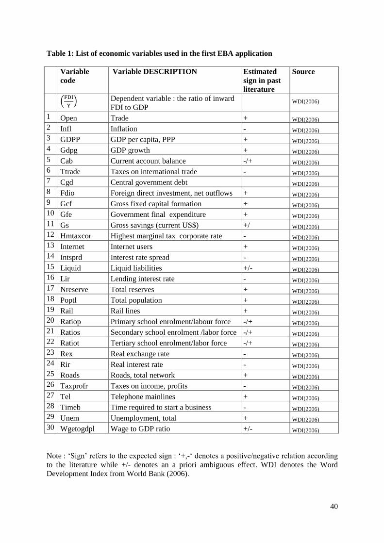
40

Table 1: List of economic variables used in the first EBA application

Variable

code

Variable DESCRIPTION Estimated

sign in past

literature

Source

(

)

Dependent variable : the ratio of inward

FDI to GDP WDI(2006)

1 Open Trade + WDI(2006)

2 Infl Inflation - WDI(2006)

3 GDPP GDP per capita, PPP + WDI(2006)

4 Gdpg GDP growth + WDI(2006)

5 Cab Current account balance -/+ WDI(2006)

6 Ttrade Taxes on international trade - WDI(2006)

7 Cgd Central government debt WDI(2006)

8 Fdio Foreign direct investment, net outflows + WDI(2006)

9 Gcf Gross fixed capital formation + WDI(2006)

10 Gfe Government final expenditure + WDI(2006)

11 Gs Gross savings (current US$) +/ WDI(2006)

12 Hmtaxcor Highest marginal tax corporate rate - WDI(2006)

13 Internet Internet users + WDI(2006)

14 Intsprd Interest rate spread - WDI(2006)

15 Liquid Liquid liabilities +/- WDI(2006)

16 Lir Lending interest rate - WDI(2006)

17 Nreserve Total reserves + WDI(2006)

18 Poptl Total population + WDI(2006)

19 Rail Rail lines + WDI(2006)

20 Ratiop Primary school enrolment/labour force -/+ WDI(2006)

21 Ratios Secondary school enrolment /labor force -/+ WDI(2006)

22 Ratiot Tertiary school enrolment/labor force -/+ WDI(2006)

23 Rex Real exchange rate - WDI(2006)

24 Rir Real interest rate - WDI(2006)

25 Roads Roads, total network + WDI(2006)

26 Taxprofr Taxes on income, profits - WDI(2006)

27 Tel Telephone mainlines + WDI(2006)

28 Timeb Time required to start a business - WDI(2006)

29 Unem Unemployment, total + WDI(2006)

30 Wgetogdpl Wage to GDP ratio +/- WDI(2006)

Note : ‘Sign’ refers to the expected sign : ‘+,-‘ denotes a positive/negative relation according

to the literature while +/- denotes an a priori ambiguous effect. WDI denotes the Word

Development Index from World Bank (2006).

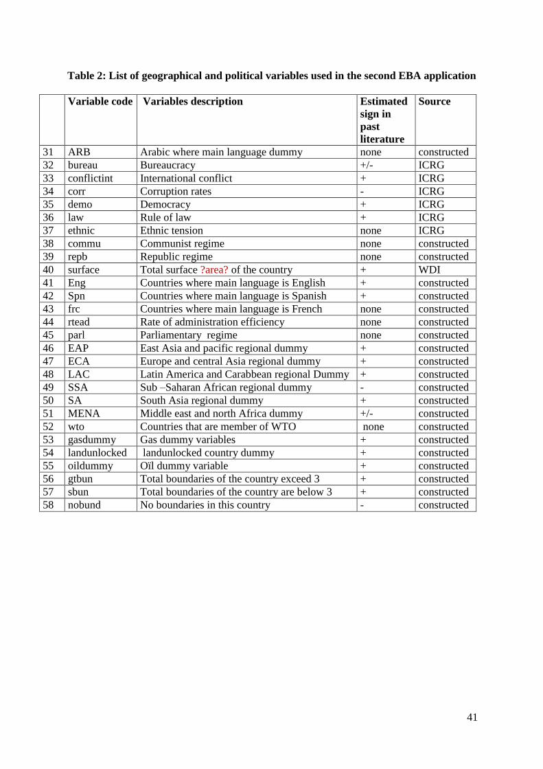
41

Table 2: List of geographical and political variables used in the second EBA application

Variable code Variables description Estimated

sign in

past

literature

Source

31 ARB Arabic where main language dummy none constructed

32 bureau Bureaucracy +/- ICRG

33 conflictint International conflict + ICRG

34 corr Corruption rates - ICRG

35 demo Democracy + ICRG

36 law Rule of law + ICRG

37 ethnic Ethnic tension none ICRG

38 commu Communist regime none constructed

39 repb Republic regime none constructed

40 surface Total surface ?area? of the country + WDI

41 Eng Countries where main language is English + constructed

42 Spn Countries where main language is Spanish + constructed

43 frc Countries where main language is French none constructed

44 rtead Rate of administration efficiency none constructed

45 parl Parliamentary regime none constructed

46 EAP East Asia and pacific regional dummy + constructed

47 ECA Europe and central Asia regional dummy + constructed

48 LAC Latin America and Carabbean regional Dummy + constructed

49 SSA Sub –Saharan African regional dummy - constructed

50 SA South Asia regional dummy + constructed

51 MENA Middle east and north Africa dummy +/- constructed

52 wto Countries that are member of WTO none constructed

53 gasdummy Gas dummy variables + constructed

54 landunlocked landunlocked country dummy + constructed

55 oildummy Oïl dummy variable + constructed

56 gtbun Total boundaries of the country exceed 3 + constructed

57 sbun Total boundaries of the country are below 3 + constructed

58 nobund No boundaries in this country - constructed

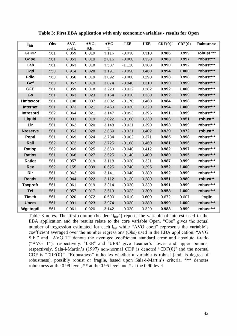
42

Table 3: First EBA application with only economic variables - results for Open

Obs AVG

coeft.

AVG

S.E.

AVG

T

( ) ( ) Robustness

GDPP 561 0.059 0.019 3.116 -0.030 0.310 0.986 0.999 robust ***

Gdpg 561 0.053 0.019 2.816 -0.060 0.330 0.983 0.997 robust***

Cab 561 0.063 0.018 3.587 -1.110 0.380 0.990 0.992 robust***

Cgd 558 0.914 0.028 3.191 -0.090 0.460 0.994 1.000 robust***

Fdio 560 0.056 0.019 3.092 -0.080 0.290 0.993 0.998 robust***

Gcf 560 0.057 0.019 3.074 -0.040 0.310 0.990 0.999 robust***

GFE 561 0.059 0.018 3.223 -0.032 0.282 0.992 1.000 robust***

Gs 561 0.063 0.023 3.154 -0.010 0.330 0.992 0.999 robust***

Hmtaxcor 561 0.108 0.037 3.002 -0.170 0.460 0.984 0.998 robust***

Internet 561 0.073 0.021 3.450 -0.030 0.320 0.994 1.000 robust***

Intresprd 562 0.064 0.021 3.147 -0.093 0.396 0.991 0.999 robust***

Liquid 561 0.031 0.019 2.022 -0.168 0.330 0.906 0.951 robust**

Lir 561 0.062 0.020 3.148 -0.031 0.390 0.993 0.999 robust***

Nreserve 561 0.053 0.028 2.659 -0.331 0.402 0.929 0.972 robust**

Poptl 561 0.069 0.024 2.734 -0.062 0.371 0.985 0.998 robust***

Rail 562 0.072 0.027 2.725 -0.168 0.460 0.981 0.996 robust***

Ratiop 562 0.069 0.025 2.660 -0.040 0.412 0.982 0.997 robust***

Ratios 561 0.068 0.027 2.525 -0.140 0.400 0.980 0.995 robust***

Ratiot 561 0.057 0.019 3.118 -0.030 0.321 0.987 0.999 robust***

Rex 562 0.155 0.039 0.625 -0.740 0.295 0.952 1.000 robust***

Rir 561 0.062 0.020 3.141 -0.040 0.380 0.992 0.999 robust***

Roads 561 0.044 0.022 2.112 -0.120 0.280 0.951 0.980 robust**

Taxprofr 561 0.061 0.019 3.314 -0.030 0.330 0.991 0.999 robust***

Tel 561 0.057 0.017 2.519 -0.023 0.300 0.958 1.000 robust***

Timeb 561 0.020 0.072 0.500 -0.610 0.600 0.672 0.607 fragile

Unem 561 0.091 0.023 3.974 -0.020 0.380 0.999 1.000 robust***

Wgetogdl 561 0.061 0.020 3.142 -0.030 0.320 0.988 0.999 robust***

Table 3 notes. The first column (headed ) reports the variable of interest used in the

EBA application and the results relate to the core variable Open. “Obs” gives the actual

number of regression estimated for each while “AVG coeft” represents the variable’s

coefficient averaged over the number regressions (Obs) used in the EBA application. “AVG

S.E.” and “AVG T” denote the averaged coefficient standard error and absolute t-ratio

(“AVG T”), respectively. and give Leamer’s lower and upper bounds,

respectively. Sala-i-Martin’s (1997) non-normal CDF is denoted “ ( ) and the normal

CDF is “ ( )”. “Robustness” indicates whether a variable is robust (and its degree of

robustness), possibly robust or fragile, based upon Sala-i-Martin’s criteria. *** denotes

robustness at the 0.99 level, ** at the 0.95 level and * at the 0.90 level.

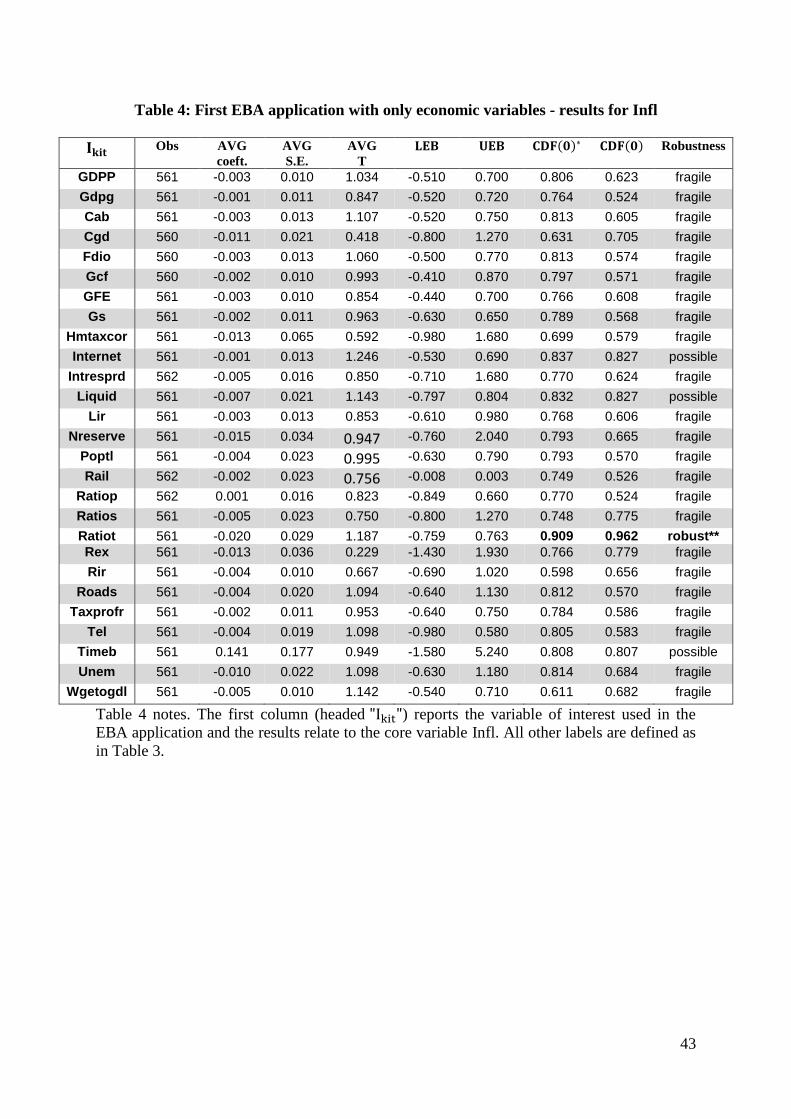
43

Table 4: First EBA application with only economic variables - results for Infl

Obs AVG

coeft.

AVG

S.E.

AVG

T

( ) ( ) Robustness

GDPP 561 -0.003 0.010 1.034 -0.510 0.700 0.806 0.623 fragile

Gdpg 561 -0.001 0.011 0.847 -0.520 0.720 0.764 0.524 fragile

Cab 561 -0.003 0.013 1.107 -0.520 0.750 0.813 0.605 fragile

Cgd 560 -0.011 0.021 0.418 -0.800 1.270 0.631 0.705 fragile

Fdio 560 -0.003 0.013 1.060 -0.500 0.770 0.813 0.574 fragile

Gcf 560 -0.002 0.010 0.993 -0.410 0.870 0.797 0.571 fragile

GFE 561 -0.003 0.010 0.854 -0.440 0.700 0.766 0.608 fragile

Gs 561 -0.002 0.011 0.963 -0.630 0.650 0.789 0.568 fragile

Hmtaxcor 561 -0.013 0.065 0.592 -0.980 1.680 0.699 0.579 fragile

Internet 561 -0.001 0.013 1.246 -0.530 0.690 0.837 0.827 possible

Intresprd 562 -0.005 0.016 0.850 -0.710 1.680 0.770 0.624 fragile

Liquid 561 -0.007 0.021 1.143 -0.797 0.804 0.832 0.827 possible

Lir 561 -0.003 0.013 0.853 -0.610 0.980 0.768 0.606 fragile

Nreserve 561 -0.015 0.034 0.947 -0.760 2.040 0.793 0.665 fragile

Poptl 561 -0.004 0.023 0.995 -0.630 0.790 0.793 0.570 fragile

Rail 562 -0.002 0.023 0.756 -0.008 0.003 0.749 0.526 fragile

Ratiop 562 0.001 0.016 0.823 -0.849 0.660 0.770 0.524 fragile

Ratios 561 -0.005 0.023 0.750 -0.800 1.270 0.748 0.775 fragile

Ratiot 561 -0.020 0.029 1.187 -0.759 0.763 0.909 0.962 robust**

Rex 561 -0.013 0.036 0.229 -1.430 1.930 0.766 0.779 fragile

Rir 561 -0.004 0.010 0.667 -0.690 1.020 0.598 0.656 fragile

Roads 561 -0.004 0.020 1.094 -0.640 1.130 0.812 0.570 fragile

Taxprofr 561 -0.002 0.011 0.953 -0.640 0.750 0.784 0.586 fragile

Tel 561 -0.004 0.019 1.098 -0.980 0.580 0.805 0.583 fragile

Timeb 561 0.141 0.177 0.949 -1.580 5.240 0.808 0.807 possible

Unem 561 -0.010 0.022 1.098 -0.630 1.180 0.814 0.684 fragile

Wgetogdl 561 -0.005 0.010 1.142 -0.540 0.710 0.611 0.682 fragile

Table 4 notes. The first column (headed ) reports the variable of interest used in the

EBA application and the results relate to the core variable Infl. All other labels are defined as

in Table 3.

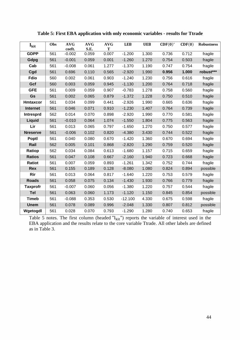
44

Table 5: First EBA application with only economic variables - results for Ttrade

Obs AVG

coeft.

AVG

S.E.

AVG

T

( ) ( ) Robustness

GDPP 561 -0.002 0.059 0.007 -1.200 1.300 0.736 0.712 fragile

Gdpg 561 -0.001 0.059 0.001 -1.260 1.270 0.754 0.503 fragile

Cab 561 -0.008 0.061 1.277 -1.370 1.190 0.747 0.754 fragile

Cgd 561 0.696 0.110 0.565 -2.920 1.990 0.956 1.000 robust***

Fdio 560 0.002 0.061 0.903 -1.240 1.230 0.756 0.616 fragile

Gcf 560 0.003 0.059 0.945 -1.130 1.200 0.764 0.718 fragile

GFE 561 0.009 0.059 0.907 -0.783 1.278 0.758 0.560 fragile

Gs 561 0.002 0.065 0.879 -1.372 1.228 0.750 0.510 fragile

Hmtaxcor 561 0.034 0.099 0.441 -2.926 1.990 0.665 0.636 fragile

Internet 561 0.046 0.071 0.910 -1.230 1.407 0.764 0.739 fragile

Intresprd 562 0.014 0.070 0.898 -2.920 1.990 0.770 0.581 fragile

Liquid 561 -0.010 0.064 1.074 -1.550 1.804 0.775 0.563 fragile

Lir 561 0.013 0.065 0.797 -1.650 1.270 0.750 0.577 fragile

Nreserve 561 -0.006 0.102 0.820 -4.380 3.430 0.744 0.522 fragile

Poptl 561 0.040 0.080 0.670 -1.420 1.360 0.670 0.694 fragile

Rail 562 0.005 0.101 0.868 -2.820 1.290 0.759 0.520 fragile

Ratiop 562 0.034 0.084 0.613 -1.680 1.157 0.715 0.659 fragile

Ratios 561 0.047 0.108 0.667 -2.160 1.940 0.723 0.668 fragile

Ratiot 561 0.007 0.059 0.893 -1.261 1.342 0.752 0.744 fragile

Rex 561 0.155 0.189 0.128 -8.080 1.080 0.824 0.894 possible

Rir 561 0.013 0.064 0.817 -1.640 1.220 0.753 0.579 fragile

Roads 561 0.058 0.075 0.134 -1.430 1.930 0.766 0.779 fragile

Taxprofr 561 -0.007 0.060 0.056 -1.380 1.220 0.757 0.544 fragile

Tel 561 0.063 0.060 1.173 -1.120 1.150 0.845 0.854 possible

Timeb 561 -0.088 0.353 0.530 -12.100 4.330 0.675 0.598 fragile

Unem 561 0.078 0.089 0.996 -2.048 1.330 0.807 0.812 possible

Wgetogdl 561 0.028 0.070 0.793 -1.290 1.280 0.740 0.653 fragile

Table 5 notes. The first column (headed ) reports the variable of interest used in the

EBA application and the results relate to the core variable Ttrade. All other labels are defined

as in Table 3.

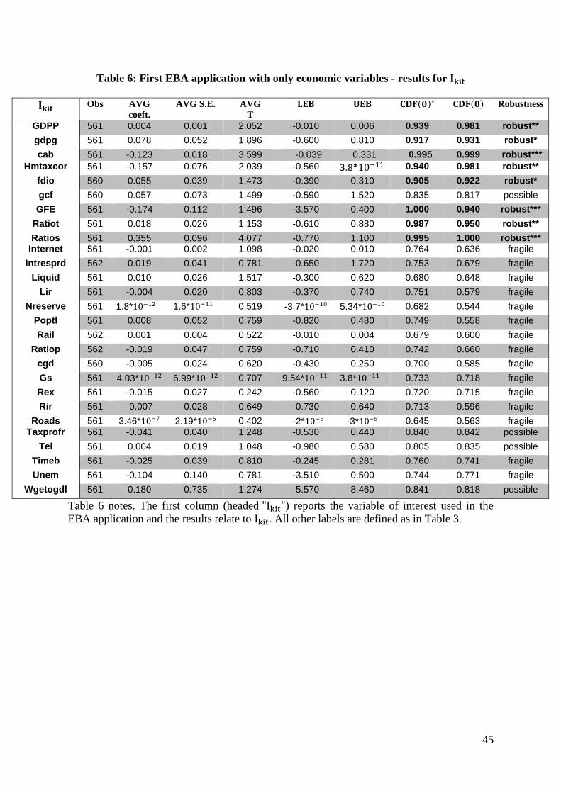
45

Table 6: First EBA application with only economic variables - results for

Obs AVG

coeft.

AVG S.E. AVG

T

( ) ( ) Robustness

GDPP 561 0.004 0.001 2.052 -0.010 0.006 0.939 0.981 robust**

gdpg 561 0.078 0.052 1.896 -0.600 0.810 0.917 0.931 robust*

cab 561 -0.123 0.018 3.599 -0.039 0.331 0.995 0.999 robust***

Hmtaxcor 561 -0.157 0.076 2.039 -0.560 3.8* 0.940 0.981 robust**

fdio 560 0.055 0.039 1.473 -0.390 0.310 0.905 0.922 robust*

gcf 560 0.057 0.073 1.499 -0.590 1.520 0.835 0.817 possible

GFE 561 -0.174 0.112 1.496 -3.570 0.400 1.000 0.940 robust***

Ratiot 561 0.018 0.026 1.153 -0.610 0.880 0.987 0.950 robust**

Ratios 561 0.355 0.096 4.077 -0.770 1.100 0.995 1.000 robust*** Internet 561 -0.001 0.002 1.098 -0.020 0.010 0.764 0.636 fragile

Intresprd 562 0.019 0.041 0.781 -0.650 1.720 0.753 0.679 fragile

Liquid 561 0.010 0.026 1.517 -0.300 0.620 0.680 0.648 fragile

Lir 561 -0.004 0.020 0.803 -0.370 0.740 0.751 0.579 fragile

Nreserve 561 1.8* 1.6* 0.519 -3.7* 5.34* 0.682 0.544 fragile

Poptl 561 0.008 0.052 0.759 -0.820 0.480 0.749 0.558 fragile

Rail 562 0.001 0.004 0.522 -0.010 0.004 0.679 0.600 fragile

Ratiop 562 -0.019 0.047 0.759 -0.710 0.410 0.742 0.660 fragile

cgd 560 -0.005 0.024 0.620 -0.430 0.250 0.700 0.585 fragile

Gs 561 4.03* 6.99* 0.707 9.54* 3.8* 0.733 0.718 fragile

Rex 561 -0.015 0.027 0.242 -0.560 0.120 0.720 0.715 fragile

Rir 561 -0.007 0.028 0.649 -0.730 0.640 0.713 0.596 fragile

Roads 561 3.46* 2.19* 0.402 -2* -3* 0.645 0.563 fragile

Taxprofr 561 -0.041 0.040 1.248 -0.530 0.440 0.840 0.842 possible

Tel 561 0.004 0.019 1.048 -0.980 0.580 0.805 0.835 possible

Timeb 561 -0.025 0.039 0.810 -0.245 0.281 0.760 0.741 fragile

Unem 561 -0.104 0.140 0.781 -3.510 0.500 0.744 0.771 fragile

Wgetogdl 561 0.180 0.735 1.274 -5.570 8.460 0.841 0.818 possible

Table 6 notes. The first column (headed ) reports the variable of interest used in the

EBA application and the results relate to . All other labels are defined as in Table 3.

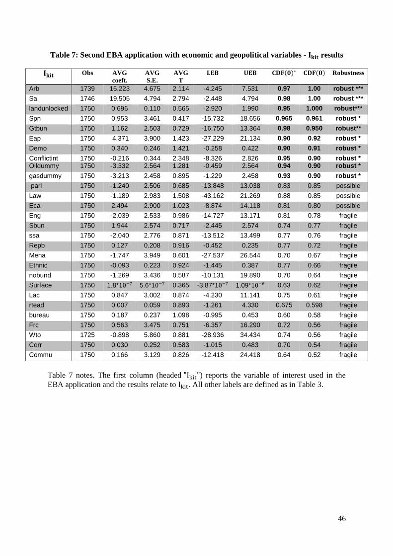
46

Table 7: Second EBA application with economic and geopolitical variables - results

Obs AVG

coeft.

AVG

S.E.

AVG

T

( ) ( ) Robustness

Arb 1739 16.223 4.675 2.114 -4.245 7.531 0.97 1.00 robust ***

Sa 1746 19.505 4.794 2.794 -2.448 4.794 0.98 1.00 robust ***

landunlocked 1750 0.696 0.110 0.565 -2.920 1.990 0.95 1.000 robust***

Spn 1750 0.953 3.461 0.417 -15.732 18.656 0.965 0.961 robust *

Gtbun 1750 1.162 2.503 0.729 -16.750 13.364 0.98 0.950 robust**

Eap 1750 4.371 3.900 1.423 -27.229 21.134 0.90 0.92 robust *

Demo 1750 0.340 0.246 1.421 -0.258 0.422 0.90 0.91 robust *

Conflictint 1750 -0.216 0.344 2.348 -8.326 2.826 0.95 0.90 robust * Oildummy 1750 -3.332 2.564 1.281 -0.459 2.564 0.94 0.90 robust *

gasdummy 1750 -3.213 2.458 0.895 -1.229 2.458 0.93 0.90 robust *

parl 1750 -1.240 2.506 0.685 -13.848 13.038 0.83 0.85 possible

Law 1750 -1.189 2.983 1.508 -43.162 21.269 0.88 0.85 possible

Eca 1750 2.494 2.900 1.023 -8.874 14.118 0.81 0.80 possible

Eng 1750 -2.039 2.533 0.986 -14.727 13.171 0.81 0.78 fragile

Sbun 1750 1.944 2.574 0.717 -2.445 2.574 0.74 0.77 fragile

ssa 1750 -2.040 2.776 0.871 -13.512 13.499 0.77 0.76 fragile

Repb 1750 0.127 0.208 0.916 -0.452 0.235 0.77 0.72 fragile

Mena 1750 -1.747 3.949 0.601 -27.537 26.544 0.70 0.67 fragile

Ethnic 1750 -0.093 0.223 0.924 -1.445 0.387 0.77 0.66 fragile

nobund 1750 -1.269 3.436 0.587 -10.131 19.890 0.70 0.64 fragile

Surface 1750 1.8* 5.6* 0.365 -3.87* 1.09* 0.63 0.62 fragile

Lac 1750 0.847 3.002 0.874 -4.230 11.141 0.75 0.61 fragile

rtead 1750 0.007 0.059 0.893 -1.261 4.330 0.675 0.598 fragile

bureau 1750 0.187 0.237 1.098 -0.995 0.453 0.60 0.58 fragile

Frc 1750 0.563 3.475 0.751 -6.357 16.290 0.72 0.56 fragile

Wto 1725 -0.898 5.860 0.881 -28.936 34.434 0.74 0.56 fragile

Corr 1750 0.030 0.252 0.583 -1.015 0.483 0.70 0.54 fragile

Commu 1750 0.166 3.129 0.826 -12.418 24.418 0.64 0.52 fragile

Table 7 notes. The first column (headed ) reports the variable of interest used in the

EBA application and the results relate to . All other labels are defined as in Table 3.

47

Table 8: Second EBA application with economic and geopolitical variables - results

Obs AVG coeft.

AVG S.E. AVG T

( ) ( ) Robustness

Fdio 1313 0.733 0.050 50.477 -0.740 0.233 0.985 1.000 robust***

Cgd 1311 0.7330 0.0505 50.477 -0.740 0.233 0.985 1.000 robust***

Cab 1313 -0.123 0.018 3.599 -0.039 0.331 0.995 0.999 robust***

Internet 1311 0.010 0.004 1.327 -0.044 0.020 0.984 0.988 robust**

Gdpp 1313 0.004 0.001 2.052 -0.010 0.006 0.939 0.981 robust**

Ratiot 1520 -5.718 3.441 1.516 -51.899 21.403 0.907 0.950 robust**

Tel 1521 0.010 0.006 1.534 -0.010 0.006 0.919 0.944 robust**

Gdpg 1313 0.078 0.052 1.896 -0.600 0.810 0.917 0.931 robust*

Liquid 1311 0.011 0.009 1.323 -0.050 0.012 0.841 0.892 possible

Gcf 1311 0.161 0.143 2.826 -1.192 1.808 0.870 0.869 possible

Taxprofr 1088 -0.041 0.040 1.248 -0.530 0.440 0.840 0.842 possible

Poptl 1311 0.196 0.232 1.166 -2.025 1.304 0.814 0.800 possible

Hmtaxcor 1520 -0.202 0.216 0.849 -3.510 0.500 0.744 0.771 fragile

Rir 1636 0.017 0.030 0.600 -0.087 0.030 0.583 0.716 fragile

Rex 1311 -0.020 0.058 0.665 -0.914 0.871 0.722 0.715 fragile

Unem 1088 0.069 0.139 0.831 -0.327 1.900 0.753 0.691 fragile

Ttrade 1331 -0.021 0.043 0.801 -0.242 0.109 0.753 0.684 fragile

Intresprd 1311 0.019 0.041 0.781 -0.650 1.720 0.753 0.679 fragile

Roads 1331 8.509* 2.212* 0.398 -6.247* 4.673* 0.647 0.649 fragile

Nreserve 1520 5.989* 1.858* 0.610 -4.628* 3.527* 0.708 0.626 fragile

Wgetogdl 1520 -8.698 37.807 0.707 -85.473 103.13 0.726 0.591 fragile

Lir 1311 0.004 0.027 0.593 -0.148 0.096 0.696 0.579 fragile

Rail 1311 7.076* 3.767* 0.426 -0.0003 0.0002 0.655 0.574 fragile

Gs 1311 -4.309* 2.509* 0.475 -6.057* 4.546* 0.670 0.568 fragile

Timeb 1141 -0.002 0.013 0.898 -0.028 0.017 0.787 0.562 fragile

Inflation 1311 -0.005 0.036 0.477 -1.335 1.374 0.668 0.560 fragile

Ratiop 1520 3.939* 0.003 0.300 -0.007 0.009 0.610 0.504 fragile

Table 8 notes. The first column (headed ) reports the variable of interest used in the

EBA application and the results relate to . All other labels are defined as in Table 3.